W&M ScholarWorks W&M ScholarWorks

Undergraduate Honors Theses Theses, Dissertations, & Master Projects

5-2019

The Effects of Tax Revenue Changes on Economic Growth The Effects of Tax Revenue Changes on Economic Growth

Xiangwen Sun

Follow this and additional works at: https://scholarworks.wm.edu/honorstheses

Part of the Economics Commons

Recommended Citation Recommended Citation Sun, Xiangwen, "The Effects of Tax Revenue Changes on Economic Growth" (2019). Undergraduate Honors Theses. Paper 1424. https://scholarworks.wm.edu/honorstheses/1424

This Honors Thesis is brought to you for free and open access by the Theses, Dissertations, & Master Projects at W&M ScholarWorks. It has been accepted for inclusion in Undergraduate Honors Theses by an authorized administrator of W&M ScholarWorks. For more information, please contact scholarworks@wm.edu.

Page ! of !1 25

The Effect of Tax Policy on Economic Growth

Introduction

On December 22, 2017, President Trump signed the Tax Cut and Job Act of 2017(TCJA).

This act cut the corporate income tax from 35% to 21%, and lowered most individual income tax

rates, including the top marginal rate from 39.6% to 37%. Trump stated that the decrease of tax

rate would draw more investment back to the U.S. and increase the tax base. It will ensure the

government tax revenue while boosting the U.S. economy. However, the joint committee of

taxation predicted that the tax cut would only increase U.S. annual growth rate by roughly 0.08

percent. This research focus on developing model to examine the effect of tax revenue on

economic growth.

This research includes two analysis on the how tax policy affects economic growth. First,

the first method employs a time-series linear regression on real GDP and uses policy dummy

variables to detect the effects of those policy. Then it also uses Bai-Perron test to examine

whether there is a structural break for each time there is a tax policy change. Second, I used the

Structural Vector Autoregression Model to estimate the effects of personal and corporate income

tax on real GDP. The model included the 5 benchmark variables (GDP, interest rate, price level,

government spending, tax revenue). Through the impulse function, the research would gave

analysis on how two targeted variable affects economic growth.

The first section of this research shows that, among the five major tax policy tested,

Reagan Tax Cut of 1981, Tax Reduction Act of 1975(temporary) and Trump’s recent Tax Cut and

Job Act are significant in predicting the real GDP changes. All of these three policies shows a

Page ! of !2 25

positive influence on real GDP. Furthermore, there are structural breaks presented in real GDP

data, but none of them corresponds to tax policy changes. The result indicates that tax policy

does not perform a structural changes in how the independent variables in the time-series

analysis impacting the real GDP.

Results from the second section does not produce significant results for the effects of

corporate income tax and personal income on economic growth. Corporate income tax shock has

a short term negative influence on real GDP, but becomes not significantly different from zero

after the third quarter. Personal Income tax revenue does not show a significant effects on the

economy.

Literature Review

Model

Structural Break

In order to determine whether a policy had significant structural influence on the current

trend of GDP, we need to detect whether there is a structural break before and after the enactment

of this policy. In other terms, whether there is a significant change in the coefficient or a portion

of the coefficient of the independent variable before and after specific dates.

Chow developed a method to detect whether a known exogenous break date would give a

structural break based on F-statistics(Chow 1960). Quandt then used the chow test to iterate on

all possible break points and enabled detection of structural break even without a known

breakpoint by finding the maximum Chow statistics (Quandt 1960). Quandt’s method was

computationally burdensome and not widely used as the limiting distribution of the test

Page ! of !3 25

statistic was unknown, until Andrews and Ploberg later advanced the method with an applicable

distribution for the test-statistic (Andrews & Ploberg 1994). However, a critique for the previous

tests is that they ignore other possible breakpoints that are within data timeframe. Two methods

were invented to solve this problem and to detect multiple structural breaks: the joint testing

method and the sequential method. The joint testing method would iterate all possible breakpoint

options based on the number of breaks, thus when testing for more than 2 breaks, the run time for

joint method would be so large and infeasible. However, Bai and Perron’s sequential method,

based on dynamic programming, is able to detect multiple structural break with unknown break

dates, as they separate the sample into subsamples each time the algorithm finds a

breakpoint(Bai & Perron 1998, 2003).

Before Bai & Perron’s method, researchers could test for multiple structural breaks by

trimming the data into different subsamples and then perform the chow test for structural breaks.

However, the breakpoints might have potential endogeneity problem. Bai-Perron test

successfully solved this problem as it finds the breakpoints sequentially between the selected test

dates. Bai-Perron test also has a much efficient run time than other methods, thus this research

uses Bai-Perron test for multiple structural breaks.

Structural Vector Autoregression Model

In previous literatures, there are typically four different approaches researchers used VAR

model for analyzing fiscal policies, a narrative approach, a sign-restriction on impulse function

approach, a mathematical approach (Choleski), and an exploiting decision lags approach. As

explored by Perotti(2002), each approach has its distinct advantages and limitation.

Page ! of !4 25

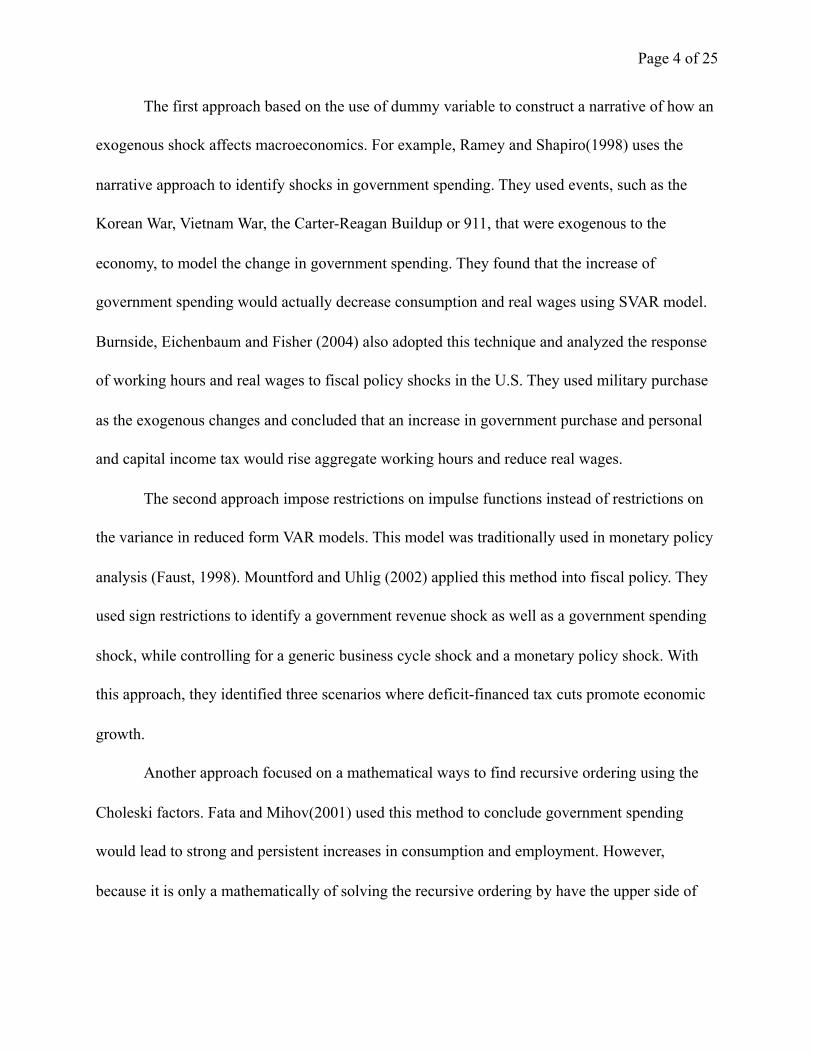
The first approach based on the use of dummy variable to construct a narrative of how an

exogenous shock affects macroeconomics. For example, Ramey and Shapiro(1998) uses the

narrative approach to identify shocks in government spending. They used events, such as the

Korean War, Vietnam War, the Carter-Reagan Buildup or 911, that were exogenous to the

economy, to model the change in government spending. They found that the increase of

government spending would actually decrease consumption and real wages using SVAR model.

Burnside, Eichenbaum and Fisher (2004) also adopted this technique and analyzed the response

of working hours and real wages to fiscal policy shocks in the U.S. They used military purchase

as the exogenous changes and concluded that an increase in government purchase and personal

and capital income tax would rise aggregate working hours and reduce real wages.

The second approach impose restrictions on impulse functions instead of restrictions on

the variance in reduced form VAR models. This model was traditionally used in monetary policy

analysis (Faust, 1998). Mountford and Uhlig (2002) applied this method into fiscal policy. They

used sign restrictions to identify a government revenue shock as well as a government spending

shock, while controlling for a generic business cycle shock and a monetary policy shock. With

this approach, they identified three scenarios where deficit-financed tax cuts promote economic

growth.

Another approach focused on a mathematical ways to find recursive ordering using the

Choleski factors. Fata and Mihov(2001) used this method to conclude government spending

would lead to strong and persistent increases in consumption and employment. However,

because it is only a mathematically of solving the recursive ordering by have the upper side of

Page ! of !5 25

the matrix to be zero. It would add implicit restrictions when applying to actual economics

models.

The last approach is the structural VAR model pioneered by Blanchard and Perotti(2002).

They focused on exploiting decision lags in fiscal policy and institutional information about the

elasticity of variables to economic activities. Blanchard and Perotti(2002) expanded on this

method further and found the effects of fiscal policy on economic growth has became smaller in

the past years. Arin (2005) also expanded on the same model to explore effects of defense

spending , government expenditure and tax revenue on economic growth. Auerbach and

Gorodnichenko (2012) also used this method to analyze the size of fiscal multipliers when the

economy is in recession.

Effects of Tax on Economy: Other Models

Previous researches have conflicting results on the effects of tax structure on economic

growth. Yongzheng Liu and Jorge Martinez-Vazquez researched on the growth-inequality

tradeoff based on tax structure and found that income tax led to growth while corporate tax

jeopardized it (2015), which contradicts with Lighter and Zhang’s finding that raising corporate

tax increase GDP the most, whereas increase individual income harms the economy(2015).

Akgun, Cournede, and Fournier showed that reducing corporate tax and personal income tax

while raising recurrent property and consumption tax could boost GDP growth(2017). Their

study echos with Galindo and Pombo’s study and Blochliger’s study that taxes on corporate or

personal income reduce incentives to raise supply; whereas property tax have no disincentive

effects (Galindo 2011, Blochliger 2015).

Page ! of !6 25

Data

This research uses data from 1960 first quarter to 2018 forth quarter. The research

included quarterly data instead of annual data with the assumption that fiscal policy can be

adjusted in response to unexpected changes within the year (Blanchard & Perotti ,2002). The

data started from 1960 to exclude spike changes in tax revenue resulting from a after war

insurance benefit payment from National Service Life to veterans and also the unusual changes

in government expenditure during the Korean War (1951-1952).

The data are obtain through two different sources. From the Federal Reserve Economic

Data (Fred St.Louis), we obtain data for real GDP, nominal GDP, 3-month Treasury Bill, private

investment and CPI index. The GDP deflator is calculated by dividing nominal GDP by real

GDP. The other source is Bureau of Economic Analysis, in which I obtained the data for personal

and corporate income tax revenue, government expenditure. The CPI index, personal and

corporate income tax revenue, investment and government expenditure are all deflated with the

GDP deflator to control for inflation. The first section of this research only uses the real GDP

data collected, and the second section of this research uses all the data presented.

Section 1 — Structural Break

Method

In this section, the research focuses on detecting structural breaks and also test whether

each tax policy has affected the growth of real GDP. Between the timeframe of the data (from

Page ! of !7 25

1960Q1 to 2018Q4), there were 4 major tax policies enacted, including Kennedy Tax Reduction

Act of 1964(Q2), Tax Reduction Act of 1975(Q2)[temporary], Reagan Tax Cut of 1981 (Q4) and

1986 (1987Q1), and Trump’s tax cut in 2017(Q4). If the policy changes have significantly affect

the growth rate afterwards, we would expected to see multiple structural breaks. In order to

control for the potential endogeneity between each breakpoint, I use the Bai-Perron Test to

conduct the research.

First, I constructed a time-series linear regression for real GDP data. Because the model

focus on the finding the change in mean, I regress the real GDP data on a constant, a lag, and

also a trend. I also create dummy variables for four tax policies changes to check their influence

on the trend. Furthermore, I include seasonal dummies to check for seasonality. Because this

model allow for serial correlation in the error terms, we specify a quadratic spectral kernel based

on HAC covariance estimation using prewritten residuals. The kernel bandwidth would be

determined automatically by the Andrews AR(1) method. I select the maximum number of 5

breaks for the data as it is the maximum selection option in Eviews. Then, I conduct the multiple

breakpoint tests based on the global information criteria, and also the sequential determined

method.

The global optimization procedures aims for identifying the number of multiple breaks

and their associated coefficient to minimize the sums-of-squared residuals of the regression

model. The detailed procedures for the method are as following. With a pre-specify a maximum

number of breakpoint, it first test for the optimal number of breakpoints by finding the number of

breakpoints, m, that minimize the specified information criteria. Then, it finds the m breakpoints

sequentially. It begin with the full sample and then perform a test of parameter constancy with

Page ! of !8 25

unknown break. After finding the first break, it then test for structural breakpoints in breakpoint

tests in each subsamples and add breakpoint when the null for non break is rejected. The test then

repeat the procedure until it finds m breakpoints. The sequential method started like the

sequential process in global information method, and then perform a reduction.

Result & Discussion

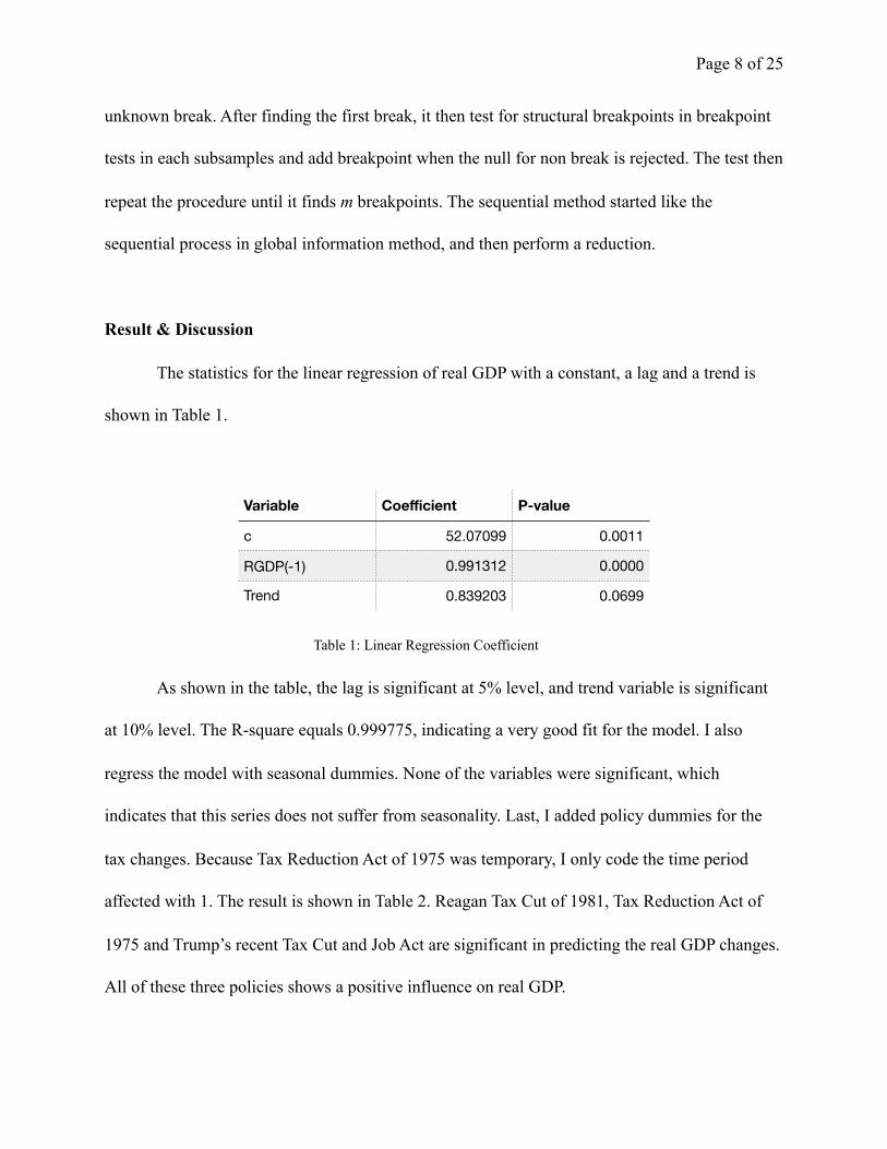
The statistics for the linear regression of real GDP with a constant, a lag and a trend is

shown in Table 1.

Table 1: Linear Regression Coefficient

As shown in the table, the lag is significant at 5% level, and trend variable is significant

at 10% level. The R-square equals 0.999775, indicating a very good fit for the model. I also

regress the model with seasonal dummies. None of the variables were significant, which

indicates that this series does not suffer from seasonality. Last, I added policy dummies for the

tax changes. Because Tax Reduction Act of 1975 was temporary, I only code the time period

affected with 1. The result is shown in Table 2. Reagan Tax Cut of 1981, Tax Reduction Act of

1975 and Trump’s recent Tax Cut and Job Act are significant in predicting the real GDP changes.

All of these three policies shows a positive influence on real GDP.

Variable Coefficient P-value

c 52.07099 0.0011

RGDP(-1) 0.991312 0.0000

Trend 0.839203 0.0699

Page ! of !9 25

Table 2: Tax Policies’ Effect on Economic Growth

The results for the multiple breakpoints test for real GDP are shown in Table 3. Both the

Schwarz criterion and LWZ criterion indicates that there would be 2 breakpoints. The estimated

breakpoints are 1996Q2 and 2008Q4.

Table 3: Results of Multiple Breakpoint Tests

According to Table 3, none of tax policy changes date seems to correspond to the

structural breakpoints identified by multiple break point tests. It means that none of the tax

policy changes how the independent variables affect real GDP. Two of the policy dummies are

significant indicating that the policy itself might have a positive effect on real GDP after enacted.

Variable Coefficient P-Value

Kennedy Tax Reduction Act (1964) 2.967557 0.8495

Tax Reduction Act (1975)[temporary] 33.20466 0.0157

Reagan Tax Cut of 1981 57.56635 0.0287

Reagan Tax Cut of 1986 -5.689579 0.7946

Trump’s TCJA in 2017 33.20466 0.0137

Name # of Breaks Break dates

Global Information Criteria - BIC 2 1996Q2, 2008Q4

Global Information Criteria - LWZ 2 1996Q2, 2008Q4

Sequential Method 2 1996Q2, 2008Q4

Page ! of !10 25

A potential problem of this test is that Breusch-Godfrey test indicates the model suffers

from serial correlation. The serial correlation problem might potentially result in higher number

of structural breaks estimated by the LWZ and Schwarz criterion in the Global Information

Criterion method.

The next section of this research focuses on detecting how changes of corporate income

tax revenue and personal income tax revenue affect economic growth. As shown in this section,

the real GDP variable does have structural breaks over the desired timeframe. Other variables,

such as corporate income tax revenue and personal income tax revenue, that are used in Section

Two always appears to have structural breaks after the Bai-Perron test.

Thus, the research would uses Structural Vector Autoregressive Model to find the

corresponding relationship. The unit root analysis for each variables and their adjustment for the

SVAR model will also be presented in the next section.

Section 2 — Structural Vector Autoregression Model

Method

Independent Variable Measuring Tax

The aim for this research is to analyze the effects of tax changes on economic growth.

The three current types of data that researchers use to measure tax are stationary tax rate,

nominal tax revenue and real tax revenue(adjusted for inflation). Although stationary tax rate and

nominal tax revenue are easy to acquire and use, it does not fully captures economic conditions

of each year. It also would miss many other factors that would affects the research outcome.

Thus, this research choose to use real tax revenue as one of our independent variable.

Page ! of !11 25

Why Structural Vector Autoregression Model

The challenges for real tax revenue, however, is that it would be affected by the economic

condition of the year, and thus would cause problem of simultaneity with other variables such as

real GDP. Thus, we choose to use the Vector Autoregression (VAR) include to the endogenous

effects of our targeted variables to each other. As proven in the first section that there is structural

break in our real GDP variable and also a few other variables. Thus, I choose to implement the

Structural VAR model and use the impulse-response function to analyze how economy reacts to

different tax policies.

Furthermore, Structural VAR model is very suitable for conducting fiscal policy analysis.

First, output stabilization is rarely a predominant reason explaining changes in fiscal policy;

therefore, we can assume there are exogenous fiscal shocks. Second, decision and

implementation lags in fiscal policy imply that there is little response of fiscal policy to

unexpected movement in economic activity. Thus, one can construct estimates of effects of

unexpected movements in activity on fiscal variables and obtain the estimates of fiscal policy

shocks (Blanchard & Quah, 2002).

Procedure

1. Specify the Model Variable

This research uses the commonly used 5 benchmark criteria based on the Keynesian

model to capture the changes in economic growth (GDP). Thus, it includes variables on GDP,

Page ! of !12 25

interest rate, price level, tax revenue, and government expenditure. The interest rate is included

to account for monetary shocks.

2. Test For Stationarity

First, I performed Augmented Dickey Fuller test for all the five variables. Then, we found

that all the variables are non-stationary at its original state. All five variables, however, are

stationary at first difference, with real GDP being stationary of first difference with trend. As a

result, this research would use the difference of each variable in the model. Furthermore, because

all variables are integrated for order one, the pre-condition for conducting a VAR model is

satisfied. The five variables are also traditionally assumed to be affecting each other, the

condition that all variables are endogenous is also fulfilled.

3. Use Schwarz Information Criterion (BIC) To Determine Lag Length

I constructed an unrestricted VAR and found that based on the BIC statistics, including

lag till order one is optimal. The intuition of this test is to find a balance between parsimony with

the reduction sum of square. Thus, avoiding curse of dimensionality.

4. Estimate Reduced Form VAR Model

I then estimate the basic VAR model using lag 1 on each variable, and then use Wald Test

to test for joint significance of the variables, such as whether the two lags for GDP is jointly

significant for personal income tax revenue.

Page ! of !13 25

5. Perform Diagnosis tests

I performed the test for autocorrelation LM test to see whether it suffers from serial

correlation. It shows that except for lag length 1, the data does not suffer from serial correlation.

I also checked the stability of the model. As shown in the graph, all the roots lied inside

the circle, which means the estimated VAR model is stationary. Otherwise, the impulse response

standard error would not be valid.

VAR Residual Serial Correlation Test

Lag Probability

1 0.0122

2 0.4247

3 0.7925

4 0.8139

Page ! of !14 25

6. Structural Identification / Add Restriction

For the structural identification, I imposed the long run restriction as suggested in

Blanchard & Quah(2002) and (Arin & Koray 2005). Structural identification interprets

historically observed variation in data in a way that allows the variation to be used to predict.

7. Use Impulse Function to Model the Effects

Next, I performed the variance decomposition, and then used the impulse functions to

capture the effects of shocks to each variables.

Result & Discussion

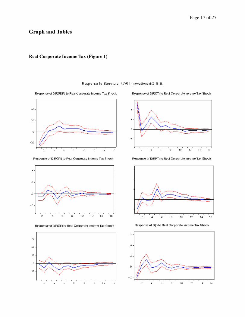
The IRFs of all model variables to a one-standard deviation shock to real personal income

tax, corporate income tax, and real government expenditure are included in Figures 1-3. The

solid blue lines indicate the point estimates, and the red lines shows the one standard deviation

bands.

Figure 1 presents the IRFs of interest rate, real GDP, real corporate income tax, real

persona income tax, price level and real government expenditure to a positive innovation in

corporate income tax. The response of GDP is negative before quarter 2 and positive afterwards.

However, it is not significantly different from zero after quarter 2, which means it only have a

negative influence on GDP in the short term. The response of Corporate income tax is positive

and significantly different from zero for some of the first few quarters, but not significantly

different from zero for the other parts, which means the innovation is not permanent. The

Page ! of !15 25

response of price level and government is not significantly different from zero. The response of

personal income tax is negative and significant at the first quarter and positive and significant in

quarter 5-6, and 7-9, which means corporate income tax would have a negative influence on

personal income tax revenue at first, and then it would have a positive influence then no

influence. The response of interest rate indicates that increase of corporate income tax would

have a negative influence on interest rate only in the short term.

Figure 2 presents the IRFs of interest rate, real GDP, real corporate income tax, real

persona income tax, price level and real government expenditure to a positive innovation in

personal income tax. Based on this figure, the response of GDP, price level, and government

expenditure is not significant. The response of real corporate income tax is positive at first and

then become not significant. The response function of interest rate is only significant for a few

quarters , and it is positively influenced by increase of personal income tax. The response of

personal income tax is not significant, thus the innovation is not permanent.

Figure 3 presents the IRFs of interest rate, real GDP, real corporate income tax, real

persona income tax, price level and real government expenditure to a positive innovation in

government expenditure. The response of GDP is positive and significant at first, and then

become insignificant in the longer run. That means that increase of government expenditure

would have positive influence on GDP only in the short term. The response corporate income tax

is also only significant at the first quarter. The response of price level is positive at first and then

become negative. The response of government expenditure is not always significantly different

from zero which means the innovation is not permanent.

Page ! of !16 25

Conclusion

The first section of this research concludes that, among the five major tax policy tested,

Reagan Tax Cut of 1981, Tax Reduction Act of 1975(temporary) and Trump’s recent Tax Cut and

Job Act did have positive influence on economic growth. However, tax policies does not perform

a structural changes for GDP, which means it does not change how other variables affect GDP.

The results from the second section shows that corporate income tax shock only has a short term

negative influence on real GDP, but becomes not significantly different from zero after the third

quarter. Personal Income tax revenue does not show a significant effects on the economy.

Page ! of !17 25

Graph and Tables

Real Corporate Income Tax (Figure 1)

Page ! of !18 25

Real Personal Income Tax (Figure 3)

Page ! of !19 25

Real Government Expenditure (Figure 1) [1-r; 2-gdp, 3-corpT, 4-persT, 5-CPI, 6-GovtExp]

Page ! of !20 25

Residuals

Page ! of !21 25

Page ! of !22 25

Reference

Auerbach, A. “ Capital Gains Taxation in the United States: Realizations, Revenue, and

Rhetoric.” The Brookings Institute, 1988, No.2

_____ , “ Capital Gains Taxation and Tax Reform.” National Tax Journal, Vol. 42, no. 3,

(September, 1989), pp. 391-401

Auerbach, A. & Slemrod, J. “The Economic Effects of the Tax Reform Act of 1986.” Journal of

Economic Literature, 1997, June. Vol. 35, No. 2, pp. 589-632

Akgun, O., B. Cournède and J. Fournier, “The effects of the tax mix on inequality and growth”,

OECD Economics Department Working Papers, 2017, No. 1447, OECD Publishing,

Paris.

Andrews, D.W.K, “Testing for structural instability and structural change with unknown change

point.” Econometrica 61, 1993, 821-856

Andrews, D. W. K. & Ploberger. W “Optimal Tests When a Nuisance Parameter Is Present Only

Under the Alternative.” Econometrica 62, no. 6 1994: 1383-414.

_____ , “Optimal changepoint tests for normal linear regression.” Journal of Econometrics 70,

1996, 9-38

Arin, P. & Koray, F, “Fiscal Policy and Economic Activity: U.S. Evidence,” Macroeconomics

0508024, University Library of Munich, Germany

Bai, J. “Estimating Multiple Breaks One at a Time.” Econometric Theory 13, 1997, 315-252.

Bai, J and Perron, P. “Estimating and Testing Linear Models with Multiple Structural Changes.”

Econometrica 66, 1998, 47-78.

Page ! of !23 25

_____ “Computation and Analysis of Multiple Structural Change Models.” Journal of Applied

Econometrics 18, 2003, 1-22.

Blanchard, O. “Fiscal Policy in General Equilibrium,” American Economic Review, 1989, 79(5),

1146-1164

Blanchard, O. and Perotti, R. "An Empirical Characterization of the Dynamic Effects of Changes

in Government Spending and Taxes on Output." The Quarterly Journal of

Economics 117, no. 4, 2002: 1329-368.

Blöchliger, H. “Reforming the Tax on Immovable Property: Taking Care of the Unloved”, OECD

Economics Department Working Papers, 2015: No. 1205, OECD Publishing, Paris.

Burnside, Craig & Eichenbaum, Martin & Fisher, Jonas D. M., “Fiscal Shocks and their

consequences,” Journal of Economic Theory, Elsevier, 2004. vol. 115(1), pages

89-117, March

Chow, C. "Tests of Equality Between Sets of Coefficients in Two Linear Regressions."

Econometrica 28, no. 3 (1960): 591-605.

Dai, Q. & Philippon, T. “Fiscal Policy and the Term Structure of Interest Rates.” 2006

Galindo, A. J., and C. Pombo, “Corporate Taxation, Investment and Productivity: A Firm Level

Estimation,” Journal of Accounting and Taxation, 2011, Vol. 5, Issue 7, pp. 158-161.

Fatas, A & Mihov, I. “The Effects of Fiscal Policy on Consumption and Employment: Theory

and Evidence.” Humboldt University Berlin. CEPR Discussion Paper No. 2760

Feldstein, M. “The Effects of Taxation on Risk Taking.” Journal of Political Economy, 77(5),

755-764

Page ! of !24 25

Herwartz, H., “Structural analysis with independent innovations” Center for European,

Governance and Economic Development Research discussion papers 208, 2014

Johansson, Å., “Public Finance, Economic Growth and Inequality: A Survey of the Evidence”

OECD Economics Department Working Papers, 2016, No. 1346, OECD Publishing,

Paris.

Jonathan E. Leightner, Zhang Haiqi, “Tax policy, social inequality and growth” Contemporary

Social Science, 2016 Vol. 11, Nos. 2–3, 253–269,

Leeper, E., Richter, A. & Walker, T. “Quantitative Effects of Fiscal Foresight.” American

Economic Journal: Economic Policy: 2012, 4(2): 115-144

Lewis, D. “Identifying Shocks via Time-Varying Volatility.” Federal Reserve Bank of New York

Staff Reports, 2018 , no. 871

Liu, Y & Martinez-Vazquez, J. “Growth–Inequality Tradeoff in the Design of Tax Structure:

Evidence from a Large Panel of Countries.” Pacific Economic Review, 2015, Vol. 20,

Issue 2, pp. 323-345.

Mertens, K and Ravn, M. “The Dynamic Effects of Personal and Corporate Income Tax Changes

in the United States.” American Economic Review 2013, 103(4): 1212–1247

Mountford, A. & Uhlig, H. “What are the Effects of Fiscal Policy Shocks?” Tilburg University,

Center for Economic Research, 2002, No. 31

Onel, G. (2013). “Testing for Multiple Structural Breaks: An Application of Bai-Perron Test to

the Nominal Interest Rates and Inflation in Turkey.” D.E.Ü.İİ.B.F. Dergisi Cilt: 20,

Sayı:2, Yıl: 2005, 81-93

Page ! of !25 25

Ouliaris, S, Pagan, A.R. & Restrepo J. “Quantitative Macroeconomic Modeling with Structural

Vector Autoregressions – An EViews Implementation.” 2018

Perron, P. (1989). “The Great Crash, the Oil Price Shock, and the Unit Root

Hypothesis.” Econometrica, 57(6), 1361-1401.

_____ “Dealing with Structural Breaks”, Palgrave handbook of econometrics, volume 1:

econometric theory.

Ramey, V. & Shapiro, M. “ Costly capital reallocation and the effects of government spending.”

Carnegie-Rochester Conference Series on Public Policy 48, 1998, issue 1, 145-194

Shakibaei, A & Ahmadinejad, M. “Investigating the Break and the Structural Changes of Tax in

United States. ” Canadian Center of Science and Education 10, 2016

Sims, C. and Zha, T, “Does monetary policy generate recessions?”. memo, 1996, Yale University

Quandt, R. “Tests of the Hypothesis That a Linear Regression System Obeys Two Separate

Regimes.” Journal of American Statistical Association 55, 1960, 320-330.