The Effects of SST-Induced Surface Wind Speed and Direction Gradients onMidlatitude Surface Vorticity and Divergence

LARRY W. O’NEILL

Marine Meteorology Division, Naval Research Laboratory, Monterey, California

DUDLEY B. CHELTON

College of Oceanic and Atmospheric Sciences, and Cooperative Institute for Oceanographic Satellite Studies,

Oregon State University, Corvallis, Oregon

STEVEN K. ESBENSEN

College of Oceanic and Atmospheric Sciences, Oregon State University, Corvallis, Oregon

(Manuscript received 2 May 2008, in final form 1 June 2009)

ABSTRACT

The effects of surface wind speed and direction gradients on midlatitude surface vorticity and divergence

fields associated with mesoscale sea surface temperature (SST) variability having spatial scales of 100–

1000 km are investigated using vector wind observations from the SeaWinds scatterometer on the Quick

Scatterometer (QuikSCAT) satellite and SST from the Advanced Microwave Scanning Radiometer for Earth

Observing System (AMSR-E) Aqua satellite. The wind–SST coupling is analyzed over the period June 2002–

August 2008, corresponding to the first 61 years of the AMSR-E mission. Previous studies have shown that

strong wind speed gradients develop in response to persistent mesoscale SST features associated with the

Kuroshio Extension, Gulf Stream, South Atlantic, and Agulhas Return Current regions. Midlatitude SST

fronts also significantly modify surface wind direction; the surface wind speed and direction responses to

typical SST differences of about 28–48C are, on average, about 1–2 m s21 and 48–88, respectively, over all four

regions. Wind speed perturbations are positively correlated and very nearly collocated spatially with the SST

perturbations. Wind direction perturbations, however, are displaced meridionally from the SST perturba-

tions, with cyclonic flow poleward of warm SST and anticyclonic flow poleward of cool SST.

Previous observational analyses have shown that small-scale perturbations in the surface vorticity and

divergence fields are related linearly to the crosswind and downwind components of the SST gradient, re-

spectively. When the vorticity and divergence fields are analyzed in curvilinear natural coordinates, the wind

speed contributions to the SST-induced vorticity and divergence depend equally on the crosswind and

downwind SST gradients, respectively. SST-induced wind direction gradients also significantly modify the

vorticity and divergence fields, weakening the vorticity response to crosswind SST gradients while enhancing

the divergence response to downwind SST gradients.

1. Introduction

On spatial scales spanning ocean basins, sea surface

temperature (SST) perturbations are found to be nega-

tively correlated with surface wind speed perturbations

(e.g., Mantua et al. 1997; Okumura et al. 2001; Xie 2004).

Over these broad spatial scales, large-scale atmospheric

circulation patterns change surface ocean temperatures

through modulation of surface heat fluxes and upper

ocean mixing (e.g., Cayan 1992). On smaller spatial

scales between 100 and 1000 km, however, surface wind

speed and SST perturbations have a strong positive

correlation in regions of large SST gradients, which

occur near meandering ocean currents (see review by

Small et al. 2008). Contemporaneous near-global satel-

lite measurements of surface vector winds and SST have

shown that these small-scale features in the surface wind

field are particularly prevalent near large midlatitude

ocean currents. Previous studies have only investigated

Corresponding author address: Larry W. O’Neill, Naval Re-

search Laboratory, 7 Grace Hopper Ave., MS2, Monterey, CA

93943–5502.

E-mail: larry.oneill@nrlmry.navy.mil

15 JANUARY 2010 O ’ N E I L L E T A L . 255

DOI: 10.1175/2009JCLI2613.1

� 2010 American Meteorological Society

Report Documentation Page Form ApprovedOMB No. 0704-0188

Public reporting burden for the collection of information is estimated to average 1 hour per response, including the time for reviewing instructions, searching existing data sources, gathering andmaintaining the data needed, and completing and reviewing the collection of information. Send comments regarding this burden estimate or any other aspect of this collection of information,including suggestions for reducing this burden, to Washington Headquarters Services, Directorate for Information Operations and Reports, 1215 Jefferson Davis Highway, Suite 1204, ArlingtonVA 22202-4302. Respondents should be aware that notwithstanding any other provision of law, no person shall be subject to a penalty for failing to comply with a collection of information if itdoes not display a currently valid OMB control number.

1. REPORT DATE 15 JAN 2010 2. REPORT TYPE

3. DATES COVERED 00-00-2010 to 00-00-2010

4. TITLE AND SUBTITLE The Effects of SST-Induced Surface Wind Speed and Direction Gradientson Midlatitude Surface Vorticity and Divergence

5a. CONTRACT NUMBER

5b. GRANT NUMBER

5c. PROGRAM ELEMENT NUMBER

6. AUTHOR(S) 5d. PROJECT NUMBER

5e. TASK NUMBER

5f. WORK UNIT NUMBER

7. PERFORMING ORGANIZATION NAME(S) AND ADDRESS(ES) Marine Meteorology Division,Naval Research Laboratory,Monterey,CA

8. PERFORMING ORGANIZATIONREPORT NUMBER

9. SPONSORING/MONITORING AGENCY NAME(S) AND ADDRESS(ES) 10. SPONSOR/MONITOR’S ACRONYM(S)

11. SPONSOR/MONITOR’S REPORT NUMBER(S)

12. DISTRIBUTION/AVAILABILITY STATEMENT Approved for public release; distribution unlimited

13. SUPPLEMENTARY NOTES

14. ABSTRACT

15. SUBJECT TERMS

16. SECURITY CLASSIFICATION OF: 17. LIMITATION OF ABSTRACT Same as

Report (SAR)

18. NUMBEROF PAGES

28

19a. NAME OFRESPONSIBLE PERSON

a. REPORT unclassified

b. ABSTRACT unclassified

c. THIS PAGE unclassified

Standard Form 298 (Rev. 8-98) Prescribed by ANSI Std Z39-18

SST-induced changes in wind speed across SST fronts

and not wind direction. The main objectives of this study

are (i) to determine how small-scale SST perturbations

affect both surface wind speed and direction from 61

years of satellite observations of vector surface winds

and SST and (ii) to determine their cumulative effects

on the surface curl and divergence fields over the SST

fronts associated with four midlatitude ocean currents:

the Kuroshio Extension in the North Pacific, the Gulf

Stream in the North Atlantic, the Brazil–Malvinas Con-

fluence in the South Atlantic, and the Agulhas Return

Current in the Indian Ocean sector of the Southern

Ocean.

Spatial variations in surface wind speed associated

with small-scale SST variability develop surface curl and

divergence perturbations with magnitudes comparable

to the large-scale curl and divergence (Chelton et al.

2004; O’Neill et al. 2003, 2005; Chelton et al. 2007).

Satellite observations of these curl and divergence per-

turbations are remarkably well correlated with small-

scale perturbations in the crosswind and downwind

components of the SST gradient, respectively (Chelton

et al. 2001, 2004, 2007; Chelton 2005; O’Neill et al. 2003,

2005). The surface wind stress curl and divergence fields

are related linearly to the crosswind and downwind SST

gradients, respectively. These curl and divergence de-

pendencies are simulated to varying degrees in numer-

ical weather predication and climate models (Maloney

and Chelton 2006; Haack et al. 2008) and in regional

mesoscale models (Seo et al. 2007; Spall 2007b).

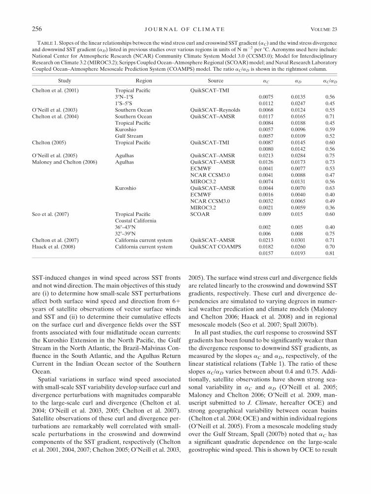
In all past studies, the curl response to crosswind SST

gradients has been found to be significantly weaker than

the divergence response to downwind SST gradients, as

measured by the slopes aC and aD, respectively, of the

linear statistical relations (Table 1). The ratio of these

slopes aC/aD varies between about 0.4 and 0.75. Addi-

tionally, satellite observations have shown strong sea-

sonal variability in aC and aD (O’Neill et al. 2005;

Maloney and Chelton 2006; O’Neill et al. 2009, man-

uscript submitted to J. Climate, hereafter OCE) and

strong geographical variability between ocean basins

(Chelton et al. 2004; OCE) and within individual regions

(O’Neill et al. 2005). From a mesoscale modeling study

over the Gulf Stream, Spall (2007b) noted that aC has

a significant quadratic dependence on the large-scale

geostrophic wind speed. This is shown by OCE to result

TABLE 1. Slopes of the linear relationships between the wind stress curl and crosswind SST gradient (aC) and the wind stress divergence

and downwind SST gradient (aD) listed in previous studies over various regions in units of N m22 per 8C. Acronyms used here include:

National Center for Atmospheric Research (NCAR) Community Climate System Model 3.0 (CCSM3.0); Model for Interdisciplinary

Research on Climate 3.2 (MIROC3.2); Scripps Coupled Ocean–Atmosphere Regional (SCOAR) model; and Naval Research Laboratory

Coupled Ocean–Atmosphere Mesoscale Prediction System (COAMPS) model. The ratio aC/aD is shown in the rightmost column.

Study Region Source aC aD aC/aD

Chelton et al. (2001) Tropical Pacific QuikSCAT–TMI

38N–18S 0.0075 0.0135 0.56

18S–58S 0.0112 0.0247 0.45

O’Neill et al. (2003) Southern Ocean QuikSCAT–Reynolds 0.0068 0.0124 0.55

Chelton et al. (2004) Southern Ocean QuikSCAT–AMSR 0.0117 0.0165 0.71

Tropical Pacific 0.0084 0.0188 0.45

Kuroshio 0.0057 0.0096 0.59

Gulf Stream 0.0057 0.0109 0.52

Chelton (2005) Tropical Pacific QuikSCAT–TMI 0.0087 0.0145 0.60

0.0080 0.0142 0.56

O’Neill et al. (2005) Agulhas QuikSCAT–AMSR 0.0213 0.0284 0.75

Maloney and Chelton (2006) Agulhas QuikSCAT–AMSR 0.0126 0.0173 0.73

ECMWF 0.0041 0.0077 0.53

NCAR CCSM3.0 0.0041 0.0088 0.47

MIROC3.2 0.0074 0.0131 0.56

Kuroshio QuikSCAT–AMSR 0.0044 0.0070 0.63

ECMWF 0.0016 0.0040 0.40

NCAR CCSM3.0 0.0032 0.0065 0.49

MIROC3.2 0.0021 0.0059 0.36

Seo et al. (2007) Tropical Pacific SCOAR 0.009 0.015 0.60

Coastal California

368–438N 0.002 0.005 0.40

328–398N 0.006 0.008 0.75

Chelton et al. (2007) California current system QuikSCAT–AMSR 0.0213 0.0301 0.71

Haack et al. (2008) California current system QuikSCAT COAMPS 0.0182 0.0260 0.70

0.0157 0.0193 0.81

256 J O U R N A L O F C L I M A T E VOLUME 23

from the nonlinearity between SST-induced surface wind

speed and wind stress perturbations.

Beyond what is known about the dynamics of the

near-surface wind response to small-scale SST pertur-

bations, as discussed in section 2, little is known about

the dynamics underlying the curl and divergence re-

sponses to SST gradients. The differences in the curl and

divergence responses reveal an opportunity to better

understand how the marine atmospheric boundary layer

(MABL) responds to small-scale SST perturbations.

In this study, surface wind speed and direction are

obtained from the SeaWinds scatterometer onboard the

Quick Scatterometer (QuikSCAT) satellite and SST is

obtained from the Advanced Microwave Scanning Ra-

diometer for Earth Observing System (EOS) (AMSR-E)

Aqua satellite, as discussed in section 3. The statistical

responses of spatially high-pass filtered surface wind

speed and direction as functions of SST are shown in

section 4. A relatively simple statistical relation is found

between surface wind speed and SST despite the com-

plicated force balances involved in the SST-induced

MABL response described by previous studies. In sec-

tion 5, the QuikSCAT vorticity and divergence of the

surface wind field are shown to depend on the crosswind

and downwind SST gradients in a manner analogous to

the dependencies of the wind stress curl and divergence

considered in our previous studies. While the vorticity

and divergence responses to SST gradients have been

interpreted previously in terms of SST effects on surface

wind stress magnitude (or wind speed), we show that

SST also modifies the surface wind direction, thus also

contributing to SST-induced changes in the surface

vorticity and divergence. These SST-induced modifica-

tions of wind direction are shown to be responsible for

the differing vorticity and divergence responses to SST.

We close in section 6 with a discussion of the implica-

tions of the results of this study for coupled mesoscale

wind–SST interactions.

2. Dynamical explanations for mesoscalewind–SST coupling

Many observational and modeling studies have now

been undertaken to better understand the MABL re-

sponse to SST perturbations over various regions of the

World Ocean. The response of surface winds to meso-

scale SST perturbations is the culmination of adjustment

processes extending throughout the depth of the MABL

and appears to be controlled mainly by modification of

the surface heat fluxes as air flows across SST fronts.

Surface heat fluxes are enhanced or suppressed depend-

ing on whether the flow is from cold to warm water or

vice versa. Cross-frontal surface heating perturbations

produce changes in the MABL hydrostatic pressure

gradients and to the vertical turbulent stress divergence

in the MABL as described below, ultimately leading to

changes in near-surface winds coupled to the mesoscale

SST perturbations.

Across SST fronts, variations in surface heating cause

cross-frontal pressure gradients near the surface since

a cooler MABL over cooler water forms higher surface

pressures relative to a warmer MABL over warmer

water. Thermally induced pressure gradients so formed

can therefore accelerate near-surface flow across SST

isotherms from cooler to warmer water and vice versa.

Using an analytical model of the boundary layer,

Lindzen and Nigam (1987) attributed acceleration of

cross-equatorial surface flow north of the equatorial cold

tongue in the eastern tropical Pacific primarily to ther-

mally induced pressure gradients associated with the cold

tongue meridional SST gradient. Even though some of

the assumptions of their analytical model are not gener-

ally valid (e.g., Battisti et al. 1999; Stevens et al. 2002;

Small et al. 2003), SST-induced pressure gradients are

indeed strong contributors to the SST-induced surface

wind response (e.g., Wai and Stage 1989; Warner et al.

1990; Small et al. 2003; Cronin et al. 2003; Mahrt et al.

2004; Bourras et al. 2004; Song et al. 2004; Small et al. 2005b;

Song et al. 2006). Using mesoscale numerical simula-

tions over the equatorial Pacific, Small et al. (2003)

showed that near-surface pressure perturbations form

in response to SST-induced MABL air temperature var-

iations, which are governed thermodynamically by a bal-

ance between horizontal temperature advection and

surface sensible heat fluxes. From surface pressure obser-

vations over the equatorial Pacific, Cronin et al. (2003)

have shown that SST-induced surface pressure gradient

perturbations associated with the northern equatorial

cold tongue are of a magnitude similar to those gener-

ated by mesoscale model simulations. Hashizume et al.

(2002) have also suggested that deepening and shoaling

of the MABL associated with cross-frontal turbulent

mixing variations counteracts this thermodynamic con-

tribution to the SST-induced surface pressure variations

in what has been referred to as a ‘‘backpressure’’ effect.

Finally, while MABL pressure gradients contribute to

near-surface flow acceleration perpendicular to SST

isotherms, it is not clear how they contribute to the

generation of near-surface vorticity as air blows parallel

to SST isotherms, a feature generally observed in scat-

terometer wind fields globally.

Wallace et al. (1989) and Hayes et al. (1989) argued

that vertical turbulent mixing of momentum from aloft

to the surface was more consistent with the changes in

vertical wind shear and the acceleration of surface winds

occurring across the northern edge of the equatorial

15 JANUARY 2010 O ’ N E I L L E T A L . 257

Pacific cold tongue than with thermally induced pressure

gradients. Earlier aircraft observations over the north

wall of the Gulf Stream by Sweet et al. (1981) also showed

that turbulent mixing of momentum from aloft to the

surface also played a significant role in near-surface wind

speed variations. With this mechanism, SST-induced sur-

face heating modifies the static stability of the boundary

layer, enhancing the vertical turbulent mixing of momen-

tum as air blows from cool to warm water and reducing

it as air blows from warm to cool water. Observations

of the near-surface vertical turbulent momentum flux

throughout the world’s oceans have generally shown con-

siderable variation upon crossing SST fronts and have

supported this hypothesis (Mey and Walker 1990; Freihe

et al. 1991; Bond 1992; Jury 1994; Rouault and Lutjeharms

2000; Mahrt et al. 2004; de Szoeke et al. 2005; Tokinaga

et al. 2006).

Modeling studies of the surface wind response to me-

soscale SST perturbations have been less consistent

about the role that the vertical turbulent stress divergence

plays in the SST-induced surface wind response. Some

investigators find a significant role (Wai and Stage 1989;

de Szoeke and Bretherton 2004; Bourras et al. 2004;

Song et al. 2004; Skyllingstad et al. 2006; Thum 2006;

Song et al. 2009; O’Neill et al. 2010) while others found

less significant roles (Small et al. 2003; Bourras et al.

2004; Small et al. 2005a,b; Song et al. 2006; Samelson

et al. 2006; Spall 2007b). Additionally, the contribution

of surface ocean currents to the surface stress may play

a small but nonnegligible role in the near-surface verti-

cal turbulent stress divergence (Song et al. 2006; Liu

et al. 2007). Idealized large-eddy simulations of the flow

across sharp SST fronts by Skyllingstad et al. (2006)

showed that on spatial scales of 1–20 km, which are

somewhat smaller than considered here, near-surface

wind speed variations are influenced predominantly by

SST-induced cross-frontal variations in the vertical tur-

bulent mixing of momentum, consistent with the Wallace

et al. (1989) and Hayes et al. (1989) hypotheses. Finally,

weak coupling of surface winds to SST in the European

Centre for Medium-Range Weather Forecasts (ECMWF)

model over the Agulhas Return Current (Maloney and

Chelton 2006) was shown by Song et al. (2009) to be

attributable primarily to a weak response of the pa-

rameterized vertical turbulent stress divergence to SST-

induced surface heating perturbations.

Small et al. (2005a) envisioned a quite different role of

the vertical turbulent stress divergence in a numerical

simulation of the near-surface wind response over the

eastern tropical Pacific. There, it was found that pressure

gradients accelerated the near-surface flow across the

cold tongue SST front, and after some distance, the

vertical turbulent stress divergence acted as a frictional

drag on this pressure-driven flow. In this ‘‘pressure-drag’’

mechanism, turbulence acts to reduce the surface winds

in an opposite manner to that hypothesized by Wallace

et al. (1989) and Hayes et al. (1989). This pressure-drag

mechanism was found to operate in a numerical simu-

lation over the Agulhas Return Current (O’Neill et al.

2010), but only above about 150 m from the surface;

below this level, the near-surface winds were influenced by

the turbulent mixing of momentum in accordance with the

Wallace et al. (1989) and Hayes et al. (1989) mechanism.

Samelson et al. (2006) argued that changes in boundary

layer depth somewhat downwind of the sharpest SST

gradients, rather than the vertical redistribution of mo-

mentum, could act to change the surface stress. This

mechanism acts through a balance of a fixed large-scale

pressure gradient and the vertical turbulent stress di-

vergence integrated vertically over the depth of the

boundary layer such that the ratio of surface stress to

boundary layer height t/H is equal to a fixed large-scale

pressure gradient integrated over the depth of the bound-

ary layer. This balance was found to be consistent with

the cross-frontal changes in surface stress and boundary

layer height away from the steepest SST gradients in

the two-dimensional model simulation of Spall (2007b).

This balance assumes that the SST-induced responses of

the vertical turbulent mixing of momentum, thermally

induced pressure gradients, and horizontal advection

are not significant terms in the MABL momentum bud-

get in regions directly over the sharpest SST fronts (see

detailed discussion in Small et al. 2008).

At midlatitudes, Coriolis accelerations have been

shown to be important to the response of the surface

winds to small-scale SST perturbations (e.g., Wai and

Stage 1989; Bourras et al. 2004; Thum 2006; Song et al.

2006; Spall 2007b; O’Neill et al. 2010). Over a single SST

front, Spall (2007b) has found that SST-induced turbu-

lent mixing perturbations induce Coriolis accelerations

analogous to an inertially driven lee wave. O’Neill et al.

(2010) has found evidence of a similar mechanism in

a simulation over a part of the Southern Ocean. The

strong large-scale mean wind speeds typically found

over midlatitude ocean fronts also lead to significant

horizontal advective accelerations that strongly influ-

ence the near-surface momentum budget (Song et al.

2006; Thum 2006; Spall 2007b; O’Neill et al. 2010).

Some debate remains as to the physical mechanisms

involved in the coupling between surface winds and

mesoscale SST perturbations. It is becoming clear, how-

ever, that both pressure gradients and the turbulent

mixing of momentum are involved significantly in the

response. There are also likely significant regional dif-

ferences in the large-scale atmospheric forcing that may

alter the force balance involved in the surface wind

258 J O U R N A L O F C L I M A T E VOLUME 23

response. We show below that there are comparatively

simple statistical relationships between the surface winds

and SST despite the rather complicated details of these

physical mechanisms.

3. Description of satellite observations and methods

This study utilizes monthly-averaged surface vector

wind observations from the QuikSCAT scatterometer

and SST from the AMSR-E over the 75-month period

June 2002–August 2008, coinciding with the first 61

years of the AMSR-E geophysical observational data

record that began 1 June 2002. Each of these datasets is

summarized in this section.

a. QuikSCAT wind fields

In nonprecipitating conditions, scatterometers infer

surface vector winds over water from microwave radar

measurements of small-scale surface roughness caused

by surface wind stress. For lack of abundant direct sur-

face stress measurements, scatterometer measurements

of microwave radar backscatter are calibrated to buoy

anemometer measurements of the so-called equivalent

neutral stability wind at 10 m, which is the 10-m wind

that would be uniquely related to the observed surface

wind stress if the atmosphere were neutrally stratified

(Liu and Tang 1996). The relation between the equiva-

lent neutral stability wind vector u and the surface wind

stress vector t is t 5 r0CDNVu, where r0 is the surface air

density, V is the magnitude of u, and CDN is the neutral

stability drag coefficient.

The computations throughout this paper using

QuikSCAT winds are based on 10-m equivalent neutral

stability winds. On average, anemometer measurements

of the 10-m wind speed are about 0.2 m s21 lower than

the corresponding neutral-stability wind speed at 10 m

(Mears et al. 2001; see also Fig. 16 of Chelton and

Freilich 2005) because the atmospheric surface layer is,

on average, slightly unstable over all oceans. Through

comparisons with high-quality buoy anemometer mea-

surements, QuikSCAT wind speed measurement errors

have been estimated to be about 1.7 m s21 (Chelton and

Freilich 2005). The wind direction accuracy improves

with increasing wind speed; for wind speeds greater than

about 5 m s21, the direction accuracy of individual wind

measurements is better than 158 (see Fig. 8 in Chelton

and Freilich 2005). Additionally, there is no evidence of

SST-dependent measurement biases in the QuikSCAT

wind observations (Chelton et al. 2001; Ebuchi et al.

2002).

The spatial derivatives of wind components, wind

speed, and wind direction analyzed in this study were

computed ‘‘in-swath’’ before interpolating to a regular

spatial grid. This avoids complications arising from the

estimation of spatial derivatives near swath edges where

centered first-difference estimates of derivatives are com-

puted using measurements from neighboring swaths sep-

arated in time by several hours or more. The various wind

and derivative wind fields of interest in this study were

then constructed on a 0.258 latitude by 0.258 longitude

spatial grid by fitting in-swath measurements to a qua-

dratic surface using locally weighted regression (‘‘loess’’

smoothing; Cleveland and Devlin 1988) with a half span of

80 km. Based on the filter transfer function of the loess

smoother (Schlax et al. 2001; Chelton and Schlax 2003),

the resulting gridded fields have a spatial resolution

analogous to that of approximately 50-km block averages.

The spatial derivative fields were found at each grid point

directly from the regression coefficients of the quadratic

surface. The wind fields were then averaged at monthly

intervals from the gridded swath data.

b. AMSR-E SST fields

The detailed results of this study would not be possible

without the near-all-weather microwave observations of

SST over middle- and high-latitude regions provided by

the AMSR-E since June 2002 (Chelton and Wentz 2005).

The main advantage of microwave measurements of SST

is the ability to measure SST through nonprecipitating

clouds, which are essentially transparent to microwave

radiation. Cloud cover generally obscures the midlat-

itude ocean regions of interest in this study more than

70% of the time (Chelton and Wentz 2005). Large re-

gions of missing data often occur in SST fields con-

structed from infrared satellite measurements over the

sharpest ocean fronts and eddies where strong ocean–

atmosphere interactions are expected to occur (see, e.g.,

Fig. 6 of Chelton and Wentz 2005). Indeed, stratocu-

mulus and cumulus cloud bands often form over sharp

SST fronts as a consequence of some of the same MABL

adjustment processes affecting MABL winds of inter-

est in this study (e.g., Norris and Iacobellis 2005). While

SST measurements by the Tropical Rainfall Measuring

Mission (TRMM) Microwave Imager (TMI) have been

available since December 1997 and thus encompass the

entire QuikSCAT mission, they are only made equator-

ward of 408 latitude, leaving most of the midlatitude re-

gions of interest in this analysis unsampled.

The AMSR-E measures horizontally and vertically

polarized brightness temperatures at six microwave

frequencies across a 1450-km swath. From these 12 mi-

crowave brightness temperatures, SST is estimated over

most of the global oceans using a physically based statis-

tical regression algorithm (Wentz and Meissner 2000). The

footprint size of AMSR-E measurements of SST is 56 km

and the rms accuracy of individual SST measurements is

15 JANUARY 2010 O ’ N E I L L E T A L . 259

about 0.48C (Chelton and Wentz 2005). The SST fields

were gridded onto the same 0.258 grid as the QuikSCAT

surface wind fields and then averaged at monthly in-

tervals.

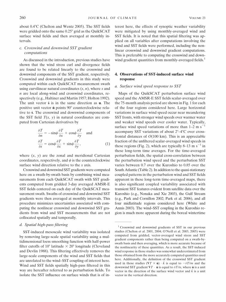
c. Crosswind and downwind SST gradientcomputations

As discussed in the introduction, previous studies have

shown that the wind stress curl and divergence fields

are found to be related linearly to the crosswind and

downwind components of the SST gradient, respectively.

Crosswind and downwind gradients in this study were

computed within each QuikSCAT measurement swath

using curvilinear natural coordinates (s, n), where s and

n are local along-wind and crosswind coordinates, re-

spectively (e.g., Haltiner and Martin 1957; Holton 1992).

The unit vector s is in the same direction as u. The

positive unit vector n points 908 counterclockwise rela-

tive to s. The crosswind and downwind components of

the SST field T(x, y) in natural coordinates are com-

puted from Cartesian derivatives by

›T

›n5�sinc

›T

›x1 cosc

›T

›yand

›T

›s5 cosc

›T

›x1 sinc

›T

›y, (1)

where (x, y) are the zonal and meridional Cartesian

coordinates, respectively, and c is the counterclockwise

surface wind direction relative to the x axis.

Crosswind and downwind SST gradients were computed

here on a swath-by-swath basis by combining wind mea-

surements from each QuikSCAT swath with SST gradi-

ents computed from gridded 3-day averaged AMSR-E

SST fields centered on each day of the QuikSCAT mea-

surement swath. Swaths of crosswind and downwind SST

gradients were then averaged at monthly intervals. This

procedure minimizes uncertainties associated with com-

puting the nonlinear crosswind and downwind SST gra-

dients from wind and SST measurements that are not

collocated spatially and temporally.

d. Spatial high-pass filtering

SST-induced mesoscale wind variability was isolated

by removing large-scale spatial variability using a mul-

tidimensional loess smoothing function with half-power

filter cutoffs of 108 latitude 3 208 longitude (Cleveland

and Devlin 1988). This filtering effectively removes the

large-scale components of the wind and SST fields that

are unrelated to the wind–SST coupling of interest here.

Wind and SST fields spatially high-pass filtered in this

way are hereafter referred to as perturbation fields. To

isolate the SST influence on surface winds that is of in-

terest here, the effects of synoptic weather variability

were mitigated by using monthly-averaged wind and

SST fields. It is noted that this spatial filtering was ap-

plied on all variables after computations involving the

wind and SST fields were performed, including the non-

linear crosswind and downwind gradient computations.

This is preferable to computing the crosswind and down-

wind gradient quantities from monthly-averaged fields.1

4. Observations of SST-induced surface windresponse

a. Surface wind speed response to SST

Maps of the QuikSCAT perturbation surface wind

speed and the AMSR-E SST fields scalar-averaged over

the 75-month analysis period are shown in Fig. 1 for each

of the four regions considered here. Large horizontal

variations in surface wind speed occur near meandering

SST fronts, with stronger wind speeds over warmer water

and weaker wind speeds over cooler water. Typically,

surface wind speed variations of more than 1–2 m s21

accompany SST variations of about 28–48C over cross-

frontal distances of O(100 km). This is an appreciable

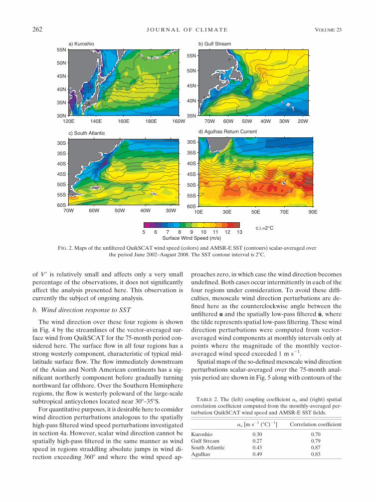
fraction of the unfiltered scalar-averaged wind speeds in

these regions (Fig. 2), which are typically 8–13 m s21 in

these long-term time averages. For the time-averaged

perturbation fields, the spatial cross-correlation between

the perturbation wind speed and the perturbation SST

varies between 0.7 over the Kuroshio to 0.85 over the

South Atlantic (Table 2). In addition to the quasi-stationary

coupled patterns in the perturbation wind and SST fields

apparent in these long-term time-averaged maps, there

is also significant coupled variability associated with

transient SST features evident from satellite data over the

Kuroshio (e.g., Nonaka and Xie 2003), the Gulf Stream

(e.g., Park and Cornillon 2002; Park et al. 2006), and all

four midlatitude regions considered here (White and

Annis 2003). The wind–SST coupling in the Kuroshio re-

gion is much more apparent during the boreal wintertime

1 Crosswind and downwind gradients of SST in our previous

studies (Chelton et al. 2001, 2004; O’Neill et al. 2003, 2005) were

computed from gridded, vector-averaged wind stress and SST

gradient components rather than being computed on a swath-by-

swath basis and then averaging, which is more accurate because of

the nonlinearity of these quantities. As a result, the SST-induced

wind response in those studies was somewhat underestimated from

those obtained from the more accurately computed quantities used

here. Additionally, the definition of the crosswind SST gradient

used in those studies ($T 3 u) � k is equal to 2›T/›n and the

downwind SST gradient $T � u is equal to ›T/›s, where u is a unit

vector in the direction of the surface wind vector and k is a unit

vector in the vertical direction.

260 J O U R N A L O F C L I M A T E VOLUME 23

(e.g., Nonaka and Xie 2003; OCE) and is associated with

strong seasonality of the SST fronts in this region (e.g.,

Nonaka and Xie 2003).

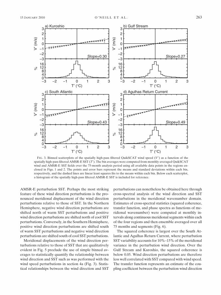
The mesoscale response of the wind speed to SST is

quantified statistically by bin-averaging monthly averages

of the perturbation QuikSCAT wind speed as a function

of the perturbation AMSR-E SST over the 75-month

analysis period (Fig. 3). Wind speed perturbations are

related linearly to, and correlated positively with, me-

soscale SST perturbations over all four regions. The

relationship between the monthly-averaged spatially high-

pass filtered wind speed V9 and SST T9 can thus be ex-

pressed empirically as

V9 5 ayT9, (2)

where ay is the least squares estimate of the slope of

these linear relations and represents the change in wind

speed per unit change in SST (i.e., ay 5 ›V9/›T9) and the

primes hereafter represent spatially high-pass filtered

fields. Notably, ay varies by nearly a factor of 2 geo-

graphically, from 0.27 m s21 per 8C over the Gulf Stream

to 0.49 m s21 per 8C over the Agulhas Return Current

(see Table 2). Additionally, ay is much larger in the two

Southern Hemisphere regions compared to those in the

Northern Hemisphere. The larger error bars at large

perturbation SST magnitudes in Fig. 3 are due to the

smaller numbers of samples in these bins. This is par-

ticularly acute over the Kuroshio, where the monthly-

averaged SST perturbations tend, on average, to be

smaller in magnitude than in the other three regions.

The geographical differences in ay between the four

regions are likely due to geographic differences in the

vertical structure of the boundary layer and large-scale

forcing. Seasonality of ay is investigated from 51 years

of satellite data over these four regions (and the eastern

tropical Pacific) in OCE.

Finally, we note that for SST perturbations warmer

than about 1.58, there is a subtle flattening of the bin-

averaged V9 relative to the linear fit, particularly over

the South Atlantic and Agulhas Return Current regions.

Interestingly, this flattening does not occur over cool

SST perturbations. This difference between the bin-

averaged V9 and the linear fit is less than about 0.25 m s21,

and there are very few data points in these outer bins, as

shown by the histograms in Fig. 3. Because this flattening

FIG. 1. Maps of the perturbation QuikSCAT wind speed (colors) and AMSR-E SST (contours) scalar-averaged

over the period June 2002–August 2008 for the four regions considered in this study. The contour interval for the

perturbation SST is 0.58C, and the zero contour has been omitted for clarity. Solid and dashed contours correspond to

positive and negative values, respectively. The spatial high-pass filter removes spatial variability with wavelengths

longer than 208 longitude 3 108 latitude, as discussed in the text.

15 JANUARY 2010 O ’ N E I L L E T A L . 261

of V9 is relatively small and affects only a very small

percentage of the observations, it does not significantly

affect the analysis presented here. This observation is

currently the subject of ongoing analysis.

b. Wind direction response to SST

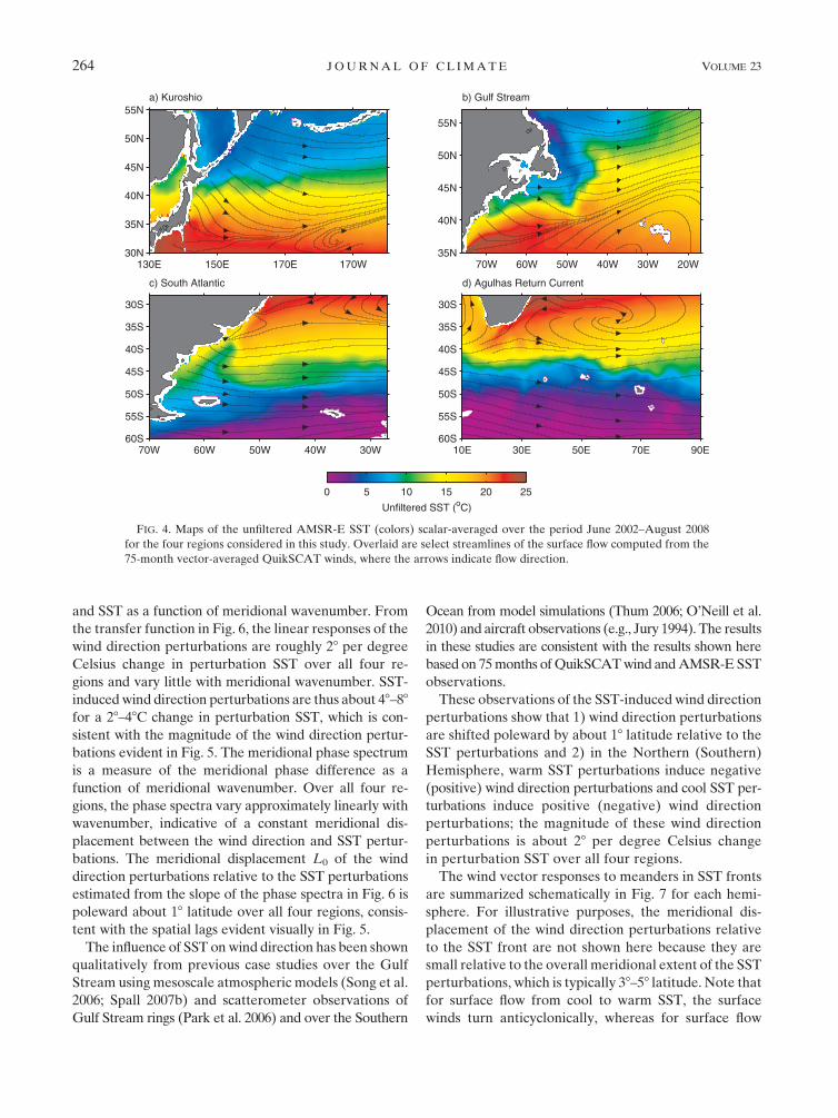
The wind direction over these four regions is shown

in Fig. 4 by the streamlines of the vector-averaged sur-

face wind from QuikSCAT for the 75-month period con-

sidered here. The surface flow in all four regions has a

strong westerly component, characteristic of typical mid-

latitude surface flow. The flow immediately downstream

of the Asian and North American continents has a sig-

nificant northerly component before gradually turning

northward far offshore. Over the Southern Hemisphere

regions, the flow is westerly poleward of the large-scale

subtropical anticyclones located near 308–358S.

For quantitative purposes, it is desirable here to consider

wind direction perturbations analogous to the spatially

high-pass filtered wind speed perturbations investigated

in section 4a. However, scalar wind direction cannot be

spatially high-pass filtered in the same manner as wind

speed in regions straddling absolute jumps in wind di-

rection exceeding 3608 and where the wind speed ap-

proaches zero, in which case the wind direction becomes

undefined. Both cases occur intermittently in each of the

four regions under consideration. To avoid these diffi-

culties, mesoscale wind direction perturbations are de-

fined here as the counterclockwise angle between the

unfiltered u and the spatially low-pass filtered ~u, where

the tilde represents spatial low-pass filtering. These wind

direction perturbations were computed from vector-

averaged wind components at monthly intervals only at

points where the magnitude of the monthly vector-

averaged wind speed exceeded 1 m s21.

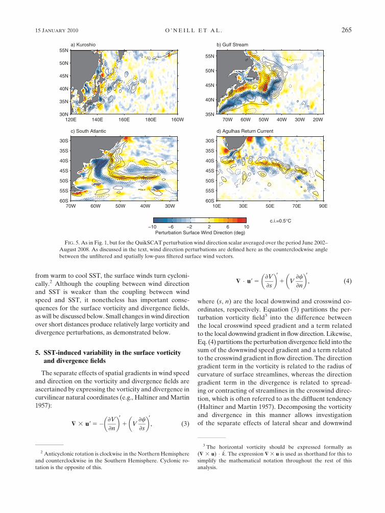
Spatial maps of the so-defined mesoscale wind direction

perturbations scalar-averaged over the 75-month anal-

ysis period are shown in Fig. 5 along with contours of the

FIG. 2. Maps of the unfiltered QuikSCAT wind speed (colors) and AMSR-E SST (contours) scalar-averaged over

the period June 2002–August 2008. The SST contour interval is 28C.

TABLE 2. The (left) coupling coefficient ay and (right) spatial

correlation coefficient computed from the monthly-averaged per-

turbation QuikSCAT wind speed and AMSR-E SST fields.

ay [m s21 (8C)21] Correlation coefficient

Kuroshio 0.30 0.70

Gulf Stream 0.27 0.79

South Atlantic 0.43 0.87

Agulhas 0.49 0.83

262 J O U R N A L O F C L I M A T E VOLUME 23

AMSR-E perturbation SST. Perhaps the most striking

feature of these wind direction perturbations is the pro-

nounced meridional displacement of the wind direction

perturbations relative to those of SST. In the Northern

Hemisphere, negative wind direction perturbations are

shifted north of warm SST perturbations and positive

wind direction perturbations are shifted north of cool SST

perturbations. Conversely, in the Southern Hemisphere,

positive wind direction perturbations are shifted south

of warm SST perturbations and negative wind direction

perturbations are shifted south of cool SST perturbations.

Meridional displacements of the wind direction per-

turbations relative to those of SST that are qualitatively

evident in Fig. 5 preclude the use of simple binned av-

erages to statistically quantify the relationship between

wind direction and SST such as was performed with the

wind speed perturbations in section 4a (Fig. 3). Statis-

tical relationships between the wind direction and SST

perturbations can nonetheless be obtained here through

cross-spectral analysis of the wind direction and SST

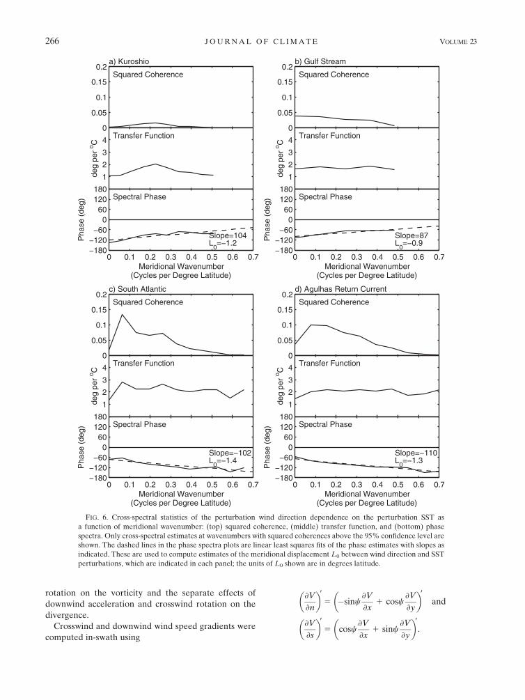
perturbations in the meridional wavenumber domain.

Estimates of cross-spectral statistics (squared coherence,

transfer function, and phase spectra as functions of me-

ridional wavenumber) were computed at monthly in-

tervals along continuous meridional segments within each

of the four regions and then ensemble averaged over all

75 months and segments (Fig. 6).

The squared coherence is largest over the South At-

lantic and Agulhas Return Current, where perturbation

SST variability accounts for 10%–15% of the meridional

variance in the perturbation wind direction. Over the

Gulf Stream and Kuroshio, the squared coherence is

below 0.05. Wind direction perturbations are therefore

less well correlated with SST compared with wind speed.

The transfer function represents an estimate of the cou-

pling coefficient between the perturbation wind direction

FIG. 3. Binned scatterplots of the spatially high-pass filtered QuikSCAT wind speed (V9) as a function of the

spatially high-pass filtered AMSR-E SST (T9). The bin averages were computed from monthly-averaged QuikSCAT

wind and AMSR-E SST fields over the 75-month analysis period using all available data points in the regions en-

closed in Figs. 1 and 2. The points and error bars represent the means and standard deviations within each bin,

respectively, and the dashed lines are linear least squares fits to the means within each bin. Below each scatterplot,

a histogram of the spatially high-pass filtered AMSR-E SST is included for reference.

15 JANUARY 2010 O ’ N E I L L E T A L . 263

and SST as a function of meridional wavenumber. From

the transfer function in Fig. 6, the linear responses of the

wind direction perturbations are roughly 28 per degree

Celsius change in perturbation SST over all four re-

gions and vary little with meridional wavenumber. SST-

induced wind direction perturbations are thus about 48–88

for a 28–48C change in perturbation SST, which is con-

sistent with the magnitude of the wind direction pertur-

bations evident in Fig. 5. The meridional phase spectrum

is a measure of the meridional phase difference as a

function of meridional wavenumber. Over all four re-

gions, the phase spectra vary approximately linearly with

wavenumber, indicative of a constant meridional dis-

placement between the wind direction and SST pertur-

bations. The meridional displacement L0 of the wind

direction perturbations relative to the SST perturbations

estimated from the slope of the phase spectra in Fig. 6 is

poleward about 18 latitude over all four regions, consis-

tent with the spatial lags evident visually in Fig. 5.

The influence of SST on wind direction has been shown

qualitatively from previous case studies over the Gulf

Stream using mesoscale atmospheric models (Song et al.

2006; Spall 2007b) and scatterometer observations of

Gulf Stream rings (Park et al. 2006) and over the Southern

Ocean from model simulations (Thum 2006; O’Neill et al.

2010) and aircraft observations (e.g., Jury 1994). The results

in these studies are consistent with the results shown here

based on 75 months of QuikSCAT wind and AMSR-E SST

observations.

These observations of the SST-induced wind direction

perturbations show that 1) wind direction perturbations

are shifted poleward by about 18 latitude relative to the

SST perturbations and 2) in the Northern (Southern)

Hemisphere, warm SST perturbations induce negative

(positive) wind direction perturbations and cool SST per-

turbations induce positive (negative) wind direction

perturbations; the magnitude of these wind direction

perturbations is about 28 per degree Celsius change

in perturbation SST over all four regions.

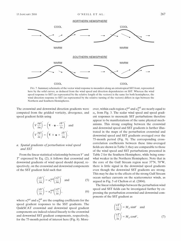
The wind vector responses to meanders in SST fronts

are summarized schematically in Fig. 7 for each hemi-

sphere. For illustrative purposes, the meridional dis-

placement of the wind direction perturbations relative

to the SST front are not shown here because they are

small relative to the overall meridional extent of the SST

perturbations, which is typically 38–58 latitude. Note that

for surface flow from cool to warm SST, the surface

winds turn anticyclonically, whereas for surface flow

FIG. 4. Maps of the unfiltered AMSR-E SST (colors) scalar-averaged over the period June 2002–August 2008

for the four regions considered in this study. Overlaid are select streamlines of the surface flow computed from the

75-month vector-averaged QuikSCAT winds, where the arrows indicate flow direction.

264 J O U R N A L O F C L I M A T E VOLUME 23

from warm to cool SST, the surface winds turn cycloni-

cally.2 Although the coupling between wind direction

and SST is weaker than the coupling between wind

speed and SST, it nonetheless has important conse-

quences for the surface vorticity and divergence fields,

as will be discussed below. Small changes in wind direction

over short distances produce relatively large vorticity and

divergence perturbations, as demonstrated below.

5. SST-induced variability in the surface vorticityand divergence fields

The separate effects of spatial gradients in wind speed

and direction on the vorticity and divergence fields are

ascertained by expressing the vorticity and divergence in

curvilinear natural coordinates (e.g., Haltiner and Martin

1957):

$ 3 u9 5� ›V

›n

� �91 V

›c

›s

� �9, (3)

$ � u9 5›V

›s

� �91 V

›c

›n

� �9, (4)

where (s, n) are the local downwind and crosswind co-

ordinates, respectively. Equation (3) partitions the per-

turbation vorticity field3 into the difference between

the local crosswind speed gradient and a term related

to the local downwind gradient in flow direction. Likewise,

Eq. (4) partitions the perturbation divergence field into the

sum of the downwind speed gradient and a term related

to the crosswind gradient in flow direction. The direction

gradient term in the vorticity is related to the radius of

curvature of surface streamlines, whereas the direction

gradient term in the divergence is related to spread-

ing or contracting of streamlines in the crosswind direc-

tion, which is often referred to as the diffluent tendency

(Haltiner and Martin 1957). Decomposing the vorticity

and divergence in this manner allows investigation

of the separate effects of lateral shear and downwind

FIG. 5. As in Fig. 1, but for the QuikSCAT perturbation wind direction scalar averaged over the period June 2002–

August 2008. As discussed in the text, wind direction perturbations are defined here as the counterclockwise angle

between the unfiltered and spatially low-pass filtered surface wind vectors.

2 Anticyclonic rotation is clockwise in the Northern Hemisphere

and counterclockwise in the Southern Hemisphere. Cyclonic ro-

tation is the opposite of this.

3 The horizontal vorticity should be expressed formally as

($ 3 u) � k. The expression $ 3 u is used as shorthand for this to

simplify the mathematical notation throughout the rest of this

analysis.

15 JANUARY 2010 O ’ N E I L L E T A L . 265

rotation on the vorticity and the separate effects of

downwind acceleration and crosswind rotation on the

divergence.

Crosswind and downwind wind speed gradients were

computed in-swath using

›V

›n

� �95 �sinc

›V

›x1 cosc

›V

›y

� �9

and

›V

›s

� �95 cosc

›V

›x1 sinc

›V

›y

� �9.

FIG. 6. Cross-spectral statistics of the perturbation wind direction dependence on the perturbation SST as

a function of meridional wavenumber: (top) squared coherence, (middle) transfer function, and (bottom) phase

spectra. Only cross-spectral estimates at wavenumbers with squared coherences above the 95% confidence level are

shown. The dashed lines in the phase spectra plots are linear least squares fits of the phase estimates with slopes as

indicated. These are used to compute estimates of the meridional displacement L0 between wind direction and SST

perturbations, which are indicated in each panel; the units of L0 shown are in degrees latitude.

266 J O U R N A L O F C L I M A T E VOLUME 23

The crosswind and downwind direction gradients were

computed from the gridded vorticity, divergence, and

speed gradient fields using

V›c

›n

� �95 $ � u� ›V

›s

� �9

and

V›c

›s

� �95 $ 3 u 1

›V

›n

� �9.

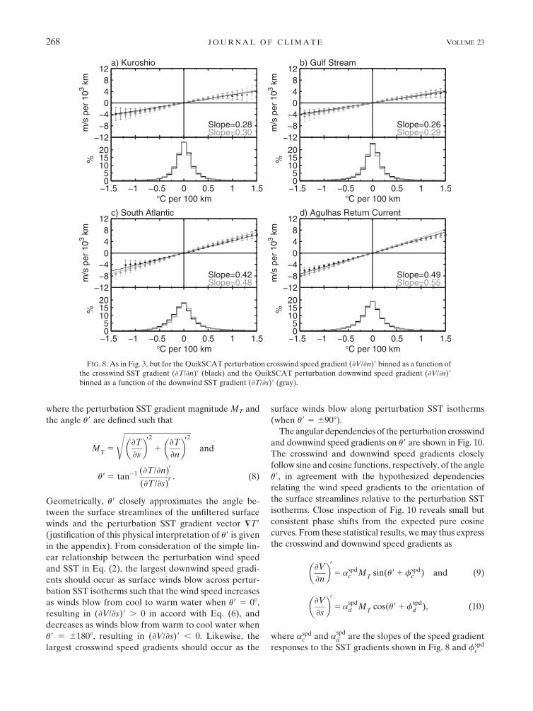
a. Spatial gradients of perturbation wind speedand SST

From the linear statistical relationship between V9 and

T9 expressed by Eq. (2), it follows that crosswind and

downwind gradients of wind speed should depend, re-

spectively, on the crosswind and downwind components

of the SST gradient field such that

›V

›n

� �95 aspd

c

›T

›n

� �9

and (5)

›V

›s

� �95 a

spdd

›T

›s

� �9, (6)

where aspdc and a

spdd are the coupling coefficients for the

speed gradient responses to the SST gradients. The

QuikSCAT crosswind and downwind speed gradient

components are indeed related linearly to the crosswind

and downwind SST gradient components, respectively,

for the 75-month period of interest here (Fig. 8). More-

over, within each region aspdc and a

spdd are nearly equal to

ay from Fig. 3. The scalar wind speed and speed gradi-

ent responses to mesoscale SST perturbations therefore

appear to be manifestations of the same physical mech-

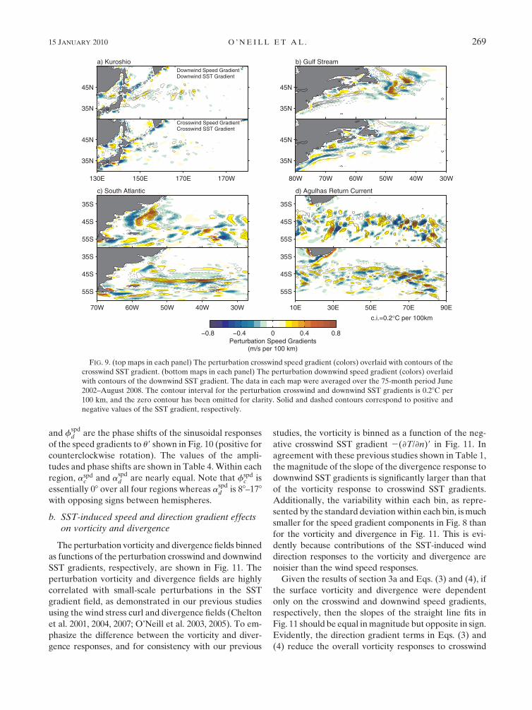
anisms. This strong coupling between the crosswind

and downwind speed and SST gradients is further illus-

trated in the maps of the perturbation crosswind and

downwind speed and SST gradients averaged over the

75-month period (Fig. 9). The corresponding cross-

correlation coefficients between these time-averaged

fields are shown in Table 3; they are comparable to those

of the wind speed and SST perturbations presented in

Table 2 for the Southern Hemisphere, while being some-

what weaker in the Northern Hemisphere. Note that in

the core of the Gulf Stream region near 378N, 708W,

there is little signal in the downwind speed gradients

even though the downwind SST gradients are strong.

This may be due to the effects of the strong Gulf Stream

ocean surface currents on the scatterometer winds, as

argued in Fig. 5 of Chelton et al. (2004).

The linear relationships between the perturbation wind

speed and SST fields can be investigated further by ex-

pressing the perturbation crosswind and downwind com-

ponents of the SST gradient as

›T

›n

� �95 M

Tsinu9 and

›T

›s

� �95 M

Tcosu9, (7)

FIG. 7. Summary schematic of the vector wind response to meanders along an extratropical SST front, represented

here by the solid curves, as deduced from the wind speed and direction dependencies on SST. Whereas the wind

speed response to SST (as represented by the relative length of the vectors) is the same for both hemispheres, the

wind direction response to SST (as represented by the relative turning of the vectors) differs in sign between the

Northern and Southern Hemispheres.

15 JANUARY 2010 O ’ N E I L L E T A L . 267

where the perturbation SST gradient magnitude MT and

the angle u9 are defined such that

MT

5

ffiffiffiffiffiffiffiffiffiffiffiffiffiffiffiffiffiffiffiffiffiffiffiffiffiffiffiffiffiffiffiffiffiffiffiffi›T

›s

� �92

1›T

›n

� �92

sand

u9 5 tan�1 (›T/›n)9

(›T/›s)9. (8)

Geometrically, u9 closely approximates the angle be-

tween the surface streamlines of the unfiltered surface

winds and the perturbation SST gradient vector $T9

(justification of this physical interpretation of u9 is given

in the appendix). From consideration of the simple lin-

ear relationship between the perturbation wind speed

and SST in Eq. (2), the largest downwind speed gradi-

ents should occur as surface winds blow across pertur-

bation SST isotherms such that the wind speed increases

as winds blow from cool to warm water when u9 5 08,

resulting in (›V/›s)9 . 0 in accord with Eq. (6), and

decreases as winds blow from warm to cool water when

u9 5 61808, resulting in (›V/›s)9 , 0. Likewise, the

largest crosswind speed gradients should occur as the

surface winds blow along perturbation SST isotherms

(when u9 5 6908).

The angular dependencies of the perturbation crosswind

and downwind speed gradients on u9 are shown in Fig. 10.

The crosswind and downwind speed gradients closely

follow sine and cosine functions, respectively, of the angle

u9, in agreement with the hypothesized dependencies

relating the wind speed gradients to the orientation of

the surface streamlines relative to the perturbation SST

isotherms. Close inspection of Fig. 10 reveals small but

consistent phase shifts from the expected pure cosine

curves. From these statistical results, we may thus express

the crosswind and downwind speed gradients as

›V

›n

� �95 aspd

c MT

sin(u9 1 fspdc ) and (9)

›V

›s

� �95 a

spdd M

Tcos(u9 1 f

spdd ), (10)

where aspdc and a

spdd are the slopes of the speed gradient

responses to the SST gradients shown in Fig. 8 and fspdc

FIG. 8. As in Fig. 3, but for the QuikSCAT perturbation crosswind speed gradient (›V/›n)9 binned as a function of

the crosswind SST gradient (›T/›n)9 (black) and the QuikSCAT perturbation downwind speed gradient (›V/›s)9

binned as a function of the downwind SST gradient (›T/›s)9 (gray).

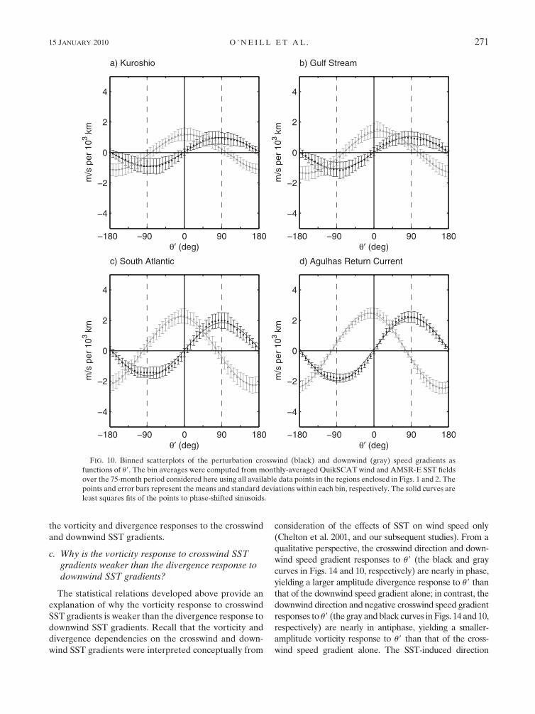
268 J O U R N A L O F C L I M A T E VOLUME 23

and fspdd are the phase shifts of the sinusoidal responses

of the speed gradients to u9 shown in Fig. 10 (positive for

counterclockwise rotation). The values of the ampli-

tudes and phase shifts are shown in Table 4. Within each

region, aspdc and a

spdd are nearly equal. Note that fspd

c is

essentially 08 over all four regions whereas aspdd is 88–178

with opposing signs between hemispheres.

b. SST-induced speed and direction gradient effectson vorticity and divergence

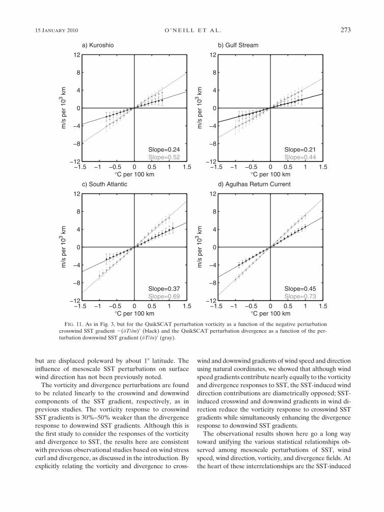
The perturbation vorticity and divergence fields binned

as functions of the perturbation crosswind and downwind

SST gradients, respectively, are shown in Fig. 11. The

perturbation vorticity and divergence fields are highly

correlated with small-scale perturbations in the SST

gradient field, as demonstrated in our previous studies

using the wind stress curl and divergence fields (Chelton

et al. 2001, 2004, 2007; O’Neill et al. 2003, 2005). To em-

phasize the difference between the vorticity and diver-

gence responses, and for consistency with our previous

studies, the vorticity is binned as a function of the neg-

ative crosswind SST gradient 2(›T/›n)9 in Fig. 11. In

agreement with these previous studies shown in Table 1,

the magnitude of the slope of the divergence response to

downwind SST gradients is significantly larger than that

of the vorticity response to crosswind SST gradients.

Additionally, the variability within each bin, as repre-

sented by the standard deviation within each bin, is much

smaller for the speed gradient components in Fig. 8 than

for the vorticity and divergence in Fig. 11. This is evi-

dently because contributions of the SST-induced wind

direction responses to the vorticity and divergence are

noisier than the wind speed responses.

Given the results of section 3a and Eqs. (3) and (4), if

the surface vorticity and divergence were dependent

only on the crosswind and downwind speed gradients,

respectively, then the slopes of the straight line fits in

Fig. 11 should be equal in magnitude but opposite in sign.

Evidently, the direction gradient terms in Eqs. (3) and

(4) reduce the overall vorticity responses to crosswind

FIG. 9. (top maps in each panel) The perturbation crosswind speed gradient (colors) overlaid with contours of the

crosswind SST gradient. (bottom maps in each panel) The perturbation downwind speed gradient (colors) overlaid

with contours of the downwind SST gradient. The data in each map were averaged over the 75-month period June

2002–August 2008. The contour interval for the perturbation crosswind and downwind SST gradients is 0.28C per

100 km, and the zero contour has been omitted for clarity. Solid and dashed contours correspond to positive and

negative values of the SST gradient, respectively.

15 JANUARY 2010 O ’ N E I L L E T A L . 269

SST gradients and enhance the divergence responses to

downwind SST gradients. This point is addressed in de-

tail in section 4c.

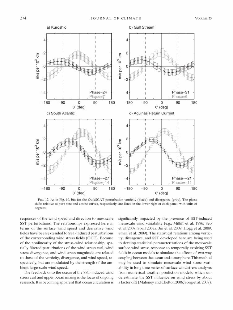
Besides these differences, there are significant differ-

ences in the vorticity and divergence dependencies on u9

(Fig. 12) from that expected solely from consideration of

SST-induced wind speed perturbations. In our previous

work, we hypothesized that the surface curl should de-

pend on the sine of u9 whereas the divergence should

depend on the cosine of u9. Inspection of the vorticity

and divergence dependencies on u9 in Fig. 12, however,

reveals that the vorticity and divergence do not depend

exactly on the sine and cosine, respectively, of u9 but

rather are phase shifted (Fig. 12). The values of the

phase shifts are labeled on Fig. 12. These phase shifts

have absolute magnitudes of approximately 258 for the

vorticity and 108 for the divergence in all four regions

but with opposite signs in each hemisphere. As addressed

below, these phase shifts and the amplitude differences in

Fig. 11 (also evident from the amplitudes of the sinusoids

in Fig. 12) can be related directly to the influence of SST

on the direction gradient terms in Eqs. (3) and (4).

The dependence of the direction gradient terms on

SST can be ascertained conceptually from the schematic

in Fig. 7. When the surface flow is from cool to warm

SST, the surface winds turn anticyclonically, whereas for

surface flow from warm to cool SST the surface winds

turn cyclonically. This observation suggests that the

downwind gradient in wind direction V(›c/›s) should

depend on the downwind SST gradient and hence on the

cosine of u9. Additionally, crosswind direction gradients

V(›c/›n) should form as the wind blows along pertur-

bation SST isotherms in association with the crosswind

SST gradient and will thus depend on the sine of u9.

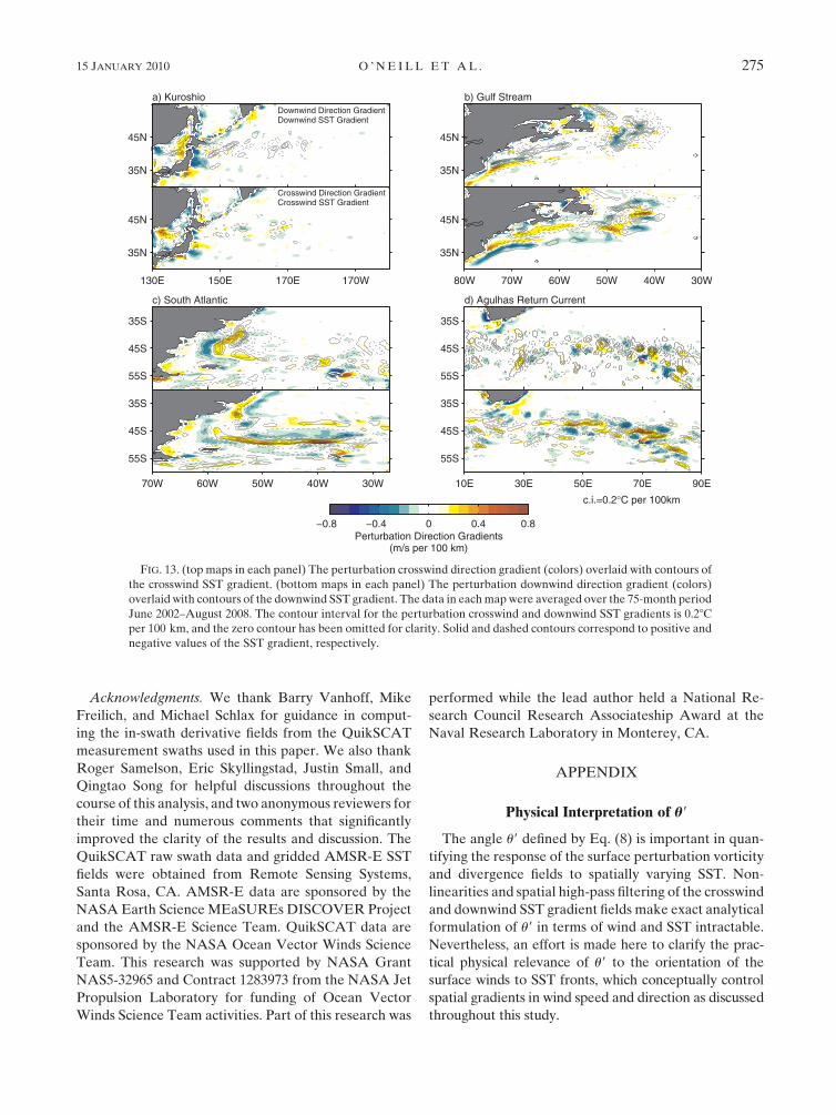
The time-averaged maps of the perturbation downwind

direction and SST gradients and the perturbation cross-

wind direction and SST gradients in Fig. 13 indeed show

a correlation between the direction gradient and SST

gradients consistent with these hypothesized dependen-

cies. The poleward displacement of the wind direction

perturbations relative to those of SST discussed in section

4b is also evident in these maps. The correlations are

weakest over the Kuroshio and strongest in the Southern

Hemisphere regions, as quantified by the cross-correlation

coefficients between the crosswind and downwind di-

rection gradients and the crosswind and downwind SST

gradients, respectively, in Table 3. Additionally, the

magnitudes of the correlation coefficients between the

downwind direction gradients and the downwind SST

gradients are consistently smaller than those between

the crosswind direction gradients and the crosswind SST

gradients. However, both are much smaller than the

correlations between the crosswind and downwind gra-

dients of wind speed and SST, thus explaining the higher

variability of the vorticity and divergence binned aver-

ages in Fig. 11 compared with the speed-only contribu-

tions to the vorticity and divergence in Fig. 8.

The dependencies of the direction gradient terms on

u9 quantified statistically in Fig. 14 confirm that the

crosswind and downwind direction gradients vary as the

sine and cosine of u9, respectively. As expected in all

four regions, the downwind direction gradient response

to u9 (gray curve in Fig. 14) shows that the surface wind

tends to rotate anticyclonically when the large-scale flow

is from cool to warm water (i.e., when u9 5 08) and cy-

clonically when the large-scale flow is from warm to cool

water (i.e., when u9 5 61808). The crosswind direction

gradient response to u9 indicates a maximum surface

diffluent tendency as winds blow approximately along

perturbation SST isotherms (i.e., when u9 5 6908).

Statistically, the direction gradient terms can thus be

represented by

V›c

›s

� �95 adir

d MT

cos(u9� fdird ) and (11)

V›c

›n

� �95 adir

c MT

sin(u9 1 fdirc ), (12)

where adird and adir

c are coupling coefficients for the

downwind and crosswind direction gradients, respectively,

and fdird and fdir

c are phase shifts (see Table 4). These

statistical relations, along with the statistical relations for

the speed gradients in Eqs. (9) and (10), are used in sec-

tion 4c to aid in understanding the differences between

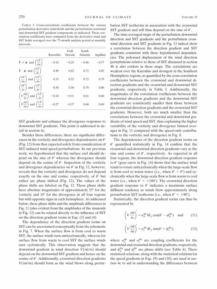
TABLE 3. Cross-correlation coefficients between the various

perturbation derivative wind fields and the perturbation crosswind

and downwind SST gradient components as indicated. These cor-

relation coefficients were computed from the derivative wind and

SST fields averaged over the 75-month analysis period at monthly

intervals.

Kuroshio

Gulf

Stream

South

Atlantic Agulhas

$ 3 u9 and›T

›n

� �9

20.16 20.25 20.46 20.57

$ � u9 and›T

›s

� �9

0.49 0.62 0.72 0.82

›V

›n

� �9

and›T

›n

� �9

0.33 0.52 0.72 0.79

›V

›s

� �9

and›T

›s

� �9

0.50 0.56 0.79 0.86

V›c

›s

� �9

and›T

›s

� �9

20.18 20.31 0.61 0.60

V›c

›n

� �9

and›T

›n

� �9

20.27 20.37 0.68 0.69

270 J O U R N A L O F C L I M A T E VOLUME 23

the vorticity and divergence responses to the crosswind

and downwind SST gradients.

c. Why is the vorticity response to crosswind SSTgradients weaker than the divergence response todownwind SST gradients?

The statistical relations developed above provide an

explanation of why the vorticity response to crosswind

SST gradients is weaker than the divergence response to

downwind SST gradients. Recall that the vorticity and

divergence dependencies on the crosswind and down-

wind SST gradients were interpreted conceptually from

consideration of the effects of SST on wind speed only

(Chelton et al. 2001, and our subsequent studies). From a

qualitative perspective, the crosswind direction and down-

wind speed gradient responses to u9 (the black and gray

curves in Figs. 14 and 10, respectively) are nearly in phase,

yielding a larger amplitude divergence response to u9 than

that of the downwind speed gradient alone; in contrast, the

downwind direction and negative crosswind speed gradient

responses to u9 (the gray and black curves in Figs. 14 and 10,

respectively) are nearly in antiphase, yielding a smaller-

amplitude vorticity response to u9 than that of the cross-

wind speed gradient alone. The SST-induced direction

FIG. 10. Binned scatterplots of the perturbation crosswind (black) and downwind (gray) speed gradients as

functions of u9. The bin averages were computed from monthly-averaged QuikSCAT wind and AMSR-E SST fields

over the 75-month period considered here using all available data points in the regions enclosed in Figs. 1 and 2. The

points and error bars represent the means and standard deviations within each bin, respectively. The solid curves are

least squares fits of the points to phase-shifted sinusoids.

15 JANUARY 2010 O ’ N E I L L E T A L . 271

gradient perturbations thus enhance the divergence re-

sponse to downwind SST gradients while simultaneously

reducing the vorticity response to crosswind SST gradients.

This result can be shown more rigorously by noting

that the crosswind and downwind speed gradient re-

sponses to u9 (Fig. 10) expressed in Eqs. (9) and (10) and

the crosswind and downwind direction gradient responses

to u9 (Fig. 14) expressed in Eqs. (11) and (12) can be

combined to relate the vorticity and divergence fields to

MT and u9 as

$ 3 u9 5�aspdc M

Tsin(u9 1 fspd

c )|fflfflfflfflfflfflfflfflfflfflfflfflfflfflfflfflfflfflfflffl{zfflfflfflfflfflfflfflfflfflfflfflfflfflfflfflfflfflfflfflffl}Crosswind speed gradient

1 adird M

Tcos(u9� fdir

d )|fflfflfflfflfflfflfflfflfflfflfflfflfflfflfflfflfflffl{zfflfflfflfflfflfflfflfflfflfflfflfflfflfflfflfflfflffl}Downwind direction gradient

, and (13)

$ � u9 5 aspdd M

Tcos(u9 1 f

spdd )|fflfflfflfflfflfflfflfflfflfflfflfflfflfflfflfflfflfflffl{zfflfflfflfflfflfflfflfflfflfflfflfflfflfflfflfflfflfflffl}

Downwind speed gradient

1 adirc M

Tsin(u9 1 fdir

c )|fflfflfflfflfflfflfflfflfflfflfflfflfflfflfflfflffl{zfflfflfflfflfflfflfflfflfflfflfflfflfflfflfflfflffl}Crosswind direction gradient

. (14)

The components of the vorticity and divergence that

each term represents empirically in these equations are

indicated by the underbraces. Using trigonometric iden-

tities and rewriting these equations in terms of the cross-

wind and downwind SST gradients using Eq. (7) yields

$ 3 u9 5 avortc

›T

›n

� �91 avort

d

›T

›s

� �9

and

$ � u9 5 adivd

›T

›s

� �91 adiv

c

›T

›n

� �9,

where the set of coupling coefficients (avortc , avort

d ) and

(adivd , adiv

c ) are defined as

avortc 5�aspd

c cosfspdc 1 adir

d sinfdird , (15)

avortd 5�aspd

c sinfspdc 1 adir

d cosfdird , (16)

adivd 5 a

spdd cosf

spdd 1 adir

c sinfdirc , and (17)

adivc 5�a

spdd sinf

spdd 1 adir

c cosfdirc . (18)

Consider Eq. (15) for avortc , which is the coupling co-

efficient for the vorticity response to the crosswind SST

gradient. Both adird and sinfdir

d are statistically found to

be positive quantities (Table 4) over all four regions.

Therefore, the downwind direction gradients reduce the

vorticity response to crosswind SST gradients by a factor

of adird sinfdir

d . Likewise, from consideration of Eq. (17)

for adivd , the crosswind direction gradients enhance the

divergence response to downwind SST gradients by a

factor of adirc sinfdir

c since adirc and sinfdir

c are both found

statistically to be positive quantities (Table 4) over all

four regions. SST-induced wind direction gradients thus

simultaneously reduce the vorticity response to cross-

wind SST gradients and enhance the divergence re-

sponse to downwind SST gradients.

It is also noted that in coupled ocean–atmosphere

simulations of tropical instability waves, Seo et al. (2007)

and Small et al. (2009) have found that Ekman pumping

anomalies associated with SST-induced wind stress curl

perturbations tend to reduce the wind stress curl relative

to the wind stress divergence perturbations. This ap-

parently occurs because surface ocean currents tend to

be quasi-nondivergent, thus affecting the wind stress

curl more than the wind stress divergence. It is currently

unknown whether similar ocean feedbacks act over

midlatitudes to reduce the vorticity response to cross-

wind SST gradients in addition to the wind direction

effects reported here.

6. Conclusions

Analysis of the differences between the surface vortic-

ity and divergence responses to SST have revealed a sig-

nificant response of the wind direction to mesoscale SST

perturbations in addition to the well-known positive cor-

relation and linear response of the surface wind speed to

SST. Analysis of 75 months of QuikSCAT surface vector

winds and AMSR-E SST observations showed that surface

winds accelerate and turn anticyclonically when the surface

flow is from cool to warm SST and decelerate and turn

cyclonically when the surface flow is from warm to cool

SST, with characteristic wind speed changes of 1–2 m s21

and wind direction changes of 48–88. SST-induced wind

direction perturbations are not collocated with SST per-

turbations, as is the case with the wind speed perturbations,

TABLE 4. Values of the coupling coefficients and phase angles

appearing in Eqs. (13)–(18) computed from the QuikSCAT wind

and AMSR-E SST fields. The units of the coupling coefficients are

in m s21 8C21.

Kuroshio Gulf Stream South Atlantic Agulhas

aspdc 0.28 0.26 0.42 0.49

adird 0.13 0.14 0.19 0.17

fspdc 238 258 18 28

fdird 1418 1468 208 238

avortc 20.24 20.22 20.37 20.45

avortd 20.089 20.090 0.17 0.14

aspdd 0.30 0.29 0.48 0.55

adirc 0.20 0.20 0.31 0.30

fspdd 2118 2178 88 128

fdirc 1298 1388 288 288

adivd 0.52 0.44 0.69 0.73

adivc 20.057 20.056 0.20 0.14

272 J O U R N A L O F C L I M A T E VOLUME 23

but are displaced poleward by about 18 latitude. The

influence of mesoscale SST perturbations on surface

wind direction has not been previously noted.

The vorticity and divergence perturbations are found

to be related linearly to the crosswind and downwind

components of the SST gradient, respectively, as in

previous studies. The vorticity response to crosswind

SST gradients is 30%–50% weaker than the divergence

response to downwind SST gradients. Although this is

the first study to consider the responses of the vorticity

and divergence to SST, the results here are consistent

with previous observational studies based on wind stress

curl and divergence, as discussed in the introduction. By

explicitly relating the vorticity and divergence to cross-

wind and downwind gradients of wind speed and direction

using natural coordinates, we showed that although wind

speed gradients contribute nearly equally to the vorticity

and divergence responses to SST, the SST-induced wind

direction contributions are diametrically opposed; SST-

induced crosswind and downwind gradients in wind di-

rection reduce the vorticity response to crosswind SST

gradients while simultaneously enhancing the divergence

response to downwind SST gradients.

The observational results shown here go a long way

toward unifying the various statistical relationships ob-

served among mesoscale perturbations of SST, wind

speed, wind direction, vorticity, and divergence fields. At

the heart of these interrelationships are the SST-induced

FIG. 11. As in Fig. 3, but for the QuikSCAT perturbation vorticity as a function of the negative perturbation

crosswind SST gradient 2(›T/›n)9 (black) and the QuikSCAT perturbation divergence as a function of the per-

turbation downwind SST gradient (›T/›s)9 (gray).

15 JANUARY 2010 O ’ N E I L L E T A L . 273

responses of the wind speed and direction to mesoscale

SST perturbations. The relationships expressed here in

terms of the surface wind speed and derivative wind

fields have been extended to SST-induced perturbations

of the corresponding wind stress fields (OCE). Because

of the nonlinearity of the stress–wind relationship, spa-

tially filtered perturbations of the wind stress curl, wind

stress divergence, and wind stress magnitude are related

to those of the vorticity, divergence, and wind speed, re-

spectively, but are modulated by the strength of the am-

bient large-scale wind speed.

The feedback onto the ocean of the SST-induced wind

stress curl and upper ocean mixing is the focus of ongoing

research. It is becoming apparent that ocean circulation is

significantly impacted by the presence of SST-induced

mesoscale wind variability (e.g., Milliff et al. 1996; Seo

et al. 2007; Spall 2007a; Jin et al. 2009; Hogg et al. 2009;

Small et al. 2009). The statistical relations among vortic-

ity, divergence, and SST developed here are being used

to develop statistical parameterizations of the mesoscale

surface wind stress response to temporally evolving SST

fields in ocean models to simulate the effects of two-way

coupling between the ocean and atmosphere. This method

may be used to simulate mesoscale wind stress vari-

ability in long time series of surface wind stress analyses

from numerical weather prediction models, which un-

derestimate the SST influence on wind stress by about

a factor of 2 (Maloney and Chelton 2006; Song et al. 2009).

FIG. 12. As in Fig. 10, but for the QuikSCAT perturbation vorticity (black) and divergence (gray). The phase

shifts relative to pure sine and cosine curves, respectively, are listed in the lower right of each panel, with units of

degrees.

274 J O U R N A L O F C L I M A T E VOLUME 23

Acknowledgments. We thank Barry Vanhoff, Mike

Freilich, and Michael Schlax for guidance in comput-

ing the in-swath derivative fields from the QuikSCAT

measurement swaths used in this paper. We also thank

Roger Samelson, Eric Skyllingstad, Justin Small, and

Qingtao Song for helpful discussions throughout the

course of this analysis, and two anonymous reviewers for

their time and numerous comments that significantly

improved the clarity of the results and discussion. The

QuikSCAT raw swath data and gridded AMSR-E SST

fields were obtained from Remote Sensing Systems,

Santa Rosa, CA. AMSR-E data are sponsored by the

NASA Earth Science MEaSUREs DISCOVER Project

and the AMSR-E Science Team. QuikSCAT data are

sponsored by the NASA Ocean Vector Winds Science

Team. This research was supported by NASA Grant

NAS5-32965 and Contract 1283973 from the NASA Jet

Propulsion Laboratory for funding of Ocean Vector

Winds Science Team activities. Part of this research was

performed while the lead author held a National Re-

search Council Research Associateship Award at the

Naval Research Laboratory in Monterey, CA.

APPENDIX

Physical Interpretation of u9

The angle u9 defined by Eq. (8) is important in quan-

tifying the response of the surface perturbation vorticity

and divergence fields to spatially varying SST. Non-

linearities and spatial high-pass filtering of the crosswind

and downwind SST gradient fields make exact analytical

formulation of u9 in terms of wind and SST intractable.

Nevertheless, an effort is made here to clarify the prac-

tical physical relevance of u9 to the orientation of the

surface winds to SST fronts, which conceptually control

spatial gradients in wind speed and direction as discussed

throughout this study.

FIG. 13. (top maps in each panel) The perturbation crosswind direction gradient (colors) overlaid with contours of

the crosswind SST gradient. (bottom maps in each panel) The perturbation downwind direction gradient (colors)

overlaid with contours of the downwind SST gradient. The data in each map were averaged over the 75-month period

June 2002–August 2008. The contour interval for the perturbation crosswind and downwind SST gradients is 0.28C

per 100 km, and the zero contour has been omitted for clarity. Solid and dashed contours correspond to positive and

negative values of the SST gradient, respectively.

15 JANUARY 2010 O ’ N E I L L E T A L . 275

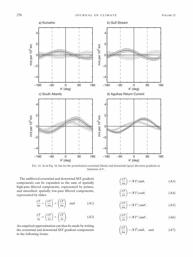
The unfiltered crosswind and downwind SST gradient

components can be expanded as the sum of spatially

high-pass filtered components, represented by primes,

and smoothed, spatially low-pass filtered components,

represented by tildes:

›T

›n5

›T

›n

� �91

f›T

›n

!and (A1)

›T

›s5

›T

›s

� �91

f›T

›s

!. (A2)

An empirical approximation can then be made by writing

the crosswind and downwind SST gradient components

in the following forms:

›T

›n

� �5 j$Tj sinu, (A3)

›T

›s

� �5 j$Tj cosu, (A4)

›T

›n

� �95 j$T9j sinu9, (A5)

›T

›s

� �95 j$T9j sinu9, (A6)

f›T

›n

!5 j$ eTj sin~u, and (A7)

FIG. 14. As in Fig. 10, but for the perturbation crosswind (black) and downwind (gray) direction gradients as

functions of u9.

276 J O U R N A L O F C L I M A T E VOLUME 23

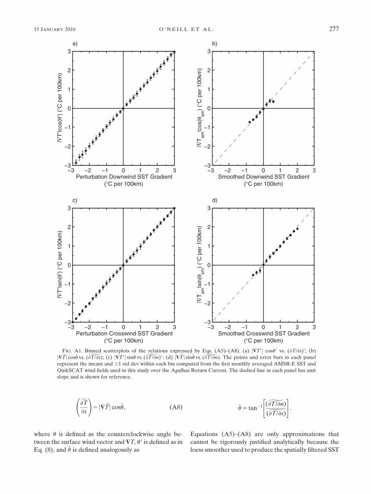
f›T

›s

!5 j$ eTj cos~u, (A8)

where u is defined as the counterclockwise angle be-

tween the surface wind vector and $T, u9 is defined as in

Eq. (8), and ~u is defined analogously as

~u 5 tan�1e(›T/›n)e(›T/›s)

" #.

Equations (A5)–(A8) are only approximations that

cannot be rigorously justified analytically because the

loess smoother used to produce the spatially filtered SST

FIG. A1. Binned scatterplots of the relations expressed by Eqs. (A5)–(A8). (a) j$T9j cosu9 vs. (›T/›s)9; (b)

j$ eTj cos~u vs.e(›T/›s); (c) j$T9j sin~u vs.e(›T/›n)9; (d) j$ eTj sin~u vs.e(›T/›n). The points and error bars in each panel

represent the means and 61 std dev within each bin computed from the first monthly averaged AMSR-E SST and

QuikSCAT wind fields used in this study over the Agulhas Return Current. The dashed line in each panel has unit

slope and is shown for reference.

15 JANUARY 2010 O ’ N E I L L E T A L . 277

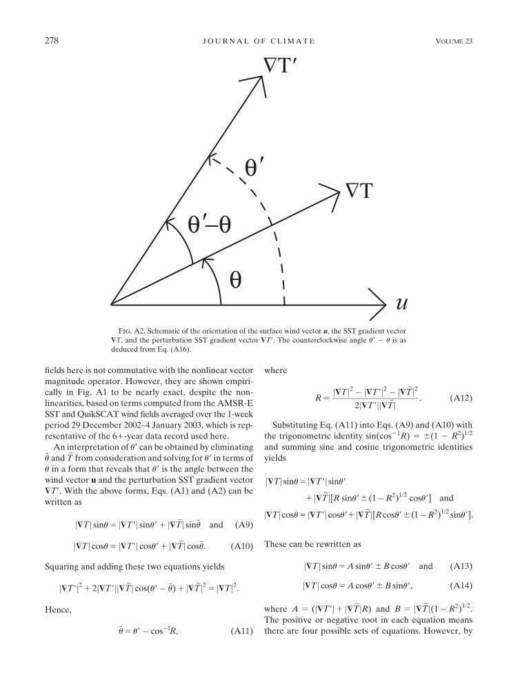
fields here is not commutative with the nonlinear vector

magnitude operator. However, they are shown empiri-

cally in Fig. A1 to be nearly exact, despite the non-

linearities, based on terms computed from the AMSR-E

SST and QuikSCAT wind fields averaged over the 1-week

period 29 December 2002–4 January 2003, which is rep-

resentative of the 61-year data record used here.

An interpretation of u9 can be obtained by eliminating~u and eT from consideration and solving for u9 in terms of

u in a form that reveals that u9 is the angle between the

wind vector u and the perturbation SST gradient vector

$T9. With the above forms, Eqs. (A1) and (A2) can be

written as

j$Tj sinu 5 j$T9j sinu9 1 j$ eTj sin~u and (A9)

j$Tj cosu 5 j$T9j cosu9 1 j$ eTj cos~u. (A10)

Squaring and adding these two equations yields

j$T9j2 1 2j$T9jj$ eTj cos(u9� ~u) 1 j$ eTj2 5 j$Tj2.

Hence,

~u 5 u9� cos�1R, (A11)

where

R 5j$Tj2 � j$T9j2 � j$ eTj2

2j$T9jj$ eTj . (A12)

Substituting Eq. (A11) into Eqs. (A9) and (A10) with

the trigonometric identity sin(cos21R) 5 6(1 2 R2)1/2

and summing sine and cosine trigonometric identities

yields

j$Tj sinu5 j$T9j sinu9

1 j$ eTj[R sinu96(1�R2)1/2 cosu9] and

j$Tjcosu5 j$T9jcosu91 j$ eTj[Rcosu96(1�R2)1/2 sinu9].

These can be rewritten as

j$Tj sinu 5 A sinu9 6 B cosu9 and (A13)

j$Tj cosu 5 A cosu9 6 B sinu9, (A14)

where A 5 (j$T9j1 j$ eTjR) and B 5 j$ eTj(1� R2)1/2.

The positive or negative root in each equation means

there are four possible sets of equations. However, by

FIG. A2. Schematic of the orientation of the surface wind vector u, the SST gradient vector

$T, and the perturbation SST gradient vector $T9. The counterclockwise angle u9 2 u is as

deduced from Eq. (A16).

278 J O U R N A L O F C L I M A T E VOLUME 23

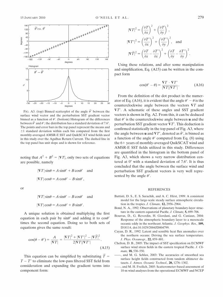
noting that A2 1 B2 5 j$Tj, only two sets of equations

are possible, namely

j$Tj sinu 5 A sinu9 1 B cosu9 and

j$Tj cosu 5 A cosu9� B sinu9,

or

j$Tj sinu 5 A sinu9� B cosu9 and

j$Tj cosu 5 A cosu9 1 B sinu9.

A unique solution is obtained multiplying the first

equation in each pair by sinu9 and adding it to cosu9

times the second equation. Doing so to both sets of

equations gives the same result:

cos(u� u9) 5A

j$Tj 5j$Tj2 1 j$T9j2 � j$ eTj2

2j$Tjj$T9j .

(A15)

This equation can be simplified by substituting eT 5

T � T9 to eliminate the low-pass filtered SST field from

consideration and expanding the gradient terms into

component form:

j$Tj2 5›T

›x

� �2

1›T

›y

� �2

,

j$T9j2 5›T9

›x

� �2

1›T9

›y

� �2

, and

j$ eTj2 5›T

›x� ›T9

›x

� �2

1›T

›y� ›T9

›y

� �2

.

Using these relations, and after some manipulation

and simplification, Eq. (A15) can be written in the com-

pact form

cos(u9� u) 5$T � $T9

j$Tjj$T9j . (A16)

From the definition of the dot product in the numer-

ator of Eq. (A16), it is evident that the angle u9 2 u is the

counterclockwise angle between the vectors $T and

$T9. A schematic of these angles and SST gradient

vectors is shown in Fig. A2. From this, it can be deduced

that u9 is the counterclockwise angle between u and the

perturbation SST gradient vector $T9. This deduction is

confirmed statistically in the top panel of Fig. A3, where

the angle between u and $T9, denoted as u9, is binned as

a function of the angle u9 computed from Eq. (8) using

the 61 years of monthly-averaged QuikSCAT wind and

AMSR-E SST fields utilized in this study. Differences

are quantified in the histogram in the bottom panel of

Fig. A3, which shows a very narrow distribution cen-

tered at 08 with a standard deviation of 7.68. It is thus

concluded that the angle between the surface wind and

perturbation SST gradient vectors is very well repre-

sented by the angle u9.

REFERENCES

Battisti, D. S., E. S. Sarachik, and A. C. Hirst, 1999: A consistent

model for the large-scale steady surface atmospheric circula-

tion in the tropics. J. Climate, 12, 2956–2964.

Bond, N. A., 1992: Observations of planetary boundary-layer struc-

ture in the eastern equatorial Pacific. J. Climate, 5, 699–706.

Bourras, D., G. Reverdin, H. Giordani, and G. Caniaux, 2004:

Response of the atmospheric boundary layer to a mesoscale

oceanic eddy in the northeast Atlantic. J. Geophys. Res., 109,

D18114, doi:10.1029/2004JD004799.

Cayan, D. R., 1992: Latent and sensible heat flux anomalies over

the northern oceans: Driving the sea surface temperature.

J. Phys. Oceanogr., 22, 859–881.

Chelton, D. B., 2005: The impact of SST specification on ECMWF

surface wind stress fields in the eastern tropical Pacific. J. Cli-

mate, 18, 530–550.

——, and M. G. Schlax, 2003: The accuracies of smoothed sea

surface height fields constructed from tandem altimeter da-

tasets. J. Atmos. Oceanic Technol., 20, 1276–1302.

——, and M. H. Freilich, 2005: Scatterometer-based assessment of

10-m wind analyses from the operational ECMWF and NCEP

FIG. A3. (top) Binned scatterplot of the angle bu9 between the

surface wind vector and the perturbation SST gradient vector

binned as a function of u9. (bottom) Histogram of the differences

between bu9 and u9; the distribution has a standard deviation of 7.68.

The points and error bars in the top panel represent the means and

61 standard deviation within each bin computed from the first

monthly-averaged AMSR-E SST and QuikSCAT wind fields used

in this study over the Agulhas Return Current. The dashed line in

the top panel has unit slope and is shown for reference.

15 JANUARY 2010 O ’ N E I L L E T A L . 279

numerical weather prediction models. Mon. Wea. Rev., 133,

409–429.

——, and F. J. Wentz, 2005: Global microwave satellite observations

of sea surface temperature for numerical weather prediction and

climate research. Bull. Amer. Meteor. Soc., 86, 1097–1115.

——, and Coauthors, 2001: Observations of coupling between

surface wind stress and sea surface temperature in the eastern

tropical Pacific. J. Climate, 14, 1479–1498.

——, M. G. Schlax, M. H. Freilich, and R. F. Milliff, 2004: Satellite

measurements reveal persistent small-scale features in ocean

winds. Science, 303, 978–983.

——, ——, and R. M. Samelson, 2007: Summertime coupling be-

tween sea surface temperature and wind stress in the Cal-

ifornia Current System. J. Phys. Oceanogr., 37, 495–517.

Cleveland, W. S., and S. J. Devlin, 1988: Locally weighted re-

gression: An approach to regression analysis by local fitting.

J. Amer. Stat. Assoc., 83, 596–610.

Cronin, M. F., S.-P. Xie, and H. Hashizume, 2003: Barometric

pressure variations associated with eastern Pacific tropical

instability waves. J. Climate, 16, 3050–3057.

de Szoeke, S. P., and C. S. Bretherton, 2004: Quasi-Lagrangian large

eddy simulations of cross-equatorial flow in the east Pacific at-

mospheric boundary layer. J. Atmos. Sci., 61, 1837–1858.

——, ——, N. A. Bond, M. F. Cronin, and B. M. Morley, 2005:

EPIC 958W observations of the eastern Pacific atmosphere

boundary layer from the cold tongue to the ITCZ. J. Atmos.

Sci., 62, 426–442.

Ebuchi, N., H. C. Graber, and M. J. Caruso, 2002: Evaluation of

wind vectors observed by QuikSCAT/SeaWinds using ocean

buoy data. J. Atmos. Oceanic Technol., 19, 2049–2062.

Freihe, C. A., and Coauthors, 1991: Air–sea fluxes and surface layer

turbulence around a sea surface temperature front. J. Geo-

phys. Res., 96, 8593–8609.

Haack, T., D. Chelton, J. Pullen, J. D. Doyle, and M. Schlax, 2008:

Summertime influence of SST on surface wind stress off the

U.S. west coast from the U.S. Navy COAMPS model. J. Phys.

Oceanogr., 38, 2414–2437.

Haltiner, G. J., and F. L. Martin, 1957: Dynamical and Physical

Meteorology. McGraw-Hill, 470 pp.

Hashizume, H., S.-P. Xie, M. Fujiwara, M. Shiotani, T. Watanabe,

Y. Tanimoto, W. T. Liu, and K. Takeuchi, 2002: Direct ob-

servations of atmospheric boundary layer response to SST

variations associated with tropical instability waves over the

eastern equatorial Pacific. J. Climate, 15, 3379–3393.

Hayes, S. P., M. J. McPhaden, and J. M. Wallace, 1989: The in-

fluence of sea-surface temperature on surface wind in the

eastern equatorial Pacific. J. Climate, 2, 1500–1506.

Hogg, A. C. M., W. K. Dewar, P. Berloff, S. Kravtsov, and

D. K. Hutchinson, 2009: The effects of mesoscale ocean–

atmosphere coupling on the large-scale ocean circulation.

J. Climate, 22, 4066–4082.

Holton, J. R., 1992: An Introduction to Dynamic Meteorology. 1st ed.

Academic Press, 511 pp.

Jin, X., C. Dong, J. Kurian, J. C. McWilliams, D. B. Chelton, and

Z. Li, 2009: SST–wind interaction in coastal upwelling: Oceanic

simulation with empirical coupling. J. Phys. Oceanogr., 39, 2957–

2970.

Jury, M. R., 1994: Thermal front within the marine atmospheric

boundary layer over the Agulhas Current south of Africa:

Composite aircraft observations. J. Geophys. Res., 99, 3297–3304.

Lindzen, R. S., and S. Nigam, 1987: On the role of sea surface

temperature gradients in forcing low-level winds and conver-

gence in the tropics. J. Atmos. Sci., 44, 2418–2436.

Liu, W. T., and W. Tang, 1996: Equivalent neutral wind. JPL

Publication 96–17, 8 pp.

——, X. Xie, and P. Niiler, 2007: Ocean–atmosphere interaction

over Agulhas Extension meanders. J. Climate, 20, 5784–5797.

Mahrt, L., D. Vickers, and E. Moore, 2004: Flow adjustments

across sea-surface temperature changes. Bound.-Layer Me-

teor., 111, 553–564.

Maloney, E. D., and D. B. Chelton, 2006: An assessment of the sea

surface temperature influence on surface wind stress in numerical

weather prediction and climate models. J. Climate, 19, 2743–2762.

Mantua, N. J., S. R. Hare, Y. Zhang, J. M. Wallace, and

R. C. Francis, 1997: A Pacific interdecadal climate oscillation

with impacts on salmon production. Bull. Amer. Meteor. Soc.,

78, 1069–1079.

Mears, C. A., D. K. Smith, and F. J. Wentz, 2001: Comparison of

Special Sensor Microwave Imager and buoy-measured wind

speeds from 1987 to 1997. J. Geophys. Res., 106, 11 719–11 729.

Mey, R. D., and N. D. Walker, 1990: Surface heat fluxes and marine

boundary layer modification in the Agulhas Retroflection re-

gion. J. Geophys. Res., 95, 15 997–16 015.

Milliff, R. F., W. G. Large, W. R. Holland, and J. C. McWilliams,

1996: The general circulation responses of high-resolution

North Atlantic Ocean models to synthetic scatterometer

winds. J. Phys. Oceanogr., 26, 1747–1768.

Nonaka, M., and S.-P. Xie, 2003: Covariations of sea surface tem-

perature and wind over the Kuroshio and its extension: Evidence

for ocean-to-atmosphere feedback. J. Climate, 16, 1404–1413.

Norris, J. R., and S. F. Iacobellis, 2005: North Pacific cloud feed-

backs inferred from synoptic-scale dynamic and thermody-

namic relationships. J. Climate, 18, 4862–4878.

Okumura, Y., S.-P. Xie, A. Numaguti, and Y. Tanimoto, 2001:

Tropical Atlantic air–sea interaction and its influence on the

NAO. Geophys. Res. Lett., 28, 1507–1510.

O’Neill, L. W., D. B. Chelton, and S. K. Esbensen, 2003: Obser-

vations of SST-induced perturbations on the wind stress field

over the Southern Ocean on seasonal time scales. J. Climate,

16, 2340–2354.

——, ——, ——, and F. J. Wentz, 2005: High-resolution satellite

measurements of the atmospheric boundary layer response to

SST perturbations over the Agulhas Return Current. J. Cli-

mate, 18, 2706–2723.

——, S. K. Esbensen, N. Thum, R. M. Samelson, and D. B. Chelton,

2010: Dynamical analysis of the boundary layer and surface wind

responses to mesoscale SST perturbations. J. Climate, in press.

Park, K.-A., and P. C. Cornillon, 2002: Stability-induced modifi-

cation of sea surface winds over Gulf Stream rings. Geophys.

Res. Lett., 29, 2211, doi:10.1029/2001GL014236.

——, ——, and D. L. Codiga, 2006: Modification of surface winds

near ocean fronts: Effects of Gulf Stream rings on scatterom-

eter (QuikSCAT, NSCAT) wind observations. J. Geophys.

Res., 111, C03021, doi:10.1029/2005JC003016.

Rouault, M., and J. R. E. Lutjeharms, 2000: Air–sea exchange over

an Agulhas eddy at the subtropical convergence. Global At-

mos. Ocean Syst., 7, 125–150.

Samelson, R. M., E. D. Skyllingstad, D. B. Chelton, S. K. Esbensen,

L. W. O’Neill, and N. Thum, 2006: On the coupling of wind

stress and sea surface temperature. J. Climate, 19, 1557–1566.

Schlax, M. G., D. B. Chelton, and M. H. Freilich, 2001: Sampling

errors in wind fields constructed from single and tandem scat-

terometer datasets. J. Atmos. Oceanic Technol., 18, 1014–1036.

Seo, H., A. J. Miller, and J. O. Roads, 2007: The Scripps coupled

ocean–atmosphere regional (SCOAR) model, with applica-

tions in the eastern Pacific sector. J. Climate, 20, 381–402.

280 J O U R N A L O F C L I M A T E VOLUME 23

Skyllingstad, E. D., D. Vickers, L. Mahrt, and R. Samelson, 2006:

Effects of mesoscale sea-surface temperature fronts on the

marine atmospheric boundary layer. Bound.-Layer Meteor.,

123, 219–237, doi:10.1007/s10546-006-9127-8.

Small, R. J., S.-P. Xie, and Y. Wang, 2003: Numerical simulation

of atmospheric response to Pacific tropical instability waves.

J. Climate, 16, 3723–3741.

——, ——, and J. Hafner, 2005a: Satellite observations of meso-

scale ocean features and copropagating atmospheric surface

fields in the tropical belt. J. Geophys. Res., 110, C02021,

doi:10.1029/2004JC002598.

——, ——, Y. Wang, S. K. Esbensen, and D. Vickers, 2005b:

Numerical simulation of boundary layer structure and cross-

equatorial flow in the eastern Pacific. J. Atmos. Sci., 62, 1812–

1830.

——, and Coauthors, 2008: Air–sea interaction over ocean fronts

and eddies. Dyn. Atmos. Oceans, 45, 274–319, doi:10.1016/

j.dynatmoce.2008.01.001.

——, K. J. Richards, S.-P. Xie, P. Dutrieux, and T. Miyama, 2009:

Damping of tropical instability waves caused by the action

of surface currents on stress. J. Geophys. Res., 114, C04009,

doi:10.1029/2008JC005147.

Song, Q., T. Hara, P. Cornillon, and C. A. Friehe, 2004: A com-

parison between observations and MM5 simulations of the

marine atmospheric boundary layer across a temperature front.

J. Atmos. Oceanic Technol., 21, 170–178.

——, P. Cornillon, and T. Hara, 2006: Surface wind response to

oceanic fronts. J. Geophys. Res., 111, C12006, doi:10.1029/

2006JC003680.

——, D. B. Chelton, S. K. Esbensen, N. Thum, and L. W. O’Neill,

2009: Coupling between sea surface temperature and low-level

winds in mesoscale numerical models. J. Climate, 22, 146–164.

Spall, M. A., 2007a: Effect of sea surface temperature–wind stress

coupling on baroclinic instability in the ocean. J. Phys. Ocean-

ogr., 37, 1092–1097.

——, 2007b: Midlatitude wind stress–sea surface temperature cou-

pling in the vicinity of oceanic fronts. J. Climate, 20, 3785–

3801.

Stevens, B., J. Duan, J. C. McWilliams, M. Munnich, and J. D. Neelin,

2002: Entrainment, Rayleigh friction, and boundary layer winds

over the tropical Pacific. J. Climate, 15, 30–44.

Sweet, W. R., R. Fett, J. Kerling, and P. LaViolette, 1981: Air–sea

interaction effects in the lower troposphere across the north

wall of the Gulf Stream. Mon. Wea. Rev., 109, 1042–1052.

Thum, N., 2006: Atmospheric boundary layer coupling to mid-

latitude mesoscale sea surface temperature anomalies. Ph.D.

thesis, Oregon State University, 142 pp. [Available from Uni-

versity Microfilm, 305 N. Zeeb Rd., Ann Arbor, MI 48106.]

Tokinaga, H., and Coauthors, 2006: Atmospheric sounding over

the winter Kuroshio Extension: Effect of surface stability on

atmospheric boundary layer structure. Geophys. Res. Lett., 33,

L04703, doi:10.1029/2005GL025102.

Wai, M., and S. A. Stage, 1989: Dynamical analysis of marine at-

mospheric boundary layer structure near the Gulf Stream

oceanic front. Quart. J. Roy. Meteor. Soc., 115, 29–44.

Wallace, J. M., T. P. Mitchell, and C. Deser, 1989: The influence of

sea surface temperature on surface wind in the eastern equa-

torial Pacific: Seasonal and interannual variability. J. Climate,

2, 1492–1499.

Warner, T. T., M. N. Lakhtakia, J. D. Doyle, and R. A. Pearson,

1990: Marine atmospheric boundary layer circulations forced

by Gulf Stream sea surface temperature gradients. Mon. Wea.

Rev., 118, 309–323.

Wentz, F. J., and T. Meissner, 2000: AMSR Ocean Algorithm, ver-

sion 2. Tech. Rep. 121599A–1, Remote Sensing Systems, 66 pp.

White, W. B., and J. L. Annis, 2003: Coupling of extratropical

mesoscale eddies in the ocean to westerly winds in the atmo-

spheric boundary layer. J. Climate, 33, 1095–1107.

Xie, S.-P., 2004: Satellite observations of cool ocean–atmosphere

interaction. Bull. Amer. Meteor. Soc., 85, 195–208.

15 JANUARY 2010 O ’ N E I L L E T A L . 281

Copyright of Journal of Climate is the property of American Meteorological Society and its content may not be

copied or emailed to multiple sites or posted to a listserv without the copyright holder's express written

permission. However, users may print, download, or email articles for individual use.