Moisture transport in midlatitude cyclones - CentAURcentaur.reading.ac.uk/19144/3/783_ftp.pdf · Moisture transport in midlatitude cyclones ... Moisturetransportinmidlatitudecyclones

Moisture transport in midlatitude cyclones Article

Published Version

Boutle, I. A., Belcher, S. E. and Plant, R. S. (2011) Moisture transport in midlatitude cyclones. Quarterly Journal of the Royal Meteorological Society, 137 (655). pp. 360373. ISSN 1477870X doi: https://doi.org/10.1002/qj.783 Available at http://centaur.reading.ac.uk/19144/

It is advisable to refer to the publisher’s version if you intend to cite from the work.

To link to this article DOI: http://dx.doi.org/10.1002/qj.783

Publisher: Royal Meteorological Society

All outputs in CentAUR are protected by Intellectual Property Rights law, including copyright law. Copyright and IPR is retained by the creators or other copyright holders. Terms and conditions for use of this material are defined in the End User Agreement .

www.reading.ac.uk/centaur

CentAUR

Central Archive at the University of Reading

Reading’s research outputs online

http://centaur.reading.ac.uk/licence

http://www.reading.ac.uk/centaur

Quarterly Journal of the Royal Meteorological Society Q. J. R. Meteorol. Soc. 137: 360–373, January 2011 B

Moisture transport in midlatitude cyclones

I. A. Boutle,* S. E. Belcher and R. S. PlantDepartment of Meteorology, University of Reading, Reading, UK

*Correspondence to: I. A. Boutle, Met Office, FitzRoy Road, Exeter, EX1 3PB, UK.E-mail: [email protected]

We discuss how synoptic-scale variability controls the transport of atmosphericwater vapour by midlatitude cyclones. Idealized simulations are used to investigatequantitatively which factors determine the magnitude of cyclone moisture transport.It is demonstrated that large-scale ascent on the warm conveyor belt and shallowcumulus convection are equally important for ventilating moisture from theboundary layer into the free troposphere, and that ventilated moisture can betransported large distances eastwards and polewards by the cyclone, before beingreturned to the surface as precipitation.

The initial relative humidity is shown to have little effect on the ability of thecyclone to transport moisture, whilst the absolute temperature and meridionaltemperature gradient provide much stronger controls. Scaling arguments arepresented to quantify the dependence of moisture transport on large-scale andboundary-layer parameters. It is shown that ventilation by shallow convectionand warm-conveyor-belt advection vary in the same way with changes to large-scale parameters. However, shallow convective ventilation has a much strongerdependence on boundary-layer parameters than warm-conveyor-belt ventilation.Copyright c© 2011 Royal Meteorological Society

Key Words: warm conveyor belts; convection; boundary-layer ventilation; water cycle

Received 21 July 2010; Revised 9 December 2010; Accepted 4 January 2011; Published online in Wiley OnlineLibrary

Citation: Boutle IA, Belcher SE, Plant RS. 2011. Moisture transport in midlatitude cyclones. Q. J. R. Meteorol.Soc. 137: 360–373. DOI:10.1002/qj.783

1. Introduction

The pattern of water vapour in the troposphere is shapedby processes on a wide variety of scales, from evaporation atthe surface, through boundary-layer mixing and convection,synoptic- and global-scale motions, to precipitation back tothe surface. Schneider et al. (2006) developed a climatologyof the zonal-mean structure of tropospheric water vapourand the zonal-mean fluxes that shape this pattern. In generalterms, the sources of water vapour are at the surface in thetropics and subtropics. Synoptic-scale eddies then flux thiswater vapour into the upper troposphere in the extratropics.Furthermore, Trenberth and Stepaniak (2003) demonstratethat this latent energy transport accounts for approximatelyhalf of the atmospheric energy flux in the midlatitudes. Astriking conclusion of these studies is that the poleward

moisture flux, carried mainly by synoptic-scale eddies, notonly determines the precipitation distribution but also playsa significant role in shaping the temperature structure of theplanet. This raises the question of how transport is achievedon the scale of an individual weather system.

A recent article by Boutle et al. (2010) has investigated theboundary-layer structure and low-level moisture transportin an idealized, numerically simulated baroclinic wave.Boundary-layer budgeting techniques were used to quantifyevaporation, transport within and ventilation of moisturefrom the boundary layer. It was shown that large-scaleventilation on the warm conveyor belt (WCB) was of similarimportance to shallow convective ventilation in cumulusclouds, demonstrating that both processes play an importantrole in the vertical transport of moisture from the surfaceinto the free troposphere. However, they did not investigate

Copyright c© 2011 Royal Meteorological Society

Cyclone Moisture Transport 361

how moisture was transported zonally or meridionallywithin the free troposphere. WCBs are often consideredto be the primary mechanism for tropospheric transportby cyclones (Wernli, 1997; Eckhardt et al., 2004), but whatfactors control the moisture transport by WCBs? Similarly, ifconvective processes are important for ventilating moisturefrom the boundary layer, what happens to the moistureonce it is ventilated and what factors control this moisturetransport?

Quantifying cyclone moisture transport can help us tounderstand the role larger-scale processes play in shapingthe global water cycle. For example, the North AtlanticOscillation (NAO) is known to exert a strong controlover the midlatitude jet, causing variations in its strengthand orientation which, in turn, exert a control over thestrength and location of midlatitude cyclones. Stohl et al.(2008) demonstrated that in a positive phase of the NAO,characterized by a stronger midlatitude jet, subtropicalsources of moisture are important for heavy rainfall eventsin mid to high latitudes. Ruprecht et al. (2002) alsodemonstrated higher polewards moisture transport in apositive phase of the NAO, linked to more intense cyclonesproducing the transport. They also showed that the locationof maximum moisture transport was shifted further northin a positive NAO, linked to a poleward shift of the jetunder positive NAO conditions. Whilst these studies providequalitative evidence for the link between jet strength andmoisture transport, they do not quantify how moisturetransport can be expected to change with a given change injet strength.

There are also important climatological questions that canbe answered by investigating cyclone moisture transport.Recent articles by Field and Wood (2007) and Fieldet al. (2008) have discussed the structure of cyclones ina composite of both real-world events and climate-modelsimulations. They discussed how the cyclone-averaged near-surface wind speed 〈V〉 and water-vapour path 〈WVP〉could be used as independent metrics of cyclone intensityand moisture availability to explain a considerable amountof observed variability. They showed how the WCB rainrate was proportional to the product of these two metrics,and that 〈WVP〉 increased with increasing sea-surfacetemperature (SST) according to the Clausius–Clapeyronequation. They also discussed the implications of their resultson the way cyclones may change in a warming climate. Allenand Ingram (2002) discuss how the Clausius–Clapeyronequation should give a 6.5% K−1 increase in globalatmospheric water-vapour storage, but the total globalprecipitation should only increase at 2% K−1, constrained bythe global energy balance. Hence Field and Wood (2007) andField et al. (2008) suggested that cyclones should be fewer innumber or less intense to account for this difference, effectsthat have both been seen in modelling studies (Meehl et al.,2007; Bengtsson et al., 2006), but it is presently unclear whichprocess is more likely. Could the necessary adjustment beachieved through changes in the jet?

This article aims to address the questions raised above,focusing on an individual baroclinic system to determinethe controls on the cycling of water vapour throughthe system. We aim to quantify the dominant controlson moisture transport from large-scale and convectivemotions, and to establish a scaling for these processes.Section 2 introduces the idealized model used, with section 3describing the moisture cycle in the control simulation.

In section 4 we investigate how changes to large-scaleparameters influence the moisture cycle. In section 4.1,changes to the initial relative humidity distribution areinvestigated, demonstrating why the idea that relativehumidity remains approximately constant (Allen andIngram, 2002; Field and Wood, 2007) works for baroclinicwaves. Section 4.2 investigates the effect of the absoluteatmospheric temperature on the cyclone moisture cycle,with section 4.3 considering the effect of the meridionaltemperature gradient. Scaling arguments for how theselarge-scale changes affect both advective and convectivemoisture ventilation from the boundary layer are givenin section 5. Section 6 then discusses how changes to theboundary-layer structure can have markedly different effectson the two ventilation processes, before conclusions aredrawn in section 7.

2. Model description

The control simulation used in this article is the sameas that used in Boutle et al. (2010), who presented anidealized baroclinic-wave simulation similar to that denotedLC1 by Thorncroft et al. (1993). The Met Office UnifiedModel (MetUM) is used in idealized mode, allowingus to use its full range of physical parametrizations tomodel turbulent and moist atmospheric processes. TheMetUM employs a semi-Lagrangian advection scheme,with semi-implicit time integration. For this study, thedynamics are coupled to physical parametrizations ofboundary-layer turbulence, shallow and deep convection,mixed-phase microphysics and large-scale cloud. Thesedynamics and physics schemes are similar to those usedin the operational global forecast model and the HadGEM1climate model, and full details of the schemes can be foundin Martin et al. (2006) and references therein. The modelis configured on a limited-area domain of 60◦ longitudeby 80◦ latitude, at 0.4◦ horizontal resolution and with38 staggered vertical levels below 40 km, giving the finestresolution near the surface. East–west periodic boundaryconditions are applied, giving wavenumber-6 symmetry toour simulations.

The large meridional extent is chosen in order that thenorth–south boundaries do not affect the simulations. Themodel is also configured on a Cartesian f -plane. This choiceis made as we wish to vary the Coriolis parameter todetermine its influence on moisture transport, and the useof a Cartesian f -plane ensures that the size of cyclone doesnot change and therefore the area over which ventilationoccurs is unaffected. The differences between cyclones inspherical and Cartesian geometry are well documented inthe literature (Balasubramanian and Garner, 1997; Wernliet al., 1998), with the main difference being that Cartesiansimulations tend to be more cyclonic in nature. Theaddition of a barotropic cyclonic shear to a sphericalsimulation leads to a simulation very similar to our Cartesianone. Furthermore, Wernli et al. (1998) describe how thisCartesian simulation is similar to the conceptual model ofShapiro and Keyser (1990), with a T-bone frontal structuredeveloping and a bent-back warm front wrapping aroundthe low centre.

Copyright c© 2011 Royal Meteorological Society Q. J. R. Meteorol. Soc. 137: 360–373 (2011)

362 I. A. Boutle et al.

The initialization follows that of Polvani and Esler (2007)to specify the initial-condition wind field analytically as

u(φ, z) = U0 sin3[π sin2(φ)]z

zTexp

(− (z/zT)2 − 1

2

),

(1)

where φ is the latitude, z is the height, U0 = 45 m s−1 is themaximum jet speed and zT = 13 km is the temperature scaleheight. A temperature profile in thermal wind balance withthis is then constructed, integrated from a vertical profileof constant static stability (4 K km−1 below zT , 16 K km−1

above) and surface temperature of T0 = 280 K at 45◦N (thejet centre). A pressure profile is constructed in hydrostaticbalance, and the model is run for several time steps to allowthe wind, temperature and pressure fields to adjust to thenonlinear balance consistent with the equation set of theMetUM. The moisture field is initialized in terms of relativehumidity (RH) as

RH(φ, z) ={

RH0[1 − 0.9R(φ)(z/zq)5/4] z < zq,RH0(0.0625) z > zq,

(2)

where RH0 = 80%, zq = 12 km and R(φ) defines thelatitudinal variation of RH as given in Boutle et al.(2010). The sea-surface temperature is fixed throughout thesimulation and equal to the initial temperature of the lowestmodel level. The jet structure is baroclinically unstable, andso a small perturbation, given in Polvani and Esler (2007),is added to the temperature field to trigger cyclogenesis.

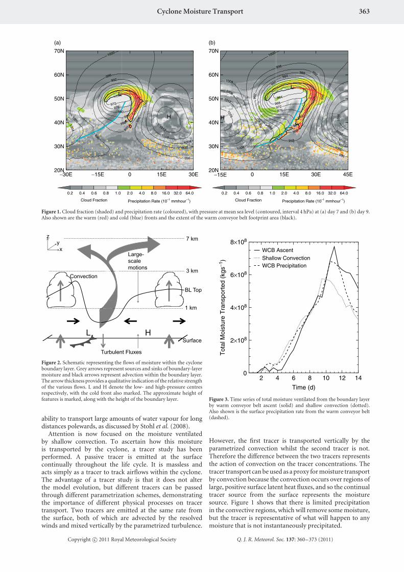
The simulations are run for 14 days, over which timean alternating series of high- and low-pressure systemsforms and intensifies. The system undergoes periods oflinear and nonlinear growth, reaching its peak intensitybetween days 10 and 11 before starting to decay. The spatialstructure of the surface pressure, fronts, cloud fraction andprecipitation rate at days 7 and 9 is shown in Figure 1. Itshows many features of a typical midlatitude weather system,such as the main precipitation band located in the WCB.This poleward airstream of warm, moist air runs ahead of thecold front and ascends over the warm front. It splits into twobranches; one turns cyclonically and wraps around the northof the low centre, whilst the other turns anticyclonically easttowards the neighbouring high pressure. Also noticeable inFigure 1 is some cloud-free air south of the low centre,immediately behind the cold front. This is associated withthe descending air in the dry intrusion. Further behind thecold front and to the west of the cyclone centre are low-levelcumulus clouds. These are formed in a cold-air outbreak, asshallow convection is triggered by cold air flowing from thenorth over a warmer sea surface.

3. Moisture cycle of a baroclinic wave

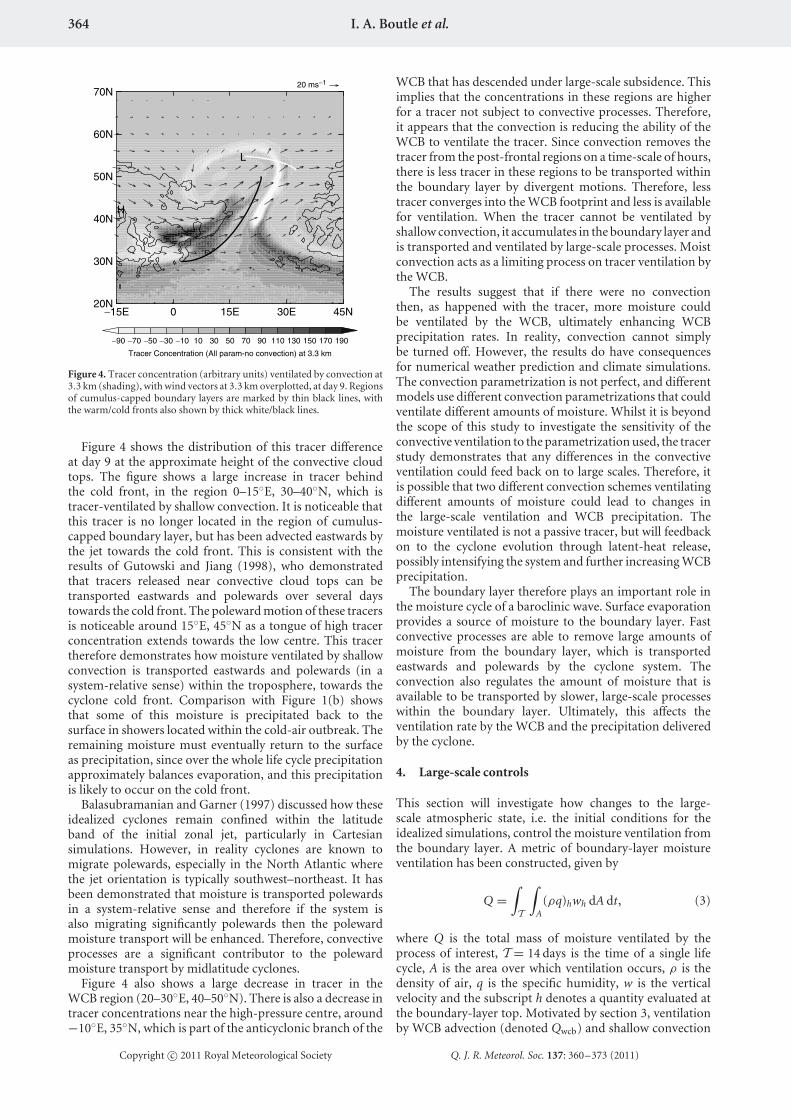
Boutle et al. (2010) discussed how moisture, evaporated fromthe sea surface, was transported through the atmosphericboundary layer and ventilated into the troposphere in twomain regions. Their results are summarized schematically inFigure 2. Moisture is evaporated from the sea surface behindthe cold front and in the high-pressure part of the wave.Approximately half of this moisture is locally ventilatedfrom the boundary layer in shallow convection in cumulusclouds above the region of positive surface fluxes. The restof the moisture is transported within the boundary layer

by divergent and convergent motions, forced by surfacedrag and large-scale ageostrophic motions. The moistureconverges into the footprint of the WCB. Here the surfacefluxes are negative and a small amount of moisture isreturned to the surface. However, most of the moisture isventilated from the boundary layer by large-scale ascent onthe WCB. Therefore, the cyclone boundary layer is capable oftaking moisture from a single source region and processingit through two separate ventilation regions.

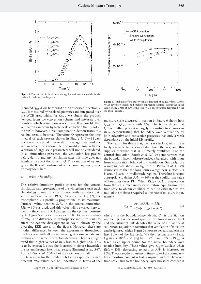
Figure 3 shows a time series of boundary-layer ventilationfrom these two processes over the life cycle. The WCBventilation is calculated as the moisture flux through theboundary-layer top in the WCB area. Here, the WCBarea is defined using the method of Sinclair et al. (2008),which locates the 95th percentile of the entire verticalvelocity on boundary-layer top dataset and defines theWCB as any ascent greater than this value. Sinclair et al.(2008) demonstrated that this definition finds the majorityof the WCB, rather than just the core. Increasing thepercentile would result in only part of the WCB ventilationbeing observed, whereas reducing the percentile leads tothe inclusion of areas that are not part of the WCB.The convective ventilation is calculated directly from themoisture flux parametrized by the convection scheme,summed over all points on which the convection schemeis active. Both processes start ventilating around day 4,with shallow convection ventilating at a slightly fasterrate than the WCB up to day 8. The shallow convectiveventilation peaks at day 10 before decaying, whilst the WCBventilation continues to day 11, coincident with the peakeddy kinetic energy (EKE) of the simulation. The WCBventilation also peaks approximately 20% higher than theconvective ventilation before starting to decay at a similarrate. This increased peak means that, over the life cycle,the WCB ventilates ≈ 10% more moisture than the shallowconvection.

Figure 3 also shows the precipitation rate from the WCB.Here, we define the WCB precipitation as that produced bythe large-scale ascent of the WCB, ensuring that we trackthe large-scale moisture flow responsible for boundary-layer ventilation by the WCB. There is some additionalconvective precipitation not included in this measure,although this is mainly confined to the cold front. As shown,the precipitation rate closely matches the WCB ventilationrate, demonstrating that WCBs are approximately 100%efficient at converting moisture into precipitation. Thisfact is also demonstrated by Eckhardt et al. (2004) for aclimatology study of many WCBs. There is no time lag inthis process, due to the presence of a background moistureprofile. As soon as ascent starts (around day 3), somemoisture present within the troposphere is forced to ascendpast its lifting condensation level, condensing into cloudand precipitating. At the same time, moisture is ventilatedfrom the boundary layer to replace the moisture lost fromthe troposphere. Hence the conveyor-belt analogy is a goodone, as moisture is ‘loaded’ on to the conveyor belt at oneend (in the boundary layer) whilst microphysical processesremove moisture at the other end (in the troposphere) atapproximately the same rate. The total moisture contentof the troposphere is largely unchanged by this process,although its spatial distribution is. Since the WCB also flowspolewards, atmospheric water vapour is moved polewardsby the WCB. Hence the WCB forms part of the cyclone’s



−30E −15E 0 15E 30E20N

30N

40N

50N

60N

70N

972976

980

984

98899

2

992

996

996

996

996

100010

00

1000

1000

1004

1004

1004

1008

1012

L

H

(a)

0.2 0.4 0.6 0.8 1.0 2.0 4.0 8.0 16.0 32.0 64.0

Cloud Fraction Precipitation Rate (10−1 mmhour−1)

−15E 0 15E 30E 45E20N

30N

40N

50N

60N

70N

964

968972976

980

980

984

984

988

988

992

992

992

996

996

996

996

1000

1000

1000

10001004

1004

1004

1008

1008

1012

1012

1016

1016

L

H

(b)

0.2 0.4 0.6 0.8 1.0 2.0 4.0 8.0 16.0 32.0 64.0

Cloud Fraction Precipitation Rate (10−1 mmhour−1)

Figure 1. Cloud fraction (shaded) and precipitation rate (coloured), with pressure at mean sea level (contoured, interval 4 hPa) at (a) day 7 and (b) day 9.Also shown are the warm (red) and cold (blue) fronts and the extent of the warm conveyor belt footprint area (black).

y

Figure 2. Schematic representing the flows of moisture within the cycloneboundary layer. Grey arrows represent sources and sinks of boundary-layermoisture and black arrows represent advection within the boundary layer.The arrow thickness provides a qualitative indication of the relative strengthof the various flows. L and H denote the low- and high-pressure centresrespectively, with the cold front also marked. The approximate height offeatures is marked, along with the height of the boundary layer.

ability to transport large amounts of water vapour for longdistances polewards, as discussed by Stohl et al. (2008).

Attention is now focused on the moisture ventilatedby shallow convection. To ascertain how this moistureis transported by the cyclone, a tracer study has beenperformed. A passive tracer is emitted at the surfacecontinually throughout the life cycle. It is massless andacts simply as a tracer to track airflows within the cyclone.The advantage of a tracer study is that it does not alterthe model evolution, but different tracers can be passedthrough different parametrization schemes, demonstratingthe importance of different physical processes on tracertransport. Two tracers are emitted at the same rate fromthe surface, both of which are advected by the resolvedwinds and mixed vertically by the parametrized turbulence.

2 4 6 8 10 12 14

Time (d)

0

2×108

4×108

6×108

8×108

Tot

al M

oist

ure

Tra

nspo

rted

(kg

s−1)

WCB AscentShallow ConvectionWCB Precipitation

Figure 3. Time series of total moisture ventilated from the boundary layerby warm conveyor belt ascent (solid) and shallow convection (dotted).Also shown is the surface precipitation rate from the warm conveyor belt(dashed).

However, the first tracer is transported vertically by theparametrized convection whilst the second tracer is not.Therefore the difference between the two tracers representsthe action of convection on the tracer concentrations. Thetracer transport can be used as a proxy for moisture transportby convection because the convection occurs over regions oflarge, positive surface latent heat fluxes, and so the continualtracer source from the surface represents the moisturesource. Figure 1 shows that there is limited precipitationin the convective regions, which will remove some moisture,but the tracer is representative of what will happen to anymoisture that is not instantaneously precipitated.



−15E 0 15E 30E 45N20N

30N

40N

50N

60N

70N20 ms−1

L

H

−90 −70 −50 −30 −10 10 30 50 70 90 110 130 150 170 190

Tracer Concentration (All param-no convection) at 3.3 km

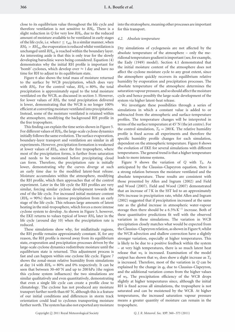
Figure 4. Tracer concentration (arbitrary units) ventilated by convection at3.3 km (shading), with wind vectors at 3.3 km overplotted, at day 9. Regionsof cumulus-capped boundary layers are marked by thin black lines, withthe warm/cold fronts also shown by thick white/black lines.

Figure 4 shows the distribution of this tracer differenceat day 9 at the approximate height of the convective cloudtops. The figure shows a large increase in tracer behindthe cold front, in the region 0–15◦E, 30–40◦N, which istracer-ventilated by shallow convection. It is noticeable thatthis tracer is no longer located in the region of cumulus-capped boundary layer, but has been advected eastwards bythe jet towards the cold front. This is consistent with theresults of Gutowski and Jiang (1998), who demonstratedthat tracers released near convective cloud tops can betransported eastwards and polewards over several daystowards the cold front. The poleward motion of these tracersis noticeable around 15◦E, 45◦N as a tongue of high tracerconcentration extends towards the low centre. This tracertherefore demonstrates how moisture ventilated by shallowconvection is transported eastwards and polewards (in asystem-relative sense) within the troposphere, towards thecyclone cold front. Comparison with Figure 1(b) showsthat some of this moisture is precipitated back to thesurface in showers located within the cold-air outbreak. Theremaining moisture must eventually return to the surfaceas precipitation, since over the whole life cycle precipitationapproximately balances evaporation, and this precipitationis likely to occur on the cold front.

Balasubramanian and Garner (1997) discussed how theseidealized cyclones remain confined within the latitudeband of the initial zonal jet, particularly in Cartesiansimulations. However, in reality cyclones are known tomigrate polewards, especially in the North Atlantic wherethe jet orientation is typically southwest–northeast. It hasbeen demonstrated that moisture is transported polewardsin a system-relative sense and therefore if the system isalso migrating significantly polewards then the polewardmoisture transport will be enhanced. Therefore, convectiveprocesses are a significant contributor to the polewardmoisture transport by midlatitude cyclones.

Figure 4 also shows a large decrease in tracer in theWCB region (20–30◦E, 40–50◦N). There is also a decrease intracer concentrations near the high-pressure centre, around−10◦E, 35◦N, which is part of the anticyclonic branch of the

WCB that has descended under large-scale subsidence. Thisimplies that the concentrations in these regions are higherfor a tracer not subject to convective processes. Therefore,it appears that the convection is reducing the ability of theWCB to ventilate the tracer. Since convection removes thetracer from the post-frontal regions on a time-scale of hours,there is less tracer in these regions to be transported withinthe boundary layer by divergent motions. Therefore, lesstracer converges into the WCB footprint and less is availablefor ventilation. When the tracer cannot be ventilated byshallow convection, it accumulates in the boundary layer andis transported and ventilated by large-scale processes. Moistconvection acts as a limiting process on tracer ventilation bythe WCB.

The results suggest that if there were no convectionthen, as happened with the tracer, more moisture couldbe ventilated by the WCB, ultimately enhancing WCBprecipitation rates. In reality, convection cannot simplybe turned off. However, the results do have consequencesfor numerical weather prediction and climate simulations.The convection parametrization is not perfect, and differentmodels use different convection parametrizations that couldventilate different amounts of moisture. Whilst it is beyondthe scope of this study to investigate the sensitivity of theconvective ventilation to the parametrization used, the tracerstudy demonstrates that any differences in the convectiveventilation could feed back on to large scales. Therefore, itis possible that two different convection schemes ventilatingdifferent amounts of moisture could lead to changes inthe large-scale ventilation and WCB precipitation. Themoisture ventilated is not a passive tracer, but will feedbackon to the cyclone evolution through latent-heat release,possibly intensifying the system and further increasing WCBprecipitation.

The boundary layer therefore plays an important role inthe moisture cycle of a baroclinic wave. Surface evaporationprovides a source of moisture to the boundary layer. Fastconvective processes are able to remove large amounts ofmoisture from the boundary layer, which is transportedeastwards and polewards by the cyclone system. Theconvection also regulates the amount of moisture that isavailable to be transported by slower, large-scale processeswithin the boundary layer. Ultimately, this affects theventilation rate by the WCB and the precipitation deliveredby the cyclone.

4. Large-scale controls

This section will investigate how changes to the large-scale atmospheric state, i.e. the initial conditions for theidealized simulations, control the moisture ventilation fromthe boundary layer. A metric of boundary-layer moistureventilation has been constructed, given by

Q =∫T

∫A

(ρq)hwh dA dt, (3)

where Q is the total mass of moisture ventilated by theprocess of interest, T = 14 days is the time of a single lifecycle, A is the area over which ventilation occurs, ρ is thedensity of air, q is the specific humidity, w is the verticalvelocity and the subscript h denotes a quantity evaluated atthe boundary-layer top. Motivated by section 3, ventilationby WCB advection (denoted Qwcb) and shallow convection



0 2 4 6 8 10 12 14

Time (d)

0

1

2

3

4

5

6

EK

E (

105 J

m−2

)

RH0=80%

RH0=90%

RH0=40%

RH0=60%

RH0=70%

Figure 5. Time series of eddy kinetic energy for various values of the initialsurface RH (shown on the plot).

(denoted Qconv) will be focused on. As discussed in section 3,Qwcb is measured by resolved quantities and integrated overthe WCB area, whilst for Qconv we obtain the product(ρq)hwh from the convection scheme and integrate overpoints at which convection is occurring. It is possible thatventilation can occur by large-scale advection that is not inthe WCB: however, direct computation demonstrates thisresidual term to be small. Therefore, Q represents the timeintegral of each process shown in Figure 3. T = 14 daysis chosen as a fixed time-scale to average over, and theway in which the cyclone lifetime might change with thevariation of large-scale parameters will not be considered.In all simulations presented, the ventilation has peakedbefore day 14 and any ventilation after this time does notsignificantly affect the value of Q. The variation of wh andqh, i.e. the flux of moisture out of the boundary layer, is theprimary focus here.

4.1. Relative humidity

The relative humidity profile chosen for the controlsimulation was representative of the wintertime storm trackclimatology, based on a comparison with reanalysis datashown in Pavan et al. (1999). As shown in Eq. (2), thetropospheric RH profile is proportional to its maximum(surface) value, denoted RH0. In the control simulationRH0 = 80% is used, and this value will be varied here toidentify the effects of RH changes on the cyclone moisturecycle. Figure 5 shows a time series of EKE for various valuesof RH0. The difference in atmospheric moisture starts toaffect the cyclone development at day 4, shown by thediverging EKE curves in the figure. However, there aremodest differences between the experiments throughoutthe life cycle, with all curves growing at a similar rate andpeaking at the same time before decaying. There is a slighttrend that higher values of RH0 lead to higher EKE. Thisis to be expected, since the increased moisture intensifiesthe system through latent-heat release (Emanuel et al., 1987;Ahmadi-Givi et al., 2004), but the variation is small.

The reasons for the similarity between experiments withdifferent RH0 values can be understood in terms of the

20 40 60 80 100

RH0 (%)

0

2×1014

4×1014

6×1014

Tot

al M

oist

ure

Tra

nspo

rted

(kg

)

WCB Advection

Shallow Convection

WCB Precipitation

Figure 6. Total mass of moisture ventilated from the boundary layer (Q) byWCB advection (solid) and shallow convection (dotted) versus the initialvalue of RH0. Also shown is the total WCB precipitation delivered by thelife cycle (dashed).

moisture cycle discussed in section 3. Figure 6 shows howQwcb and Qconv vary with RH0. The figure shows thatQ from either process is largely insensitive to changes inRH0, demonstrating that boundary-layer ventilation, byboth advective and convective processes, has only a weakdependence on the initial RH profile.

The reason for this is that, over a sea surface, moisture isfreely available to be evaporated from the sea, and thissupplies moisture that is ultimately ventilated. For thecontrol simulation, Boutle et al. (2010) demonstrated thatthe boundary-layer moisture budget is balanced, with inputfrom evaporation balanced by ventilation. Similarly, thereanalysis data shown in figure 2 of Pavan et al. (1999)demonstrates that the long-term average near-surface RHis around 80% in midlatitude regions. Therefore it seemsappropriate to define RHeq = 80% as the equilibrium valueof boundary-layer RH. When RH0 < RHeq, evaporationfrom the sea surface increases to restore equilibrium. Thetime-scale to obtain equilibrium can be estimated as theratio of the moisture required to the rate of moisture input,namely

τadj = ρqsath(RHeq − RH0)

ρCH|v1|qsat(1 − RH), (4)

where h is the boundary-layer depth, CH is the Stantonnumber, |v1| is the wind speed at the lowest model leveland the subscript ‘sat’ denotes the value of a quantity atsaturation. Equation (4) assumes that ventilation of moisturecan be ignored, which Figure 3 shows to be reasonable in thefirst 4 days of the life cycle. We then estimate h ≈ 1 km,CH ≈ 2 × 10−3 and |v1| ≈ 5 m s−1, and RH = RHeq istaken as an upper bound for the actual boundary-layerrelative humidity. These values give τadj = 2.3 days whenRH0 = 40%, decreasing to zero as RH0 is increased to80%. Therefore, the adjustment time-scale of the boundary-layer moisture content is fast compared with the life-cycletime-scale, and so the boundary-layer moisture content is



close to its equilibrium value throughout the life cycle andtherefore ventilation is not sensitive to RH0. There is aslight reduction in Q for very low RH0, due to the reducedamount of moisture available to be ventilated in early stagesof the life cycle, i.e. when t ≤ τadj. In a similar manner, whenRH0 > RHeq, the evaporation is reduced whilst ventilation isunchanged until RHeq is reached within the boundary layer.An interesting aside is that this is only true for the slowlydeveloping baroclinic waves being considered. Equation (4)demonstrates why the initial RH profile is important for‘bomb’ cyclones, which develop over ≈ 1 day and have notime for RH to adjust to its equilibrium state.

Figure 6 also shows the total mass of moisture returnedto the surface by WCB precipitation, which does varywith RH0. For the control value, RH0 = 80%, the totalprecipitation is approximately equal to the total moistureventilated on the WCB, as discussed in section 3. However,for lower values of RH0 the total precipitation deliveredis lower, demonstrating that the WCB is no longer 100%efficient at converting moisture ventilated into precipitation.Instead, some of the moisture ventilated is retained withinthe atmosphere, modifying the background RH profile inthe free troposphere.

This finding can explain the time series shown in Figure 5.For different values of RH0, the large-scale cyclone dynamicsinitially follows the same evolution. The surface evaporation,boundary-layer transport and ventilation are similar in allexperiments. However, precipitation formation is weakenedat lower values of RH0, since the free troposphere, wheremost of the precipitation forms, is further from saturationand needs to be moistened before precipitating cloudcan form. Therefore, the precipitation rate is initiallylower, demonstrating why the curves diverge at suchan early time due to the modified latent-heat release.Moisture accumulates within the atmosphere, modifyingthe RH profile, which then approaches that of the controlexperiment. Later in the life cycle the RH profiles are verysimilar, forcing similar cyclone development towards theend of the life cycle. For increased initial moisture content(RH0 = 90%) there is intense precipitation from an earlystage of the life cycle. This releases large amounts of latentheating in the mid-troposphere, which forces a more intensecyclone system to develop. As shown in Figure 5, however,the EKE returns to values typical of lower RH0 later in thelife cycle (around day 10) when the precipitation rate isreduced.

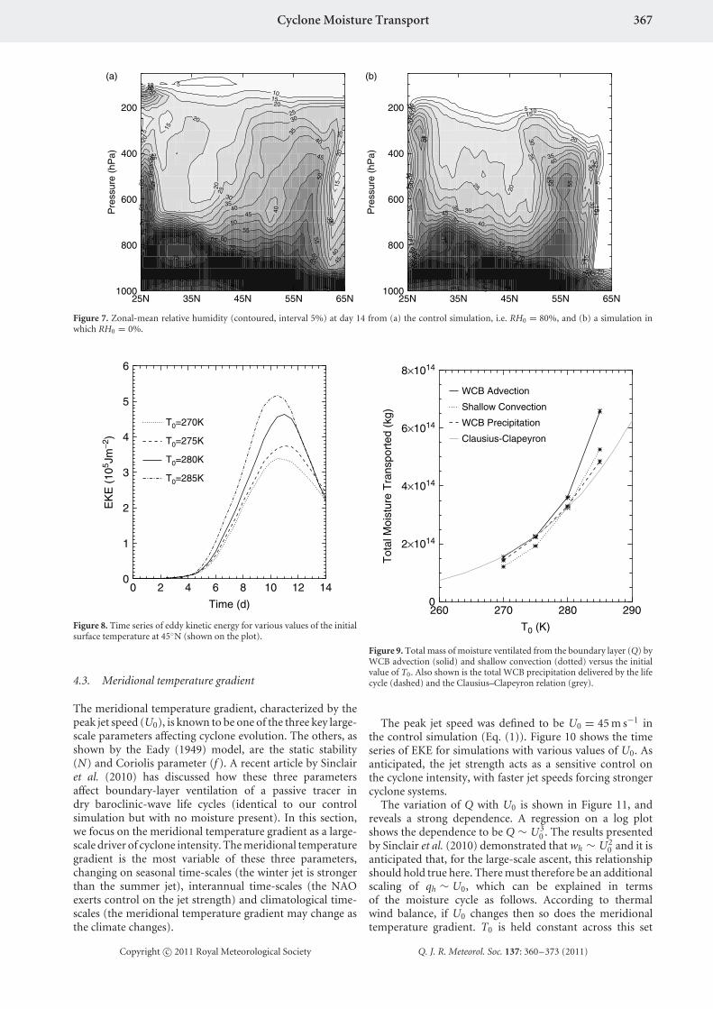
These simulations show why, for midlatitude regions,the RH profile remains approximately constant. If, for anyreason, the RH profile is moved away from its equilibriumstate, evaporation and precipitation processes driven by thelarge-scale cyclone dynamics redistribute moisture until theequilibrium state is returned. This adjustment process isfast and can happen within one cyclone life cycle. Figure 7shows the zonal-mean relative humidity from simulationsat day 14 with RH0 = 80% and 0% respectively. It can beseen that between 30–60◦N and up to 200 hPa (the regionthis cyclone system influences) the two simulations aresimilar qualitatively and even quantitatively, demonstratingthat even a single life cycle can create a profile close toclimatology. The cyclone has not produced any moisturetransport further north than 60◦N, although this is a featureof our initial conditions and differences in storm trackorientation could lead to cyclones transporting moisturefurther north. The system has also not exported any moisture

into the stratosphere, meaning other processes are importantfor this transport.

4.2. Absolute temperature

Dry simulations of cyclogenesis are not affected by theabsolute temperature of the atmosphere – only the me-ridional temperature gradient is important (see, for example,the Eady (1949) model). Section 4.1 demonstrated thatthe initial moisture content of the atmosphere does notaffect the cyclone moisture cycle to any great extent, sincethe atmosphere quickly recovers its equilibrium relativehumidity by evaporation and precipitation processes. Theabsolute temperature of the atmosphere determines thesaturation vapour pressure, and so should affect the moisturecycle and hence possibly the large-scale development of thesystem via higher latent-heat release.

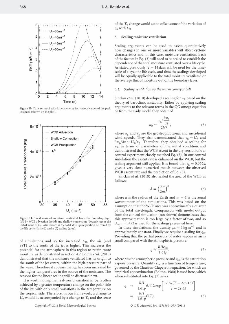
We investigate these possibilities through a series ofsimulations in which a constant value is added to orsubtracted from the atmospheric and surface-temperatureprofiles. The temperature changes will be interpreted interms of the surface temperature at 45◦N (the jet centre). Forthe control simulation, T0 = 280 K. The relative humidityprofile is fixed across all experiments and therefore thespecific humidity profile changes for each simulation,dependent on the atmospheric temperature. Figure 8 showsthe evolution of EKE for several simulations with differenttemperatures. The general trend is that a higher temperatureleads to more intense systems.

Figure 9 shows the variation of Q with T0. Asanticipated by the Clausius–Clapeyron equation, there isa strong relation between the moisture ventilated and theabsolute temperature. These results are consistent withthose presented by Allen and Ingram (2002) and Fieldand Wood (2007). Field and Wood (2007) demonstratedthat an increase of 7 K in the SST led to an approximately50% increase in precipitation rate, whilst Allen and Ingram(2002) suggested that if precipitation increased at the samerate as the global increase in atmospheric water-vapourstorage then there should be a 6.5% K−1 increase. Both ofthese quantitative predictions fit well with the observedvariation in these simulations. The variation in WCBprecipitation closely matches what would be expected fromthe Clausius–Clapeyron relation, as shown in Figure 9, whilstthe WCB advection and shallow convection have a slightlystronger variation, especially at higher temperatures. Thisis likely to be due to a positive feedback within the system– at very high temperatures, there is so much latent heatrelease that wh is increased. Examination of the modeloutput has shown that wh does show a slight increase as T0

is increased. Therefore, most of the variation in Q can beexplained by the change in qh due to Clausius–Clapeyron,and the additional variation comes from the higher valuesof wh. The precipitation efficiency of the WCB dropsslightly at higher temperatures since, although the initialRH is fixed across all simulations, the troposphere is notsaturated and can be moistened by the WCB. At highertemperatures, the increased saturation vapour pressuremeans a greater quantity of moisture can remain in thetroposphere.



25N 35N 45N 55N 65N1000

800

600

400

200P

ress

ure

(hP

a)

51010

15

15

15

15

15

20

20

20

20

20

20

25

25

25

25

25

30

30

30

30

30

35

35

35

35

40

40

40

40

40

45

45

45

45

50

50

50

55

55

55

60

60

60

65

65

65

70

70

70

75

75

7575

80 80

80

8080

(a)

25N 35N 45N 55N 65N1000

800

600

400

200

Pre

ssur

e (h

Pa)

5

5

5

10 10

10

1515

1515

2020

20

20

20

2525

25

25

25

3030

30

30

3030

35 35

35

35

40

40

40

40

40

45

45

45

45

45

50

50

50

50

55

55

55

60

60

60

6565

6570

70 70

75

75

75

75

80

80 80

(b)

Figure 7. Zonal-mean relative humidity (contoured, interval 5%) at day 14 from (a) the control simulation, i.e. RH0 = 80%, and (b) a simulation inwhich RH0 = 0%.

0 2 4 6 8 10 12 14

Time (d)

0

1

2

3

4

5

6

EK

E (

105 J

m−2

)

T0=280K

T0=270K

T0=275K

T0=285K

Figure 8. Time series of eddy kinetic energy for various values of the initialsurface temperature at 45◦N (shown on the plot).

4.3. Meridional temperature gradient

The meridional temperature gradient, characterized by thepeak jet speed (U0), is known to be one of the three key large-scale parameters affecting cyclone evolution. The others, asshown by the Eady (1949) model, are the static stability(N) and Coriolis parameter (f ). A recent article by Sinclairet al. (2010) has discussed how these three parametersaffect boundary-layer ventilation of a passive tracer indry baroclinic-wave life cycles (identical to our controlsimulation but with no moisture present). In this section,we focus on the meridional temperature gradient as a large-scale driver of cyclone intensity. The meridional temperaturegradient is the most variable of these three parameters,changing on seasonal time-scales (the winter jet is strongerthan the summer jet), interannual time-scales (the NAOexerts control on the jet strength) and climatological time-scales (the meridional temperature gradient may change asthe climate changes).

260 270 280 290

T0 (K)

0

2×1014

4×1014

6×1014

8×1014

Tot

al M

oist

ure

Tra

nspo

rted

(kg

)WCB Advection

Shallow Convection

WCB Precipitation

Clausius-Clapeyron

Figure 9. Total mass of moisture ventilated from the boundary layer (Q) byWCB advection (solid) and shallow convection (dotted) versus the initialvalue of T0. Also shown is the total WCB precipitation delivered by the lifecycle (dashed) and the Clausius–Clapeyron relation (grey).

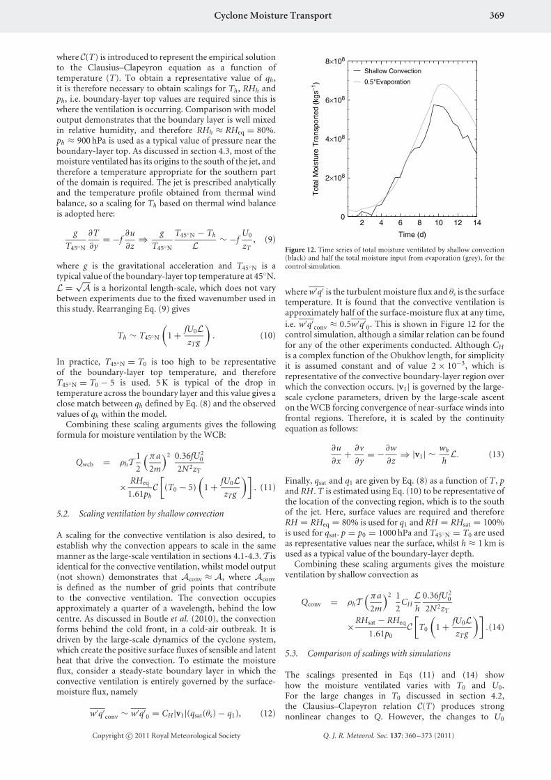
The peak jet speed was defined to be U0 = 45 m s−1 inthe control simulation (Eq. (1)). Figure 10 shows the timeseries of EKE for simulations with various values of U0. Asanticipated, the jet strength acts as a sensitive control onthe cyclone intensity, with faster jet speeds forcing strongercyclone systems.

The variation of Q with U0 is shown in Figure 11, andreveals a strong dependence. A regression on a log plotshows the dependence to be Q ∼ U3

0 . The results presentedby Sinclair et al. (2010) demonstrated that wh ∼ U2

0 and it isanticipated that, for the large-scale ascent, this relationshipshould hold true here. There must therefore be an additionalscaling of qh ∼ U0, which can be explained in termsof the moisture cycle as follows. According to thermalwind balance, if U0 changes then so does the meridionaltemperature gradient. T0 is held constant across this set



0 2 4 6 8 10 12 14

Time (d)

0

1

2

3

4

5

6

EK

E (

105 J

m−2

)

U0=45ms−1

U0=35ms−1

U0=40ms−1

U0=50ms−1

Figure 10. Time series of eddy kinetic energy for various values of the peakjet speed (shown on the plot).

30 35 40 45 50 55

U0 (ms−1)

0

2×1014

4×1014

6×1014

Tot

al M

oist

ure

Tra

nspo

rted

(kg

)

WCB Advection

Shallow Convection

WCB Precipitation

U03

Figure 11. Total mass of moisture ventilated from the boundary layer(Q) by WCB advection (solid) and shallow convection (dotted) versus theinitial value of U0. Also shown is the total WCB precipitation delivered bythe life cycle (dashed) and a U3

0 scaling (grey).

of simulations and so for increased U0, the air (andSST) to the south of the jet is higher. This increases thepotential for the atmosphere in this region to retain moremoisture, as demonstrated in section 4.2. Boutle et al. (2010)demonstrated that the moisture ventilated has its origin tothe south of the jet centre, within the high-pressure part ofthe wave. Therefore it appears that qh has been increased bythe higher temperatures in the source of the moisture. Thereasons for the linear scaling will be discussed next.

It is worth noting that real-world variation in U0 is oftenachieved by a greater temperature change on the polar sideof the jet, with only small variations in the temperature onthe tropical side. Therefore, in our framework, a change toU0 would be accompanied by a change to T0 and the sense

of the T0 change would act to offset some of the variation ofqh with U0.

5. Scaling moisture ventilation

Scaling arguments can be used to assess quantitativelyhow changes in one or more variables will affect cyclonecharacteristics and, in this case, moisture ventilation. Eachof the factors in Eq. (3) will need to be scaled to establish thedependence of the total moisture ventilated over a life cycle.As stated previously, T = 14 days will be used for the time-scale of a cyclone life cycle, and thus the scalings developedwill be equally applicable to the total moisture ventilated orthe average flux of moisture out of the boundary layer.

5.1. Scaling ventilation by the warm conveyor belt

Sinclair et al. (2010) developed a scaling for wh based on thetheory of baroclinic instability. Either by applying scalingarguments to the relevant terms in the QG omega equationor from the Eady model they obtained

wh ∼vgf

∂ug

∂z2N2

, (5)

where ug and vg are the geostrophic zonal and meridionalwind speeds. They also demonstrated that vg ∼ U0 and∂ug/∂z ∼ U0/zT . Therefore, they obtained a scaling forwh in terms of parameters of the initial condition anddemonstrated that the WCB ascent in the dry version of ourcontrol experiment closely matched Eq. (5). In our controlsimulation the ascent rate is enhanced on the WCB, but thescaling argument still applies. It is found that vg = 0.36U0

gives a very close numerical match between the observedWCB ascent rate and the prediction of Eq. (5).

Sinclair et al. (2010) also scaled the area of the WCB asfollows:

A =(πa

2m

)2, (6)

where a is the radius of the Earth and m = 6 is the zonalwavenumber of the simulations. This was based on theassumption that the WCB area was approximately a quarterof the total wavelength. Comparison with model outputfrom the control simulation (not shown) demonstrates thatthis approximation is too large by a factor of two, and soAwcb = A/2 is used for the scalings presented here.

In these simulations, the density ρh ≈ 1 kg m−3 and isapproximately constant. Finally we require a scaling for qh.Providing that the partial pressure of water vapour in air issmall compared with the atmospheric pressure,

q ≈ RHesat

1.61p, (7)

where p is the atmospheric pressure and esat is the saturationvapour pressure. Quantity esat is a function of temperature,governed by the Clausius–Clapeyron equation, for which anempirical approximation (Bolton, 1980) is used here, whichwhen substituted into Eq. (7) gives

q ≈ RH

1.61p6.112 exp

[17.67(T − 273.15)

T − 29.65

]

= RH

1.61pC(T), (8)



where C(T) is introduced to represent the empirical solutionto the Clausius–Clapeyron equation as a function oftemperature (T). To obtain a representative value of qh,it is therefore necessary to obtain scalings for Th, RHh andph, i.e. boundary-layer top values are required since this iswhere the ventilation is occurring. Comparison with modeloutput demonstrates that the boundary layer is well mixedin relative humidity, and therefore RHh ≈ RHeq = 80%.ph ≈ 900 hPa is used as a typical value of pressure near theboundary-layer top. As discussed in section 4.3, most of themoisture ventilated has its origins to the south of the jet, andtherefore a temperature appropriate for the southern partof the domain is required. The jet is prescribed analyticallyand the temperature profile obtained from thermal windbalance, so a scaling for Th based on thermal wind balanceis adopted here:

g

T45◦N

∂T

∂y= −f

∂u

∂z⇒ g

T45◦N

T45◦N − Th

L ∼ −fU0

zT, (9)

where g is the gravitational acceleration and T45◦N is atypical value of the boundary-layer top temperature at 45◦N.L = √

A is a horizontal length-scale, which does not varybetween experiments due to the fixed wavenumber used inthis study. Rearranging Eq. (9) gives

Th ∼ T45◦N

(1 + fU0L

zTg

). (10)

In practice, T45◦N = T0 is too high to be representativeof the boundary-layer top temperature, and thereforeT45◦N = T0 − 5 is used. 5 K is typical of the drop intemperature across the boundary layer and this value gives aclose match between qh defined by Eq. (8) and the observedvalues of qh within the model.

Combining these scaling arguments gives the followingformula for moisture ventilation by the WCB:

Qwcb = ρhT1

2

(πa

2m

)2 0.36fU20

2N2zT

× RHeq

1.61phC

[(T0 − 5)

(1 + fU0L

zTg

)]. (11)

5.2. Scaling ventilation by shallow convection

A scaling for the convective ventilation is also desired, toestablish why the convection appears to scale in the samemanner as the large-scale ventilation in sections 4.1-4.3. T isidentical for the convective ventilation, whilst model output(not shown) demonstrates that Aconv ≈ A, where Aconv

is defined as the number of grid points that contributeto the convective ventilation. The convection occupiesapproximately a quarter of a wavelength, behind the lowcentre. As discussed in Boutle et al. (2010), the convectionforms behind the cold front, in a cold-air outbreak. It isdriven by the large-scale dynamics of the cyclone system,which create the positive surface fluxes of sensible and latentheat that drive the convection. To estimate the moistureflux, consider a steady-state boundary layer in which theconvective ventilation is entirely governed by the surface-moisture flux, namely

w′q′conv ∼ w′q′

0 = CH|v1|(qsat(θs) − q1), (12)

2 4 6 8 10 12 14

Time (d)

0

2×108

4×108

6×108

8×108

Tot

al M

oist

ure

Tra

nspo

rted

(kg

s−1)

Shallow Convection

0.5*Evaporation

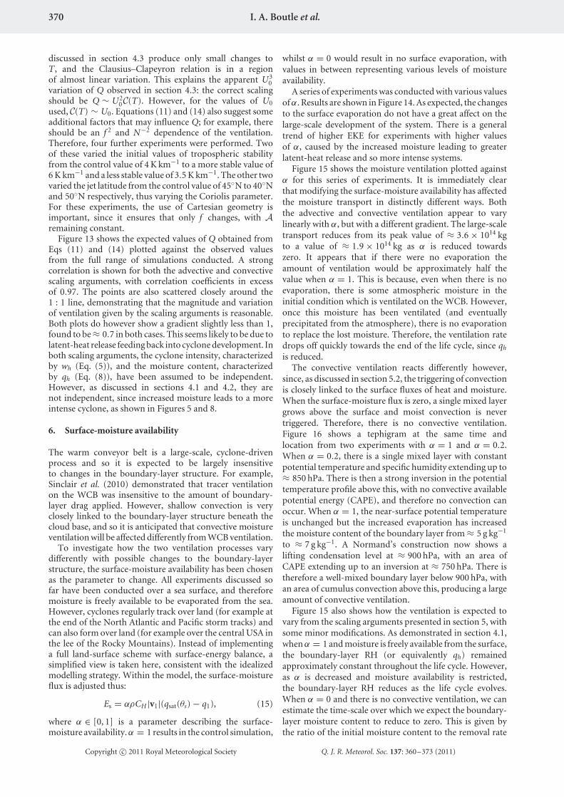
Figure 12. Time series of total moisture ventilated by shallow convection(black) and half the total moisture input from evaporation (grey), for thecontrol simulation.

where w′q′ is the turbulent moisture flux and θs is the surfacetemperature. It is found that the convective ventilation isapproximately half of the surface-moisture flux at any time,i.e. w′q′

conv ≈ 0.5w′q′0. This is shown in Figure 12 for the

control simulation, although a similar relation can be foundfor any of the other experiments conducted. Although CH

is a complex function of the Obukhov length, for simplicityit is assumed constant and of value 2 × 10−3, which isrepresentative of the convective boundary-layer region overwhich the convection occurs. |v1| is governed by the large-scale cyclone parameters, driven by the large-scale ascenton the WCB forcing convergence of near-surface winds intofrontal regions. Therefore, it is scaled by the continuityequation as follows:

∂u

∂x+ ∂v

∂y= −∂w

∂z⇒ |v1| ∼ wh

hL. (13)

Finally, qsat and q1 are given by Eq. (8) as a function of T, pand RH. T is estimated using Eq. (10) to be representative ofthe location of the convecting region, which is to the southof the jet. Here, surface values are required and thereforeRH = RHeq = 80% is used for q1 and RH = RHsat = 100%is used for qsat. p = p0 = 1000 hPa and T45◦N = T0 are usedas representative values near the surface, whilst h ≈ 1 km isused as a typical value of the boundary-layer depth.

Combining these scaling arguments gives the moistureventilation by shallow convection as

Qconv = ρhT(πa

2m

)2 1

2CH

Lh

0.36fU20

2N2zT

×RHsat − RHeq

1.61p0C

[T0

(1 + fU0L

zTg

)].(14)

5.3. Comparison of scalings with simulations

The scalings presented in Eqs (11) and (14) showhow the moisture ventilated varies with T0 and U0.For the large changes in T0 discussed in section 4.2,the Clausius–Clapeyron relation C(T) produces strongnonlinear changes to Q. However, the changes to U0



discussed in section 4.3 produce only small changes toT, and the Clausius–Clapeyron relation is in a regionof almost linear variation. This explains the apparent U3

0variation of Q observed in section 4.3: the correct scalingshould be Q ∼ U2

0C(T). However, for the values of U0

used, C(T) ∼ U0. Equations (11) and (14) also suggest someadditional factors that may influence Q; for example, thereshould be an f 2 and N−2 dependence of the ventilation.Therefore, four further experiments were performed. Twoof these varied the initial values of tropospheric stabilityfrom the control value of 4 K km−1 to a more stable value of6 K km−1 and a less stable value of 3.5 K km−1. The other twovaried the jet latitude from the control value of 45◦N to 40◦Nand 50◦N respectively, thus varying the Coriolis parameter.For these experiments, the use of Cartesian geometry isimportant, since it ensures that only f changes, with Aremaining constant.

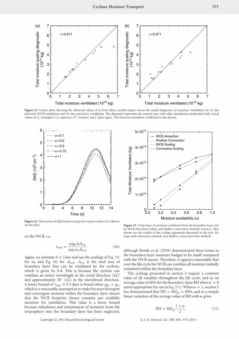
Figure 13 shows the expected values of Q obtained fromEqs (11) and (14) plotted against the observed valuesfrom the full range of simulations conducted. A strongcorrelation is shown for both the advective and convectivescaling arguments, with correlation coefficients in excessof 0.97. The points are also scattered closely around the1 : 1 line, demonstrating that the magnitude and variationof ventilation given by the scaling arguments is reasonable.Both plots do however show a gradient slightly less than 1,found to be ≈ 0.7 in both cases. This seems likely to be due tolatent-heat release feeding back into cyclone development. Inboth scaling arguments, the cyclone intensity, characterizedby wh (Eq. (5)), and the moisture content, characterizedby qh (Eq. (8)), have been assumed to be independent.However, as discussed in sections 4.1 and 4.2, they arenot independent, since increased moisture leads to a moreintense cyclone, as shown in Figures 5 and 8.

6. Surface-moisture availability

The warm conveyor belt is a large-scale, cyclone-drivenprocess and so it is expected to be largely insensitiveto changes in the boundary-layer structure. For example,Sinclair et al. (2010) demonstrated that tracer ventilationon the WCB was insensitive to the amount of boundary-layer drag applied. However, shallow convection is veryclosely linked to the boundary-layer structure beneath thecloud base, and so it is anticipated that convective moistureventilation will be affected differently from WCB ventilation.

To investigate how the two ventilation processes varydifferently with possible changes to the boundary-layerstructure, the surface-moisture availability has been chosenas the parameter to change. All experiments discussed sofar have been conducted over a sea surface, and thereforemoisture is freely available to be evaporated from the sea.However, cyclones regularly track over land (for example atthe end of the North Atlantic and Pacific storm tracks) andcan also form over land (for example over the central USA inthe lee of the Rocky Mountains). Instead of implementinga full land-surface scheme with surface-energy balance, asimplified view is taken here, consistent with the idealizedmodelling strategy. Within the model, the surface-moistureflux is adjusted thus:

Es = αρCH |v1|(qsat(θs) − q1), (15)

where α ∈ [0, 1] is a parameter describing the surface-moisture availability. α = 1 results in the control simulation,

whilst α = 0 would result in no surface evaporation, withvalues in between representing various levels of moistureavailability.

A series of experiments was conducted with various valuesof α. Results are shown in Figure 14. As expected, the changesto the surface evaporation do not have a great affect on thelarge-scale development of the system. There is a generaltrend of higher EKE for experiments with higher valuesof α, caused by the increased moisture leading to greaterlatent-heat release and so more intense systems.

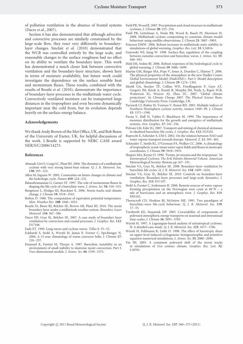
Figure 15 shows the moisture ventilation plotted againstα for this series of experiments. It is immediately clearthat modifying the surface-moisture availability has affectedthe moisture transport in distinctly different ways. Boththe advective and convective ventilation appear to varylinearly with α, but with a different gradient. The large-scaletransport reduces from its peak value of ≈ 3.6 × 1014 kgto a value of ≈ 1.9 × 1014 kg as α is reduced towardszero. It appears that if there were no evaporation theamount of ventilation would be approximately half thevalue when α = 1. This is because, even when there is noevaporation, there is some atmospheric moisture in theinitial condition which is ventilated on the WCB. However,once this moisture has been ventilated (and eventuallyprecipitated from the atmosphere), there is no evaporationto replace the lost moisture. Therefore, the ventilation ratedrops off quickly towards the end of the life cycle, since qh

is reduced.The convective ventilation reacts differently however,

since, as discussed in section 5.2, the triggering of convectionis closely linked to the surface fluxes of heat and moisture.When the surface-moisture flux is zero, a single mixed layergrows above the surface and moist convection is nevertriggered. Therefore, there is no convective ventilation.Figure 16 shows a tephigram at the same time andlocation from two experiments with α = 1 and α = 0.2.When α = 0.2, there is a single mixed layer with constantpotential temperature and specific humidity extending up to≈ 850 hPa. There is then a strong inversion in the potentialtemperature profile above this, with no convective availablepotential energy (CAPE), and therefore no convection canoccur. When α = 1, the near-surface potential temperatureis unchanged but the increased evaporation has increasedthe moisture content of the boundary layer from ≈ 5 g kg−1

to ≈ 7 g kg−1. A Normand’s construction now shows alifting condensation level at ≈ 900 hPa, with an area ofCAPE extending up to an inversion at ≈ 750 hPa. There istherefore a well-mixed boundary layer below 900 hPa, withan area of cumulus convection above this, producing a largeamount of convective ventilation.

Figure 15 also shows how the ventilation is expected tovary from the scaling arguments presented in section 5, withsome minor modifications. As demonstrated in section 4.1,when α = 1 and moisture is freely available from the surface,the boundary-layer RH (or equivalently qh) remainedapproximately constant throughout the life cycle. However,as α is decreased and moisture availability is restricted,the boundary-layer RH reduces as the life cycle evolves.When α = 0 and there is no convective ventilation, we canestimate the time-scale over which we expect the boundary-layer moisture content to reduce to zero. This is given bythe ratio of the initial moisture content to the removal rate



0 1 2 3 4 5 6 7

Total moisture ventilated (1014 kg)

0

1

2

3

4

5

6

7

Tot

al m

oist

ure

scal

ing

diag

nost

ic(1

014 k

g)

r=0.971 r=0.971

(a)

0 1 2 3 4 5 6 7

Total moisture ventilated (1014 kg)

0

1

2

3

4

5

6

7

Tot

al m

oist

ure

scal

ing

diag

nost

ic(1

014 k

g)

(b)

Figure 13. Scatter plots showing the observed values of Q from direct model output versus the scaled diagnostic of moisture ventilation for (a) theadvective WCB ventilation and (b) the convective ventilation. The diamond represents the control run, with other simulations performed with variedvalues of T0 (triangles), U0 (squares), N2 (crosses) and f (plus signs). The Pearson correlation coefficient is also shown.

0 2 4 6 8 10 12 14

Time (d)

0

1

2

3

4

5

6

EK

E (

105Jm

−2)

α=0.75

α=1

α=0.1

α=0.2

α=0.5

Figure 14. Time series of eddy kinetic energy for various values of α (shownon the plot).

on the WCB, i.e.

τrem = ρqBLhAcyc

ρqhwhAwcb. (16)

Again, we estimate h ≈ 1 km and use the scalings of Eq. (5)for wh and Eq. (6) for Awcb. Acyc is the total area ofboundary layer that can be ventilated by the cyclone,which is given by 8A. This is because the cyclone canventilate an entire wavelength in the zonal direction (4L)and approximately 30◦ (2L) in the meridional direction.A lower bound of τrem ≈ 9.5 days is found when qBL = qh,which is a reasonable assumption to make because divergentand convergent motions within the boundary layer ensurethat the WCB footprint always contains any availablemoisture for ventilation. This value is a lower boundbecause subsidence and entrainment of moisture from thetroposphere into the boundary layer has been neglected,

0.0 0.2 0.4 0.6 0.8 1.0

Moisture availability (α)

0

1×1014

2×1014

3×1014

4×1014

5×1014T

otal

Moi

stur

e V

entil

ated

(kg

)

WCB AdvectionShallow ConvectionWCB ScalingConvective Scaling

Figure 15. Total mass of moisture ventilated from the boundary layer (Q)by WCB advection (solid) and shallow convection (dotted) versus α. Alsoshown are the results of the scaling arguments discussed in the text, forlarge-scale advection (dashed) and shallow convection (dot–dashed).

although Boutle et al. (2010) demonstrated these terms inthe boundary-layer moisture budget to be small comparedwith the WCB ascent. Therefore, it appears reasonable thatover the life cycle the WCB can ventilate all moisture initiallycontained within the boundary layer.

The scalings presented in section 5 require a constantvalue of all variables throughout the life cycle, and so anaverage value of 40% for the boundary-layer RH when α = 0seems appropriate for use in Eq. (11). When α = 1, section 5has demonstrated that RH = RHeq = 80%, and so a simplelinear variation of the average value of RH with α gives

RH = RHeq1 + α

2, (17)



Figure 16. Tephigram in the shallow convective region (−27.6◦E, 36.8◦N)at day 7, showing experiments with α = 1 (solid) and α = 0.2 (dashed).

which is used in Eq. (11) and gives good agreement with themeasured values of Qwcb in Figure 15.

Section 5.2 discussed how the convective ventilation isproportional to the surface-moisture flux, and thereforethe scaling for convective ventilation, given in Eq. (12), ismodified thus:

w′q′conv ∼ αCH|v1|(qsat(θs) − q1). (18)

This introduces a factor of α into Eq. (14), and Figure 15also shows this scaling to be in good agreement with theobserved values of Qconv.

7. Conclusions

This article has shown from a combination of numericalexperiments and simple scaling arguments how boundary-layer moisture ventilation varies with changes to large-scaleand boundary-layer parameters. Whilst results and scalingarguments have typically been presented in terms of themoisture ventilated from the boundary layer, it is importantto note that moisture transport can be thought of as a proxyfor many other processes. Boutle et al. (2010) demonstratedhow the large-scale ventilation on the WCB was balancedby a convergence of moisture within the boundary layer,which is, in turn, balanced by divergence of moisturefrom anticyclonic regions of the baroclinic wave. It wasalso discussed how the WCB is close to 100% efficient atconverting ascending moisture into precipitation (Eckhardtet al., 2004), and therefore the scalings presented for WCBventilation also describe how the WCB precipitation is likelyto vary.

A strong dependence of the moisture transport on thejet strength has been demonstrated, with Q ∼ U3

0 . This isin good agreement with the results of Stohl et al. (2008),who demonstrate a strong dependence of poleward moisturetransport and precipitation on the NAO. A positive NAOcauses increased jet strength, and so the U3

0 scaling showswhy there is such a strong variation with the NAO. Ruprecht

et al. (2002) also demonstrated increased moisture transportin positive NAO conditions due to the poleward shift inthe jet, which has also been demonstrated from scalingarguments, with Q ∼ f 2. It is worth noting that in both ofthese circumstances there is likely to be some offsetting tothe moisture transport from a reduction in T0, and that theorientation of the jet may change with the NAO, an effectthat has not been considered here.

Field and Wood (2007) argued for a scaling of the WCBrain rate as follows:

Rwcb = c〈V〉〈WVP〉, (19)

where c depends on the cyclone area, the size of the WCBinflow and the asymmetry in moisture distribution withinthe cyclone. The scaling arguments presented here havedemonstrated consistency with this scaling. It has beenshown here that

Rwcb = cwhqh, (20)

where continuity implies 〈V〉 ∼ wh, whilst 〈WVP〉 ∼ qh

since most moisture is contained within the boundary layerand so the effect of free-tropospheric moisture, includedin 〈WVP〉, is small. c incorporates these proportionalityrelations and c. It has been shown here why qh variesaccording to the Clausius–Clapeyron equation, a fact notedin Field and Wood (2007).

The scaling arguments also provide an interestingframework for interpreting climate model results. Forexample, it is anticipated that polar regions will warmfaster than equatorial regions (Meehl et al., 2007), there willbe a poleward shift in the storm track (Yin, 2005) and anincrease in midlatitude static stability (Frierson, 2006). Theresponse of cyclone moisture transport and precipitation istherefore a complicated combination of these changes. Thescalings suggests that increased global mean temperaturewill increase the moisture transport, but this could be offsetby a reduction in the meridional temperature gradient (dueto the polar regions warming faster). The poleward shiftin the storm tracks should provide another mechanismfor increased moisture transport, but this could again beoffset by an increase in static stability. Therefore, even thesign of the midlatitude moisture transport and precipitationresponse is a complex combination of the magnitude ofchanges to several other variables, and whilst it seems likelythat there will be an overall increase in midlatitude moisturetransport (Held and Soden, 2006), the precise mechanismfor this is unclear. Recent trends suggest that the frequency ofcyclones is reducing (Paciorek et al., 2002). Therefore, eachsystem will require a larger increase in moisture transport(and precipitation) than the midlatitude mean to accountfor the reduced number of storms.

The scaling arguments have demonstrated the key physicalvariables that influence cyclone moisture transport andprecipitation, but they also have many other potentialuses. Their simplicity means that they can be usedfor climatological studies of moisture transport andprecipitation and also for pollution ventilation with someminor modification. Sinclair et al. (2010) discussed how thelarge-scale advection could be used to create pollution-ventilation climatologies. The present work provides asimilar scaling for ventilation by moist convection, a processthat has been previously shown to be an efficient method



of pollution ventilation in the absence of frontal systems(Dacre et al., 2007).

Section 6 has also demonstrated that although advectiveand convective processes are similarly constrained by thelarge-scale flow, they react very differently to boundary-layer changes. Sinclair et al. (2010) demonstrated thatthe WCB was controlled entirely by the large scale, andreasonable changes to the surface roughness had no effecton its ability to ventilate the boundary layer. This workhas demonstrated a much closer link between convectiveventilation and the boundary-layer structure, shown herein terms of moisture availability, but future work couldinvestigate the dependence on the surface sensible heatand momentum fluxes. These results, combined with theresults of Boutle et al. (2010), demonstrate the importanceof boundary-layer processes to the midlatitude water cycle.Convectively ventilated moisture can be transported largedistances in the troposphere and even become dynamicallyimportant near the cold front, but its evolution dependsheavily on the surface-energy balance.

Acknowledgements

We thank Andy Brown of the Met Office, UK, and Bob Beareof the University of Exeter, UK, for helpful discussions ofthe work. I. Boutle is supported by NERC CASE awardNER/S/C/2006/14273.

References

Ahmadi-Givi F, Craig GC, Plant RS. 2004. The dynamics of a midlatitudecyclone with very strong latent-heat release. Q. J. R. Meteorol. Soc.130: 295–323.

Allen M, Ingram W. 2002. Constraints on future changes in climate andthe hydrologic cycle. Nature 419: 224–232.

Balasubramanian G, Garner ST. 1997. The role of momentum fluxes inshaping the life cycle of a baroclinic wave. J. Atmos. Sci. 54: 510–533.

Bengtsson L, Hodges KI, Roeckner E. 2006. Storm tracks and climatechange. J. Climate 19: 3518–3543.

Bolton D. 1980. The computation of equivalent potential temperature.Mon. Weather Rev. 108: 1046–1053.

Boutle IA, Beare RJ, Belcher SE, Brown AR, Plant RS. 2010. The moistboundary layer under a midlatitude weather system. Boundary-LayerMeteorol. 134: 367–386.

Dacre HF, Gray SL, Belcher SE. 2007. A case study of boundary layerventilation by convection and coastal processes. J. Geophys. Res. 112:D17106.

Eady ET. 1949. Long waves and cyclone waves. Tellus 1: 33–52.Eckhardt S, Stohl A, Wernli H, James P, Forster C, Spichtinger N.

2004. A 15-year climatology of warm conveyor belts. J. Climate 17:218–237.

Emanuel K, Fantini M, Thorpe A. 1987. Baroclinic instability in anenvironment of small stability to slantwise moist convection. Part I:Two-dimensional models. J. Atmos. Sci. 44: 1559–1573.

Field PR, Wood R. 2007. Precipitation and cloud structure in midlatitudecyclones. J. Climate 20: 233–254.

Field PR, Gettelman A, Neale RB, Wood R, Rasch PJ, Morrison H.2008. Midlatitude cyclone compositing to constrain climate modelbehaviour using satellite observations. J. Climate 21: 5887–5903.

Frierson DMW. 2006. Robust increases in midlatitude static stability insimulations of global warming. Geophys. Res. Lett. 33: L24816.

Gutowski WJ, Jiang W. 1998. Surface-flux regulation of the couplingbetween cumulus convection and baroclinic waves. J. Atmos. Sci. 55:940–953.

Held IM, Soden BJ. 2006. Robust responses of the hydrological cycle toglobal warming. J. Climate 19: 5686–5699.

Martin GM, Ringer MA, Pope V, Jones A, Dearden C, Hinton T. 2006.The physical properties of the atmosphere in the new Hadley CentreGlobal Environment Model (HadGEM1). Part I: Model descriptionand global climatology. J. Climate 19: 1274–1301.

Meehl GA, Stocker TF, Collins WD, Friedlingstein P, Gaye AT,Gregory JM, Kitoh A, Knutti R, Murphy JM, Noda A, Raper SCB,Watterson IG, Weaver AJ, Zhao ZC. 2007. ‘Global climateprojections’. In Climate Change 2007: The Physical Science Basis.Cambridge University Press: Cambridge, UK.

Paciorek CJ, Risbey JS, Ventura V, Rosen RD. 2002. Multiple indices ofNorthern Hemisphere cyclone activity, winters 1949–99. J. Climate15: 1573–1590.

Pavan V, Hall N, Valdes P, Blackburn M. 1999. The importance ofmoisture distribution for the growth and energetics of midlatitudesystems. Ann. Geophys. 17: 242–256.

Polvani LM, Esler JG. 2007. Transport and mixing of chemical airmassesin idealized baroclinic life cycles. J. Geophys. Res. 112: D23102.

Ruprecht E, Schroder S, Ubl S. 2002. On the relation between NAO andwater vapour transport towards Europe. Meteorol. Z. 11: 395–401.

Schneider T, Smith KL, O’Gorman PA, Walker CC. 2006. A climatologyof tropospheric zonal-mean water vapor fields and fluxes in isentropiccoordinates. J. Climate 19: 5918–5933.

Shapiro MA, Keyser D. 1990. ‘Fronts, jet streams and the tropopause’. InExtratropical Cyclones: The Erik Palmen Memorial Volume. AmericanMeteorological Society: Boston; pp 167–191.

Sinclair VA, Gray SL, Belcher SE. 2008. Boundary-layer ventilation bybaroclinic life cycles. Q. J. R. Meteorol. Soc. 134: 1409–1424.

Sinclair VA, Gray SL, Belcher SE. 2010. Controls on boundary-layerventilation: Boundary-layer processes and large-scale dynamics. J.Geophys. Res. 115: D11107.

Stohl A, Forster C, Sodemann H. 2008. Remote sources of water vapourforming precipitation on the Norwegian west coast at 60◦N – atale of hurricanes and an atmospheric river. J. Geophys. Res. 113:D05102.

Thorncroft CD, Hoskins BJ, McIntyre ME. 1993. Two paradigms ofbaroclinic-wave life-cycle behaviour. Q. J. R. Meteorol. Soc. 119:17–55.

Trenberth KE, Stepaniak DP. 2003. Covariability of components ofpoleward atmospheric energy transports on seasonal and interannualtime-scales. J. Climate 16: 3691–3705.

Wernli H. 1997. A Lagrangian-based analysis of extratropical cyclones.II: A detailed case-study. Q. J. R. Meteorol. Soc. 123: 1677–1706.

Wernli H, Fehlmann R, Luthi D. 1998. The effect of barotropic shearon upper-level induced cyclogenesis: Semigeostrophic and primitiveequation numerical simulations. J. Atmos. Sci. 55: 2080–2094.

Yin JH. 2005. A consistent poleward shift of the storm tracksin simulations of 21st century climate. Geophys. Res. Lett. 32:L18701.


Documents

Moisture transport in midlatitude cyclones - CentAURcentaur.reading.ac.uk/19144/3/783_ftp.pdf · Moisture transport in midlatitude cyclones ... Moisturetransportinmidlatitudecyclones