Embed Size (px)
Citation preview
The Effects of Monetary Policy Shocks onExchange Rates: A Structural Vector Error
Correction Model Approach
Kyungho Jang∗
Masao Ogaki†
The Ohio State University
March 1, 2001
Ohio State UniversityDepartment of EconomicsWorking Paper No. 01-02
ABSTRACT
This paper investigates the effects of shocks to U.S. monetary policy on the dollar/yenexchange rate, using structural Vector Error Correction Model (VECM) methods.We compare our estimates of the impulse responses with those based on levels VectorAutoregression. We also compare results from short run and long run restrictions im-posed on the structural VECM. We find evidence of overshooting behavior of exchangerates with all methods. We find the price puzzle with levels Vector Autoregressionand VECM with short-run restrictions. In contrast, we do not find the price puzzlewith VECM with long-run restrictions.
Keywords: Vector Error Correction Model, Impulse Response, Monetary Policy Shock,Cointegration, Indentification, Long Run RestrictionJEL Classification: E32, C32
∗Ohio State University, Department of Economics, Columbus OH 43210. Tel. (614) 292-9487E-mail: [email protected].
†Ohio State University, Department of Economics, Columbus OH 43210. Tel: (614) 292-5842,Fax: (614) 292-3906, E-mail: [email protected].∗† We thank Charles Evans for providing us with the data for this study, Steve Cecchetti, Paul
Evans, Pok-Sang Lam, Nelson Mark, and seminar participants at the Bank of Japan, InternationalUniversity of Japan, Kobe University, Kyoto University, and Tezukayama University for comments.

1 Introduction
This paper examines the effects of shocks to U.S. monetary policy on the dol-
lar/yen exchange rate, using structural Vector Error Correction Model (VECM) meth-
ods. We compare our estimates of the effects with those of Eichenbaum and Evans
(1995) based on levels Vector Autoregression (VAR). We also compare results from
short-run and long-run restrictions imposed on the structural VECM.
The standard exchange rate model (see, e.g., Dornbusch, 1976) predicts that
a contractionary shock to U.S. monetary policy leads to appreciation in U.S. nomi-
nal and real exchange rates. However, empirical evidence for two important building
blocks of the model is mixed at best. These two building blocks are Uncovered Interest
Parity (UIP) and long-run Purchasing Power Parity (PPP). Therefore, it is not obvi-
ous whether or not this prediction of the model holds true in the data. Eichenbaum
and Evans (1995) directly investigate this prediction by estimating impulse responses
to U.S. monetary shocks and find evidence in favor of the prediction, even though
their results do not support some aspects of the standard exchange rate model.
In order to investigate the impulse responses to a monetary policy shock, it is
necessary to identify the shock by imposing economic restrictions on an econometric
model. When economic restrictions are imposed, the econometric model is called a
structural model. Both the choice of the econometric model and the choice of the set
of restrictions can affect the point estimates and standard errors of impulse responses.
For this reason, it is important to study how these choices affect the results.
Most variables used to study exchange rate models are persistent, and usually
modeled as series with stochastic trends and cointegration. In such a case, both
levels VAR and VECM can be used to estimate impulse responses. Levels VAR is
1
more robust than VECM because it can be used even when the system does not
have stochastic trends and cointegration. Perhaps for this reason, it is used in most
studies of impulse responses and by Eichenbaum and Evans (1995). However, struc-
tural VECM has some important advantages in systems with stochastic trends and
cointegration. First, other things being equal, estimators of impulse responses from
structural VECM are more precise. For example, levels VAR can lead to explod-
ing impulse response estimates even when the true impulse response is not exploding.
This possibility is practically eliminated with structural VECM. Second, it is possible
to impose long-run restrictions as well as short-run restrictions to identify shocks.
A method of imposing long-run restrictions on VECM is developed in King,
Plosser, Stock and Watson (1991, KPSW for short). This paper employs Jang’s
(2000) method rather than the KPSW method. Compared to the KPSW method,
Jang’s method has an advantage in that it requires neither identification nor esti-
mation of cointegrating vectors. This greatly faciliates the impulse response analysis
because identification assumptions for cointegrating vectors can be complicated, and
may be inconsistent with some long-run restrictions a researcher wishes to impose to
identify shocks. Another feature of Jang’s method is that it applies block recursive
assumptions to structural VECM with long run restrictions. The block recursive sys-
tem has been well developed in structural VAR and structural VECM with short run
restrictions, yet is not studied in the structural VECM with long run restrictions.
The identification scheme of one permanent shock in structural VECM with long run
restrictions is first developed, to our knowledge, by Jang(2000), and it is applicable
with minimal assumptions when impulse responses to only one permanent shock are
of interest.
2
2 Long run restrictions on Error Correction Models
When economic variables are cointegrated I(1) processes, the system has a
reduced rank and there exists an error correction model according to the Granger
representation theorem (see, Engle and Granger, 1987). Johansen (1988) develops
maximum likelihood estimators of cointegrating vectors and provides a rank test to
determine the number of cointegrating vectors, r.
The estimation method developed in this paper differs from the Johansen method
in the sense that i)long run restrictions are imposed on an error correction model,
ii)long run impulse response analysis is of interest, but not estimation of cointegrating
vectors.
The paper adopts the standard notation as following: i) xt is a n× 1 vector of
nonstationary variables which are assumed to be cointegrated, ii) r is the number of
cointegrating vectors, iii) k is the number of common trends, k = n− r, iv) the data
generating process is also assumed to be VAR(p) in which p is the lag length, and v)
L is the lag operator.
2.1 Error Correction Models
Suppose that xt has a finite order unrestricted VAR representation:
A(L)xt = µ + εt (2.1)
where A(L) = In −∑p
i=1 AiLi, A(0) = In, and εt is white noise with mean zero and
variance Σ. From the reduced form VAR, A(L) can be reparameterized as A(1)L +
A∗(L)(1−L) where A(1) has a reduced rank, r < n. Engle and Granger (1987) show
3
that there exists an error correction representation:
A∗(L)∆xt = µ− A(1)xt−1 + εt (2.2)
where A∗(L) = In −∑p−1
i=1 A∗i L
i, and A∗i = −∑p
j=i+1 Aj. Since xt is assumed to be
cointegrated I(1), ∆xt is I(0), and −A(1) can be decomposed as αβ′ where α and β
are n× r matrices with full column rank r.
2.2 Long run restrictions
As ∆xt is assumed to be stationary, it has a unique Wold representation:
∆xt = δ + C(L)εt (2.3)
where δ = C(1)µ, C(L) = In+∑∞
i=1 CiLi. The above reduced form can be represented
as a structural form:
∆xt = δ + Γ(L)vt
Γ(L) = C(L)Γ0 (2.4)
vt = Γ−10 εt
where Γ(L) = Γ0 +∑∞
i=1 ΓiLi, and vt is a vector of structural disturbances with mean
zero and variance Σv.
Long run restrictions are imposed on the structural form as in Blanchard and
Quah (1989, BQ for short). Stock and Watson (1988) develop a common trend repre-
sentation showing that it is equivalent to an ECM representation. When cointegrated
variables have a reduced rank r, there exist k = n − r common trends. These com-
mon trends can be considered to be generated by permanent shocks so that vt can be
decomposed into (vk′t , vr′
t )′, where vkt is a k dimensional vector of permanent shocks
4
and vrt is an r dimensional vector of transitory shocks. As developed in KPSW, this
decomposition ensures that
Γ(1) =[
A 0]
, (2.5)
where A is an n× k matrix and 0 is a n× r matrix with zeros representing long run
effects of permanent shocks and transitory shocks, respectively.
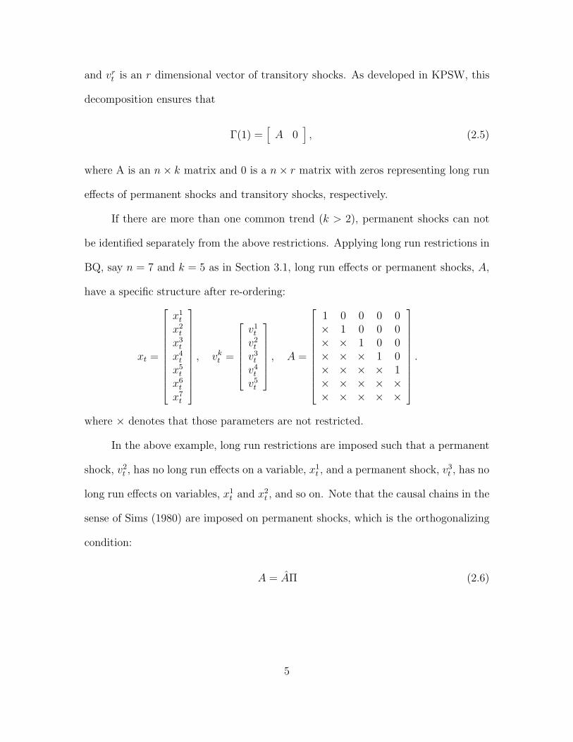
If there are more than one common trend (k > 2), permanent shocks can not
be identified separately from the above restrictions. Applying long run restrictions in
BQ, say n = 7 and k = 5 as in Section 3.1, long run effects or permanent shocks, A,
have a specific structure after re-ordering:
xt =
x1t
x2t
x3t
x4t
x5t
x6t
x7t
, vkt =
v1t
v2t
v3t
v4t
v5t
, A =
1 0 0 0 0× 1 0 0 0× × 1 0 0× × × 1 0× × × × 1× × × × ×× × × × ×
.
where × denotes that those parameters are not restricted.
In the above example, long run restrictions are imposed such that a permanent
shock, v2t , has no long run effects on a variable, x1
t , and a permanent shock, v3t , has no
long run effects on variables, x1t and x2
t , and so on. Note that the causal chains in the
sense of Sims (1980) are imposed on permanent shocks, which is the orthogonalizing
condition:
A = AΠ (2.6)
5
where A is an n × k matrix, and Π is a k × k lower triangular matrix with ones on
the diagonal. Continuing the above example, Π has the following specific form:
Π =
1 0 0 0 0π21 1 0 0 0π31 π32 1 0 0π41 π42 π43 1 0π51 π52 π53 π54 1
.
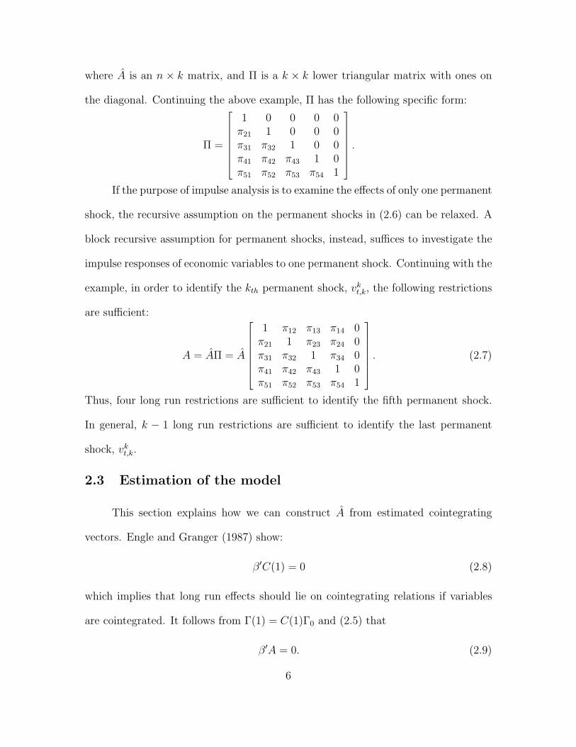
If the purpose of impulse analysis is to examine the effects of only one permanent
shock, the recursive assumption on the permanent shocks in (2.6) can be relaxed. A
block recursive assumption for permanent shocks, instead, suffices to investigate the
impulse responses of economic variables to one permanent shock. Continuing with the
example, in order to identify the kth permanent shock, vkt,k, the following restrictions
are sufficient:
A = AΠ = A
1 π12 π13 π14 0π21 1 π23 π24 0π31 π32 1 π34 0π41 π42 π43 1 0π51 π52 π53 π54 1
. (2.7)
Thus, four long run restrictions are sufficient to identify the fifth permanent shock.
In general, k − 1 long run restrictions are sufficient to identify the last permanent
shock, vkt,k.
2.3 Estimation of the model
This section explains how we can construct A from estimated cointegrating
vectors. Engle and Granger (1987) show:
β′C(1) = 0 (2.8)
which implies that long run effects should lie on cointegrating relations if variables
are cointegrated. It follows from Γ(1) = C(1)Γ0 and (2.5) that
β′A = 0. (2.9)
6
Let β⊥ be a n × k orthogonal matrix of cointegrating vectors, β, which satisfies
β′β⊥ = 0. Johansen (1995) proposes one method for choosing β⊥:
β⊥ = (In − S(β′S)−1β′)S⊥ (2.10)
where S is an n × r selection matrix, (Ir 0)′, and S⊥ is an n × k selection matrix,
(0 Ik)′.
In order to maintain BQ-type long run restrictions, one should normalize β⊥
so that some parts of the matrix contain a k × k identity matrix. Let β⊥ be the
normalized orthogonal matrix of cointegrating vectors. From A = AΠ, we can choose
the matrix:1
A = β⊥ (2.11)
Consider the seven-variable model with long run restrictions in Section 3.1. Let xt be
(yt, pt, yfort , rfor
t , rt,mt, ert )′, in which yt is output in the U.S., pt is a price level, yfor
t
is output in the foreign country, rfort is an interest rate in the foreign country, rt is
the federal funds rate, mt is a monetary variable, and ert is a real exchange rate. If
it is solely of interest to analyze the responses to a monetary policy shock, one can
impose minimal restrictions on the model. Suppose that the monetary shock does
not affect the real variables, but affects the level of U.S. price in the long run.2 These
1KPSW, instead, assume that A is known a priori, which is estimated by dynamic OLS in eachcointegrating equation.
2Note that we impose four long run restrictions in this example.
7
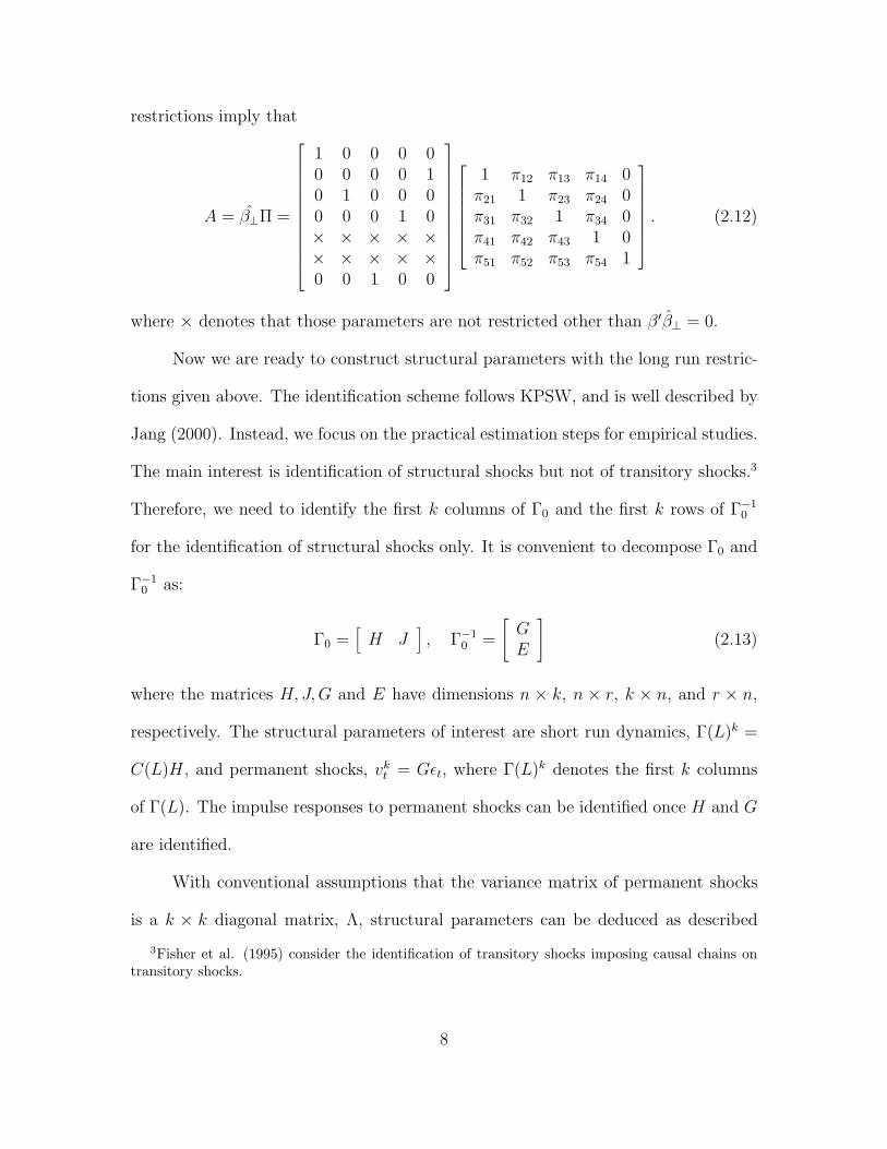
restrictions imply that
A = β⊥Π =
1 0 0 0 00 0 0 0 10 1 0 0 00 0 0 1 0× × × × ×× × × × ×0 0 1 0 0
1 π12 π13 π14 0π21 1 π23 π24 0π31 π32 1 π34 0π41 π42 π43 1 0π51 π52 π53 π54 1
. (2.12)
where × denotes that those parameters are not restricted other than β′β⊥ = 0.
Now we are ready to construct structural parameters with the long run restric-
tions given above. The identification scheme follows KPSW, and is well described by
Jang (2000). Instead, we focus on the practical estimation steps for empirical studies.
The main interest is identification of structural shocks but not of transitory shocks.3
Therefore, we need to identify the first k columns of Γ0 and the first k rows of Γ−10
for the identification of structural shocks only. It is convenient to decompose Γ0 and
Γ−10 as:
Γ0 =[
H J]
, Γ−10 =
[
GE
]
(2.13)
where the matrices H, J,G and E have dimensions n × k, n × r, k × n, and r × n,
respectively. The structural parameters of interest are short run dynamics, Γ(L)k =
C(L)H, and permanent shocks, vkt = Gεt, where Γ(L)k denotes the first k columns
of Γ(L). The impulse responses to permanent shocks can be identified once H and G
are identified.
With conventional assumptions that the variance matrix of permanent shocks
is a k × k diagonal matrix, Λ, structural parameters can be deduced as described
3Fisher et al. (1995) consider the identification of transitory shocks imposing causal chains ontransitory shocks.
8
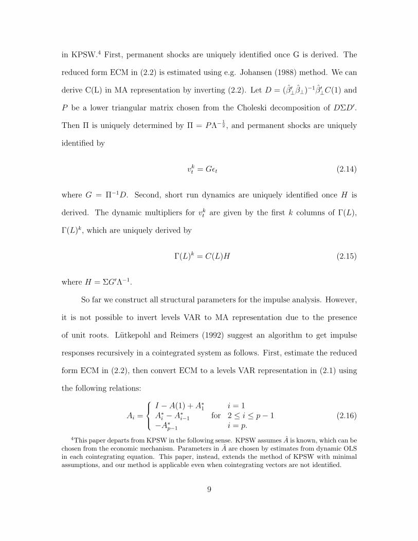
in KPSW.4 First, permanent shocks are uniquely identified once G is derived. The
reduced form ECM in (2.2) is estimated using e.g. Johansen (1988) method. We can
derive C(L) in MA representation by inverting (2.2). Let D = (β′⊥β⊥)−1β′⊥C(1) and
P be a lower triangular matrix chosen from the Choleski decomposition of DΣD′.
Then Π is uniquely determined by Π = PΛ−12 , and permanent shocks are uniquely
identified by
vkt = Gεt (2.14)
where G = Π−1D. Second, short run dynamics are uniquely identified once H is
derived. The dynamic multipliers for vkt are given by the first k columns of Γ(L),
Γ(L)k, which are uniquely derived by
Γ(L)k = C(L)H (2.15)
where H = ΣG′Λ−1.
So far we construct all structural parameters for the impulse analysis. However,
it is not possible to invert levels VAR to MA representation due to the presence
of unit roots. Lutkepohl and Reimers (1992) suggest an algorithm to get impulse
responses recursively in a cointegrated system as follows. First, estimate the reduced
form ECM in (2.2), then convert ECM to a levels VAR representation in (2.1) using
the following relations:
Ai =
I − A(1) + A∗1 i = 1
A∗i − A∗
i−1 for 2 ≤ i ≤ p− 1−A∗
p−1 i = p.(2.16)
4This paper departs from KPSW in the following sense. KPSW assumes A is known, which can bechosen from the economic mechanism. Parameters in A are chosen by estimates from dynamic OLSin each cointegrating equation. This paper, instead, extends the method of KPSW with minimalassumptions, and our method is applicable even when cointegrating vectors are not identified.
9
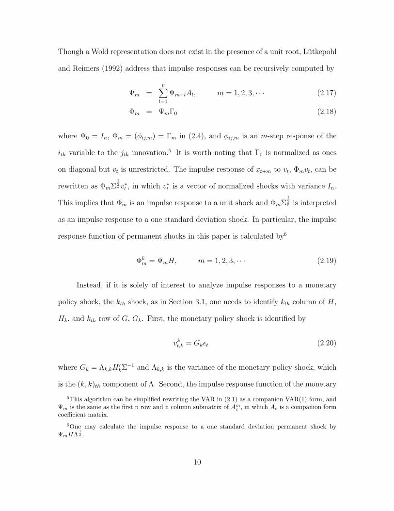
Though a Wold representation does not exist in the presence of a unit root, Lutkepohl
and Reimers (1992) address that impulse responses can be recursively computed by
Ψm =p
∑
l=1
Ψm−lAl, m = 1, 2, 3, · · · (2.17)
Φm = ΨmΓ0 (2.18)
where Ψ0 = In, Φm = (φij,m) = Γm in (2.4), and φij,m is an m-step response of the
ith variable to the jth innovation.5 It is worth noting that Γ0 is normalized as ones
on diagonal but vt is unrestricted. The impulse response of xt+m to vt, Φmvt, can be
rewritten as ΦmΣ12v v∗t , in which v∗t is a vector of normalized shocks with variance In.
This implies that Φm is an impulse response to a unit shock and ΦmΣ12v is interpreted
as an impulse response to a one standard deviation shock. In particular, the impulse
response function of permanent shocks in this paper is calculated by6
Φkm = ΨmH, m = 1, 2, 3, · · · (2.19)
Instead, if it is solely of interest to analyze impulse responses to a monetary
policy shock, the kth shock, as in Section 3.1, one needs to identify kth column of H,
Hk, and kth row of G, Gk. First, the monetary policy shock is identified by
vkt,k = Gkεt (2.20)
where Gk = Λk,kH ′kΣ
−1 and Λk,k is the variance of the monetary policy shock, which
is the (k, k)th component of Λ. Second, the impulse response function of the monetary
5This algorithm can be simplified rewriting the VAR in (2.1) as a companion VAR(1) form, andΨm is the same as the first n row and n column submatrix of Am
c , in which Ac is a companion formcoefficient matrix.
6One may calculate the impulse response to a one standard deviation permanent shock byΨmHΛ
12 .
10
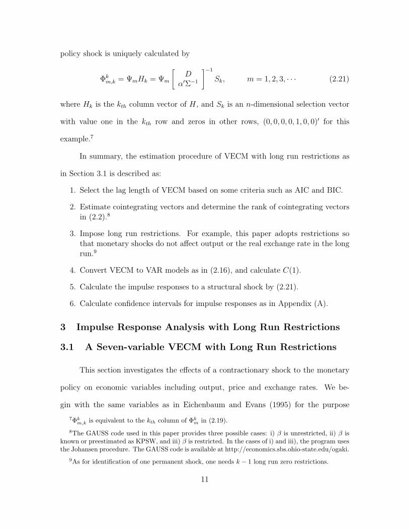
policy shock is uniquely calculated by
Φkm,k = ΨmHk = Ψm
[
Dα′Σ−1
]−1
Sk, m = 1, 2, 3, · · · (2.21)
where Hk is the kth column vector of H, and Sk is an n-dimensional selection vector
with value one in the kth row and zeros in other rows, (0, 0, 0, 0, 1, 0, 0)′ for this
example.7
In summary, the estimation procedure of VECM with long run restrictions as
in Section 3.1 is described as:
1. Select the lag length of VECM based on some criteria such as AIC and BIC.
2. Estimate cointegrating vectors and determine the rank of cointegrating vectorsin (2.2).8
3. Impose long run restrictions. For example, this paper adopts restrictions sothat monetary shocks do not affect output or the real exchange rate in the longrun.9
4. Convert VECM to VAR models as in (2.16), and calculate C(1).
5. Calculate the impulse responses to a structural shock by (2.21).
6. Calculate confidence intervals for impulse responses as in Appendix (A).
3 Impulse Response Analysis with Long Run Restrictions
3.1 A Seven-variable VECM with Long Run Restrictions
This section investigates the effects of a contractionary shock to the monetary
policy on economic variables including output, price and exchange rates. We be-
gin with the same variables as in Eichenbaum and Evans (1995) for the purpose
7Φkm,k is equivalent to the kth column of Φk
m in (2.19).
8The GAUSS code used in this paper provides three possible cases: i) β is unrestricted, ii) β isknown or preestimated as KPSW, and iii) β is restricted. In the cases of i) and iii), the program usesthe Johansen procedure. The GAUSS code is available at http://economics.sbs.ohio-state.edu/ogaki.
9As for identification of one permanent shock, one needs k − 1 long run zero restrictions.
11
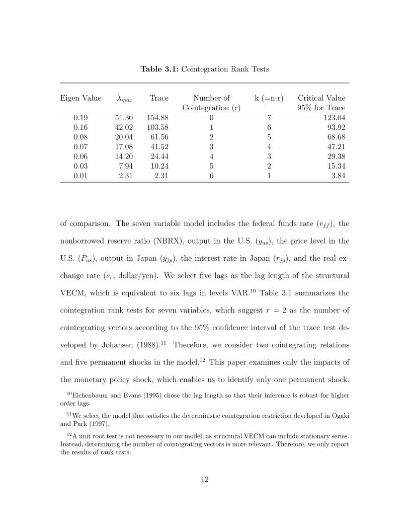
Table 3.1: Cointegration Rank Tests
Eigen Value λmax Trace Number of k (=n-r) Critical ValueCointegration (r) 95% for Trace
0.19 51.30 154.88 0 7 123.040.16 42.02 103.58 1 6 93.920.08 20.04 61.56 2 5 68.680.07 17.08 41.52 3 4 47.210.06 14.20 24.44 4 3 29.380.03 7.94 10.24 5 2 15.340.01 2.31 2.31 6 1 3.84
of comparison. The seven variable model includes the federal funds rate (rff ), the
nonborrowed reserve ratio (NBRX), output in the U.S. (yus), the price level in the
U.S. (Pus), output in Japan (yjp), the interest rate in Japan (rjp), and the real ex-
change rate (er, dollar/yen). We select five lags as the lag length of the structural
VECM, which is equivalent to six lags in levels VAR.10 Table 3.1 summarizes the
cointegration rank tests for seven variables, which suggest r = 2 as the number of
cointegrating vectors according to the 95% confidence interval of the trace test de-
veloped by Johansen (1988).11 Therefore, we consider two cointegrating relations
and five permanent shocks in the model.12 This paper examines only the impacts of
the monetary policy shock, which enables us to identify only one permanent shock.
10Eichenbaum and Evans (1995) chose the lag length so that their inference is robust for higherorder lags.
11We select the model that satisfies the deterministic cointegration restriction developed in Ogakiand Park (1997).
12A unit root test is not necessary in our model, as structural VECM can include stationary series.Instead, determining the number of cointegrating vectors is more relevant. Therefore, we only reportthe results of rank tests.
12
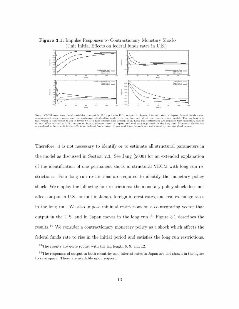
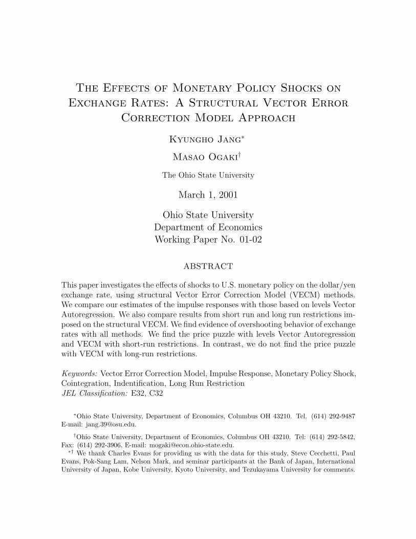
Figure 3.1: Impulse Responses to Contractionary Monetary Shocks(Unit Initial Effects on federal funds rates in U.S.)
-0.9
-0.8
-0.7
-0.6
-0.5
-0.4
-0.3
-0.2
-0.1
0
0.1
0 20 40 60 80 100 120
Res
pons
e
Months
Real Exchange RatesUpper BoundsLower Bounds
-1
-0.5
0
0.5
1
1.5
0 20 40 60 80 100 120
Res
pons
e
Months
Nonborrowed Reserve RatioUpper BoundsLower Bounds
-0.4
-0.2
0
0.2
0.4
0.6
0.8
1
1.2
1.4
1.6
0 20 40 60 80 100 120
Res
pons
e
Months
Federal Funds Rates in U.S.Upper BoundsLower Bounds
-0.16
-0.14
-0.12
-0.1
-0.08
-0.06
-0.04
-0.02
0
0 20 40 60 80 100 120
Res
pons
e
Months
Price in U.S.Upper BoundsLower Bounds
Note: VECM uses seven level variables: output in U.S., price in U.S., output in Japan, interest rates in Japan, federal funds rates,nonborrowed reserve ratio, and real exchange rates(dollar/yen). Ordering does not affect the results in our model. The lag length isfive, which is equivalent to six in levels VAR in Eichenbaum and Evans(1995). Long run restrictions are imposed that monetary shocksdo not affect output in U.S., output in Japan, interest rates in Japan, and real exchange rates in the long run. Monetary shocks arenormalized to have unit initial effects on federal funds rates. Upper and lower bounds are calculated by one standard errors.
Therefore, it is not necessary to identify or to estimate all structural parameters in
the model as discussed in Section 2.3. See Jang (2000) for an extended explanation
of the identification of one permanent shock in structural VECM with long run re-
strictions. Four long run restrictions are required to identify the monetary policy
shock. We employ the following four restrictions: the monetary policy shock does not
affect output in U.S., output in Japan, foreign interest rates, and real exchange rates
in the long run. We also impose minimal restrictions on a cointegrating vector that
output in the U.S. and in Japan moves in the long run.13 Figure 3.1 describes the
results.14 We consider a contractionary monetary policy as a shock which affects the
federal funds rate to rise in the initial period and satisfies the long run restrictions.
13The results are quite robust with the lag length 6, 9, and 12.14The responses of output in both countries and interest rates in Japan are not shown in the figure
to save space. These are available upon request.
13
Upper and lower error bands are calculated by Monte Carlo integration as described
in Appendix A.
First, a contractionary monetary policy shock leads to an appreciation in the
U.S. dollar immediately after the shock. This effect peaks after four months and
persists for five years. Therefore, we find evidence for the overshooting behavior of
the real exchange rate. This is in contrast with Eichenbaum and Evans (1995), who
find such evidence only with a twenty-month delay. Furthermore, our model shows
depreciation of the U.S. dollar starting at four months and lasting for five years. This
result is consistent with prediction made by UIP. This is in contrast with Eichenbaum
and Evans (1995) who find evidence against this prediction.
Second, the federal funds rate increases initially but the effects become relatively
small after six months. Third, output in the U.S. and in Japan have similar responses
to a contractionary monetary policy shock. Output in the U.S. decreases for three
quarters and shows the largest impact after seven months, but it becomes negligible
after four years due to the long run neutrality restrictions. Fourth, we find a persistent
decrease in the price level in the U.S. after the shock. This may resolve the “price
puzzle” addressed by Sims (1992) that a contractionary monetary policy leads to a
persistent rise in the price level in structural VAR models.
We, however, find an anomaly that a contractionary monetary policy causes
the nonborrowed reserve ratio to rise after two months.15 This contrasts with the
results of Eichenbaum and Evans (1995), in which a decrease in the nonborrowed
reserve ratio is interpreted as a liquidity effect. We also find another anomaly that a
contractionary monetary policy shock causes the interest rate in Japan to decrease for
15This anomaly is, however, not significant according to the error bands calculated by Monte Carlointegration.
14
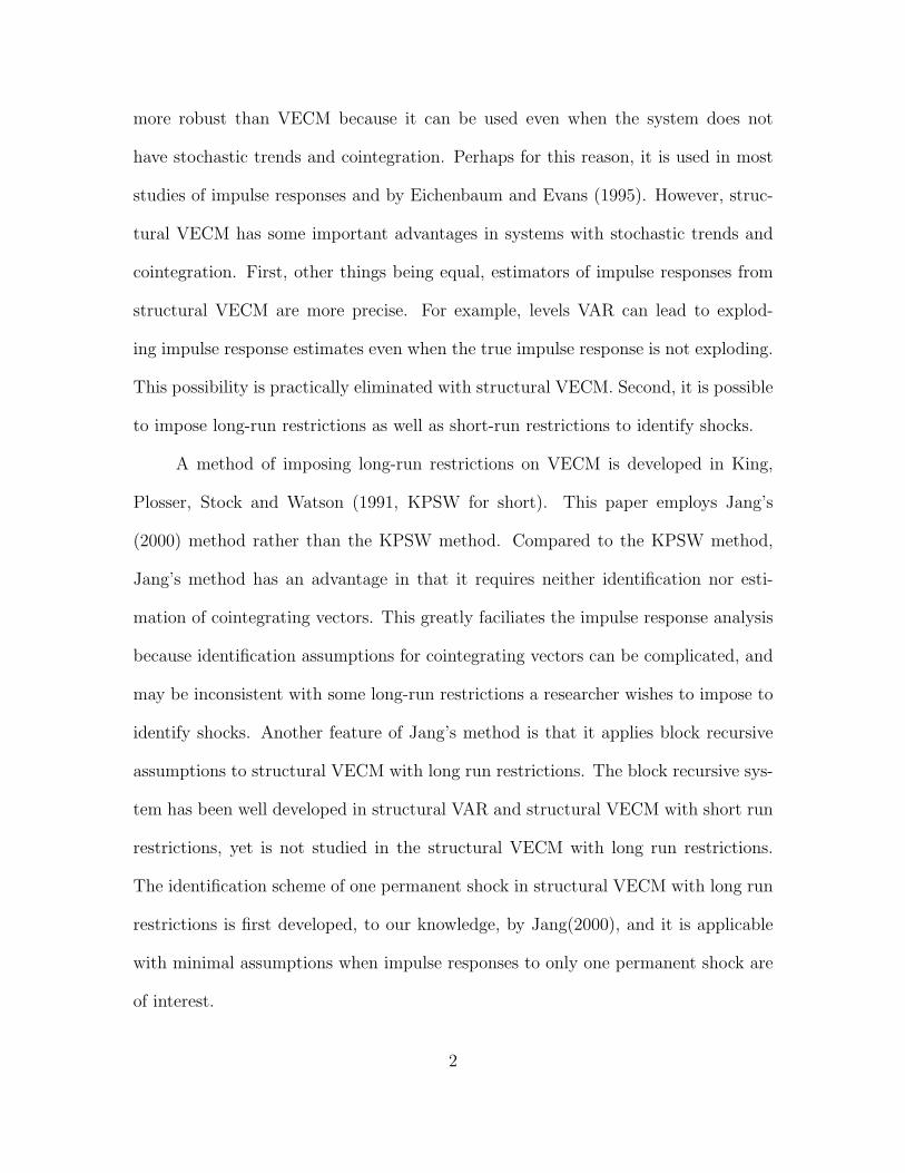
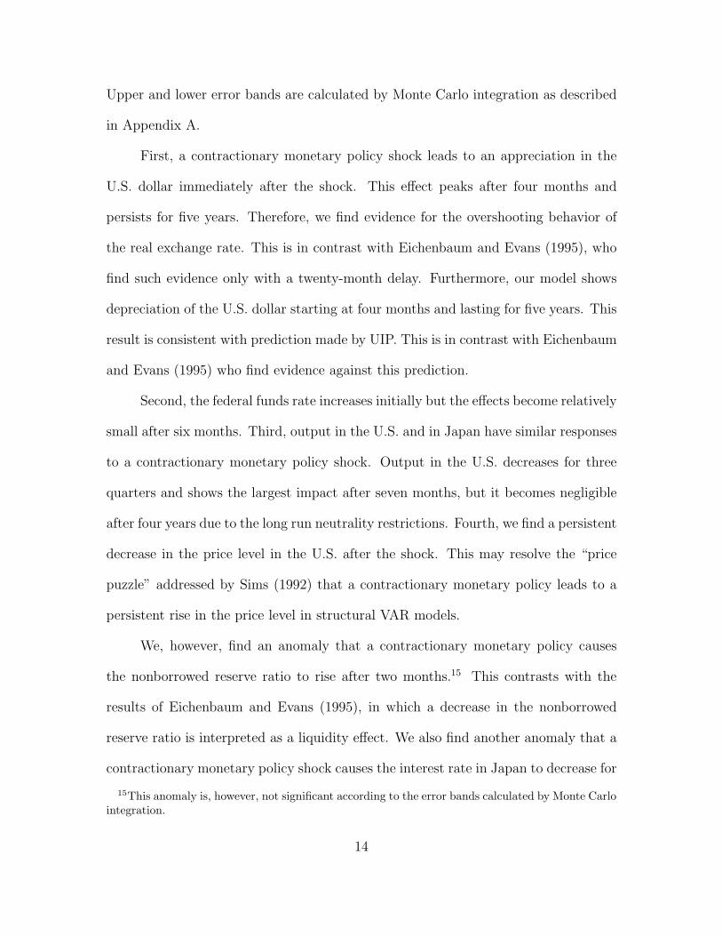
Figure 3.2: Impulse Responses to Contractionary Monetary Shockswith Long Run Restrictions on VECM
-0.06
-0.05
-0.04
-0.03
-0.02
-0.01
0
0 20 40 60 80 100 120
Res
pons
e
Month
Real Exchange Rates-0.6
-0.4
-0.2
0
0.2
0.4
0.6
0.8
1
1.2
1.4
0 20 40 60 80 100 120
Res
pons
e
Month
Federal Funds Rates in U.S.Interest Rates in Japan
-0.018
-0.016
-0.014
-0.012
-0.01
-0.008
-0.006
-0.004
-0.002
0
0.002
0 20 40 60 80 100 120
Res
pons
e
Month
Output in U.S.Output in Japan
-0.025
-0.02
-0.015
-0.01
-0.005
0
0 20 40 60 80 100 120
Res
pons
e
Month
Price in U.S.
Note: Contractionary monetary shocks are mesured by positive unit shock to the federal funds rates. VECM uses six variables: federalfunds rates, output in U.S., price in U.S., output in Japan, interest rates in Japan, and real exchange rate(dollar/yen). The lag lengthis five, which is equivalent to six in levels VAR in Eichenbaum and Evans(1995). Long run restrictions are imposed that monetaryshocks do not affect output in U.S., output in Japan, interest rates in Japan, and real exchange rates in the long run. Monetary shocksare normalized to have initial unit effects on federal funds rates.
substantial periods. Some of our results were sensitive to the choice of cointegration
rank. This often happens in models with long run restrictions as pointed out in Faust
and Leaper (1997).
3.2 A Six-variable VECM with Long Run Restrictions
As we find an anomaly of responses in the nonborrowed reserve ratio, we consider
a benchmark model with six variables dropping nonborrowed reserve ratio. We select
five lags and estimate the model assuming one cointegrating relation to impose the
same long run restrictions as the model in Section 3.1, which implies that there are
five permanent shocks in the structural VECM and four long run restrictions are
required to identify the monetary policy shock as in Section 3.1.
Figure 3.2 describes the impulse responses to a contractionary monetary policy
shock. Most results are similar to those of the seven-variable model in Section 3.1.
15
First, the U.S. dollar exhibits persistent appreciation for seven years compared to the
original value. Second, the federal funds rate rises in the initial period but the effects
become negative after seven months. Third, output in the U.S. shows persistent
negative effects but much longer than those of the previous model. Fourth, the price
level decreases after a contractionary monetary policy shock.
4 Impulse Response Analysis in VECM with Short Run Re-strictions
4.1 Block Recursive Assumptions in VECM
The reduced form VECM in (2.2) can be represented as a structural form:
B∗(L)∆xt = B0µ−B(1)xt−1 + vt (4.1)
where B∗(L) = B0−∑p−1
i=1 B∗i L
i, B∗(L) = B0A∗(L), B(1) = B0A(1), B∗i = B0A∗
i , and
vt = B0εt. The short run restrictions are imposed on B0 to have a block recursive
structure. See Christiano et al. (1999) and Keating (1999) for an extended theoretical
background. Partitioning xt into three blocks is convenient to illustrate the block
recursive structure:
xt =
x1t
st
x2t
, (4.2)
where xt is a vector of n(= n1 + 1 + n2) variables of interest, st is a monetary policy
variable, and x1t includes n1 variables which are in the information set when the
Fed implements a monetary policy while x2t contains n2 variables which are excluded
from the information set. Alternatively, x1t does not respond to a monetary policy
shock contemporaneously while x2t does. The block recursive assumption imposes
16
zero restrictions on the following partitioned B0:
B0 =
b11 0 0(n1 × n1) (n1 × 1) (n1 × n2)
b21 b22 0(1× n1) (1× 1) (1× n2)
b31 b32 b33
(n2 × n1) (n2 × 1) (n2 × n2)
(4.3)
Two zero restrictions, b12 = b13 = 0, are required for the monetary policy shock to
be orthogonal to other structural shocks, while the restriction, b23 = 0, implies the
assumption that the Fed does not have information about variables in x2t when it
makes a monetary policy decision.
The block recursive structure gives sufficient conditions to identify a monetary
policy shock, and the ordering within x1t and x2t does not affect the results if one is
interested in the effects of a monetary policy shock. Instead, the ordering across two
groups might affect the results substantially. This is a crucial issue in the structural
VECM as well as VAR models, while the ordering does not affect the results in the
VECM with long run restrictions.
We investigate impulse responses in the structural VECM changing the order
of variables and the measure of a monetary policy in the following sections.
4.2 Interpreting federal funds rate as a monetary policy
We begin with VECM when we measure federal funds rate as a monetary policy.
As discussed in Section 3.1, we estimate the model using two cointegrating vectors
with five lags for all the models in the following sections.
We follow the order in Eichenbaum and Evans (1995). Seven variables are
ordered by output in the U.S. (yus), the price level in the U.S. (Pus), output in Japan
(yjp), the interest rate in Japan (rjp), federal funds rates (rff ), the nonborrowed
17
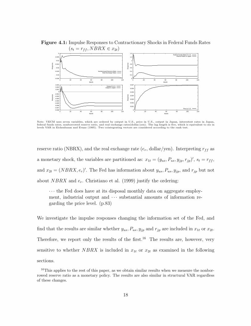
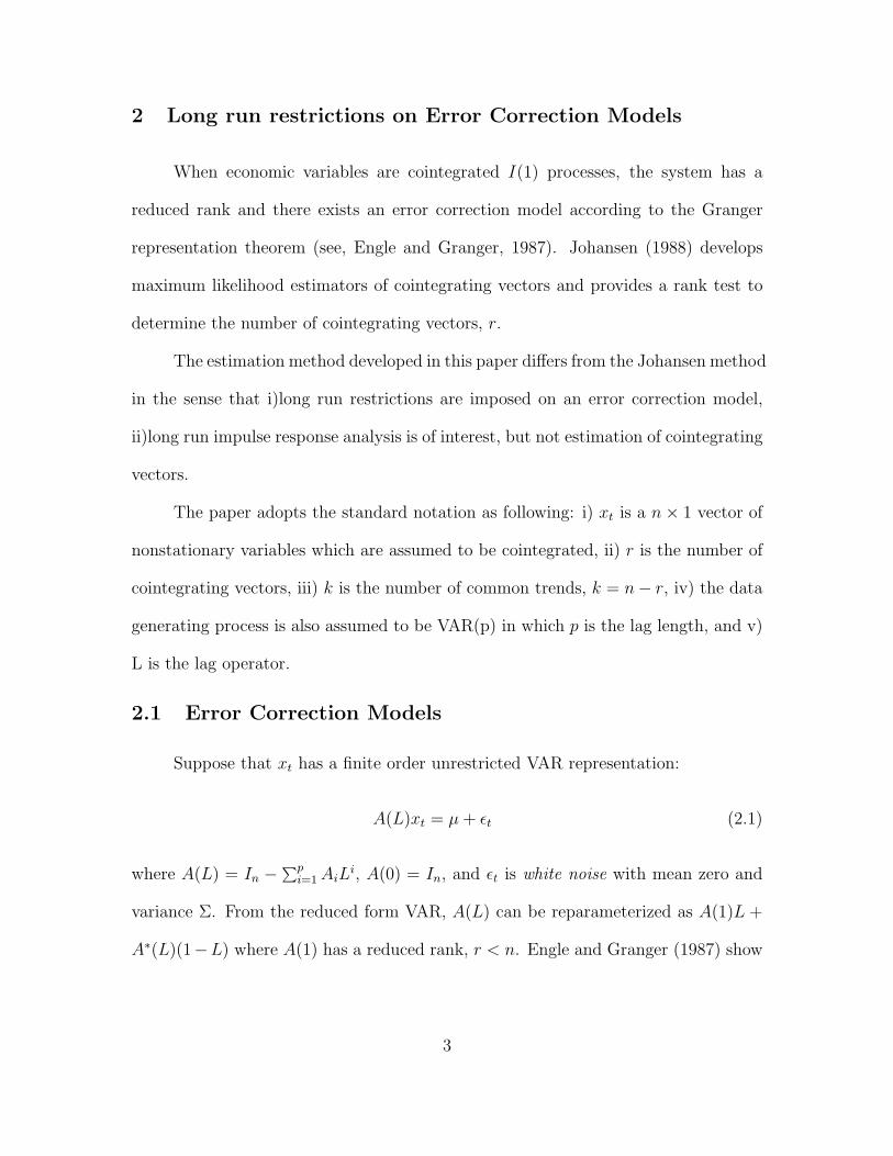
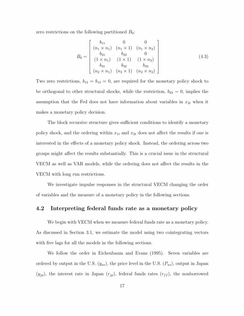
Figure 4.1: Impulse Responses to Contractionary Shocks in Federal Funds Rates(st = rff , NBRX ∈ x2t)
-0.035
-0.03
-0.025
-0.02
-0.015
-0.01
-0.005
0
0 20 40 60 80 100 120
Res
pons
e
Month
Nonborrowed Reserve RatioReal Exchange Rates
0
0.2
0.4
0.6
0.8
1
1.2
1.4
0 20 40 60 80 100 120
Res
pons
e
Month
Federal Funds Rates in U.S.Interest Rates in Japan
-0.008
-0.007
-0.006
-0.005
-0.004
-0.003
-0.002
-0.001
0
0.001
0.002
0.003
0 20 40 60 80 100 120
Res
pons
e
Month
Output in U.S.Output in Japan
0
0.001
0.002
0.003
0.004
0.005
0.006
0.007
0 20 40 60 80 100 120
Res
pons
e
Month
Price in U.S.
Note: VECM uses seven variables, which are ordered by output in U.S., price in U.S., output in Japan, interestest rates in Japan,federal funds rates, nonborrowed reserve ratio, and real exchange rates(dollar/yen). The lag length is five, which is equivalent to six inlevels VAR in Eichenbaum and Evans (1995). Two cointegrating vectors are considered according to the rank test.
reserve ratio (NBRX), and the real exchange rate (er, dollar/yen). Interpreting rff as
a monetary shock, the variables are partitioned as: x1t = (yus, Pus, yjp, rjp)′, st = rff ,
and x2t = (NBRX, er)′. The Fed has information about yus, Pus, yjp, and rjp but not
about NBRX and er. Christiano et al. (1999) justify the ordering:
· · · the Fed does have at its disposal monthly data on aggregate employ-ment, industrial output and · · · substantial amounts of information re-garding the price level. (p.83)
We investigate the impulse responses changing the information set of the Fed, and
find that the results are similar whether yus, Pus, yjp and rjp are included in x1t or x2t.
Therefore, we report only the results of the first.16 The results are, however, very
sensitive to whether NBRX is included in x1t or x2t as examined in the following
sections.
16This applies to the rest of this paper, as we obtain similar results when we measure the nonbor-rowed reserve ratio as a monetary policy. The results are also similar in structural VAR regardlessof these changes.
18
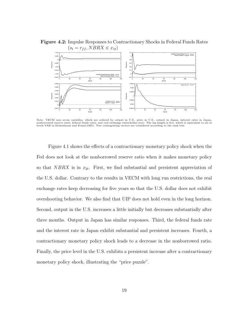
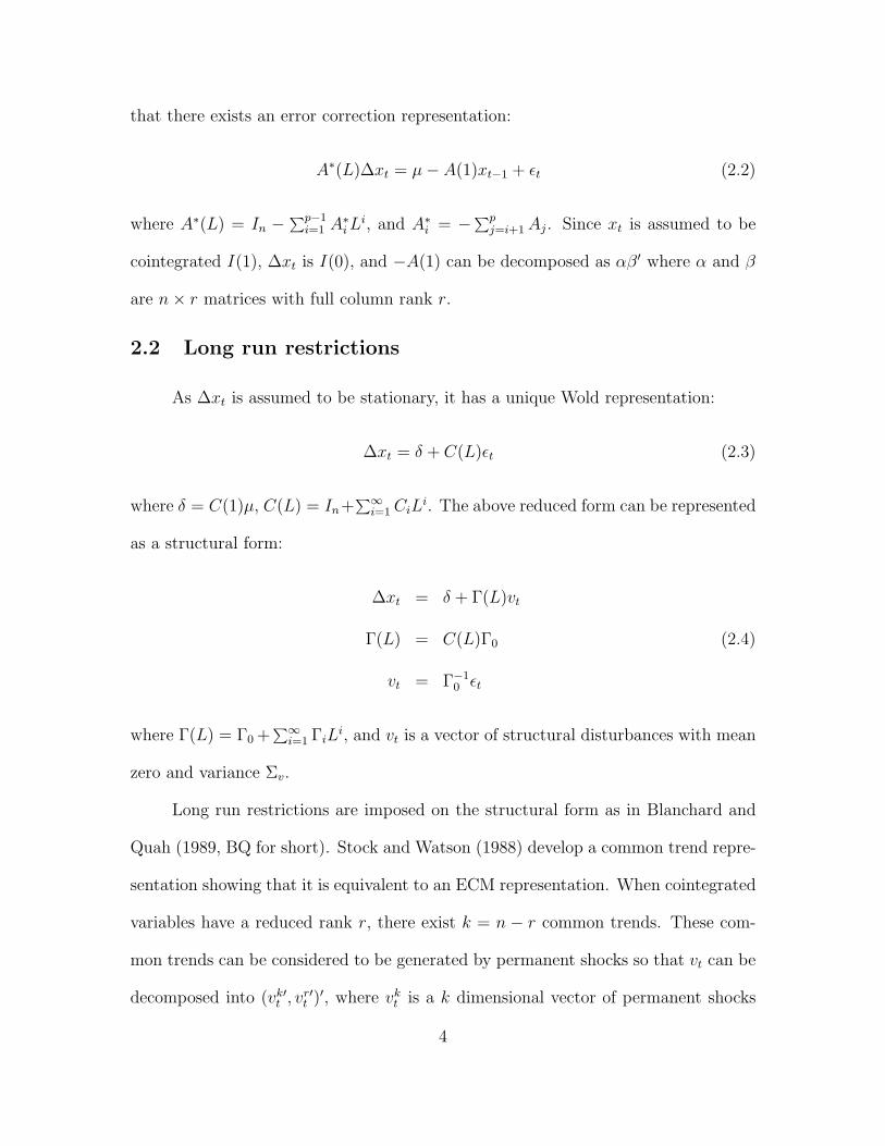
Figure 4.2: Impulse Responses to Contractionary Shocks in Federal Funds Rates(st = rff , NBRX ∈ x1t)
-0.025
-0.02
-0.015
-0.01
-0.005
0
0.005
0.01
0 20 40 60 80 100 120
Res
pons
e
Month
Nonborrowed Reserve RatioReal Exchange Rates
-0.2
0
0.2
0.4
0.6
0.8
1
1.2
0 20 40 60 80 100 120
Res
pons
e
Month
Federal Funds Rates in U.S.Interest Rates in Japan
-0.001
0
0.001
0.002
0.003
0.004
0.005
0.006
0 20 40 60 80 100 120
Res
pons
e
Month
Output in U.S.Output in Japan
-0.0015
-0.001
-0.0005
0
0.0005
0.001
0.0015
0 20 40 60 80 100 120
Res
pons
e
Month
Price in U.S.
Note: VECM uses seven variables, which are ordered by output in U.S., price in U.S., output in Japan, interest rates in Japan,nonborrowed reserve ratio, federal funds rates, and real exchange rates(dollar/yen). The lag length is five, which is equivalent to six inlevels VAR in Eichenbaum and Evans(1995). Two cointegrating vectors are considered according to the rank test.
Figure 4.1 shows the effects of a contractionary monetary policy shock when the
Fed does not look at the nonborrowed reserve ratio when it makes monetary policy
so that NBRX is in x2t. First, we find substantial and persistent appreciation of
the U.S. dollar. Contrary to the results in VECM with long run restrictions, the real
exchange rates keep decreasing for five years so that the U.S. dollar does not exhibit
overshooting behavior. We also find that UIP does not hold even in the long horizon.
Second, output in the U.S. increases a little initially but decreases substantially after
three months. Output in Japan has similar responses. Third, the federal funds rate
and the interest rate in Japan exhibit substantial and persistent increases. Fourth, a
contractionary monetary policy shock leads to a decrease in the nonborrowed ratio.
Finally, the price level in the U.S. exhibits a persistent increase after a contractionary
monetary policy shock, illustrating the “price puzzle”.
19
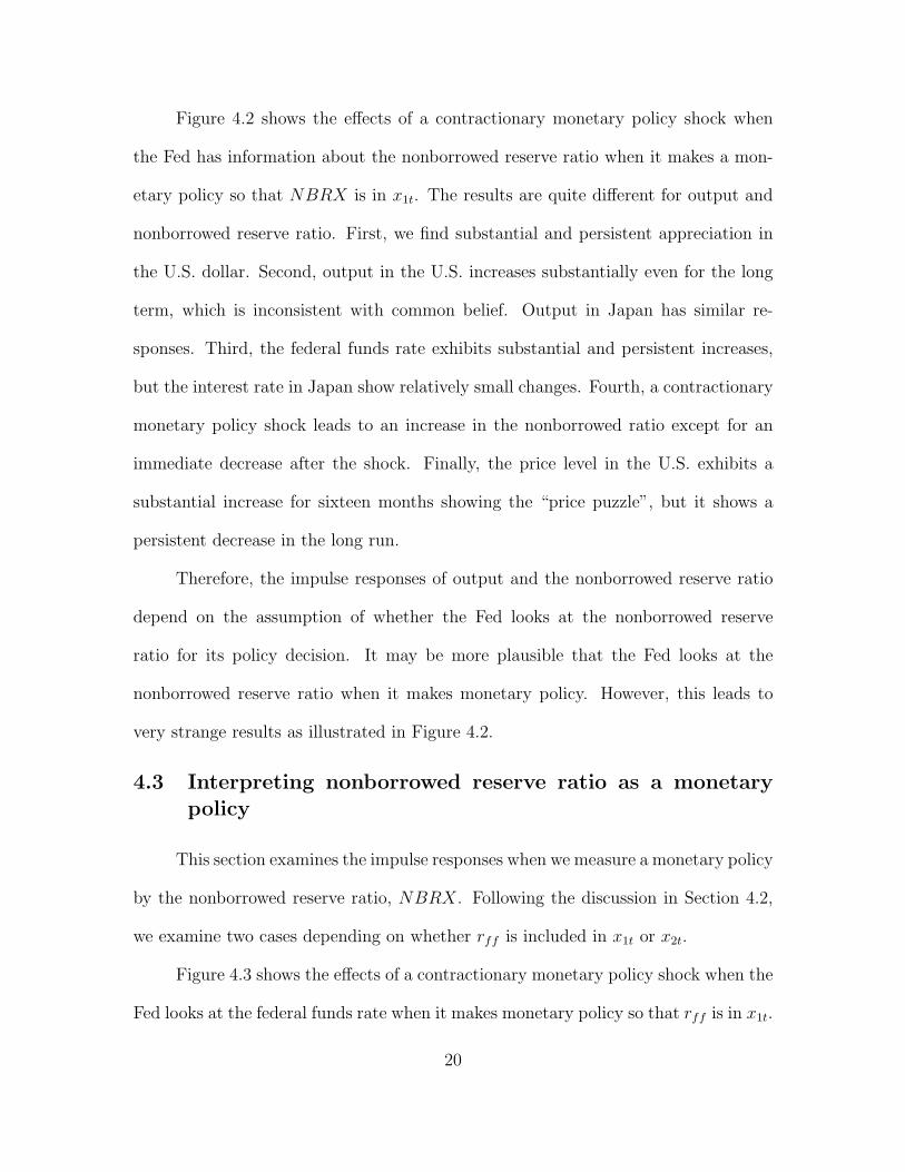
Figure 4.2 shows the effects of a contractionary monetary policy shock when
the Fed has information about the nonborrowed reserve ratio when it makes a mon-
etary policy so that NBRX is in x1t. The results are quite different for output and
nonborrowed reserve ratio. First, we find substantial and persistent appreciation in
the U.S. dollar. Second, output in the U.S. increases substantially even for the long
term, which is inconsistent with common belief. Output in Japan has similar re-
sponses. Third, the federal funds rate exhibits substantial and persistent increases,
but the interest rate in Japan show relatively small changes. Fourth, a contractionary
monetary policy shock leads to an increase in the nonborrowed ratio except for an
immediate decrease after the shock. Finally, the price level in the U.S. exhibits a
substantial increase for sixteen months showing the “price puzzle”, but it shows a
persistent decrease in the long run.
Therefore, the impulse responses of output and the nonborrowed reserve ratio
depend on the assumption of whether the Fed looks at the nonborrowed reserve
ratio for its policy decision. It may be more plausible that the Fed looks at the
nonborrowed reserve ratio when it makes monetary policy. However, this leads to
very strange results as illustrated in Figure 4.2.
4.3 Interpreting nonborrowed reserve ratio as a monetarypolicy
This section examines the impulse responses when we measure a monetary policy
by the nonborrowed reserve ratio, NBRX. Following the discussion in Section 4.2,
we examine two cases depending on whether rff is included in x1t or x2t.
Figure 4.3 shows the effects of a contractionary monetary policy shock when the
Fed looks at the federal funds rate when it makes monetary policy so that rff is in x1t.
20
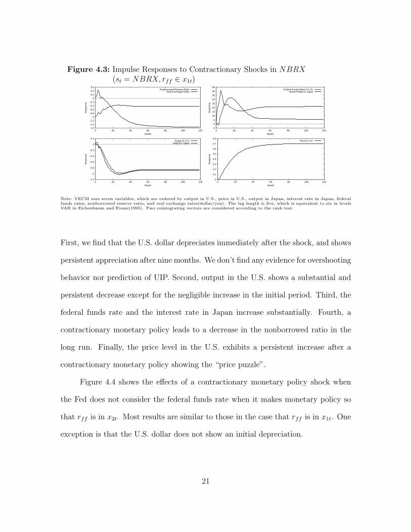
Figure 4.3: Impulse Responses to Contractionary Shocks in NBRX(st = NBRX, rff ∈ x1t)
-1.6
-1.4
-1.2
-1
-0.8
-0.6
-0.4
-0.2
0
0.2
0.4
0.6
0 20 40 60 80 100 120
Res
pons
e
Month
Nonborrowed Reserve RatioReal Exchange Rates
-5
0
5
10
15
20
25
30
35
40
45
0 20 40 60 80 100 120
Res
pons
e
Month
Federal Funds Rates in U.S.Interest Rates in Japan
-1.2
-1
-0.8
-0.6
-0.4
-0.2
0
0.2
0 20 40 60 80 100 120
Res
pons
e
Month
Output in U.S.Output in Japan
0
0.1
0.2
0.3
0.4
0.5
0.6
0.7
0.8
0 20 40 60 80 100 120
Res
pons
e
Month
Price in U.S.
Note: VECM uses seven variables, which are ordered by output in U.S., price in U.S., output in Japan, interest rate in Japan, federalfunds rates, nonborrowed reserve ratio, and real exchange rates(dollar/yen). The lag length is five, which is equivalent to six in levelsVAR in Eichenbaum and Evans(1995). Two cointegrating vectors are considered according to the rank test.
First, we find that the U.S. dollar depreciates immediately after the shock, and shows
persistent appreciation after nine months. We don’t find any evidence for overshooting
behavior nor prediction of UIP. Second, output in the U.S. shows a substantial and
persistent decrease except for the negligible increase in the initial period. Third, the
federal funds rate and the interest rate in Japan increase substantially. Fourth, a
contractionary monetary policy leads to a decrease in the nonborrowed ratio in the
long run. Finally, the price level in the U.S. exhibits a persistent increase after a
contractionary monetary policy showing the “price puzzle”.
Figure 4.4 shows the effects of a contractionary monetary policy shock when
the Fed does not consider the federal funds rate when it makes monetary policy so
that rff is in x2t. Most results are similar to those in the case that rff is in x1t. One
exception is that the U.S. dollar does not show an initial depreciation.
21
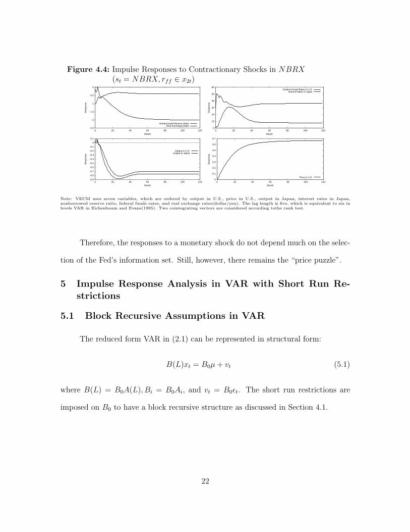
Figure 4.4: Impulse Responses to Contractionary Shocks in NBRX(st = NBRX, rff ∈ x2t)
-2.5
-2
-1.5
-1
-0.5
0
0 20 40 60 80 100 120
Res
pons
e
Month
Nonborrowed Reserve RatioReal Exchange Rates
0
10
20
30
40
50
60
0 20 40 60 80 100 120
Res
pons
e
Month
Federal Funds Rates in U.S.Interest Rates in Japan
-0.9
-0.8
-0.7
-0.6
-0.5
-0.4
-0.3
-0.2
-0.1
0
0.1
0 20 40 60 80 100 120
Res
pons
e
Month
Output in U.S.Output in Japan
0
0.1
0.2
0.3
0.4
0.5
0.6
0.7
0 20 40 60 80 100 120
Res
pons
e
Month
Price in U.S.
Note: VECM uses seven variables, which are ordered by output in U.S., price in U.S., output in Japan, interest rates in Japan,nonborrowed reserve ratio, federal funds rates, and real exchange rates(dollar/yen). The lag length is five, which is equivalent to six inlevels VAR in Eichenbaum and Evans(1995). Two cointegrating vectors are considered according tothe rank test.
Therefore, the responses to a monetary shock do not depend much on the selec-
tion of the Fed’s information set. Still, however, there remains the “price puzzle”.
5 Impulse Response Analysis in VAR with Short Run Re-strictions
5.1 Block Recursive Assumptions in VAR
The reduced form VAR in (2.1) can be represented in structural form:
B(L)xt = B0µ + vt (5.1)
where B(L) = B0A(L), Bi = B0Ai, and vt = B0εt. The short run restrictions are
imposed on B0 to have a block recursive structure as discussed in Section 4.1.
22
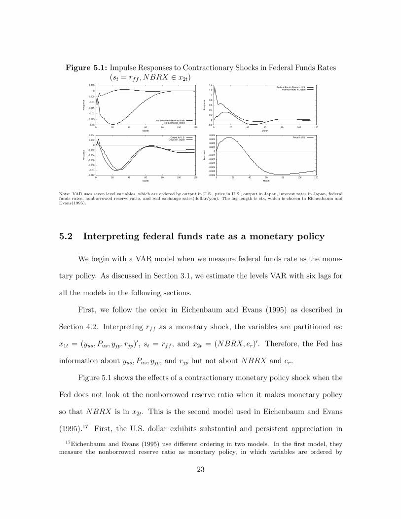
Figure 5.1: Impulse Responses to Contractionary Shocks in Federal Funds Rates(st = rff , NBRX ∈ x2t)
-0.03
-0.025
-0.02
-0.015
-0.01
-0.005
0
0.005
0 20 40 60 80 100 120
Res
pons
e
Month
Nonborrowed Reserve RatioReal Exchange Rates
-0.2
0
0.2
0.4
0.6
0.8
1
1.2
1.4
0 20 40 60 80 100 120
Res
pons
e
Month
Federal Funds Rates in U.S.Interest Rates in Japan
-0.012
-0.01
-0.008
-0.006
-0.004
-0.002
0
0.002
0.004
0 20 40 60 80 100 120
Res
pons
e
Month
Output in U.S.Output in Japan
-0.006
-0.005
-0.004
-0.003
-0.002
-0.001
0
0.001
0.002
0.003
0.004
0 20 40 60 80 100 120
Res
pons
e
Month
Price in U.S.
Note: VAR uses seven level variables, which are ordered by output in U.S., price in U.S., output in Japan, interest rates in Japan, federalfunds rates, nonborrowed reserve ratio, and real exchange rates(dollar/yen). The lag length is six, which is chosen in Eichenbaum andEvans(1995).
5.2 Interpreting federal funds rate as a monetary policy
We begin with a VAR model when we measure federal funds rate as the mone-
tary policy. As discussed in Section 3.1, we estimate the levels VAR with six lags for
all the models in the following sections.
First, we follow the order in Eichenbaum and Evans (1995) as described in
Section 4.2. Interpreting rff as a monetary shock, the variables are partitioned as:
x1t = (yus, Pus, yjp, rjp)′, st = rff , and x2t = (NBRX, er)′. Therefore, the Fed has
information about yus, Pus, yjp, and rjp but not about NBRX and er.
Figure 5.1 shows the effects of a contractionary monetary policy shock when the
Fed does not look at the nonborrowed reserve ratio when it makes monetary policy
so that NBRX is in x2t. This is the second model used in Eichenbaum and Evans
(1995).17 First, the U.S. dollar exhibits substantial and persistent appreciation in
17Eichenbaum and Evans (1995) use different ordering in two models. In the first model, theymeasure the nonborrowed reserve ratio as monetary policy, in which variables are ordered by
23
real value. In contrast to the results in VECM with long run restrictions, the real
exchange rate keeps decreasing for twenty months and exhibits delayed overshooting
behavior. There is no evidence of the UIP prediction, as the exchange rate does
not bounce back for the initial twenty months. Second, output in the U.S. increases
somewhat initially but decreases substantially after three months. Output in the
U.S., however, returns to the original level after five years, and decreases a little after
then. Output in Japan has similar responses. Third, the federal funds rate rises in
the initial period but returns to its original level after three years. The interest rate
in Japan also shows a rise in levels for three years. Fourth, a contractionary monetary
policy shock leads to a decrease in the nonborrowed ratio, but it returns to the initial
level after twenty months. Finally, the price level in the U.S. exhibits a substantial
increase for three years showing the “price puzzle”, but decreases in the long run.
Figure 5.2 shows the effects of a contractionary monetary policy shock when the
Fed has information about the nonborrowed reserve ratio when it makes monetary
policy so that NBRX is in x1t. The results are similar to those in Figure 5.1 except
that the nonborrowed reserve ratio shows a small increase in the initial five months.
yus, Pus, yjp, rjp, NBRX, rff , and er. From the block recursive assumption, the Fed does not lookat current level of the federal funds rate when it makes monetary policy decision or, alternatively,the federal funds rate responds to monetary policy contemporaneously. See Figure II, p.990. In thesecond model, they choose the federal funds rate as a monetary policy measure, in which variablesare ordered by yus, Pus, yjp, rjp, rff , NBRX, and er. The corresponding assumption is that the Feddoes not look at current value of the nonborrowed reserve ratio or, alternatively, the nonborrowedreserve ratio responds to monetary policy contemporaneously. See Figure III, p.995.
24
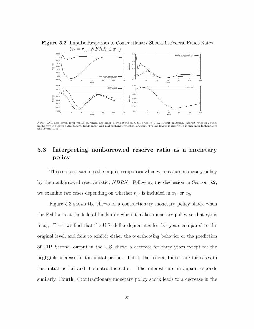
Figure 5.2: Impulse Responses to Contractionary Shocks in Federal Funds Rates(st = rff , NBRX ∈ x1t)
-0.035
-0.03
-0.025
-0.02
-0.015
-0.01
-0.005
0
0.005
0 20 40 60 80 100 120
Res
pons
e
Month
Nonborrowed Reserve RatioReal Exchange Rates
-0.2
0
0.2
0.4
0.6
0.8
1
1.2
0 20 40 60 80 100 120
Res
pons
e
Month
Federal Funds Rates in U.S.Interest Rates in Japan
-0.01
-0.008
-0.006
-0.004
-0.002
0
0.002
0.004
0 20 40 60 80 100 120
Res
pons
e
Month
Output in U.S.Output in Japan
-0.01
-0.008
-0.006
-0.004
-0.002
0
0.002
0 20 40 60 80 100 120
Res
pons
e
Month
Price in U.S.
Note: VAR uses seven level variables, which are ordered by output in U.S., price in U.S., output in Japan, interest rates in Japan,nonborrowed reserve ratio, federal funds rates, and real exchange rates(dollar/yen). The lag length is six, which is chosen in Eichenbaumand Evans(1995).
5.3 Interpreting nonborrowed reserve ratio as a monetarypolicy
This section examines the impulse responses when we measure monetary policy
by the nonborrowed reserve ratio, NBRX. Following the discussion in Section 5.2,
we examine two cases depending on whether rff is included in x1t or x2t.
Figure 5.3 shows the effects of a contractionary monetary policy shock when
the Fed looks at the federal funds rate when it makes monetary policy so that rff is
in x1t. First, we find that the U.S. dollar depreciates for five years compared to the
original level, and fails to exhibit either the overshooting behavior or the prediction
of UIP. Second, output in the U.S. shows a decrease for three years except for the
negligible increase in the initial period. Third, the federal funds rate increases in
the initial period and fluctuates thereafter. The interest rate in Japan responds
similarly. Fourth, a contractionary monetary policy shock leads to a decrease in the
25
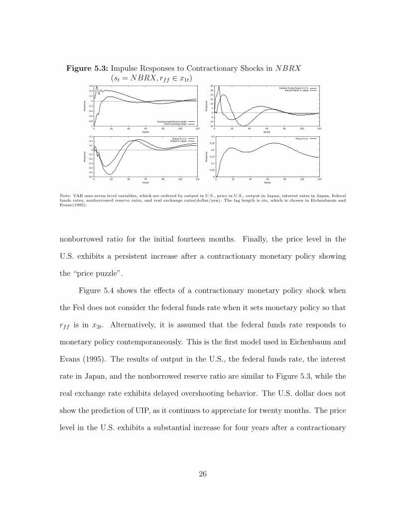
Figure 5.3: Impulse Responses to Contractionary Shocks in NBRX(st = NBRX, rff ∈ x1t)
-1
-0.8
-0.6
-0.4
-0.2
0
0.2
0.4
0.6
0 20 40 60 80 100 120
Res
pons
e
Month
Nonborrowed Reserve RatioReal Exchange Rates
-15
-10
-5
0
5
10
15
20
25
30
0 20 40 60 80 100 120
Res
pons
e
Month
Federal Funds Rates in U.S.Interest Rates in Japan
-0.6
-0.5
-0.4
-0.3
-0.2
-0.1
0
0.1
0.2
0.3
0 20 40 60 80 100 120
Res
pons
e
Month
Output in U.S.Output in Japan
0
0.05
0.1
0.15
0.2
0.25
0.3
0 20 40 60 80 100 120
Res
pons
e
Month
Price in U.S.
Note: VAR uses seven level variables, which are ordered by output in U.S., price in U.S., output in Japan, interest rates in Japan, federalfunds rates, nonborrowed reserve ratio, and real exchange rates(dollar/yen). The lag length is six, which is chosen in Eichenbaum andEvans(1995).
nonborrowed ratio for the initial fourteen months. Finally, the price level in the
U.S. exhibits a persistent increase after a contractionary monetary policy showing
the “price puzzle”.
Figure 5.4 shows the effects of a contractionary monetary policy shock when
the Fed does not consider the federal funds rate when it sets monetary policy so that
rff is in x2t. Alternatively, it is assumed that the federal funds rate responds to
monetary policy contemporaneously. This is the first model used in Eichenbaum and
Evans (1995). The results of output in the U.S., the federal funds rate, the interest
rate in Japan, and the nonborrowed reserve ratio are similar to Figure 5.3, while the
real exchange rate exhibits delayed overshooting behavior. The U.S. dollar does not
show the prediction of UIP, as it continues to appreciate for twenty months. The price
level in the U.S. exhibits a substantial increase for four years after a contractionary
26
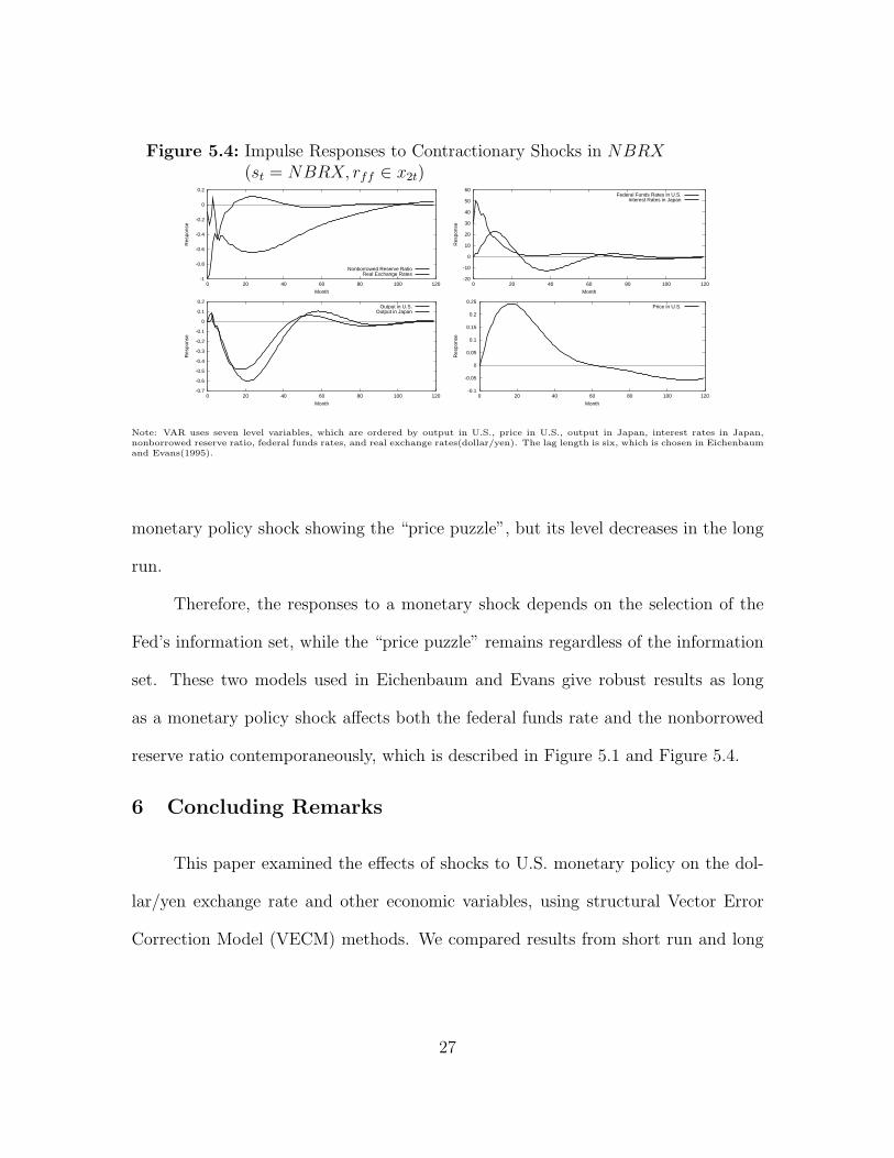
Figure 5.4: Impulse Responses to Contractionary Shocks in NBRX(st = NBRX, rff ∈ x2t)
-1
-0.8
-0.6
-0.4
-0.2
0
0.2
0 20 40 60 80 100 120
Res
pons
e
Month
Nonborrowed Reserve RatioReal Exchange Rates
-20
-10
0
10
20
30
40
50
60
0 20 40 60 80 100 120
Res
pons
e
Month
Federal Funds Rates in U.S.Interest Rates in Japan
-0.7
-0.6
-0.5
-0.4
-0.3
-0.2
-0.1
0
0.1
0.2
0 20 40 60 80 100 120
Res
pons
e
Month
Output in U.S.Output in Japan
-0.1
-0.05
0
0.05
0.1
0.15
0.2
0.25
0 20 40 60 80 100 120
Res
pons
e
Month
Price in U.S.
Note: VAR uses seven level variables, which are ordered by output in U.S., price in U.S., output in Japan, interest rates in Japan,nonborrowed reserve ratio, federal funds rates, and real exchange rates(dollar/yen). The lag length is six, which is chosen in Eichenbaumand Evans(1995).
monetary policy shock showing the “price puzzle”, but its level decreases in the long
run.
Therefore, the responses to a monetary shock depends on the selection of the
Fed’s information set, while the “price puzzle” remains regardless of the information
set. These two models used in Eichenbaum and Evans give robust results as long
as a monetary policy shock affects both the federal funds rate and the nonborrowed
reserve ratio contemporaneously, which is described in Figure 5.1 and Figure 5.4.
6 Concluding Remarks
This paper examined the effects of shocks to U.S. monetary policy on the dol-
lar/yen exchange rate and other economic variables, using structural Vector Error
Correction Model (VECM) methods. We compared results from short run and long
27
run restrictions imposed on the structural VECM, and compared our estimates of the
impulse responses with those based on levels Vector Autoregression.
From the empirical studies in this paper, we found that estimates of the impulse
responses are sensitive to the choice of restrictions. We found evidence for immedi-
ate appreciation followed by gradual depreciation in the U.S. dollar with long run
restrictions in VECM, but failed to find such evidence with short run restrictions in
VECM or in levels VAR. We also resolve the “price puzzle” in VECM with long run
restrictions, which is often found in levels VAR.
28
REFERENCES
Christiano, L. J., M. Eichenbaum, and C. L. Evans (1999): “Monetary PolicyShocks: What Have We Learned and to What End?”, in Handbook of Macroeco-nomics, ed. by J. Tayor, and M. Woodford, vol. 1, chap. 2, pp. 65–148. ElsevierScience.
Doan, T. A. (1992): RATS User’s Manual, Version 4. Estima, Evanston, IL.
Dornbusch, R. (1976): “Expectations and Exchange Rate Dynamics”, JournalPolitical Economy, 84(6), 1161–76.
Eichenbaum, M., and C. L. Evans (1995): “Some Empirical Evidence on theEffects of Shocks to Monetary Policy on Exchange Rates”, Quarterly Journal ofEconomics, 110, 975–1009.
Engle, R. F., and C. Granger (1987): “Co-Integration and Error Correction:Representation, Estimation and Testing”, Econometrica, 55(2), 251–76.
Faust, J., and E. M. Leeper (1997): “When Do Long-Run Identifying RestrictionsGive Reliable Results?”, Journal of Business and Economic Statistics, 15(3), 345–53.
Fisher, L. A., P. L. Fackler, and D. Orden (1995): “Long-run IdentifyingRestrictions for an Error-Correction Model of New Zealand Mondy, Prices andOutput”, Journal of International Money and Finance, 14(1), 127–47.
Jang, K. (2000): “Impulse Response Analysis with Long Run Restrictions on ErrorCorrection Models”, Mimeo., Ohio State University.
Johansen, S. (1988): “Statistical Analysis of Cointegration Vectors”, Journal ofEconomic Dynamics and Control, 12, 231–54.
(1995): Likelihood-Based Inference in Cointegrated Vector AutoregressiveModels. Oxford University Press.
29
Keating, J. W. (1999): “Structural Inference With Long-Run Recursive Empir-ical Models”, Working Paper No. 1999-3, University of Kansas, forthcoming inMacroeconomic Dynamics.
Kilian, L. (1998b): “Small-Sample Confidence Intervals for Impulse Response Func-tions”, Review of Economics and Statistics, 80(2), 218–30.
King, R. G., C. I. Plosser, J. H. Stock, and M. W. Watson (1991): “Stochas-tic Trends and Economic Fluctuations”, American Economic Review, 81(4), 810–40.
Lutkepohl, H. (1990): “Asymptotic Distributions of Impulse Response Functionsand Forecast Error Variance Decompositions of Vector Autoregresssive Models”,Review of Economics and Statistics, 72(1), 116–25.
Lutkepohl, H., and H.-E. Reimers (1992): “Impulse response analysis of coin-tegrated systems”, Journal of Economic Dynamics and Control, 16, 53–78.
Ogaki, M., and J. Y. Park (1997): “A Cointegration Approach to EstimatingPreference Parameters”, Journal of Econometrics, 82, 107–34.
Runkle, D. E. (1987): “Vector Autoregression and Reality”, Journal of Businessand Economic Statistics, 5, 437–42.
Sims, C. A. (1980): “Macroeconomics and Reality”, Econometrica, 48, 1–48.
(1992): “Interpreting the Macroeconomic Time Series Facts: The Effects ofMonetary Policy”, European Economic Review, 36, 975–1000.
Sims, C. A., and T. Zha (1995): “Error Bands for Impulse Responses”, WorkingPaper Series 95-6, Federal Reserve Bank of Atlanta.
Stock, J. H., and M. W. Watson (1988): “Testing for Common Trends”, Journalof the American Statistical Association, 83(404), 1097–1107.
Zellner, A. (1971): An Introduction to Bayesian Inference in Econometrics. Wiley,New York.
30
APPENDIX A
Monte Carlo Integration
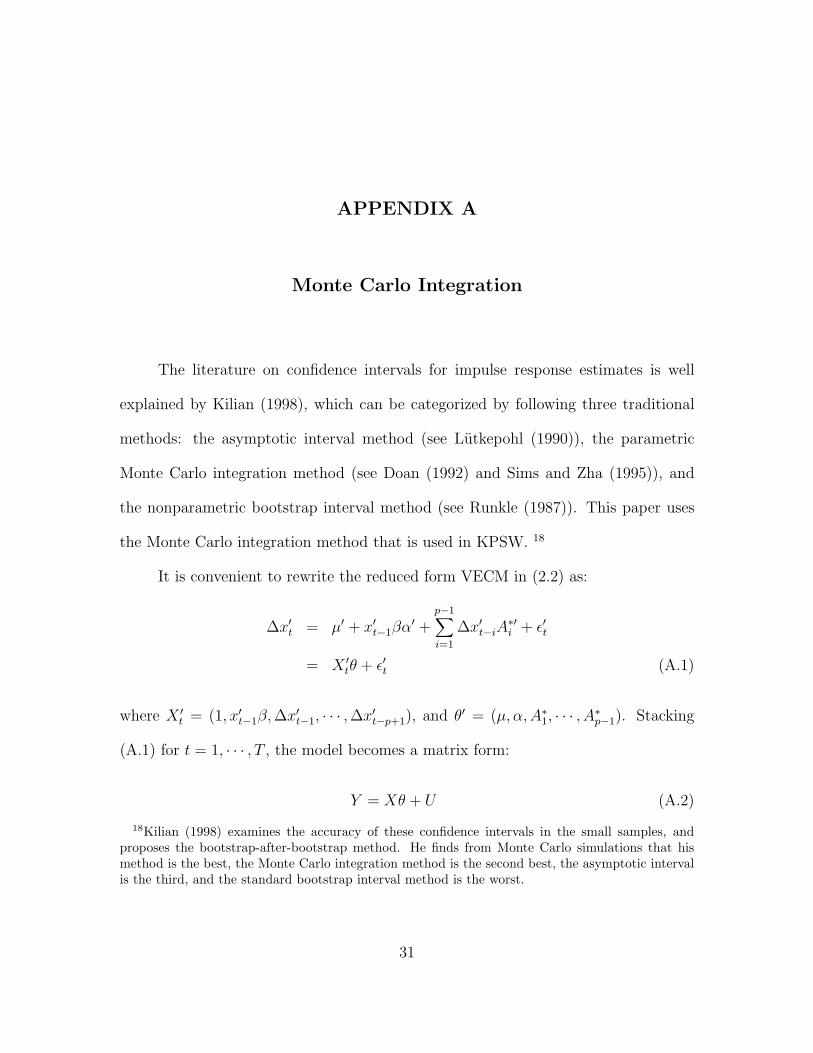
The literature on confidence intervals for impulse response estimates is well
explained by Kilian (1998), which can be categorized by following three traditional
methods: the asymptotic interval method (see Lutkepohl (1990)), the parametric
Monte Carlo integration method (see Doan (1992) and Sims and Zha (1995)), and
the nonparametric bootstrap interval method (see Runkle (1987)). This paper uses
the Monte Carlo integration method that is used in KPSW. 18
It is convenient to rewrite the reduced form VECM in (2.2) as:
∆x′t = µ′ + x′t−1βα′ +p−1∑
i=1∆x′t−iA
∗′i + ε′t
= X ′tθ + ε′t (A.1)
where X ′t = (1, x′t−1β, ∆x′t−1, · · · , ∆x′t−p+1), and θ′ = (µ, α,A∗
1, · · · , A∗p−1). Stacking
(A.1) for t = 1, · · · , T , the model becomes a matrix form:
Y = Xθ + U (A.2)
18Kilian (1998) examines the accuracy of these confidence intervals in the small samples, andproposes the bootstrap-after-bootstrap method. He finds from Monte Carlo simulations that hismethod is the best, the Monte Carlo integration method is the second best, the asymptotic intervalis the third, and the standard bootstrap interval method is the worst.
31
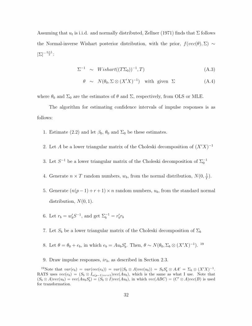
Assuming that ut is i.i.d. and normally distributed, Zellner (1971) finds that Σ follows
the Normal-inverse Wishart posterior distribution, with the prior, f(vec(θ), Σ) ∼
|Σ|−n+12 :
Σ−1 ∼ Wishart((TΣ0))−1, T ) (A.3)
θ ∼ N(θ0, Σ⊗ (X ′X)−1) with given Σ (A.4)
where θ0 and Σ0 are the estimates of θ and Σ, respectively, from OLS or MLE.
The algorithm for estimating confidence intervals of impulse responses is as
follows:
1. Estimate (2.2) and let β0, θ0 and Σ0 be these estimates.
2. Let A be a lower triangular matrix of the Choleski decomposition of (X ′X)−1
3. Let S−1 be a lower triangular matrix of the Choleski decomposition of Σ−10
4. Generate n× T random numbers, wb, from the normal distribution, N(0, 1T ).
5. Generate (n(p− 1)+ r +1)×n random numbers, ub, from the standard normal
distribution, N(0, 1).
6. Let rb = w′bS
−1, and get Σ−1b = r′brb
7. Let Sb be a lower triangular matrix of the Choleski decomposition of Σb
8. Let θ = θ0 + eb, in which eb = AubS′b. Then, θ ∼ N(θ0, Σb ⊗ (X ′X)−1). 19
9. Draw impulse responses, irb, as described in Section 2.3.
19Note that var(eb) = var(vec(eb)) = var((Sb ⊗ A)vec(ub)) = SbS′b ⊗ AA′ = Σb ⊗ (X ′X)−1.RATS uses vec(eb) = (Sb ⊗ In(p−1)+r+1)vec(Aub), which is the same as what I use. Note that(Sb ⊗ A)vec(ub) = vec(AubS′b) = (Sb ⊗ I)vec(Aub), in which vec(ABC) = (C ′ ⊗ A)vec(B) is usedfor transformation.
32
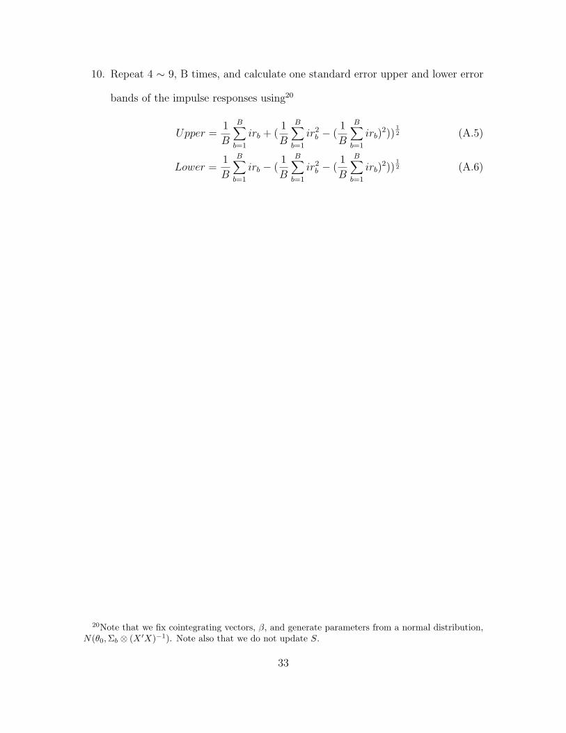
10. Repeat 4 ∼ 9, B times, and calculate one standard error upper and lower error
bands of the impulse responses using20
Upper =1B
B∑
b=1
irb + (1B
B∑
b=1
ir2b − (
1B
B∑
b=1
irb)2))12 (A.5)
Lower =1B
B∑
b=1
irb − (1B
B∑
b=1
ir2b − (
1B
B∑
b=1
irb)2))12 (A.6)
20Note that we fix cointegrating vectors, β, and generate parameters from a normal distribution,N(θ0, Σb ⊗ (X ′X)−1). Note also that we do not update S.
33