The Effects of Budget Deficits on Selected Macroeconomic

P a g e | 1

NKALU, Chigozie Nelson PG/MSc/14/69634

THE EFFECTS OF BUDGET DEFICITS ON SELECTED MACROECONOMIC VARIABLES IN

NIGERIA AND GHANA

DEPARTMENT OF ECONOMICS

FACULTY OF THE SOCIAL SCIENCES

Ebere Omeje Digitally Signed by: Content manager’s Name DN : CN = Webmaster’s name O= University of Nigeria, Nsukka OU = Innovation Centre

P a g e | 2

THE EFFECTS OF BUDGET DEFICITS ON SELECTED MACROECONOMIC

VARIABLES IN NIGERIA AND GHANA

By

NKALU, Chigozie Nelson

PG/MSc/14/69634



UNIVERSITY OF NIGERIA, NSUKKA

SEPTEMBER, 2015

P a g e | 3

THE EFFECTS OF BUDGET DEFICITS ON SELECTED MACROECONOMIC

VARIABLES IN NIGERIA AND GHANA

AnMSc. Thesis

By

NKALU, Chigozie Nelson

PG/MSc/14/69634



UNIVERSITY OF NIGERIA, NSUKKA

SUPERVISOR: PROF. C. C. AGU

SEPTEMBER, 2015

P a g e | 4

TITLE PAGE

The Effects of Budget Deficits on Selected Macroeconomic Variables in

Nigeria and Ghana

P a g e | 5

CERTIFICATION

This is to certify that NKALU, Chigozie Nelson, a post-graduate student of the Department

of Economics, University of Nigeria, Nsukka with Registration Number: PG/MSc/14/69634

has satisfactorily completed the requirements for the award of Master of Science (MSc.) in

Economics

____________________________ ____________________

Nkalu, Chigozie Nelson Date

PG/MSc/14/69634

(The Researcher)

________________ ___________________

Prof. C. C. Agu Date

(Supervisor)

________________ ___________________

Prof. S. I. Madueme Date

(Head of Department)

P a g e | 6

APPROVAL PAGE

This research work titled: “The Effects of Budget Deficits on Selected Macroeconomic

Variables in Nigeria and Ghana” has followed due process and has been approved to have

met the minimum requirement for the award of the Master of Science degree in the

Department of Economics, Faculty of the Social Sciences, University of Nigeria, Nsukka.

________________ ___________________

Prof. C. C. Agu Date

(Supervisor)

________________ ___________________

Prof. S. I. Madueme Date

(Head of Department, Economics)

________________ ____________________

Prof. A. I. Madu Date

(Dean, Faculty of the Social Sciences)

________________ ____________________

Date

(External Examiner)

P a g e | 7

DEDICATION

To:

My beloved mother

P a g e | 8

ACKNOWLEDGMENT

This study would not have been a huge success without the inputs of some men of goodwill.

Let me first and foremost express my deep gratitude to my family for whom I derive

unquenchable zeal to surmount some constraints in the course of this study. Special thanks to

my mother, brothers and sisters for the much love and encouragements which indeed has

reshaped my entire being. My most and sincere thanksgiving goes to the Almighty God for

His infinite mercies throughout my existence.

I must as a matter of fact recognize my able and capable supervisor and academic adviser –

Prof. C. C. Agu for his ever and relentless guidance and mentorship. My heartfelt gratitude

goes to my brothers, lecturers and senior colleagues in the Department of Economics,

University of Nigeria, Nsukka for their immeasurable contributions towards making this

study a colossal success. Special thanks to Dr. Jude O. Chukwu, Dr. Richard K. Edeme, Dr,

Emmanuel Nwosu, Dr. Ezebuilo R. Ukwueze, Dr. I. Ifelunini, Dr. (Mrs) Gladys Aneke, Prof.

(Mrs) S. I. Madueme, Miss Anaduaka Uchechi S., Emecheta Chisom, Nnetu Vivian, Mr.

Ekene and Mr. Nchege Johnson. Regrettably enough, others whose names cannot contain on

this page due to time and space constraints should bear with me.

Thank you all, and may our good Lord shower you with abundant blessings - Amen!

P a g e | 9

TABLE OF CONTENTS

Title Page - - - - - - - - - - i Certification - - - - - - - - - - ii Approval Page - - - - - - - - - iii Dedication - - - - - - - - - - iv Acknowledgement - - - - - - - - - v Table of Contents - - - - - - - - - vi List of Figures - - - - - - - - - ix List of Tables - - - - - - - - - - x Abstract - - - - - - - - - - xi CHAPTER ONE: INTRODUCTION

1.1 Background of the Study - - - - - - - 1

1.2 Statement of the Problem - - - - - - - 4

1.3 Research Questions - - - - - - - 7

1.4 Objectives of the Study - - - - - - - 8

1.5 Hypotheses of the Study - - - - - - - 8

1.6 Policy Relevance of the Study- - - - - - - 8

1.7 Scope of the study - - - - - - - 9

1.8 Conceptual Framework - - - - - - - 9

1.9 Structure of the Study - - - - - - - 13

CHAPTER TWO: REVIEW OF RELATED LITERATURE

2.1 Review of Theoretical Literature - - - - - - 14

2.1.1 Budget Deficits, Crowding In and Crowding Out Effects Schools of Thought- 14

2.2 Thematic Issues - - - - - - - - 17

2.2.1 Budget Deficits in Ghana: An Overview - - - - - 17

2.2.2 Determinants of Budget Deficit Growth in Ghana - - - - 18

2.2.3 Fiscal Policy in Ghana - - - - - - - 19

2.2.4 Interest Rate Policy in Ghana - - - - - - - 20

2.2.5 Fiscal Policy in Nigeria - - - - - - - 20

2.2.6 Macroeconomic Environments & Analytical Comparison between Nigeria & Ghana-

22

2.3 Empirical Literature - - - - - - - - 24

2.3.1 International Evidence - - - - - - - 25

2.3.2 Nigerian–Ghanaian Evidence - - - - - - - 31

2.4 Limitation of Previous Studies and Value-To-Be-Added - - - 46

P a g e | 10

CHAPTER THREE: RESEARCH METHODOLOGY

3.1 Theoretical Framework- - - - - - - - 48

3.2 Model Specification - - - - - - - - 51

3.3 Estimation Procedure - - - - - - - - 53

3.3.1 Empirical Models: Seemingly Unrelated Regression (SUR) - - - 53

3.3.1.1 Two Stage Least Squares and Instrumental Variables - - - 54

3.3.2 Lag/Length/Bandwidth Selection - - - - - 55

3.3.3 Stationarity/Unit Rood Test - - - - - - - 55

3.3.4 Cointegration Test - - - - - - - - 56

3.4 Model Justification - - - - - - - - 57

3.5 Data Sources - - - - - - - - - 58

3.6 Econometric Software for Analyses - - - - - - 58

CHAPTER FOUR: DATA ANALYSES AND EMPIRICAL RESULTS

4.1 Presentation of Results - - - - - - - 59

4.1.1 Presentation of Nigerian Data - - - - - - 59

4.1.1.1 Descriptive Statistics for all Variables - - - - - 59

4.1.1.2 Analysis of the Correlation Matrix - - - - - - 60

4.1.2 Presentation of Ghanaian Data - - - - - - 61

4.1.2.1 Descriptive Statistics for all Variables - - - - - 61

4.1.2.2 Analysis of the Correlation Matrix - - - - - - 62

4.2 Stationary (Unit Root) Tests Results - - - - - - 62

4.2.1 Lag Length/Bandwidth Selections - - - - - - 64

4.3 Cointegration Tests - - - - - - - - 64

4.4 Analysis of the SUR Models and Two-Stage Least Squares Estimation Results 65

4.4.1 Analysis of the SUR Estimation based on Economic Criteria - - 69

4.4.2 Analysis of the SUR Results based on Statistical Criteria - - - 70

4.4.3 Analysis of the SUR Estimation based on Econometric Criteria - - 70

4.4.3.1 Autocorrelation - - - - - - - - 70

4.4.3.2 Other Diagnostic Tests - - - - - - - 72

4.4.3.3 Functional Form Specification (Ramsey Reset) Test - - - - 72

4.5 Evaluation of Hypotheses - - - - - - - 71

CHAPTER FIVE: SUMMARY, CONCLUSION AND POLICY IMPLIC ATIONS

5.1 Summary of Findings - - - - - - - - 76

5.2 Policy Implications of Findings - - - - - - 76

P a g e | 11

5.3 Policy Recommendations - - - - - - - 77

5.4 Conclusion - - - - - - - - - 79

REFERENCES - - - - - - - - - 80

APPENDIX - - - - - - - - - - 90

LIST OF FIGURES

Figure 1.1 Graph showing Inflation and Budget Deficit interactions in Nigeria (1970 -2013) -

5

Figure 1.2 Graph showing, Inflation, and Budget Deficit interactions in Ghana (1970 -2013) -

6

P a g e | 12

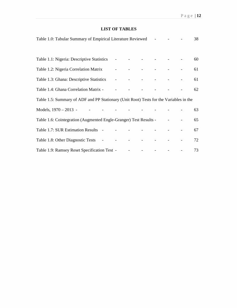
LIST OF TABLES

Table 1.0: Tabular Summary of Empirical Literature Reviewed - - - 38

Table 1.1: Nigeria: Descriptive Statistics - - - - - - 60

Table 1.2: Nigeria Correlation Matrix - - - - - - 61

Table 1.3: Ghana: Descriptive Statistics - - - - - - 61

Table 1.4: Ghana Correlation Matrix - - - - - - - 62

Table 1.5: Summary of ADF and PP Stationary (Unit Root) Tests for the Variables in the

Models, 1970 – 2013 - - - - - - - - - 63

Table 1.6: Cointegration (Augmented Engle-Granger) Test Results - - - 65

Table 1.7: SUR Estimation Results - - - - - - - 67

Table 1.8: Other Diagnostic Tests - - - - - - - 72

Table 1.9: Ramsey Reset Specification Test - - - - - - 73

P a g e | 13

ABSTRACT

This study investigates the effects of budget deficits on selected macroeconomic variables in Nigeria and Ghana using annual time-series data of both economies covering from 1970 to 2013; and taking previous empirical studies as its point of departure. The specific objectives of the study include: to examine the effects of budget deficits on interest rates, inflation, and economic growth in Nigeria and Ghana within the methodological framework of Seemingly Unrelated Regression (SUR) model and Two-Stage Least Squares (2SLS). The study employs Eagle-Granger Cointegration test, Augmented Dickey Fuller (ADF) and Phillips-Perron (PP) tests in estimating the systems equations. Data sourced from World Bank, IMF - World Economic Outlook, Central Bank of Nigeria, Bank of Ghana and others, were analyzed using SUR model with several diagnostic and specification tests to examine the objectives of the study. From the perspective of this study, the empirical findings demonstrated that budget deficit has statistically negative effects on interest rate, inflation, and economic growth for both economies thereby supporting the neoclassical argument in the literature that budget deficit slows growth of the economy through resources crowding-out. Based on the empirical findings, many recommendations were made for both Nigeria and Ghana economies one of which stated that the government of Nigeria and Ghana should be mindful of the sources of financing the budget deficits so as to effectively manage the economic fluctuations and increase activities in the real sector. Also, it was recommended that both economies should pursue policies that will boost production of goods for both domestic consumption and exports in the long run through a combination of import substitution and export promotion strategies.

P a g e | 14

CHAPTER ONE

INTRODUCTION

1.1 Background of the Study

Budget deficit and its effects on macroeconomic variables is one of the most discussed issues

amongst economists and policy makers in both developed and developing countries (Saleh,

2003; Aisen & Hauner, 2008; Georgantopoulos & Tsamis, 2011). Intuitively, it is a

commonplace to construe that huge budget deficits have adverse macroeconomic effects such

as high interest rates, current account deficits, inflation, exchange rates volatility, with

implications on growth and development (Bernheim, 1989).

The budget deficit effects could either be negative, positive or a no positive or negative

relationship on macroeconomic variables. Budget deficit and its effects on any given

economy could be attributable to different methodologies countries employed and the nature

of data used by different researchers as most of the studies regress the macroeconomic

variable(s) on the fiscal deficit or the deficit on the macroeconomic variable(s)(Anyanwu,

1997).

Budget deficit refers to government expenditure exceeding government revenue over a period

of time (Anyanwu, 1997). When a deficit occurs in a country, it becomesimperative to find

remedy for financing such deficits so as to eradicate its negative implications. Nigeria and

Ghana as a developing economies have blamed prolonged economic crisis as one of the

major causes of budget deficit(s) in both economies as it has resulted in over indebtedness

and debt crisis, high inflation, poor investment performance and growth (Ezeabasili,

Mojekwu & Herbert, 2012). In Nigeria, public expenditure has led to increase in the fiscal

imbalances that siphon funds from the private sector investment, retarding growth and

reducing standard of living (Mpia & Ogrike, 2014). Fiscal imbalances create potential large

P a g e | 15

burden on future generations as workers may be forced to finance unfunded social

programmes. Budget deficits, therefore, lead to incurring debts which is a stock of liabilities

of the government (Udu & Agu, 2000). Budget deficit is generally associated with recession

because of the effect on revenues and expenditures (Dernberg, 1985).

The Ghanaian economy embarked recently, on the second leg of its centenary of

independence and democracy, announcing bold objectives that included an accelerated gross

domestic product (GDP) growth rate of 8% in 2009 and 10% before 2015 and achievement of

middle-income status of US$1000 dollars per capita by 2015 (Ackah, Aryeetey & Aryeetey,

2009). In the five decades since her independence from British rule in 1957, Ghana has gone

through different cycles of growth, marked by poor economic performance and military coup

d’états through to the 1980s. National economic policies during this period were often devoid

of market principles, and characterized by frequent price and income controls. At best, the

economy muddled through, with low productivity, high and volatile prices, an overvalued

currency and high interest rates (Ndulu & Connell, 2008).

The choice of this study which brought the economies of Nigeria and Ghana into focal point

for empirical investigation is formed by a number of reasons. Besides the obvious reason that

both economies share similarities in political and economic structures, the economies have

experienced very large fluctuations in the government budget deficits and high accumulation

of foreign debt, poor export performance, huge service account deficits, external debt

amortization, low inflow of foreign direct investment, misappropriation of external funding

support, excessive domestic monetary and credit expansion; price distortions and a

deterioration in the terms of trade (Ogiogio, 1996; & Obioma,1998).

In Nigeria, available data from the CBN (2012) statistical bulletin, show that deficit of -

8.62% of GDP was recorded in 1970 which rose to a surplus of 2.58% of GDP in 1971 and

P a g e | 16

declined to -0.82% of GDP in 1972. In 1974, Nigeria experienced a remarkable improvement

in the overall fiscal balances from 1970 to 2013 as surplus rose from 1.92% of GDP in 1973

to a surplus unit of about 9.54% of GDP. The Nigeria overall fiscal balance deteriorated

between 1980 and 1994 and recorded greater deficit of about -12.44% of GDP in 1982 on the

average. However, between 1995 and 2013, the Nigerian economy recorded a surplus of

about 1.19% of GDP on the average in 1996 with other years experiencing different deficit

percentages to GDP.

In Ghana, there has been huge and continuous deterioration in government fiscal position.

The economy has been in a persistent tendency towards budget deficit since independence as

a result of over expanding government expenditure, inadequate revenue generation capacity

of government and increasing debt levels (Pomeyie, 2001). The available statistics from

World Bank (2014) show that the Ghanaian economy has not recorded any surplus since their

independence and between 1970 and 2013.It is evidenced that the trends of the overall fiscal

balances of Ghanaian economy between 1970 and 2012 has been on the deficit side with a

huge deficit records of about -10.79% of GDP and -12.12% of GDP in 1982 and 2012

respectively. Apart from the period between 1981 and 1990 when there was remarkable fiscal

discipline, the government budget was consistently in deficit in the 1990s. On average, the

deficits was more than 5% of GDP in 1993.

As the economy of Ghana grows, policy makers have been concerned with the extent to

which the budget deficit is sustainable, and its effects on macroeconomic variables. However,

a deficit policy plays a vital role in assisting countries to achieve macroeconomic stability,

poverty reduction, income redistribution and sustainable growth. For this reason, most

governments use the budget as effective tool in achieving their economic objectives. This

means that large and accumulating budget deficit may not necessarily be a bad policy

objective if such deficits are effectively utilized to enhance economic growth. It is in line

P a g e | 17

with this that an appropriate operational definition and measure of budget deficit must be

clearly stated. Otherwise, the occurrence of large nominal budget deficit may be misleading

depending on the operational measure adopted by a particular country (Antwi, & Mills,

2013).

In Nigeria, the economy was caught in the deficit trap since early 1980s when the world oil

market collapsed, and since then, there have been frantic efforts to exit the trap but all to no

avail(Wosowei, 2013). Nevertheless, the fiscal policy adoption of Nigeria and Ghana in

financing deficits are attributable to major factors causing rapid monetary growth, exchange

rate depreciation and rising inflation. Thus the motivation for this study is to examine the

short and long run effect of budget deficit on interest rate, inflation and economic growth in

Nigeria and Ghana.

1.2 Statement of the Problem

Different schools of thought have demonstrated their opinions on budget deficits. Most

common are the Keynesian and the Ricardian Schools of Thought. While the Keynesian

posits that budget deficit affects mainly macroeconomic variables, Ricardian School refutes

the proposition (by the Keynesian school) and posits that budget deficits do not affect mainly

macroeconomic variables. However, budget deficit in developing economy like Nigeria and

Ghana plays a pivotal role in achieving economic and social objectives including

macroeconomic stability, sustainable growth and poverty reduction.

In recent times, the deficit positions of the Ghanaian budgets have worsened, drawing

attention to its long term sustainability (Bank of Ghana, 2005). As the two countries (Ghana

and Nigeria) consistently operate budget deficits, this lead to accumulation of government

debts. As past deficit adds up to current borrowings, it creates higher interest payments,

raising inflation with high volatility in real interest rate, depreciates exchange rate and retards

P a g e | 18

growth. This calls for further borrowing to cover the interest payment and the increasing

primary deficit which affects the rate of future borrowing.

Figure 1.1 Graph showing Inflation and Budget Deficit interactions in Nigeria (1970 -

2013)

Source: Researcher’s computation using data from CBN Bulletin of various years As seen in figure 1.1 above, the greater percentage of the overall budget balance in Nigeria

were on the deficit side with high inflation rate and unstable real interest rate. In 1990s the

average inflation rate soared to 72.8%. But, by 2007, the economy experienced a sharp

average fall of 6.57% in the inflationary trend.The interactions of real interest rate and budget

deficits in the figure 1.3 clearly distinguish between inflation and real interest rate.

In Ghana, the stock of government debt to GDP has been rising steadily from 17.2% in 2006

to 24.9% in 2007 and to 28.1% in 2008 (Bank of Ghana, 2007). Clearly, Ghana cannot use

new borrowing indefinitely to finance interest payments since changes in taxes and

government spending is followed by adjustment in future taxation and spending (Luporini,

1999).

-20.00

0.00

20.00

40.00

60.00

80.00

% of GDP

Year

Budget Deficit (% of GDP), and Inflation in Nigeria

BD(% of GDP) INFL

P a g e | 19

Figure 1.2 Graph showing, Inflation, and Budget Deficit interactions in Ghana (1970 -

2013)

Source: Researcher’s computation using data from World Bank, WEO Database, (2014)

In figure 1.2 above, Ghana recorded a deficit of -7.05% of GDP on the average in 1981 with

inflation soaring to about 117.8%. In 1982, budget deficit worsen on the average of -10.79%

of GDP with low inflation of about 21.3%. This shows that even if Ghana meets its interest

payment on debt by borrowing more, it must roll over its debt indefinitely because tax

revenue is not enough to pay for other expenditure. This has led to growing debt and

increasing tax rate.

Generally, in the case of Nigeria and Ghana, it has been claimed thatthe main causes of these

high rates of inflation were the widening fiscal imbalances, sources of deficit financing,

economic growth and the depreciation of the exchange rate. Nonetheless, the transition to

high inflation rates over the period resulted in substantial real cost and large losses in income,

at the same time as the performance of the economy as a whole declined as a result of

widening fiscal deficits and exacerbated by poor macroeconomic management and political

uncertainty(Arestis & Sawyer, 2006).

P a g e | 20

Nevertheless, empirical studies on the effects of budget deficit on macroeconomic variables

such as interest rate, inflation and growth seem not to lay credence on Keynesian proposition

or Ricardian Equivalence Hypothesis (REH). The major trust of this study is to examine the

short and long-run effect of budget deficits on interest rate, inflation and economic growth in

Nigerian and Ghana. This is necessitated by the fact that the previous empirical studies in this

area have no conclusive evidence in support of Keynesian-Ricardian paradigms in Nigeria

and Ghana. This is because, none of the previous studies conducted on the effects of budget

deficits in both economies used all the relevant variables and a few do not employ the

appropriate methodology. This is one of the motivations behind this study.Hence, this study

departs from previous studies due to the inclusion of relevant variables and thus employs the

most appropriate and robust methodology to explore the budget deficits and how it affect the

selected macroeconomic variables of these economies in both short and long run.

Against this background, the study contributes to the large body of the existing literature on

fiscal policies in Nigeria and Ghana in two ways. First, unlike many empirical studies, the

study employs a more vigorous and robust approach; the Seemingly Unrelated Regression

(SUR) model to analyze the effect of budget deficit on the selected macroeconomic variables

in Nigeria and Ghana over the period covering from 1970 to 2013. Second, the study

provides empirical evidence for the economies with recent fiscal policies for which

researches have not been conducted recently. Besides, previous studies have advanced in

characterizing the implications of alternative sources and composition of deficits spending

without investigating the effects of budget deficits on the selected macroeconomic variables

in the two economies.

1.3 Research Questions

In the light of the above discussions, the following research questions shall be addressed:

i. What are the effects of budget deficiton interest rate?

P a g e | 21

ii. What are the effects of budget deficit on inflation?

iii. Does budget deficit have any impact on economic growth?

1.4 Objectives of the Study

The broad objective of this study is to investigatethe short and long run effects of budget

deficits on selected macroeconomic variables in Nigeria and Ghana. Specific objectives of

the study are:

i. To examine the effects of budget deficits on interest rates in Nigeria and Ghana.

ii. To ascertain the effects of budget deficits on inflation in Nigeria and Ghana.

iii. To evaluate the effects of budget deficits on economic growth in Nigeria and Ghana.

1.5 Hypotheses of the Study

In view of the above research questions, the following hypotheses are formulated in order to

ascertain the answers to the questions:

H01: Budget deficitshavenosignificant effects on interest rate in Nigeria and Ghana.

H02: Budget deficitshavenosignificant effects on inflation in Nigeria andGhana

H03: Budget deficits have no significant effects on economic growth in Nigeria and Ghana.

1.6 Policy Relevance of the Study

Developing economies like Nigeria and Ghana are in search of long-term policies not only

for macroeconomic stabilization but also for sustainable economic growth and development.

The private sector has always mourned that the fiscal deficit and its inflationary financing has

led to a slow-down in economic activity. There is need for a comprehensive study which

exposes the dynamics of the government fiscal deficit and its effects on the economy. This

study is designed to investigatethe short and long run effects of budget deficits on some

selected macroeconomic variables in Nigeria and Ghana. An academic study such as this is

P a g e | 22

crucial to both the Nigerian and Ghanaian economy in ascertaining the extent to which

budget deficit affects some macroeconomic variables in both short and long run. However,

the justification of this study is that it will add value to policy making especially in fiscal

adjustment and macroeconomic management. The findings of the study will also assist policy

makers to understand the centrality of the government fiscal deficit in policy formulation. It

is further hoped that the findings of the study will assist policy makers to place the right

emphasis on the role of fiscal adjustment in economic policy.

Furthermore, given the Keynesian-Ricardian dichotomy on budget deficit, it is needful to

investigate the effects of budget deficits on some selected macroeconomic variables in

Nigeria and Ghana. As a result, this research work seeks to contribute to the ongoing debate

on the relationship of budget deficits and some selected macroeconomic variables in Nigeria

and Ghana. Therefore, policy makers, experts, institutions, government agencies, researchers

and students in areas of public sector economics, development economics, international

economics, and econometrics are likely to find the outcome of this study very useful.

1.7 Scope of the Study

The study, as stated abinitio tends to investigate the short and long run effects of budget

deficits on selected macroeconomic variables in Nigeria and Ghana. It is pertinent to note that

the nexus between budget deficits and macroeconomic variables are still not well ascertained

especially when viewed in both short and long run. However, the study covers from 1970 to

2013. The range is chosen to ensure high level of degree of validity and precision in the

study. The variables of interest which are used to investigate the short and long run effects of

budget deficits on the selected macroeconomic variables in Nigeria and Ghana are: budget

deficit, interest rates, inflation,exchange rate depreciation, government expenditure, money

supply (M2), total savings, and real GDP.

1.8 Conceptual Framework

P a g e | 23

Awe and Funlay (2014) state that budget deficit occurs when government expenditures

exceed its revenues, thus the level of public savings is negative. This may harm the economic

growth of a country. Budget deficits lead to incurring debts which is a stock of liabilities of

the government (Keating, 2000). Budget deficit is a situation where the government budgets

to spend more than it intends to collect as revenue (Udu and Agu, 2000). Dernberg (1985)

posits that budget deficits are generally associated with recession because of the effect on

revenues and expenditures.

Fiscal deficit has gathered substantial attention in the literature in the area of macroeconomic

theory due to its impact on the macroeconomic variables. When budget deficit is financed by

borrowing, it expands government’s demand for credit through competition with households

and business firms (Hyman, 1994). This puts upward pressure on interest rate and slows

down the rate of capital formation. In Keynesian models, this occurs through a rise in real

interest rate which reduces investment purchases through the transmission mechanism.

However, this depends on the responsiveness of interest rate to increased demand for credit

and the reaction of private investors to higher interest rate. For instance, if investment

demand is unresponsive to changes in interest rate, the effect on investment will be very

small. Also, if the economy is in deep recession, any extra borrowing by government may put

little upward pressure on interest rate because the supply curve for funds will be quiet flat.

Yet, if the return on private investment exceeds the return on government investment

particularly on infrastructure, the rise in public investment would crowd in private investment

(Barua, 2005).

Also, large budget deficit increases the debt crisis in terms of its services and levels. As the

national debt grows, interest payment also grows which serves as tax on investment. This

reduces private investment, increases unemployment, lowers tax revenue and leads to higher

future deficits. Hence, the economy continues to incur mounting debts which may lead to its

P a g e | 24

collapse. Most countries trapped in debt servicing difficulties did run huge budget deficits at

some point in time. Yet, it is argued that public debt growth compels government to target

higher economic growth and revenue in order to finance any rising debt obligations.

Otherwise it will force the economy into a deficit trap (Barua, 2005).

On the burden of future generations, most economists agree that financing budget deficit

through external debt means the postponement of tax increases. However, it is asserted that

such burden depends on how the contracted loan is utilized. If the funds are spent on current

consumption expenditure, future generations are likely to be worse-off but if spent on

productive activities such as education and health then future generations are likely to be

better-off (Mankiw, 2003).

In addition, if budget deficit is monetized, it increases aggregate demand through increase in

government purchases without a corresponding increase in taxes. Hence, governments need

to run fiscal deficit particularly in the early stages of development to lead the economy in the

path of growth and development (Xiomara & Greenidge, 2003). Secondly, it increases money

supply. This exerts downward pressure on interest rate and upward pressure on equilibrium

money stock and price level unless the economy is in deep recession. This leads to higher

inflation, uncertainty and instability of real interest rate which tends to lower real tax revenue.

Hence, monetized deficit should be kept low and effectively managed in the short-to-medium

term (Bebi, 2000; Turnovsky, 2000).

Causes and Determinants of Budget Deficit Growth

In general, changes in budget deficit is attributed to changes in government spending or tax

revenue or both. Government receives revenue in its daily transactions and on capital items in

the form of taxes and interests. On the other hand, government pays for daily activities and

capital items such as administrative expenses, loans and grants. Thus, budget deficit increases

when government spending persistently exceeds its revenue. If expenditure continue to mount

P a g e | 25

up throughout the years whereas revenues especially taxes are poorly collected, it widens the

budget deficit position of the country. In this case, the accumulated value of past deficit

creates increase debts which must be financed together with the accompanying interest

payments.

With reference to political-economic models of government behaviour, it is recognized that

incumbent administrations tend to stimulate their economies on the eve of political elections

through tax cuts, increase spending and transfer payments. This occurs in countries where

political power changes frequently between rival parties. In such cases, each rival

administration spends over and above its budget and deliberately wait until after election

before implementing policies to reduce the deficit. These ad hoc policies tend to widen the

overall budget deficit and debt levels of the countries (Sachs & Larrain, 1993).

However, the extent of the impact of budget deficit on an economy is blamed by

macroeconomic factors such as expected inflation, cyclical position of the economy which

influences tax revenues and changes in expenditure. Theory predicts that cyclical fluctuations

in output which is caused by economic boom and/or recession impact significantly on budget

deficit. In periods of recession when output is low, budgets tend to be in deficit because direct

taxes fall sharply due to contraction in tax base. Also, certain categories of government

spending become countercyclical and rise during business cycle downturn. Yet, such

fluctuations in output growth are endemic in free market economies (Gebhard & Silika,

2006).

Budget Deficit Growth and Economic Sustainability

Financing of budget deficit in Ghana and other developing economies like Nigeria have had

diverse macroeconomic burden on the economy (Antwi et al, 2013). For instance central

bank financing of budget deficit have expanded the monetary base and money supply.

P a g e | 26

According to Wetzel and Roumeen (1991) central bank financing of budget deficit in Ghana

has distorted the distinction between monetary and fiscal policies whereas the sale of

domestic bond increased interest rate and this has led to increase in the net domestic

financing from 0.49 percent of GDP in 2004 to 4.15 percent in 2006. As a result, money

supply (currency and deposits) increased from 6.84 percent in 2005 to 34.4 percent in 2006,

and thus the domestic interest and bank rate reduced due to low demand for bonds (ISSER,

2007). Also, Ghana has accumulated large external debt and so borrow externally only on

short term bases at high interest rate. This is because foreign financing raises the cost of

servicing external debt. For this reason, Ghana’s access to external borrowing prior to 1984

had been limited, ranging between -0.74 and 1.62 percent of GDP. In recent times however,

debt levels have been falling. External debt fell from 72.5 percent in 2004 to 26.9 percent in

2006 with debt service to GDP reducing from 6.8 percent in 2004 to 6.0 percent in 2006

(Wetzel and Roumeen, 1991: 48; ISSER, 2007)

1.9 Structure of the Study

This study will be organized in five chapters. Following this introduction as Chapter 1,

Chapter 2 presents a review of literature on both thetheoretical and empirical evidences.

Chapter 3 discusses the methodology used in the study, Chapter 4 presents the analysis and

interpretation of the results obtained using the methodologies in previous chapter. Finally,

Chapter 5 highlights the conclusion and recommendations on fiscal policy management in the

Nigeria and Ghana.

P a g e | 27

CHAPTER TWO

REVIEW OF RELATED LITERATURE 2.1 Review of Theoretical Literature

This section reveals the theoretical framework related to budget deficit and macroeconomic

variables. Some of the economist such as Keynesian, Neoclassical and Ricardian Schools of

Thought gave either positive or negative support to the relationship between budget deficits

and macroeconomic variables.

2.1.1 Budget Deficits, Crowding In and Crowding Out Effects Schools of Thought

In analyzing the literatures on the relationship between budget deficits and macroeconomic

variables, Bernhein (1989) provides a brief summary of the three paradigms, and the cursory

of the paradigms are presented below.

The Neoclassical School

The neoclassical school proposes an adverse relationship between budget deficits and

macroeconomic variables. They argue that budget deficits lead to higher interest rates,

discourages the issue of private bonds, private investments, and private spending, increases

inflation level, and cause a similar increase in the current account deficits and finally slows

the growth rate of the economy through resources crowding out.

P a g e | 28

The Neoclassical school considers individuals planning their consumption over their entire

cycle. By shifting taxes to future generations, budget deficits increase current consumption.

By assuming full employment of resources the neoclassical school argues that increased

consumption implies a decrease in savings. Interest rate must rise to bring equilibrium in the

capital markets. Higher interest rates, in turn, result in a decline in private investment,

domestic production and an increase in the aggregate price level. Furthermore, Yellen (1989)

in Onuorah, and Ogomegbunam (2013) argues that in standard Neoclassical Macroeconomic

models, if resources are fully employed, so that output is fixed, higher current consumption

implies an equal and offsetting reduction in other forms of spending. Therefore, there will be

fully crowding-out of investment and/or net exports.

It is worth noting that it is important to distinguish between “financial” crowding out and

“resource” crowding-out. “Resource” crowding out occurs when the government competes

with the private sector on purchasing certain resources (skilled labour, raw materials and so

on). When the government sector expands, the private sector will contract because of the

increase in prices on these resources due to an excess demand by the government, hence this

leads to a fall in investment and consumption by the private sector. Thus the government

sector’s expansion crowds out the private sector. It is worth noting here as well that resource

crowding out is an important issue to take into account especially in developing countries

where resources are scarce even sometimes to the private sector, so any excess demand for

these resources by the government will severely impinge on private sector productivity.

The Keynesian School

The Keynesian economists propose a positive relationship between budget deficits and

macroeconomic variables. They argue that usually budget deficits result in an increase in

domestic production, increases aggregate demand, increases savings and private investment

at any given level of interest rate. The Keynesian absorptive theory suggests that an increase

P a g e | 29

in the budget deficits would induce domestic absorption and thus, import expansion, causing

current account deficit. In the Mundell-Fleming framework, an increase in the budget deficit

would induce an upward pressure on interest rate, causing capital inflows and an appreciation

of the exchange rate that will increase the current account balance.

The Keynesians provide a counter argument to the crowd-out effect by making reference to

the expansionary effects of budget deficits. They argue that usually budget deficits result in

an increase in domestic production, which makes private investors more optimistic about the

future course of the economy resulting in them investing more. This is known as the

“crowding-in” effect. It is worth noting here that the traditional Keynesian view differs from

the standard neoclassical paradigm in two fundamental ways. First, it permits the possibility

that some economic resources are unemployed. Second, it presupposes the existence of a

large number of liquidity-constrained individuals. This second assumption guarantees that

aggregate consumption is very sensitive to changes in disposable income. Many traditional

Keynesians argue that deficits need not crowd out private investment. Eisner (1989) suggests

that increased aggregate demand enhances the profitability of private investments and leads

to a higher level of investment at any given rate of interest. Hence deficits may stimulate

aggregate savings and investment, despite the fact that they raise interest rates. He concludes

that “evidence is thus that deficits have not crowded-out investment. There has rather been

crowding-in”. Heng (1997) utilized an overlapping-generations (OLG) model to provide a

theoretical framework to analyze the “crowding-in” issue of private capital by public capital.

He shows that public capital crowds-in private capital through two channels, namely, via its

impact on the marginal productivity of labour and savings, and via (gross)

complementarity/substitutability between public and private capital.

The Ricardian School

P a g e | 30

Finally, there is another contrary approach advanced by Barro (1989) known as the Ricardian

Equivalence Hypothesis (REH). Ricardian equivalence, or the Barro-Ricardo equivalence

proposition, is an economic theory which suggests that government budget deficits do not

affect the total level of demand in an economy. It was initially proposed by the 19th century

economist David Ricardo. In simple terms, the theory can be described as follows.

Governments may either finance their spending by taxing current taxpayers, or they may

borrow money. However, they must eventually repay this borrowing by raising taxes above

what they would otherwise have been in future. The choice is therefore between "tax now"

and "tax later". Suppose that the government finances some extra spending through deficits -

i.e. tax later. Ricardo argued that although taxpayers would have more money now, they

would realize that they would have to pay higher tax in future and therefore save the extra

money in order to pay the future tax. The extra saving by consumers would exactly offset the

extra spending by government, so overall demand would remain unchanged.

More recently, economists such as Robert Barro have developed more sophisticated

variations on the same idea, particularly using the theory of rational expectations. Ricardian

Equivalence suggests that government attempts to influence demand using fiscal policy will

prove fruitless. He argues that an increase in budget deficits, due to an increase in

government spending, must be paid for either now or later, with total present value of receipts

fixed by the total present value of spending. Thus, a cut in today’s taxes must be matched by

an increase in future taxes, leaving real interest rates, and thus private investment, and the

current account balance, exchange rate and domestic production unchanged. Therefore,

budget deficits do not crowd-in nor crowd out macroeconomic variables i.e. no positive or

negative relationship exists.

2.2 Thematic Issues

2.2.1 Budget Deficits in Ghana: An Overview

P a g e | 31

Ghana’s economy has maintained commendable growth trajectory with an average annual

growth of about 6.0% over the past six years. In 2013 growth decelerated to 4.4%,

considerably lower than the growth of 7.9% achieved in 2012. Growth has, however, been

broad-based, driven largely by service-oriented sectors and industry, which on average have

been growing at a rate of 9.0% over the five years up to 2013. Over the medium term to 2015,

the economy is expected to register robust growth of around 8%, bolstered by improved oil

and gas production, increased private-sector investment, improved public infrastructure

development and sustained political stability (African Economic Outlook, 2014).

According to AEO (2014), the continued widening budget deficit has been a major constraint

to fiscal and debt sustainability. Following an expenditure overrun in 2012, marked by an

unprecedented budget deficit of around 12% of GDP, the situation persisted in 2013, with

about the same level of budget deficit. Revenue enhancing and expenditure consolidation

measures underway in 2014 are expected to ease the fiscal deficit to 9%. In conjunction with

fiscal constraints, inflation has been on the rise resulting from a number of factors including

the removal of subsidies on petroleum prices and a gradual rise in electricity and water tariffs.

It is also worth noting the rise in public debt from 43% of GDP in 2011 to 48% in 2012, and

further to 53.5% in September 2013, resulting from a widened budget deficit. The external

sector will continue to experience a widened current-account deficit of around 12% of GDP

in 2014, exacerbated by a decline in commodity prices of major export commodities,

particularly on gold and cocoa.

2.2.2 Determinants of Budget Deficit Growth in Ghana

A model involving variation in inflation, government expenditure during wartime, cyclical

fluctuation in output during economic boom and recession in the postwar period was tested to

ascertain if it differs significantly from those during the world wars in the Swiss federal state.

The estimate showed some cyclical fluctuation in the world war periods. This supports the

P a g e | 32

assertion that significant determinant of budget deficit is increase in state expenditure during

wartime. In this case, civilian expenditure was reduced and/or taxes increased to finance

military expenditure during the war (Gebhard and Silika, 2006). In Ghana, changes in

inflation, interest rate and real GDP have reacted negatively to changes in budget deficit. For

instance, Antwi and Mills (2013) observed that high inflation in 1983 caused budget deficit to

increase by 35.8 percent due to decline in direct tax revenue. Also, changes in real interest

rate increased budget deficit by 11.3 percent of GDP in 1984. Again, high wage bill increased

the deficit by 2.5 percent in 1985. Thus, changes in macroeconomic variables have had strong

impact on the fiscal deficit in Ghana. However, these effects have become less pronounced

over the past years as the Ghanaian economy has grown more stable (Wetzel & Roumeen,

1991).

2.2.3 Fiscal Policy in Ghana

The government of Ghana is committed to fiscal consolidation with the ultimate objective of

reducing the budget deficit to around 5% of GDP by 2016. However, trend performance of

government operations continues to register widened budget deficit. Following an

expenditure overrun in 2012, marked by a significant budget deficit of around 6% of GDP,

the situation persisted in 2013 with a deficit of 7.8%. Fiscal measures implemented in the

second half of 2013 are expected to yield dividends in 2014. Key contributors to widened

budget deficit have been increased spending on wages and salaries, interest payments,

subsidies and arrear payments (African Economic Outlook, 2014).

According to AEO (2014), for the government of Ghana to address fiscal constraints

effectively, efforts should aim to raise tax revenue, in view of its substantial share (80%) of

total domestic revenue. Oil revenue is still low, accounting for just 0.2% of total revenue.

Grants from development partners are marginal and have maintained a diminishing trend,

accounting for only 7% of total revenues in 2013, down from around 14% in 2010. Despite

P a g e | 33

the marginal contribution of oil receipts, it is worth noting the distribution formula of such

receipts. In compliance with the Ghana Petroleum Revenue Management Act, about 30% of

total oil revenue to government is retained by the Ghana National Petroleum Commission

(GNPC) for the development of the oil and gas industry, while the remaining 70% is

appropriated through the Annual Budget Funding Amount (ABFA) and Ghana Petroleum

Funds (GPF) at around 40% and 60% respectively. While resources under ABFA are

reserved for funding priority projects, petroleum funds (GPF) are partly invested for future

generations through the established Ghana Heritage Fund.

2.2.4 Interest Rate Policy in Ghana

Interest rates were administratively controlled by the Bank of Ghana (BOG). The rationale

for the controls was that credit had to be cheap so as to promote investment and support that

favors borrowers (Daumont, Le Gall, & Leroux, 2004). It was the BOG that determined the

structure of the bank interest rates, which include the minimum interest rates for deposits and

maximum lending rates. Preferential lending rates were given to priority sectors such as

agriculture. The structure of interest rates determined by the BOG made no allowance for

loan maturity or risk; indeed, incentives for banks to extend credit were often perverse

because riskier sectors such as agriculture were accorded preferential inflation rates. In most

of the years, nominal interest rates were held below the prevailing inflation rates. However,

when inflation escalated in the middle of 1970s and the early 1980s, real interest rates were

highly negative (Antwi, 2009)

2.2.5 Fiscal Policy in Nigeria

Fiscal policy Management in 2012 and 2013 has centred on consolidation in order to ensure

macroeconomic stability. The fiscal deficit as a percentage of GDP has been estimated at -

1.8% in 2013, up from -1.4% in 2012, but well below the fiscal stance of a maximum of 3.0%

deficit enshrined in the Fiscal Responsibility Act. The Medium Term Expenditure

P a g e | 34

Framework (2014-2016)and Fiscal Strategy Paper proposed benchmark oil prices of USD 74,

USD 75 and USD 76 per barrel (pb) for 2014, 2015 and 2016 respectively. A benchmark oil

price of USD 77.5 pb was however set in the 2014 budget presentation to the national

assembly.

The 2012 budget was signed into law by the president of the Federal Republic of Nigeria in

April of the year following its passage into law by the legislative arm of government. The

level of implementation of the budget was 71.6%. The 2013 budget was signed into law by

the president in February, which was two months earlier than the preceding year as the

disagreement between the executive and the legislature over appropriation were resolved

early. The eventual implementation rate was around 70.0%. The ratio of capital expenditure

to total expenditure diminished to an estimated 23.9% in 2013 from 24.3% in 2012. The share

of capital expenditure on social community services (Health, Education and other allied

services) in the total rose from 10.0% in 2011 to 11.1% in 2012 while economic services

(agriculture and infrastructures) declined from 42.1% to 36.7%, respectively. The capital

component of Subsidy Reinvestment and Empowerment Programme (SURE-P) contributed

about NGN 272.5 billion, or USD 1.72 billion, thus raising the total capital expenditure to

NGN 2 059 billion (USD 13.03 billion) in 2013 (AEO, 2014).

In pursuance of fiscal prudence and the burgeoning debt profile, the government limits its

borrowing requirements in compliance with the Fiscal Responsibility Act (2007). Figures

from the Debt Management Office as at 31 December 2013 showed that Nigeria’s public debt

stock was USD 64.51 billion. Of this amount, the external debt of both the federal and state

governments was only USD 8.82 billion, of which the state governments constituted about

38.2%. The balance of USD 55.69 billion (about 86.3% of the total) drawn by both the

federal and state governments makes up the domestic debt component. In this regard, new

borrowing in 2014 is estimated to be NGN 572 billion (USD 3.62 billion), slightly down

from NGN 577 billion (USD 3.65 billion) in 2013 (AEO, 2014).

P a g e | 35

The observed persistent decline in oil revenues portends risk for fiscal policy and will shape

the trajectory of the medium-term fiscal outcome. Total revenue was on a declining trend

throughout 2013. It is noteworthy, though, that non-oil revenues have been rising

significantly over the same period, thereby compensating for the shortfall in oil revenues,

albeit inadequately. If the declining oil revenues are not contained and the rise in non-oil

revenues is not sustained, fiscal risks may set in. This could hinder the success of the

country’s ongoing reforms, and an overall negative impact on economic activities may result.

In addition, the government has been adjusting expenditures to accommodate the shortfall in

revenues. Capital expenditure, however, suffers huge downward adjustments because

recurrent expenditures, which are mainly salaries and overhead, can hardly be adjusted

automatically. These downward adjustments in capital expenditure may further slowdown

total economic activities and growth.

2.2.6 Macroeconomic Environmentsand Analytical Comparison between Nigeria and

Ghana

This section provides a review of economic developments in Nigeria and Ghana; and trends

in the major macroeconomic variables in recent years. The variables discussed in this section

include Gross Domestic Product (GDP), Inflation, the Value of Total Trade, Imports and

Exports.

The Nigerian economy faced numerous challenges which impacted overall economic activity

in 2012. Declines in the real growth rates of economic activity were experienced in both the

oil and non-oil sectors. Oil production was less than expected due to security challenges, and

floods which occurred in the latter part of the year, while the non-oil sector (notably

Agriculture, Wholesale & Retail Trade) was mostly affected by the floods and weaker

consumer demand (National Bureau of Statistics, 2013). The revised data for the NBS (2012)

indicates that real GDP grew by 6.34 % in the first quarter and 6.39% in the second quarter of

P a g e | 36

2012. The rate of economic activity was slightly higher than the initial estimates of 6.17%

and 6.28% respectively.

According to the Nigerian National Petroleum Corporation (NNPC), oil production was

estimated at 2.37 million barrels per day (mbpd) during the first half of 2012, as against

2.48mbpd produced in the first half of 2011. The 4.4% decline in crude production levels was

attributed to disruptions in production due to cases of oil theft and vandalization in the oil

producing areas. On the other hand, non-oil sector was affected by the incidence of flooding,

as well as muted consumer demand for the most part of the year, as seen in the Wholesale

and Retail Trade, Telecommunication and Post sectors while infrastructure challenges still

hampered Manufacturing. However, the Manufacturing sector did record a slight uptick in the

second quarter as a result of positivedevelopments in the power sector.

In Ghana, the economy is expected to slow down for the fourth consecutive year to an

estimated 3.9% growth rate in 2015, owing to a severe energy crisis, unsustainable domestic

and external debt burdens, and deteriorated macroeconomic and financial imbalances

(African Economic outlook, 2015). However, the provisional gross domestic product (GDP)

figures issued by the Ghana Statistical Services (GSS) further suggest that the economy

expanded by 4.2% in 2014, less than the growth of 7.3% recorded in 2013. The drivers of

growth continue to be the service sectors, which constitute 50.2% of the economy, followed

by industry and agriculture at 28.4% and 19.9% respectively (AEO, 2015).

High growth rates in Ghana over the recent years have been accompanied by the build-up of

macroeconomic imbalances. In 2014 current account and fiscal deficits widened to 9.2% and

10.4% of GDP respectively, and the rate of inflation averaged 17.0%. By the end of

December 2014, foreign reserves were at 3.2 months of import cover. The domestic currency,

the cedi (GHS) depreciated by over 30% in nominal terms over the first nine months of the

P a g e | 37

year compared to a depreciation of 4.1% during the corresponding period in 2013. The

continued growth in the budget deficit resulted in public debt increasing from 55.8% of GDP

in December 2013 to 67.1% of GDP by the end of December 2014. To address the

increasingly unsustainable fiscal and current account imbalances, the Ghanaian authorities

started negotiations for a stabilization programme with the International Monetary Fund

(IMF) that was expected to begin in early 2015(AEO, 2015).

According to National Bureau of Statistics(NBS) (2013) as at December 2012, the headline

inflation rate showed a general downward trend during the year, despite the economic

challenges that the country witnessed. From the 12.6% recorded in January (year- on-year),

the headline inflation rate reached12.9% in April and June before slowing to 11.3% through

September. It rose further to 12.3% in November before falling slightly to 12.0% in

December. As a result, the average inflation rate for the year stood at 12.2%. On a month-on-

month basis, the headline inflation rate rose sharpest in March (1.6%). The major sources of

inflationary pressure in 2012 still appear to be structural and infrastructural constraints.

Nevertheless, the removal of fuel subsidies early in the year, the devastating flood that

occurred in the third and fourth quarters of 2012 as well as seasonal effects also played major

roles in driving up prices at various times.

In Nigeria, as at the third quarter of 2012, the value of total Merchandise Trade for the

country was estimated at N20,885.4 billion over the first three quarters of the year. Compared

to levels recorded during the first three quarters in 2011, the value of total merchandise trade

had remained roughly unchanged, increasing marginally by 0.4%. The value of total

merchandise trade points to increasing exports over the period while imports have been on

the decline. Specifically, imports have continued to trend downwards since the second quarter

of 2011, while the value of exports which increased substantially in late 2011, dipped in the

P a g e | 38

first quarter of 2012, but picked up in the second and third quarters of 2012(National Bureau

of Statistics (NBS), 2013).

2.3 Empirical Literature

On the empirical front, there is a large body of literature documenting the effects (both short

and long run) of budget deficits on macroeconomic variables in both developed and

developing economies. This large body of literature on the topic could be divided into

international, and Nigerian-Ghanaian evidence for distinctive purposes; and thus logically

arranged in order of objectives of the study and year(s) in which the study was carried out.

2.3.1 International Evidence

Vamvoukas (1998) empirically examines the short and long-run effects of budget deficits on

interest rates for Greece using annual time series data from 1970 to 1990 within the

methodological framework of cointegration, ECM strategy, and several diagnostic and

specification tests. The estimation results support the Keynesian model of a significant and

positive relationship between budget deficits and interest rates

Gupta and Uwilingiye (2009) investigate the direction of temporal causality between budget

deficit and interest rate for South Africa using quarterly and annual data for the period of

1961 to 2005. The results show that budget deficit Granger causes interest rate in the

quarterly data. However, for the annual data, the study finds no causal relationship between

the budget deficit and the Treasury bill rate. The two variables are positively cointegrated for

both data frequency.

Similarly, Bonga-Bonga (2011) investigates the extent of the effects of the systematic and

surprise changes in budget deficits on the long-term interest rate in South Africa between

1960 and 2000 using vector autoregressive (VAR) techniques. The study finds a positive

P a g e | 39

relationship between the budget deficits and long-term interest rates. On the other hand,

Akinboade (2004) uses the LSE approach and Granger-causality methods to investigate the

nexus between budget deficit and interest rate in South Africa, the study finds no relationship

between the budget deficit and interest rates.

Mukhtar and Zakaria (2008) uses Granger Causality test and Error Correction Model (ECM)

to examine long run relationship between budget deficits and interest rates for Pakistan using

quarterly time-series data for the period 1960 to 2005. The regression results show that

budget deficits have no significant effect on nominal interest rates. The results equally reveal

that budget deficit-GDP ratio has significant positive impact on nominal interest rates.

Aisen and Hauner (2008)asses the relationship between budget deficits and interest rates in

60 advanced and emerging economies with a panel dataset spinning from 1970 to 2005.The

result shows a significant and positive relationship between budget deficits and interest rates.

The study also finds that the effects of budget deficits on interest rates varied by country

group and period. The resultequally shows that the effects were larger and more robust in the

emerging markets and in later periods than in the advanced economies and in earlier periods.

The study further reveals that the effect of budget deficits on interest rates depends on

interaction terms and is only significant under one of several conditions such as sources of

deficit financing (mostly domestically financed), and/or interact with high domestic debt; low

financial openness, and/or interest rates liberalization.

Noula (2012) examines the determination of fiscal deficit and nominal interest rate in

Cameroon using annual time series data from 1974 to 2009. The study employs a loanable

funds model to test for fluctuations in the economy budget deficits and nominal lending rates.

Moreover, the empirical assessmentcarried out using ADF test and Error Correction Model

reveals a significant positive association between budget deficits and domestic nominal

P a g e | 40

lending interest rate. Also, the result from the Pairwise Granger Causality test conducted

shows a bi-directional causality between budget deficits and nominal interest rate.

Guess and Koford (1984) utilizes the Granger Causality test to study the causal relationship

between budget deficits and inflation, GNP and private investment using annual time-series

data for seventeen OECD countries for the period 1949 to 1981. The results show that budget

deficits do not exert negative changes in these variables. In the same vein, Darrat (1985)

applies Ordinary Least Square (OLS) technique in examining empirically the linkage

between deficits and inflation in the US during the post-1960 period. The estimation results

show that both monetary growth and federal deficits significantly influenced inflation during

the 1960s and 1970s. In addition, the study concluded that federal deficits bore a stronger and

more reliable relationship to inflation than monetary growth.

Easterly and Schmidt-Hebbel (1993) analyze data from a sample of 10 countries and find

strong evidence that over the medium term, money financing of the deficit leads to higher

inflation, while debt financing leads to higher real interest rates or increased repression of

financial markets. Moreover, Tekin-Kuru and Ozmen (1998) examine the long run

relationship among budget deficits, money supply and inflation in Turkey. The results reveal

that while the endogeneity of supply of money and inflation reject the validity of the

monetarist view, lack of direct relationship between inflation and budget deficit repudiate the

pure fiscal theory explanations.

Darrat (2000) utilizes an Error Correction Model (ECM) to investigate if high budget deficits

have any inflationary consequences in Greece over the period 1957- 1993. The empirical

result shows that the deficit variable exerts a positive and statistically significant impact on

inflation in Greece. More also, Catão and Terrones (2005) find a strong link between fiscal

deficits and inflation using a sample of 107 countries over the period 1960 to 2001. Their

P a g e | 41

results show that, a 1 percent reduction in the ratio of the budget deficit to GDP is associated

with an 8.75 percent lower inflation rate.

Makochekanwa (2008)studies the impact of budget deficit on inflation in Zimbabwe for the

period 1980 to 2005. The study finds a positive and stable long run relationship between the

budget deficit, exchange rate, GDP and inflation. Habibullah, Cheah and Baharom (2011)

examine the relationship between budget deficit and inflation in thirteen Asian developing

countries using annual data for the period 1950 – 1999. The study employs Granger causality

test and their result shows the existence of a long run relationship between budget deficit and

inflation thus concluding that budget deficits are inflationary in Asian developing countries.

Ndashau (2012) adopts Granger causality techniques, augmented by vector error correction

model (VECM) to highlight the existence of a causality effect from inflation to budget

deficits scaled by the money base. However, the effect of budget deficits on inflation was not

statistically significant. On the other hand, Lin and Chu (2013) employ a dynamic panel

quantile regression (DPQR)model following the autoregressive distributive lag (ARDL)

regime to examine the extent to which fiscal deficits are inflationary in 91 countries between

1960 and 2006. The results of the study show that fiscal deficits are inflationary only in high

inflation countries.

Dwyer (1982) applies a Vector Autoregression (VAR) Model to test for the linkage between

government deficits and macroeconomic variables (such as prices, spending, interest rates

and the money stock) in the U.S. over the period 1952 – 1978. The results are consistent with

the hypothesis that there are no perceived wealth effects of predictable changes in

government debt held by the public and as a result, no effects of the debt on inflation. No

evidence is found that larger government deficits increase prices, spending, interest rates, or

P a g e | 42

the money stock. The study also shows that the reason for the decline in inflation rates can be

attributed to the decline of money growth despite borrowing.

Barro (1990; 1991) investigates the effects of tax financed government expenditure on

investment and output in a cross-sectional study of 98 countries over the period 1960-85. The

study reveals that the ratio of real government consumption to real GDP (gc/y) has a negative

association with growth and investment. The result shows that government consumption exert

no direct effect on private productivity, but lowers savings and growth through the distorting

effects from taxation or government-expenditure programs.

Karras (1994) studies the relationship between budget deficits and macroeconomic variables

in a Cross-sectional study involving 32 countries for the period 1950-1980, using OLS and

generalized least square (GLS). The results show that deficits do not lead to inflation, they

are negatively correlated with the rate of growth of real output and increased deficits appear

to retard investment. Similarly, Al-Khedir (1996) investigates the relationship between

budget deficits and macroeconomic performance of the G-7 countries for the period 1964-

1993 using VAR. The study reveals that budget deficits lead to higher short-term interest

rates in the 7 countries. However, the results show that deficits have no impact on the long-

term interest rates. The trade balance has been worsened by the budget deficit and economic

growth in all 7 countries.

Mugume and Obwona (1998) examine the interaction between fiscal deficits and other

macro-level variables for Uganda in the post reform period. The results show that the

unsustainability of the budget deficit has implications for public, external and monetary

sectors. In particular, the study finds a negative relationship between fiscal deficits and

economic growth. Also the study reveals that fiscal deficit is linked to inflation, exchange

rate depreciation and the widening of current account deficit.

P a g e | 43

Vuyyuri and Seshaiah (2004), study the interaction of budget deficit with other

macroeconomic variables (Nominal effective exchange rate, GDP, Consumer Price Index and

money supply) for India, using Cointegration approach and Variance Error Correction

Models (VECM) for the period 1970 – 2002. The study reveals that exchange rate, GDP,

consumer price index and money supply to be cointegrated. Also the study find a bi-

directional causality between budget deficit and nominal effective exchange rates. But the

results find no significant relationship between budget deficit and GDP, Money supply and

consumer price index. The results also show that the GDP Granger causes budget deficit.

Brownbridge and Mutebile (2007) analyze the impact of an increase in the fiscal deficit on

macroeconomic policy management and the fiscal sustainability in Uganda between 1980 and

2005. The study argue that aid funded deficits may have effects akin to the Dutch disease

through the appreciation of the exchange rate with adverse effects for export sector

competitiveness. In addition, Keho (2010) investigates the causal relationship between budget

deficits and economic growth for seven West African countries over the period 1980-2005.

The author finds mixed results with three out of the seven countries showing no evidence of

causality, one showing a unidirectional causality running from deficit to growth and the rest

showing two-way causality between budget deficits and economic growth.

Georgantopoulos and Tsamis, (2011) investigate the casual link between budget deficit and

other macroeconomic variables (Consumer Price Index (CPI), Gross Domestic Product

(GDP) and Nominal Effective Exchange Rate for Greece during the period 1980-2009. Their

findings reveal no link between the budget deficit and CPI but they find casual links between

budget deficit and GDP and Nominal Effective Exchange Rate.

Odhiambo, Momanyi, Othuon and Aila (2013)also study the relationship between budget

deficits and economic growth in Kenya for the period 1970 to 2007. The regression results

P a g e | 44

show a positive relationship between budget deficit and economic growth. Buscemi and

Yallwe, (2012) using GMM technique to test for the nexus between budget deficit and

economic growth using dataset of China, India and South Africa.The study shows that fiscal

deficit results are significant and positively correlated to economic growth and saving in

China, India and South Africa. However, the authors reveal that real interest rates are

negatively and significantly correlated with economic growth and saving. The main

conclusion by the authors is that, fiscal deficit affects the economic growth and saving

through the means financing the deficit.

On the other, Najid (2013) uses Granger-causality test in estimating the relationship between

budget deficit and economic growth of Pakistan using time series data for the period of 1971

to 2007. The result shows that bi-directional causality runs from budget deficit to GDP and

GDP to budget deficit. The study concluded by analyzing that Budget deficit has no role in

bringing back the economy of the country to a stable level of equilibrium.

Lwanga and Mawejje (2014) use a vector autoregressive (VAR) and vector error correction

model (VECM) approach, pairwise granger causality test, and variance decomposition

techniques in investigating the macroeconomic effects of budget deficits in Uganda for the

period 1999 to 2011. The cointegration results indicate that the variables under study are

cointegrated and thus have a long run relationship. Similarly, the results based on the VECM

reveal unidirectional causal relationships running from budget deficits to current account

balance, inflation to budget deficit and budget deficit to lending interest rates. But the results

show no causal relationship between gross domestic product (GDP) and budget deficits in

Uganda. The Pairwise Granger Causality test results reveal unidirectional causal relationships

running from budget deficit to current account, budget deficit to GDP, inflation to budget

deficit, and a bi-directional causal relationship between the current account balance and GDP.

P a g e | 45

The study concluded that budget deficits in Uganda are responsible for widening current

account deficit and raising interest rates

2.3.2 Nigerian-Ghanaian Evidence

Obi and Nurudeen (2008) empirically investigate the effects of fiscal deficits and government

debt on interest rate in Nigeria between 1970 and 2005 using Vector Autoregression

approach (VAR).The empirical findings of the study reveal that the explanatory variables

account for approximately 73.6 percent variation in interest rate in Nigeria. The estimation

also shows that fiscal deficits and government debt are economically and statistically

significant.

Chukwu (2009) employs Johansen and Juselius (2009) multivariate cointegration technique

and Vector Error Correction Model (VECM) to comparatively examine the causal

relationships between internal and external deficits using Nigerian quarterly and annual data

from 1971 to 2006. The cointegration test result suggests a long run stable relationship

between internal deficits and external deficits for both low and high frequency series. Thus

the study supported the Richardian Equivalence hypothesis for quarterly series but validates

the conventional Keynesian view for annual series.

Odionye and Uma (2013) employ augmented Granger causality test approach in examining

the relationship between budget deficit and interest rate in Nigeria using Vector Error

Correction model (VECM) for the period of 1970:1 – 2010:1. The results reveal that in the

long run co-integrating equation, budget deficit exert a positive and significant impact on

interest rate implying that a high budget deficit will increase interest rate in the country. The

result supports the Keynesian proposition. Also, evidence from Johansen co-integration result

indicates that there is a long run relationship between budget deficit and interest rate.

P a g e | 46

Sowa (1994) utilizes Error Correction Model (ECM) in estimating an inflation equation for

Ghana over the period 1963 - 1990. The study shows that inflation in Ghana is influenced

more by output volatility than by monetary factors, both in the long run and in the short run.

In Nigeria, Onwioduokit (1995) employs Granger causality test in investigating the causal

relationship between inflation and fiscal deficits using annual data from 1970 to 1994. The

variables in the empirical model are ratio of fiscal deficit to gross domestic product (GDP),

level of fiscal deficit and inflation rate. The study shows that fiscal deficit causes inflation

without a feedback effect but however feedback exist between inflation and the ratio of fiscal

deficit to gross domestic product.

Omoka and Oruka (2010) employ pair-wise Granger causality test in an attempt to offer

evidence on the causal long term relationship between budget deficit, money growth and

inflation in Nigeria using annual time-series data covering from 1980 to 2005. In considering

the broadest definition of money supply, the study reveal that money supply causes budget

deficit which means that the level of money supply in the Nigerian economy determines

whether there has been or there will be budget deficits. Inflation and budget deficit show a

bilateral or feedback causality proving that the changes that occur in inflation could be

explained by its own lag and also the lag values of budget deficit and in the same vein,

changes that occur in budget deficits are explained by its lagged values and the lagged values

of inflation. The implication of their findings is that both budget deficit and inflation could be

caused by money supply meaning that they are both monetary phenomena.

Oladipo and Akinbobola (2011) employ Granger causality pair-wise test in determining the

causal relationship between budget deficit and inflation in Nigeria. The study find that there

is no causal relationship from inflation to budget deficit but from budget deficit to inflation in

Nigeria. This indicates that budget deficit affects inflation through fluctuations in exchange

rate in the Nigerian economy.

P a g e | 47

Dockery, Ezeabasili and Herbert (2012) examine the long term relationship between fiscal

deficits and inflation for Nigeria using a modelling approach that incorporates the theory of

cointegration and employs vector error correction model. The empirical results show a

positive but insignificant relationship between fiscal deficits and inflation. The analysis of the

Nigerian data also indicate a weak link to previous levels of fiscal deficits with inflation and

provide, moreover, evidence of a positive long-run relationship between money supply

growth and inflation, suggesting therefore that money supply growth is pro-cyclical and tends

to grow at a faster rate than the rate of inflation. Similarly, from the impulse response and

variance decomposition analysis, the study finds that the length of inflation is an important

determinant of the ability of the system to return to its long-run equilibrium following a

shock.

Ozurumba (2012) employs Autoregressive Distributed Lag (ARDL) model and the Granger-

causality test in examining the causal relationship between inflation and fiscal deficits in

Nigeria covering the period 1970-2009. The result of the Granger-causality test shows that

the null hypothesis which says that fiscal deficit does not cause inflation should be rejected

since the result is significant with probability less than 0.05. This implies that fiscal

deficit/GDP causes inflation. However, no feedback mechanism exist between the variables.

The results from the ARDL test confirm a significant negative relationship between growth in

fiscal deficit (% of GDP) and inflation.

Akosah (2013) employs Ordinary Least Squares (OLS) in estimating the threshold effect of

Budget deficits on economic growth in Ghana using quarterly data from 2000 to 2012. The

study finds an inverse long run relationship between budget deficit and economic growth,

especially as the deficits have often been used to finance recurrent expenditures, suggesting

that high budget deficit, driven by recurrent expenditures, slows down economic growth. In

P a g e | 48

the short run, however, the result reveals that budget deficits promote economic growth, but a

deficit beyond the threshold level of 4% of GDP is detrimental to economic growth. This

result is robust and supports the West African Monetary Zone’s (WAMZ) primary fiscal

convergence criterion. The result also shows that fiscal restraint to the level below the

threshold will both stimulate a sustainable economic growth and overall stability in Ghana.

Larbi (2012) investigates the long-run impact of budget deficit on economic growth in Ghana

covering the period of 1980 to 2010 using Johanson cointegration procedure and Granger

Causality test. The empirical evidence from the Johanson cointegration test shows that budget

deficit exerts no significant long-run impact on economic growth. Further evidence from the

Granger Causality test conducted suggests significant positive long-run relationships between

the capital stock, openness, total government expenditure and growth rate with budget deficit

coefficient variable – positive and statistically significant.

Yaya (2010) utilizes the Granger-causality test using a sample of seven West African

countries namely; Benin, Burkian Faso, Cote d’ Ivoire, Mali, Niger, Senegal and Togo to

examine the causal relationship between budget deficits and economic growth in these

countries over a period of 26 years. The study reveals that in three countries, there exist no

causality between budget deficits and economic growth. The above findings indicate a two-

way causality in three countries, deficits having adverse effects on growth. Overall, these

results give support to the West African Economic and Monetary Union budgetary rule

aiming at restricting the size of budget deficit as a prerequisite for sustainable growth and real

convergence. In four other countries, there exist causality evidence between budget deficit

and economic growth implying that deficits retard economic growth rate. These findings have

two main implications. First, they lend support to the control of budget deficits within the

West African Economic and Monetary Union countries in order to increase domestic savings

and finance economic growth. Second, evidence of causality running from economic growth

P a g e | 49

to deficit makes difficult the control of budget deficit to depend on the aggregate

macroeconomic environment. In periods of recession, revenues are expected to decrease,

generating fiscal imbalance. In periods of expansion, revenues increases which leads to

reduction in the size of deficit.

Wosowei (2013) employs Ordinary Least Squares (OLS) in determining the relationship

between fiscal deficit and macroeconomic performance in Nigeria over the period 1980 to

2010. However, the empirical findings show that fiscal deficits even though it met the

economic a prior in terms of its negative coefficients, macroeconomic output is statistically

significant. The result also shows a bilateral causality relationship between government

deficit and gross domestic product, government tax and unemployment, while there is an

independent relationship between government deficit and government expenditure and

inflation.

Antwi and Mills (2013) evaluate budget deficit sustainability of Ghana between 1960 and

2010 using the present value budget constraint approach; employing annual time series data,

the Augmented Dicky Fuller and Philip-Parron tests for unit root rejected the null hypothesis

at 1 percent significance level after first difference. Hence, both government expenditure and

revenue of Ghana are stationary and integrated of order one. The Granger causality test from

the regression result supported a bi-directional causation such that both expenditure and

revenue of Ghana have temporal precedence over each other. This means past and present

values of government revenue provide important information to forecast future values of

expenditure. The test for cointegration favours the sustainability of budget deficit of Ghana at

10 percent significance level in the strong sense. The result equally shows that the Ghanaian

government can continue to service its past accumulated deficits without large future

correction to the balance of income and expenditure. Again, the study achieved the

P a g e | 50

conventional negative sign of the speed of adjustment to long run equilibrium following

shocks to the system at 5% significance level.

Bakare, Adesanya, and Bolarinwa (2014) empirically investigate the long term relationship

between budget deficit, money supply and inflation in Nigeria from 1975 to 2012 using

annual time-series data. The stationary test carried out using Augmented Dickey-Fuller

(ADF) reveals that the variables in the model are stationary at levels. However, the study

tested for a long run relationship among the variables using Johansen co-integration test

which also suggests that there are at least three co-integrating vectors among these variables.

Also, the estimated coefficient of the Error Correction Model shows that about 132% of the

errors in the short run are corrected in the long run. Thus the overall result between inflation

rate and growth of money supply, growth ratio of budget deficit to GDP and growth ratio of

external debt to GDP indicates that the specified model is statistically significant at 5% level.

Awe and Funlayo (2014) investigate the short and long run implications of budget deficit

oneconomic growth in Nigeria using time series data covering period of 1980-2011. The

result from the OLS regression analysis indicates that a negative relationship exist between

budget deficit and economic growth. The study also employs Johansen cointegration

technique in investigating the long run effect of budget deficit. The result shows that there is

a significant long-run relationship between budget deficit and economic growth in Nigeria.

The result from Error Correction Model reveals that budget deficit shows a negative

relationship with gross domestic product while gross capital formation (investment) shows a

positive relationship with GDP.

Oyeleke and Adebisi (2014) analyze the fiscal deficit sustainability of Ghana using Ordinary

Least Squares (OLS), Eagle-Granger and Error Correction Model procedures with annual

time series data covering from 1980 to 2010 to determine whether or not the economy has

achieved feat as a criterion required for membership in proposed West African Monetary

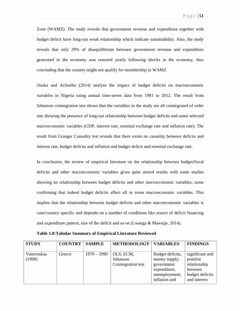
P a g e | 51

Zone (WAMZ). The study reveals that government revenue and expenditure together with

budget deficit have long-run weak relationship which indicate sustainability. Also, the study

reveals that only 29% of disequilibrium between government revenue and expenditure

generated in the economy was restored yearly following shocks in the economy, thus

concluding that the country might not qualify for membership in WAMZ

Osuka and Achinihu (2014) analyze the impact of budget deficits on macroeconomic

variables in Nigeria using annual time-series data from 1981 to 2012. The result from

Johanson cointegration test shows that the variables in the study are all cointegrated of order

one showing the presence of long-run relationship between budget deficits and some selected

macroeconomic variables (GDP, interest rate, nominal exchange rate and inflation rate). The

result from Granger Causality test reveals that there exists no causality between deficits and

interest rate, budget deficits and inflation and budget deficit and nominal exchange rate.

In conclusion, the review of empirical literature on the relationship between budget/fiscal

deficits and other macroeconomic variables gives quite mixed results with some studies

showing no relationship between budget deficits and other macroeconomic variables, some

confirming that indeed budget deficits affect all or some macroeconomic variables. This

implies that the relationship between budget deficits and other macroeconomic variables is

case/country specific and depends on a number of conditions like source of deficit financing

and expenditure pattern, size of the deficit and so on (Lwanga & Mawejje, 2014).

Table 1.0:Tabular Summary of Empirical Literature Reviewed

STUDY COUNTRY SAMPLE METHODOLOGY VARIABLES FINDINGS

Vamvoukas (1998)

Greece 1970 – 1990 OLS, ECM, Johanson Cointegration test

Budget deficits, money supply, government expenditure, unemployment, inflation and

significant and positive relationship between budget deficits and interest

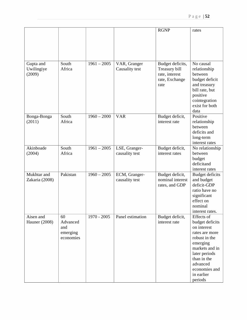
P a g e | 52

RGNP rates

Gupta and Uwilingiye (2009)

South Africa

1961 – 2005 VAR, Granger Causality test

Budget deficits, Treasury bill rate, interest rate, Exchange rate

No causal relationship between budget deficit and treasury bill rate, but positive cointegration exist for both data

Bonga-Bonga (2011)

South Africa

1960 – 2000 VAR Budget deficit, interest rate

Positive relationship between deficits and long-term interest rates

Akinboade (2004)

South Africa

1961 – 2005 LSE, Granger-causality test

Budget deficit, interest rates

No relationship between budget deficitand interest rates

Mukhtar and Zakaria (2008)

Pakistan 1960 – 2005 ECM, Granger-causality test

Budget deficit, nominal interest rates, and GDP

Budget deficits and budget deficit-GDP ratio have no significant effect on nominal interest rates.

Aisen and Hauner (2008)

60 Advanced and emerging economies

1970 - 2005 Panel estimation Budget deficit, interest rate

Effects of budget deficits on interest rates are more robust in the emerging markets and in later periods than in the advanced economies and in earlier periods

P a g e | 53

Noula (2012) Cameroon 1974 – 2009

ADF test, ECM, Pairwise Granger Causality, and Loanable Funds Model

Budget deficit, Money supply, RGDP, exchange rate, and foreign interest rate

Significant positive association between Budget deficit and interest rate

Guess and Koford (1984)

17 OECD countries

1949 – 1981 Panel estimation, Granger Causality test

Budget deficits Inflation, GNP, and Private Investment

Budget deficits do not cause changes in the variables

Darrat (1985) US 1960 – 1970 OLS Budget deficit, Inflation

Monetary growth and federal deficits significantly influence inflation in post 1960 period

Easterly and Schmidt-Hebbel (1993)

10 countries Panel data Panel estimation Budget deficit, inflation, real interest rates

Medium term money financing of the deficit leads to higher inflation, while debt financing leads to higher real interest rates

Tekin-Kuru and Ozman (1998)

Turkey VAR Budget deficit, money supply, Inflation

No direct relationship between budget deficit and inflation

Darrat (2000) Greece 1957 – 1993 ECM Budget deficit, inflation

Statistical significant and positive impact of budget deficit on inflation in short run

Catão and Terrones (2005)

107 countries

1960 – 2001 Panel estimation Budget deficit, inflation, GDP

positive impact of budget deficit on inflation

Makochekanwa (2008)

Zimbabwe 1980 – 2005 VAR Budget deficit, inflation, exchange rate, GDP

Significant positive impact of budget deficit on inflation in the

P a g e | 54

long run Habibullah, Cheah and Baharom (2011)

13 Asian developing countries

1950 – 1999 Panel estimation, Granger-Causality test

Budget deficit, inflation

Long run relationship exist between budget deficit and inflation, and budget deficits are inflationary in Asian developing countries

Ndashau (2012) OLS Budget deficits, inflation, exchange rates

Effect of budget deficits on inflation is not statistically significant

Lin and Chu (2013)

91 Countries

1960 – 2006 DPQR, ARDL Budget deficits, inflation, exchange rate

Fiscal deficits are inflationary only in high inflation countries

Dwyer (1982) US 1952 – 1978 VAR Budget deficits, interest rates, money stock

No effects of budget deficits on inflation, interest rates, and inflation

Barro (1990; 1991)

98 Countries

1960 – 1985 Panel estimation RGDP, Investment

The Budget deficit-RGDP has a negative relationship with GDP and investigate

Karras (1994) 32 Countries

1960 – 1980 OLS, GLS Budget deficit, inflation, investment, and RGDP

Budget deficit do not cause inflation, but negatively correlated RGDP

Al-Khedir (1996)

G-7 Countries

1964 – 1993 VAR Budget deficits, interest rate, trade balance, GDP

Trade balance has been worsen by the budget deficit and GDP in all the 7 Countries

Mugume and Obwona (1998)

Uganda Post reform period

OLS Budget deficit, GDP, inflation, exchange rate depreciation and Current account

Negative relationship between budget deficit and GDP

P a g e | 55

deficit Vuyyuri and Seshaiah (2004)

India 1970 - 2002 VECM Exchange rate, GDP, CPI and money supply

No significant relationship between budget deficit and GDP, Money supply and CPI

Brownbridge and Mutebile (2007)

Uganda 1980 – 2005

Keho (2010) 7 West African countries

1980 – 2005 Panel estimation, Granger-causality test

Budget deficit, GDP

3 countries shows show evidence of no causality, and 4 countries show two-way causality between budget deficits and GDP

Georgantopoulos and Tsamis (2011)

Greece 1980 – 2009 OLS, Granger-causality test

Budget deficit, CPI, GDP, nominal exchange rate

No link between budget deficit and CPI, but causal link exist among budget deficit, GDP and nominal exchange rate

Odhiambo, Momanyi, Othuon L, and Aila (2013)

Kenya 1970 – 2007 OLS, Granger-causality test

Budget deficit, GDP

Positive relationship between budget deficits and economic growth

Buscemi and Yallwe (2012)

China, India, and South Africa

1970 – 2007 GMM Budget deficit, real interest rate, GDP, saving

Budget deficit affects GDP and saving through financing the deficit. Also, real interest rates are negatively and significantly correlated with GDP and saving

P a g e | 56

Najid (2013) Pakistan 1971 – 2007 OLS, Granger-causality test

Budget deficit, GDP

Bi-directional causality Budget deficit to GDP, and GDP to budget deficit

Lwanga and Mawejje (2014)

Uganda 1999 - 2011 VAR-VECM, pair-wise granger-causality, variance decomposition

Budget deficit, inflation, interest rate, current account balance

No causal relationship between GDP and budget deficits. And bi-directional causal relationship between the current account balance and GDP

NIGERIAN-GHANAIAN EVIDENCE

STUDY COUNTRY SAMPLE METHODOLOGY VARIABLES FINDINGS

Obi and Nurudeen (2008)

Nigeria VAR Budget deficit, government debt, interest rate

Budget deficit and government debt are economically and statistically significant

Chukwu (2009) Nigeria 1971 – 2006 VECM, Johanson cointegration test

Internal and External deficits,

Long run stable relationship exist between internal and external deficits for both low and high frequency series

Odionye and Uma (2013)

Nigeria 1970:1 to 2010:4

VECM, Granger-causality test

Budget deficit, interest rate

Budget deficit exert a positive and significant impact on interest rate in the long run

Sowa (1994) Ghana 1963 - 1990 ECM, Johanson Cointegration test

Budget deficit, GDP, Money supply

Budget deficit has effect on GDP in both

P a g e | 57

short and long run

Onwioduokit (1995)

Nigeria 1970 – 1994 Granger-causality test

Budget deficit, GDP, inflation

Budget deficit causes inflation without feedback effect, but feedback effect exist between inflation and ratio of budget deficit-GDP

Omoka and Oruka (2010)

Nigeria 1980 – 2005 Pair-Wise test Budget deficit, inflation, money supply

money supply causes budget deficit; Inflation and budget deficit show a bilateral or feedback causality

Oladipo and Akinbobola (2011)

Nigeria Granger-causality pair-wise test

Budget deficit, inflation, exchange rate

No causal relationship from inflation to budget deficit, but from deficit to inflation

Dockery, Ezeabasili, and Herber (2012)

Nigeria VECM, Johanson Cointegration test

Budget deficit, inflation

Positive but insignificant relationship between budget deficit and inflation

Ozurumba (2012)

Nigeria 1970 – 2009 ARDL, Granger-causality test

Budget deficits, inflation

Significant and negative relationship between growth in fiscal deficit and inflation

Akosah (2013) Ghana 1990 – 2012 OLS Budget deficit, GDP, exchange rate

Negative relationship between budget deficit and GDP in the long run

Larbi (2012) Ghana 1980 – 2010 Johanson Cointegration and

Budget deficit, openness,

Positive long run

P a g e | 58

Granger Causality test

capital stock, government expenditure, growth rate

relationship between budget deficit and economic growth; and significant positive causality exist the capital stock, openness, total government expenditure & growth rate

Yaya (2010) 7 West African countries

26 years Granger-causality Budget deficit, GDP

no causality between budget deficits and GDP in 3 countries; and causality exist between budget deficits and economic growth in 4 countries

Wosowei (2013)

Nigeria 1980 – 2010 OLS, Granger-causality test

Budget deficit, GDP, unemployment, inflation, government expenditure and tax

Bi-lateral causal relationship betweenbudget deficit and GDP, government tax and unemployment

Antwi and Mills (2013)

Ghana 1960 – 2010 Present Value (PV) budget constraint approach, Granger-causality, ADF and PP tests

Budget deficit, interest rate, exchange rate, government expenditure and revenues

Bi-directional causation in both government expenditure and revenues

Awe and Funlayo (2014)

Nigeria 1980 – 2011 OLS, ECM, Johanson cointegration test

Budget deficit, GDP, investment

Long-run relationship exist between budget deficit and GDP, with negative correlation with growth, and positive with

P a g e | 59

investment.

Bakare, Adesanya, and Bolarinwa (2014)

Nigeria 1975 - 2012 ADF test, ECM, and Johanson cointegration test

Budget deficit, inflation, money supply, external debt

Long-run relationship exist among the variables, and thus statistically significant

Oyeleke and Adebisi (2014)

Ghana 1980 – 2010 OLS, Eagle-Granger, and ECM,

Government expenditure, revenue, and deficit

long-run weak relationship between government expenditure and revenue

Osuka and Achinihu (2014)

Nigeria 1981 - 2012 OLS, Johanson cointegration test, and Granger-causality test

Budget deficit, GDP, interest rate, nominal exchange rate and inflation rate

long-run relationship exist between budget deficits and some selected macroeconomic variables

SOURCE: Compiled by the Researcher

2.4 Limitation of Previous Studies and Value-To-Be-Added

There have been a number of studies on the effects of budget deficits on macroeconomic

variable(s) in both developed and developing economies evidenced from the empirical

literature reviewed.Based on the reviewed literature, one can conclude that the earlier studies

made significant contributions on the stock of knowledge as it relates budget deficits and

macroeconomic variable(s). Moreover, the earlier studies such as Sowa (1994), Vamvoukas

(1998), Uwilingiye and Gupta (2007) among others were considered a sine qua non for

generating the contemporary research interest on this topic and in these developing

economies - Nigeria and Ghana.

P a g e | 60

However, the literature discussed above shows that the effects of budget deficits (short or

long run) on macroeconomic variables are mixed and country case; and/or as a result of this,

the methodology and data employed in the empirical literature reviewed are foiled with

limitations. It is pertinent to take into cognizance that almost all the works reviewed were

single economy studies such as Onwioduokit (1995), Chukwu (2009), Bonga-Bonga (2011),

Antwi and Mills (2013), Osuka and Achinihu (2014) among others. Similarly, most of the

studies reviewed only consider either the short or the long run implications of budget deficits

on a particular or single macroeconomic variable; for instance, Vamvoukas (1998), Omoka

and Oruka (2010), Akosah (2013) among others. However, judging from the large body of

literature reviewed, no empirical study was found to have articulated both the short and long

run effects of budget deficits on the selected macroeconomic variables in these West African

countries - Nigeria and Ghana. Therefore, this study tend to fill this lacuna as well as add

more value to the literature by meticulously investigating the short and long run effects of

budget deficits on theselected macroeconomic variables in both Nigerian and Ghanaian

economies while paying particular andkeen attention on the country’s macroeconomic

environment so as to control for factors which was omitted in the literature.

Consequently, the study employs more robust technique – Seemingly Unrelated Regression

(SUR) model in investigating both the broad and specific research objectives.Also, the study

employs a longitudinal annual time-series and quarterly dataset spinning from 1970 to2013.

This is in sharp contrast to country specificNigerian or Ghanaian earlier studies conducted

which employed data ranging a shorter time period. To this objective, the study outlines a

modelling framework that links budget deficits to interest rate, inflation and economic growth

that captures the macroeconomic realities of the Nigerian and Ghanaian economies over the

period reflected by the available data.

P a g e | 61

Another important shortcoming of most previous studies which the current studyseeks to

overcome is that explicit attention was not paid to the time-series characteristics of the data

used. Using recent developments in time series econometrics as provided by Engle and

Granger (1987), Andrew (1991), Phillips and Peron (1988), Dickey and Fuller (1979), Newey

and West (1994), MacKinnon (1996),Johanssen (1991, 1995), Engsted and Bentzen

(2001),this studyis able to derive the relationship between the variables in themodel adopted.

CHAPTER THREE

RESEARCH METHODOLOGY

3.1 Theoretical Framework

To analyze the relationship between fiscal deficits and some selected macroeconomic

variables, it is helpful to begin with some national income accounting identities. The national

income account identity provides the basis for the relationship between budget deficit and

macroeconomic variables. This theoretical framework follows the work of Ezeabasili and

Mojekwu (2011). Under the fiscal approach to balance of payments; the government budget

balance is defined as the gap between revenues and expenditures. The above definition

derives from the national income identity, as:

P a g e | 62

Y = C + I + G + (X – M) …………………………………………………………. (1)

Where Y represents real GDP, C is private consumption, I stands for private investment, G is

government consumption, X and M stand for exports and imports respectively. Assuming the

aggregate demand A = C + I + G then Equation (1) can be rewritten as follows:

Y – A = X – M …………………………………………………………………….. (2)

Equation (2) reflects the behaviour of the external sector of the economy. The direct

interpretation is that, external imbalances always trigger a series of developments in the

economy, which in this case is budget deficit. Therefore, any attempt to restore the balance

must include effort to align revenue with expenditure. In order to isolate the disposable

income, tax (T) and international reserve (R) (the latter is introduced basically on the

assumption of the fixed exchange rate regime) are introduced into the national income

identity. It follows that Equation (1) will become:

Y + R – T = C + I + (G – T) + (R + X – M) ……………………………………… (3)

In the following equation, S (savings) is the disposable income minus private consumption.

That is: S = Y + R – T – C, the private absorption capacity is represented by (C + I), (G – T)

is for budget deficit, while the current account balance (CAB) is represented by (R + X – M),

R represents international transfer receipts and T stands for taxes. Substituting S and CAB by

their respective components, we get:

(S – I) + (T – G) = (R + X – M) ……………………………………………………. (4)

It is often argued that deficit in the current account occurs when aggregate investment

outweighs aggregate savings (Blanchard & Johnson, 2012; Abel & Bernanke, 2001; and

Mankiw, 2003). However, if investments equalssavings and government expenditure is

greater than its revenue then, the current account deficit becomes inevitable. The literature on

the current account is quite obvious when it indicates the degree at which the domestic

economy interacts with its external assets. Thus, (X + R – M) would also be equivalent to the

increase in net official assets plus the rate of capital outflow that is ∆NFA. Hence;

P a g e | 63

CAB = ∆NFA ………………..…………………………………………………….. (5)

The links between net savings of the private sector and the public sector deficit is easily

appreciated through the following illustration.

(S – I) + (T – G) = ∆NFA …………………………………………………………. (6)

The direct interpretation of the above equation assuming S = I is that:

(i) A budget deficit could be financed through a reduction in external net claims, which can

be done through increase in external public debt or reduction of international reserves in the

case of a fixed exchange regime. (ii) Budget deficit could also be financed domestically,

through increase in government debt held by the private economic sector. The relationship in

the banking system provides a clear understanding on how domestic borrowing is applied in

financing a budget deficit and the balance sheet is given as follows:

∆NFAb = ∆M2 - (∆DC g + ∆DC nb) …………………………………………........ (7)

The liability of the banking system is represented by M2 that is the broad money, ∆DC g is

domestic credit of the banking system to government and ∆DC nb is the credit of non-banking

sector (private sector) to the government. Equation (7) expresses the difference between

money expansion and credit expansion and, which works as follows. An increase in money

relative to credit expansion will reflect as an increase in the net foreign asset. In countries

where the capital markets are not advanced (such as Nigeria and Ghana), budget deficit is

usually financed through domestic and external borrowing. This expression can be simplified

as follows:

G – T = ∆DC g - ∆NFA g ………………………………………………………….. (8)

By substituting (8) into (7), the relationship between the financing of the budget deficit and

the banking system is brought to the fore. Thus:

G – T = ∆M2 - ∆DC nb – (∆NFA b + NFA g) ……………………………………… (9)

Equation (9) illustrates the sources through which government deficit can be financed. First,

by an increase in money (∆M2). Second, borrowing from non-banking sector. Lastly, by a

P a g e | 64

…….. (10)

reduction in international reserve or external borrowing. In all, increased budget deficit will

translate into increased current account deficit which precipitates new external borrowing or

draw down of external reserves. However, all the three means of financing a deficit may lead

to appreciation of real and nominal exchange rates under flexible exchange rate regime and

capital mobility.

3.2 Model Specification

Following the theoretical framework in section (3.1) above, the following models were

adopted;

Model I (for objective 1)

Haven laid the required theoretical foundations in the theoretical framework, the study links

the above stated foundations to specify our empirical models, thus the specification of the

interest rate model mirrors the works of Ariyo and Raheem (1991), cited in Tchokote (2004).

The specification of the model considers the following variables: Interest rate (INT) is the

dependent variable; while Government expenditure (GEX), budget deficit (BD), money

supply (MS), and inflation rate (INF) are the independent variable; µt is error term. The

model is represented as:

RIR = ƒ(GEX, BD, MS, INF)

The above relationship can be presented through a system of related equations by considering

a set of t linear equations for each t time points, and thus becomes:

RIR t1Ng = β01 + β1GEXt1

Ng + β2BDt1Ng + β3InMS t1

Ng + β4INF t1Ng + µt1

Ng

RIR t2Gh= β02 + β1GEXt2

Gh + β2BDt2Gh + β3InMS t2

Gh + β4INF t2Gh +µt2

Gh

Where: β0 = the intercept and, β1, β2, β3, β4 are the coefficients of the regression equation.

Ng, Gh = Ng: for Nigeria, Gh: for Ghana respectively

A priori, it is expected that the following relationship will occur; β1, β2, β4> 0; β3 < 0;

P a g e | 65

..... (11)

…. (12)

Model II (for objective II)

The second objective of the study is to examine the short and long run effects of budget

deficit on inflation in Nigeria and Ghana. Following the literature, we present an econometric

model similar to the work of Dockery and Ezeabasili (2012) which essentially is informed by

standard economic theory as evince in both Classical and Keynesian approaches.

Accordingly, a log linear inflation-fiscal deficit econometric model is specified as follows:

INF t1Ng = Φ01 + Φ1BDt1

Ng + Φ2InRGDP t1Ng + Φ3InMS t1

Ng + Φ4EXDEPt1Ng + γt1

Ng

INF t2Gh = Φ02 + Φ1BDt2

Gh + Φ2InRGDPt2Gh + Φ3InMS t2

Gh + Φ4EXDEPt2Gh + γt2

Gh

Where: INF = Inflation rate

BD = Budget deficits

MS = Money supply (M2)

RGDP = Real gross domestic product

EXDEP = Depreciation of the exchange rate

Ng, Gh = Ng: for Nigeria, Gh: for Ghana respectively

γt is a stochastic term.

(A priori, we expect the parameters: Φ1, Φ2, Φ3, Φ4> 0; Φ4> 0 or Φ4< 0).

Model III (for objective III)

The third objective of the study which states – short and long run effects of budget deficit on

economic growth in Nigeria and Ghana can be captured following the adoption of the work

of Awe and Funlayo (2014). The model is specified below:

GDP = ƒ(investment, savings, interest rate, budget deficit).

InRGDP t1Ng = α01 + α1INF t1

Ng + α2InSAV t1Ng + α3RIR t1

Ng + α4BDt1Ng + εt1

Ng

InRGDP t2Gh = α02 + α1INF t1

Gh + α2InSAV t2Gh + α3RIR t2

Gh + α4BDt2Gh + εt2

Gh

Where:

RGDP = Real Gross Domestic Product, a proxy for economic growth

P a g e | 66

INF = Inflation

SAV = Savings

INT = Interest rate

BD = Budget Deficit

α0 = the constant or the intercept

α1 – α4 = the coefficients of the explanatory variables

εt = Stochastic error term

(A priori, we expect the parameters: α1< 0, α2 > 0, α3< 0, α4 < 0 or α4 > 0)

3.3 Estimation Procedure

3.3.1 Empirical Models: Seemingly Unrelated Regression (SUR)

The SUR model is a generalization of multivariate regression using a vectorized parameter

model. The Y matrix is vectorized and vertically concatenated, yv. The design matrix, D, is

formed as a block diagonal with the jth design matrix, X j, is on the jj th block of the matrix.

The model is then expressed as:

E[Y(Nxp)]= { X1(Nxm1) β1 (m1x1) , X2(Nxm2) β2 (m2x1) , Xj(Nxmj) βj (mjx1) ,

Xp(Nxmp) βp (mpx1) ……………………………………………………………………. (13)

Where: mj is the number of parameters estimated (columns) by the j th design matrix, X j.

The SUR model is laid out in metric form as:

E(yv) D B

ŷI (Nx1)

XI 0 0 0 0 0 ᵝ1(mxl)

ŷ2 (Nx1)

(Nxm)

X2 0 0 0 0 ᵝ2 (m2xl) ……………. (14) E(yv) = … (Nxm… 0 0 0 ; (Npx1)

ŷj (Nx1)

x, 0 0 βj(mjx1) (sym) (Nxmj) 0 ŷp (Nx1

) (Nxmp)X

ᵝp(mpx1)

(Npx\ (NpxM) (Mx1) P where:

M is the total number of parameters estimated over the p models, M=∑mj.The (j=1)

P a g e | 67

[I N -Hi][I N - Hj]y j…..........….. (16)

parameter estimates are solved as:

B= [DIQ-ID] [D' Q-lyv]……………………………..… ..….. (15) (MxNp)(NpxNp)(NpxM) (MxNp)(NpxNp)(Npxl)

Q is weight matrix based on the residual covariance matrix of the Y variables and is formed

as:

Q = ∑⊗IN .The ijthelement of ∑is calculated as: (NpxNp) (pxp)

where: H, = Xj(X jXj) -1Xj is the hat matrix for the jth design matrix and df* is the average of

the numerator degrees-of-freedom (df) for the ithand jth models. Thus, a SUR model is an

application of generalized least squares (GLS). In fact, because the residual covariance

matrix is unknown and must be estimated from the data, this application is often called

feasible

generalized least squares (Timm, 2002).

3.3.1.1 Two Stage Least Squares and Instrumental Variables

Two-Stage least squares (2SLS) regression analysis is a statistical technique that is used in

the analysis of structural equations. This technique is the extension of the OLS method. It is

used when the dependent variable’s error terms are correlated with the independent variables.

Additionally, it is useful when there are feedback loops in the model (Angrist & Imbens,

1995).

Many economic models involve endogeneity: that is, a theoretical relationship does not fit

into the framework of y-on-X regression, in which we can assume that the y variable is

determined by (but does not jointly determine) X (Wooldridge, 2006). From a mathematical

standpoint, the difficulties that this endogeneity cause for econometric analysis are identical

to problems associated with omitted variables, and that of errors-in-variables, or

measurement error in the X variables. In each of these three cases, OLS is not capable of

P a g e | 68

delivering consistent parameter estimates. The general concept is that of the instrumental

variables estimator; a popular form of that estimator, often employed in the context of

endogeneity, is known as two stage least squares (2SLS) (Wooldridge, 2006).

Instrumental variable methods allow consistent estimation when the explanatory variables

(covariates) are correlated with the error terms of a regression relationship. Such correlation

may occur when the dependent variable causes at least one of the covariates ("reverse"

causation), when there are relevant explanatory variables which are omitted from the model,

or when the covariates are subject to measurement error. In this situation, ordinary linear

regression generally produces biased and inconsistent estimates(Bullock, Green & Ha, 2010).

However, if an instrument is available, consistent estimates may still be obtained. An

instrument is a variable that does not itself belong in the explanatory equation and is

correlated with the endogenous explanatory variables, conditional on the other covariates. In

linear models, there are two main requirements for using an IV:

• The instrument must be correlated with the endogenous explanatory variables,

conditional on the other covariates.

• The instrument cannot be correlated with the error term in the explanatory equation

(conditional on the other covariates), that is, the instrument cannot suffer from the

same problem as the original predicting variable.

3.3.2 Lag Length/Bandwidth Selection

Appropriate lag length/bandwidth shall be selected using coefficient of determination (R2),

Akaike Information Criterion (AIC), Schwarz information criterion (SC), Hannan-Quinn

information criterion (HQ), and Newey-West method criteria to determine the number of

lags/bandwidths in the series test.

P a g e | 69

3.3.3 Stationarity/Unit Root Test

In regressing a time series variable on another time series variable (s), one might obtain a

high R2 even though there is no meaningful relationship between the variables. This situation

shows the problem of spurious or nonsense regression (Gujarati, 2007). To test for a unit root

in the series, the Augmented Dickey-Fuller (ADF), as specified in Dickey and Fuller (1979),

and Phillips-Peron (Phillips and Peron, 1988) will be employed to ensure more robust results

in testing for the stationarity of the data in our models at level and at differences. However,

the test statistics of the Philips-Peron have the same distribution as those of Dickey-Fuller

with critical levels as provided by MacKinnon (1996). Thus, the model for the ADF is

specified below:

yt = µ + pyt-1 + εt ............................................................................................... (17)

Where µ and p are parameters and εt is assumed to be white noise, y is a stationary series if -

0< p < 1. If p =1, y is a non-stationary series; if the process is started at some point, the

variance of y increases steadily with time and goes to infinity. If the absolute value of p is

greater than one, the series is explosive. Therefore, the hypothesis of a stationary series can

be evaluated by testing whether the absolute value of p is strictly less than one. The simple

unit root test described above is valid because the series is an AR(1) process. If the series is

correlated at higher order lags, the assumption of white noise disturbances is violated. The

Dicky-Fuller tests take the unit root as the null hypothesis H0: p =1. Since explosive series do

not make much economic sense, the null hypothesis will be tested against the one-sided

alternative H1 : p <1. The null hypothesis of a unit root is rejected against the one-sided

alternative if the t-statistic is less than the critical value.

3.3.4 Cointegration Test

To investigate the existence of a long run relationship between budget deficits and some

selected macroeconomic variables, we explore the existence of a long run relationship among

P a g e | 70

the variables in our models. If the selected variables in the models are found to be

cointegrated, it will provide statistical evidence for the existence of a long run relationship.

We employ the Engel-Granger (1987) cointegration test. Basically, the idea of cointegration

is predicated on the thesis that even though two time series may not themselves be stationary,

a linear combination of the two non-stationary time series may be stationary. If this is the

case, the two original non-stationary time series are said to be ‘cointegrated’. Usually, for co-

integration, the two time series have to be stationary after the same number of differencing. If

a given time series becomes stationary after first differencing, it is said to be integrated of

order one I(1). If the time series becomes stationary after second differencing, it is integrated

of order two I(2). If the original time series is stationary, it is integrated of order zero I(0).

When a linear combination of two I(1) series is stationary, then the two time series are

cointegrated.

3.4 Model Justification

There exist many techniques of estimating system equations with heterogeneous units such as

panel data analysis (which is appropriate when the number of units, N, is large but the

number of observations, T, is small), Panel VAR (which assumes that all variables in the

system are endogenous) and Seemingly Unrelated Regression (SUR) model (which takes

right-hand side variables as exogenous and is appropriate when N is small but T is infinite, or

large) (Baltagi, 2008) also cited in (Orji, Akachukwu & Ilori, 2014). Based on the nature of

the system equations in our models, where there exist only two (2) distinct heterogeneous

units (with six equations) and forty four (44) observations, this study shall employ the SUR

model. The choice of the SUR model for analysis of this study is based on the fact that it

relatively takes into consideration the contemporaneous cross-equation error correlation, and

it is more appropriate for our study because of small heterogeneous unit N and Large sample

observation T. Furthermore, the SUR model estimates the parameters of all equations

P a g e | 71

simultaneously, so that the parameters of each single equation also take the information

provided by the other equations into account. This result in greater efficiency of the

parameter estimates, because additional information is used to describe the system.

The choice of the models are necessary so as to estimate the short and long run effects of

budget deficits on selected macroeconomic variables in Nigeria and Ghana for the period

under investigation. Again, because of the endogeneity of real interest rate, real GDP, and

inflation being used as explanatory variables in other equations in the models (model 1 – 3),

Ordinary Least Square (OLS) estimator may be biased;therefore, we shall employ both SUR

model and Two Stage Least Squares (2SLS) thus applying the first to third lags of the

variables as instruments (Wooldridge, 2006). The lags have weak contemporaneous

correlation with the error term. Similarly, Eagle-Grangercointegration test will be carried out

to ascertain if there exist long run effects of budget deficits on the macroeconomic variables

of interest.

3.5 Data Sources

Most of the data needed for this study will be sourced from the World Bank, World

Economic Outlook 2014, World Development Indicators (WDI) 2014, International

Monetary Fund (IMF), Ghanaian Central Bank Database 2013 and the Ghanaian Statistical

Services (GSS) Data. For the Nigerian based data; the study shall explore the Central Bank of

Nigeria (CBN) Statistical Bulletin of various years, CBN Annual Report and Statement of

Account of various years as well as National Bureau of Statistics (NBS).

3.6 Econometric Software for Analyses

The study utilized STATA 13 and EViews version 8 Econometric packages in all

theregression analyses, and Microsoft Excel 2013 for data processing.

P a g e | 72

CHAPTER FOUR

DATA ANALYSES AND EMPIRICAL RESULTS

4.1 Presentation of Results

As stated in the methodology, three models were adopted in line with the objectives of the

study. The results of the various models estimated for both countries are presented

sequentially in this chapter in order to reinforce the robustness of the impact analysis which is

the main focus of this study. First, the results of the descriptive statistics of all variables,

including the correlation matrix and unit root tests are presented. This informs the levels at

which the variables should be specified in the models. Second, the results of the Engle-

Granger cointegration test are presented in order to determine whether the model should be

specified in dynamic or long run forms. Third, the estimation results of the Seemingly

Unrelated Regression (SUR) models on budget deficits and selected macroeconomic

variables in both economies. Finally, the results and discussions of the models and several

diagnostic tests are presented.

4.1.1 Presentation of Nigerian Data

4.1.1.1 Descriptive Statistics for all Variables

The distribution properties of the variables for the model indication that most of the variables

comply with the expectations, and thus exude some theoretically meaningful results with

fairly Jacque-Bera probability values (see Table 1.1). Budget deficit for example has mean

value of -3.89 USD, a median of -3.62 USD, a Jacque-Bera probability value of 1.34 USD

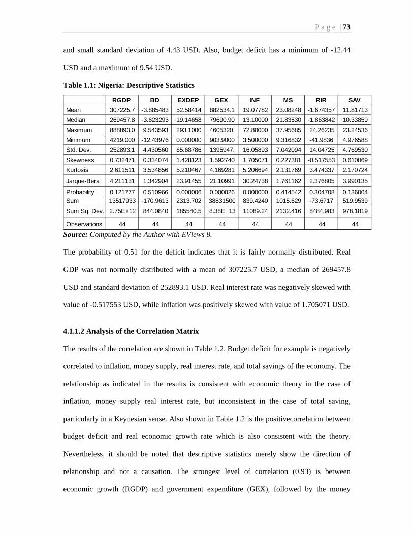
P a g e | 73

RGDP BD EXDEP GEX INF MS RIR SAV

Mean 307225.7 -3.885483 52.58414 882534.1 19.07782 23.08248 -1.674357 11.81713

Median 269457.8 -3.623293 19.14658 79690.90 13.10000 21.83530 -1.863842 10.33859

Maximum 888893.0 9.543593 293.1000 4605320. 72.80000 37.95685 24.26235 23.24536

Minimum 4219.000 -12.43976 0.000000 903.9000 3.500000 9.316832 -41.9836 4.976588

Std. Dev. 252893.1 4.430560 65.68786 1395947. 16.05893 7.042094 14.04725 4.769530

Skewness 0.732471 0.334074 1.428123 1.592740 1.705071 0.227381 -0.517553 0.610069

Kurtosis 2.611511 3.534856 5.210467 4.169281 5.206694 2.131769 3.474337 2.170724

Jarque-Bera 4.211131 1.342904 23.91455 21.10991 30.24738 1.761162 2.376805 3.990135

Probability 0.121777 0.510966 0.000006 0.000026 0.000000 0.414542 0.304708 0.136004 Sum 13517933 -170.9613 2313.702 38831500 839.4240 1015.629 -73.6717 519.9539

Sum Sq. Dev. 2.75E+12 844.0840 185540.5 8.38E+13 11089.24 2132.416 8484.983 978.1819

Observations 44 44 44 44 44 44 44 44

and small standard deviation of 4.43 USD. Also, budget deficit has a minimum of -12.44

USD and a maximum of 9.54 USD.

Table 1.1: Nigeria: Descriptive Statistics

Source: Computed by the Author with EViews 8. The probability of 0.51 for the deficit indicates that it is fairly normally distributed. Real

GDP was not normally distributed with a mean of 307225.7 USD, a median of 269457.8

USD and standard deviation of 252893.1 USD. Real interest rate was negatively skewed with

value of -0.517553 USD, while inflation was positively skewed with value of 1.705071 USD.

4.1.1.2 Analysis of the Correlation Matrix

The results of the correlation are shown in Table 1.2. Budget deficit for example is negatively

correlated to inflation, money supply, real interest rate, and total savings of the economy. The

relationship as indicated in the results is consistent with economic theory in the case of

inflation, money supply real interest rate, but inconsistent in the case of total saving,

particularly in a Keynesian sense. Also shown in Table 1.2 is the positivecorrelation between

budget deficit and real economic growth rate which is also consistent with the theory.

Nevertheless, it should be noted that descriptive statistics merely show the direction of

relationship and not a causation. The strongest level of correlation (0.93) is between

economic growth (RGDP) and government expenditure (GEX), followed by the money

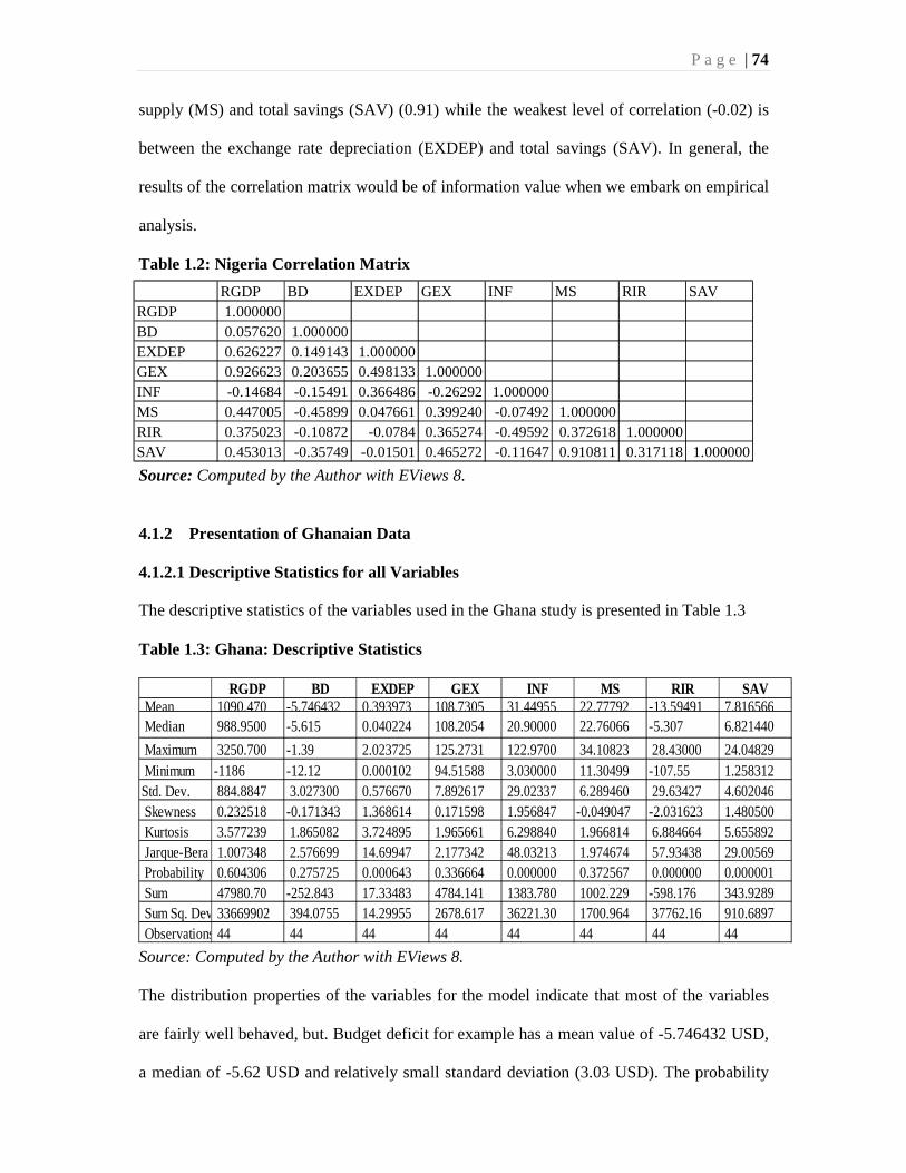
P a g e | 74

RGDP BD EXDEP GEX INF MS RIR SAVRGDP 1.000000BD 0.057620 1.000000EXDEP 0.626227 0.149143 1.000000GEX 0.926623 0.203655 0.498133 1.000000INF -0.14684 -0.15491 0.366486 -0.26292 1.000000MS 0.447005 -0.45899 0.047661 0.399240 -0.07492 1.000000RIR 0.375023 -0.10872 -0.0784 0.365274 -0.49592 0.372618 1.000000SAV 0.453013 -0.35749 -0.01501 0.465272 -0.11647 0.910811 0.317118 1.000000

RGDP BD EXDEP GEX INF MS RIR SAV Mean 1090.470 -5.746432 0.393973 108.7305 31.44955 22.77792 -13.59491 7.816566 Median 988.9500 -5.615 0.040224 108.2054 20.90000 22.76066 -5.307 6.821440

Maximum 3250.700 -1.39 2.023725 125.2731 122.9700 34.10823 28.43000 24.04829 Minimum -1186 -12.12 0.000102 94.51588 3.030000 11.30499 -107.55 1.258312Std. Dev. 884.8847 3.027300 0.576670 7.892617 29.02337 6.289460 29.63427 4.602046 Skewness 0.232518 -0.171343 1.368614 0.171598 1.956847 -0.049047 -2.031623 1.480500 Kurtosis 3.577239 1.865082 3.724895 1.965661 6.298840 1.966814 6.884664 5.655892 Jarque-Bera 1.007348 2.576699 14.69947 2.177342 48.03213 1.974674 57.93438 29.00569 Probability 0.604306 0.275725 0.000643 0.336664 0.000000 0.372567 0.000000 0.000001 Sum 47980.70 -252.843 17.33483 4784.141 1383.780 1002.229 -598.176 343.9289 Sum Sq. Dev. 33669902 394.0755 14.29955 2678.617 36221.30 1700.964 37762.16 910.6897 Observations 44 44 44 44 44 44 44 44

supply (MS) and total savings (SAV) (0.91) while the weakest level of correlation (-0.02) is

between the exchange rate depreciation (EXDEP) and total savings (SAV). In general, the

results of the correlation matrix would be of information value when we embark on empirical

analysis.

Table 1.2: Nigeria Correlation Matrix

Source: Computed by the Author with EViews 8.

4.1.2 Presentation of Ghanaian Data

4.1.2.1 Descriptive Statistics for all Variables

The descriptive statistics of the variables used in the Ghana study is presented in Table 1.3

Table 1.3: Ghana: Descriptive Statistics


The distribution properties of the variables for the model indicate that most of the variables

are fairly well behaved, but. Budget deficit for example has a mean value of -5.746432 USD,

a median of -5.62 USD and relatively small standard deviation (3.03 USD). The probability

P a g e | 75

RGDP BD EXDEP GEX INF MS RIR SAVRGDP 1.000000BD -0.210081 1.000000EXDEP 0.881085 -0.314326 1.000000GEX 0.699617 -0.142803 0.592907 1.000000INF -0.363742 0.113362 -0.376822 -0.377808 1.000000MS 0.465693 -0.37464 0.686128 0.511035 -0.255105 1.000000RIR 0.344141 -0.189115 0.271489 0.460002 -0.935488 0.171016 1.000000SAV 0.132245 -0.465212 0.298932 -0.249874 -0.210841 0.321991 0.142705 1.000000

of 0.28 for the deficit indicates that it is fairly normally distributed. Real GDP was normally

distributed with a mean 1090.47 USD, a median of 988.95 USD, Jacque-Bera probability

value of 2.58 USDand standard deviation of 884.89 USD. Real interest rate negatively

skewed at -2.03 USD while inflation was positively skewed with value 1.96 USD.

4.1.2.2 Analysis of the Correlation Matrix

Table 1.4 present the correlation matrix of the variables applied in this study. The highest

correlation (-0.94) is between inflation (INF) and real interest rate (RIR). This is consistent

with economic theory. The correlation coefficient of (-0.21) was registered between our

variable of interest budget deficit (BD) and real GDP. This not really a problem as the static

correlation is most times not a true reflection of the relationship between the variables when

dynamic models are specified. The weakest correlation (0.11) is between budget deficit (BD)

and inflation (INF).

Table 1.4: Ghana Correlation Matrix


4.2 Stationary (Unit Root) Tests Results

To examine the time series characteristics of the variables in the models, the Augmented

Dickey-Fuller (ADF) and Phillips-Perron (PP) stationarity (unit root) tests were conducted.

Essentially, both the ADF and PP tests are presented in table 1.5 below:

Table 1.5: Summary of ADF and PP Stationary (Unit Root) Tests for the Variables in

the Models, 1970 – 2013.

P a g e | 76

***Significant at 1%, **Significant at 5%, *Significant at 10% Source: Stationarity test results computed using EViews 8 Note: For both ADF and PP, the 5% critical values are given below the statistics in parentheses. Asterisk (**) shows no unit root at 5% critical value.

NIGERIA

Variables Augmented Dick-Fuller (ADF) Test Phillip-Perron (PP) Test At Level At First

Difference Order of

Cointegration

At Level At First Difference

Order of Cointegration

RIR -7.046315** (-3.518090)

- I(0) -3.518090** - I(0)

GEX - -4.561458* (-3.557759)

I(1) - -3.520787** I(1)

MS - -6.331609** (-3.520787)

I(1) - -3.520787** I(1)

INF - -6.587901** (-3.523623)

I(1) - -3.520787** I(1)

BD - -4.099735** (-3.520787)

I(1) -3.518090** - I(0)

RGDP - -5.238360** (-3.520787)

I(1) - -3.520787** I(1)

EXDEP -3.843817** (-3.518090)

- I(0) -3.518090** - I(0)

SAV - -6.001551** (-3.520787)

I(1) - -3.520787** I(1)

***Significant at 1%, **Significant at 5%, *Significant at 10%

GHANA Variables Augmented Dick-Fuller (ADF) Test Phillip-Perron (PP) Test





RIR - -11.30048** (-3.520787)

I(1) - -4.682621** (-3.518090)

I(1)

GEX -4.307310** (-3.518090)

- I(0) -4.261254** (-3.518090)

- I(0)

MS - -6.053898** (-3.520787)

I(1) - -6.057001** (-3.520787)

I(1)

INF -5.084804** (-3.518090)

- I(0) -5.029343** (-3.518090)

- I(0)

BD - -6.249993** (-3.520787)

I(1) - -7.440796** (-3.520787)

I(1)

RGDP - -9.619379** (-3.520787)

I(1) - -5.169553** (-3.518090)

I(1)

EXDEP - -5.463968** (-3.520787)

I(1) - -5.454011** (-3.520787)

I(1)

SAV -3.704077** (-3.518090)

- I(0) -3.682215** (-3.518090)

- I(0)

P a g e | 77

In Nigeria, the result of the unit root tests (ADF) shows that all the variables with the

exception of real interest rate and exchange rate depreciation failed the unit root test at 5%

level of significance in their level form. All variables, however, passed the test for

stationarity in their first difference. Similar results using Phillip-Perron (PP) test were carried

out, and the result also shows that all the variables with the exception of real interest rate,

budget deficit and exchange rate depreciation failed the unit root test at 5% level of

significance in their level form. All variables, however, passed the test for stationarity in their

first difference. In Ghana, both the ADF and PP test present identical results as all the

variables with the exception of government expenditure, inflation and savings failed the unit

root test at 5% level of significance in their level form. All variables passed the test for

stationarity in their first difference.

4.2.1 Lag Length/Bandwidth Selections

Appropriate lag length/Bandwidth was automatically chosen for the variables in the models

as informed by both Schwarz Information Criterion and Bartlett Kernel (See appendix for the

results).

4.3 Cointegration Tests

Having established the fact that some variables in the models are stationary at level I(0) and

others in first difference I(1), it is necessary to further examine if there exist a likelihood of a

long-run relationship amongst the variables. That is to ascertain if the variables are co-

integrated. Once this is done, it implies that although some of the variables exhibit random

walks, there is a stable long-run relationship amongst them and that the randomness will not

make them to diverge from their equilibrium relationship.

However, to do this, Engle-Granger two-step (EGTS) procedure on the variables that are

integrated to order one, that is I(1). The test involves first regressing these variables and

P a g e | 78

obtaining the residuals. Next, the residuals are tested for unit roots by applying ADF

framework. Once the results show a stationary process, it means that the variables are co-

integrated. Furthermore, this was done to know if the variables in the models have a

sustainable long-run relationship and also to avoid the problem of running a spurious

regression. The result for this test is reported in Table 1.6 below:

Table 1.6: Cointegration (Augmented Engle-Granger) Test Results

NIGERIA Variable ADF Test Statistic Test Critical Value at

5% Conclusion

RESID01 -5.936582 -2.931404 Stationary at level

GHANA

Variable ADF Test Statistic Test Critical Value at 5%

Conclusion

RESID01 -3.825501 -3.518090 Stationary at level Source: Author’s computation using EViews 8 The ADF tests on the residuals at level form confirmed that the calculated ADF statistics in

both Nigeria and Ghana are greater (in absolute terms) than the tabulated critical values at 5%

critical value. Thus, the null hypothesis of non-stationarity of the residuals is rejected, thus

concluding that there exist a stable long run relationship amongst them – though there might

be some deviations in the short-run.

4.4 Analysis of the SUR Models and Two-Stage Least Squares Estimation Results

To capture the three objectives of the study, a Seemingly Unrelated Regression (SUR) was

applied using both the Nigerian and Ghanaian data. The estimation of results for the SUR

model (equation 10, 11 and 12) are presented in Table 1.7 below. The equations represent

formulation of the hypotheses on the effects of budget deficits on (1.) interest rate, (2.)

inflation and (3) economic growth in both economies. However, the SUR estimation results

are presented in tables below:

P a g e | 79

Table 1.7: SUR Estimation Results Source: Author’s estimation using STATA 13.

Note: Asterisk (**) shows statistically significant at 5% level of significance. The t-Statistic is given below; the statistics in parentheses.

NIGERIA GHANA Variable RIR INF InRGDP RIR INF InRGDP GEX 1.91e-06

(1.25) -

- 0.7118853** (3.71)

-

BD -0.214025** (-3.42)

-1.457205** (-2.61)

-0.0161941** (-2.47)

-1.23363** (-2.71)

-1.1113837** (-3.08)

-0.0371651** (-3.57)

InRGDP - -2.236352 (-1.09)

- - -0.0064234 (-1.63)

-

InMS 12.40231 (1.66)

-11.90506 (-1.32)

- -19.1024** (-3.60)

-5.406567 (-0.28)

-

RIR - - 0.026369** (2.36)

-0.0079105** (-2.21)

INF -0.4221472** (-3.98)

-

0.0145521** (-3.38)

-0.9134943** (-19.35)

- -0.0140296** (-2.11)

EXDEP - 0.1373776** (3.37)

- - -5.146021** (-2.28)

-

InSAV -

- 0.5001784 (1.31)

-

- 0.0333115 (0.29)

Constant -34.47242 (-1.62)

69.77756** (2.90)

10.67361** (11.79)

-10.42766 (-0.51)

57.80081** (2.99)

7.013945** (26.68)

R2 0.78 0.85 0.82 0.92 0.74 0.70 Adjusted R2 0.76 0.83 0.81 0.90 0.73 0.69 Observation (Obs) 44 44 40 44 44 40 F-stat. (chi2) 34.31 16.85 12.90 496.03 5.60 15.54 P-Value 0.0000 0.0021 0.0118 0.0000 0.2308 0.0037 DW 1.376 1.431 1.576 1.423 1.631 1.391

P a g e | 80

P a g e | i

4.4.1 Analysis of the SUR Estimation based on Economic Criteria

The estimation results for the Seemingly Unrelated Regression (SUR) equations are presented in

Table 1.7above. The equations represent formulation of the hypotheses that budget deficits exert

effects on interest rate (first study objective), inflation (second objective), and economic growth

(third objective) in Nigeria and Ghana.

The result obtained from the estimation exercise are fairly robust and satisfactory, such that the

variables in the estimation models conformed largely to a priori expectations in terms of

statistical significance. However, as indicated in the SUR equations results above, some

estimated coefficients are consistent with a priori expectations, while others are not. Focusing

our major interest on our core variable which is budget deficit, it is of great interest to note that

the coefficients of the variables in three equations (as shown in Table 1.7) maintain negative

signs in line with our a priori expectations. This suggests that the relationship between budget

deficit; interest rate, inflation and economic growth from the linear-log and log-log form of the

model(s)in Nigeria and Ghana are respectively negative. The t-statistics, that is, the variables in

parentheses in the Table (1.7) confirm that the coefficient of budget deficit is statistically

significant at 5.0 percent. Thus, we can safely reject the null hypotheses that budget deficits do

not have significant effects on interest rate, inflation and economic growth in Nigeria and Ghana.

Furthermore, the coefficients of budget deficit is negatively related to interest rate (RIR) in the

first model; inflation (INF) in the second model, and economic growth (RGDP) in the third

model, but allare statistically significant. This further suggests that, if budget deficit increases by

one percent, the interest rate, inflation and economic growth will decrease by about 0.21%,

2.61%, and 2.47% in Nigeria respectively. Similarly, in Ghana, if budget deficit increases by one

percent, the interest rate, inflation and economic growth will decrease by about 1.23%, 1.11%,

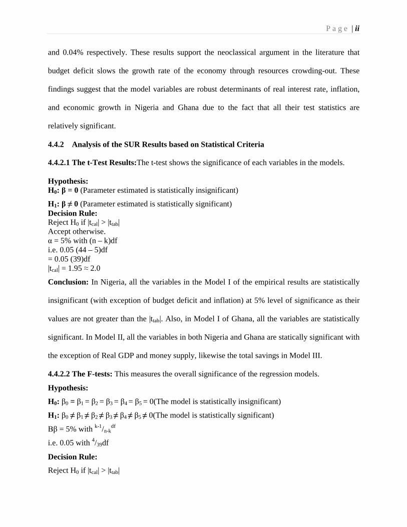
P a g e | ii

and 0.04% respectively. These results support the neoclassical argument in the literature that

budget deficit slows the growth rate of the economy through resources crowding-out. These

findings suggest that the model variables are robust determinants of real interest rate, inflation,

and economic growth in Nigeria and Ghana due to the fact that all their test statistics are

relatively significant.

4.4.2 Analysis of the SUR Results based on Statistical Criteria

4.4.2.1 The t-Test Results:The t-test shows the significance of each variables in the models. Hypothesis: H0: β = 0 (Parameter estimated is statistically insignificant)

H1: β ≠ 0 (Parameter estimated is statistically significant) Decision Rule: Reject H0 if |tcal| > |ttab| Accept otherwise. α = 5% with (n – k)df i.e. 0.05 (44 – 5)df = 0.05 (39)df |tcal| = 1.95 ≈ 2.0

Conclusion: In Nigeria, all the variables in the Model I of the empirical results are statistically

insignificant (with exception of budget deficit and inflation) at 5% level of significance as their

values are not greater than the |ttab|. Also, in Model I of Ghana, all the variables are statistically

significant. In Model II, all the variables in both Nigeria and Ghana are statically significant with

the exception of Real GDP and money supply, likewise the total savings in Model III.

4.4.2.2 The F-tests: This measures the overall significance of the regression models.

Hypothesis:

H0: β0 = β1 = β2 = β3 = β4 = β5 = 0(The model is statistically insignificant)

H1: β0 ≠ β1 ≠ β2 ≠ β3 ≠ β4 ≠ β5 ≠ 0(The model is statistically significant)

Ββ = 5% with k-1/n-kdf

i.e. 0.05 with 4/39df

Decision Rule:

Reject H0 if |tcal| > |ttab|

P a g e | iii

Accept otherwise

F-cal: the values of F-cal in the three (3) models in both economies are all greater than F-tab (see Table 1.7). Where; F-tab = 2.69 Therefore, since F-cal > F-tab in all the models in Nigeria and Ghana, we reject H0 and conclude that the models are statistically significant at 5% level of significance. 4.4.2.3 The Coefficient of Determinations (R2):

In the Table 1.7, the values of R2 in the three (3) models in Nigeria and Ghana hovers between

0.70 and 0.92. However, the R2explains the extent at which the respective dependent variables

(real interest rate, inflation and economic growth respectively) caused the variations in all the

explanatory variables in the respective models. This further suggests that the explanatory

variables explain about specific percentages of the total variations in real interest rate, inflation

and economic growth in the models in both economies respectively.

4.4.3 Analysis of the SUR Estimation based on Econometric Criteria

4.4.3.1 Autocorrelation

The Durbin-Watson (DW) test statistic was employed to check for serial correlation in the

model. From the empirical results presented in Table 1.7, DW ranges from the minimum 1.376

to maximum of 1.631 in the models of the two economies. n = 44; k = 5 (on the average,

excluding the intercept) and from the DW table; dL = 1.336and dU = 1.720 at 0.05 level.

Hypothesis:

H0: No positive autocorrelation

H0: No negative autocorrelation

H1: There is autocorrelation

Decision Rule:

P a g e | iv

Since dL<1.376 < - ... < 1.631< dU, there is inconclusive evidence regarding the presence or

absence of positive first order serial correlation.

4.4.3.2 Other Diagnostic Tests Table 1.8: Other Diagnostic Tests

Source: Author’s estimation using EViews 8 The result of residuals generated the estimated equation was found to be normally distributed for

both Nigeria and Ghana. No serial correlation and heteroscedasticity was observed in the

equation, implying that the estimates are reliable, and result can be relied on for policy

recommendation and formulation.

4.4.3.3 Functional Form Specification (Ramsey Reset) Test

This test is conducted to check whether the models in this study are correctly specified or not.

Here, the F-distribution was used.

NIGERIA

Test Type Statistic Value Probability Remarks Normality Jarqua

Bera 1.684908 0.430654 Normally distributed

residuals Serial Correlation (LM)

F-statistic 6.913589 0.0029 No serial correlation

Heteroscedasticity ( Harvey )

F-statistic 0.821468 0.6475 No heteroscedasticity

GHANA

Test Type Statistic Value Probability Remarks Normality Jarqua

Bera 2.886401 0.236171 Normally distributed

residuals Serial Correlation (LM)

F-statistic 1.136370 0.3319 No serial correlation

Heteroscedasticity (Harvey)

F-statistic 1.339767 0.2464 No heteroscedasticity

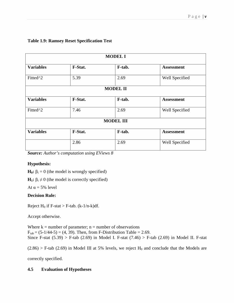
P a g e | v

Table 1.9: Ramsey Reset Specification Test

Source: Author’s computation using EViews 8 Hypothesis:

H0: βi = 0 (the model is wrongly specified)

H1: βi ≠ 0 (the model is correctly specified)

Αt α = 5% level

Decision Rule:

Reject H0 if F-stat > F-tab. (k-1/n-k)df.

Accept otherwise.

Where k = number of parameter; n = number of observations Ftab = (5-1/44-5) = (4, 39). Then, from F-Distribution Table = 2.69. Since F-stat (5.39) > F-tab (2.69) in Model I. F-stat (7.46) > F-tab (2.69) in Model II. F-stat

(2.86) > F-tab (2.69) in Model III at 5% levels, we reject H0 and conclude that the Models are

correctly specified.

4.5 Evaluation of Hypotheses

MODEL I

Variables F-Stat. F-tab. Assessment

Fitted^2 5.39 2.69 Well Specified

MODEL II


Fitted^2 7.46 2.69 Well Specified

MODEL III


2.86 2.69 Well Specified

P a g e | vi

The study hypotheses stated in Section 1.5 are evaluated as follow:

H01: Budget deficitshas noeffects on interest rate in Nigeria and Ghana.

Decision:

The t-statistic of the slope of the budget deficit on interest rate is -3.42 and -2.71 in Nigeria and

Ghana respectively, hence statistically significant at 5% (α > 1.95 ≈ 2). We reject the null

hypothesis that budget deficits has no effects on interest rate, thereby concluding that there exists

significant negative effect of budget deficits on interest rate in Nigeria and Ghana.

H02: Budget deficitshas noeffects on inflation in Nigeria andGhana

Decision:

The t-value of the slope of the budget deficit on inflation is -2.61 in Nigeria, and -3.08 in Ghana;

hence statistically significant at 5% (α > 1.95 ≈ 2). We reject the null hypothesis that budget

deficits has no effects on inflation, thereby concluding that there exists significant negative effect

of budget deficits on inflation in Nigeria and Ghana.

H03: Budget deficits has no effects on economic growth in Nigeria and Ghana.

Decision:

The t-value of the slope of the budget deficit on economic growth is -2.47 and -3.57 in Nigeria

and Ghana respectively, hence statistically significant at 5% (α > 1.95 ≈ 2). We reject the null

hypothesis that budget deficit has no effects on economic growth in both economies, thereby

concluding that there exists significant negative effect of budget deficits on interest rate in

Nigeria and Ghana. However, these findings support the neoclassical argument in the literature

that budget deficit slows the growth rate of the economy through resources crowding-out. The

P a g e | vii

policy implication of the findings is that the selected macroeconomic variables are negatively

affected by budget deficits in both economies of Nigeria and Ghana.

P a g e | viii

CHAPTER FIVE

SUMMARY, CONCLUSION, AND POLICY RECOMMENDATIONS

5.1 Summary of Findings

The study was carried out to empirically address three research questions on the fiscal deficits in

Nigeria and Ghana for the period from 1970 to 2013 inclusive. The motivation and justification

behind the study and selection of the economies of Nigeria and Ghana were as a result of:first,

the centrality of role of fiscal imbalances in determining the economic growth and stability in

both economies. Second, the similarities in socio-economic and political structures in both

economies. Hence, the study broadly aimed to test for the effects of budget deficits on interest

rates, inflation and economic growth in Nigeria and Ghana.

After testing for these effects of budget deficits on the selected macroeconomic variables in both

economies, the empirical results have shown that there exists negative and statistically

significant effects of budget deficits on interest rate, inflation and economic growth in Nigeria

and Ghana.

5.2 Policy Implications of Findings The results from the study clearly show that budget deficits in Nigeria and Ghana are responsible

for macroeconomic imbalances. An ever rising inflation and interest rates are not desirable and

they could be instrumental for disaster if they reach unsustainable levels. Inflation and interest

rates are unsustainable if they cannot be controlled and their effects are not consistent with

adequate growth, price stability and the countries’ ability to service fully their external debt

P a g e | ix

obligations, (IMF, 1995). Similarly, high interest rates crowd out the private sector and thus

negatively affect national savings and investment. It is therefore necessary for the governments

of Nigeria and Ghana to reduce the size of the budget deficits to a level that will not affect other

macroeconomic variables through fiscal consolidation and boosting domestic production.

Fiscal Consolidations in Nigeria and Ghana

Fiscal consolidation is a policy aimed at reducing government deficits and debt accumulation.

For Nigeria and Ghana the policy should focus on both short term and long term measures. In the

short term the government should aim at gradually reducing the budget deficit by raising

domestic revenue mobilization. In Nigeria and Ghana, revenue from tax (tax to GDP ratio) has

stagnated between 11 and 13 percent over the years yet government spending have continued to

grow (NBS, 2013; BoG, 2014).

5.3 Policy Recommendations

Financing of the growing expenditure has therefore been through foreign aid and government

borrowing both externally and internally; these as noted, have negative consequences. In order to

mitigate the above consequences, governments should institute actions that increase its revenue

collections. Such actions should aim at increasing economies’ tax revenue collections by

adopting efficient and effective methods of tax collections. Such measures include but are not

limited to the following:

i. Reducing the size of the informal sector which has proved hard to tax as this will improve

the revenue collection in the economies that can be used to finance budget deficits rather

than depending on external borrowing for financing of fiscal deficits. Similarly, reducing

the number of unproductive tax exemptions as well as combating tax evasion in the

economies will equally improve the revenue base of the governments.

P a g e | x

ii. Interest rates should be further reduced through appropriate policy and macroeconomic

environments to ensure credit availability and accessibility to the private sectors in both

economies. Furthermore, there is need to support growth in the real sectors of the

economy by encouraging investors to have access to investible funds from banks through

lowering of interest rate.

iii. Appropriate policy to ensure high levels of financial deepening should be pursued in both

economies as there exist the positive nexus between the level of financial deepening and

economic growth in both economies.

iv. Exchange rate depreciation should be discouraged in both economies as it has negative

consequences on growth in Nigeria and Ghana.

v. Appropriate policies should be pursed with vigour by the monetary authorities in both

economies to curtail inflation through suitable money supply. However, the regional

blocks at which the economies of Nigeria and Ghana belong should be mindful of

uniformed policy adoption across country members as this has implication on inflation.

vi. On the expenditure side, government should reduce its overall recurrent expenditure bill,

this could be done by revising the administrative structures created under its

decentralization plan. Also, governments of both economies should maintain the number

of states and local autonomies it had created as rapid growth in the number of districts,

states and local autonomies have contributed to increase in administrative costs which

worsens the budget imbalances.

vii. The economies should pursue policies that will boost production of goods for both

domestic consumption and exports in the long run through a combination of import

P a g e | xi

substitution and export promotion strategies as this will have a positive improvement on

the countries exchange rate, reduce inflation and thus lead to growth.

viii. Finally, the government of Nigeria and Ghana should be mindful of the sources of

financing the budget deficits so as to effectively manage the economic fluctuations and

increase activities in the real sector. Similarly, there is need to entrench fiscal discipline

in government operations at all levels that will ensure management of public finances,

improve budgetary processes, including openness in the budget preparation, execution

and reporting is been advocated.

5.4 Conclusion

The review of the study has shown that while vast growing volumes of research were being

carried out in the developed economies, little attention has been paid to the issue of how the

fiscal deficits affect interest rate, inflation, and economic growth in both economies. Based on

this empirical analysis, appropriate policies can then be drawn given insight to how budget

deficit can perform its roles without necessarily leading to inflation.

In order to achieve high and sustained long-run economic growth when budget deficit is used as

fiscal policy instrument, then, monetary policy, industrial policy and commercial policy must be

strengthened to act as checks and balances in Nigeria and Ghana. Relevant measures to enhance

policy coordination among various arms of government should be put in place. Most especially,

monetary policy should be made to complement fiscal policy measures. Also, fiscal discipline

should be strongly adhered to at every level of government. Furthermore, since inflation has been

established as monetary phenomenon in both Nigerian and Ghanaian economies; for budget

deficit to be effective, some fundamental changes in the productive base of the economy need be

made.

P a g e | xii

REFERENCES

Abel, A. B., & Bernanke, B. S. (2001). Macroeconomics (4thed.). New York: Addison Wesley

Longman, Inc.

Ackah, C. G, Aryeetey, E. B, & Aryeetey, E. (2009). The Impact of Global Economic Crisis on

Ghana. Labour Institute and Labour Research, Discussion Series Paper 5. Retrieved

from: http://www.ghanatuc.org/The-Effects-of-the-Global-Economic-and-Financial-

Crisis-on-the-Ghanaian-Economy-and-Labour-Market.pdf.

African Economic Outlook (2014). Ghana Overview 2014. Retrieved from:

http://www.africaneconomicoutlook.org/fileadmin/uploads/aeo/2014/PDF/CN_Long_EN

/Ghana_ENG.pdf.

African Economic Outlook (AEO) (2015). Regional Development and Spatial Inclusion.

Retrieved from:

http://www.africaneconomicoutlook.org/fileadmin/uploads/aeo/2015/PDF_Chapters/Over

view_AEO2015_EN-web.pdf

African Economic Outlook (AEO) (2013). Structural Transformation of Natural Resources.

Retrieved

from:http://www.undp.org/content/dam/rba/docs/Reports/African%20Economic%20Outl

ook%202013%20En.pdf

P a g e | xiii

Aisen, A., & Hauner, D. (2008). Budget Deficits and Interest Rates: A Fresh Perspective, IMF

Working Paper, Fiscal Affairs Department, International Monetary Fund, WP/08/42.

Akinboade, O. A. (2004). The Relationship between Budget Deficit and Interest Rates in South

Africa: Some Econometric Results. Development Southern Africa, Volume 21, Issue 2.

Akosah, N. K. (2013). Threshold Effect of Budget Deficits on Economic Growth in Ghana: An

Empirical Analysis. Bank of Ghana working Paper. 1-24

Andrew, M. (1991). Negotiating theSingleEuropeanAct: National Interestsand Conventional

Statecraft inthe European Community. World Peace Foundation and the Massachusetts

Institute of Technology (International Organisation), 45(1), 1 – 38.

Angrist, J. D., & Imbens, G. W. (1995). Two-stage least squares estimation of average causal

effects in models with variable treatment intensity. Journal of the American Statistical

Association, 90(430), 431-442.

Antwi, S. Z. X. (2009). Impact of Financial Reforms on the Banking System in Ghana.

International Business & Economics Research Journal, 8(3), 38 – 52.

Antwi, S. Z. X., & Mills, E. F. E. (2013). Consequential Effects of Budget Deficit on Economic

Growth: Empirical Evidence from Ghana. International Journal of Economics and

Finance, 5(3), 28 – 43.

Anyanwu, J. C. (1997). “Fiscal Relations among the Various Tiers of Government in Nigeria”,

Fiscal Federalism and Nigeria’s Economic development: Ibadan. The Nigerian

Economic Society.

Anyanwu, J. C. (1997). Nigerian Public Finance (1sted.). Onitsha: Joane Publishers.

Arestis, P. & Sawyer, M. (2006). The Inter-temporal Budget Constraint and the Sustainability of

Budget Deficits. Leeds: University of Leeds.

P a g e | xiv

Ariyo, A. & Raheen, M. I. (1991). Effects of Fiscal Deficits on Some Macroeconomic

Aggregates in Nigeria cited in Tchokote (2004). Macroeconomics of Fiscal Deficits in

Cameroun, Doctoral Dissertation, University of Ibadan.

Awe, A. A & Funlayo A. K. (2014). The Short and Long-Run Implications of Budget Deficit on

Economic Growth in Nigeria. Canadian Social Science, 10(5), 201-205.

Bakare, I.A.O., Adesanya, O.A and Bolarinwa, S.A. (2014). Empirical investigation between

budget deficit, inflation and money supply in Nigeria. European Journal of Business and

Social Sciences, 2(12), 120-134.

Baltagi, B. H., (2008). Econometric Analysis of Panel Data (4thed.). USA: John Wiley & Sons.

Bank of Ghana (2005).The HIPC Initiative and External Debt: An Empirical Assessment and

Policy Challenges. Accra, Bank of Ghana Research Department. 2-4.

Bank of Ghana (2007). Bank of Ghana Monetary Policy Report. Vol. 1, No. 6/2007. Accra, Bank

of Ghana Research Department. 4.

Bank of Ghana. (2007). Bank of Ghana Monetary Policy Report. Vol. 1, No. 6/2007. Accra,

Bank of Ghana Research Department. 2.

Barro, R. J. (1989). Rational-Expectations. National Review, 41(2).

Barro, R. J. (1990). Government Spending in A Simple Model of Endogenous

Growth, Journal of Political Economy, 98(3).

Barro, R. J. (1991). Economic Growth in A Cross Section of Countries, Quarterly

Journal of Economics, 106(6).

Barua, S. (2005). “An Examination of Revenue and Expenditure Causality in Bangladesh: 1974-

2004” World Bank Working Paper Series WP 0605 Dhaka, Bangladesh Bank Policy

Analysis Unit (PAU).

P a g e | xv

Bebi, H. (2000). Sustainability of Budget Deficits–A Case Study of Namibia (1991- 1999) Nepru

Working Paper No. 73, Windhoek, Namibian Economic Policy Research Unit.

Bernheim, B. D. (1989). A Neoclassical Perspective on Budget Deficits. Journal

of Economic Perspective, 3, 55 – 72.

Blanchard, O., & Johnson, D. R. (2012). Macroeconomics (6thed.). New York: Pearson

Publication, Inc.

Bonga-Bonga, L (2011). “Budget deficit and long-term interest rates in South Africa”.

University of Johannesburg, Department of Economics and Econometrics, Auckland

Park, 2006, South Africa.

Brownbridge, M. & Tumusiime-Mutebile, E. (2007). Aid and Fiscal Deficits: Lessons from

Uganda on the Implications for Macroeconomic Management and Fiscal Sustainability.

Development Policy Review, 25(2), 193 – 213.

Bullock, J. G.,Green, D. P., & Ha, S. E. (2010). Yes, But What’s the Mechanism? (Don’t Expect

an Easy Answer). Journal of Personality and Social Psychology98 (4): 550–558.

Buscemi, A. & Yallwe, A. H. (2012). Fiscal Deficit, National Saving and Sustainability of

Economic Growth in Emerging Economies: A Dynamic GMM Panel Data Approach.

International Journal of Economics and Financial Issues, 2(2), 2146 – 4138.

Catão, L. A.V. & Terrones M. E, (2005). Fiscal Deficits and Inflation. Journal of Monetary

Economics, 52(7), 529 – 554.

Darrat, A. F. (1985). Inflation and Federal Budget Deficits: Some Empirical Results. Public

Finance Quarterly, 13(8), 206-215.

Darrat, A. F. (2000). Are Budget Deficits Inflationary? A Reconsideration of the Evidence.

Applied Economics, 7(10), 633-36.

P a g e | xvi

Daumont, R., Le Gall, F., & Leroux, F. (2004). Banking in Sub-Saharan Africa: What went

wrong? IMF Working Paper. WP/04/55.

Dernberg, T.F. (1988). Macroeconomics Concepts Theories and Policies. USA: McGraw Hill

Publishing Company.

Dickey, D. A. & Fuller, W. A. (1979). Distribution of the Estimators for Autoregressive Time

Series with a Unit Root. Journal of the American Statistical Association, 74(5), 427 –

431.

Dockery, E., & Ezeabasili, V. N. (2012). The Relationship between Fiscal Deficits and Inflation:

Econometric Evidence for Nigeria. Economics and Finance Review, 2(7), 17 – 30.

Dwyer, G. P. (1982). Inflation and Government Deficits. Economic Inquiry,XX(3), 315 – 329.

Easterly, W. & Schmidt-Hebbel, K. (1991). The Macroeconomics of Public Sector Deficits: A

Synthesis. The World Bank Working Paper Series. No. 775.

Easterly, W., Schmidt-Hebbel K. (1993). Fiscal Deficits and Macroeconomic Performance in

Developing Countries. World Bank Research Observer, 8(2) 211 – 237.

Eisner, E. J. (1989). Budget Deficits: Rhetoric and Reality. Journal of Economic

Perspectives, 3(7), 23 – 43.

Engle, R. F., & Granger, C. W. J. (1987). Cointegration and Error Correction: Representation,

Estimation and Testing. Econometric, 55 (2), 251-276.

Ezeabasili V. N., Mojekwu, J. N., & Herbert, W. E. (2012). An Empirical Analysis of Fiscal

Deficits and Inflation in Nigeria. International Business and Management, 4(1), 105 –

120.

Ezeabasili, V. N., & Mojekwu, J. N. (2011). Analysis of Fiscal Deficits and Interest Rates in

Nigeria. Journal of Economics and International Finance, 3(4), 236 – 245.

Gebhard, K., & Silika, P. (2006). Sustainability of Swiss Fiscal Policy. CESIFO Working Paper

1689(1), Switzerland, University of St. Gallen. Retrieved from http://www.cesifo-

P a g e | xvii

group.de/portal/page/portal/DocBase_Content/WP/WP-CESifo_Working_Papers/wp-ces

ifo-2006/wp-cesifo-2006-03/cesifo1_wp1689.pdf

Georgantopoulos, A.G., & Tsamis, A. D. (2011). The Macroeconomic Effects of Budget Deficits

in Greece: A VAR-VECM Approach. International Research Journal of Finance and

Economics, 79(2), 78 – 84.

Guess, G., & Koford, K. (1984). Inflation, Recession and Federal Budget Deficit

(or Blaming Economic Problems on A Statistical Mirage). Policy Sciences, 17(4), 21 – 37

Gujarati, D. N (2007). Basic Econometrics (4thed.). India: Tata McGraw –Hill.

Gupta, R. & Uwilingiye, J. (2009). Measuring the welfare cost of inflation in South Africa: a

reconsideration. South African Journal of Economic and Management Sciences, 12(2),

137 – 146.

Heng, T. K. (1997). Public Capital and Crowding In. The Singapore Economic

Review, 42(2), 32 – 42

Hyman, D. N. (1994). Economics (3rdEd.). Massachusetts: Richard D. Irwin Inc.

Institute of Economic Affairs (2008). Annual 2007 Economic Review and Outlook, Accra, 23 –

29.

Institute of Statistical, Social and Economic Research. (2007). State of the Ghanaian Economy in

2006. Accra-Legon: Wilco Publicity Services Ltd.

Johansen, S. (1991). Estimation and Hypothesis Testing of Cointegrating Vectors in Gaussian

vector Autoregressive Models. Econometrica, 59(3), 39 – 46.

Keating, J.W. (2000). Macroeconomic Modelling with Asymmetric Vector Autoregression.

Journal of Macroeconomics, 21(1).

P a g e | xviii

Keho, Y. (2010), Budget Deficits and Economic Growth: Causality Evidence and Policy

Implications for WAEMU Countries. European Journal of Economics, Finance and

Administrative Sciences, 18.

Larbi, D. A. (2012). The Long Term Impact of Budget Deficits on Economic Growth in

Ghana.Journal of Business Research, 6(2), 22 – 34.

Lin, H.Y., & Chu, H. P. (2013). Are fiscal deficits inflationary? Journal of International Money

and Finance, 32(3), 214 – 233.

Luporini, V. (1999). Sustainability of the Brazilian Fiscal Policy and Central Bank

Independence. Cedeplar Belo Horizonte, the Federal University of Minas Gerais.

Lwanga, M. M & Mawejje, J. (2014). Macroeconomic effects of Budget Deficits in Uganda: A

VAR-VECM Approach. Economic Policy Research Centre. Research Series No. 117.

MacKinnon, J. G. (1996). Numerical Distribution Functions for Unit Root and Cointegration

Test. Journal of Applied Econometrics, 11(3) 601 – 618.

Makochekanwa, A. (2008). The Impact of Budget Deficit on Inflation in Zimbabwe. University

of Pretoria, South Africa.

Mankiw, G. N. (2003). Macroeconomics (5thed.). New York: Worth Publishers Inc.

Mpia, M. N. & Ogrike J. (2014). Budget Deficits and Interest Rates in Nigeria: The VAR

Approach. African Social and Educational Journal, 3(1).

Mugume, A., & Obwona, M. (1998). Public Sector Deficit and Macroeconomic Performance in

Uganda”, Economic Policy Research Centre, EPRC Research Series No. 7.

Mukhtar, T., & Zakaria, M. (2008). Budget Deficits and Interest Rates: An Empirical Analysis

for Pakistan. Journal of Economic Cooperation. 29(2), 1 – 14.

P a g e | xix

Ndulu, B. & Connell, S. (2008). ‘Policy Plus: African Growth Performance’, in B. Ndulu, S.

O’Connell, R. Bates, P. Collier and C. Soludo (Ed) The Political Economy of Economic

Growth in Africa 1960 - 2000, Vol. 1. Cambridge, UK: CUP.

National Bureau of Statistics (NBS) (2013). Retrieved from:

http://www.nsb.gov.sc/statistics/national-accounts.

Newey, W. K., & West, K. D. (1994). Automatic Lag Selection in Covariance Matrix

Estimation. Review of Economic Studies, 61, 631 – 653.

Noula, A. G (2012). Fiscal Deficit and Nominal Interest Rate Determination in Cameroon: An

Application of the Loanable Funds Model. Global Advanced Research Journal of

Management and Business Studies 1(1), 006 – 029.

Obioma, E. C. (1998). Balance of Payments and Exchange Rate Management in Nigeria:

Empirical Evidence from the Monetary Approach. NCEMA Policy Analysis Series. 4 (2).

Odhiambo S. O., Momanyi G., Othuon L., & Aila F. O. (2013). The Relationship between Fiscal

Deficits and Economic Growth in Kenya: An Empirical Investigation. Greener Journal of

Social Sciences, 3 (6), 306 – 323.

Odionye, J. C & Uma, K. E. (2013). The Relationship between Budget Deficit and Interest Rate:

Evidence from Nigeria. European Journal of Business and Social Sciences, 2(1), 158 –

166.

Ogiogio, G. O. (1996). Exchange Rate Policy, Trade Policy Reform and the Balance of

Payments”. In Obadan, M. I. And M. A. Iyoha (Ed.). Macroeconomic Policy Analysis:

Tools, Techniques and Applications to Nigeria. National Center for Economic

Management and Administration.

Oladipo, S. O., & Akinbobola, T. O. (2011). Budget deficit and inflation in Nigeria: A Causal

Relationship. Journal of Emerging Trends in Economics and Management Sciences, 2(1),

1 – 8.

P a g e | xx

Omoka, P. C. & Oruka, L. I. (2010). Budget Deficits, Money Supply and Inflation in Nigeria.

European Journal of Economics, Finance and Administrative Sciences. 19(3).

Onuorah, A. C., & Ogomegbunam, O. A. (2013). Relationship between Macroeconomic

Variables and Budget Deficit. International Journal of Management Sciences, 1(10), 416

– 426.

Onwuoduokit, E (2005). Fiscal Deficit, Inflation and output in Nigeria: A Vector Error

Correction Model Approach. Journal of Economic and Financial Studies, 2 (1), 34 – 54

Orji, A., Akachukwu, S. U., & Ilori, E. A. (2014). Foreign Capital Inflows and Growth: An

Empirical Analysis of WAMZ Experience Using a Sure Model. International Journal of

Economics and Financial Issues, 4(4), 976 – 983.

Osuka, B. O.m & Achinihu, J. C. (2014). The Impact of Budget Deficits on Macro-Economic

Variables in the Nigerian Economy. International Journal for Innovation Education and

Research. 2(11), 164.

Oyeleke, J. O., & Adebisi, D. G. (2014). Econometric Analysis of Fiscal Deficit Sustainability of

Ghana. Journal of Economics and Sustainable Development, 5(28), 34 – 40.

Ozurumba, B. A. (2012). Fiscal Deficits and Inflation in Nigeria: The Causality Approach.

International Journal of Scientific & Technology Research, 1(8).

Phillips, P. C., & Perron, P. (1988). Testing for a Unit Root in Time Series Regression.

Biometrica, 75(2), 335 – 346.

Pomeyie, P. (2001). Macroeconomics: An Introductory Textbook. Accra: Wade Laurel co.

Sachs, J. D., & Larrain, F. B. (1993). Macroeconomics in the Global Economy. New Jersey:

Prentice-Hall Inc.

Saleh, A. S. (2003). Budget Deficit and Economic Performance: A Survey. University of

Wollongong, Economic Working Paper Series.

P a g e | xxi

Sowa, N. K. (1994). Fiscal Deficits, Output Growth and Inflation Targets in Ghana. World

Development, 22(3), 1105 – 1117.

State of the Ghanaian Economy (2009). Institute of Social and Statistical Research Report.

University of Ghana, Legon.

Turnovsky, S. J. (2000). Methods of Macroeconomic Dynamics (2nded.). Massachusetts: MIT

Press.

Udu, E. & Agu, G.A. (2000). Economics. Onitsha: African Fep Publishers Limited Book House

Trust.

Vamvoukas, G. A. (1998). Short and Long-Run Effects of Budget Deficits on Interest Rates.

Journal of Economic Literature, 50(1-2).

Vuyyuri, S., & Sesahiah, S. V., (2004). Budget Deficits and other Macroeconomic variables in

India. Applied Econometrics and International Development. AEEADE. 4-1(37).

Wetzel, D. L., & Roumeen, I. (1991). The Macroeconomics of Public Sector Deficits: The Case

of Ghana. Washington DC, World Bank. Retrieved from http://www-

wds.worldbank.org/servlet/WDSContentServer/WDSP/IB/1991/05/01/000009265_39610

01075 213/Rendered/PDF/multi_page.pdf

Wooldridge, J. M. (2006). Introductory Econometrics: A Modern Approach (5th Ed.). Retrieved

from: http://www.cengage.com

Wosowei, E. (2013). Fiscal Deficits and Macroeconomic Aggregates in Nigeria. Arabian

Journal of Business and Management Review, 2(9).

Xiomara, A. & Greenidge, K. (2003). Debt and Fiscal Sustainability in Barbados. Bridgetown,

Central Bank of Barbados.

P a g e | xxii

Yaya, K. (2010). Budget Deficit and Economic Growth: Causality Evidence and Policy

Implications for WAEMU Countries. European Journal of Economic, Finance and

Administration Sciences, Issue 18.

Yellen, J. L. (1989). Symposium on the Budget Deficit. Journal of Economic

Perspectives, 3(2).

APPENDIX DATA FOR THE REGRESSION (NIGERIA)

NIGERIA

YEAR BD RIR INF RGDP GEX MS EXDEP SAV 1970 -8.62 -29.2695 13.8 4,219.00 903.90 14.95 0.1 7.8 1971 2.58 5.576789 16 4,715.50 997.20 14.61 0.22 7.0 1972 -0.82 3.991658 3.5 4,892.80 1,463.60 14.69 0.2 7.9 1973 1.92 1.569258 5.4 5,310.00 1,529.20 14.67 0 8.4 1974 9.54 -25.6668 12.7 15,919.70 2,740.60 9.32 0.1 6.0

P a g e | xxiii

1975 -1.99 -13.9682 33.9 27,172.02 5,942.60 14.12 0.24 8.5 1976 -4.09 -6.86748 24.3 29,146.51 7,856.70 16.92 0.28 8.5 1977 -2.48 -4.2576 13.8 31,520.34 8,823.80 19.50 0.32 8.2 1978 -8.17 -6.28957 21.7 29,212.35 8,000.00 21.40 0.32 8.7 1979 3.48 -3.31985 11.7 29,947.99 7,406.70 21.88 0.32 9.9 1980 -3.98 -3.54742 10 31,546.76 14,968.50 23.89 0.28 11.6 1981 -8.19 -8.05542 20.8 205,222.06 11,413.70 30.4 0.34 13.78 1982 -12.44 5.355617 7.7 199,685.25 11,923.20 32.2 0.38 15.31 1983 -6.34 -3.58051 23.2 185,598.14 9,636.50 33.3 0.49 17.78 1984 -4.46 -5.4496 39.6 183,562.95 9,927.60 33.7 0.7 18.43 1985 -4.48 5.009445 5.5 201,036.27 13,041.10 32.8 0.83 18.44 1986 -11.94 10.6672 5.4 205,971.44 16,223.70 34.4 1.94 20.15 1987 -5.60 -24.2547 10.2 204,806.54 22,018.70 26.2 4.11 17.75 1988 -8.74 -3.05004 34.5 219,875.63 27,749.50 27.6 6.95 16.72 1989 -6.98 -16.3882 50.5 236,729.58 41,028.30 21.2 16.26 10.98 1990 -8.27 10.00194 7.4 267,549.99 60,268.20 19.8 18.03 11.08 1991 -11.45 7.590991 13 265,379.14 66,584.40 24.2 24.04 12.09 1992 -7.42 -23.9307 44.6 271,365.52 92,797.40 20.9 58.1 10.35 1993 -9.53 4.485998 57.2 274,833.29 191,228.90 24.2 114.7 12.43 1994 -7.81 -8.7724 57 275,450.56 160,893.20 25.6 174.4 12.05 1995 0.05 -41.9836 72.8 281,407.40 248,768.10 15.0 293.1 5.61 1996 1.19 -10.3085 29.3 293,745.38 337,217.60 12.8 19.07426 4.98 1997 -0.18 16.49756 8.5 302,022.48 428,215.20 14.7 19.2189 6.34 1998 -4.92 24.26235 10 310,890.05 487,113.40 18.0 19.87715 7.39 1999 -8.93 3.40836 6.6 312,183.48 947,690.00 19.7 53.7556 8.69 2000 -2.26 -10.25 6.9 329,178.74 701,059.40 19.2 58.24839 8.41 2001 -4.68 22.28285 18.9 356,994.26 1,018,025.60 26.9 70.58229 10.33 2002 -4.36 -12.7334 15.9 433,203.51 1,018,155.80 21.8 85.13346 8.57 2003 -2.39 8.560264 13.2 477,532.98 1,225,965.90 23.0 106.6806 7.73 2004 -1.51 -1.28127 15.8 527,576.04 1,426,200.00 18.7 126.6871 6.99 2005 -1.11 -1.51329 11.4 561,931.39 1,822,100.00 18.1 143.7826 9.04 2006 -0.55 -2.21439 8.5 595,821.61 1,938,002.50 20.5 148.3301 9.37 2007 -0.57 11.76407 6.566 634,251.14 2,450,896.70 24.8 155.7536 13.04 2008 -0.20 4.190484 15.148 672,202.55 3,240,820.00 33.0 93.64 16.95 2009 -3.27 23.7065 13.935 718,977.33 3,452,990.80 38.0 98.77 23.25 2010 -3.25 -7.23133 11.742 775,525.70 4,194,217.88 32.5 92.31 17.52 2011 -3.10 12.41647 10.333 834,000.83 4,299,155.10 32.4 89.91408 17.40 2012 -2.41 14.87001 11 888,893.00 4,605,319.72 27.10 87.3225 19.88 2013 -2.26 4.304165 9.5 800,925.60 4,194,218.88 27.30 127.87143 18.69 SOURCE: CBN Bulletin of various years, IMF, WDI 2014 DATA FOR THE REGRESSION (GHANA)

P a g e | xxiv

GHANA

YEAR BD RIR INF RGDP GEX MS EXDEP SAV 1970 -7.09 3.75 3.03 676 101.3677 18.90541 0.000102 12.78272

1971 -6.92 3 8.82 193 104.4751 18.9822 0.000103 9.642072

1972 -6.49 0.2 10.81 -292 94.51588 23.71457 0.000133 12.58791

1973 -4.18 -9.6 17.07 285 94.94459 22.66394 0.000116 14.08089

1974 -4.58 -11.3 18.75 1012 103.4763 21.5667 0.000115 9.57061

1975 -9.49 -19.8 29.82 -1186 99.0706 26.23718 0.000115 13.65512

1976 -9.34 -45.4 55.41 -354 100.3386 29.11235 0.000115 8.545556

1977 -5.64 -106.5 116.52 228 101.0561 27.28246 0.000115 10.0077

1978 -1.48 -57.85 73.09 848 101.3285 24.45824 0.000176 4.046489

1979 -1.42 -39.25 54.52 -251 99.92913 21.05489 0.000275 6.608319

1980 -1.39 -34.85 50.15 612.5 100.6884 18.55351 0.000275 4.935592

1981 -7.05 -101.25 117.86 644.2 100.5673 16.5651 0.000275 4.005453

1982 -10.79 -7.85 21.31 611.7 99.64373 17.1649 0.000275 3.733907

1983 -3.93 -107.55 122.97 590.6 100.4331 11.30499 0.000883 3.316707

1984 -4.57 -20.66 40 639.6 102.7266 11.81331 0.003597 4.150391

1985 -2.18 8.08 9.96 677 102.935 13.6185 0.005434 6.635012

1986 -2.36 -6.1 24.8 706.2 103.5596 13.51454 0.008916 5.802418

1987 -2.82 -18.26 39.75 747.6 106.5229 14.20509 0.015365 3.911053

1988 -1.75 -10.36 31.38 817.8 105.8787 14.74606 0.020224 5.417341

1989 -2.02 -2.05 25.26 855.4 107.6006 16.91699 0.026985 5.608394

1990 -1.5 -12.45 35.9 884 108.9724 14.14209 0.032616 5.471648

1991 -3.46 7.91 10.3 928.5 108.5613 15.56278 0.036763 7.317731

1992 -2.36 12.56 13.3 966.4 111.5417 20.52587 0.043685 1.258312

1993 -7.06 2.07 27.7 1011.5 116.1613 19.83546 0.064871 6.048895

1994 -8.81 1.93 34.2 1046.6 111.5039 22.51313 0.095568 12.45386

1995 -8.54 -27.13 70.8 1089 108.4302 21.64299 0.119914 11.5912

1996 -8.44 -9.1 32.7 1138.4 107.9806 20.59611 0.163547 13.21942

1997 -10.17 11.08 20.5 1197.9 120.5813 23.84196 0.204796 4.224961

1998 -9.85 28.43 15.7 1259.1 112.8568 22.85738 0.231166 10.25255

1999 -8.2 17.8 13.8 1318.1 117.5484 24.09283 0.266643 3.45211

2000 -8.54 4.6 40.5 1373.3 118.4439 28.16617 0.544919 5.554686

2001 -6.68 -5.227 21.3 1435 119.5798 31.44533 0.716305 7.0196

2002 -5.18 -9.37 17 1501.8 112.2567 34.10823 0.792417 7.443261

2003 -4.38 -7.01 31.3 1578.6 115.9291 31.04593 0.866764 7.007868

2004 -3.35 -8.443 16.4 1662.5 121.0637 32.72259 0.899495 7.313823

2005 -3.03 -5.387 13.9 1762.6 125.2731 32.11003 0.906279 3.72906

2006 -2.84 -4.707 10.9 1870.5 115.5376 23.26474 0.916452 6.098369

2007 -4.71 -2.84 12.7 1991.4 116.3044 25.71675 0.935248 3.803148

2008 -5.59 -3.026 18.1 2159.2 119.4555 27.46146 1.057858 1.996779

2009 -8.48 -3.349 16 2245.4 113.0106 28.24624 1.4088 7.659583

P a g e | xxv

2010 -5.82 -4.378 8.58 2425.2 116.4243 29.61919 1.421667 9.277813

2011 -8.25 -5.179 8.58 2789.1 105.5796 30.54902 1.659917 24.04829

2012 -12.12 8.08 8.84 3034.3 110.375 31.27799 1.841821 20.51003

2013 -9.993 -1.44 13.5 3250.7 119.7118 28.50346 2.023725 8.13225

SOURCE: Bank of Ghana Statistical Bulletin of various years, IMF, WEO, and WDI 2014 NIGERIA AUGMENTED DICKEY-FULLER (ADF) STATIONARITY TEST RES ULTS AS GENERATED FROM EVIEWS 8. AT LEVEL Null Hypothesis: BD has a unit root Exogenous: Constant, Linear Trend Lag Length: 0 (Automatic - based on SIC, maxlag=9)

t-Statistic Prob.* Augmented Dickey-Fuller test statistic -4.099735 0.0125

Test critical values: 1% level -4.186481 5% level -3.518090 10% level -3.189732 *MacKinnon (1996) one-sided p-values.

Augmented Dickey-Fuller Test Equation Dependent Variable: D(BD) Method: Least Squares Date: 08/26/15 Time: 23:14 Sample (adjusted): 1971 2013 Included observations: 43 after adjustments

Variable Coefficient Std. Error t-Statistic Prob. BD(-1) -0.579475 0.141345 -4.099735 0.0002

C -1.964088 1.394512 -1.408440 0.1667 @TREND("1970") -0.007341 0.050383 -0.145712 0.8849

R-squared 0.296392 Mean dependent var 0.147849

Adjusted R-squared 0.261211 S.D. dependent var 4.769469 S.E. of regression 4.099494 Akaike info criterion 5.726818 Sum squared resid 672.2339 Schwarz criterion 5.849693 Log likelihood -120.1266 Hannan-Quinn criter. 5.772130 F-statistic 8.424899 Durbin-Watson stat 1.878110 Prob(F-statistic) 0.000884

AT LEVEL Null Hypothesis: EXDEP has a unit root Exogenous: Constant, Linear Trend Lag Length: 0 (Automatic - based on SIC, maxlag=9)

t-Statistic Prob.*

P a g e | xxvi

Augmented Dickey-Fuller test statistic -3.843817 0.0235 Test critical values: 1% level -4.186481

5% level -3.518090 10% level -3.189732 *MacKinnon (1996) one-sided p-values.

Augmented Dickey-Fuller Test Equation Dependent Variable: D(EXDEP) Method: Least Squares Date: 08/26/15 Time: 23:15 Sample (adjusted): 1971 2013 Included observations: 43 after adjustments

Variable Coefficient Std. Error t-Statistic Prob. EXDEP(-1) -0.536569 0.139593 -3.843817 0.0004

C -12.75599 14.08480 -0.905656 0.3705 @TREND("1970") 1.954681 0.727263 2.687722 0.0104



AT 2ND DIFFERNCE Null Hypothesis: D(GEX,2) has a unit root Exogenous: Constant, Linear Trend Lag Length: 9 (Automatic - based on SIC, maxlag=9)



Augmented Dickey-Fuller Test Equation Dependent Variable: D(GEX,3) Method: Least Squares Date: 08/26/15 Time: 23:19 Sample (adjusted): 1982 2013 Included observations: 32 after adjustments

Variable Coefficient Std. Error t-Statistic Prob. D(GEX(-1),2) -16.83650 3.691036 -4.561458 0.0002

D(GEX(-1),3) 14.47944 3.500726 4.136126 0.0005 D(GEX(-2),3) 13.73803 3.176826 4.324453 0.0003 D(GEX(-3),3) 13.31895 2.960099 4.499494 0.0002

P a g e | xxvii

D(GEX(-4),3) 12.58975 2.759233 4.562772 0.0002 D(GEX(-5),3) 10.88162 2.480687 4.386533 0.0003 D(GEX(-6),3) 8.898648 2.138889 4.160407 0.0005 D(GEX(-7),3) 6.463939 1.740209 3.714462 0.0014 D(GEX(-8),3) 3.241325 1.189286 2.725437 0.0130 D(GEX(-9),3) 0.969074 0.462683 2.094468 0.0492

C -260759.7 102886.0 -2.534452 0.0197 @TREND("1970") 15286.39 4870.854 3.138340 0.0052

R-squared 0.971442 Mean dependent var -22067.15

Adjusted R-squared 0.955735 S.D. dependent var 563222.3 S.E. of regression 118497.3 Akaike info criterion 26.48316 Sum squared resid 2.81E+11 Schwarz criterion 27.03281 Log likelihood -411.7306 Hannan-Quinn criter. 26.66536 F-statistic 61.84846 Durbin-Watson stat 1.883371 Prob(F-statistic) 0.000000

1ST Difference Null Hypothesis: D(INF) has a unit root Exogenous: Constant, Linear Trend Lag Length: 1 (Automatic - based on SIC, maxlag=9)



Augmented Dickey-Fuller Test Equation Dependent Variable: D(INF,2) Method: Least Squares Date: 08/26/15 Time: 23:21 Sample (adjusted): 1973 2013 Included observations: 41 after adjustments

Variable Coefficient Std. Error t-Statistic Prob. D(INF(-1)) -1.443850 0.219167 -6.587901 0.0000

D(INF(-1),2) 0.371021 0.150925 2.458319 0.0188 C 2.793058 5.088512 0.548895 0.5864

@TREND("1970") -0.116825 0.196835 -0.593518 0.5564 R-squared 0.597405 Mean dependent var 0.268293


1ST DIFFERENCE

Null Hypothesis: D(MS) has a unit root Exogenous: Constant, Linear Trend

P a g e | xxviii

Lag Length: 0 (Automatic - based on SIC, maxlag=9) t-Statistic Prob.* Augmented Dickey-Fuller test statistic -6.331609 0.0000


Augmented Dickey-Fuller Test Equation Dependent Variable: D(MS,2) Method: Least Squares Date: 08/26/15 Time: 23:22 Sample (adjusted): 1972 2013 Included observations: 42 after adjustments

Variable Coefficient Std. Error t-Statistic Prob. D(MS(-1)) -1.013158 0.160016 -6.331609 0.0000

C 0.672960 1.371470 0.490685 0.6264 @TREND("1970") -0.016317 0.053577 -0.304550 0.7623



AT 1ST DIFFERENCE Null Hypothesis: D(RGDP) has a unit root Exogenous: Constant, Linear Trend Lag Length: 0 (Automatic - based on SIC, maxlag=9)



Augmented Dickey-Fuller Test Equation Dependent Variable: D(RGDP,2) Method: Least Squares Date: 08/26/15 Time: 23:23 Sample (adjusted): 1972 2013 Included observations: 42 after adjustments

Variable Coefficient Std. Error t-Statistic Prob. D(RGDP(-1)) -1.006525 0.192145 -5.238360 0.0000

C 5056.677 11836.99 0.427193 0.6716 @TREND("1970") 623.9178 504.8923 1.235744 0.2239

P a g e | xxix



AT 1ST DIFFERENCE Null Hypothesis: RIR has a unit root Exogenous: Constant, Linear Trend Lag Length: 0 (Automatic - based on SIC, maxlag=9)



Augmented Dickey-Fuller Test Equation Dependent Variable: D(RIR) Method: Least Squares Date: 08/26/15 Time: 23:24 Sample (adjusted): 1971 2013 Included observations: 43 after adjustments

Variable Coefficient Std. Error t-Statistic Prob. RIR(-1) -1.080467 0.153338 -7.046315 0.0000

C -9.267837 4.402235 -2.105257 0.0416 @TREND("1970") 0.367696 0.173198 2.122984 0.0400



AT 1ST DIFFERENCE Null Hypothesis: D(SAV) has a unit root Exogenous: Constant, Linear Trend Lag Length: 0 (Automatic - based on SIC, maxlag=9)


Test critical values: 1% level -4.192337 5% level -3.520787

P a g e | xxx

10% level -3.191277 *MacKinnon (1996) one-sided p-values.

Augmented Dickey-Fuller Test Equation Dependent Variable: D(SAV,2) Method: Least Squares Date: 08/26/15 Time: 23:25 Sample (adjusted): 1972 2013 Included observations: 42 after adjustments

Variable Coefficient Std. Error t-Statistic Prob. D(SAV(-1)) -0.964605 0.160726 -6.001551 0.0000

C 0.135832 0.816397 0.166379 0.8687 @TREND("1970") 0.005902 0.032035 0.184245 0.8548



GHANA PHILLIP-PERRON (PP) STATIONARITY TEST RESULTS AS GE NERATED FROM EVIEWS 8. AT LEVEL Null Hypothesis: BD has a unit root Exogenous: Constant, Linear Trend Bandwidth: 3 (Newey-West automatic) using Bartlett kernel

Adj. t-Stat Prob.* Phillips-Perron test statistic -4.250001 0.0085

Test critical values: 1% level -4.186481 5% level -3.518090 10% level -3.189732 *MacKinnon (1996) one-sided p-values. Residual variance (no correction) 15.63335

HAC corrected variance (Bartlett kernel) 18.27608

Phillips-Perron Test Equation Dependent Variable: D(BD) Method: Least Squares Date: 08/27/15 Time: 16:24 Sample (adjusted): 1971 2013 Included observations: 43 after adjustments

Variable Coefficient Std. Error t-Statistic Prob.

P a g e | xxxi

BD(-1) -0.579475 0.141345 -4.099735 0.0002 C -1.964088 1.394512 -1.408440 0.1667

@TREND("1970") -0.007341 0.050383 -0.145712 0.8849 R-squared 0.296392 Mean dependent var 0.147849


AT LEVEL Null Hypothesis: EXDEP has a unit root Exogenous: Constant, Linear Trend Bandwidth: 4 (Newey-West automatic) using Bartlett kernel




Phillips-Perron Test Equation Dependent Variable: D(EXDEP) Method: Least Squares Date: 08/27/15 Time: 16:27 Sample (adjusted): 1971 2013 Included observations: 43 after adjustments

Variable Coefficient Std. Error t-Statistic Prob. EXDEP(-1) -0.536569 0.139593 -3.843817 0.0004

C -12.75599 14.08480 -0.905656 0.3705 @TREND("1970") 1.954681 0.727263 2.687722 0.0104



P a g e | xxxii

AT FIRST DIFFERENCE Null Hypothesis: D(GEX) has a unit root Exogenous: Constant, Linear Trend Bandwidth: 2 (Newey-West automatic) using Bartlett kernel


Test critical values: 1% level -4.192337 5% level -3.520787 10% level -3.191277 *MacKinnon (1996) one-sided p-values. Residual variance (no correction) 3.66E+10

HAC corrected variance (Bartlett kernel) 4.82E+10

Phillips-Perron Test Equation Dependent Variable: D(GEX,2) Method: Least Squares Date: 08/27/15 Time: 16:28 Sample (adjusted): 1972 2013 Included observations: 42 after adjustments

Variable Coefficient Std. Error t-Statistic Prob. D(GEX(-1)) -1.187148 0.191448 -6.200890 0.0000

C -110891.6 68902.43 -1.609400 0.1156 @TREND("1970") 10277.64 3221.966 3.189868 0.0028



AT FIRST DIFFERENCE Null Hypothesis: D(INF) has a unit root Exogenous: Constant, Linear Trend Bandwidth: 18 (Newey-West automatic) using Bartlett kernel




P a g e | xxxiii

Phillips-Perron Test Equation Dependent Variable: D(INF,2) Method: Least Squares Date: 08/27/15 Time: 16:30 Sample (adjusted): 1972 2013 Included observations: 42 after adjustments

Variable Coefficient Std. Error t-Statistic Prob. D(INF(-1)) -1.054530 0.159877 -6.595897 0.0000

C 0.912014 5.142990 0.177332 0.8602 @TREND("1970") -0.047574 0.201282 -0.236355 0.8144



AT FIRST DIFFERENCE Null Hypothesis: D(MS) has a unit root Exogenous: Constant, Linear Trend Bandwidth: 0 (Newey-West automatic) using Bartlett kernel




Phillips-Perron Test Equation Dependent Variable: D(MS,2) Method: Least Squares Date: 08/27/15 Time: 16:31 Sample (adjusted): 1972 2013 Included observations: 42 after adjustments


C 0.672960 1.371470 0.490685 0.6264 @TREND("1970") -0.016317 0.053577 -0.304550 0.7623


Adjusted R-squared 0.481613 S.D. dependent var 5.840546

P a g e | xxxiv

S.E. of regression 4.205141 Akaike info criterion 5.779242 Sum squared resid 689.6453 Schwarz criterion 5.903361 Log likelihood -118.3641 Hannan-Quinn criter. 5.824737 F-statistic 20.04572 Durbin-Watson stat 1.998933 Prob(F-statistic) 0.000001

AT FIRST DIFFERENCE Null Hypothesis: D(RGDP) has a unit root Exogenous: Constant, Linear Trend Bandwidth: 5 (Newey-West automatic) using Bartlett kernel


Test critical values: 1% level -4.192337 5% level -3.520787 10% level -3.191277 *MacKinnon (1996) one-sided p-values. Residual variance (no correction) 1.23E+09

HAC corrected variance (Bartlett kernel) 9.61E+08

Phillips-Perron Test Equation Dependent Variable: D(RGDP,2) Method: Least Squares Date: 08/27/15 Time: 16:32 Sample (adjusted): 1972 2013 Included observations: 42 after adjustments


C 5056.677 11836.99 0.427193 0.6716 @TREND("1970") 623.9178 504.8923 1.235744 0.2239



AT LEVEL Null Hypothesis: RIR has a unit root Exogenous: Constant, Linear Trend Bandwidth: 6 (Newey-West automatic) using Bartlett kernel

Adj. t-Stat Prob.*

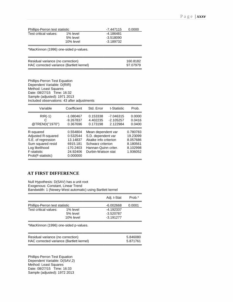
P a g e | xxxv

Phillips-Perron test statistic -7.447115 0.0000 Test critical values: 1% level -4.186481

5% level -3.518090 10% level -3.189732 *MacKinnon (1996) one-sided p-values. Residual variance (no correction) 160.8182


Phillips-Perron Test Equation Dependent Variable: D(RIR) Method: Least Squares Date: 08/27/15 Time: 16:32 Sample (adjusted): 1971 2013 Included observations: 43 after adjustments


C -9.267837 4.402235 -2.105257 0.0416 @TREND("1970") 0.367696 0.173198 2.122984 0.0400



AT FIRST DIFFERENCE Null Hypothesis: D(SAV) has a unit root Exogenous: Constant, Linear Trend Bandwidth: 1 (Newey-West automatic) using Bartlett kernel




Phillips-Perron Test Equation Dependent Variable: D(SAV,2) Method: Least Squares Date: 08/27/15 Time: 16:33 Sample (adjusted): 1972 2013

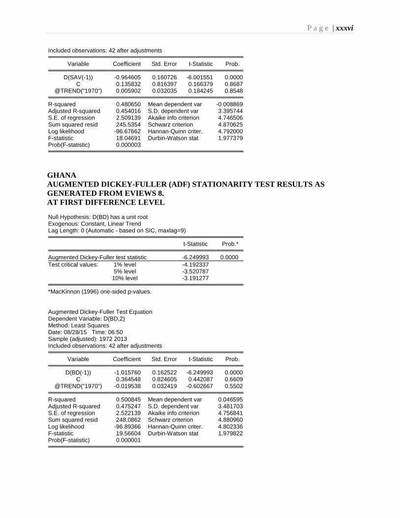
P a g e | xxxvi

Included observations: 42 after adjustments Variable Coefficient Std. Error t-Statistic Prob. D(SAV(-1)) -0.964605 0.160726 -6.001551 0.0000

C 0.135832 0.816397 0.166379 0.8687 @TREND("1970") 0.005902 0.032035 0.184245 0.8548



GHANA AUGMENTED DICKEY-FULLER (ADF) STATIONARITY TEST RES ULTS AS GENERATED FROM EVIEWS 8. AT FIRST DIFFERENCE LEVEL Null Hypothesis: D(BD) has a unit root Exogenous: Constant, Linear Trend Lag Length: 0 (Automatic - based on SIC, maxlag=9)



Augmented Dickey-Fuller Test Equation Dependent Variable: D(BD,2) Method: Least Squares Date: 08/28/15 Time: 06:50 Sample (adjusted): 1972 2013 Included observations: 42 after adjustments

Variable Coefficient Std. Error t-Statistic Prob. D(BD(-1)) -1.015760 0.162522 -6.249993 0.0000

C 0.364548 0.824605 0.442087 0.6609 @TREND("1970") -0.019538 0.032419 -0.602667 0.5502



P a g e | xxxvii

AT FIRST DIFFERENCE Null Hypothesis: D(EXDEP) has a unit root Exogenous: Constant, Linear Trend Lag Length: 0 (Automatic - based on SIC, maxlag=9)



Augmented Dickey-Fuller Test Equation Dependent Variable: D(EXDEP,2) Method: Least Squares Date: 08/28/15 Time: 06:54 Sample (adjusted): 1972 2013 Included observations: 42 after adjustments

Variable Coefficient Std. Error t-Statistic Prob. D(EXDEP(-1)) -0.869719 0.159174 -5.463968 0.0000

C -0.041446 0.023056 -1.797624 0.0800 @TREND("1970") 0.003730 0.001062 3.510195 0.0011


Adjusted R-squared 0.405642 S.D. dependent var 0.087428 S.E. of regression 0.067402 Akaike info criterion -2.487524 Sum squared resid 0.177180 Schwarz criterion -2.363404 Log likelihood 55.23799 Hannan-Quinn criter. -2.442029 F-statistic 14.99101 Durbin-Watson stat 2.026269 Prob(F-statistic) 0.000015

AT LEVEL Null Hypothesis: GEX has a unit root Exogenous: Constant, Linear Trend Lag Length: 0 (Automatic - based on SIC, maxlag=9)



Augmented Dickey-Fuller Test Equation Dependent Variable: D(GEX) Method: Least Squares Date: 08/28/15 Time: 06:55 Sample (adjusted): 1971 2013 Included observations: 43 after adjustments

P a g e | xxxviii

Variable Coefficient Std. Error t-Statistic Prob. GEX(-1) -0.624921 0.145084 -4.307310 0.0001

C 60.92844 14.16708 4.300704 0.0001 @TREND("1970") 0.331206 0.090124 3.675016 0.0007



AT LEVEL Null Hypothesis: INF has a unit root Exogenous: Constant, Linear Trend Lag Length: 0 (Automatic - based on SIC, maxlag=9)



Augmented Dickey-Fuller Test Equation Dependent Variable: D(INF) Method: Least Squares Date: 08/28/15 Time: 06:56 Sample (adjusted): 1971 2013 Included observations: 43 after adjustments

Variable Coefficient Std. Error t-Statistic Prob. INF(-1) -0.747009 0.146910 -5.084804 0.0000

C 40.67183 10.89788 3.732086 0.0006 @TREND("1970") -0.755611 0.342021 -2.209250 0.0329



AT FIRST DIFFERENCE Null Hypothesis: D(MS) has a unit root Exogenous: Constant, Linear Trend Lag Length: 0 (Automatic - based on SIC, maxlag=9)

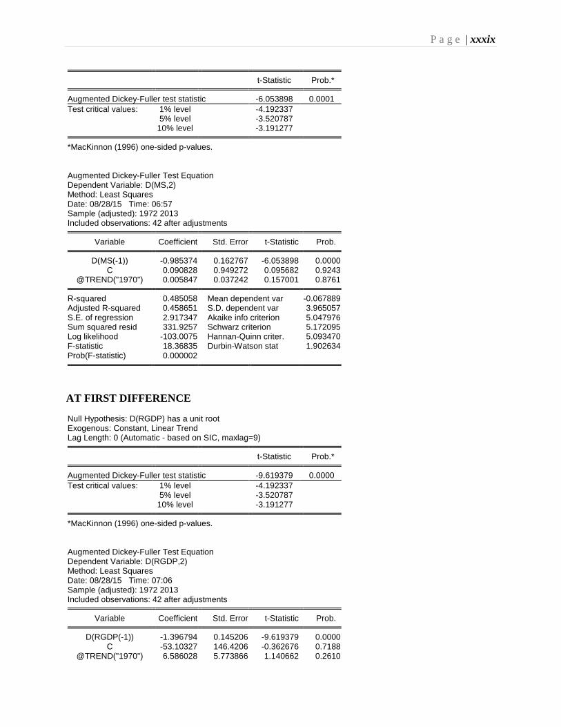
P a g e | xxxix



Augmented Dickey-Fuller Test Equation Dependent Variable: D(MS,2) Method: Least Squares Date: 08/28/15 Time: 06:57 Sample (adjusted): 1972 2013 Included observations: 42 after adjustments


C 0.090828 0.949272 0.095682 0.9243 @TREND("1970") 0.005847 0.037242 0.157001 0.8761



AT FIRST DIFFERENCE Null Hypothesis: D(RGDP) has a unit root Exogenous: Constant, Linear Trend Lag Length: 0 (Automatic - based on SIC, maxlag=9)



Augmented Dickey-Fuller Test Equation Dependent Variable: D(RGDP,2) Method: Least Squares Date: 08/28/15 Time: 07:06 Sample (adjusted): 1972 2013 Included observations: 42 after adjustments


C -53.10327 146.4206 -0.362676 0.7188 @TREND("1970") 6.586028 5.773866 1.140662 0.2610

P a g e | xl


Adjusted R-squared 0.688421 S.D. dependent var 804.2075 S.E. of regression 448.9024 Akaike info criterion 15.12024 Sum squared resid 7859023. Schwarz criterion 15.24436 Log likelihood -314.5250 Hannan-Quinn criter. 15.16573 F-statistic 46.29397 Durbin-Watson stat 2.396719 Prob(F-statistic) 0.000000

AT FIRST DIFFERENCE Null Hypothesis: D(RIR) has a unit root Exogenous: Constant, Linear Trend Lag Length: 0 (Automatic - based on SIC, maxlag=9)



Augmented Dickey-Fuller Test Equation Dependent Variable: D(RIR,2) Method: Least Squares Date: 08/28/15 Time: 07:20 Sample (adjusted): 1972 2013 Included observations: 42 after adjustments

Variable Coefficient Std. Error t-Statistic Prob. D(RIR(-1)) -1.533775 0.135727 -11.30048 0.0000

C -4.024335 9.085124 -0.442959 0.6602 @TREND("1970") 0.176607 0.355619 0.496618 0.6222



AT LEVEL Null Hypothesis: SAV has a unit root Exogenous: Constant, Linear Trend Lag Length: 0 (Automatic - based on SIC, maxlag=9)

t-Statistic Prob.*

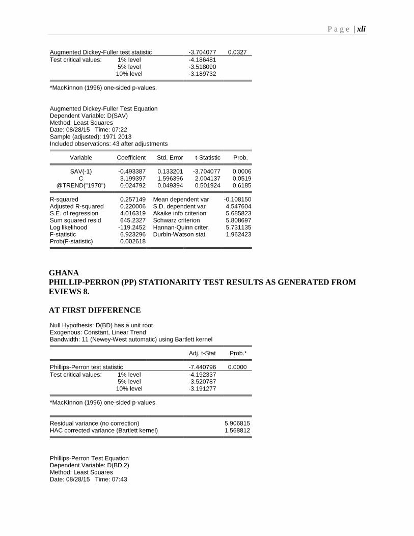
P a g e | xli

Augmented Dickey-Fuller test statistic -3.704077 0.0327 Test critical values: 1% level -4.186481

5% level -3.518090 10% level -3.189732 *MacKinnon (1996) one-sided p-values.

Augmented Dickey-Fuller Test Equation Dependent Variable: D(SAV) Method: Least Squares Date: 08/28/15 Time: 07:22 Sample (adjusted): 1971 2013 Included observations: 43 after adjustments

Variable Coefficient Std. Error t-Statistic Prob. SAV(-1) -0.493387 0.133201 -3.704077 0.0006

C 3.199397 1.596396 2.004137 0.0519 @TREND("1970") 0.024792 0.049394 0.501924 0.6185



GHANA PHILLIP-PERRON (PP) STATIONARITY TEST RESULTS AS GE NERATED FROM EVIEWS 8. AT FIRST DIFFERENCE Null Hypothesis: D(BD) has a unit root Exogenous: Constant, Linear Trend Bandwidth: 11 (Newey-West automatic) using Bartlett kernel




Phillips-Perron Test Equation Dependent Variable: D(BD,2) Method: Least Squares Date: 08/28/15 Time: 07:43

P a g e | xlii

Sample (adjusted): 1972 2013 Included observations: 42 after adjustments

Variable Coefficient Std. Error t-Statistic Prob. D(BD(-1)) -1.015760 0.162522 -6.249993 0.0000

C 0.364548 0.824605 0.442087 0.6609 @TREND("1970") -0.019538 0.032419 -0.602667 0.5502



AT FIRST DIFFERENCE

Null Hypothesis: D(EXDEP) has a unit root Exogenous: Constant, Linear Trend Bandwidth: 1 (Newey-West automatic) using Bartlett kernel




Phillips-Perron Test Equation Dependent Variable: D(EXDEP,2) Method: Least Squares Date: 08/28/15 Time: 07:45 Sample (adjusted): 1972 2013 Included observations: 42 after adjustments

Variable Coefficient Std. Error t-Statistic Prob. D(EXDEP(-1)) -0.869719 0.159174 -5.463968 0.0000

C -0.041446 0.023056 -1.797624 0.0800 @TREND("1970") 0.003730 0.001062 3.510195 0.0011


Adjusted R-squared 0.405642 S.D. dependent var 0.087428 S.E. of regression 0.067402 Akaike info criterion -2.487524 Sum squared resid 0.177180 Schwarz criterion -2.363404 Log likelihood 55.23799 Hannan-Quinn criter. -2.442029 F-statistic 14.99101 Durbin-Watson stat 2.026269 Prob(F-statistic) 0.000015

P a g e | xliii

AT LEVEL Null Hypothesis: GEX has a unit root Exogenous: Constant, Linear Trend Bandwidth: 2 (Newey-West automatic) using Bartlett kernel




Phillips-Perron Test Equation Dependent Variable: D(GEX) Method: Least Squares Date: 08/28/15 Time: 07:47 Sample (adjusted): 1971 2013 Included observations: 43 after adjustments

Variable Coefficient Std. Error t-Statistic Prob. GEX(-1) -0.624921 0.145084 -4.307310 0.0001

C 60.92844 14.16708 4.300704 0.0001 @TREND("1970") 0.331206 0.090124 3.675016 0.0007



AT LEVEL Null Hypothesis: INF has a unit root Exogenous: Constant, Linear Trend Bandwidth: 1 (Newey-West automatic) using Bartlett kernel



P a g e | xliv


Phillips-Perron Test Equation Dependent Variable: D(INF) Method: Least Squares Date: 08/28/15 Time: 07:48 Sample (adjusted): 1971 2013 Included observations: 43 after adjustments

Variable Coefficient Std. Error t-Statistic Prob. INF(-1) -0.747009 0.146910 -5.084804 0.0000

C 40.67183 10.89788 3.732086 0.0006 @TREND("1970") -0.755611 0.342021 -2.209250 0.0329



AT FIRST DIFFERENCE Null Hypothesis: D(MS) has a unit root Exogenous: Constant, Linear Trend Bandwidth: 3 (Newey-West automatic) using Bartlett kernel




Phillips-Perron Test Equation Dependent Variable: D(MS,2) Method: Least Squares Date: 08/28/15 Time: 07:49 Sample (adjusted): 1972 2013 Included observations: 42 after adjustments


C 0.090828 0.949272 0.095682 0.9243 @TREND("1970") 0.005847 0.037242 0.157001 0.8761


P a g e | xlv


AT LEVEL Null Hypothesis: RGDP has a unit root Exogenous: Constant, Linear Trend Bandwidth: 1 (Newey-West automatic) using Bartlett kernel




Phillips-Perron Test Equation Dependent Variable: D(RGDP) Method: Least Squares Date: 08/28/15 Time: 07:49 Sample (adjusted): 1971 2013 Included observations: 43 after adjustments

Variable Coefficient Std. Error t-Statistic Prob. RGDP(-1) -0.794349 0.152999 -5.191860 0.0000

C -266.7585 123.3857 -2.161990 0.0367 @TREND("1970") 52.40650 10.10657 5.185392 0.0000


Adjusted R-squared 0.387002 S.D. dependent var 482.5857 S.E. of regression 377.8365 Akaike info criterion 14.77401 Sum squared resid 5710417. Schwarz criterion 14.89689 Log likelihood -314.6413 Hannan-Quinn criter. 14.81933 F-statistic 14.25787 Durbin-Watson stat 1.995095 Prob(F-statistic) 0.000021

AT LEVEL Null Hypothesis: RIR has a unit root Exogenous: Constant, Linear Trend Bandwidth: 2 (Newey-West automatic) using Bartlett kernel

Adj. t-Stat Prob.*

P a g e | xlvi

Phillips-Perron test statistic -4.682621 0.0026 Test critical values: 1% level -4.186481

5% level -3.518090 10% level -3.189732 *MacKinnon (1996) one-sided p-values. Residual variance (no correction) 635.7319


Phillips-Perron Test Equation Dependent Variable: D(RIR) Method: Least Squares Date: 08/28/15 Time: 07:50 Sample (adjusted): 1971 2013 Included observations: 43 after adjustments


C -25.86361 9.544904 -2.709677 0.0099 @TREND("1970") 0.736756 0.348897 2.111671 0.0410



AT LEVEL Null Hypothesis: SAV has a unit root Exogenous: Constant, Linear Trend Bandwidth: 3 (Newey-West automatic) using Bartlett kernel




Phillips-Perron Test Equation Dependent Variable: D(SAV) Method: Least Squares

P a g e | xlvii

Date: 08/28/15 Time: 07:51 Sample (adjusted): 1971 2013 Included observations: 43 after adjustments

Variable Coefficient Std. Error t-Statistic Prob. SAV(-1) -0.493387 0.133201 -3.704077 0.0006

C 3.199397 1.596396 2.004137 0.0519 @TREND("1970") 0.024792 0.049394 0.501924 0.6185



NIGERIA ENGEL-GRANGER COINTEGRATION RESULT AS GENERATED FRO M EVIEWS 8. AT LEVEL Null Hypothesis: RESID01 has a unit root Exogenous: Constant Lag Length: 0 (Automatic - based on SIC, maxlag=9)



Augmented Dickey-Fuller Test Equation Dependent Variable: D(RESID01) Method: Least Squares Date: 08/27/15 Time: 04:54 Sample (adjusted): 1971 2013 Included observations: 43 after adjustments

Variable Coefficient Std. Error t-Statistic Prob. RESID01(-1) -0.867169 0.146072 -5.936582 0.0000

C 0.429302 0.509156 0.843165 0.4040 R-squared 0.462246 Mean dependent var 0.135706


P a g e | xlviii

GHANA ENGEL-GRANGER COINTEGRATION RESULT AS GENERATED FRO M EVIEWS 8. AT LEVEL RESIDUAL Null Hypothesis: RESID01 has a unit root Exogenous: Constant, Linear Trend Lag Length: 0 (Automatic - based on SIC, maxlag=9)



Augmented Dickey-Fuller Test Equation Dependent Variable: D(RESID01) Method: Least Squares Date: 08/28/15 Time: 11:54 Sample (adjusted): 1971 2013 Included observations: 43 after adjustments

Variable Coefficient Std. Error t-Statistic Prob. RESID01(-1) -0.541540 0.141561 -3.825501 0.0004

C 0.138443 0.645015 0.214636 0.8311 @TREND("1970") -0.004827 0.025614 -0.188458 0.8515



Seemingly Unrelated Regression (SUR) Estimation Results Using STATA 13 SUR Estimation Result for Model I . sureg (rirng gexng bdng lnmsng infng) (rirgh gexgh bdgh lnmsgh infgh) Seemingly unrelated regression ---------------------------------------------------------------------- Equation Obs Parms RMSE "R-sq" chi2 P ---------------------------------------------------------------------- rirng 44 4 10.89802 0.7841 34.31 0.0000 rirgh 44 4 8.383868 0.9181 496.03 0.0000 ---------------------------------------------------------------------- ------------------------------------------------------------------------------ | Coef. Std. Err. z P>|z| [95% Conf. Interval]

P a g e | xlix

-------------+---------------------------------------------------------------- rirng | gexng | 1.91e-06 1.52e-06 1.25 0.211 -1.08e-06 4.89e-06 bdng | -.214025 .5106353 -3.42 0.675 -1.214852 .7868018 lnmsng | 12.40231 7.475809 1.66 0.097 -2.250005 27.05463 infng | -.4221472 .1061846 -3.98 0.000 -.6302652 -.2140291 _cons | -34.47242 21.32531 -1.62 0.106 -76.26927 7.324422 -------------+---------------------------------------------------------------- rirgh | gexgh | .7118853 .19213 3.71 0.000 .3353174 1.088453 bdgh | -1.23363 .4557324 -2.71 0.007 -2.126849 -.3404108 lnmsgh | -19.1024 5.312032 -3.60 0.000 -29.51379 -8.69101 infgh | -.9134943 .0472126 -19.35 0.000 -1.006029 -.8209593 _cons | -10.42766 20.52713 -0.51 0.611 -50.66009 29.80478 ------------------------------------------------------------------------------ SUR Estimation Result for Model II . sureg (infng bdng lnrgdpng lnmsng exdepng) (infgh bdgh rgdpgh lnmsgh exdepgh) Seemingly unrelated regression ---------------------------------------------------------------------- Equation Obs Parms RMSE "R-sq" chi2 P ---------------------------------------------------------------------- infng 44 4 13.65895 0.8597 16.85 0.0021 infgh 44 4 26.513 0.7461 5.60 0.2308 ---------------------------------------------------------------------- ------------------------------------------------------------------------------ | Coef. Std. Err. z P>|z| [95% Conf. Interval] -------------+---------------------------------------------------------------- ifnng | bdng | -1.457205 .5578419 -2.61 0.009 -2.550555 -.3638547 lnrgdpng | -2.236352 2.061049 -1.09 0.278 -6.275934 1.80323 lnmsng | -11.90506 9.045965 -1.32 0.188 -29.63482 5.824706 exdepng | .1373776 .0408192 3.37 0.001 .0573734 .2173818 _cons | 69.77756 24.02346 2.90 0.004 22.69245 116.8627 -------------+---------------------------------------------------------------- infgh | bdgh | .1113837 1.428449 3.08 0.938 -2.688324 2.911091 rgdpgh | -.0064234 .010221 -1.63 0.530 -.0264562 .0136093 lnmsgh | -5.406567 19.38839 -0.28 0.780 -43.4071 32.59397 exdepgh | -5.146021 18.53571 -0.28 0.781 -41.47535 31.18331 _cons | 57.80081 58.54893 0.99 0.324 -56.95298 172.5546 ------------------------------------------------------------------------------ SUR Estimation Result for Model III . sureg (lnrgdpng infng lnsavng rirng bdng) (lnrgdpgh infgh lnsavgh rirgh bdgh)

P a g e | l

Seemingly unrelated regression ---------------------------------------------------------------------- Equation Obs Parms RMSE "R-sq" chi2 P ---------------------------------------------------------------------- lnrgdpng 40 4 1.245208 0.8245 12.90 0.0118 lnrgdpgh 40 4 .5668675 0.7024 15.54 0.0037 ---------------------------------------------------------------------- ------------------------------------------------------------------------------ | Coef. Std. Err. z P>|z| [95% Conf. Interval] -------------+---------------------------------------------------------------- lnrgdpng | infng | .0145521 .0098601 3.48 0.140 -.0047735 .0338776 lnsavng | .5001784 .3829107 1.31 0.191 -.2503129 1.25067 rirng | .026369 .0111962 2.36 0.019 .0044248 .0483131 bdng | -.0161941 .0344067 -2.47 0.638 -.08363 .0512417 _cons | 10.67361 .9056314 11.79 0.000 8.898608 12.44862 -------------+---------------------------------------------------------------- lnrgdpgh | infgh | -.0140296 .0066474 -2.11 0.035 -.0270582 -.001001 lnsavgh | .0333115 .1161356 0.29 0.774 -.19431 .260933 rirgh | -.0079105 .0065295 -1.21 0.226 -.0207081 .0048871 bdgh | -.0371651 .0236394 -3.57 0.116 -.0834975 .0091673 _cons | 7.013945 .2628574 26.68 0.000 6.498754 7.529136 ------------------------------------------------------------------------------ NIGERIA NORMALITY TEST RESULT AS GENERATED FROM EVIEWS 8.

0

1

2

3

4

5

6

7

8

9

-8 -6 -4 -2 0 2 4 6 8 10

Series: ResidualsSample 1970 2013Observations 44

Mean 0.298047Median 0.575728Maximum 10.51545Minimum -7.279739Std. Dev. 3.479563Skewness 0.350590Kurtosis 3.653747

Jarque-Bera 1.684903Probability 0.430654

P a g e | li

GHANA NORMALITY TEST RESULT AS GENERATED FROM EVIEWS 8.

0

1

2

3

4

5

6

7

8

-15 -10 -5 0 5 10 15 20

Series: ResidualsSample 1970 2013Observations 44

Mean 2.46e-14Median -0.188538Maximum 20.41152Minimum -13.03041Std. Dev. 8.155610Skewness 0.626790Kurtosis 3.054182

Jarque-Bera 2.886401Probability 0.236171

NIGERIA SERIAL CORRELATION RESULT Breusch-Godfrey Serial Correlation LM Test:

F-statistic 6.913589 Prob. F(2,35) 0.0029

Obs*R-squared 12.46014 Prob. Chi-Square(2) 0.0020

Test Equation: Dependent Variable: RESID Method: Least Squares Date: 08/28/15 Time: 22:41 Sample: 1970 2013 Included observations: 44 Presample missing value lagged residuals set to zero.

Variable Coefficient Std. Error t-Statistic Prob. EXDEP 1.540601 1.920988 0.801983 0.4280

GEX -0.001379 0.021096 -0.065388 0.9482 INF 0.041631 0.040618 1.024927 0.3124 MS -0.017322 0.088015 -0.196813 0.8451

RGDP -0.000825 0.001070 -0.771235 0.4457 RIR 0.032013 0.038608 0.829184 0.4126 SAV -0.006863 0.076366 -0.089867 0.9289

RESID(-1) 0.640708 0.172305 3.718447 0.0007 RESID(-2) -0.255295 0.166726 -1.531228 0.1347


Adjusted R-squared 0.119342 S.D. dependent var 2.277742 S.E. of regression 2.137510 Akaike info criterion 4.537410 Sum squared resid 159.9132 Schwarz criterion 4.902358

P a g e | lii

Log likelihood -90.82302 Hannan-Quinn criter. 4.672750 Durbin-Watson stat 1.946273

GHANA SERIAL CORRELATION RESULT Breusch-Godfrey Serial Correlation LM Test:


Obs*R-squared 2.546311 Prob. Chi-Square(2) 0.2799

Test Equation: Dependent Variable: RESID Method: Least Squares Date: 08/29/15 Time: 00:39 Sample: 1970 2013 Included observations: 44 Presample missing value lagged residuals set to zero.

Variable Coefficient Std. Error t-Statistic Prob. C 2.601546 7.203218 0.361164 0.7200

GEX 4.41E-07 1.62E-06 0.272622 0.7867 BD -0.131521 0.521669 -0.252116 0.8023 MS -0.140113 0.354515 -0.395224 0.6949 INF -0.012579 0.114862 -0.109512 0.9134

RESID(-1) -0.231770 0.169078 -1.370783 0.1787 RESID(-2) -0.147604 0.165068 -0.894198 0.3770

R-squared 0.057871 Mean dependent var 2.32E-15

Adjusted R-squared -0.094907 S.D. dependent var 11.03810 S.E. of regression 11.55003 Akaike info criterion 7.876163 Sum squared resid 4935.916 Schwarz criterion 8.160011 Log likelihood -166.2756 Hannan-Quinn criter. 7.981427 F-statistic 0.378790 Durbin-Watson stat 1.891342 Prob(F-statistic) 0.887805

NIGERIA White Heteroscedasticity Heteroscedasticity Test: Harvey


Obs*R-squared 13.47456 Prob. Chi-Square(15) 0.5657 Scaled explained SS 15.80805 Prob. Chi-Square(15) 0.3949

Test Equation: Dependent Variable: LRESID2 Method: Least Squares Date: 08/29/15 Time: 00:29 Sample (adjusted): 1971 2013 Included observations: 43 after adjustments

P a g e | liii

Variable Coefficient Std. Error t-Statistic Prob. C -0.729441 8.088995 -0.090177 0.9288

LRESID2(-1) -0.045718 0.187226 -0.244183 0.8089 GEX^2 -3.59E-13 3.55E-13 -1.011540 0.3207

GEX*BD 7.09E-08 2.42E-07 0.293142 0.7717 GEX*MS 1.99E-07 1.12E-07 1.781654 0.0861 GEX*INF 1.36E-07 1.22E-07 1.114483 0.2749

GEX -4.99E-06 2.56E-06 -1.946646 0.0621 BD^2 -0.044081 0.027236 -1.618455 0.1172

BD*MS -0.076072 0.034459 -2.207624 0.0360 BD*INF 0.000674 0.010358 0.065051 0.9486

BD 1.315417 0.606749 2.167976 0.0391 MS^2 -0.031998 0.018107 -1.767170 0.0885

MS*INF 0.009482 0.007192 1.318395 0.1984 MS 0.935376 0.749123 1.248628 0.2225

INF^2 0.002338 0.001502 1.557165 0.1311 INF -0.362856 0.182008 -1.993629 0.0564


Adjusted R-squared -0.068104 S.D. dependent var 2.434593 S.E. of regression 2.516131 Akaike info criterion 4.962144 Sum squared resid 170.9347 Schwarz criterion 5.617475 Log likelihood -90.68610 Hannan-Quinn criter. 5.203810 F-statistic 0.821468 Durbin-Watson stat 2.152461 Prob(F-statistic) 0.647511

GHANA White Heteroscedasticity Heteroscedasticity Test: Harvey


Obs*R-squared 18.34849 Prob. Chi-Square(15) 0.2448 Scaled explained SS 22.15187 Prob. Chi-Square(15) 0.1039

Test Equation: Dependent Variable: LRESID2 Method: Least Squares Date: 08/29/15 Time: 00:04 Sample (adjusted): 1971 2013 Included observations: 43 after adjustments


LRESID2(-1) -0.114461 0.171221 -0.668497 0.5095 GEX^2 -0.011042 0.008434 -1.309319 0.2015

GEX*BD 0.031081 0.027584 1.126760 0.2698 GEX*MS 0.048003 0.020773 2.310870 0.0287 GEX*INF 0.004393 0.004954 0.886867 0.3830

GEX 1.334589 1.620726 0.823451 0.4175 BD^2 -0.059139 0.068240 -0.866635 0.3938

BD*MS -0.013496 0.039491 -0.341760 0.7352 BD*INF 0.004872 0.008761 0.556117 0.5827

BD -3.750597 3.063259 -1.224381 0.2314 MS^2 -0.057792 0.019080 -3.028885 0.0054

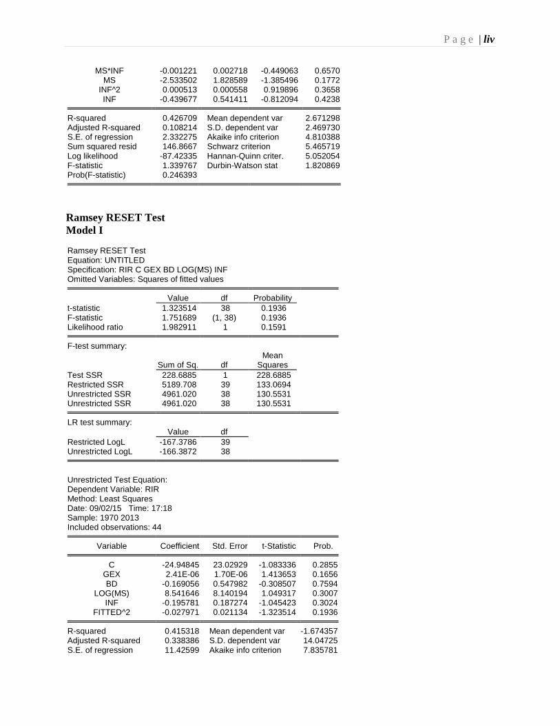
P a g e | liv

MS*INF -0.001221 0.002718 -0.449063 0.6570 MS -2.533502 1.828589 -1.385496 0.1772

INF^2 0.000513 0.000558 0.919896 0.3658 INF -0.439677 0.541411 -0.812094 0.4238



Ramsey RESET Test Model I Ramsey RESET Test Equation: UNTITLED Specification: RIR C GEX BD LOG(MS) INF Omitted Variables: Squares of fitted values

Value df Probability

t-statistic 1.323514 38 0.1936 F-statistic 1.751689 (1, 38) 0.1936 Likelihood ratio 1.982911 1 0.1591

F-test summary:

Sum of Sq. df Mean

Squares Test SSR 228.6885 1 228.6885 Restricted SSR 5189.708 39 133.0694 Unrestricted SSR 4961.020 38 130.5531 Unrestricted SSR 4961.020 38 130.5531

LR test summary: Value df

Restricted LogL -167.3786 39 Unrestricted LogL -166.3872 38

Unrestricted Test Equation: Dependent Variable: RIR Method: Least Squares Date: 09/02/15 Time: 17:18 Sample: 1970 2013 Included observations: 44


GEX 2.41E-06 1.70E-06 1.413653 0.1656 BD -0.169056 0.547982 -0.308507 0.7594

LOG(MS) 8.541646 8.140194 1.049317 0.3007 INF -0.195781 0.187274 -1.045423 0.3024

FITTED^2 -0.027971 0.021134 -1.323514 0.1936 R-squared 0.415318 Mean dependent var -1.674357

Adjusted R-squared 0.338386 S.D. dependent var 14.04725 S.E. of regression 11.42599 Akaike info criterion 7.835781

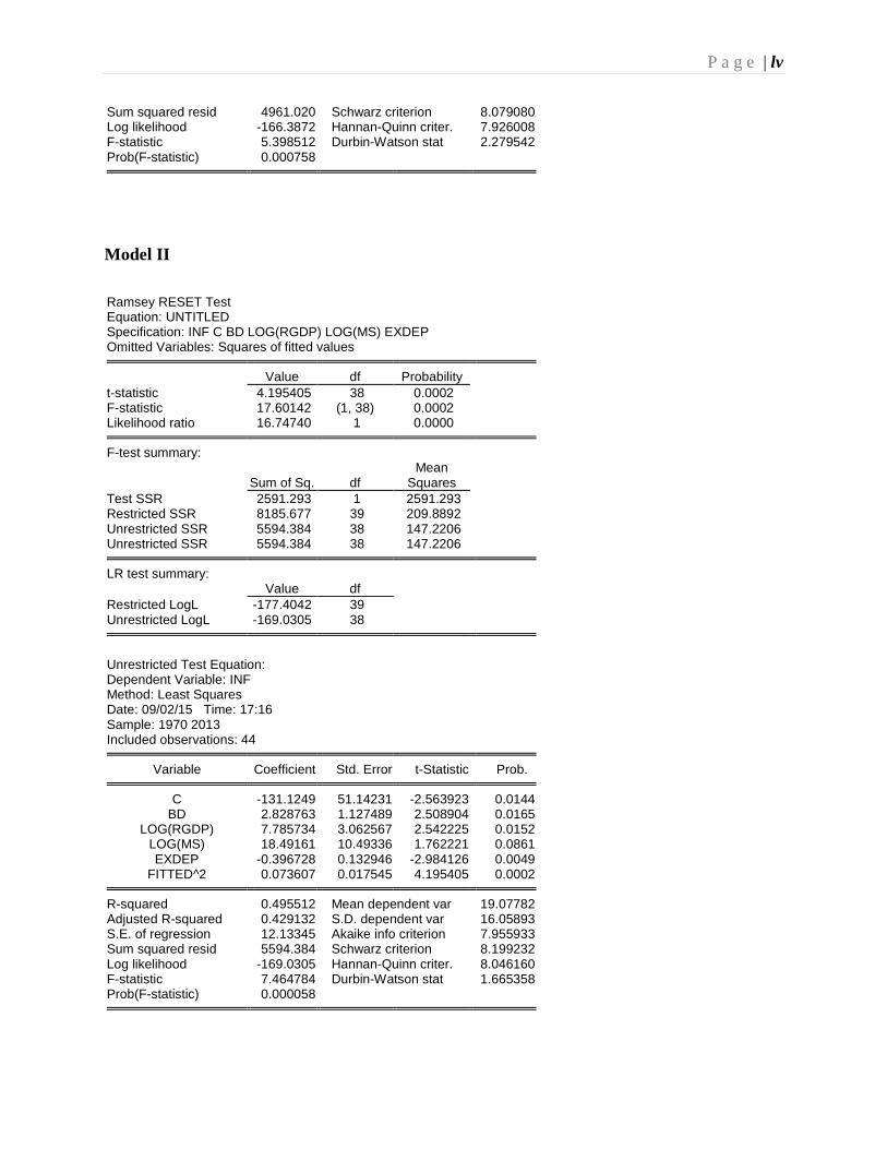
P a g e | lv

Sum squared resid 4961.020 Schwarz criterion 8.079080 Log likelihood -166.3872 Hannan-Quinn criter. 7.926008 F-statistic 5.398512 Durbin-Watson stat 2.279542 Prob(F-statistic) 0.000758

Model II Ramsey RESET Test Equation: UNTITLED Specification: INF C BD LOG(RGDP) LOG(MS) EXDEP Omitted Variables: Squares of fitted values



F-test summary:

Sum of Sq. df Mean




Unrestricted Test Equation: Dependent Variable: INF Method: Least Squares Date: 09/02/15 Time: 17:16 Sample: 1970 2013 Included observations: 44


BD 2.828763 1.127489 2.508904 0.0165 LOG(RGDP) 7.785734 3.062567 2.542225 0.0152

LOG(MS) 18.49161 10.49336 1.762221 0.0861 EXDEP -0.396728 0.132946 -2.984126 0.0049

FITTED^2 0.073607 0.017545 4.195405 0.0002 R-squared 0.495512 Mean dependent var 19.07782


P a g e | lvi

Model III Ramsey RESET Test Equation: UNTITLED Specification: LOG(RGDP) C INF LOG(SAV) RIR BD Omitted Variables: Squares of fitted values



F-test summary:

Sum of Sq. df Mean




Unrestricted Test Equation: Dependent Variable: LOG(RGDP) Method: Least Squares Date: 09/02/15 Time: 17:14 Sample: 1970 2013 Included observations: 44

Variable Coefficient Std. Error t-Statistic Prob. C 21.86404 16.52884 1.322781 0.1938

INF 0.180836 0.188766 0.957990 0.3441 LOG(SAV) 9.133090 9.522567 0.959100 0.3436

RIR 0.236568 0.246135 0.961131 0.3426 BD 0.022446 0.060217 0.372760 0.7114

FITTED^2 -0.240853 0.293425 -0.820831 0.4169 R-squared 0.273250 Mean dependent var 11.97732


P a g e | lvii

Documents

The Effects of Budget Deficits on Selected Macroeconomic