The effect of subgrid-scale models on the entrainment of a

Journal of Turbulence, 2015Vol. 16, No. 4, 342–366, http://dx.doi.org/10.1080/14685248.2014.986329

The effect of subgrid-scale models on the entrainment of a passivescalar in a turbulent planar jet

Carlos B. da Silvaa∗, Diogo C. Lopesa and Venkat Ramanb

aLAETA, IDMEC, Instituto Superior Tecnico, Universidade de Lisboa, Av. Rovisco Pais, 1049-001Lisboa, Portugal; bDepartment of Aerospace Engineering and Engineering Mechanics, The

University of Texas at Austin, Austin, Texas 78712, USA

(Received 14 July 2014; accepted 5 November 2014)

Classical large-eddy simulation (LES) modelling assumes that the passive subgrid-scale (SGS) models do not influence large-scale quantities, even though there is nowample evidence of this in many flows. In this work, direct numerical simulation (DNS)and large-eddy simulations of turbulent planar jets at Reynolds number ReH = 6000including a passive scalar with Schmidt number Sc = 0.7 are used to study the effect ofseveral SGS models on the flow integral quantities e.g. velocity and scalar jet spreadingrates. The models analysed are theSmagorinsky, dynamic Smagorinsky, shear-improvedSmagorinsky and the Vreman. Detailed analysis of the thin layer bounding the turbulentand non-turbulent regions – the so-called turbulent/non-turbulent interface (TNTI) –shows that this region raises new challenges for classical SGS models. The small scalesare far from equilibrium and contain a high fraction of the total kinetic energy and scalarvariance, but the situation is worse for the scalar than for the velocity field. Both a-prioriand a-posteriori (LES) tests show that the dynamic Smagorinsky and shear-improvedmodels give the best results because they are able to accurately capture the correctstatistics of the velocity and passive scalar fluctuations near the TNTI. The results alsosuggest the existence of a critical resolution !x, of the order of the Taylor scale λ, whichis needed for the scalar field. Coarser passive scalar LES i.e. !x ≥ λ results in dramaticchanges in the integral quantities. This fact is explained by the dynamics of the smallscales near the jet interface.

Keywords: turbulent entrainment; large-eddy simulation (LES); jet; turbulent/non-turbulent interface (TNTI); passive scalar

1. Introduction

One of the most distinctive features observed in turbulent free shear flows, such as jets,wakes and mixing layers, is their tendency to slowly spread in the normal direction ofthe flow. The observed spreading can be explained both as a consequence of the turbulententrainment mechanism, whereby irrotational fluid outside the core turbulent region isdrawn into it, or as resulting from the existence of an unbounded region of turbulent flowwith weak kinetic energy dissipation.

The spreading is manifested by the lateral growth of the turbulent/non-turbulent in-terface (TNTI), which is the very sharp region, continually deformed by a wide range ofscales, that marks the transition between the irrotational and turbulent flow regions. Theimportance of the flow dynamics near this interface and of the flow mechanisms associated

∗Corresponding author. Email: [email protected]

C⃝ 2015 Taylor & Francis

Dow

nloa

ded

by [b

-on:

Bib

liote

ca d

o co

nhec

imen

to o

nlin

e U

TL] a

t 09:

06 2

6 Ja

nuar

y 20

15

http://dx.doi.org/10.1080/14685248.2014.986329

mailto:[email protected]

Journal of Turbulence 343

with the entrainment cannot be overemphasised since they determine many of the criticalflow features. The spreading rate of wakes, the exchanges of mass across mixing layers,and the mixing and reaction rates in jets are largely determined by the flow dynamics in thevicinity of the TNTI. Turbulent entrainment is, therefore, of central importance to manynatural and engineering flows.

Past studies described turbulent entrainment as being caused by large-scale eddy mo-tions occurring from time to time at particular locations along the TNTI [5] (engulfment),but recent works suggest instead that the entrainment results mainly from small-scale eddymotions (nibbling) acting along the entire TNTI (Mathew and Basu,[6] Hunt et al. [7]), asoriginally described by Corrsin and Kistler.[8] More recently, the study of the Lagrangiantrajectories of fluid particles near the TNTI [9] and the analysis of the irrotational bubblesexisting inside jets [10] have shown that, at least for jets at the self-similar far-field region,engulfment is virtually inexistent. Reference [11] reviews the recent progress obtained inanalysing the characteristics and flow dynamics near the TNTI.

Since at least for some flows, the turbulent entrainment is caused by the action of thesmallest scales of motion, new questions arise in the context of large-eddy simulations(LES). In LES, the large scales of motion are explicitly computed while the effect of thesmall unresolved scales is modelled by a subgrid-scale (SGS) model.[12] Specifically, itis well known that mixing rates at the edges of jets and mixing layers are governed bythe nearby velocity fluctuations. Arguably, a deficient or inaccurate modelling of thesefluctuations near the TNTI can potentially lead to a deficient prediction of the scalar mixingnear the TNTI and to inaccurate reaction rates in jets.[13]

Some authors argue that even though the entrainment is caused by the action of thesmallest scales of motion, the entrainment rate is imposed by the large-scale eddies, andtherefore no major role should be caused by possible inaccuracies of the SGS models, atleast in the large-scale features of the flows such as their spreading rates, because theseeddies are fully resolved in LES.

There are however situations in which the details of the small-scale nibbling motionsmay be important. The mixing of scalars near the edge of a jet may be such a case because,as is well known, passive scalar mixing always involves two stages: stirring and (small scale)mixing [14] the latter being largely determined by the small scales of the velocity field.Recall that important velocity fluctuations exist in the irrotational flow region adjacent tothe TNTI and that these generate important Reynolds stresses near the jet edge [15–17] andit is these stresses that should ultimately determine the spreading rate of the scalar fields.Moreover, accurate LES near these interfaces may require a minimum local resolution tocapture the correct mixing characteristics.

Da Silva [18] has analysed the SGS dynamics near the TNTI in temporal turbulent jets. Itwas shown that the SGSs of motions (for the velocity field) near the TNTI are far from equi-librium and that they contain an important fraction of the total kinetic energy. Both observa-tions are in strong contrast with the classical assumptions used in LES. Moreover, a-prioritests suggested that the Smagorinsky constant CS needs to be corrected near the jet edge andthe method used to obtain the dynamic Smagorinsky constant CD is not able to cope with theintermittent nature of this region. However, the momentum spreading rate and the centrelinevelocity decay from several LES did not show to be significantly different to the valuesobserved in direct numerical simulation (DNS) of the same flow, at least for small times.Thus, regarding the influence of the SGS models in the global, large-scale flow featuresthese results were inconclusive due to the temporal simulation approach used in that study.

However, recently Gampert et al. [19] have shown that LES do not necessarily capture thecorrect spreading rates in spatially evolving circular jets. Specifically, they have showed that

Dow

nloa

ded

by [b

-on:

Bib

liote

ca d

o co

nhec

imen

to o

nlin

e U

TL] a

t 09:

06 2

6 Ja

nuar

y 20

15

344 C.B. da Silva et al.

coarse grid resolutions tend to underestimate the centreline velocity and passive scalar decayrates, and tend to diffuse the TNTI location, as compared to values observed in experimentalmeasurements. These results clearly show, as suggested before in Ref. [18], that LES doesaffect the TNTI dynamics and the determination of some of the global flow features suchas the jet spreading rate. Furthermore, it also confirmed that the passive scalar field is moreaffected than the velocity field by the limitations of the SGS models near the TNTI.

However, not much information is available concerning the effect of the SGS mod-els and the resolution requirements for an accurate LES of the passive scalar mixingat the edges of jets. Moreover, several SGS models exist and almost no information existson the accuracy and performance of the several existing models for accurate simulation ofthe scalar mixing near the TNTI, which is critical to determine the reaction rates in reactiveflows. The dynamics of the passive scalar near TNTIs itself is poorly understood. Some ofthe few exceptions are presented in the works of Westerweel et al. [20] and in the works ofPeters and co-authors [19,21–24] and of Attili et al. [25]. Westerweel et al. [20] analysedthe conditional profiles (in relation to the TNTI location) of the passive scalar field in ex-perimental round jets. The profiles exhibit much steeper gradients than the ones observedin the velocity field, but the experiments were carried out with a very high Schmidt number.They also provide models for the passive scalar statistics near the TNTI. Gampert et al. [21]established the scaling of the TNTI layer for the scalar field using experimental data froma round jet and concluded that the thickness of this layer is of the order of the Taylor scale,while Gampert et al. [22] analysed the statistics of the scalar dissipation near the TNTI inthe same jet.

The goal of this work is to assess the SGS dynamics and the performance of severalSGS models in handling the particular LES challenges arising when simulating the flownear TNTI interfaces. For this purpose direct numerical and large-eddy simulations ofspatially evolving turbulent plane jets were used. The models analysed in this study are theSmagorinsky, dynamic Smagorinsky,[2] shear-improved Smagorinsky,[3] and the Vreman[4] models. The turbulent plane jet was chosen for this study because it is a canonical flowdisplaying many features that are also common to other free shear layers such as circularjets, wakes and mixing layers.

This paper is organised as follows. The next section (Section 2) describes the fourSGS models assessed in this study. Section 3 describes the direct numerical and large-eddysimulations carried out in this work. The study is based on a new reference DNS whereextensive validation tests were undertaken. Section 4 analyses the SGS dynamics for thevelocity and passive scalar fields near the TNTI, and presents several a-priori tests for thevelocity and scalar fields using the four SGS models. Section 5 discusses the key globalflow quantities obtained from several LES. The paper ends in Section 6 with an overviewof the main results and conclusions.

2. Subgrid-scale models

Several LES were carried out using four different SGS models. The residual or SGS stressestensor arising from spatially filtering the Navier–Stokes equations is τR

ij = uiuj − ui uj ,where the overbar represents a spatial filtering operation. All the SGS models used hererely on the eddy viscosity concept; therefore, only the anisotropic part of the residualstresses defined as τ r

ij = τRij − 1

3τRkkδij requires modelling. The residual SGS stresses are

therefore given by τ rij = −2νT Sij , where νT (x, t) is the turbulent viscosity and Sij =(

∂ui/∂xj + ∂uj∂xi

)is the filtered rate-of-strain tensor.

Dow

nloa

ded

by [b

-on:

Bib

liote

ca d

o co

nhec

imen

to o

nlin

e U

TL] a

t 09:

06 2

6 Ja

nuar

y 20

15


The usual way to construct a model for the passive scalar field φ consists in defining aSGS Schmidt number ScT whereby a scalar diffusivity γT (x, t) is locally defined through

γT (x, t) = νT (x, t)/ScT , (1)

and usually one uses a constant ScT = 1.0 for all the simulation domain. With this approx-imation, the unknown SGS scalar fluxes qj = φuj − φuj , which need to be modelled inLES with passive scalars, can be simply computed through

qj = −γT Gj = −νT /ScT Gj , (2)

where Gj = ∂φ/∂xj is the resolved scalar gradient.

2.1. Smagorinsky model

The Smagorinsky model [1] is used here as a reference SGS model. This model is basedon the assumption of local grid/SGS equilibrium. The eddy viscosity is computed usingνT (x, t) = (CSmag

S !)2|S|, where |S| = (2SijSij )1/2, and ! = (!x!y!z)1/3. The model con-stant C

SmagS is flow dependent but assuming local isotropic turbulence it can be expressed as

CSmagS ≈ 1

π

( 23CK

)3/4, where CK is the Kolmogorov constant. In this work, we use the refer-

ence value of CSmagS = 0.16. The limitations of this model have been repeatedly discussed

i.e. it is a purely dissipative model and is too dissipative.[26]

2.2. Dynamic Smagorinsky model

In the dynamic Smagorinsky model, [2] the model constant CD(x, t) = (CSmagS )2 is com-

puted in space and time using the Germano identity resulting in [26] CD(x, y, t) =⟨MijLij⟩/⟨MijMij⟩, where Lij = ui uj − ui uj is the Leonard stresses tensor defined with

a spatial ‘test’ filter with size 2!, and Mij = −(k!)2 |S|Sij + !2 |S|Sij . The constant khas an optimum value of k =

√5 for a test filter size of 2! as detailed in [27]. The angle

brackets indicate space averaging along the homogenous directions of the flow, which inthe case of a planar jet, is the spanwise (z) direction only. In the present simulations, it wasobserved that CD(x, y, t) computed as described above seldom results in negative values.Nevertheless clipping to zero was applied to CD(x, y, t) whenever CD(x, y, t) ≤ 0.

2.3. Shear-improved Smagorinsky model

One of the drawbacks of the Smagorinsky model is that the turbulent viscosity is largein flow regions where the mean flow gradient is large, even if the local level of velocityfluctuations is not strong. In the shear-improved Smagorinsky model introduced by Levequeet al., [3] the Smagorinsky model is modified by removing the mean strain rate from the(total) strain rate magnitude used in the definition of the turbulent viscosity. The turbulentviscosity is computed as νT (x, t) = (CS!)2(|S| − |⟨S⟩|), where the brackets indicate aspace average along the spanwise direction.

Dow

nloa

ded

by [b

-on:

Bib

liote

ca d

o co

nhec

imen

to o

nlin

e U

TL] a

t 09:

06 2

6 Ja

nuar

y 20

15


2.4. Vreman model

The Vreman model [4] is also designed to eliminate excessive dissipation of the Smagorin-sky model in regions where the flow is laminar or transitional but where the mean strainrate is large. The model does not require the existence of homogenous directions to performaverages, or the application of clipping procedures to prevent negative values of turbulentviscosity and is therefore well suited for engineering applications. The turbulent viscosity isgiven by νT (x, t) = 2.5C2

S

√Bβ/(αijαij ), where αij = ∂uj/∂xi , and βij = !2

mαmiαmj , withBβ = β11β22 − β2

12 + β11β33 − β213 + β22β33 − β2

23. The tensor β ij is positive semidefinite,and therefore Bβ ≥ 0. If αijαij is equal to zero, the turbulent viscosity is consistently definedas zero.

3. Direct and large-eddy simulations of turbulent planar jets

This section describes the direct and large-eddy simulations carried out in this work. Thesimulations were performed with an upgraded version of the same solver used in da Silvaand Metais. [28] The new solver uses massive use of message passing interface (MPI)libraries for parallel domain decomposition, written in Fortran 95, and uses the fast Fouriertransform in the West (FFTW) library for Fast-Fourier Transform algorithm. Full detailsare given in Reis.[29] Moreover, the transport of a passive scalar filed was added to thenumerical algorithm.

3.1. Numerical methods

The computational domain consists in a box with sizes Lx, Ly and Lz along the streamwise(x), normal (y) and spanwise (z) directions, respectively. The simulations were carriedout with an incompressible Navier–Stokes solver using mixed pseudo-spectral/‘Compact’finite-differences for spatial discretisation: a sixth-order Compact scheme (Lele [30]) isused to compute the derivatives in the streamwise (x) direction, while a pseudo-spectralscheme (Canuto et al. [31]) is used for derivatives in the normal (y) and spanwise (z)directions. For temporal advancement, the algorithm uses an explicit three-step third-order low-storage Runge–Kutta time-stepping scheme (Williamson [32]). Pressure velocitycoupling is achieved with a fractional step method (Kim and Moin [33]; Le and Moin [34])ensuring mass conservation at each sub-step of the Runge–Kutta time-advancing scheme.In addition to the Navier–Stokes equations, the evolution of a passive scalar field is addedto the simulations. The passive scalar is numerically simulated by solving a convection-diffusion equation employing the same numerical schemes used for the computation ofthe velocity field, except for the convective terms which are discretised using a QUICKscheme.[35]

For boundary conditions, the code uses a non-reflective (Orlansky [36]) outflow condi-tion in the streamwise direction (x), while the spanwise (z) direction is treated as periodic.The boundaries in the normal (y) direction were also treated as periodic. Such boundaryconditions, which permit the use of very accurate pseudo-spectral schemes, do not allowentrainment from the flow situated outside the computational domain. However, as wasshown in e.g. Stanley et al.[37] and da Silva and Metais [28], the imposition of a smallco-flow allows us to obtain a very good statistical concordance with experimental measure-ments as long as the lateral boundary conditions of the jet are placed sufficiently far fromthe turbulent region.

The algorithm is parallelised with MPI as illustrated in Figure 1. Since Compact dif-ferentiation (d/dx) at a point requires a complete line of data along the streamwise (x)

Dow

nloa

ded

by [b

-on:

Bib

liote

ca d

o co

nhec

imen

to o

nlin

e U

TL] a

t 09:

06 2

6 Ja

nuar

y 20

15


(a) (b)

Figure 1. Data distribution among processors (P0, P1, . . . , PN). The conversion between slicesand slabs uses MPI_AlltoAll.(a) Configuration 1: data organised in slices. (b) Configuration 2: dataorganised in slabs.

direction, whereas pseudo-spectral differentiation (d/dy and d/dz) requires complete linesof data along the y and z directions, respectively, for each time step the data fields existin one of two different configurations, depending on which operation is being done. Inconfiguration 1, the data are organised into slices, while in configuration 2 the data areorganised into slabs (see Figure 1). Therefore, once the data are in either configuration,differentiation can be carried out without any further message passing between processors.More details are described in Reis [29].

For inflow conditions, the streamwise velocity (u) and a passive scalar (φ) instantaneousfields are prescribed at the inlet for each time step (the mean normal and spanwise velocitiesare set to zero at the inlet). The mean inlet velocity and passive scalar are based in ahyperbolic tangent profile (Stanley et al.,[37] da Silva and Metais [28]),

U (x = 0, y, z) = U1 + U2

2+ U1 − U2

2tanh

[H

4θ

(1 − 2|y|

H

)], (3)

-(x = 0, y, z) = -1 + -2

2+ -1 − -2

2tanh

[H

4θ

(1 − 2|y|

H

)], (4)

where U1 and -1 are the jet centreline velocity and passive scalar and U2 and -2 is a smallco-flow (of velocity and scalar), respectively. θ is the momentum thickness of the initialshear layer, H is the inlet slot width of the jet and y is the distance from the centre of theshear layer. Notice that (3) and (4) have to be mirrored about the plane (x, z) in order toobtain the desired jet top-hat profile.

A three-component (u, v and w) fluctuating velocity fields were superimposed to themean velocity profile. Each velocity component of the noise is prescribed in such a waythat its energy spectrum was chosen to give an energy input dominant at small scales.The numerical noise was only imposed within the shear-layer region of the mean (stream-wise velocity) profile through a proper convolution function. More details are given inReis [29].

3.2. Physical and computational parameters

A reference DNS of a planar turbulent jet was carried out in a domain with (Lx, Ly, Lz) =(24H, 24H, 4H), where Lx, Ly, and Lz are the spatial extents of the computational domain

Dow

nloa

ded

by [b

-on:

Bib

liote

ca d

o co

nhec

imen

to o

nlin

e U

TL] a

t 09:

06 2

6 Ja

nuar

y 20

15


Table 1. Summary of grids used in the LES. For each grid fourLES were carried out with four different SGS models: Smagorinsky(SMG), dynamic Smagorinsky (DSM), shear-improved (SIM) andVreman (VRM) models.

LES grid Resolution Implicit filter sizeN1 × N2 × N3 (!x/H) (!/λ)

192 × 192 × 32 0.125 0.896 × 96 × 16 0.250 1.648 × 48 × 8 0.500 3.2

along the streamwise (x), normal (y) and spanwise (z) directions, respectively. The grid isuniform in the three spatial directions with !x = !y = !z = 0.016H and the total numberof grid points along these directions is N1 = 1536, N2 = 1536 and N3 = 256, respectively.The Reynolds number is ReH = !UH/ν = 6000, where ν is the kinematic viscosity, and!U = U1 − U2 are the maximum and minimum (co-flow) jet velocities which were set toU1 = 1.182 and U2 = 0.182, respectively.

In the present DNS, the co-flow level is r = U2/U1 ≈ 0.153, which is comparable tothe same ratio used by Le Ribault et al.,[38] Stanley et al.,[37] da Silva and Metais.[28]The slightly higher co-flow level used here is justified by the much bigger extent of thespatial domain used in this work. These studies have demonstrated that such a small co-flowhas only a minor influence on the jet dynamics. As in Stanley et al.,[37] and da Silva andMetais [28] the ratio between the inlet momentum thickness and the inlet slot-width of thejet is H/θ = 30. For the passive scalar field, the maximum and minimum inlet mean scalarwere set to -1 = 1.0 and -2 = 0.0, respectively, and the Schmidt number is SC = 0.7. Themaximum intensity of the inlet velocity fluctuations is 3% of the maximum inlet velocity,U1 and no ‘noise’ was prescribed at the inlet for the passive scalar field.

A set of LES were carried out using the same physical parameters of the reference DNSbut using coarser meshes. Table 1 lists the turbulent planar jet simulations carried out inthis work. The simulations were carried out on 192 processors.

3.3. Assessment of the reference DNS

Figures 2 and 3 show contours of vorticity magnitude and passive scalar, respectively, ina (x, y) plane of the turbulent plane jet DNS. The jet undergoes a classical transition toturbulence prompted by the emergence of the primary instabilities in the form of Kelvin–Helmholtz vortices discernible at x/H ≈ 3 which are initially symmetric (in relation to thejet centreline plane) as predicted by the linear stability theory for this case since H/θ =30. Further downstream e.g. at x/H ≈ 5, the Kelvin–Helmholtz rollers show small-scaleeddies in their interior and streamwise eddies start forming. These secondary structuresquickly become fragmented and by x/H ≈ 9 both the vorticity and passive scalar structuresexhibit a large range of scales and do not show the existence of any preferential direction,sign of a fully developed turbulent state. The passive scalar tends to wrap around the flowvortices and far downstream shows that regions of low scalar concentration exist very closeto the regions of high scalar concentration, with excursions of irrotational (no scalar) flowreaching almost the centreline of the jet in some places.

The present DNS is compared with the experimental data from Browne et al.,[39]Thomas and Chu,[40] Deo et al.,[41,42] Davies et al.,[43] and the DNS of Stanley and

Dow

nloa

ded

by [b

-on:

Bib

liote

ca d

o co

nhec

imen

to o

nlin

e U

TL] a

t 09:

06 2

6 Ja

nuar

y 20

15


Figure 2. Contours of vorticity magnitude (normalised by U1/H) in a (x, y) plane extending from0 < x/H < 24 and −5 < y/H < + 5 for the DNS of the turbulent planar jet. Notice that the figuredoes not show the total extent of the computational domain in the lateral (y) dimension.

Sarkar[44] and da Silva and Metais.[28] Figure 4(a) and 4(b) show the streamwise evolutionof the jet half-width δu(x) defined as ⟨u(y = δu)⟩ = ⟨u(y = 0)⟩/2, and the centreline velocitydecay ⟨uc(x)⟩ = ⟨u(y = 0)⟩, respectively. The brackets represent temporal and spanwiseaverages, followed by ‘folding’ of the mean profiles due to symmetry.

The details of the transition (0 < x/H < 5) differ quite appreciably in all the cases.Specifically, the transition to turbulence in the DNSs takes place later than in the experi-ments. This is caused in part by the Reynolds number in the DNSs being smaller than in theexperiments, and by having a smaller ratio of H/θ as discussed in references.[28,44] In anycase, only the slopes of the curves should be compared since they describe the turbulentflow at the far field, and are independent of the extremely sensitivity of the jet to the inletconditions.

Figure 3. Contours of passive scalar in a (x, y) plane extending from 0 < x/H < 24 and −5 < y/H <+ 5 for the DNS of the turbulent planar jet. Notice that the figure does not show the total extent ofthe computational domain in the lateral (y) dimension.

Dow

nloa

ded

by [b

-on:

Bib

liote

ca d

o co

nhec

imen

to o

nlin

e U

TL] a

t 09:

06 2

6 Ja

nuar

y 20

15


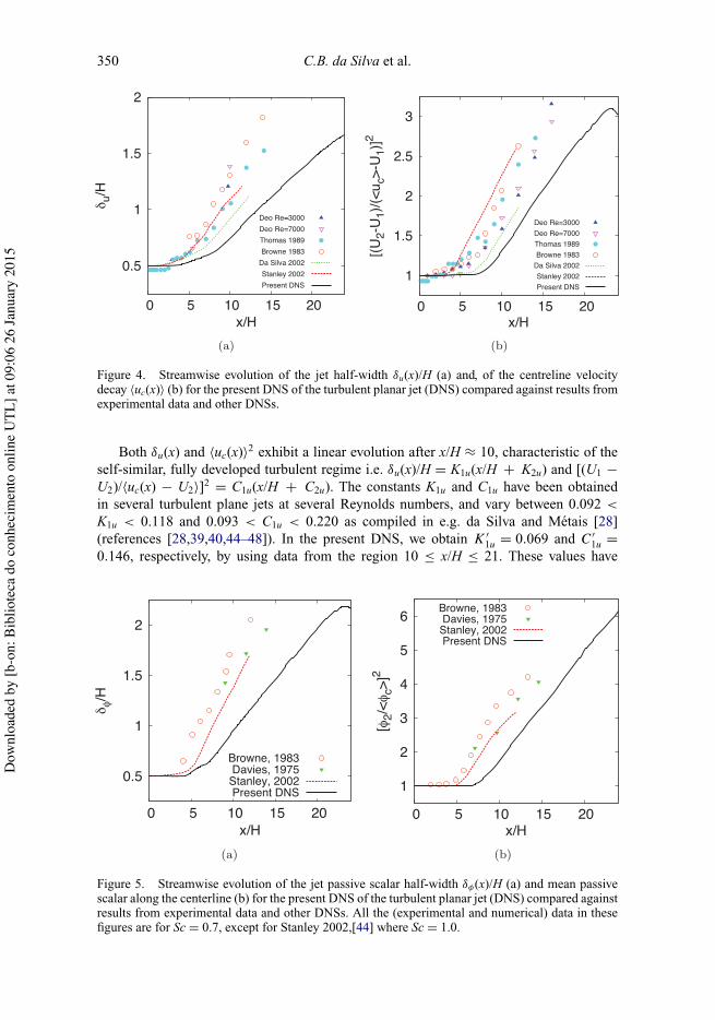
Figure 4. Streamwise evolution of the jet half-width δu(x)/H (a) and, of the centreline velocitydecay ⟨uc(x)⟩ (b) for the present DNS of the turbulent planar jet (DNS) compared against results fromexperimental data and other DNSs.

Both δu(x) and ⟨uc(x)⟩2 exhibit a linear evolution after x/H ≈ 10, characteristic of theself-similar, fully developed turbulent regime i.e. δu(x)/H = K1u(x/H + K2u) and [(U1 −U2)/⟨uc(x) − U2⟩]2 = C1u(x/H + C2u). The constants K1u and C1u have been obtainedin several turbulent plane jets at several Reynolds numbers, and vary between 0.092 <

K1u < 0.118 and 0.093 < C1u < 0.220 as compiled in e.g. da Silva and Metais [28](references [28,39,40,44–48]). In the present DNS, we obtain K ′

1u = 0.069 and C ′1u =

0.146, respectively, by using data from the region 10 ≤ x/H ≤ 21. These values have

Figure 5. Streamwise evolution of the jet passive scalar half-width δφ(x)/H (a) and mean passivescalar along the centerline (b) for the present DNS of the turbulent planar jet (DNS) compared againstresults from experimental data and other DNSs. All the (experimental and numerical) data in thesefigures are for Sc = 0.7, except for Stanley 2002,[44] where Sc = 1.0.

Dow

nloa

ded

by [b

-on:

Bib

liote

ca d

o co

nhec

imen

to o

nlin

e U

TL] a

t 09:

06 2

6 Ja

nuar

y 20

15


Figure 6. Mean streamwise velocity ⟨u(y)⟩ (a), and mean passive scalar concentration ⟨φ(y)⟩ (b)for the DNS of the turbulent plane jet (at x/H = 12, 15, 18 and 21) compared against results fromexperimental data and other DNS.

to be corrected with the co-flow used in order to be compared with the other DNS andexperimental data. Indeed it has been shown by Youssef et al. [49] that above a certainthreshold value of r the co-flow slightly affects the constants K1u and C1u. Correcting thepresent results using the experimental data from Youssef et al., [49] we get K1u = 0.102and C1u = 0.180, respectively, which compares well with the experimental and numericaldata in existence for planar jets.

Similarly to the velocity field, a linear behaviour is expected for the half-width of thepassive scalar field δφ(x), defined as ⟨φ(y = δφ)⟩ = ⟨φ(y = 0)⟩/2, and for the centrelineevolution of the mean passive scalar concentration ⟨φc(x)⟩ defined as ⟨φc(x)⟩ = ⟨φ(y =0)⟩. Specifically, these quantities have been seen to evolve as δφ(x)/H = K1φ[x/H + K2φ],and [(-1 − -2)/(φc − -2)]2 = C1φ[x/H + C2φ], respectively. The constants K1φ and C1φ

from several experimental and numerical works range between 0.115 ≤ K1φ ≤ 0.167 and0.194 ≤ C1φ ≤ 0.308 (see references [39,43,44,47,50]). The present DNS gives K1φ =0.102 and C1φ = 0.317, in reasonable agreement with the available data, considering thelevel of co-flow used.

It is noteworthy that the streamwise evolution of the Reynolds number based onthe Taylor micro-scale Reλ(x) = ⟨u′(x)⟩ ⟨λx(x)⟩/ν, where ⟨λx⟩ 2 = ⟨u′2⟩/⟨(∂u′/∂x)2⟩ and⟨u′(x)⟩ =(⟨u2(x, y = 0)⟩ − ⟨u(x, y = 0)⟩2)1/2, along the centreline of the jet has a constantvalue of Reλ(x) ≈ 110 from x/H ≥ 9 onwards, (not shown) in agreement with the theoreticalresults for the planar turbulent jet, further stressing that the self-similar, fully developedregime has been attained.

Figure 6(a) and 6(b) show the mean streamwise velocity ⟨u(y)⟩ and mean passive scalar⟨φ(y)⟩ profiles for several stations of the planar turbulent jet compared against severalnumerical and experimental data. As can be seen the mean profiles exhibit self-similarityfrom x/H ≥ 9 and agree well with the data available. The streamwise evolution of thenormal Reynolds stresses and passive scalar variance is shown in Figure 7(a) and 7(b),respectively. The normal stresses agree well with the available numerical and experimentaldata (Figure 7(a)), while the scalar variance displays a higher maximum than in the referencedata (Figure 7(b)) which is explained by the later transition observed for the scalar, as

Dow

nloa

ded

by [b

-on:

Bib

liote

ca d

o co

nhec

imen

to o

nlin

e U

TL] a

t 09:

06 2

6 Ja

nuar

y 20

15


Figure 7. Streamwise evolution of the streamwise normal Reynolds stresses ⟨u′2⟩ (a), and passivescalar variance ⟨φ′2⟩ (b) for the DNS of the turbulent plane jet (present DNS)compared against resultsfrom experimental data and other DNS.

discussed in detail in reference [51]. Moreover Figure 8(a) and 8(b) show the profiles of thestreamwise Reynolds stresses ⟨u′2⟩ and passive scalar variance ⟨φ′2⟩ at several streamwiselocations for the present DNS. As can be seen both ⟨u′2⟩ and ⟨φ′2⟩ display a self-similarbehaviour for x/H ≥ 12 for the velocity, and for x/H ≥ 15 for the scalar, respectively.

Figure 9(a) and 9(b) show the probability density functions (pdfs) across the jet i.e.for several distances from the jet centreline (0 ≤ y/δφ ≤ 5) at two stations x/H = 8 andx/H = 20, respectively. The first figure shows that the pdfs exhibit a peak at φ = 0.5for two distances from the centreline (y/δφ = 0 and y/δφ = 1.38). The pdfs thus exhibit

Figure 8. Profiles of the streamwise normal Reynolds stresses ⟨u′2⟩ (a), and passive scalar variance⟨φ′2⟩ (b) at several downstream locations for the DNS of the turbulent plane jet (at x/H = 12, 15, 18and 21) compared against results from experimental data and other DNS.

Dow

nloa

ded

by [b

-on:

Bib

liote

ca d

o co

nhec

imen

to o

nlin

e U

TL] a

t 09:

06 2

6 Ja

nuar

y 20

15


Figure 9. Probability density functions of passive scalar across the jet at (a) x/H = 8, and at x/H =20 (b).

a non-marching behaviour which is typical of the transition region in the jet, where at agiven position and for a given time we find either maximum scalar concentration φ = 1 orno scalar concentration at all φ = 0. In contrast at x/H = 20 the pdfs exhibit a marchingbehaviour where the location of the maximum of the pdfs changes across the jet i.e. themaximum of the pdfs decreases from φ = 0.5 to φ = 0.25 as we move from y/δφ = 0 toy/δφ = 1.46. It is well known [52] that this behaviour is the imprint of a fully developedturbulent state and characteristic of high Reynolds numbers flows. Analysis of the pdfs atseveral stations shows that the switch between non-marching to marching pdfs takes placeapproximately between 9 ≤ x/H ≤ 12. Therefore, the passive scalar field is characteristicof fully developed turbulence from x/H ≥ 12. This is consistent with the visualisations ofpassive scalar shown in Figure 3.

To complete the assessment of the DNS, Figure 10(a) and 10(b) show spectra computedfrom temporal kinetic energy and passive scalar signals taken from the centreline of thejet at x/H = 20. As can be seen both spectra display an inertial range of scales, showinga power-law scaling of −5/3. A very similar spectrum is already present at x/H = 12(not shown). At the highest frequencies, the spectra show a smooth transition to negligiblevalues of energy, consistent with a well-resolved simulation. The resolution was assessedby comparing the grid size with the Kolmogorov micro-scale η = (ν3/ε)1/4, both along thestreamwise direction x as along the normal jet direction y. The figures (not shown) indicatethat the resolution of the present DNS from x/H ≥ 12 is always !x/⟨η(x, y)⟩ ≤ 2.5, thusconfirming that the DNS is indeed well resolved.

4. Characteristics of the TNTI region in a jet and consequences for large-eddysimulations

In this section, we describe the SGS interactions at the jet edge and analyse the SGSdynamics for the velocity and scalar fields, using the reference DNS. This information islater used to assess the effect of several SGS models in the local (near the TNTI) and in theglobal jet characteristics in LES of turbulent jets.

Dow

nloa

ded

by [b

-on:

Bib

liote

ca d

o co

nhec

imen

to o

nlin

e U

TL] a

t 09:

06 2

6 Ja

nuar

y 20

15


Figure 10. (a) Kinetic energy spectrum at the jet centreline at x/H = 20. (b) Passive scalar variancespectrum at the jet centreline at x/H = 20.

4.1. Conditional statistics in relation to the distance from the TNTI location

Conditional statistics in relation to the distance from the TNTI position were computed.Similar statistics have been used in a number of works (Refs [16,20,24,53]) and thereforeonly a short description is given here.

The location of the TNTI is defined by the surface where the vorticity norm ω =(ωiωi)1/2 is equal to a certain threshold ω = ωtr, where the particular value of this thresholdhas been computed as described in Ref. [53]. In short, the volume of the turbulent regionVT depends on the particular value of the vorticity threshold used to defined it ωtr, andwhen plotting this dependency i.e. VT = VT(ωtr), a small plateau is observed where thevolume of the turbulent region changes slowly with the ωtr. In practice, any value of theωtr taken from this plateau allows the sharp TNTI region to be defined. More details can befound in reference [10]. Notice that the particular value of the vorticity magnitude detectionthreshold ωtr, changes with x because as the jet develops, the mean vorticity magnitudeat the jet edge (as inside the turbulent region) decreases making the use of a constant ωtr

unsuited to locate the TNTI for all stations. Therefore, the determination of ωtr was doneinvolving data from slices of size H around each particular station. A local coordinatesystem located at the TNTI is then used to compute statistics as function of the distanceto the TNTI location where a total of 100 instantaneous fields is used to obtain convergedstatistics. In the resulting conditional mean profile, the TNTI is located at yI = 0, whilethe irrotational and turbulent regions are defined by yI < 0 and yI > 0, respectively. Thedistance from the TNTI in the conditional profiles is given both in units of inlet slot-widthH and Taylor micro-scale λ, where the Taylor micro-scale is taken from the jet centrelineand is equal to λ/H ≈ 0.11 for x/H = 15. Figure 11 shows the conditional spanwise vorticitymagnitude |ωz| at 14 < x/H < 15 normalised by the inlet velocity U1 and inlet slot-width ofthe jet H. In agreement with numerous experimental and numerical works (e.g. references[20,24] and [54]) |ωz| exhibits a sharp jump at the TNTI and is roughly constant inside theturbulent region. The thickness of this jump is comparable to the Taylor micro-scale and themagnitude of |ωz| in the turbulent region agrees also with values from previous numericalsimulations of turbulent planar jets.

Dow

nloa

ded

by [b

-on:

Bib

liote

ca d

o co

nhec

imen

to o

nlin

e U

TL] a

t 09:

06 2

6 Ja

nuar

y 20

15


Figure 11. Conditional mean profile (in respect to the TNTI position located at yI = 0) of spanwisevorticity ⟨|ωz|⟩I at station 14 < x/H < 15, in units of H and in units of λ, where λ is taken from insidethe turbulent region, for the reference DNS.

Figure 12. Conditional mean profiles of (a) streamwise velocity ⟨ux⟩I and (b) passive scalar ⟨φ⟩I (inrespect to the TNTI position located at yI = 0) at station 14 < x/H < 15, in units of H and in units ofλ, where λ is taken from inside the turbulent region, for the reference DNS.

It is interesting to compare the conditional mean profiles of some quantities for thevelocity and the passive scalar fields. For this purpose, Figures 12(a), 12(b), 13(a) and13(b) show the mean profiles of streamwise velocity ⟨ux⟩I, passive scalar ⟨φ⟩I, spanwisevorticity magnitude ⟨|ω|⟩I and passive scalar gradient magnitude ⟨(GjGj)1/2⟩I, respectively,for station 14 < x/H < 15. Again all the quantities are normalised by U1 and H.

Dow

nloa

ded

by [b

-on:

Bib

liote

ca d

o co

nhec

imen

to o

nlin

e U

TL] a

t 09:

06 2

6 Ja

nuar

y 20

15


The conditional profiles agree well with previous published data (e.g. Westerweel et al.[20] and Gampert et al. [24]): the velocity exhibits a small jump right at the start of the TNTI(only for the last flow stations in agreement with [55]), and the vorticity jump has a thicknesswhich is δω ∼ λ in agreement with da Silva and Taveira.[54] On the other hand, both thepassive scalar and passive scalar gradients exhibit much sharper gradients (Figures 12(b)and 13(b)) in agreement with Westerweel et al.,[20] Gampert et al. [22,24] and Attili et al.[25]. The strong overshoot of the scalar gradient can be explained by the characteristiccliff-ramp structure of the scalar field, and by these structures being continually ‘defining’the TNTI.[24]

Finally, Figure 14 shows the conditional mean streamwise velocity and passive scalarvariance profiles, ⟨u′2⟩I and ⟨φ′2⟩I at stations 14 < x/H < 15. As can be seen there areimportant velocity fluctuations originated in the irrotational flow region, which is a well-known fact (e.g. Phillips [15]), while this is not the case for the passive scalar. The anisotropyof the large scales of the flow in the turbulent region can be clearly observed by the fact thatboth ⟨u′2⟩I and ⟨φ′2⟩I are not constant inside the turbulent region. Indeed both quantitiesdecay near the jet centreline, displaying maxima near the jet edge. Again the superiorsharpness of the spatial gradients associated with the passive scalar as compared to thevelocity field can be noticed.

4.2. Analysis of the subgrid-scale interactions at the jet edge

The SGS dynamics near the TNTI was analysed for stations 14 < x/H < 15 using conditionalstatistics in relation to the TNTI position as described in the previous section. The separationbetween grid and SGSs is accomplished by using a box filter with three different filter sizes!. In terms of the Taylor scale of the flow (taken from the turbulent region) the three filtersizes have lengths equal to !/λ = 0.8, 1.6 and 3.2, respectively.

Figure 15(a) shows conditional profiles of the ratio between the unresolved and resolvedkinetic energy defined by ⟨τR

ii ⟩I /⟨uiui⟩I , where the ‘bar’ represents the spatial filtering

Figure 13. Conditional mean profiles of (a) vorticity magnitude ⟨ω⟩I and (b) scalar gradient magni-tude ⟨GjGj⟩I (in respect to the TNTI position located at yI = 0) at station 14 < x/H < 15, in units ofH and in units of λ, where λ is taken from inside the turbulent region, for the reference DNS.

Dow

nloa

ded

by [b

-on:

Bib

liote

ca d

o co

nhec

imen

to o

nlin

e U

TL] a

t 09:

06 2

6 Ja

nuar

y 20

15


Figure 14. Conditional mean profile (in respect to the TNTI position located at yI = 0) of streamwisevelocity and passive scalar variance ⟨u′2⟩I and ⟨φ′2⟩I at stations 14 < x/H < 15, in units of H and inunits of λ, where λ is taken from inside the turbulent region, for the reference DNS.

operation and τRij is the SGS stresses tensor. The mean profiles show that the kinetic energy

at the unresolved scales increases as one approaches the TNTI in agreement with reference[18]. For the bigger filter size (!/λ = 3.2), roughly 8%–10% of the energy at the jet centreis in the SGSs, which is representative of a typical good LES, but this fraction rises to≈25% at the jet edges, which is clearly outside the classical assumptions used in LES.

To analyse the SGS interactions near the TNTI, Figure 15(b) plots the kinetic energy SGSproduction 1 = −τR

ij sij , and the passive scalar SGS production 1φ = −qjGj , respectively,where sij and Gj = ∂φ/∂xj are the resolved rate-of-strain and resolved scalar gradient,respectively, and qj = ujφ − ujφ is the SGS scalar flux. Recall that 1 > 0 represents adirect kinetic energy cascade i.e. energy flux from resolved into unresolved scales, while 1

< 0 represents a reversed or inverse energy cascade, from unresolved into resolved scales(same meaning for 1φ > 0 and 1φ < 0 for the passive scalar). As can be seen the meanenergy cascade fluxes represent only direct cascade i.e. ⟨1⟩I > 0 and ⟨1φ⟩I > 0. Howeverthe production of velocity and scalar SGSs is markedly different. For the passive scalar,a distinct maximum mean production occurs near the TNTI, while for the velocity thiscorresponds roughly to the location of the maximum Reynolds stresses (see Figure 14).

Figure 15(c) shows the conditional mean molecular dissipations of kinetic energy ε =2νsijsij and passive scalar variance εφ = γ GjGj, respectively, where one can see that bothquantities are again quite different. Whereas the dissipation of energy increases in theturbulent region, the dissipation of scalar variance quickly rises to a plateau once the TNTIis crossed into the turbulent region.

Figure 15(d) displays the conditional mean profile of the ratio between the energy andscalar variance SGS production (1 and 1φ) and molecular dissipation (ε and εφ), for thekinetic energy and scalar variance, respectively i.e. ⟨1⟩I/⟨ε⟩I and ⟨1φ⟩I/⟨εφ⟩I. In da Silva

Dow

nloa

ded

by [b

-on:

Bib

liote

ca d

o co

nhec

imen

to o

nlin

e U

TL] a

t 09:

06 2

6 Ja

nuar

y 20

15


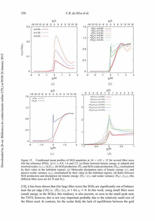
Figure 15. Conditional mean profiles of SGS quantities at 14 < x/H < 15 for several filter sizes(for the reference DNS). !x/λ = 0.8, 1.6 and 3.2: (a) Ratio between kinetic energy at subgrid andresolved scales ⟨τii⟩I /⟨uiui⟩I . (b) SGS production ⟨1⟩I and SGS scalar production ⟨1φ⟩I (normalisedby their value in the turbulent region). (c) Molecular dissipation rates of kinetic energy ⟨ε⟩I andpassive scalar variance ⟨εφ⟩I (normalised by their value in the turbulent region). (d) Ratio betweenSGS production and dissipation for kinetic energy ⟨1⟩I/ ⟨ε⟩I; and scalar variance ⟨1φ⟩ I/⟨εφ⟩I (thedifferent filter sizes are for 1 and 1θ ).

[18], it has been shown that (for large filter sizes) the SGSs are significantly out of balancenear the jet edge [18] i.e. ⟨1⟩I /⟨ε⟩I = 1 for yI ≈ 0. In this work, using small filter sizes(small energy in the SGSs), this tendency is also present, as seen in the small peak nearthe TNTI; however, this is not very important probably due to the relatively small size ofthe filters used. In contrast, for the scalar field, the lack of equilibrium between the grid

Dow

nloa

ded

by [b

-on:

Bib

liote

ca d

o co

nhec

imen

to o

nlin

e U

TL] a

t 09:

06 2

6 Ja

nuar

y 20

15


and SGSs of the scalar is clearly apparent ⟨1φ⟩I /⟨εφ⟩I = 1, which suggests a challengingsituation for SGS modelling of the scalar field.

To summarise, the analysis of the SGS dynamics allows one to conclude already a factthat had been only hinted in da Silva [18]: that SGS modelling is more challenging for thepassive scalar than for the velocity field. Indeed, the gradients of the scalar quantities aremuch stronger than their velocity counterparts and their maxima tend to locate near thejet edge, precisely the region where turbulent mixing is taking place. Moreover the lack ofbalance between production and dissipation of SGS scalar (which is something for whichclassical eddy viscosity SGS models are not designed to deal with) raises challenges forthe SGS modelling of the scalar near the TNTI.

Finally, these results i.e. the significant differences observed in the SGS quantities forthe velocity and scalar fields suggest that the common turbulent diffusivity hypothesis(Equation (1)) is a crude approximation at best. Indeed, as is well known the eddy viscosityapproximation is already a poor local approximation since the correlation between τ ij andsij is roughly 20%, [56] and given the sharp differences between e.g. sij (proportional tothe viscous dissipation ε) and εφ the situation should be even more critical for the scalar.Notice that the present DNS is carried out with the most favourable possible situationin this respect because Sc ≈ 1, should imply a similar ‘sharpness’ between sij and Gj

deep inside the turbulent region. It is expectable that the local gradients of Gj near theTNTI will tend to increase/decrease with the Schmidt number, therefore, suggesting that forSc ≫ 1 or Sc ≪ 1 the turbulent diffusivity approximation will tend to be even more at oddswith the reality.

4.3. A-priori tests at the jet edge

We now turn into classical a-priori tests near the jet edge for the four SGS models describedin Section 2: Smagorinsky (Smag.), dynamic Smagorinsky (DySm.), Vreman (Vrem.) andshear-improved Smagorinsky (SIS).

By equating the real and modelled SGS production ⟨1DNS⟩I = ⟨1Smag.⟩I, one obtainsthe following expression for the Smagorinsky constant CS (see references [12,56,57]),

⟨C2

S

⟩I

=⟨− τR

ij sij

⟩I

⟨2!2|S|smnsmn⟩I. (5)

In isotropic turbulence, by invoking local equilibrium and an inertial range energy spectrum

CS = 1π

(2

3Ck

)= 0.16 is obtained for a Kolmogorov constant equal to Ck = 1.6.

For the dynamic Smagorinsky, the model constant is given by

⟨CD⟩I = ⟨LijMij ⟩I⟨MijMij ⟩I

, (6)

with Lij (Leonard) and Mij tensors defined before. In the shear-improved model, the constantis computed through

⟨C2

S

⟩I

=⟨− τR

ij sij

⟩I

⟨2!2(|S| − |⟨S⟩|)smnsmn⟩I, (7)

Dow

nloa

ded

by [b

-on:

Bib

liote

ca d

o co

nhec

imen

to o

nlin

e U

TL] a

t 09:

06 2

6 Ja

nuar

y 20

15


Figure 16. Conditional mean profiles of models constants in respect to the TNTI at station 14 <x/H < 15, for a filter size of 3.2λ using the reference DNS. The theoretical constant CS = 0.16(assuming isotropic turbulence) is also indicated.

while in the Vreman model the constant is obtained with

⟨C2

S

⟩I

=⟨− τR

ij sij

⟩I

⟨5!2√

Bβ/(αijαij )smnsmn⟩I, (8)

where Bβ and αij defined as before.Figure 16 shows the conditional models constant CS for each one of the four SGS

models considered in this study. The constants are compared with the ‘correct’ value givenby the DNS. Different SGS models behave differently near the TNTI, particularly in theirrotational region near the TNTI. Generally the constants tend to be ‘constant’ deep insidethe T region (yI/H ≫ 0), and in the NT region far away from the interface (yI/H ≪ 0)and the main differences lay in the way each model responds to the strong inhomogeneityof the flow near the TNTI.

In the NT region, far from the TNTI, CS ≈ 0 for the Smagorinsky, Vreman andshear-improved models, while for the dynamic Smagorinsky model CS tends to a (small)constant non-zero value. This is explained by the dynamic procedure (based on averagingover homogeneous directions) not being able to cope with the intermittent nature of theTNTI region, as described in reference [18]. These results generally agree with O’Neil andMeneveau [56] who have shown using experimental data from a turbulent wake that themean value of CS for the Smagorinsky model is negligible in the irrotational region, whileit is equal to the mean CS conditioned on regions of turbulent flow. Notice that in LES,unlike with Reynolds Averaged Navier–Stokes simulations (RANS) having CS = 0 in theNT region poses no problem for the model, because when ε (and therefore also |S|) tendsto zero in the irrotational region νT (x, t) = (CS!)2 |S| → 0 as yI → −∞. In contrast in

Dow

nloa

ded

by [b

-on:

Bib

liote

ca d

o co

nhec

imen

to o

nlin

e U

TL] a

t 09:

06 2

6 Ja

nuar

y 20

15


RANS e.g. using the k − ε model the eddy viscosity is illdefined in the NT region becauseε → 0.

Returning to the comparison between the models near the TNTI, one can see that allmodels except the dynamic Smagorinsky, display a local increase (jump) in CS; however,the Vreman and shear-improved models give quite different results, which is interesting tonote because both are designed to cope with the well-known sensitivity of the Smagorinskymodel to the mean shear. Whereas the Vreman model is similar to the Smagorinsky foryI/H < 0, for the shear-improved model CS is much higher in the same region. In the Tregion, the Vreman model appears as the least dissipative of the three. After a quick lookinto the results displayed in Figure 16, one might be tempted to state that in terms ofhierarchy between the models the dynamic Smagorinsky is the least dissipative, while theSmagorinsky and the shear-improved Smagorinsky models appear as the most dissipative,and to expect these results to extend directly to the behaviour of the scalar field. Since amore dissipative model for the kinetic energy will lead to smaller Reynolds stresses nearthe jet edge and consequently decreased mixing rates in this region, one would expect thelast models to cause smaller spreading rates for the velocity and scalar shear layers.

However, that analysis of the a-priori tests must be done with great care because oftena-priori tests tend to be too severe compared with what actually happens during actualLESs i.e. the smallest resolved scales tend to adjust and sometimes compensate some of thedeficiencies caused by the SGS models. What we can learn from Figure 16 however is thatit is unquestionable that the different SGS models here analysed exhibit a very differentbehaviour near the TNTI which may affect differently the detailed flow dynamics in thisregion. The effects of these differences in actual LES is addressed in the next section.

4.4. Assessment of the large-scale jet characteristics computed by large-eddysimulations

The impact of the SGS models on the large-scale features of the jet can be assessed bycomparing the streamwise evolution of the half-width for the velocity and passive scalarfields δu(x) and δφ(x), respectively, in the LES of turbulent planar jets carried out in thisstudy (listed in Table 1). Since all the LESs were carried out with the same inlet conditions ofinitial velocity and co-flow, the spreading rates actually represent a measure of the entrainedmass flow rate allowing us to compare how the different models affect the entrainment ratein the jet. It is important to stress from the outset that this assessment is very difficultto carry out in a spatial simulation, because the simulated flow field at a given stationreflects the differences of the models during the transition to turbulence.[18] However, inthe present case, the a-posteriori (LES) and (a-priori) results are generally consistent.

Figure 17(a) and 17(b) present δu(x) and δφ(x) for the four SGS models for a given LESgrid (corresponding to !x/λ = 0.8). The figures show several interesting facts: for the samegrid size, the SGS models lead to differences in the large-scale features of the jet e.g. itsspreading rates. Moreover, the observed differences are bigger for the velocity than to thepassive scalar fields, as predicted in the previous analysis and as anticipated in Ref. [18].Similar results were observed for the other LES (with larger grid sizes – not shown). Also,for this particular grid size and comparing δu(x) and δφ(x) for the several LES, we see thatboth the Smagorinsky and the Vreman models display jet half-widths that are larger and, itturns out farther from the reference DNS, compared to the dynamic Smagorinsky and theshear-improved model which give better results.

In order to analyse the results from all the simulations/grid sizes Figure 18(a) and 18(b)summarise the results for the velocity and scalar spreading rates by plotting K1u e K1φ for all

Dow

nloa

ded

by [b

-on:

Bib

liote

ca d

o co

nhec

imen

to o

nlin

e U

TL] a

t 09:

06 2

6 Ja

nuar

y 20

15


Figure 17. Evolution of the jet half-widths δu(x) and δφ(x) for several LES corresponding to theimplicit filter size !/λ = 0.8: (a) δu(x); (b) δφ(x). See Table 1 for details.

the LES carried out in this work (the reference DNS is also given for comparison). Startingwith the spreading rate for the velocity K1u, the grid size and SGS model employed clearlyimpact in the jet spreading rate. Overall, the Smagorinsky and Vreman models seem togive the less satisfactory results. However, for grid sizes bigger than !x ≈ λ all the modelsperform very badly. The magnitude of the errors observed in K1u for the LES with !x ≈3.2λ cannot be explained by different modelling equations employed. Rather this resultseems to confirm the need for a minimum resolution at the jet edge, for the correct K1u tobe recovered. This is supported by several previous works e.g. Taveira and da Silva [58]showed that the peak kinetic energy production is located at roughly one Taylor scale intothe T region. If in a given LES the local grid size is larger than this resolution, it is likely

Figure 18. Spreading rates K1u and K1φ obtained from the several LES (averaged between 10 ≤ x/H≤ 15) carried out in this study compared against the reference DNS. Each simulation corresponds toa given (implicit) filter size – !/λ as described in Table 1: (a) K1u; (b) K1φ .

Dow

nloa

ded

by [b

-on:

Bib

liote

ca d

o co

nhec

imen

to o

nlin

e U

TL] a

t 09:

06 2

6 Ja

nuar

y 20

15


Figure 19. Conditional mean profile (in respect to the TNTI position located at yI = 0) of streamwisevelocity and passive scalar variance ⟨u′2⟩I and ⟨φ′2⟩I obtained from LES corresponding to !/λ = 0.8using the four SGS models employed in this study at stations 14 < x/H < 15, in units of H and inunits of λ.

that the detailed kinetic energy dynamics cannot be accurately captured. Looking now intothe spreading rate associated with the passive scalar field K1φ the variations of the valuesobtained with the different LES/grid sizes is even more important (compare the variationsof the magnitudes in Figure 18(a) and 18(b)). In particular, K1φ for the Smagorinsky andVreman models is very far from the reference DNS value whenever !x > 1.6λ.

In order to assess the direct effects of the different SGS models in the TNTI region,Figure 19 shows the conditional mean profiles (in respect to the TNTI position located atyI = 0) of streamwise velocity and passive scalar variance ⟨u′2⟩I and ⟨φ′2⟩I obtained fromLES at 14 < x/H < 15, for the simulations corresponding to !/λ = 0.8. Again one hasto bear in mind that these quantities reflect also the differences between the four modelsduring the transition to turbulence in the jet, and therefore it is the relative behaviour ofthe profiles, more than their actual values that needs to be compared. These profiles areconsistent with the previous results: the Smagorinsky and the Vreman models are the leastdissipative, displaying the most intense Reynolds stresses and scalar variance near theTNTI, and therefore lead to the highest spreading rates for the velocity shear layer, and thisalso leads to smaller dissipation of the scalar variance and to stronger mixing and higherspreading rates for the scalar field, while the dynamic Smagorinsky and the shear-improvedSmagorinsky models are closer to the reference DNS.

5. Conclusions

Direct and large-eddy simulations (DNS/LES) of spatially developing turbulent planarjets with a passive scalar are used to analyse the effect of SGS models in the large-scalecharacteristics of the jet e.g. the spreading rates of the velocity and passive scalar fields.

The simulations are carried out with a very accurate Navier–Stokes solver employingcombined pseudo-spectral/sixth-order ‘Compact’ schemes for spatial discretisation, and theReynolds number and Schmidt number are equal to ReH = 6000 and Sc = 0.7, respectively.

Conditional statistics in relation to the distance from the TNTI show that the scalarquantities are much more sharply defined than their velocity counterparts e.g. the thicknessof the scalar gradient is much thinner than the thickness of the vorticity jump near the

Dow

nloa

ded

by [b

-on:

Bib

liote

ca d

o co

nhec

imen

to o

nlin

e U

TL] a

t 09:

06 2

6 Ja

nuar

y 20

15


TNTI. In Ref. [18], it was shown that the SGS kinetic energy is far from equilibrium andcontains an important fraction of the total kinetic energy of the flow. This work shows thatthis situation is even more dramatic for the scalar field, suggesting that it may be even morechallenging to accurately capture the detailed mixing characteristics near a jet edge than tocapture the correct kinetic energy profiles near the TNTI in LES of turbulent plane jets.

Classical a-priori and a-posteriori (LES) tests are used to assess the performance ofseveral SGS models in LES near the jet edge. The models analysed are the Smagorinsky,[1]dynamic Smagorinsky,[2] shear-improved Smagorinsky[3] and the Vreman [4] models.Both a-priori tests and LES show that the dynamic Smagorinsky and shear-improvedSmagorinsky models give the best results because they are able to accurately capture the‘correct’ statistics of the velocity and passive scalar fluctuations near the jet edge. Thisimpacts in large-scale quantities such as the spreading rates (of velocity and passive scalar)and clearly illustrates that global (large-scale) features of the jet (particularly for the passivescalar) are not well captured because of SGS deficiencies, despite the fact that in LES thelarge-scale eddies are explicitly simulated.

It is interesting to note that the determination of the constant CS in the dynamicSmagorinsky model (via the Germano identity) is similar to removing the effects of the meanfield gradient in the shear-improved Smagorinsky model. This is consistently observed inFigures 17(a) and 19, and shows that the goal set in the development of the shear-improvedmodel, which was to develop a model ‘similar’ to the dynamics Smagorinsky, althoughwith a much smaller computational cost seems to have been achieved also in this complexcase, where the strong inhomogeneity of the TNTI proves challenging.

In addition, it is shown that there is a critical resolution scale (!x ∼ λ) which is requiredfor LES to accurately capture the correct (large-scale) flow statistics in this flow. Finally, asdescribed at the end of Section 4.2, the present results correspond to the most favourablesituation for this study since Sc ≈ 1. Arguably, if Sc ≫ 1 or Sc ≪ 1, the small-scaledynamics of the SGS scalar field near the TNTI and the behaviour of the SGS scalar fieldsmay be quite different to the one observed here but this is outside the scope of this work.

Disclosure statementNo potential conflict of interest was reported by the authors.

FundingThis work was supported by the Portuguese Foundation for Science and Technology (FCT) [grantSFRH/BD/46036/2008]. The simulations were done on the Texas Advanced Computing Centre(TACC).

References[1] Smagorinsky J. General circulation experiments with the primitive equations. Mon Weather

Rev. 1963;91(3):99–164.[2] Germano M, Piomelli U, Moin P, Cabot W. A dynamic subgrid-scale eddy viscosity model.

Phys Fluids. 1991;2:1760–1765.[3] Leveque E, Toschi F, Shao L, Bertoglio JP. Shear-improved Smagorinsky model for large-eddy

simulation of wall bounded turbulent flows. J Fluid Mech. 2007;570:491–502.[4] Vreman AW. An eddy-viscosity subgrid-scale model for the turbulent shear flow: algebraic

theory and applications. Phys Fluids. 2004;16:3670–3681.

Dow

nloa

ded

by [b

-on:

Bib

liote

ca d

o co

nhec

imen

to o

nlin

e U

TL] a

t 09:

06 2

6 Ja

nuar

y 20

15


[5] Townsend AA. The mechanism of entrainment in free turbulent flows. J Fluid Mech.1966;26:689–715.

[6] Mathew J, Basu A. Some characteristics of entrainment at a cylindrical turbulent boundary.Phys Fluids. 2002;14(7):2065–2072.

[7] Westerweel J, Fukushima C, Pedersen JM, Hunt JCR. Mechanics of the turbulent-nonturbulentinterface of a jet. Phys Rev Lett. 2005;95:174501.

[8] Corrsin S, Kistler AL. Free-stream boundaries of turbulent flows. NACA; 1955. (TechnicalReport TN-1244). http://ntrs.nasa.gov/search.jsp?R=19930092246

[9] Taveira RR, Diogo JS, Lopes DC, da Silva CB. Lagrangian statistics across the turbulent-nonturbulent interface in a turbulent plane jet. Phys Rev E. 2013;88:043001.

[10] da Silva CB, Taveira RR, Borrell G. Characteristics of the turbulent-nonturbulent interface inboundary layers, jets and shear free turbulence. J Phys. 2014;506:012015.

[11] da Silva CB, Hunt J, Eames I, Westerweel J. Interfacial layers between regions of differentturbulent intensity. Annu Rev Fluid Mech. 2014;46:567–590.

[12] Meneveau C, Katz J. Scale invariance and turbulence models for large-eddy simulation. AnnuRev Fluid Mech. 2000;32:1–32.

[13] Mellado J, Wang L, Peters N. Gradient trajectory analysis of a scalar field with externalintermittency. J Fluid Mech. 2009;626:333–365.

[14] Pumir A. A numerical study of the mixing of a passive scalar in three dimensions in thepresence of a mean gradient. Phys Fluids. 1994;6:2118–2132.

[15] Phillips OM. The irrotational motion outside a free turbulent boundary. Proc Cambridge PhilosSoc. 1955;51:220.

[16] Bisset DK, Hunt JCR, Rogers MM. The turbulent/non-turbulent interface bounding a far wake.J Fluid Mech. 2002;451:383–410.

[17] Carruthers DJ, Hunt JCR. Velocity fluctuations near an interface between a turbulent regionand a stably stratified layer. J Fluid Mech. 1986;165:475–501.

[18] da Silva CB. The behavior of subgrid-scale models near the turbulent/nonturbulent interfacein jets. Phys Fluids. 2009;21:081702.

[19] Gampert M, Kleinheinz K, Peters N, Pitsch H. Experimental and numerical study of thescalar turbulent/non-turbulent interface layer in a jet flow. Flow Turbulence Combustion.2013;92:429–449.

[20] Westerweel J, Fukushima C, Pedersen JM, Hunt JCR. Momentum and scalar transport at theturbulent/non-turbulent interface of a jet. J Fluid Mech. 2009;631:199–230.

[21] Gampert M, Schaefer P, Peters N. Experimental investigation of dissipation-element statisticsin scalar fields of a jet flow. J Fluid Mech. 2013;724:337–366.

[22] Gampert M, Narayanaswamy V, Schaefer P, Peters N. Conditional statistics of theturbulent/non-turbulent interface in a jet flow. J Fluid Mech. 2013;731:615–638.

[23] Gampert M, Schaefer P, Narayanaswamy V, Peters N. Gradient trajectory analysis in a jet flowfor turbulent combustion modelling. J Turbulence. 2013;14:147–164.

[24] Gampert M, Boschung J, Hennig F, Gauding M, Peters N. The vorticity versus the scalarcriterion for the detection of the turbulent/non-turbulent interface. J Fluid Mech. 2014;750:578–596.

[25] Attili A, Cristancho JC, Bisetti F. Statistics of the turbulent/non-turbulent interface in a spatiallydeveloping mixing layer. J Turbul. 2014;15:555–568.

[26] Pope SB. Turbulent flows. Cambridge: Cambridge University Press; 2000.[27] Vreman B, Geurts B, Kuerten H. Large-eddy simulation of the turbulent mixing layer. J. Fluid

Mech. 1997;339:357–390.[28] da Silva CB, Metais O. On the influence of coherent structures upon interscale interactions in

turbulent plane jets. J Fluid Mech. 2002;473:103–145.[29] dos Reis RJN. The dynamics of coherent vortices near the turbulent/non-turbulent inter-

face analysed by direct numerical simulations [PhD thesis]. Instituto Superior Tecnico; 2011.https://fenix.tecnico.ulisboa.pt/downloadFile/ 4681520899743/tese_phd.pdf

[30] Lele SK. Compact finite difference schemes with spectral-like resolution. J Comput Phys.1992;103:15–42.

[31] Canuto C, Hussaini M, Quarteroni A, Zang T. Spectral methods in fluid dynamics. Berlin:Springer-Verlag; 1988.

[32] Williamson JH. Low-storage Runge-Kutta schemes. J Comput Phys. 1980;35:48–56.

Dow

nloa

ded

by [b

-on:

Bib

liote

ca d

o co

nhec

imen

to o

nlin

e U

TL] a

t 09:

06 2

6 Ja

nuar

y 20

15


[33] Kim J, Moin P. Application of a fractional-step method to incompressible Navier-Stokesequations. J Comput Phys. 1985;59:308–323.

[34] Le H, Moin P. An improvement of fractional-step methods for the incompressible Navier-Stokesequations. J Comput Phys. 1991;92:369–379.

[35] Leonard BP. A stable and accurate convective modelling procedure based on quadratic upstreaminterpolation. Comput Methods Appl Mech Eng. 1979;19:59–98.

[36] Orlanski I. A simple boundary condition for unbounded hyperbolic flows. J Comput Phys.1976;21:251–269.

[37] Stanley S, Sarkar S, Mellado JP. A study of the flowfield evolution and mixing in a planarturbulent jet using direct numerical simulation. J Fluid Mech. 2002;450:377–407.

[38] Ribault CL, Sarkar S, Stanley S. Large-eddy simulation of a plane jet. Phys Fluids.1999;11(10):3069–3083.

[39] Browne LJS, Antonia RA, Rajagopalan S, Chambers AJ. Interaction region of a two-dimensional turbulent plane jet in still air. In: Dumas R, Fulachier L, editors. Structure ofcomplex turbulent shear flow, IUTAM Symp. Marseille: Springer; 1982.

[40] Thomas FO, Chu HC. An experimental investigation of the transition of the planar jet: subhar-monic suppression and upstream feedback. Phys Fluids. 1989;1(9):1566–1587.

[41] Deo RC, Mi J, Nathan GJ. The influence of Reynolds number on a plane jet. Phys Fluids.2008;20:075108.

[42] Deo RC, Nathan GJ, Mi J. Similarity analysis of the momentum field of a subsonic, plane airjet with varying jet-exit and local Reynolds numbers. Phys Fluids. 2013;25:015115.

[43] Davies A, Keffer JF, Baines WD. Spread of a heated plane turbulent jet. Phys Fluids.1975;18:770–775.

[44] Stanley S, Sarkar A, Mellado JP. A study of the flowfield evolution and mixing in a planarturbulent jet using direct numerical simulation. J Fluid Mech. 2002;450:377–401.

[45] Gutmark E, Wygnansky I. The planar turbulent jet. J Fluid Mech. 1976;73:465–495.[46] Hussain AKMF, Clark AR. Upstream influence on the near field of a plane turbulent jet. Phys

Fluids. 1977;20:1416–1426.[47] Ramaprian R, Chandrasekhara MS. LDA measurements in plane turbulent jets. ASME: J Fluids

Eng. 1985;107:264–271.[48] Thomas FO, Prakash KMK. An investigation of the natural transition of an untuned planar jet.

Phys Fluids A. 1991;3(1):90–105.[49] Youssef J, Carlier J, Delvill J, Dorignac E. Experimental investigation on the self-preserving

behaviour of a turbulent plane jet with co-flow. In: Friedrich, Adams, Eaton, Kasagi, Leschiner,editors. 7th international Symposium on Turbulence and Shear Flow Phenomena; Proceedings;2007 August 27; Ottawa, Canada.

[50] Jenkins PE, Goldschmidt VW. Mean temperature and velocity in a plane turbulent jet. ASME:J Fluids Eng. 1973;95:581–584.

[51] Stanley S, Sarkar S. Influence of nozzle conditions and discrete forcing on turbulent planarjets. AIAA J. 2000;38:1615–1623.

[52] Dimotakis PE. Turbulent mixing. Annu Rev Fluid Mech. 2005;37:329–356.[53] da Silva CB, Pereira JCF. Invariants of the velocity-gradient, rate-of-strain, and rate-of-rotation

tensors across the turbulent/nonturbulent interface in jets. Phys Fluids. 2008;20:055101.[54] da Silva CB, Taveira RR. The thickness of the turbulent/nonturbulent interface is equal to

the radius of the large vorticity structures near the edge of the shear layer. Phys Fluids.2010;22:121702.

[55] Khashehchi M, Marusic I. Evolution of the turbulent/non-turbulent interface of an axisymmetricturbulent jet. Exp Fluids. 2013;54:1449.

[56] O’Neil J, Meneveau C. Subgrid-scale stresses and their modelling in a turbulent plane wake.J Fluid Mech. 1997;349:253–293.

[57] Kang HS, Meneveau C. Experimental study of an active grid-generated mixing layer andcomparisons with large-eddy simulation. Phys Fluids. 2008;20:125102.

[58] Taveira RR, da Silva CB. Kinetic energy budgets near the turbulent/nonturbulent interface injets. Phys Fluids. 2013;25:015114.

Dow

nloa

ded

by [b

-on:

Bib

liote

ca d

o co

nhec

imen

to o

nlin

e U

TL] a

t 09:

06 2

6 Ja

nuar

y 20

15

Documents

The effect of subgrid-scale models on the entrainment of a