Representing Gravity Current Entrainment

in Large-Scale Ocean ModelsRobert Hallberg (NOAA/GFDL & Princeton U.)

With significant contributions from Laura Jackson, Sonya Legg, and the Gravity Current Entrainment

Climate Process Team:

NOAA/GFDL: S. Griffies, R. Hallberg, S. Legg, L. Jackson*NCAR: G. Danabasoglu, P. Gent, W. Large, W. Wu*U. Miami: E. Chassingnet, T. Ozgokmen, H. Peters, Y. Chang*WHOI: J. Price, J. Yang, U. Riemenschneider*Lamont Doherty: A. GordonGeorge Mason: P. SchopfPrinceton U.: T. Ezer (Plus ~12 active collaborators)

*Postdocs funded by the CPT

http://www.cpt-gce.org

An Idealized Rotating OverflowDOME Test Case 1 (Legg, et al., Ocean Modelling,

2006)Near-bottom tracer concentration

with contours of buoyancy

x=500m, z=30m MITgcm Simulation

Tracer concentration just west of the inflow

An Idealized Rotating OverflowDOME Test Case 1 (Legg, et al., Ocean Modelling,

2006)

Tracer concentration just west of the inflow

x=500m, z=30m MITgcm Simulation

Near-bottom tracer concentrationwith contours of buoyancy

Shear instability & entrainment

Detrainment

Geostrophic eddies

xz

y

Downslope descent

Bottom friction

Physical processes in overflows

Important Processes in Overflows

Resolvable by large-scale models

1. Hydraulic control at sill2. Geostrophic adjustment of

plume along slope3. Downslope transport of dense

water (some model types?)4. Some geostrophic eddy

effects?5. Detrainment at neutral density

Require Parameterization1. Exchange through subgridscale

straits2. Shear instability and entrainment

(TURBULENCE!!!)3. Bottom boundary layer mixing and

drag processes (TURBULENCE!!!)4. Some eddy effects?5. Flow down narrow channels?

Hydraulic control at sill

Bottom-stress mixing

Overview

• A tour of overflows Oceanic Gravity Currents are important in the formation and

transformation of the majority of deep water masses.

• Important Processes in Typical Oceanic Dense Gravity Currents: Hydraulic or tidal control of source water flows, often in narrow

straits Downslope descent (gravitational, Ekman driven, and eddy induced) Shear-driven mixing at the plume top Bottom boundary layer mechanical stirring within the plume Thermobaric influences of the ocean’s nonlinear equation of state Detrainment at the neutral depth

• Challenges for representing overflows in large-scale models: Avoiding inherent problems with excessive numerical entrainment Source water supply (representing the unresolved) Studies of equilibrium stratified shear instability. A new shear-driven turbulence mixing parameterization A new bottom-turbulence mixing parameterization

Mediterranean Outflow Plume• Without its 3-fold entrainment, Mediterranean

Outflow water would fill the bottom of the Atlantic• Gibraltar itself exhibits rectified tidal exchange in

conjunction with hydraulic control• Because of thermobaricity, salty Mediterranean

water has a greater density at lower pressures, contributing to shallow detrainment.

Gibraltar Velocities over the Tidal Cycle(CANIGO cruises Send & Baschek, JGR 2001)

Climatological Salinity at 1000 m Depth

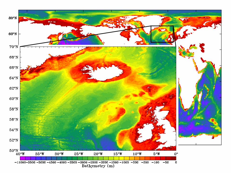
Faroe Bank Channel and Denmark Strait Outflows

Density along axis of Faroe Bank Channel

Denmark Strait: J. Girton; FBC: C. Mauritzen, J. Price

Denmark Strait Sea Surface Temperature

Abyssal Overflows – the Romanche Fracture Zone

Potential Temperature along Romanche Fracture Zone

Ferron et al., JPO 1998

Potential Temperature at 5000 m Depth

Shear instability & entrainment

Detrainment

Geostrophic eddies

xz

y

Downslope descent

Bottom friction

Physical processes in overflows

Steps in Adequately Representing Gravity Currents

1. Supply source water to the plume with the right rate and properties.

2. Model must be able to represent downslope flow without excessive numerical entrainment.

3. Parameterize entrainment & mixing to the right extent.4. Parameterize subgridscale circulations? (e.g. eddies, flow in

small channels).

Hydraulic control at sill

Bottom-stress mixing

Source water supply• Source Water properties depend on the right large-scale circulation and

properties.• Several important source waters enter through very narrow channels!

Gibraltar is ~12 km wide. Red Sea outflow channel is ~5 km wide. Faroe Bank channel is ~15 km wide at depths that matter.

Channels that are much smaller than the model grid require special treatment – e.g. partial barriers.

The topography around Gibraltar, with a 1° grid (black), and the coastline (blue) that GFDL’s 1° global isopycnal model uses.

Representing Straits with Partially Open Faces(Work with A. Adcroft, GFDL)

Partially open faces can dramatically improve simulations of overflows that pass through narrow straits.

The model equations need to be modified to be energetically consistent. E.g. Sadourny’s 1975 Energy conserving discretization of the shallow water equations:

Terms underlined in red are affected directly by using the partially open faces.

Terms underlined in blue are affected indirectly (i.e. no code changes).

uvf

hA

Aq jq

yiq

xji

h

jih

11,

,

hy

hx

hvy

vx

vuy

ux

u AAA

jvx

iuyjih

hvVhuUVUAt

h

01

j

vi

uhiu

x

ji

ux

vAuAA

MVqt

u 22

2

111

j

vi

uhjv

y

ij

vy

vAuAA

MUqt

v 22

2

111

Resolution requirements for avoiding numerical entrainment

in descending gravity currents.Z-coordinate:

Require thatAND

to avoid numerical entrainment.(Winton, et al., JPO 1998)

Suggested solutions for Z-coordinate models: "Plumbing" parameterization of downslope flow:

Beckman & Doscher (JPO 1997), Campin & Goose (Tellus 1999). Adding a separate, resolved, terrain-following boundary layer:

Gnanadesikan (~1998), Killworth & Edwards (JPO 1999), Song & Chao (JAOT 2000).

Add a nested high-resolution model in key locations? No existing scheme is entirely satisfactory!

Sigma-coordinate: Avoiding entrainment requires that

Isopycnal-coordinate: Numerical entrainment is not an issue - BUT• If resolution is inadequate, no entrainment can occur. Need

mHz BBL 502/ kmHx BBL 52/

BBLOcean HD

AmbientOverflow 21

Diapycnal Mixing Equations in Isopycnic Coordinates

• In isopycnic coordinates, diapycnal diffusion is nonlinear

• The discrete form leads to a coupled set of nonlinear differential equations

These can be solved implicitly and iteratively, with an arbitrary distribution of diffusivities to avoid the impossible time-step limit (Hallberg, MWR 2000)

• The work-diffusivity relationship is exact in density coordinates.

• Entrainment can also be parameterized directly, based upon resolved shear Richardson numbers and a reinterpretation of the Ellis & Turner (1959) bulk Richardson number parameterization (Hallberg, MWR 2000).

This parameterization gives entraining gravity currents that are qualitatively similar to observations, but has subsequently been improved upon.

z

z

t

1

11

1

11

21

21

11

k

kk

k

kk

kk

kk

k

kk

k

k

hhhht

h

8.00

8.051

8.01.0

Ri

RiRi

RiUwE

21

212

122 kkkk uuuuU

U

ghRi

gdgWork

z

hht

hwhere

212/ ht

Constant Diffusivity Richardson Number Mixing

DOME Model Intercomparisons and Resolution Dependence (Legg et al., Ocean Modelling 2006)

2.5 km x 60 m 10 km x 144 m 50 km x 144 m

10 km x 25 Layer 50 km x 25 Layer

MITgcm (Z-coordinate) with Convective Adjustment

HIM (isopycnal coordinate) with shear Ri# param.

Plume Entrainment as a Function of Resolutionfor 6 DOME Test Cases

Fin

al P

lum

e B

uoya

ncy

(m s

-2)

Ent

rain

men

t Rat

e N

ear

Sou

rce

(non

dim

.)Horizontal Grid Spacing (km) Horizontal Grid Spacing (km)

Solid lines: MITgcm (Z-coordinate)Dashed lines: HIM (Isopycnal coordinate)

For full details, see Legg et al., Ocean Modelling 2006.

Parameterizing Overflow Entrainment:Observations of Bulk Entrainment in Oceanic

and Laboratory Gravity Currents (J. Price)

A bulk entrainment law applies, provided the Reynolds number is not quite small.

Examples of Gravity Current Mixing Parameterizations:• Generic shear parameterizations – e.g. KPP (Large et al., 1994):

Typically calibrated for the Equatorial Undercurrent.

• Two-equation turbulence closures (e.g. Mellor-Yamada; k-;).• Plume-specific parameterizations – e.g. Ellison & Turner (1959) bulk Ri#

parameterization reinterpreted for shear Ri# (Hallberg, 2000):

This can be cast as a diffusivity, is over an unstable region:

8.00

8.051

8.01.0

Ri

RiRi

RiUwEntraining

22 / SNRi 32124 7.011050 Rism

Ri

Ri

Ri

g

Uo

51

8.01.0

3

May Need ResolutionDependence!

Simulated Mediterranean Outflow Plume(Papadakis et al., Ocean Modelling 2003)

Zonal Velocity

Salinity in 3 Isopycnal Layers

Salinity

A Non-rotating Overflow Entering a Stratified Environment (Courtesy T. Özgökmen)

LES and Parameterized Overflow Entrainment (Xu, Chang, Peters, Özgökmen, and Chassignet, Ocean Modelling in press)

Failure and Success of Existing Parameterizations

• A universal parameterization can have no dimensional “constants”. KPP’s interior shear mixing (Large et al., 1994) and Pacanowski and Philander

(1982) both use dimensional diffusivities.• The same parameterization should work for all significant shear-mixing.

In GFDL’s HIM-based coupled model, Hallberg (2000) gives too much mixing in the Pacific Equatorial Undercurrent or too little in the plumes with the same settings.

• To be affordable in climate models, must accommodate time steps of hours. Longer than the evolution of turbulence. Longer than the timescale for turbulence to alter its environment.

• 2-equation (e.g. Mellor-Yamada, k-, or k-) closure models may be adequate. The TKE equations are well-understood, but the second equation (length-scale,

or dissipation rate, or vorticity) tend to be ad-hoc (but fitted to observations) Need to solve the vertical columns implicitly in time for:

1. TKE2. Dissipation/vorticity3. Stratification (T & S)4. (and 5.) Shear (u & v)

Simpler sets of equations may be preferable. Many use boundary-layer length scales (e.g. Mellor-Yamada) and are not

obvious appropriate for interior shear instability.

However, sensible results are often obtained by any scheme that mixes rapidly until the Richardson number exceeds some critical value.

3-DNS of Shear Instability(L. Jackson, R. Hallberg, & S. Legg in prep.)

Kelvin-Helmholtz instability

3D stratified turbulencez

x

Tem

pera

ture

(°C

)

z

x

Tem

pera

ture

(°C

)

Temperature during initial developmentof Kelvin-Helmholtz instabilities

Representative instantaneous along-channelCross-section in statistical steady state

Considerations for a Parameterization of Stratified

Shear Instability S = ||∂U/∂z|| [s-1] Velocity shearN2 = -g/ ∂/∂z [s-2] Buoyancy FrequencyH [m] Vertical extent of small Ri

Q [m2 s-2] Turbulent kinetic energy per unit massu* = (/)1/2 [m s-1] Friction velocity (for boundary turbulence)z* [m] Distance from boundary (for boundary turbulence)

• Mixing should vanish if the shear Richardson number (Ri = N2/S2) exceeds ~1/4 everywhere

• Vigorous mixing may extend past the region of small Ri.

• Homogeneous stratified turbulence is often characterized by the buoyancy length scale

• Kelvin-Helmholtz (K-H) saturation velocity scales are ~ H S.

K-H instabilities span the region of small Ri, i.e. length scales of ~ H.

Mixing-length arguments suggest peak K-H-type diffusivities scaling as ~ H2S.

• Near solid boundaries, length scales are proportional to the distance from the boundaries, and diffusivities are ~ 0.4u*z*.

22 / NQLBuoy

The diffusion of density can be linked to entrainment parameterizations by combining the density conservation equation:

with the continuity equation in density coordinates:

The latter equality is ill-behaved when ∂/∂z=0, but with constant stratification it reduces to

)(22

2

RiFzz

u

ET parameterisation (Hallberg, 2000)

zzDt

D

Translating “Entrainment Rate” parameterizations into diffusive parameterizations (L. Jackson)

RiFzzz

zz

t zz

u

u

2

11

Properties:

• Uses a length scale which is a combination of the width of the low Ri region (where F(Ri)>0) and the buoyancy length scale LBuoy = Q1/2/N.

• Decays exponentially away from low Ri region

• Vertically uniform, unbounded limit:

• Ellison and Turner limit (large Q) reduces to form similar to ET parameterisation

• Unstratified limit: similar to law-of-the-wall theories of parabolic diffusivity between two boundaries and log-like profiles of velocity near the boundaries.

S=||Uz||

)(222

2

RiSFLz Buoy

NQLBouy /2/1

= 0 at solid boundaries

Entrainment-law derived theory for Shear-driven mixing

2BuoySL

Assumptions:

• Q reaches steady state faster than background flow is evolving so no DQ/Dt term

• Assume Pr = 1 (for now)

• Q0 needed to avoid singularity in diffusivity equation (solution not sensitive to Q0 and 0)

• Parameterization of dissipation as c(Q-Q0)N

Q intended for use in diffusivity equation is due to turbulent kinetic energy only - difficult to compare to results from DNS because of internal waves.

Dt

DQNQQcNS

z

Q

z00

220

N

QL

NL bOZ

2/1

2/3

2/1

TKE Budget to Complement Proposed Diffusivity Equation

Equilibrium DNS of Shear-driven Stratified Turbulence

• Non-hydrostatic direct numerical simulations (MITgcm)• 2m x 2m x 2.5m with grid size ~ 2.5mm in centre• Molecular viscosity and diffusivity, Kolmogorov scale mostly

resolved.• Cyclic domain in x,y• Shear and jet profiles• Statistically steady state reached • Force average velocity profiles to evolve to given profile• Initially constant stratification and relaxed to initial density

profile• All profiles are spatially averaged in x and y and time

averaged

3-DNS of Shear Instability(L. Jackson, R. Hallberg, & S. Legg in prep.)

Kelvin-Helmholtz instability

3D stratified turbulencez

x

Tem

pera

ture

(°C

)

z

x

Tem

pera

ture

(°C

)

Temperature during initial developmentof Kelvin-Helmholtz instabilities

Representative instantaneous along-channelCross-section in statistical steady state

DNS data

New parameterisation (Jackson et al.)

ET parameterisation (Hallberg 2000)

F(Ri) = 0.15*(1-Ri/0.25)/(1-0.9*Ri/0.25), c=1.9

F(Ri) = 0.15*(1-Ri/0.8)/(1+1.0*Ri/0.8), c=1.7

F(Ri) = 0.12*(1-Ri/0.25)/(1-0.9*Ri/0.25), c=1.24

DNS Shear-Instability Results and the Proposed Parameterization

Buoyancy

flux (

m2/s

3)

DNS of Shear Instability and Existing 2-equation closures

Jackson et al., proposed parameterization:

Black: DNS ResultsGreen: GOTM kBlue: GOTM kRed: Mellor-Yamata 2.5

Buoyancy

flux (

m2/s

3)

DNS Jet results

Buoyancy

flux (

m2/s

3)

DNS data

New parameterisation (Jackson et al.)

ET parameterisation (Hallberg 2000)

F(Ri) = 0.15*(1-Ri/0.25)/(1-0.9*Ri/0.25), c=1.9

F(Ri) = 0.15*(1-Ri/0.8)/(1+1.0*Ri/0.8), c=1.7

F(Ri) = 0.12*(1-Ri/0.25)/(1-0.9*Ri/0.25), c=1.24

Existing 2-equation Closures Compared to DNS Jet

Black: DNS ResultsGreen: GOTM Blue: GOTM Red: Mellor-Yamata 2.5

Jackson et al., proposed parameterizations:B

uoyancy

flux (

m2/s

3)

Dia

gnos

ed d

iapy

cnal

dif

fusi

vity

(m

2 s-1)

Gradient Richardson number

Diapycnal Diffusivities Diagnosed from 3-D DNS

Shear Instability with a Larger Ri#Not yet equilibrated?

Buoyancy

flux (

m2/s

3)

500 m x 30 m MITgcm

Ellison & Turner Mixing Only10 km x 25 layer HIM

At the start of the CPT, with thick, nonrotating plumes entering ambient stratification, GFDL’s Isopycnal coordinate model (HIM) would give plumes that split in two.

Such split plumes do not occur in nonhydrostatic “truth” simulations.

Illustrating the powerof the CPT paradigm

Observed profiles from Red Sea plume from RedSOX (H. Peters)

Well-mixedBottom BoundaryLayer

Actively mixingInterfacial Layer

Shear Ri# Param.Appropriate Here.

Bottom Boundary Layer Mixing

• Diapycnal mixing of density requires work.

• The rate at which bottom drag extracts energy from the resolved flow is straightforward to calculate.

• Assumptions: 20%? of the extracted energy is available to drive mixing. Available work decays away from the bottom with e-folding scale

of Mixing completely homogenizes the near bottom water until the

energy source is exhausted.

Legg, Hallberg, & Girton, Ocean Modelling, 2006

gdgWork 3BBLDo ucg

f

u*4.0

f

uch BBLDBBL24.0

exp2.0

500 m x 30 m MITgcm

Ellison & Turner + Drag MixingEllison & Turner Mixing Only10 km x 25 layer HIM

With thick plumes, both Interfacial andand Drag-induced Mixing are needed.(Legg et al., Ocean Modelling, 2006)

Double Mediterranean plumes without bottom-drag mixing

Year 5 salinity along 38.5°N in GFDL’s 1° Global Isopycnal Model

Adding the Legg et al. bottom-drag mixing parameterization leads to dramatic improvements in an IPCC-class ocean model.

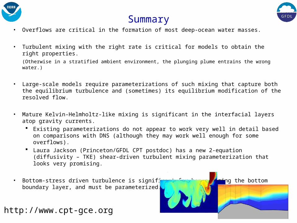
Summary• Overflows are critical in the formation of most deep-ocean water masses.

• Turbulent mixing with the right rate is critical for models to obtain the right properties.(Otherwise in a stratified ambient environment, the plunging plume entrains the wrong water.)

• Large-scale models require parameterizations of such mixing that capture both the equilibrium turbulence and (sometimes) its equilibrium modification of the resolved flow.

• Mature Kelvin-Helmholtz-like mixing is significant in the interfacial layers atop gravity currents. Existing parameterizations do not appear to work very well in detail based on

comparisons with DNS (although they may work well enough for some overflows).

Laura Jackson (Princeton/GFDL CPT postdoc) has a new 2-equation (diffusivity – TKE) shear-driven turbulent mixing parameterization that looks very promising.

• Bottom-stress driven turbulence is significant for homogenizing the bottom boundary layer, and must be parameterized.

http://www.cpt-gce.org