Embed Size (px)
Citation preview

The Effect of Restructuring on Unemployment
Andrew Figura*
Board of Governors of the Federal Reserve SystemOctober 27, 2003
JEL Classifications: E24, E32, J64
Keywords: Restructuring, Unemployment, Job Flows
Abstract: This paper finds that the permanent job losses associated with industrial restructuringhave significantly boosted the variance of unemployment, causing it to rise much higher inrecessions than it would have without cyclically correlated restructuring. Moreover, the influenceof restructuring has increased noticeably in the 1980s and 1990s, acting to increase economicinstability at a time when other factors were operating to reduce it.
*Mail Stop 80, Board of Governors of the Federal Reserve System, Washington, DC 20551. Email:[email protected]. The views presented are solely those of the author and do not necessarily representthose of the Federal Reserve Board or its staff. I would like to thank the Bruce Fallick, DougElmendorf, and Bill Wascher for useful comments.

1. Papers noting and seeking to explain the decline in the variance of GDP since the early1980s include McConnell and Perez-Quiros, 2000, Stock and Watson, 2002, and Ahmed, Levin,and Wilson, 2002.
This paper finds that changes in employment associated with industrial
restructuring have significantly boosted the variance of unemployment, causing it to rise
much higher in recessions than it would have without cyclically correlated restructuring.
Moreover, the influence of restructuring has increased noticeably in the 1980s and 1990s,
acting to increase economic instability at a time when other factors were operating to
reduce it.1 Three characteristics of restructuring have determined its effect on
unemployment. First, restructuring is not characterized by simultaneous permanent job
losses in one sector and permanent job gains in another sector within a state. Instead,
permanent job creation and permanent job destruction are negatively correlated
contemporaneously and at several lags so that an increase in permanent job loss does not
lead to new job gains either contemporaneously or in the near future. Second, changes in
permanent (or restructuring related) job flows have caused larger movements in
unemployment than other employment changes, which suggests that restructuring has
predominantly affected workers with low mobility and/or high amounts of industry
specific human capital or rents. Finally, it takes workers some time to realize that
changes in employment are permanent. This causes unemployment to rise more initially
than it would if the permanence of the change were immediately recognized.
1. Background
In this paper, restructuring is defined as the destruction and creation of job
capital, where job capital comprises the human, physical, and organizational capital
underlying particular jobs. Because much of this capital is specific to jobs, plants, or
industries (Topel, 1990, Bahk and Gort, 1993, Ramey and Shapiro, 1998), changes in
demand or technology that cause the permanent elimination of jobs destroys much of this
capital. Conversely, the building of permanent new jobs requires substantial investment
in job capital.
An example may help to clarify this idea. Suppose a manufacturer creates jobs to
make a new kind of widget. The capital behind these jobs includes: the time spent

- 2 -
2. The above process is often referred to as creative destruction, and is one process by whichnew technology becomes embodied in productive assets. New job capital is also created whenfirms upgrade technology at existing plants without creating or destroying jobs.
3. Sufficient conditions for this assumption are that restructuring occurs across and not withinplants or industries and that restructuring is caused by low frequency changes in relative demandor technology. Figura, 2003, shows that other less restrictive conditions would also be sufficient.
gathering and analyzing the information needed to decide that producing this new kind of
widget would be profitable and to determine the optimal technology to produce them; the
relationships established with both suppliers of materials needed to make the widgets and
distributors of the widgets; the machines and structures used to produce the widgets; and
the hiring and training of workers who operate the widget factory. If, at some point,
demand or technology changes so that these widgets are no longer profitable to produce
using the acquired technology, then this capital loses much of its value. The decision to
no longer produce these widgets and eliminate the jobs involved in their production in
essence destroys this capital. Finally, the process of creating and/or destroying this job
capital is what I refer to as restructuring.2 I assume that restructuring can be identified
with permanent job loss or permanent job gains.3
Because restructuring entails the destruction of built-up capital, it can have
potentially large costs, and it is in part because of these costs that it has garnered so much
attention. Much of this attention has focused on restructuring as a cause of
unemployment and a cause of rising and persistent unemployment in the last two
recessions. This paper attempts to explain what features of restructuring have led it to
affect unemployment and then attempts to quantify the importance of restructuring to
cyclical movements in unemployment.
This attempt relates to some previous research. One strand of related literature
has focused on the reallocation of workers across industries. Lilien, 1982, attempted to
measure the fraction of cyclical movements in unemployment attributable to reallocation
shocks (shocks to the optimal distribution of resources across production units) and the
fraction attributable to aggregate demand shocks. Abraham and Katz, 1986, criticized
his measure of reallocation, showing that its cyclical movements likely derived from the
different responses of sectors to aggregate shocks. Since then, much of the literature has
tried to devise better methods to distinguish between reallocation shocks and aggregate

- 3 -
4. Hall, 1970, looked at why local labor market unemployment rates differ persistently. Marsten, 1985, Bartik, 1991, and Gabriel, Shack-Marquez and Wascher, 1991, among others,examine how local unemployment rates adjust to demand shocks.
shocks as causes of cyclical movements in unemployment, Brainard and Cutler, 1993,
Campbell and Kuttner, 1996, Loungani, Rush and Tave, 1990.
This paper focuses on a different concern. Because restructuring is distinct from
other types of changes in labor demand, with different costs and potentially different
optimal public policy responses, understanding its magnitude, how it varies with the
cycle and how workers affected by it respond are important questions, regardless of
whether cyclical movements in restructuring are exogenous or driven by aggregate
demand shocks. Instead of trying to discern the origins of cyclical movements in
restructuring, this paper asks the following questions: has unemployment caused by
restructuring been different than unemployment caused by temporary demand or supply
shocks, what is the share of aggregate unemployment changes due to restructuring, and
has this share changed over time.
The correlation between restructuring and the business cycle prevents
identification of both the causes and effects of restructuring at the aggregate level. In an
attempt to identify the effects, I follow another strain in the literature, which exploits
heterogeneity in regional, state, and local labor markets.4 Though restructuring related
job flows are correlated with the cycle, they occur at differing magnitudes at different
times in different states. For example, Michigan in the early 1980s had above average
restructuring related to problems in the domestic auto industry, while California in the
early 1990s had a relatively large amount of restructuring related to defense cutbacks
following the end of the Cold War. This variation helps to identify the effect of
restructuring on unemployment.
Some previous papers have looked at the effects of different types of shocks on
local unemployment (Holzer, 1991, Bound and Holzer, 2000, and Loungani and Bharat,
1997), while other papers have examined local labor force responses to different types of
shocks (Bound and Holzer, 2000, and Topel, 1986). However, none have measured the
effects of industrial restructuring on unemployment, examined how labor force responses
to industrial restructuring differ from other types of labor demand shocks, nor looked at

- 4 -
5. Groshen and Potter (2003) investigate whether restructuring has changed over time.
6. With some minor modifications, which would not affect the main results, shocks could alsorepresent changes in the relative demand for the output of a segment.
the cyclical variation of industrial restructuring and how its influence on unemployment
has changed over time.5
2. Modeling Restructuring and Changes in State Unemployment
Model
The basic model derives from Lucas and Prescott, 1974. In the model there are
many labor market segments, where workers can produce either market or non-market
goods. The technology for market output is subject to random shocks, which cause
workers to move into and out of unemployment within a labor market segment and to
move across labor market segments.6 Because longer lasting shocks to market output
technology (those related to restructuring) have greater effects on the value of being in a
particular labor market, they produce larger movements in the labor force, and as a result,
smaller movements in unemployment. However, this prediction can be modified in two
ways. First, if workers are initially unsure if a change is long-lasting, the labor force
movements caused by restructuring may be delayed. Second, if restructuring tends to
affect segments where workers are less mobile or if restructuring is positively correlated
among segments where mobility is easiest, the relative effect of restructuring on
unemployment becomes ambiguous.
Job market segments are indexed by i, i=1 to M. There are an infinite number of
workers distributed on the interval [0,1] and indexed by j. In time period t, a worker in
segment i can pursue one of three activities: produce market output, yi, and be employed,
produce non-market output, h, or move to a different labor market segment. In the latter
two activities, workers are considered to be unemployed.
The technology for market production, yi, is
(1)y f ei t i t i t, , ,( , )= α
where ei,t is employment in segment i at time t and "i,t is the parameter governing
technology in segment i. The market production technology has the following attributes
- 5 -
(2)f e f e f e f ei t i t e i t i t ee i t i t ea i t i tα α α α α( , ) , ( , ) , ( , ) , ( , ), , , , , , , ,> > < >0 0 0 0
where subscripts on f denote derivatives.
Non-market production technology is
(3)h l= χ
Workers must devote their time wholly to market or non-market production
(4)e l e l, ( , ),∈ + =0 1 1
The labor force in segment i, lfi,t, equals the number of workers in segment i;
employment, ei,t, equals the number of workers employed in segment i; and
unemployment is the difference between the two
(5)lf jdj e e dj u lf ei tj i
i t j tj i
i t i t i t, , , , , ,, ,= = = −∈ ∈∫ ∫
Utility is linear in the consumption of market and non-market goods.
(6)u y h y hi t i t( , ), ,= +
At the start of period t, shocks to each segment’s relative technology are realized,
and workers in each segment choose whether to remain in the segment or move to
another segment. If they remain in the segment, they must choose whether to produce
market output and be employed or produce non-market output and be unemployed. If
agents choose to move, they must acquire new skills and search for a job. As a result,
they must spend a period producing neither market nor non-market output.
First, consider the decision to produce market or non-market output. From (1)-
(6), workers in a segment will produce market goods until the marginal utility of market
production equals the marginal utility of non-market production.
(7)f ee i t i t( , ), ,α χ=
However, the beginning period labor force may constrain the amount of
employment, so that
(8)f e Max f lfe i t i t e i t i t( , ) ( , ( , )), , , ,α χ α=

- 6 -
Next, consider the decision whether to remain in segment i or move to another labor
market segment. At the beginning of period t, the value of remaining in segment i,
assuming no change in the labor force, is
(9)( )V lf Max f lf EV lfi ti t i t e i t i t
i ti t i t
,, , , ,
,, ,( , ) ( , ), ( , )α α χ β α− −
++ −= +1 1
11 1
If workers move they receive .{ }β α λE Max V lf Ek
k tk t k t t
,, ,( , )++ − =1
1 1
In equilibrium workers should move to segments with the highest expected future
value, and the value of segments which receive new workers should be equal. So for any
segment i that receives workers, i0R, the values should be equal and greater than any
other segment.
(10)E EV lf EV lf EV lf i j R k Rt i t i t j t j t k t k tλ β α β α β α= = ≥ ∀ ∈ ∀ ∉+ + +( , ) ( , ) ( , ), , ,, ,*
, ,*
, ,*
1 1 1
where is the equilibrium value of the labor force in segment k at the end of period t,lf k t,*
and 8t represents the value of moving out of a segment. In equilibrium, the value of
being in segment i is
(11)( ) { }{ }V lf Max Max f lf EMin V lfi t i t e i t i t i t i t t ti t( , ) ( , ), ( , ), ,, , , , , ,
*,
α α χ β α λ λ− − += +1 1 1
The ability to move across segments insures that there is a floor under the value
of being in segment i equal to E8t and a ceiling equal to
(12)( )Max f lf Ee i t i t ti tχ α λ, ( , )
, , , +
Unemployment occurs in segment k when (7) holds and
(13)χ β α λ+ ≥++EV lf Ei t
i t i t t,
, ,*( , )1
1
or when the segment increases its labor force, . In the former case,lf lfi t i t,*
,*> −1
unemployment occurs because the value of non-market production exceeds the value of
market production when the entire labor force is employed, but outside opportunities are
not attractive enough for all non-employed workers to leave. In the latter case, workers
are unemployed because they must spend a period acquiring skills and searching for jobs
when they first enter a labor market segment.
- 7 -
7. In Mortensen and Pissarides, 1994, building new job capital is accomplished by job search,while in Caballero and Hammour, 1996, building job capital also entails some sunk costs. As aresult, job destruction is countercyclical, while job creation is procyclical. For the present modelto match the procyclical nature of job creation, some friction in the job creation process wouldneed to be introduced.
This model has the feature that given some reasonable assumptions (see proof (i)
in Appendix) restructuring occurs in downturns. To see this, suppose that "i has a
component common to all segments, and an idiosyncratic component, specific to each
segment and independent across segments.
(14)α α αi t t i t, ,$ ~= +
One could think of movements in the common component, , as aggregate technology$α
shocks. Given (7) and , workers are more likely to be employed when is high. fα > 0 $α
However, when declines, production of market goods becomes less attractive relative$α
to non-market production and moving across sectors. More formally, at the beginning of
a period, agents move out of a segment when the cost, , is less( )Max f lfe i t i ti t,( , ),, ,α χ−1
than the benefit, . Differentiation of these values shows that( )E V lfti t
i t i tλ β α− ++ −
,, ,( , )1
1 1
the cost is more procyclical than the benefit, causing movement across sectors to be
countercyclical. If the difference in values between segment i and the best alternative is
permanent, then this movement represents restructuring. This implication of the model is
similar to Davis and Haltiwanger, 1990, Mortensen and Pissarides, 1994, and Caballero
and Hammour, 1996.7
Now, consider the effect of long-duration versus short duration changes in
demand. Suppose " has natural value and that " can only deviate from this value forα
specific durations, n1 and n2, where n1>n2. In any period in which , there is aα α=
probability, (, that " changes. . With probability By the change is long-∆α σ~ . . .( , )i i d 0
duration and with probability (1-By) it is short-duration. For example, if "i,t+1>"i,t, and
this is a long-term change, then and . Then,α α α αi t i t i t i t n, , , ,...+ + + += = = =1 2 3 1α αi t n, + + =
1 1
assuming that labor force flows occur for both permanent and temporary changes in

- 8 -
demand, from and equation (11), a long duration change in " will cause a∂∂αV i t
i t
,
,
> 0
larger movement of the labor force either into or out of segment i then a short duration
change in ", as in Topel, 1986 (see proof (ii) in the Appendix).
With the existence of unemployment in segment i, equation (7) holds, and the
change in employment in period t just depends on the change in "i,t, not its duration. As a
result, the change in employment caused by either the short or the long duration
movement in " is the same. Then since the change in unemployment in segment i is
(15)∆ ∆ ∆ ∆u elf lf ei t
i t
i ti t i t,
,
,, ,ln ln( ) ln( )≈ −
= −
the unemployment rate will change less with a longer duration or permanent change in
demand than with a short duration change.
This result can be modified in two ways: first, if agents are uncertain whether a
change in " is short-duration, event s, or long duration, event l; second, if permanent
changes tend to affect sectors where it is costly to move or if permanent changes are
positively correlated among sectors where mobility is relatively costless.
If agents are uncertain whether a change in " is short-duration or long duration,
they may delay movement, and the initial effect of a permanent change may be very close
to a non-permanent change in demand. With time, however, as the duration of the
change increases, agents will increase their subjective probabilities that the shock is
permanent and act accordingly. Given the unconditional probabilities of short duration,
(1-Bx), and long duration, Bx, employment changes, if the change in "i has lasted g
periods, by Bayes’ Law, the conditional probability that it is a long-term change is
(16)Pr( | ) Pr( | )Pr( | )( ) Pr( | | )
∆∆
∆ ∆α α π
α π α πii x
i x i x
l d g d g ld g s d g l
= = == =
= = − + = =1
where d is the duration of )"i. If , then as∂ α
∂∂ α
∂Pr( | ) Pr( | )d g s
gd g l
gi i= =
<= =∆ ∆
the duration increases, agents will come to assign more probability weight to a long-
duration shock. Thus, initially, if workers have relatively little information about the

- 9 -
duration of a shock, they may respond similarly to short-term and long-term shocks, but
over time, as they accumulate knowledge, movements out of the labor force should be
greater for long-term shocks (see proof (iii) in the Appendix).
Next, suppose there are fixed costs of moving out of sector i, Ci. Then equation
(11) becomes
(17)( ) { }{ }V lf Max Max f lf EMin V lf Ci t i t e i t i t i t i t t ti t( , ) ( , ), ( , ), ,, , , , , ,
*,
α α χ β α λ λ− − += + −1 1 1
As a result, labor force movements in response to changes in " are smaller in segments
with higher fixed costs. When " decreases, agents hesitate to move out of the segment
because of the high cost involved. When " increases, agents hesitate to move in,
knowing that if they need to subsequently leave, the cost will be high. With smaller
changes in the labor force, but the same movement in employment, fluctuations in
unemployment are larger for high cost sectors (see proof (iv) in the Appendix). If
permanent changes tend to be concentrated in high cost sectors, then the unconditional
correlation (i.e. not conditioning on mobility costs) between restructuring and
unemployment will be of ambiguous value relative to the unconditional correlation
between other employment changes and unemployment.
There are a couple of reasons why restructuring may be concentrated in high
mobility cost segments. First, restructuring may be more likely to affect workers earning
rents, who may be less likely to move in response to layoffs. In the context of the model,
leaving a segment forces a worker to forego these rents, and the present value of this loss
is Ci. Summers, 1986, shows that workers in sectors with high unionization, such as the
auto and steel industries, have wages higher than similar workers elsewhere, and that
declines in employment in these industries tend to cause larger movements in
unemployment. Given a trend toward greater international economic integration and
hence greater competition for many industries, one would also predict that industries with
high rents would be the most likely to undergo restructuring.
Second, restructuring may be more likely to affect workers with relatively large
amounts of segment specific capital. Fallick, 1993, shows that unemployed workers with
large amounts of specific human capital are less likely to leave their sector to find
employment. In the context of the model, the present discounted value of the difference
- 10 -
in earnings between the segment where workers have significant amounts of human
capital and other segments is Ci. Oi, 1962, shows that firms should concentrate
temporary cyclical layoffs among workers with less firm specific human capital. If
permanent changes in employment force firms to make deeper cuts in their work forces
or force them to hire skilled, as well as marginal employees, restructuring should affect a
higher proportion of workers with large amounts of human segment specific capital. In
support of this, plant births and deaths, which destroy all jobs at a plant, not just marginal
jobs, represent a significant share of total permanent changes in employment in the
manufacturing sector (Figura, 2002).
Permanent changes in demand may also have larger effects on unemployment if
they are positively correlated across sectors between which the cost of moving is low.
Suppose that some segments are more similar to each other than other segments. For
example, assume that there are s labor market divisions, where M/s is an integer greater
than 1 and less than M. To move across divisions, workers must pay a fixed cost, C, but
within a division there is no fixed cost for movement between labor market segments.
Then changes in technology across segments will have larger effects on unemployment if
these changes are positively correlated within divisions. If divisions with adverse
relative technology shocks are also divisions with beneficial relative shocks, then
unemployment movements within a division will be small. However, when divisions
with a relatively large number of adverse shocks are also divisions where there are a
relatively small number of beneficial changes, then the change in unemployment will be
larger. Thus, if restructuring tends to be positively correlated among segments where
mobility is relatively costless, then it can have a larger effect on unemployment than
other employment changes (see proof (v) in the Appendix).
Juhn, Murphy and Topel (1991) exemplify a large body of research, which finds
that unemployment has risen disproportionately among low-wage or low-skill workers
and attributes the rise to an adverse shift in the demand for unskilled labor. The relative
rise in unemployment for low-skill workers has been long-lasting and the adverse
demand shift against low-skilled labor has been strongly positively correlated across jobs
employing low skill workers. Thus, the opportunities for a low-skill worker to move to a
better job when her own job has suffered an adverse demand shock have been reduced
- 11 -
because jobs to which it is relatively costless (requiring little skill up-grading) to move
have also suffered adverse shocks.
Estimating Equation
To estimate the effect of restructuring on unemployment I start with equation (15)
which relates changes in unemployment to changes in employment and the labor force.
Then I use the fact that changes in employment can be decomposed into permanent and
temporary job creation and permanent and temporary job destruction
(18)∆ ∆ ∆
∆ ∆
ln ln( ) ln( )ln( ) , ln( )
, , ,
, , , , , ,
e ep etep pjc pjd et tjc tjds t s t s t
s t s t s t s t s t s t
= +
≈ − ≈ −
where )ln(e) is the log difference in employment, ep is permanent employment, et is
temporary employment, pjc is permanent job creation and pjd is permanent job
destruction.
Next, equation (19) models changes in the labor force as caused by previous
changes in unemployment (the discouraged worker effect) plus the pattern of recent job
flows, which accounts for the potential differences in labor force movements caused by
permanent and temporary employment changes. In addition, there may be unobserved
factors that cause variations in the labor force. These factors are accounted for in
equation (19) if they are constant across time but vary across states or if they are common
across states but vary across time.
(19)( )
, , 1 , ,
,
,1 2 3 4,
,
,
ln ( ) ( )
;
s t s t s t s t s t
s t
s ti i i i i s t
s t
s t
lf L u L JF
pjcpjd
JFtjctjd
α θ β ε
γ γ γ γ
−∆ = + + ∆ + Γ +
Γ = =
$(L) and '(L) represent polynomial distributed lags. Combining (15), (18) and (19)
yields my estimating equation (20)
(20)∆ ∆ Ψ
Ψ Γ Ψ Γ
u L u L JFi i i d
s t s t s t s t s t
i i s t
, , , ,
,
( ) ( ), , ; ~ . . .
= + + + +
= − = ≠−α θ β εε
1
0 0 1 0
- 12 -
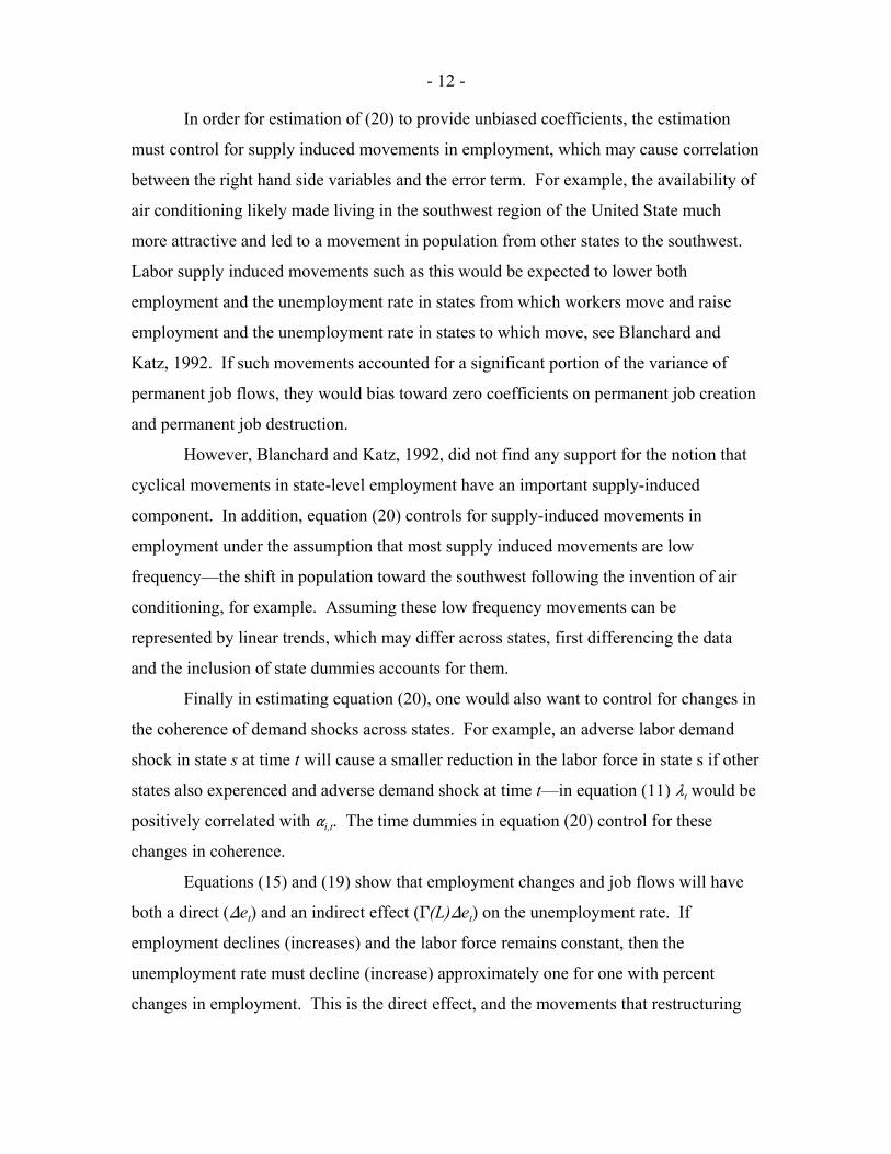
In order for estimation of (20) to provide unbiased coefficients, the estimation
must control for supply induced movements in employment, which may cause correlation
between the right hand side variables and the error term. For example, the availability of
air conditioning likely made living in the southwest region of the United State much
more attractive and led to a movement in population from other states to the southwest.
Labor supply induced movements such as this would be expected to lower both
employment and the unemployment rate in states from which workers move and raise
employment and the unemployment rate in states to which move, see Blanchard and
Katz, 1992. If such movements accounted for a significant portion of the variance of
permanent job flows, they would bias toward zero coefficients on permanent job creation
and permanent job destruction.
However, Blanchard and Katz, 1992, did not find any support for the notion that
cyclical movements in state-level employment have an important supply-induced
component. In addition, equation (20) controls for supply-induced movements in
employment under the assumption that most supply induced movements are low
frequency—the shift in population toward the southwest following the invention of air
conditioning, for example. Assuming these low frequency movements can be
represented by linear trends, which may differ across states, first differencing the data
and the inclusion of state dummies accounts for them.
Finally in estimating equation (20), one would also want to control for changes in
the coherence of demand shocks across states. For example, an adverse labor demand
shock in state s at time t will cause a smaller reduction in the labor force in state s if other
states also experenced and adverse demand shock at time t—in equation (11) 8t would be
positively correlated with "i,t. The time dummies in equation (20) control for these
changes in coherence.
Equations (15) and (19) show that employment changes and job flows will have
both a direct ()et) and an indirect effect ('(L))et) on the unemployment rate. If
employment declines (increases) and the labor force remains constant, then the
unemployment rate must decline (increase) approximately one for one with percent
changes in employment. This is the direct effect, and the movements that restructuring

- 13 -
imparts to unemployment via this effect are governed by the time series properties of
permanent job flows.
In addition, to the direct effect of job flows on unemployment, there is an indirect
effect arising from the fact that some workers flowing into and out of employment may
exit the labor force instead of entering unemployment, or some non-employed workers
may react to a change in job flows by dropping out of or entering the labor force. Given
a direct effect of 1 for a change in employment, the indirect effect will be ,γ ij
i∑ −1
j=1,2,3,4.
3. Data
Sources
The unemployment rate data are from a data set used by Blanchard and Katz
(1992) and made available by the BLS. It has annual observations on unemployment in
each state and the District of Columbia from 1976-2000. In addition, data on 27 states
are available back to 1970. The data derive from annual averages of measures of
unemployment from the Current Population Survey. Data on job flows come from the
BLS’ Current Employment Statistics (CES). The CES data cover a long time period,
1939-present, but its industry detail is limited to one-digit SIC. While the CES is a
sample survey covering approximately 30-40 percent of employment, it is benchmarked
annually to Unemployment Insurance records, and thus at annual frequencies, the data
provide a near universal accounting of state-level employment.
Defining Permanent and Temporary Employment movements
Under some reasonable assumptions discussed in Figura (2003), restructuring can
be measured using permanent changes in employment. To measure permanent changes, I
apply a low pass filter to time series of state/industry level employment. The filter is a
symmetric backward and forward weighted moving average of state/industry
employment, with weights chosen to isolate particular frequencies of employment
movements, see Baxter and King, 1999. I identify restructuring as long-term or
persistent movements in employment. Thus, if an industry loses 1,000 jobs and this job

- 14 -
8. Temporary state/industry-level job flows may contain permanent plant-level job flows ifone set of plants destroys jobs permanently, and soon afterwards another set of plants within thesame state/industry creates jobs permanently. Davis, Haltiwanger and Schuh (1996) show that forthe manufacturing sector the level of industry job flows is considerably smaller than the level ofplant-level job flows. However, Figura (2002) shows that the cyclical variation in plant-levelpermanent job flows is well captured by movements in industry-level permanent job flows. Thus,changes in aggregate restructuring using state/industry-level data should follow closely changesin aggregate restructuring measured by plant-level data.
9. See, for example, Stock and Watson (1999).
10. More specifically, the job flows used for the right hand side of equation (20) are theaverage of the twelve year-to-year monthly job flows. This corresponds to the change in annualunemployment being the average of the twelve year-to-year monthly changes.
loss persists for some time, I attribute the job loss to restructuring. If, instead, job losses
are followed soon afterwards by job gains, I attribute these movements to cyclical
demand fluctuations. I make an analogous distinction for job creation.8
In implementing the filter, one must choose a cut-off date to separate persistent
low frequency movements from high frequency changes. Consistent with much of the
literature, I use 8 years to separate cyclical employment changes from secular
movements.9 A noticeable feature of the low pass filter is that it smooths the permanent
component, such that permanent changes are assumed to be slow and drawn out. Figure
1 illustrates this by decomposing manufacturing employment in Michigan into permanent
and temporary components. If the pattern of permanent changes is more abrupt than
assumed by the filter, problems could arise when estimating the effects of permanent
changes. I address this concern in the next section.
One can decompose permanent employment movements into permanent job
creation and permanent job destruction. I construct permanent job flows at the industry
level similarly to job flows constructed at the plant level by Davis, Haltiwanger and
Schuh (1996). An industry has non-zero permanent job destruction at time t if permanent
employment in the industry has decreased from t-1 to t, and non-zero permanent job
creation if permanent employment in the industry has increased from t-1 to t. Aggregate
permanent job creation (destruction) is the sum of all industry-level permanent job
creation (destruction) in state s at time t. To transform flows into rates, I divide by the
average of total state-level employment in t-1 and t.10

- 15 -
10. (...continued)
u u u u u uyear year monthmonth
year year year monthmonth
year month= − = −=
−=
−∑ ∑112
1121
12
11
12
1, , ,, ( )
Characterizing Permanent Job Flows
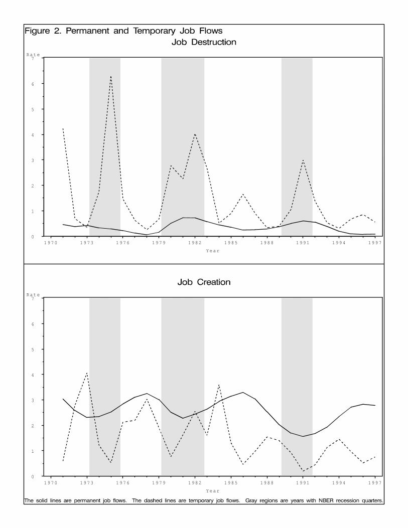
Before turning to estimation results, it is instructive to consider some
characteristics of permanent job flows. Figure 2 graphs time series of permanent and
temporary job flows. The correlation between permanent employment movements and
temporary movements, 0.33, is positive, and from figure 2 the comovement between
permanent and temporary job flows appears to be greater during recessions. There is
some variation across recessions in the ratio of permanent to temporary job flows, with
the recessions in the early 1980s and 1990s having relatively more permanent job
destruction than the 1974-75 recession. But with just three recessions, it would be quite
difficult with aggregate data to distinguish the effects on unemployment of structural
versus cyclical employment changes.
Table 1. Permanent Job Flow Variation Across Regions and Decades
Job Destruction Ratio Job Creation Ratio
Region 1971-1979
1980-1989
1990-1998
1970-1998
1971-1979
1980-1989
1990-1998
1970-1998
Pacific1 0.02 0.08 0.34 0.13 1.86 2.64 2.87 2.28
Mountain 0.01 0.18 0.04 0.09 2.08 1.73 4.04 2.29
WN Central 0.05 0.19 0.05 0.11 1.42 1.44 2.89 1.70
WS Central 0.00 0.37 0.08 0.19 2.98 1.22 3.59 2.33
EN Central 0.15 0.42 0.08 0.23 0.81 1.31 2.54 1.24
ES Central 0.02 0.22 0.13 0.11 1.21 1.64 2.90 1.64
New England 0.18 0.19 0.71 0.28 1.04 1.20 1.67 1.21
Mid Atlantic 0.49 0.70 0.70 0.61 0.86 1.94 2.08 1.47
South Atlantic 0.08 0.10 0.21 0.11 1.41 2.16 3.21 1.98
1. Excludes Alaska and Hawaii. Note. The job destruction ration is the average of permanent job destruction divided by theaverage of temporary job destruction. The job creation ratio is defined analogously.

- 16 -
However, table 1 breaks down the ratio of permanent to temporary job flows by
region and by decade and shows that there is considerable variation in the amount of
restructuring across states and across time. For example, the 1980s were particularly
severe, in terms of permanent job destruction, for the East North Central region, where
much of the auto and steel industries was concentrated, and for the West South Central
region. In contrast, for the Pacific region, the 1980s was relatively benign, but the region
was hit hard during the 1990s. Thus, conditioning on the total amount of job destruction
occurring, if permanent job destruction causes greater (smaller) increases in
unemployment than other kinds of job destruction, one would expect larger (smaller)
increases in unemployment in the 1980s in the East North Central region than in the
Pacific region. The relative unemployment experiences would then be reversed in the
1990s.
Table 2. Job Flows by Industry
AVERAGE RATES TOTAL JOBS (1970-98)1
Industry PJD PJC TJD TJC PJD PJC TJD TJC
Mining 2.6 2.2 4.5 4.8 558 516 1097 1088
Construction 1.0 3.1 3.6 3.9 1226 3906 4434 4436
Manufacturing 0.8 0.7 1.7 1.9 4798 3845 10487 10034
TPU 0.2 1.6 1.2 1.2 259 2548 1884 1810
Trade 0.1 2.4 0.9 1.0 410 15125 6067 5866
FIRE 0.1 2.5 0.9 0.9 180 4013 1464 1563
Services 0.0 4.7 1.1 1.1 0 27882 6456 6409
1. In thousands.
Table 2 shows the industry breakdown of permanent and temporary job flows. As
one would expect, the highest rates of temporary job creation, tjc, and temporary job
destruction, tjd, occur in the more cyclically sensitive goods producing industries.
Unsurprisingly, the largest destroyer of permanent jobs over the 29 years from 1970 to
1998 has been the manufacturing sector, though the smaller mining and construction
sectors have had larger rates of permanent job destruction on average. Permanent job

- 17 -
destruction in the retail and wholesale trade industry has been negligible, while in the
services industry it has been nonexistent. Services and trade have created the most
permanent jobs since 1970, though all sectors, including those with large amounts of
permanent job destruction, have created a significant number of permanent jobs. For
example, the manufacturing sector has created nearly four million permanent jobs since
1970.
4. Results
Direct Effect of Restructuring on Unemployment
From equations (15) and (18) the change in unemployment caused by the direct
effect of restructuring, )up, is
(21)∆ ∆u eps tp
s t, ,ln( )=
Thus, one can decompose the standard deviation of the change in unemployment due to
the direct effect into a restructuring term a non-restructuring term and a covariance term.
Under this calculation, restructuring accounts for about one-quarter of the variation in the
change in unemployment, other employment changes account for about three-fifths, with
the covariance term accounting for the remainder.
However, because , the variance of us,t conditional on us,0,u u us t s s mm
t
, , ,= +=∑0
1
∆
VAR(us,t)|us,0=u, depends on the variance and autocovariances of )us,t.
(22)( )Var u u uVar u u u
Cov u u u us t s
s ii
t
s
j ii
t
s i s j s
, ,
, ,
, , ,
|( | )
( , | )0
10
02= =
= +
=
=
>
∑
∑∑
∆
∆ ∆
Lines 1 and 2 of table 3 shows that covariances of permanent employment
changes are much larger than for other employment changes. Thus, the direct effect of
restructuring on the variation in unemployment is greater than its influence on the change
in unemployment. Unlike temporary changes in employment, permanent employment
changes in an industry do not have to engender permanent changes in the opposite
- 18 -
11. This point is similar to that made in Blanchard and Katz, 1992. However, as Hall, 1992,pointed out in his discussion of that paper, that result followed directly from Blanchard andKatz’s definition of permanent employment changes. Under the definition of industrialrestructuring in this paper, permanent job changes in one industry within a state can engenderpermanent job changes of equal magnitude and of opposite direction in the future. Thus,permanent changes at the industry level do not necessarily lead to permanent changes inemployment at the state level and the need for net migration. That they do is an empirical result.
12. Because by the construction of the low-pass filter individual industry/state permanent jobflows are more persistent, the relatively larger autocovariances of permanent employmentchanges may seem at first uninteresting. But permanent employment changes at the state-levelinvolve the summing of individual industries; consequently, as shown below, average state-levelautocovariances depend on the correlations of permanent employment changes across industries,as well as individual industry autocovariances.
(24)( ) ( ) ( ), , , ,, , ,t t i j t j t i j t m t ij j j m
E ep ep E ep ep E ep ep− − −≠
∆ ∆ = ∆ ∆ + ∆ ∆∑ ∑∑In fact, about 95 percent of the dynamic correlations of permanent employment are accounted forby dynamic covariances across rather than within industries within states.
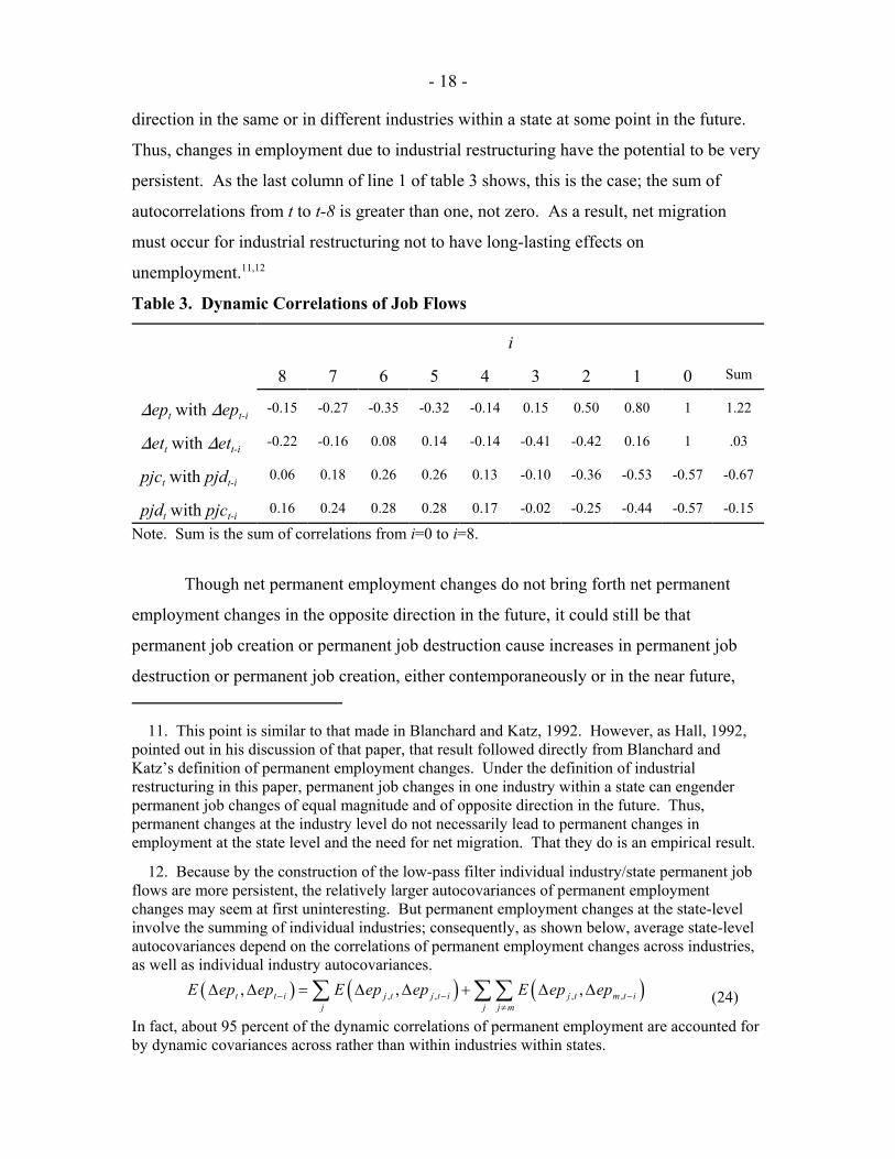
direction in the same or in different industries within a state at some point in the future.
Thus, changes in employment due to industrial restructuring have the potential to be very
persistent. As the last column of line 1 of table 3 shows, this is the case; the sum of
autocorrelations from t to t-8 is greater than one, not zero. As a result, net migration
must occur for industrial restructuring not to have long-lasting effects on
unemployment.11,12
Table 3. Dynamic Correlations of Job Flows
i
8 7 6 5 4 3 2 1 0 Sum
)ept with )ept-i -0.15 -0.27 -0.35 -0.32 -0.14 0.15 0.50 0.80 1 1.22
)ett with )ett-i -0.22 -0.16 0.08 0.14 -0.14 -0.41 -0.42 0.16 1 .03
pjct with pjdt-i 0.06 0.18 0.26 0.26 0.13 -0.10 -0.36 -0.53 -0.57 -0.67
pjdt with pjct-i 0.16 0.24 0.28 0.28 0.17 -0.02 -0.25 -0.44 -0.57 -0.15
Note. Sum is the sum of correlations from i=0 to i=8.
Though net permanent employment changes do not bring forth net permanent
employment changes in the opposite direction in the future, it could still be that
permanent job creation or permanent job destruction cause increases in permanent job
destruction or permanent job creation, either contemporaneously or in the near future,

- 19 -
just not in sufficient magnitude to prevent a net change in permanent employment. Lines
3 and 4 of table 3 shows that this is not the case. Permanent job creation and permanent
job destruction are, in fact, negatively correlated contemporaneously and at leads and
lags of one and two years. Thus, restructuring in one industry is not mitigated by
increased hiring in a different industry within a state; instead the decline in the state job
market is amplified by reduced job creation in other industries.
The results for net permanent employment changes may also mask important
differences between how state economies react to increases in permanent job destruction
and permanent job creation. Lines 3 and 4 of table 3 show that neither permanent job
destruction nor permanent job creation brings forth sufficient amounts of permanent
employment changes in the opposite direction to prevent net permanent employment
from changing. However, it appears that reversion in permanent employment changes is
stronger for permanent job creation, implying that permanent job destruction may lead to
more persistent changes in unemployment.
Table 4. Average State level Correlations between Job Flows
Correlation Between 1971-1979 1980-1989 1990-1998 1971-1998
Permanent Job Creation andPermanent Job Destruction
-0.31(0.03)
-0.36(0.01)
-0.61(<0.01)
-0.19(0.18)
Note. Significance levels (the probability that the correlation equals zero) are reported inparentheses.
Table 4 offers a different look at the relationship between permanent job creation
and permanent job destruction within a state. It reports the correlation across states of
average permanent job creation and average permanent job destruction. For the full
sample the correlation is negative, but significant only at the twenty percent level.
However, for the two most recent decades, the correlation has grown more negative and
was significant at the one percent level in both the 1980s and the 1990s. The implication
is that states that destroy a lot of jobs are not states that create a lot of jobs.
The above analysis suggests that permanent job destruction does not lead to
permanent job creation. Therefore, unless there is greater mobility in response to
restructuring-related changes in employment, restructuring will lead to more persistent
movements in unemployment than other kinds of employment changes.

- 20 -
13. Lagged dependent variables produce biased coefficient estimates when the time dimensionis limited. However, because of the relatively large time dimension and the a priori expectednegative coefficients on lagged unemployment, the bias imparted is likely trivial, Hsiao (1989).
Total Effect of Restructuring on Unemployment
The total effect of restructuring on unemployment can be seen in table 5, which
reports results from the estimation of (20). I use two lags in the polynomials on job flows
and two lags of the dependent variable.13 Observations are weighted by the level of
employment in the state in the relevant year. The first column of the table shows
estimates using net changes in permanent and temporary employment (the coefficients on
permanent job creation and permanent job destruction are constrained to be equal in
absolute value and opposite in sign), while the second column decomposes each type of
employment movement into a job creation and a job destruction component.
Three features of the estimated coefficients are of particular interest. First,
permanent movements in employment cause a larger initial effect on unemployment than
temporary movements. Second, lagged permanent employment movements also have a
bigger effect on unemployment than lagged temporary employment changes, though in
the opposite direction. Lastly, permanent job destruction has a bigger and more lasting
impact on unemployment than permanent job creation.
The absolute value of the coefficient on permanent employment changes in
column 1, 0.60, is six times larger than the absolute value of the coefficient on temporary
changes. If structural changes affected the same types of workers as other employment
changes, one would expect the coefficient on permanent changes in employment to be
smaller in absolute value than the coefficient on temporary changes. Thus, structural
shocks must have affected workers who were more immobile than other workers. The
reason for their immobility is not apparent, but from the discussion above, plausible
explanations are that structural changes have involved an adverse broad-based shift in the
demand for low-skill workers and/or have disproportionately caused the destruction of
jobs with substantial rents or with large amounts of job specific human capital.

- 21 -
Table 5. Estimation Results
Annual Triennial(1) (2) (3)
)u(-1) -0.14(0.03)
-0.25(0.03)
-0.23(0.04)
)u(-2) -0.09(0.03)
-0.24(0.03)
PJC -0.60(0.07)
-0.40(0.06)
-0.18(0.02)
PJD 0.60(0.07)
0.67(0.13)
0.61(0.05)
TJC -0.10(0.01)
0.05(0.01)
0.01(0.03)
TJD 0.10(0.01)
0.34(0.02)
0.15(0.03)
PJC(-1) 0.51(0.13)
0.16(0.09)
0.09(0.02)
PJD(-1) -0.51(0.13)
0.28(0.22)
-0.16(0.05)
TJC(-1) -0.03(0.01)
-0.04(0.01)
-0.05(0.03)
TJD(-1) 0.03(0.01)
-0.12(0.03)
-0.01(0.03)
PJC(-2) -0.08(0.07)
0.09(0.05)
PJD(-2) 0.08(0.07)
-0.47(0.13)
TJC(-2) -0.01(0.01)
-0.01(0.01)
TJD(-2) 0.01(0.01)
-0.06(0.02)
R2 0.76 0.81 0.90Note. Column (1) imposes the constraints that the coefficients on job creation are equal thenegative of the coefficients on job destruction. All regressions include state fixed effects and yeardummies. Standard errors are in parentheses.
The coefficients on lagged permanent employment changes are significantly
different from zero and are opposite in sign to contemporaneous coefficients of
permanent employment changes. According to the model, this can occur if workers do

- 22 -
not initially realize that structural changes are permanent; but as they realize the true
duration of the shock (after a year), they react accordingly.
The second column of table 5 shows coefficients on the two components of
restructuring, permanent job creation and permanent job destruction. The hypotheses
that coefficients for permanent job creation and job destruction are equal, as well as that
coefficients on temporary job creation and job destruction are equal, can be rejected at
the one percent level of significance. Permanent job destruction has a larger initial
impact than permanent job creation on unemployment. Moreover, even after two years
the net effect of permanent job destruction, as computed by the sum of the
contemporaneous and lagged coefficients, is significantly different from zero and
significantly larger than the effect of permanent job creation. Apparently permanent job
destruction has disproportionately affected immobile workers, and even after two years,
migration or withdrawals from the labor force have not eliminated the effects of
permanent job destruction on unemployment. This is not surprising, given that the
explanations offered above for why permanent changes in employment might affect
unemployment more than temporary changes appear more relevant for permanent job
destruction than for permanent job creation.
Robustness
(i) Parameterizing labor supply induced employment movements
As discussed in section 2, identification of parameters requires that employment
movements related to changes in labor supply be controlled for. Section 2 discussed the
conditions under which estimation of equation (20) is unbiased: low frequency labor
supply movements can be represented by a constant trend within each state. Another
plausible representation is a slowly evolving trend within each state. To test this
hypothesis, I include a time trend interacted with state dummies, which allows
employment caused by labor supply movements to vary quadratically within each state
across time. Estimation results are qualitatively similar to those in table 5, and an F test
of the joint hypothesis that all year/state interactions are zero cannot be rejected at a very
high level of confidence.
- 23 -
14. The table reports results using the following three year periods: 1971-1973, 1974-1976, ...,1998-2000. This breakdown preserves the most variation in changes in the unemployment rate. Other three year groupings yield similar results.
(ii) Spurious autocorrelation in permanent employment movements
The conclusion that workers realize the permanence of a shock only after some
time may be erroneous if it is produced by the smoothing of permanent employment
movements by the low pass filter, and bias in one coefficient can affect all other
coefficients in the regression. The low pass filter will spread out a sharp permanent
decrease in employment in period t over periods t-3, t-2, t-1, t, t+1, t+2, t+3, though the
bulk of the permanent movement will be concentrated in t. By moving back some of the
change in period t into periods t-3, t-2, and t-1, the low pass filter may introduce a
spurious autocorrelation in permanent employment changes. Because the autocorrelation
in permanent job flows decreases as the frequency of the data is reduced, using a lower
frequency in the estimation of (20) should lessen this problem if it exists.
To capture the lower frequency movements in the data, I average variables over
three years. Three years is a period long enough to address the above concerns about
autocorrelation, but short enough to still have significant cyclical movements in the data
and preserve a fair number of degrees of freedom for the estimation of (20).14 I still
include one lag of the right hand side variables. Despite the potential difference between
low and high frequency data, the results in column (3) are quite similar to those in
column (2). The initial response to permanent job destruction is significantly larger than
temporary job destruction and permanent job creation, and the coefficient on lagged
permanent job destruction is significantly positive and greater than that of temporary job
destruction. The relative influences of permanent and temporary job creation are also
similar, with permanent job creation having a larger effect than temporary job creation.
To summarize the results in this section, both directly, because permanent job
destruction does not engender permanent job creation, and indirectly, because
restructuring appears to disproportionately affect low mobility workers, the effect of
restructuring on unemployment is significant. To quantify this significance and see how
it has changed over time, I use estimates from equation (20) to investigate how the

- 24 -
15. The correct procedure would be to weight by labor force, but reliable labor force data arenot available and weighting by employment is a good approximation.
cyclical behavior of unemployment would change if restructuring were not correlated
with they cycle.
5. Structural Changes and Aggregate Unemployment
Though I ultimately consider the results of the counterfactual exercise at the
national level, much of the media attention about restructuring and unemployment has
focused on specific states, and I first look at two states, Michigan and California, that
have garnered a lot of this attention. Figure 3 shows actual, predicted and counterfactual
unemployment rates for the two states. To compute predicted and counterfactual
unemployment rates, I use dynamic simulations of equation (20), jumping off of the three
cyclical peaks in my data set: 1973, 1979, 1989. The counterfactual dynamic simulation
sets the values of permanent job destruction and permanent job creation equal to their
respective means over the period of each dynamic simulation.
First consider Michigan. During the early 1980s, Michigan experienced a large
increase in permanent job destruction and a rise in its unemployment rate to over 15
percent. The level of permanent job destruction is lower in the recessions of 1974-5 and
1990-91, and the rise in unemployment is less severe. As shown in the top panel of
figure 3, the unconstrained model captures the behavior of unemployment reasonable
well. When the model is constrained to have restructuring constant over the cycle,
movements in predicted unemployment have significantly less amplitude than actual
unemployment, especially during the early 1980s. As the bottom panel of figure 3
shows, fluctuations in California’s counterfactual unemployment rate were also damped
relative to the predicted unemployment rate, most noticeably in the 1990s, when there
were large increases in permanent job destruction.
Figure 4 shows predicted and counterfactual unemployment at the national level.
These are computed by summing the state-level variables, weighted by state
employment.15 The relative importance of restructuring appears to have increased over
time, so that by the 1990-91 recession and subsequent recovery, it accounted for a

- 25 -
considerable portion of the movement in unemployment. Table 6 bears out this
conclusion by comparing standard deviations of the dynamic simulations of predicted and
counterfactual unemployment. As was suggested by figure 4, the influence of structural
changes has increased steadily over time, accounting for very little of the variation in
unemployment in the 1970s, about 15 percent in the 1980s and close to 50 percent in the
1990s.
Table 6. Standard Deviation of Unemployment
1973-1979 1979-1989 1989-1998
Observed Unemployment 1.32 1.50 0.96
Counterfactual Unemployment 1.28 1.26 0.51
Note. Counterfactual Unemployment assumes a constant rate of permanent job creation andpermanent job destruction.
6. Conclusion
This paper suggests that over a period of time when other forces were acting to
reduce macroeconomic volatility, industrial restructuring acted to significantly increase
the variance of unemployment. The likely reasons are, first, that restructuring has
become more cyclically concentrated, with permanent job destruction accounting for a
larger share of the increase in job destruction in recessions. Second, restructuring has
predominantly affected workers with high attachment to their particular state/industry
labor markets, and third, workers are not at first certain that restructuring-related
employment changes are permanent.

- 26 -
Appendix
(i) Restructuring is concentrated in downturns
For a segment on the downward adjustment margin,
(A1)( )Max f lf E V lf Ee i t i t i t i t tχ α β α λ, ( , ) ( , ), ,*
, ,*+ =+1
Using the implicit function theorem, one gets
(A2)∂∂α
∂ α∂α
β∂ α
∂α∂λ∂α
∂ α∂
β∂ α
∂∂λ∂
lff lf
EV lf
f lflf
EV lf
lf lf
i t
e i t i t i t i t t
e i t i t
i t
i t i t
i t
t
i t
i t
,*
, ,*
, ,*
, ,*
,*
, ,*
,*
,*
( , ) ( , )
( , ) ( , ),
=+ −
− + −
+
+
1
1
If and are non-increasing in V, then using equation (8), the∂ α∂α
V lfi t i t
i t
( , ), ,*
,
∂ α∂
V lflfi t i t
i t
( , ), ,*
,
expression in (A2) is positive, implying that in a marginal sector the labor force declines
when declines. α
When there exists unemployment in the marginal sector, the first terms in the
numerator and denominator become 0, and the effect is attenuated and depends on
and being decreasing in V. ∂ α∂α
V lfi t i t
i t
( , ), ,*
,
∂ α∂
V lflfi t i t
i t
( , ), ,*
,
(ii) Permanent changes in employment cause smaller movements in unemployment
From equation (7) only the current level of " affects the level of employment in segment
i. Therefore, employment changes due to permanent (long duration) and temporary
(short duration) changes in " will be the same. From equation (15), this implies that only
a difference in the labor force movements will cause permanent changes to have a
different effect on unemployment than temporary changes.
The proof is simple when short duration changes are white noise. Then for short
duration changes , and for long duration changes∂ α
∂αV lfi t i t
i t
( , ), ,
,
+ − =1 1 0

- 27 -
. Using the implicit function theorem and equations (A1) and (A3)∂ α
∂αV lfi t i t
i t
( , ), ,
,
+ − >1 1 0
below, is larger for long duration than for short duration changes. ∂∂α
lf i t
i t
,*
,
For the more general case of short duration and long duration changes, first,
consider a change in " causing the labor force to increase. Then
(A3)V lf f lf Ei t i t e i t i t ti t( , ) ( , ), , , ,,α α λ− −= +1 1
Given the nature of the shocks to " and the fact that segment i is attracting labor force
inflows, the entire labor force must be employed in period t. In addition, the expected
labor force inflows will drive the expected value of being in segment i next period to
equal 8t.
To see which change (permanent or temporary) causes a greater change in the
labor force, one needs to measure
(A4)( ) ( )E V lf V lf E V lf V lfi tp
i t i tp
i t i tt
i t i tt
i t( , ) ( , ) ( , ) ( , ), , , ,*
, , , ,*α α α α+ − + + − +− − −1 1 1 1 1 1
where means that the change in " is permanent and means that the change isα i tp, α i t
t,
temporary. If this difference is greater than zero, then the labor force response to a
permanent change must be greater. This follows from
(A5)β α β α λV lf V lf lf lf lf lf lfi tp
i t i tt
i t t i t i t i t i t i t( , ) ( , ) ,, ,*
, ,*
, , , ,*
,+ + − −= = = − = −1 1 1 1∆
and
(A6)∂ α
∂V lf
lfi t i t
i t
( , ), ,
,
−
−
<1
1
0
where the inequality in (A6) comes from applying the envelope theorem to equation (12).
From (12)
(A7)( )E V lf Ef lf E Max V lfi t i t e i t i t i t i t tβ α α β α λ( , ) ( , ) ( , ),, , , , , ,*
+ − + − + + += +1 1 1 1 2 1 1

- 28 -
Also, the following equality will be useful later on. It applies when labor force
inflows force the expected value of being in a segment the following period to equal 8t
and when .α αi t i t, ,= +1
(A8)V lf f lf E V lf E Eti t i t e i t i t t
ti t i t t t( , ) ( , ) ( , ), , , , , ,α α λ α λ λ− −
++ − += + = + −1 1
11 1 1
If the duration of )"t is one period, then .α α αi tt
i tp
, ,+ += <2 2
By the envelope theorem
(A9)∂ α
∂α
∂ α∂α
β∂ α
∂αα
∂λ∂
∂∂
∂∂α
α
∂λ∂
∂∂
∂∂α
α
V lf
f lfE
V lfR
lflflf
lfR
lflflf
lf
i t i t
i t
e i t
i t
i t i t
i ti t
t
k t
k t
i t
i t
i ti t
k
K
t
k t
k t
i t
i t
i ti
( , )
( , ) ( , )( )
( ), ,
,
,
,
, ,
,,
,*
,*
,*
,*
,,
,*
,*
,*
,*
,
−
− + −
=
=
+
∈
∈ +∑1
1 1 1
1
0
, ( )tk
K
R∈ −
=
∑1
where R(0) is the region where there is no change in the labor force, R(+) is the region
where there is an increase in the labor force, and R(-) is the region where there is a
decrease in the labor force. In all three regions, the derivative is positive.
Therefore, if , then from (A7)λ β α β αt i tp
i tp
i ttV lf V lf+ + + +≥ >1 2 1 1( , ) ( , ), ,
*,*
(A10)V lf V lfi tp
i t i tt
i t( , ) ( , ), , , ,α α+ − + −>1 1 1 1
and (A4) is positive.
If , then . This implies thatβ α β α λV lf V lfi tp
i tp
i tt
t( , ) ( , ), ,*
,*
+ + += =2 1 1 lf lfi tp
i tt
,*
,*
+ +>1 1
, which given (A8) implies (A10) so that (A4) isV lf V lfi tp
i t i tt
i t( , ) ( , ), , , ,α α+ − + −>2 1 2 1
positive.
If the duration of the short-term change is longer than one period, one can repeat
the same steps. First, updating (A7)
(A11)V lf f lf EMin V lfi t n i t e i t n i t i t n i t n t n( , ) ( , ) ( ( , ), ), , , , , ,*α α β α λ+ − + − + + + += +
2 2 2 2 21 1 1

- 29 -
Then finding that because , eitherα α αi t nt
i t np
, ,+ + + += <2 21 1
or . If the former, then given (A11)V lf V lfi t n i t n i t n( , ) ( , ), ,*
,*α α+ + + +>
2 2 21 lf lfi t np
i t nt
,*
,*
+ +>2 2
, which using (A8) and working backwards, impliesV lf V lfi t np
i t i t nt
i t( , ) ( , ), , , ,α α+ − + −>2 21 1
(A10) and (A4) is positive. In the latter case, from (A2) this implies
, and the same result applies. V lf V lfi t np
i t i t nt
i t( , ) ( , ), , , ,α α+ − + −>2 21 1
For decreases in the labor force,
(A12)( )λ χ α β αt e i t i t i t i tMax f lf E V lf= + +, ( , ) ( , ), ,*
, ,*
1
and one can repeat the same steps as for increases in the labor force, showing that at n2
either or that .V lf V lfi t np
i t n i t n( , ) ( , ), ,*
,*α α+ + + +<
2 2 21 lf lfi t np
i t nt
,*
,*
+ − +<2 21
(iii) Uncertainty produces smaller initial reactions to permanent changes
Define to be the value of being in segment i if the change to "i in theV lfi n ti t i t
i, ,, ,( , )+
−1
1α
current period is of duration ni. From the proof in (ii), and∂ α
∂α α
V lfn
i n ti t i t
i
i
i t
, ,, ,( , )
,
+−
<
<1
1 0
. The probability that the change in " is long duration∂ α
∂α α
V lfn
i n ti t i t
i
i
i t
, ,, ,( , )
,
+−
>
>1
1 0
given that it has lasted g periods, , is given by equation (16); theP l d gl g, Pr( | )= = =∆α
probability that the change is short duration given that it has lasted g periods is 1-Pl,g.
This implies
{ }β α β α αEV lf P V lf P V lfi ti t i t l g
i n ti t i t l g
i n ti t i t
,, , ,
, ,, , ,
, ,, ,( , ) ( , ) ( ) ( , )+
+ −+
+ −+
+ −= + −11 1
11 1
11 1
1 21
which is less than if and greater than if . Therefore, fromV i n t, ,1 1+ α αi t, > V i n t, ,1 1+ α αi t, <
the proof in (ii) above, the absolute value of labor force movements should be smaller in
response to permanent changes in " when there is uncertainty.

- 30 -
Initially, if Pl,g=Bx, then the response to a permanent and temporary shock will be
the same. Then if , the labor force movement should increase over time, with∂∂Pgl g, > 0
the level of lfi reaching the level in the certainty case when Pl,g=1.
(iv) Fixed costs inhibit mobility
The labor force response to a change in " depends on the region of labor force responses,
(0,+,-) that " is in. C has an effect on labor force responses by increasing the size of the
region of no response, region (0). Even when " reaches an extreme enough value to
cause a change in the labor force, the level of the labor force will be larger for a given "
when the labor force declines and smaller when the labor force increases than in a sector
with smaller costs.
Define asα *
(A13){ }Max f lf EV lf C Ce i t i t i t i t t( , ), ( , ; ),*
,*
, ,*α χ β α λ+ = −+1
and "** as
(A14){ }V lf C Max f lf Ei t i t e i t i t t( , ; ) ( , ),,**
, ,**
,α α χ β λ− −= +1 1
"* and "** are threshold values, where labor force responses switch from no movement to
decreasing and increasing respectively.
With fixed costs, the value of being in segment i is
(A15)
( )( )
V lf C MaxMax f lf
E Min V lf C C
f lf E V lf C
C
i t i t
e i t i t
i t i t i t t t
i t e i t i t i t i t i t
i t t
( , ; )( ( , ), )
( ( ), ; ), ,
Pr( ) ( , ), ) ( ( ), ; )
Pr( )(
, ,
, ,
, , ,
*,
**, , , , ,
*,
αα χ
β α α λ λ
α α α α χ β α α
α α λ
−
−
+ −
− + −
=+
−
=
< < + +
> −
1
1
1 1
1 1 1
( )) Pr( ) ( ( , ), )**, , ,+ < +−α α α χ λi t e i t i t tMax f lf 1
Then

- 31 -
(A16)
( )
∂ α∂
α ∂λ∂
α ∂λ∂
ϕ α ∂α∂
λ αβ α
ϕ α ∂α∂
λ β α
V lf CC
C C
CC f lf
E V lf C
CE V lf C
i t i t
t t
t e i t i t
i t i t
t i t i t
( , ; )
( ) ( ( ))
( )( , )
( , ; )
( ) ( , ; )
, ,
* **
**
, ,
, ,
****
, ,
− −
−
−
=
−
+ − +
− − −
+
−
1 1
1
1
1 1Φ Φ
Differentiating equations (A13) and (A14), and using (A16), one gets three equations in
three unknowns: , , and . Some tedious algebra shows that ,∂α∂
*
C∂α∂
**
C∂∂VC
∂α∂
*
C< 0
, that which implies that the region of no action expands as C∂α∂
**
C> 0 − < <1 0∂
∂VC
increases.
Also, from (A13) and (A14) and because , the level of the labor force− < <1 0∂∂VC
for a given "i should be smaller when the labor force increased the previous period and
larger when it decreased. As a result, for any discrete change in "i, which switches the
segment from being on the labor force gaining margin to being on the labor force losing
margin, or visa versa, the segment will have a smaller variation in its labor force than a
segment with smaller fixed costs.
(v) Positively correlated shocks cause larger movements in unemployment
To make a proof tractable, suppose that mobility costs are large enough to prevent
moving out of a division, but are negligible within a division, that there are two segments
in each division, that " is independently and identically distributed white noise, and that
technology takes the form
(A17)f e e bei t i t i t i t i t( , ), , , , ,α α= − 2
Then unemployment in each segment is
(A18)u lf e lfb
ii t i t i t i ti t
, , , ,, ; ,= − = −−
=α χ
1 2

- 32 -
where negative unemployment is interpreted as causing a decrease in unemployment in
the other segment within a division. Therefore, total unemployment in the division is
(A19)U u u lf lfb bt t t t t
t t= + = + −−
−
−
1 2 1 2
1 2, , , ,
, ,α χ α χ
The variance of Ut conditional on beginning period labor forces is
(A20)Var U lf lfb
Varb
Varb
Covt t t t t t t( | , ) ( ) ( ) ( , ), , , , , ,1 2 2 1 2 2 2 1 21 1 2
= + +α α α α
from which it follows that the variance of the unemployment rate will be greater, the
greater the covariance between shocks to technology in segments 1 and 2.

- 33 -
References
Ahmed, Shaghil, Andrew Levin, and Beth Anne Wilson, “Recent U.S. Macroeconomic
Stability: Good Policy, Good Practices, or Good Luck,” mimeo, Federal Reserve
Board (2002).
Anderson T. W. and C. Hsiao, “Formulation and Estimation of Dynamic Models Using
Panel Data,” Journal Of Econometrics, 60, no. 1 (1982): 47-82.
Arellano, Manuel and Stephen Bond, “Some Tests of Specification of Panel Data: Monte
Carlo Evidence and an Application to Employment Equations,” Review of
Economic Studies, 58, no. 2 (1991): 277-97.
Bahk, Bhong-Hyong and Michael Gort, “Decomposing Learning by Doing in New
Plants,” Journal of Political Economy, 101, no. 4 (1993): 561-583.
Bartik, Timothy, Who Benefits from State and Local Economic Development Policies?,
Kalamazoo, Michigan: W.E. Upjohn Institute for Employment Research, 1991.
Baxter, Marianne and Robert G. King, “Measuring Business Cycles: Approximate Band-
Pass filters for Economic Time Series,” The Review of Economics and Statistics
81, no. 4 (1999): 575-93.
Blanchard, Olivier Jean and Lawrence F. Katz, “Regional Evolutions,” Brookings Papers
on Macroeconomic Activity, 1 (1992).
Bound, John and Harry Holzer, “Demand Shifts, Population Adjustments, and Labor
Market Outcomes during the 1980s,” Journal of Labor Economics, 18, no. 1
(2000): 20-54.
Brainard Lael, and David Cutler (1993) “Sectoral Shifts and Cyclical Unemployment
Reconsidered,” The Quarterly Journal of Economics, February (1993), 219-243.
Caplin, and John Leahy, Sectoral Shocks, Learning, and Aggregate Fluctuations, Review
of Economic Studies, 60, no. 4 (1993): 777-794.
Davis, Steven, John Haltiwanger, and Scott Schuh. Job Creation and Destruction,
Cambridge, MA: MIT Press, 1996.
Fallick, Bruce, “The Industrial Mobility of Displaced Workers,” Journal of Labor
Economics, 11, no. 2 (1993): 302-323.
Figura, Andrew, “Is Reallocation Related to the Cycle? A Look at Permanent and
Temporary Job Flows,” FEDS Working Paper 2002-16, Federal Reserve Board.

- 34 -
Figura, Andrew, “The Creation and Destruction of Job Capital,” mimeo, Federal Reserve
Board (2003).
Groshen, Erica and Simon Potter, “Has Structural Change Contributed to a Jobless
Recovery?” Federal Reserve Bank of New York Current Issues in Economics and
Finance, 9, no. 8 (2003): 1-7.
Gabriel, Stuart, Janice Shack-Marquez and William Wascher, “Does Migration Arbitrate
Regional Labor Market Differentials?” Regional Science and Urban Economics,
23 (1992): 211-233.
Hall, Robert E. “Turnover in the Labor Force,” Brookings Papers on Economic Activity,
no. 3 (1972), 621-33.
Hamilton, James D., “A Neoclassical Model of Unemployment and the Business Cycle,”
Journal of Political Economy, 96, no. 3 (1986): 593-617.
Holzer, Harry J., “Employment, Unemployment and Demand Shifts in Local Labor
Markets,” The Review of Economics and Statistics, 73, no. 1 (1991): 25-32.
Hsiao, Cheng, The Analysis of Panel Data, New York: Cambridge University Press
(1986).
Juhn, Chinhui, Kevin Murphy and Robert Topel, “Why has the Natural Rate of
Unemployment Increased Over Time?” Brookings Papers on Economic Activity,
2 (1991): 75-141.
Lilien, David, “Sectoral Shifts and Cyclical Unemployment,” Journal of Political
Economy 90, no. 4 (1982): 777-93.
Longani, Prakash and Trehan Bharat, “Explaining Unemployment: Sectoral vs.
Aggregate Shocks,” Federal Reserve Bank of San Francisco Economic Review, 1,
(1997): 3-15.
Loungani, Prakesh and Richard Rogerson, “Cyclical Fluctuations and the Sectoral
Reallocation of Labor: Evidence from the PSID,” Journal of Monetary
Economics 23, no. 2 (1989): 259-273.
Lucas, Robert E., Jr. and Edward C. Prescott, “Equilibrium Search and Unemployment,”
Journal of Economic Theory, 7, no. 2 (1974): 188-209.
Marston, Stephen “Two Views of the Geographic Distribution of Unemployment,”
Quarterly Journal of Economics, February (1985): 57-79.

- 35 -
McConnell, Margaret M. and Gabriel Perez-Quiros, “Output Fluctuations in the United
States: What has Changed Since the Early 1980s?” American Economic Review,
Dec. (2002).
Oi, Walter, “Labor as a Quasi-fixed Factor,” Journal of Political Economy, 70, no.6
(1962): 538-555.
Prescott, Edward C. And Michael Visscher (1980) “Organization Capital,” Journal of
Political Economy, 88(3), pp. 446-461.
Ramey, Valerie A. and Matthew D. Shapiro (1998) “Displaced Capital: A Study of
Aerospace Plant Closings,” Journal of Political Economy, 109, no. 5 (2001): 958-
92.
Stock, James and Mark Watson, “Has the Business Cycle Changed and Why?” mimeo,
Harvard University, April 2002.
Stock, James and Mark Watson, “Business Cycle Fluctuations in Macroeconomic Time
Series,” Handbook of Macroeconomics, Vol. 1A, John Taylor and Michael
Woodford, eds. New York and Oxford: Elsevier Science, North Holland (1999).
Summers, Lawrence, “Why is the Unemployment Rate So Very High near Full
Employment?”, Brookings Papers on Macroeconomic Activity (1986), 339-396.
Topel, Robert, “Local Labor Markets,” Journal of Political Economy, 94, no. 3, pt. 2
(1986): 111-143.
Topel, Robert, “Specific Capital and Unemployment: Measuring the Costs and
Consequences of Job Loss,” mimeo, University of Chicago (1990).

T h o u s a n d s
8 0 0
9 0 0
1 0 0 0
1 1 0 0
1 2 0 0
1 3 0 0
Y e a r
1 9 7 0 1 9 7 3 1 9 7 6 1 9 7 9 1 9 8 2 1 9 8 5 1 9 8 8 1 9 9 1 1 9 9 4 1 9 9 7
R a t e
0
1
2
3
4
5
6
7
Y e a r
1 9 7 0 1 9 7 3 1 9 7 6 1 9 7 9 1 9 8 2 1 9 8 5 1 9 8 8 1 9 9 1 1 9 9 4 1 9 9 7
R a t e
0
1
2
3
4
5
6
7
Y e a r
1 9 7 0 1 9 7 3 1 9 7 6 1 9 7 9 1 9 8 2 1 9 8 5 1 9 8 8 1 9 9 1 1 9 9 4 1 9 9 7

R a t e s
4
7
1 0
1 3
1 6
Y e a r
1 9 7 3 1 9 7 6 1 9 7 9 1 9 8 2 1 9 8 5 1 9 8 8 1 9 9 1 1 9 9 4 1 9 9 7
R a t e s
3
5
7
9
1 1
Y e a r
1 9 7 3 1 9 7 6 1 9 7 9 1 9 8 2 1 9 8 5 1 9 8 8 1 9 9 1 1 9 9 4 1 9 9 7

R a t e
4
6
8
1 0
Y e a r
1 9 7 3 1 9 7 6 1 9 7 9 1 9 8 2 1 9 8 5 1 9 8 8 1 9 9 1 1 9 9 4 1 9 9 7


![The Effect of Extending Unemployment Insurance Benefits on … · 2013. 4. 10. · the public purpose . vol. xi . 2013 [ 27 ] The Effect of Extending Unemployment Insurance Benefits](https://img.pdfslide.us/doc/110x75/5fcf2825fa059720c44b9858/the-effect-of-extending-unemployment-insurance-benefits-on-2013-4-10-the-public.jpg)