DPRIETI Discussion Paper Series 09-E-054

The Effect of Relaxation of Entry Restrictionsfor Large-Scale Retailers on SME Performance:

Evidence from Japanese Retail Census

MATSUURA ToshiyukiKeio University

SUGANO Sakithe University of Tokyo

The Research Institute of Economy, Trade and Industryhttp://www.rieti.go.jp/en/

1

RIETI Discussion Paper Series 09-E -054

The Effect of Relaxation of Entry Restrictions for Large-Scale Retailers on

SME Performance: Evidence from Japanese Retail Census†

Matsuura Toshiyuki1

Institute for Economic and Industrial Studies, Keio University

Sugano Saki Graduate School of Economics, The University of Tokyo

Abstract: In this paper, we quantified the effect of liberalization of entry restriction for large-scale retailers (LSR) on small and medium enterprises (SME) for the Japanese retailing sector in the late 1990s. We constructed a new regional database and compared SME performance at the regional level between regions with/without LSR entry. To tackle the endogeneity between LSR entry and SME performance, we used the propensity score matching method. Comparison with matched samples suggests that LSR entry does not have any negative effect on SME performance. On the contrary, we found a positive effect on SME sales and employment especially in suburban districts.

† We thank Fujita Masahisa, Okumura Makoto, Karato Koji, Morikawa Masayuki, Nakajima Kentaro and Kim YonGak and other participants of RIETI workshop, Semiannual meeting of Japanese Economic Association (2009, Kyoto University) and Applied Regional Science Conference (2008, Kushiro Public University of Economics) and for variable comments. Matsuura is grateful to the Japan Economic Research Foundation for financial support. 1 Corresponding author: 2-15-45, Mita, Minato-ku, Tokyo-to, Japan, 108-8345, e-mail: matsuura@sanken.keio.ac.jp.

RIETI Discussion Papers Series aims at widely disseminating research results in the form of professional papers, thereby stimulating lively discussion. The views expressed in the papers are solely those of the author(s), and do not present those of the Research Institute of Economy, Trade and Industry.

2

1. Introduction Liberalization policy and its effect on economic performance have long attracted

the attention of researchers. Entry regulation has especially been considered as one of the key factors of the slow rate of job creation or productivity growth. For example, according to the multiple reports by the McKinsey Global Institute (1994, 1997, 2000) in continental European countries and Japan, anti-competitive policies such as entry regulation are the main cause of the US–Europe and US–Japan differences in job creation and productivity improvement in the service sector.

Recently, a substantial body of empirical literature has grown up examining the impact of liberalization policy. Indeed, there have been a series of studies2 since the 1990s, which have been based on cross-country analysis. However, most of them have faced many difficulties, such as omitted variables, endogeneity, reverse causality, and so forth. Most recent studies rely on microdata that enable us to use various techniques to reduce endogenous bias.

The purpose of this study is to quantify the effect of relaxation of entry restriction on corporate performance in the retail industry in Japan (Japanese retail industry). Especially, we focus on the performance of small and medium enterprises (SME) in terms of sales, employment and productivity. In general, entry regulations are designed to favor incumbent small enterprises. Japan experienced liberalization of entry barriers for large-scale retailers (LSR) in the late 1990s. Our newly created regional database provides us new insights on how LSR entry has affected small retailer performance. Indeed, there is a contrasting view on the effect of LSR entry on incumbent stores’ employment. Some researchers point out the effect of LSR entry on job creation exceeds that on job destruction while others do not. We extend our focus to region-level SME sales, employment quality, entry, and exit by comparing regions with/without LSR entry.

The organization of the rest of this paper is as follows. The second section surveys related literature. The third section explains the historical overview of the entry regulation for LSR including a data overview, while the fourth section studies our newly developed regional database. In the fifth section, we brief our estimation strategies to access the effect of SME performance. Estimation results are presented in the sixth section. A summary and conclusion are presented in the final section. 2. Related Literature

This paper is built on three concepts. First, it is obviously connected to the 2 For example, see Baily (1993).

3

research work on the effect of regulation on corporate performance. This issue has attracted the attention of economists for a long time. To avoid reverse causality, recent studies have tended to rely on microdata. For example, Olley and Pakes (1996) explored the productivity dynamics in telecommunication equipment industries with gradual liberalization of the regulatory environment. Also, Pavcnick (2002) analyzed the effect of relaxation of import restriction on plant-level productivity in Chile. In case of the retailing sector, Bertrand and Kramarz (2002) and Schivardi and Viviano (2006) investigated the effect of restriction for LSR entry on incumbent employment, for France and Italy, respectively, suggesting that LSR entry has a positive effect on local employment. Nishida (2008) examined the effect of zone ordinance on chain store entry in Okinawa prefecture in Japan.

This paper also refers to the extensive literature on the effect of Wal-Mart’s entry to the US retail market; especially, the effect of Wal-Mart’s entry on incumbent small outlets has gathered the attention of researchers, as well as that of policy makers. For example, Basker (2005) and Neumark et al. (2008) attempted to quantify the effect of Wal-Mart’s entry on local employment at the country level. Both use the instrumental variable method to control endogeneity between the decision on Wal-Mart’s entry and changes in employment. However, the results are contrastive. While Basker (2005) presented the evidence of a positive net job creation effect, Neumark et al. (2008) found a negative effect.3

Thirdly, there are several researches concerning the effect of entry restriction for LSR in Japan. For example, Flath (1990) investigates the determinants of retail density at the prefecture level. Using the number of department stores as a proxy for the regulation, he concludes that Japan’s high retail density can be explained mainly by economic or geographical factors and that entry restriction is not a dominant factor. On the other hand, Nishimura and Tachibana (1996) introduce the original regulation index and analyzed the relationship between labor productivity at the prefecture level and entry restriction in Japan. Using the prefecture-level regulation index estimated with survey data, they found the regulation has significant negative effect on labor productivity in the retail sector in Japan. After the year of liberalization, researchers have started to investigate the effect of the deregulation by comparing restriction for LSR entry before and after liberalization. With advancement in data availability, most of them tried to investigate it with a microeconometric technique. For example, Igami (2007) and Abe and Kawaguchi (2008) investigated the effect of LSR entry on

3 Summary and more detailed survey on Wal-Mart issues can be found in Basker (2007).

4

incumbent small supermarkets. Igami (2007) uses the outlet-level panel data set and examines changes in incumbent supermarket sales. To tackle the endogeneity, he uses the propensity score matching method. He claimed that there is no negative effect of LSR entry on incumbent supermarkets. Abe and Kawaguchi (2007) analyzed the effect on incumbent prices by using scanner data. They found a significant negative effect of LSR entry on incumbent stores prices.

These previous studies focus only on the aggregated indicators or the effects on incumbent supermarkets. However, policy makers, as well as researchers, have been paying much attention to the effect on small, family-owned businesses and the skill structure of regional employment. In this regard, our newly developed establishment-level data enable us to shed light on additional outcome indicators, such as SME sales, wage payment, entry, exit and productivity, as well as employment. 3. Entry regulation for retail trade in Japan

In Japan, the establishment of LSR has been highly restricted by law to protect the businesses of smaller-sized retailers. The protection for small retail businesses originated from the “Department Store Law” of 1937, which was suspended in 1947 and reinstated in 1956. The law forced those who planned to open a new department store to get an approval of the national government. In 1974, the law was enforced as the “Large-Scale Retail Store (LSRS) law” targeting the stores with floor space of 500 m2 or over, which included not only department stores but also large superstores. At the same time the new law had another purpose—to restrain new entrants with large capital from abroad.

In 1978, the law was reinforced. When an LSR started a new business in a certain area, it had to notify the Ministry of International Trade and Industry first. The minister investigated the effect of the entry on smaller retailers in that area. If a significant negative effect was expected after the investigation, the minister urged the entrant to modify their business plan regarding their service characteristics such as floor space, business days, closing times, and the number of holidays. The role of the minister was just to illustrate guidelines. Locally constituted panels of consumers, businessmen, and academics carried out substantial adjustments. Furthermore, local governments were allowed to impose additional regulations on the entry of large stores, their floor space, and operating hours.

In the 1990s, the trend changed from protectionism to deregulation as a result of “The Japan–US Structural Impediments Initiative,” which was aimed at creating a Japanese open market and promoting competition. In 1994, the LSRS law was eased to

5

give more freedom to new entrants to the retail industry with less than 1000 m2 of floor space. Finally, in 2000, the law was completely repealed.

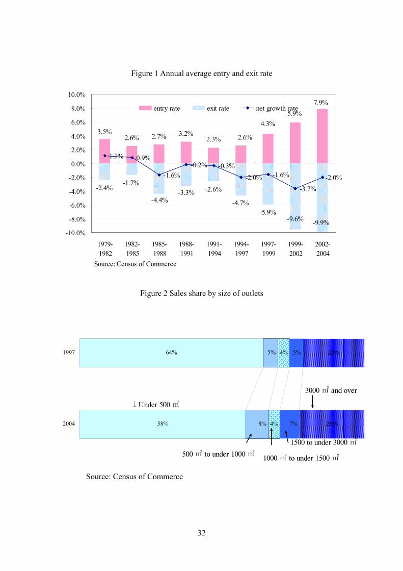
Figure 1 presents annual average entry and exit rates of retail outlets from 1979 to 2004. After 1994, the exit ratio has constantly exceeded the entry ratio and it increased in absolute value up to 9.9% in 2004. The entry rate began to increase since 1997 and amounted to 7.9% in 2004 probably reflecting the liberalization of entry restrictions.

= Figure 1 =

At the same time, sales share by size of outlets changed between 1997 and 2004 (Figure 2). Sales share for stores with floor space less than 500 m2 decreased from 64% to 58%. Conversely, sales share for stores with floor space 500 m2 or over, whose establishment was highly restricted under LSRS law, increased substantially. For example, stores with floor space 1500 m2 or over and under 3000 m2 increased from 5% to 70%. Stores with floor space of 3000 m2 or over also increased their share from 22% to 23%.

= Figure 2 =

Figure 3 presents changes in number of outlets by type and features of location between 1997 and 2004. On the whole, the number of large stores that have floor space more than 1000 m2 increased and their growth rate amounts to 3% on average. On the other hand, the growth rate of the number of small stores was –2% on average. Looking at the growth rate by type of location, in traditional cluster districts, such as the city center or station-side area, most of which are located in densely inhabited districts, both large stores and small stores decreased in number. Turning to the other districts, which are sometimes categorized as suburban area, there was marked growth, especially in large stores. For office districts and industrial districts, the growth rates of large stores exceeded more than 10%. This trend reflects the fact that densely inhabited districts had grown “thinner and broader” as a result of decreases of population in city centers and increases of population in suburban areas (METI 2006). This phenomenon is known as “hollowing out” of city center and some policy makers believe it has been accelerated by the increase of relocation of large stores from city center to suburban area. Recently, to revitalize city centers, some regional governments have introduced new regulations which restrict the new establishment of LSR with a floor space 10,000 m2 or over in suburban area. Our empirical assessment will provide some evidence on the causal

6

effect of LSR entry. In this study, reflecting the sharp contrast of outlet dynamics among areas and

districts, we classify (a) Near-station-type commercial district, (b) City-area-background-type commercial district, (c) Residential-background-type commercial district as the “city district” and the rest of the area as the “suburban district.”4

= Figure 3 = 4. Estimation Strategy

This paper examines causal effects of entry and exit of LSR on SME performance (e.g., sales, employment, and productivity) at the regional level. Let ENTRYit∈{0, 1} be an indicator of LRS entry in area i in period t. The average effect of treatment on the treated (ATT) is defined by

ATT =E (y1

it − y0it | ENTRYit = 1) = E (y1

it | ENTRYit = 1) − E (y0it | ENTRYit = 1),

where y1

it and y0it are the outcomes of SME in area i at period t with and without LSR

entry. As is well known, we cannot observe the last term; i.e., the SME performance in the area with LSR entry would not be obtained if there had been no entry. The estimates after replacing the last term with the observable E (y0

it | ENTRYit = 0) are consistent with the ATT only if the value inside the curly brackets in the following is equal to zero:

ATT = E (y1

it | ENTRYit = 1) − E (y0it | ENTRYit = 0)

+ {E (y0it | ENTRYit = 0) − E (y0

it | ENTRYit = 1)}. If not, the estimates suffer from so-called sample selection bias.

To avoid the sample selection bias, this paper adopts matching techniques; particularly, the propensity score matching method of Rosenbaum and Rubin (1983). Instrument variable method is an alternative technique, but it is always difficult to find convincing instruments. On the other hand, under some assumptions, the matching method enables us to estimate counterfactuals that cannot be directly observed. Furthermore, the matching method is a kind of non-parametric analysis and has the advantage that there is no need to specify the functional form of outcomes and

4 For a detailed definition of classification of location category, see Appendix Note 3-4-1, in METI (2006).

7

disturbances (Friedlander et al., 1997). Economic applications of matching methods have grown in recent years and they have been used for the evaluation of these: policy intervention in the labor market （Heckman et al., 1997; Blundell et al., 2002）, the effects of export or FDI on corporate performance (De Loecker, 2007; Navaretti and Castellani, 2004), and the effects of environmental regulation on plant birth ratio at the county level (List et al., 2003) etc.

The methodology proposed by Rosenbaum and Rubin (1983) is to find a vector of observable variables X which affect both the performance indicator y and the treatment variable ENTRY such that

{ } Xyy |ENTRY, 01 ⊥ , 1)|1(0 <=< XENTRYP ,

where ⊥ represents mathematical independence, and P( ∙ |X) denotes the predicted probability conditional on X, i.e., propensity score, of LSR entry. In other words, X is assumed to capture all the inherent differences in performance between the treated and control groups, i.e., regions with LSR entry and those without, respectively. This assumption is called conditional independence assumption (CIA). By using such a vector X, if regions have one LSR entry, the difference in performance of those areas purely represents the impact of LSR entry.

First, we estimate the propensity score of LSR entry at period t for area i as follows:

P (ENTRYit = 1) = F (Xit-1),

where Xit-1 is a vector of explanatory variables, such as population growth rate, number of LSR per population, and so forth. Let Pit be the predicted probability of LSR entry at period t for area i in the treatment group. Second, at each point in time and for each area i, a counterfactual area is selected as follows:

|Pit – Pjt| = min {Pit − Pkt}

k ∈ {l | ENTRYlt = 0}

We used one-to-one nearest neighbor matching technique. We imposed some assumptions required to assure consistency of the ATT estimates: y0

it ⊥ ENTRY it | Xit-1 and P (ENTRYit = 1| Xit-1) < 1. As suggested by Heckman et al. (1997), we assessed the impact of LSR entry by examining the change in the ex-post performance variables of the treatment and the control group from year t to year t+1. This indicator is called the

8

difference-in-difference (DID) estimator which is defined as the following indicator:

[ ]∑∈ ++ −−−=Ii tjtjtitiDID yyyy

n)()(1 0

,0

1,1,

11,α .

An alternative strategy is to compare directly the ex-post performance variables.

However, the DID estimator has advantages because it is independent from region-specific, unobservable, time-invariant factors which are not accounted for by X.

To ensure the validity of the estimation of propensity score and the matching based on the estimated propensity score, we statistically tested the condition of the balancing property as follows:

| ( 1| )ENTRY X P ENTRY X⊥ = ,

which means that, for a given propensity score, treatment observations are randomly chosen, and as a result, regions with LSR entry and regions without LSR entry are identical on average. To check whether the balancing property is satisfied, we implement the test of balancing property proposed by Becker and Ichino (2002). 5. Data

In this paper, we developed a new regional database by aggregating the individual data of the Wholesale and Retail Census (WR Census) performed by the Research and Statistics Department within the Minister’s Secretariat, Ministry of Economy, Trade and Industry (METI). This census covers all establishments active in the wholesale and retail sector. Since it was first performed in 1952, the survey has been conducted every 3 or 5 years. The latest data set is for 2004 and we used the data for 1997 and 2004. This covers the periods before and after the abolition of LSRS law. The WR Census contains establishment data on employment, sales, floor space, establishment age, and operating hours. We aggregated the data of individual stores at the regional level by sector and store size. Our sector classification consisted of the following: apparel retailing, food and beverage retailing, furniture retailing, appliances retailing, and generalized merchandise Stores (GMS).

The regional category comes from Minryoku statistical urban area, which is almost parallel to a metropolitan area in the US.5 Furthermore, as we discussed in 5 Minryoku urban area is basically defined according to commutation area. It consists of two regional categories. One is “economic area,” which is defined by dividing all Japan into 109 areas. The other is “urban area,” which consists of more than 1000 smaller areas. The concept of “urban area” is closer to commutation area. For details,

9

Figure 3, we divide each Minryoku statistical urban area into two groups; one is the “city district” and the other is the “suburban district” according to the location category in the WR census. Consequently, our observation units consisted of around 3,500 regional units. For our analysis, considering the difference in market characteristics, we classify our regional units in Tokyo, Nagoya, and Osaka metropolitan areas6 as “metropolitan area” and others as “provincial area.”

Our outcome variables are growth rate of sales, employment, wage payment, and productivity and entry and exit rate at the regional level. In our sample periods, the retail industry experienced a substantial increase in part-time worker ratio. Between 1997 and 2004, According to the Monthly Labor Survey (Ministry of Health and Labor), the part-time worker ratio for wholesale and retail industry has increased from 26.8% to 44.1%. And given the fact that there is substantial wage gap between full-time worker and part-time worker7, the differences of growth rate of employment and wage payment can be attributed to changes in the composition of type of employment. As for productivity index, since there is no information on capital stock at individual outlet-level, we calculated labor productivity index8.

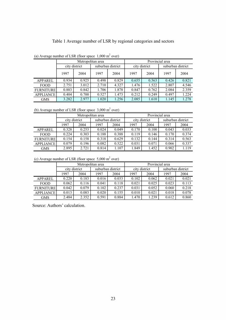
Table 1 presents the average number of LSR in each area by regional category and sector. We have three cut-offs for LSR according to floor space 1,000 m2 or over, 3,000 m2 or over, and 5,000 m2 or over, and they are shown in panels (a), (b), and (c), respectively. Two things are noteworthy about LSR with floor space 1,000 m2 or over. First, in suburban districts, the average number of LSR has been substantially increasing both in metropolitan areas and provincial areas. For example, in panel (a), while the average number of apparel retailing LSR in provincial areas/suburban districts has increased from 0.426 to 0.821. In contrast, the average number of LSR for provincial areas/city districts has slightly decreased from 0.655 to 0.563. This trend is the same as in Figure 3. Second, in most of the regional categories and industries, the number of LSR has either increased or remained constant; however, only the number of GMS in city districts has been decreasing both in metropolitan areas and provincial areas. For

see Asahi-Shimbunsha (2006). 6 Tokyo, Nagoya, and Osaka metropolitan areas are defined by Minryoku regional database (Asahi-Shimbunsha; 2006). It includes Tokyo, Nagoya, and Osaka and neighboring cities, such as Yokohama, Chiba, Saitama, Sakai, and Nara. 7 According to the Census of Wage Structure (Ministry of Health and Labor), while average hourly wage for full-time worker in Tokyo as of 2004 is 2774 yen, that for part-time worker is 1033 yen. 8 Adjustment of hours worked for labor input and data cleaning are explained in Appendix A.

10

example, in suburban districts, the average number of GMS in city district has increased from 1.020 to 1.256 and 1.145 to 1.278 for metropolitan and provincial areas, respectively. On the other hand, in city districts, the average number of GMS in suburban district has decreased from 3.282 to 2.977 and 2.085 to 1.610 for metropolitan and provincial areas, respectively. This fact might reflect recent stagnation of sales and profit for large department stores and supermarket chains in city districts.

== Table 1 ==

For our analysis, since we were interested in the effect of LSR entry on SME

performance at the regional level, we restricted our sample to those areas where there was no LSR in 1997. Moreover, we define LSR as those stores with floor space 1,000 m2 or over, whose entry was restricted under LSRS law as of 1997. SME is defined as those stores whose floor space is less than 1,000 m2 and operating under 14 hours.9 In addition, we excluded small stores that belong to the same building of LSR as tenants from our sample.10

Table 2 shows the sample size of our regional data and the ratio of areas with/without LSR entry to the total number of areas. As presented in Table 2, the ratio of areas with LSR entry in suburban districts is higher than that in city districts. Especially, in provincial areas/city district, the ratio of areas with LSR entry is quite small. For example, for food retailing stores, while the ratio of areas with LSR entry in provincial areas/suburban district is 63%, that in provincial areas/city district is 21%.

== Table 2 ==

Tables 3 compares SME performance between regions with/without LSR entry.

On the whole, SME performance in regions with LSR entry is better than those in regions without LSR entry. Especially, when LSR is defined as those stores with a floor space of 5,000 m2 or over, sharp contrasts have emerged. For example, scrutinizing the total effect in Table 3, panel (d), in provincial areas/suburban districts, the growth rate

9 In this period, small food retailing stores operating 24 hours for 7 days (convenience stores) have substantially increased market shares. To distinguish this innovative retail format from the traditional small retail outlet, SME are restricted to stores with less than 14 operating hours. For details of characteristics of convenience stores in Japan, see Larke (1994) and Mayer-Ohle (2003). 10 In WR census, we can identify those small stores that belong to the building of LSR with floor space 1,000 m2 or over.

11

of sales and employment for regions with LSR entry is 3.7% and 2.4% respectively, while that for regions without LSR entry is 2.1% and 1.5%. However, this result might reflect the fact that regions with LSR entry are attractive for enterprises in other industries and might have higher population growth rate and, as a result, have a positive effect both on LSR and SME. Thus, we should take care of these endogenous biases by the propensity score matching method. As for the growth rate of employment and wage payment, the former exceeds the latter in all regional categories. Especially, in provincial area/suburban districts, while the number of employment is increasing in area with LSR entry, the growth rate of wage payment is negative. It may suggest that increased competition accompanied with LSR entry has forced small retailers to replace full-time worker with part-time worker to save cost.

== Table 3 ==

6. Empirical Results

We started by running a probit regression to derive the probability of LSR entry with the regional data. As we mentioned in the explanation of Table 2, our analytical sample is restricted to those areas where there were no LSR in 1997. We define an entry dummy as 1 if LSR has entered the area between 1997 and 2004, and 0 otherwise. The propensity of LSR entry is considered to be a function of the number of LSR per population (large_pop), its square (large_pop2), the number of LSR in surrounding regions (largen3_pop), population growth rate (population growth), log of population (log_population), income inequality index (income), and the ratio of daytime population to nighttime population (day-by-night).11 Detailed definitions and summary statistics are presented in Table 4 and Table 5, respectively. All independent variables except population growth are values in 1997.

== Table 4 == == Table 5 ==

The estimation result for the probit model is presented in Table 6. We found the

number of LSR per population, its squares, and the size of population have significant

11 In addition to variables explained above, we tried to include car ownership ratio, the ratio of people aged 65 or over to total population and income inequality index by area. However, their coefficients are not significant, and when including these variables the test of balancing property is not satisfied. Therefore, we dropped these variables.

12

coefficients. Using this result of probit estimation, we retrieved the propensity score to match areas with LSR entry (treated group) to those without LSR entry that are similar in terms of their observable characteristics (control group). Areas are matched separately for each regional category and industry using one-to-one matching with replacement. The common support assumption is also imposed as suggested in literature. As we discussed in section 4, in order to verify whether the balancing properties are satisfied or not, as suggested by Becker and Ichino (2002), we perform the following algorithm: (i) splitting the sample such that average propensity scores of the treated and control groups do not differ, and (ii) within each interval, testing whether the means of every element of covariate X are different between treated and control groups (balancing hypothesis). If there are no statistically significant differences between the two, then we moved forward to compare the treatment group and control group.

== Table 6 ==

Our outcome variables included the balancing hypothesis of SME annual growth rate of sales, number of employees, wage payment and productivity, and entry and exit rate for SME at the regional level. In addition, to highlight the effect on incumbent continuing stores (Existing SME), we calculated growth rate of sales and employment for those SME which were observed both in 1997 and 2004 in our panel data set. Table 7 (a) presents the comparison between areas with LSR entry (treated) and matched areas without LSR entry (control) by region. There are two noteworthy findings. First, entry rates are significantly different between treated and control except for provincial areas/city districts, suggesting that LSR entry promoted new entry. Second, for growth rate of sales and employment, we did not find any significant effect. For those stores that continued functioning, there is no significant effect.

One may be interested in the impact of LSR entry by the floor size. As we present Table 3, the differences of SME performance become more significant as the size of LSR becomes larger. Therefore, in panel (b) and (c) in Table 7, we restrict our treatment group to areas with LSR whose floor space are 3,000 m2 or over and 5,000 m2 or over, respectively. As for the result of LSR with floor space 3,000m2 or over, significant positive effect on almost all performance indicator has emerged in provincial area/city districts. However, in other regional categories, any significant effect cannot be found except for a few exception. The effects of LSR entry become clearer when we restrict treatment group to those stores with floor space 5,000 m2 or over. In provincial area, we found additional significant positive effect on productivity in city districts. And in

13

suburban area, there is positive effect on existing SME's productivity.

== Table 7 ==

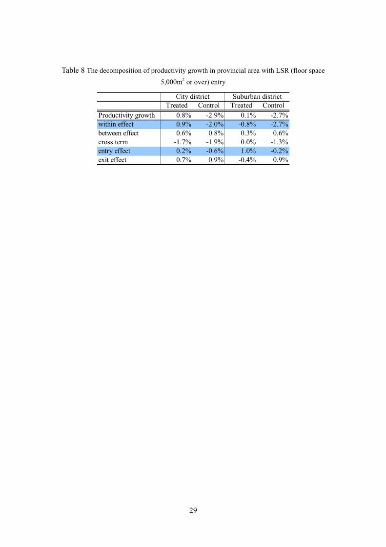
What is the key driver of SME's productivity growth? Following from Foster et al. (2008), we decompose the total labor productivity growth rate into the 5 factors; (1) a within effect, (2) a between effect, (3) a covariance term, (4) an entry effect and (5) an exit effect12. While a within effect is weighted average of individual outlet-level productivity growth, a between effect and the entry and exit effects are the contribution by changes in share of continuing, entering and exiting outlets, respectively. The decomposition of productivity growth in provincial area/city and suburban districts for panel (c) of Table 7 are presented in Table8. In both districts, within effect and entry effect for treatment group are higher than those of control groups. It implies that in provincial area, LSR entry may have some spillover effects on existing and entering SMEs.

== Table 8 == However, on the whole, the effect of LSR entry is quite limited. There is almost

no significant effect on sales and employment in metropolitan areas/suburban districts. The growth rate or sales and employment for existing SME do not have significant difference between treatment group and control group except for provincial areas/city districts. 7. Conclusion

In this paper, we quantified the effect of liberalization of entry restriction for large stores on SME performance for the Japanese retailing sector in the late 1990s. While previous studies restrict their focus of study to the effect on SME employment, our newly created regional database enables us to control detailed regional characteristics and shed light on various performance indicators, such as sales, wage payment and productivity. To tackle the endogeneity between LSR entry and SME performance, we used the propensity score matching method. Comparison with matched sample suggested that LSR entry did not have any negative effect on SME performance. Instead, we found a positive effect on the SME's sales and employment in some cases, which coincide with the findings in European studies such as those by Bertrand and Kramarz

12 For detailed definition of productivity decomposition by Foster et al. (2008), see Appendix B.

14

(2002), and Schivarrdi and Viviano (2007). The positive effects of LSR entry are found in provincial area/suburban district when we focus on the effect of entry of LSR with floor space 5000m2 or over. And we found LSR entry has positive effect not only on employment but also sales, wage payment and productivity.

In Japan, in order to prevent “hollowing out” of city center district, a variety of measures to revitalize those districts are currently being studied, and some regional governments have introduced a new restriction for an establishment of new large stores with floor spaces 10,000 m2 or over in suburban districts. However, our results imply such a policy may not bring about any gain for SME in city center and hinder job creation in suburban districts.

In terms of future work, we would like to corroborate our results by dividing our sample in various dimensions. Since the impact of LSR entry might differ according to region, by dividing our regional category in further detail, we expect to gain further evidence and policy implications concerning the effects of LSR entry.

15

Appendix A: Procedure to estimate outlet-level productivity

index

A1. The Definition of productivity growth

This appendix explains how we construct productivity index at outlet-level. Since there is no information on capital stock in WR census, the productivity index we used is the labor productivity index, which is defined as follows;

ititit LQP lnln −= , (2.1)

where Q is real gross output and L is labor input. We used gross margin as output. Since margin ratio in WR census is available only at the firm level, not at the establishment level, we estimated gross margin following from the estimation method by U.S Bureau of Economic Analysis (hereafter BEA). In BEA approach, the constant value of gross margin, R, in industry i and year t is defined as follows;

Rit = ri

base*Qit,

where ri

base is the nominal value of margin ratio, in detailed sectral level in base year and Q is deflated sales value. We calculated base year margin ratio with 2002 Wholesale Retail Census in 4-digit sector level. As for the deflator for retailing sales, we calculated retailing price index by year, prefecture, and commodity with using “Consumer Price Index” (Ministry of Internal Affaires and Communications) and “Retail Price Survey” (Ministry of Internal Affaires and Communications).

A2. Adjustment hours worked

As for labor input, since some retailers make extensive use of part-time labor, it is essential to incorporate the differentials in composition of labor input among outlets. Besides, it is well known that there is a significant hourly wage gap between full-time workers and part-time workers. Therefore, it would be better to take into account not only differentials in hours worked but also those in wage rate. However, data constraints make it difficult to construct FTE labor inputs. While the data for 2004 contained the proportion of part-time workers, data for 1997 provided only the total number of

16

workers. Average hours worked and hourly wage were not available at the establishment level.

We estimated the hours worked and hourly wage using the following methodology: for hours worked by part-time workers, since the 2002 data provides both actual numbers of part-time workers and FTE number of part-time workers, we assumed that average hours worked by part-time workers by retail format categories were constant between 1997 and 2004, and constructed hours worked ratio by retail format categories. As average hourly wage for both full-time workers and part-time workers are available from the Census of Wage Structure (Ministry of Health, Labor and Welfare) every year by prefecture, we calculated the hourly wage ratio by prefecture. For the number of part-time workers in 1997, we adjusted the 1997 data by linking with the Establishment and Enterprise Census (Ministry of Internal Affairs and Communications), which provides proportions of part-time workers at the establishment level. Our labor input indicator is defined as follows:

Labor input = # of full-time workers

+ # of part-time workers × hours worked ratio × wage ratio

A3. Productivity and Establishment Age

In our analysis, we deleted those establishments whose age is less than 2 years. This is because their productivity level cannot be estimated correctly and as a result, there is serious bias in the relationship between productivity and age of establishment as depicted figure A1. The reason for surprisingly low productivity of young establishment is that there is inconsistency between young outlets and old outlets in terms of unit of survey period. For young outlets, although the length of operation might be less than 12 months, all outlets are requested to report “annual sales.” On the other hand, input value is measured by employment at the point of survey. Therefore, output value for young outlets might be underestimation. If more detailed information of market entry, e.g. date or month of entry as well as year of entry, is available, output value for young outlets can be adjusted. However, since there is only year of entry in the questionnaire of WR census, we dropped young outlets from our sample.

= Figure A1 =

17

Appendix B: The decomposition of productivity growth

Productivity decomposition is a method for linking aggregate productivity growth to micro productivity growth. Aggregate productivity growth is the weighted average of establishment-level productivity growth, where the weights are related to the importance of the establishment in the industry:

∑= ititt PsP (B1)

where tP is the index of industry productivity, its the employment share of

establishment i in industry13, and itP an index of establishment-level productivity. Foster et al. (2001) review the computations used in empirical studies that decompose aggregate productivity growth into components related to within-establishment productivity growth, reallocation, and the effects of exit and entry. Their decomposition is:

∑∑∑∑∑

∈ −−−∈ −

∈∈ −−∈ −

−−−+

ΔΔ+Δ−+Δ=Δ

Xi tititNi titit

Ci ititCi ittitCi ititt

PPsPPs

sPsPPPsP

)()(

)(

1111

111

(B2)

where C denotes continuing establishments, N denotes entering establishments, and X denotes exiting establishments. In the decomposition, aggregate productivity growth between the two periods is composed of five components. The five components distinguished are (1) a within-establishment effect – within-establishment growth weighted by initial output shares; (2) a between-establishment effect – changing output shares weighted by the deviation of initial establishment-level productivity and initial industry-level productivity; (3) a covariance term – the sum of establishment-level productivity growth multiplied by establishment share change; (4) an entry effect –a year-end share-weighted sum of the difference between the productivity of entering establishments and initial industry productivity; and (5) an exit effect – an initial share-weighted sum of the difference between initial productivity of exiting establishments and initial industry productivity. The between-establishment and the entry and exit terms involve a deviation of establishment-level productivity from initial

13 For example, Foster et al (2008) argues since sales figure sometimes highly fluctuates, they used labor input as share weight.

18

industry-level productivity. A continuously operating establishment with increasing shares makes a positive contribution to aggregate productivity only if it initially has the industry average. Entering (exiting) establishments contribute positively only if they have lower (higher) productivity than the initial average. We apply the decomposition in equation (B2) by industry and region. Based on previous studies, we use the labor input for share weights14. We use the nominal output weights to average across sales formats. An average productivity growth and its decomposition are presented in Table B1. Besides, this table compares the pattern of US productivity dynamics estimated by Foster et al (2008). Although sample period is substantially different, the magnitude and the pattern of productivity growth are quite similar between US and Japan. For example, both US and Japan have achieved around 1.1%-1.4% productivity growth annually from 1987 to 1997 for US and from 1997 to 2004 for Japan. Besides, the contribution of reallocation is quite high for both US and Japan. It accounts for 74% (1.06%/1.43%) and 84% (0.96%/1.14%) of total productivity growth rate for US and Japan, respectively. One thing we should note is that while entry share effects exceeds exit share effect in US; the latter is large than the former in Japan. This point might reflect Japans’ negative growth for number of outlets.

== Table B1 ==

Table B2 presents productivity dynamics and contribution of LSR by industry. Three finds stand out form this table. First, looking at a contribution of large-scale outlet, one for entry share effect is significantly high. For sector total, it explains 60% (6.3%/9.8%) of overall entry share effect. In case of Generalized Merchandise Store (GMS), Furniture and Appliances, in contrast to negative or zero contribution by SMEs, that of LSR entry is quite high. Second, except for GMS, the contributions of small outlet for exit share effect are substantially large. Since the contribution of large-scale outlet for exit share effect is sometime negative, that of small outlet accounts for most of exit share effect. Third, the contributions of SMEs for between share effects are consistently positive and account for most of between share effects except for GMS. These facts suggest there is sorting effect of LSR entry on SMEs’ performance. LSR entry might promote competition among retailers and it induces unproductive small stores to drive out from markets. It might be reflected by the positive exit share effect of SMEs. At the same time, positive between share effects by SMEs implies that newly opened LSR

14 For example, Foster et al (2008) argues since sales figure sometimes highly fluctuates, they used labor input as share weight.

19

attracts consumers in broader retail trading area, and it might bring a spillover effect on SMEs with higher productivity level.

== Table B2 ==

20

References Abe, N., and D. Kawaguchi, 2008, “Incumbent’s Price Response to New Entry:

Japanese Supermarket Case,” mimeograph.

Asahi-Shimbunsha, 2006, Minryoku, The Asahi Shimbun Company, Tokyo.

Baily, M., 1993, “Competition, Regulation, and Efficiency in Service Industries,” Brooking Papers: Microeconomics, Vol.2, pp.71-130.

Basker, E., 2005, “Job Creation or Destruction? Labor-Market Effects of Wal-Mart Expansion,” Review of Economics and Statistics, Vol.87, No.1, pp.174-183.

Basker, E., 2007, “The Causes and Consequence of Wal-Mart’s Growth,” Journal of Economic Perspective, Vol.21, No.3, pp.177-198.

Becker, S. O., and A. Ichino., 2002, “Estimation of Average Treatment Effects Based on Propensity Scores,” The Stata Journal, Vol. 2, No.4, pp.358-377.

Bertrand, M., and F., Kramarz, 2002, “Does Regulation Hinder Job Creation? Evidence from the French Retail Industry,” Quarterly Journal of Economics, Vol.117, No.4, pp.1369-1413.

Blundell R., M., Costa Dias, 2002, “Alternative Approached to Evaluation in Empirical Microeconomics,” Cemmap Working Paper CWP 10/02.

De Loecker J., 2007, “Do Exporters Generate Higher Productivity? Evidence from Slovenia,” Journal of International Economics, Vol.73, pp.69-98.

Flath, D., 1990, “Why are There so Many Retail Stores in Japan?” Japan and the World Economy, Vol.2, pp.365-386.

Friedlander, D., D., Greenberg, and P., Robins, 1997, “Evaluating Government Training Programs for the Economically Disadvantaged,” Journal of Economic Literature Vol.35, pp.1809-1855.

Foster, L., J., Haltiwanger and C.J. Krizan, 2001, "Aggregate Productivity Growth: Lessons from Microeconomic Evidence," Edward, D., M., Harper and C., Hulten eds., New Directions in Productivity Analysis, University of Chicago Press.

Foster, L., J., Haltiwanger and C.J. Krizan, 2008, "Market Selection, Reallocation, and Restructring in the U.S. Retail Trade Sector in the 1990s,” Review of Economics and Statistics, Vol. 88, No.4, pp.748-758.

21

Heckman J., H., Ichimura, P., Todd, 1997, “Matching as an Econometric Evaluation Estimator: Evidence Evaluating a Job Training Program,” Review of Economic Studies, Vol.64, pp.605-654.

Igami, M., 2007, “Does Big Drive Out Small?: Entry and Differentiation in the Tokyo Food Supermarkets after Deregulation,” mimeograph.

Larke, R., 1994, Japanese Retailing, London: Routledge.

List, J., D., Millimet, P., Fredriksson, and W., McHone, 2003, “The Effects of Environmental Regulations on Manufacturing Plant Births; Evidence From A Propensity Score Matching Estimator,” Review of Economics and Statistics, Vol.85, No.4, pp.944-952.

METI (Ministry of Economy, Trade and Industry), 2006, “White Paper on Small and Medium sized Enterprises 2006,” Available from the web site: http://www.chusho.meti.go.jp/pamflet/hakusyo/h18/download/2006hakusho_eng.pdf

Mayer-Ohle, H., 2003, Innovation and Dynamics in Japanese Retailing - From Techniques to Formats to Systems, Hampshire: Palgrave Macmillan.

Mckinsey Global Institute, 1994, “Employment Performance,” MGI research report, November 1994.

Mckinsey Global Institute, 1997, “Removing Barriers to Growth and Employment in France and Germany,” MGI research report, March 1997.

Mckinsey Global Institute, 2000, “Why the Japanese Economy is not Growing; Micro Barriers to Productivity Growth,” MGI research report, July 2000.

Navaretti, G B., and D. Castellani, 2004, “Investments Abroad and Performance at Home: Evidence from Italian Multinationals,” CEPR Discussion Paper, No.4284.

Neumark, D., J., Zhang, and S., Stephen, 2008, “The Effects of Wal-Mart on Local Labor Market,” Journal of Urban Economics, Vol.63, No.2, pp.405-430.

Nishida, M., 2008, "Estimating a Model of Strategic Network Choice: the Convenience-Store Industry in Okinawa,", NET Institute Working Paper No. 08-27.

22

Nishimura, G., K., T., Tachibana, 1996, “Entry Regulations, Tax Distortions and the Bipolarized Market: the Japanese Retail Sector,” Sato, R., R. Ramachandran., H., Hori eds. in Organization, Performance, and Equity: Perspectives on the Japanese Economy, Boston; Kluwer Academic Publication, pp.1-57.

Olley, S., and A., Pakes, 1996, “The Dynamics of Productivity in the Telecommunications Equipment Industry,” Econometrica, Vol.6, No.6, pp.1263-1297.

Pavcnick, N., 2002, “Trade Liberalization, Exit and Productivity Improvement: Evidence from Chile Plant,” Review of Economic Studies, Vol.69, No.1, pp.245-276.

Rosenbaum, P., and D., Rubin, 1983, The Central Role of the Propensity Score in Observational Studies for Causal Effects, Biometrika Vol.70, pp.41-55.

Schivarrdi, F., and E.,Viviano, 2007, “Entry Barriers in Italian Retail Trade,” Bank of Italy Economic Research Paper, No.616.

23

Table 1 Average number of LSR by regional categories and sectors

(a) Average number of LSR (floor space 1,000 m2 over)

1997 2004 1997 2004 1997 2004 1997 2004

APPAREL 0.934 0.925 0.498 0.829 0.655 0.563 0.426 0.821FOOD 2.751 3.012 2.710 4.327 1.476 1.522 2.807 4.546

FURNITURE 0.883 0.842 1.706 1.878 0.847 0.762 2.084 2.359APPLIANCE 0.404 0.700 0.527 1.473 0.212 0.249 0.497 1.224

GMS 3.282 2.977 1.020 1.256 2.085 1.610 1.145 1.278

(b) Average number of LSR (floor space 3,000 m2 over)

1997 2004 1997 2004 1997 2004 1997 2004APPAREL 0.328 0.253 0.024 0.049 0.170 0.100 0.043 0.033

FOOD 0.224 0.303 0.188 0.388 0.119 0.146 0.170 0.374FURNITURE 0.154 0.158 0.318 0.629 0.132 0.144 0.314 0.563APPLIANCE 0.079 0.196 0.082 0.522 0.031 0.071 0.066 0.337

GMS 2.895 2.721 0.814 1.107 1.849 1.452 0.902 1.119

(c) Average number of LSR (floor space 5,000 m2 over)

1997 2004 1997 2004 1997 2004 1997 2004APPAREL 0.220 0.183 0.016 0.033 0.102 0.062 0.021 0.021

FOOD 0.062 0.116 0.041 0.118 0.021 0.025 0.023 0.113FURNITURE 0.042 0.079 0.102 0.237 0.031 0.052 0.060 0.218APPLIANCE 0.013 0.083 0.020 0.155 0.010 0.021 0.018 0.078

GMS 2.484 2.352 0.591 0.884 1.470 1.239 0.612 0.860

Metropolitan area Provincial areacity district suburban district

Metropolitan area Provincial areacity district suburban district city district suburban district

Provincial areacity district suburban district city district suburban district

Metropolitan area

city district suburban district

Source: Authors’ calculation.

24

Table 2 The number and ratio between areas with/without LSR entry

citydistrict

suburbandistrict

citydistrict

suburbandistrict

145 167 300 358 970% of LSR entered areas 9% 18% 10% 28% 18%

% of no LSR areas 91% 82% 90% 72% 82%56 56 206 131 449

% of LSR entered areas 20% 54% 21% 63% 37%% of no LSR areas 80% 46% 79% 37% 63%

132 79 260 145 616% of LSR entered areas 15% 16% 7% 22% 13%

% of no LSR areas 85% 84% 93% 78% 87%188 166 408 340 1102

% of LSR entered areas 19% 45% 7% 31% 22%% of no LSR areas 81% 55% 93% 69% 78%

11 83 68 163 325% of LSR entered areas 9% 27% 12% 25% 22%

% of no LSR areas 91% 73% 88% 75% 78%Note: 1) LSR is defined as those store with floor space 1,000m2 or over.2)"LSR entered areas" are the areas where there was no LSR in 1997, but there were some LSR in 2004.3)"no LSR areas" are the areas where there was no LSR in both 1997 and 2004.

total

GMS

APPLIANCE

FURNITURE

FOOD

APPAREL

# of ares where there wasno LSR in 1997.

Total

Provincial areaMetropolitan area

Total

Sector

Total

Total

Total

25

Table 3 Simple comparison of average SME's performance by area with or without LSR entry at regional-level

Simple comparison of average SME's performance by area with or without LSR entry at regional-levela) Major Urban Area - city district

w/o LSR entry w/ LSR (1000m2or over) entry

w/ LSR (3000m2or over) entry

w/ LSR (5000m2or over) entry

Sales change -1.7% -2.2% -3.8% -2.1%Employment change -0.5% 0.1% 0.0% 3.2%Wage payment -2.2% -1.2% -1.4% 1.5%Entry rate 16.9% 20.1% 23.9% 27.1%Exit rate 29.5% 26.7% 24.3% 21.5%Productivity change -4.2% -3.0% -5.1% -5.1%

b) Major Urban Area - suburban district

w/o LSR entry w/ LSR (1000m2or over) entry

w/ LSR (3000m2or over) entry

w/ LSR (5000m2or over) entry

Sales change 22.9% 0.8% -1.2% 0.2%Employment change 9.0% 2.5% 1.5% 4.2%Wage payment 5.7% -0.1% -0.6% 0.9%Entry rate 24.7% 25.6% 25.4% 28.0%Exit rate 28.7% 27.2% 26.3% 25.0%Productivity change -1.7% -2.6% -2.5% -0.9%

c) Provincial area - city district

w/o LSR entry w/ LSR (1000m2or over) entry

w/ LSR (3000m2or over) entry

w/ LSR (5000m2or over) entry

Sales change -4.2% -5.1% -3.1% -1.8%Employment change -2.5% -2.9% -2.9% -2.6%Wage payment -3.5% -4.0% -4.3% -4.2%Entry rate 12.3% 13.8% 10.7% 7.1%Exit rate 30.7% 29.3% 28.2% 25.6%Productivity change -3.7% -3.6% -0.9% 0.8%

d) Provincial area - suburban district

w/o LSR entry w/ LSR (1000m2or over) entry

w/ LSR (3000m2or over) entry

w/ LSR (5000m2or over) entry

Sales change 2.1% 3.7% 20.6% 35.6%Employment change 1.5% 2.4% 10.0% 15.3%Wage payment -0.3% -0.3% 4.0% 6.6%Entry rate 20.0% 21.8% 23.5% 24.5%Exit rate 26.5% 26.1% 22.9% 20.5%Productivity change -2.8% -1.8% -0.6% 1.5% Note: All performance indicators are annual average growth rate of outcome variables between 1997 and 2004.

26

Table 4 Definition of Variables in probit model Variable name Explanation/Definition Date Sourcelarge_entry1,000 [LSR with more than 1,000m2 floor entered area] dummy 1997, 2004 Authors calculationlarge_pop # of LSR per 1,000 persons 1997, 2004 Minryokularge_pop2 squares of # of LSR per 1,000 persons 1997, 2004 Minryokulargen3_pop # of LSR per 1,000 persons within neaby regions except own region 1997, 2004 Minryokupopulation growth population growth rate from the previous year (%) in the same region 1996-1997, 2003-2004 Minryokulog(population density) logged population density 1997, 2004 Minryokulog(population) logged population 1997, 2004 Minryokuincome income inequality (national average=100) 1997, 2004 Minryokudaybynight ratio of daytime population to night time population 1996 Minryoku

27

Table 5 Summary Statistics variables N mean sd p25 p75large_entry1000 3462 0.213 0.410 0.000 0.000large_pop 3462 0.009 0.021 0.000 0.011large_pop2 3462 0.001 0.004 0.000 0.000largen3_pop 3462 0.013 0.014 0.004 0.017population growth rate 3462 -0.005 0.049 -0.037 0.026ln(population density) 3462 6.186 1.605 5.044 7.257log(population) 3462 11.493 0.858 10.885 11.989income 3462 0.923 0.222 0.769 1.044day-by-night 3462 1.002 0.861 0.897 1.002

Table 6 Estimation results for the probit model

Dependent Variable

Coef. s.e. z-ratio p-valuelarge_pop 9.749 2.037 4.79 0.00large_pop2 -13.167 10.690 -1.23 0.22largen3_pop 0.228 2.187 0.1 0.92population growth rate 1.012 0.722 1.4 0.16ln(population density) 0.034 0.027 1.25 0.21log(population) 0.108 0.035 3.08 0.00income -0.263 0.217 -1.21 0.23day-by-night 0.047 0.029 1.61 0.106Constant -2.014 0.410 -4.92 0.00Region Dummy YesIndustry Dummy YesN 3462Pseudo R2 0.1041Log likelihood -1608.192

Dummy variable for LSR (floor>=1,000)entered area

28

Table 7 Comparison with matched sample by region and district (a) The effects of LSR (with more than 1,000 m2 floor space) entry on SME

Treated Control t Treated Control t Treated Control t Treated Control t sales change -0.022 -0.037 1.03 0.006 0.010 -0.26 -0.052 -0.046 -1.12 0.022 -0.004 0.94employment change 0.000 -0.009 0.77 0.024 0.018 0.62 -0.029 -0.030 0.30 0.018 0.004 1.47wage payment -0.013 -0.023 0.85 -0.001 0.000 -0.16 -0.040 -0.043 0.68 -0.005 -0.010 0.76entry rate 0.200 0.155 2.42 ** 0.256 0.236 1.31 0.137 0.105 3.10 *** 0.219 0.198 2.25 **exit rate 0.266 0.286 -1.13 0.273 0.279 -0.49 0.293 0.311 -1.17 0.257 0.274 -1.61productivity change -0.030 -0.052 2.11 ** -0.028 -0.021 -0.84 -0.037 -0.029 -1.21 -0.022 -0.027 1.10sales change -0.044 -0.038 -0.90 -0.036 -0.033 -0.55 -0.043 -0.039 -1.26 -0.029 -0.038 1.71 *employment change -0.013 -0.006 -1.89 * -0.004 -0.004 -0.15 -0.012 -0.009 -1.13 -0.005 -0.005 -0.13wage payment -0.019 -0.017 -0.77 -0.017 -0.012 -1.47 -0.021 -0.021 -0.03 -0.016 -0.013 -1.40productivity change -0.608 -0.289 -0.96 -0.512 -0.331 -0.84 -0.796 -0.324 -1.36 -0.332 -0.389 0.72

(b) The effects of LSR (with more than 3,000 m2 floor space) entry on SME

Treated Control t Treated Control t Treated Control t Treated Control t sales change -0.038 -0.037 -0.04 -0.016 0.010 -1.29 -0.031 -0.046 1.13 0.140 -0.004 2.56 **employment change 0.000 -0.009 0.60 0.012 0.018 -0.58 -0.029 -0.030 0.19 0.071 0.004 3.64 ***wage payment -0.014 -0.023 0.61 -0.006 0.000 -0.69 -0.043 -0.043 -0.10 0.030 -0.010 3.39 ***entry rate 0.239 0.155 3.07 *** 0.250 0.236 0.62 0.107 0.105 0.12 0.232 0.198 1.97 **exit rate 0.243 0.286 -1.50 0.263 0.279 -0.74 0.282 0.311 -0.91 0.219 0.274 -2.69 ***productivity change -0.051 -0.052 0.05 -0.027 -0.021 -0.55 -0.009 -0.029 1.71 * -0.016 -0.027 1.26sales change -0.045 -0.038 -0.66 -0.030 -0.033 0.56 -0.033 -0.039 0.98 -0.008 -0.038 2.93 ***employment change -0.009 -0.006 -0.52 -0.003 -0.004 0.03 -0.016 -0.009 -1.56 -0.003 -0.005 0.49wage payment -0.021 -0.017 -0.79 -0.015 -0.012 -0.58 -0.028 -0.021 -1.48 -0.014 -0.013 -0.12productivity change -0.486 -0.289 -0.32 -0.442 -0.331 -0.47 -0.233 -0.324 0.67 -0.256 -0.389 0.94

(c) The effects of LSR (with more than 5,000 m2 floor space) entry on SME

Treated Control t Treated Control t Treated Control t Treated Control t sales change -0.021 -0.037 0.52 -0.004 0.010 -0.52 -0.018 -0.046 1.61 0.248 -0.004 3.48 ***employment change 0.032 -0.009 1.52 0.037 0.018 1.20 -0.026 -0.030 0.44 0.106 0.004 4.38 ***wage payment 0.015 -0.023 1.55 0.009 0.000 0.72 -0.042 -0.043 0.04 0.047 -0.010 3.94 ***entry rate 0.271 0.155 2.76 *** 0.272 0.236 1.18 0.071 0.105 -1.33 0.238 0.198 1.87 *exit rate 0.215 0.286 -1.57 0.250 0.279 -0.99 0.256 0.311 -1.26 0.190 0.274 -3.21 ***productivity change -0.051 -0.052 0.03 -0.014 -0.021 0.47 0.008 -0.029 2.38 ** 0.001 -0.027 2.70 ***sales change -0.051 -0.038 -0.73 -0.025 -0.033 0.90 -0.025 -0.039 1.64 0.017 -0.038 4.06 ***employment change -0.005 -0.006 0.07 -0.001 -0.004 0.43 -0.015 -0.009 -0.98 0.000 -0.005 1.06wage payment -0.012 -0.017 0.52 -0.015 -0.012 -0.38 -0.027 -0.021 -0.99 -0.012 -0.013 0.37productivity change -1.147 -0.289 -0.84 -0.514 -0.331 -0.55 -0.217 -0.324 0.58 -0.026 -0.389 2.10 **

Note:"***","**","*"denote significance at 1%, 5% and 10%, respectively.

ExistingSME

Major Urban Area - suburban district Provincial area - suburban districtProvincial area - city districtMajor Urban Area - city district

all SME

Provincial area - suburban districtProvincial area - city districtMajor Urban Area - city district

Major Urban Area - suburban district Provincial area - suburban districtProvincial area - city district

ExistingSME

Major Urban Area - suburban district

Major Urban Area - city district

all SME

ExistingSME

all SME

29

Table 8 The decomposition of productivity growth in provincial area with LSR (floor space 5,000m2 or over) entry

Treated Control Treated ControlProductivity growth 0.8% -2.9% 0.1% -2.7%within effect 0.9% -2.0% -0.8% -2.7%between effect 0.6% 0.8% 0.3% 0.6%cross term -1.7% -1.9% 0.0% -1.3%entry effect 0.2% -0.6% 1.0% -0.2%exit effect 0.7% 0.9% -0.4% 0.9%

City district Suburban district

30

Table B1 International comparison on labor productivity growth between US and Japan

Periodentry share exit share

Japan 1997-2004 1.43% 0.39% 1.06% 0.87% -1.89% 2.07% 0.64% 1.43%USA 1987-1997 1.14% 0.18% 0.96% 0.27% -0.45% 1.13% 0.62% 0.51%

Source: For Japan, authors' calculation. Unit: annual average growth rate.For USA, table 3 in Foster, Haltiwanger and Krizan (2006)

productivitygrowth

withineffect

Reallocation effectbetween

share cross share Net entry

31

Table B2 Decomposition of labor productivity growth for 1997-2004 and contribution of Lager outlets

Large outlet 0.93% 0.33% 0.13% -0.30% 0.89% -0.19%small outlet -0.10% -0.41% 0.74% -1.57% 0.40% 0.81%

Large outlet 0.04% 0.07% -0.07% -0.11% 0.43% -0.23%

small outlet -1.10% -1.69% 0.59% -1.33% 0.36% 0.91%

Large outlet 0.74% 0.19% 0.10% -0.23% 0.70% -0.14%small outlet 0.81% 0.27% 0.96% -2.09% 0.90% 0.89%

Large outlet 0.27% 0.11% -0.13% -0.29% 1.23% -0.61%small outlet -2.36% -1.76% 0.46% -1.09% -1.37% 1.33%

Large outlet 2.47% 0.09% -0.16% -0.07% 2.60% -0.43%small outlet -3.03% -1.84% 0.61% -0.69% -1.11% 0.44%

Large outlet 2.84% 2.07% 1.07% -1.34% 1.13% 0.11%small outlet 0.37% 0.01% 0.09% -0.03% 0.00% 0.10%

Small outlets are those outlets whose floor space is less than 1000m2.

0.69%-1.06% -1.63% 0.51% 0.79%

-0.74%

-2.31%

1.49%

-1.37%

-1.76% 0.46%

-1.43%

1.56% 0.46% 1.06%

-0.56%

-2.10% -1.63% 0.34%

0.83% -0.07% 0.87% -1.87%

3.21% 2.10% 1.16% -1.37%

0.00%

1.60% 0.76%

INDUSTRY

GMS 1.13% 0.21%

1.29% 0.63%

-0.14% 0.71%

ALL

FOOD

FURNITURE

APPLIANCE

APPAREL

productivitygrowth within share between

share exit share

share of productivity growth

cross share entry share

32

Figure 1 Annual average entry and exit rate

3.5%2.6% 2.7% 3.2%

2.3% 2.6%

4.3%5.9%

7.9%

-2.4%-1.7%

-4.4%-3.3% -2.6%

-4.7%-5.9%

-9.6% -9.9%

1.1% 0.9%

-1.6%-0.2% -0.3%

-2.0% -1.6%

-3.7%-2.0%

-10.0%

-8.0%

-6.0%

-4.0%

-2.0%

0.0%

2.0%

4.0%

6.0%

8.0%

10.0%

1979-1982

1982-1985

1985-1988

1988-1991

1991-1994

1994-1997

1997-1999

1999-2002

2002-2004

entry rate exit rate net growth rate

Source: Census of Commerce

Figure 2 Sales share by size of outlets

64%

58%

5%

8%

4%

4%

5%

7%

22%

23%

1997

2004

↓Under 500 ㎡

500 ㎡ to under 1000 ㎡ 1000 ㎡ to under 1500 ㎡

1500 to under 3000 ㎡

3000 ㎡ and over

Source: Census of Commerce

33

Figure 3 Changes in number of outlets by type and features of location between 1997 and 2004

-2%

-3%

-3%

0%

-3%

6%

-1%

0%

-1%

3%

-1%

-3%

-1%

6%

1%

14%

6%

13%

9%

-5%

-5% -3% -1% 1% 3% 5% 7% 9% 11% 13% 15%

Near-station-type

City area-background type

Residential-background-type

Roadside-type

Other commercialclusters

Office district

Residential district

Industrial district

Other district

TO

TA

LC

om

merc

ial d

istirc

t Small stores

Large stores

Unit: Annual average growth rate (%)

City distr ict

Suburban distr ict

Source: Census of Commerce

34

Figure A1 Productivity shift since market entry

-3.5

-3

-2.5

-2

-1.5

-1

-0.5

0

0.5

1

lessthan 1year

1～lessthan 2years

2～lessthan 3years

3～lessthan 4years

4～lessthan 5years

5～10years

11～20years

21～30years

31～40years

41～50years

51～

years

Number of Years Since Establishment

Ave

rage

Pro

duct

ivity