Embed Size (px)
Citation preview
Decision SciencesVolume 35 Number 1Winter 2004Printed in the U.S.A.
The Effect of Lead Time Uncertaintyon Safety Stocks
Sunil ChopraKellogg Graduate School of Management, Northwestern University, Evanston, IL, 60201,e-mail: [email protected]
Gilles Reinhardt†Department of Management, DePaul University, Chicago, IL, 60604,e-mail: [email protected]
Maqbool DadaKrannert Graduate School of Management, Purdue University, West Lafayette, IN, 47907,e-mail: [email protected]
ABSTRACT
The pressure to reduce inventory investments in supply chains has increased as competi-tion expands and product variety grows. Managers are looking for areas they can improveto reduce inventories without hurting the level of service provided. Two areas that man-agers focus on are the reduction of the replenishment lead time from suppliers and thevariability of this lead time. The normal approximation of lead time demand distributionindicates that both actions reduce inventories for cycle service levels above 50%. Thenormal approximation also indicates that reducing lead time variability tends to have agreater impact than reducing lead times, especially when lead time variability is large.We build on the work of Eppen and Martin (1988) to show that the conclusions from thenormal approximation are flawed, especially in the range of service levels where mostcompanies operate. We show the existence of a service-level threshold greater than 50%below which reorder points increase with a decrease in lead time variability. Thus, fora firm operating just below this threshold, reducing lead times decreases reorder points,whereas reducing lead time variability increases reorder points. For firms operating atthese service levels, decreasing lead time is the right lever if they want to cut inventories,not reducing lead time variability.
Subject Areas: Inventory Management, Mathematical Programming/Optimization, Probability Models and Supply Chain Management.
INTRODUCTION AND FRAMEWORK
Managers have been under increasing pressure to decrease inventories as supplychains attempt to become leaner. The goal, however, is to reduce inventories withouthurting the level of service provided to customers. Safety stock is a function ofthe cycle service level, the demand uncertainty, the replenishment lead time, and
†Corresponding author.
1

2 The Effect of Lead Time Uncertainty on Safety Stocks
the lead time uncertainty. For a fixed-cycle service level, a manager thus has threelevers that affect the safety stock—demand uncertainty, replenishment lead time,and lead time uncertainty. In this paper we focus on the relationship between leadtime uncertainty and safety stock and the resulting implications for management.
Traditionally, a normal approximation has been used to estimate the relation-ship between safety stock and demand uncertainty, replenishment lead time, andlead time uncertainty. According to Eppen and Martin (1988), this approximationis often justified by using an argument based on the central limit theorem, butin reality, they say, “the normality assumption is unwarranted in general and thisprocedure can produce a probability of stocking out that is egregiously in error.”Silver and Peterson (1985), however, argue that trying to correct this effect witha more accurate representation of demand during lead time may be ineffectualbecause the gain in precision may only induce minimal improvement in the cost.Tyworth and O’Neill (1997) also address this issue in a detailed empirical studyfor fast-moving finished goods (demand per unit time have coefficients of variation[c.v.] below 40%) in seven major industries. Their investigations reveal that “thenormal approximation method can lead to large errors in contingency stock—say,greater than 25%. Such errors have relatively little influence on the optimal solu-tions, however, because contingency stock holding cost comprises a small portionof the total logistics system cost” (p. 183). They further conjecture that reducingthe fill rate, the proportion of orders filled from stock, “makes total system costsless sensitive to normal theory misspecifications” (p. 178) since this will in turn re-duce the required safety stock level and thus make the total holding costs a smallerpercentage of total system cost.
In this paper our focus is not on the size of the error resulting from usingthe normal approximation (that has been captured very well by Eppen and Martin[1988]), but on the flaws in the managerial prescriptions implied by the normalapproximation. In particular, we focus on two prescriptions of the normal approx-imation:
1. For cycle service levels above 50%, reducing lead time variability reducesthe reorder point and safety stock.
2. For cycle service levels above 50%, reducing lead time variability is moreeffective than reducing lead times because it decreases the safety stock bya larger amount.
In this paper we show that for cycle service levels that are commonly usedin industry, both prescriptions are false if we consider the exact demand duringthe lead time. Using the exact demand during the lead time instead of the normalapproximation we infer the following:
1. For cycle service levels above 50% but below a threshold, reducing leadtime variability increases the reorder point and safety stock.
2. For cycle service levels above 50% but below a threshold, reducing thelead time variability increases the reorder point and safety stock, whereasreducing the lead time decreases the reorder point and safety stock.
Chopra, Reinhardt, and Dada 3
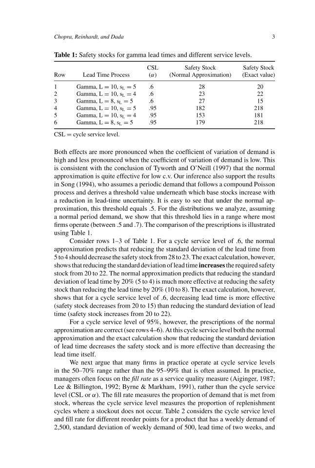
Table 1: Safety stocks for gamma lead times and different service levels.
CSL Safety Stock Safety StockRow Lead Time Process (α) (Normal Approximation) (Exact value)
1 Gamma, L = 10, sL = 5 .6 28 202 Gamma, L = 10, sL = 4 .6 23 223 Gamma, L = 8, sL = 5 .6 27 154 Gamma, L = 10, sL = 5 .95 182 2185 Gamma, L = 10, sL = 4 .95 153 1816 Gamma, L = 8, sL = 5 .95 179 218
CSL = cycle service level.
Both effects are more pronounced when the coefficient of variation of demand ishigh and less pronounced when the coefficient of variation of demand is low. Thisis consistent with the conclusion of Tyworth and O’Neill (1997) that the normalapproximation is quite effective for low c.v. Our inference also support the resultsin Song (1994), who assumes a periodic demand that follows a compound Poissonprocess and derives a threshold value underneath which base stocks increase witha reduction in lead-time uncertainty. It is easy to see that under the normal ap-proximation, this threshold equals .5. For the distributions we analyze, assuminga normal period demand, we show that this threshold lies in a range where mostfirms operate (between .5 and .7). The comparison of the prescriptions is illustratedusing Table 1.
Consider rows 1–3 of Table 1. For a cycle service level of .6, the normalapproximation predicts that reducing the standard deviation of the lead time from5 to 4 should decrease the safety stock from 28 to 23. The exact calculation, however,shows that reducing the standard deviation of lead time increases the required safetystock from 20 to 22. The normal approximation predicts that reducing the standarddeviation of lead time by 20% (5 to 4) is much more effective at reducing the safetystock than reducing the lead time by 20% (10 to 8). The exact calculation, however,shows that for a cycle service level of .6, decreasing lead time is more effective(safety stock decreases from 20 to 15) than reducing the standard deviation of leadtime (safety stock increases from 20 to 22).
For a cycle service level of 95%, however, the prescriptions of the normalapproximation are correct (see rows 4–6). At this cycle service level both the normalapproximation and the exact calculation show that reducing the standard deviationof lead time decreases the safety stock and is more effective than decreasing thelead time itself.
We next argue that many firms in practice operate at cycle service levelsin the 50–70% range rather than the 95–99% that is often assumed. In practice,managers often focus on the fill rate as a service quality measure (Aiginger, 1987;Lee & Billington, 1992; Byrne & Markham, 1991), rather than the cycle servicelevel (CSL or α). The fill rate measures the proportion of demand that is met fromstock, whereas the cycle service level measures the proportion of replenishmentcycles where a stockout does not occur. Table 2 considers the cycle service leveland fill rate for different reorder points for a product that has a weekly demand of2,500, standard deviation of weekly demand of 500, lead time of two weeks, and
4 The Effect of Lead Time Uncertainty on Safety Stocks
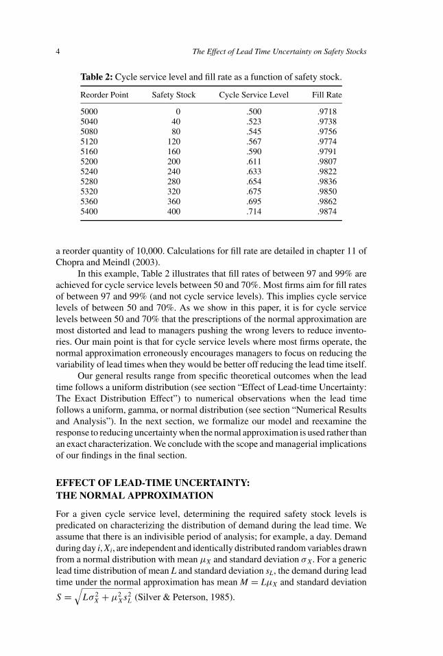
Table 2: Cycle service level and fill rate as a function of safety stock.
Reorder Point Safety Stock Cycle Service Level Fill Rate
5000 0 .500 .97185040 40 .523 .97385080 80 .545 .97565120 120 .567 .97745160 160 .590 .97915200 200 .611 .98075240 240 .633 .98225280 280 .654 .98365320 320 .675 .98505360 360 .695 .98625400 400 .714 .9874
a reorder quantity of 10,000. Calculations for fill rate are detailed in chapter 11 ofChopra and Meindl (2003).
In this example, Table 2 illustrates that fill rates of between 97 and 99% areachieved for cycle service levels between 50 and 70%. Most firms aim for fill ratesof between 97 and 99% (and not cycle service levels). This implies cycle servicelevels of between 50 and 70%. As we show in this paper, it is for cycle servicelevels between 50 and 70% that the prescriptions of the normal approximation aremost distorted and lead to managers pushing the wrong levers to reduce invento-ries. Our main point is that for cycle service levels where most firms operate, thenormal approximation erroneously encourages managers to focus on reducing thevariability of lead times when they would be better off reducing the lead time itself.
Our general results range from specific theoretical outcomes when the leadtime follows a uniform distribution (see section “Effect of Lead-time Uncertainty:The Exact Distribution Effect”) to numerical observations when the lead timefollows a uniform, gamma, or normal distribution (see section “Numerical Resultsand Analysis”). In the next section, we formalize our model and reexamine theresponse to reducing uncertainty when the normal approximation is used rather thanan exact characterization. We conclude with the scope and managerial implicationsof our findings in the final section.
EFFECT OF LEAD-TIME UNCERTAINTY:THE NORMAL APPROXIMATION
For a given cycle service level, determining the required safety stock levels ispredicated on characterizing the distribution of demand during the lead time. Weassume that there is an indivisible period of analysis; for example, a day. Demandduring day i, Xi, are independent and identically distributed random variables drawnfrom a normal distribution with mean µX and standard deviation σ X . For a genericlead time distribution of mean L and standard deviation sL, the demand during leadtime under the normal approximation has mean M = LµX and standard deviation
S =√
Lσ 2X + µ2
X s2L (Silver & Peterson, 1985).
Chopra, Reinhardt, and Dada 5
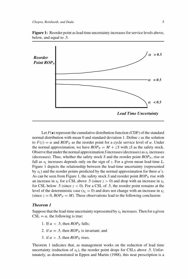
Figure 1: Reorder point as lead time uncertainty increases for service levels above,below, and equal to .5.
Reorder Point ROPN
Lead Time Uncertainty
α > 0.5
α = 0.5
α < 0.5
Let F(•) represent the cumulative distribution function (CDF) of the standardnormal distribution with mean 0 and standard deviation 1. Define z as the solutionto F(z) = α and ROPN as the reorder point for a cycle service level of α. Underthe normal approximation, we have ROPN = M + zS with zS as the safety stock.Observe that under the normal approximation S increases (decreases) as sL increases(decreases). Thus, whether the safety stock S and the reorder point ROPN , rise orfall as sL increases depends only on the sign of z. For a given mean lead-time L,Figure 1 depicts the relationship between the lead-time uncertainty (representedby sL) and the reorder points predicted by the normal approximation for three α’s.As can be seen from Figure 1, the safety stock S and reorder point ROPN rise withan increase in sL for a CSL above .5 (since z > 0) and drop with an increase in sL
for CSL below .5 (since z < 0). For a CSL of .5, the reorder point remains at thelevel of the deterministic case (sL = 0) and does not change with an increase in sL
(since z = 0, ROPN = M). These observations lead to the following conclusion:
Theorem 1
Suppose that the lead-time uncertainty represented by sL increases. Then for a givenCSL = α, the following is true:
1. If α < .5, then ROPN falls;
2. if α = .5, then ROPN is invariant; and
3. if α > .5, then ROPN rises.
Theorem 1 indicates that, as management works on the reduction of lead timeuncertainty (reduction of sL), the reorder point drops for CSLs above .5. Unfor-tunately, as demonstrated in Eppen and Martin (1988), this neat prescription is a
6 The Effect of Lead Time Uncertainty on Safety Stocks
consequence of the normal approximation. In the next section, we show the exis-tence of a threshold α > 0.5 such that for CSLs in [.5, α], the reorder point andsafety stock actually increase as sL decreases.
EFFECT OF LEAD-TIME UNCERTAINTY:THE EXACT DISTRIBUTION
In this section, we show how the prescriptions of the normal approximation inTheorem 1 are flawed for the case when periodic demand follows the normaldistribution and the lead time has a discrete uniform distribution with a meanof Y and a range of Y ± y. Denote the reorder point by R and let Gy(R) be the(unconditional) probability that demand during the lead time is less than or equal toR when the lead time is uniformly distributed between Y ± y. If µx is the expecteddemand per period and σ x is the standard deviation of demand per period, wedefine
zY (R) = (R − Yµx )/(σx
√Y ). (1)
It is clear from the definition of zY (R) that it represents the number of standarddeviations R is away from the expected value of demand given that the lead timeis Y . Let F(zY (R)) represent the probability that the standard normal is less than orequal to zY (R). As in Eppen and Martin (1988) it then follows that
G y(R) =(
1
2y + 1
) Y+y∑W=Y−y
F(zW (R)). (2)
From (1) and (2), it thus follows that
G y(R1) > G y(R2) if and only if R1 > R2. (3)
Observe that the case when y = 0 corresponds to the case of determinis-tic lead time. We are interested in examining how Gy(R) behaves as the leadtime uncertainty represented by y changes. We begin by examining the effectof increasing uncertainty by increasing y by one period. Then, simple algebrayields:
G y+1(R) − G y(R) =(
1
2y + 3
)[F(zY+y+1(R)) + F(zY−y−1(R)) − 2G y(R)],
(4)
and
G y+1(R) =(
2y + 1
2y + 3
)G y(R) +
(1
2y + 3
)[F(zY+y+1(R)) + F(zY−y−1(R))].
(5)
Since Y + y + 1 > Y − y − 1 ≥ 0, it readily follows that zY−y−1(R) ≥ zY+y+1(R),so that
1 > F(zY−y−1(R)) > F(zY+y+1(R)) > 0. (6)
Chopra, Reinhardt, and Dada 7
Our objective for the rest of the section is to try to come up with an analogue toFigure 1 for the case when we use the exact distribution of demand during the leadtime—shown in (2). To proceed we need the following lemma.
Lemma 1
Let Ry and Ry+1 be such that G y(Ry) = G y+1(Ry+1) = α. We have Ry+1 >
(<) Ry if and only if F(zY+y+1(Ry)) + F(zY−y−1(Ry)) < (>) 2G y(Ry).
Proof
Observe that if F(zY+y+1(Ry)) + F(zY−y−1(Ry)) < (>) 2G y(Ry), we haveG y+1(Ry) < (>) G y(Ry) = α by (3.4). Since G y+1(Ry+1) = α, using (3.3) wethus have Ry+1 > (<) Ry .
On the other hand, if Ry+1> (<) Ry , (3) implies that α = G y+1(Ry+1) >
(<) G y+1(Ry). Since α = G y(Ry), we have G y(Ry) > (<) G y+1(Ry). From (4)we thus have F(zY+y+1(Ry)) + F(zY−y−1(Ry)) < (>) 2G y(Ry). The result thusfollows. Another result needed is presented below. The proof follows from thedefinition of the standard normal distribution.
Lemma 2
Let F(·) be the standard normal cumulative distribution function. If z1 < 0 < z2,then 1 < F(z1) + F(z2) if and only if −z1 < z2.
We start by considering the reorder point as y increases for the case where theCSL is .5. For a given value of lead time uncertainty y, let Ry(0.5) be the reorderpoint such that G y(Ry(0.5)) = .5. For the case y = 0, observe that Ry(0.5) is theexpected demand, M = Yµx , during the lead time Y. We have zY+1(R0(0.5)) <
0 < −zY+1(R0(0.5)) < zY−1(R0(0.5)) from (1). From Lemma 2 it thus followsthat F(zY+1(R0(0.5))) + F(zY−1(R0(0.5))) > 2G0(R0(0.5)) = 1. Using Lemma 1it thus follows that R1(0.5) < R0(0.5).
In other words, the reorder point decreases as lead time uncertainty increasesfrom y = 0 to y = 1 for a cycle service level of .5. In the next result we provethat this pattern continues to hold as lead time uncertainty (y) increases, that is, thereorder point continues to drop as lead time uncertainty (y) increases for a cycleservice level of .5.
Theorem 2
For a cycle service level α = .5, the reorder point Ry(0.5) declines with an increasein lead time uncertainty y, that is, Ry+1(0.5) < Ry(0.5).
Theorem 2 (proved in the appendix) is equivalent to stating that the medianof the distribution of demand during the lead time declines as lead time uncertaintyrepresented by y increases. In contrast, the median is invariant when the normalapproximation is used. For the specific case of the median, Theorem 2 providesa complete characterization of the behavior of the reorder point as y increases. Ingeneral, the reorder point is the solution to
G y(R) =(
1
2y + 1
) Y+y∑W=Y−y
F(zW (R)) = α. (7)
8 The Effect of Lead Time Uncertainty on Safety Stocks
Let Ry(α) represent the unique solution to (7). To examine the effect of increasingthe cycle service level α it is sufficient to specialize (4) to:
G y+1(Ry(α)) − G y(Ry(α))
=(
1
2y + 3
)[F(zY+y(Ry(α))) + F(zY−y(Ry(α))) − 2α] (8)
Observe that Theorem 2 implicitly analyzes (8) for the special case α =.5. By Lemma 1, for arbitrary α, determining whether the reorder point in-creases or decreases depends on the sign of the term 2α − [F(zY+y(Ry(α))) +F(zY−y(Ry(α)))].
Theorem 3
1. If 0 < α < .5, there exists y > 0 such that Ry(α) < R0(α);
2. There exists .5 < α < 1 and y > 0 such that Ry (α) < R0 (α).
Part 1 of this theorem states that the optimal reorder point falls with increasinguncertainty if the CSL is less than .5. Part 2 states that there are service levelsα > .5 for which the reorder point initially falls with an increase in lead timeuncertainty, which contradicts the prediction for the normal approximation. Weprove both parts in the Appendix.
In the next section we numerically study the effect of decreasing lead timeuncertainty on safety stocks for various lead time distributions.
NUMERICAL RESULTS AND ANALYSIS
Theorems 2 and 3 show that there is a range of cycle service levels above 50% wheredecreasing the lead time uncertainty increases the reorder point and safety stockwhen the lead time is uniformly distributed. In this section we present computationalevidence to show that these claims are valid when lead times follow the gamma, theuniform, or the normal distribution. For the gamma lead time distribution we showthat for cycle service levels around 60%, decreasing lead time variability increasesthe reorder point. For the uniform lead time this effect is observed for cycle servicelevels close to, but above, 50%. As we have discussed earlier, most firms operateat cycle service levels in this range because they imply fill rates of around 98%.Using the computational results we also show that in this range, a manager is betteroff decreasing lead time rather than lead time variability if reducing inventories isthe goal.
We first consider the effect of reducing lead time variability on reorder pointsand safety stock when the lead time follows the uniform or gamma distribution.In both cases we keep the mean lead time fixed and vary the standard deviation.Demand per period is assumed to be normal with a mean µ = 20 and standarddeviation σ = 15 or 5. This allows us to analyze the effect for both a high and lowcoefficient of variation of demand.
Figure 2 shows the effect of reducing lead time variability when periodicdemand has a high coefficient of variation (15/20) and lead time is uniformlydistributed with a mean of 10 and a range of 10 ± y, where y ranges from
Chopra, Reinhardt, and Dada 9
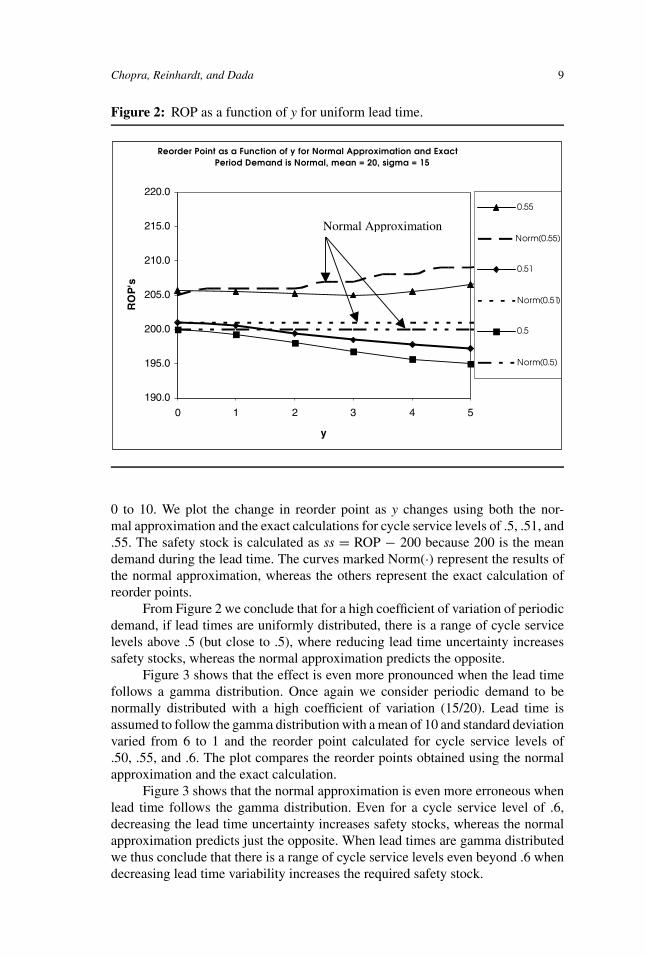
Figure 2: ROP as a function of y for uniform lead time.
Reorder Point as a Function of y for Normal Approximation and ExactPeriod Demand is Normal, mean = 20, sigma = 15
190.0
195.0
200.0
205.0
210.0
215.0
220.0
0 1 2 3 4 5
y
RO
P's
0.55
Norm(0.55)
0.51
Norm(0.51)
0.5
Norm(0.5)
Normal Approximation
0 to 10. We plot the change in reorder point as y changes using both the nor-mal approximation and the exact calculations for cycle service levels of .5, .51, and.55. The safety stock is calculated as ss = ROP − 200 because 200 is the meandemand during the lead time. The curves marked Norm(·) represent the results ofthe normal approximation, whereas the others represent the exact calculation ofreorder points.
From Figure 2 we conclude that for a high coefficient of variation of periodicdemand, if lead times are uniformly distributed, there is a range of cycle servicelevels above .5 (but close to .5), where reducing lead time uncertainty increasessafety stocks, whereas the normal approximation predicts the opposite.
Figure 3 shows that the effect is even more pronounced when the lead timefollows a gamma distribution. Once again we consider periodic demand to benormally distributed with a high coefficient of variation (15/20). Lead time isassumed to follow the gamma distribution with a mean of 10 and standard deviationvaried from 6 to 1 and the reorder point calculated for cycle service levels of.50, .55, and .6. The plot compares the reorder points obtained using the normalapproximation and the exact calculation.
Figure 3 shows that the normal approximation is even more erroneous whenlead time follows the gamma distribution. Even for a cycle service level of .6,decreasing the lead time uncertainty increases safety stocks, whereas the normalapproximation predicts just the opposite. When lead times are gamma distributedwe thus conclude that there is a range of cycle service levels even beyond .6 whendecreasing lead time variability increases the required safety stock.
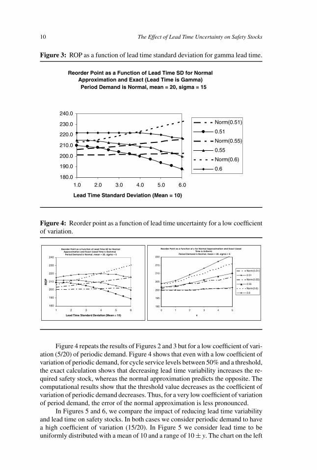
10 The Effect of Lead Time Uncertainty on Safety Stocks
Figure 3: ROP as a function of lead time standard deviation for gamma lead time.
Reorder Point as a Function of Lead Time SD for Normal Approximation and Exact (Lead Time is Gamma)Period Demand is Normal, mean = 20, sigma = 15
180.0
190.0
200.0
210.0
220.0
230.0
240.0
1.0 2.0 3.0 4.0 5.0 6.0
Lead Time Standard Deviation (Mean = 10)
Norm(0.51)
0.51
Norm(0.55)
0.55
Norm(0.6)
0.6
Figure 4: Reorder point as a function of lead time uncertainty for a low coefficientof variation.
Reorder Point as a Function of Lead Time SD for Normal Approximation and Exact (Lead Time is Gamma)
Period Demand is Normal, mean = 20, sigma = 5
180
190
200
210
220
230
240
1 2 3 4 5 6
Lead Time Standard Deviation (Mean = 10)
RO
P
Reorder Point as a Function of y for Normal Approximation and Exact (Lead Time is Uniform)
Period Demand is Normal, mean = 20, sigma = 5
190
195
200
205
210
215
220
0 1 2 3 4 5
y
Norm(0.51)
0.51
Norm(0.55)
0.55
Norm(0.6)
0.6
Figure 4 repeats the results of Figures 2 and 3 but for a low coefficient of vari-ation (5/20) of periodic demand. Figure 4 shows that even with a low coefficient ofvariation of periodic demand, for cycle service levels between 50% and a threshold,the exact calculation shows that decreasing lead time variability increases the re-quired safety stock, whereas the normal approximation predicts the opposite. Thecomputational results show that the threshold value decreases as the coefficient ofvariation of periodic demand decreases. Thus, for a very low coefficient of variationof period demand, the error of the normal approximation is less pronounced.
In Figures 5 and 6, we compare the impact of reducing lead time variabilityand lead time on safety stocks. In both cases we consider periodic demand to havea high coefficient of variation (15/20). In Figure 5 we consider lead time to beuniformly distributed with a mean of 10 and a range of 10 ± y. The chart on the left
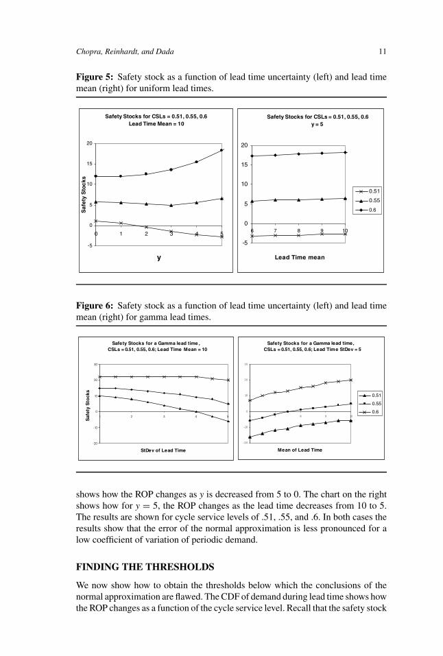
Chopra, Reinhardt, and Dada 11
Figure 5: Safety stock as a function of lead time uncertainty (left) and lead timemean (right) for uniform lead times.
Safety Stocks for CSLs = 0.51, 0.55, 0.6y = 5
-5
0
5
10
15
20
6 7 8 9 10
Lead Time mean
0.51
0.55
0.6
Safety Stocks for CSLs = 0.51, 0.55, 0.6 Lead Time Mean = 10
-5
0
5
10
15
20
0 1 2 3 4 5
y
Saf
ety
Sto
cks
Figure 6: Safety stock as a function of lead time uncertainty (left) and lead timemean (right) for gamma lead times.
Safety Stocks for a Gamma lead time ,CSLs = 0.51, 0.55, 0.6; Lead Time Mean = 10
-20
-10
0
10
20
30
1 2 3 4 5
StDev of Lead Time
Saf
ety
Sto
cks
Safety Stocks for a Gamma lead time, CSLs = 0.51, 0.55, 0.6; Lead Time StDev = 5
-20
-10
0
10
20
30
6 7 8 9 10
Mean of Lead Time
0.51
0.55
0.6
shows how the ROP changes as y is decreased from 5 to 0. The chart on the rightshows how for y = 5, the ROP changes as the lead time decreases from 10 to 5.The results are shown for cycle service levels of .51, .55, and .6. In both cases theresults show that the error of the normal approximation is less pronounced for alow coefficient of variation of periodic demand.
FINDING THE THRESHOLDS
We now show how to obtain the thresholds below which the conclusions of thenormal approximation are flawed. The CDF of demand during lead time shows howthe ROP changes as a function of the cycle service level. Recall that the safety stock
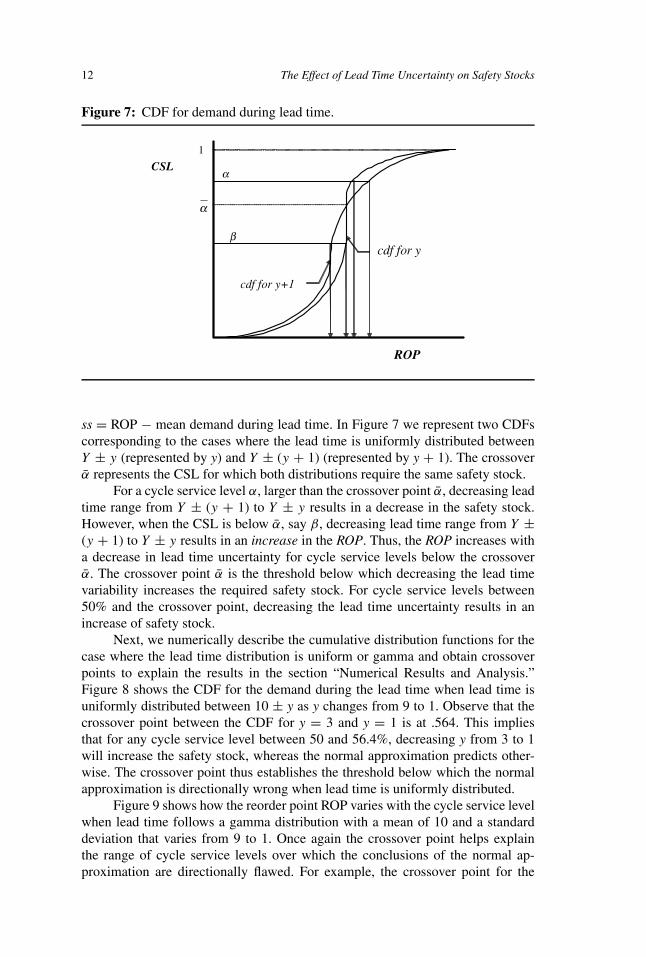
12 The Effect of Lead Time Uncertainty on Safety Stocks
Figure 7: CDF for demand during lead time.
CSL
ROP
1
α
cdf for y+1
cdf for y
α
β
ss = ROP − mean demand during lead time. In Figure 7 we represent two CDFscorresponding to the cases where the lead time is uniformly distributed betweenY ± y (represented by y) and Y ± (y + 1) (represented by y + 1). The crossoverα represents the CSL for which both distributions require the same safety stock.
For a cycle service level α, larger than the crossover point α, decreasing leadtime range from Y ± (y + 1) to Y ± y results in a decrease in the safety stock.However, when the CSL is below α, say β, decreasing lead time range from Y ±(y + 1) to Y ± y results in an increase in the ROP. Thus, the ROP increases witha decrease in lead time uncertainty for cycle service levels below the crossoverα. The crossover point α is the threshold below which decreasing the lead timevariability increases the required safety stock. For cycle service levels between50% and the crossover point, decreasing the lead time uncertainty results in anincrease of safety stock.
Next, we numerically describe the cumulative distribution functions for thecase where the lead time distribution is uniform or gamma and obtain crossoverpoints to explain the results in the section “Numerical Results and Analysis.”Figure 8 shows the CDF for the demand during the lead time when lead time isuniformly distributed between 10 ± y as y changes from 9 to 1. Observe that thecrossover point between the CDF for y = 3 and y = 1 is at .564. This impliesthat for any cycle service level between 50 and 56.4%, decreasing y from 3 to 1will increase the safety stock, whereas the normal approximation predicts other-wise. The crossover point thus establishes the threshold below which the normalapproximation is directionally wrong when lead time is uniformly distributed.
Figure 9 shows how the reorder point ROP varies with the cycle service levelwhen lead time follows a gamma distribution with a mean of 10 and a standarddeviation that varies from 9 to 1. Once again the crossover point helps explainthe range of cycle service levels over which the conclusions of the normal ap-proximation are directionally flawed. For example, the crossover point for the
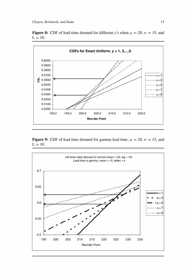
Chopra, Reinhardt, and Dada 13
Figure 8: CDF of lead time demand for different y’s when µ = 20, σ = 15, andL = 10.
CDFs for Exact Uniform, y = 1, 3,...,9
0.5000
0.5100
0.5200
0.5300
0.5400
0.5500
0.5600
0.5700
0.5800
0.5900
0.6000
190.0 195.0 200.0 205.0 210.0 215.0 220.0
Reorder Point
CS
L
y = 1
y = 3
y = 5
y = 7
y = 9
Figure 9: CDF of lead time demand for gamma lead time, µ = 20, σ = 15, andL = 10.
cdf when daily demand is normal (mean = 20, sig = 15)Lead time is gamma, mean = 10, stdev = s
0.5
0.55
0.6
0.65
0.7
195 200 205 210 215 220 225 230 235
Reorder Point
s = 1
s = 3
s = 5
s = 7
s = 9
14 The Effect of Lead Time Uncertainty on Safety Stocks
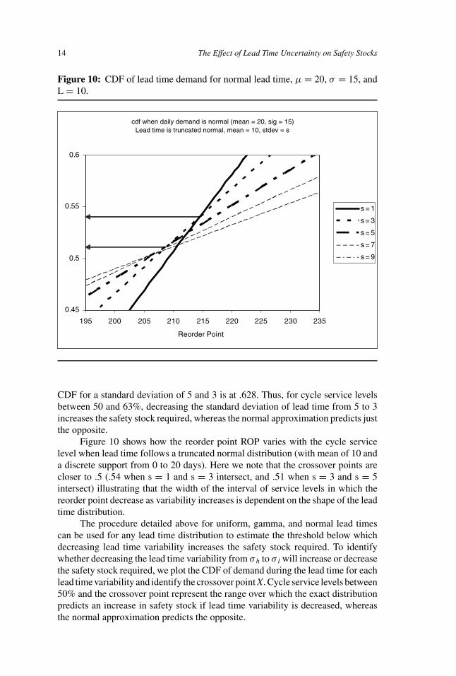
Figure 10: CDF of lead time demand for normal lead time, µ = 20, σ = 15, andL = 10.
cdf when daily demand is normal (mean = 20, sig = 15)Lead time is truncated normal, mean = 10, stdev = s
0.45
0.5
0.55
0.6
195 200 205 210 215 220 225 230 235
Reorder Point
s = 1
s = 3
s = 5
s = 7
s = 9
CDF for a standard deviation of 5 and 3 is at .628. Thus, for cycle service levelsbetween 50 and 63%, decreasing the standard deviation of lead time from 5 to 3increases the safety stock required, whereas the normal approximation predicts justthe opposite.
Figure 10 shows how the reorder point ROP varies with the cycle servicelevel when lead time follows a truncated normal distribution (with mean of 10 anda discrete support from 0 to 20 days). Here we note that the crossover points arecloser to .5 (.54 when s = 1 and s = 3 intersect, and .51 when s = 3 and s = 5intersect) illustrating that the width of the interval of service levels in which thereorder point decrease as variability increases is dependent on the shape of the leadtime distribution.
The procedure detailed above for uniform, gamma, and normal lead timescan be used for any lead time distribution to estimate the threshold below whichdecreasing lead time variability increases the safety stock required. To identifywhether decreasing the lead time variability from σ h to σ l will increase or decreasethe safety stock required, we plot the CDF of demand during the lead time for eachlead time variability and identify the crossover point X. Cycle service levels between50% and the crossover point represent the range over which the exact distributionpredicts an increase in safety stock if lead time variability is decreased, whereasthe normal approximation predicts the opposite.
Chopra, Reinhardt, and Dada 15
CONCLUSION
For the most part, management’s understanding of the effect on safety stocks ofuncertainty in lead time is based on an approximate characterization of demandduring lead time using the normal distribution. For cycle service levels above50% the normal approximation predicts that a manager can reduce safety stocks bydecreasing lead time uncertainty. Our analytical results and numerical experiments,however, indicate that for cycle service levels between 50% and a threshold, theprescriptions of the normal approximation are flawed, and decreasing the lead timeuncertainty, in fact, increases the required safety stock. In this range of cycle servicelevels, a manager who wants to decrease inventories should focus on decreasinglead times rather than lead time variability. This contradicts the conclusion drawnusing the normal approximation.
Our conclusion is more pronounced when demand has a high coefficient ofvariation. When the lead time follows a gamma distribution, the prescriptions ofthe normal approximation are flawed over a wide range of cycle service levels.This range is narrower when lead times are uniformly or normally distributed.Thus, using the normal approximation makes sense if lead times are normallydistributed, but it would not make sense if lead times follow a distribution closerto the gamma. [Received: February 2002. Accepted: October 2003.]
REFERENCES
Aiginger, K. (1987). Production and decision theory under uncertainty. London:Blackwell.
Byrne, P. M., & Markham, W. J. (1991). Improving quality and productivity in thelogistics process. Oak Brook, IL: Council of Logistics Management.
Chopra, S., & Meindl, P. (2003). Supply chain management: Strategy, planning,and operations (2nd ed.). New York: Prentice Hall.
Eppen, G. D., & Martin, R. K. (1988). Determining safety stock in the presence ofstochastic lead time and demand. Management Science, 34(11), 1380–1390.
Lee, H. L., & Billington, C. (1992). Managing supply chain inventory: Pitfalls andopportunities. Sloan Management Review, 33, 65–73.
Silver, E. A., & Peterson, R. (1985). Decision systems for inventory managementand production planning. New York: Wiley.
Song, J.-S. (1994). The effect of lead time uncertainty in a simple stochastic in-ventory model. Management Science, 40(5), 603–613.
APPENDIX A: PROOF OF THEOREMS 2 AND 3
To lighten notation throughout, we let c = σx/µx .
Theorem 2
For α = .5, the reorder point Ry(0.5) declines with an increase in lead time uncer-tainty y, that is, Ry+1(0.5) < Ry(0.5).

16 The Effect of Lead Time Uncertainty on Safety Stocks
Proof
The result is proved using induction. We first consider the case for y = 0, that is,the lead time is fixed at Y . For a fixed lead time Y, the reorder point for a cycleservice level of .5 is given by Ro(0.5) = Yµx .
Now consider the lead time to be uniformly distributed with equal supporton {Y + 1, Y, Y − 1}, that is, y = 1. If the reorder point is kept at R0(.5) = Yµx,the cycle service level is given by
1
3
{F
((Y − (Y − 1))
c√
Y − 1
)+ F
((Y − (Y + 1))
c√
Y + 1
)+ F
((Y − Y )
c√
Y
)}
We claim that F( 1c√
Y − 1) + F( −1
c√
Y + 1) > 1. By Lemma 2, this follows because
−1c√
Y + 1< 0 < 1
c√
Y − 1and 1
c√
Y + 1< 1
c√
Y − 1. This implies that if y = 1, the cycle
service level for a reorder point of R0(.5) is strictly greater than .5. Thus, R1(.5) <
R0(.5). Define �1 = (R0(.5) − R1(.5))/µx. The service level at R1(.5) is .5 and isgiven by
1
3
{F
((Y − (Y − 1)) − �1
c√
Y − 1
)+ F
((Y − (Y + 1)) − �1
c√
Y + 1
)
+ F
((Y − Y ) − �1√
Y
)}= 0.5. (A1)
Since �1 > 0, we have F(−�1
c√
Y) < 0.5.Thus, it must be the case that
F
(1 − �1
c√
Y − 1
)+ F
(−1 − �1
c√
Y + 1
)> 1 or by Lemma 2
1 − �1
c√
Y − 1>
1 + �1
c√
Y + 1. (A2)
Now consider raising the lead time uncertainty by assuming lead time to be uni-formly distributed over {Y − 2, Y − 1, Y , Y + 1, Y + 2}. If the reorder point iskept at R1(.5) = Yµx − �1µx, the cycle service level is given by
1
5
{F
((Y − (Y − 2)) − �1
c√
Y − 2
)+ F
((Y − (Y + 2)) − �1
c√
Y + 2
)
+ F
((Y − (Y − 1)) − �1
c√
Y − 1
)+ F
((Y − (Y + 1)) − �1
c√
Y + 1
)
+ F
((Y − Y ) − �1√
Y
)}
We now claim that F( 2 − �1
c√
Y − 2) + F(−2 − �1
c√
Y + 2) > 1.
By Lemma 2, this is equivalent to showing that
2 − �1
c√
Y − 2= 1
c√
Y − 2+ 1 − �1
c√
Y − 2>
2 + �1
c√
Y + 2= 1
c√
Y + 2+ 1 + �1
c√
Y + 2.
(A3)

Chopra, Reinhardt, and Dada 17
From (A2), we have
1 − �1
c√
Y − 2>
1 − �1
c√
Y − 1>
1 + �1
c√
Y + 1>
1 + �1
c√
Y + 2.
Given the fact that 1c√
Y − 2> 1
c√
Y + 2, (A3) thus follows. This implies that if y = 2,
the cycle service level for a reorder point of R1(.5) is strictly greater than .5. Thus,R2(.5) < R1(.5). Define �2 = (R1(.5) − R2(.5))/µx.
We now use induction to complete the proof. Define �y = (Ry−1(.5) −Ry(.5))/µx. To show that Ry+1(.5) < Ry(.5) we start with the induction as-sumption that y − �y
c√
Y − y>
y + �y
c√
Y + y. We now need to prove that F( y + 1 − �y
c√
Y − (y + 1)) +
F(−(y + 1) − �y
c√
Y + (y + 1)) > 1.
Observe that
(y + 1) − �y
c√
Y − (y + 1)= y
c√
Y − (y + 1)+ 1 − �y
c√
Y − (y + 1)
>y
c√
Y − (y + 1)+ 1 − �y
c√
Y − y
>y
c√
Y + (y + 1)+ 1 + �y
c√
Y + y
> {This follows from the induction hypothesis}
y
c√
Y + (y + 1)+ 1 + �y
c√
Y + (y + 1)= (y + 1) + �y
c√
Y + (y + 1).
The result thus follows using Lemma 2. This implies that Ry+1(.5) < Ry(.5).
Theorem 3, Part 1
If 0 < α ≤ .5, there exists a y > 0 such that Ry(α) < R0(α).
Proof
If the lead time is fixed at Y , the cycle service level for a reorder point of Rµx (R ∈(0, Y )) is given by F( R − Y
c√
Y). Consider now lead time to be uniformly distributed
on {Y − y, Y , Y + y} where y is some small positive value. We show that the cycleservice level under this setting (with the reorder point fixed at Rµx) increases, orequivalently
F
(R − (Y + y)
c√
Y + y
)+ F
(R − (Y − y)
c√
Y − y
)> 2F
(R − Y
c√
Y
)(A4)
for some y > 0. By Lemma 1, this is equivalent to proving

18 The Effect of Lead Time Uncertainty on Safety Stocks
R − (Y + y)
c√
Y + y+ R − (Y − y)
c√
Y − y> 2
R − Y
c√
Y
or
R − Y
c√
Y− R − (Y + y)
c√
Y + y<
R − (Y − y)
c√
Y − y− R − Y
c√
Y.
This inequality is equivalent to
(R − Y )(2√
Y + y√
Y − y −√
Y√
Y − y −√
Y√
Y + y)
< y(√
Y√
Y + y −√
Y√
Y − y).
Observe that the right-hand side is clearly positive and (R − Y ) is nonpositive byassumption and thus maximized at R = 0. Therefore, it remains to show that
(−Y )(2√
Y + y√
Y − y −√
Y√
Y − y −√
Y√
Y + y)
< y(√
Y√
Y + y −√
Y√
Y − y).
Without loss of generality, assume that y = βY for some β ∈ [0, 1].
Basic algebraic manipulations yield
√1 − β
√1 + β
(√1 + β − 1
)<
√1 − β
√1 + β
(1 −
√1 − β
)
or
√1 + β +
√1 − β < 2 which is true for β ∈ [0, 1].
Theorem 3, Part 2
There exist α > 0.5 and y > 0 such that Ry (α) < R0 (α).
Proof
Observe that (A4) is tight when y = 0. Differentiating its left-hand side with respectto y yields
A = f
(R − Y + y
c√
Y − y
)c√
Y − y − (R − Y + y) −c2√
Y−y
c2(Y − y)
+ f
(R − Y − y
c√
Y + y
)−c√
Y + y − (R − Y − y) c2√
Y+y
c2(Y + y)
which simplifies to

Chopra, Reinhardt, and Dada 19
f
(R − Y + y
c√
Y − y
)Y − y + R
2c(Y − y)3/2− f
(R − Y − y
c√
Y + y
)Y + y + R
2c(Y + y)3/2
with f (·) being the density function of the standardized normal distribution. Weshow that A > 0 for a small positive y. Without loss of generality, assume thatR = (1 + γ )Y and y = βY for γ > 0 and 0 < β < γ . Substituting yields
A = f
((γ + β)Y
c√
Y (1 − β)
)(2 + γ − β)Y
2cY 3/2(1 − β)3/2− f
((γ − β)Y
c√
Y (1 + β)
)(2 + γ + β)Y
2cY 3/2(1 + β)3/2
= 1
2c√
2πY
[exp
(−k
(γ + β)2
1 − β
)2 + γ − β
(1 − β)3/2− exp
(−k
(γ − β)2
1 + β
)2 + γ + β
(1 + β)3/2
]
where
k = Y
2c2.
We rewrite A as
A =exp
( − k (γ −β)2
1 + β
)2c
√2πY
[exp
(k
{(γ − β)2
1 + β− (γ + β)2
1 − β
})2 + γ − β
(1 − β)3/2
− 2 + γ + β
(1 + β)3/2
].
To show that the above is nonnegative for a suitable k, we need to show that
exp
(k
{(γ − β)2
1 + β− (γ + β)2
1 − β
})2 + γ − β
(1 − β)3/2− 2 + γ + β
(1 + β)3/2≥ 0
for a small enough β. Thus A > 0 reduces to
exp
(−k
{4γβ + 2γ 2β + 2β3
1 − β2
})2 + γ − β
(1 + β)3/2− 2 + γ + β
(1 + β)3/2≥ 0. (A5)
For k ≤ 14γ + 4γ 2 , we have
−k
{4γβ + 2γ 2β + 2β3
1 − β2
}≥ − β
1 − β2
or
exp
(−k
{β(4γ + 2γ 2 + 2β2)
1 − β2
})≥ exp
(− β
1 − β2
).
(A5) is satisfied if for a small β > 0 we can show that
H (γ, β) = exp
(− β
1 − β2
)2 + γ − β
(1 − β)3/2− 2 + γ + β
(1 + β)3/2> 0. (A6)

20 The Effect of Lead Time Uncertainty on Safety Stocks
Since H (γ , 0) = 0 and 2 + γ +β
(1 +β)3/2 is decreasing in β, it remains to show that H 1 (γ ,β) is nondecreasing initially for a small positive β, where
H1(γ, β) = exp
(− β
1 − β2
)2 + γ − β
(1 − β)3/2.
We compute
∂ H1(γ, β)
∂β= exp
(− β
1 − β2
)−(1 − β)3/2 + 32 (2 + γ − β)
√1 − β
(1 − β)3
+ exp
(− β
1 − β2
)(2 + γ − β
(1 − β)3/2
)(−(1 − β)2 − 2β2
(1 − β2)2
)
At β = 0,∂ H1(γ, β)
∂β
∣∣∣∣β=0
= −1 + 3
2(2 + γ ) − (2 + γ ) > 0
and by continuity we conclude that ∂ H1(γ,β)∂β
≥ 0 for a small positive β and therefore
H 1 (γ , β) is increasing initially. Thus, if k = Y2c2 ≤ 1
4γ + 4γ 2 the cycle service levelinitially increases with an increase in lead time uncertainty and the associatedreorder point decreases.
APPENDIX B: TECHNICAL METHODOLOGY
The Normal Approximation for the Exact Uniform Distribution
ROPN = F−1{α, µyµx ,
√µyσ
2X + y(y + 1)µ2
X/3} where F−1 {•, •, •} is theinverse of the normal distribution (NORMINV) of given mean and standarddeviation.
The Normal Approximation for the Gamma Distribution
ROPN = F−1{α, Lµx ,√
Lσ 2X + s2
Lµ2X} where F−1 {•, •, •} is the inverse of the
normal distribution of given mean and standard deviation and L and sL are the meanand standard deviation of the gamma distribution.
The Exact Uniform
Sheet 1. Generate Table indexed by (row) ROP and (column) y with CSL inthe body of the Table.
Sheet 2. Use VLOOKUP function to extract ROP index that corresponds togiven y and CSL.
The Discrete Gamma Distribution
We seek the inverse (G−1) of the cumulative distribution function of the demandduring lead time. The lead time distribution has mean L and standard deviation sL.We know

Chopra, Reinhardt, and Dada 21
ROP = G−1{P(D < X ) =∑
l=1,...,30
wl ∗ NORMDIST(X, l ∗ µX , σX ∗ sqrt(l), 1)}.
Sheet 1. Generate weights (wl, l = 1, . . . , 30) Table indexed by (row) support(between 0 and 30) and (column) standard deviation with, in row jand column s the value
GAMMADIST
(j,
(L
s
)2
,s2
L, 1
)
−j−1∑i=0
GAMMADIST
(i,
(L
s
)2
,s2
L, 1
)
for j = 1, . . . , 29 with 0 in row j = 0 and, in row j = 30,
GAMMADIST
(30,
(L
s
)2
,s2
L, 1
)
−29∑
i=0
GAMMADIST
(i,
(L
s
)2
,s2
L, 1
)
+ 1 −30∑
i=0
GAMMADIST
(i,
(L
s
)2
,s2
L, 1
).
That is, we add to j = 30 the mass of the tail to the right of 30. InSheet 1, we also generate a table of NORMDIST values as per theROP formula above.
Sheet 2. Matrix multiply the Sheet 1’s Normdist table to Sheet 1’s weightstable.
Sheet 3. Use a VLOOKUP(CSL) on Sheet 2 to find the ROP that yields thegiven CSL.
The resulting discrete gamma distributions for lead time are illustrated inFigure A1.
The Truncated Normal Distribution
We seek the inverse (G−1) of the cumulative distribution function of the demandduring lead time. The lead time distribution has mean L and standard deviation sL.We know
ROP = G−1{P(D < X ) =∑
l=1,...,L
wl ∗ NORMDIST(X, l ∗ µX , σX ∗ sqrt(l), 1)}.
Sheet 1. Generate weights Table indexed by (row) support (between 0 and30) and (column) standard deviation with, in row j and column s thevalue

22 The Effect of Lead Time Uncertainty on Safety Stocks
Figure A1: Gamma lead time distributions for standard deviations of 2.5, 5, 7.5,and 9.
Discrete Gamma, s = 2.5
0
0.02
0.04
0.06
0.08
0.1
0.12
0.14
0.16
0.18
1E-06 3 6 9 12 15 18 21 24 27 30
Support (Lead Time has mean = 10)
Discrete Gamma, s = 5
0
0.01
0.02
0.03
0.04
0.05
0.06
0.07
0.08
0.09
0.1
0 3 6 9 12 15 18 21 24 27 30
Support (Lead Time has mean = 10)
Theor. Mass
Discretized
Discrete Gamma, s = 7.5
0
0.01
0.02
0.03
0.04
0.05
0.06
0.07
0.08
1E-06 3 6 9 12 15 18 21 24 27 30
Support (Lead Time has mean = 10)
Discrete Gamma, s = 9
0
0.01
0.02
0.03
0.04
0.05
0.06
0.07
0.08
1E-06 3 6 9 12 15 18 21 24 27 30
Support (Lead Time has mean = 10)
NORMDIST( j, L , s, 1) −j−1∑i=0
NORMDIST(i, L , s, 1)
for j = 1, . . . , 29 with NORMDIST(0, L , s, 1) 0 in row
j = 0 and, in row j = 30,
NORMDIST(30, L , s, 1) −29∑
i=0
NORMDIST
(i,
(L
s
)2
,s2
L, 1
)
+ 1 −30∑
i=0
NORMDIST
(i,
(L
s
)2
,s2
L, 1
).
That is, we add to j = 0 and j = 30, respectively, the mass of the tailto the left of 0 and to the right of 30. In Sheet 1, we also generate atable of NORMDIST values as per the ROP formula above.
Sheet 2. Matrix multiply the Sheet 1’s Normdist table to Sheet 1’s weightstable.
Sheet 3. Use a VLOOKUP(CSL) on Sheet 2 to find the ROP that yields thegiven CSL.
Chopra, Reinhardt, and Dada 23
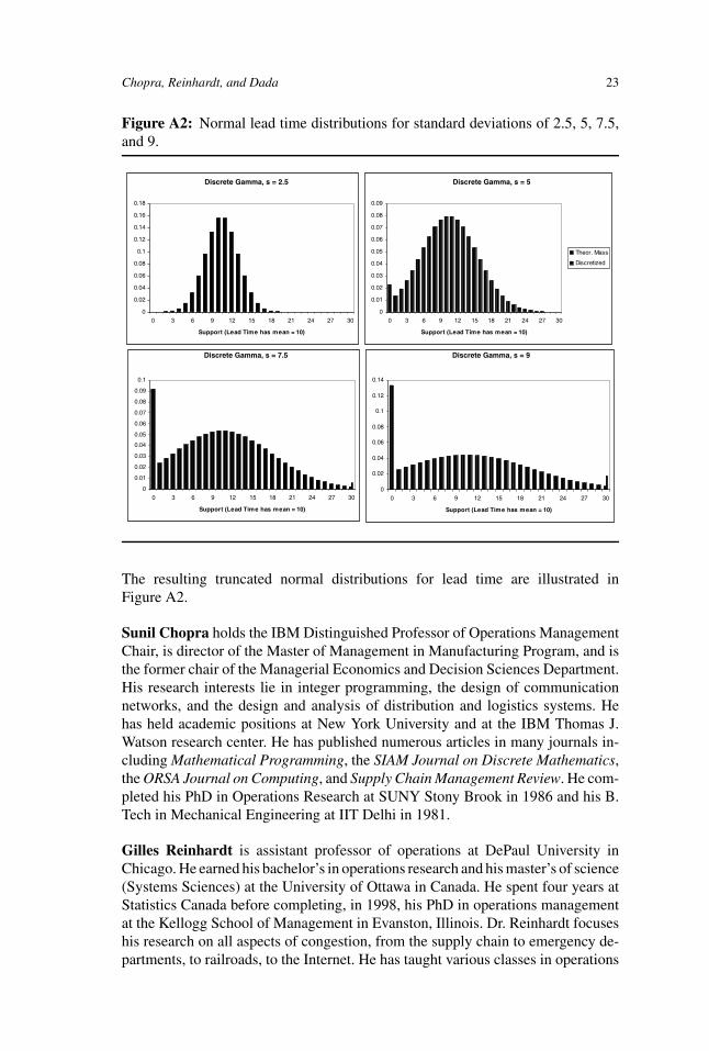
Figure A2: Normal lead time distributions for standard deviations of 2.5, 5, 7.5,and 9.
Discrete Gamma, s = 2.5
0
0.02
0.04
0.06
0.08
0.1
0.12
0.14
0.16
0.18
0 3 6 9 12 15 18 21 24 27 30
Support (Lead Time has mean = 10)
Discrete Gamma, s = 5
0
0.01
0.02
0.03
0.04
0.05
0.06
0.07
0.08
0.09
0 3 6 9 12 15 18 21 24 27 30
Support (Lead Time has mean = 10)
Theor. Mass
Discretized
Discrete Gamma, s = 7.5
0
0.01
0.02
0.03
0.04
0.05
0.06
0.07
0.08
0.09
0.1
0 3 6 9 12 15 18 21 24 27 30
Support (Lead Time has mean = 10)
Discrete Gamma, s = 9
0
0.02
0.04
0.06
0.08
0.1
0.12
0.14
0 3 6 9 12 15 18 21 24 27 30
Support (Lead Time has mean = 10)
The resulting truncated normal distributions for lead time are illustrated inFigure A2.
Sunil Chopra holds the IBM Distinguished Professor of Operations ManagementChair, is director of the Master of Management in Manufacturing Program, and isthe former chair of the Managerial Economics and Decision Sciences Department.His research interests lie in integer programming, the design of communicationnetworks, and the design and analysis of distribution and logistics systems. Hehas held academic positions at New York University and at the IBM Thomas J.Watson research center. He has published numerous articles in many journals in-cluding Mathematical Programming, the SIAM Journal on Discrete Mathematics,the ORSA Journal on Computing, and Supply Chain Management Review. He com-pleted his PhD in Operations Research at SUNY Stony Brook in 1986 and his B.Tech in Mechanical Engineering at IIT Delhi in 1981.
Gilles Reinhardt is assistant professor of operations at DePaul University inChicago. He earned his bachelor’s in operations research and his master’s of science(Systems Sciences) at the University of Ottawa in Canada. He spent four years atStatistics Canada before completing, in 1998, his PhD in operations managementat the Kellogg School of Management in Evanston, Illinois. Dr. Reinhardt focuseshis research on all aspects of congestion, from the supply chain to emergency de-partments, to railroads, to the Internet. He has taught various classes in operations

24 The Effect of Lead Time Uncertainty on Safety Stocks
management and quantitative analysis topics at undergraduate, MBA, and PhDlevels and has received awards for teaching excellence. He has presented papersat national and international conferences. He is an ad hoc referee for five journalsand has published in Computational Economics, Energy Studies Review, and theCanadian Journal of Emergency Medicine.
Maqbool Dada teaches operations management. His research interests includeinventory systems, pricing models, service systems, and international operationsmanagement. He has published articles in many journals including ManagementScience, Marketing Science, Operations Research, the European Journal ofOperational Research, and Interfaces. Prior to joining the Krannert (Purdue) fac-ulty in 1992, he was an assistant professor in the Department of Informationand Decision Sciences, College of Business Administration, at the University ofIllinois at Chicago. He has held visiting appointments at the Graduate School ofBusiness, University of Chicago, and at the Kellogg Graduate School of Manage-ment, Northwestern University. He completed his PhD in operations managementat the Massachusetts Institute of Technology in 1984 and his BS in IndustrialEngineering at Berkeley in 1978.