The Effect of Institutional Ownership on Payout Policy: A Regression

Discontinuity Design Approach

Alan D. Crane

Rice University

alan.d.crane@rice.edu

713-348-5393

Sébastien Michenaud

Rice University

michenaud@rice.edu

713-348-5935

James P. Weston

Rice University

westonj@rice.edu

713-348-4480

First Draft: 07/09/2012

This Draft: 12/13/2012

We thank David De Angelis, François Degeorge, François Derrien, Laurent Frésard, Gustavo Grullon,

Ambrus Kecskés, Andrew Koch, Alexander Ljungqvist, Garen Markarian, Brett Myers (discussant),

seminar participants at the CEPR European Summer Symposium in Financial Markets (Corporate Finance),

Lone Star Finance Symposium for helpful discussions, and Russell for providing the index data. All errors

are our own.

The Effect of Institutional Ownership on Payout Policy: A Regression

Discontinuity Design Approach

Abstract

We show that higher institutional ownership causes firms to pay more dividends and repurchase

more shares. Our identification strategy relies on a discontinuity in ownership based on the

annual composition of the Russell 1,000 and 2,000 indices. We also find evidence of a causal

effect on proxy voting, corporate investment, R&D, and equity issuance. Overall, results support

agency models where concentrated ownership lowers the marginal cost of delegated monitoring.

1

Institutional investors own the bulk of public equity in the US. Over the past 40 years,

ownership by institutions has increased dramatically from 10% in the 1970s to more than 60% by

2006 (Aghion, Van Reenen, Zingales (2012)). Testing whether differences in institutional

ownership influence corporate policy is important, but in practice it is very difficult to establish

causality. Not only do existing theories suggest different possible causal relationships, but also

the existing empirical evidence is mixed. While institutions may cause differences in corporate

policies, they may also choose stocks because of differences in corporate policy.

In this paper, we break the endogeneity between corporate policies and ownership by

showing that random ownership by institutions causes higher payout. Our identification of

causality relies on forced institutional holdings around the Russell 1000 and Russell 2000 index

cut-off to isolate a large discontinuity in institutional ownership. Each May 31st, the popular

Russell equity indices are formed based on stock market capitalizations. The largest 1,000 firms

are the Russell 1000 index while the next 2,000 make up the Russell 2000. The difference in size

around the Russell 1000/2000 cut-off is less than 2% of a standard deviation of daily returns.

Within some “bandwidth” around the cut-off, a firm's size ranking, and therefore index

assignment, is random. Since the indices are value-weighted, a firm ranked 1,000th in size has a

trivial weighting in the Russell 1000 while a firm ranked 1,001 is the largest stock in the Russell

2000 and must be held by any fund tracking or benchmarking against the index. Figure 1 shows

the weights for the firms in the Russell 1000 and the Russell 2000. From a tracking error

perspective, a firm's position just to the left or right of the threshold should have a significant

impact on ownership.

This discontinuity in the index composition represents random exposure to higher

institutional ownership that we exploit to test for causal effects on payout policy. Our main

finding is that more ownership by institutions appears to cause an increase in payout and a net

decrease in cash holdings. Specifically, we find that when randomly exposed to 9% higher

institutional ownership, firms pay 13% more in dividends, repurchase 22% more of their shares,

2

and on net pay out 5% more of their net cash flows. The effects we measure are consistent with

monitoring activity by institutional investors. We find that proxy-voting participation increases

by 55 percentage points for firms with higher institutional ownership. In the cross-section, our

results on payout policy are stronger for firms more likely to have high agency costs.

In a frictionless world, ownership shouldn’t matter (Miller and Modigliani (1961)). But

in the presence of frictions, there are some good reasons why it might. Jensen (1986) argues that

corporate managers are more likely to pay out free cash flow (rather than consume it) if the

marginal cost of delegated monitoring is lower. Admati, Pfleiderer, and Zechner (1994) argue

that as a firm’s shares become more widely held by less informed investors, the marginal benefits

of delegated monitoring decline and the costs increase. As a result, increased ownership by

institutions should increase the net returns to monitoring.

Institutional investors have long been associated with shareholder activism (see e.g.

Gillan and Starks, 2007), but even passive investors may help discipline managers and align

incentives with shareholders. For example, Edmans (2009), Admati, and Pfleiderer (2010), and

Edmans and Manso (2011) show passive investors may discipline managers through the threat of

exit. Further, institutions are generally required to participate in proxy votes by law.1 At a

minimum, ownership by institutions reduces coordination costs (Grossman and Hart (1980),

Shleifer and Vishny (1986)) and can lower agency costs through economies of scale in delegated

monitoring. Indeed, Brickley, Lease, and Smith (1988) find that voting on governance increases

with institutional ownership. Finally, Alexander et al. (2010) find that institutions often vote

based on the recommendations of proxy advisers such as Institutional Shareholder Services (ISS).

1 Proxy-voting is subject to the Employment Retirement Income Security Act (ERISA)’s fiduciary

responsibility rules for pension funds (1974), SEC’s Proxy-Voting by Investment Advisers rule (2003), and

SEC Rule 206(4)-6 of the Investment Advisers Act of 1940. Under these rules, pension funds and mutual

funds should vote their proxies in the best interests of their clients, i.e. to increase the value of the funds’

holdings.

3

Such behavior can increase coordinated voting, which can be pivotal in votes against

management.

Beyond agency costs, taxes and information asymmetry may also matter for payout

policy. Institutions are generally taxed less and better informed than individuals so they may

prefer to hold firms with certain payout and investment policies causing segmented clienteles of

ownership ((Barclay and Smith (1988), Brennan and Thakor (1990), Allen, Bernardo, and Welch

(2000)). These models often predict opposite causal relationships compared to monitoring

theories.

Consistent with the fundamental endogeneity between ownership structure and payout

policy, the empirical evidence is mixed. Allen and Michaely (2003) provide a comprehensive

survey of this large literature. They conclude that there is some limited evidence for tax-clientele

effects, little evidence in favor of signaling theories, and mixed evidence on agency theories.

Some recent studies have made progress on identifying causal channels between

ownership and payout policy.2 Even so, the evidence is still decidedly mixed. For example,

Grinstein and Michaely (2005) adopt a vector auto regression approach and find that institutions

are attracted to firms with positive payout but find no evidence that ownership Granger-causes

payouts. On the other hand, Gaspar, Massa, Matos, Patgiri and Rehman (2012) employ VARs in

a different setting and find the opposite. Desai and Jin (2011) show that plausibly exogenous

changes in payout policy cause changes in ownership by “dividend-averse” investors. Desai and

Jin (2011) and Perez Gonzales (2003) argue that exogenous changes in tax policy cause firms to

cater their payout policy to the tax preferences of their shareholders.3

2 Hartzell and Starks (2003) and Aghion, Van Reenen and Zingales (2012) use an instrumental variable

approach to study causal effects of institutional ownership on other corporate policies, specifically CEO

compensation and innovation, respectively. 3 In addition, Michaely, Thaler and Womack (1995) find no institutional ownership changes following

dividend omissions while Brav and Heaton (1998) find a drop in ownership around omissions after the

1974 ERISA regulations. Del Guercio (1996) finds a negative relationship between dividend yield and

mutual funds' portfolio choice.

4

Our identification strategy has distinct advantages relative to prior studies. First, our

setting has the advantage of not relying on institutional ownership changes for identification.

Changes in ownership are not random, and it is therefore difficult to rule out the possibility that

those changes are driven by unobservable determinants related to corporate policies (e.g.

expectations of future policies). Our setting rules out these unobservable factors causing payout.

As a result, while previous studies are limited only to Granger causality, we make a direct causal

interpretation.

Our approach is also distinct from past index inclusion studies (e.g. Pruitt and Wei

(1989)). Many index inclusion decisions are based on unobserved and potentially endogenous

decision rules. For example, a stock may be included in the S&P 500 because of some expected

changes in corporate policies or performance, or because institutional investors want to hold it.

In addition, while firms recently included in the S&P 500 index are observed, the firms that are

just outside are not. In contrast, our identification strategy relies on the (verifiable) assumption

that firms’ rankings around the Russell 1000/2000 threshold are random, and therefore so is the

exposure to higher institutional ownership associated with Russell 2000 index assignment.4

Chang and Hong (2012) also exploit this discontinuity and find that the smaller firms that

are just included in the more popular Russell 2000 index experience higher returns right after the

reconstitution of the index, which the authors attribute to price pressure due to higher institutional

demand for the Russell 2000 stocks.5 Consistent with their results, we find a large and significant

4 While firms could try to manipulate index inclusion at the threshold, as long as firms do not have precise

control over their assignment (which they don’t since they cannot precisely control their rank relative to

other firms), the discontinuity still identifies random assignment to the treatment, and the regression

discontinuity design is well specified (see e.g. Lee (2008) for a formal proof.) 5 They also document a significant increase in co-movement with other index stocks. In a previous version

of their paper, Chang and Hong also document a large change in institutional ownership around the

threshold. However, they also found a significant pre-treatment effect which violates the exogeneity of the

selection. In contrast, our sample selection procedure (detailed in section I.C) is specifically designed to

purge any pre-treatment effects.

5

exogenous discontinuity in a firm’s ownership structure, with firms at the top of the Russell 2000

having institutional ownership that is 9% greater than firms at the bottom of the Russell 1000.

Exposure to higher institutional ownership has an effect on corporate payout policy.

Firms at the top of the Russell 2000 pay $0.7M more in dividends over the next year and a

cumulated $1.5M over the next 3 years, which represents a 13% increase over the median

dividends for firms just in the Russell 1000. Share repurchases are also roughly $1M greater in

the next year, a 22% increase relative to the median, and total payout is about 5% larger. An

interesting aspect of our results is that they go against traditional size-based explanations: small

firms typically pay out less cash to shareholders, but in our case, arbitrarily smaller firms at the

discontinuity pay out more.

We also dig deeper into the cross-section to test whether our results are stronger for firms

that may benefit more from an increase in external monitoring. When we split the sample, we

find that the results are primarily driven by the firms with higher expected agency costs (low

profitability, high CEO compensation, low growth options). While these measures are imperfect,

they suggest payout is related to external monitoring. Furthermore, we find no differences based

on analyst coverage, suggesting that the effect may not stem from a change in information

asymmetry. The finding that proxy-voting participation increases by 55 percentage points around

the threshold reinforces our agency costs interpretation.

In addition to measures of net payout, we also test for changes in other corporate policies.

We find that higher institutional ownership causes an increase in net equity issues, total assets and

R&D expense. We find no significant treatment effects for capital expenditures, executive

compensation, profitability, or capital structure. While these results are mixed, they are generally

consistent with the idea that lower agency costs may increase corporate investment and that long-

run oriented institutional investors increase long-run R&D investment (Bushee (1998)).

We perform a battery of robustness tests. First, we replicate our results with alternative

measures and scaling variables. Second, we test the sensitivity of our results to regression

6

discontinuity methodology choices like bandwidth selection and kernel choice. Our results are

robust to alternative methodologies. Third, we find that lagged corporate policies do not exhibit a

discontinuity at the threshold, unlike policies after the change in index composition. This

suggests that our results are not driven by pre-treatment effects caused by selection bias in the

Russell index composition.6

Our paper makes several contributions. First, we provide evidence that institutional

ownership causes firms to disgorge cash. We don’t rule out that dividends cause changes in

ownership as in Grinstein and Michaely (2005), but we show that, in our setting, ownership

structure affects payout. Second, we show that institutions cause increases in investment and

equity issuance. Finally, consistent with Bond, Edmans, and Goldstein (2011), and Grullon,

Michenaud, and Weston (2012), we find evidence that capital market frictions, like random index

inclusion, can have an important impact on the economic behavior of publicly listed firms.

The paper is organized as follows. Section I briefly discusses the empirical strategies, the

data and the variables used in the tests. Section II presents the main empirical results, while

Section III discusses alternative explanations, robustness checks, and additional tests. Section IV

concludes.

I. Data and Methodology

A. Data

Our sample consists of the Russell 1000 and Russell 2000 index constituents from 1991

until 2008. These data are from Russell and are merged with firm level accounting data from

Compustat, institutional holdings data from Spectrum 13F filings, and stock return data from

CRSP. Our final sample includes 8,193 unique firms from 1991 to 2008. The average number of

years for which a firm is in either the Russell 1000 or 2000 in our sample is about 11 years.

6 Given the nature of the index inclusion rule, there is no selection bias for the inclusion in the indices. We

discuss selection issues related to the index weights assigned by Russell to firms in the index to adjust for

the level of investible shares in section I.C.

7

{Insert Table I about here}

Table I presents the summary statistics for our sample. Panel A shows statistics for the

Russell 1000 and Panel B shows the results for the Russell 2000. As expected, Russell 1000

firms (which are larger by definition) have a higher institutional ownership and have a higher

payout on average. As a result, these firms also have a lower percentage of assets held in cash

and tend to be more profitable with slightly higher leverage. In general, these results are

consistent with what we expect given a size-based classification of firms, and are particularly

useful for our identification strategy. We will see below that subsequent to index inclusion, at the

discontinuity, firms that are just in the smaller index - the Russell 2000 - pay out more of their

cash flows and hold less cash than the firms that are just in the larger index - the Russell 1000.

Therefore our results go against a purely size-based explanation.7

B. Regression Discontinuity Methodology

To measure the effect of the Russell index assignment on various firm policies, we

implement a regression discontinuity methodology similar to Imbens and Lemieux (2008) and

Lee and Lemieux (2010). The basic idea is that we have an exogenous discontinuous variable

that drives selection of observations into a treatment or control group around the discontinuity.

Assignment of observations to either the left or right of the discontinuity is random, at least near

the discontinuity. If this is the case, then we can measure a treatment effect by comparing data

from one side of the break-point to the other side. As long as assignment around the discontinuity

is not caused by any variable of interest prior to the assignment, then we can make causal

inference. Comparison of the data on either side of the discontinuity typically proceeds by some

form of local regression, on either side of the break-point, within some reasonably close

proximity.

7 We present a detailed discussion of pre- and post-treatment firm characteristics around the discontinuity

in section I.C.

8

In our setting, we argue that Russell index assignment is random close to the 1000/2000

threshold. Close to the 1,000th ranking, differences in market capitalization are very small (within

2% of a standard deviation of intraday return standard deviation) and so assignment to the left or

right of the break-point is essentially random. Since assignment is based on very small

differences in market capitalization rankings, it should be independent of firm characteristics

prior to the assignment. Given this setup, we can measure firm financial policies on both sides of

the threshold and test for any differences in those policies.

There are good reasons to expect differences around the 1000/2000 threshold. The

Russell 2000 is the most popular Russell index in terms of dollars benchmarked, meaning more

fund managers (and dollars) benchmark to the Russell 2000 index relative to the Russell 1000.

The Russell 1000 index competes against the popular S&P500 index for the large firms while the

Russell 2000 index faces less competition in mid to small cap stocks. Chang and Hong (2012)

report that in 2008 the amount of institutional assets benchmarked to the Russell 2000 index was

$264bn while only $169bn was benchmarked to the Russell 1000.

In addition, firms just included in the Russell 2000 have a large index weight while firms

just included in the Russell 1000 have only trivial portfolio weights. Figure 1 shows the

difference in index weights at the threshold. The largest firms in the Russell 2000 are likely to be

held by any fund tracking the Russell 2000 (even for actively managed funds) in order to keep

tracking error metrics reasonable. On the other hand, funds tracking the Russell 1000 could hold

none of the smallest firms in the index with no real impact on performance metrics. The

combination of the total benchmarked dollars and the difference in the relative index weights

motivates our prediction that institutional investors hold a larger proportion of firms just included

in the Russell 2000 and that this increase in institutional ownership is a function not of the

individual firms' characteristics, but rather the composition of the benchmarks.

Figure 1 shows the non-linear properties of the index weights around the threshold. As a

result, there are two main methodological choices we have to make in implementing the RDD

9

approach: how to define the neighborhood or bandwidth around the threshold and how to model

the local behavior of the data around the break-point. Our approach follows a standard sharp

regression discontinuity design format as described in Imbens and Lemieux (2008) and Roberts

and Whited (2012). As a starting point, we define the neighborhood around the discontinuity

using the Rule of Thumb (ROT) plug-in estimator (Fan and Gijbels (1996)). We then re-calculate

results over a continuum of bandwidths around this “optimal” neighborhood to check the

sensitivity of our estimates. In order to measure the treatment effect, we fit the data using semi-

nonparametric local polynomial regressions on each side of the threshold. Once we have

estimates for the expected value just-to-the left and just-to-the-right of the discontinuity, we can

test for differences and estimate the treatment effect. The details of our procedures, including our

optimal bandwidth selection, semi-nonparametric regression estimation, and standard errors are

described in Appendix 1.

C. Randomness of the Index Assignment and Float Adjustment

Our research design relies on the conditions of regression discontinuity being well

specified in our setting. However, there are number of adjustments made by Russell related to the

selection into the index and the subsequent determination of index weighting. These adjustments

have the potential to induce pre-treatment effects in our sample and violate our assumption of

randomness around the threshold. In this section, we describe the sample selection procedure we

use to mitigate any confounding effects of the adjustments made by Russell.

The Russell indices are constituted once every year using data as of May 31st each year,

and announced at the end of June. The Russell 1000 represents the 1,000 largest firms by market

value of equity and the Russell 2000 is the next 2,000 largest firms. The index constituents are

determined using market value ranks of the firms at the end of May where market values are

determined using closing share price and reported total shares outstanding.

10

Our identification relies on the notion that assignment to an index is random around the

1,000th rank threshold. In fact, the assignment to the index is based solely on the total market

capitalization of the firms at the end of May. As a result, a firm’s rank on May 31st, within a

certain range, should be orthogonal to firm policies. For example, it is possible for a firm to be

ranked 999 on May 30th, and 1001 on the 31st. This would lead to a different index assignment,

but is unlikely to be based on future expectations of financial policy. We can replicate the actual

Russell index assignment using only CRSP market capitalizations with 98% accuracy. While this

seems to satisfy our identification requirements, when we actually implement our regression tests

we must look at firms very close to the Russell 1000/2000 threshold, so any adjustment made by

Russell that affects firms close to the threshold may violate our assumption of randomness.

The first adjustment that Russell makes is to maintain consistency in the respective

indices. For example, if two firms on the edge of the threshold switch places in a given year,

Russell may leave those firms in their prior year index provided the market value differential is

small. This policy is coined “banding”, and according to Russell has not been applied

systematically prior to 2007. In our replication of the index assignments, we find that this affects

less than 1% of our sample. Nevertheless, our results do not change if we exclude data after

2007. This adjustment is easy to identify and does not appear to cause significant problems for

our discontinuity design.

The second adjustment made by Russell relates to the public float. Once each firm is

assigned to an index, Russell then assigns index weights based on market capitalization adjusted

for investible shares (e.g. treasury stock, block holders etc.). However, the investible shares data

are considered proprietary by Russell and are not made available to the public or the authors.

This adjustment can be large in some cases. Indeed, float adjustment by Russell may change the

ranks of firms relative to the threshold decision made based on unadjusted shares. For example,

if a Russell 1000 firm ranked very highly in terms of market capitalization has a large float

adjustment, the adjustment may push it near the threshold. If this happens, the largest firms in the

11

Russell 2000 may be different from those firms with the lowest weights in the Russell 1000. In

essence, we could find ourselves comparing firms that were not "neighbors" when the index

break-point was determined.

To address this issue, we first examine the nature of the float adjustment. While we

cannot directly observe the adjustment, we can easily proxy for it because we observe both the

adjusted and unadjusted weights. We calculate the percent difference between the unadjusted

weight and the adjusted weight used by Russell. We call this the weight prediction error and

large values indicate a large float adjustment. We find that firms with the lowest index weight in

the Russell 1000 have large float adjustments, and are persistently ranked at the lowest ranks of

the Russell 1000 index. This obviously introduces a problem of non-random proximity to the

threshold.

However, it is important to note that these adjustments are not related to our financial

policy variables of interest. Below, we report the results of a regression where we model the

weight prediction error (WPE) using lagged values of the error, stock returns (R), current and past

market values (MV), dummy variables for past inclusion in the index (I) and our corporate

variables of interest. We estimate the following relationship with T-statistics reported underneath

OLS point estimates:

1, , 1 , , ,[ 4.1] [20.6] [ 0.3] [1.7] [ 2.9]

2000, 1 2000, 2[3.2] [ 2.9]

1 1[0.43] [0.92]

0.045 0.83 0.20 4.0 6.0

0.04 0.03

0.4 0.3 ln( )

t ti t i t i April i April i April

Russell t Russell t

t t

WPE WPE R MV MV

I I

Volatility Dividends

1 1[0.16] [0.78]0.1 ln( ) 0.5 ln( )t tRepurchase Cash

We find that the weight prediction error is persistent and that the previous year's adjustment has

the largest effect on the current year. Beyond that, the only variables that contribute significantly

to this error are the size of the firm and the index assignment (1000 vs. 2000). These are

mechanical determinants in that larger firms within each index have large ranking errors. We

12

also see that the economic impact of these is small. A one standard deviation change in market

capitalization predicts a 0.004 standard deviation increase in the ranking error. More importantly,

we see that these ranking errors are not a significant function of any corporate policy variable.

While this adjustment by Russell should not invalidate our causal inferences (since it is

orthogonal to firm characteristics), we want to ensure there are no lingering selections biases that

might drive unknown pre-treatment effects for our sample. As a result, we simply drop

observations in the top 5% of squared ranking errors. The basic idea here is to identify the firms

that Russell has made a large share adjustment to, and remove them from the sample, while still

using the information in the actual index weights assigned by Russell, since it's the actual index

weights that drive institutional holdings8. Since we can identify the non-randomly selected firms

and remove them, we can hopefully ensure random characteristics around the threshold for the

remaining 95% of the sample.

To test whether the adjustments made by Russell leave any remaining selection bias

after our filter, we compare firm characteristics at the threshold before the index inclusion and

rank allocation by Russell. After excluding the 5% of observations with large adjustments, we

use the regression discontinuity methods described above to measure a variety of firm

characteristics to the right and the left of the threshold in the year prior to the index assignment.

If our filtered sample is random, we expect no pre-treatment effects in firm characteristics around

the threshold.

{Insert Table II about here}

Table II shows the results of these tests. Firms are very similar on both sides of the

threshold. The discontinuity tests show that there are no significant discontinuities around the

threshold in the prior year, suggesting there is no selection bias around the threshold.

8 Chang and Hong (2012) deal with this issue by using the unadjusted market weights. This makes sense

given the questions they address. In our setting, because the index weights are the underlying cause of the

institutional ownership and given the longer term nature of our tests, we feel our adjustment is appropriate.

However our payout results are qualitatively similar when using an unadjusted market weight ranking.

13

Importantly, there are no significant differences in institutional ownership, dividend policy, or

share repurchases. Our process of identifying and removing observations contaminated by the

Russell adjustment appears to preserve randomness around the threshold and ensure the

conditions for a regression discontinuity approach.

A final concern with our design is that some firms may have incentives to manipulate

their inclusion in the index of their choice at the threshold. Such manipulation would introduce

self-selection and alter our causal inferences. However, the difference in size for firms at the

threshold is so small that it seems hard to argue they can precisely control their ranking relative to

other firms at the threshold – especially if other firms are simultaneously manipulating. In our

case, assignment to an index is related to their size ranking at the threshold. It is unlikely firms

could self-select on one side of the threshold, and the regression discontinuity design should be

well specified. Lee (2008) formally shows that even in the presence of manipulation, an

exogenous discontinuity still allows for random assignment to the treatment as long as firms do

not have precise control over their assignment.

II. Main Results

A. Higher Exposure to Institutional Ownership

In this section we test whether the discontinuity in index weights around the Russell

1000/2000 threshold leads to a discontinuity in institutional ownership. This result is central to

our identification strategy because a discontinuity in institutional ownership enables us to identify

a causal impact of institutional ownership on payout policy.

Figure 2 presents our RDD analysis for Institutional Ownership. We follow the standard

approach of presenting our results primarily with figures (Imbens and Lemieux (2008)). In Panel

A we plot average institutional ownership (in 10 rank “bins” for smoothness) relative to the

Russell 1000/2000 threshold. The X-axis represents the distance from the Russell 1000/2000

threshold where 0 represents the smallest firm in the Russell 1000, negative numbers represent

14

larger firms away from the last Russell 1000 rank while positive numbers represent smaller firms

just away from the first Russell 2000 index rank

Institutional ownership is clearly increasing in firm size (the downward sloping nature of

the plot). However, at the Russell 1000/2000 threshold, we see the slightly smaller firms have

much higher institutional ownership. The small firms of the Russell 1000 drive most of the

effect. Because these firms make up such a small percentage of that benchmark, the few

institutions tracking this benchmark have little need to hold these firms, on average.

{Insert Figure 2 about here}

The magnitude of the discontinuity is large. The largest firms in the Russell 2000 have

an institutional ownership that is 9.2% percentage points higher than the smallest firms in the

Russell 1000. This is roughly a 16% increase relative to average ownership just to the left of the

threshold.9 This difference is also statistically significant. In Figure 2, Panel B, we report our

local polynomial estimates and confidence intervals (see Appendix 1 for details). The

discontinuity is represented graphically by the difference in the polynomial estimates at the

threshold. The lack in overlap of the confidence bands from the two polynomial estimates

demonstrates the statistical significance of the effect. In order to see the effect closer to the

threshold, we also present Panels C and D of Figure 2, which simply repeat Panels A and B for

ranks close to the threshold.

Our results are not generally sensitive to our methodology choices. In panel E, we

replicate the analysis for different bandwidths around the threshold. Even over smaller and larger

bandwidths the discontinuity is consistent in both economic and statistical significance. Finally,

in panel F, we report discontinuity estimates over 1,000 placebo thresholds. Placebo thresholds

are formed by randomly selecting a different market capitalization rank and re-estimating the

9 We find that about 3/4 of the increase is generated by an increase in “transient institutional investors”,

investors who selectively pick stocks and may benchmark but not necessarily track an index (Bushee

(1998)). Further discussion of this result is presented in section II.D.

15

treatment effect with the regression discontinuity design. The vertical line represents the

discontinuity at the true threshold. It is clear from the histogram that the effect we measure is

unlikely to be driven by chance: the 1000/2000 threshold is the one that matters.

B. Institutional Ownership and Payout Policy

Since we have identified exogenous variation in institutional ownership, we test whether

this difference in ownership has an effect on payout policy. Our analysis follows the same

regression discontinuity design we employ for institutional ownership. We first plot the mean

Total Dividends across all years over 10 rank intervals in Figure 3, panel A, for 100 bins to the

left of the threshold (firms in the Russell 1000) and for 200 bins to the right of the threshold

(firms in the Russell 2000). We focus on the log levels because firm size is very similar around

the threshold.10

The graph shows a clear discontinuity in Total Dividends at the threshold. Firms

that are at the top of the Russell 2000, the index of smaller firms, have higher Total Dividends

than the firms that are at the bottom of the Russell 1000 index. This is all the more surprising

given that smaller firms typically have lower dividends (as evidenced by the generally downward

sloping nature of the data). Figure 3 Panel B adds the fitted third degree polynomial estimate to

the right and to the left of the threshold with the 90% confidence interval around the fitted values.

Both panels point to a significant discontinuity around the threshold. Figure 3 Panel C and D

present the same results as Figure 3 Panel A and B with a zoom in around the threshold. These

graphs point to a causal effect of institutional ownership on dividend payout.

{Insert Figure 3 about here}

The discontinuity estimates at the threshold for all the payout policies variables are

presented in Table III. The difference in dividends at the discontinuity is equal to $0.73M and is

statistically significant at the 1% level. This represents an increase in dividends of approximately

13% relative to the average dividends of firms just in the Russell 1000. The economic

10

Our results are robust to using yields as well as levels.

16

significance of these results is quite large and supports the idea that the almost 16% increase in

institutional ownership (relative to the ownership to the left of the threshold) causes an 13%

increase in dividends paid relative to the dividends of those same Russell 1000 firms. Assuming

that the causal impact of an increase in ownership on dividends paid is linear, this suggests that

every 1% increase in institutional ownership causes an increase in dividends of 0.8% over the

original dividend amount.

The discontinuity estimate is not sensitive to the size of the bandwidths to the left and to

the right of the threshold. In Figure 3, Panel E, we plot the value of the discontinuity estimates

and the 90% confidence interval as a function of the increase (or decrease) in percentage of the

original rule of thumb optimal bandwidth. Except for very small optimal bandwidths (bandwidths

more than 50% smaller than the original optimal ROT bandwidth), discontinuity estimates are

stable around the point estimate of 0.5 (approximately $73M) and statistically significant at the

10% level using bootstrapped standard errors. 11

Again, our analysis of 1,000 placebo thresholds

presented in Panel F suggests that our results are unlikely to be driven by chance.

We conduct the same discontinuity analysis around the Russell 1000 threshold for Share

Repurchases and Total Payout using log transformations of these variables. We present the

results of the analyses in Table III.

{Insert Table III about here}

{Insert Figure 4 about here}

Figure 4 shows a clear discontinuity in Total Payout. Firms just included in the Russell

2000 have higher Total Payout than firms just included in the Russell 1000. Panels A-D point to

a visibly significant discontinuity around the threshold. The dollar increase in total payout at the

discontinuity is $0.75M and is statistically significant at the 1% level. This represents an increase

in total payout of 4.7% relative to the median total payout of ($16M) at the bottom of the Russell

11

See the discussion in Appendix 1 for more information on the bootstrap procedure.

17

1000. For brevity we only tabulate the results for Share Repurchases. Table III shows a dollar

increase in share repurchases at the discontinuity is $0.93M and is statistically significant at the

1% level. This represents an increase in share repurchases of 22% relative to the median share

repurchases of $4M for firms at the bottom of the Russell 1000.

Finally, Figure 5 presents results related to Cash Holdings. Consistent with the increased

payout evidence described above, we find that firms with higher institutional ownership hold less

cash. Panels A and B show that those firms just to the left of the threshold (the smallest firms in

the Russell 1000) have higher cash holdings. The point estimate of the discontinuity suggests that

firms to the right of the discontinuity hold $0.32M less in cash than those firms to the left. This

represents an approximately 0.3% decrease relative to the median holdings at the bottom of the

Russell 1000.

{Insert Figure 5 about here}

Taken together these results point to a causal effect of institutional ownership on

dividend payment, share repurchases, and total payout. Institutional shareholders force managers

to disgorge more cash to shareholders when they become owners of the firms for reasons

exogenous to payout policy. This result is consistent with institutional shareholders reducing

delegated costs of monitoring (Admati, Pfleiderer, and Zechner (1994)). In the next section, we

explore the channel through which institutional investors affect payout.

C. Monitoring and the Agency Costs Hypothesis

In this section we test whether firms with higher institutional ownership are subject to

increased monitoring by their shareholders. We further test whether payout is more sensitive to

institutional ownership for firms with bigger agency problems. Generally, our predictions stem

from the idea that monitoring by institutions forces managers on net to disgorge cash.

To measure monitoring behavior, we collect data from the ISS Risk Metrics Shareholder

Proposal and Vote Results database. We measure proxy-voting participation at the firm level in

18

the fiscal year following the index inclusion. Using the RDD, we find that the proxy-voting

participation is 55 percentage points larger for firms that are just included in the Russell 2000.

The results are presented in Figure 6.12

This result is consistent with past studies that find

institutions vote more actively and often oppose management proposals (Brickley, Lease, and

Smith (1988)), are more successful at getting shareholders proposals supported (Gillan and Starks

(2000)), and act as substitutes for other governance mechanisms (Gillan and Starks (2005)).

More generally, our result is consistent with institutional investors reducing agency costs of free

cash flows (Jensen (1986)) and provides evidence of a direct monitoring channel.

{Insert Figure 6 about here}

To test whether there are differences for firms with high expected agency costs, we dig

deeper into the cross section of our results. We sort firms based on the probability of being

subject to high or low agency costs ex-ante. Stable, cash rich firms without many growth

opportunities, with powerful rent extracting CEOs are typically expected to suffer more from

agency costs of free cash flow.

We rely on four proxies for agency costs. The first proxy is the market-to-book ratio.

Firms with low market-to-book ratios have lower investment opportunities and are typically more

likely to suffer from agency costs (see e.g. Lang and Litzenberger (1989), Yoon and Starks

(1995)). Second, we compare firms with high cash flows and low market-to-book ratio to firms

with low cash flows and high market-to-book. Third, we use profitability, as measured by return

on assets. Firms that have low ex-ante profitability are expected to suffer more from agency costs

than highly profitable firms. And finally, we use total CEO compensation under the hypothesis

that CEO compensation reflects the bargaining power of the CEO (see e.g. Bebchuk and

Grinstein (2005), or Bebchuk and Fried (2006)).

12

Our results are based on a logit transformation of voting participation percentage in order to bound our

predictions between 0 and 1 for clarity. Results are qualitatively unchanged for the non-transformed data.

19

For each variable, we sort firms into two groups based on the median of each measure in

the year prior to the index assignment. We then run our RDD analysis for high vs. low agency

costs and test for significant differences in the discontinuity estimates between the two groups of

firms. We present our results for Total Payout but our results are qualitatively similar for

Dividends and for Share Repurchases.13

In Table IV, we find that firms with low market-to-book ratio, low market-to-book and

high cash flow firms, low profitability, high CEO compensation seem to drive the effect we

observe in the overall sample.14

The economic magnitude of the difference between the high

agency costs firms and the low agency costs firms is large. However, these tests have low power

relative to our full sample estimates, and as a result not all differences are statistically significant

at the conventional levels. Jointly however, our results are meaningfully different for firms we

believe to suffer from higher ex-ante agency costs (p-value<.01) and are at least suggestive that

agency may underlie our findings.

Finally, we also find that firms with higher analyst coverage have slightly lower

discontinuity estimates, and firms with high response to earnings surprises have lower higher

discontinuity estimates. However, the differences are statistically insignificant. This is

suggestive that the institutional ownership effect we observe is not necessarily related to

information asymmetry, but is more likely to be due to reduced agency costs as a result of threats

related to voting and exit.

{Insert Table IV about here}

13

These results are not tabulated in the interest of space but are available from the authors upon request. 14

We also use measures of corporate governance by Gompers, Ishii, and Metrick (2003), the G index, and

by Bebchuk, Cohen, and Ferrell (2009), the E index in untabulated analyses. The results with these

measures are directionally similar but not significant due to the low number of observations at the

threshold.

20

D. Institution type and monitoring

In unreported analysis, we find that three quarters of the difference in institutional

ownership (7% out of the 9.2%) comes from institutional investors that Bushee (1998) defines as

“transient institutional shareholders”. These institutions actively manage their portfolios, thus

inducing high turnover in their stock holdings. While this result may seem surprising at first,

many of these institutions benchmark their performance against a popular index - such as the

Russell 2000 - and therefore have to manage tracking error relative to that benchmark. So, even

these active managers have a large incentive to hold the biggest stock in their benchmark while at

the same time having very little incentive to hold the smallest. About a quarter of the difference

in institutional ownership is also coming from institutions Bushee (1998) defines as "quasi-

indexers" (most index funds would fall into this category). These are institutions that obviously

have considerable tracking error incentives as well.

Prior studies, such as Bushee (1998) and Gaspar, Massa, Matos, Patgiri, and Rehman

(2012) show that "transient" institutional ownership is associated with increased myopic behavior

on the part of managers. They suggest that short-term oriented institutional investors are less

effective monitors relative to those with longer horizons, ceteris paribus. Our results point to the

effects of the level of institutional ownership. We show that the higher levels of overall

institutional ownership more than offset any reduction in monitoring related to the ownership

composition in the largest Russell 2000 firms. This is not entirely surprising. Institutions are

generally required to vote their proxies as a result of rules established in the Employment

Retirement Income Security Act (ERISA) of 1974 and SEC’s Proxy-Voting by Investment

Advisers rule (2003). Proxy advisory services, such as ISS, provide services to help coordinate

voting across institutions (Alexander et al. (2010)). These features are independent of institution

investment horizon, so we expect more ownership to improve monitoring even though the

composition tilts toward "transient" owners. Additionally, several papers have shown that firms

21

have an incentive to respond to passive institutions due to the threat of exit (Edmans (2009),

Admati, and Pfleiderer (2010), and Edmans and Manso (2011)).

E. Institutional Ownership and Other Corporate Policies

In the previous sections, we show that higher institutional ownership causes firms to

payout more cash to shareholders and we provide evidence suggestive of an agency explanation.

In this section, we further test whether institutional ownership has a causal effect on investment

policy and security issuance behavior.

In Table V, we show that increased institutional ownership causes an increase in

financing activity, specifically Net Equity Issuance. Table V shows that just to the right of the

threshold, Net Equity Issuance is higher by approximately $1.1M dollars. This is a more than

19% increase relative to the median issuance activity for the smallest firms of the Russell 1000.

This result is, again, consistent with better monitoring by institutions enabling firms to reduce the

adverse selection costs of issuing new equity. It is also consistent with an information asymmetry

interpretation of the results that we discarded in the previous section. 15

{Insert Table V about here}

We also show results consistent with Bushee (1998). The reduction in agency costs

associated with higher institutional ownership appears to cause a higher investment in research

and development. Due to the large number of firms with no R&D spending, we focus on

comparing firms across the threshold that have some R&D costs. This allows us to test the

hypothesis that firms increase R&D Expenses, rather than focusing on initiation of R&D.16

Economically, this represents a discontinuity of approximately $0.5M. This is almost a 2%

15

It should be noted that an alternative interpretation of the results is possible. Firms just to the right of the

threshold opportunistically take advantage of the short-run price increase caused by the Russell 2000

inclusion (Chang and Hong, 2012). However opportunistic equity issuance following such a short-run price

run-up seems implausible given the timing constraints to issue new equity. 16

We see very little evidence of R&D initiation across the threshold. As a result, when we include all the

non R&D firms, our estimates are substantially smaller.

22

increase for R&D firms just to the right of the threshold relative to the median positive R&D

expense of firms to the left.

Table V also reports results consistent with Bertrand and Mullainathan (2003). The

reduction in agency costs associated with higher institutional ownership appears to cause an

increase in total asset growth consistent with firms investing more when managers become more

closely monitored and can no longer enjoy the “quiet life”.

Overall, these results suggest that institutional ownership causes an increase in R&D

investment, corporate investment, as well as equity financing. Taken in light of the results on

payout policy presented above, these results are consistent with institutional investors reducing

agency costs in firms. We want to interpret these results with some degree of caution relative to

the payout results described in Section II.B. In this case, the size effect in the Russell index

weights assignment works in the same direction as the measured effects. We would expect firms

to the right of the Russell 2000 threshold to be growing.

III. Alternative Explanations and Robustness tests

In this section, we test whether our results are sensitive to methodological choices, and

that our interpretation of the results is robust to alternative explanations.

First, we examine several different regression discontinuity estimates. In untabulated

results, we calculate discontinuity estimates using two alternative kernel functions, the

rectangular kernel and the triangular kernel, in addition to our main specification (the

Epanechnikov kernel). While the Epanechnikov kernel was chosen for its asymptotic properties,

we find that the kernel choice matters very little in this case, and our results are not sensitive to

our choice of kernel. We also use alternative specifications for estimation of the semi-

nonparametric regressions. Using different odd-ordered polynomials (Fan and Gijbels (1996)) we

find little difference between our primary specification and higher or lower order estimates.

Robustness tests with respect to bandwidth choices are presented throughout the figures. The

23

sensitivity range presented captures other common bandwidth choices (specifically the Cross

Validation bandwidths) and our results are generally robust to those sensitivity analyses (see

Panel E of Figures 2-6).

More importantly, we conduct falsification tests on our dependent variables around the

threshold. We run our RDD analysis using three, two, and one year(s) lags of all independent

variables relative to the contemporary index assignments. We find no evidence of a discontinuity

for the lagged variables around the contemporaneous Russell 1000/2000 threshold. Results for

the one-year lags are shown in Table II. This (along with the WPE results presented in section

I.C) confirms the exclusion restriction: index assignment does not appear to be a function of past

firm characteristics.

Finally, we use a number of alternative definitions of dividend, share repurchases, total

payout, corporate investment, and financing variables. Our results are robust to these alternative

definitions.

We acknowledge it is difficult to rule out a catering interpretation of our results. That is,

firms exposed to higher institutional ownership could choose to cater their payout policy to the

institutions preferences in the absence of any agency concerns. However, we don’t find such

conditions plausible. First, we test whether there are differences in the effect for years in which

the dividend catering premium of Baker and Wurgler (2004) is high vs. low and find no

difference in the treatment effect. Second, Hoberg and Prabhala (2009) find that the dividend

catering premium is closely associated with firm risk, and we find no pre-treatment or treatment

effects related to firm risk.

IV. Conclusion

In this paper, we exploit a discontinuity in institutional ownership caused by the annual

constitution of the Russell 1000 and Russell 2000 indices. We use the observed discontinuity at

the threshold to identify a causal impact of institutional ownership on dividends, share

24

repurchases, total payout policy, and other corporate policy variables. We find that higher

institutional ownership causes an increase in the redistribution of cash to shareholders. In

addition, we find that institutional ownership increases proxy-voting participation, and suggestive

evidence that institutional ownership increases R&D expenses, corporate investment, and equity

financing. Firms that are prone to agency conflicts primarily drive our results, suggesting that

institutional investors play an important role in reducing manager/shareholder conflicts. Our

results speak to the impact of delegated monitoring (i) on the firms’ propensity to disgorge cash

to shareholders (Jensen (1986)), and (ii) on the improvement in the financing ability and in the

capital budgeting policy of firms. Our results also suggest that stock markets have a large causal

impact on the real economy: a random inclusion in a stock market index can have a significant

influence on the managerial behavior and corporate policy.

25

References

Admati, A.R., and P. Pfleiderer, 2010, “The Wall Street Walk and Shareholder Activism: Exit as

a Form of Voice,” Review of Financial Studies 23(2), 781-820.

Admati, A.R., Pfleiderer, P., and J. Zechner, 1994, “Large Shareholder Activism, Risk Sharing,

and Financial Market Equilibrium,” Journal of Political Economy, 1097-1130.

Aghion, P., Van Reenen, J. M. and L. Zingales, 2012, "Innovation and Institutional Ownership,"

American Economic Review, forthcoming.

Alexander, C., Chen, M., Seppi, D., and C. Spatt, 2010, “Interim News and the Role of Proxy-

voting Advice”, Review of Financial Studies, 23(12), 4419-4454.

Allen, F., and R. Michaely, 2003, “Payout Policy”, Handbook of the Economics of Finance,

Corporate Finance, Ch.7, 337-429.

Allen, F., Bernardo, A.E. and I. Welch, 2000, “A Theory of Dividends Based on Tax Clientele”,

The Journal of Finance, 55(6), 2499-2536.

Baker, M. and J. Wurgler, 2004, “A Catering Theory of Dividends”, The Journal of Finance,

59(3), 1125-1165.

Bakke, T.E. and T. Whited, 2012, “Threshold Events and Identification: A Study of Cash

Shortfalls,” The Journal of Finance 68, 1083-1111.

Barclay, Michael J., and Clifford W. Smith, 1988, “Corporate payout policy: Cash dividends

versus open-market repurchases” Journal of Financial Economics 22, 61-82.

Bebchuk, L., Cohen, A., and A. Ferrel, 2009, “What Matters in Corporate Governance?” Review

of Financial Studies, 22, 783-827.

Bebchuk, L. and Y. Grinstein, 2005, “The Growth of Executive Pay,” Oxford Review of

Economic Policy, 21, 283-303.

Bebchuk, and Fried, 2005, “Pay Without Performance,” Journal of Corporation Law, 30(4), 647-

673.

Bertrand, M., and S. Mullainathan, 2003, “Enjoying the Quiet Life? Corporate Governance and

Managerial Preferences,” Journal of Political Economy, 111(5), 1043-1075.

Bond, P., Edmans, A., and I. Goldstein, “The Real Effects of Financial Markets,” The Annual

Reviews of Financial Economics.

Brav, A. and J.B. Heaton, 1998, “Did ERISA’s prudent man rule change the pricing of

dividend omitting firms?,” Working paper, Duke University.

Brennan, M. J. and A.V. Thakor, 1990, Shareholder preferences and dividend policy, The Journal

of Finance, 45-993.

26

Brickley, J.A., R.C. Lease, and C.W. Smith Jr. 1988. “Ownership Structure and Voting on

Antitakeover Amendments.” Journal of Financial Economics 20: 267–291.

Bushee, B., 1998, “The Influence of Institutional Investors on Myopic R&D Investment

Behavior,” Accounting Review, 73, 19 - 45.

Chang, Y.C. and H. Hong, 2012, “Rules and Regression Discontinuities in Asset Markets”,

Working Paper.

Del Guercio, D., 1996, The distorting effect of the prudent-man laws on institutional equity

investments,. Journal of Financial Economics, 40, 31-62.

Desai, M. and L. Jin, 2011, “Institutional Tax Clienteles and Payout Policy”, The Journal of

Financial Economics, Volume 100, Issue 1, April 2011, Pages 68–84

Edmans, A., 2009, “Blockholder Trading, Market Efficiency, and Managerial Myopia,” The

Journal of Finance, 64(6), 2481-2513

Edmans, A., and G. Manso 2011, “Governance Through Trading and Intervention: A Theory of

Multiple Blockholders,” Review of Financial Studies, 24 (7), 2395-2428.

Fan, J. and Gijbels, I. (1996). “Local Polynomial Modeling and its Applications” Chapman and

Hall, London.

Gaspar, J. M., Massa, M., Matos, P., Patgiri, R., & Rehman, Z., 2012, Payout policy choices and

shareholder investment horizons, Review of Finance.

Gillan, S, and L Starks. 2000. “Corporate Governance Proposals and Shareholder Activism: the

Role of Institutional Investors.” Journal of Financial Economics: 1–31.

Gillan, S, and L Starks. 2005. “Corporate Governance, Corporate Ownership, and the Role of

Institutional Investors: a Global Perspective.” Working Paper.

Gillan, S. L., and L. T. Starks. 2007. “The Evolution of Shareholder Activism in the United

States,” Journal of Applied Corporate Finance 19:55–73.

Gompers, P., J. Ishii, and A. Metrick, 2003, “Corporate Governance and Equity Prices”, The

Quarterly Journal of Economics 118 (1), 1007-155.

Granger, C.W.J., 1988, "Some Recent Development in a Concept of Causality," Journal of

Econometrics, 39(1-2),199-211.

Grinstein, Y. and R. Michaely, 2005, “Institutional Holdings and Payout Policy”, The Journal of

Finance, 60(3), 1389-1426.

Grossman, S.J., and O.D. Hart, 1980, "Takeover Bids, the Free-Rider Problem, and the Theory of

the Corporation." Bell Journal of Economics, 11(1), 42-64.

27

Grullon, G., S. Michenaud, and J. Weston, 2012, “The Real Effects of Short-Selling Constraints”,

Working Paper.

Hartzell, J. C., and Starks, L. T. ,2003, Institutional investors and executive compensation, The

Journal of Finance 58, 2351-2374.

Hoberg, G. and N.R. Prabhala, 2009, "Disappearing Dividends, Catering, and Risk", Review of

Financial Studies, 22(1), 79-116.

Imbens G. and T. Lemieux 2008, “Regression Discontinuity Designs: a Guide to Practice”,

Journal of Econometrics, 142(2), 615-635.

Jensen, M. C. 1986. “Agency Costs of Free Cash Flow, Corporate Finance, and Takeovers”, The

American Economic Review 76 (2): 323–329.

Lang, L. and R. Litzenberger ,1989, “Dividend Announcements: Cash Flow Signalling vs. Free

Cash Flow Hypothesis”, Journal of Financial Economics, 24, 181-191.

Lee, D., 2008. “Randomized Experiments from Non-random Selection in U.S. House Elections,”

Journal of Econometrics, 142 (2), 675–697.

Lee, D. and T. Lemieux, 2010. “Regression Discontinuity Designs in Economics,” Journal of

Economic Literature, 48(2): 281– 355

Michaely, R., R.H. Thaler and K. Womack, 1995. “Price Reactions to Dividend Initiations and

Omissions: Overreaction or Drift?”, Journal of Finance 50 (2), 573-608.

Miller, M., and F. Modigliani, 1961. “Dividend Policy, Growth, and the Valuation of Shares”,

The Journal of Business 34 (4), 411-433.

Perez-Gonzales, F., 2003, “Large Shareholders and Dividends: Evidence from US Tax Reforms,”

Working Paper.

Pruitt, S.W., and K.C. J. Wei, 1989, "Institutional Ownership and Changes in the S&P 500",

Journal of Finance 44(2), 509-513.

Roberts, M. and T. Whited, 2011, “Endogeneity in Empirical Corporate Finance,” Handbook of

the Economics of Finance, vol. 2, forthcoming.

Shleifer, A., and R.W. Vishny, 1986, “Large Shareholders and Corporate Control,” The Journal

of Political Economy, 94, 461-488.

Silverman, B.W., 1985, "Some Aspects of the Spline Smoothing Approach to Non-Parametric

Regression Curve Fitting," Journal of the Royal Statistical Society. Series B

(Methodological), Vol. 47(1), 1-52.

Thistlethwaite, D., Campbell, D., 1960. “Regression-discontinuity analysis: an alternative to the

ex post facto experiment.” Journal of Educational Psychology 51, 309–317.

Yoon, P.S. and L. Starks, 1995, “Signaling, Investment Opportunities, and Dividend

28

Announcements,” Review of Financial Studies, 8(4), 995-1018.

29

Appendix 1

Regression Discontinuity Design Methodology

Regression Discontinuity Design (RDD) is an empirical technique designed to evaluate the effects

of a treatment when treatment is a discontinuous function of an underlying continuous forcing variable. In

the context of this paper, treatment is exposure to higher levels of institutional ownership as a function of

the continuous forcing variable, market capitalization. Treatment is determined when firms are above (or

below) a known threshold (e.g. rank 1001 in market capitalization as of May 31 of each year) and

economic agents must not be able to self-select in -or out of- treatment. The intuition is that, around the

threshold firms will be similar on average because around the cutoff point, assignment is essentially

random. In order to evaluate the treatment effect, we must measure the difference in the outcome variable

for the average treated firms that lie just on either side of the threshold. In practice, measuring differences

in outcome just to the left vs. just to the right of the threshold requires the researcher to make a number of

estimation decisions. Following Imbens and Lemieux (2008), we note Y(0) the outcome without exposure

to the treatment and Y(1) the outcome given exposure to the treatment. We also note c the cutoff point at

which the forcing variable X causes treatment, the predicted value of the outcome variable at the

threshold from the right, and the predicted value of the outcome at the threshold from the left. The

average treatment effect, τ, of being included in the Russell 2000 at the discontinuity point is given by the

difference in these two predicted values:

(1)

where

and

τ can be interpreted as the average causal estimate of the treatment at the Russell 2000 cutoff

point. In principle, or can take any functional form estimated using parametric or

nonparametric techniques. In early applications of the regression discontinuity approach was merely

the sample mean estimated over some bandwidth to the left of the threshold, compared to the sample

mean estimated over some bandwidth to the right of the threshold (Thistlethwaite and Campbell (1960)).

However, in practice, using the sample mean potentially exposes the researcher to wrong inference if the

30

forcing variable and the outcome variable are correlated. For instance, if dividend payment is an increasing

function of size, and if the bandwidth is large enough, one may infer that the discontinuity is negative,

when it actually is positive. We illustrate this potential shortcoming with simulated data around a fictitious

threshold. Using a sample mean functional form for and , the discontinuity estimate is -25. In

contrast, using a linear functional form, the discontinuity estimate is +25.

Mean functional form Linear functional form

Likewise, linear estimation can be misleading. It may force identification of a discontinuity when

there is none. The data presented below illustrates this issue using data from Silverman (1985) and a

fictitious discontinuity.

Linear functional form

To abstract from the issues illustrated above, we measure the effect of the threshold on financial

policies using a local polynomial regression to estimate and (Fan and Gijbels (1996), Imbens

and Lemieux (2008)) using data just to the left of the threshold and just to the right of the threshold. This

semi-nonparametric approach allows for a nonlinear effect on either side of the threshold.

31

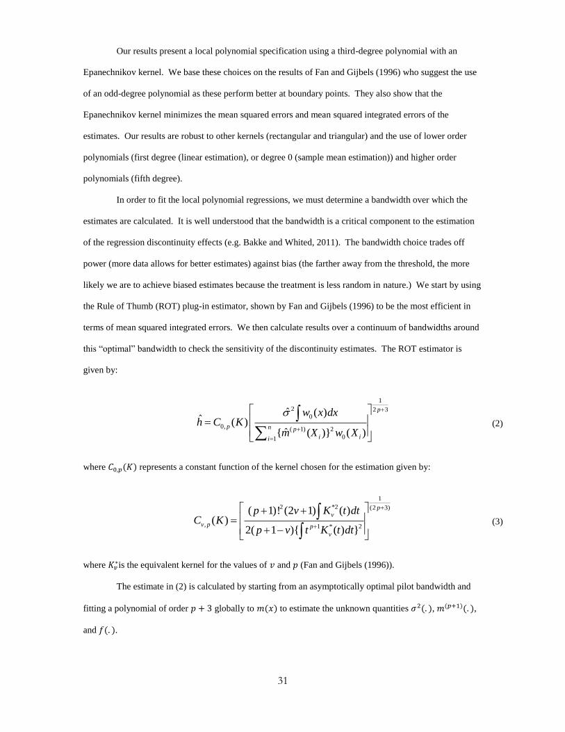
Our results present a local polynomial specification using a third-degree polynomial with an

Epanechnikov kernel. We base these choices on the results of Fan and Gijbels (1996) who suggest the use

of an odd-degree polynomial as these perform better at boundary points. They also show that the

Epanechnikov kernel minimizes the mean squared errors and mean squared integrated errors of the

estimates. Our results are robust to other kernels (rectangular and triangular) and the use of lower order

polynomials (first degree (linear estimation), or degree 0 (sample mean estimation)) and higher order

polynomials (fifth degree).

In order to fit the local polynomial regressions, we must determine a bandwidth over which the

estimates are calculated. It is well understood that the bandwidth is a critical component to the estimation

of the regression discontinuity effects (e.g. Bakke and Whited, 2011). The bandwidth choice trades off

power (more data allows for better estimates) against bias (the farther away from the threshold, the more

likely we are to achieve biased estimates because the treatment is less random in nature.) We start by using

the Rule of Thumb (ROT) plug-in estimator, shown by Fan and Gijbels (1996) to be the most efficient in

terms of mean squared integrated errors. We then calculate results over a continuum of bandwidths around

this “optimal” bandwidth to check the sensitivity of the discontinuity estimates. The ROT estimator is

given by:

(2)

where represents a constant function of the kernel chosen for the estimation given by:

(3)

where is the equivalent kernel for the values of and (Fan and Gijbels (1996)).

The estimate in (2) is calculated by starting from an asymptotically optimal pilot bandwidth and

fitting a polynomial of order globally to to estimate the unknown quantities , ,

and .

1

2 2 30

0, ( 1) 2

01

ˆ ( )ˆ ( )

ˆ{ ( )} ( )

p

p n p

i ii

w x dxh C K

m X w X

1

2 *2 (2 3)

, 1 * 2

( 1)! (2 1) ( )( )

2( 1 ){ ( ) }

pv

v p p

v

p v K t dtC K

p v t K t dt

32

The shape of the data to the left of the threshold may differ substantially from the data to the right.

As a result, we may have very different optimal bandwidths to the right and left. In examining the

sensitivity of estimates for smaller and larger bandwidths, we do so proportionally to the original ROT

bandwidth estimates.

After choosing the optimal bandwidth, we estimate the local polynomial regressions to the left and

the right of the threshold. We then measure the distance between these two estimates at the threshold point.

In order to test the difference between these two estimates, we bootstrap the standard errors, sampling with

replacement from the data, and impose a restriction that ensures sampling from each decile of ranks in the

Russell 3000 (to ensure some data around the threshold). These results are robust to an unrestricted

bootstrap sample.

To further demonstrate the significance of the threshold effect we report, we use a falsification

exercise in which we use the above estimation technique over a large number of randomly selected placebo

thresholds and report the distribution of measured discontinuities. These results demonstrate that not only

is the effect statistically significant at the true threshold, it is larger than the effects measured at random

thresholds. This provides for a robustness check in case the methodology over rejects the null at any

threshold by comparing the magnitudes of the estimates at the true threshold against the estimates over

1,000 placebo threshold tests (see section III for further discussion.)

Valid causal identification of the regression discontinuity design relies on the randomness of the

allocation around the threshold. This assumption can be tested empirically by looking at firms’

characteristics in the year prior to the treatment, and ensuring that these firms are similar around the

threshold. We discuss issues related to randomness in section I.C.

The randomness argument is also key to understanding why the study of “switchers”, firms that

move from one index to the other, is not helpful in identifying a causal treatment effect in our case. When

looking at all "switchers" the causal inference is invalidated by the fact these firms changed index for a

reason that may be related to the corporate policy of interest (e.g. firms may increase dividend payment if

they become smaller and move from the Russell 1000 index to the Russell 2000 index because their

investment opportunities shrink.) To avoid this selection issue, we would need to restrict ourselves to firms

that have moved from one index to the other with only minor changes in their relative market capitalization

ranking. In our case this would require that firms be on different sides of the threshold in consecutive years

33

but be within a small bandwidth of the threshold in both. This constraint severely restricts the size of the

sample over which we can base our inference. We only find around 10 switchers each year on either side

of a 100 rank bandwidth. Like most regression discontinuity design studies, we do not look at switchers in

this paper for this reason.

34

Appendix 2 Definition of Main Variables

Book Leverage Compustat Total Debt (DLC + DLTT) scaled by total assets (AT)

Cash Holdings Cash and Short Term Investments (CHE) scaled by total assets (AT)

Institutional Ownership Thomson 13F Shares Held summed across all institutions scaled by CRSP shares

outstanding (SHROUT)

Ln (Cash Holdings) Ln (Cash and Short Term Investment (CHE))

Ln (Dividends) Ln (Compustat Dividends (DVC+DVP))

Ln (Net Equity Issuance) Ln (Sale of Common and Preferred Shares (SSTK) -Share Repurchases (PRSTKC))

Ln (Net Financing) Ln (Net Equity Issuance+Change in Total Debt [(DD1+DLTT)-(DD1+DLTT)t-1])

Ln (Repurchases) Ln(Purchase of Common and Preferred Shares (PRSTKC))

Ln(R&D Expense) Ln(Research and Development Expenses (XRD))

Ln (Total Payout) Ln (Compustat Dividends (DVC+DVP) plus Purchase of Common and Preferred

Shares (PRSTKC))

Market-to-Book ratio Market value of equity (PRCC x CSHPRI) plus total debt (DLC+DLTT) plus

preferred stock (PSTKL) minus deferred taxes, all scaled by book value of total assets

(AT).

Market Leverage Compustat Total Debt (DLC + DLTT) scaled by Market value of equity (PRCC x

CSHPRI)

Market Value CRSP Price (PRC) multiplied by shares outstanding (SHROUT)

ROA Operating Income Before Depreciation (OIBDP) scaled by lagged total assets (AT)

35

Figure 1 - Russell Index Weights Around the Threshold

This figure shows the average index weights for firms in the Russell 1000 and firms in the Russell 2000. Firms are

assigned to the Russell 1000 or 2000 based on the market cap of the firm at the end of May each year. Index

weights are determined by using a float adjusted market cap within each index at the end of June.

36

Figure 2 – Institutional Ownership Discontinuity Panel A, B, C, and D show the Total Institutional Ownership for the first quarter ending after the reconstitution of the Russell indices for the

Russell 3000 firms from 1991-2008. The X axis represents the distance from the Russell 1000/2000 threshold, with 0 representing the last firm in the Russell 1000. Panel A plots the average Total Institutional Ownership over 10 ranks across all years. Panel B adds local polynomial

regression estimates and the associated 90% confidence bands using the Rule of Thumb (ROT) optimal plug-in bandwidth estimate of Fan and

Gijbels (1996). Panel E shows the estimate of the Total Institutional Ownership discontinuity for the same period. The X axis represents the size of the bandwidth used in the estimation as a percentage of the optimal ROT bandwidth, with 0 representing the estimate at the ROT choice. The

solid line is the point estimate of the discontinuity and the dashed line represent the 90% confidence bands from bootstrapped standard errors.

Panel F shows estimates of the Total Institutional Ownership discontinuity for simulations of 1000 random placebo thresholds. The vertical dashed line represents the estimate at the true threshold.

37

Figure 3 – Dividends Discontinuity Panel A, B, C, and D show the Ln(Dividend) for the first fiscal year ending at least 12 months after the reconstitution of the Russell indices for

the Russell 3000 firms from 1991-2008. The X axis represents the distance from the Russell 1000/2000 threshold, with 0 representing the last firm in the Russell 1000. Panel A plots the average Ln(Dividend) over 10 ranks across all years. Panel B adds local polynomial regression

estimates and the associated 90% confidence bands using the Rule of Thumb (ROT) optimal plug-in bandwidth estimate of Fan and Gijbels

(1996). Panel E shows the estimate of the Ln(Dividend) discontinuity for the same period. The X axis represents the size of the bandwidth used in the estimation as a percentage of the optimal ROT bandwidth, with 0 representing the estimate at the ROT choice. The solid line is the point

estimate of the discontinuity and the dashed line represent the 90% confidence bands from bootstrapped standard errors. Panel F shows estimates

of the Ln(Dividend) discontinuity for simulations of 1000 random placebo thresholds. The vertical dashed line represents the estimate at the true threshold.

38

Figure 4 – Total Payout Discontinuity

Panel A, B, C, and D show the Ln(Total Payout) for the first fiscal year ending at least 12 months after the reconstitution of the Russell indices for the Russell

3000 firms from 1991-2008. The X axis represents the distance from the Russell 1000/2000 threshold, with 0 representing the last firm in the Russell 1000.

Panel A plots the average Ln(Total Payout) over 10 ranks across all years. Panel B adds local polynomial regression estimates and the associated 90% confidence bands using the Rule of Thumb (ROT) optimal plug-in bandwidth estimate of Fan and Gijbels (1996). Panel E shows the estimate of the Ln(Total

Payout) discontinuity for the same period. The X axis represents the size of the bandwidth used in the estimation as a percentage of the optimal ROT

bandwidth, with 0 representing the estimate at the ROT choice. The solid line is the point estimate of the discontinuity and the dashed line represent the 90% confidence bands from bootstrapped standard errors. Panel F shows estimates of the Ln(Total Payout) discontinuity for simulations of 1000 random placebo

thresholds. The vertical dashed line represents the estimate at the true threshold.

39

Figure 5 – Cash Holdings Discontinuity

Panel A, B, C, and D show the Ln (Cash Holdings) for the first fiscal year ending at least 12 months after the reconstitution of the Russell indices for the Russell 3000 firms from 1991-2008. The X axis represents the distance from the Russell 1000/2000 threshold, with 0 representing the last

firm in the Russell 1000. Panel A plots the average in Ln (Cash Holdings) over 10 ranks across all years. Panel B adds local polynomial

regression estimates and the associated 90% confidence bands using the Rule of Thumb (ROT) optimal plug-in bandwidth estimate of Fan and Gijbels (1996). Panel E shows the estimate of the Ln (Cash Holdings) discontinuity for the same period. The X axis represents the size of the

bandwidth used in the estimation as a percentage of the optimal ROT bandwidth, with 0 representing the estimate at the ROT choice. The solid

line is the point estimate of the discontinuity and the dashed line represent the 90% confidence bands from bootstrapped standard errors. Panel F shows estimates of the Ln (Cash Holdings) discontinuity for simulations of 1000 random placebo thresholds. The vertical dashed line represents

the estimate at the true threshold.

40

Figure 6 – Proxy-voting Participation Panel A, B, C, and D show the proxy-voting participation for the first fiscal year ending at least 12 months after the reconstitution of the Russell

indices for the Russell 3000 firms from 1991-2008. The X axis represents the distance from the Russell 1000/2000 threshold, with 0 representing the last firm in the Russell 1000. Panel A plots the average change in Ln (Voting Percentage/(1-Voting Percentage)) over 10 ranks across all

years. Panel B adds local polynomial regression estimates and the associated 90% confidence bands using the Rule of Thumb (ROT) optimal

plug-in bandwidth estimate of Fan and Gijbels (1996). Panel E shows the estimate of the voting participation discontinuity for the same period. The X axis represents the size of the bandwidth used in the estimation as a percentage of the optimal ROT bandwidth, with 0 representing the

estimate at the ROT choice. The solid line is the point estimate of the discontinuity and the dashed line represent the 90% confidence bands from

bootstrapped standard errors. Panel F shows estimates of the voting participation discontinuity for simulations of 1000 random placebo thresholds. The vertical dashed line represents the estimate at the true threshold.

41

Table I – Summary Statistics These tables present the summary statistics for firms that belong to the Russell 1000 index (Panel A) and to the Russell 2000

index (Panel B). Variables are defined in the Appendix 2.

Panel A: Russell 1000 Mean StdDev p25 Median p75

Institutional Ownership 0.65 0.22 0.50 0.67 0.81

ROA 0.16 0.12 0.08 0.14 0.21

Dividend Yield 0.02 0.02 0.00 0.01 0.03

Book Leverage 0.25 0.19 0.10 0.24 0.37

Payout/Assets 0.05 0.06 0.01 0.02 0.06

Repurchases/Assets 0.03 0.05 0.00 0.00 0.03

Cash/Assets 0.14 0.21 0.02 0.06 0.17

Total Assets (B$ 2005) 1.06 1.61 0.15 0.39 1.12

Market Value (B$ 2005) 7.29 11.40 1.55 3.00 6.99

Cash Holdings (M$ 2005) 798 1,409 58 218 753

Payout (M$ 2005) 284 475 17 89 285

Repurchases (M$ 2005) 148 295 0.00 9.64 129

Dividends (M$ 2005) 119 201 0.00 34.59 127

Panel B: Russell 2000 Mean StdDev p25 Median p75

Institutional Ownership 0.52 0.28 0.28 0.50 0.73

ROA 0.10 0.19 0.03 0.11 0.19

Dividend Yield 0.01 0.02 0.00 0.00 0.02

Book Leverage 0.22 0.22 0.02 0.17 0.35

Payout/Assets 0.03 0.05 0.00 0.01 0.03

Repurchases/Assets 0.01 0.04 0.00 0.00 0.01

Cash/Assets 0.22 0.30 0.03 0.09 0.29

Total Assets (B$ 2005) 0.97 1.94 0.16 0.39 1.02

Market Value (B$ 2005) 0.46 0.41 0.177 0.320 0.607

Cash Holdings (M$ 2005) 83 182 10.17 34.4 92

Payout (M$ 2005) 15.20 41 0.00 2.19 14

Repurchases (M$ 2005) 7.83 28 0.00 0.00 2.65

Dividends (M$ 2005) 7.42 24 0.00 0.00 6.21

42

Table II - Pre-treatment Sample Differences

at the Russell 1000/2000 Threshold

This table presents the local polynomial values at the Russell 1000/2000 threshold of the dependent variables in the year prior

to the index assignment. Regression discontinuity test results are presented, where τ is estimated by fitting a third degree

polynomial estimate to the left and to the right within the given bandwidth. We report estimates of τ and the bootstrapped z-

stats. Variables are defined in detailed in Appendix 2. Superscript a, b, and c indicate a significance level of less than 10%, 5%,

and 1% respectively.

Variable

Just

Included

(Left)

Just

Excluded

(Right)

Treatment

(τ)

z-stat

ROT Bandwidth

Institutional Ownershipt+1 0.66 0.65 -0.01 -0.1 73 184

Ln(Market Value)t-1 14.17 14.04 -0.03 -1.05 78 188

Annual Returnt-1 0.22 0.20 -0.02 -0.19 121 177

ROAt-1 0.12 0.14 0.02 1.09 92 254

Market to Bookt-1 1.58 1.77 0.19 0.79 90 242

Market Leveraget-1 0.32 0.28 -0.05 -1.24 94 146

Ln(Dividends)t-1 1.90 1.87 -0.03 -0.1 72 288

Ln(Total Payout)t-1 2.67 2.64 -0.11 -0.11 87 176

Ln(Repurchases)t-1 1.30 1.35 0.05 0.18 91 189

Ln(Net Equity Issuance)t-1 2.19 2.19 0.02 0.02 101 222

Ln(Net Financing)t-1 -3.64 -2.77 0.04 1.32 85 192

Ln(Cash Holdings)t-1 4.37 4.13 -0.24 -1.36 85 215

43

Table III– Discontinuity Statistics for Payout Policy This table presents the regression discontinuity test results where τ is estimated by fitting a third degree polynomial estimate to

the left and to the right of the Russell 1000/2000 threshold. We report estimates of τ and the z-stats in parentheses. Variables are

defined in detailed in Appendix 2. Superscript a, b, and c indicate a significance level of less than 10%, 5%, and 1%

respectively.

Dependent Variable Treatment (τ) ROT Bandwidth

Institutional Ownershipt+1 9.18% 70 190

(2.15)b

Ln(Dividends)t+1 0.73M 86 245

(2.25)b

Ln(Total Payout)t+1 0.75M 110 181

(2.31)b

Ln(Repurchases)t+1 0.93M 97 213

(2.22)b

44

Table IV– Cross-Sectional Results:

The Effects of Ex-Ante Agency Costs This table presents the regression discontinuity test results where τ is estimated by fitting a third degree polynomial

estimate to the left and to the right of the Russell 1000/2000 threshold. We report estimates of τ and the t-stats in

parentheses separately for High ROA firms (firms with ROA above the median), low ROA firms (firms with ROA

below the median), high growth option firms (market to book above median) and low growth option firms (market

to book below median), high and low free cash flow (high cash flow and low growth opportunities vs. low cash flow

and high growth opportunities), high and low total compensation (total direct compensation per Execucomp), and

high and low analyst coverage (number of analysts above and below median.) Variables are defined in detailed in

Appendix 2. Superscript a, b, and c indicate a significance level of less than 10%, 5%, and 1% respectively.

Treatment effects for Total Payout

ROA

Market-to-

book

Cash/

Investment

Total Comp.

Analyst

Coverage

High group treatment effect -0.44 0.001 1.16 1.51 0.3

(1.29) (0.00) (2.38)a

(2.14)b

(0.62)

Low group treatment effect 0.55 0.53 0.45 -1.05 -0.51

(1.53) (1.87)c

(1.13) (-1.63) (-1.41)

Difference (High-Low) -0.99 -0.53 0.72 2.56 0.81

(-1.66)c (-1.14) -1.48 (2.15)

b (1.39)

45

Table V– Discontinuity Statistics for Other Corporate Policies This table presents the regression discontinuity test results where τ is estimated by fitting a third degree polynomial estimate to

the left and to the right of the Russell 1000/2000 threshold. We report estimates of τ and the z-stats in parentheses. Variables are

defined in detailed in Appendix 2. Superscript a, b, and c indicate a significance level of less than 10%, 5%, and 1%

respectively.

Dependent Variable Treatment (τ) ROT Bandwidth

Ln(Cash Holdings)t+1 -0.32M 78 210

(-1.68)c

Ln(Net Equity Issuance)t+1 1.08M 122 185

(2.52)a

Asset Growth 0.34 97 176

(4.91)a

Ln(R&D Expense) t+1 0.48M 91 164

(1.78)c