Embed Size (px)
Citation preview
NBP Working Paper No. 289
The effect of house prices on bank risk: empirical evidence from Hungary
Ádám Banai, Nikolett Vágó

Economic Research DepartmentWarsaw 2018
NBP Working Paper No. 289
The effect of house prices on bank risk: empirical evidence from Hungary
Ádám Banai, Nikolett Vágó

Published by: Narodowy Bank Polski Education & Publishing Department ul. Świętokrzyska 11/21 00-919 Warszawa, Poland www.nbp.pl
ISSN 2084-624X
© Copyright Narodowy Bank Polski 2018
Ádám Banai – Magyar Nemzeti Bank; [email protected] Vágó – Magyar Nemzeti Bank; [email protected]
Disclaimer:The views expressed in this paper are those of the authors and do not necessarily reflect the official view of the Magyar Nemzeti Bank.
Acknowledgements:The authors would like to thank Bálint Dancsik and Mikko Mäkinen for their valuable suggestions. They are also grateful for the participants of the “Recent trends in the real estate market and its analysis (2017)” workshop in Warsaw, and the “15th ESCB Emerging Markets (2017)” workshop in Saariselka for their useful comments.

3NBP Working Paper No. 289
ContentsAbstract 41. Introduction 52. Data 83. Methodology 114. Results 135. Robustness tests 196. Conclusion 22References 24Appendix 26
Narodowy Bank Polski4
Abstract
2
Abstract
Housing market is important from a macroprudential perspective because it has a strong effect
on the banking sector. Changes in real estate prices may affect the level of bank risk through
household mortgage lending, however, the literature has no clear conclusion on this impact
mechanism. Using a bank-level database containing quarterly data from 1998 to 2016 we
estimated dynamic fixed-effects panel models to examine how bank risk is influenced by
housing prices via mortgage lending in the Hungarian banking system. According to the
results (1) higher house prices lead to higher bank risk, (2) the higher the share of mortgage
loans at a bank, the stronger the positive effect of house prices on bank risk. In the period
following the onset of the crisis a much stronger positive relationship could be observed
between house prices and bank risk than before the crisis. Using the house price gap which
measures the deviation of house prices from their fundamental value we provide empirical
evidence that the deviation hypothesis was stronger for Hungary. This suggests that both
banks and households tend to undertake excessive risks during a housing market boom, which
can be mitigated by macroprudential policy instruments.
Keywords: bank risk, house price index, mortgage loan, real estate market
JEL Codes: G21;G28; G30; C23

5NBP Working Paper No. 289
Chapter 1
3
1. Introduction
Housing market has a strong effect on the economy as a whole. As residential property is the
main asset of Hungarian households, consumption and saving decisions are strongly
influenced by house prices. In the corporate sector, property prices and number of transactions
influences demand for new investments, and ultimately has an effect on the construction
industry and its suppliers.
This strong effect also appears in the banking sector. The performance of mortgage loans,
which account for a major portion of household loans, is determined by the property market
in several respects. A decline in house prices causes banks’ expected loan losses to increase
for two reasons: (1) the value of collateral decreases, which raises the loss given default
(LGD); and (2) the probability of default (PD) increases as it becomes less worthwhile for the
borrower to continue servicing the debt. In the corporate sector, a decline in property prices
may have a negative effect through the construction industry in particular, because it lowers
the number of investments and the profitability of construction firms, which ultimately also
has a negative effect on the performance of bank exposures related to the real estate sector.
These factors affect both capital position and P&L through impairment, eroding the stability
of financial institutions. Conversely, when property prices rise, the exact opposite may occur,
strengthening banks’ positions. Moreover, rising real estate prices support the launch of new
investments and lead to stronger bank activity, which, inter alia, can improve profitability
and help to maintain a low NPL ratio, i.e. reinforce institutional stability.
Apart from the obvious impact mechanisms mentioned above, rising property prices can also
increase risks. Higher house prices make property purchases more attractive, while also
motivating banks to lend more actively. One possible result can be that the banking sector
serves increasingly poor quality borrowers by selling increasingly risky loan products, as
shown by the example of the US subprime market. It should be noted that foreign currency
lending in Hungary also exhibited these features in 2007–2008 (Balás et al., 2015).
Additionally, with a rapid rise in house prices, banks which are active in mortgage lending
become more exposed to a potential downturn in the property market, possibly posing a major
risk to bank stability, particularly when this is associated with high indebtedness among
borrowers.
Our study identifies the effect of house prices on bank stability and examines whether the size
of the effect depends on banks’ exposures to the housing market. This question is highly
relevant in terms of policy, as the macroprudential toolkit includes several instruments that

Narodowy Bank Polski6
4
can be used to mitigate risks related to the real estate market. For example, implementation
of sector-specific macroprudential rules (i.e. higher risk weights or minimum LGD values for
portfolios with real estate collateral; ESRB 2016) may help to mitigate the vulnerability of
the banking sector, when risks of banks with larger housing market exposures increase at a
relatively faster rate than the increase in house prices.1
Analyses of the effect of house prices on bank risks have the same dual nature as described
above. Studies report varying results on the interaction of house prices – or more broadly,
mortgage lending – and risks. Although Blasko and Sinkey’s (2006) study of the US banking
sector was not directly focused on house prices, its findings on the interaction between
intensifying mortgage lending and bank risks are relevant for us. The authors analysed the
entire banking sector over the period between 1989 and 1996 and found that regulations
increasingly pushed banks towards mortgage lending, because that was considered to be the
least risky. As a result, however, banks which engaged more actively in mortgage lending
became relatively risky. By contrast, less specialised institutions demonstrated better stability
in the period under review. However, that finding does not necessarily derive from the higher
risk of mortgage loans; it is possible that the relative safety of mortgage loans encourages
banks to take more risk. Koetter and Poghosyan (2010) specifically examined the direct effect
of house prices on bank risk. The authors tested two hypotheses on the relation between the
German banking sector and the real estate markets of various regions. Their results failed to
confirm the collateral value hypothesis, i.e. rising house prices reduce bank risks due to more
favourable LGD and PD levels. Conversely, they showed that the deviation hypothesis could
be accepted, i.e. that deviation from the equilibrium value increased bank risks. Somewhat in
contrast to these findings, Gibilaro and Mattarocci (2016) examined a broader international
sample and demonstrated a clearly positive correlation between house price levels and bank
stability, as measured by the Z-risk indicator. They found that rising house prices improved
banks’ profitability and capital position. Importantly, however, the authors found that this
positive effect only applied to banks which were not specialised in household mortgage
lending. With banks engaged in mortgage lending, no causal relationship could be shown
between house prices and Z-risk, because that risk is probably better managed by specialised
institutions. Following the approach of Gibilaro and Mattarocci (2013), Rebi (2016)
1 Restrictions on the loan-to-value, loan-to-income and payment-to-income (LTV, LTI and PTI) indicators, which are now used quite widely, affect banks’ new lending. Therefore, such restrictions are mainly suitable to alleviate the further accumulation of risks rather than to mitigate risks from existing exposures.
5
performed a similar analysis of the Albanian banking sector and found that banks with higher
mortgage loan ratios seem to be riskier through their relatively larger exposure to housing
market developments. Empirical results show that rising house prices mitigate the risk of so-
called “non-real estate” banks (which had a ratio of mortgage loans of less than 20 per cent in
five consecutive years), while leading to higher riskiness in the case of “real-estate” banks.
Literature shows considerable variations in terms of methodology, and conclusions also differ
occasionally. Koetter and Poghosyan (2010) underline that the results may depend strongly
on the housing market on which the hypotheses are tested, given that e.g. imbalances were
significantly more limited in the German housing market compared to the US or Spanish
markets.
Several key issues arise based on the literature with a potentially significant effect on results.
In our paper we investigate the relationship of bank risk and real estate prices with strict focus
on essential issues suggested by the existing literature. (1) A fundamental question suggested
by Gibilaro and Mattarocci (2016) is whether the institution concerned is specialised or not,
for which we control in our analysis. (2) Koetter and Poghosyan (2010) demonstrated that the
level of house prices and deviation of house prices from the equilibrium may produce different
effects. In our study, we consider both approaches in order to develop a better understanding
of the effect of the real estate market. (3) We find that the method of measuring risk is also
relevant. While studies generally use the Z-risk indicator (Rebi 2016, Blasko and Sinkey
2006, Gibilaro and Mattarocci 2016) as dependent variable, Koetter and Poghosyan (2010)
measure bank risk with a probability of bank default indicator. In our research, we also test
the influence of the risk indicator on the result, i.e. the extent to which the effect measured
depends on the definition of bank risk.
It should also be pointed out that most studies examine the household and corporate sectors
jointly. We do not consider this expedient for two reasons. First, lending is often significantly
different in the household and corporate sectors: for example, in Hungary before the onset of
the crisis, the estimated size of the credit gap in the market for household loans was 1.5 times
that of the corporate market (Hosszú et al., 2014). Second, there may be significant difference
in the risk of the residential and commercial property markets. Developments in the housing
and commercial property markets may affect bank stability in different ways. As our research
is focused exclusively on the housing market, we use a house price index to capture
developments in the real estate market, while using banks’ exposure to the household
mortgage loan market to measure their relationship with the property market.
6
Section 2 of the paper describes the data used, while Section 3 set out the methodology
applied. The results are presented in Section 4. A detailed robustness test is performed in
Section 5. A conclusion based on our findings is provided in Section 6.

7NBP Working Paper No. 289
Introduction
5
performed a similar analysis of the Albanian banking sector and found that banks with higher
mortgage loan ratios seem to be riskier through their relatively larger exposure to housing
market developments. Empirical results show that rising house prices mitigate the risk of so-
called “non-real estate” banks (which had a ratio of mortgage loans of less than 20 per cent in
five consecutive years), while leading to higher riskiness in the case of “real-estate” banks.
Literature shows considerable variations in terms of methodology, and conclusions also differ
occasionally. Koetter and Poghosyan (2010) underline that the results may depend strongly
on the housing market on which the hypotheses are tested, given that e.g. imbalances were
significantly more limited in the German housing market compared to the US or Spanish
markets.
Several key issues arise based on the literature with a potentially significant effect on results.
In our paper we investigate the relationship of bank risk and real estate prices with strict focus
on essential issues suggested by the existing literature. (1) A fundamental question suggested
by Gibilaro and Mattarocci (2016) is whether the institution concerned is specialised or not,
for which we control in our analysis. (2) Koetter and Poghosyan (2010) demonstrated that the
level of house prices and deviation of house prices from the equilibrium may produce different
effects. In our study, we consider both approaches in order to develop a better understanding
of the effect of the real estate market. (3) We find that the method of measuring risk is also
relevant. While studies generally use the Z-risk indicator (Rebi 2016, Blasko and Sinkey
2006, Gibilaro and Mattarocci 2016) as dependent variable, Koetter and Poghosyan (2010)
measure bank risk with a probability of bank default indicator. In our research, we also test
the influence of the risk indicator on the result, i.e. the extent to which the effect measured
depends on the definition of bank risk.
It should also be pointed out that most studies examine the household and corporate sectors
jointly. We do not consider this expedient for two reasons. First, lending is often significantly
different in the household and corporate sectors: for example, in Hungary before the onset of
the crisis, the estimated size of the credit gap in the market for household loans was 1.5 times
that of the corporate market (Hosszú et al., 2014). Second, there may be significant difference
in the risk of the residential and commercial property markets. Developments in the housing
and commercial property markets may affect bank stability in different ways. As our research
is focused exclusively on the housing market, we use a house price index to capture
developments in the real estate market, while using banks’ exposure to the household
mortgage loan market to measure their relationship with the property market.
6
Section 2 of the paper describes the data used, while Section 3 set out the methodology
applied. The results are presented in Section 4. A detailed robustness test is performed in
Section 5. A conclusion based on our findings is provided in Section 6.

Narodowy Bank Polski8
Chapter 2
7
2. Data
In our study, we used a unique bank-level database containing Hungarian banks present in the
Hungarian banking market since late 1998, which were active in mortgage lending (i.e. the
observation period included sections where the bank concerned reached a market share of at
least 1 per cent). Ultimately, 13 banks were included in the sample, which contains quarterly
data from 1998 Q4 to 2016 Q2. Specific bank characteristics were merged with
macroeconomic variables, also measured on a quarterly basis. The descriptive statistics on the
variables presented in the following are included in Table 5 in the Annex.
Our dependent variable is a bank risk indicator which is compiled closely following the
approach used by the EBA (EBA 2015) for deposit guarantee purposes.2 The risk indicator
contains six bank characteristics (Table 1), each assigned a risk rating between 0 and 100
based on thresholds defined for the Hungarian market, with higher values indicating higher
bank risk. The bank risk indicator used as the dependent variable in our models is generated
by aggregating the six risk indicators using the proportionately rescaled weights of the EBA
guideline.
Although different types of Z-risk measures are commonly used in the literature as risk
indicators, we decided to use this composite indicator containing information on several
aspects of riskiness. While Z-risk focuses only on leverage and profitability, our measure has
a broader perspective. As suggested by experiences from the global financial crisis (GFC),
capital adequacy and asset quality are also important, considering the impact of a housing
boom on liquidity. As Blasko and Sinkey (2006) suggested, a rise in house prices increases
the risk-taking of banks. But this phenomenon is not necessarily reflected by the leverage.
Moreover, taking a medium-term horizon this higher risk-taking may improve profitability
with relatively stable leverage, but the riskiness of mortgages (e.g. high PTI, high LTV
contracts, subprime borrowers, etc.) increases, as reflected by the capital adequacy. The kind
of composite indicator we use provides a clearer picture of the riskiness of banks by
containing information on riskiness from several different perspectives.
2 We modified the methodology proposed by the EBA in that we: (1) disregarded covered deposits for the calculation of the risk indicator which is only important for deposit insurance agencies, (2) included one liquidity indicator instead of LCR and NSFR ratios and proportionately modified the original weights. Precise LCR and NSFR data are not available for such a long observation period.

9NBP Working Paper No. 289
Data
7
2. Data
In our study, we used a unique bank-level database containing Hungarian banks present in the
Hungarian banking market since late 1998, which were active in mortgage lending (i.e. the
observation period included sections where the bank concerned reached a market share of at
least 1 per cent). Ultimately, 13 banks were included in the sample, which contains quarterly
data from 1998 Q4 to 2016 Q2. Specific bank characteristics were merged with
macroeconomic variables, also measured on a quarterly basis. The descriptive statistics on the
variables presented in the following are included in Table 5 in the Annex.
Our dependent variable is a bank risk indicator which is compiled closely following the
approach used by the EBA (EBA 2015) for deposit guarantee purposes.2 The risk indicator
contains six bank characteristics (Table 1), each assigned a risk rating between 0 and 100
based on thresholds defined for the Hungarian market, with higher values indicating higher
bank risk. The bank risk indicator used as the dependent variable in our models is generated
by aggregating the six risk indicators using the proportionately rescaled weights of the EBA
guideline.
Although different types of Z-risk measures are commonly used in the literature as risk
indicators, we decided to use this composite indicator containing information on several
aspects of riskiness. While Z-risk focuses only on leverage and profitability, our measure has
a broader perspective. As suggested by experiences from the global financial crisis (GFC),
capital adequacy and asset quality are also important, considering the impact of a housing
boom on liquidity. As Blasko and Sinkey (2006) suggested, a rise in house prices increases
the risk-taking of banks. But this phenomenon is not necessarily reflected by the leverage.
Moreover, taking a medium-term horizon this higher risk-taking may improve profitability
with relatively stable leverage, but the riskiness of mortgages (e.g. high PTI, high LTV
contracts, subprime borrowers, etc.) increases, as reflected by the capital adequacy. The kind
of composite indicator we use provides a clearer picture of the riskiness of banks by
containing information on riskiness from several different perspectives.
2 We modified the methodology proposed by the EBA in that we: (1) disregarded covered deposits for the calculation of the risk indicator which is only important for deposit insurance agencies, (2) included one liquidity indicator instead of LCR and NSFR ratios and proportionately modified the original weights. Precise LCR and NSFR data are not available for such a long observation period.
8
Table 1: Components of the bank risk indicator
Bank characteristic Variable Definition Weight Capital Leverage ratio Regulatory capital / Total assets 14%
Capital adequacy ratio
Regulatory capital / Risk-weighted assets 14%
Liquidity Liquidity ratio Liquid assets / Total assets 29%
Asset quality Non-performing loans ratio
Non-performing loans / Total loans 22%
Business model, management
Riskiness of assets Risk-weighted assets / Total assets 10%
Return on assets Average Net income / Total assets 10%
To compare, we also estimate models with the Z-risk indicator, as it is applied broadly in the
literature. The Z-risk indicator proposed by Lepetit et al. (2013) is calculated in the following
manner:
where is the mean, while is the standard deviation of the return on assets, both calculated over the full sample; and is the ratio of equity capital to total assets.
The significance of banks’ activity on the mortgage loan market was tested in two ways. On
the one hand, we used the share of mortgage loans within total loans as a continuous variable
(‘Mortgage Ratio’), and on the other hand, a dummy variable was created, which takes the
value of 1 for banks that are active in the mortgage loan market, i.e. mortgage loans represent
at least 30% of their total loans (‘Mortgage Ratio>30%’). Figure 6 in the Annex provides
insight on the dynamics and distribution of banks’ mortgage lending ratio in the Hungarian
banking system.
The most important macro variable in the model is the house price index (‘HPI’), which is
the main focus of our research. This variable was measured by the MNB real house price
index (Figure 5 in the Annex). For robustness tests, we also used the house price gap
(‘HPG’),3 which is the deviation of house prices from the level justified by fundamentals. As
a macro-level control variable, for specific estimates we also used the annual growth rates of
3 The house price gap is the average of the gaps derived as the difference between the MNB real house price index and the equilibrium house price levels obtained from various estimates (MNB, 2017, p.12).

Narodowy Bank Polski10
9
GDP (‘GDP (agr)’), real disposable income (‘Disp. Income (agr)’) and the short-term interest
rate (3-month BUBOR, ‘Interest Rate (agr)’).
As bank-level control variables, the models included the capital adequacy ratio (‘CAR’), the
ratio of liquid assets to total assets (‘Liquid assets ratio’), the ratio of non-performing loans
(‘NPL’), the return on total assets (‘ROA’) and the share of foreign funds within the balance
sheet (‘Foreign funds ratio’).

11NBP Working Paper No. 289
Chapter 3
9
GDP (‘GDP (agr)’), real disposable income (‘Disp. Income (agr)’) and the short-term interest
rate (3-month BUBOR, ‘Interest Rate (agr)’).
As bank-level control variables, the models included the capital adequacy ratio (‘CAR’), the
ratio of liquid assets to total assets (‘Liquid assets ratio’), the ratio of non-performing loans
(‘NPL’), the return on total assets (‘ROA’) and the share of foreign funds within the balance
sheet (‘Foreign funds ratio’).
10
3. Methodology
We examined the effect of the house prices and mortgage exposure on bank stability in the
following dynamic fixed-effects panel model:
��� � � ������ � �������� � φ� ��� � �� � �� � ���
for i=1, …, N and t=1, …, T. ��� is the dependent variable, ������ is the lagged dependent
variable, ������ is the vector of the independent variables in our focus4 (housing market
exposure, house price index, and the interaction thereof), ��� is the vector of bank
characteristics included as control variables, � is the coefficient of the lag, while � and φ are
vectors of the coefficients relating to independent variables. �� is the cross-sectional fixed
effect, �� is the period fixed effect, ��� is the idiosyncratic error term with ������=0,
���������= ��� if j=i and t=s, otherwise ���������= 0.
We opted for fixed-effect panel regression as we assume that developments in the dependent
variable are unobservable and vary by bank.5 The fixed-effect component (��) used in the
model controls for unobserved heterogeneity across banks that is constant over time. As the
time-series dimension of our panel is long (66 quarters) and much larger than the cross-
sectional dimension (13 banks), we used the within regression estimator. Driscoll–Kraay
(1998) standard errors were calculated,6 which are robust in terms of heteroskedasticity,
higher orders of autocorrelation and cross-sectional dependence (Hoeche, 2007).
Including the lagged dependent variable as an independent variable can result in biased
estimates if the time dimension of the database is small (Nickell, 1981).7 As T=30 is a border-
4 The quarterly lags of these variables are included in the model, as we doubt that their effect would appear simultaneously in the risk indicator. For example, although the GFC significantly changed the state of banks, it took several quarters before the negative effect was reflected by risk indicators.
5 The assumption of the fixed effects method (FE) is that the unobserved variable and the independent variables are correlated. The null hypothesis on no correlation between the unobserved variable and independent variables is rejected on the basis of the Hausman test. Consequently, the estimation of the random effects model (RE) is inconsistent and biased, which confirms the selection of the FE method.
6 We examined whether the usual assumptions of the FE method were satisfied. We carried out formal tests to determine whether (1) the error term of the model is homoscedastic, (2) the error terms are autocorrelated up to some lag, and (3) cross-sectional dependence is present in the database. Based on test results, the error terms are heteroscedastic and autocorrelated, but cross-sectional dependence is not present in the data. 7 Nickell proved analytically that in case of dynamic panel models with individual fixed effects, the LSDV parameter estimation is biased and inconsistent The Nickell-bias is negligible in case of N < T and a relatively large time dimension, which is why we can use it for those estimations that apply to the whole period.
11
line case, when we run regressions on two subsamples (i.e. the period before and after the
onset of the crisis), we use also an additional estimation method,8 the corrected Least Squares
Dummy Variable (LSDVC) estimation approach.9 The LSDVC was defined by Kiviet (1995),
who provided an approximate formula for the magnitude of the bias obtained by the standard
LSDV approach, and then adjusted the LSDV parameter estimation result with the estimated
bias. Bruno (2005) provided the generalised form of the approximation formula, defined by
Bun and Kiviet (2003), applicable to unbalanced panels. This approach is asymptotically
consistent even in the case of panels with small cross-sectional dimension, which is relevant
for our pre/post crisis analysis.
8 This estimation method has also a shortcoming: it assumes that there is no higher order autocorrelation.
9 Often-used dynamic panel estimation methods, such as the Instrumental Variable (IV) approach, first proposed by Anderson and Hsiao (1982), and GMM-type estimation methods, such as the Arellano-Bond (1991) and Blundell-Bond (1998) methods, return an unbiased result only in the case of a large cross-sectional dimension (Baltagi, 2013).

Narodowy Bank Polski12
11
line case, when we run regressions on two subsamples (i.e. the period before and after the
onset of the crisis), we use also an additional estimation method,8 the corrected Least Squares
Dummy Variable (LSDVC) estimation approach.9 The LSDVC was defined by Kiviet (1995),
who provided an approximate formula for the magnitude of the bias obtained by the standard
LSDV approach, and then adjusted the LSDV parameter estimation result with the estimated
bias. Bruno (2005) provided the generalised form of the approximation formula, defined by
Bun and Kiviet (2003), applicable to unbalanced panels. This approach is asymptotically
consistent even in the case of panels with small cross-sectional dimension, which is relevant
for our pre/post crisis analysis.
8 This estimation method has also a shortcoming: it assumes that there is no higher order autocorrelation.
9 Often-used dynamic panel estimation methods, such as the Instrumental Variable (IV) approach, first proposed by Anderson and Hsiao (1982), and GMM-type estimation methods, such as the Arellano-Bond (1991) and Blundell-Bond (1998) methods, return an unbiased result only in the case of a large cross-sectional dimension (Baltagi, 2013).

13NBP Working Paper No. 289
Chapter 4
11
line case, when we run regressions on two subsamples (i.e. the period before and after the
onset of the crisis), we use also an additional estimation method,8 the corrected Least Squares
Dummy Variable (LSDVC) estimation approach.9 The LSDVC was defined by Kiviet (1995),
who provided an approximate formula for the magnitude of the bias obtained by the standard
LSDV approach, and then adjusted the LSDV parameter estimation result with the estimated
bias. Bruno (2005) provided the generalised form of the approximation formula, defined by
Bun and Kiviet (2003), applicable to unbalanced panels. This approach is asymptotically
consistent even in the case of panels with small cross-sectional dimension, which is relevant
for our pre/post crisis analysis.
8 This estimation method has also a shortcoming: it assumes that there is no higher order autocorrelation.
9 Often-used dynamic panel estimation methods, such as the Instrumental Variable (IV) approach, first proposed by Anderson and Hsiao (1982), and GMM-type estimation methods, such as the Arellano-Bond (1991) and Blundell-Bond (1998) methods, return an unbiased result only in the case of a large cross-sectional dimension (Baltagi, 2013).
12
4. Results
The key question addressed in this paper is how the riskiness of banks is influenced by housing
prices via mortgage lending. In the initial specifications, we estimated the effect of the
mortgage loan ratio (two measures were tested: ‘Mortgage Ratio’ and ‘Mortgage Ratio
>30%’), the house price developments (‘HPI’), and their interaction on the level of banks’
risk indicator for the period of 2000 Q1 – 2016 Q2 (Table 2).10
Table 2: Initial estimation results
(1) (2) (3) (4) (5) Lagged Bank Risk 0.402*** 0.403*** 0.386*** 0.377*** 0.367*** (0.0419) (0.0415) (0.0416) (0.0420) (0.0424)
Mortgage Ratio >30% -0.868 -
12.74*** (0.802) (3.241) House Price Index (HPI) 0.214*** 0.216*** 0.212*** 0.218*** 0.217*** (0.0209) (0.0237) (0.0208) (0.0224) (0.0220) Mortgage Ratio -0.0140 -0.0724** -0.396*** (0.0362) (0.0351) (0.0756) Mortgage Ratio >30% * HPI 0.104*** (0.0298) Mortgage Ratio * HPI>110 0.0834*** (0.0265) Mortgage Ratio * HPI 0.00315*** (0.000611) Bank controls YES YES YES YES YES Bank fixed effects YES YES YES YES YES Time fixed effects YES YES YES YES YES Number of observations 843 843 843 843 843 Number of groups 13 13 13 13 13 R-squared (within) 0.604 0.603 0.610 0.610 0.614
Note: Regressions include the following bank-level controls: capital adequacy ratio, the ratio of liquid assets to
total assets, the ratio of non-performing loans, the return on total assets, the share of foreign funds within the
balance sheet. The corresponding standard errors are computed using the Driscoll–Kraay method. *** significant
at 1%, ** significant at 5%, * significant at 10%.
Apparently, the share of mortgage loans (either as a continuous variable or as a dummy) does
not affect the level of bank risk in itself, but a strong positive connection is observed between
10 In our estimates, we controlled for key bank characteristics such as profitability, portfolio quality, liquidity and solvency position. As a robustness test, we estimated the model by omitting bank control variables and it led to the same inferences.

Narodowy Bank Polski14
13
house price dynamics and the level of bank risk. This positive relationship also holds when
the interaction term is introduced into the model, whether the share of mortgage loans is added
as a continuous variable or as a dummy.11
Figure 1 shows the combined partial effect of the house price index which is positive in every
specification, and thus higher house prices lead to higher bank risk. Moreover, the higher the
share of mortgage loans at a bank, the stronger the positive effect of house prices on the risk
level of that particular bank. Therefore, the estimation results support the deviation
hypothesis, i.e. that banks tend to keep lending to increasingly risky customers as house prices
rise, which increases their risks. Deteriorating quality of customers may be partly attributable
to the fact that up to the onset of the crisis, banks allowed increasing levels of indebtedness
(as found by Balás et al., 2015), and that the banking sector reached an ever wider customer
base (Banai –Vágó, 2017).
Figure 1: Partial effect of house prices on bank risk (initial models)
In addition to the size, the sign of the partial effect of the mortgage loan ratio, presented in
Figure 2, also depends on the state of the housing market. In the case of relatively low house
prices, if a bank has, ceteris paribus, a larger share of mortgage loans, its riskiness tends to
be lower. However, in the case of relatively high real house prices, more intensive mortgage
lending results in higher bank risk.
11 In the following, therefore, the share of mortgage loans will only be used as a continuous variable.
0.0
0.1
0.2
0.3
0.4
0.5
0.6
0.0
0.1
0.2
0.3
0.4
0.5
0.6
0 5 10 15 20 25 30 35 40 45 50 55 60 65 70 75 80 85 90 95 100
Size
of t
he p
artia
l effe
ct
Mortgage loan ratio (%)Model (2) Model (3) Model (5)

15NBP Working Paper No. 289
Results
13
house price dynamics and the level of bank risk. This positive relationship also holds when
the interaction term is introduced into the model, whether the share of mortgage loans is added
as a continuous variable or as a dummy.11
Figure 1 shows the combined partial effect of the house price index which is positive in every
specification, and thus higher house prices lead to higher bank risk. Moreover, the higher the
share of mortgage loans at a bank, the stronger the positive effect of house prices on the risk
level of that particular bank. Therefore, the estimation results support the deviation
hypothesis, i.e. that banks tend to keep lending to increasingly risky customers as house prices
rise, which increases their risks. Deteriorating quality of customers may be partly attributable
to the fact that up to the onset of the crisis, banks allowed increasing levels of indebtedness
(as found by Balás et al., 2015), and that the banking sector reached an ever wider customer
base (Banai –Vágó, 2017).
Figure 1: Partial effect of house prices on bank risk (initial models)
In addition to the size, the sign of the partial effect of the mortgage loan ratio, presented in
Figure 2, also depends on the state of the housing market. In the case of relatively low house
prices, if a bank has, ceteris paribus, a larger share of mortgage loans, its riskiness tends to
be lower. However, in the case of relatively high real house prices, more intensive mortgage
lending results in higher bank risk.
11 In the following, therefore, the share of mortgage loans will only be used as a continuous variable.
0.0
0.1
0.2
0.3
0.4
0.5
0.6
0.0
0.1
0.2
0.3
0.4
0.5
0.6
0 5 10 15 20 25 30 35 40 45 50 55 60 65 70 75 80 85 90 95 100
Size
of t
he p
artia
l effe
ct
Mortgage loan ratio (%)Model (2) Model (3) Model (5)
14
Figure 2: Partial effect of mortgage loan ratio on bank risk (initial models)
In the above models, we used the first lag of the house price index, mortgage loan ratio and
their interaction. This could influence our results. As outlined in the collateral value
hypothesis, the positive effect of increasing house prices can appear in bank risks through
credit risk indicators (PD, LGD), potentially resulting in a protracted house price effect.
Depending on the bank, it was possible to review the collateral value of the properties securing
the loans at intervals exceeding 1 year, and thus it is worth examining the effects of various
lags of the housing market variables (Table 3).
Housing prices also seem to be strong risk drivers at lags of 2, 3 and 4 quarters, which is
reinforced in all cases by a higher share of mortgage loans. However, the time profile of the
effect differs between banks that are active in mortgage lending and banks that are less active.
In the first case immediate effect is the strongest and subsequently diminishes, whereas in the
latter the effect intensifies over time. This could be attributed to the fact that institutions
focusing on mortgage lending respond to housing market developments faster and stronger,
whereas others that are less active in this field only follow suit later.
-0.20
-0.15
-0.10
-0.05
0.00
0.05
-0.20
-0.15
-0.10
-0.05
0.00
0.05
75 80 85 90 95 100 105 110 115 120 125 130 135
Size
of t
he p
artia
l effe
ct
HPIModel (2) Model (5) Model (4)

Narodowy Bank Polski16
15
Table 3: Estimation results obtained using various lags
(1) (2) (3) (4) 1 lag 2 lags 3 lags 4 lags Lagged Bank Risk 0.367*** 0.347*** 0.343*** 0.346*** (0.0424) (0.0401) (0.0408) (0.0409) House Price Index (HPI) 0.217*** -0.340*** -0.244*** -0.219*** (0.0220) (0.0711) (0.0753) (0.0825) Mortgage Ratio -0.396*** 0.209*** 0.238*** 0.235*** (0.0756) (0.0222) (0.0214) (0.0227) Mortgage Ratio * HPI 0.00315*** 0.00260*** 0.00179*** 0.00164** (0.000611) (0.000604) (0.000656) (0.000719) Bank controls YES YES YES YES Bank fixed effects YES YES YES YES Time fixed effects YES YES YES YES Number of observations 843 842 841 840 Number of groups 13 13 13 13 R-squared (within) 0.614 0.621 0.622 0.620
Note: Different lags of the main explanatory variables (Mortgage Ratio, HPI and Mortgage Ratio * HPI) are
included in the models, according to the second line of the table. Regressions also include the following bank-
level controls: capital adequacy ratio, the ratio of liquid assets to total assets, the ratio of non-performing loans,
the return on total assets, the share of foreign funds within the balance sheet. The corresponding standard errors
are computed using the Driscoll–Kraay method. *** significant at 1%, ** significant at 5%, * significant at 10%.
Starting in Hungary at the end of 2008, the financial crisis may also have influenced the effect
of house prices on bank risks. Although in our estimates the effect of the macro and
institutional environments was taken into consideration through fixed period and bank effects,
our results may be somewhat biased because of a structural break that potentially appears in
the Hungarian time series. It is therefore important to examine the extent to which the above
impact mechanism was altered by the crisis. Precisely for this reason, we performed separate
estimates for the periods preceding and following the onset of the crisis (Table 4). Because of
the shorter time dimension, we used two estimation methods12 for these subsamples that led
to almost the same inferences.
12 The reason behind this is detailed in Section 3. Because of methodological difficulties due to the structure of our database, these results should be treated with care.

17NBP Working Paper No. 289
Results
15
Table 3: Estimation results obtained using various lags
(1) (2) (3) (4) 1 lag 2 lags 3 lags 4 lags Lagged Bank Risk 0.367*** 0.347*** 0.343*** 0.346*** (0.0424) (0.0401) (0.0408) (0.0409) House Price Index (HPI) 0.217*** -0.340*** -0.244*** -0.219*** (0.0220) (0.0711) (0.0753) (0.0825) Mortgage Ratio -0.396*** 0.209*** 0.238*** 0.235*** (0.0756) (0.0222) (0.0214) (0.0227) Mortgage Ratio * HPI 0.00315*** 0.00260*** 0.00179*** 0.00164** (0.000611) (0.000604) (0.000656) (0.000719) Bank controls YES YES YES YES Bank fixed effects YES YES YES YES Time fixed effects YES YES YES YES Number of observations 843 842 841 840 Number of groups 13 13 13 13 R-squared (within) 0.614 0.621 0.622 0.620
Note: Different lags of the main explanatory variables (Mortgage Ratio, HPI and Mortgage Ratio * HPI) are
included in the models, according to the second line of the table. Regressions also include the following bank-
level controls: capital adequacy ratio, the ratio of liquid assets to total assets, the ratio of non-performing loans,
the return on total assets, the share of foreign funds within the balance sheet. The corresponding standard errors
are computed using the Driscoll–Kraay method. *** significant at 1%, ** significant at 5%, * significant at 10%.
Starting in Hungary at the end of 2008, the financial crisis may also have influenced the effect
of house prices on bank risks. Although in our estimates the effect of the macro and
institutional environments was taken into consideration through fixed period and bank effects,
our results may be somewhat biased because of a structural break that potentially appears in
the Hungarian time series. It is therefore important to examine the extent to which the above
impact mechanism was altered by the crisis. Precisely for this reason, we performed separate
estimates for the periods preceding and following the onset of the crisis (Table 4). Because of
the shorter time dimension, we used two estimation methods12 for these subsamples that led
to almost the same inferences.
12 The reason behind this is detailed in Section 3. Because of methodological difficulties due to the structure of our database, these results should be treated with care.
16
Table 4: Estimation results for the periods preceding and following the onset of the crisis
(1) (2) (3) (4) (5) (6) Estimator: Within LSDVC Period: Full Pre-crisis Post-crisis Full Pre-crisis Post-crisis Lagged Bank Risk
0.367*** 0.324*** 0.281*** 0.391*** 0.381*** 0.332*** (0.0424) (0.0663) (0.0703) (0.0337) (0.0452) (0.0464)
House Price Index (HPI)
0.217*** 0.232*** 0.319*** -0.140 -0.0673 0.935 (0.0220) (0.0420) (0.0522) (0.538) (0.414) (0.626)
Mortgage Ratio
-0.396*** -0.498* -0.686*** -0.391*** -0.412** -0.818*** (0.0756) (0.259) (0.138) (0.116) (0.207) (0.197)
Mortgage Ratio * HPI
0.00315*** 0.00328* 0.00315*** 0.00308*** 0.00274* 0.00453*** (0.000611) (0.00171) (0.000848) (0.000908) (0.00153) (0.00144)
Bank controls YES YES YES YES YES YES Bank FE YES YES YES YES YES YES Time FE YES YES YES YES YES YES Observations 843 453 390 843 453 390 Groups 13 13 13 13 13 13 R-squared (within)
0.614 0.504 0.605 - - -
Note: “Pre-crisis” refers to the period preceding the onset of the crisis (2000-2008), while “Post-crisis” refers to
the period following the onset of the crisis (2009-2016 Q2). Regressions also include the following bank-level
controls: capital adequacy ratio, the ratio of liquid assets to total assets, the ratio of non-performing loans, the
return on total assets, the share of foreign funds within the balance sheet. The corresponding standard errors are
computed using the Driscoll–Kraay method. *** significant at 1%, ** significant at 5%, * significant at 10%.
Our results show that in the period following the onset of the crisis a much stronger positive
relationship could be observed between house prices and bank risk than in the period
preceding the crisis. The effect was stronger in both periods in the case of those banks that
were more active in mortgage lending (Figure 3).
The estimated partial effect of mortgage loan exposure is definitely negative in the case of the
two subsamples, and thus ceteris paribus a higher mortgage loan ratio suggests lower bank
risk (Figure 4). This risk-mitigating impact of stronger mortgage lending activity is larger in
the case of a relatively low house price environment in both periods, and it seems to be
substantially stronger in the period after the onset of the crisis.

Narodowy Bank Polski18
17
Figure 3: Partial effect of house prices on bank risk (before and after the crisis)
Figure 4: Partial effect of mortgage loan exposure on bank risk (before and after the crisis)
-0.10.10.30.50.70.91.11.31.5
-0.10.10.30.50.70.91.11.31.5
0 10 20 30 40 50 60 70 80 90 100
Size
of t
he p
artia
l effe
ct
Mortgage ratioPre-crisis (baseline) Post-crisis (baseline)Post-crisis (lsdvc) Pre-crisis (lsdvc)
-0.6
-0.5
-0.4
-0.3
-0.2
-0.1
0
-0.6
-0.5
-0.4
-0.3
-0.2
-0.1
0
75 80 85 90 95 100 105 110 115 120 125 130 135
Size
of t
he p
artia
l effe
ct
HPIPre-crisis (baseline) Pre-crisis (lsdvc)Post-crisis (lsdvc) Post-crisis (baseline)

19NBP Working Paper No. 289
Chapter 5
17
Figure 3: Partial effect of house prices on bank risk (before and after the crisis)
Figure 4: Partial effect of mortgage loan exposure on bank risk (before and after the crisis)
-0.10.10.30.50.70.91.11.31.5
-0.10.10.30.50.70.91.11.31.5
0 10 20 30 40 50 60 70 80 90 100
Size
of t
he p
artia
l effe
ct
Mortgage ratioPre-crisis (baseline) Post-crisis (baseline)Post-crisis (lsdvc) Pre-crisis (lsdvc)
-0.6
-0.5
-0.4
-0.3
-0.2
-0.1
0
-0.6
-0.5
-0.4
-0.3
-0.2
-0.1
0
75 80 85 90 95 100 105 110 115 120 125 130 135
Size
of t
he p
artia
l effe
ct
HPIPre-crisis (baseline) Pre-crisis (lsdvc)Post-crisis (lsdvc) Post-crisis (baseline)
18
5. Robustness tests
As our results are potentially influenced by several decisions on estimates, we carried out a
number of robustness tests. (1) We examined whether our statements hold when we control
for other macro variables which probably influence the performance of mortgage loans. (2)
The selection of the risk indicator may be of key importance, since the way in which a bank’s
level of risk is measured is not obvious. For that reason, we also performed estimates with the
Z-risk indicator, which is frequently used in the literature as a proxy variable for bank risk
and we also tested a modified version of our own composite risk indicator. (3) Static models
estimated by earlier studies were also run. (4) Dummy variables for the share of mortgage
loans, and for the (5) House Price Index – both appearing in the interaction term – were
generated with other limits. (6) Finally, we examined whether using other estimation methods
or excluding bank control variables had a meaningful effect on our conclusions.
Mortgage lending influences the level of bank risks both through housing market
developments and, for example, through other macroeconomic variables that influence
households’ financial situation. In our previous estimates, we used time fixed effects to
control for the macro environment; however, in our opinion it is also worthwhile to consider
certain macro variables directly to confirm our estimation results. Apparently, when the model
includes households’ disposable income, the GDP or the short-term interest rate, there are no
major changes to either the significance or the extent of the effect produced by house prices.
Importantly, the introduction of quarterly lags for these macro variables does not influence
the effect of house prices in terms of either size or direction (Table 6 in the Annex).
As a robustness test, we used an alternative indicator to measure developments in the housing
market. We examined the effect of the house price gap, i.e. focusing specifically on
overheating (Table 6 in the Annex). In this manner, we can show in an explicit way that the
deviation hypothesis was stronger for Hungary in the sample period, as the house price gap
precisely measures the deviation of house prices from their fundamental value. Using the
house price gap, the same result is obtained as with the estimation based on the real price
index, i.e. a larger house price gap leads to higher bank risk, and the effect is stronger in the
case of higher mortgage loan ratio (Figure 7 shows that the partial effect is positive and the
increasing function of mortgage loan ratio), which confirms our previous findings. Moreover,
the estimated partial effect of the mortgage loan ratio is positive in an overheated environment
(i.e. larger than 5 per cent gap), i.e. more active mortgage lending suggests higher bank risk.
However, if house prices are below their fundamental value, the partial effect of mortgage

Narodowy Bank Polski20
19
lending is just the opposite, as there is a negative relationship between mortgage loan ratio
and bank risk (Figure 8 in the Annex).
The literature pays little attention to the extent to which the method of measuring the level of
bank risk determines the results obtained. Our chosen risk indicator tries to provide a complex
understanding of the level of risk at a credit institution, as it contains information on the
solvency position, portfolio quality, profitability, and the liquidity position as well. We
examined whether our results would change if we use equal weights to construct our
composite risk indicator (instead of the weights shown in Table 1). Our results proved to be
very robust to this change (Table 7 in the Annex). The Z-risk indicator – which is used by
other studies – primarily captures the solvency situation of a bank, i.e. it is considerably more
restricted than the indicator used in our study. We examined the results obtained when using
the Z-risk indicator as a dependent variable (Table 7 in the Annex). As a higher value of Z-
risk equates to higher stability (in contrast to our composite risk indicator), both the deviation
hypothesis and the inference that higher mortgage leads to higher risk, also holds when bank
risk is measured by the Z-risk indicator, although the estimated effect is weakly significant.
We estimated a dynamic panel regression as our basic estimation since – from a theoretical
point of view – we think that the riskiness of an individual bank is persistent. As a robustness
check, we also ran a static estimation, on the one hand for a technical reason, i.e. based on the
construction our dependent variable is not fully continuous, and on the other hand for the sake
of comparison, as previous studies used static models. In the baseline specification which
regresses our composite bank risk indicator, the static and dynamic models lead to the same
inferences, with smaller, but strongly significant coefficients in the case of the dynamic
specifications (as the lagged dependent variable has significant explanatory power in these).
By contrast, when the Z-risk indicator is modelled, there is a large difference in the size and
significance of the results of the static and dynamic specifications (Table 7 in the Annex). The
coefficient of the lagged dependent variable is very large (0.9) in case of the Z-risk, indicating
strong persistence. According to these results, including the lagged dependent variable may
be particularly recommended in the case of the Z-risk indicator, since ignoring the persistence
of bank risk can lead to incorrect inferences.
One of our initial models included a dummy variable to capture a bank’s relative mortgage
lending activity. As a robustness test, we ran several estimations with dummy variables
generated by other thresholds. Similarly, we estimated models in which the threshold, used to
create dummy variables for the examination whether the partial effect of the mortgage ratio

21NBP Working Paper No. 289
Robustness tests
19
lending is just the opposite, as there is a negative relationship between mortgage loan ratio
and bank risk (Figure 8 in the Annex).
The literature pays little attention to the extent to which the method of measuring the level of
bank risk determines the results obtained. Our chosen risk indicator tries to provide a complex
understanding of the level of risk at a credit institution, as it contains information on the
solvency position, portfolio quality, profitability, and the liquidity position as well. We
examined whether our results would change if we use equal weights to construct our
composite risk indicator (instead of the weights shown in Table 1). Our results proved to be
very robust to this change (Table 7 in the Annex). The Z-risk indicator – which is used by
other studies – primarily captures the solvency situation of a bank, i.e. it is considerably more
restricted than the indicator used in our study. We examined the results obtained when using
the Z-risk indicator as a dependent variable (Table 7 in the Annex). As a higher value of Z-
risk equates to higher stability (in contrast to our composite risk indicator), both the deviation
hypothesis and the inference that higher mortgage leads to higher risk, also holds when bank
risk is measured by the Z-risk indicator, although the estimated effect is weakly significant.
We estimated a dynamic panel regression as our basic estimation since – from a theoretical
point of view – we think that the riskiness of an individual bank is persistent. As a robustness
check, we also ran a static estimation, on the one hand for a technical reason, i.e. based on the
construction our dependent variable is not fully continuous, and on the other hand for the sake
of comparison, as previous studies used static models. In the baseline specification which
regresses our composite bank risk indicator, the static and dynamic models lead to the same
inferences, with smaller, but strongly significant coefficients in the case of the dynamic
specifications (as the lagged dependent variable has significant explanatory power in these).
By contrast, when the Z-risk indicator is modelled, there is a large difference in the size and
significance of the results of the static and dynamic specifications (Table 7 in the Annex). The
coefficient of the lagged dependent variable is very large (0.9) in case of the Z-risk, indicating
strong persistence. According to these results, including the lagged dependent variable may
be particularly recommended in the case of the Z-risk indicator, since ignoring the persistence
of bank risk can lead to incorrect inferences.
One of our initial models included a dummy variable to capture a bank’s relative mortgage
lending activity. As a robustness test, we ran several estimations with dummy variables
generated by other thresholds. Similarly, we estimated models in which the threshold, used to
create dummy variables for the examination whether the partial effect of the mortgage ratio
20
differs in case of various house price environment, was altered. Table 8, Table 9 and Figure
9 in the Annex show that our models are robust to the above-mentioned modifications.
We estimated our baseline model using different methods (Table 10). Figure 10 and Figure
11 in the Appendix show that all of the tested estimation methods lead to the same
conclusions: (i) higher real house prices are accompanied by higher bank risk and this effect
is stronger for banks with a higher mortgage loan ratio; (ii) a higher mortgage loan ratio
basically lead to lower risk, but increasing the share of mortgage loans when house prices are
relatively high (suggesting a potentially overheated housing market) tends to raise bank risk.
These conclusions also hold when we exclude bank control variables as an alternative
specification (see the last column in Table 10).
Narodowy Bank Polski22
Chapter 6
21
6. Conclusion
House prices may have a significant impact on bank operations in several respects. Changes
in real estate prices may affect the level of risk in financial institutions through both household
mortgage lending and corporate project lending. The literature has no clear conclusion on this
impact mechanism. Based on the collateral value hypothesis, we would expect rising house
prices to mitigate risk, whereas based on the deviation hypothesis a strong rise in house prices
would rather intensify risk, especially if the house price level is far from its fundamental value.
Koetter and Poghosyan (2010) underline the importance of examining each country
individually due to the different directions, since the dominant effect may vary by country.
In our paper, we examined the relationship between house prices and bank risks. Our results
confirmed the deviation hypothesis for Hungary between 2000 and 2016, i.e. rising house
prices led to an increase in the level of bank risk. The deviation hypothesis is also confirmed
by the estimates in which the house price gap, a direct measure of housing market imbalances
was included. Moreover, the size of the partial effect of house prices on bank risk depends on
banks’ exposures: for banks that are more active in mortgage lending, a housing market boom
can drive more risks.
Based on our estimations, timing of the effect of house prices is influenced by banks’ activity
in mortgage lending. In the case of banks focusing on mortgage lending, changes in house
prices have a quick and strong effect on bank risk that diminishes over time, whereas in the
case of banks with smaller mortgage loan portfolios, the effect of driving risk is slower.
According to the estimates run on subsamples for the periods preceding and following the
onset of the crisis, in both periods there may be an obvious positive relationship between
house prices and bank risk, which may be stronger for banks characterised by higher activity
in mortgage lending. This suggests the dominance of the deviation effect in Hungary both
before and after the onset of the crisis, i.e. rising house prices may lead to increasing bank
risk.
Compared to previous studies, in our analysis we paid considerably more attention to the
potentially divergent effects of certain estimation factors. We found that our findings, both
the deviation hypothesis and the inference that higher mortgage exposure leads to higher risk,
are robust in terms of both (i) estimation method and (ii) model specification.
The fact that the deviation hypothesis is confirmed suggests that both banks and households
tend to undertake excessive risks during a housing market boom, which is important for

23NBP Working Paper No. 289
Conclusion
21
6. Conclusion
House prices may have a significant impact on bank operations in several respects. Changes
in real estate prices may affect the level of risk in financial institutions through both household
mortgage lending and corporate project lending. The literature has no clear conclusion on this
impact mechanism. Based on the collateral value hypothesis, we would expect rising house
prices to mitigate risk, whereas based on the deviation hypothesis a strong rise in house prices
would rather intensify risk, especially if the house price level is far from its fundamental value.
Koetter and Poghosyan (2010) underline the importance of examining each country
individually due to the different directions, since the dominant effect may vary by country.
In our paper, we examined the relationship between house prices and bank risks. Our results
confirmed the deviation hypothesis for Hungary between 2000 and 2016, i.e. rising house
prices led to an increase in the level of bank risk. The deviation hypothesis is also confirmed
by the estimates in which the house price gap, a direct measure of housing market imbalances
was included. Moreover, the size of the partial effect of house prices on bank risk depends on
banks’ exposures: for banks that are more active in mortgage lending, a housing market boom
can drive more risks.
Based on our estimations, timing of the effect of house prices is influenced by banks’ activity
in mortgage lending. In the case of banks focusing on mortgage lending, changes in house
prices have a quick and strong effect on bank risk that diminishes over time, whereas in the
case of banks with smaller mortgage loan portfolios, the effect of driving risk is slower.
According to the estimates run on subsamples for the periods preceding and following the
onset of the crisis, in both periods there may be an obvious positive relationship between
house prices and bank risk, which may be stronger for banks characterised by higher activity
in mortgage lending. This suggests the dominance of the deviation effect in Hungary both
before and after the onset of the crisis, i.e. rising house prices may lead to increasing bank
risk.
Compared to previous studies, in our analysis we paid considerably more attention to the
potentially divergent effects of certain estimation factors. We found that our findings, both
the deviation hypothesis and the inference that higher mortgage exposure leads to higher risk,
are robust in terms of both (i) estimation method and (ii) model specification.
The fact that the deviation hypothesis is confirmed suggests that both banks and households
tend to undertake excessive risks during a housing market boom, which is important for
22
macroprudential policy. Moreover, our estimation result suggests that higher mortgage loan
ratios mitigate bank risk only to a certain point, and thus in the case of an overheated housing
market, increasing the share of the mortgage loan portfolio can lead to higher bank risk, which
does not necessarily appear in risk parameters, since for example increasing house prices lead
to smaller LGD. This underlines the importance of closely monitoring mortgage lending and
may suggest the use of macroprudential tools such as SRB (Systemic Risk Buffer) for this
risky segment.

Narodowy Bank Polski24
References
23
References
Anderson, T.W. – Hsiao, C. (1982): Formulation and estimation of dynamic models using
panel data, Journal of Econometrics, Elsevier, vol. 18(1), pp. 47-82, January.
Arellano, M. – Bond, S. (1991): Some Tests of Specification for Panel Data: Monte Carlo
Evidence and an Application to Employment Equations, Review of Economic Studies, Wiley
Blackwell, vol. 58(2), pages 277-297, April.
Balás, T. – Banai, Á. – Hosszú, Zs. (2015): Modelling probability of default and optimal PTI
level based on a household survey, Acta Oeconomica 2015, 65(2), pp. 183-209.
Baltagi, B.H. (2013): Econometric Analysis of Panel Data, 5th Edition, Wiley.
Banai, Á. – Vágó, N. (2017): Drivers of household credit demand before and during the crisis:
Micro-level evidence from Hungary and Poland, mimeo. September 2017.
Blasko, M. – Sinkey, J.F. Jr. (2006): Bank asset structure, real-estate lending, and risk-taking,
The Quarterly Review of Economics and Finance, 46 (2006) pp. 53-81.
Blundell, R. – Bond, S. (1998): Initial conditions and moment restrictions in dynamic panel
data models, Journal of Econometrics, Elsevier, vol. 87(1), pp. 115-143, August.
Bruno, G.S.F. (2005): Approximating the Bias of the LSDV Estimator for Dynamic
Unbalanced Panel Data Models, Economics Letters, 87(3), pp. 361-366.
Bun, M.J.G. - Kiviet, J.F. (2003): On the diminishing returns of higher-order terms in
asymptotic expansions of bias, Economics Letters, Elsevier, vol. 79(2), pp. 145-152, May.
Driscoll, J.C. – Kraay, A.C. (1998): Consistent Covariance Matrix Estimation with Spatially
Dependent Panel Data, Review of Economics and Statistics 80, pp. 549-560.
EBA (2015): Guidelines on methods for calculating contributions to deposit guarantee
schemes, EBA/GL/2015/10.
ESRB (2016): A Review of Macroprudential Policy in the EU in 2015,
https://www.esrb.europa.eu/pub/pdf/other/20160513_esrb_review_of_macroprudential_poli
cy.en.pdf

25NBP Working Paper No. 289
References
23
References
Anderson, T.W. – Hsiao, C. (1982): Formulation and estimation of dynamic models using
panel data, Journal of Econometrics, Elsevier, vol. 18(1), pp. 47-82, January.
Arellano, M. – Bond, S. (1991): Some Tests of Specification for Panel Data: Monte Carlo
Evidence and an Application to Employment Equations, Review of Economic Studies, Wiley
Blackwell, vol. 58(2), pages 277-297, April.
Balás, T. – Banai, Á. – Hosszú, Zs. (2015): Modelling probability of default and optimal PTI
level based on a household survey, Acta Oeconomica 2015, 65(2), pp. 183-209.
Baltagi, B.H. (2013): Econometric Analysis of Panel Data, 5th Edition, Wiley.
Banai, Á. – Vágó, N. (2017): Drivers of household credit demand before and during the crisis:
Micro-level evidence from Hungary and Poland, mimeo. September 2017.
Blasko, M. – Sinkey, J.F. Jr. (2006): Bank asset structure, real-estate lending, and risk-taking,
The Quarterly Review of Economics and Finance, 46 (2006) pp. 53-81.
Blundell, R. – Bond, S. (1998): Initial conditions and moment restrictions in dynamic panel
data models, Journal of Econometrics, Elsevier, vol. 87(1), pp. 115-143, August.
Bruno, G.S.F. (2005): Approximating the Bias of the LSDV Estimator for Dynamic
Unbalanced Panel Data Models, Economics Letters, 87(3), pp. 361-366.
Bun, M.J.G. - Kiviet, J.F. (2003): On the diminishing returns of higher-order terms in
asymptotic expansions of bias, Economics Letters, Elsevier, vol. 79(2), pp. 145-152, May.
Driscoll, J.C. – Kraay, A.C. (1998): Consistent Covariance Matrix Estimation with Spatially
Dependent Panel Data, Review of Economics and Statistics 80, pp. 549-560.
EBA (2015): Guidelines on methods for calculating contributions to deposit guarantee
schemes, EBA/GL/2015/10.
ESRB (2016): A Review of Macroprudential Policy in the EU in 2015,
https://www.esrb.europa.eu/pub/pdf/other/20160513_esrb_review_of_macroprudential_poli
cy.en.pdf
24
Gibilaro, L. – Mattarocci, G. (2016): Are Real Estate Banks More Affected by Real Estate
Market Dynamics?, International Real Estate Review, Asian Real Estate Society, vol. 19(2),
pp. 151-170.
Hoeche, D. (2007): Robust standard errors for panel regressions with cross sectional
dependence, The Stata Journal, 7, Number 3, pp. 282-312.
Hosszú, Z. – Körmendi, Gy. – Mérő, B. (2016): Filters with single or multiple variables in
measuring the size of the credit gap, Economic Review 63(3), pp. 233-259, March 2016.
Kiviet, J.F. (1995): On bias, inconsistency, and efficiency of various estimators in dynamic
panel data models, Journal of Econometrics, Elsevier, vol. 68(1), pp. 53-78, July.
Koetter, M. – Poghosyan, T. (2010): Real Estate Prices and Bank Stability, Journal of Banking
and Finance, June 2010.
Lepetit, L. – Strobel, F. (2013): Bank insolvency risk and time-varying Z-score measures,
Journal of International Financial Markets, Institutions & Money, 25 (2013), pp. 73-87.
MNB (2017): Housing Market Report - November 2017, p. 12.
Nickell, S.J. (1981): Biases in Dynamic Models with Fixed Effects, Econometrica,
Econometric Society, vol. 49(6), pp. 1417-1426, November.
Rebi, E. (2016): The relevance of the housing market for the banks’ risk profile in Albania,
Eastern Journal of European Studies, Vol. 7. Issue 1, June 2016.

Narodowy Bank Polski26
Appendix
25
Appendix
Table 5: Descriptive statistics
Mean Standard
deviation Minimum 25% percentile Median 75%
percentile Maximum
EBA-risk 37.0 12.0 8.2 28.4 35.9 44.4 84.0
Mortgage Ratio 30.4 23.8 0.1 8.6 28.9 45.7 99.4
House Price Index (HPI)
112.3 16.8 84.7 98.4 111.0 130.0 135.9
Mortgage Ratio * HPI
3380.1 2742.7 8.4 1035.9 3029.3 4860.9 13053.0
CAR 14.3 8.7 2.1 9.9 12.1 15.6 133.3
NPL 8.9 8.0 0.0 2.4 6.0 14.4 32.2
ROA 1.4 3.3 -20.2 0.1 1.2 2.2 19.5
Liquid assets ratio
18.6 10.8 0.4 10.6 17.3 25.1 69.8
Foreign funds ratio
28.3 17.3 0.0 13.4 26.9 41.1 76.5
Real Disposable Income (agr)
1.5 3.2 -6.8 -0.8 2.0 3.8 8.5
Real GDP (agr)
2.1 2.9 -7.5 1.2 3.1 4.2 5.0
Interest Rate (agr)
-9.7 28.9 -47.9 -35.6 -13.0 12.9 94.2
Z-risk 1.6 2.1 -3.9 0.3 1.0 2.5 11.3
Note: The abbreviation “agr” refers to annual growth rate. Disposable Income and GDP are in real terms. The
Interest Rate in the model is the Hungarian 3-month interbank interest rate.

27NBP Working Paper No. 289
Appendix
25
Appendix
Table 5: Descriptive statistics
Mean Standard
deviation Minimum 25% percentile Median 75%
percentile Maximum
EBA-risk 37.0 12.0 8.2 28.4 35.9 44.4 84.0
Mortgage Ratio 30.4 23.8 0.1 8.6 28.9 45.7 99.4
House Price Index (HPI)
112.3 16.8 84.7 98.4 111.0 130.0 135.9
Mortgage Ratio * HPI
3380.1 2742.7 8.4 1035.9 3029.3 4860.9 13053.0
CAR 14.3 8.7 2.1 9.9 12.1 15.6 133.3
NPL 8.9 8.0 0.0 2.4 6.0 14.4 32.2
ROA 1.4 3.3 -20.2 0.1 1.2 2.2 19.5
Liquid assets ratio
18.6 10.8 0.4 10.6 17.3 25.1 69.8
Foreign funds ratio
28.3 17.3 0.0 13.4 26.9 41.1 76.5
Real Disposable Income (agr)
1.5 3.2 -6.8 -0.8 2.0 3.8 8.5
Real GDP (agr)
2.1 2.9 -7.5 1.2 3.1 4.2 5.0
Interest Rate (agr)
-9.7 28.9 -47.9 -35.6 -13.0 12.9 94.2
Z-risk 1.6 2.1 -3.9 0.3 1.0 2.5 11.3
Note: The abbreviation “agr” refers to annual growth rate. Disposable Income and GDP are in real terms. The
Interest Rate in the model is the Hungarian 3-month interbank interest rate.
26
Figure 5: Quarterly real house price index (HPI) of Hungary (2001 Q1 = 100%)
Figure 6: Box plot of the banking sector’s mortgage loan ratio
50
60
70
80
90
100
110
120
130
140
150
50
60
70
80
90
100
110
120
130
140
15019
9819
9920
0020
0120
0220
0320
0420
0520
0620
0720
0820
0920
1020
1120
1220
1320
1420
15
Per centPer cent
0
10
20
30
40
50
60
70
80
90
100
0
10
20
30
40
50
60
70
80
90
100
2000
2001
2002
2003
2004
2005
2006
2007
2008
2009
2010
2011
2012
2013
2014
2015
per centper cent
Average
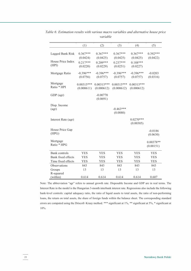
Narodowy Bank Polski28
27
Table 6: Estimation results with various macro variables and alternative house price variable
(1) (2) (3) (4) (5) Lagged Bank Risk 0.367*** 0.367*** 0.367*** 0.367*** 0.392*** (0.0424) (0.0425) (0.0425) (0.0425) (0.0422) House Price Index (HPI)
0.217*** 0.209*** 0.237*** 0.188*** (0.0220) (0.0229) (0.0251) (0.0227)
Mortgage Ratio -0.396*** -0.396*** -0.396*** -0.396*** -0.0203 (0.0756) (0.0757) (0.0757) (0.0757) (0.0316)
Mortgage Ratio * HPI
0.00315*** 0.00315*** 0.00315*** 0.00315*** (0.000611) (0.000612) (0.000612) (0.000612)
GDP (agr) -0.00770 (0.0691)
Disp. Income (agr) -0.463*** (0.0880)
Interest Rate (agr) 0.0270*** (0.00305)
House Price Gap (HPG)
-0.0186 (0.0630)
Mortgage Ratio * HPG
0.00378**
(0.00151)
Bank controls YES YES YES YES YES Bank fixed effects YES YES YES YES YES Time fixed effects YES YES YES YES YES Observations 843 843 843 843 843 Groups 13 13 13 13 13 R-squared (within) 0.614 0.614 0.614 0.614 0.607
Note: The abbreviation “agr” refers to annual growth rate. Disposable Income and GDP are in real terms. The
Interest Rate in the model is the Hungarian 3-month interbank interest rate. Regressions also include the following
bank-level controls: capital adequacy ratio, the ratio of liquid assets to total assets, the ratio of non-performing
loans, the return on total assets, the share of foreign funds within the balance sheet. The corresponding standard
errors are computed using the Driscoll–Kraay method. *** significant at 1%, ** significant at 5%, * significant at
10%.

29NBP Working Paper No. 289
Appendix
27
Table 6: Estimation results with various macro variables and alternative house price variable
(1) (2) (3) (4) (5) Lagged Bank Risk 0.367*** 0.367*** 0.367*** 0.367*** 0.392*** (0.0424) (0.0425) (0.0425) (0.0425) (0.0422) House Price Index (HPI)
0.217*** 0.209*** 0.237*** 0.188*** (0.0220) (0.0229) (0.0251) (0.0227)
Mortgage Ratio -0.396*** -0.396*** -0.396*** -0.396*** -0.0203 (0.0756) (0.0757) (0.0757) (0.0757) (0.0316)
Mortgage Ratio * HPI
0.00315*** 0.00315*** 0.00315*** 0.00315*** (0.000611) (0.000612) (0.000612) (0.000612)
GDP (agr) -0.00770 (0.0691)
Disp. Income (agr) -0.463*** (0.0880)
Interest Rate (agr) 0.0270*** (0.00305)
House Price Gap (HPG)
-0.0186 (0.0630)
Mortgage Ratio * HPG
0.00378**
(0.00151)
Bank controls YES YES YES YES YES Bank fixed effects YES YES YES YES YES Time fixed effects YES YES YES YES YES Observations 843 843 843 843 843 Groups 13 13 13 13 13 R-squared (within) 0.614 0.614 0.614 0.614 0.607
Note: The abbreviation “agr” refers to annual growth rate. Disposable Income and GDP are in real terms. The
Interest Rate in the model is the Hungarian 3-month interbank interest rate. Regressions also include the following
bank-level controls: capital adequacy ratio, the ratio of liquid assets to total assets, the ratio of non-performing
loans, the return on total assets, the share of foreign funds within the balance sheet. The corresponding standard
errors are computed using the Driscoll–Kraay method. *** significant at 1%, ** significant at 5%, * significant at
10%.
28
Figure 7: Partial effect of the House Price Gap on bank risk
Figure 8: Partial effect of the mortgage loan ratio on bank risk for the model including the House Price Gap
-0.05
0
0.05
0.1
0.15
0.2
0.25
0.3
0.35
0.4
-0.05
0
0.05
0.1
0.15
0.2
0.25
0.3
0.35
0.4
0 5 10 15 20 25 30 35 40 45 50 55 60 65 70 75 80 85 90 95 100
Size
of t
he p
artia
l effe
ct
Mortgage loan ratio
-0.1
-0.08
-0.06
-0.04
-0.02
0
0.02
0.04
0.06
-0.1
-0.08
-0.06
-0.04
-0.02
0
0.02
0.04
0.06
-17-15-13-11 -9 -7 -5 -3 -1 1 3 5 7 9 11 13 15 17
Size
of t
he p
artia
l effe
ct
House Price Gap

Narodowy Bank Polski30
29
Table 7: Estimation results with different risk measures
(1) (2) (3) (4) (5) (6) Dynamic Static Lagged EBA-risk
0.367*** (0.0424)
House Price Index (HPI)
0.217*** 0.258*** -0.000395 0.320*** 0.420*** 0.0164*** (0.0220) (0.0283) (0.000950) (0.0195) (0.0211) (0.00268)
Mortgage Ratio
-0.396*** -0.343*** 0.00533 -0.614*** -0.567*** 0.135*** (0.0756) (0.0817) (0.00331) (0.0923) (0.113) (0.0144)
Mortgage Ratio * HPI 0.00315*** 0.00199*** -4.85e-05* 0.00499*** 0.00345***
-0.00131***
(0.000611) (0.000646) (2.86e-05) (0.000784) (0.000973) (0.000136)
Lagged EBA-risk (E)
0.420*** (0.0460)
Lagged Z-risk
0.909*** (0.0221)
Bank controls YES YES YES YES YES YES Bank FE YES YES YES YES YES YES Time FE YES YES YES YES YES YES Observations 843 843 842 843 843 843 Groups 13 13 13 13 13 13 R-squared (within)
0.614 0.637 0.975 0.546 0.547 0.482
Note: (E) indicates: equal weights. Regressions also include the following bank-level controls: capital adequacy
ratio, the ratio of liquid assets to total assets, the ratio of non-performing loans, the return on total assets, the share
of foreign funds within the balance sheet. The corresponding standard errors are computed using the Driscoll–
Kraay method. *** significant at 1%, ** significant at 5%, * significant at 10%.

31NBP Working Paper No. 289
Appendix
29
Table 7: Estimation results with different risk measures
(1) (2) (3) (4) (5) (6) Dynamic Static Lagged EBA-risk
0.367*** (0.0424)
House Price Index (HPI)
0.217*** 0.258*** -0.000395 0.320*** 0.420*** 0.0164*** (0.0220) (0.0283) (0.000950) (0.0195) (0.0211) (0.00268)
Mortgage Ratio
-0.396*** -0.343*** 0.00533 -0.614*** -0.567*** 0.135*** (0.0756) (0.0817) (0.00331) (0.0923) (0.113) (0.0144)
Mortgage Ratio * HPI 0.00315*** 0.00199*** -4.85e-05* 0.00499*** 0.00345***
-0.00131***
(0.000611) (0.000646) (2.86e-05) (0.000784) (0.000973) (0.000136)
Lagged EBA-risk (E)
0.420*** (0.0460)
Lagged Z-risk
0.909*** (0.0221)
Bank controls YES YES YES YES YES YES Bank FE YES YES YES YES YES YES Time FE YES YES YES YES YES YES Observations 843 843 842 843 843 843 Groups 13 13 13 13 13 13 R-squared (within)
0.614 0.637 0.975 0.546 0.547 0.482
Note: (E) indicates: equal weights. Regressions also include the following bank-level controls: capital adequacy
ratio, the ratio of liquid assets to total assets, the ratio of non-performing loans, the return on total assets, the share
of foreign funds within the balance sheet. The corresponding standard errors are computed using the Driscoll–
Kraay method. *** significant at 1%, ** significant at 5%, * significant at 10%.
30
Table 8: Estimation results of models with various mortgage exposure limits
(1) (2) (3) (4) Lagged Bank Risk 0.351*** 0.386*** 0.388*** 0.383*** (0.0443) (0.0416) (0.0415) (0.0411) House Price Index (HPI) 0.226*** 0.212*** 0.211*** 0.216*** (0.0213) (0.0208) (0.0203) (0.0208) Mortgage Ratio >25% -20.71*** (4.126) Mortgage Ratio >25% * HPI 0.178*** (0.0370) Mortgage Ratio >30% -12.74*** (3.241) Mortgage Ratio >30% * HPI 0.104*** (0.0298) Mortgage Ratio >35% -10.07*** (3.182) Mortgage Ratio >35% * HPI 0.0956*** (0.0312) Mortgage Ratio >40% -10.86*** (2.894) Mortgage Ratio >40% * HPI 0.100*** (0.0258) Bank controls YES YES YES YES Bank fixed effects YES YES YES YES Time fixed effects YES YES YES YES Number of observations 843 843 843 843 Number of groups 13 13 13 13 R-squared (within) 0.617 0.610 0.609 0.609
Note: Regressions also include the following bank-level controls: capital adequacy ratio, the ratio of liquid assets
to total assets, the ratio of non-performing loans, the return on total assets, the share of foreign funds within the
balance sheet. The corresponding standard errors are computed using the Driscoll–Kraay method. *** significant
at 1%, ** significant at 5%, * significant at 10%.
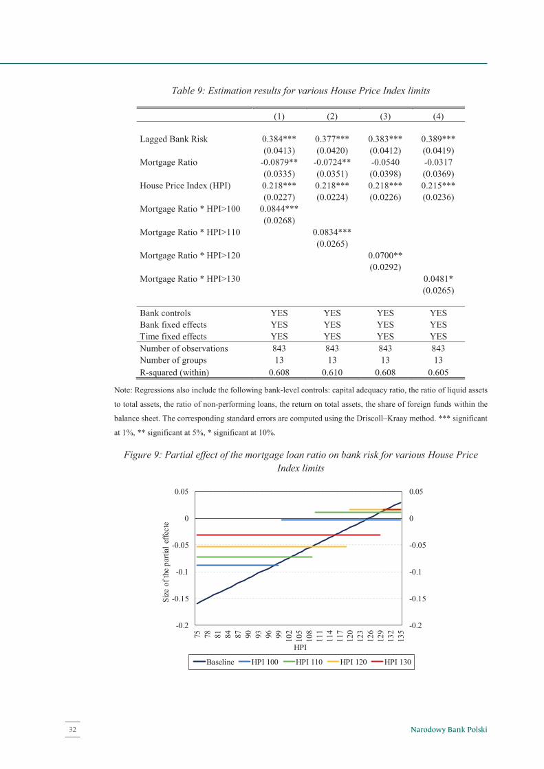
Narodowy Bank Polski32
31
Table 9: Estimation results for various House Price Index limits
(1) (2) (3) (4) Lagged Bank Risk 0.384*** 0.377*** 0.383*** 0.389*** (0.0413) (0.0420) (0.0412) (0.0419) Mortgage Ratio -0.0879** -0.0724** -0.0540 -0.0317 (0.0335) (0.0351) (0.0398) (0.0369) House Price Index (HPI) 0.218*** 0.218*** 0.218*** 0.215*** (0.0227) (0.0224) (0.0226) (0.0236) Mortgage Ratio * HPI>100 0.0844*** (0.0268) Mortgage Ratio * HPI>110 0.0834*** (0.0265) Mortgage Ratio * HPI>120 0.0700** (0.0292) Mortgage Ratio * HPI>130 0.0481* (0.0265) Bank controls YES YES YES YES Bank fixed effects YES YES YES YES Time fixed effects YES YES YES YES Number of observations 843 843 843 843 Number of groups 13 13 13 13 R-squared (within) 0.608 0.610 0.608 0.605
Note: Regressions also include the following bank-level controls: capital adequacy ratio, the ratio of liquid assets
to total assets, the ratio of non-performing loans, the return on total assets, the share of foreign funds within the
balance sheet. The corresponding standard errors are computed using the Driscoll–Kraay method. *** significant
at 1%, ** significant at 5%, * significant at 10%.
Figure 9: Partial effect of the mortgage loan ratio on bank risk for various House Price Index limits
-0.2
-0.15
-0.1
-0.05
0
0.05
-0.2
-0.15
-0.1
-0.05
0
0.05
75 78 81 84 87 90 93 96 99 102
105
108
111
114
117
120
123
126
129
132
135
Size
of t
he p
artia
l effe
cte
HPI
Baseline HPI 100 HPI 110 HPI 120 HPI 130

33NBP Working Paper No. 289
Appendix
31
Table 9: Estimation results for various House Price Index limits
(1) (2) (3) (4) Lagged Bank Risk 0.384*** 0.377*** 0.383*** 0.389*** (0.0413) (0.0420) (0.0412) (0.0419) Mortgage Ratio -0.0879** -0.0724** -0.0540 -0.0317 (0.0335) (0.0351) (0.0398) (0.0369) House Price Index (HPI) 0.218*** 0.218*** 0.218*** 0.215*** (0.0227) (0.0224) (0.0226) (0.0236) Mortgage Ratio * HPI>100 0.0844*** (0.0268) Mortgage Ratio * HPI>110 0.0834*** (0.0265) Mortgage Ratio * HPI>120 0.0700** (0.0292) Mortgage Ratio * HPI>130 0.0481* (0.0265) Bank controls YES YES YES YES Bank fixed effects YES YES YES YES Time fixed effects YES YES YES YES Number of observations 843 843 843 843 Number of groups 13 13 13 13 R-squared (within) 0.608 0.610 0.608 0.605
Note: Regressions also include the following bank-level controls: capital adequacy ratio, the ratio of liquid assets
to total assets, the ratio of non-performing loans, the return on total assets, the share of foreign funds within the
balance sheet. The corresponding standard errors are computed using the Driscoll–Kraay method. *** significant
at 1%, ** significant at 5%, * significant at 10%.
Figure 9: Partial effect of the mortgage loan ratio on bank risk for various House Price Index limits
-0.2
-0.15
-0.1
-0.05
0
0.05
-0.2
-0.15
-0.1
-0.05
0
0.05
75 78 81 84 87 90 93 96 99 102
105
108
111
114
117
120
123
126
129
132
135
Size
of t
he p
artia
l effe
cte
HPI
Baseline HPI 100 HPI 110 HPI 120 HPI 130
32
Table 10: Results obtained by different estimation methods
(1) (2) (3) (4) (5) (6) Estimator: Within LSDV Within LSDV LSDVC Within St. Error: DK DK Robust Robust Bootstrap DK
Lagged Bank Risk
0.367*** 0.367*** 0.367*** 0.367*** 0.391*** 0.578*** (0.0424) (0.0428) (0.0570) (0.0400) (0.0337) (0.0341)
Mortgage Ratio
-0.396*** -0.396*** -0.396*** -0.396*** -0.391*** -0.146** (0.0756) (0.0762) (0.0948) (0.0862) (0.116) (0.0702)
House Price Index (HPI)
0.217*** 0.192*** 0.0565 0.0565 -0.140 0.119*** (0.0220) (0.0211) (0.0596) (0.0499) (0.538) (0.00988)
Mortgage Ratio * HPI
0.00315*** 0.00315*** 0.00315*** 0.00315*** 0.00308*** 0.00183*** (0.000611) (0.000616) (0.000684) (0.000704) (0.000908) (0.000470)
Bank controls YES YES YES YES YES NO Bank FE YES YES YES YES YES YES Time FE YES YES YES YES YES YES Observations 843 843 843 843 843 843 Groups 13 13 13 13 13 13 R-squared (within)
0.614 - 0.614 - - 0.534
R-squared - 0.7821 - 0.758 - -
Note: DK indicates: Driscoll-Kraay. Regressions also include the following bank-level controls: capital adequacy
ratio, the ratio of liquid assets to total assets, the ratio of non-performing loans, the return on total assets, the share
of foreign funds within the balance sheet. The corresponding standard errors are computed using the Driscoll–
Kraay method. *** significant at 1%, ** significant at 5%, * significant at 10%.

Narodowy Bank Polski34
33
Figure 10: Partial effect of house prices on bank risk in models estimated by different
methods
Figure 11: Partial effect of the mortgage loan ratio on bank risk in models estimated by different methods
0
0.1
0.2
0.3
0.4
0.5
0.6
0
0.1
0.2
0.3
0.4
0.5
0.6
0 5 10 15 20 25 30 35 40 45 50 55 60 65 70 75 80 85 90 95 100
Size
of t
he p
artia
l effe
ct
Mortgage ratioWithin (DK) LSDV (DK) LSDVCLSDV (robust) Within (robust)
-0.2
-0.15
-0.1
-0.05
0
0.05
0.1
-0.2
-0.15
-0.1
-0.05
0
0.05
0.1
75 80 85 90 95 100 105 110 115 120 125 130 135
Size
of t
he p
artia
l effe
ct
HPIWithin (DK) LSDV (DK) LSDVCLSDV (robust) Within (robust)

www.nbp.pl


![[Longstaff] Electricity Forward Prices - A High Frequency Empirical Analysis](https://img.pdfslide.us/doc/110x75/577cdf411a28ab9e78b0ce0d/longstaff-electricity-forward-prices-a-high-frequency-empirical-analysis.jpg)