Louisiana State UniversityLSU Digital Commons

LSU Historical Dissertations and Theses Graduate School

1984

An Empirical Investigation of the Effect of CapitalStructure Regulation on the Asset Portfolio ofCommercial Banks.Robert Edward LamyLouisiana State University and Agricultural & Mechanical College

Follow this and additional works at: https://digitalcommons.lsu.edu/gradschool_disstheses

This Dissertation is brought to you for free and open access by the Graduate School at LSU Digital Commons. It has been accepted for inclusion inLSU Historical Dissertations and Theses by an authorized administrator of LSU Digital Commons. For more information, please contactgradetd@lsu.edu.

Recommended CitationLamy, Robert Edward, "An Empirical Investigation of the Effect of Capital Structure Regulation on the Asset Portfolio of CommercialBanks." (1984). LSU Historical Dissertations and Theses. 3963.https://digitalcommons.lsu.edu/gradschool_disstheses/3963

INFORMATION TO USERS

This reproduction was m ade from a copy o f a docum ent sent to us fo r microfilming. While the m ost advanced technology has been used to photograph and reproduce this docum ent, the quality o f the reproduction is heavily dependent upon the quality o f the m aterial subm itted.

The following explanation o f techniques is provided to help clarify markings or notations which may appear on this reproduction.

1 .T he sign or “ target” for pages apparently lacking from the docum ent photographed is “ Missing Page(s)” . I f it was possible to obtain the missing page(s) or section, they are spliced in to the film along w ith adjacent pages. This may have necessitated cutting through an image and duplicating adjacent pages to assure com plete continuity .

2. When an image on the film is obliterated with a round black mark, it is an indication o f e ither blurred copy because o f m ovem ent during exposure, duplicate copy, or copyrighted m aterials th a t should n o t have been filmed. For blurred pages, a good image o f the page can be found in the adjacent frame. If copyrighted materials were deleted, a target note will appear listing the pages in the adjacent frame.

3. When a map, drawing or chart, etc ., is part o f the m aterial being photographed, a definite m ethod o f “sectioning” the m aterial has been followed. It is custom ary to begin filming at the upper left hand com er o f a large sheet and to continue from left to right in equal sections with small overlaps. If necessary, sectioning is continued again—beginning below the first row and continuing on until com plete.

4. For illustrations tha t cannot be satisfactorily reproduced by xerographic means, photographic prints can be purchased at additional cost and inserted into your xerographic copy. These prints are available upon request from the Dissertations Custom er Services D epartm ent.

5. Some pages in any docum ent may have indistinct print. In all cases the best available copy has been filmed.

UniversityM o c x i lm s

International300 N. Zeeb Road Ann Arbor, Ml 48106

8425878

Lamy, Robert Edward

AN EMPIRICAL INVESTIGATION OF THE EFFECT OF CAPITAL STRUCTURE REGULATION ON THE ASSET PORTFOLIO OF COMMERCIAL BANKS

The Louis iana Stale University and A g r ic u l tu ra l a n d M echan ica l Col. Ph.D. 1984

University Microfilms

International 300 N. Zeeb Road, Ann Arbor, Ml 48106

PLEASE NOTE:

In all c a s e s this material has been filmed in the best possible way from the available copy. Problems encountered with this docum ent have been identified here with a check mark V .

1. G lossy photographs or p a g e s_______

2. Colored illustrations, paper or print______

3. Photographs with dark background______

4. Illustrations are poor c o p y _______

5. P ages with black marks, not original copy__

6. Print shows through as there is text on both s id es of page_______

7. Indistinct, broken or small print on several p a g e s ^

8. Print exceed s margin requirem ents______

9. Tightly bound copy with print lost in spine_______

10. Computer printout pages with indistinct print_______

11. P a g e(s)_____________ lacking when material received, and not available from school orauthor.

12. P age(s)_____________ seem to be missing in numbering only a s text follows.

13. Two pages num bered_____________ . Text follows.

14. Curling and wrinkled p a g e s_______

15. Other_________________________________________________________ _

UniversityMicrofilms

International

AN EMPIRICAL INVESTIGATION OF THE EFFECT OF CAPITAL STRUCTURE REGULATION ON THE ASSET PORTFOLIO

OF COMMERCIAL BANKS

A DissertationSubmitted to the Graduate Faculty of the

Louisiana State University and Agricultural and Mechanical College

in partial fulfillment of the the requirements for the degree of

Doctor of Philosophyin

Finance

by

Robert Edward LamyB.S., Southeastern Louisiana University, 1974

M.B.A., Southeastern Louisiana University, 1976May, 1984

ACKNOWLEDGEMENT S

This dissertation is the product of many hours of determined effort and I would like to express my graditude to those who were an integral part of its completion. I thank Dr. Charles G. Martin, who I have had the honor to be associated with my entire doctoral program at Louisiana State University. Not only did he provide the idea for this dissertation but his unendless support and guidence on this project is a debt I will never be able to repay. I also wish to thank the others members of my committee for their insight and help: Dr. William R. Lane, Associate Professor of Finance; Dr. David T. Crary, Professor of Finance; Dr. C. F. Sirmans; Dr. David Cordell, Assistant Professor of Finance; and Dr. Jefferey Ringuest, Assistant Professor of Quantitative Business Analysis. My sincere thanks also go to my family and friends whom, without their support, this dissertation would be yet unfinished.

Finally, I would like to dedicate this dissertation to my wife, Amy, and my daughter, Meredith. Their unselfish devotion, patience and understanding has made this endeavor a true joy. My appreciation comes from the bottom of my heart.

TABLE OF CONTENTS

ACKNOWLEDGEMENTS ........................................... iiLIST OF T A B L E S ............................................... viLIST OF FIGURES ............................................viiA B S T R A C T ............. viii

Chapterpage

I. INTRODUCTION ......................................... 1Purpose of Regulation of Commercial Banks . . . 1Capital Regulation of Commercial Banks ......... 2Previous Research Relating to Capital Adequacy . 4Theory of Bank's Reaction to Capital Regulation 5 Outline of the S t u d y ................................ 5

II. MODELS OF THE BANKING F I R M ............................7Introduction ....................................... 7The Decision-Making Process of Unregulated Banks 8Assumptions of Swary's Model .................... 9The Investment Decision of the B a n k ............. 12The Financing Decision ........................... 18D e p o s i t s ............................................. 18Purchased Funds .................................. 18E q u i t y ............................................... 19Financing Decision: Selecting the Optimal

Capital Structure ......................... 19Banks Decision Making Process Under Regulation . 23Normative Case:Direct Chance Constraint...........24Descriptive Model--Capital Regulation ......... 25Bank Reaction to Capital Regulation............... 29Koehn-Santomero Portfolio Investment Model . . . 30A s s u m p t i o n s ........................................ 30The Individual Banks Utility Function............. 33The Reaction of Bank to Capital Regulation . . . 36 O'Hara's Dynamic Theory of the Banking Firm. . . 38S u m m a r y ............................................. 41

III. CAPITAL REGULATION AND BANKRUPTCY RISK ........... 43Introduction ...................................... 43Scott-Edwards Bankruptcy Probability ........... 44Parameter Shifts and Bankruptcy Probability . . 49A Change in Mean of the Distribution of X . . . 50 A Change in Both the Mean and Standard Deviation

of X .......................................... 51A Change in the Standard Deviation of X Holding

Mean C o n s t a n t ............................. .-52Capital Regulation and Bankruptcy Risk ......... 53Bankruptcy Risk in the Koehn <& Santomero Model . 57

IV. ' SAMPLE SELECTION AND EMPIRICAL TEST DESIGN . . . . 64Introduction ....................................... 64Formal Statement of the Hypotheses ............. 65Sample Selection .................................. 67Regulatory Environment ........................... 67Data A v a i l a b i l i t y ................................. 68Capital Structure Shift ......................... 69Survey Results .................................... 70Questionnaire Results ........................... 70The Regulated Sample ............................. 72Matched-Pair Sample........... 74Test Methodology....................................76Univariate Tests .................................. 78Multivariate Tests ................................ 80Analysis of Variance ............................. 80Reshuffling Test Design ......................... 81Default-Risk Model ................................ 83S u m m a r y ..................... '...................... 86

V. EMPIRICAL RESULTS .................................... 88Introduction ....................................... 88Univariate Tests .................................. 89Multivariate T e s t ................................ 101

Test of Reshuffling Hypothesis ........... 101Loan Portfolio Reshuffling ................ 107Additional Assumptions of the Model . . . . 114

Default Risk Hypothesis ....................... 116VI. SUMMARY, LIMITATIONS, AND CONCLUSIONS ........... 122

iv

Appendicespage

A. UNIVARIATE STATISTICS .............................. 132B. LIST OF BANKS IN S A M P L E .............................. 150C. V I T A ..................................................... 154

v

LIST OF TABLES

Tablepage

1. Survey Response R a t e .................................... 722. Response to Bank Type Code/By Y e a r .................... 733. Summary Statistics - Means ............................ 744. Summary Statistics - Means ............................ 765. Assets Portfolio and Profitability Variables . . . . 776. Results of Univariate "t" t e s t s ...................... 937. Summary of Univariate Tests ....................... 1008. Results of Reshuffling Hypothesis Tests ........... 1039. Results of Risk-Return Reshuffling of Loan

Por t f o l i o....................................... Ill10. Regression Results of Default-Risk Hypothesis . . 119

vi

LIST OF FIGURES

FigurePage

1. Figure 1 .................................................. 162. Figure 2 .................................................. 463. Figure 3 .................................................. 59

vii

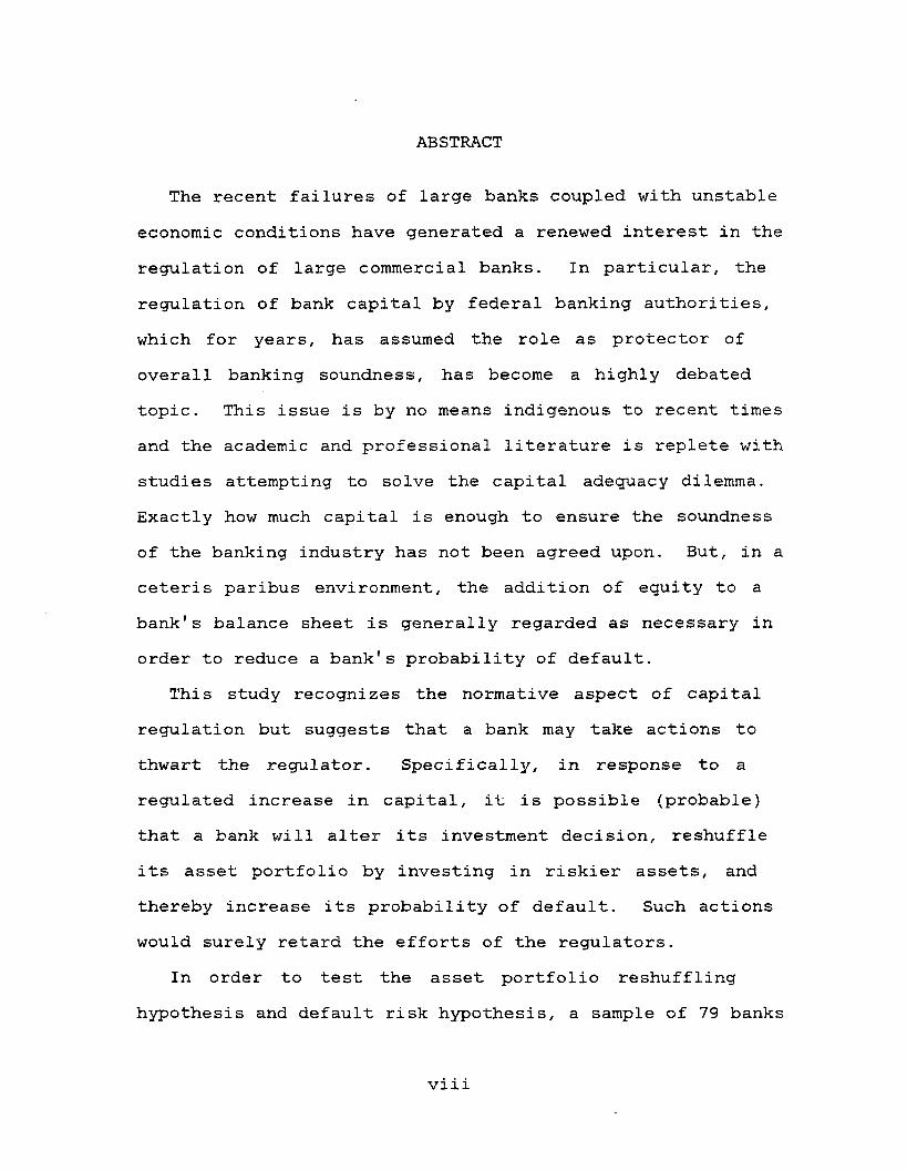
ABSTRACT

The recent failures of large banks coupled with unstable economic conditions have generated a renewed interest in the regulation of large commercial banks. In particular, the regulation of bank capital by federal banking authorities, which for years, has assumed the role as protector of overall banking soundness, has become a highly debated topic. This issue is by no means indigenous to recent times and the academic and professional literature is replete with studies attempting to solve the capital adequacy dilemma. Exactly how much capital is enough to ensure the soundness of the banking industry has not been agreed upon. But, in a ceteris paribus environment, the addition of equity to a bank's balance sheet is generally regarded as necessary in order to reduce a bank's probability of default.

This study recognizes the normative aspect of capital regulation but suggests that a bank may take actions to thwart the regulator. Specifically, in response to a regulated increase in capital, it is possible (probable) that a bank will alter its investment decision, reshuffle its asset portfolio by investing in riskier assets, and thereby increase its probability of default. Such actions would surely retard the efforts of the regulators.

In order to test the asset portfolio reshuffling hypothesis and default risk hypothesis, a sample of 79 banks

viii

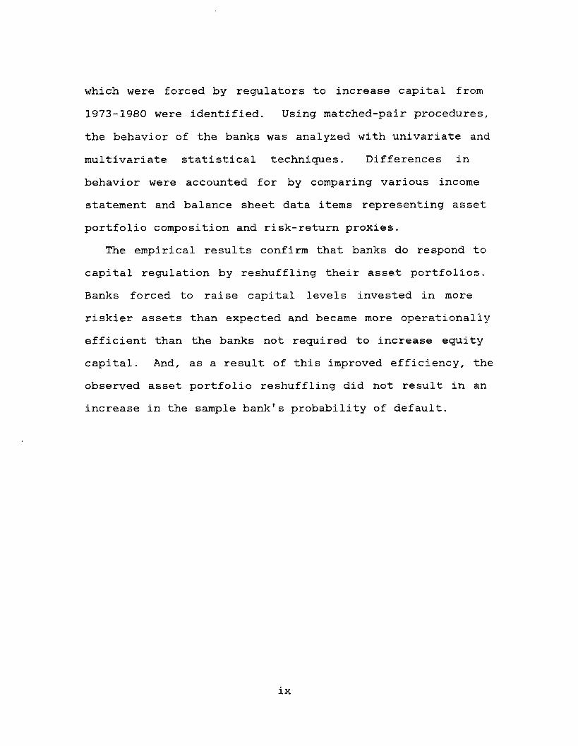
which were forced by regulators to increase capital from 1973-1980 were identified. Using matched-pair procedures, the behavior of the banks was analyzed with univariate and multivariate statistical techniques. Differences in behavior were accounted for by comparing various income statement and balance sheet data items representing asset portfolio composition and risk-return proxies.

The empirical results confirm that banks do respond to capital regulation by reshuffling their asset portfolios. Banks forced to raise capital levels invested in more riskier assets than expected and became more operationally efficient than the banks not required to increase equity capital. And, as a result of this improved efficiency, the observed asset portfolio reshuffling did not result in an increase in the sample bank's probability of default.

ix

Chapter I INTRODUCTION

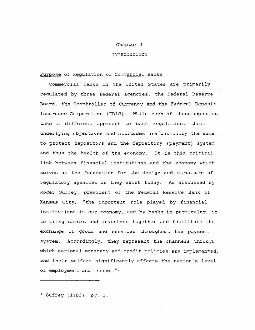
Purpose of Regulation of Commercial BanksCommercial banks in the United States are primarily

regulated by three federal agencies: the Federal ReserveBoard, the Comptroller of Currency and the Federal Deposit Insurance Corporation (FDIC). While each of these agencies take a different approach to bank regulation, their underlying objectives and attitudes are basically the same, to protect depositors and the depository (payment) system and thus the health of the economy. It is this critical link between financial institutions and the economy which serves as the foundation for the design and structure of regulatory agencies as they exist today. As discussed by Roger Guffey, president of the Federal Reserve Bank of Kansas City, "the important role played by financial institutions in our economy, and by banks in particular, is to bring savers and investors together and facilitate the exchange of goods and services throughout the payment system. Accordingly, they represent the channels through which national monetary and credit policies are implemented, and their welfare significantly affects the nation's level of employment and income."1

1 Guffey (1983), pg. 3.

2As purported by various authors, Meltzer (1967),

Bentson (1973), and Black, Miller and Posner (1978), the existence of regulation of commercial banks is desired for two reasons:2

1. Because of the imperfect transmission of information, bank depositors (customers) are at times uninformed of the decisions or the financial condition of a bank. And it is felt that Federal authorities can monitor (examine) and regulate the system more effectively and efficiently.

2. Social costs as a result of a fall in public confidence of the banking system far outweigh the actual cost of the implementation of such a system. For example, deposit insurance serves to prevent bank failures, and associated costs, resulting from deposit runs. Thus, the FDIC simultaneously protects the nation's and its own interest.

Capital Regulation of Commercial BanksThis study focuses its attention on one major form of

bank regulation - the regulation of equity capital. Equity capital and the probability of bank failure are related on a direct, fundamental level. "The primary function of equity capital has been considered to be the protection of depositors. The protective function has been viewed not only as assuring payoff of depositors in the case of liquidation but also contributing to the maintainence of solvency by providing a cushion of excess assets so

2 See Posner (1974) or Peltzman (1970) for a review of economic theories of regulation.

that a bank threatened with losses might continue in operation".3 Given a level of equity capital, the states of nature in which bankruptcy will occur are those where Assets - Liabilities = Equity < 0, and the higher the level of capital, ceteris paribus, the less risk depositors assume.

Capital regulation does have potential drawbacks however. In particular, restricting the use of financial leverage, debt/equity, reduces the rates of return on equity available to the bank. It is feared that this may retard the flow of investment dollars into the banking industry and eventually have a dampening affect on overall economic growth.

The three major forms of regulation faced by commercial banks are portfolio restrictions, Regulation Q, and capital requirements. Of these, the latter is the most controversial due to the imprecise nature of measuring and enforcing capital standards. Traditionally the three agencies have used rather informal guidelines to determine an adequate level of capital. Futhermore, the standard and thecomputation procedure differed across this triumvirate. Vojta (1973) reports that the Federal Reserve Board assigns different capital requirements to each class of assets according to its perceived risk. The Comptroller ofCurrency evaluates management and asset quality in conjuction with the bank's deposit base to appraise

3 Reed, Cotter, Gill and Smith (1980), pg. 154.

necessary capital. The FDIC' relies on a ratio of equity to total assets, net of fixed and substandard assets, and employs this measure in the regulation of all commercial banks.4

Previous Research Relating to Capital AdequacyPrevious research in the area of capital adequacy has

primarily focused on:1. Who should regulate capital? Or the issue of Optimal

vs. Adequate capital.52. How should capital standards be established? Or,how

effective is the present regime of capital regulation? 6

3. What are the costs resulting from inadequate capital? Analysis of the social costs and benefits of government regulation.7

Limited attention, however, has been given to the possiblereaction by commercial banks to capital adequacy regulation.Assuming that capital regulation is exogenous to thedecision-making process of the commercial bank, as is thecase presently, how may a bank be expected to respond tosuch regulation?

4 See Vojta (1973), pg. 1-15.5 See Robinson and Pettway (1967), Pringle (1974) and

Taggart and Greenbaum (1978).6 See Mayne (1972), Peltzman (1970) and Mingo (1975).7 See Santomero and Watson (1977).

5Theory of Bank1s Reaction to- Capital Regulation

Theoretic studies by Swary (1979), Koehn and Santomero (1980), Edwards and Scott (1977) and O'Hara (1983), have directly or indirectly analyzed this question and suggest that in response to capital regulation a commercial bank may be expected to reshuffle its asset portfolio into riskier assets. Further, it is hypothesized that as a result of asset reshuffling the bank may actually increase its probability of bankruptcy. Such a result is, of course, contrary to the soundness objective of regulators. To date, however, this joint hypothesis has not been empirically tested. Thus, the objective of this study is to determine if banks required by regulators to increase equity capital do in fact reshuffle their asset portfolios, and as a result of any reshuffling increase their risk of bankruptcy.

Outline of the StudyAnalysis of the reshuffling and bankruptcy hypotheses

proceeds in the following steps.Chapter Two summarizes the models of Swary, Koehn and

Santomero, and O'Hara which analyze the decision-making process of the commercial bank both in an unregulated and regulated environment. Special emphasis is given to the impact of an exogenous increase in equity capital on this process.

Chapter Three introduces Scott and Edwards' and Koehn and Santomero's models of bankruptcy risk into the decision-making models and looks at how the reshuffling hypothesis is related to the probability of bankruptcy.

Chapter Four describes the sample of regulated and unregulated banks to be used in the examination of the proposed hypotheses. In addition, the design of the empirical test employed is derived in this chapter.

Chapter Five presents the empirical results of both the reshuffling and bankruptcy risk hypotheses along with some statistical insight into the identification process of an undercapitalized bank by regulators.

Chapter Six provides a summary of the results and areas for further research.

Chapter II MODELS OF THE BANKING FIRM

IntroductionThe need for artificially regulated levels of equity

capital of the financial intermediary stems from the theory that equity capital provides a cushion against unplanned financial difficulties, reduces the probability of default and, in effect, acts as a protective buffer for both the individual depositor and the banking system as a whole. However, as has been suggested by Koehn and Santomero (1980), Blair and Heggestad (1978), Swary (1980), Scott and Edwards (1977), Kahane (1977) and O ’Hara (1983), the intent of the capital regulation is reasonable but may be ineffectual. While the belief that increases in equity capital reduce the probability of default may have merit, the possibility also exists that, in reaction to this regulated change in capital structure, the intermediary may engage in actions which actually increase the risk or probability of default.

This chapter attempts to analyze the effect of capital regulation upon the decision-making process of the commercial bank by discussing Swary's model of the bank in an unregulated environment and comparing these results to his model of the banking firm under capital regulation. The

portfolio model approach of Koehn and Santomero is also discussed with particular emphasis given to the relationship between capital regulation and the optimal asset portfolio decision of the commercial bank. Finally, a dynamic analysis approach to the banking firm developed by O'Hara is examined. The findings are then viewed in terms of default probability to measure the overall effectiveness of capital regulation.

The Decision-Making Process of Unregulated BanksSwary's research in the area of capital adequacy

primarily focused on the regulation of bank holding companies but provides a rather useful model of the behavior of commercial banks. As Swary points out, the mere existence of banks is based upon uncertainty and imperfections in the capital markets with regard to the collecting and processing of information. Therefore, it must be assumed that banks possess comparative advantages in securing and disseminating information, which explains their presence in capital markets and their ability to provide financial services more economically. Swary1s model incorporates uncertainty, costs of information, and probability of failure in modeling the investment (allocation of credit) and financing decisions of the unregulated commercial bank.

Assumptions of Swary' s Model-The commercial bank is viewed as an economic entity

possessing typical firm behavior in the microeconomic sense,i.e., inputs, outputs, pricing, etc.8 It is assumed that the bank attempts to maximize an objective function, expressed in terms of market value, in relation to the equilibrium valuation function. The overriding characteristic of the valuation function is a linear relationship between the returns from any two financial variables, i.e., the market value of any given return distribution (generated by investments) is set equal to the sum of the individual return distributions.9

In contrast to the typical assumptions of insignificant bankruptcy costs, as suggested by Warner (1977), Baxter (1967) and others, any analysis in the banking area must surely recognize positive bankruptcy costs. While there may be an argument for zero direct bankruptcy costs, i.e., reorganization costs (the costs measured by Warner in his study of bankrupt railroads), dismissing relevant indirect bankruptcy costs for financial firms, especially the disruption of the bank's production process and the supplier

8 Most studies in this area treat the individual bank as an investor maximizing expected utility. For example, Porter (1961), Klein (1971), Michealsen and Goshay (1967) and Pyle (1972).

9 Given competitive markets, arbitrage considerations result in this property. See Ross (1976).

10- customer. relationship may be questionable10 As Swary points out, "indirect costs of bankruptcy are likely to be of paramount importance in the banking industry for the following reasons:

1. Given the existence of restrictions on entry to the industry, the charter of a bank has a market value. Should a bank fail, the market value of the charter will be reduced because of direct regulation intervention in acquisitions and mergers.

2. Even if entry of firms were not restricted, a bank's investment in goodwill would be substantially lost should it fail.

3. Regulatory authorities are sensitive to the likelihood of bankruptcy. Therefore, regulators are likely to impose additional constraints (costs) on the bank when the probability of bankruptcy goes beyond a certain level."11

10 See Baxter (1967).11 Swary (1980), pg. 12.

11Balance Sheet

The bank issues three types of liabilities: deposits,money market instruments and common equity; two types of assets: loans and investment securities, and is constrainedby the balance sheet identity:

where:C = common equity funds endogeneously determined.F = money market (federal funds) funds which are short

term and interest bearing, (F>0).Dm = deposits, m = 1, , M, which are exogenous

and stochastic.= loans purchased by the bank, i = 1, ... , N.

The bank is assumed to control equity, borrowed funds and loans purchased in a heterogenous market with respect to underlying credit risk. The bank decides on loans and equity capital at the beginning of the period. Immediatelyafter these decision variables are determined, changes occur

}in the money market funds' interest rates and deposit inflows, which require compensating adjustments in borrowing in order to satisfy the balance sheet constraint. The

MC + F" +

M N(1)

12resulting levels of loans, deposits, borrowing, and capital then remain constant until the end of the period.

The Investment Decision of the Bank

The actual credit extension process (investment decision) of the bank is somewhat different from its counterparts in non-financial industries. In particular, the loan agreement is much more specific and binding than contractual arrangements in the bond market. The bank, in fact, circumvents the third party arrangement of the trustee, which not only improves the customer relationship, but also allows the bank to provide and receive payment for servicing the loan. By acting as the trustee of the loan agreement, the commercial bank has succeeded in resolving, to some extent, the uncertainty of loan default and also obtains information valuable to future credit decisions. This inventory of information enables banks to provide these financial services more economically than other markets. In addition, unless banks possess a comparative advantage in producing these financial goods, they would not invest in an asset, such as loans, that may have a detrimental affect on their probability of bankruptcy.

Assume that the market demand for loans consists of N borrowers, corporations, seeking financing loans for a

fixed investment in asset A^ yielding the random return .Define r^ as the market-determined interest factor paid bythe borrower on loan L. and £ as a random variable where:1

C 1 - if loan defaults■>> ) 0 - otherwise.

Then the probability of default of loan i may be expressed as:

L .r .-A .

Pr($.=l) = P. = 1 r 1 f (R ■)d R . (2)\ i / 1 j v i ' i v '

-oo

and, if the loan is uncollateralized, then a total loss is recognized in the period. In addition, define as themarginal return from information per dollar of loan. V^(L^), which presumably decreases as loan size increases,(3V^/3L^ <0), represents any comparative advantage of processing information by the bank.12

Given the information on potential borrowers, the bank must decide how to allocate available funds, K, among the N loan applicants. In order to focus on the investment decision, assume that the capital structure remains constant throughout the period. Since the market valuation model does not incorporate bankruptcy costs, a safety-first constraint is included to control for the probability of bankruptcy. The rationale for the choice of the

12 Explicitly this implies a downward sloping marginal return from the acquisition and analysis of information.

14safety-first constraint is that the probability of default, a, might reduce the market value of the bank equal to the bankruptcy costs.13 Expressing the return on bank equity as:

where is the cost of debt (deposits and money market funds), the safety-first constraint can be written as:

The probability of bankruptcy is expressd as a function of return on equity and the level of equity capital, and bankruptcy occurs where return on equity, Rp, equals -100 percent.

Standardizing and rewriting (4) yields (5), which defines a half-plane in the mean standard deviation space, in which the firm has to make its portfolio composition to generate an expected return and variance that complies with the constraint, a. This portfolio composition ensures an acceptable level of probability of bankruptcy.

NR = Z L. [r.(1-tf.)-l] - R , (3)P i=1 i i i d v '

a=Pr(R <-C) P (4)

(5)

where: Z(a) is the inverse of the standard normal cumulative distribution.

13 See Telser (1955) .

15Graphically,14 the safety-first constraint is where the ray from -C to any portfolio in the (y-a) space defines a portfolio with probability of bankruptcy equal to a.(Figure 1) As the ray rotates toward the vertical axis, the portfolios along the ray possess a smaller probability of bankruptcy.15 Summarizing, the bank's investment decision is how to invest K available dollars in loans which will result in the maximum increase in market value (MV-C) relative to the safety-first constraint. Mathematically, the investment decision may be expressed by:

N{MV-C=I L V (L )} (6) •

i=lsubject to:NI L. = K i=l 1L^> 0 i=l, ,N

y + Z (a) o = -C P V ’ P

Of particular interest to the present analysis are the cases of credit extension and denial, i.e. (1) L. > 0 and (2) L. =v / i * / 1

0. Important implications can be drawn from the following relationship:

14 The probability a will typically be low, so Z(a) will be highly negative and therefore the ruin constraint line will have a positive slope, e.g., a = 0.05 Z(a) = -2.57.

15 See Roy (1952 )

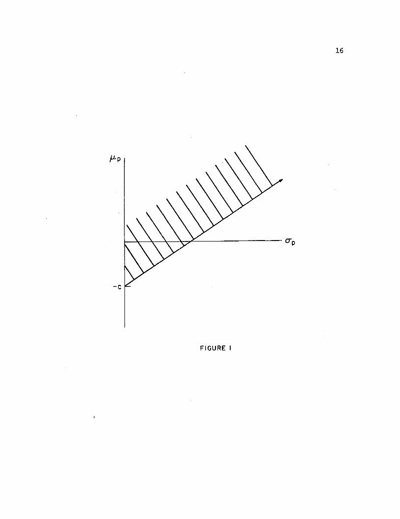
16

- C

FIGURE I

I

17vi ( i + avi / aL. . L;L/ v i )

+X2 (ayp/3Li + 2(a)aop/3Li ) = ^ (7)

where, by definition, Xa is the change in market value realized from a change in loanable funds,16 3H/3K , and optimality between any two loans is defined in terms of the safety-first constant. Credit extension, therefore, occurs up to the point where, for any two loans, i,j, the marginal revenue generated from the loan is exactly offset by the increased probability of default.17 Explicitly, this relationship is shown by:

3H/3C = X2 = Vi ( ( l +3V./aLi -Li / V. )

- V.(1 + 3V . /3L. »L. / V. ) ) / /aL.3 3 3 3 3 P i+Z(a)3o /3L.-3y / 3L.+2(a)3a /3L. (8)P P 1 P I

16 where H is the Lagrangian expression of (6), H = N

N N+ X1 (K-Z L.) +X2 (yp + Z (a) ap + C) + Z 2T.L.

17 The increase in the market value of the bank as a result of increased risk in the credit portfolio should be compared to the increase in expected costs of bankruptcy. Swary assumes that a and the safety-first constraint are determined in a way that reflects these considerations.

18The Financing Decision

In order for the bank to complete the list of decision variables contained in Swary's model, it must evaluate the liabilities markets and select that debt-equity mix which will optimize market value. The market for the bank's liabilities include deposits, purchased funds and equity capital. Each source of funds provides the bank with necessary cash inflows and a unique pricing structure.

DepositsDeposits provide customers with a two-dimensional

product, one that satisfies the customer's demand for transaction services and acts as an investment for depositors. Thus, the actual investment in deposits is assumed to be a function of the differential between yields on similar risk assets, the explicit transfer cost, and the inelastic demand for deposits as a transactions vehicle. Therefore, deposit levels are assumed to be exogenous to the decisions of the commercial bank.

Purchased FundsPurchased funds represent a dynamic medium for banks to

obtain sources of funds. Since the 1960's, purchased funds (large negotiable certificates of deposit, federal funds, Eurodollar loans and Federal Reserve loans) have represented

19a large reservoir of funds .which are traded in a highly competitive market and provide the banking system with necessary liquidity. In general, purchased funds are assumed to be homogenous with respect to maturity, rates, reserve requirements and increasing marginal acquisition costs, and are the banks only source of debt funds in this model.

gggitgSupplies of equity capital are assumed to flow from an

efficient market providing no consistent abnormal (risk-adjusted) returns. Equity acquisition costs are positive and are assumed to exceed that of purchased funds. In contrast, they are inversely related to issue size.

Financing Decision: Selecting the Optimal Capital Structure

Assumptions:To introduce the relevant capital markets into the

financing model, Swary makes the following additional assumptions:

1. Loans are considered homogenous in a risk-return sense with a perfectly elastic supply. The loans purchased, determined at the beginning of a one-period planning horizon, carry fixed rates.

2. A negative covariance exists between deposit inflows and the yield on money market funds.

3. Money market rates exhibit high degrees of variability with low transaction cost on a volume basis and increasing marginal borrowing costs.

204. The level of equity capital is assumed constant

throughout the period. Thus deposit fluctuations are met with purchased funds.

The notation is similar to that of the previous equations,with:r = interest factor on loans.V = returns from information per dollar of loan (note the

subscript is dropped due to homogeneity of loans).= deposit yielding zero interest, t=0,l.

In addition, define:i0 = the stochastic public deposit flow during period 1,

bounded by -D0 and Dj, , the upper bound on maximum deposit inflow during the period.

i = rate paid for purchased fundscov(11,i ) = covariance between deposit inflows and

rate paid on purchased funds.3(F) = relative change in i as a function of

acquisition of purchased funds.T(F) = transactions costs associated with debt funds,

T 1(F )>0, T ' '(F)>0.T(C) = transaction cost associated with equity funds

T'(C)>0, T''(C)<0. Where by assumption T(C) > T(F).

The bank's decision now becomes one of choosing the optimal amount of loans and borrowed (purchased funds and equity) funds which would result in maximizing the market value of the firm:

MAXIMIZE (MV-C) = LV-T(C)-T(F) / (F-T)f(x)dT (9)

-D0subject to:

21Ft+Dt+C = L

V +Z(a)o = -C P P

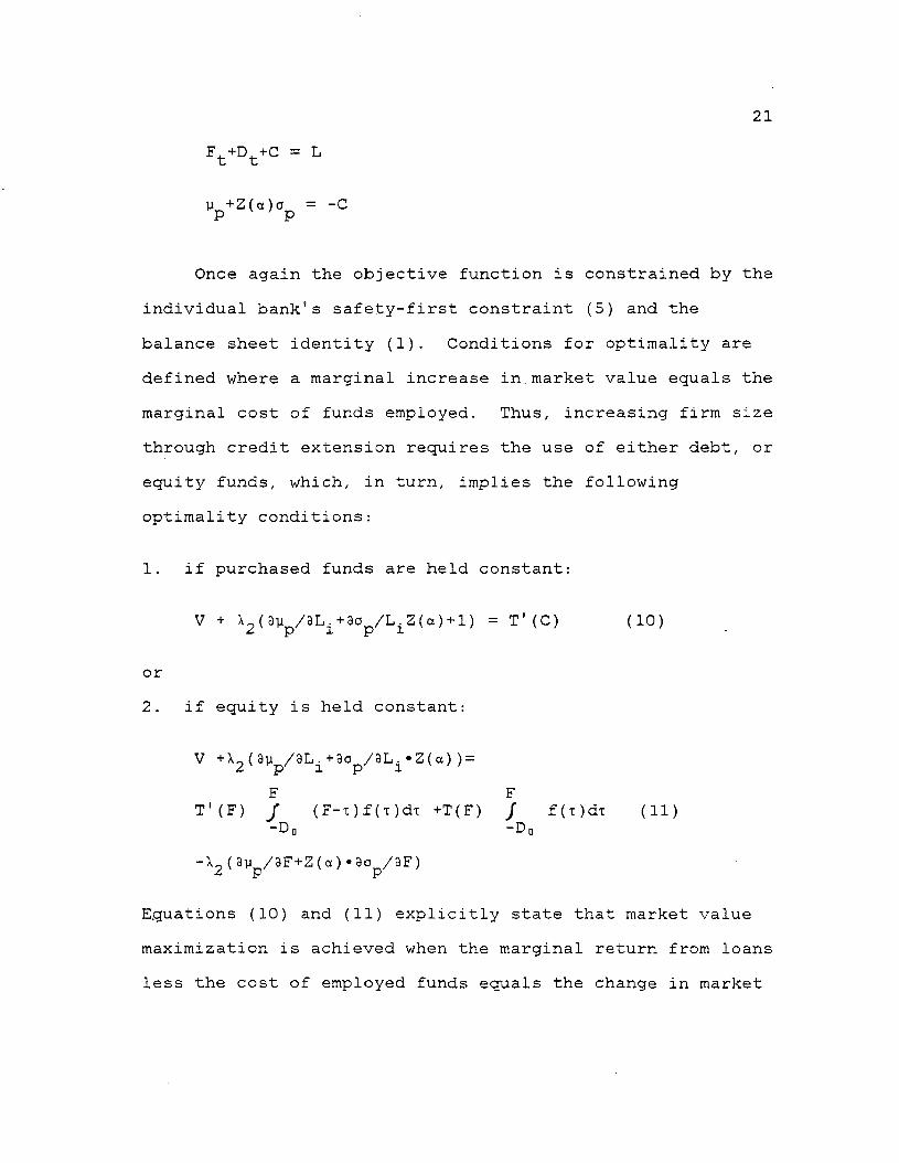
Once again the objective function is constrained by the individual bank's safety-first constraint (5) and the balance sheet identity (1). Conditions for optimality are defined where a marginal increase in.market value equals the marginal cost of funds employed. Thus, increasing firm size through credit extension requires the use of either debt, or equity funds, which, in turn, implies the following optimality conditions:

1. if purchased funds are held constant:

V + X2 (3yp/aLi+3op/LiZ(a)+l) = T'(C) (10)

or2. if equity is held constant:

V +X2 (3yp/3Li + 3op/3Li»Z(a) ) =F F

T'(F) J (F-x)f (t)dt +T(F) / f(t)di (11)-D g -D 0

-X2 (3yp/3F+Z(a).3op/3F)

Equations (10) and (11) explicitly state that market value maximization is achieved when the marginal return from loans less the cost of employed funds equals the change in market

22value resulting from a change in the probability of bankruptcy.

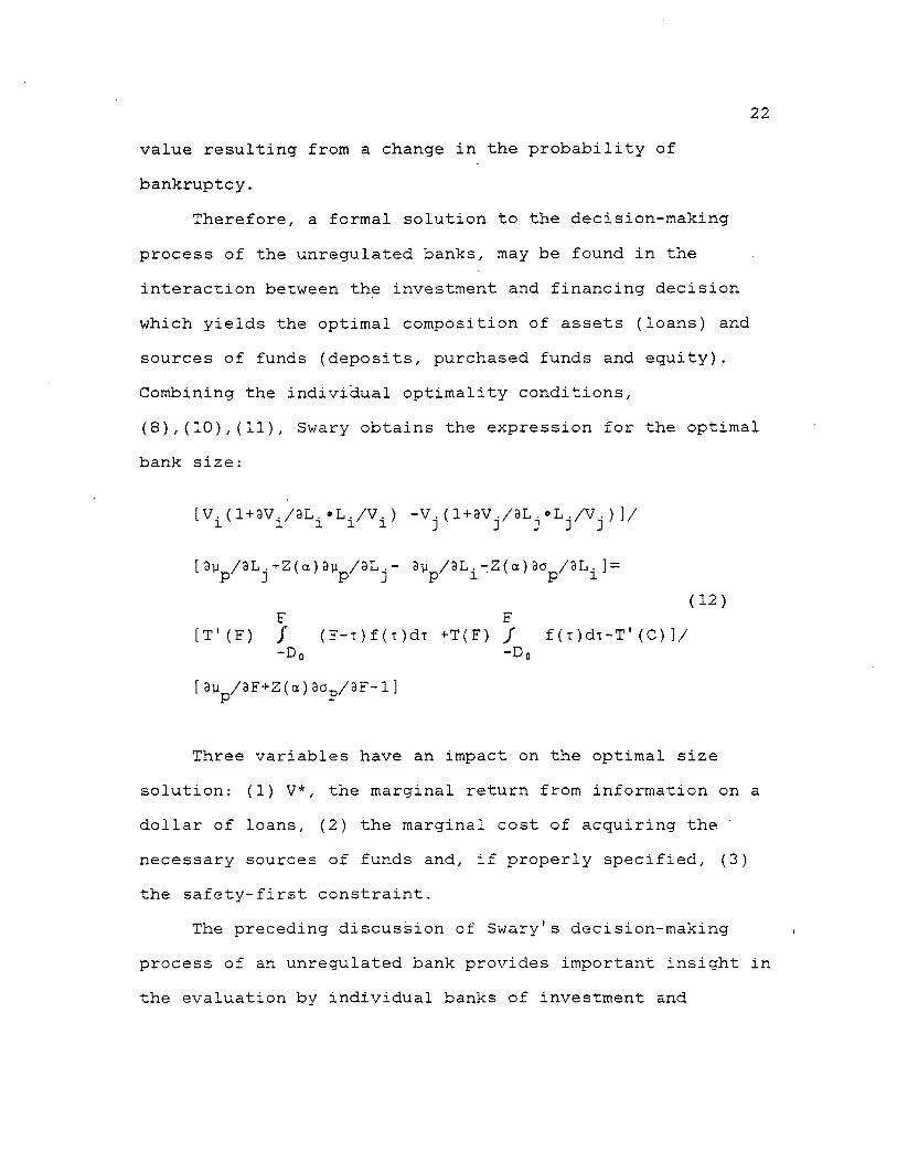
Therefore, a formal solution to the decision-making process of the unregulated banks, may be found in the interaction between the investment and financing decision which yields the optimal composition of assets (loans) and sources of funds (deposits, purchased funds and equity). Combining the individual optimality conditions,(8),(10),(11), Swary obtains the expression for the optimal bank size:

[Vi(l+3V./9Li.Li/Vi ) -Vj(l+3Vj/3Lj.Lj/Vj )]/

[ 3iip/3Lj+Z(a)3Rp/3Lj- 3y /SL^-Z(a ) 3ap /3L. ] =

(12)F F

[T '(F ) / (F-T)f(T)dt +T(F) / f(x)dT-T'(C)]/-Do -Dq

[3p /3F+Z(a )3o_/3F-1]

Three variables have an impact on the optimal size solution: (1) V*, the marginal return from information on adollar of loans, (2) the marginal cost of acquiring the necessary sources of funds and, if properly specified, (3) the safety-first constraint.

The preceding discussion of Swary's decision-making process of an unregulated bank provides important insight in the evaluation by individual banks of investment and

23financing opportunities, and also provides a framework through which the effect of regulation can be measured.

Banks Decision Making Process Under RegulationIn order to measure the effect of regulation on a

commercial bank's decision-making process, Swary introduces various constraints into his unregulated model to serve as proxies for different forms of regulation. This type of analysis supplies descriptive insight into the bank decision-making process and highlights the deficiencies of regulation from a normative viewpoint.

Swary employs a direct chance constraint to estimate the normative comparative statics. These estimates are in turn contrasted with the statics from various portfolio contraints intended to serve as real world proxies of capital regulation. Equally important is how the normative versus the descriptive cases differ and what reaction banks may have in response to regulation. In all cases, the effect of regulation is measured in terms of default risk via return variance.

24Normative Case:Direct Chance Constraint

In order to apply the direct chance constraint to the normative model, it is assumed that regulators can, in fact, determine the upper bound on the probability of failure which is acceptable and enforceable. This means that the regulatory agency must set a limit on failure, which is somehow introduced into the unregulated model. Summarizing Swary's model under this normative direct chance constraint, it is found that, as the constrained probability of failure decreases,

1. the level of equity increases, reducing the reliance on financial leverage.

2. the value of an additional dollar of loans decreases, 3X1/3Z(a)<0 .(See footnote 16).

3. the shadow price of the safety-first constraint increases,3X2/3Z(a) >0 .(See footnote 16).

This third result reinforces the actual interrelationship between the investment and financing decisions as implied by the optimality requirement of higher returns for a given loan and lower financial leverage with respect to the unregulated bank. This result is not surprising, considering the intent of regulation is to improve the soundness of the banking industry and each of these conditions provides a reduction in the probability of failure.

25Descriptive Model--Capital Regulation

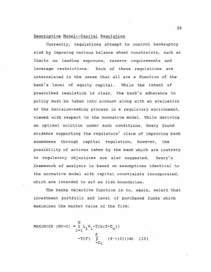
Currently, regulations attempt to control bankruptcy risk by imposing various balance sheet constraints, such as limits on lending exposure, reserve requirements and leverage restrictions. Each of these regulations are interrelated in the sense that all are a function of the bank's level of equity capital. While the intent of prescribed regulation is clear, the bank's adherence to policy must be taken into account along with an evaluation of the decision-making process in a regulatory environment, viewed with respect to the normative model. While deriving an optimal solution under such conditions, Swary found evidence supporting the regulators' claim of improving bank soundness through capital regulation; however, the possibility of actions taken by the bank which are contrary to regulatory objectives are also suggested. Swary's framework of analysis is based on assumptions identical to the normative model with capital constraints incorporated, which are intended to act as risk boundaries.

The banks objective function is to, again, select that investment portfolio and level of purchased funds which maximizes the market value of the firm:

NMAXIMIZE fMV-Cj = E L.V.-T(b(F+D ))i=l 1 1 °

F-T(F) / (F-x)f(t)dt (13)

-D0

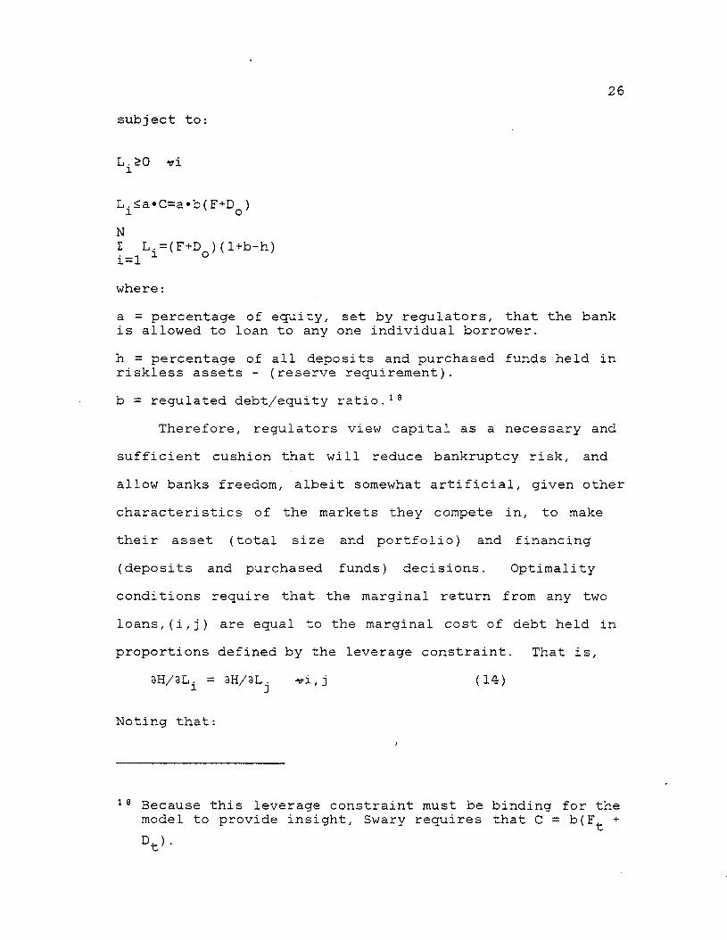
26subject to:

L .>0 vi 1

L .<a«C=a»b(F+D ) i ' o 'N1 L .=(F+D )(1+b-h)• _i i oi = lwhere:a = percentage of equity, set by regulators, that the bank is allowed to loan to any one individual borrower.h = percentage of all deposits and purchased funds held in riskless assets - (reserve requirement).b = regulated debt/equity ratio.18

Therefore, regulators view capital as a necessary andsufficient cushion that will reduce bankruptcy risk, andallow banks freedom, albeit somewhat artificial, given othercharacteristics of the markets they compete in, to maketheir asset (total size and portfolio) and financing(deposits and purchased funds) decisions. Optimalityconditions require that the marginal return from any twoloans,(i,j) are equal to the marginal cost of debt held inproportions defined by the leverage constraint. That is,

3H/3Li = 3H/3L^ * i ,j (14)

Noting that:

18 Because this leverage constraint must be binding for the model to provide insight, Swary requires that C = b(F^ +

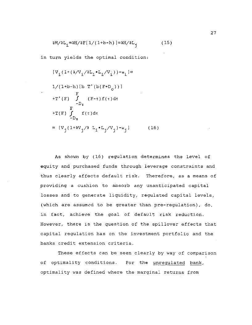
273H/3Li = aH/aF[ l/( 1+b-h) ]=3H/3Lj (15)

in turn yields the optimal condition:

[V.(l+(3/V±/3Li-Li/Vi ))-«i ]=

1/(1+b-h)[b T'(b(F+D ))]F

+T'(F) / ( F-t )f (t )dx-D0F

+T(F) / f(t)di “Do

= [V.(l + 3V./3 L . • L ./V .)-<*>•] (16)i y i y i i v '

As shown by (15) regulation determines the level of equity and purchased funds through leverage constraints and thus clearly affects default risk. Therefore, as a means of providing a cushion to absorb any unanticipated capital losses and to generate liquidity, regulated capital levels, (which are assumed to be greater than pre-regulation), do, in fact, achieve the goal of default risk reduction. However, there is the question of the spillover effects that capital regulation has on the investment portfolio and the banks credit extension criteria.

These effects can be seen clearly by way of comparison of optimality conditions. For the unregulated bank, optimality was defined where the marginal returns from

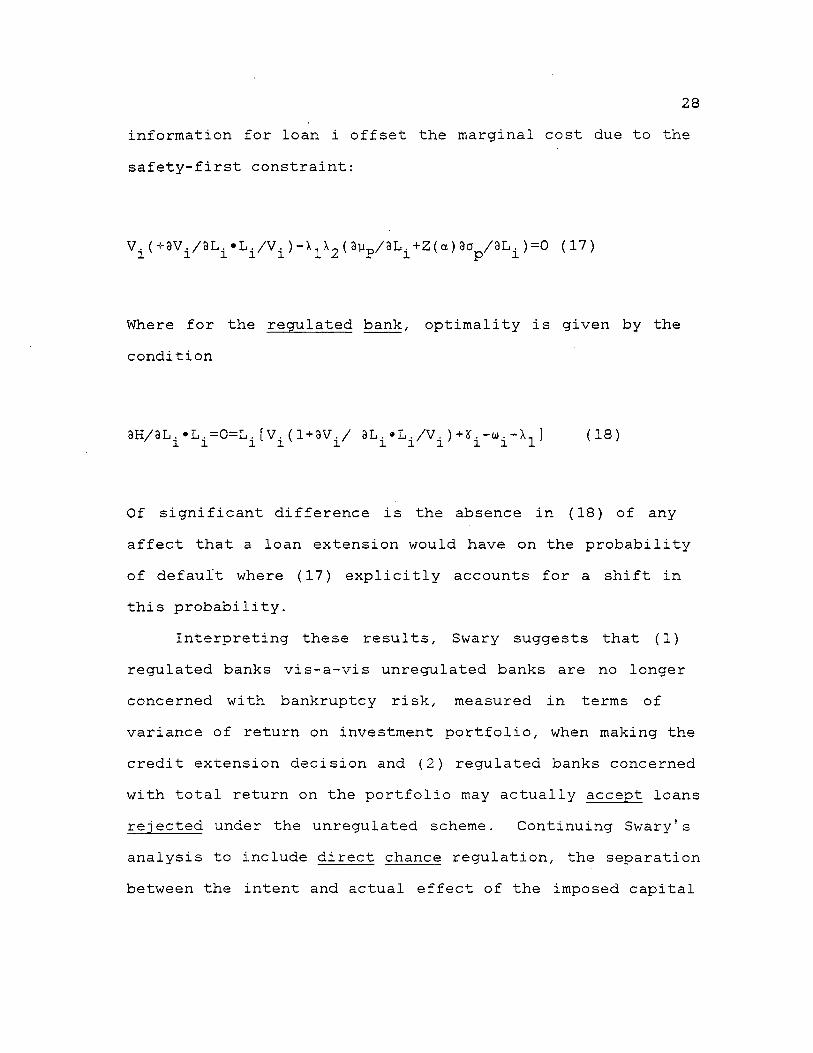
28information for loan i offset the marginal cost due to the safety-first constraint:

V i(+3Vi/aLi*Li/Vi )-X1X2 (3Vp/3Li+Z(a)3op/aLi )=0 (17)

Where for the regulated bank, optimality is given by the condition

3H/3L.•L.=0=L.[V.(1+3V./ 3L.•L ./ V .)+Z.-u.-\.] (18)/ 1 1 1 l' l H / l ' l l l v /

Of significant difference is the absence in (18) of any affect that a loan extension would have on the probability of default where (17) explicitly accounts for a shift in this probability.

Interpreting these results, Swary suggests that (1) regulated banks vis-a-vis unregulated banks are no longer concerned with bankruptcy risk, measured in terms of variance of return on investment portfolio, when making the credit extension decision and (2) regulated banks concerned with total return on the portfolio may actually accept loans rejected under the unregulated scheme. Continuing Swary's analysis to include direct chance regulation, the separation between the intent and actual effect of the imposed capital

29regulation becomes apparent/ Here again Swary notes the bank's disregard for portfolio risk in the investment decision. "Where as the intended effect of regulatory constraints is to decrease the rate of substitution between risk and return in all decisions, including investments(loan exstension), such constraints eliminate any risk considerations which are liable to increase the variance-risk of a loan portfolio."19

Bank Reaction to Capital RegulationSwary's conclusions appear to indict the overall

effectiveness of capital regulation with respect to the bank's decision making process. But his model falls short of a rigorous evaluation of the hypothesis that banks do indeed take on more risky (variance-risk) portfolios as a result of capital regulation. Such an evaluation requires a re-evaluation of the investment decision and any possible limitations the capital (leverage) constraint would impose. It must be noted, however, that the problem does not arise due to the inadequacy of regulation, but as a result of the reaction by the decision-makers, post-regulation. In an independent study Koehn and Santomero (1980), here after denoted K-S, identify the dilemma caused by regulation and

t

provide a model that explicitly examines this reshuffling

19 Swary (1980), pg. 49.

30hypothesis. Their framework-of analysis recognizes that the intent of regulation is to reduce default risk of banks, but assuming that portfolio risk is not adequately constrained by regulation, the hypothesized reshuffling is indeed plausible.

Koehn-Santomero Portfolio Investment Model

Assumptions1. The total assets size is a decision variable of bank

management. In the sense that only amounts of debt relative to equity is regulated, bank size is unconstrained.

2. The rate paid on the negative asset (deposits) is risk free but a riskless asset (positive-holding) is not available.20

3. In constrast to Swary, K-S model the banks as asingle-period risk averse expected utilitymaximizer.21

4. Whichever risk-averse function is chosen, it isassumed to be approximated by a Taylor-series expansion truncated after the second moment.

5. While not necessary to the derivation, the bank is assumed to operate in a competitive market. "Given that the regulator fixes the capital to assets ratio K = E/TA, the choice problem facing the bank is to determine (1) its optimal scale, i.e., the amounts of both deposits and equity to issue, and (2) the optimal allocation of this asset pool over the

20 Essentially the bank issues the risk free asset in the Koehn and Santomero model.

21 This assumption agrees with the work done by Michealsen and Goshay (1967) and is intuitively appealing considering that the majority of banks are, in fact, closely held.

31available risky asset set."22 In essence, the regulators view financial leverage as being detrimental to financial soundness and thereby use capital regulations to retard the bank's use of financial leverage. Since size is assumed to be a choice variable (assumption 1) and the market is assumed to be a competitive one,23 the bank may increase its use of financial leverage only by increasing capital and size and it may lever itself (and of course its earnings) without limit. Therefore the allocation process becomes paramount to the bank and, as given by assumption 4, will be described in terms of risk/return (variance) per unit of equity capital.

Theoretically, the bank must determine, out of the universe of risky assets, which assets to purchase, and the weightings of such assets that maximize its utility function. Applying the formulation suggested by Merton (1972), K-S describe the banks portfolio decision as the following:

N NMINIMIZE 1/2 Z Z x.x.o. .-X E(R ) (19)/i=1j_1 i 3 i/J o p'

Subject toN

(20)

x q£ 1-1/K (21 )N

E (R )=x R- + Z x .E (R .) (22)' p y o f . l v l ' v 'i = l

22 Koehn and Santomero (1980), pg. 1236.23 For a discussion of the implications of imperfect

competition refer to James (1976).

32where:E(R^) = expected return on ith asset.

= percent of equity value invested in the ith asset.a. . = covariance between asset i and j. ijE(Rp),0p 2 = expected portfolio return and

variance/unit of equity.Xq = percent of equity held in deposits paying risk free returnR̂ . = risk free rate of return.X = trade-off between risk,a 2, o P

and return E(R^) at any point on the efficient frontier.K = Equity Capital/Total Assets.

While the regulator attempts to set an upper limit on leverage, as seen through the inequality in (21), the major thrust of the analysis is the effect of such regulation on the decision making process of the bank. Therefore, in order to model the bank's reaction the capital constraint,(21) must be binding:

x q = 1-1/K (21.1)

The necessary conditions for determining the optimal investment portfolio chosen by the bank, given the capital constraint, are 1) the simultaneous solution to (19) through(22) and 2) the condition set fort by X0,i.e., the marginal rate of substitution as exhibited by the firm's objective function.

33The Individual Banks Utility Function

In order to equate X0 with the marginal rate of substitution, first assume that the bank possesses a single period risk-averse utility function expressed in terms of end-of-period capital:

U = U(C + RpC) (23)

Expanding this function around beginning capital yields:

U = U(C) + U'(C)RpC + U''(C)(RpC)+ higher order terms (23.1)

The expectation of (23.1) becomes:

E(U) = E[U(C)] + U'(C)CE(R )r*

+ 1/2U''(C )C 2E (R 2) (24)P

Now define o 2 as:P

E (Rp-E(Rp ))2 = E(Rp 2)-[E(Rp )]2 (24.1)

and substituting (24.1) into (24) yields:

E(U) = EtU(C)] + CU'(C)•[E(R )+U" (C)/2U! (C)»C*{E(R )2+c 2 } ] (25)

lr r

As formulated by Pratt (1964), an estimate of the relative risk aversion exhibited by a particular utility function is in general given by:

34U ' '(C)C

RRA (26)2U1(C)

The utility function adopted by K-S is defined to be functionally related to end-of-period capital, with a relative risk aversion coefficient given by:

U 1'(C)Cr = - _________________ (27)

2 U'(C)

Introducing r into (25) enables expected utility to beexpressed as a function of E(R ),o 2 and r.P P

E(U) = U(C)+ U' (C)C[E(Rp )-r[E(Rp )2+op 2H (28)

Now, the second necessary condition to obtain an optimal solution to (19) can be achieved by deriving an expression for the marginal rate of substitution between risk and return, and, in turn, equating this to \Q . Thusdefine:

MRS . 2o 2,E(R ) P P ; do 2 P

dE<V U=U

351/r-2E(Rp ) (29)

and equating to \q obtains:

X = MRS 2 , = l/r-2E(R ) (30)o °p /E (Rp) 7 p'

Substituting (30) into (19)-(22) K-S derive the desiredinvestment allocation value, Xi*, i.e., the optimal weightof asset i held in the portfolio. Specifically:

Xi* = A»C(l/r-2Rf)-C(1+B)1/KN N

•ll (E(R )-R (^ ))/A- (AZ rp . /C ) ]j=l 3 3 i=l 3N

+ [Z (E(R )-R )/A-l/K] (31)3=1 3 3

where:24 N N

A=Z Z rp..(E(R,)-Rf)i=lj=l 13 3N N

B=Z Z rp. . (E(R. )-R.) (E(R.)-R-)i=lj=l 1 f J fN N

C=Z Z rp. .• -1 nill=lj=l JD = BC-A2

24 rp _ are the elements of the inverse of the variance covariance matrix, i.e.,21 = (^— ), see Merton ( 1972 ).

36The Reaction of Bank to Capital Regulation

We now begin to see how capital regulation affects theinvestment decision of the bank, inasmuch as the optimalinvestment proportion in risky asset i per unit of capitalis shown to be a function of the return generating functionof the available assets, the individual bank's relative riskaversion parameter and the capital ratio. In fact, theimpact of capital regulation becomes transparent when viewedin light of the marginal effect on the decision makingprocess as a result of a change in K, the capitalconstraint. Given the circumstances at hand, K-S25 suggestthe following:26

From the budget constraint (21) and the capital constraint (22), it is clear that the bank will be unable to leverage its capital to the degree it had prior to an increase in K, and moreover, because of the new more stringent restriction on the leverage capability of the bank, the banks efficient investment frontier falls downward and to the left for any given level of capital., i.e.,

25 Koehn and Santomero (1980), pg. 1239.26 See Koehn (1979) for detailed discussion of the effects

of various restrictions on the efficient frontier.

3E (R ) P<0 (32)

3K 3K

' 37Equation (32) therefore provides support for capitalregulation as the post-regulation investment opportunitiesof the bank possess less risk in terms of a 2 , for everyPpossible portfolio return. The central question remains, however, what will be the reaction of the bank in response to the proposed capital regulation?

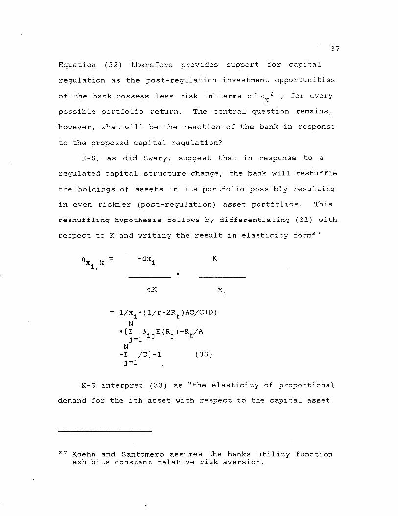
K-S, as did Swary, suggest that in response to a regulated capital structure change, the bank will reshuffle the holdings of assets in its portfolio possibly resulting in even riskier (post-regulation) asset portfolios. This reshuffling hypothesis follows by differentiating (31) with respect to K and writing the result in elasticity form27

dK x.l

= l/xj.* (l/r-2Rf )AC/C+D)N

• [ I <p . . E (R . ) -R^/A j=l i] V 3 fN-I /C]-l (33)j=l

K-S interpret (33) as "the elasticity of proportional demand for the ith asset with respect to the capital asset

27 Koehn and Santomero assumes the banks utility function exhibits constant relative risk aversion.

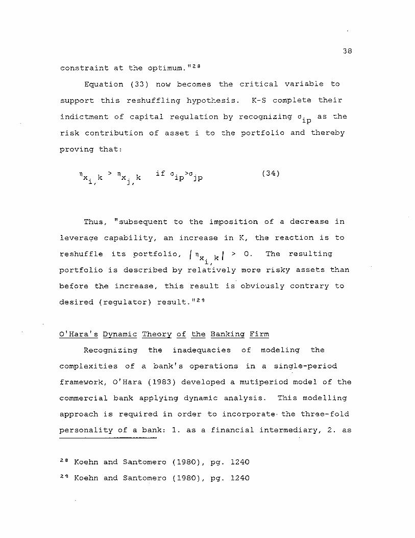
38constraint at the optimum."28

Equation (33) now becomes the critical variable to support this reshuffling hypothesis. K-S complete their indictment of capital regulation by recognizing a. as the

trrisk contribution of asset i to the portfolio and thereby proving that:

ti 1 >ti , if o. >o. (34)x. k x. k ip ip ' 'i, J, *

Thus, "subsequent to the imposition of a decrease in leverage capability, an increase in K, the reaction is to reshuffle its portfolio, j ri kl > ^' result;i-n9

i ,portfolio is described by relatively more risky assets than before the increase, this result is obviously contrary to desired (regulator) result."29

0 1Hara1s Dynamic Theory of the Banking FirmRecognizing the inadequacies of modeling the

complexities of a bank's operations in a single-period framework, O'Hara (1983) developed a mutiperiod model of the commercial bank applying dynamic analysis. This modelling approach is required in order to incorporate- the three-fold personality of a bank: 1. as a financial intermediary, 2. as

28 Koehn and Santomero (1980), pg. 124029 Koehn and Santomero (1980), pg. 1240

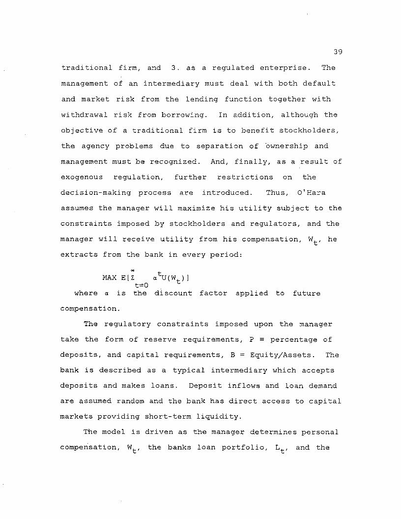
traditional firm, and 3. as a regulated enterprise. The management of an intermediary must deal with both default and market risk from the lending function together with withdrawal risk from borrowing. In addition, although the objective of a traditional firm is to benefit stockholders, the agency problems due to separation of ownership and management must be recognized. And, finally, as a result of exogenous regulation, further restrictions on the decision-making process are introduced. Thus, O'Hara assumes the manager will maximize his utility subject to the constraints imposed by stockholders and regulators, and the manager will receive utility from his compensation, W^, he extracts from the bank in every period:

00 tMAX E [ I o U(W ) ]t=0 r

where a is the discount factor applied to future compensation.

The regulatory constraints imposed upon the manager take the form of reserve requirements, P = percentage of deposits, and capital requirements, B = Equity/Assets. The bank is described as a typical intermediary which accepts deposits and makes loans. Deposit inflows and loan demand are assumed random and the bank has direct access to capital markets providing short-term liquidity.

The model is driven as the manager determines personal compensation, Wfc, the banks loan portfolio, L^, and the

40level of deposit services, S^, at the beginning of period t. The deposit services generate deposits for period t, D̂ ., and loans granted are due at the end of the period. At the end of period t, bank profits are determined, stockholders receive dividends and period t+l's net worth is known, Y. Bankruptcy is defined where net worth at the end of the period is below that level required by regulators, Y < B. If Y > B then the manager has satisfied both stockholders and regulators and the bank's operations continue.

Of interest to this study is how the manager's decision-making process may be altered by changes in the net worth constraint. As pointed out by Koehn and Santomero, one effect of a change in capital regulations is a reduction of feasible or permissable investments by the manager. In turn, this altering of the investment opportunity set will result in a reduction of the managers present value of wealth, if his investment portfolio remains unchanged. O'Hara examines the reaction by the manager as a result of capital regulation and concludes that if the manager percieves that the future operations of the bank cannot sustain the new required net worth level, it may be optimal for the manager to take the money and run.30 Another possibility, however, is that the manager invests in a riskier portfolio in the hopes that the higher mean return

30 O'Hara (1983), p.139.

41on such investments can produce a higher profit level for the bank. Of course the irony is, as recognized by others, that this paradoxical situation that increasing the required net worth to presumably make the bank safer results in an increased risk exposure for the bank.

Summary

- Based on the regulators intent that capital regulation improves, reduces risk, the soundness of the banking firm, three model's have been discussed in hopes of evaluating the impact of this form of regulation.

Swary's model of the unregulated bank was examined to serve as a benchmark from which to judge capital regulation's effect on the decision-making process. Under this unconstrained (exogenous) environment, the banks' optimal investment and financial decision was found by equating the information resulting from the marginal dollar of investment (loan, investment securities, etc.) and the marginal cost of funds with respect to the individual bank's safety-first constraint.

Further, it was seen that by introducing capital regulation, risk was expected to be lower, as illustrated by

lSwary's normative model. But, it was revealed, in a practical sense banks may ignore the effect that various

investment and financing decisions have upon their riskiness. In particular, when Swary introduced the capital-asset ratio , optimality conditions equated marginal revenue of investments with marginal financing costs, but the absence of a default risk variable in the optimal solution suggested possible deficiencies in capital regulation. And, as suggested by Swary and rigorously derived by Koehn and Santomero and O'Hara, banks, as a result of capital regulation, may actually reshuffle their asset portfolio, resulting in a more risky post-regulation asset portfolio. Such a result, therefore, suggests that not only is capital regulation ineffectual, but possibly detrimental to the underlying riskiness of the banking industry.

Chapter III CAPITAL REGULATION AND BANKRUPTCY RISK

IntroductionThe analysis thus far suggests two propositions

regarding the effects of capital regulation:1. In response to a regulated shift in capital

structure, the bank attempts to offset the reduction in financial leverage by reshuffling its asset portfolio, resulting in a more risky position.

2. As a result of such reshuffling the post-regulation probability of bankruptcy may differ from regulatory intent and, in particular, may increase.

Justification for proposition 1 stems from the forementioned models of Swary and Koehn-Santomero. Further discussion of this point will be reserved for a later chapter in as much as we will attempt to empirically test this reshuffling proposition.

Keeping in mind that regulators employ various regulations in order to control the soundness of the banking industry, i.e., entry restrictions, pricing constraints, activity restrictions, capital structure control and insider abuse restrictions,31 discussion of proposition 2 is necessary to evaluate the implications the reshuffling

31 For a detailed discussion of these regulations see Edwards and Scott (1978).

43

44hypothesis has upon bankruptcy risk.

So far, except for a few comments of the Swary model, a theoretical link between the intent of specific regulation and bankruptcy risk is noticeably absent.

Scott-Edwards Bankruptcy ModelA rather elegant approach to modelling bankruptcy risk

for the commercial bank was suggested by James Scott and Franklin Edwards (1977). The Scott-Edwards analysis was done in a framework of how two hypothetical banks are affected by soundness regulations. These two banks are primarily differentiated by their access to capital markets:

1. The partial access bank (PAB) is assumed to haverestricted access to capital markets in the sense that information costs are higher for these banks (smaller in total assets) resulting in inefficiencies in the pricing of their securities. This assumed restricted access in effect requires that partial access (smaller banks) banks rely heavily on the sale of assets in raising needed funds.

2. The full access bank (FAB) is characterized by theability to raise funds in both debt or equity markets and that their security issues are fairly priced.

45Using a traditional measure of bankruptcy, as the point

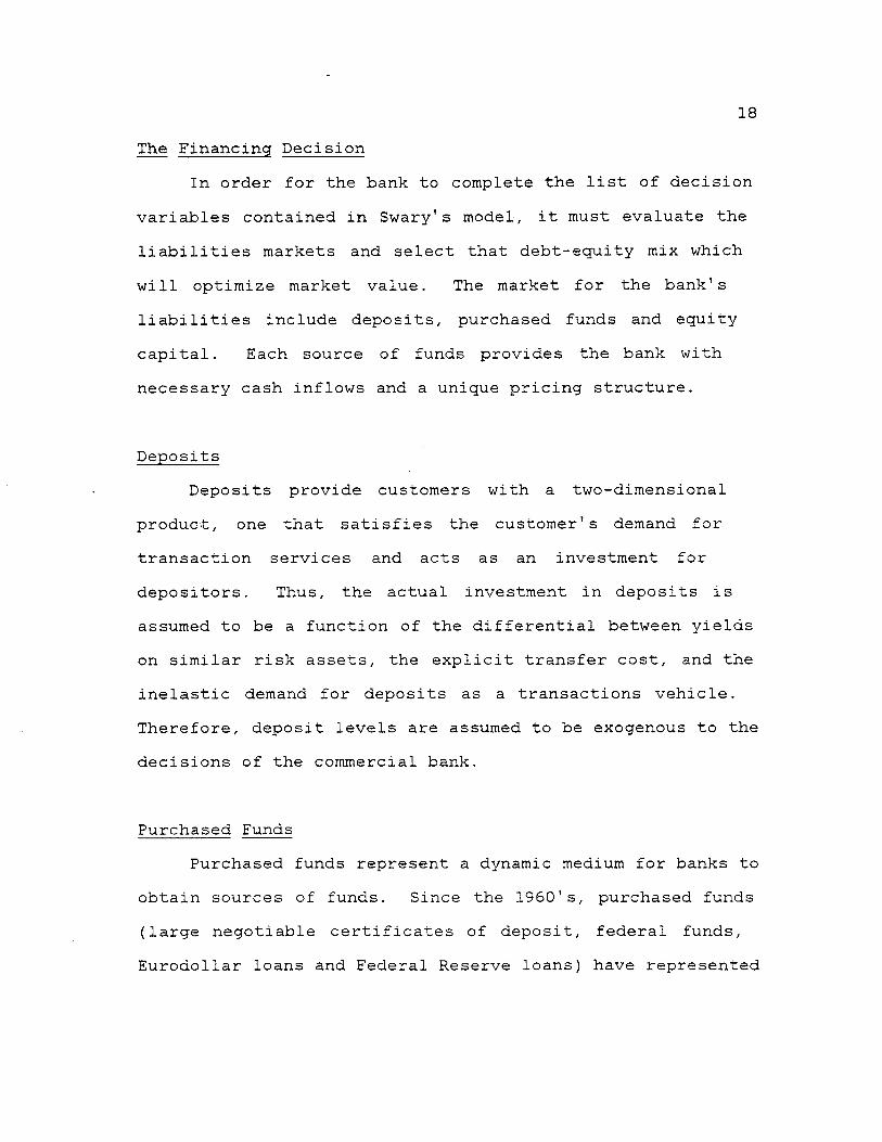
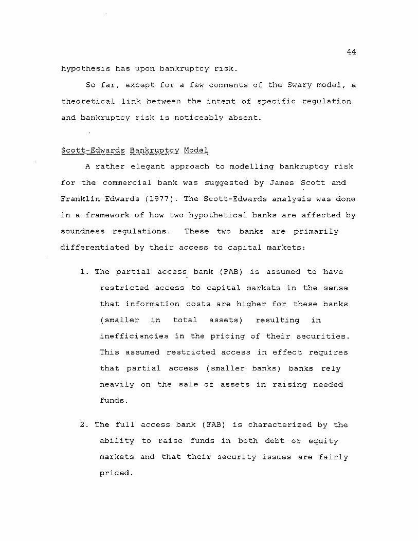
where cash flows of the bank from operations, X, fall below some critical level b in a mean standard deviation framework, it is obvious that given a change in either parameter of the distribution of cash flows yields a corresponding change default probability. Graphically, the probability of bankruptcy,(Pr X < b) is shown in Figure 2. Thus, it is apparent that bankruptcy (insolvency) is achieved when either operating losses, devaluation of assets or large withdrawal of funds (deposits) results in insufficient cash as to meet its current obligations. Based on their respective definitions, the partial access bank more closely parallels the banks included in the forthcoming empirical analysis, therefore the bankruptcy model will be discussed in terms of the PAB.

X = CASH FLOW BEFORE INTEREST AND TAXES b = PO IN T OF INSOLVENCY

FIGURE 2

(T i

Variable Definitions:

Xi = earnings before interest and taxes plus security gains or losses, EBIT, at period one.

= total assets valued at historical cost, t=0,l

d^ = total deposits

i = interest rate paid on deposit at t=0

= non-deposit bank debt

R̂ _ = interest payments required to service D̂ . ̂ due at t .

T = marginal/average tax rate

In the Scott-Edwards model, the bank is assumed to operate in a two-period world, t=0,l, where period one earnings are assumed random and liabilities are certain.

If cash flows from operations are less than cash needs, the PAB is assumed to sell assets in attempt to remain solvent. Measured at t^, solvency can be defined as the existence of positive net worth, i.e.,

48AA= change in assets from t to t,,AA = A.-A ̂ o 1' 1 o

In addition, the cash flow condition can be seen by defining after-tax cash flow from operations as:

(l-T).(X1-ido-Ro ) (36)

and the net deposit drain as:

(d^-d ) + (D-. -D ) (37)' 1 o ' v 1 o ' v '

For the PAB, the sale of assets will be required to prevent insolvency if (36) plus (37) is less than the critical level b. Further, it is assumed that when the PAB attempts to sell its assets, it faces a decreasing liquidity function receiving ZhKx , from the sale of AAX, where Z < 1. Therefore, as the bank attempts to supplement any operating cash deficiency, the maximum amount of assets at book value that the bank will have to sell is given by:

l/H[(l-T)(X1-id0-R1 )+(d1-d0 ) +(D1-Dq ] = AA1 (38)

which in turn, implies the following solvency condition interms of operating cash flow, Xj,:

X x>[(ido+R1 )-(d1-do )/(l-T>]

-[(D1-Dq )/(1-T)]-[£(A0-d1-D1/(l-T)] (39)

49It is clear that the critical level, b, is equal to the

RHS of (39) and as operating cash flows including the sale of assets, falls below this point, bankruptcy will occur. Referring back to Figure 2, if operating cash flows are assumed to follow a normal distribution characterized by the cumulative distribution function G(X1), then the probability of bankruptcy can be expressed as G(b), the shaded area in Figure 2.

Given this ability to measure bankruptcy probabilities, Scott-Edwards ask the question: For an individual bankpossessing a cash flow distribution as described above, how will changes in the distributions' parameters alter the probability of bankruptcy? Actually, this is the premise underlying the actions of most bank capital regulation and should provide further insight into the evaluation of any proposed constraints.

Parameter Shifts and Bankruptcy ProbabilityUnder the assumption of normally distributed cash flows

three alterations of the parameters are relevant:1. A Change in the mean of the distribution holding

dispersion constant.2. A Change in mean and o . 13. A Change in o.

50Based on the analysis discussed in Scott-Edwards (1977), the effects of such parameter changes on the probability of bankruptcy are presented.

A Change in Mean of the Pistribution of XIn order to see the effects on the probability of

bankruptcy given a change in Xj while holding standard deviation constant, replace X : with X a + a in (39), where a is a "perfectly certain, lump sum, increase (decrease) in before tax earnings."32 (39) then becomes:

X1 > {-ct+b) (40)

where: b equals the RHS of (39);and the probability of bankruptcy for this bank is defined as G (-a + b). The effect of the change in X on G (• ) isseen by taking the partials:

3G( -cc+b)_____________ = -g[-a+b] < 0 (41)

9a

where g (•) = probability density function of X 1(g (• ) = G' (•). Thus the probability of bankruptcy will decline (rise) as a result of increasing (decreasing) mean cash flow.

32 Scott and Edwards (1977), p. 22.

51A Change in Both the Mean and Standard Deviation of X

Such a parameter shift is accomplished by replacing X x with XXj in (39) yielding:

X1 > b/X (42)

where: X>0 andb=RHS (39).

The effect of increasing (decreasing) X increases (decreases) both X and o proportionally and results in a seemingly ambiguous impact on probability of bankruptcy,G (b/X):

3G(b/X) -g[b/\] <__________ = _____________ = 0 (43)

>

ax x2

<

as b = 0

>

Scott-Edwards contend that the most plausible outcome is for b<0, implying that a bank with non-positive earnings before interest and taxes can remain solvent. Under such conditions, an increase in X will unambiguously increase

bankruptcy probability.3352

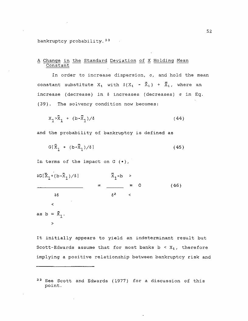
A Change in the Standard Deviation of X Holding Mean ’Constant

In order to increase dispersion, a, and hold the mean constant substitute X x with 6(X: - X a ) + X : , where an increase (decrease) in 5 increases (decreases) a in Eq. (39). The solvency condition now becomes:

X1>X1 + (b-X1 )/5 (44)

and the probability of bankruptcy is defined as

G[X1 + (b-X1)/6] (45)

In terms of the impact on G (•),

3G[X1+(b-X1)/6] j^-b >__________________ = = 0 (45)

36 62 <<

as b = .>

It initially appears to yield an indeterminant result but Scott-Edwards assume that for most banks b < X*, therefore implying a positive relationship between bankruptcy risk and

33 See Scott and Edwards (1977) for a discussion of this point.

53cash flow variability,

3G[ • ]__________ > 0 (47)

36

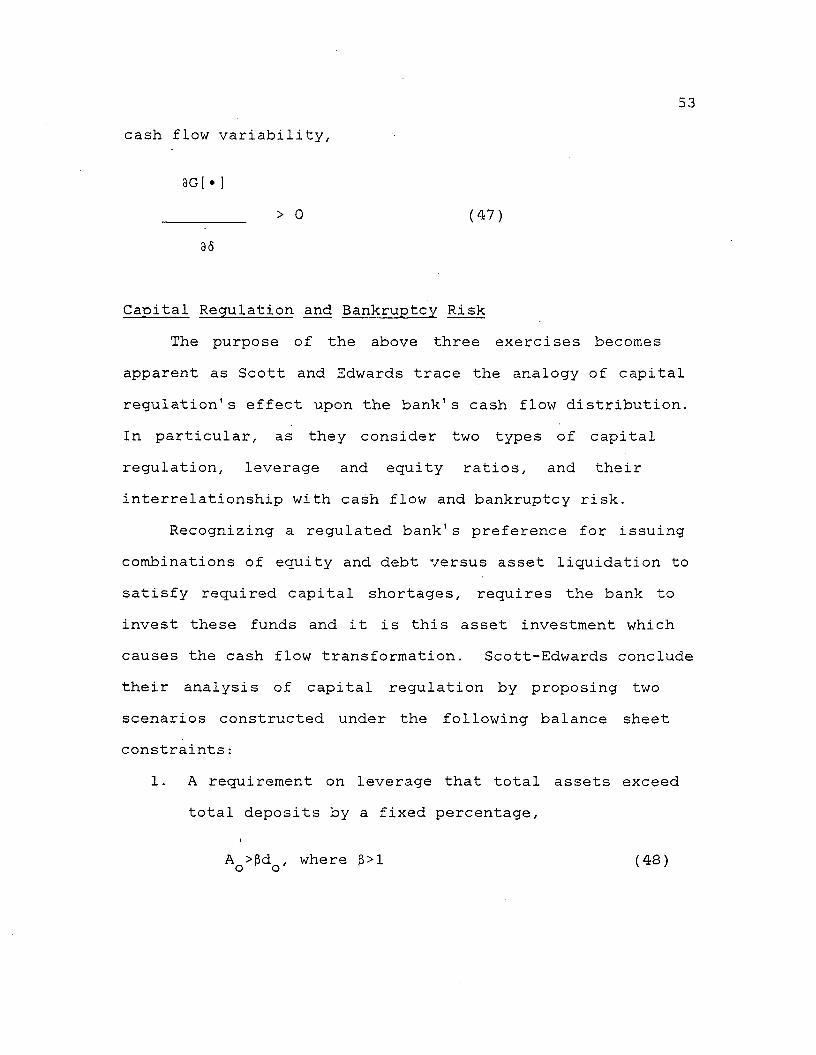
Capital Regulation and Bankruptcy Ri skThe purpose of the above three exercises becomes

apparent as Scott and Edwards trace the analogy of capital regulation's effect upon the bank's cash flow distribution. In particular, as they consider two types of capital regulation, leverage and equity ratios, and their interrelationship with cash flow and bankruptcy risk.

Recognizing a regulated bank's preference for issuing combinations of equity and debt versus asset liquidation to satisfy required capital shortages, requires the bank to invest these funds and it is this asset investment which causes the cash flow transformation. Scott-Edwards conclude their analysis of capital regulation by proposing two scenarios constructed under the following balance sheet constraints:

1. A requirement on leverage that total assets exceed total deposits by a fixed percentage,

lA >(5d , where (3>1 (48)o o

542. A capital ratio of stockholders equity to total

deposits,

A -d -D >0 d , where 0>O (49)o o o o

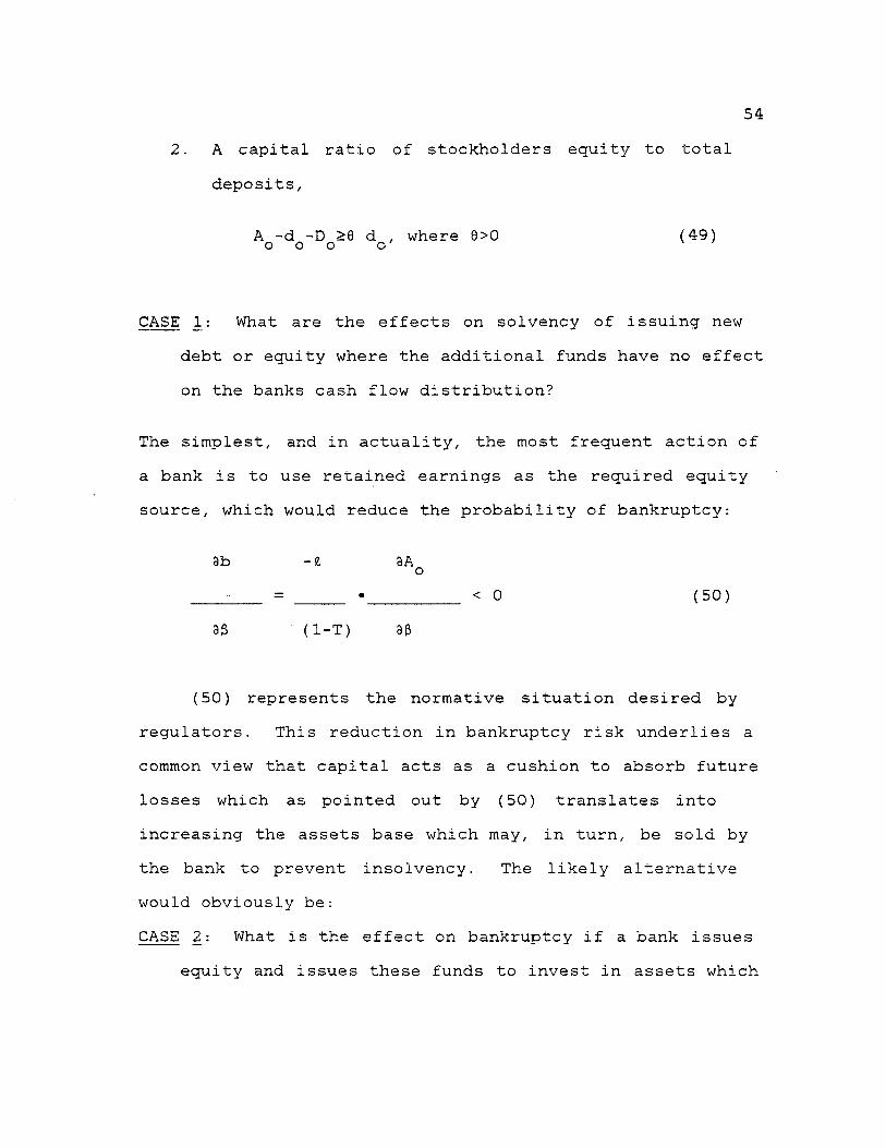
CASE _1: What are the effects on solvency of issuing newdebt or equity where the additional funds have no effect on the banks cash flow distribution?

The simplest, and in actuality, the most frequent action of a bank is to use retained earnings as the required equity source, which would reduce the probability of bankruptcy:

3b -Z 3Ao• = _____ •__________ < 0 (50)

30 (1-T) 30

(50) represents the normative situation desired by regulators. This reduction in bankruptcy risk underlies a common view that capital acts as a cushion to absorb future losses which as pointed out by (50) translates into increasing the assets base which may, in turn, be sold by the bank to prevent insolvency. The likely alternative would obviously be:CASE 2: What is the effect on bankruptcy if a bank issues

equity and issues these funds to invest in assets which

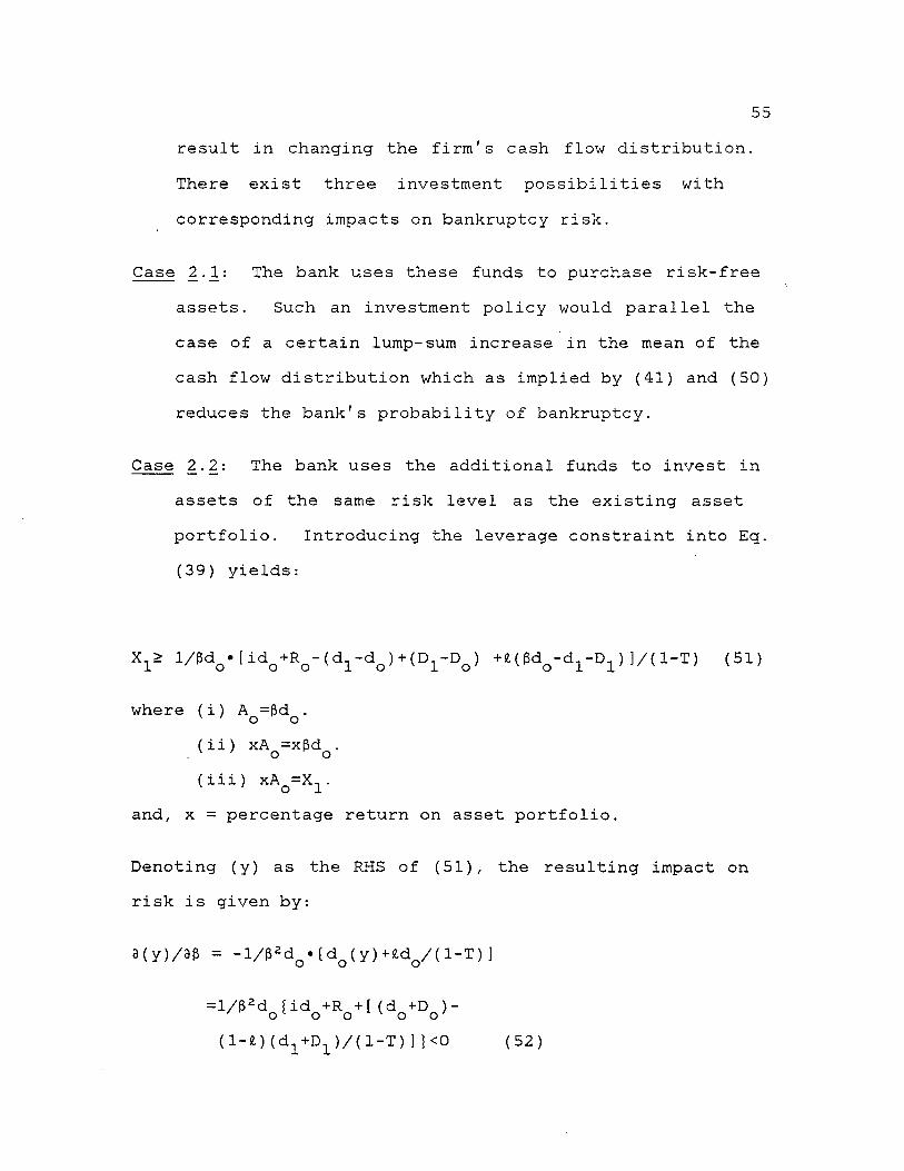
55result in changing the firm's cash flow distribution. There exist three investment possibilities with corresponding impacts on bankruptcy risk.

Case 2.1: The bank uses these funds to purchase risk-freeassets. Such an investment policy would parallel the case of a certain lump-sum increase in the mean of the cash flow distribution which as implied by (41) and (50) reduces the bank's probability of bankruptcy.

Case 2.2: The bank uses the additional funds to invest inassets of the same risk level as the existing asset portfolio. Introducing the leverage constraint into Eq. (39) yields:

X x> l/Pdo.[ido+Ro-(d1-do )+(D1-Do ) +d(Pdo-d1-D1)]/(l-T) (51)

where (i ) A =3d . v ' o o(ii) xA =x£d . . ' o o(iii) xA =X,. x ' o 1

and, x = percentage return on asset portfolio,

Denoting (y) as the RHS of (51), the resulting impact on risk is given by:

a(y)/3& = -l/32dQ «[dQ (y )+£dQ/ (1-T)]

=l/32d [id +R +[ (d +D )- ' o 1 o o v o o'

(1-*)(d1+D1 )/(l-T)]}<0 (52)

56In the case where the bank holds the riskiness of its asset portfolio constant/ as long as d 0 + D 0 > (l-£)(di + D x ) ,then the infusion of equity capital results in a decline in bankruptcy risk.

Case 2.3: Banks issue equity and use the funds to greatlyincrease the riskiness (earnings variability) of its asset portfolio.

Analogous to the effect a proportional shift in the mean and standard deviation of cash flow has upon bankruptcy, it is apparent from (43) and (46) that there exists some risk return locus for the banks portfolio that will increase the probability of failure in spite of increasing the equity cushion. While their model does not explicitly suggest that asset reshuffling will occur they do concur with Swary and cast further doubt on the effectiveness of capital regulation by concluding that "even equity requirements can fail to bolster soundness if banks invest the additional funds in sufficiently risky assets."34

34 Scott and Edwards (1977), pg. 42.

57Bankruptcy Risk in the Koehn- & Santomero Model

Returning to the K-S framework, their model, as developed, does provide an explicit reconciliation of the reshuffling hypothesis and bankruptcy absent from Edwards and Scott's analysis. K-S make no specific assumptions regarding the distributions of returns from the banks portfolio, employing Chebyshev's Inequality to estimate probability of failure. Expressed as a function of the capital/total asset ratio, K, expected return on bank's portfolio and variance of return, Chebyshev's Inequality estimates the upper bound of the probability of bankruptcy

where q is a constant > 0. Rearranging (53) yields:

Define b, ( Rp - qon), as the bankruptcy level of return, then q can be expressed as:

Pr( Rp-E(Rp ) > qap ) < 1/q2 (53)

(54)

(55)

Substituting this definition of q into (54), yields:

P r(R <b) £ a 2/(E(R )-b) = Pv p ' p ' v ' p' ' (56)

35 See Blair and Heggestad (1978) for a detailed discussion and interpretation of (53).

58The K-S model thus far has been expressed in terms of return on equity versus total available funds, therefore (53) becomes internally consistent by multiplying the bankruptcy level by (1 + D/E) and substituting this result into (55):

Pr(Rp<-1) < op/(E(Rp )+l)2 = P (57)where:

3P/3op 2>0, 3P/3E(Rp )<0

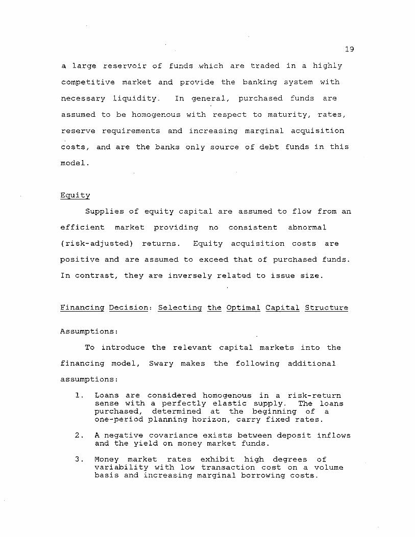
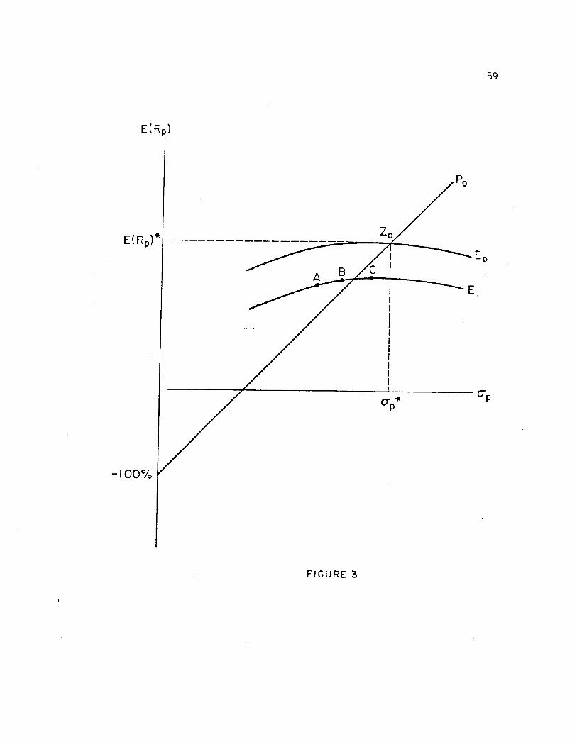
As shown by Roy (1952), Blair and Heggestad (1978) and Kahane (1977), P corresponds to the upper level of the probability of failure and is defined as the reciprocal of the slope of a ray in mean variance space. Graphically, Figure 3, this ray must intercept the return axis at -1 (signifying -100 percent return on assets).

10 0 %

FIGURE 3

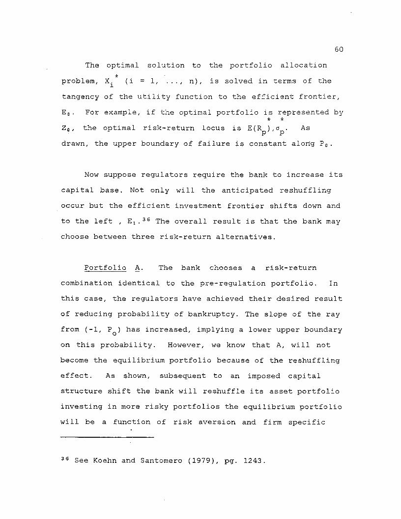
60The optimal solution to the portfolio allocation

•kproblem, (i = 1, . . . , n) , is solved in terms of thetangency of the utility function to the efficient frontier,E 0. For example, if the optimal portfolio is represented by

* *Z 0, the optimal risk-return locus is E(R ),a . Asp pdrawn, the upper boundary of failure is constant along P 0.

Now suppose regulators require the bank to increase its capital base. Not only will the anticipated reshuffling occur but the efficient investment frontier shifts down and to the left , E x.36 The overall result is that the bank may choose between three risk-return alternatives.

Portfolio A. The bank chooses a risk-return combination identical to the pre-regulation portfolio. In this case, the regulators have achieved their desired result of reducing probability of bankruptcy. The slope of the ray from (-1, PQ ) has increased, implying a lower upper boundary on this probability. However, we know that A, will not become the equilibrium portfolio because of the reshuffling effect. As shown, subsequent to an imposed capital structure shift the bank will reshuffle its asset portfolio investing in more risky portfolios the equilibrium portfolio will be a function of risk aversion and firm specific

36 See Koehn and Santomero (1979), pg. 1243.

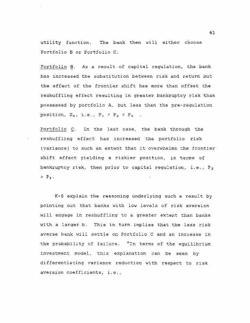
61utility function. The bank then will either choose Portfolio B or Portfolio C.

Portfolio B. As a result of capital regulation, the bank has increased the substitution between risk and return but the effect of the frontier shift has more than offset the reshuffling effect resulting in greater bankruptcy risk than possessed by portfolio A, but less than the pre-regulation position, Z 0, i.e., P : < P2 < Po

Portfolio C. In the last case, the bank through the reshuffling effect has increased the portfolio risk (variance) to such an extent that it overwhelms the frontier shift effect yielding a riskier position, in terms of bankruptcy risk, then prior to capital regulation, i.e., P 3> P„.

K-S explain the reasoning underlying such a result by pointing out that banks with low levels of risk aversion will engage in reshuffling to a greater extent than banks with a larger b. This in turn implies that the less risk averse bank will settle on Portfolio C and an increase in the probability of failure. "In terms of the equilibrium investment model, this explanation can be seen by differentiating variance reduction with respect to risk aversion coefficients, i.e.,

62d(dop 2/-dK)

_______________ >0 (58)

db

Thus, ap 2 declines for every bank's portfolio, but the absolute magnitude of the decline depends on b. However, if b is sufficiently small, the fall in E(Rp ) along with the reshuffling of the portfolio implies that the chance of failure increases."37 Based on these results, K-S propose two hypotheses:

1. Suppose that capital regulation was imposed uniformly across the industry. The preceding analysis suggest that reshuffling of asset portfolios would occur and the degree to which portfolio risk is increased is a function of the risk aversion parameter of the individual bank. In any case, the more risky banks will actually circumvent regulators intent and increase the riskiness of their asset portfolio to a greater extent thant their more risk-averse counterparts. The macro-industry implication of this hypothesis is that "the final distribution of risk of failure for the banking industry will therefore possess a higher dispersion than before the imposition of regulation."38

37 Koehn and Santomero (1979), pg. 1243.38 Koehn and Santomero (1979), pg. 1244.

632. Suppose instead that' regulators attempt to impose

capital regulation on that segment of the industry which possesses an excessive probability of bankruptcy. Also it may be safe to assume that this chosen sector exhibited low levels of risk aversion. Under the framework of analysis, such a hypothesis suggests that banks that are faced with non-market capital structure shifts because they are perceived to possess excessive levels of risk would react not by reducing their bankruptcy risk but by reshuffling their asset portfolio achieving even higher levels of bankruptcy risk. (Portfolio C).

It is this second hypothesis which provides the basis for the following empirical research. If a sample of banks can be isolated which experienced regulated capital structure increases, was there a corresponding reshuffling of their asset portfolio, as suggested by Swary, Edwards and Scott, Koehn and Santomero and O'Hara, relative to banks which experienced no such capital structure shift?

Chapter IVSAMPLE SELECTION AND EMPIRICAL TEST DESIGN

IntroductionChapters Two and Three analytically derived the

decision-making process of the commercial bank under two polar environments: a completely unregulated framework andunder a framework of various forms of balance sheet regulation. It was shown that in an unregulated world the commercial banks maximize their objective functions by equating the marginal return from the lending activity with the marginal cost of making a particular loan. And where marginal cost is defined as the reduction in market value attributable to the safety-first constraint, the bank explicitly incorporates the impact of risk 'in its lending policies. In contrast, the commercial bank operating in a regulated regime involving capital structure constraints, optimizes its objective function by equating marginal returns from loans with the marginal cost of acquiring debt and equity funds. Absent is the effect that the credit extension and its corresponding contribution to the riskiness of the asset (loan) portfolio has upon the default risk of the bank.

Of particular interest is the possible reaction a commercial bank may have to an exogenous change in its

64

65capital structure. While capital structure regulation actually constrains the permissible risky portfolios the bank may select, which could result in lowering the bank probability of default, the ability of the bank to somehow offset this effect becomes of primary importance. Specifically, that in response to an exogenous constraint on the mix of funds the bank is allowed to employ, the regulated bank will reshuffle its asset portfolio moving along the investment frontier as to actually increase its default risk. This chapter presents univariate and multivariate tests designed to determine the impact that capital structure regulation has upon the commercial banks asset portfolio decision, and in turn, attempts to measure whether the post-regulation portfolio exhibits greater default risk.

Formal Statement of the HypothesesIt has been suggested that a bank in response to a

exogenous shift in capital structure will reshuffle its asset portfolio as to invest in more risky assets. Further, this resulting asset portfolio may offset the intent of the regulation by increasing the regulated banks probability of default. Formally:

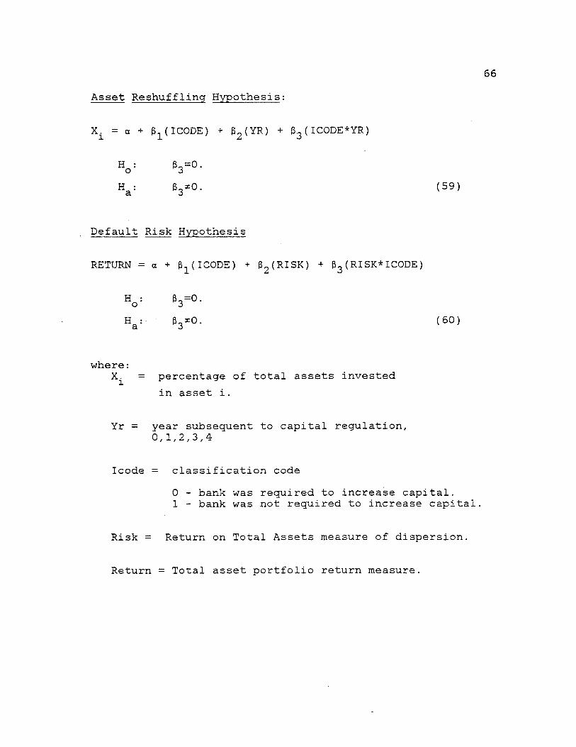
Asset Reshuffling Hypothesis:

X i = “ + &i(IC0DE) + 32 (YR) + &3 (icode*yr)

B3x °. (59)

Default Risk Hypothesis

RETURN = a + p (ICODE) + P2 (RISK) + &3 (RISK*ICODE)

Yr = year subsequent to capital regulation,0 ,1 ,2 ,3,4

Icode = classification code0 - bank was required to increase capital.1 - bank was not required to increase capita

Risk = Return on Total Assets measure of dispersion.

B3x°. (50)

where:= percentage of total assets invested

in asset i .

Return = Total asset portfolio return measure.

67Sample Selection

In order to test these hypotheses, a sample of banks which experienced a regulated capital structure change is required. As many researchers in the area of capital adequacy are frustratingly aware, such a sample of banks is not publicly available. Regulators feel that making such information public, identifying those banks which are forced or encouraged to increase capital would be contrary to their soundness objective. Therefore, a sample of banks which experienced a regulated change in capital structure was generated through a nationwide mail survey. Due to the fact there are over 14,000 commercial banks in the U.S., it was necessary to first screen the total universe of banks based on the following criteria.

Regulatory EnvironmentThere are four national regulatory agencies which have

varying degrees of control over the nation's commercial banks, the Federal Reserve, the FDIC, the Comptroller of Currency and the Securities and Exchange Commission. Each of these agencies have different and sometimes overlapping responsibilities with respect to the regulation of the banking industry. In an attempt to raise the level of homogeneity of the test sample, at least with respect to regulatory environment, it was decided to consider only

68nationally chartered banks for the final sample. While both the FDIC and Federal Reserve do have legal authority over some activities of nationally chartered banks, the Federal Reserve must also regulate state banks which are members of the Federal Reserve, while the FDIC is responsible for state and nationally chartered banks which may or may not be members of the Federal Reserve. Because of this intricate maze of governing bodies the banking community generally posits that the Federal Reserve and the FDIC relegate primary responsibility of nationally chartered banks to the Comptroller of Currency. In addition, by excluding all state chartered banks from the sample, the regulatory influence of fifty different state banking authorities need not be considered.

Data AvailabilityAn initial requirement of empirical tests involving

time series testing is a sufficiently continuous data base. Defining sufficient ex-ante is not always straight forward but visions of unlimited data must be tempered with the realities of accessible data. The largest bases of commercial bank data, both in terms of data elements and time period available, are the FDIC tapes which contain both annual Income Statements and Reports of Condition for all chartered banks from 1972-to the present. It was decided

69that the period 1972-81 would be sufficiently continuous, and therefore, as a second sample screen, only banks with continuous and complete data for 1972-1981 were eligible for inclusion in the final test sample.

Capital Structure ShiftGiven that the premise of the research at hand is

contingent upon first identifying a sample of banks which experienced a regulated capital structure shift, any screen based on this criteria may seem transparent. Therefore, in addition to the obvious time and financial constraints of a mail survey of this magnitude, a precise definition of capital structure shift both in terms of levels of significance and characteristics was deemed essential. And by casually observing the capital structures of banks throughout the country, it is not surprising that all banks are experiencing some degree of change in their capital structure.

The final criteria employed in selecting the sample to be surveyed were to have banks which experience in any one year between 1973-1980 an increase in its capital/total assets ratio of at least 25 percent,39 and to have sold common stock in the year of the 25 percent capital/total

39 It is hardly expected that larger banks, assets exceeding 1 billion dollars, would increase capital at this rate. Therefore, the scope of the study will be limited to small banks. (See tables 3 and 4).

70asset increase. It is important to note that capital is defined in the pure sense, i.e., capital equals retained earnings plus common stock accounts. Thus by requiring a stock issuance any observed shift in the capital ratio can only be as result of a pure equity increase.

Survey Results

Questionnaire ResultsBased on the three stage screen outlined in the

previous section, 511 nationally chartered banks were identified that experienced at least a 25 percent increase in capital/total assets and issued common stock. Each of these banks was sent a questionnaire which required the bank to (1) verify report of condition and income statement information from the FDIC data base (2) confirm that a common stock issue occurred in the year of the capital structure increase and (3) provide reason as to why the capital structure increase and subsequent equity issue took place. Although data verification was important, question three determined the actual test sample. The bank was given the choice of four reasons for the observed capital structure shift:

1. REGULATORY OFFICALS REQUIRED THAT MORE CAPITAL BE RAISED EXTERNALLY.

712. REGULATORY OFFICALS SUGGESTED THAT MORE

CAPITAL BE RAISED EXTERNALLY.

3. REGULATORY OFFICALS HAD NO DIRECT PART IN THE DECISION, BUT MANAGEMENT BELIEVED THAT THEY WOULD SOON SUGGEST OR REQUIRE ADDITION CAPITAL.

4. REGULATORY OFFICALS HAD NO DIRECT PART IN THE DECISION; IT WAS AN INTERNAL MANAGEMENT DECISION.

Out of a total of 511 questionnaires initially sent, 245 responses were received. Two weeks following the initial survey, a follow-up letter with an identical questionnaire was sent. As expected, the second mailing was far less successful and 55 additional responses were received. The breakdown by catagory of responses to question 3 is given in Table 1.

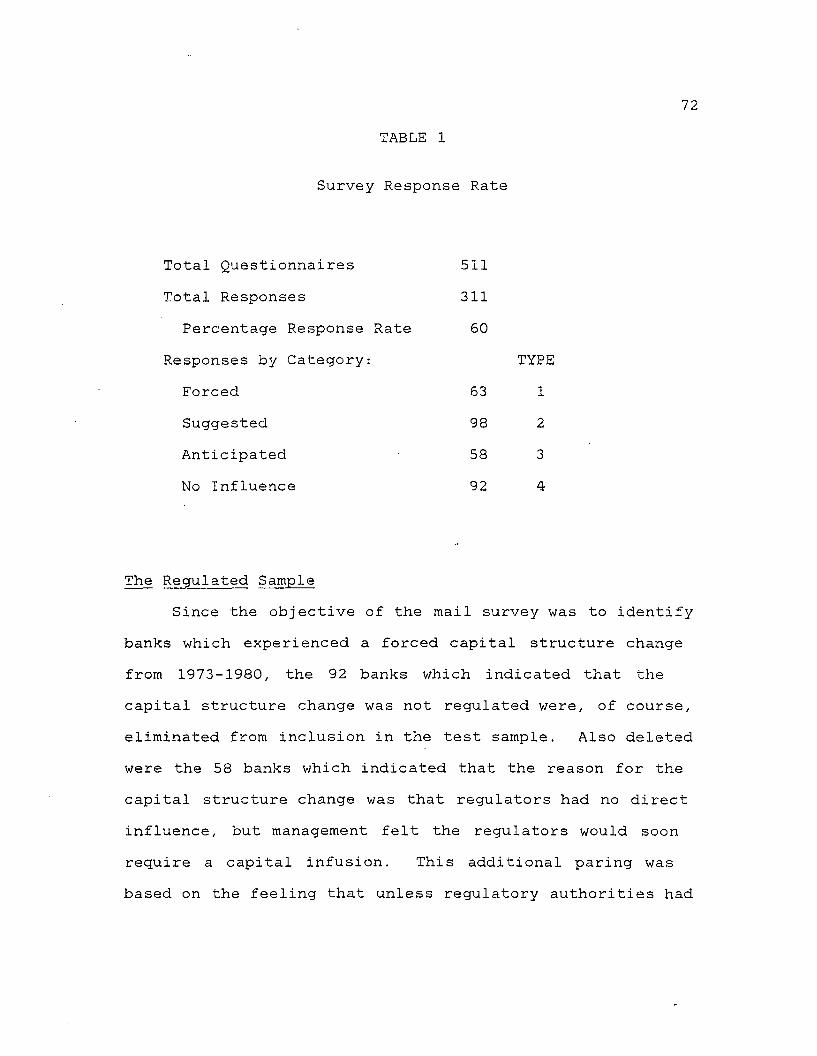
72TABLE 1

Survey Response Rate

Total Questionnaires 511Total Responses 311

Percentage Response Rate 60Responses by Category: TYPE

Eorced 63 1Suggested 98 2Anticipated 58 3No Influence 92 4

The Regulated SampleSince the objective of the mail survey was to identify

banks which experienced a forced capital structure change from 1973-1980, the 92 banks which indicated that the capital structure change was not regulated were, of course, eliminated from inclusion in the test sample. Also deleted were the 58 banks which indicated that the reason for the capital structure change was that regulators had no direct influence, but management felt the regulators would soon require a capital infusion. This additional paring was based on the feeling that unless regulatory authorities had

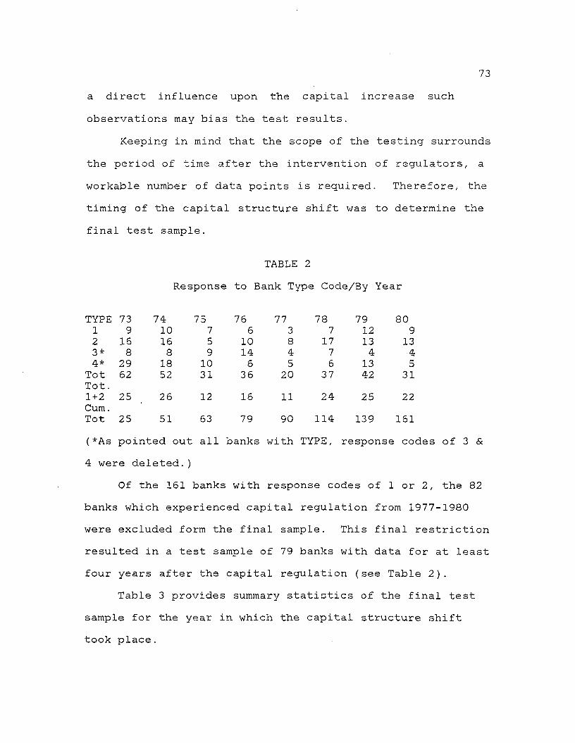
73a direct influence upon the capital increase such observations may bias the test results.

Keeping in mind that the scope of the testing surrounds the period of time after the intervention of regulators, a workable number of data points is required. Therefore, the timing of the capital structure shift was to determine the final test sample.

TABLE 2Response to Bank Type Code/By Year

TYPE 73 74 75 76 77 78 79 801 9 10 7 6 3 7 12 92 16 16 5 10 8 17 13 133* 8 8 9 14 4 7 4 .44 * 29 18 10 6 5 6 13 5

Tot 62 52 31 36 20 37 42 31Tot.1+2 25 26 12 16 11 24 25 22Cum. Tot 25 51 63 79 90 114 139 161( *As pointed out all banks with TYPE, response co<4 were deleted.)

Of the 161 banks with response codes of 1 or 2, the 82 banks which experienced capital regulation from 1977-1980 were excluded form the final sample. This final restriction resulted in a test sample of 79 banks with data for at least four years after the capital regulation (see Table 2).

Table 3 provides summary statistics of the final test sample for the year in which the capital structure shift took place.

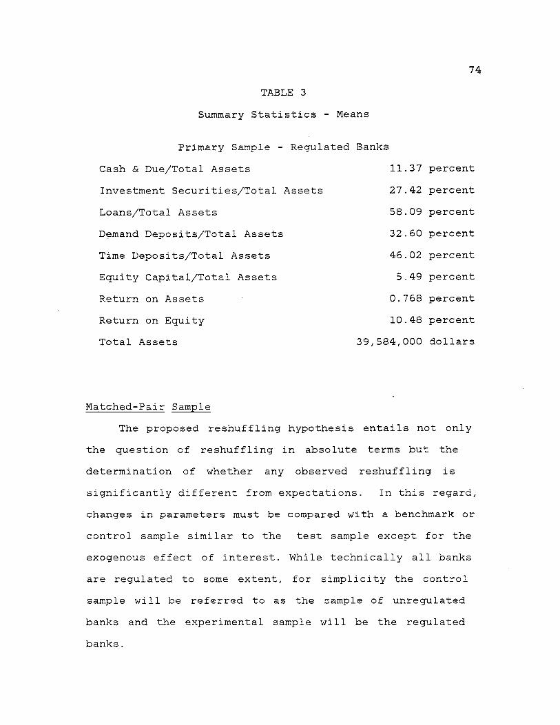
TABLE 3 Summary Statistics - Means

Primary Sample Cash & Due/Total Assets Investment Securities/Total Loans/Total Assets Demand Deposits/Total Assets Time Deposits/Total Assets Equity Capital/Total Assets Return on Assets Return on Equity Total Assets

- Regulated Banks11 .37 percent27 .42 percent58 .09 percent32 . 60 percent46 .02 percent5 . 49 percent

0 .768 percent10 . 48 percent

39,584, 000 dollars

Matched-Pair SampleThe proposed reshuffling hypothesis entails not only

the question of reshuffling in absolute terms but the determination of whether any observed reshuffling is significantly different from expectations. In this regard, changes in parameters must be compared with a benchmark or control sample similar to the test sample except for the exogenous effect of interest. While technically all banks are regulated to some extent, for simplicity the control sample will be referred to as the sample of unregulated banks and the experimental sample will be the regulated banks.

75With respect to capital- structure effects, the criteria

for identifying an unregulated bank was that (1) any increase in capital/total assets was less than 10 percent; and (2) the bank did not issue common stock from 1973-1980. To control for the regulatory environment, all banks in the control sample were required to be nationally chartered. To control economic and demographic factors, the matching bank had to be in the same state and, where appropriate, SMSA as the regulated bank. If the regulated bank was part of a holding company, then so must be the matching bank. The final criteria controlled for differences in size, measured by total assets.

Table 4 provides summary statistics for the unregulated sample for the year in which its matched pair experienced a regulated capital structure shift.

i

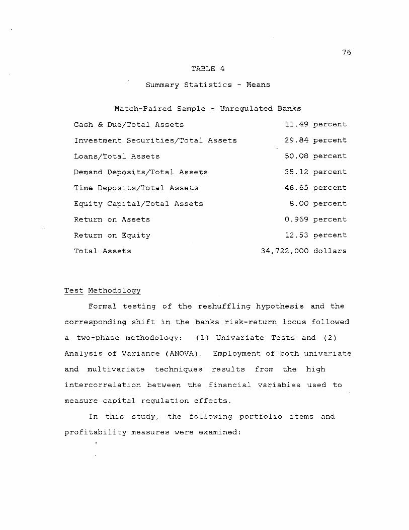
76TABLE 4

Summary Statistics - Means

Match-Paired Sample - Unregulated BanksCash & Due/Total Assets 11.49 percentInvestment Securities/Total Assets 29.84 percentLoans/Total Assets 50. 08 percentDemand Deposits/Total Assets 35. 12 percentTime Deposits/Total Assets 46. 65 percentEquity Capital/Total Assets 8.00 percentReturn on Assets 0. 969 percentReturn on Equity 12 .53 percentTotal Assets 34, 722,000 dollars

Test MethodologyFormal testing of the reshuffling hypothesis and the

corresponding shift in the banks risk-return locus followed a two-phase methodology: (1) Univariate Tests and (2)Analysis of Variance (ANOVA). Employment of both univariate and multivariate techniques results from the high intercorrelation between the financial variables used to measure capital regulation effects.

In this study, the following portfolio items and profitability measures were examined:

TABLE 5Assets Portfolio and Profitability Variables

Portfolio Composition1. Cash & Due from Banks/Total Assets2. Investment Securities/Total Assets3. U.S. Securities/Total Assets4. Goverment Agency Securities/Total Assets5. State & Political Subdivisions

Securities/Total Assets6 . Net Federal Funds/Total Assets7. Total Loans/Total Assets8 . Real Estate Loans/Total Assets9. Commercial Loans/Total Assets10. Consumer Loans/Total Assets11. Construction Loans/Total Assets12. Farm Loans/Total Assets13. Demand Deposits/Total Assets14. Savings Deposits/Total Assets15. Total Time Deposits/Total Assets16. Equity Capital/Total Assets17. Total Loans/Total Deposits18. Risky Assets/Total Assets

4

19. Total Assets20. Total Operating Revenue

B. Profitability Measures21. Return on Assets

7822. Return on Equity23. Operating Expenses/Operating Revenue24. Loan Losses/Total Loans25. Interest on Bonds, Notes & Securities/

Investment Securities26. Interest Paid on Borrowed Funds

Univariate TestsThe first tests of the reshuffling hypothesis are

intended to compare and contrast the portfolio holdings and profitability measures of the regulated and unregulated banks. This "first pass" at identifying the effects of regulation, while not possessing a great deal of explanatory power, should isolate significant differences between the bank samples which will be rigorously examined with multivariate testing procedures.

It is anticipated that (1) significant differences do exist in the year of regulation, t = 0 and, (2 ) if the observed capital regulation is effective, then more homogeneity exists between the financial variable in the post-regulatory years, t = 1,..,4. Hence, the tests should indicate differences at t = 0. Depending on the bank's response to the capital regulation, any changes in the bank's financial condition will be measured. It should be noted that the time required to adjust portfolio composition

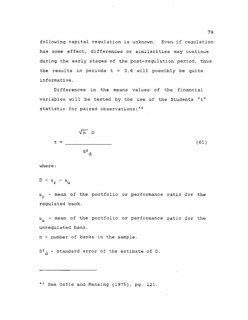
79following capital, regulation is unknown. Even if regulation has some effect, differences or similarities may continue during the early stages of the post-regulation period, thus the results in periods t = 3,4 will possibly be quite informative.

Differences in the means values of the financial variables will be tested by the use of the Students "t" statistic for paired observations:40

W Dt = ____ (61)

S2 b d

where:

D - v - y r u

y^ - mean of the portfolio or performance ratio for theregulated bank.

- mean of the portfolio or performance ratio for theunregulated bank.n - number of banks in the sample.

S2^ - standard error of the estimate of D.

40 See Ostle and Mensing (1975), pg. 121.

80Multivariate Tests

As widely known, one weakness of using the "t" test is the inability to make time series comparisons, i.e., given two periods and corresponding "t" statistics, the fact that one "t" is greater or less than the other does not imply a divergence or convergence between the time periods. In addition by analyzing a series of "t" statistics the relationships between variables is ignored and, as previously mentioned, the financial variables used in this research tend to be highly intercorrelated. Thus, multivariate tests will be employed to' account for the variations over time and between variables.

Analysis of VarianceThe univariate test discussed above only serves to

raise the suspicion that certain banks are reacting to capital structure regulation and this reaction takes the form of asset portfolio reshuffling. Analysis of variance techniques can also test not only for differences in mean values between groups but for changes in variables (means) between groups over time. With regard to the stated null hypotheses, the magnitude of these changes in portfolio composition shed light on the capital regulation issue.

Tha analysis of variance test will be conducted in two stages corresponding to the two null hypotheses: stage one

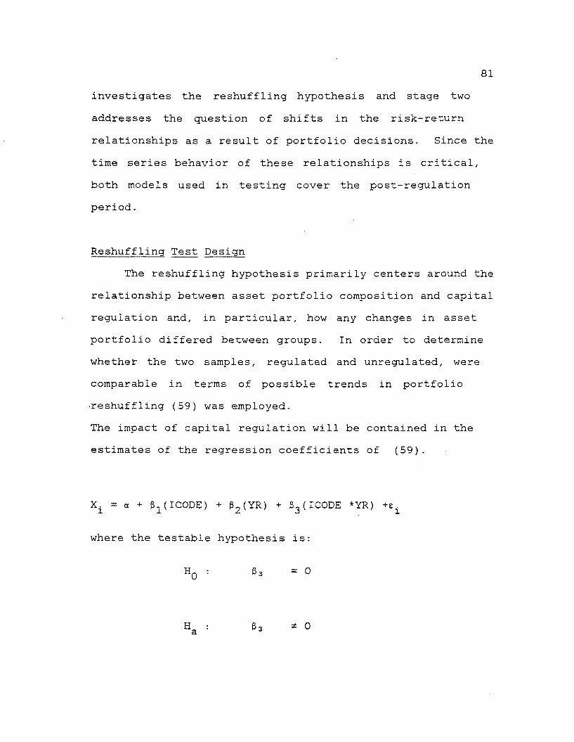
81investigates the reshuffling hypothesis and stage two addresses the question of shifts in the risk-return relationships as a result of portfolio decisions. Since the time series behavior of these relationships is critical, both models used in testing cover the post-regulation period.

Reshuffling Test DesignThe reshuffling hypothesis primarily centers around the

relationship between asset portfolio composition and capital regulation and, in particular, how any changes in asset portfolio differed between groups. In order to determine whether the two samples, regulated and unregulated, were comparable in terms of possible trends in portfolio •reshuffling (59) was employed.The impact of capital regulation will be contained in the estimates of the regression coefficients of (59).

Xi = a + 3X (ICODE) + S2 (YR) + 33 (ICODE *YR) +z±

where the testable hypothesis is:

Hq : e3 = 0

3 3 * 0

82The mean values of corresponding to different values

of the independent variables are:

E(X±|ICODE=0) = a + 02 (YR)

E(Xi|IC0DE=1) =(0+0!) + (02+03)(YR) andE(ei ) ^ N(0,a2)E(eiej ) = 0 , i*j

Interpretation of the regression coefficients are as follows:41a = mean value of X^ for the regulated sample

at t=0 .a+0! = mean value of X^ for the unregulated sample,

at t=0 .02 = estimate of the change in the mean of X^ (slope)

from the year of capital regulation to the end of the test period, t=0,..,t=4.

03 = estimate of the difference in the change in the meanof X^ for the unregulated sample vis-a-vis theregulated sample.

With respect to the reshuffling hypothesis, the estimate of interaction term, 03, is most informative. By construction, it is the interaction term which accounts for any differences in mean holdings of asset^ between the two samples subsequent to the imposition of capital regulation. Specifically, 03 significantly < 0 indicates an increase in

41 For a detailed proof of these equalities andinterpretations of the coefficients see Kmenta (1971), pg. 409-425.

83the holdings of asset^ by the regulated group vis-a-vis the unregulated sample during the post-regulation period. Conversly, if g3 is significantly > 0 then the unregulated groups' mean holdings of asset^ is increasing relative to the regulated group over the same test period.

Default-Risk ModelAs outlined in chapters two and three, Swary, Koehn and

Santomero, Scott and Edwards, and O'Hara suggest that banks react to regulatory imposed increases in capital, and as a result, reshuffles the asset portfolio thereby altering its risk-return locus. Even if asset portfolios reshuffling is detected, the issue remains whether the post-regulation portfolio has increased or decreased the underlying default risk of the regulated bank.

Before discussing the empirical model, the two parameters of the hypotheses must be defined, risk and return. In the financial or non-financial firm, return is generally defined as either return on assets, ROA, or return on equity, ROE. Given that the reshuffling hypothesis centers around fluctuations of holdings in the asset portfolio, ROA would seem appropriate as the overall measure of return. Further, inasmuch as default risk is defined where the return on assets is equal to -100 percent, tests involving the return series of the asset portfolio would

84provide information as to the direction of default probability.

The choice of the appropriate risk proxy is unfortunately not quite as straightforward. In defining risk there is a divergence resulting from the viewpoint taken. From the stockholders' position, the relevant measure of risk stems from portfolio theory.

Portfolio theory defines the relevant risk of an asset as beta, the covariance between the return on that individual asset and the returns on the market portfolio divided by the variance of the return on the market portfolio. In contrast, the regulatory agencies are primarily concerned not with stockholders1 risk but total risk, i.e., the risk that the bank will fail. Again, recalling that default probability is expressed in terms of ROA and variance of ROA, the relative dispersion of the ROA distribution will proxy for portfolio risk. Thus, multiple regression analysis will be used to determine whether any asset portfolio reshuffling exhibited by the regulated group resulted in a deterioration of the risk-return locus relative to unregulated banks. The regressors of ROA variable will be four measures of relative dispersion42 of

42 The use of estimates of the dispersion parameters yield regression estimates which are biased and lack the property of consistency. And traditional approaches to resolve these measurement error problems proved unsuccessful. See Neter and Wasserman (1974), p.168 for a discussion.

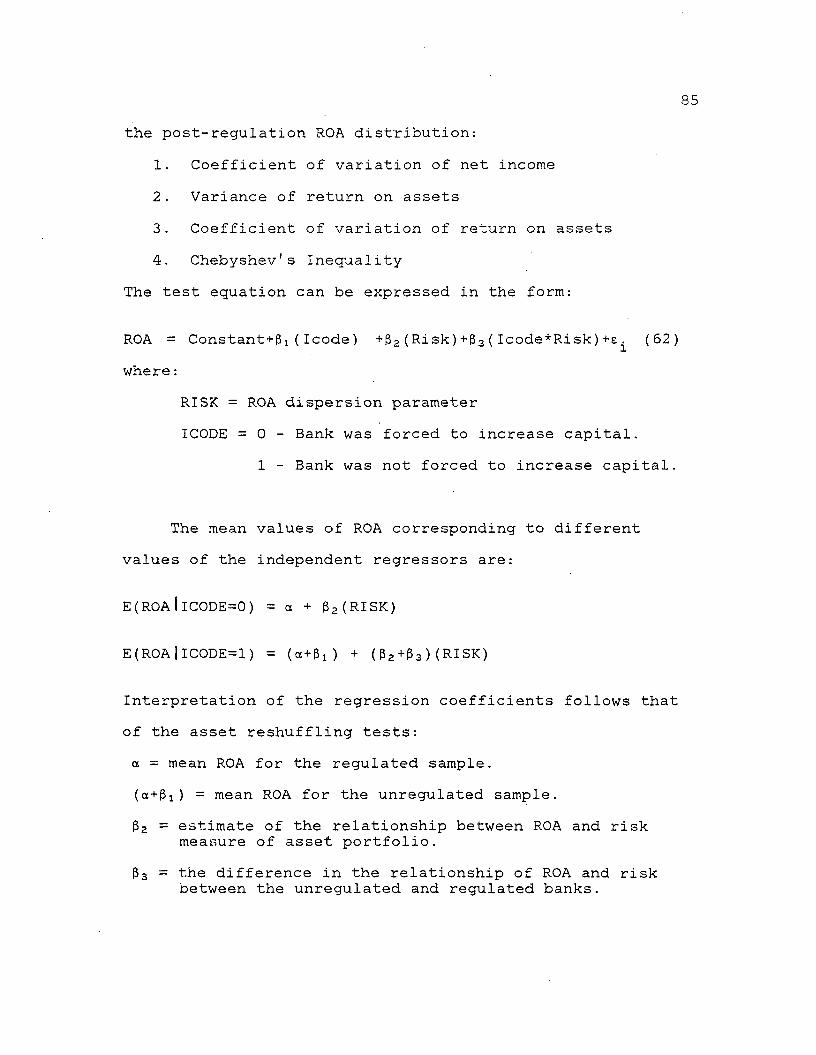
85the post-regulation ROA distribution:

1. Coefficient of variation of net income2. Variance of return on assets3. Coefficient of variation of return on assets4. Chebyshev's Inequality

The test equation can be expressed in the form:

ROA = Constant+3i(Icode) +g2(R i )+ &3(Icode*Risk)+s^ (62) where:

RISK = ROA dispersion parameterICODE = 0 - Bank was forced to increase capital.

1 - Bank was not forced to increase capital.

The mean values of ROA corresponding to different values of the independent regressors are:

E(ROAllCODE=0) = a + S2 (RISK)

E(ROA|IC0DE=1) = (a+Si) + (32+33)(RISK)

Interpretation of the regression coefficients follows thatof the asset reshuffling tests:a = mean ROA for the regulated sample.(a+3i) = mean ROA for the unregulated sample.(32 = estimate of the relationship between ROA and risk

measure of asset portfolio.$3 = the difference in the relationship of ROA and risk

between the unregulated and regulated banks.

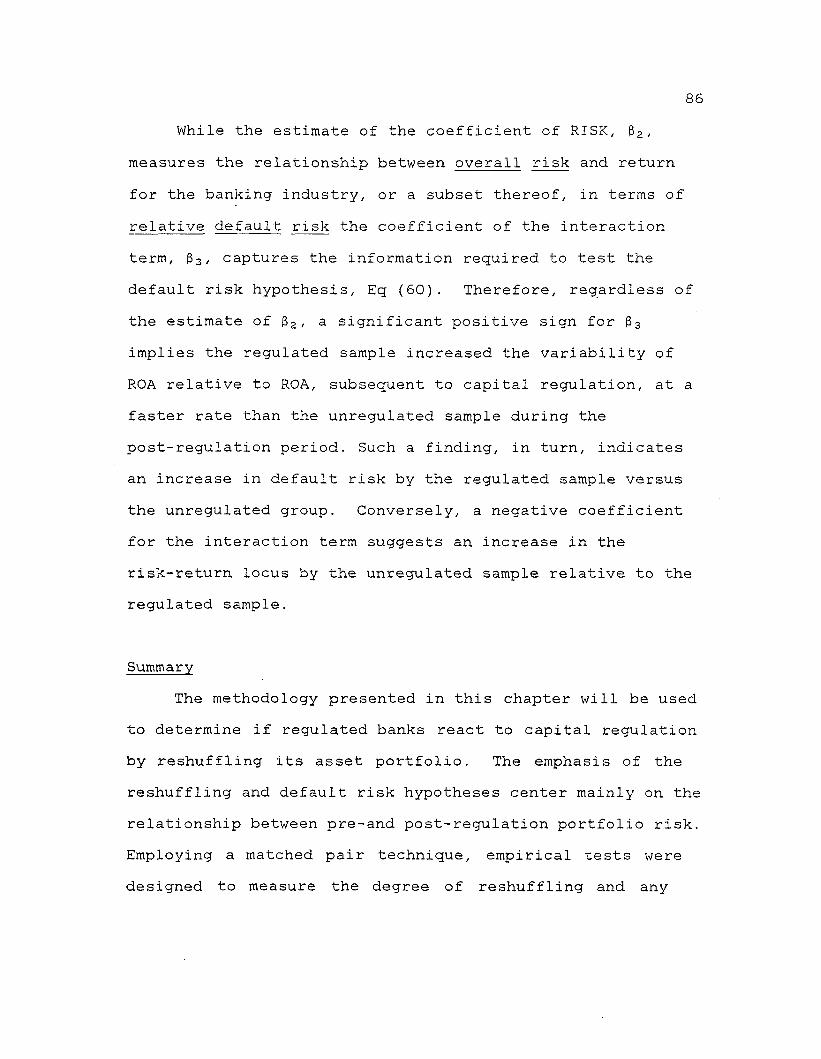
While the estimate of the coefficient of RISK, 32/ measures the relationship between overall risk and return for the banking industry, or a subset thereof, in terms of relative default risk the coefficient of the interaction term, 33/ captures the information required to test the default risk hypothesis, Eq (60). Therefore, regardless of the estimate of 32/ a significant positive sign for 33 implies the regulated sample increased the variability of ROA relative to ROA, subsequent to capital regulation, at a faster rate than the unregulated sample during the post-regulation period. Such a finding, in turn, indicates an increase in default risk by the regulated sample versus the unregulated group. Conversely, a negative coefficient for the interaction term suggests an increase in the risk-return locus by the unregulated sample relative to the regulated sample.

SummaryThe methodology presented in this chapter will be used

to determine if regulated banks react to capital regulation by reshuffling its asset portfolio. The emphasis of the reshuffling and default risk hypotheses center mainly on the relationship between pre-and post-regulation portfolio risk. Employing a matched pair technique, empirical tests were designed to measure the degree of reshuffling and any

87corresponding changes in default risk in response to capital regulation.

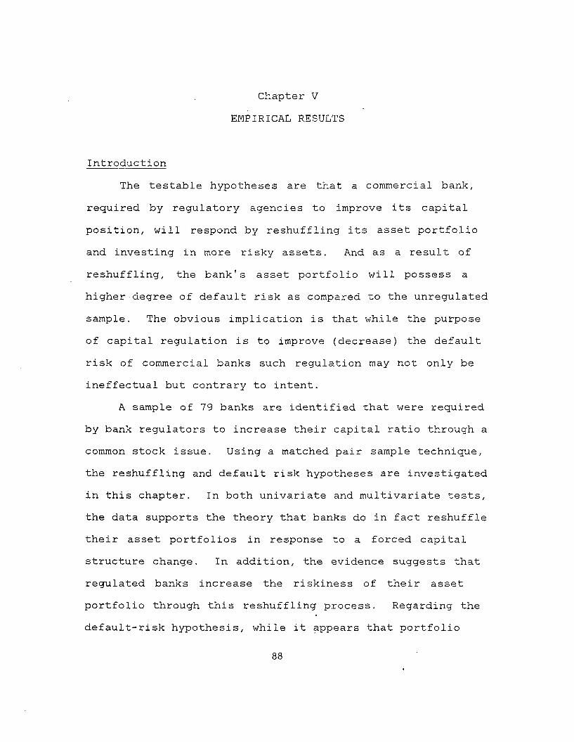
Chapter V EMPIRICAL RESULTS

IntroductionThe testable hypotheses are that a commercial bank,

required by regulatory agencies to improve its capital position, will respond by reshuffling its asset portfolio and investing in more risky assets. And as a result of reshuffling, the bank's asset portfolio will possess a higher degree of default risk as compared to the unregulated sample. The obvious implication is that while the purpose of capital regulation is to improve (decrease) the default risk of commercial banks such regulation may not only be ineffectual but contrary to intent.

A sample of 79 banks are identified that were required by bank regulators to increase their capital ratio through a common stock issue. Using a matched pair sample technique, the reshuffling and default risk hypotheses are investigated in this chapter. In both univariate and multivariate tests, the data supports the theory that banks do in fact reshuffle their asset portfolios in response to a forced capital structure change. In addition, the evidence suggests that regulated banks increase the riskiness of their asset portfolio through this reshuffling process. Regarding the default-risk hypothesis, while it appears that portfolio

88

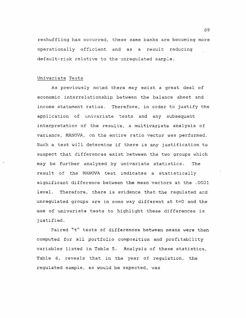
89reshuffling has occurred, these same banks are becoming more operationally efficient and as a result reducing default-risk relative to the unregulated sample.

Univariate TestsAs previously noted there may exist a great deal of

economic interrelationship between the balance sheet and income statement ratios. Therefore, in order to justify the application of univariate tests and any subsequent interpretation of the results, a multivariate analysis of variance, MANOVA, on the entire ratio vector was performed. Such a test will determine if there is any justification to suspect that differences exist between the two groups which may be further analyzed by univariate statistics. The result of the MANOVA test indicates a statistically significant difference between the mean vectors at the .0001

level. Therefore, there is evidence that the regulated and unregulated groups are in some way different at t=0 and the use of univariate tests to highlight these differences is justified.

Paired "t" tests of differences between means were then computed for all portfolio composition and profitability variables listed in Table 5. Analysis of these statistics, Table 6 , reveals that in the year of regulation, the regulated sample, as would be expected, was

strikingly different than the unregulated sample with respect to both asset composition and profitability. At the time of regulation, t = 0 , the regulated bank can be described as a bank which held fewer investment securities, therefore held a larger percentage of assets as loans, employed fewer demand deposits and more borrowed funds, were net sellers of federal funds and overall had a higher loan/deposit ratio. In terms of profitability, the regulated bank realized a lower return on investment securities, total assets and equity, experienced higher costs on borrowed funds and were less operationally efficient as reflected by a higher percentage of operating expenses to income. It is therefore reasonable to conclude that at t = 0 , regulated banks were overall riskier as indicated by the loan/deposit ratio and significantly less profitable as per return on assets and equity. This conclusion is hardly unexpected and, in fact, if contrary relationships were present, one would certainly question the reliability of the test sample. Although the precise factors behind a regulators intervention are not public information, it would be safe to assume that balance sheet and income statement data will highlight differences that would be a basis for regulatory action.

Recalling that the timing of the portfolio reshuffling process is unknown, differences or similarities in the

91subsequent years should not be viewed as necessarily supportive or contrary with the stated hypotheses. Instead, it has been suggested that an adjustment period of one or two years be introduced to allow the firms reaction, if any exists, to regulation to take effect on its financial structure. Therefore, it is anticipated that while the effects of some decisions will appear rapidly, the overall reaction of the regulated bank sample may not be observed until some three or four years subsequent to the forced capital structure change, t = 3,4. Thus, in order to determine whether the "t" tests reflect on either the reshuffling or default risk hypothesis, data from the entire post-regulation period must be examined.

There are significant changes occurring in periods t = 1 and t = 2 which reflect on the reshuffling hypothesis. One year after regulation, the regulated sample, while retaining the vast majority of differences in portfolio composition from the base year, did increase its dependence upon demand deposits as a financing source and has altered its profitability characteristics. In particular, it is observed from Table 6 that regulated banks have increased gross yield on earning assets primarily due to a higher rate of return on its securities investment portfolio. As will be argued and tested in a later section, this result suggests some degree of reshuffling of the investment

92portfolio toward riskier securities. The contention is that in order to realize higher returns the portfolio must possess more risk.

)

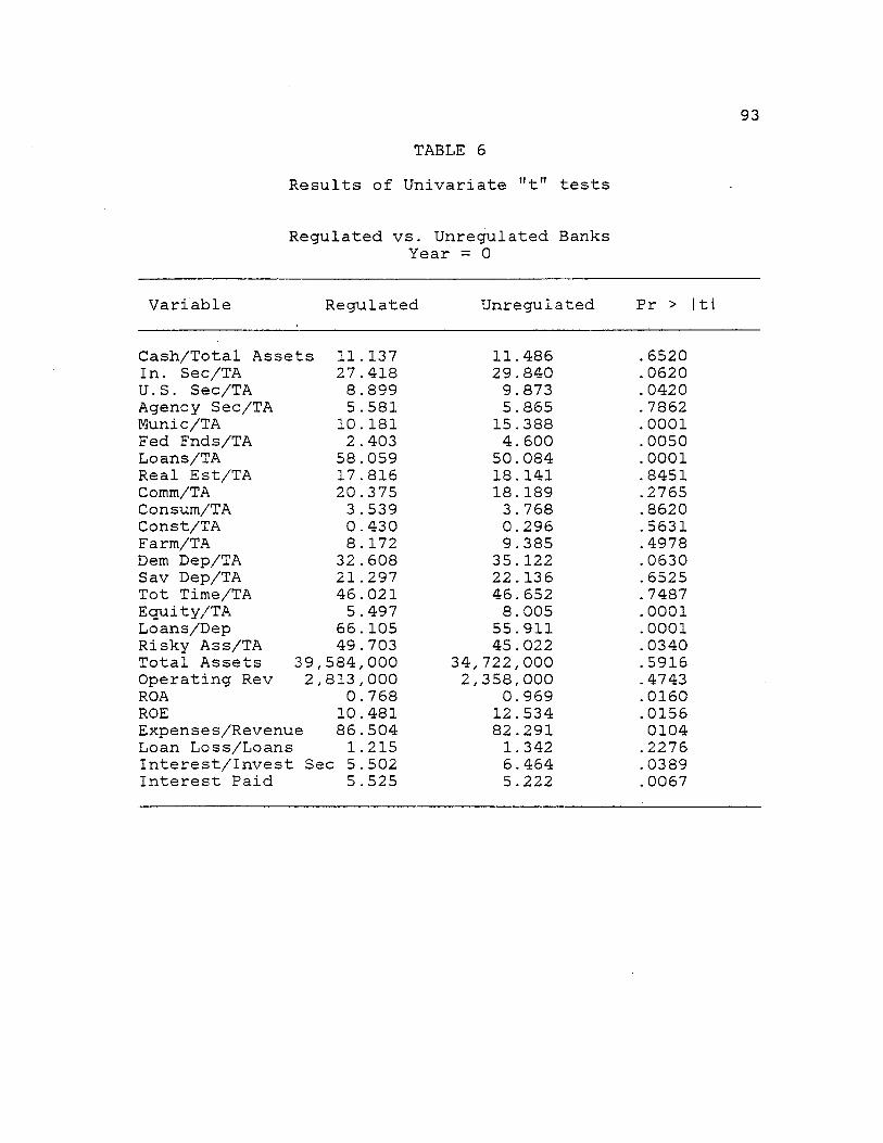
93TABLE 6

Results of Univariate "t" tests

Regulated vs. Unregulated Banks Year = 0

Variable Regulated Unregulated Pr > |tl

Cash/Total Assets 11.137 11.486 .6520In. Sec/TA 27.418 29.840 .0620U.S. Sec/TA 8.899 9.873 .0420Agency Sec/TA 5 .581 5.865 . 7862Munic/TA 10.181 15.388 . 0001Fed Fnds/TA 2 . 403 4. 600 . 0050Loans/TA 58.059 50.084 . 0001Real Est/TA 17.816 18.141 .8451Comm/TA 20.375 18.189 .2765Consum/TA 3 .539 3 . 768 .8620Const/TA 0.430 0.296 .5631Farm/TA 8 . 172 9.385 .4978Dem Dep/TA 32.608 35.122 .0630Sav Dep/TA 21.297 22.136 . 6525Tot Time/TA 46.021 46.652 . 7487Equity/TA 5 .497 8 . 005 .0001Loans/Dep 66.105 55.911 .0001Risky Ass/TA 49.703 45.022 .0340Total Assets 39,584,000 34,722,000 .5916Operating Rev 2, 813,000 2,358,000 .4743ROA 0 . 768 0.969 .0160ROE 10.481 12.534 .0156Expenses/Revenue 86.504 82.291 0104Loan Loss/Loans 1 .215 1. 342 .2276Interest/Invest Sec 5.502 6.464 .0389Interest Paid 5 . 525 5.222 .0067

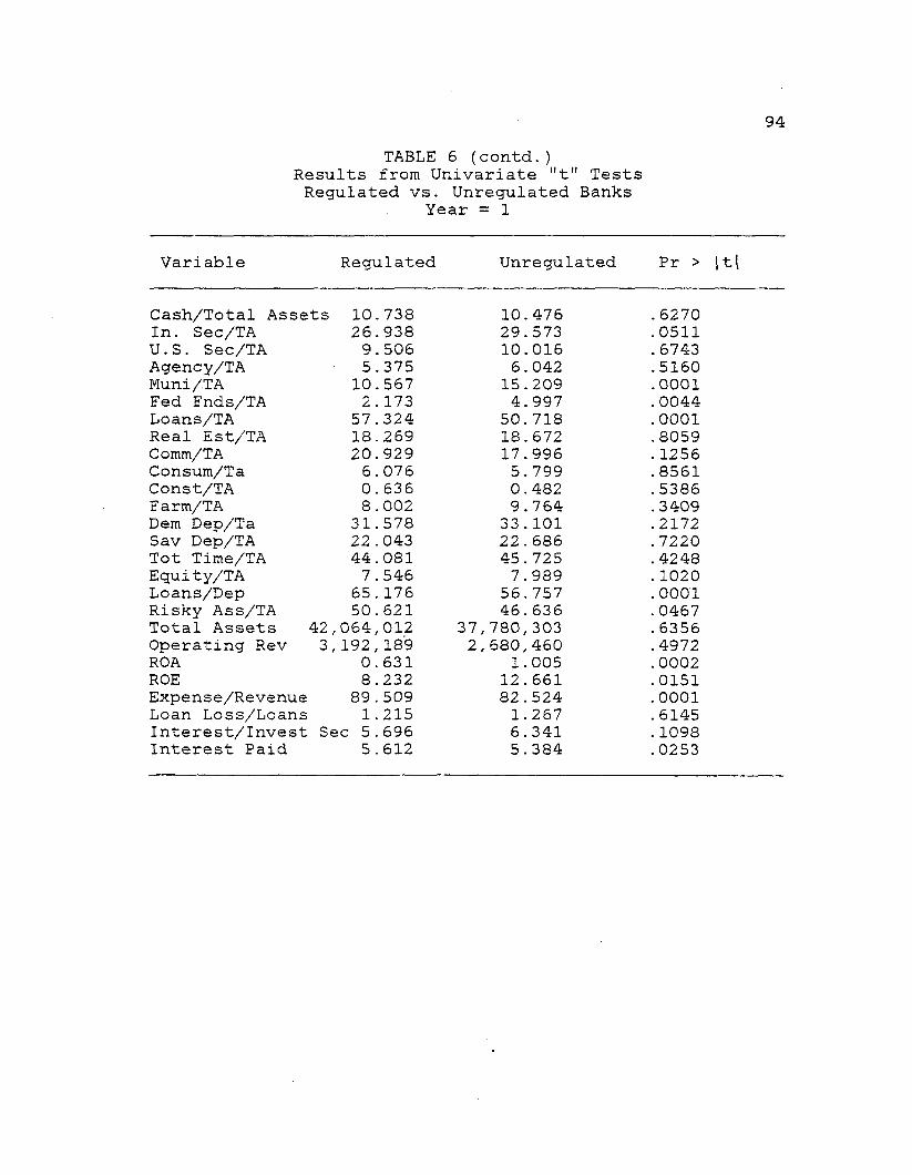
94TABLE 6 (contd.)

Results from Univariate "t" Tests Regulated vs. Unregulated Banks

Year = 1

Variable Regulated Unregulated Pr > |t(

Cash/Total Assets 10.738 10.476 .6270In. Sec/TA 26.938 29.573 .0511U.S. Sec/TA 9.506 10.016 . 6743Agency/TA 5.375 6.042 .5160Muni /.T A 10.567 15.209 .0001Fed Fnds/TA 2. 173 4. 997 . 0044Loans/TA 57.324 50.718 .0001Real Est/TA 18.269 18.672 . 8059Comm/TA 20.929 17.996 . 1256Consum/Ta 6.076 5. 799 .8561Const/TA 0. 636 0.482 . 5386Farm/TA 8.002 9 . 764 . 3409Dem Dep/Ta 31.578 33.101 .2172Sav Dep/TA 22.043 22.686 . 7220Tot Time/TA 44.081 45.725 .4248Equity/TA 7.546 7 . 989 . 1020Loans/Dep 65.176 56.757 . 0001Risky Ass/TA 50.621 46.636 .0467Total Assets 42,064,012 37,780,303 . 6356Operating Rev 3,192,189 2,680,460 .4972ROA 0. 631 1.005 .0002ROE 8.232 12.661 . 0151Expense/Revenue 89.509 82.524 .0001Loan Loss/Loans 1.215 1. 267 . 6145Interest/Invest Sec 5.696 6.341 . 1098Interest Paid 5 . 612 5.384 .0253

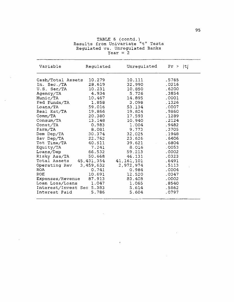
95TABLE 6 (contd.)

Results from Univariate "t" Tests Regulated vs. Unregulated Banks

Year = 2

Variable Regulated Unregulated Pr > |t[

Cash/Total Assets 10.279 10.Ill .5765In. Sec./TA 28.619 32.990 .0216U.S. Sec/TA 10.231 10.850 . 6200Agency/TA 4. 934 5. 726 .3854Munic/TA 10.467 14.895 . 0001Fed Funds/TA 1. 858 3 . 098 . 1326Loans/TA 59.016 53.134 .0007Real Est/TA 19.866 19.824 . 9860Comm/TA 20.380 17.593 . 1289Consum/TA 13.148 10.940 .2124Const/TA 0.983 1.004 .9482Farm/TA 8.081 9 . 773 .3705Dem Dep/TA 30.374 32.025 . 1948Sav Dep/TA 22.762 23.626 . 6406Tot Time/TA 40.511 39.621 . 6804Eguity/TA 7 .241 8 . 016 . 0053Loans/De'p 66.532 59.213 . 0002Risky Ass/TA 50.668 46.131 . 0323Total Assets 45,431,354 41,161,101 . 6491Operating Rev 3, 459,632 2,972,974 .5113ROA 0.741 0. 984 .0004ROE 10.691 12.520 .0347Expenses/Revenue 87.913 83.408 . 0002Loan Loss/Loans 1.047 1.065 .8540Interest/Invest Sec 5.383 5. 614 .5862Interest Paid 5.786 5 . 604 . 0797

I

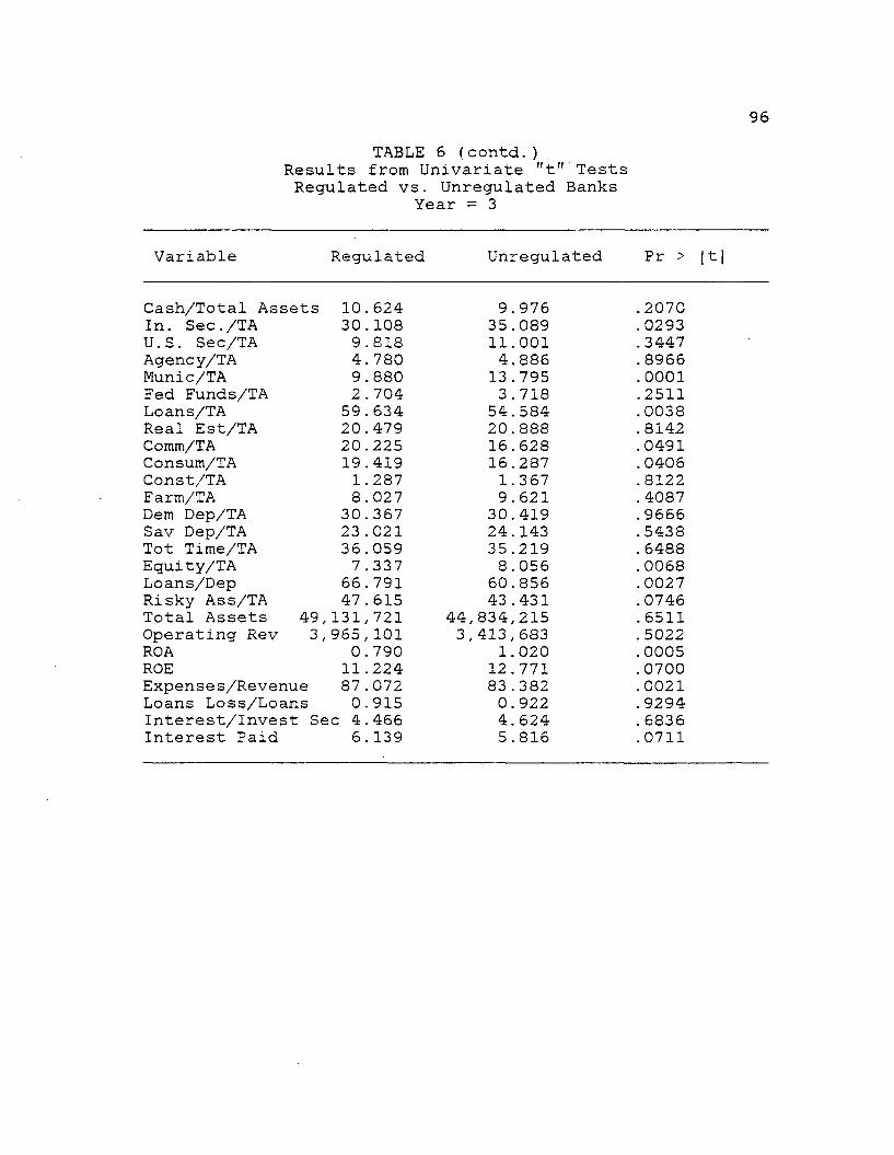
96TABLE 6 (contd.)

Results from Univariate "t" Tests Regulated vs. Unregulated Banks

Year = 3

Variable Regulated Unregulated Pr > |t|

Cash/Total Assets 10.624 9.976 .2070In. Sec./TA 30.108 35.089 .0293U.S. Sec/TA 9.818 11.001 .3447Agency/TA 4. 780 4.886 . 8966Munic/TA 9.880 13.795 . 0001Fed Funds/TA 2 . 704 3 . 718 .2511Loans/TA 59.634 54.584 .0038Real Est/TA 20.479 20.888 .8142Comm/TA 20.225 16.628 .0491Consum/TA 19.419 16.287 .0406Const/TA 1.287 1.367 .8122Farm/TA 8 . 027 9. 621 . 4087Dem Dep/TA 30.367 30.419 . 9666Sav Dep/TA 23.021 24.143 .5438Tot Time/TA 36.059 35.219 . 6488Equity/TA 7 . 337 8.056 . 0068Loans/Dep 66.791 60.856 .0027Risky Ass/TA 47.615 43.431 .0746Total Assets 49,131,721 44,834,215 .6511Operating Rev 3, 965,101 3,413,683 .5022ROA 0. 790 1.020 .0005ROE 11 .224 12.771 .0700Expenses/Revenue 87.072 83.382 .0021Loans Loss/Loans 0.915 0.922 . 9294Interest/Invest Sec 4.466 4. 624 . 6836Interest Paid 6 . 139 5.816 . 0711

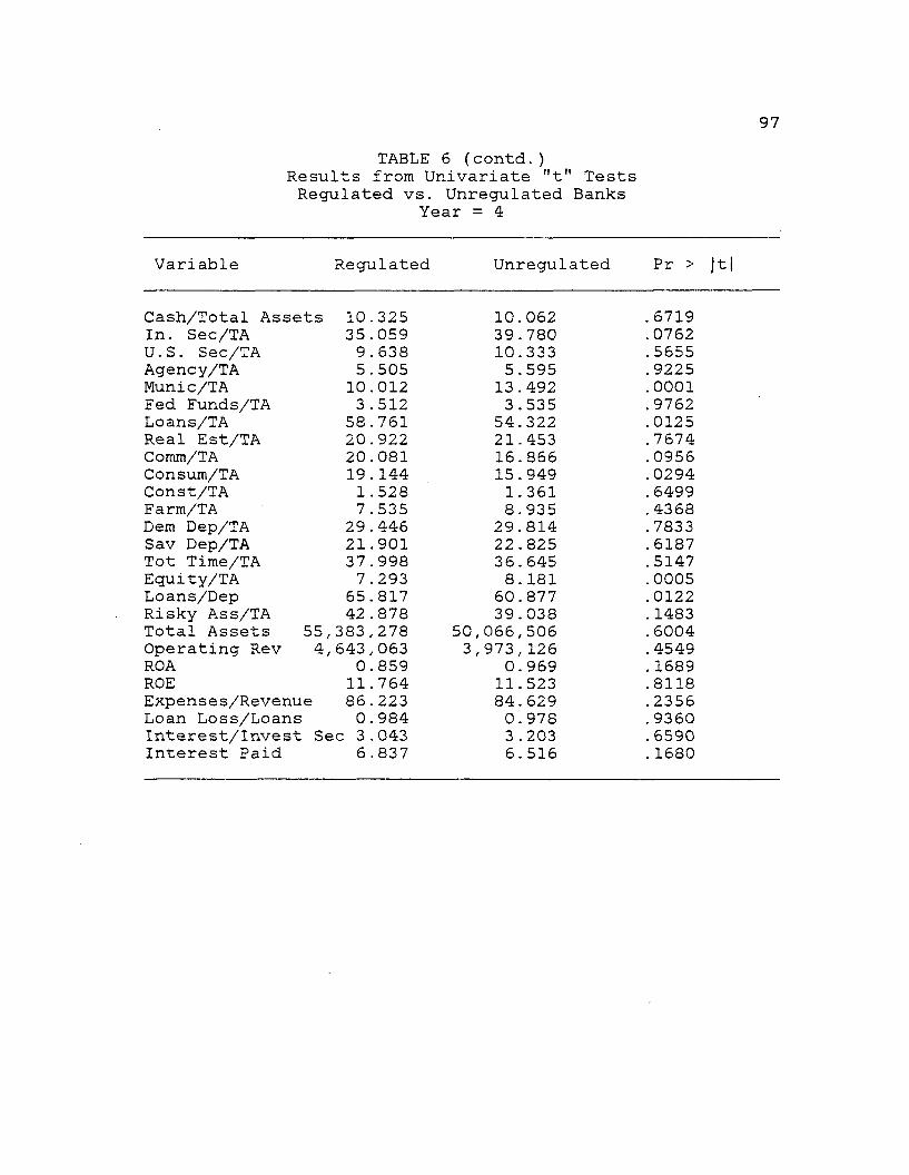
97TABLE 6 (contd.)

Results from Univariate "t" Tests Regulated vs. Unregulated Banks

Year = 4

Variable Regulated Unregulated Pr > Jt|

Cash/Total Assets 10.325 10.062 . 6719In. Sec/TA 35.059 39.780 .0762U.S. Sec/TA 9.638 10.333 .5655Agency/TA 5 .505 5.595 .9225Munic/TA 10.012 13.492 .0001Fed Funds/TA 3 .512 3.535 .9762Loans/TA 58.761 54.322 .0125Real Est/TA 20.922 21.453 .7674Comm/TA 20.081 16.866 .0956Consum/TA 19.144 15.949 .0294Const/TA 1 .528 1.361 . 6499Farm/TA 7 .535 8.935 .43 68Dem Dep/TA 29.446 29.814 . 7833Sav Dep/TA 21.901 22.825 .6187Tot Time/TA 37.998 36.645 .5147Equity/TA 7 .293 8 . 181 .0005Loans/Dep 65.817 60.877 . 0122Risky Ass/TA 42.878 39.038 . 1483Total Assets 55,383,278 50,066,506 . 6004Operating Rev 4, 643,063 3,973,126 .4549ROA 0.859 0. 969 . 1689ROE 11.764 11.523 .8118Expenses/Revenue 86.223 84.629 .2356Loan Loss/Loans 0.984 0. 978 .9360Interest/Invest Sec 3.043 3 .203 .6590Interest Paid 6.837 6 . 516 . 1680

98Moving to the second po'st-regulation year, not only

were the observed changes in profitability during year one retained a certain amount of portfolio reshuffling has taken place The beginnings of a reversal in the federal funds investment policy appears as the mean for the regulated bank falls from 2.173 percent to 1.857 percent. Foreshadowing the results from t = 3,4, this shift in federal funds holdings continues until the mean holdings are approximately identical. Two other changes in investment policy occur between the first and second year. The regulated banks have increased investment in real estate loans and municipal securities.As these changes relate to portfolio risk it would be safe to categorize real estate loans as a relatively high risk investment. In aggregate, the change in municipals would appear to imply lower risk. However, it is possible that the municipal securities selected by the regulated banks actually possess more risk relative to the unregulated banks' municipal portfolio. This municipal reshuffling argument is consistent with the results from t = 0 to t = 1 that revealed regulated banks increasing the yield from investment securities portfolio and will be tested further with the regression models.

Additional indications of increased asset portfolio risk through reshuffling are observed during years 3 and 4 as the regulated banks increase their commercial and consumer loans. Coupled with the fact that regulated

99banks .also experienced increases in the return on assets and equity suggest evidence as to the direction of asset portfolio risk. This evidence is however not conclusive inasmuch as the regulated banks also became more efficient, reducing operating expenses, during this time period which may account for the rise in profitability.

Overall, the results of the univariate tests provide a solid foundation to suspect that a significant amount of reshuffling is occurring by the regulated sample.Table 7 presents a summary of the findings of the univariate tests. Highlighted are the ratios which exhibited significant behavior in year 0 and years 1-4.

Proportional investments in assets catagories traditionally viewed as risky; real estate, commercial and consumer loans were on the rise by the regulated sample. Further, it is suggested that such an investment strategy viewed in light of increasing returns on assets and equity denotes that loan portfolios of regulated banks were becoming more risky. Also the investment securities portfolio provided some support for rejecting the null hypothesis of insignificant reshuffling by the regulated sample. It was observed that, while no implications can be drawn solely from the fact that regulated banks were increasing investment in municipal securities, the rise in the yield on the investment portfolio may indicate increased risk.

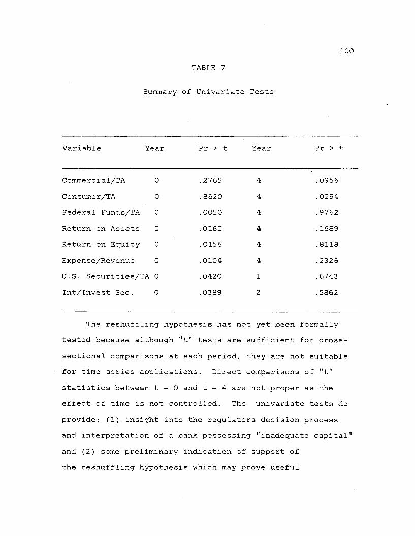
100TABLE 7

Summary of Univariate Tests

Variable Year Pr > t Year Pr > t

Commercial/TA 0 .2765 4 . 0956Consumer/TA 0 .8620 4 .0294Federal Funds/TA 0 .0050 4 .9762Return on Assets 0 .0160 4 . 1689Return on Equity 0 .0156 4 .8118Expense/Revenue 0 .0104 4 .2326U.S. Securities/TA 0 .0420 1 . 6743Int/Invest Sec. 0 .0389 2 .5862

The reshuffling hypothesis has not yet been formally tested because although "t" tests are sufficient for cross- sectional comparisons at each period, they are not suitable for time series applications. Direct comparisons of "t" statistics between t = 0 and t = 4 are not proper as the effect of time is not controlled. The univariate tests do provide: (1) insight into the regulators decision processand interpretation of a bank possessing "inadequate capital" and (2) some preliminary indication of support of the reshuffling hypothesis which may prove useful

101in interpretation and subsequent empirical testing.

Multivariate TestTest of Reshuffling Hypothesis

As pointed out, the preceding univariate testing of Eq. (61) does not permit any time-series comparisons of portfolio composition or profitability measures because of the inability of these to account for differences in the timing of observations. The use of multiple regression models to estimate relationships between variables overcomes this apparent weakness of the univariate tests. Properly specified, the coefficients from a multiple regession model measure the relationship between the dependent variable and the independent variable while holding the effects of the other independent variables constant.43 Thus (59) was chosen as an appropriate model for direct testing of the reshuffling hypothesis as it measures differences in assets holdings both across samples and between time periods. Further, and most fundamental to the testing of the reshuffling hypothesis is not whether regulated banks are changing the composition of their asset portfolio subsequent to capital regulation but how these changes differ from a sample of similar unregulated banks over the same time-

4 3 See the MANOVA test in the previous section for ajustification as to overall differences between meanvectors.

102period.

X i = constant + ^(Icode) +$2(Yr) + $3(Icode*Yr) +s^

where:- percentage of total assets invested

in asset i.Yr - year subsequent to capital regulation, 0,1,2,3,4.

Icode- classification code0 - bank required to increase capital1 - bank was not required to increase capital

Initially, the portfolio composition and profitability variables from Table 5 were introduced into Eq. (59) as dependent variables and were regressed on sample affiliation (regulated or unregulated), year (t = 0,1,2,3,4), and an interaction term, (sample affiliation multiplied by year). As discussed previously, it is the interaction term which accounts for any differences in changes of portfolio holdings between groups over time. A positive value of the interaction coefficient, (53, would indicate that the unregulated sample increased its investment in asset i relative to the regulated sample during the post-regulation period. Conversely, g3 < 0 indicates that the regulated samples' holdings of asset i grew faster than the unregulated sample. Results of the regressions of Eq. (59) are presented in Table 8.

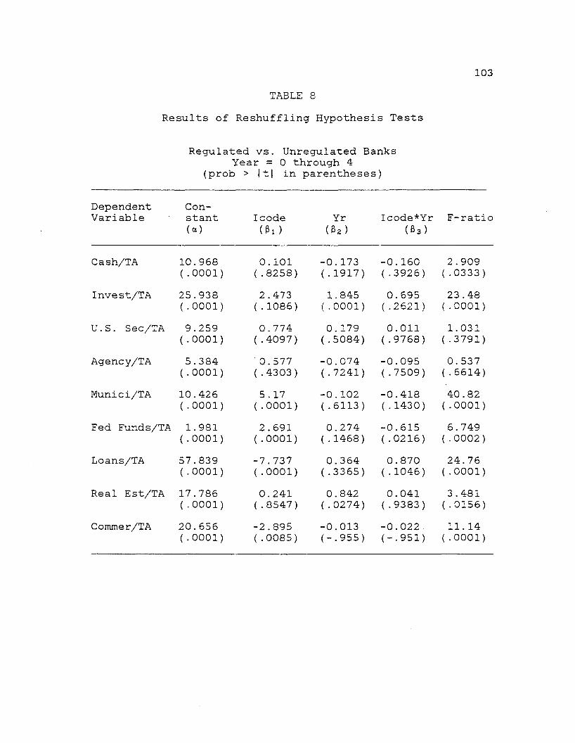
103TABLE 8

Results of Reshuffling Hypothesis Tests

Regulated vs. Unregulated Banks Year = 0 through 4

(prob > It| in parentheses)

DependentVariable

Con­stant(a)

Icode(Pi )

Yr(P2)

Icode*Yr(03)

F-ratio

Cash/TA 10.968 (.0001)

0. 101 (.8258)

-0.173 (.1917)

-0.160 ( . 3926)

2 .909 (.0333)

Invest/TA 25.938 (.0001)

2 . 473 (.1086)

1.845 (.0001)

0.695 ( .2621)

23 . 48 (.0001)

U.S. Sec/TA 9.259 (.0001)

0. 774 (.4097)

0. 179 (.5084)

0. 011 (.9768)

1. 031 ( .3791)

Agency/TA 5.384 (.0001)

'0.577 (.4303)

-0.074 (.7241)

-0.095 (.7509)

0.537 (.6614)

Munici/TA 10.426 (.0001)

5. 17 (.0001)

-0.102 (.6113)

-0.418 (.1430)

40 .82 (.0001)

Fed Funds/TA 1.981 (.0001)

2 . 691 (.0001)

0.274 (.1468)

-0.615 (.0216)

6. 749 (.0002)

Loans/TA 57.839 (.0001)

-7.737 (.0001)

0. 364 ( .3365)

0. 870 (.1046)

24. 76 (.0001)

Real Est/TA 17.786 (.0001)

0.241 (.8547)

0. 842 (.0274)

0.041 ( . 9383)

3.481 (.0156)

Commer/TA 20.656 (.0001)

-2.895 (.0085)

-0.013(-.955)

-0.022(-.951)

11. 14 (.0001)

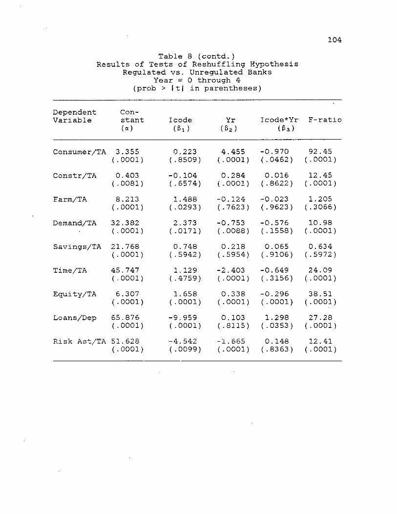
104Table 8 (contd.)

Results of Tests of Reshuffling Hypothesis Regulated vs. Unregulated Banks

Year = 0 through 4 (prob > lt| in parentheses)

DependentVariable

Con­stant(a)

Icode(3i)

Yr(32 )

Icode*Yr(P3)

F-ratio

Consumer/TA 3 .355 0.223 4.455 -0.970 92 .45(.0001) (.8509) (.0001) (.0462) (.0001)

Constr/TA 0.403 -0.104 0.284 0.016 12.45(.0081) (.6574) (.0001) (.8622) (.0001)

Farm/TA 8.213 1.488 -0.124 -0.023 1.205(.0001) (.0293) (.7623) (.9623) (.3066)

Demand/TA 32.382 2.373 -0.753 -0.576 10. 98( .0001) (.0171) (.0088) (.1558) (.0001)

Savings/TA 21.768 0. 748 0.218 0.065 0. 634(.0001) (.5942) (.5954) (.9106) ( .5972)

Time/TA 45.747 1. 129 -2.403 -0.649 24.09(.0001) (.4759) (.0001) (.3156) (.0001)

Equity/TA 6.307 1. 658 0.338 -0.296 38. 51(.0001) (.0001) (.0001) (.0001) (.0001)

Loans/Dep 65.876 -9.959 0. 103 1.298 27.28(.0001) (.0001) (.8115) (.0353) (.0001)

Risk Ast/TA 51.628 -4.542 -1.665 0. 148 12 . 41(.0001) (.0099) (.0001) (.8363) (.0001)

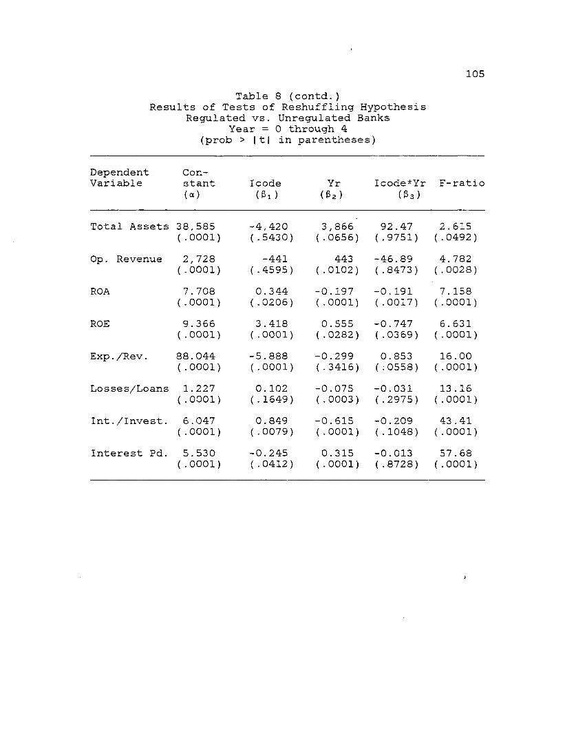
105Table 8 (contd.)

Results of Tests of Reshuffling Hypothesis Regulated vs. Unregulated Banks

Year = 0 through 4 (prob > It| in parentheses)

DependentVariable

Con­stant(a)

Icode (3i )

Yr(Pz)

Icode*Yr(33)

F-ratio

Total Assets 38,585 (.0001)

-4,420 (.5430)

3 , 866 (.0656)

92 .47 (.9751)

2 . 615 ( .0492)

Op . Revenue 2, 728 (.0001)

-441 (.4595)

443 (.0102)

-46.89 (.8473)

4. 782 ( . 0028)

ROA 7. 708 (.0001)

0. 344 (.0206)

-0.197 (.0001)

-0.191 ( .0017)

7. 158 (.0001)

ROE 9.366 (.0001)

3.418 (.0001)

0.555 (.0282)

-0.747 (.0369)

6. 631 (.0001)

Exp./Rev. 88.044 (.0001)

-5.888 (.0001)

-0.299 (.3416)

0. 853 (:0558)

16.00 ( .0001)

Losses/Loans 1.227 (.0001)

0. 102 (.1649)

-0.075 (.0003)

-0.031 (.2975)

13 . 16 ( .0001)

Int./Invest. 6.047 (.0001)

0.849 (.0079)

-0.615 (.0001)

-0.209 (.1048)

43 .41 (.0001)

Interest Pd. 5.530 (.0001)

-0.245 (.0412)

0.315 (.0001)

-0.013 (.8728)

57 . 68 (.0001)

i

106Not surprisingly, many of the changes in portfolio

composition and profitability suggested by the univariate tests v/ere substantiated by the results of the regression model. In particular, nine variables exhibited statisticaly different behavior, at confidence levels between .01 and .15, between the unregulated and regulated samples during the testing period:(prob > t in parentheses).

1. The regulated sample increased net balances offederal funds, (.021).

2. The regulated sample reduced investment in total loans, (.104).

3. The regulated sample increased investment in consumer loans, (.046).

4. The regulated sample increased investment in municipal securities, (.143).

5. The regulated sample increased reliance upon demanddeposits as a source of funds, (.150).

6. The regulated sample increased yield on investmentsecurities portfolio, (.108).

7. The regulated sample increased return on earning assets, (.001).

8. The regulated sample increased efficiencyby reducing operating expense ratio relative to control group, (.055).

9. The regulated sample increased return on equity, (.036).

With respect to the reshuffling hypothesis, (59), theregression results provide evidence as to the presence ofasset portfolio reshuffling. Initially the increase inconsumer lending appears to be the only evidence in support

107of rejecting the null hypothesis, i.e., no significant reshuffling into riskier assets. And in contrast, the findings of increased holdings of federal funds, reduction in total loans and increased investment in municipal securities lends - support for acceptance of the null hypothesis. In addition, as a result of capital regulation, the regulated banks appear to have become more operationally efficient and profitable. However, the link between asset reshuffling and portfolio risk lies not only in aggregate holdings of certain assets but the riskiness of the underlying loan or security. Thus, a closer inspection of the results is necessary before the net impact of the observed reshuffling upon portfolio risk can be determined.

Loan Portfolio ReshufflingProper evaluation of the riskiness of loan type

requires specific data on the creditworthiness of a particular borrower on a loan by loan basis. However, this information was unavailable. Therefore, the fact that regulated banks reduced holdings of loans or for that matter increased investment in consumer loans does reflect on the reshuffling hypothesis, but provides no direct measure of the riskiness of the post-regulation asset portfolio. Further, the fact that the four other loan categories exhibited no significant differences in trends should not be

interpreted as to have no effect on portfolio risk. There is still the possibility that although proportional holdings in these loan catagories was unchanged, the riskiness of the specific loans could be significantly altered. Likewise, the observed increase in consumer loans could portray a reduction in risk if the underlying loans were themselves less risky. In an attempt to gain further insight into the riskiness of the loan categories, a regression of return on assets and the five loan categories was performed. Such a regression equation is based on the assumption that as the riskiness of the loan increases so will the rate charged on the loan. Therefore, an estimate of the relationship between ROA and a particular loan type should provide some evidence as to the riskiness of the loans made by the regulated or unregulated banks during the post-regulation period.

As in the case of the reshuffling tests a multiple regression model with an interaction term, which highlights the differences between samples, was selected.

ROA = a +f51(Icode)+ (32 (Loan) +33 ( Icode*Loan) +s^ (63)

The mean values of ROA corresponding to the different values of the independent regressors are:E(ROA|IC0DE=0) = a + 32 (Loan)E(ROA|IC0DE=1) = (a + 3i) + (32 + 33)(Loan)

109The interpretations of the regression coefficients are as follows:a = mean value of ROA for the regulated sample.(a + 3i) - mean value of ROA for the unregulated sample.$2 = estimate of the response in ROA due to a change

in proportional investment in loan^.f33 = estimate of the difference in the response in ROA

to a proportional investment in loan^ by theunregulated sample vis-a-vis the regulated sample. Practically speaking, the regression coefficients fS2

and f33 are estimates of the marginal rates charged for loan type i. Viewed under a traditional risk-return framework a positive value for £3 would suggest an increase in loan portfolio risk by the unregulated sample vis-a-vis the regulated sample. Based on the results of testing the risk-return relationships, shown in Table 9, it appears that regulated banks charged higher rates on real estate and consumer loans than were the unregulated banks, $3 < 0 for both catagories. In turn, unregulated banks charged higher rates on commercial loans vis-a-vis the regulated sample, g3 > 0 for commercial loans. If these findings are evaluated under the premise that higher rates imply greater risk then these results provide statistical evidence as to the acceptance or rejection of the reshuffling hypothesis. Increased portfolio risk is implied by the fact that regulated banks realized higher rates of return on their real estate and consumer loans. Conversely, a reduction in

110relative risk by the regulated group can be expected as a result of the lower rates charged for commercial loans.

It should be noted that, although a priori all estimates of $2 are expected to be positive, 32 f°r the commercial loan regression was negative, prob=.001. This implies that the sample of banks as a whole were charging lower rates as they made additional loans. Further data inspection did not uncover the source of this contrary result. Thus, the estimates from this equation must be interpreted with caution.44

As a means of determining the net effect of these findings, ROA was regressed, using (63), upon total loans. Here again the interaction term plays the critical role of measuring relative returns on total loans between the regulated and unregulated sample. The results of this regression suggest that for the overall loan portfolio the regulated banks increased returns at a faster rate than unregulated banks for a given level of investment in loans,3 3 < 0 .

44 This "wrong sign" may be attributable tomulticollinearity between the independent variables. See Maddala (1977), pg. 185.

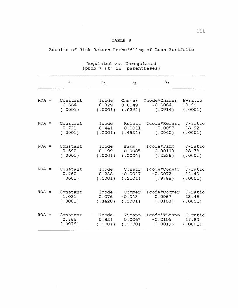
IllTABLE 9

Results of Risk-Return Reshuffling of Loan Portfolio

Regulated vs. Unregulated (prob > It| in parentheses)

ROA = Constant 0. 684 (.0001)

I code 0.329 (.0001) (.0244)

Cnsmer Icode*Cnsmer F-ratio 0.0049 -0.0064 13.99

(.0914) (.0001)

ROA = Constant 0. 721 (.0001)

Icode 0.441 (.0001) (.4534)

Relest Icode*Relest F-ratio 0.0011 -0.0057 18.92

(.0040) (.0001)

ROA = Constant 0. 690 (.0001)

Icode 0.199

Farm0.0085

(.0001) (.0004)Icode*Farm

0.00199 (.2538)

F-ratio 28. 78 (.0001)

ROA Constant 0. 760 (.0001)

Icode 0.238 (.0001)

Constr -0.0027 (.5101)

Icode*Constr -0.0072 (.9788)

F-ratio 14. 43

(.0001)

ROA = Constant 1.021

(.0001)Icode 0.076 (.3428)

Commer -0.013 (.0001)

Icode*Commer 0.0067 (.0103)

F-ratio 33 .48

(.0001)

ROA = Constant 0.365 (.0075)

Icode0 . 821 (.0001)

TLoans0.0067 (.0070)

Icode*TLoans -0.0105 (.0019)

F-ratio 17.82

(.0001)

112Therefore, it can be concluded that regulated banks did

reshuffle its.loan portfolio in two ways:1 . by increasing total consumer loans, as a

percentage of total assets faster than unregulated banks and

2 . internal reshuffling took place within real estate, consumer,and commercial categories, with a tendency to invest in higher-yielding higher-risk loans. Based on the results of Table 9, the overall tendency of this internal reshuffling was to invest in higher-yielding, higher-risk loans

The same yield-risk relationship is applied when interpreting the behavior of the investment securities portfolio. Traditional analysis would interpret increased investment in investment grade securities as risk reducing based upon the general perception of the default risk of the issuer. However, two facts preclude such a conclusion. First, of the three categories of investment securities in which banks actively trade, U.S. securities, agency securities and municipals, municipal securities are riskier in terms of default risk, for example, New York City and WPPSS bonds. And as shown in Table 8 regulated banks significantly increased the rate of investment in municipal securities during the post-regulation period. Secondly, by appealing to the arguments outlined in the discussion of loan portfolio reshuffling, the fact that regulated banks have increased their yields on' investment securities at a significantly (prob=.108) faster rate than the unregulated sample, may in turn imply an internal reshuffling of the

113investment portfolio. Even' though relative investment in investment securities has risen, it may be argued that in order for the regulated bank to earn significantly higher yields it must purchase riskier securities.

Thus, it appears that the results from Tables 6-9 provide evidence in support of rejecting the null hypothesis that changes in the asset portfolio characteristics of regulated and unregulated banks were insignificant. On the liabilities side, it was found that the regulated bank restructured its financing resources. As shown by Table 8 , the regulated bank relied more heavily on demand deposits as a source of funds. While this change was found to bestatistically significant its impact upon portfolio risk and upon default risk would be speculation at most.

In conclusion, based upon the univariate and multivariate tests there appears to be sufficient evidence to reject the null hypothesis and accept the hypothesis that in response to mandated capital regulation, banks will reshuffle their asset portfolio. This resultant post-regulation asset portfolio will be composed of more risky assets which could result in a higher probability of default for a regulated bank.

Additional Assumptions of the ModelIn addition to the basic assumptions of the

2classical linear regression model, i.e., e^ N(0,o ) and E(E^Ej)=0 , i*j/ the reshuffling test equation also incorporates an assumption regarding the variable YR. As discussed, the coefficient of YR from (59) is interpreted as the rate of change in a financial variable for the four years following capital regulation. However, implicit in the model's design is the assumption that this estimated change is uniform or equal change across the test period.45 For example, in reaction to capital regulation a bank may react sharply and make adjustments in the first year and remain at that position throughout the test period. In this case, the possibility exist that such an adjustment by the bank may be undetected by the original model due to a smoothing of information over the test period. That is, a significant reaction in period one may be washed out by similar behavior between the matched pairs in periods 2,3 and 4.

Thus, to test this uniformity assumption and to gain further insight into the adjustment process by regulated banks, the following regression was run:

45 See Kmenta (1971), pg. 413 for a discussion of this assumption.

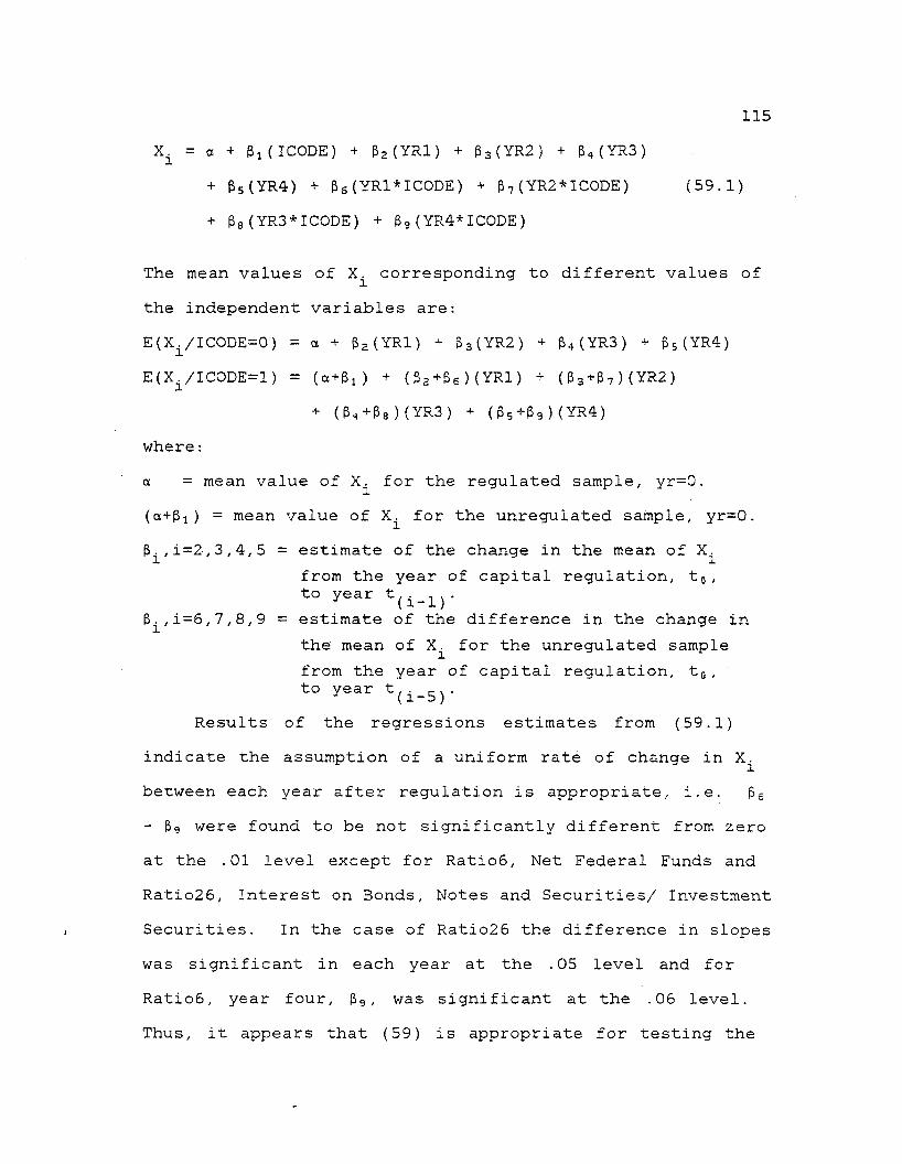
115X± = a + Pi(ICODE) + B2(YR1) + 3 3(YR2) + 34(YR3)

+ 35(YR4) + 3S(YR1*IC0DE) + p7(YR2*ICODE) (59.1)+ 3S(YR3*ICODE) + 39(YR4*ICODE)

The mean values of corresponding to different values of the independent variables are:E(Xi/ICODE=0) = a + fr2 (YRl) + B3(YR2) + B4(YR3) + 35(YR4) E(Xi/ICODE=l) = (a+Bi) + (32+36)(YRl) + (B3+37)(YR2)

+ (B^+B8)(YR3) + (B5+69)(YR4)where:a = mean value of X^ for the regulated sample, yr=0 .(o+Bi) = mean value of X^ for the unregulated sample, yr=0 .3^,i=2, 3,4,5 = estimate of the change in the mean of X^

from the year of capital regulation, t 0, to year t ̂̂ .

3^,i=6,7,8,9 = estimate of the difference in the change inthe mean of X^ for the unregulated samplefrom the year of capital regulation, t0,to year t , . . .J (1-5)

Results of the regressions estimates from (59.1) indicate the assumption of a uniform rate of change in X^ between each year after regulation is appropriate, i.e. 3s - 3g were found to be not significantly different from zero at the .01 level except for Ratio6, Net Federal Funds and Ratio26, Interest on Bonds, Notes and Securities/ Investment Securities. In the case of Ratio26 the difference in slopes was significant in each year at the .05 level and for Ratio6, year four, 3g, was significant at the .05 level. Thus, it appears that (59) is appropriate for testing the

116reshuffling hypothesis and, in addition, the reaction by banks to capital regulation followed a smooth rather than a jump process. Such a result may be expected if regulated banks felt that regulators were now monitoring their actions more closely. And that any abnormal activity by the bank may result in additional examination and regulation.

Default-Risk HypothesisThe second major hypothesis to be tested centers around

the relationship between asset portfolio reshuffling and probability of default risk. As shown by Swary (1980), Edwards and Scott (1976), and Koehn and Santomero (1980), the ability of capital regulation to alter default risk can be expressed both mathematically and graphically. Simply, additional capital can reduce the probability of default by providing a higher equity threshold from which bankruptcy is defined. The regulated institution which now has a greater cushion of equity to operate with will be able to withstand higher levels of operating losses and/or asset devaluations. As shown in Figures 2 and 3, increases in capital will result in lower probability of failure, holding other factors constant. The problem arises, however, when a regulated bank alters its returns distribution by reshuffling the asset portfolio. In particular, as exhibited in Figure 2 such a change in investment strategy

117could result in a risk-return locus which possesses default risk contrary to regulators intent. The empirical question then becomes, whether as a result of asset portfolio reshuffling following capital regulation, does the regulated bank improve or deteriorate its risk-return locus vis-a-vis an unregulated bank?

Using the same 79-bank sample used in the reshuffling tests, (62) was employed to measure the effect of assets portfolio reshuffling upon default risk for regulated banks.4 6

ROA = a + Pi (Icode) + $2(Risk) + fj 3 (I code*Ri sk)Introduced as portfolio risk proxies were:

1. Riskl= Coefficient of Variation of Net Income.2. Risk2= Variance of Return on Assets(ROA).3. Risk3= Coefficient of Variation of ROA.4. Risk4= Chebyshev's Inequality.

Average net income for the post regulation period, yr=l,2,3,4, was the dependent variable used as the portfolio return proxy regressed on Riskl. Average return on assets for the post regulation period, yr=l,2,3,4 was the corresponding return proxy associated with the other risk measures.

46 A similar application of this model is found in D'Antonio and Melchier (1979).

118Interpretation of the regression results follows that

of the reshuffling tests, where the coefficient of the interaction term f$3 represents the difference in behavior between the regulated and unregulated sample with respect to default risk. A significant positive sign for 3S would imply that regulated banks were increasing their probability of default faster than the unregulated sample over the testing period. A significant negative sign for the interaction term notes a reduction in default risk probability by the regulated banks relative to the unregulated sample.

The results of the default-risk hypothesis tests are given in Table 10.

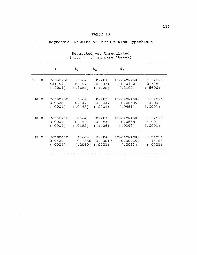
119TABLE 10

Regression Results of Default-Risk Hypothesis

Regulated vs. Unregulated (prob > |t| in parentheses)

NI Constant 431.57 ( .0001)

Icode 62 . 57 (.3668)

Riskl 0.0331 (.4128)

Icode*Riskl -0.0742 (.2104)

F-ratio 0. 694 (.5606)

ROA = Constant 0.9526 (.0001)

Icode 0. 147 ( .0148)

Risk2 -0.0047 (.0001)

Icode*Risk2 -0.00599 (.0468)

F-ratio 13.00

(.0001)

ROA = Constant 0.9007 (.0001)

Icode0. 142 (.0188)

Risk30.0439 (.1426)

Icode*Risk3 -0.0638 (.0398)

F-ratio4. 901 (.0001)

ROA = Constant Icode Risk4 Icode*Risk4 F-ratio0.9429 0.1556 -0.00019 -0.000394 16.68(.0001) (.0069) (.0001) (.0023) (.0001)

120Two significant conclusions can be reached from

the above results:1. For all risk proxies tested, the sign of the

interaction term is negative and three of the four coefficients are statistically significant, 33 <0. This implies that the unregulated banks v/ere increasing their probability of default relative to the regulated bank sample.

2. For two overall risk proxies, Risk2 and Risk4, the signs of the coefficients were negative, 32 <0- And, in addition, observing that (32 + P3) is negative for each regression equation implies a negative relationship between risk and returnfor the unregulated sample over the entire time period.

The fact that 33 was consistently negative would appear to be inconsistent with the results of the reshuffling tests. Where it was concluded that regulated banks were indeed reshuffling their asset portfolios investing in more risky assets. This did not, however, require a corresponding increase in the probability of default for such a bank. A reconciliation of these findings is provided from the additional result that these same banks were realizing higher return from investments and becoming more operationally efficient. Therefore as shown by the default risk tests, the net effect of both risk and return increases by the regulated bank sample has actually resulted in a higher return-risk locus, i.e., return is increasing faster than risk. This in turn implies a lowering of default probability by the regulated banks relative to the unregulated sample.

1 2 1

The second point addresses the issue of the "soundness" of the banking industry. A priori, a positive relationship between risk and return is expected, but such was not the case for the sample of banks in this study.. Instead the observed negative sign for &z and (fh + S3) both suggest that over the time period tested, the banking industry or a sector of the industry represented by this sample has become more risky, increasing its probability of default. Considering, however, the time period under study, 1972-1981, with its severe economic swings and volatile interest rates, such a result may be hardly surprising or unexpected.

In conclusion,, the results of the default-risk tests support accepting the null hypothesis that regulated banks do not increase default risk as a result of capital regulation. In fact, the impact of capital actually appears to result in a reduction of default probability and more efficiently managed commercial banks.

I

Chapter VI SUMMARY, LIMITATIONS, AND CONCLUSIONS

In order to understand the interrelationship between bank capital regulation and the decision-making process of a commercial bank, several models of the banking firm were analyzed and discussed. Ranging from Swary's constrained optimization framework to O'Hara's dynamic modelling, there is substantial theoretical justification to suspect that banks will reshuffle their asset portfolio in response to a regulated increase in equity capital. As a result, the bank will possess a riskier asset portfolio, which, in turn, may imply an increase in the bank's probability of default.

Empirical testing of the reshuffling hypothesis and the corresponding default-risk hypothesis was performed using a test sample of banks which, from 1972-1977, were ordered by regulators to increase their equity capital. Due to the small asset size of the banks forced to increase equity capital, no market price data were available for testing. Therefore, both univariate and multivariate testing were designed using a peer group (a sample of similar banks that did not experience a regulated capital structure shift) as a benchmark or control sample with which to compare and contrast the behavior of the test sample. Differences or similarities between these two groups were measured relative to various balance sheet and income statement ratios which

122

123served as proxies for asset' portfolio holdings and asset risk measures.

Results of the empirical tests provide tentative evidence that, in reaction to a regulated increase in equity capital, banks will reshuffle their asset portfolios and/or alter their profitability and operating characteristics. Specifically, it was found that, in contrast to the control sample, such banks:

1. Reshuffle their asset portfolio by increasing net balances of federal funds, increasing investment in municipal securities and consumer loans and increasing the use of demand deposits.

2. Significantly increase average yields on investment securities portfolio, return on equity and return on total assets.

3. Become more operationally efficient by reducing their operating expense to operating income.

Further, there is evidence that these same banks are internally reshuffling their loan portfolios. Under the assumption that higher returns imply increasing risk, the results of the loan portfolio reshuffling indicate a tendency for the test sample to make riskier real estate and commercial loans and, also, to increase the overall risk of the loan portfolio.

Finally, the default risk hypothesis was tested by comparing changes in the risk-return locus of the test and control samples. The resultant default-risk levels of the test sample were found to be decreasing relative to the

124control sample. Reconciliation of the reshuffling and default-risk tests suggest that any observed increase in portfolio risk by banks forced to increase equity is being dominated by the corresponding increase in operating efficiency.

Therefore, it appears that the effects of a regulated increase in equity capital upon the decision-making process of the commercial bank are two-fold:

1. banks will respond by reshuffling their asset portfolio selecting a riskier portfolio than would be expected, and

2 . banks become more operationally efficient,the net result being a reduction in default-risk vis-a-vis banks not subject to regulated increases in equity capital. Thus, if it is generally agreed that the objective of capital regulation is to improve the riskiness of banking system the evidence lends support to the premise that regulatory actions are indeed effective and successful.

The scope of the results is limited by sample characteristics and data constraints. As discussed in Chapter 4, the screening process for inclusion in the test sample yielded relatively small banks - average total assets of $34,000,000. Thus, the application of any empirical results to large banks is questionable. Also the possible shortcomings of the data base must be considered. First, the use of book values instead of market or economic values

125of the asset and liabilities variables for testing introduces possible valuation errors. Second, results based on only four years of data subsequent to the regulation and the absence of any pre-regulatory data surely restricts the power of the statistical models.

Much more work, both theoretical and empirical must be done in the area of capital regulation before its full impact on the behavior of the bank becomes clear. As the dynamics of the banking firm are more clearly understood, and as data becomes more accessible and accurate, further insights into the effectiveness and efficiency of capital regulation may be revealed.

i

126BIBLIOGRAPHY

Baltensperger, Ernst, "Alternative Approaches to the Theory of the Banking Firm", Journal of Monetary Economics, 6 : 1-37. June, 1980.

Baxter. N., "Leverage, Risk of Ruin and the Cost ofCapital", The Journal of Finance, 22: 395-403., September 1967.

Bentson, George, "Bank.Examination", The Bulletin, New York University Graduate School of Business Administration, Nos. 89-90., May 1973.

Black, Fischer, Merton Miller and Richard Posner, "AnApproach to the Regulation of Bank Holding Companies", Journal of Business, 51: 379-411., September 1978.

Blair, Roger and Arnold Heggestad, "Portfolio Regulation and the Probability of Bank Failure", Jounal of Money, Credit and Banking, 10: 88-93., February 1978.

Board of Governors of the Federal Reserve System, Report of Income and Report of Condition, April 1979.

Cargill, Thomas and R. Meyer, "Dynamic Portfolio Behavior of Commercial Banks: An Intergrated Analysis", Quarterly Review of Economics and Business, 22: 67-80., Spring 1982 .

D'Antonio, Louis and Ronald Melchier, "Changes in Federal Reserve Membership: A Risk-Return Profitability Analysis", The Journal of Finance, 34: 987-997.,September 1979.

Dothan, Uri and Joseph Williams, "Banks, Bankruptcy and Public Regulation", Journal of Banking and Finance, 4: 65-87., September 1980.

Edwards, Franklin and James Scott, "Regulating the Solvency of Depository Institutions: A Prespective for Deregulation", Issues in Financial Regulation, 1978, 65-122.

Goodman, Laurie, "The Bank in Insolvency: Regulatory Decisions and Economic Values", National Bureau of Economic Research, Working Paper no. 187, August 1977.

Guffey, Roger, "After Deregulation: The Regulatory Role of the Federal Reserve", Economic Review, Federal Reserve Bank of Kansas City, 68: 3-7., June 1983.

127Gujarati, Damodar, "Use of Dummy Variables in Testing for

Equality Between Sets of Coefficients in Two Linear Regressions: A Note", The American Statistician, 24: 50-52., February 1970.

Gilbert, Gary, and Manfred Peterson, "The Impact of Changes in Federal Reserve Membership on Commercial Bank Performance", The Journal of Finance, 30: 713-719., June 1975.

Hart, Oliver, and Dwight Jaffee, "On the Application ofPortfolio Theory to Depository Financial Intermediaries", Review of Economic Studies, 41: 129-147., Janurary 1974.

Heggestad, Arnold and B. Frank King, "Regulation of BankCapital: An Evaluation", Economic Review, Federal Reserve Bank of Atlanta, March 1982.

Howard, Donald, and Gail Hoffman, Evolving Concepts of Bank Capital Management, Citicorp, 1980.

Jacobs, Donald, H. Prescott Beighley and John H. Boyd, "The Financial Structure of Bank Holding Companies", Trustees of the Banking Research Fund Association of Reserve City Bankers, 1975.

James, John, "Portfolio Selection with an Imperfectly Competitive Asset Market, Journal of Financial and Quantitative Analysis, 831-846., December 1976.

Kahane, Yehuda, "Capital Adequacy and the Regulation ofFinancial Intermediaries", Journal"of Banking and Finance 1: 207-218., 1977.

Kane, Edward, "The Capital Adequacy Card Game", The American Banker, 5-9., September 18, 1981.

__________ and Stephen Buser, "Portfolio Diversification atCommercial Banks", The Journal of Finance, 34: 19-34., March 1979.

Klein, Micheal, "A Theory of the Banking Firm, Journal of Money, Credit and Banking, 33: 205-218., May 1971.

Kmenta, Jan, Elements of Econometrics, MacMillian Publishing Co. Inc., 1971.

Koehn, Micheal, and Bruce Stangle, "The Effect of Deposit- Rate Ceilings on Bank Risk: A Comment", Journal of Banking and Finance, 4: 381-386., 1980.

128______ , Bankruptcy Risk in Financial Depository

Intermediaries, Lexington Books, 1979._____ , and Anthony Santomero, "Regulation of Bank Portfolio

Risk", The Journal of Finance, 35: 1235-1244., December 1980.

Lam, Chun, "Bank Holding Behavior and Effectiveness of Capital Regulation,' Working Paper no. 131 Tulane University, August 1978.

Luckett, Dudley, "Credit Standards and Tight Money", Journal of Money, Credit and Banking, 2: 420-434, November 1970.

Maddala, G. S., Econometrics, New York: McGraw Hill Book Co., 1977.

Maisel, Sherman, and Robert Jacobson, "Interest Rate Changes and Commercial Bank Revenues", Journal of Financial and Quantitative Analysis, 687-700., November 1978.

Mayne, Lucille, "Supervisory Influence on Bank Capital", The Journal of Finance, 627-651., June 1972.

Mazzoleni, P., "The Influence of Reserve Regulation and Capital on Optimal Bank Asset Management", Journal of Banking and Finance, 1: 297-309., 1977.

Meinster, David, and Rodney Johnson, "Bank Holding Company Diversification and the Risk of Capital Impairment", The Bell Journal of Economics, Autumn 1979.

Meltzer, Alan, "Major Issues in the Regulation of Financial Insitutions", Journal of Political Economy, 24: 482-500., August 1967.

Merton, Robert, "An Analytic Derivation of the Efficient Frontier", Journal of Financial and Quantitative Analysis, 1851-1872., September 1972.

Michealsen, Jacob and Robert Goshay, "Portfolio Selection in Financial Intermediaries: A New Approach", Journal of Financial and Quantitative Analysis, 166-199., June 1967.

Mingo, John, "The Effect of Deposit Rate Ceilings on Bank' Risk", Journal of Banking and Finance, 2: 367-378., 1978.

___________ , "Regulatory Influence on Bank CapitalInvestment", The Journal of Finance, 30: 111-121., September 1975.

129_________, "An Imperfect Markets Model of the Banking Firm

Under Regulation", Research Report, Division of Research and Statistics Board of Governors, Federal Reserve System, 1977.

_________ and Benjamin Wolkowitz, "The Effects of Regulationon Bank Balance Sheet Decisions", The Journal of Finance, 32: 1605-1616., December 1977.

Neter, John ,and William Wasserman, Applied Linear Statistical Models, Richard D. Irwin, Inc., 1974.

O'Hara, Maureen, "A Dynamic Theory of the Banking Firm", The Journal of Finance, 38: 127-140., March 1983.

Orgler, Yair, and Benjamin Wolkowitz, Bank Capital, Van Nostrand Reinhold Company, 1976.

Ostle, Bernard, and Richard Mensing, Statistics in Research, The Iowa State University Press, 1975.

Peltzman, Sam, "Capital Investment in Commercial Banking and Its Relationship to Portfolio Regulation", Journal of Political Economy, 1-26., January/February 1970.

Pettway, Richard, "Market Tests of Capital Adequacy of Large Commercial Banks", The Journal of Finance, 31: 865-875., June 1976.

Porter, R. C., "A Model of Bank Portfolio Selection", Yale Economic Essays, 1: 323-335., Fall 1961.

Posner, Richard A., "Theories of Economic Regulation", Bell Journal of Economics, 5: 335-358., Autumn 1974.

Pratt, J. W., "Risk Aversion in the Small and the Large", Econometrica, 122-136., June 1964.

Pringle, John, "A Theory of the Banking Firm", Journal of Money, Credit and Banking, 990-996., November 1973.

_____ , "The Imperfects-Markets Model of Commercial BankFinancial Managment", Journal of Financial and Quantitative Analysis, 69-87., January 1974.

_____ , "The Capital Decision in Commercial Banks", TheJournal of Finance, 29: 779-795., June 1974.

Pyle, David, "On the Theory of Financial Intermediation",The Journal of Finance, 26: 737-747., June 1971.

130_____ , "Descriptive Theories' of Financial Institutions Under

Uncertainty", Journal of Financial and Quantitative Analysi s , 2009-2029., December 1972.

Quandt, Richard, "Tests of the Hypothesis that a LinearRegression System Obeys Two Seperate Regimes", Journal of the American Statistical Association, 324-330., June 1960.

Ratti, Ronald, "Bank Attitude Towards Risk, Implicit Rates and the Behavior of an Index of Risk", The Quarterly Journal of Economics, 309-331., September 1980.

Reed, Edward, Richard Cotter, Edwars Gill, and Richard Smith, Commercial Banking, Prentice Hall Inc., 1980.

Robinson, Roland, and Richard Pettway, "Policies for Optimum Bank Capital, A Study Prepared for the Trustees of the Banking Research Fund, Association of Reserve City Banks, 1967.

Rosenburg, Barr, and Philip Perry, "The FundamentalDeterminants of Risk in Banking", Proceedings from a Conference on Bank Structure and Competition, Chicago: Federal Reserve Bank of Chicago, 1978.

Ross, Stephen, "The Arbitrage Theory of Capital AssetPricing", Journal of Economic -Theory, 13: 314-360., 1976.

Roy, A. D. , "Safety-First and the Holdings of Assets", Econometrica, 431-449., July 1952.

Santomero, Anthony and Joseph Vinso, "Estimating the Probability of Failure for Commercial Banks and the Banking System", Journal of Banking and Finance, 1: 185-205., 1977.

___________ and Ronald Watson, "Determing An Optimal Standardfor the Banking Industry", The Journal of Finance, 32: 1267-1282., September 1977.

SAS Users Guide: Statisties 1982 Edition, Raleigh, North Carolina: SAS Institute Inc., 1982.

Sealey, C.W., "Deposit Rate-Setting, Risk Aversion, and the Theory of Depository Financial Intermediaries", The Journal of Finance, 35: 1139-1154., December 1980.

_____ and James Lindley, "Inputs, Outputs, and a Theory ofProduction and Cost at Depository Financial Institutions", The Journal of Finance, 32: 1251-1266., September 1977.

131Scott, James, "The Probability of Bankruptcy", Journal of

Banking and Finance, 5: 317-344., 1981._____ , and Franklin Edwards, "Bank Solvency Regulation in

the United States: A Theoretical Analysis", Working Paper No. 87A, Graduate School of Business Columbia University, July 1977.

Sharpe, W. F., "Bank Capital Adequacy, Deposit Insurance,And Security Values (Part I)", National Bureau of Economic Research, Working Paper 209, October 1977.

Sinkey, Joseph, Jr., "identifying Problem Banks", Journal of Money, Credit and Banking, 10: 184-192., May 1978.

_____ , "A Multivariate Statistical Analysis of theCharacteristics of Problem Banks", The Journal of Finance, 30: 21-36., March 1975.

Silverburg, Stanley, "Deposit Costs and Bank PortfolioPolicy", The Journal of Finance, 25: 881-895., May 1970.

Swary, Itzhak, Capital Adequacy Requirements and Bank Holding Companies, UMI Research Press, 1978.

Taggart, Robert and Stuart Greenbaum, "Bank Capital andPublic Regulation", Journal of Money, Credit and Banking, 10: 158-169., May 1978.

Talmor, Eli, "A Normative Approach to Bank CapitalAdequacy", Journal of Financial and Quatitative Analysis, 15: 785-811., November 1980.

Telsler, Lester, "Safety First and Hedging", Review of Economic Studies, 23: 1-16. January 1955.

Vinso, Joseph, "A Determination of Risk of Ruin", Journal of Financial and Quantitative Analysis, 14: 77-100., March 1979.

Vojta, George, Bank Capital Adequacy, New York: Citicorp 1973 .

Warner, J., "Bankruptcy Costs: Some Evidence", The Journal of Finance, 337-347., May 1977.

Whitehead, David and Robert Schweitzer, "Bank Size and Risk: A Note on the Evidence", Economic Review, Federal Reserve Bank of Atlanta, November 1982.

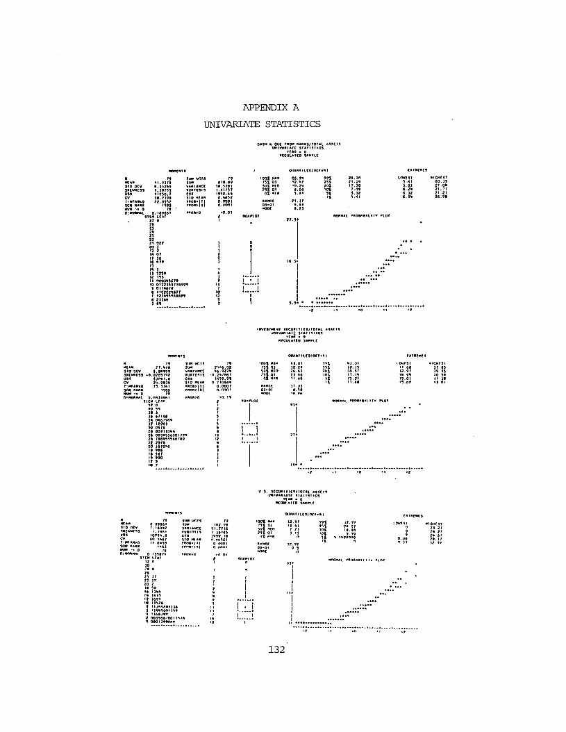
APPENDIX A UNIVARIATE STATISTICS

CASH ft OUC 7*0*1 RARHS/T01AL ASSETSu n i v a r ia i c s t a t i s t i c s

VtA ft > 0■ c cu L A tfO sam rlC

MfARS IO K V JK U H C SS MSSCVT'H fAIN O SCH AAMR RUM •« 0 9 : wqrkal

T9I I . 1378 f t . J 12991 . 1 9 m 1 1 2 5 9 .7 1 0 .7 1 9 0 7 2 .9 3 3 2

1900790. 109001 311" LCAT

I T 0

Si m w i t s5UHVAftlARCC KURfOSIS CSSSTO MtAR R * O 0 » jl | r ro r* I s i

*R08>0

79 100 1 MAX 2 0 .9 80 7 9 .0 9 751 01 12 *7

1 0 .9 9 0 1 5 0 1 MtO 1 0 .2 ft1 .0 1 7 3 1 2 3 1 Ql 0 .0 01 * 9 0 .0 9 0 1 RIR 5 .0 10 - 0 0920 .0 0 0 1 RANGE 2 1 .3 70 .0 0 0 1 Q 3 -0 I f t .f t l

MOOC 0 . 2 )

QUART11(91 OCT• A1m93%901101

1 7 .9 0 7 .0 9 S . 32 9 .0 1

LOWCSf3613 .9 10 .2 f t0 .3 20 .3 f t

RORMAL ARO0ADILIT

HlCMCSt2 0 . J3 2 1 .0 f t2 1 . 17 2 1 .2 1 2 0 .9 0

21 22 21 0 2 2 2 0 1 19 2 10 07 17 3010 * 7 9 131ft 711 2 2 9 012 19911 0 0 0 3 * 9 0 7 9 10 O I2 2 3 3 3 7 7 0 0 9 9 9 0 1 1 * 0 7 9 • 11 2 2 2 2 * 0 7 7 7 1 2 3 * 9 9 9 0 0 0 9 9 0 23 3 0 0 3 0 9

•MVCSTMIRI S tC U R IIIC S /rO IA L A 99C19 UR I VAR I A IC STA TISTICS

» fA * I 0 RCCULAltO 3AMRLC

Q U A R TILCSfO ft**}

M<AR SIO o t v s a c w R ts s u s *CV1 Mf AM«0 SON RARR RUM •» 0 O'RORMAL

797 7 .* 1 0

0 .0 * 9 9 9 •0 .0 2 0 9 7 * 7

0JO W 7.0 2 9 .9 0 3 0 3 9 -9 7 0 1

1980 19

SIM WR7S SUMVAR1ARCC HUN 10*1S CSSSIO MfAR * * 0 8 * I 1 I RROR*IS I0. OR] 1 ftA1

SICM L fA l *2 0 *0 3*30 330 0 7 1 0 0 3ft 0 * 0 7 9 0 9 32 12903 3 0 0 9 7 9 2 0 0 0 1 1 3 3 * 0 2 0 0 0 3 * 9 3 0 0 0 1 7 9 9 2ft 7 0 9 * 0 9 9 0 0 7 * 9 22 2 079 20 3070 9 0 ■ 0 9 9 0 10 9 0 7 Ift 9 0 0 12 0 10 7

f«<TR»0

792 1 0 0 .0 2 * 0 .9 2 2 *

O .2 4 /A 0 1 1 0 9 9 .9 9

0 .7 7 0 0 0 * 0 .0 0 0 1 0 . orx>«

>0. 19

*00 1 HAR 731 03 3 0 1 M tn 2 9 1 Ql

0 1 RIR

* 3 .0 1 3 2 .2 9 2 0 .0 3 23 00 1 I 00

3 1 .3 39 .9 9

1 0 .0 0

S * !9 9 19 0 1"01?1

* 3 .0 1 3 9 . 19 3 0 .0 7 1 7 .7 * 1 9 0 1 1 1 .6 0

1 2 .9 7 1* . 991 3 .0 11 9 .0 2

RfCRrsi 3 7 .9 9 3 9 . 39 * 0 .9 *

RORMAL RRORAI

U .S . 3CCW M11 (9 7 1 0 7 A t A 9 S (I9im tV A R iA tc s t a t i s t i c s

v (A * • o RCOU IA ltO SAMRtt

« 7 A R t l t C S m i < f t |

MTARSIO o c v9N(WMf*3u s *

790 .0 9 0 0 11. 100*2

1. 19A I 1 0 2 9 * .0 0 0 .* 0 0 7 11 0*9 0

1*03 10

0 13907* SU M L IA f

32 R

SIM WRI3 9t7MVARIANCE ■ U R I09 I9CSSS t o MfAR W 1O 0»|1 I r R o R * u |

797R 2-99

9 1 .2 7 1 0 l . 39103 3 9 9 9 .1 0 0 .* 0 9 0 1

9 .0 0 0 1 0 n o n I

• 0 0 t mar 191 Ql 5 0 1 »tf> 2 3 1 Ql

1 2 .9 7 1261 7 .2 1 3 1)

99 195 19 0 1'?}

1%

3 2 .9 7 71* 27 1 0 .9 0 0 .9 9

i 0 9 9 9 * 9 9

MlCMfST 2 3 .2 1 2 f t .27 2ft 0 7 29 . 77 1 7 .9 7

RORMAL 7RORARII I

207* 37 22 2?2 0 2 I* 90 10 l i f t*I * 3*39 12 3091 10 33*20 0 1 1 3 * 9 0 0 1 )3 0 0 11**9 0 0 1 1 9 9 • 1 )0 0 7 9 9 2 0 0 )9 0 0 7 0 0 1 1971 0 0 0 0 I 3990R9

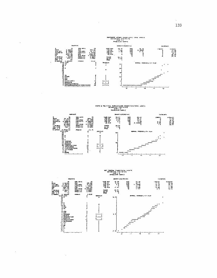
133

m ? A t M V I 1

c u t A r r o s a n a i r

m .* *SIO o t v

u s sCVI t M t l ' O SOU MANNRUM — 0 O'NORMAl

S l fHJO

795 5 6 0 / S S . f 9 0 6 6 2 . t M R / 6 0 5 / . 3 6

1 2 1 .6 0 7 .) 0 * S 6

IO I 7 .5 65

0 . 20S 8A / U A »5 /

StIH 1*11 S SUMVAAIAMCtKURIOSISCSSSIO - t* R M 0 8 > l M 7 n n n * M l

PR0R»0

79«*io. so’*6. i n

5 . J 5 I 9 6 1 5 9 6 .a ?

o . t t u n o i o .o o o i n .n n r n

' 0 . 0 1

100% HA* JO. 7*'5% Q) 7 .6 *50% Nff> 2 .1 5>5% 01 1

0% MIR <1

RAmCC j o . ;*0 3 -0 1 6 . A*►*>07 n

99%96%90%

uKursr * 1 .5 6 ? J . 1 9

2 * . 9 1 0 .9 9 JO . /9

t 0 /8 * 9 I 9 5 )I 999I 0 1 1 1 /1 ) 5 6 7 /I 66099969 ! 0 1 5 ) 9 6 6 / 7 / 9 0 ? ) )I 0 0 0 0 0 0 0 0 0 0 0 0 0 0 9 9 9 /9 0 0 0 1 9 6 9 9 9

II

- ? •0

S I A t t 6 R H lH C A l 9I/90IV ISIO M S SICURI » U S / * 0 1 Al. M S fT J URIVAR IA I% S / A I 'S / I C S

VfAR ■ O■ C C taA K O 5AM71 f

Qt/AMMICSI 0 7 7 - 9 1

MCA*s / o o t vU ( W ( »u s sCVT: M7 AN-0 SUM RANK RUM •« 0 OtMORMAI

/91 0 .1 6 1 9 5 .5 0 /1 9

0 .6 9 6 6 1 * 1 0 9 5 5 .a 5 * .0 6 9 5 * 6 .9 ) ? *

* 5 0 1 .5 //

SUM WOTS SUMVARIANCCa u m o s i sc s sS 'O " M RW 108»IMR * 0 * » 1 S |

7 * 0 0 * 0

199 0 9 . S I

5 0 . J5 0 6 O .9 6 0 8 9 9

2 ) 6 9 . 6 0 .6 1 9 6 2 *

0 .0 0 0 1 0 .0 0 0 1

* 0 . 15

t o o l HA* 75% 0 ) 50% M(0 25% 01

n% m i*

RAM6C0 5 - 0 1Moot

2 6 . 0 /l) .< J69 . " /

6 . *

99%99%901

2 8 . 0 / 16. I I * 6 - 9 1

* 0 9

m c w s rI 7 .9 2 1 8 .5 1 2 2 . 19 2 5 .6 9 2 8 . 0 /

■MMNAt. 7 * o n A * ll< T v 7 1 0 /

20 16 )16 1219*189 1* 1 2 * 91257 I ? 5 9 0 0 2 * 5 10 I2 M 5 5 5 6 U 5 N 9

1 1 ? S ? 2 )* * 6 96 1 1 )1 1 5 /6 1 2 2 6 * 6 • 111 1*1*662 960 0 0 * 9 *

R f 7 7 ( 0 t« A l /IIR O S/IO IA L *• UWtVA*1 A l t 51 At 1*1 ICS

yf A* • 0R fC U lA /rf t SAM71 f

01/AM f I L t 51 O t 7 - * 1

Mt ANS / o o c vI M W f S Su s scvf * MfAR-0 SRH AAN* RUM - • 00 ! RORMAl

792 .* 0 ) 5 * * .1 0 5 1 2

0 .* 7 9 6 ) 6 I9 Q 2 .0 * 1 / 9 . 1 15 1 9 6 2 2 /

a m . 5 r )

0 . 102**6 S 1 l » IIA 7 16 9

SUN u r n sSUMVARIANCC* 0 * 1 0 5 1 5CS6S t o M(A* 7 * 0 6 » I 11 7 * 0 « M S »

7R0*»O

191 6 9 .6 6 * 6 .5 1 *

I . ' 5 ) ) / 1 * * 8 .6 8

0 . * A * )6 ) 0 .0 0 0 1 o .o o o i

0 . 0 ) 9

AAM6C0 5 -0 1MOOt

» 6 .5 * * .* * 2 2

0. / 91

2* . 51

99%95%90%

• 5 . 75 - 5 .6 6

- * 5

MORMAt. 7 * 0 * A * I( .I?V 7 (0 1

H . *6 I I . 99 18. 5*

10 01 9 2 5 6 6 2?/6 *865 0 2 2 « 2***66*) 0 2 ) 6 / 9 2 2 7 * * * 9 5 /1 * 9 I 0 ) 5 5 /7 9 0 2 5 6 6 /7 7 /9 9 9

• 0 96IOOOOOO - I m •2 /)• ) 06

* 5 •5 11

■2

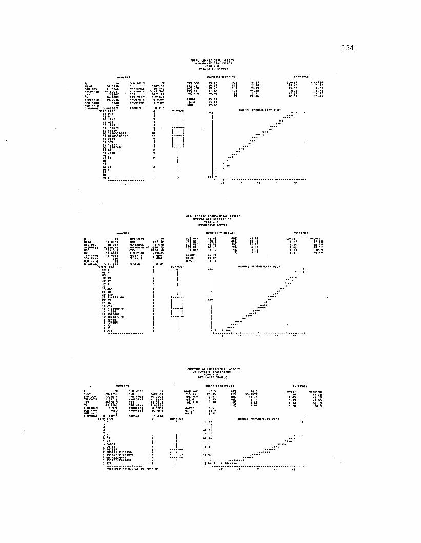
1 3 4

•OIAI LOAN3/tOI*l *13113 UNIVARIAIC SMIIItlCS

r?AR ■ 0r c c u i a u o sa m r i c

n * a sio ocv3RIVN79SUSSCVr*HfAR«0SCR RANKRUN •• 0 O'RORHAi

I f9 8 ,0 9 3 4 f . 16866

• 0 .6 0 0 J 1 27)907 I I . 1600 1 1 .9 9 0 6

'9 8 0 I f0.000001?

SU M U A I i* u ? r 12 9 IQ I t * '4 9 0 ) 6 66 144061 t9 9 4 7 R6 2 5 5 5 1 ?6 0 2 6 0 4 5 3 6 6 7 7 54 0 1 4 * 3 0 4 4 * 0 ? 36 217 3 3 » 3 5 9 32 37 6 7 7 30 1 2 3 6 7 8 )64 69 6 6 1 ) 3 8 66 2 62 R2 60 39

su n w o tsSUMVARIANCC nun m s i s CSSS t o NfAN 7808*I II ARON*1117*08*0

6369,56 40. 167

0.6)1061 6673.66 1 .0 3 6 ) | 0 .0 0 0 1 o.noot

0 . 1 16

QUANIHtSIOC?*11 7818CH7S

1001 MAR 79.47 991 19 67 10V7Sf191 0) 66. 9) 951 72 74 79. 06301 Mtn 39.42 9<>1 70- 13 13.80791 01 31 )Z 101 *4.20 JA.2

n t m in 29. 0A 91 17.91 17.91• 1 29.06 47.8)

0ANOC 49 41qi-ot 11.21MOOC 59.*2

4ICHCST 71.46 17. 79 73.96 7*. 16 73 67

NO*MAI. PRORARII 11

RCAl CStAtC LOANS/707AL ASSCIS UNIVAR IAt C SIAIIJtlCS

Vf AN • 0 RtCIAAfCO SAMRLC

OVANTItCSI0C7«* t

H(A*sto ocvSKWNfSSUSS

79•7.9147 10.277

0.4309R6 33)13.6

cv 37.6821IlNfAR.O 13.6099SCR RANK i960RUN 0 790:NO*N*t 0. 11 79<3

S U M It AC II 9

) • 46 19 491* 6 J230 469 74 90 2 6 0 ) 92 6 I I I 7 8 I I A 9 2 2 79 7 0 36 14 23916 1113 6 8 9 7 9 16 7 1 )9 8 12 4 9 7 6 6 6 9 10 1491 6 7 7 7 8

9 3 )6 6 4 6 <29909 6 3 )2 t )

SIM WOfS SUMVARIANCCKURfOSISCSSSTO MCAN PNO0>111 P*OR»!Sl

191607.32 109.619

•0.0)60179 92)4.18 t. 15624 0 .0 0 0 1 o.ooot'0.01

loot MAN 731 0) 301 MCO 731 01 ol MIR

RARcrOJ.QIm e z

O 7)9

6 5 .6 9 26.4 • 6.09 • 0 .1 5

16. 77 • 6.09

1 .1 7

991991901•0 131•1

69.89 30 . '4 11.46

6 . I I

mC'irST 17. 94 38. 74 19.37 62.4 69 *9

NONHAi M08ABIII1V PLOT

CINMCNCIAl tOARS/fOlAt A9SC73 UNIVARIA f C SIA7ISIICS

< C « • 0 •CGUIAI7D SAMPLC

Q U A N ii t r s ( o c r « 6 i

■CAN»10 ocv• K W f S SUS1

I f70.J 79 I I?.9416 '.31718 49900.2 6).AI6J•1.977

• 900 19

SIM W C MSUMVARIANCCIURI04IS CSS310 **C AN »R 0 8 » ( 11 fAON*I 91A80N»0

79• 6 0 9 .6 ) 1A 7 .9 9 9 I . 1 6 0 1 1 1 1 1 0 ) .9 » .4 5 0 2 0 0 -0 0 0 1 0 .0 0 0 1

o oio

• o o f MAH 111 Q) ) 0 | MCO 7 3 1 Ql

0 1 " • *

AANCC03-01mooc

1 0 .5 76 99 17 97 • 0.99

7 0 .5 1 19.9

15 97

991931901

■a70.3

"9.749916. 38

lo w e s t I 99 2 .0 5 4 3 . 79

49.01 3 0 . 13

1 4 .9

NO*MAI. RNONAR 11.1IV PIOT

4 69 4 011 46 6 4 ?) 0 0 1 ) 32 5 6 7 7 8 9 7 0 0 0 1 1 1 1 2 1 ) 1 )4 *1 3 3 9 6 6 7 7777 0 8 4 9 6 I 0 0 1 1 2 2 2 4 4 6 6 0 3 5 9 6 7 7 1 1 8 8 0 8 9 9 0 726

H U tt lP f * SU M . i f Af 9V <0

6 2 . 3»

' I47 . 9*

I) » .9 »

I• 7 9«

I7 .5 * '

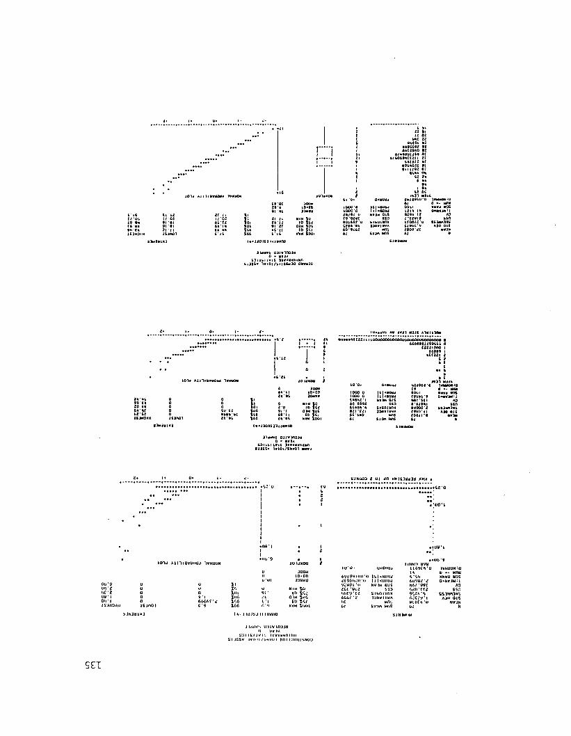
><V9l*0*i 1 * **0*

( 2 * 0 t 19 9* t ( '» ■

1 / 12 1/ o/Bi 61 91 91 21 i ti s j a o i

ec /• w '026i XI 6*’l* (6 **Ci(

!;.t o tt ut 6 6

IV Of 29 6 ftl *[21 11 2b 12 91 2 f *6 I f

1... i

«OUHi t - r b30M99

HIM ( 0ID i n 0)« tOt f b 1 6 / mr* too i

6 i o«

lt*00 0 lOOO'O 2 * / Bi 0 (9*02VC 6 0 1 6 9 2 '0 (296’6* 6 0 * 9 1 6 2 61

0< 909<

1 (1 < 9 0 * 4 111<90*6 H»6m O K

SCO d k u i a n i 33M9IVVA MAS S lIM MIS

< *1 22 Bi 11 02

9*1 22 9 9 (0 1 *2

6 * B t (0 2 *2 6 * 1 2 6 * 0 12

6 1 * * 6 6 1 1 6 * Of 6 l 6 0 6 9 * f ( 2 l I 2 f

6 * 1 6 ( 2 • ( 9 9 6 * 6 2 0 9 ( 9 1 1 1 /9 2 o r96** O*

62 2*6 kk

9* i •«62 06

<*11 M ) i ( 2 9 1 2 9 6 0 * 0 6/06*1 121* I*6 2 9 * 12 1 * (2 9 1 9 l ( 0 0 1 2 'o 6 1 9 6 6 V 1 6 0 9 '2 t61

0 • - MMf *■ 9* M9S o « i r * i9 : i

AO *66 KlMXt A )0 O K

■ 9 j9

I *»< JO I t 1 M 1*9/10

1 )<MV* U IJ9 1 A 0 2 *0 • NVJAS 3 I 1 * 1 | 9 | S 3 1 9 1 8VA1M/1

S l J S t * 1 * 1 0 1 /* ! 1 ( 0 * 3 0 0N9M10

AB 1 911 M ilh A U l i

2* *6 99 * 1 * 20 I*6* 9(12 62 IS lH O lH

I9W0M 1 9 * 9 0 9

Co ' £2 9 6 9 * *91 2* * 9 6

aooMI D - ( 030 * 9 9

"lb ?62 0)M lOt ( b 1 6 /

K9M to o I

1 0 0 *

1000 0 1000*0 (*6*2 * I 6 6 ’ (0 9 6 66V 6* * * •21*(2i6 6 * 6 9 961

0 « 9 0 M

I S | *0092 111 <8092 mv3m O K

s s oS 16019/1* 3099IMVA

MAS S lp f t MIS

C222IOOO |6 6 9 6 9 I *((221 I 6 2

9 I (*1 9 fe

9 6 < 9 ) 1 M i l t

* 2 1 0 ( 2 * 0 IVMtfONiO( 9 ( MM6001 BM99 K K(9 6 * 6 * 9 0«MV3tf‘ l9 6 1 * 6 (1 9 ’6 /6 * 1 6 V 0 0 0 ‘2 (9 6 0 * 1 1 1 0 2 1 1 * 9 61

(SO ( t ) M l l l

A30 O iS

t* > J 3 a iE ) l t lM 9 / iD

) ) * » • ( O JiV V tO )*0 ■ 99 )A

S O i l t l t V K 3 J 9 199AIM/I S 1 3 S 6 t l* 1 0 l/S M 9 0 1 M 09I

S J H U 0 3 2 0 1 2/1 J M J S 3 U 2 J 0 A9K •

J O l J A l l l l U V U i lU J 1VHUON

O o * 9on*2I l f *2 09 * I 00* 1 J S l i l l ) III

0l S J n o i

VI666/>f * 6*51

3 iXC otot yi*too ,;ir166 ‘.*11 6 6 m i

I V I H l b J I t INVJIO

3Q0Ht o - r nJ3I/VU

N IH 10 I t ) lit

0 1 H tO C fb V.t KVH tO O l

yzooi *ii 2 6 [ * 0 1 2 Miiyie 666/*2

WV IN O IS S S 3 SISOIMOM

3:>NVIUVA

f i 6 y f i ) * o i v h u o v o(ti 4*09 6U ‘/8 2 * 29 6 / * o e tWOtlZ 9 fj 2 i 'S 6 2 C / V 1 0 1 0 ( 9 * 0 61

U -*XNOU NOS 0»hvjh:i

A 3 S S .l

S S lH rtiM S A 'iO O IS NVJH

I i i i u v s t n i v i n o t uII 119 |A

S.*) I I S ! I VI (. 1 1VI HVAI III)S I J S S V I* | i 11 /S N V ll I n o t U l i l l lS N O J

sex

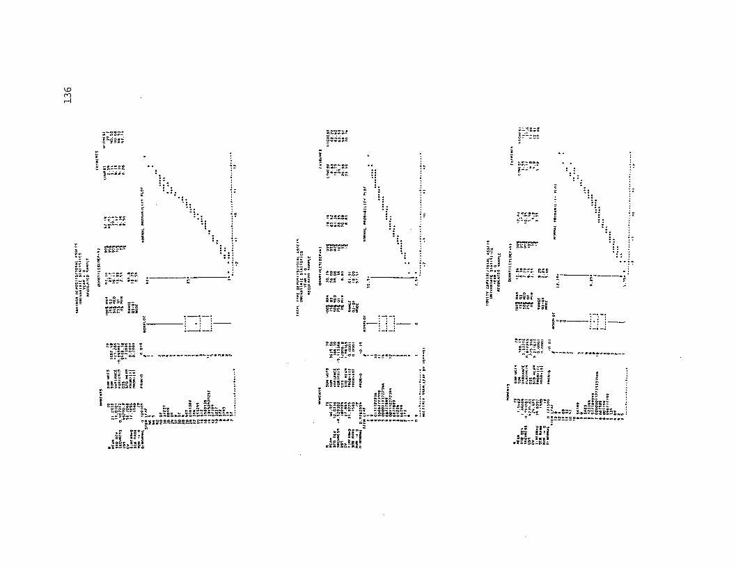
K D CO r —I

5S32SE

; 5£==2K

52-55*sr"'̂

L . 5 S B *

lit I !-5:

is* *c*S-« £“ILI L

PI ^ i | ! S i m

i l l i

*1:

;:i - : *ii

•;-£

■ □ 3 —

“SSSSSSSSSSgSSKilsiites

slEll

S3S~St

:2S£g£ fssisse* !!

!.|s 1 I

; SSS« gg;= ■-' r

p IslsiS III

I'

I I ! I

S III

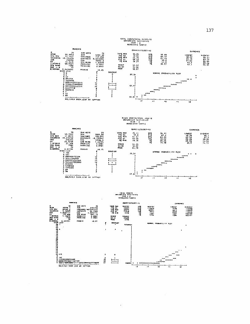
137j o t a l L O A N s / io f A t n r r o s i r s

UN I VAR I AT£ 6 I A I I S 7 I C S YEAR “ u

ftCG U LA U O SA H H £

MEAN S IU O tV SKIWNCSSu s sc vT :M C A N -0 SON RANKHUM *« 0 0 : NORMAL

7966. io5) 11.7U12 - 0 . 1 'i*>228

355*776 1 7 . 7 0 IN 5 0 .0023

1 5 0 0 79

s u m w a r sSUMVARIANCEM IM IO S ISc s sS IU MEANp n o n > { 11 r w m > i s i

0 .f l i i3 l> 2 5 3 SIC M LEAP

9 0 9 0 A 616 om?3h7 5 6 6 A 9 9 ?7 0 0 0 1 I I ? ? | J J 3 J » ,6 5 5 5 6 6 /7 7 a A 0 0 9 9 6 0 0 1 1 2 2 2 ) 3 3 3 ) j i | 5 6 0 6 7 7 7 / 9 5 0 0 0 0 2 J 9 •* 1 9 I I

A R nn> o

795 2 2 2 . 3 2 U 7 . 6 9 6

O .U V 9 3 V 6 '! 1 0 7 9 2 .n I .3 2 U 9 9 o . n o o i o . o o m

>0.15

l o o t MAX 75X Q3 5 0 X MCI) 2 5 t 01

O t MIN

RANOfQ 3 -Q IM oor

QUAMT I LF S( OET* 'I |

99%9 5 t90%» u t5%

IX

9 5 . 6 9 7 2 .9 1 6 6 . 75 9 6 . 59 36 2 7

5 7 .5 71 1 .3 23 0 .2 7

9 5 . OR l o w e s t8 5 . 72 3 8 .2 70 1 . 2 0 3 9 . 15

5 0 . 2 N 1 .0 39 1 . 2 '1 1 .2

3 0 . 2 7 '1 7 . 1

NORMAL PR O B A B IL IT Y PLOT

MIGHT ST 8 1 .2 1 8 5 . 72 00.66 0 9 . 6 6 9 5 . 0 9

M U LTIPLY S IE M .L C A f BY I O * « M lt

R ISK Y A S S T IS /I O I A I A S S M S i m i v A R iA ic s i a i i s t i c s

VI.A ll - II R F ftU IA T IO SAHPI E

O U A N T IL C S (O C T -9 )

H f ANS IO o c vSKEWNESSu s sc vI : Mf AN^O SCN RANK NUM - • U Os NORMAL

799 9 . 7H3 7 1 1 .8 9 1 3

• 0 . 3 1 0 1 5 2 2 0 6 1 0 )

2 3 . 6 2 3 6 3 7 . 3 0 0

1 6 0 0 79

SUM W GISSUMVAN I AMCC K U IIIO S ISC S SS i n MIAN r « o n > i 11 p i i o i u i s i

0 . 0 7 1 9 9 S U M I I AT

7 199 6 5 6 76 0 0 0 0 0 0 1 2 2 3 3 9 5 5 6 7 7 7 7 6 0 9 9 9 5 0 1 2 2 2 2 3 3 ) 3 9 9 9 9 5 5 5 6 6 6 7 9 9 9 9 9 9 9 0 1 3 ) 9 9 3 5 7 0 6 9 9 9 3 1 2 2 3 3 9 9 2 6 9 2 0 9 1

PII0I1»0

7 93 9 2 6 .5 9 1 9 0 .2 1 7

- 0 . 3 3 9 9 5 7 1 0 9 3 6 .9 1 . ) 3 2 2 5 O .6 0 0 1 0 . 0 0 0 1

> 0 . 15

MULI I Pl.V S U M . L I AT BY

1 0 0 S MAX 7 5 t Q i S o t M en 2 5 1 01

OX MIN

HANOI01-01MOOT

II

7 9 . I I 5 6 . 0

5 1 . 5 7 9 0 . 5 6 1 9 . 76

5 9 .3 3 1 6 .2 2 9 9 . 79

7 2 .5 *II

I

99X9*»X9ntl o t

5 tIX

7 9 . 1 1 6 7 . 2

6 3 . 39 3 3 . 0 2 2 9 . 2 6 1 9 . 78

LOWEST 1 9 . 78 2 3 . 5 9 2 6 . 2 8 2 9 . 2 6

3 0 . 9

NORMAL PR O B A B IL IT Y PLOT

| • • • • •| . . . . . .I ♦ ••I ♦ •

1 7 .5 * •

• 7 - 1 * n » t

6 7 . 2 7 0 . 9 9 7 9 . 0 3 7 9 . 1 1

101*1 * 3 1113 UMIVARIAIC S I A I M f lC

*TA« • 0 A fC V LA U o SAN2I (

Q U A N T IL C SIorr-M

1*m e * , i 6 8 1 6 0 .2 5 .1 9 0 2 5

9 .8 8 J T * ! ! 1 7 7 .6 9 6 5 . 19672

1330I : HrANaO

0 .3 0 7 7 3 1

SUM WGIS 79 l o o t MAI * 6 )1 3 7SUM 3 1 2 7 1 9 ) 131 0 ) *3223VARIANCE 9 6 7 )1 2 1 1 7 7 3 0 1 NED 200*3*17*703 13 2 8 .1 3 6 ) 2 5 1 01 11616CSS 3 .6 9 3 C H I O f HIM 513*SID NCAN 7 6 9 1 . I JT A O O rlll 0 .0 0 0 1 RANGE *380 0 3MtOR>IS) 0 .0 0 0 1 0 3 -0 1 11609

m o c 313*

9 7001N

MIX)»f» < 0 .0 1t 80 * 2 1 0 7 1 •

1 1739359923*1969 I 0 0 0 0 1 2 2 9 1 6 0 1 1) 6 7 769 i 566 7 7 7 8 9 9 0 0 0 0 111M 1 2 2 ) 3 )9 * 9 3 6 7 7 7 78699

MUlflALY 9 U N LtAT 8Y 10***0A

9 6 )1 3 7 * 10679 60337

43 7) 7 )2 1 3 139

90AMA1

LOWtST31396217696 3

MICHE 3 1 1 10998 110629 • 1 9 3 ) 3 9 0 9 * 2 2 * 6 ) 1 3 7

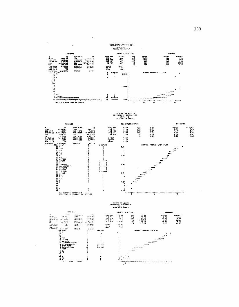
1 3 8

10TAL O rCM M M O »CVtNUt (m <VAKIAK S I A U S t lC S

YCA* • 0■c c u l a ic p s a m h c

MCAMs i o o r v m w c n u s s c v?:HtA*N-« s o n * * * « NUH •« 0

9 u * l c a pi s r JO2# 9

792 8 U .3 4 * 8 6 6 .0 2 9 .2 2 9 9 7

2 9 7 2 2 7 9 9 * 1 1 1 2 .9 * 4 9 .< 1 9 2 *

•9 8 079

0 . J0 9 > 7 8

SUN UGT9 79SUM 2 2 2 2 7 3VARIANCE 2 3 8 7 9 1 9 8M /R 104IS 2 9 .2 9 * 6CSS > 6* 4 8 9 6 1 6 95 1 0 W lA 9 * 1 .* 77 8 0 9 * ( I | 0 .0 0 0 1m t m > i s i o . o o o i

P404>Q < 0 .0 7

50 * * 1 0 2 9 1 01

o f M in

M N o r03*0>MOOC

q u a n t iL C 8 i o c r - * i

12 7 2 9)0 * *1*2691733*

123992127

52*

9 9 190S

l l

6 941 * 2 1 9 7 6 92 0 1 1 2 2 2 * 7 7 7 9 9 0 0 0 1 1 * 9 7 7 7 60 3 * * 9 9 9 4 6 6 7 7 7 7 8 4 6 9 9 9 9 9 9 0 0 0 0 1 M i l 1 2 1 1 3 3 * * * 9 9 6 7 7

MULTIPLY S 1 W .U A 7 * 9 1 0 * * » 0 J

127296 9 8 9*7* 1

99252*33*

lO V tJT13*39 2*3932*52*

HtcHcsr6 9 2 96 9 6 971* 6

29 9 3 632 1 2 9

RETURN ON ASSE r s U N IV A R IA IE S 7 A M S 7 I C S

V IA * « 0 REGULATED SAMPLE

Q U A N 1 I L C S { 0 r r s i | )

MEANs i o O tVs k e w n e s su s sc vI r n r a n «oSUN RANKNUM - a o DlNUITMAL

796 . 6 9 1 2 9 I . f» 109*1 0.0t*?9I? 1 A M .93 > 5 . 1 0 1 6 5 6 . 4 * 7 * I960

790 . 0 6 4 M J

S U M L I A /8 6 *6 6 16 7 8 * 2 6 0 ? >l>8(3 76 76 *7 6 0«i 7* 0 2 7 2 1 6 72 6 7 3 7 8 70 26 6 2 6 9 1 5 6 9 6 6 0 0 1 * 6 / 9 2 * / 61* 0278915 4 2 2 6 / 1 5 6 6 0 1 1 / 9 0 2 )5 4 / 7 1 5 5 5 6 2 5 1 5 * 0 / 1 5 2 2j 5 0 6 *4 6* 6'I*

s u m w c ? sSUMVARIANCE M ill I O S I Sr s sS IO M r ATI f*06>iii p r o n > i s i

P ft00> O

7 95 2 4 . 7 7

1 . 0 2 2 0 . 2 1 1 6 9 2

7 9 .7 1 6 1 O . 1 1 3 7 * 0.0001 0.0001

> 0 . 15

i n n f m ax 7 5 1 Q1 5 0 * MtO 2 5 1 Q1

OX HIM

HANCfq ) - Q iM o o r

6 . 8 * 7 . 38 6 . 6 1 6 . 0 /

* . 9 11 .3 15 . 6 7

6 . 9 *I1II

5 . 9 *I1II

* . 9 *IIII

9 7 *95%9 fH10%

5%1%

8 . 8 * 8 . 6 J 6 . 2 * 5 . * 7 5 . 0 6 3 . 9 )

t o w r s f 3 . 9 3 * . 19 * . 9 6 5 . 0 6 5 . 2 2

n t o n r s r 8 . 5 6 6 .A J 8.66 4 . 6 7 6 . 4 *

n o r m a l p r o b a b i l i t y p l o t

M ULTIPLY S U M . LEAP BY I O « » - f l l

Af 1 URN r*H 10>U IY I»VANtA11 31* 1181ICS

V»AA - 0 M rouL A irn SA M rir

ORA*III 1Sf 077"* I

MCA*s i r o r v S K lw af5Su n s

SfiH AAMR HUM •< 0 R.NORMAL

SUM VRIS SUMVARIANCEHUNIOSISCSSSIR MCA*

* H I8 »R fl> IS |

• 0 . *A II 4 . 112!

• n . « /49A*M /86.2 60, .-7J*I * . 7587

•509 79

0 . 111341 r * 0»:S lfM L(A7 76 8 2* 3 72 I r o18 360•6 a . v o r ri* r * 4 6 i* 9• ? im*336/7T?j6? 10 0 •9646/ 84? J* 76 .■’ '•34/0039 6 ?H6A4f i J J6AA7* * 447 2 70 4 ?•0 -2 • * *•6 4*•6 6

79874.01 39. 8*26

2 . 3JA02 J 1 0 /.It

0 . M O I/.6 0.1X101 0 ,0 0 0 1

0.016

50% * 1 0 23% 01

n f h i *

■ AMfil q j .Q i M1>0»

2 / 43 13.48 tn . a

99%33%90%

2 7 .6 5 •4 *9 I / . 77

i J6999 - * . * )

i n v r s l *9 41 * / , 77 •7 J4 - * .* J <1. AI

I l i n r i S f 18.6

• 4 . 79 22.27 2* J J 21.85

NORMAL f*OOA811I IV

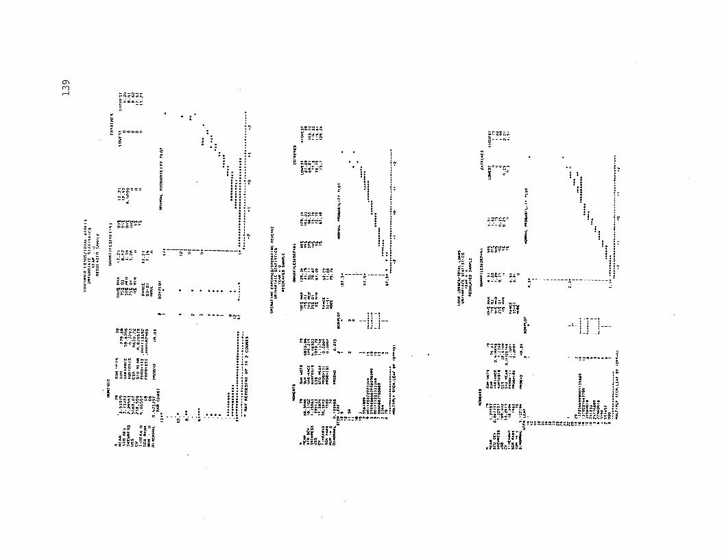
139

r-

• “ cft, -

§ y i

riis i *S£2S =?ss;- = SI :s sM Isisi - 5SSgss 1̂ 1 |-

:: K •: : I.

j - r • * • «

;i j i ?NilMi.ii'

Ss«« § i*'5

; sss=s-'

S t : S S S S 5S:cJ5*SJ g .

fsss* hi

I

1 1 1 t

i l l i£££jSS?SSSg

=3>s =e

Ji:

. • . v . . ' : s » »

5?P.ll

111

|J

Es-S;!|| g

! ! IS f

TA M

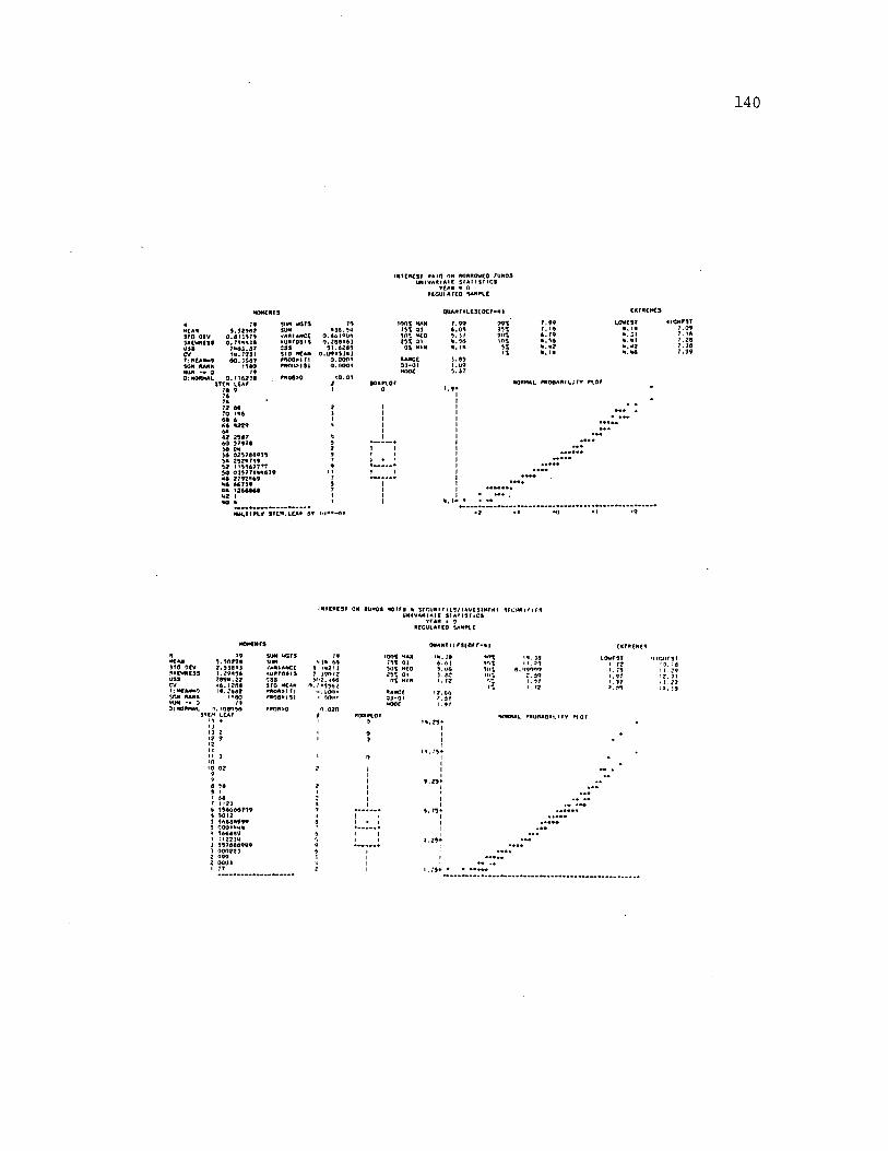
1 4 0

m rcR C S T » ju n o n *0 * 110*20 ruHOSUNIVARIAIC S fA M S T IC S

r tA N • 0 RCGUIATCD SAN*L£

<JUANHLC3(OC7**l

NCAAsro oev SitW N C MUHSCV7 ; mCAN«0 s e n IUNN NUN *• 0 0 : NORMAL

o . a i m s0 .7 9 * * 1 9

2 * 6 3 .3 7 l u . 7 2 3 l 6 0 . 16 4 ?

*5*0 »9

0 .* 1 6 2 3 0 S T tN LtAC

70 9

JIM WCTSSUNVANIANCCMunrosiscssSIO NCANm o o » t r i **r)i*»IS»

r*o9>0

79N S6.SU

0 .6 6 l « « *0 .2 9 0 * 6 ]

5 1 6 2 9 50 .0 9 1 6 3 * 1

0.00010 .0 0 0 *

<0.01

loot HAN 75t 03 )0t Hto 26t Ot 01 MINJUMGC0 1 -0 1hooc

7 .9 9 6 .0 6 6 .1 7 U .9A « . 1«

9 9 t9 5 t 91 i t 6 . 79

*.66 * .* ?

NORMAL A RO 0A niLi7Y AL07

MICMMT7 .0 9 7 . 16 7 .2 97 .1 0 7 .9 9

72 96 70 196 66 6 66 9 229 6492 2 607 6 0 97970 SO ON) 6 0 2 5 7 9 9 9 1 6 9* 2 5 2 * 7 6 9 52 1 1 5967777 50 0 3 5 7 7 9 * * 6 7 9 • 0 2 7 9 2 6 6 9 6 6 6 6 7 3 9 *• *260040U2 I NO «

M K .n n V STCH.LCA* 0Y I ..

I N fC * (3 7 ON 80N 0S * 0 7 7 9 * SrCUA I 7 11 5 / I NV( JIM f HI i f r .U N in C S UNIVAN I AI f SlAIISriCS

i r k n • o * c c u l a ic o SA M nc

•HANs*o ocv1KWNC3SUSS

795 .5 0 2 2 9 2 .9 1 0 * 3 1 .2 9 6 9 6 2 9 9 * .2 2 * 6 . 12(10 1 9 .2 6 4 2 1 6*0

79

s u n w orsSUMVAN IANCt «U N I09 I9 CSSs r o mcan•NON*I 7 I '" Q 0 » < S I

79'• 1 4 .6 6

6 '* 2 11 2.1907? 5<i?. *66

o . .* •9562(I.UOM • 00* *»

loot RAN791 01 s o t MCO29* Q *ot M*NNANCt01-01HOOC

9 U A N i i t r s ( o r r - u i

I * . 10 t o t

1? . >1 U.22 i * . J9

NORMAL ANOflAOM.irY *107

a *69 17 64 7 I 121 6 9 9 6 6 6 6 7 0 9 6 00*2 5 5 6 4 9 * 9 9 9 9 OOOIUUN * 5 6 64*9 '» 1*2214 1 5 6 7 * 4 0 9 9 91 0002232 *99 2 0001 I 77

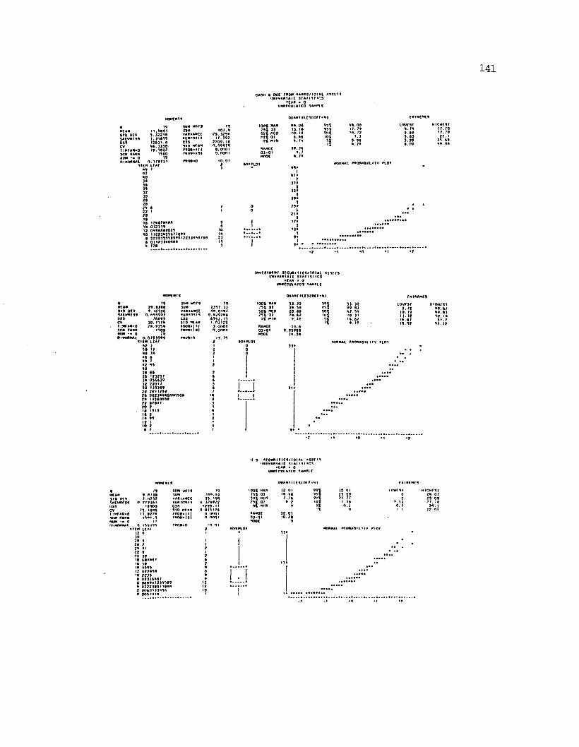
1 4 1

CASH * OUf ' * 0 * N A N IS/IO IA C ASSCI9 U M IVANIAIt STA 11 S I ICS

YtAN « 0 U H iiro u tA iY o s a n h c

Q U A N T IU S fO C 7>* |

Mf AMs i o oev9 « c w n r s su s s

T9I I . *861 9 .3 2 2 '6 3 .3 * 6 9 1 1 7 6 ) 1 .8 * 6 .3 3 9 8 1 9 .1 8 7 2

1980 T9

sim w n isSUHVARIANCE■UNIOSISCSSSIO Mf AM P N O O H It m an* 1st

n »o«> o

T9 9 0 7 .4

7 6 .3 2 9 * I T . 591

7 7 0 9 . J 8 4 ,9 9 8 7 9

9 .0 0 0 1 a . o o o i

<0.01

I o a f HAM 781 0) 5 0 1 MtO 791 01

a t h im

■ • .0 6I ) . 16 •0 . 16 9 .4 6

19 . ) • 4 . 7

■ . 7*

9 9 19 9 194*

■■. 09 17 . T9 >6. T?

u o w rs i4 . 74 8 .6 9 9 .8 3 9 .9 8 6 .0 9

H ic H c s rIT . 76 1 7 , T9

7 7 . I 2 9 .6 9 M .0 6

NOOMAt. rH O flA SItlT Y H O I

IJT »

I

1616 1 7 * 6 7 6 6 6 6 9 |1* 0 1 7 ) 1 9 6 112 0 * 9 6 8 8 9 0 2 9 10 * • • • «10 1 1 2 2 3 4 9 9 6 7 7 6 9 1 I*

6 2 7 2 2 3 9 9 9 6 9 9 9 1 7 7 )3 * 9 6 7 6 8 7 )6 0 1 1 2 ) 3N6666 11 1* 776 3 1

7 9 *I

7 9 *i71 •I

17*I

I I *I

9*I

MY AHSIO OCV SJUMNYSS USScvI M H f O s o n AAMI HUM '« 0OiHOHMAi

797 9 .6 1 9 69 . 16996

4 .* 9 9 9 9 7 T6899

) 0 .T I7 H 7 6 .9 ) 9 6

• 9 8 0 79

0 .4 7 9 ) 0 9 6 SI CM U A f

92 )

SIM WR1S SIMVAAIAMCC RUHfOSI*CSSSTD MfAMr n o O H H■NON* I SI

T92 3 9 7 . ) ) AH.0 1 6 7

0 .■ 7 9 7 * 6 6 9 9 3 .1 9 1 .0 ) 1 2 9

0 .0 0 0 1 4 .0 0 0 1

• 4 . 19

• 2 *9 *036 6636 1 7 )2 9 7)■ 0 9 6 6 3 932 77 0 1 730 1 )9 3 6 97 6 7 9 * 7 7 9 97 6 0 Q 2 )* 4 * 6 8 4 fl1 6 62* II9 6 0 O 9 672 6 7 6 1 77 0 716 I 9 U16 2IH 9912 I10 2

IMVCSIMCNt SC C U R IIIY S/T O IA C AS9Y7S (M IVAHtAIC ST A M SM O S

r€AH » O IMHCCUIA1CO SAMHC

I I

ouAMi i i c s m r > * i

•O O f MAM 7 9 1 0 ) 9 0 1 MCD 7 9 1 01

4 1 HIM

NANCY03 * 0 1HOOC

93 32 3 9 .9 8 78 86? * . 62

9 . 77

* 3 .69 .9 9 9 9 9

3 6 .9 6

9 9 f9 9 19 4 f

3 3 ) 2 ■9 93* 7 . 9*1

L o v r s r 9 . 72

10 . 19 13. 17 • * .6 7 1 9 9 7

M fRtirST * 9 .6 7 * 9 .8 ) 9 0 . I*

9 » .7 9 ) . 32

•OHMAI. M 4 R A 8 IIIT V H O I

4 S . SYCVHI f I C S / 101*1 ASSYIS 1MIVAH1AIC | l » l 1 1 1 ICS

»tAH • 0 U M M ffflHAirn S AMH f

NY ANSID OCV i K M i r s su s scvI ? Mf AHaQ SCH • • • ■ HUM • • 0

799 N 7 36 7 .(1737

4 .9 7 9 1 6 1 • 7 4 0 0

79 . 1SU8 • 1 . 8 7 7*

1 9 4 1 .9 17

4 19*119*9K M CCA7

32 4 1078 3 76 7 7* I I 72 9 70 39 18 6 6 1 * 6 7 16 96 16 9 9*9 12 0 7 7 * 9 6 •0 7 7 3 9 8 0 2 ) 3 6 * 6 76 8 8 6 9 0 1 2 3 9 9 8 9 * 0 7 7 2 3 6 0 1 1 6 6 87 0 0 6 0 1 I3*9A 4 0 0 9 7 1 1 *

SIM w n is SUMVANIANCC ■UN70S* * CSSS t o MIANr * 0 8 > | i |■ N o n v is l

•**4N»4

8 4 .0 3 9 . *4* 7*V 77 9 6 . I t 19176 .0 0 0 1 .0 4 0 1

'401 «*" 791 03) l» l MCO

Na n c C03*01MOOC

Q V A N » u f s in r r - « ‘»i

I? 01 9 9 1I * . *8 9 9 1

7. 76 7 l i f* 7 »01

37 01 79 09 71 27

MCHfST 2* 07 29 09

NONNA l »flOftAAI1.1 1V f ) 0 »

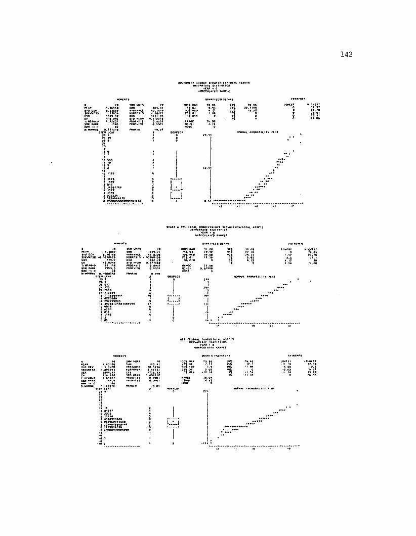
1 4 2

OOVfNMtM? AOfMCY 9CCUMI M C 3 /1 0 IA I A S S ftS UMIVANIAft S IA M S /IC S

/CAN • 0 u tm rc v u T c o vw « n e

Q tlA N /U C S f 0 t r > 4 |

4 79 SIM WOTS T9 100 1 MAX 24 06 9 9 1 2 4 .0 6Mf AM 3 .4 6 6 6 4 SUM 4 6 3 .1 1 7 9 1 Q1 4 41 9 9 1 2 2 .1 / 9 99 / 0 OCV 6 .3 3 6 3 9 VAN1AMCC 4 0 .1 9 1 9 9 0 1 MCD 6 2 / 9 0 1 1 9 .5 234CWMCSS 1 .3 3 0 9 4 RUN1QSIS t . 161 /1 2 9 1 01 1 • IN 101 0OSS 9 0 4 9 .0 2 CSS ) 1 ) 1 .0 9 0 1 HIM 0 91 0c v 1 0 4 .0 4 6 9 1 0 Mf AM 0 . / 129 1 a 1? Of • MfAMaO 4 .7 2 6 3 1 7N04> f l 0 .0 0 0 1 HANOC 24 06SOI NAHN 1040 t n o o m s J 0 .0 0 0 1 QS-Q I / 39MW 0 66 14J0C 00 : MOMMAL 0 . 1 7 7 )4 9 7NON>0 « 0 .0 f

9/CM ICA f r 404 7 1 0 /24 1 1 0 2 4 .9 *21 19 2 02 2 8 1 0

MIOHCSTi r . 9 /zz. /a 210/ 2 ) . 91 2 4 ,0 4

t« 01 / T14H > 99 in / a15 9 I ? a f tio u nf• itn/ 1349 4 o nJ J 4 9 6 / / N ?6 33/9 I J J 8 9 ? UOI234 I 0 2 3 4 4 4 6 / /4 0 0 0 0 0 0 0 0 0 0 0 0 0 0 0 0 3 4 /4

i« * r < • t o i l n e a t s u o o iv i s < o * 9 u c w i T i u / t o m A s s r / sUMIVANIAIt } U l t ] I I C )

VIA* » o U N N fG utA tro A A M nr

0UANIHCSI0C/-4

••t am n . i a a /91 0 OtV 4 . 4 6 / 4 4s t f V N r s a - o , o i / 0 f i ? 4USS CVi • mvam*oSRM NANN MUM ’ « OOfNOftKAt 0 .0 9 0 4 3 6 4

5 l f H I f A f

7 1 9 / 6 2 .0 2 0 9

2 1 .1 4 0i3 » m .9

91 Mt w n /3SUMVANIAMCC■U N f/ISIS * C399 1 0 MfAM 7NOO>I 11 f n o o > |0 |

7N«N*0

30 I 24 0 26 OIT 29 129 22 2464 2 0 1 • J 3*3 >0 1 1 4 9 9 4 9 0 0 /Ift 0 2 2 ) 6 4 0 19 2 4 / /9 9 0 1 9 12 J 4 ZO01 2 4 9 6 /0 6 4 9 9 9 10 4 0 1 4 4 6 6 9 04 o n4 1141 2 1 0 09

791 2 1 9 . n 4 1 .4 ) 0 6

.0 0 1 6 9 1 1 6 J 2 4 2 . / 9

0 . > 2 /6 4 0 0 .0 0 0 1 0 .0 0 0 1

0. 104

Z 9I ( 5 0 1 >2 3 1 <

31 04 2 / . 14 7 4 . 1 1 5.92 6 . 12

NOMMAf. 7NAMAMH.11V *101

UlCWfST 24 092 / . 14

7 t . I

0 t f r t o tH A t r u * n $ / i o i A i a i a / i l/MIVANt A l t S IA IIS M C S

YfAB » 0 UNHrCU IA lfO 3AMVIC

O V A N tU M IO tf«<

MtAM 9 1 0 OtV 3 > ( M / » VS*

6 .6 0 0 1 4j . )'«?a

0 .0 6 3 9 4 )3 0 9 4 .4 /

t 0 1 4 )9 /1 l l t M LCAf

26 *

JIM v f t /4SUMVANI AMCC ■UNfONIN CSS9 1 0 MtAM M 0 « » I 11 TNONAlSj

ANON»0

7 2 2 6 .9 9 0 6 0 1 1 1 2 0 0 001 0 .0 0 0 1

'0 0 1 mam >91 0 ) 5 0 1 Mf 073 1 01

O f HIM

4AMCC0 3 -0 1M W

9 9 f9 H9 0 1'0 151

lO W I I • 1 1 10

• 6 .0 4 •2-09

NMMAI AN OMAN I L I / V '

14 3412 0122/*0 2 9 0 )a i i n a6 0 0 4 4 9 0 0 6 4 6 6 0 ) 3 9 6 0 1 9 9 6 4 4 2 2 3 4 M 6 /4 4 9 0 I4 9 0 9 / 1 9 0 1 6 /9 0 •0 40000000000OOO•2 r-4 • 6 0 •4-10 7

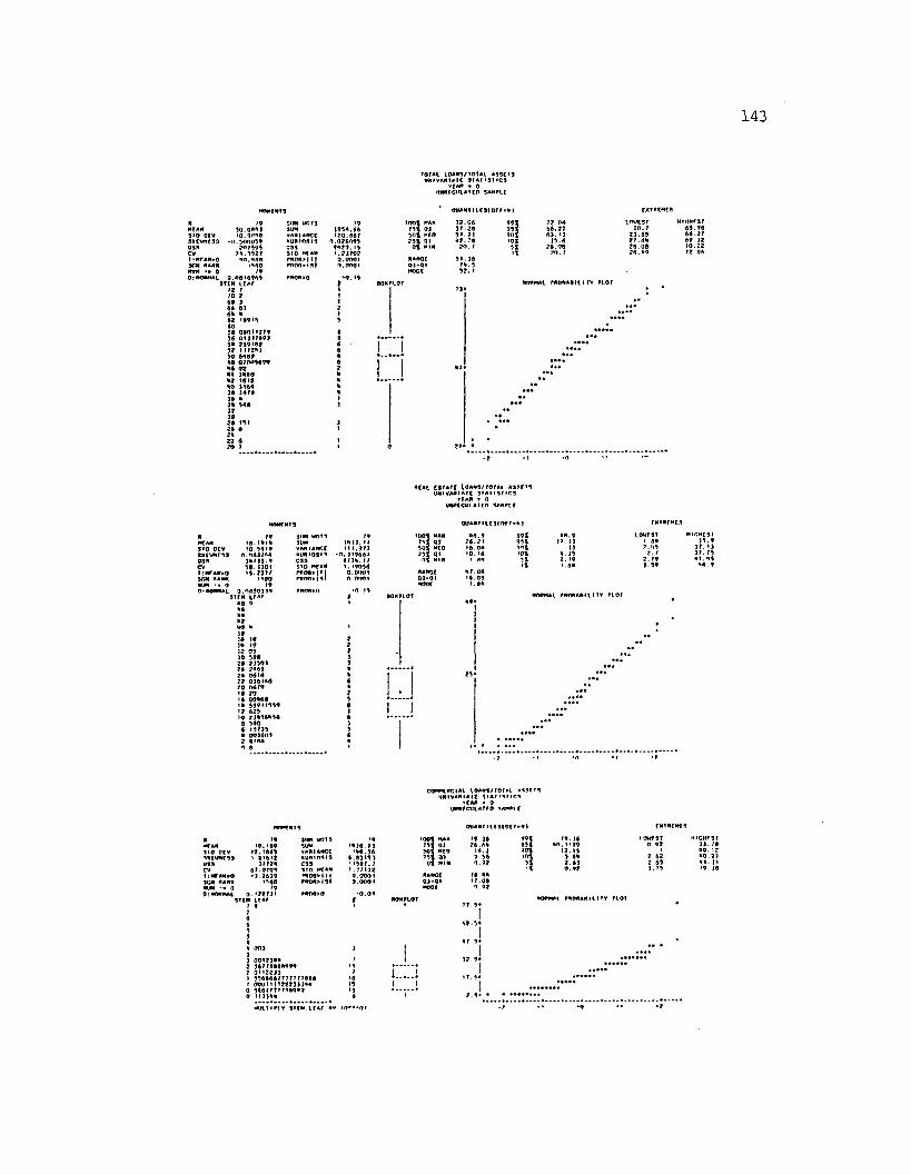
1 4 3

TOTAL LOANS/TOTAL * 1 3 0 3 UNIVAN t AIC STA TISTICS

y c a n • o im ru G t’t A i c o SA M ftc

nc an SIO OtV 3RCWN(33 OSS CVt;H fA N » 0 SON NANNm rn • • oOTNONHAl

10.0A1) •0.9 009

-■1.50TI059 2 0 /9 9 4

2 1 .9 9 2 7 i n . man

■ 540 It

0 .0 9 1 4 9 4 9 S K H (.(A f 12 t TO 7 69 1 6 6 0)66 662 X 9 1 4 60$6 090H279 16 O U T /6 9 1 96 2 0 9 1 0 9 92 t• *****90 6 6 6 9 66 0 /0 0 1 6 9 9 66 0 2 66 166 0 62 1912 6 0 >166 >6 1 9 /6 16 6 16 1 6 9 12 10

SIN* WOTS SOMVANIANCt■UNIOSI3CSSS ID Mf ANmos * tt Nnofl>ist

It1 9 9 6 .6 4 < 7 0 .6 9 /

0 .0 2 6 0 9 9 9 1 2 9 . i s 1 .2 1 /0 2 0.0001 0.0001

>0 . 19

t o n s ►75X CSOX Mtl) 251 Ot

O t MIN

SANQC01-01MO0C

0 U A N M L C S (0 (/> 6 |

7 2 .0 6 9 9 19 / . 2 9 9 9 19 1 9 1 9 0 16 2 .7 4 101

2 0 . / S IJ 9 .6

2 9 .0 9 2 0 . /

io w c s t 2 0 . 7

2 1 .6 9 2 / 6 6 2 9 .0 62 9 .6 9

HICMtST 69 . 99 6 6 .2 7 69 12

NfAN3 1 0 OtV SNCVNfSS OSS cvT*NTAN«0 STM NANN NUN - • 0*••0*6*1

>91 9 .1 6 1 6 1 0 .1 4 1 9

0 .0 4 1 7 4 6 1 6 /1 1 .9 9 9 .1 1 0 1 1 9 .2 1 7 /

1390 19

0 .0 4 9 0 1 1 6S ftM t f AT

64 96666*760 61916 1916 <912 0510 90429 2150120 7<i4l26 06< 622 0 1 6 IA 620 0 6 /910 20<6 00 * 6 416 5 9 9 1 1 9 1 912 629>0 7 X 9 6 6 9 40 5 9 06 <97)5* 0 0 ) 6 0 )2 « INN0 0

s in v o i sSOMVANIANCt MON 10313c s sSIO MfAN m o o * 1 1 1 n to n * I S i

M 0A >0

NCAL ESIA1C lO A N S/IO IA L A S S fU UNIVAN I A l t STA TISTICS

YfAN * 0u M N tc u iA itn SA N Pir

Q U A N M lC 3 (0 fr« * >

791 411 . 1 / < 1 1 .9 /7

• 0 .1 1 9 6 6 7 9 1 1 6 . 1 / 1 .< 9 0 9 6 9.0IH M 0 OO01

»fl. 19

1001 HAM 791 01 9 0 1 NC 0 2 9 1 01

o t NIN

6 6 .9 2 6 .2 1 1 6 .0 6 <0. <6

6 / . 06 < 6 .0 9 1.66

99 1 9 5 1 9 « 1 ■ 01

HI0HCST 1 1 .9

17 . 11 17 . 75

NONMAL ANOHAftltlTV 7101

CO***C*CIAl LOANS/101 *1. * 3 3 / 19 UN I VAN IA11 S 1A M 3M C 3

YfAN • 0 U N NfCO lA irO 3AMKC

■ t AN110 OCV SUfVNfSS USS

It■ 9.< 49

12 . 1469 i 4 1 6 1 2

1 7 /2 6 6 7 0 1 0 9 <) 761 9

• 9 6 0 19

SIM W013SUMVANIANCt■0*10919CSSSTO MfAN 2 6 0 9 * ♦ 11 MNON>IS f

*NfM>0

19• 4 J 6 . 9 I

1 * 9 .5 6 6 .9 ) 1 9 1 1 1 1 9 7 .7 i . 1 /1 1 2 0 .0 0 0 1 0 .0 0 0 1

'0 . 0 1

■001 NAN 111 01 501 Mfo ? 9 i a s

0 1 MIN

■AMCC0 1 -0 1NOOC

Q V * N M l(9 IO C r> * |

7 9 .1 6 9917 6 .6 6 991

IA . J 701

79 66• 7 .0 9 0 . 97

1 9 .1 6 6 0 .1 • 9 9

12.19 5 86 2 .6 5 0 .9 7

2 .6 2 2 491. 71

7 7 .9 *NONMAi M60NANILUV *LOI

• 0 . 12 6 0 .2 7 « ) . I I

6 00) 1] 0 0 1 2 1 6 6 2 96 7 7 0 4 0 6 9 9 9 7 01122111 9 9 6 6 6 6 /7 7 7 7 7 7 0 0 4 t 000111127211)66 0 9647TTTIM N499 O i t ) ) * *

4 2 .5 *I6 7 .9 *I1 7 .5 *I< 7 .9 *I

2 .9 * '

MU11IMY STfM I f AT NY

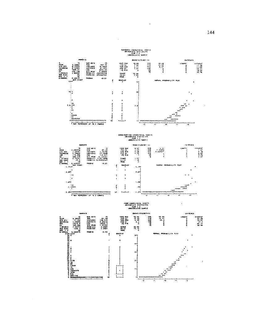
1 4 4

com sum c* l o a n s / 10141. * s s r nUNIVAN IA I f S f AI IST IT S

’ CAR « l» UMKCULAIIO iANRI.f

OUANI l l . f S( Of, I ' *1

(•CANs r o o c v sscw N C sa u s sc vT:N<AN»0 9CN AMR MUM *« f» 0 : NORMAL

toj . f s a s i 4 .7 9 0 7 5 7 .7 2 9 * 9 7Q 9* .71 2 3 2 .> 4 9 I . 5 2 0 0 2

64 64

SUM VC3SSUMv a r ia n c ea u r / o s i sc s sSrO NfAN M o a » i r i R * 0 8 » IS I

RR06>0

792 ? r . ; ?

7 6 .9 4 6 9 4 . 1499

9 9 1 2 .2 2 a .9 6 * * 0

0Q O 2993'i6 0 « J« 4 7 * 0 3

<0 . 0 1

IOO* MAXr s s o i9 0 1 MCO 7 9 1 01

•)* M l*

AANGC01-0** o o c

1 1 .5 2 I * . 11 '5 . 5 2 1 6 .0 0

NORMAL R R O (U « iL irv RLOT

• MAY RCRHCSCNf UR fO 2 COUNtS

CONSTRUCTION LOANS/lOlAL *551 1 4 URIV ARIA If 4 IA IIS M C S

’ Car » <»JM C O ItlA IC ll 4AMV1 c

o m a r t h t s i o r r 1

NfANs i u o c v 4NIWNCSS

SON RAMINUN ~ i i* OlNOOMAL

U .2 9 6 0 7 4 I . ?0*I41 5 . 0 K 2 2 119.194

SAN CHART

SUM WQISsum/AOiAwrc AURfOSiS CSSS IS NfANp M 0 R * tn O .o j A *06> I1 I 0 .0 0 9

71.19 .'■ *19* 7,7906 12. '«7l 11 5 1 0 1 l i J 9 A 8

5 1 4 9

1001 NAN 751 OJ 9 0 1 HfO7 5 1 01

■ANCCO J - HNOOf

•M1RNAI R *08A 6IL lT V ALOf

0• MAY ACRRCSC87 UR 70 7 COURTS

TARN LOANS/1 0 1 *L ASSCTS UNtVARIAIC ST A T IS riC S

’ CAR • 0 VRRfCULATfO SAMRLC

MCANs r o o c v

u s s

799 . J 0 9 9 9

H . J 9 * 1 .5 5 4 9 5 1 1 0 1 * .9 1 2 0 .9 6 9 7 .1 * 7 5 1

1 1 0 9 .5 64

SIM UOTS SIMVARIARCCr u r t o s isc s sSIO M f** M o « > m R * 0 6 > ls l

R *oe»o

797 * 1 .* 9

1 2 6 .9 1 * 2 .2 9 1 i f 1 0 0 9 9 . 3 1 .7 1 7 * 1

0 .0 0 0 1 0 .0 0 0 1

< o .o t

l o o t MAM75? 03 5 0 * MCO 79* 01

0 * MIR

•ARCf0 3 -0 1NOOC

O U AR fILC9|0C C’ * I

5 0 .* * ' 9 9 *15 *5 9 5 ?* .9 9 90*

9 Q .* « 1 4 .9 1 2 5 . 1

KtCMf ST 1 3 .2 9 > 4 .9 1

1 7 .1 * « . 77 9 0 • •

NORMAL 2*0 6 * 6 1 LI TV ’ LOT

I 609I 1*691999 k 1250 I *70 • 0*971*9I 00000000000000111133**9902J966 «0

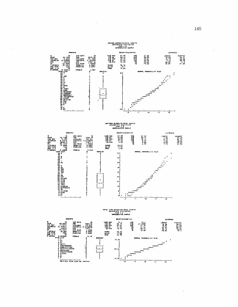
1 4 5

m h a m o o c p o s i t a / i o f A i a s s f t s UNIVANIAIC S 7 A II9 H C 3

u a n « o UNNfGUlAICO SAMftC

NfANSIO o c v SRCwwrsa u s s c vT:MfAN»o s o n NANNm m *■ o

79I S . *222

9 .6 9 2 4 0 .5 4 4 6 8 1

113*1192 7 . 4 4 2 *1 2 .3 * 1 5

n e o19

. 1009*2 s i c h c tA r

40 0 9994 109 94 9 99 9 90 •4« o r 44 4 44 0996 42 440 I99«»J9 6889 14 049901*9 14 J940499 12 44494947 10 12918890)1 24 21419 24 0078*19 24 990 22 014 20 9 14

s«m w i t sSUMVANIANCC HUB1 0 9 «9CSSSIO NfANr * 0 8 » m7NOH>ISt

M O 9>0

192 7 7 4 .4 9 9 ) .1 6 8 8

0 . 3 5 407* 7 7 4 7 .1 4 1 .0 8 9 9 8 0 .0 0 0 * 0 .0 0 0 *

.0 4 7

100 1 MAA 791 g j 90S NCO 2 5 1 01

0 * MIN

NanCCQ l-Q IHOOC

o u A H f i t c s t o c r - B t

4 1 .0 9 9 9 14 0 .1 2 9911 3 .7 2 90S7 9 .4 2 1011 4 .8 3 91

4 4 .* '2 1 0 ,7

• 4 .6 1

6 1 .0 9 9 6 .0 6 4 9 .6 7 2 4 .9 3 2 0 .9 9 ■ 4 . 6 )

L0VCSI1 4 .6 )1 9 .7 4

1 7 .62 0 .9 92 2 .0 4

MICIIf 57 9 4 . 9* 9 6 .0 6 9 6 .9 6

9 » .2 6 1 .0 9

NOBMAt 7B 0 0 A B H .il '

s a v in g s o f r o s i i s / i o i a i A s s r t sUNI VAN IA I f S tA I M I I C S

rfA N • 0 UN NfCULAirn SAMNIC

* 79 sim w o ts 79 1001 MAX 57 99NfAN 7 2 .1 ) 6 6 SUM 1 7 4 8 .7 9 791 0 ) 1 0 .0 6SIO OCV 1 2 .1 3 7 VANIANCC 1 9 2 .2 0 1 5 0 1 NCO 1 9 -9 5S«(WNCS9 0 . 79924 ■UNIOSIS 0 .0 * 2 9 8 7 9 2 9 1 0* 1 2 .5 2USS 9 0 9 8 1 .9 CSS 1 1 9 7 1 .7 0 1 MIN 92CV 5 5 .7 3 1 2 SIO NfAN * .> 6 8 0 2);M fA N *0 •9 .9 4 6 3 f * 0 8 » m Q.OOOI BANOC 51 67se n BANK I9 6 0 **rm » I s 1 0 . BOO* 0 3 -0 * 1 7 .5 4mm *<• o 19 HOOC 1 9 2OfNOMNAt 0 .1 0 9 9 9 **o n »o 0 .0 * 4

S U N L lA f i s o x f t o r9 6 6 3 5 1 *54 I92 6 i 150 6 t 11*49 |46 7 * 14 * 04 2 45*42 14 0 4 1 119 02 2 19*16 066 1 134 504 1 112 569 3 11*10 I* 2 J29 99 2 126 297 3 77*2 4 6 9 * 9 6 4 4 I2 2 9714 12 0 4 174 4 21*14 1899 * |*4 1449 4 | I I14 2 3 1 4 9 3 6 7 1 • 9*12 0 2 ) 8 6 8 6 7 9 9 I*0 19 2 1

6 1 112448 7 9*4 9 7 8 9 4 !4 4* 2 19 9 I j* •

Q llA N II lC S (0 f7 < 4 »

9 9 19 9 1901

1118 . 17

6 .2 9 4 .4 6 1 .9 2

MCM75I 45 19 4 6 . 71 9 0 .9 8 52 9 15 7 .5 9

■ONHAL NNONABILIt

i o i a i r i » c o f r o s i r s / i o t A i i n n i UN I VAN I Af | SIA M S M G S

T t AN • 0 IfNRCCUiMCO SAMNVC

NfANn o o c v» ( W * ( S SV9SCVIfM f AMaO SCJI NANN MM • • 0 0 ‘ NONMAl

794 4 .6 5 2 7 * 1 .9 * 1 7

- O . *94951 14 )0 * 2

2 9 .5 1 7 1 1 4 .6 0 9

1980 »9

SUM WOTS 79s*m 1 6 6 9 .9 4VANIANCC 1 4 1 .9 ) 7AUNI<3<1I<I • 0 .0 ) 1 4 1 6 *CSS SIO MfANn*o o > | i i►NOB*151

0 .0 6 5 * 4 4 7 * 0S U N I tA f

7 97 0*6 978 0011*9 9 9 6 7 7 8 6 6 6 9 9 9 0 0 0 0 * 1 * 1 )3 4 4 4 9 6 7 7 7 7 7 7 7 6 6 8 9 9 4 0 0 * 2 2 3 1 4 *1 5 9 * 7 7 7 7 7 8 9 9 4 ) 11232)2 57 2 01

110 7 * .I .3 4 0 4 0 .0 0 0 1

1001 NAN791 0 ) 50 1 N<0”4 2!.NANGCOJ-Q*hooc

o U A N H L fS iO fr .4 1

7 9 . ) 9 5 . 19 47 21 1 7 .5 1 14. 98

9 8 . 72 1 7 .4 4 1 6 .9 6

9919 5 19 0 1

’175 . J

6 7 .0 7 9 96 1 . 1411 5»2 9 . 15 1 6 .9 4

(.OWMf 16 58 1 4 .9 ) 20 . 61 25 . *5 2 4 .6 2

NONNA L A* ON AO H . I IV H O *

Nicutsr 6 4 . 9* 6 7 .0 6 6 4 . 5 '7 0 .6 *79 )

•N N IIN tV S U N . I f A f 8V IO **«O t

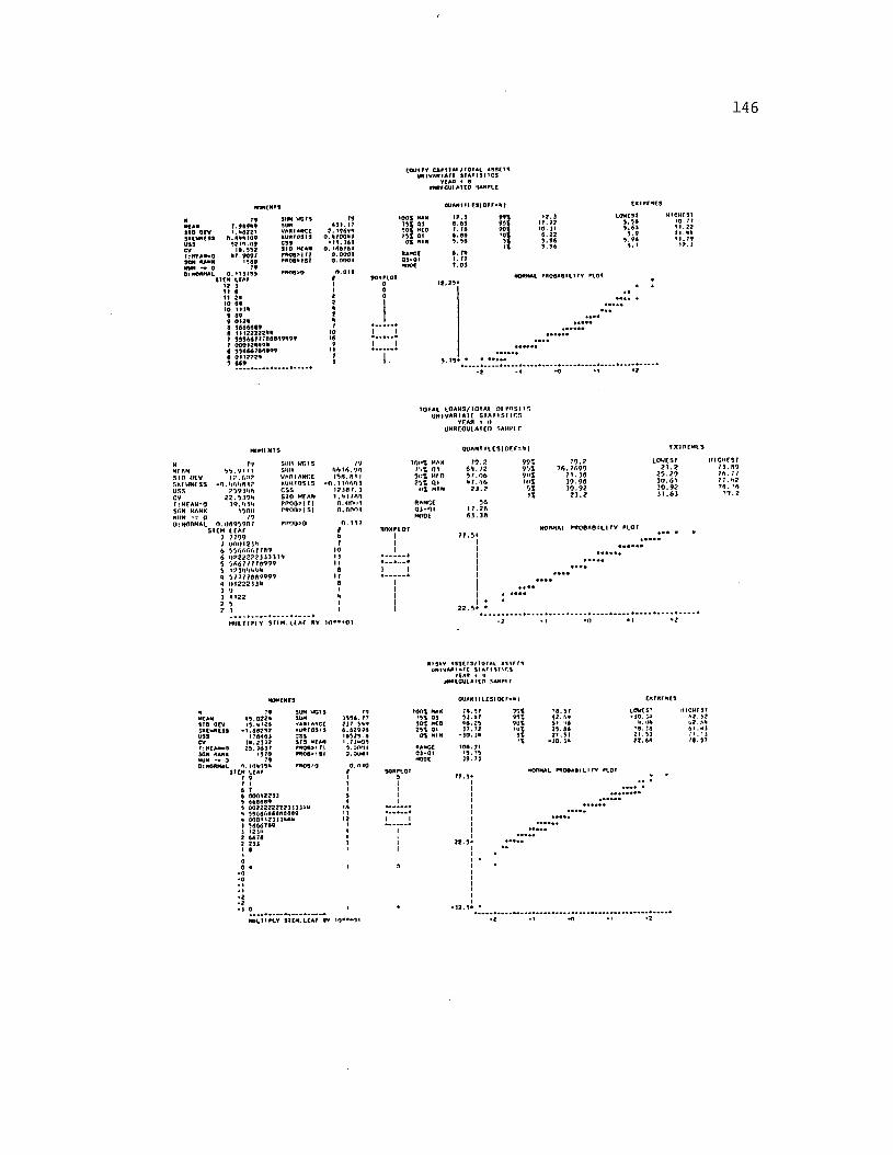
1 4 6

COUIIY C A M 1 A I/I0 1 A L A 9SC I9 UNIVANlAfC S IA M S H C S

ycao » 0VMM GUI AT tO HAMPIC

NfAH9 1 0 OCV SRCWNfSS 1733 CVItHTAINO SOM M M HIM • • 0 OtNORMAL

7 f7 . 9 9 9 * 91 .1 9 2 2 1

0 .8 * * I O ? 5 7 1 1 .0 *

i a .5 5 2 * 7 .? 0 9 7

i9 6 0 79

SIM V CfS SUMVANIANCC■imiosisc s sSIO MIAN « O f l * l 11 N * 0 6 » IS i

M fl8 > 00 . 1 1 )7 8 5 SU M LCAf

I ? 3 I I 4 I I 2* t o 69 •O 1131 * 8*9 0 1 2 9 • 1 6 6 6 6 8 9 8 11122222**I 5 9 9 6 4 7 71 8 8 8 8 9 9 9 9 t 00012****4 3 9 6 6 4 /6 0 * 9 94 011722*5 4 4 9

796 ) 1 . 17

2 . 196V* 0 .1 1 0 0 * 7

17 1 .3 6 1 0 . 166761

0 .0 0 0 1 0 .0 0 0 1

0 .0 1 2

hanccQ j-Q INOT*

a u A N M te s < o c r« * t

6 .7 * 1. 77 7 . 0 )

1 2.) 1 1 .2 2 10 . I I 6.22 9 .9 6 9 .5 6

lowcsf 9 .3 8 5 .6 3

9 .9 3 .9 6 6. I

HI GHC3I10. 17 1 1 .2 21 1 .* * 1 1 .7 9

17. I

NORMAL FR 06A 9IL11V U O T

101 A t tO A N S /IO IA L O I1 * n S » IS U H IV A R IA IC S (A I I S I IC S

Y fA lt » I) tlN flC C U lA IC f) SAW ’LC

Mr ANs i o o t v SM .WtU s s USS

n5 5 . 9 1 1 1

1 2 .6 1 1 ?-0.'i6»t«l?? 5 9 )* i6

2 2 .5 3 9 * 139 .* l3» i

15011n

0 : NORMAL 0 . 0 0 9 3 9 0 7

SUM WC1S n 11)0% MAX 7 0 .2SUM h i l t 6 . 9 8 »'-% 0 3 6*1. / ?VAfllANCC 1 9 8 .8 1 < 5it% w rn 5 7 . 0 6huh m s i s - 0 . 1 I ' i A N I 2 5 1 Q> * 7 . '16c s s 1 2 3 8 7 . 3 11% H IN 2 3 . 2s i o M ra n i . M / n uPflO O >l 11 o . n o n i RANCC 5 6r n o n > I s i o . o n o i 0 3 - 0 1 1 7 .2 6

MOOt 6 3 . 3 8

STCH L fA f /7 7 7 9 9 *7 000123*1 76 5 5 6 6 6 6 7 7 8 9 106 0 7 2 2 2 2 2 3 3 3 1 )»i 135 5 6 6 7 7 7 7 8 9 9 9 1 15 I7)»»*i*i*l*l 8M 5 7 7 7 7 8 8 9 9 9 9 11* 0 1 2 2 2 3 1 1 1 8) 9 13 1 1 2 2 92 5 12 3 1

M 0 L H 7 IY S M N . l l A f 8V

n o x p i o rIII

Q U A N 7 H .C S (D C f= 9 |

9 9 ? 9 3 ? 9111 10%

5% 1%

7 7 . V I I I I I I I I I \

2 2 . 5 *

7 9 . 2 7 6 . 7 6 9 9

7 1 .3 03 9 . 9 03 0 .9 2

2 3 . 2

LOWCST2 3 . 2

2 5 . 2 93 0 .6 13 0 . 9 23 1 . 6 3

incurs! 7 3 . B9 7 6 . 77 7 7 .1 2 7 0 . 76

7 9 . 2

NORMAt W O O A 0 IL I1 Y F l O l

a >s a y A s s c i 3 / i o r « i * s » r iUH»HAA»*1f S I A f lS T tr .S

> (« « • i|VMRlCULAflfl SAMR17

OVANfILCS(0€7«<

ACANs r o o e v sx c w n c ss u s s

* 9 .0 2 2 * 1 9 . (H 24

- 1 .6 8 2 9 2 1 7 0 4 4 )

1 1 .2 3 ) 2 2 9 .7 4 3 7

1970 79

SOM V CI3 SOMVAJtlANCC*0 8 7 0 3 1 3CSSSIO MfAN M o s > i n A RO 0H SI

* 8 0 8 '0L 0 .1 0 * 7 4 *3 7 CM LCA#

7 9 7 1 6 76 0 0 0 1 2 2 3 )9 4 6 8 6 8 94 002222222?))))**1 9 4 6 6 0 6 4 8 6 9 6 8 9 « 0 0 0 1 1 2 3 3 3 * * *J 5 6 6 6 7 8 9 3 I23H2 6 6 7 8 2 2331 8

793 4 1 6 .7 7 2 3 7 .5 * 9 4 .6 2 9 9 4 1 6 9 2 4 .9 ■ .1 3 * 0 5 0.001*1 Q.OOiH

0 .0 1 0

100% MAX 75% 01 50% MCD 29% 01

0% MIN

•AMCC0 3 -0 1HOOC

79%94%9U%•U l 2 9 .9 6

2 1 .5 3 - 1 0 .3 *

NORMAL R908AI

M lU 'A L V 9 7 CM.LCAf 8V IO***OI

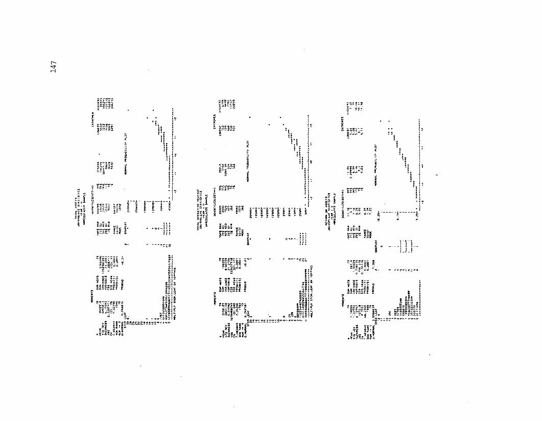
147

a

u

ft

m ’|i

ip« ij

j HP ip n r mhhl u. 5

hi r

H I lr h

i n- "3.- - -.inSSS*5S*'=»“

|2SI5=

P p. Sgs^

\

h .jjij 1 ~ i l l i i r i l i i i

piP 111

Iii

S3. £822J J i f

» « N 4 t ►siKii«:t 5£Ess5

ts=;:sr' s?r

SSS-.E

I

S ~ ? S S £ £ «« ! u 1 1i *s5"i s;,

p*P Is!

— 4--- 4----4

:!!

illL s

r- ii9-':ss*Si

■ezail

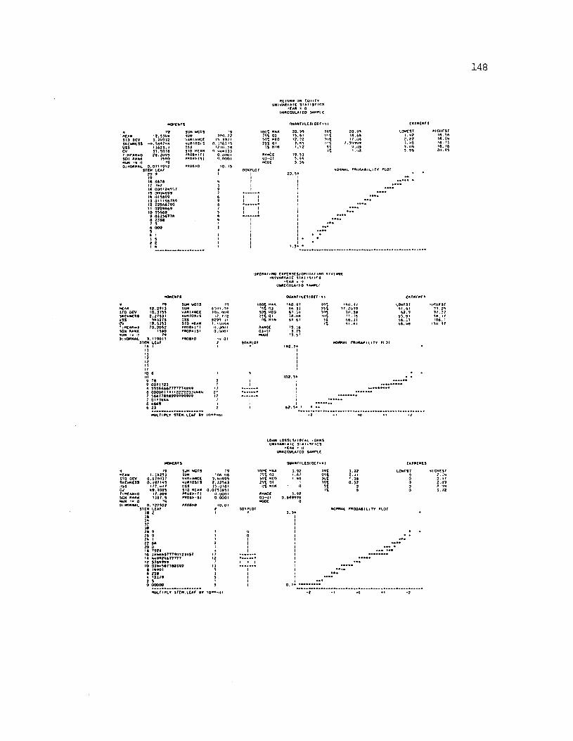
1 4 8

rtCMJMN ON CQIH (V UN IVAXI A / C S IA I IS M C S

'CAM « 0 UNftCCULA'CD U H F l C

NtANs r o o e v Snew ncS S u s sc vT : H ra n b Q SGH NANNHUM •« a 0:*0NMAL

1 2 .3 3 * * ) . ? * 9 1 2

• o . i f l A / u s 1 3 6 2 6 .*J t . 9 0 / 8 2 8 .2 U 9 9

I9 6 0 ’9

0 .0 7 1 1 9 * 2 S U M LCA7

20 9 1910 6 67#17 1*716 0 0 0 1 2 * 9 9 7 19 00U *699 19 0 1 1 6 9 9 IS 0 111967A 9 12 2 2 9 6 6 7 9 911 0 2 2 * * 6 9 10 1 9 6 6 99 03336776• 2 366 7 16 000 9• 1

SUM wetsSUMVANIANCC» u m o s i s: s sSIO NCANp*08x ri p n o n x s i

100'

1 2 1 0 .5 61 .U M K IJJ

0.0001'1.0001

MAX 79% 03 10% MCO 29% 01

0% MIN

NAHGC0 3 -0 1mooc

O U A N T H .C S IO r/''

2 0 .9 91 5 .3 11 2 .1 2

7 .3 9

1 9 .5 35 .7 65 .7 6

2 0 .9 9 16 . 69 I 7 .0 8

7 .3 * 9 9 9

NORMAL PN06A81 LI 7Y PLOT

i i t c n r s r 16 . 96 1 6 . fin

u p c n a m n g CxpC N SCS/O Pi'tA N N O n r v r w u n i v a n i a r c s i A i m t r s

'CAN • 'I U N X C r.u iA ito SAMfi.r

MCANs r o o c vSKCWNCSSu s sc vT: HCANbi) SON NANN ton *• 0 0 : KOXMAt.

8 2 .2 9 1 3■ 0 .3 1 9 92 .2 7 6 3 1

9 * 3 2 7 6> 2 .3 3 9 37 0 .9 0 9 2

i9 6 079

0 . 119011

sum w a r sSUMVANIANCC■ u N ro m sc s sSrO *(ANp n o s x r i/N O N A 'S '

M 0 6 > 0

6 " O l . f)1 106.<1119

i 2 . / : ? 929 9 11 ■ . if,0 8 6 II. IKK! I 0.0001

Til 01

>00% MAN M S 03 90% w co 25% 01

nanCC0 3 -0 1■*J0«

o u A N r a c s i o f r •

'* 0 .9 7 8 6 . 938 1 .3 *79.136 61 61

79 . 36 9- 79

7 1 .3 ’

9*>% 93% 7n% • n%

>111.4/ 7 7 .2 0 9 9

7 '1 . 96

(.OWfSr6 1 .3 1

8 2 .9 8 5 .9 1 9 6 . 31 66 . 46

ftONMAL PftfMAA t LI Tv P10 I

109 ?89 0 0 1 1 1 2 )6 3 5 3 6 6 6 6 7 7 7 9 7 7 6 9 9 96 OOOUOI1 tM 2 2 2 2 2 3 J * * * *7 3 6 6 7 7 9 6 8 9 9 9 9 9 9 9 9 9 7 0 1 1 3*0*6 6 6 6 9 6 2)

NULTI/t.7 STCN.LCAt #7 10

LOAM LO SSIS /rO TA L lOANS UN I VAN I A IC S IA ltS M C S

'CAN r | |UMNCCUlArCO SAMPLE

MCANs r o o c vSACWNCSS

r;MCAMaO SCN NANNHUM • • 0 0 : WON/ML

791 .3 * 2 9 3

o . 6 'n n j 7 0 .* 9 7 1 * 9

I 7 7 . ml 7 * 9 .9 0 6 9

1 7 .8 0 9 1 3 6 7 .9

7*0 .> 2 2 3 0 2

STEM LCA7 38 2

SUM WCTSSUMVANIANCt(U N fO SiSCSSs r o ncanpN 0 6 > « riPN OBXSI

P606>0

1 0 6 .0 6 0 . *11899 2 . 32963 3 9 . J 1 6 I

1 .0733691 0 . uQ 0 1 0 .0 0 0 1

*0.01

30% * c o29% 01 Ot M»*

itANce0 3 -9 1no oc

o u A N r t L t s i o c r . * !

3 .9 2 99%1 .6 / 99%'. « * 90%

1 10%0 9%

NONWAC PNQ0A6ILITV »L0?

2* >22 6*20 0 18 792616 3 * * * * 9 7 7 7 9 0 * 2 3 * 3 7 I* * * 9 * 2 1 6 7 7 7 7 7 12 9 7 8 9 9 9 9 10 0 3 * * 9 6 7 7 8 0 3 6 9 6 1*901 6 2281 723792 90 00000

NULTIP1.7 S f I M .L tA t 6V 1Q***<)»

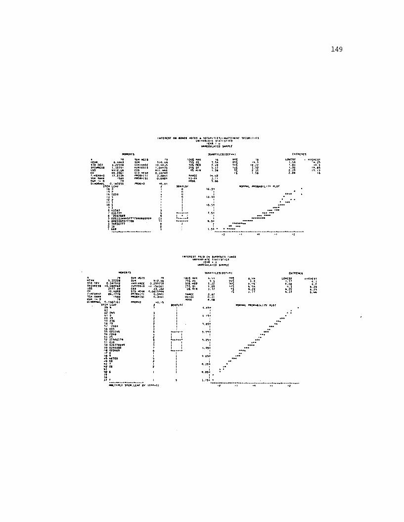
1 4 9

m rtN C S T o « oo n o s n o u s * s c r u m t i c s / s c c u r iUNIVANlAK S r A f 'S f lC S

* t* n ' u UftftCCULArCON C Msro ocv» ( M ( U

y \ n u m mum *« o0 : h o m w i

?9

1.225**1. J 9741* 1 1 2 .6 6*9 .69*1u . a u *

'930

sum v e r sSUMVANIAMCC HUM10313 CSSSIO Mf AM »«08>IT| **06>ISI**06»0

?90.167256

S U M LC*f 16 0 18 ?.1* 0 2 3 9 'I *>7 7 1 I 1 10 3 9 JS 0 3 3 6 7 7 0 3 6 7 7 7* 1 7 7 673693 0 2 2 1 3 1 * * * 3 7 7 7 7 8 8 6 6 8 3 9 9 9* 0 0 2 3 3 6 9 3 7 7 7 6 6 1 1»9367777 13 1 6 8 9

3 > 0 .66 10 - * 0 1*1 1.68*76 S I * . '<68 0 .J62N9

0.00*11 0 .0 0 0 1

1 0 0 t MAX79i ai90% MCO 29t atot MIN

NANGC0 1 -0 1MQOL

Q U A «T lt.CS(O Cr>li|

16 99tT.96 99%3.99 7*'t

I13.3*

I10.3*

II

7.3*I1

8.3*II

1.3* *

1 2 .7 7 1.32 2 .1 9 ■ 98 1.92

2.192 .3*

NORMAL MN06A0 IL< 77 *10r

INTCMCSr AAI0 ON 80*NOWCO IUNOS UMIVAftlAIC SIAIUI'CS

U A * ■ 3 U M C C U L A U O SAM*tf

Mf AN 3T0 OtV SHCWHC3S USSCVT:Mf AM»0 1CN AAR* NUM 0 OiNORMAL

799.22276

0.387912 ■ 0 .’1 * 0 0 6 2

2177.69 1 0 .* 8 * 2 3*.1778

193079

0.0967161 SU M ICAC 68 8

6162 089 91 9 60 *3 94 21696 >997 '2669 96 01)939 0211*998 226691 2992 2.9A67T4 91 01890 018 779394 89 0136669 '»* 021*69 <>7 0 86 993 86789 88 *9

SUM WCfS SUM/ANIANCC«u*rasisc s sSrO MfAN * * n * * i r i **06*191**OA>0

79* 12.96

0.299769 •«'. 190161

21.J82 7.0619499

0.0001 O.OtMJI

>*l. 13

30% MCO 291 atu t MIN

•AMCC0 1 -4 1m o o c

a u A u r iL C 9 io c r * * i

9.4 5 .2 2 *.34 1 . 77

2.67 0. 71 8 .9 6

I6. I9»I

9.39*I1

J !9*I

3.23*II

'*.95*II

8.63*II

6.13*1

*.03*{ •I

1. 73* •

6.2 9.'*6' 8.39

L0WCS7 1. 77 8.06 9.2

6.28 6.29 6. 8*

normal **0RA8»iinr *tor

WM.7IALV STCM.LCAf 3V 10**-0 I

Appendix B LIST OF BANKS IN SAMPLE

FIRST NB IN TUSCUMBIA AL 1976

UNIVERSITY NB OF FT COLLINS CO 1974 LAKEWOODCO NATIONAL BANK CO 1974FIRST NAT BK OF FRANKFORD DE 1973 FLORIDA NB AT GAINESVILLE FL 1976 FLAGSHIP BK OF MELBOURNE NA FL 1974 BARNETT BANK OF OCALA NA FL 1975FLGSHP 1ST NB OF VOLUSIA CTY FL 1973 HALIFAX NATIONAL BANK FL 1974GULF COAST NATIONAL BAK FL 1973INDUSTRIAL NATIONAL BANK FL 1973NATIONAL BANK OF GEORGIA GA 1976FIRST NB OF NEWTON CTY GA 1974FIRST NAT BK OF PAULDING CTY GA 1973 FARMERS NB OF MONTICELLO GA 1974FIRST NAT BANK OF VALDOSTA GA 1975 FIRST NB OF PRAIRIE CITY IA 1974CITIZENS NATIONAL BANK OF ID ID 1976 NATIONAL BANK OF ALEDO IL 1975EXCHANGE NAT BK OF CHICAGO IL 1973 NORTH SHORE NB OF CHICAGO IL 1973STEEL CITY NB OF CHICAGO IL 1975FIRST NB OF GENEVA I.L 1976FIRST NB OF LAKE BLUFF IL 1973FIRST NB OF METAMORA IL 1975NAT BK OF MONTICELLO IL 1976FIRST NAT BK OF RAYMOND IL 1975ROODHOUSE NATIONAL BANK IL 1975FIRST NB OF CLOVERDALE IN 1973FIRST NAT BANK OF GOODLAND KS 1976FIRST NAT BANK OF ONAGA KS 1974FIRST NAT BANK OF WAVERLY KS 1973FIRST NAT BK IN ARCADIA LA 1976CITIZENS NATIONAL BANK LA 1974FIRST NB IN ST MARY PARISH LA 1976FIRST NB OF BLOOMING PRAIRIE MN 1973FIRST PLYMOUTH NAT BANK MN 1973FIRST NAT BK OF CLAYTON MO 1973FIRST NB OF WEST PLAINS MO 1974FIRST NAT BANK OF PICAYUNE MS 1976PEOPLES BK OF MISSISSIPPI NA MS 1973 NATIONAL BANK OF HARVEY ND 1973

SANTA CLARITA NAT BANK W NB OF COLORADO SPRINGS FIRST NAT BK OF FLORENCE

CA 1974 CO 1974 CO 1976

NORTHWESTERN NB OF NORFOLK FIRST NAT BANK OF WALTHILL URBAN NATIONAL BANK UNTD JERSEY BK/MIDSTATE NA SANTA FE NATIONAL BANK FIRST NAT BK OF EAST ISLIP NATIONAL BANK OF MONTPELIER FIRST NATIONAL BANK YUKON NATIONAL BANK BLUE BALL NATIONAL BANK FIRST NAT BANK OF MAPLETON PEN ARGYL NATIONAL BANK FIRST NB OF SLIPPERY ROCK FIRST NAT BANK OF STRASBURG FIRST NAT BK OF GIBSON CTY FIRST NB OF RHEA COUNTY FIRST NAT BANK OF BELLVILLE BOWIE NATIONAL BANK CITIZENS NAT BK OF DALLAS HAMILTON NATIONAL BANK FIRST NAT BK OF HUNTSVILLE FIRST NAT BANK OF LEVELLAND FIRST NAT BANK OF MC GREGOR FIRST NAT BANK OF PLANO MOUNTAIN NB OF CLIFTON FORGE VA RICHLANDS NATIONAL BANK FIRST NAT BK OF TROUTVILLE RANDOLPH NATIONAL BANK UNIVERSITY NATIONAL BANK CTZ NB OF BERKELEY SPGS FIRST NAT BK OF WETUMPKA FIRST NAT BANK OF DAILY CITY CA PIKES PEAK NATIONAL BANK ROCK FORD NATIONAL BANK FARMERS NAT BANK OF AULT COLONIAL NATIONAL BANK CENTRAL NAT BANK OF MIAMI BARNETT BANK OF ST. PETERBRG FL BARNETT BANK OF CLEARWATER FIRST NB OF PUNTA GORDA ATLANTIC FNB OF DAYTONA BCH FIRST NB OF VOLUSIA CITY CITY NB OF HALLENDALE EAST FIRST NAT BANK FIRST NB OF COLUMBUS FIRST NAT BNK OF ALMA FIRST NB OF LOUISVILLE FIRST NB OF HOUSTON CITY CITIZENS NB OF QUITMAN FIRST NB OF WOODBINE FARMERS NAT BANK OF BUHL FIRST NB & TR OF CARBONDALE

NE 1976NE 1974NJ 1976NJ 1974NM 1973NY 1973OH 1973OK 1975OK 1973PA 1974PA 1976PA 1974PA 1973PA 1974TN 1976TN 1973TX 1974TX 1975TX 1976TX 1974TX 1974TX 1974TX 1975TX 1974VA 1975VA 1974VA 1974VT 1974WI 1975WV 1974AL 1976CA 1974CO 1974CO 1976CO 1974DE 1974FL 1973FL 1976FL 1974FL 1973FL 1975FL 1973FL 1974FL 1973GA 1973GA 1976GA 1974GA 1973GA 1973IA 1974ID 1975IL 1974

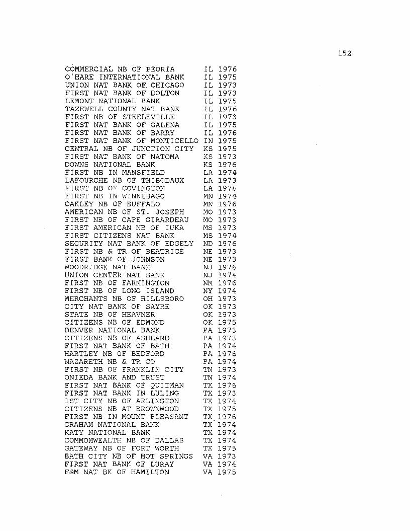
COMMERCIAL NB OF PEORIA O'HARE INTERNATIONAL BANK UNION NAT BANK OF. CHICAGO FIRST NAT BANK OF DOLTON LEMONT NATIONAL BANK TAZEWELL COUNTY NAT BANK FIRST NB OF STEELEVILLE FIRST NAT BANK OF GALENA FIRST NAT BANK OF BARRY FIRST NAT BANK OF MONTICELLO CENTRAL NB OF JUNCTION CITY FIRST NAT BANK OF NATOMA DOWNS NATIONAL BANK FIRST NB IN MANSFIELD LAFOURCHE NB OF THIBODAUX FIRST NB OF COVINGTON FIRST NB IN WINNEBAGO OAKLEY NB OF BUFFALO AMERICAN NB OF ST. JOSEPH FIRST NB OF CAPE GIRARDEAU FIRST AMERICAN NB OF IUKA FIRST CITIZENS NAT BANK SECURITY NAT BANK OF EDGELY FIRST NB & TR OF BEATRICE FIRST BANK OF JOHNSON WOODRIDGE NAT BANK UNION CENTER NAT BANK FIRST NB OF FARMINGTON FIRST NB OF LONG ISLAND MERCHANTS NB OF HILLSBORO CITY NAT BANK OF SAYRE STATE NB OF HEAVNER CITIZENS NB OF EDMOND DENVER NATIONAL BANK CITIZENS NB OF ASHLAND FIRST NAT BANK OF BATH HARTLEY NB OF BEDFORD NAZARETH NB & TR CO FIRST NB OF FRANKLIN CITY ONIEDA BANK AND TRUST FIRST NAT BANK OF QUITMAN FIRST NAT BANK IN LULING 1ST CITY NB OF ARLINGTON CITIZENS NB AT BROWNWOOD FIRST NB IN MOUNT PLEASANT GRAHAM NATIONAL BANK KATY NATIONAL BANK COMMOMWEALTH NB OF DALLAS GATEWAY NB OF FORT WORTH BATH CITY NB OF HOT SPRINGS FIRST NAT BANK OF LURAY F&M NAT BK OF HAMILTON

IL 1976IL 1975IL 1973IL 1973IL 1975IL 1976IL 1973IL 1975IL 1976IN 1975KS 1975KS 1973KS 1976LA 1974LA 1973LA 1976MN 1974MN 1976MO 1973MO 1973MS 1973MS 1974ND 1976NE 1973NE 1973NJ 1976NJ 1974NM 1976NY 1974OH 1973OK 1973OK 1973OK 1975PA 1973PA 1973PA 1974PA 1976PA 1974TN 1973TN 1974TX 1976TX 1973TX 1974TX 1975TX 1976TX' 1974TX 1974TX 1974TX 1975VA 1973VA 1974VA 1975

153FACTRY PT NB OF MANCHESTER VT 1974 FIRST NB OF PORT WASHINGTON WI 1974 FIRST NB OF KEYSTONE WV 1974

VITA

Robert Edward Lamy was born on December 28, 1953 in New Orleans, Louisiana to Gerard and Marie Lamy. After graduation from St. Paul's High School in Covington, Louisiana, he entered Southeastern Louisiana University and graduated in the Winter of 1974 with a B.S. degree in Marketing. He enrolled in the Graduate School at Southeastern Louisiana University and matriculated there from 1975 through 1976, receiving an M.B.A. degree at graduation.

In the Spring of 1978, he enrolled in the doctoral program at Louisiana State University and is scheduled to receive the Ph.D. degree with a major in Finance and a minor in Quantitative Methods in the Spring of 1984.

Mr. Lamy is currently an Assistant Professor of Finance at Virginia Polytechnic University and State University in Blacksburg, Virginia.

He is married to the former Amy Lynne Marchiz of New Orleans, Louisiana and they have one daughter, Meredith Margaret, and four dogs, Bubba, Eddie, Annie, and Toto.

154

EXAMINATION AND THESIS REPORT

Candidate:

Major Field:

Title ot Thesis:

Robert Edward Lamy

Finance

An Empirical Investigation of the Effect of Capital Structure Regulation on the Asset Portfolio of Commercial Banks

Approved:

X / yLMajor Professor and Chairman

l i i ■ / UDean of the Graduate ISchool

EXAMINING COMMITTEE:

A-vt-Q i :

Date of Examination:

March 9, 1984