The Effect of Electricity-Use Feedback on Residential Consumption: A Case Study of Customers with Smart Meters in Milton, Ontario

by

Jennifer Robinson

A thesis presented to the University of Waterloo

in fulfilment of the thesis requirement for the degree of

Master of Environmental Studies in

Environment and Resource Studies

Waterloo, Ontario, Canada, 2007

© Jennifer Robinson 2007

I hereby declare that I am the sole author of this thesis. This is a true copy of the thesis, including any required final revisions, as accepted by my examiners. I understand that my thesis may be made electronically available to the public. Jennifer Robinson

ii

Abstract Faced with a looming electricity crisis, the provincial government is calling for Ontarians

to adopt a “culture of conservation”, and is planning to equip all residential dwellings

with new metering infrastructure known as “smart meters” by 2010. In addition to

providing residents with the ability to “shift” their electricity consumption from the most

expensive “on-peak” times of the day, the data from these meters can be used to provide

residents with detailed information, or feedback, regarding their consumption patterns.

This research assessed whether electricity-use feedback affected households’ electricity

consumption behaviour, whether feedback effected pro-conservation attitude changes,

and what types of feedback were most effective in these regards. An initial mail survey

was sent to 1,257 smart metered Milton, Ontario homes to obtain information regarding

residents’ appliances and their consumption behaviour and attitudes. Of the 298

respondents, most of whom were living in homes that were less than seven years old, 106

were chosen to receive weekly household-specific feedback in various formats from July

to October 2006. A follow-up survey was conducted to assess any changes in attitude as

a result of the feedback, and weather-adjusted 2005 and 2006 consumption data were

used to quantitatively discern any resulting consumption changes. While overall results

revealed that the feedback made little difference in household consumption levels

compared to the 2005 baseline period, there were some indications that it was effective in

encouraging shifting, and had the opposite effect on overall conservation (i.e. it

encouraged increased consumption). Also, while the comparison of “pre-” and “post-

feedback” surveys revealed the feedback had no measured effect on encouraging pro-

conservation attitudes, overall, customer acceptance of the feedback was high.

iii

Acknowledgments I am very much appreciative of the support and guidance that Dr. Ian H.

Rowlands, my thesis advisor, has provided me throughout my time in the University of

Waterloo’s Master of Environmental Studies programme. While never controlling, his

advice was always targeted, substantive, and delivered with humility and humour. He

was also fantastic at providing me, as well as his other students, with great opportunities

to showcase our research.

We could not have asked for better industry partners than Don Thorne, President

and CEO, and Mary-Jo Corkum, Vice President of Finance at Milton Hydro Distribution

Incorporated. The time and resources they dedicated to the project, not to mention their

enthusiasm and support, made working with them a joy (at the risk of sounding

effusive!). I would also like to acknowledge Andrew Peers and Drazen Prodanovic, who

were always quick to respond to my multiple data requests. I owe a lot to Cathy

Mandarino as well, who spent a substantial amount of time inputting survey data for me.

I am grateful for the funding I received from Canada’s Social Sciences and

Humanities Research Council, and I would like to acknowledge the Centre for Energy,

one of the Ontario Centres of Excellence, which also funded this work and provided me

with opportunities to present the research externally.

I am very appreciative of Bijan Alagheband and Stan But at Hydro One Networks

Incorporated as well, who weather-adjusted all of our data, and always did so

expeditiously.

Erin Harvey and her army of statistical consultants at the University of Waterloo’s

Statistical Consulting Service were also instrumental in helping me choose the

appropriate statistical design and testing for this research. Mary Thompson of the Survey

Research Centre gave fantastic advice regarding the design of my survey instruments.

Both Erin and Mary were wonderful at always finding the time to fit me in to address my

endless questions.

Megan Conway volunteered her editing skills and great advice during the final

throes of my writing process, for which I am also very much appreciative.

Finally, a big thank you goes to all my family and friends who have been so

supportive of me during my time at the University of Waterloo.

iv

Table of Contents Abstract .............................................................................................................................. iii Acknowledgments.............................................................................................................. iv Table of Contents................................................................................................................ v List of Tables .................................................................................................................... vii List of Figures .................................................................................................................. viii 1 Introduction................................................................................................................. 1

1.1 Research Contributions....................................................................................... 3 1.2 Target Audience.................................................................................................. 4 1.3 Study Site ............................................................................................................ 4

2 Study Context: Residential Energy Use Behaviour .................................................... 7

2.1 Attitudes and Behaviour ..................................................................................... 7 2.2 Energy Consumption Behaviour Interventions................................................... 9 2.3 Feedback ........................................................................................................... 13 2.4 Research Gaps................................................................................................... 26 2.5 Research Conceptual Framework ..................................................................... 27

3 Methodology............................................................................................................. 32

3.1 First Survey (May 2006)................................................................................... 33 3.2 Feedback Testing (July to October 2006)......................................................... 34 3.3 Second Survey (November 2006)..................................................................... 45 3.4 Overall Research Metrics – The Dependent Variables..................................... 47 3.5 Overall Research Design Limitations ............................................................... 51

4 Results....................................................................................................................... 54

4.1 Survey #1 Results: Context for the Study........................................................ 54 4.2 Electricity Consumption Data – Pre- and Post-Feedback Results .................... 66 4.3 Survey #2 Results ............................................................................................. 77

5 Analysis..................................................................................................................... 86

5.1 Pre- and Post-Feedback Consumption Data Analyses...................................... 86 5.2 Pre- and Post-Feedback Survey Analyses....................................................... 107 5.3 Other Findings from Survey #2 ...................................................................... 108

6 Conclusions............................................................................................................. 110

6.1 Comments on Relevant Theories .................................................................... 110 6.2 Broader Study Implications and Recommendations....................................... 112 6.3 Future Work .................................................................................................... 114

References....................................................................................................................... 115

v

Appendix I Survey #1 ............................................................................................ 122 Appendix II Feedback Examples ............................................................................ 131 Appendix III AC Usage Calculation Methodology.................................................. 137 Appendix IV Environmental Metric Examples ........................................................ 139 Appendix V Group Similarity Testing .................................................................... 141 Appendix VI Survey #2 ............................................................................................ 143 Appendix VII Survey #1 Results Tables.................................................................... 154 Appendix VIII Weather-adjusted Consumption Results ............................................. 198 Appendix IX Normality Results ............................................................................... 211 Appendix X Mann-Whitney Results for Treatment and Control Groups ............... 216 Appendix XI Two-Way Univariate ANOVA Results .............................................. 220 Appendix XII Kruskal-Wallis Results ....................................................................... 224 Appendix XIII Survey #2 Results Tables.................................................................... 230 Appendix XIV Plots of Significant Dependent Variables ........................................... 263

vi

List of Tables Table 1 – Literature Rationale for Testing Independent Variables with Feedback .......... 37 Table 2 – Feedback Testing Design Variables and Sample Sizes .................................... 42 Table 3 – Survey Respondent Screening Criteria ............................................................. 45 Table 4 – Baseline and Test Periods ................................................................................. 48 Table 5 – Consumption Data Analysis Dependent Variables........................................... 50 Table 6 – Demographic and Structural Comparisons of the First Survey Respondent Base

to the Greater Town of Milton and the Province of Ontario..................................... 56 Table 7 – “What does a ‘conservation culture’ mean to you?” ........................................ 61 Table 8 – Adjusted Control and Treatment Group Sizes.................................................. 68 Table 9 – Weather-adjusted Consumption Values – Group Averages ............................. 69 Table 10 – Dependent Variables Found to be Normal, All Treatment Groups (no CGs) 71 Table 11 – Mann-Whitney Testing for Consumption Changes Comparing All Treatment

Groups and Control Group 3 – Significant Results Only ......................................... 73 Table 12 – Mann-Whitney Test Results For Consumption Changes Comparing All

Treatment Groups to Control Groups 1 and 2 – Significant Results Only ............... 74 Table 13 – Mann-Whitney Test Results For Consumption Changes Comparing All

Treatment Groups and All Control Groups – Significant Results Only ................... 75 Table 14 – Two-Way Univariate ANOVA Testing – Significant Results Only............... 76 Table 15 – Kruskal-Wallis Test Results for Independent Variable Effects – Significant

Results Only.............................................................................................................. 76 Table 16 – Attitudinal Question (From First and Second Survey) and Ranking Value ... 79 Table 17 – Mann-Whitney Test Results for Self-Reported Changes Comparing Feedback

Recipients and Non-Recipients................................................................................. 80 Table 18 – Comparison of Conservation-related Attitudes and Behaviours of the

Treatment and Control Groups ................................................................................. 87 Table 19 – Treatment and Control Group Comparisons – All Significant Findings ........ 93 Table 20 – Comparison Significant Finding Summary .................................................. 101 Table 21 – Mail versus Email Behaviour ....................................................................... 105 Table 22 – Summary of Study Findings ......................................................................... 111

vii

List of Figures Figure 1 – Location of Milton, Ontario, Canada ................................................................ 4 Figure 2 – Electricity Consumption Feedback Conceptual Framework........................... 28 Figure 3 – “How would you rate your awareness of your home’s specific electricity

consumption levels?” ................................................................................................ 58 Figure 4 – “Do you feel that you know enough about your home’s electricity

consumption to decide how to best conserve electricity?” ....................................... 58 Figure 5 – “Are you satisfied with the layout and information provided on your electricity

bill?”.......................................................................................................................... 59 Figure 6 – “Please indicate your household’s commitment to conserving electricity.” ... 59 Figure 7 – “Have you heard of any of the following?”..................................................... 60 Figure 8 – “What motivates you to conserve electricity in your home?” (ranking question

with 7 choices) .......................................................................................................... 62 Figure 9 – “Please indicate your household’s level of commitment to reducing your ‘on-

peak’ electricity use.”................................................................................................ 63 Figure 10 – “Do you use compact fluorescent light bulbs?” ............................................ 64 Figure 11 – “Do you have plans to do any of the following in the next 2 years?”........... 65 Figure 12 – “How often do you have conversations about energy conservation with the

following people?”.................................................................................................... 66 Figure 13 – Salience of Feedback Features ...................................................................... 83 Figure 14 – “What was your reaction to knowing how much CO2 you saved/increased

compared to the previous summer in terms of the equivalent number of car trips to Toronto?” .................................................................................................................. 84

Figure 15 – Various Opinions on the Emissions-related Information Provided............... 85

viii

1 Introduction Ontario’s power infrastructure is in a critical state. Approximately two-thirds of its

current generation capacity, most of it nuclear, will reach the end of its planned operating

life by 2025. Factoring in the growing economy, as well as the provincial government’s

commitment to phase out coal-fired generation in response to the growing public demand

to reduce greenhouse gases and air pollution, the proportion of generation facilities that

will need to be replaced or refurbished by 2025 climbs to 80% (Ontario Power Authority,

2005). Amidst this climate, business and industry, still haunted by the turbulent effects

of the August 2003 blackout on the economy, are demanding reliability of supply and

cost stability in order to maintain competitiveness.

Given the 40 billion Canadian dollar estimated cost of the required generation

investments (Hamilton, 2007), it is widely recognized that less costly electricity

conservation programs must play an essential role in the province’s infrastructure

development plans. In 2004, the province established a Conservation Bureau to lead the

effort in developing a “culture of conservation” in Ontario (Government of Ontario,

2005).

While this definition remains unclear (Enbridge Gas Distribution, 2007), it is believed

that the term “conservation”, as used in the term “conservation culture”, encompasses

behaviours such as conservation (i.e. overall consumption reduction by using less), as

well as “shifting” from “on-peak” times (i.e. using less electricity during the hours of the

day when electricity demand is highest), and even energy efficiency (i.e. consumption

reduction by using more highly efficient technologies). Also, the term “culture” implies

behaviour as well as attitudes. For the purpose of this research, a conservation culture

has been defined as an exhibition of both pro-electricity-conservation behaviour and

attitudes. Furthermore, both conservation and shifting behaviours and attitudes will be

examined.

1

It can be argued that households will be important contributors in the development of a

conservation culture in Ontario. Average household electricity consumption in the

province is only slightly lower than the Canadian average (Aydinalp, Fung, & Ugursal,

2000), and Canadian households are among the highest per-capita electricity consumers

in the world (Energy Information Administration, 2006). Furthermore, Ontario

households consume one-third of the province’s electricity (Ontario Energy Board,

2005). As one means of providing the residential sector with the tools for electricity

consumption reduction, the province plans to equip all households with “smart meters”

by 2010. In Ontario, smart metering involves technology that will be capable of

recording electricity consumption and the time at which it occurs, which will in turn

allow regulators to set electricity prices that better reflect market prices that vary

throughout the day. During the summer months, electricity demand and prices are the

highest on weekdays during the day (i.e. during on-peak periods); on weekday evenings,

both demand and price drop (i.e. during “mid-peak” and “off-peak” periods). During the

winter months, on-peak demand occurs on weekdays in the morning and evening.

This dynamic pricing scheme is known as “time-of-use” pricing and it represents a

significant departure from the conventional tiered pricing scheme, under which residents

essentially pay a flat rate per unit of consumption up to a certain threshold level. Smart

meters will thus ostensibly encourage electricity consumers to take advantage of price

savings by shifting their usage from on-peak periods. This shifting will aid in

“smoothing” the province’s load profile and should result in lower on-peak capacity

requirements, thus potentially reducing new generation investment requirements. This

smoothing should lower electricity prices as well, as there will be less demand for

electricity supplied during the costliest period of the day.

To further encourage residents to respond to time-of-use pricing, Ontario’s infrastructure

will also provide residents with the capability of viewing their own electricity

consumption details within 24 hours of consumption. This information, which represents

the consumers’ past consumption behaviour, is a form of “feedback”. This information

will likely be made available via websites or over the phone (Smart Meter Ontario, 2007).

2

Feedback information pertaining to actual household electricity-use has been shown to be

effective in inducing energy consumption behavioural change (Darby, 2000; Fischer,

2007; Seligman, Becker, & Darley, 1981; Wood & Newborough, 2003). Although a

significant amount of research has been performed relating to electricity consumption

feedback, some of it in conjunction with time-of-use pricing, much of this dates back to

the late 1970s and early 1980s (e.g. Heberlein & Warriner, 1983). Although there is

more recent work assessing the effectiveness of time-of-use (and other) pricing schemes

in California (George & Faruqui, 2005), as well as some feedback-related research within

the California context (Martinez & Geltz, 2005), it is not known how these findings will

translate to the Ontario context, particularly due to the province’s relatively low

electricity price environment. An initial Ontario-based smart metering pilot assessment

concentrated on the impact of time-of-use pricing, but not specifically on feedback (IBM,

2007).

As the Ontario smart meter deployment will be one of the largest in North America, it

can be argued that there is a need to understand how the electricity-use information that it

will make available can be used to encourage consumption behavioural change.

This research therefore aims to answer the question: “How are electricity consumption

behaviour and attitudes of selected customers with smart meters influenced by residential

electricity-use feedback information in Milton, Ontario?”

1.1 Research Contributions

From a practical perspective, this research provided insight into the type of feedback that

would be successful in bringing about changes in consumption behaviour in an Ontario

urban context. It also provided insight as to whether feedback affected consumers’

attitudes towards electricity conservation issues, which may help to further motivate

individuals to exhibit conservation behaviour.

3

From an academic perspective, this research contributed empirical evidence to the bodies

of work describing various behavioural interventions, particularly as they relate to the use

of feedback.

1.2 Target Audience

It was expected that this study would be of significance to program developers at local

electricity distribution companies, community-based organizations and smart metering

system developers servicing Ontario. The findings may also be useful in contributing to

policy development at the provincial level in Ontario, as well as in other jurisdictions that

may be considering smart metering technology. Lastly, the findings may also translate to

other resource management sectors interested in consumption behaviour, such as those

involved with water demand management strategies.

1.3 Study Site

The town of Milton, Ontario, situated approximately 55 kilometers west of Toronto

(Figure 1), is currently undergoing a period of rapid growth. In 2006 its population was

approximately 54,000, which was a 70% increase from 2001, the last census year.

Figure 1 – Location of Milton, Ontario, Canada

Source: Town of Milton, n.d.

4

It is partly due to this growth that Milton became one of the first jurisdictions in Ontario

to have initiated significant smart meter installations, mainly in newly constructed homes.

Milton Hydro Distribution Incorporated is recognized as a leader in conservation efforts

province-wide, and their willingness to engage in progressive conservation research,

coupled with the availability of some of the first detailed smart metering electricity

consumption data in the province, were the key reasons for the selection of Milton as the

research site. Led by Professor Ian Rowlands, the Faculty of Environmental Studies at

University of Waterloo has developed a formal partnership with Milton Hydro that is

funded with support from the Ontario Centres of Excellence.

Within Milton, the study focused on a sub-set of households that has been equipped with

smart meters since at least May 2005, so that adequate baseline data was available for the

study. The baseline period was August to October 2005, and the test period, when

residents were provided with the feedback intervention, was from August to October

2006.

This introduction has sought to provide a rationale for the need for research relating to

residential electricity-use feedback in the Ontario-specific context. Chapter 2 follows,

which provides an overview of the academic literature from the past three decades

relating to the relationships between attitudes and behaviour, and the experience with

energy conservation intervention strategies, with a specific focus on the functions and

effectiveness of feedback. The chapter ends with a discussion of some of the research

gaps in the literature, and attempts to synthesize the findings with of a conceptual

framework that can be used to understand the functions of feedback as explained by

various attitudinal and behavioural theories. Chapter 3 then lays out the research design,

and explains how the methodological instruments, a pre- and post-feedback survey, and

the feedback instrument itself, were developed and used. Chapter 4 provides an overview

of the results of the surveys, as well as the changes in consumption levels over the course

of the test period relative to the baseline period. Various statistical tests are applied to

these data as well, which are analyzed in detail in Chapter 5. Finally, Chapter 6

5

concludes the study by offering a summary of the results and their analysis, followed by

their potential policy implications; related future work is also discussed.

6

2 Study Context: Residential Energy Use Behaviour This research centres on electricity consumption feedback information, and its potential

to effect behavioural and attitudinal change, and as such, this review considers the

existing body of research that links these topic areas. It begins with a review of literature

from the past three decades that explores the relationship between attitudes and

behaviour, and presents various intervention strategies designed to encourage

conservation behaviour. It then examines feedback, one specific energy conservation

intervention strategy, in more detail by considering the mechanisms by which feedback

works, the criteria for effective feedback, and the potential limitations of using feedback

to promote conservation. Research gaps are highlighted, and the whole review is then

summarized through the presentation of a conceptual framework that suggests a proposed

relationship amongst the aforementioned topics and the relevant theories that have been

used to underpin past research, and, indirectly, this research as well. A discussion of the

interaction between attitudes and behaviour will now be presented.

2.1 Attitudes and Behaviour

A significant body of research has been dedicated to understanding the relationship

between attitudes and behaviour, and specifically the degree to which the former may

predict the latter. This predictive nature has long been recognized as being somewhat

tenuous (Brandon & Lewis, 1999; Gatersleben, Steg, & Vlek, 2002; Hutton, Mauser,

Filiatrault, & Ahtola, 1986; Kantola, Syme, & Campbell, 1984; Poortinga, Steg, & Vlek,

2004). Reasons for the low attitude-behaviour link can be related to knowledge and

awareness levels. Gatersleben et al. (2002), through the results of two large-scale surveys

of Dutch households, showed that, among other things, households with high pro-

environmental attitudes were often not aware of the environmental impacts of their

energy consumption, both directly and indirectly. Darby (2006) argues that behaviour

that is not keeping up with increasingly pro-environmental attitudes may be due in part to

an inability of individuals to link their specific actions to the overall impact. Another

potential reason for the low attitude-behaviour link is that studies often fail to take into

account external factors beyond the householders’ control. Guagnano, Stern, and Dietz

7

(1995) report evidence that attitudes toward recycling can in fact predict recycling

behaviour when external factors such as convenience levels are taken into account.

Kaiser, Wolfing, and Fuhrer (1999) also argue the need to take into account contextual

factors, and believe that the seemingly weak attitude-behaviour link supported by past

studies may relate to differing definitions of attitudes.

Despite this, some research has shown that attitudes can in fact predict behaviour.

Although Scott (1999) found that the attitudes of people who recycled were wide-

ranging, he did note that those with the lowest pro-environmental attitudes tended to

recycle less. Heberlein and Warriner (1983) found that the knowledge and the “conative”

component of attitudes (defined as the intention to act) were stronger predictors of

householders’ shifting electricity use from on-peak times than were price incentives and

appliance stocks. Rowlands, Scott, and Parker (2000) found a weak positive correlation

between general pro-environmental attitudes and self-reported home energy conservation

measures, with a slightly higher positive correlation between climate change attitudes and

conservation measures. This corresponds with other research that argues that attitudes

can better predict behaviour once they become more specific (e.g. Gatersleben et al.,

2002; Kaiser, Wolfing, & Fuhrer, 1999). Wilson and Dowlatabadi (2007) and

Gatersleben et al. (2002) reviewed past research that has found that attitudes can be

useful in predicting behaviour relating to the curtailment of simple measures, or

behaviour that does not have a high financial or psychological impact on people’s daily

lives such as energy use.

There are also cases where behaviour changes have resulted in attitude changes that can

lead to longer-term or sustained behavioural change. One meta-analysis indicates that

interventions aimed at attitude change may directly impact behaviour only weakly in the

short term, but may be beneficial for longer-term change (e.g. in the form of building

political support for change, etc.) (Wilson & Dowlatabadi, 2007). Dwyer, Leeming,

Cobern, and Jackson (1993) also argue that attitude change is important for sustained

behavioural change. Van Houwelingen and van Raaij (1989) propose that small

8

behaviour changes can eventually lead to habit formation and ultimately attitude change

as individuals adjust their attitude to reflect their new behaviour.

Attitudes as well as behaviour were considered in this study as they were both considered

to be requisite components of the “conservation culture” that Ontario is seeking. This is

because, although ultimately behaviour change in terms of reductions in total and on-

peak electricity consumption is important, there is literature that supports the need for

attitudinal change as well to help encourage initial behaviour change, and perhaps more

importantly, to sustain behaviour change over the long term.

The following section concentrates on the behavior component of the “conservation

culture” by considering the relative success of the various behaviour intervention

strategies that have been implemented over the years.

2.2 Energy Consumption Behaviour Interventions

The body of research considering the correlation between attitudes and behaviour

discussed above also often includes empirical studies relating to the effectiveness of

various interventions to encourage conservation behaviour at the household and

individual levels. It should be noted that, while this study is concerned with conservation

as well as the shifting of electricity use patterns, most of the intervention literature

reviewed is concerned mainly with conservation. However, much of the past work is also

relevant to the concept of shifting as well.

Energy conservation interventions can be categorized in various ways, and the taxonomy

employed varies depending on the researchers (e.g. Abrahamse, Steg, Vlek, &

Rothengatter, 2005; Dwyer et al., 1993; Guerin, Yust, & Coopet, 2000; Katzev &

Johnson, 1987; Winett & Ester, 1983; Wood & Newborough, 2003). For the purpose of

this review, the most frequently used categories of “antecedent” and “consequence” will

be used. The following offers a summary of the different types of antecedent and

consequence strategies and some of the results of their deployment.

9

2.2.1.1 Antecedent Interventions

Antecedent strategies refer to interventions designed to prevent (or encourage) specific

future behaviours (i.e. they target behaviour before it occurs). They can include

information campaigns (e.g. conservation campaigns, books, pamphlets, workshops,

etc.); prompts, which are generally shorter and less detailed than information campaigns

(e.g. cues to spark conservation behaviour, posters, flyers, etc.); and persuasion tactics

(e.g. comprehensive marketing campaigns, messages stressing personal gain and societal

benefit, letters to owners stating their conservation levels are not in line with their

environmental values, etc.).

Overall, Katzev and Johnson (1987) suggest that antecedent strategies can be fairly

limited in terms of conservation impact, and that an information approach alone is not

effective in bringing about significant and sustained behaviour change. Other researchers

assert that too often information campaigns have failed because not enough attention was

paid to using psychological techniques to ensure the audience adequately receives the

message (Stern, 1992). If done properly, some argue they can be beneficial, particularly

in conjunction with other techniques (Abrahamse et al., 2005 citing van Houwelingen &

van Raaij, 1989).

Although feedback, the intervention used in this particular study, is primarily considered

a consequence intervention (described below), it can be regarded as a type of antecedent

intervention as well, as it represents an opportunity to provide consumers with general

information regarding energy conservation. Indeed, Darby states that “information and

feedback are needed for maximum effectiveness” (2006, p. 2937, emphasis in original).

Other reviews echo this finding (Fischer, 2007), and more about the types of information

that have been found to be effective when offered with feedback will be discussed below.

However, feedback is first and foremost a type of consequence intervention, and a review

of the research relating to these types of interventions follows.

10

2.2.1.2 Consequence Interventions

Consequence strategies are designed to reward, penalize, or inform individuals based on

their behaviour after it occurs so as to potentially influence future behaviour. As per

Wood and Newborough, the strategy “relates directly to a consumer’s behaviour, i.e. it is

feedback that provides a user with information about the action he/she has carried out (or,

more succinctly, knowledge of results)” (2003, p. 823). While this definition obviously

includes feedback as a type of consequence strategy, other consequence strategies include

incentives and commitment strategies.

Incentives are conservation-related monetary rewards or prizes, and disincentives are

costs, penalties, or inconveniences. Examples of this latter point include traffic jams,

slowing elevator times, and higher electricity prices during certain times of the day.

Incentive research has reported a series of positive results (see Abrahamse et al., 2005 for

a review), but conclusions regarding the overall effectiveness of incentives are not

unanimous. When financial incentives were offered to a sample of similar households

(i.e. from the same geographic area), the amount of investment that took place varied

tenfold (Stern, Aronson, Darley, Hill, Hirst, Kempton, & Wilbanks, 1986). One

explanation for this is that those who have made some sort of a commitment such as

requesting an energy audit are more likely to make investment. Thus, incentives do little

to overcome initial barriers such as requesting audits. There is also the concern of the

“free rider” phenomenon of incentives predominantly being used by those who likely

would have taken the conservation action anyway (Ontario Power Authority, 2006). In

addition, incentives do not always lead to reduced consumption, and their effect can be

reduced once the incentive has been removed (Abrahamse et al., 2005; Cook &

Berrenberg, 1981; Katzev & Johnson, 1987). The programs can also be expensive, and

they can be complicated by the fact that their appeal will vary depending on the target

group, as well as by other factors such as “[a]dministrative effort, eligibility criteria, cash

flow timing, the relevance of immediacy… and the requirement to take on debt” (Wilson

& Dowlatabadi, 2007, p. 28). Regarding time-of-use pricing, which is a sort of incentive

to encouraging consumption during off-peak times, Heberlein and Warriner (1983) found

11

that it was effective in encouraging shifting, but that attitudinal components actually had

a much larger effect on shifting.

Broadly speaking, written or verbal commitment strategies can have “considerable”

(Katzev & Johnson, 1987, p. 123) impact on motivating people to conserve energy. One

study that distributed conservation information found that asking some residents to

commit to filling out a small questionnaire or to making an explicit conservation

commitment of 10% resulted in a higher overall savings compared to the control groups

who also received the conservation information (Katzev & Johnson, 1983). Also,

commitment interventions have been found to result in conservation even beyond the

intervention period. One study found that the beneficial effects of making public

commitments regarding gas and electricity conservation still existed six months after the

intervention (Abrahamse et al., 2005 citing Pallak & Cummings, 1976). From a sample

of households who took part in a conservation study, those who agreed to have their

name published as having taken part in the study resulted in an electricity savings of 20%

and a natural gas savings of 15%. Furthermore, this savings was still present one year

later (McKenzie-Mohr, 1994). Goal-setting is an explicit form of commitment, and this

has also been extensively studied in the context of household energy conservation. One

meta-analysis cited a 20% energy savings when households were asked to take on an

explicit conservation goal (Winett & Ester, 1983 citing Becker, 1978). As will be

discussed further below, some feel that feedback is effective mainly if it is combined with

some sort of explicit goal-setting function (Seligman et al., 1981).

A discussion of incentives and commitment strategies is relevant to this study for several

reasons. In the case of incentives, all households in the study were being charged time-

of-use rates during the test period, and as such were being provided with an incentive to

shift their consumption from on-peak periods. (As will be described in Chapter 3, this in

some ways confounds the effect of the feedback, but this was addressed through the use

of appropriate control groups.) In the case of commitment and goal-setting strategies, the

relevance to the study is more indirect: household consumption levels were reported

12

relative to a specific standard, the purpose of which was to provide a frame of reference

and in some cases an indirect attainment goal.

The feedback itself, another consequence intervention strategy and the main focus of this

study, will now be discussed in more detail.

2.3 Feedback

Feedback is defined as “[t]he modification, adjustment, or control of a process or system

(as a social situation or a biological mechanism) by a result or effect of the process, esp.

by a difference between a desired and an actual result; information about the result of a

process, experiment, etc.; a response.” (Oxford University Press, 1989). In the context of

energy consumption research, it can be categorized as direct (e.g. in-home displays,

consumption limiters, pre-payment schemes), indirect (e.g. utility bills and information)

and inadvertent (e.g. energy audits) (Darby, 2000).

In the past, some researchers have stated that its use is over-prescribed (Katzev &

Johnson, 1987). One study found that in-home displays offered no overall conservation

savings, although they did slightly encourage shifting (Sexton, Johnson, & Konakayama,

1987). Winett, Kagel, Battalio, and Winkler (1978) found that feedback was not useful in

encouraging air conditioning load reduction during summer periods, although high

rebates were. Another feedback study reported an effect that was opposite to what was

intended for low and medium consumers (i.e. those who received the feedback consumed

more than those who did not) (Bittle, Valesano, & Thaler, 1979-1980).

However, a significant body of research exists that supports its utility as well. One oft-

quoted meta-analysis reviewed 38 feedback studies covering various types of feedback,

and concluded that, on average, these techniques could bring about consumption

reduction in the order of 10% (Darby, 2000). Similarly, another individual study which

compared identical homes found feedback resulted in a 10% decrease in electricity

consumption (Guerin et al., 2000 citing Seligman & Darley, 1977). Comparative

feedback on air conditioning consumption resulted in a 20 to 30% electricity reduction

13

(McKenzie-Mohr, 1994). In households that received daily reports on projected monthly

energy consumption based on meter readings, consumption was reduced by

approximately 10 to 15% (Stern, 1992 citing Seligman et al., 1981). Another meta-

analysis cites feedback conservation studies resulting in consumption savings of 15%,

and as high as 30% during seasonal peak-use periods (Winett & Ester, 1983 citing

Seligman & Darley, 1977). A comparison study that pitted antecedent information

against feedback displays on electric stoves demonstrated average electricity savings of 3

and 15% respectively (Wood & Newborough, 2003).

Explanations of the results of the empirical work are often as varied as the results

themselves. In addition to pro-environmental or pro-conservation attitudes sometimes

being found to be determinants of conservation effects as has already been discussed,

demographic features such as household income have been studied as well. Some

research has argued a positive correlation between income and household consumption

levels (e.g. Gatersleben et al., 2002; Guerin et al., 2000 citing Heslop, Moran, &

Cousineau, 1981, Hines, Hungerford, & Tomera, 1986, Morrison, Gladhart, Zuiches,

Keith, Keefe, & Long, 1978, Newman & Day, 1975, and Ritchie, McDougall, & Claxton,

1981), although some has found that the link is not always clear (Brandon & Lewis,

1999). In terms of income and consumption level reductions as a result of feedback (or

other) interventions, again, some have found a positive correlation to exist (e.g. Guerin et

al., 2000 citing Eichner & Morris, 1984; Wilhite & Ling, 1995), while others have not

(e.g. Brandon & Lewis, 1999; Guerin et al., 2000 citing Johnson-Carroll, Brandt, &

Olson, 1987).

A discussion of feedback as a conservation intervention (and indeed this entire study) is

relevant because, as previously discussed, the Ontario smart meter deployment will result

in the unprecedented availability of detailed information for each consumer regarding

their consumption levels and patterns. For the purpose of this research, the effect of

providing indirect feedback in the form of weekly household-specific consumption

information was studied, as it was hoped that the research would highlight the type of

information that was most useful to the consumer, if any, and that resulted in the largest

14

consumption behaviour change. The body of research which examines the effects of

various types of feedback on electricity conservation efforts will now be reviewed in

more detail.

2.3.1 Feedback Mechanisms

The majority of feedback-related conservation research has spanned the last three

decades, dating back to the first oil embargo of the early 1970s. Since this time, different

explanations of the feedback effect as it relates to energy consumption behaviour have

been suggested.

Seligman et al. (1981) provide an excellent overview of a range of concepts or

approaches that attempt to describe how feedback may work. They dismiss the human

factor approach, which regards feedback as “primarily the teaching of new, skilled

responses” (Seligman et al., 1981, p. 100), as they argue that individuals generally know

how to reduce electricity consumption (e.g. turning off lights will reduce electricity

consumption; raising the temperature on the air conditioner will reduce electricity

consumption, etc.). Which appliances have the potential to produce the greatest savings,

and whether the motivation exists to conserve are of course important, but these are not

explained with the human factor approach.

The reinforcement approach considers feedback as a type of reward (or punishment) in

and of itself. Seligman et al. (1981) argue that this may not necessarily apply either, and

use empirical evidence that suggests individuals acted to save energy with the help of a

specific prompt (a light flashing when their air conditioning was on, but temperatures

outside were cool enough to not warrant the use of the air conditioning), and that

subsequent feedback (in the form of a hard copy of their actual consumption levels) was

effectively ignored. While this supporting evidence can be disputed on the basis of

various confounding effects (i.e. the flashing light, also a type of feedback, occurred in

real-time whereas the paper feedback only occurred three times a week; the validity of

the paper feedback was questioned by the individuals), the point remains valid: the

feedback itself, numbers or charts on a piece of paper, may not be a significant reward,

15

save in cases where it can lead to feelings of happiness for achieving a goal. While it is

true that feedback can highlight electricity savings and therefore monetary savings, the

feedback is the “messenger”, not the reward itself.

The motivational approach suggests that feedback acts to motivate individuals to

conserve. Seligman et al. (1981) argue that it is “highly unlikely that feedback in itself is

motivating in the sense of supplying a person with the drive to conserve energy” (p. 104).

Further to this explanation, it can be argued that feedback may serve to expose pre-

existing motivations, even those that an individual may not know exist. Such motivations

may include a desire to save money, a desire to behave in accordance with an individual’s

strong conservation ethic, a desire to achieve a goal, a desire to be perceived socially as a

conserver, etc.

Seligman et al. (1981) end their descriptions of how feedback can potentially lead to

increased conservation efforts by explaining the approach which they feel best explains

the phenomenon: feedback works by “showing that actual conservation is below the level

the person wants to achieve” (p. 105). In other words, individuals who have a

conservation goal will use feedback to assess their performance with respect to that goal.

Seligman et al. (1981) further explain this theory by using empirical examples whereby

households were asked to take on explicit conservation goals whose attainability varied

from easy to difficult. Those that were given the most difficult goals conserved the most

electricity, whereas those that were given easy or no goals had insignificant electricity

savings. While Seligman et al.’s (1981) examples imply explicit goal-setting should be

involved to obtain a conservation effect from feedback, they also cite Locke, Cartledge,

and Koeppel (1968) who suggest that “feedback has a motivational effect because it leads

people implicitly or explicitly to set goals for themselves that they then try to achieve”

(Seligman et al., 1981, p. 104, emphasis added). Given the above discussion disputing

the use of motivation as an explanation for why feedback works, this assertion may seem

contradictory. However, Seligman et al.’s (1981) citation does not include an

examination of why people would want to set goals or improve in the first place, and it

can be argued that it is the answer to these questions that Seligman et al. (1981) consider

16

to be true motivation. Because it is suggested that goals may be implicit as well as

explicit, it can be argued that even if an individual does not expressly set a goal, by

expressing their consumption with respect to some standard that is meaningful to them

(e.g. a comparison to their historic consumption, to their neighbours’ consumption, etc.)

this can essentially act as a goal that they may try to obtain, providing they have the

motivation to do so as explained above.

As will be explained in the next section, some argue that feedback is effective in

contributing to sustained behaviour change over time.

2.3.2 Feedback and Habit Formation

Some research suggests that an intervention may facilitate behaviour change initially, but

its effectiveness will dwindle with time as the novelty of the information wears off. This

phenomenon, known as the “fallback effect”, is described by Wilhite and Ling as “the

phenomena [sic] in which newness of a change causes people to react, but then that

reaction diminishes as the newness wears off” (1995, p.147). Wood and Newborough

(2003) argue that this effect is more of a concern with antecedent intervention strategies,

and cite research that found that a poster including energy conservation tips was effective

when it was initially displayed, but lost its effect over the weeks (Hayes & Cone, 1977).

While Wood and Newborough (2003) do not go on to explicitly suggest that feedback or

consequences strategies are less susceptible to this effect, they do cite the functions of

feedback to be learning, habit formation, and eventually internalization of behaviour,

which means a change in attitude (these functions are described in more detail below).

This could be interpreted to mean that if feedback can change habits quickly enough then

perhaps the fallback effect may be less of a concern.

Another argument made regarding some intervention strategies is that their effects could

diminish once the intervention is removed (Cook & Berrenberg, 1981; van Houwelingen

& van Raaij, 1989). Some research has found this to be true of monetary incentive

strategies (Darby, 2000; Katzev & Johnson, 1987). The empirical work of van

Houwelingen and van Raaij (1989) has suggested this can be an issue with feedback

17

strategies as well, although they provide an excellent theoretical description of how

feedback can result in sustained behaviour change.

They outline the three main functions of feedback as learning, habit formation, and

internalization of behaviour. The learning process occurs as consumers are made aware

of their energy consumption habits with respect to some standard that is meaningful to

them. Over time they will begin to see the effects, or consequences, of their consumption

behaviour in the feedback, making the information that much more salient to them. The

information could be presented as electricity consumption levels, related costs, or other

variables. Van Houwelingen and van Raaij defined habits as “routinely performed

strings of acts” (1989, p. 99), and suggested that as consumers make small changes in

their behaviour, these will become engrained in their actions as habits. The authors do

not explain what would cause individuals to make those changes in the first place,

although a discussion of this can be found in Section 2.3.1 above. They suggest that

“[h]abits formed with feedback should remain after withdrawal of the feedback” (p. 99),

although their experimental results did not support this suggestion. Lastly, the third

function of feedback as described by van Houwelingen and van Raaij (1989) is that of the

internalization of behaviour leading to the development of a pro-conservation attitude.

The authors explain this through the use of Bem’s theory of self-perception: “Through

feedback, energy-conserving behaviors are elicited, and after a while, people adapt their

attitudes to their new behavior” (p. 99). This relates closely to cognitive dissonance

theory which will be discussed further below. The authors again state that this change in

attitude will allow the behaviour to remain once the feedback has been discontinued.

But to begin this supposed process of behaviour and attitude change, the feedback must

first be designed such that it is salient to individuals. The following section considers the

characteristics of effective feedback.

2.3.3 Criteria for Effective Feedback

Although researchers still continue to question the types of feedback that are most

effective in encouraging conservation, some trends have emerged in this regard. Midden,

18

Meter, Weenig, and Zieverink (1983) suggest that feedback must meet three

characteristics to optimize its effectiveness: it must be received as quickly as possible

from the time the consumption event occurred; it must be related to some standard; and it

must be clearly presented in such a way that it is meaningful to the consumer. In

addition, Darby (2000) also suggests that, where possible, it should also be customized

for individual households, and the notion of targeted, personalized information is echoed

by McMakin, Malone, and Lundgren (2002). Fischer (2007) adds that, in addition to it

being provided frequently, it should be provided over a prolonged period of time, it

should provide appliance-specific breakdown of consumption use, and it should make use

of computerized or interactive tools. Seligman et al. (1981) suggest that the intervention

must be credible to the individuals, meaning that “homeowners should see a rough

relationship between their feedback scores and their conservation behaviours” (p. 109).

There exists as well a somewhat smaller body of research that has explored the detailed

specifics of what should be included in feedback, which will now be reviewed. While

much can be learned from this particular past research, as Fischer (2007) points out, the

findings regarding such specific features may not always be generalizable across

demographic groupings or cultures.

2.3.3.1 Comparison Standards

As previously mentioned, a meaningful comparison standard is an important feedback

feature. As per Fischer (2007, p. 1877):

Comparisons are said to stimulate energy conservation, first, by stimulating competition and ambition (motivational aspect), and secondly, by making transparent if consumption (e.g. in a certain period or of a certain household) is ‘out of the norm’, activating the search for reasons and redress (consciousness and problem awareness aspect).

The two main types of comparisons that have been investigated in the literature are

“historic” and “normative” (which for this study will be called “comparative”). Historic

feedback refers to consumption reported relative to the consumption of the same

household from a similar time period in the past. Comparative feedback refers to

19

consumption of a household reported in comparison to the consumption of some other

similar group of households.

Historic Standards

Customers are familiar with historic feedback, as it has long been used in many

jurisdictions on utility bills as a means of providing residents with some frame of

reference for their consumption levels. It is generally perceived to be effective in this

regard, and in one Norwegian case where it was implemented for the first time (in

addition to more frequent billing), the treatments groups exhibited a 10% decrease in

their consumption levels, and were able to maintain this for at least a three-year period

(Wilhite, Hoivik, & Olsen, 1999). Other UK-based focus group research found that this

frame of reference was very much preferred by residents, especially compared to the

comparative standard, although it was recognized by most that some form of weather-

adjustment should be identified in order to make the comparison more fair (Roberts,

Humphries, & Hyldon, 2004). Indeed, this reference appears to be useful to residents:

Eide, Lord, and Kempton (1996) cite a 1995 study that found the historic reference was

the most readily recalled piece of information on their bill, and was used by customers to

try to understand their consumption patterns. While not a direct comparison, this

contrasts slightly with Kempton and Layne’s (1994) findings where only 41% paid

attention to the historic comparison, which at the time was a new addition to the bill.

Overall, historic feedback seems to be understandable, salient, and effective with

consumers. Indeed, Fischer (2007) cites a historic reference as at least one of the main

features that often existed in the feedback studies she deemed to be the “best” in terms of

overall conservation levels.

Comparative Standards

The effectiveness of comparative feedback is not as clear. The idea behind comparing a

household’s consumption to the consumption of others is that it may invoke some sort of

social pressure to understand why consumption levels may differ, as it is generally

accepted that “social norms not only spur but also guide action in direct and meaningful

ways…” and that “…individuals use their perceptions of peer norms as a standard against

20

which to compare their own behaviors” (Schultz, Nolan, Cialdini, Goldstein, &

Griskevicius, 2007, p.429). Indeed, there are reports in which consumers have indicated

that this sort of comparison would be of interest to them (e.g. Egan, Kempton, Eide,

Lord, & Payne, 1996; Wilhite et al., 1999). Kempton and Layne (1994) had found that

70% of their interviewees had at some time discussed their bills with other people,

including their neighbours. Another study supports that notion that neighbour-based

comparisons may be meaningful, given findings that neighbours, or proximate

individuals, tended to report similar behaviours and attitudes (Iyer, Kempton, & Payne,

2006, citing Beaman & Vaske, 1995). Other research has shown that consumers would

prefer a comparison based on house size and occupancy levels (Egan et al., 1996).

Indeed, Iyer, Kempton, and Payne (2006) suggest that the highest quality comparison

involves combining various household attributes, but suggest also that, practically, street

name is a good basis for geographical comparison groups, dividing into groups of 30 for

streets with more than 30 addresses. Another general benefit of comparative feedback is

that no weather-adjusting is required.

Not everyone is fond of a comparative standard, though: Roberts, Humphries, and

Hyldon (2004) report findings from their UK-based focus groups that suggested a

comparative standard was very much disliked, whether it was to similar homes, or to

homes in the same neighbourhood. However, as Fischer (2007) points out, that

preference may be cultural: a Japanese study indicated residents liked this comparison,

which is in line with some of the other American and Norwegian studies already

mentioned (e.g. Egan et al., 1996, and Wilhite, et al., 1999, respectively). Regardless of

customer preference, however, the effect of comparative feedback on actual conservation

is less clear. Fischer (2007) found that none of the 10 studies she reviewed indicated a

savings benefit with feedback that used a comparative standard, and suggested that this

was because, while it may have encourage relatively high users to conserve, it may have

inadvertently encouraged low users to use more, and as such the conservation effect may

been canceled out. The study by Schultz et al. (2007) may also explain the mixed results:

in this study, all households received comparative electricity-use feedback in which they

were compared to their neighbours, but one group also received an “injunctive” message

21

in the form of a hand-written “happy-face” for households whose consumption was

below the average level, and a “sad-face” for those whose consumption was above the

average level. The results indicated that those who were consuming less than the

average, but did not receive the injunctive message, increase their consumption, whereas

those who were consuming below average and received encouragement regarding their

behaviour through a happy-face injunctive message continued to keep their consumption

low. Schultz et al. (2007) reported that the “boomerang” effect of comparative

information inadvertently encouraging “bad” behaviour has been seen in other studies

(notably relating to university campus anti-binge-drinking campaigns), and believe it can

be mediated by not only providing “descriptive norms” (i.e. information reporting what is

commonly done, or, in the case of electricity-use, the households’ consumption levels),

but also by including injunctive norms, that somehow indicate what is commonly socially

acceptable (or unacceptable) within a certain culture.

2.3.3.2 Delivery Medium

While the results of research regarding appropriate feedback delivery media vary, one

meta-analysis indicated that interactivity, in a computerized format, was a common

feature in the “best” of 10 studies that were reviewed (Fischer, 2007), and it can be

argued that feedback delivery via email is an extension of this. Email delivery allows for

a feedback “push” (i.e. the consumer does not need to take it upon themselves to go to a

website, etc., as the feedback is sent to them), and it can easily be linked to websites

(where they exist) that are perhaps more interactive than the email feedback alone.

Fischer (2007) also suggests that effective feedback allows for multiple options that the

user can choose interactively (e.g. different time periods or comparison types,

environmental impacts of electricity use, conservation tips), which is possible with

internet-based feedback.

Large-scale email and internet-based feedback deployment is generally more feasible for

utilities (Martinez & Geltz, 2005), and some reports have indicated that mail/paper-based

feedback could be perceived as wasteful by customers (Roberts & Baker, 2003).

However, factors such as the level of connectivity in a community, particularly with

22

different age and income demographics must be considered as well. A 2005 study of 400

residential customers in California found that two-thirds preferred mail as the medium of

choice for the feedback, with a similar percentage of commercial customers indicating

the same thing (Martinez & Geltz, 2005).

2.3.3.3 Consumption Metrics

The metric in which electricity consumption is reported is also an important

consideration. Some suggest that reporting consumption in terms of dollar values is more

salient. As per Brandon and Lewis (1999, p. 76):

In their review of feedback experiments, Farhar and Fitzpatrick (1989) concluded that cost-based energy feedback consistently resulted in reductions, and that people liked to receive breakdowns of their consumption in this way, although Hutton et al. (1986) found that feedback emphasizing financial values did not have positive results across all their samples.

Also, many propose that feedback alone is not enough motivation for conservation. By

providing consumption values in terms of dollar values, this may be more salient to those

whose main motivation for conservation would be saving money. Furthermore, Fischer

(2007) indicates that people want a clear breakdown of the components of the electricity

price.

Few researchers have chosen to provide households with some sort of environmental

metric regarding the impact of their electricity consumption. Fischer’s (2007) recent

meta-analysis cites only two studies that test environmental metrics. Displaying

consumption in terms of environmental metrics could be one way of activating personal

norms with regard to environmental concern. Some argue that, especially given climate

change concerns that have come to the fore in the last decade, it is important to clearly

make the link between consumption (both directly in household energy use terms and

indirectly in terms of embodied energy in food, consumer products, etc.) and impacts, as

this may not be obvious even to pro-environmental households (Gatersleben et al., 2002).

Also, Brandon and Lewis (1999) cite studies that have suggested that individuals’

perceptions towards their contribution to overall energy issues relates to their

23

conservation. However, in their study, with an admittedly small sample size, Brandon

and Lewis (1999) found no significant impact of their feedback containing environmental

metrics on electricity conservation.

2.3.3.4 Other Information

Feedback indicates a household’s specific consumption performance on an on-going

basis. However, in order to empower individuals with the knowledge of how to improve

their performance, other research has highlighted the importance of providing additional

information along with the feedback.

Appliance Usage Charts

It has been demonstrated that consumers often believe that the appliances that consume

the most electricity are those that are most “visible” to them, including lights,

dishwashers, etc. (Wilhite et al., 1999). For example, people are often surprised to learn

that furnace fans can consume a significant amount of electricity in the winter because

these systems are “invisible” to most individuals. As such, some research has indicated

that providing information regarding the electricity consumption of a home’s unique

appliance mix is beneficial. Fischer (2007) found that some of the most effective studies

reviewed often contained this level of detail, and other researchers have argued that this

information is useful to customers as well (Martinez & Geltz, 2005).

Conservation Tips

Again, customization appears to be important for the tips to be viewed as effective.

Roberts, Humphries, and Hyldon (2004) found that focus groups did not like a generic

leaflet that would have been provided as an insert, and indicated it would have been

something they would have discarded. Martinez and Geltz (2005) distributed a

customized newsletter including conservation tips, and they found that of all the

information in the newsletter, presumably including customized consumption

information, the tips were the most useful to customers in helping them shift or conserve.

24

2.3.3.5 Layout

Appearance

In terms of general findings regarding preferred feedback layouts, Roberts and Baker

(2003) found from a literature review that it should include a combination of text,

diagrams and tables, as opposed to using a single format only.

Specifically considering graphical displays for comparative standards, Egan et al. (1996)

found that customers preferred a horizontal “sliding scale” bar chart that indicates where

the home’s consumption lies on the scale with an arrow. This was preferred over a

distribution chart mimicking a bell curve. In general, they found that the comprehension

of the graphics was relatively low, but that adding end-point labels to the charts helped.

Iyer et al.’s (2006) findings were opposite to those of Egan et al. (1996) in that the

distribution chart was most easily understood, and Wilhite et al. (1999) found their focus

group participants were divided over the preference for a distribution chart versus a linear

representation of the households.

Roberts, Humphries, and Hyldon (2004) suggest that vertical bar graphs were preferred

for reporting consumption relative to a historic standard, and Fischer (2007) summarizes

this and other findings by suggesting that, for historical comparisons, vertical bar charts

were preferred; for comparative comparisons, the single bar graph is preferred.

For information displays in general, Roberts and Baker (2003) indicate that graphical

displays such as pie charts were preferred, and that they required text labels for improved

clarity. It also appears that appliance usage information, discussed below, is best

represented in pie chart format (Martinez & Geltz, 2005; Wilhite et al., 1999).

Appropriate Level of Detail

Seligman et al. (1981) argue that feedback is most effective when residents can see the

relationship between their actions in their daily lives and the consumption reports

provided in the feedback. This is certainly one benefit of instantaneous feedback

25

delivered through in-home displays, but in feedback that is provided less frequently, the

impacts of daily actions may be harder to discern.

Providing too much detail runs the risk of overcomplicating the feedback, but the

downfall of oversimplification is that the feedback may be construed as being less

credible. Roberts and Baker (2003, p. 19) state that “[t]he information should be simple

but not simplistic, with a robust and credible basis (i.e. consumers can be distrustful of

information presented simplistically unless it is explained)”.

The above review has highlighted a substantial amount of literature covering the debate

over the effectiveness of different feedback criteria with respect to overall conservation

levels and customer acceptance. In the process of performing this review, some research

gaps have been uncovered, which will now be discussed.

2.4 Research Gaps

The main area that is not adequately covered in the academic residential electricity

consumption feedback literature is the effect of providing residential feedback within a

relatively low-price price environment with a time-of-use rate structure, as is the case in

Ontario.

Much of the existing Ontario-specific residential conservation information is in the form

of professional reports (e.g. Electricity Conservation and Supply Task Force, 2004; ICF,

2005; Ontario Energy Board, 2004; Ontario Power Authority, 2005), and does not relate

specifically to the subject of feedback, and how it may be used with the new metering

infrastructure. One report offers an excellent review of the impact of time-of-use (and

other) pricing structures in the jurisdiction of Ottawa, but still includes little information

regarding the effectiveness of the feedback that households received (IBM, 2007).

Although there has been pilot project activity in various jurisdictions in California

(George & Faruqui, 2005), electricity prices there are more expensive than in Ontario.

(For example, peak and off-peak prices in the California Statewide Pricing Pilot in

2003/2004 were 0.260 and 0.103 US dollar per kWh respectively (Energetics Inc., n.d.),

26

or approximately 0.337 and 0.134 Canadian dollars per kWh using a 2004 exchange rate

of 1.297. By contrast, the time-of-use rates charged during this study, including the

commodity charge and all other per-kWh charges, were 0.146, 0.115, and 0.073 Canadian

dollars per kWh for on-peak, mid-peak, and off-peak times respectively.) Some of the

past research deals with time-of-use pricing in a relatively low price environment, but this

is US-based and rather dated (Kasulis, Huettner, & Dikeman, 1981).

Furthermore, this study will also assess the relative value of providing customers with

household-specific appliance consumption breakdown charts, as well as electricity

consumption values expressed in terms of environmental metrics, as there are few studies

that investigate the effects of these two items (Fischer, 2007).

Lastly, some of the key variables investigated in this study were conducted under

statistical design, and as such attempt to provide results that are statistically significant, a

feature that is often lacking in other studies (Fischer, 2007).

2.5 Research Conceptual Framework

The literature presented thus far has itself been based on various theories that have been

used to describe the relationship between attitudes and behaviour, and the role of

feedback in bringing about behaviour change. As the literature was used to inform this

research design, the theories that underpin the literature have thus indirectly contributed

to this research as well.

Based on the above literature findings, a conceptual framework has been developed

(Figure 2). It summarizes the hypothesized workings of feedback and links in relevant

theory to explain these workings. Its purpose is to synthesize the broader literature

findings, and introduce the theory used in above literature that has also been used in the

development of this research design, specifically the methodological instruments. The

framework and the theories will also be referenced again as a “lens” through which to

consider the overall results of this research.

27

The framework proposes that the feedback can help to foster an increased awareness

regarding a household’s specific consumption levels, which might contribute to pro-

conservation attitude changes or pro-conservation behaviour changes. Attitudinal and

behavioural theory can describe how these changes can in turn lead to pro-conservation

behaviour changes or more entrenched pro-conservation attitudes (respectively) via a

number of different mechanisms. The cycle could continue as the behaviour or

strengthened attitude could result in more attitudinal or behaviour change, or the

behaviours or attitudes could at least be sustained over a period of time long enough for

habit formation and behaviour internalization to occur.

Figure 2 – Electricity Consumption Feedback Conceptual Framework

Attitudinal and Behavioural Theory

Feedback

Behaviour Change

Attitude Change

End/OutputTheory/Concept

Key: Means/Input

This framework assumes that individuals view the feedback information, that there exists

in the individuals some form of motivation to reduce or shift electricity consumption, and

that the feedback information is salient enough that it engages this motivation and effects

28

behaviour or attitudinal change. The framework also assumes that individuals have a

level of control over their consumption patterns that allows for behaviour change. In

other words, their consumption behaviour is such that they have the ability to conserve or

shift, and that they are not already “doing all they can” in these regards.

In reviewing the literature, various theories were used to describe relationships between

attitudes and behaviour and the mechanisms by which feedback works. Four theories in

particular are described here either because they were mentioned more than others in the

literature, or they are useful in explaining various criteria of feedback that have been

found to be beneficial in the literature. These theories are the rational-economic model,

cognitive dissonance theory, the theory of planned behaviour, and the norm-activation

model of altruism.

The rational-economic model states that people will methodically evaluate the options

available to them, and make their purchase decisions according to the option that is in

their best economic self-interest (as described by McKenzie-Mohr, 1994). This model

was used in the design of the feedback to ensure that cost information was prominently

displayed. It should be stated that many believe this to be a naïve model on which

conventional policy development too readily relies, thus ignoring important information

relating to social and cultural factors.

Cognitive dissonance theory explains that when behaviour is not in line with one’s beliefs

or attitudes, an individual will feel “psychological discomfort” and will be motivated to

take action to bring his behaviour back in line with his attitudes (Fishbein & Ajzen,

1975). This can be accomplished through either a change in behaviour or a change in

attitude or beliefs, although the usual method is through attitude change if a certain

attitude is not highly central to an individual (Kantola et al., 1984). Some researchers

maintain that small conservation improvements can help to bring about a change of

attitude regarding the importance of conservation practices. Cognitive dissonance

predicts that through a positive feedback process, these small attitudinal changes will

gradually lead to larger changes as the individual continually shifts his behaviour to bring

29

it into line with his continually changing attitude (McKenzie-Mohr, 1994). This theory

was used to consider the ways in which continuous feedback could have gradually

affected individuals’ attitudes towards electricity conservation.

The theory of planned behaviour (TPB) is a prominent socio-psychological action theory

in the field of social sciences (Weber, 1999). According to Wilson and Dowlatabadi

(2007, p. 23), the theory states that:

…attitudes are formed from an individual’s beliefs about a behavior as well as an evaluation of its outcomes. Together with normative beliefs about what valued peers might think of the behavior, these attitudes lead to an intention to act which in turn predicts behavior. To address decision contexts in which action is constrained or individuals do not otherwise have full control over volition, ‘perceived behavioral control’ was incorporated as a third precursor of intention to act as well as a direct precursor of behaviour.

Aspects of this theory were used in the design of the feedback instrument, as some

customers were compared to others with the hopes that social norms would pressure

higher than average consumers to conserve.

The norm-activation model (of altruism), which is also often cited in energy behaviour

research (e.g. Guagnano, Stern, & Dietz, 1995), states that an individual is more likely to

engage in altruistic behaviour if that person believes that some harm may come to

someone else by not doing so. As per this model, for a person to take action, she needs to

be aware of the potentially harmful consequences of not taking the action and she must

also ascribe responsibility to herself for the harm (Stern, 2000). This model is also often

used as an explanation when weak links between environmental attitudes and behaviour

are found (Schultz, Gouveia, Cameron, Tankha, Schmuck, & Franěk, 2005). In this

research, environmental metrics of households’ energy consumption were used to assess

whether these were effective in activating potential norms regarding environmental

concern.

30

The above four theories are related in that they each attempt to describe the links between

attitude and behaviour, although some are more specific than others. The rational

economic model and cognitive dissonance are perhaps the least detailed (as they are

described here). The rational economic model is perhaps the most different than the

others as it stems from utility maximization theory and behavourial economics, whereas

the others stem mainly from socio-psychological theory. Cognitive dissonance centres on

the “strength” or “centredness” of an attitude or behaviour resulting in a behaviour or

attitude change, and does not account for contextual barriers to change. The theory of

planned behaviour does take this into account, and another difference is that it describes

the role of social pressure as well. The norm-activation model also takes into account the

existence of others, not relating to peer pressure, but relating more to a perceived

responsibility for not harming others.

Overall, this literature review has attempted to provide an overview of the body of

research that exists relating to pro-conservation attitudes and their relationship with

behaviour, a background on energy consumption behaviour and the types of interventions

that have been deployed to encourage consumption reduction, and a more detailed review

of the intervention category of feedback, specifically how it works, and the main criteria

that it should include. It has also highlighted research gaps that this study has attempted

to address. Furthermore, the literature reviewed was used to create a conceptual

framework to introduce theories that were tested in past research, the results of which

were used to help develop the methodological instruments for this research. The overall

methodology, including the research instruments developed, will now be presented.

31

3 Methodology This research involved the assessment of the effectiveness of various forms of feedback

in bringing about changes in consumers’ attitudes and behaviour in order to achieve on-

peak electricity consumption reductions and total electricity consumption reductions.

The aforementioned literature sources were used to inform and develop the

methodological instruments used to answer the research question: “How are electricity

consumption behaviour and attitudes of selected customers with smart meters influenced

by residential electricity-use feedback information in Milton, Ontario?”

The primary units of analysis in this research were residential dwellings including

townhouses, semi-detached houses and single-detached houses. The physical boundary

was a subset of 1,422 households in the town of Milton who had been using smart meters

since June 2005, the majority of whom had been charged time-of-use rates since October

2005. The temporal boundary of this research was from May 2006 to November 2006,

although baseline data from August 2005 to October 2005 were also used.

The methods employed to answer the above research question can be summarized as

follows:

1. First Survey: In May 2006, an initial mail survey was deployed to assess the

attitudes towards electricity conservation of a sub-set of Milton Hydro’s

customers, certain aspects of their current behaviour, structural details regarding

their houses (e.g. the number of people and appliances in the house, type of space

and water heating, etc.), and demographic information.

2. Feedback Testing: From July to October 2006, a subset of the first survey

respondents received feedback regarding their homes’ specific electricity

consumption in the form of a one-page document delivered by mail or email.

3. Second Survey: In November 2006, a follow-up mail survey was sent to all

respondents of the first survey, regardless of whether they received feedback, to

assess any changes in attitudes that may have occurred since the first survey. In

32

the case of the feedback recipients, this survey was also used to obtain opinions

regarding the utility of the feedback.

The following sections describe the survey and feedback instruments in more detail.

3.1 First Survey (May 2006)

The purpose of the first survey was to assess the structural (e.g. house size, number and

type of appliances, number of occupants), attitudinal, behavioural and demographic

information about the sub-set of Milton Hydro’s residential customers with smart meters.

This information was used to determine appropriately comparable treatment and control

groups for the feedback testing phase, as well as to assess general knowledge and

attitudes towards electricity conservation issues.

In May 2006, 1,257 surveys were sent to those customers from the group of 1,422 that

had smart meter data available from June 2005 (not all 1,422 were sent the survey as

some households were kept for potential control groups, some had recently answered a

previous survey, and some appeared to be small businesses). Customers who were

paying both time-of-use and standard rates were surveyed. The latter group was included

for the sake of interest, and the total number of non-time-of-use respondents was

unfortunately too small to include them in the feedback research.

The survey was designed with input from the University of Waterloo Survey Research

Centre. It was eight pages in length (the non-time-of-use survey was seven and a half

pages), including the last page, which explained the next phase of the research, and

requested consent from customers who were interested in receiving feedback. A copy of

the time-of-use version of the first survey can be found in Appendix I.

The 43-item survey requested information regarding housing and appliance details (19

items), attitudes and awareness regarding electricity conservation (11 items), attitudes

and awareness regarding time-of-use pricing (7 items, sent only to customer who were

being charged time-of-use rates), and demographic characteristics (6 items). To

33

encourage participation, consenting respondents were entered into a draw for a $100

dollar gift certificate to a restaurant of the winner’s choice. In the case of questions

regarding the house and appliance details, many questions were based on an Ontario

Energy Board-designed survey that each utility in Ontario was responsible for deploying

to aid in load forecasting. The Ontario Energy Board survey was deployed in Milton in

April 2006 via telephone. Respondents to the Ontario Energy Board survey were not sent

the mail survey for this research.

The survey was tested initially by sending it to five homeowners and obtaining their

feedback on the clarity of questions, its succinctness, etc. The finalized survey was sent

through Canada Post on May 11th and 12th, 2006, along with a cover letter from Don

Thorne, the President and CEO of Milton Hydro, which explained the purpose of the

research, including the feedback phase. The cover letter and survey were sent using

Milton Hydro letterhead and envelopes, but it was made clear that the study was being

performed in partnership with researchers from the University of Waterloo. In addition

to ensuring transparency for ethics purposes, this was also done to potentially increase

response rates given that most Ontarians generally trust information coming from

academic organizations over other types of organizations (Environics, 2007). In total,

298 residents responded to the first survey for a response rate of 24%.

3.2 Feedback Testing (July to October 2006)

Respondents from the first survey who indicated they would be interested were chosen

for the feedback phase of the research, and were divided into four treatment groups (more

below). In addition, control groups were developed, two of which were from the survey

respondent base, and one of which was previously determined randomly from the original

sample of 1,422 households with smart meters (The original intention was that a fifth

treatment group would also receive feedback via an in-home display unit, but due to

timing constraints, this was not possible. As a result, this “fifth” treatment group was

therefore made into one of the two control groups made up of survey respondents).

34

A feedback template was developed for each treatment group household, and each week,

consumption data were sent via email from Milton Hydro, and were inserted into the

template to create a unique feedback sheet for each household.

Half of the feedback was sent to the customers by mail (discussed further below), and the

feedback sheets that were generated for the mail recipients each week were sent in soft

copy to Milton Hydro, who would then print and send them via Canada Post to the

customers. For the email feedback recipients, an email account was set up through the

Milton Hydro server, and although it could be accessed through the University of

Waterloo server so that the email feedback could be sent directly from the university, it

appeared to its recipients that it was coming from Milton Hydro.

The first feedback sheet was sent during the week of July 24th, 2006, and the last was sent

the week of October 26th. A total of 15 feedback sheets were delivered during this time.

It was the intention that the feedback be delivered weekly throughout the feedback

period, but data availability problems during the first half of the feedback testing period,

and a slow turnaround in changing the feedback template in the latter half of the period

resulted in delays such that two sheets were sent together five times during the testing

period, meaning households would have received the two sheets every two weeks

(instead of one sheet every week).

The specific details of the feedback sheet design, including the independent variables that

were tested, as well as the treatment and control group development process will now be

explained in further detail.

3.2.1 Feedback Instrument Design Overview

The main criteria that have been found to be effective in feedback design, as outlined in

Section 2.3.3, were used to inform the feedback design. Some criteria were kept constant

throughout the testing period, whereas others were varied in order to assess their relative

impacts on overall electricity consumption and shifting levels as well as customer

35

acceptance. In other words, the criteria that were varied were treated as independent

variables.

The criteria that were kept constant included the delivery frequency (weekly, although as

mentioned above it was not always possible to ensure the feedback was delivered

weekly), the inclusion of seven charts representing hourly household consumption for

each day of the feedback week, and a “Notes” section that households were encouraged

to use to identify any interesting or suspect peaks and valleys in their consumption.

These two latter items represent a fairly detailed level of information, and they were

included on the back of each feedback sheet so as to appeal to those who wanted more

detail, but not overwhelm those who did not. The fronts were kept fairly simple as per

the literature’s suggestions. This approach was taken so as to try to make the feedback

appealing to different types of people, as related experience with residential conservation

information has indicated the level of detail preferred will naturally vary across

individuals (Mary Jane Patterson, Executive Director, REEP Waterloo Region, personal

communication, April 2006).

The independent variables that were tested through the feedback are again based on the

literature review findings of Chapter 2. Table 1 below provides a summary of these

findings, as well as the related theory that can be used to understand why the variables

may be important.

As studies with statistically significant results are limited as described in Section 2.4, it

was decided to assess the effectiveness of various feedback criteria under statistical

design, using the change in total and ration of on-peak consumption as the dependent

variables (as will be described below in Section 3.4). Given that it would have been too

complicated to test all of these variables in Table 1 through statistically designed

methods, only two independent variables were chosen: the comparison standard and the

delivery format.

36

Table 1 – Literature Rationale for Testing Independent Variables with Feedback

Criterion General Findings References How Theory Relates

Comparison Standard

- Required for meaningful feedback

- Historic is generally well-

received with evidence of encouraging conservation

- Comparative, the

consumer reaction varies with little evidence of its efficacy

Fischer (2007); Midden et al. (1983); Darby (2000) Eide, Lord, & Kempton (1996); Fischer (2007); Roberts, Humphries, & Hyldon (2004); Wilhite et al. (1999) Schultz et al., 2007; Egan et al., 1996; Fischer, 2007; Wilhite et al. (1999); Roberts, Humphries, & Hyldon (2004)

Cognitive dissonance: people may react to their consumption if it is higher than historic value (previous behaviour) Theory of planned behaviour: people may react to comparison to neighbours

Delivery Medium - Mail accessible by more; can be regarded as wasteful

- Email lends well to

interactivity which has been found to be beneficial in encouraging consumption; more feasible for large-scale deployment

Martinez & Geltz, 2005; Roberts & Baker, 2003 Fischer, 2007; Martinez & Geltz, 2005

Consumption Metric

- Dollar value: mixed reviews; some like opportunity for cost breakdown

- Environmental metric:

little research; link between electricity and environmental impact may not be obvious

Brandon & Lewis (1999) citing Farhar & Fitzpatrick (1989) and Hutton et al. (1986) Brandon & Lewis (1999); Fischer (2007); Gatersleben et al., 2002)

Rational-economic model: people may react to price incentives to keep prices low Norm-activation model: people may react to feedback that indicates their consumption is having an environmental impact Theory of planned behaviour: may react if environmental impact is larger than others’

Other Information - Appliance usage charts: generally argued to be beneficial

- Conservation tips: needed

to explain how to react to feedback; as specific as possible the better

Fischer (2007); (Martinez & Geltz, 2005); Wilhite et al. (1999) Martinez & Geltz, (2005); Roberts, Humphries, & Hyldon (2004)

37

Criterion General Findings References How Theory Relates

Layout - Combination of text, diagrams, and tables

- Vertical bar charts for historic; horizontal bar or distribution charts for comparative; pie charts for appliance usage

Roberts & Baker (2003); Roberts, Humphries, & Hyldon (2004); Egan et al. (1996); Fischer (2007); Iyer, Kempton, & Payne (2006); Martinez & Geltz (2005); Wilhite et al. (1999)

The comparison standard was chosen as an independent variable to investigate given the

debate over the utility of the comparative standard. Furthermore, in the spring of 2006,

Milton Hydro was contemplating purchasing a software module that would provide this

information for their customers, so it was deemed beneficial to obtain some information

as to the utility of such comparisons.

The delivery medium was chosen mainly for practical reasons: while it was hypothesized

that a hard copy mail format would be more conducive to encouraging household

discussions about the feedback, realistically an email based feedback program is more

cost effective to deploy at a larger-scale.

Furthermore, while the other independent variables would be interesting to test under

statistical design, it was feared that they would be more likely to have a negligible effect

on consumption levels than the above two variables. Information regarding their

effectiveness was still obtained, but through self-reported opinion information obtained

from the second (post-feedback) survey.

The comparison standard and the delivery medium were incorporated into a 22 factorial

experimental design, with the two “levels” of each independent variable being

“historical” and “comparative”, and “email” and “mail” respectively. This 22 design

resulted in four treatment groups. The method by which treatment groups were

developed is described in Section 3.2.2 below.

38

For the historic standard, the same time period in the previous year was chosen for this

research, as i) the data were available, and ii) it is a standard that people are familiar with

and can easily accept as being relevant (if their week’s consumption in the summer was

compared to that in the winter, it would be less meaningful). Unfortunately, at the time it

was not known how to weather-adjust the data, but the average daily temperature for the

feedback week was provided for both the 2005 and the 2006 year so people could try to

make the comparison themselves.

For the comparative standard, it was decided to compare the customer’s consumption

with nine randomly selected households on the customer’s street. While it would have

been preferred to ensure that these homes were of similar size, had a similar number of

occupants, etc., this would have involved using other survey respondents for the

comparison homes, and there were not enough respondents to make this possible. It was

hoped that by using a comparison households from the target household’s same street, the

comparison would be more meaningful to the customer. Also, assuming residents know

their neighbours, it was hoped that this approach would spark conversation and perhaps

even some friendly competition, thus incorporating a community approach and raising

individuals’ awareness regarding energy conservation.

Appendix II contains samples of the historic and comparative feedback sheets that the

customers were provided. The mail recipients received these sheets as a one-page

document, with printing on both sides. The email recipients received these sheets as

Acrobat Abode Reader “portable document format” file attachments (i.e. pdf files).

The historic feedback sheets contained a large, simple bar chart on the front page which

illustrated the home’s total and on-peak average daily consumption for the week. Below

the chart, the total and on-peak average daily consumption values were tabulated in kWh

as well as equivalent cost. The comparative feedback sheets contained a large, simple bar

chart on the front page which illustrated the subject home’s total and on-peak average

daily consumption for the week, along with the total and on-peak average daily

consumption for nine other randomly chosen homes from the subject home’s street. The

39

same table listing the subject home’s consumption in kWh and equivalent cost is also

included.

The appliance usage bar chart included was a representation of the average summer

electricity usage of appliances in homes “similar to the consumers’”. While each

consumer’s actual appliance electricity consumption depends heavily on their unique

usage levels and patterns, the feedback sheets explained that the chart was intended to

provide general guidance regarding “typical” appliance consumption levels only. The

appliance usage bar charts were developed based on i) the customer-specific appliance

details that were identified in the first survey, and ii) publicly available data on average

consumption levels based on appliance type (i.e. Energy Star or not) and vintage. In the

case of air conditioning consumption levels, each home’s actual AC-related consumption

was calculated using the home’s data from the summer of 2005, and correlating it to

average daily temperature. A description of the procedure used to do this can be found in

Appendix III.

From July 27 until August 30, 2006 (i.e. seven weeks’ worth of feedback), each feedback

sheet included the appliance bar chart, along with simple conservation tips that, where

possible, were customized for each home depending on their appliances, etc.

On September 18, 2006, two weeks’ worth of feedback sheets were sent together: one

weeks’ worth included the appliance chart and conservation tip as described above, and

the other replaced these with a graph indicating each household’s electricity-related CO2

emissions reported for the summer of 2006 compared to the summer of 2005.

From September 22 until October 10, 2006 (i.e. three weeks’ worth of feedback), instead

of the appliance chart and tip, households received feedback with their previous week’s

electricity-related emissions (both air pollution and greenhouse gas related) compared to

the current week (all comparative and historic customers received this type of emission

comparison). These sheets also contained a graph of Ontario’s electricity related CO2

emissions over a 24-hour period.

40

Finally, from October 20 until October 26, 2006 (i.e. three weeks’ worth of feedback),

instead of the appliance chart and tip, households received feedback with their previous

week’s electricity-related emissions compared to a sub-set of other Milton Hydro

customers with smart meters (the comparison number varied based on who had electric

hot water heating and who did not). All comparative and historic customers received this

type of emission comparison. Again, these sheets also contained a graph of Ontario’s

electricity related CO2 emissions over a 24-hour period. Examples of the environmental

metric graphics can be found in Appendix IV.

The process used to assign households to the treatment and control groups will now be

described.

3.2.2 Treatment and Control Group Development

The 22 factorial design described above consisted of four treatment groups. In addition,

three control groups were chosen: Control Group 1 (CG1) consisted of 26 survey

respondents (regardless of whether they had indicated in the first survey that they wanted

to receive feedback); Control Group 2 (CG2) consisted of the 26 residents who were

initially scheduled to receive feedback through in-home displays but were not able to;

and Control Group 3 (CG3) consisted of 45 homes chosen randomly from a sub-set of

smart metered homes for which the required data were available, and that had not been

sent the initial survey. CG3 consisted of 45 households as it came from much larger pool

of residents, and as such, it was possible to make this group larger. Table 2 outlines the

group characteristics and original sizes.

3.2.2.1 Control Group Rationale

CG1 was created to provide a group against which the treatment groups could be

compared when the consumption data analysis was performed. Households were chosen

for this group based on various criteria (outlined below), and regardless of whether they

volunteered to be a part of the feedback phase. The purpose of the control groups was

that, if there were changes in consumption patterns in the treatment groups during the test

41

period as compared to the baseline period, by comparing these changes to those of a

group of households that received no feedback at all, it can be said with more confidence

that the changes observed in the treatment groups were a result of the feedback.

Table 2 – Feedback Testing Design Variables and Sample Sizes

Treatment or

Control Group

Number of

Households

Received/ Responded to First Survey?

Volunteered to Receive

Weekly Feedback?

Feedback Comparison

Standard

Feedback Delivery Method

TG1 26 (+2)* Yes Yes Historic Email TG2 26 Yes Yes Historic Mail TG3 26 Yes Yes Comparative Email TG4 26 Yes Yes Comparative Mail CG1 26 Yes Some -- -- CG2 26 Yes Some -- -- CG3 45 No -- -- --

* TG1 had two additional households added half way through the feedback testing as these households were Milton Hydro board members, and were added to obtain their feedback regarding the overall study.

As explained above, CG2 was originally supposed to comprise a group of households

who were to receive in-home displays, so that the effectiveness of these devices could be

compared to that of the weekly feedback. However, due to timing constraints, it was not

possible to include this in the research, and as such, this group was transformed into

another control group.

CG1 and CG2 are very similar in the sense that they would have received and responded

to the first survey, and some of them would have volunteered to receive the weekly

feedback. These control groups are therefore very similar to the treatment groups as well,

with the main difference being that some of the CG1 and CG2 households indicated they

did not want to be part of the weekly feedback phase of the research. (It would have been

preferable that all these control households consistently volunteered to be a part of the

feedback research, but for the purpose of making the group sizes as large as possible, a

mix was used, and this limitation was noted.)

It was hypothesized that, because CG1, CG2, and all treatment groups responded to the

initial survey, they may be more likely to exhibit some pro-conservation behaviour to

42

begin with. This may make the comparison of CG1/CG2 to the treatment groups useful

in terms of being able to compare two similar groups (the only difference being the

feedback intervention).

However, it could be detrimental if CG1/CG2 and the treatment groups are too similar: if,

for example, all households in these groups already exhibit pro-conservation behaviour,

they may have little capacity to do more, and the role of the feedback may be negligible.

The benefit of comparing the treatment groups to CG1/2, however, is if the feedback is

shown to significantly affect the treatment groups’ consumption compared to the control

groups, then the fact that all the groups were similar and “pro-conservation” to begin with

would mean that these findings would be fairly conservative.

Because of the hypothesized pro-conservation nature of CG1/CG2 and the treatment

groups, CG3 was created to provide a different perspective. Because CG3 consists of a

random selection of smart metered households (who were not even sent the initial

survey), it is hypothesized that CG3 may better represent a group of “typical” Milton

residents. Comparing the treatment groups to CG3 may therefore involve comparing a

group of people who may not have the capacity to do much more in terms of conserving

or shifting, but likely have the will/attitude to do more (i.e. the treatment groups), to a

group of people, who, on average likely have a greater capacity to conserve/shift more,

but their attitudes on average may be less conservation-oriented (i.e. CG3). In this sense,

any significant results from this type of comparison are also important, as it represents

one of the more conservative comparisons that can be made.

3.2.2.2 Treatment and Control Group Assignment

After screening the survey respondents who volunteered to receive the feedback, the

number of eligible households left was such that each group (with the exception of CG3)

consisted of 26 households. One of the groups had two additional households added half

way through the feedback testing as these households were Milton Hydro board

members, and were added to obtain their feedback regarding the overall study.

43

Table 3 outlines the screening criteria that were applied to the survey respondents to

ensure that the groups were as similar as possible, and to take into account constraints

such as the householders’ preferences regarding feedback delivery medium, etc. Due to

these constraints, a straightforward random assignment of households to each group was

not possible, although once the constraints were accounted for, the assignment was

performed randomly. However, once the groups were assigned taking into account the

factors in Table 3, they were assessed for their “similarity” by ensuring there was a

relatively equal distribution in each group of house type (semi-detached; single detached;

and rowhouses); house sizes; electric hot water heating prevalence. This was done

manually, and where necessary, some homes were switched between groups. Once these

variables were evenly distributed within each group, the average daily electricity

consumption of each home (from June to August 2005) was calculated, and this metric

was used to again assess the similarity of each group through a univariate analysis of

variance test (ANOVA – described in more detail in Section 4.2.4 below). The result

indicated that no group was significantly dissimilar from any other (p = 0.383 is greater

than 0.05) with regard to electricity consumption. The results of this test can be found in

Appendix V.

However, this group similarity testing was essentially a precaution: as will be described

in the next section, the consumption data analysis involved calculating the change in each

household’s 2006 consumption compared to its 2005 consumption. This means that each

household was essentially compared to itself before its result was averaged with its

groups, in order to keep the within group variation lower.

As described above, once the groups were determined and the feedback templates

created, each home received feedback until late October, 2006. At this time, a second

survey was deployed, and this will now be discussed.

44

Table 3 – Survey Respondent Screening Criteria

Criterion Rationale

Only households who had been in their home since May 2005 and had interval meter data starting from at least June 2005

Needed to ensure people had not just moved in as of June/July 2005, as this would have affected their baseline consumption. Needed to compare the difference in 2005 and 2006 levels to discern any consumption effects of receiving the feedback.

Only those respondents who indicated they wanted feedback could go in treatment groups 1 to 4

Ethics requirements were such that households needed to consent to receiving the feedback. To keep the numbers as high as possible, those households who did not want feedback were still eligible to be placed in either CG1 or CG2.

Only time-of-use users Very small number of non-time-of-use users responded, making their even distribution throughout the groups difficult.

Only users with central AC Very few respondents did not have central AC making their even distribution throughout the groups difficult; also central AC is largest electricity user in summer months, so central AC households represent an interesting group to study

Constraint: Only those who indicated no major changes from summer of 2005 to May 2006 that would have affected electricity consumption

To attempt to ensure that, beyond the receipt of feedback through the summer of 2006, 2005 and 2006 summer consumption conditions were otherwise as similar as possible. NOTE: It was still necessary to include nine households who had indicated changes per group, but these nine were not included in the consumption data analysis. Discussed further below.

Constraint: For comparative feedback recipients, there had to be at least 15 homes on the recipient’s street

It was feared that for smaller streets, recipients might somehow be able to discern whose homes were represented on their feedback. Therefore, to ensure no privacy issues arose, comparative feedback recipients needed to be on a street with a minimum of 15 other households.

Constraint: Certain people indicated a preference of mail or email

This was taken into account to ensure everyone received the feedback via their preferred delivery method.

3.3 Second Survey (November 2006)

The purpose of the second survey was to assess attitudes regarding energy conservation,

in order that this could be compared against the information obtained from the first

survey to assess any changes that may have occurred that could be attributed to the

feedback testing. This survey also sought out information as to whether an increased

awareness of electricity conservation led to other forms of conservation and/or

environmental behaviour as well.

All participants who received feedback information throughout the testing period, as well

as all other who responded to the first survey received the second survey, which was

distributed in November 2006.

45

Those households that did not receive the feedback were sent a simple survey that asked

many of the same attitudinal questions as in the first survey, so that attitude changes in

the absence of receiving the feedback could be gauged (time-of-use households were sent

a 17-item survey, and non-time-of-use households were sent an 11-item survey). The

households that received the feedback, all of which were time-of-use customers, received

a 56-item survey that included the duplicate attitudinal questions from the first survey,

and were also asked more detailed questions regarding the utility of the feedback they

received. In addition, these households were sent a mock feedback sheet so as to draw

their attention to and obtain their options regarding specific aspects of the feedback. A

copy of the survey sent to feedback recipients can be found in Appendix VI.

Those who responded to the second survey represented two groups: the feedback

recipients and the non-recipients. The changes in the self-reported attitudinal and

behavioural questions between the first and second survey were determined, and then the

average changes between the feedback recipients and the non-recipients were compared

to assess any differences in attitudinal or self-reported behavioural changes that were

potentially attributable to the feedback.

The non-recipients therefore comprised yet another control group for self-reported

attitudes and behaviour, and the recipients another treatment group (i.e. those who

received the feedback and returned the second survey). However, it should be noted that

these control group and treatment groups were necessarily different from those described

above in Section 3.2.2, as their constituents were comprised solely of those who

responded to the second survey.

As with the first survey, the second was sent through Canada Post, and another

opportunity to win a $100 restaurant gift certificate was offered to encourage

participation. Of the 106 and 189 surveys sent to feedback recipients and non-recipients

respectively, 48 and 86 were returned for respective response rates of 45% and 46%

(45% overall).

46

3.4 Overall Research Metrics – The Dependent Variables

This research design generated data that, in addition to the electricity consumption data

that were provided by Milton Hydro, were used to assess the effect of the feedback in two

ways: through changes in the households’ electricity consumption data between the

testing period and the baseline periods, as well as the changes between the first and

second survey responses. The former is more complicated, and thus warrants a more

detailed discussion regarding its methodology.

The monthly consumption of each household in the treatment and control groups was

assessed for the period from August to October 2006 (as well as the three-month average

for this period), and was compared to each household’s consumption in the baseline

period from August to October 2005 (as well as the three-month average). For each of

these months, the dependent variables were calculated as the change in total monthly

consumption relative to 2005, as well as the change in the monthly on-peak-to-total ratio

relative to 2005.

However, before these two years’ worth of data could be compared, they were first

“weather-adjusted”. A proprietary econometric model from Hydro One Incorporated was

used to weather-adjust both 2005 and 2006 data for the households of interest. Weather-

adjustment is required to remove, or normalize for, weather-dependent electricity

consumption variations so that differences between two (or more) years of data can be

assumed to be a result of non-weather-related causes.

The Hydro One model calculates household-specific daily adjustment factors based on

their historic consumption levels, and takes into account daily average temperatures,

humidity and cloud cover. This daily adjustment factor, when multiplied by the home’s

daily consumption value, normalizes its consumption to a “standard weather day” value.

This “standard weather day” value is determined by calculating the average weather

conditions for that day based on 30 years of historical data. Weather-adjusted

consumption levels were calculated in this manner for each hour and day in the months of

August, September, and October for both 2005 and 2006. The year 2005 was taken as

47

the baseline year, as the homes had smart meter data from this time period, but were not

receiving any weekly feedback. The year 2006 was taken as the test year, as it was

throughout August, September, and October of 2006 that the homes received the

feedback.

By combining the hourly weather-adjusted consumption values for each household, total

monthly consumption and monthly on-peak-to-total ratios were calculated for August,

September, and October for both 2005 and 2006, as well as the 3-month average value

for both years. Care was taken to ensure the same number of weekdays, weekends, and

holidays were included in the 2005 and 2006 comparison months, which are outlined in

Table 4.

Table 4 – Baseline and Test Periods

Month 2005 (Baseline Year) 2006 (Test Year)

August Sunday, July 31 to Saturday, August 27

Sunday, July 30 to Saturday, August 26

September Sunday, August 28 to Saturday, September 24

Sunday, August 27 to Saturday, September 23

October Sunday, September 25 to Saturday, October 22

Sunday, September 24 to Saturday, October 21

In order to compare the household-specific consumption differences between 2006 and

2005, the Total Consumption Deltas and the On-Peak Ratio Deltas were calculated for

each month and the 3-month average as per Equation 1 and Equation 3.

Equation 1 – Monthly Total Consumption Delta

(MonthX Total Consumption 2006 – MonthX Total Consumption 2005) /

MonthX Total Consumption 2005 100

Equation 2 – Monthly On-Peak Ratio

MonthX On-peak Consumption YearX /

MonthX Total Consumption YearX

48

Equation 3 – Monthly On-Peak Ratio Delta

(MonthX On-peak Ratio 2006 – MonthX On-peak Ratio 2005) /

MonthX On-peak Ratio 2005 100

For each household, these equations were used to calculate eight percentage changes,

which are summarized in Table 5. These eight values were taken as the main dependent

variables for the consumption data portion of the analysis. The Total Consumption Delta

values for each household and each month are the variables that assess whether there was

any change in total consumption between the two time periods. In other words, this

variable measures the level of conservation that may or may not have occurred. The On-

peak Ratio Delta measures a household’s change in on-peak monthly usage relative to

their total monthly usage, and as such is a measure of the amount of consumption shifting

from on-peak times that may or may not have occurred.

Given this calculation methodology, it should be noted that increased conservation and

increased shifting in the test year of 2006 compared to the baseline year of 2005 will

result in negative values for the dependent variables.

Given that there are three time-of-use time bands (on-peak, mid-peak, and off-peak),

shifting from on-peak hours means the shifted consumption could occur during mid- or

off-peak times. The shifting metric could have been chosen such that it was a measure of

the amount of shifting to off-peak hours, so that it would have captured the sum total of

any shifting from on-peak to off-peak and from mid-peak to off-peak, but would not have

captured shifting from on-peak to mid-peak. This “off-peak-centred” metric would have

been the most appropriate if the goal of the analysis was to determine the maximum

potential customer savings, as the off-peak hours are the cheapest period.

The “on-peak-centred” approach used in this analysis captured the sum total of any

shifting from on-peak to mid-peak and from on-peak to off-peak, but did not capture any

shifting from mid-peak to off-peak. This approach was chosen as on-peak demand

49

reduction is a key goal of the province of Ontario, and it has targeted a 6,300 MW

reduction in on-peak demand by 2025 (Ontario Power Authority, 2007).

The analysis could of course be performed using both metrics in parallel, but for the

purpose of simplicity, only one was chosen.

Table 5 – Consumption Data Analysis Dependent Variables

Dependent Variable Name

Description

Measure of What?

AugTotDelta Measures the percentage change of a household’s total consumption in August 2006 compared to August 2005.

Conservation

AugPeakRatioDelta Measures the percentage change in the ratio of a household’s on-peak-to-total consumption in August 2006 compared to August 2005.

Shifting

SeptTotDelta Measures the percentage change of a household’s total consumption in September 2006 compared to September 2005.

Conservation

SeptPeakRatioDelta Measures the percentage change in the ratio of a household’s on-peak-to-total consumption in September 2006 compared to September 2005.

Shifting

OctTotDelta Measures the percentage change of a household’s total consumption in October 2006 compared to October 2005.

Conservation

OctPeakRatioDelta Measures the percentage change in the ratio of a household’s on-peak-to-total consumption in October 2006 compared to October 2005.

Shifting

ThreeMonthAveTotDelta The total monthly consumptions for August, September, and October 2006 are averaged, and the same is done for 2005. This dependent variable measures the percentage change between the 2006 and the 2005 averaged values is then calculated.

Conservation

ThreeMonthAvePeakRatioDelta The ratios of a household’s on-peak-to-total consumption for August, September, and October 2006 are averaged, and the same is done for 2005. This dependent variable measures the percentage change between the 2006 and 2005 averaged values is then calculated.

Shifting

Although care was taken to ensure a robust design, it did of course have its limitations

which will now be discussed.

50

3.5 Overall Research Design Limitations

A significant limitation of this design is the fact that the pricing structure changed

between the baseline period in 2005 and the test period in 2006: on October 7, 2005, the

test and control homes began paying time-of-use rates. Thus this change will confound

any potential effects of the different types of feedback. However, the control groups

were also charged time-of-use rates during the same periods, so the overall effect of the

feedback (with no resolution on the specific type of feedback) should be able to be

discerned.

Another major limitation is the fact that the study involved relatively small sample sizes,

a limitation that has been cited in past research as well (Fischer, 2007). Related to this is

the fact that it was not possible to stratify each of the treatment and control groups based

on factors such as consumption levels, house type, house size, or prevalence of hot water

heaters. This would have been preferred in case certain types of homes are better able to

conserve or shift compared to others. Instead, care was taken to ensure each group had

equal distributions of each variant of these categories, but this led to a relatively large

consumption range within each group. However, given that the consumption data

analysis involved calculating the change in each household’s 2006 consumption with

respect to 2005, each household was compared to itself before its result was averaged

with its groups, in order to reduce the within group variation.

Also, as will be explained in Section 4.2 below, in the interest of keeping the group sizes

as large as possible, 11 respondents to the second survey who indicated that there had

been a consumption-affecting change in their homes between the periods of May 2006

and November 2006 were still kept in the consumption data portion of the analysis.

While there were other households who did not respond to the second survey that were

kept in this part of the analysis, which therefore could have also had consumption-

affecting changes during this time period, the fact that the 11 who indicated a change

were retained could affect the results by introducing more non-feedback related variation.

51

With the exception of the CG3 members, all participants in this study were volunteers in

some sense, whether by volunteering to receive the feedback, or by responding to the

surveys. As such, self-selection bias is an issue, meaning that it is likely the study

attracted those already exhibiting pro-conservation behaviour or attitudes. This must be

kept in mind when considering the generalizablity of the study’s results to the larger

Milton and Ontario populations.

Similarly, generalizability of the results is also limited given that the majority of the

smart meters, and thus this study’s participants, were in new houses. Furthermore, the

participants represent a specific demographic that is not representative of Milton or

Ontario (discussed below in Section 4.1.1).

The fact that one portion of the analysis, that relating to the changes in attitudes, relies on

self-reported behaviour is another limitation of the design. Past research has found that

self-reports for socially desirable behaviours can be exaggerated (Scott, 1999 citing

Barker, Fong, Grossman, Quin, & Reid, 1994), and Kantola et al. (1984) argue that this is

the case for electricity conservation self-reported information as well.

Also, this design attempts to measure attitudes at the individual levels, but consumption

is obviously occurring at the household level, and thus, for example, statements about

conservation commitment levels may not necessary translate to household consumption

levels.

Another minor limitation relates to the operationalization of the methodologies: although

templates and macros were created to streamline the feedback generation process, it was

not a completely automated process, and there was some risk of human error, which

could have possibly affected Milton Hydro’s customer satisfaction levels. This issue did

not prove to be a significant problem, although there were some instances of people not

receiving the feedback that was sent to them. There were four such cases, and these were

therefore removed from the analysis.

52

Given this description of the overall research design, the results that were obtained will

now be presented.

53

4 Results The results of each of the three phases of the research discussed above are now presented.

It should be noted that this chapter makes no attempt to analyze the results, as this will be

performed in Chapter 5.

Within this chapter, Section 4.1 contains the results from the first survey to give both the

context for the study, as well as provide information on the baseline conservation

attitudes and behaviours of the Milton residents who participated in the study. Data from

the town of Milton and the province of Ontario are also presented to understand how the

data obtained through this research compares at the town and provincial levels.

Section 4.2 contains the electricity consumption data for the treatment and control groups

for the baseline and test periods, as well as the results of applying Equation 1 through

Equation 3 to these data. These “Delta” results (i.e. the percent change in 2006 relative

to 2005) were then used in a series of statistical tests, the results of which are also

presented. These tests include: Shapiro-Wilks tests to assess whether the data are

normally distributed; Mann-Whitney nonparametric tests to discern the overall

differences between the treatment and control groups; two-way univariate analysis of

variance (ANOVA) tests to discern the relative effects of the different types of feedback

provided; and Kruskal-Wallis nonparametric tests, also to discern the relative effects of

the types of feedback in cases where the data are not normally distributed.

Finally, Section 4.3 contains the results of the comparison in attitudinal questions

between the first and second surveys, as well as the second survey findings regarding

opinions about the feedback.

4.1 Survey #1 Results: Context for the Study

The following overview of the initial survey conducted in May 2006 provides details of

the residential sample under investigation, thus providing context for the study. As

mentioned above, 1,257 surveys were sent out and 298 were returned, which equates to a

54

24% response rate. This falls within the expected range of 10% to 40% for standard

mail-out surveys (Palys, 2003). This is also the same response rate as was obtained for

the aforementioned telephone survey performed for the Ontario Energy Board (Milton

Hydro, 2006). For the complete data set from the survey, please refer to Appendix VII.

4.1.1 Demographic and Structural Traits

As previously discussed, this was not a random survey, so it is not expected that the

results can be simply generalized to the entire population of Milton, or for that matter,

Ontario. Table 6 has therefore been included in order to understand how the survey

respondent population compares to those of these larger jurisdictions.

As Milton Hydro is installing smart meters in Milton’s new homes as they are built, the

vast majority of survey recipients live in new homes: 96% percent of respondents live in

homes that are less than seven years old. In addition, close to 50% of the homes were in

the 1,500 to 1,999 square foot range, and over 80% used natural gas as the main fuel for

space and water heating.

Household heads or those responsible for the electricity bill were asked to answer the

survey, and slightly more females than males responded. Approximately 50% of

respondents were born in the 1970s, and the median age of the respondents was 34 as of

May 2006, which is slightly younger than the median ages for Milton and Ontario on the

whole. Approximately 40% of homes had children less than 10 years old, indicating a

respondent base that is comprised of several young families. Households with college

and university education levels were 31% and 63% respectively. Whereas the percentage

with a college degree is typical for the town of Milton as per Table 6, the percentage of

those with a university degree (or some university education) is substantially higher.

Close to 80% of the households had income levels over $60,000, including 35% with

levels over $100,000. The median household income was in the $80,000 to $100,000

range, which is higher than the Milton town median of $74,279 (2000 $), and higher still

than the province median.

55

Table 6 – Demographic and Structural Comparisons of the First Survey Respondent Base to the

Greater Town of Milton and the Province of Ontario

Demographic Ontario (2001 Census)*

Milton (2001 Census)*

Survey #1 Respondents

Population 11,410,046 (12,160,282 from preliminary 2006 census data)

31,471 (53,939 in 2006)

298

Female/Male Mix

51.1%/48.9% 49.8%/50.2% 56.4%/43.6% (household head respondents)

Median Age 37.2 38.3 34 (as of May 2006)

Percentage of Owned Dwellings

68% (of 4,219,410 private dwellings)

79% (of 10,680 private dwellings)

98% (of 298 private dwellings)

Average Family Size

3.2 (married couple families)

3.2 (married couple families)

3.0 (no distinction based on lone or couple-headed households)

Median Household Income

53,626 (2000 $)

74,279 (2000 $)

80,000 - 99,999 (2006 $)

Highest Education Level in Household

University – 24% College – 29% (“college” includes trade and college diplomas)

University – 22% College – 33% (“college” includes trade and college diplomas)

University – 63% (includes “some university” option) College – 33%

House Type Single detached – 57% Single attached – 14% **

Single detached – 72% Semi-detached – 10% Town or rowhouse – 15% ****

Single detached – 55% Semi-detached – 22% Town or rowhouse – 23%

Average House Size

1,200 sq ft ***

1,500 to 1,999 sq ft ****

1,500 to 1,999 sq ft

Median House Vintage

1961 to 1977 **

1982 ****

1999 or later

Central Air Conditioning Penetration

67% **

77% ****

88%

Gas Water Heating Penetration

76% **

71% ****

84%

Gas Space Heating Penetration

75% **

73% ****

82%

High-speed Internet Penetration

33% *****

N/A 80%

Sources: * Statistics Canada, 2007 (2001 data); ** Natural Resources Canada, 2006 (2004 data); *** Ministry of Energy, 2007; **** Milton Hydro, 2006; ***** Statistics Canada, 2006a and 2006b (2005 data).

56

4.1.2 Conservation Attitudes and Awareness

Figure 3 through Figure 9 below outline the main results of the questions relating to

respondents’ attitudes, awareness, and knowledge about conservation issues. Unless

otherwise noted, the charts indicate the percentages of those who responded to the

specific questions only (i.e. those who gave no response are not included in the

denominator).

Forty-eight percent rated their awareness of their homes’ electricity usage as “high” or

“very high”, with 45% indicating an “average” awareness (Figure 3). Over two-thirds

believed they knew enough to be able to most effectively conserve electricity (Figure 4),

and close to 90% reported being satisfied with their electricity bill layout and the

information provided (Figure 5). Seventy-five percent reported that they were either

“committed” or “very committed” to conserving electricity (Figure 6).

Respondent awareness of existing conservation and/or efficiency programs and products

varied (Figure 7). The most known were the ENERGY STAR appliances, with 91%

indicating they had heard of these. At 10%, the Milton Hydro “Energy Drill” program

was the least known. Seventy percent of respondents indicated that they had heard of

smart meters, which contrasts with the 86% of respondents who actually had a smart

meter and were being charged time-of-use prices.

57

Figure 3 – “How would you rate your awareness of your home’s specific electricity consumption

levels?” (N = 294)

19%

29%

45%

7%

0%

Very high High Average Low Very low

Figure 4 – “Do you feel that you know enough about your home’s electricity consumption to decide

how to best conserve electricity?” (N = 294)

Yes, 69%

No, 31%

58

Figure 5 – “Are you satisfied with the layout and information provided on your electricity bill?” (N =

293)

Yes, 89%

No, 11%

Figure 6 – “Please indicate your household’s commitment to conserving electricity.” (N = 297)

29%

46%

23%

2%

Very committed Committed Somew hat committed Minimally committed

59

Figure 7 – “Have you heard of any of the following?” (N varies from 290 to 295)

91%

70%

46%41%

36%32%

26% 25% 23%

16%10%

ENERGY STAR

Smart M

eters

R2000

The Con

serva

tion C

halleng

e

Provinc

e's ca

ll to a

dopt a

"con

serva

tion c

ulture

"

Cool S

aving

s

EnerG

uide For

Houses/R

EEP Audits

Every

Kilowatt C

ounts

The Con

serva

tion B

ureau

PowerW

ISE Con

serva

tion C

ampaign

Milton H

ydro'

s "Ene

rgy D

rill" P

rogram

Although only 36% said they had heard of the province’s call for Ontarians to adopt a

culture of conservation, 71% of the respondents (N = 212) attempted to answer the

question “What does a ‘conservation culture’ mean to you?”. Of that 212, nine percent

indicated they did not know what a conservation culture was, or that it meant nothing to

them, and one percent indicated they had never heard of it. The general themes of the

remaining respondents are tabulated in Table 7 below. The values add up to more than

100% as some respondents included multiple themes in their definitions. The theme

mentioned by the most respondents (43%) essentially reiterated that the term related to

conserving electricity, energy, and/or resources, or wisely using only what is required.

Beyond that, 22% cited the idea of a common mindset or common action, evoking the

60

notion of a necessary societal responsibility, and 16% expressed the need for awareness

and/or education regarding conservation.

Table 7 – “What does a ‘conservation culture’ mean to you?” (N = 212)

Theme Percent Sample Responses

Conserve / don't waste / use wisely / efficiently / use what is necessary

43% “Using the least possible amount of energy in everyday life”

Common mindset / attitude / action 22% “A change on how we view and use electricity”

Awareness / education about conservation 16%

“Well - knowledge of and practice of conservation techniques to the point where it becomes the standard or minimum acceptable”

Lifestyle choice / overall way of life 7%

“A lifestyle practice that is constantly monitoring energy consumption, and adapting techniques to reduce energy consumption”

Shifting use from on-peak 5% “Using energy in off hours” Protect environment 4% “Learn how to protect our environment and don't waste

money.” Conservation as a habit / naturally / unconsciously 4% “People who conserve energy without thinking of it -

just comes natural without a second thought” Future needs / generations

3%

“People who care about the next generation & consider the repercussions of over using our energy” “New generation to save energy, and try to make it about common knowledge in every household”

Recycling 2% “A community that makes conservation a priority like recycling.”

Sacrifice or use less 2% “Sacrifice comforts to save energy” Energy efficient appliances / technologies 2%

“Eco friendly alternatives; off peak power usage (smart metering systems); efficient alternatives (compact fluorescent bulbs)”

Individual mindset / attitude / action 1% “Behaviour, attitude of an individual in regards to

energy conservation or money savings initiatives” Conservation consciously 2% “Use only what you need; be conscious of energy

usage” Save money 2% “Learn how to protect our environment and don't waste

money.” Avoid another blackout 1% “Society conserves electricity so we do not have to have

another black out” Other sectors mentioned (i.e. commercial, industrial) 1% “All households and industry (commercial) participating

together to conserve” Other (utility targets; “self-evident”; “group testing regarding conserving”)

1% “Practices in consuming energy to set new measures in conserving utilities, / energy, rate structure, target to decrease demand”

No sacrifice should need to be made 1%

“Being aware of consumption per appliance. Finding a balance between consumption/saving that meets out needs without being wasteful”

61

Respondents were also asked “what motivates you to conserve electricity in your

home?”, and were provided a list of options which they were to rank if they were at all

applicable to them. The “top three” ranked motivations were considered (N = 176), and

economics savings was by far the largest motivation, with 83% of the respondents

choosing it as their first choice (Figure 8).

Figure 8 – “What motivates you to conserve electricity in your home?” (ranking question with 7

choices)

0%

10%

20%

30%

40%

50%

60%

70%

80%

90%

Econo

mic sa

vings

Reduc

e loc

al sm

og an

d air p

olluti

on

Reduc

e clim

ate ch

ange

Reduc

e pow

er sh

ortag

es po

ssibi

lity

Reduc

e nee

d for

more po

wer pla

nts in

Onta

rio

Just

wrong t

o be w

astef

ul

Feelin

g to “

do m

y part

”

1st choice (N = 176)2nd choice (N = 174)3rd choice (N = 167)

In terms of the time-of-use rate-payers (N = 257), 90% of these respondents were aware

that they were paying time-of-use rates. Of those respondents (N = 231), 90% felt that

their household was more aware of their electricity usage because of time-of-use pricing.

Of those respondents who knew they were being charged time-of-use pricing in May

2006, 77% said they were “very committed” or “committed” to reducing their on-peak

consumption levels, and 20% said they were “somewhat committed” (Figure 9).

62

Figure 9 – “Please indicate your household’s level of commitment to reducing your ‘on-peak’

electricity use.” (N = 225)

42%

35%

20%

2% 1%

Very committed Committed Somewhat committed Minimally committed Not committed at all

Of the 222 respondents who knew they were being charged time-of-use rates and who

answered the question “Do you know the electricity rate that Milton Hydro charges

during the most expensive ‘on-peak’ hours?”, 63% answered that they did. At the time of

the first survey, it had just been announced that on-peak rates would change from 9.3

cents per kilowatt-hour to 10.5 cents per kilowatt hour. For the purpose of this analysis,

the “correct” rate is therefore considered 9.3 or 10.5 cents per kilowatt-hour. Considering

only those respondents who answered that they did know the on-peak rate, when they

were asked in an open-ended question what the actual rate was, 62% answered correctly

(i.e. either 9.3 or 10.5 cents per kilowatt-hour), although if those who answered in the 9.0

to 10.5 range are included, this number increases to 93%.

Of the 219 respondents who knew they were being charged time-of-use rates and who

answered the question “Do you know what the ‘on-peak’ hours are in the summertime?”,

56% answered “yes”. Fifty-three percent of those who answered “yes” correctly

identified the correct on-peak summer hours in an open-ended question (i.e. 11am to

5pm), and this number increases to 62% for those whose answers were in the correct

approximate range (i.e. beginning between 10am and 12pm, and ending between 4pm

and 6pm).

63

4.1.3 Conservation Behaviour

Several questions asked for the respondents’ accounts of their current and planned

behaviour relating to household conservation measures.

Over 40% indicated they used compact fluorescent lights (CFLs) in most or all of their

light fixtures, and another 29% reported using at least “1 or 2” (Figure 10). Respondents

were also asked to indicate any energy conservation/efficiency plans they had for their

home (Figure 11).

Figure 10 – “Do you use compact fluorescent light bulbs?” (N = 296)

42%

29%

10%

18%

2%

Yes, in most/all Yes, one or tw o No, but...in the next 2years

No I have not heard ofCFLs

64

Figure 11 – “Do you have plans to do any of the following in the next 2 years?”

0%

10%

20%

30%

40%

50%

60%

70%

80%

90%

100%

Purchase ENERGYSTAR appliances (N =

275)

Purchase ENERGYSTAR air conditioning

(N = 272)

Upgrade heatingsystem/furnace (N =

264)

Upgrade Insulation (N =266)

UpgradeWindow/Doors (N =

267)

Purchase InsulatingBlanket for Hot Water

Heater (N = 267)

Have a Home EnergyAudit (N = 264)

Recently performed/acquiredPlanned for next 2 yearsNot planned

Considering the act of discussing energy conservation as a type of behaviour, spouses

were the most likely candidates to have such conversations together, with 60% of eligible

respondents indicating they would discuss energy conservation with their spouses “very

frequently” or “frequently”. This was followed closely by conversations with the

households’ school-age children (50% of eligible respondents indicated they would have

such conversations “very frequently” or “frequently”). Conversations with other family

members, friends, co-workers and neighbours were less frequent (Figure 12).

Of the respondents who were aware that they were paying time-of-use rates (N = 231),

90% indicated they shifted their consumption from on-peak times. The majority of these

respondents who shifted their use (N=209) shifted their washer (93%), dryer (89%), and

dishwasher usage (85%). Fewer people indicated that they shifted their AC usage (54%),

but this should be considered against the fact that none of the customers would have had

time-of-use rates for a summer season yet, as time-of-use pricing started in October 2005.

Few people indicated that they shifted their oven usage (10%).

65

Figure 12 – “How often do you have conversations about energy conservation with the following

people?”

0%

10%

20%

30%

40%

50%

60%

School-ageChildren (N =

112)

Spouse (N =256)

Other FamilyMembers (N =

227)

Neighbours (N =242)

Friends (N =262)

Co-Workers (N= 250)

Very frequently (every w eek)

Frequently (every month)

Occasionally (every few months)

Never

Lastly, the willingness to be part of on-going conservation initiatives can be considered to

be another type of behaviour. Seventy-one percent indicated they would be interested in

a small in-home display that would show their real-time electricity consumption, and

76% specified they were willing to be included in the feedback phase of this study.

4.2 Electricity Consumption Data – Pre- and Post-Feedback

Results

4.2.1 Consumption and Shifting Delta Calculation Results

As was discussed in Chapter 3, with the exception of CG3, given the number of survey

respondents and grouping strategies, the number of eligible households was such that

each group could be comprised of a maximum of 26 households.

As the goal of the consumption data portion of the analysis was to try to discern the effect

of the feedback on consumption in 2006 relative to 2005, those homes that reported

66

changes in the first survey that would have affected their electricity consumption patterns

between May 2005 and May 2006 were accounted for when developing the groups. Only

17 of the 26 households per group indicated no change during this time period, and these

17 per group were the only households whose data were used for the consumption data

analysis portion of the work.

The same question about possible consumption-affecting changes between May and

November 2006 was also asked in the second survey, and ideally only the households

that reported no change would have been used in the analysis (i.e. the 17 homes per group

would have been further pared down accordingly). However, as only 45% of the

respondents of the first survey responded to the second survey, this information was not

consistently available for all of the 17 households per group. As such, it was decided to

forgo further paring down of the households available for consumption data analysis

based on the criteria of any changes between May and November 2006, and accept as a

limitation of the study that some of the 17 households in each of the treatment and control

groups may have had some changes between May and November 2006. (In the end, 11

homes indicated there had been changes between May and November 2006, and these

were included in the consumption analysis.)

Furthermore, there were five households that moved between the periods of May and

November 2006, and these were removed from the consumption data portion of the

analysis.

Lastly, it is suspected that the email feedback was not received by four households based

on the answers they provided in the second survey. In one case, it was obvious that the

household did not receive the feedback; in the other three, it is only suspected, but these

households were removed from the consumption data portion of the analysis as a

precaution.

These factors left some group sizes slightly smaller than 17, and the adjusted group sizes

can be found in Table 8.

67

Equation 1 through Equation 3 from Section 3.4 were applied to all the households in the

above groups using their total and on-peak consumption values for the months of August

to October in 2005 and 2006. The detailed summary that contains the results for each

household can be found in Appendix VIII, and these results form the basis of all the

statistical analysis of this research. Table 9 contains a summary of the treatment and

control group averages. It should be noted that the average Delta values in the two right-

most columns are calculated not using the 2006 and 2005 group averages as displayed in

the table, as they are averages of the deltas calculated for each household within each

group.

Table 8 – Adjusted Control and Treatment Group Sizes

Group Description # Households

CG1 Responded to survey #1; did not receive feedback

16

CG2 Responded to survey #1; did not receive feedback (similar to CG1)

16

CG3 Randomly chosen from interval meter homes; did not receive survey #1; did not receive feedback

45

TG1 Responded to survey #1; email feedback; historic standard

16

TG2 Responded to survey #1; mail feedback; historic standard

16

TG3 Responded to survey #1; email feedback; comparative standard

15

TG4 Responded to survey #1; mail feedback; comparative standard

17

68

Table 9 – Weather-adjusted Consumption Values – Group Averages

Month GroupMonthly

Total (kWh)

Monthly On-peak (kWh)

Ratio: On-peak to Total

Monthly Total (kWh)

Monthly On-peak (kWh)

Ratio: On-peak to Total

Monthly TotalRatio:

On-peak to Total

CG1 546 90 0.17 545 100 0.18 8% -8%CG2 564 91 0.16 549 114 0.21 6% -21%CG3 691 129 0.18 689 135 0.19 2% 1%TG1 785 119 0.15 675 124 0.18 19% -2%TG2 710 131 0.18 690 145 0.21 6% -13%TG3 730 123 0.17 681 140 0.20 4% -14%TG4 686 109 0.15 664 114 0.17 3% -8%CG1 413 61 0.15 427 71 0.16 6% 1%CG2 448 67 0.14 516 92 0.17 -6% -12%CG3 561 91 0.16 555 100 0.18 4% 2%TG1 708 101 0.14 589 88 0.14 26% 13%TG2 620 106 0.16 555 106 0.18 15% -8%TG3 572 86 0.15 570 111 0.19 3% -15%TG4 603 78 0.13 523 87 0.16 18% -12%CG1 369 55 0.15 374 56 0.15 6% 1%CG2 436 71 0.16 457 74 0.16 0% 6%CG3 533 88 0.16 511 87 0.16 9% 2%TG1 624 97 0.15 595 90 0.15 8% 4%TG2 606 101 0.16 519 98 0.19 17% -8%TG3 467 75 0.16 505 89 0.17 -6% -8%TG4 505 75 0.14 485 79 0.16 8% -8%CG1 443 69 0.16 449 76 0.17 6% -3%CG2 483 76 0.15 507 94 0.18 -1% -11%CG3 595 103 0.17 585 107 0.18 4% -1%TG1 706 106 0.15 620 101 0.16 15% 1%TG2 645 113 0.17 588 116 0.19 11% -11%TG3 590 95 0.16 585 113 0.19 0% -14%TG4 598 87 0.14 557 93 0.16 8% -11%

September

October

3-month Average

Delta: Change Relative to 2005 (Averages)

August

20052006

4.2.2 Dependent Variable Distributions

As discussed in Section 3.4 and outlined in Table 5, eight dependent variables were used

to attempt to discern the consumption and shifting effects potentially attributable to the

feedback. It was the intention to use these variables to run two specific statistical tests on

the data. In order to assess the differences between the households who received the

feedback, regardless of the type, and those who did not receive it, it was intended that a

parametric test known as a t-test be used. This test determines whether two independent

groups of data are significantly different from one another. Considering those who

received the feedback alone, in order to determine whether some types of feedback were

more effective than others with regards to the amount of conservation and/or shifting that

occurred, it was intended that a parametric test known as a two-way, univariate analysis

of variance (ANOVA) be used. This is a statistical test that can determine the impact of

the independent variables on the dependent variable (i.e. the conservation or shifting

variable), including any “synergistic” effects of the independent variables when there is

69

more than one (in this case there are two: the comparison standard and the delivery

medium).

However, these tests are only appropriate if the dependent variables of interest are

normally distributed, and testing was therefore required to assess this. The Shapiro-Wilk

test was used, and when considering data that include all the treatment groups and all the

control groups, the tests revealed that none of the eight dependent variables were

normally distributed. Shifting, logarithmic, and square root transformations were applied

to the data to attenuate the effects of potential outliers, and some transformed dependent

variables were then found to be normally distributed (the complete results of these test

are listed in Appendix IX). This means that some parametric tests could be applied only

to these few transformed variables, but as will be seen in Section 4.2.3, rather than

working with more complicated transformed data, for the sake of simplicity,

nonparametric tests were used to assess the differences between the control and treatment

groups.

To assess the type of feedback that was most effective in encouraging conservation or

shifting, the control group data were not required. Therefore, testing the normality of the

data from the treatment groups alone, it can be seen in Table 10 that one dependent

variable, as well as transformed versions of some dependent variables, were found to be

normal (the complete Shapiro-Wilk test results are again listed in Appendix IX). This

means that parametric tests could be used only on these dependent variables.

To analyze the non-normal data, nonparametric tests, or tests that do not presuppose any

data distribution, are required. Nonparametric tests generally use medians as opposed to

means for various calculations, and as such are less sensitive to the effect of data outliers.

However, the main downfall of nonparametric testing is that the power of the tests is

generally lower than that of the equivalent parametric test. (The power refers to the

probability that a test will reject a null hypothesis when it is indeed false, so a lower

power means the risk is greater of failing to reject a null hypothesis when it is actually

false, or concluding that an effect is not significant when in fact it is.) However, this

70

reduced power is a minimal concern, as the nonparametric equivalent of the t-test is the

Mann-Whitney test, which retains approximately 95% of the power of a t-test, the most

powerful of parametric tests (Siegel & Castellan Jr., 1988).

Unfortunately, there is no appropriate nonparametric test equivalent for a two-way

ANOVA when the samples are independent, as in this case. This test would be required

to assess the effects of altering two independent variables to view their main and

interaction (i.e. “synergistic”) effects on the dependent variables. However, the

nonparametric equivalent of the one-way ANOVA is the Kruskal-Wallis test, which

allows for the assessment of the main effects of the independent variables. Potential

interaction effects can be assessed by applying the Kruskal-Wallis test to one independent

variable at each level of the other independent variable, and then combining the two

significance values obtained. The Kruskal-Wallis test has approximately 95.5% of the

power of the most powerful of parametric tests, the F-test (Siegel & Castellan Jr., 1988).

Table 10 – Dependent Variables Found to be Normal, All Treatment Groups (no CGs)

Shapiro-Wilk Dependent Variable Statistic df Significance.*

OctTotDelta 0.974 64 0.193 LogShiftAugTotDelta 0.979 64 0.361 LogShiftSeptPeakRatioDelta 0.974 64 0.204 LogShiftOctPeakRatioDelta 0.970 64 0.116 LogShiftThreeMonthTotDelta 0.968 64 0.096 SqRtShiftAugTotDelta 0.969 64 0.102 SqRtShiftOctTotDelta 0.970 64 0.126

* The null hypothesis that the data are normal is not rejected if the significance is greater than 0.05 (i.e. for normality, the significance level must be greater than 0.05).

4.2.3 The Effect of the Feedback: Comparing Treatment and Control Groups

4.2.3.1 All Treatment Groups Compared to Control Group 3

This section compares all households in the treatment groups who received the feedback

(N = 64) to the households in CG3 who did not (N = 45) with regard to their level of

conservation and shifting (if any). This analysis makes no attempt to control based on the

71

type of feedback received, but rather considers all treatment groups together as one

group.

In addition to performing this test for each of the eight dependent variables as previously

outlined in Table 5, each of the variables was further categorized into “high” and “low”

consumer groups for both the treatment and control group households based on their

2005 monthly consumption level for the month of interest. For example, for

approximately half (55) of the households with the highest September 2005 monthly

consumption levels, their September dependent variables were re-categorized as

“SeptTotDelta – High Consumers” and “SeptPeakRatioDelta – High Consumers”.

Analogous “Low Consumers” dependent variables were created for the lower consumer

households (i.e. the other 54). For the dependent variables from the other months, the

2005 consumption level for the relevant month was used to divide the groups into the

high and low consumption groups (e.g. October 2005 consumption levels were used to

further subdivide the OctTotDelta and OctPeakRatioDelta groups).

This was performed as it was believed it was plausible that higher consumers may stand

to represent greater potential for conservation and shifting. Other empirical work has

supported this hypothesis as well (e.g. Brandon & Lewis, 1999; Guerin et al., 2000 citing

Hirst & Goeltz, 1984). This could be due to the fact that larger consumers may have

more discretionary loads that can be curbed compared to lower consumers. This could be

based on the idea that consumption varies with electrical appliance ownership, and homes

with more appliances tend to be able to better shift consumption as indicated by Baladi,

Herriges, and Sweeney (1998). If the higher consumers are better able to conserve, then

it is hypothesized that feedback will be of greater use to this group, which is how this

delineation between high and low consumers ties in with the overall research relating to

the effectiveness of the feedback.

Sub-dividing each of the eight dependent variables into high and low consumer groups

makes 16 additional dependent variables, for a total of 24 dependent variables. All of

these variables were used to test for significant differences between the treatment and

72

control groups. Table 11 below lists the one significant finding (out of the possible 24)

as well as the treatment and control group median values (all the test results can be found

in Appendix X).

Table 11 – Mann-Whitney Testing for Consumption Changes Comparing All Treatment Groups and

Control Group 3 – Significant Results Only

Dependent Variable Mann-Whitney Statistic

Significance (2-tailed)* Medians for Treatment and Control Groups

OctPeakRatioDelta 1117 0.047 TGs’ Median = -0.12; CG3 Median = -0.04

* The null hypothesis that the two groups are the same is not rejected if the significance is greater than 0.05 (i.e. for a significant difference between the treatment and control groups to exist, the significance level must be less than 0.05).

4.2.3.2 All Treatment Groups Compared to Control Groups 1 and 2

(Combined)

This section compares all households in the treatment groups who received the feedback

(N = 64) to the households in CG1 and CG2 who did not (N = 32) with regard to their

level of conservation and shifting (if any).

Similar to the results presented above, an analysis of the dependent variables further sub-

divided into “High Consumer” and “Low Consumer” groups was also performed. Table

12 below lists the significant findings (five out of a possible 24), and all the test results

can be found in Appendix X.

73

Table 12 – Mann-Whitney Test Results For Consumption Changes Comparing All Treatment

Groups to Control Groups 1 and 2 – Significant Results Only

Dependent Variable Mann-Whitney Statistic

Significance (2-tailed)* Medians for Treatment and Control Groups

SeptTotDelta 733 0.024 TGs’ Median = 0.08; CG1/2 Median = -0.06

OctPeakRatioDelta 743 0.029 TGs’ Median = -0.12; CG1/2 Median = 0.01

Subdividing into “High” and “Low” Consumer Groups

SeptTotDelta – High Consumers 107 0.009 TGs’ Median = 0.01; CG1/2 Median = -0.16

OctPeakRatioDelta – Low Consumers 184 0.039 TGs’ Median = -0.12;

CG1/2 Median = 0.08 ThreeMonthAveTotDelta – High Consumers 132 0.046 TGs’ Median = 0.03;

CG1/2 Median = -0.11 * The null hypothesis that the two groups are the same is not rejected if the significance is greater than 0.05 (i.e. for a significant difference between the treatment and control groups to exist, the significance level must be less than 0.05).

4.2.3.3 All Treatment Groups Compared to All Control Groups

This section compares all households in the treatment groups who received the feedback

(N = 64) to the households in all the control groups who did not (N = 77). The control

groups are combined for this comparison merely to view any other effect which may

emerge from the comparison.

Similar to the results presented above, an analysis of the dependent variables further sub-

divided into “High Consumer” and “Low Consumer” groups was also performed. Table

13 below lists the significant findings (three out of a possible 24), and all the test results

can be found in Appendix X.

74

Table 13 – Mann-Whitney Test Results For Consumption Changes Comparing All Treatment

Groups and All Control Groups – Significant Results Only

Dependent Variable Mann-Whitney Statistic

Significance (2-tailed)* Medians for Treatment and Control Groups

SeptTotDelta 1964 0.038 TGs’ Median = 0.08; CGs’ Median = -0.02

OctPeakRatioDelta 1860 0.012 TGs’ Median = -0.12; CGs’ Median = -0.01

Subdividing into “High” and “Low” Consumer Groups

OctTotDelta – High Consumers 458 0.049 TGs’ Median = 0.03; CGs’ Median = -0.04

* The null hypothesis that the two groups are the same is not rejected if the significance is greater than 0.05 (i.e. for a significant difference between the treatment and control groups to exist, the significance level must be less than 0.05).

4.2.4 Considering Feedback Recipients Only: What Feedback Variables Were the Most Effective?

As previously described in Section 3.2.1, there were four main types of feedback that

were distributed to the households on a weekly basis from July to October 2006. These

four groups represent two independent variables, each with two levels, making a 22

factorial design. One independent variable was the comparison standard, the levels of

which were “historic” and “comparative”. The other independent variable was the

delivery medium, the levels of which were “mail” and “email”.

Considering the feedback recipients only, this section reports the findings from statistical

tests that assess the variation in the dependent variables that can be attributable to the

different levels of the independent variables. In other words, these results will be used to

determine whether some types of feedback were more effective than others.

For normally distributed data, a two-way univariate ANOVA test was performed to

assess the individual and interaction (i.e. “synergistic”) effects of the independent

variables. In cases where the data were not normally distributed, the nonparametric

equivalent of the one-way univariate ANOVA, the Kruskal-Wallis test, was used.

75

As with the results reported in Section 4.2.3, the main dependent variables that were used

to discern the effects of the independent variables were the “Delta”-based variables as

outlined in Table 5.

Considering the normally distributed dependent variables only (as listed in Table 10),

Table 14 lists the significant results from the two-way ANOVA testing that was used to

investigate for both main and interaction effects. These are the independent variables that

were found to be significant in explaining a portion of dependent variable variance, and

the complete test results can be found in Appendix XI.

Table 14 – Two-Way Univariate ANOVA Testing – Significant Results Only

Dependent Variable Independent Variable Found to Significantly Affect DV

Significance Level* Mean of each Level

OctTotDelta Delivery Medium (MailVsEmail)

0.044 Mail = 0.13; Email = 0.01

LogShiftSeptPeakRatioDelta Comparison Standard (HistVsComp)

0.029 Historic = -0.03; Comparative = -0.19 (transformation removed)

SqRtShiftOctTotDelta Delivery Medium (MailVsEmail)

0.041 Mail = 0.11; Email = -0.01 (transformation removed)

* The null hypothesis that the independent variable does not explain any portion of the dependent variable’s variation is accepted if the significance is greater than 0.05 (i.e. for the independent variable to have a significant affect on the dependent variable, the significance level must be less than 0.05).

Considering all the eight dependent variables regardless of their distribution, Table 15

lists the one significant finding from the Kruskal-Wallis tests (which were applied to

assess for main and interaction effects). All test results can be found in Appendix XII.

Table 15 – Kruskal-Wallis Test Results for Independent Variable Effects – Significant Results Only

Dependent Variable Independent Variable Found to Significantly Affect DV

Significance Level* Median of each Level

OctTotDelta Delivery Medium (MailVsEmail)

0.043 Mail = 0.08; Email = 0.02

* The null hypothesis that the independent variable does not explain any portion of the dependent variable’s variation is accepted if the significance is greater than 0.05 (i.e. for the independent variable to have a significant affect on the dependent variable, the significance level must be less than 0.05).

76

4.3 Survey #2 Results

The second survey was sent to 295 households, all of whom had responded to the first

survey, and 106 of whom were the feedback recipients. The response rate for the

feedback recipients and the non-recipients was 45% and 46% respectively (45% overall).

Approximately 97% of the respondents in the second survey claimed they were the same

person who completed the first survey, making comparisons between the two groups

more meaningful. Appendix XIII contains the full details of the results of the survey.

Again, note that the feedback “recipients” and “non-recipients” here do not correspond to

any specific treatment or control group as outlined in Section 3.3, but generally represent

those who responded to the second survey, and who did, and did not, receive feedback,

respectively.

As previously mentioned, one of the key purposes of the second survey was to revisit the

original attitudinal and behavioural questions that were asked in the first survey, to see if

there were any changes that may be attributable to the feedback. Section 4.3.1 below

contains a summary of these questions, the median changes in responses between the two

surveys of the feedback recipients and non-recipients, as well as the results of the Mann-

Whitney tests that were applied to assess for significant differences between these two

groups. Given the relatively small number in the recipient group, no attempt was made to

try to correlate the type of feedback (i.e. historic versus comparative; mail versus email)

to any reported attitude or behaviour change.

Sections 4.3.2 and 4.3.3 contain a summary of the feedback recipients’ opinions

regarding the general utility of the feedback, as well as the salience of its specific

features.

4.3.1 Attitudinal and Behavioural Changes Between the First and Second Surveys (Pre- and Post-feedback)

Table 16 outlines the attitudinal and behavioural questions from the first and second

surveys. All of these questions used Likert-scale responses, and a numerical value was

77

assigned to each response, with a lower value indicating more “conservation-oriented”

response. The change in attitude or behaviour for each pair of questions between the first

and second surveys was calculated by subtracting the first survey response from the

second. A negative delta value thus indicates a “pro-conservation” change.

Given that this calculation is comprised of the difference of ordinal data, nonparametric

Mann-Whitney testing was used. Table 17 contains the median delta values for each

group as well as the Mann-Whitney results.

As with the consumption data results presented in Section 4.2, the recipient and non-

recipients group sizes presented below were adjusted for people who moved during the

test period and for recipients who did not actually receive the feedback but were

supposed to. In addition, they were adjusted for households where different occupants

completed the first and second survey, as well as for the relevance of the questions (e.g.

only those with children could respond to the question regarding conversations with

children).

78

Table 16 – Attitudinal Question (From First and Second Survey) and Ranking Value

Question Response Ratings

Attitudinal/Awareness Questions How would you rate your awareness of your home’s specific electricity consumption levels?

1 – Very high 2 – High 3 – Average 4 – Low 5 – Very low

Please indicate your household’s commitment to conserving electricity.

1 – Very committed 2 – Committed 3 – Somewhat committed 4 – Minimally committed 5 – Not committed at all

Please indicate your household’s level of commitment to reducing your “on-peak” electricity use. (time-of-use customers only)

1 – Very committed 2 – Committed 3 – Somewhat committed 4 – Minimally committed 5 – Not committed at all

Behavioural Questions Do you use compact fluorescent light bulbs (a high efficiency replacement for traditional incandescent light bulbs)?

1 – Yes, in most/all of our light fixtures 2 – Yes, we have one or two installed 3 – No, but we will purchase these in the next 2 years 4 – No 5 – I have not heard of compact fluorescent light bulbs

How often do you have conversations about energy conservation with the following people? (children, spouse, family, friends, neighbours, co-workers)

For each person/group: 1 – Very frequently (every week) 2 – Frequently (every month) 3 – Occasionally (every few months) 4 – Never 5 – Not applicable

79

Table 17 – Mann-Whitney Test Results for Self-Reported Changes Comparing Feedback Recipients

and Non-Recipients

Question N

(Feedback Recipient)

N (Feedback

Non-recipient)

Significance (two

tailed)*

Significant Difference?

Household use awareness 31 88 0.613 No Commitment to conservation 32 90 0.538 No Commitment to reducing on-peak use 30 68 0.159 No Compact Fluorescent light use 32 88 0.488 No Conversation – children 9 22 0.058 No Conversation – spouse 28 72 0.697 No Conversation – family 17 64 0.658 No Conversation – friends 28 70 0.871 No Conversation – neighbors 24 66 0.742 No Conversation – coworkers 24 62 0.898 No

* The null hypothesis that the two groups are the same is not rejected if the significance is greater than 0.05 (i.e. for a significant difference between the recipients and the non-recipients to exist, the significance level must be less than 0.05).

4.3.2 General Opinions Regarding the Feedback

The results reported in this section include only information from the feedback recipients.

Of the 44 respondents that received the feedback, 89% said they found it useful, and 91%

said the information was presented clearly and was easy to understand. Two-thirds of

respondents said they took action because of the feedback, and 81% said the feedback has

made them more likely to try to conserve electricity. Close to 48% said they thought the

feedback was useful in helping them reduce their electricity bill, 27% said they weren’t

sure, and 25% said the feedback was not helpful in this regard.

When asked if they were surprised at their homes’ consumption level and patterns, 43%

said they were because they thought they consumed less, 36% said they were not, and

18% said they thought they consumed more.

Of the 27 respondents who received their feedback via mail, 81% claimed they showed

the feedback to their family members, and 82% of the 17 respondents who received their

feedback via email made this same claim.

80

Of the 32 households with children, 84% said they felt the feedback was useful in

educating their children and/or other family members.

Initially, 10 and 29 respondents (23% and 66%) indicated they looked at the feedback

“more than once a week” and “once a week” respectively. By the end of October, they

indicated that these rates were 14% and 70% respectively. One respondent indicated they

never looked at the feedback by October, but this same respondent indicated s/he never

looked at them initially, either.

Thirty-nine respondents (89%) said they would be interested in continuing to receive the

feedback. In terms of the preferred medium, the vast majority of people indicated they

would prefer to continue to receiving the feedback the same way they had received it

during the test period (i.e. by mail or email), which is not surprising, as each household

was provided feedback via the medium they indicated they preferred in the first survey.

When asked if they would prefer an in-home display as compared to the weekly

feedback, 45% indicated they thought both types of feedback would be useful, 34% said

they would prefer the in-home display, and 18% said they would prefer the weekly

feedback.

4.3.3 Opinions Regarding Specific Features of the Feedback

Information was also obtained regarding the salience of the feedback in the format it was

presented. Of the 44 respondents, 55% received historic feedback and 45% received

comparative feedback. Of those who received their feedback compared to a historic

standard, 84% answered yes to the question “If you saw your home’s average daily

consumption was different than it was for the same period in 2005, did it make you think

about why that might be?”

For the 20 households that received the comparative standard, 65% said the comparison

made them think about what the difference might be between their home and the other

homes. Also, 70% were surprised at their consumption compared to their neighbours:

50% thought they consumed less than their neighbours, and 20% thought they consumed

81

more. However, only 35% said the comparison motivated them to change their

consumption habits. This could be because only 50% of the households thought that

comparing their home to nine other randomly chosen homes on their street was a good

comparison. For the 45% who thought it was not a good comparison, some cited reasons

such as the fact that home sizes and the number of children could be different across the

10 homes, that some people are not home during the day whereas others are, that the

appliances would vary, and generally, that there are “too many variables to make [the

comparison] meaningful or relevant”.

The other main features of the feedback that were included throughout the entire testing

period were the quick-reference consumption indicator in the top right hand corner of the

feedback sheet (this reported the average daily consumption levels for that week in kWh

and dollar values), the graphical display of the average daily consumption for the week

compared to the historic or comparative standard, and, on the back of the feedback sheet,

the breakout of the home’s hourly consumption for each of the seven days of the

feedback week.

As previously discussed, the first eight weeks of feedback provided households with an

appliance consumption break-down chart, which was created uniquely for each

household, as well as tips about how households could conserve electricity. Whereas the

appliances chart remained the same for each of the eight weeks, the tip varied weekly,

although in some cases, due to data problems in the previous week, two feedback sheets

went out at the same time, and in those cases the tip was the same on each of the two

feedback sheets. Also, in some cases the tips were customized such that they reflected

each household’s unique appliance and consumption situation.

Figure 13 illustrates the effective salience of each of the aforementioned features. Also,

regarding the conservation tip, 54% indicated that the tip did not provide them with any

new information.

82

Figure 13 – Salience of Feedback Features (N varies from 30 to 40)

0%10%20%30%40%50%60%70%80%90%

100%

Qui

ck-

refe

renc

ein

dica

tor

Ave

rage

dai

lyco

nsum

ptio

nch

art

App

lianc

eco

nsum

ptio

nch

art

Con

serv

atio

ntip

7 da

ilyco

nsum

ptio

npr

ofile

s

Remember seeing this

One of main items paidattention to each timeClear and easy to understand

Useful to me

As discussed in Chapter 3, starting in September, the feedback was changed so that the

tip was replaced with information about each household’s electricity-related air pollution

and greenhouse gas emissions. The first time this metric was used, each household’s

emissions for the summer of 2006 were listed and compared to their emissions from the

summer of 2005. In addition, the delta (savings or additional emissions as compared to

2005) was presented in terms of the number of car trips to Toronto saved (or additional

trips required) (Toronto is a city approximately 55 kilometers from Milton).

Approximately 48% of the 44 respondents remembered seeing this, but only 18% said

they paid attention to it that week. Furthermore, when asked for their reaction to the

number of car trips saved (or additional trips required), more than half said they did not

see that information, 13% said they were not sure how to react, 13% said they thought the

number seemed reasonable, 10% said they thought the number seemed large, and 8%

thought it seemed small (Figure 14).

After the initial week of summer-related emissions, the three subsequent feedback sheets

included weekly electricity-related emissions of the household compared to what would

have been the emissions of the home from the previous week (this was the case for

households receiving both comparative and historic feedback). Seventy-five percent of

36 households remembered seeing these charts, but only 17% of 30 households who

83

responded indicated that it was one of the main items they paid attention to each time.

Furthermore, 48% (of 29 respondents) thought the charts were not clear and easy to

understand, and 74% (of 31 respondents) indicated they were not useful or meaningful to

them.

Figure 14 – “What was your reaction to knowing how much CO2 you saved/increased compared to

the previous summer in terms of the equivalent number of car trips to Toronto?” (N = 39)

10% 8%13% 13%

56%

Seemed large Seemed small Seemedreasonable

Didn't know how toreact

I did not see thisinformation

The last three weeks of feedback charted each household’s emissions as compared to the

average, maximum, and minimum of 257 homes for which there were data (again, this

was the case for households receiving both comparative and historic feedback).

Although 61% of the 36 households who responded indicated that they remembered

seeing this chart, only 20% (of 30 respondents) indicated it was something they paid

attention to each time, 52% (of 33 respondents) indicated the information was not clear or

easy to understand, and 66% (of 31 respondents) indicated it was not something that was

meaningful or useful to them.

Other emissions-related information that was provided was a chart of the province’s

hourly CO2 emissions, which was calculated based on the average fuel mix used by the

province the previous week, and by knowing average emission factors for these fuels.

Fifty-four percent of the 35 households who responded remembered seeing this, 17% (of

84

30 respondents) indicated it was something they paid attention to each week, 57% (of 30

respondents) thought it was not clear and easy to understand, and approximately 81% (of

31 respondents) said the information provided was not meaningful or useful to them.

Some of these findings are summarized in Figure 15.

Figure 15 – Various Opinions on the Emissions-related Information Provided (N varies from 29 to

36)

0%10%20%30%40%50%60%70%80%90%

100%

Weekly emissionscompared to

previous week

Weekly emissionscompared to other

homes

Hourly profile ofOntario CO2emissions

Remembered this item

One of the main items paidattention to each timeClear and easy to understand

Useful/meaningful

Despite the seemingly low salience of the emissions-related information provided, when

asked if, overall, the information presented in the feedback sheets made households more

aware of climate change and/or air quality issues relating to electricity consumption, of

the 36 respondents to this question, 67% indicated that they did.

This chapter has presented the results from the three sections of the research: the first pre-

feedback survey, the electricity consumption data from the baseline and test periods and

its relative change, and the results of the second post-feedback survey. The following

chapter will now attempt to analyze these results and discuss their implications.

85

5 Analysis Chapter 4 outlined the results from the initial mail survey for which there were 298

respondents; the change in the electricity consumption data, ostensibly as a result of the

feedback provided, which included 77 control households and 64 treatment households;

and the second follow-up survey, for which there were 134 respondents. These results

will now be analyzed in this chapter.

This chapter begins with Section 5.1, which considers the results of the statistical tests

(presented in Sections 4.2.3 and 4.2.4) that were applied to the changes in the electricity

consumption data for the treatment and control households, and attempts to provide

reasons and evidence for the fact that there were not many significant findings, as well as

for the few findings that were found to be significant. Section 5.2 considers the results of

the statistical tests (presented in Section 4.3.1) that were applied to the differences

between the findings in the first and second survey, and assesses the potential feedback-

related changes in attitudes and behaviour.

5.1 Pre- and Post-Feedback Consumption Data Analyses

5.1.1 The Effect of the Feedback: Comparing Feedback Recipients and Non-Recipients

5.1.1.1 The Significance of the Lack of Significant Findings

It was hypothesized that those receiving feedback would conserve (or shift) more

electricity compared to those who did not receive feedback. As per the results presented

in Section 4.2.3, there were not many instances where the feedback recipients conserved

or shifted more than the non-recipients. Some possible explanations for the lack of the

feedback’s impact are now offered. The results that were found to be significant, whether

in the direction of the hypothesis or not, will be discussed in the next section.

86

Comparison Group Appropriateness

As previously mentioned, there was a concern that the treatment groups and Control

Groups 1 and 2 may have been too pro-conservation to begin with, and if all groups

already exhibited pro-conservation attitudes and behaviour, then the role of the feedback

may be negligible, and it may be difficult to discern differences between the treatment

and control groups. Comparing attitude and behaviour-related responses from the first

survey of the treatment and control groups one and two (Table 18), it can be seen that the

control and treatment groups generally have similar proportions of highly pro-

conservation attitudes, and that the control groups have exhibited slightly more pro-

conservation behaviour (in the form of the number of CFLs they have installed). This

could imply there is more potential for change with the treatment groups.

Table 18 – Comparison of Conservation-related Attitudes and Behaviours of the Treatment and

Control Groups

Attitude or Behaviour CG1/2 TGs

Proportion who rate their consumption awareness as high 22% (N = 32)

19% (N = 63)

Proportion who are very committed to conserving electricity 31% (N = 32)

34% (N = 64)

Proportion who are very committed to reducing their “on-peak” electricity use

37% (N = 30)

41% (N = 61)

Proportion who use CFLs in all or most of their lights 53% (N = 32)

44% (N = 64)

Regardless, for the purpose of providing a different comparison perspective, CG3 was

added, as it was hypothesized that it would better represent “typical” households than

CG1/2. However, when the treatment groups were compared to CG3 alone, there was

only one significant difference (out of a possible 24), which is actually less than what the

other combinations yielded. As will be discussed below, this significant finding was at

least in agreement with the hypothesized results (i.e. the treatment groups shifted more

than CG3. This is compared to the treatment group versus CG1/2 comparison where, in

some cases, the control groups conserved more than the treatment groups).

87

Time-of-use Pricing Enough of a Motivator that it Makes the Need for Feedback

Negligible

Another explanation is that it may be possible that many people in Milton are doing a lot

to conserve already. A common denominator of all the households was the existence of a

smart meter, and the subsequent implementation of time-of-use rates in October 2005

could have been much more of an incentive for consumers to shift/conserve than the

feedback was (as we saw in Chapter 2, Seligman et al. [1981] believe that feedback itself

is not a motivation, but rather provides information so that consumers may act on

motivations that already exist, such as a potential cost savings). Indeed, time-of-use

pricing has been shown to be effective. A study considering a smart metering pilot in

Ottawa, Ontario, where the pricing environment would have been similar to that in

Milton, indicates that time-of-use pricing encouraged shifting from on-peak times as well

as overall conservation (IBM, 2007). Other empirical studies also support the

effectiveness of time-of-use pricing in encouraging shifting (Heberlein & Warriner, 1983;

Sexton et al., 1987), although generally critical peak pricing schemes have been found to

be more effective overall (IBM, 2007; George & Faruqui, 2005). (Critical peak pricing is

when customers are charged much higher rates during specified critical periods. They are

usually given prior warning before the onset of the period.)

As was reported in Section 4.1.2 above, over 80% of eligible respondents to the first

survey in this study indicated that cost savings was their first motivator for conserving

electricity. In the case of these research subjects, perhaps the magnitude of the savings

motivation was large enough that additional feedback information was not required in

order to further educate consumers on the cost benefits. Indeed, referring to Table 8, it

can be see that seven out of eight groups showed an average shift from on-peak times

over the 3-month period (i.e. the on-peak-to-total ratio deltas for the 3-month average

values are negative), indicating that most treatment and all control groups shifted in 2006

when they were on time-of-use pricing as compared to 2005 when they were not.

88

All Homes, Including CG3 Homes, are Efficient to Begin With

Another common denominator is that the majority of the homes are new (96% were built

in 1999 or later) and have relatively new appliances, which would likely be more energy

efficient than the Ontario average, as housing efficiency has generally increased each

decade since the 1970s (Parker, Rowlands, & Scott, 2001). If one examines the three-

month average total monthly consumption values of all the homes as outlined in Table 8,

it can be seen that the monthly averages for each group (which are in turn averages of

each household in each group) are substantially lower than the reported average

electricity consumption level for Ontario residences of 1,000 kWh (Ministry of Energy,

2006). Indeed, using the three-month average monthly value, the average of all 141

households in the study was 556 kWh. (While this average is calculated over three

months in 2005 as compared to the full year [as is likely the case for the 1,000 kWh

value], the majority of the homes use natural gas heating and as such, the average taken

over a 12-month period is not likely to increase much taking into account the colder

months. Of course, some households may be away on vacation during the summer

months, and others may use more electricity for lighting and other uses in the winter, but

it is still likely that the average consumption of 556 kWh is less than the Ontario average

of 1,000 kWh). Again, this could be indicative of the fact that the households used in this

study are already relatively efficient, and therefore have little capacity to conserve more,

thus rendering the potential effect of the feedback minimal. This hypothesis is supported

by the findings of Uitdenbogerd, Egmond, Jonkers, and Kok (2007) who state that more

highly efficient homes have a lower potential for savings.

Appropriateness of the Feedback

Another possibility is that the feedback itself was just not informative enough, or did not

provide enough household-specific information about how residents could conserve.

Indeed, 62% of the feedback recipients who responded to the second survey thought that

the conservation tip provided to them did not tell them anything new. This contrasts with

the 88% who said that, overall, they found the feedback useful. Acknowledging that this

may simply be a case of respondents providing general responses that they think are

expected, it may also highlight the difference between having concrete tips that could be

89

acted upon to conserve, and merely having interesting information about a home’s

consumption. As mentioned in Chapter 2, feedback that provides information on how a

householder should act, what specifically they should do, is more effective than general

information (Fischer, 2007; Martinez & Geltz, 2005). While attempts were made to

make the tips as household-specific as possible (usually based on the specific appliances

in the homes), it was challenging to make them meaningful, and beyond the standard

“motherhood” statements (i.e. beyond statements such as “Turn off the lights when you

leave the room to save electricity.”). This possibility is in line with that mentioned by

Fischer (2007): if a knowledge base already exists amongst individuals, providing

additional information that is not new may begin to be perceived as superfluous, and may

be ignored. Similarities may be taken from mass media information campaign

experience, in which failure occurred due to the fact that the target audience was already

familiar with the information (Abrahamse et al., 2005).

Furthermore, the frequency at which the feedback was provided could have been a

limitation. As we saw in the review of the past literature, one characteristic of effective

feedback is the speed at which it is provided after a behaviour of interest occurs (e.g.

Midden et al., 1983). The fact that this feedback was delivered on a weekly basis was

highlighted as a potential limitation from the beginning. However, data delivery

problems, and in one case, a delay in sending out the feedback because the feedback

template was being redesigned, were such that, in some weeks, some households did not

receive any feedback. When the data became available (or the new template was ready),

they were usually sent two feedback sheets at the same time (the current sheet as well as

the belated sheet). However, it would likely be difficult to interpret the belated sheet, or

remember the specific occurrences that may, or may not, have contributed to that week’s

consumption levels, therefore significantly reducing the salience of the feedback.

Furthermore, in cases where the data were delayed for all recipients, they eventually

received two sheets at once, and the conservation tip included was often the same on both

sheets. This prompted some respondents to the second survey (5 out of 44, or 11%) to

indicate that the tips were not useful as they did not change frequently enough. This

90

impression may have exacerbated any negative impressions regarding the usefulness of

the tips.

Non-feedback-related Variation

As previously mentioned, the main dependent variables used in this analysis were

percentage changes of each individual household in 2006 as compared to 2005 (weather-

adjusted), both in terms of monthly consumption, and monthly on-peak to total ratios.

The purpose of this was to keep the non-feedback-related variation as low as possible in

order to be able to better discern the effect of the feedback. In other words, by comparing

one household’s 2006 consumption to the same household’s 2005 consumption, there are

likely fewer sources of variation than if the percentage change was calculated by taking

the average of a group of homes’ 2006 consumption and comparing it to that group’s

average 2005 consumption. However, there will of course be variations in each

household between the two years (e.g. if the number of people living in the household

changed, if there were new appliances installed, etc.). These sorts of variations could

overshadow feedback-induced effects, and it is possible that this is another reason for the

lack of significant effects observed. Although the initial and final surveys asked

householders whether there had been any changes that may have affected their

consumption (between May 2005 and May 2006 in the first survey; from May 2006 to

November 2006 in the second survey), in order to keep the number of households in each

group as high as possible, it was necessary to include some households that had indicated

a change between May 2006 and November 2006. This, of course, would add to the non-

feedback-related variation.

Furthermore, when assessing the feedback homes’ summer 2006 consumption compared

to 2005, some households who had indicated that there had been no consumption-related

change in their home between May 2005 and November 2006 nonetheless had relatively

large increases or decreases (in one case, one such household had used 60% more

electricity in 2006 as compared to 2005). This large magnitude of change was likely due

to something other than the just feedback (especially since the feedback did not begin

until July 2006), and as such illustrates the sort of changes that can occur. It also may

91

illustrate the fallibility of using self-reported data: it may be likely that the “60%

household” mentioned above did not realize or forgot to report a major change that had

affected his/her household consumption levels. (The limitations of self-reported data are

discussed in Section 3.5.)

In addition to the “within-household” variation described above, there is also the effect of

“within-group” variation, meaning the spread of the “…Delta” data points for each

household within the treatment and control group. Appendix XIV contains the plots of

the dependent variables that were found to have significant Mann-Whitney test results. It

can be seen that the variation (i.e. the spread) within each group is rather large, and as

such, may be masking some of the feedback-related effects. The fact that there were

significant results at all given such variation is telling, and reinforces the meaningfulness

of the findings. High “within group” non-feedback-related variation is cited by Brandon

and Lewis (1999) and Martinez and Geltz (2005) as a likely reason for the lack of

observed significant results as well. The high variation could indicate that the treatment

groups should have been stratified based on factors such as such as house size,

consumption levels, etc., instead of just ensuring these different variations were

distributed evenly throughout the groups. However, given the small sample sizes in the

study, this would have not been possible. Studies with relatively low sample sizes, such

as this one, are more susceptible to high variation potentially masking significant effects,

and Fischer (2007) believes that many feedback studies do not report significant findings

because of this.

5.1.1.2 Findings That Were Significant

Where there were significant differences identified, in some cases the effects were

opposite to what was hypothesized as indicated by the group median values presented in

Section 4.2.3. Table 19 summarizes all nine significant results (out of a possible total of

72).

Recall that the “…TotDelta” dependent variables represent decreased (or increased)

monthly consumption in 2006 compared to 2005, and a negative median value represents

92

a decrease in consumption. The “…PeakRatioDelta” dependent variables represent

increased (or decreased) shifting from on-peak in 2006 compared to 2005, and a negative

median value represents more shifting from on-peak (to mid- or off-peak times). In cases

where both the treatment and control group values are of the same sign, the smaller of the

two values indicates a relatively higher amount of conservation or shifting.

Table 19 – Treatment and Control Group Comparisons – All Significant Findings

Dependent Variable Comparison Groups

Medians for Treatment and Control Groups

Consistent with

Hypothesis?

OctPeakRatioDelta TGs & CG3

TGs’ Median = -0.12; CG3 Median = -0.04 Yes

SeptTotDelta TGs & CG1/2

TGs’ Median = 0.08; CG1/2 Median = -0.06 No

OctPeakRatioDelta TGs & CG1/2

TGs’ Median = -0.12; CG1/2 Median = 0.01 Yes

SeptTotDelta – High Consumers TGs & CG1/2

TGs’ Median = 0.01; CG1/2 Median = -0.16 No

OctPeakRatioDelta – Low Consumers

TGs & CG1/2

TGs’ Median = -0.12; CG1/2 Median = 0.08 Yes

ThreeMonthAveTotDelta – High Consumers

TGs & CG1/2

TGs’ Median = 0.03; CG1/2 Median = -0.11 No

SeptTotDelta TGs & All CGs

TGs’ Median = 0.08; CGs’ Median = -0.02 No

OctPeakRatioDelta TGs & All CGs

TGs’ Median = -0.12; CGs’ Median = -0.01 Yes

OctTotDelta – High Consumers TGs & All CGs

TGs’ Median = 0.03; CGs’ Median = -0.04 No

Reliability of the Results

The purpose of performing statistical tests is to be able to assign a degree of confidence

to a finding to indicate that it is not merely a coincidence or an anomaly. In addition to

the fact that the above results were found to be statistically significant, these results were

found using nonparametric testing which makes use of rankings rather than means,

meaning the risk of major outliers disproportionately skewing the results and thus causing

an erroneous significance is low. Appendix XIV contains the plots of the dependent

variables that were found to be significant. There are some outliers in the plots, but not

enough to affect the ranking (Erin Harvey, Statistical Consultant, University of Waterloo

Statistical Consulting Service, personal communication, July 2007). Overall there

appears to be no major distinct patterns of individual groupings that could indicate

93

anomalous data. This observation of the data is of course secondary to the statistical

testing, but offers another perspective, albeit a subjective one, that the results of the

statistical tests are sound. It is also reassuring that the dependent variables

OctPeakRatioDelta and SeptTotDelta show up in different comparisons, which may

indicate a certain consistency of the results.

Treatment Groups Compared to CG3

This sub-section compares the treatment groups, all the households who received and

participated in the initial survey and volunteered to become a feedback recipient, to a

randomly chosen group of households (from the pool of smart meter/time-of-use

customers) who were not sent the initial survey (and therefore did not participate in the

subsequent feedback and final survey phases).

As previously explained, the treatment group/CG3 comparison was made as it was

thought that CG3 would better represent “typical” householders. Therefore, this

comparison involves the treatment groups, who were hypothesized to be a group of

people who may not have the capacity to do much more in terms of conserving or

shifting, but likely had the will/attitude to do more, to the CG3, a group of people, who,

on average likely would have had a greater capacity to conserve/shift more, but their

attitudes on average may have been less conservation-oriented. In this sense, any

significant results from this type of comparison are indeed important, as it represents one

of the more conservative comparisons that can be made. It is therefore perhaps

reassuring that the significant finding, although only one, was in accordance with the

hypothesis that the feedback would encourage shifting.

Despite this reassurance, the reason that a significant effect was found for only one of 24

possible dependent variables (i.e. OctPeakRatioDelta) should be explored. One

explanation may be as simple as it took people until October to become used to seeing the

feedback sheets. This is unlikely, however, as 89% of the feedback recipients who

responded to the second survey indicated they viewed the sheets at least once a week

when they first began receiving them in late July, and they indicated that this dropped

94

(albeit slightly) to 84% by October. Another perspective relates to the time required for

habit formation and behaviour internalization. As discussed in Chapter 2, it is theorized

that feedback functions through learning, followed by habit formation and eventual

internalization of behaviour (van Houwelingen & van Raaij, 1989). These two latter

processes take time, which may be why the hypothesized shifting effect was not seen

until October. It is for this reason that Fischer (2007) states that feedback should be

provided for an extended period of time, although she indicates there is no clear

indication from the studies analyzed that longer-term projects resulted in high initial

energy savings.

Another explanation for the fact that the significant effect was not observed until October

might be that, in early September, changes were made to the feedback sheets: the weekly

tip was removed, and replaced with information about each home’s electricity-related

greenhouse gas emissions, as well as a chart that indicated the province’s carbon dioxide

profile throughout a typical weekday. As the significant dependent variable was shifting-

related in October (as opposed to conservation-related), it is plausible that the hourly

emissions profile brought a new salience to the feedback, especially given that few

people learned anything new from the tip. However, as reported in Section 4.3.3, most

people did not pay attention to the emissions-related information, and as such, this

explanation may not be plausible.

Yet another explanation for the OctPeakRatioDelta being the only dependent variable

that resulted in a significant finding could be related to air conditioning load. In October,

when air conditioning would no longer have been necessary, perhaps it was easier to

discern the effects of other shifting action that occurred. This would imply that feedback

recipients did not shift their air conditioning load during August and possibly September,

and as such this lack of shifting of the larger load dwarfed any other shifting effects. This

finding would be in line with that of Winett et al. (1978) who draw attention to the

finding that feedback was not effective at encouraging reduced air conditioning loads, or

other actions, in summer months.

95

In this study, for the air conditioning-related effect proposed to be true, it may have been

that the residents felt they already shifted their air conditioning load enough. Considering

only the 33 feedback recipients who responded to the second survey and who were

included in the consumption data analysis, from the first survey, 52% indicated they

shifted their air conditioning use from on-peak times, and from the second survey, 76%

indicated they always adjusted their AC to use less during on-peak times (automatically

or manually). However, this difference between the two surveys was likely due more to

the implementation of time-of-use rates than the feedback, which is why no major

difference between the treatment groups and the control groups emerged in August. This

is because, at the time of the first survey in May 2006, there had not yet been a cooling

season in which time-of-use rates were in effect (they came into effect in October 2005).

Indeed, of the 33 recipients, only 3 households (9%) mentioned adjusting their thermostat

as part of the action they took as a result of having received the feedback. To summarize,

AC load shifting did likely occur in August of 2006 compared to 2005, but not as a result

of the feedback. Regardless of the reason, it is beneficial that it did occur, as according to

the May 2006 survey, the average thermostat set point of the feedback recipients was

21oC, indicating more room for shifting (e.g. the Ontario Power Authority recommends

regular set points of 24oC or 25oC, comfort permitting, Ministry of Energy, 2006).

There were perhaps other changes that occurred in October 2006 that resulted in the

significant finding. It would seem at first that factors like the children returning to school

in September might be an explanation, but given the “…PeakRatioDelta” metric

compared the 2006 consumption relative to the 2005, this should account for any such

changes, as the same circumstances would have occurred in 2005 as in 2006 (unless, of

course, a greater number of children became school-aged in 2006 compared to 2005, but

it is not possible to know this level of detail about all the households).

Treatment Groups Compared to CG1/2

These results compare the same treatment groups as described above to the control

households who also received and participated in the initial survey. These control

households may or may not have volunteered to participate in the feedback phase of the

96

research, but regardless, none of the control households were included in the feedback

phase.

As previously explained, the purpose for this comparison was that it was likely it

compared two more similar “types” of people (that is, people who were interested enough

in conservation issues to respond to the initial survey). From Table 18, it can be seen that

this conclusion about the similarity can perhaps be made with regard to attitudes, but not

necessarily with respect to behaviour (in this case, CFL-usage behaviour).

Using these groups as the basis for comparison, there were five dependent variables that

were found to be significant with this group comparison. OctPeakRatioDelta and its

“Low Consumers” variant were both found to be significant, with the medians in

accordance to the hypothesis that those who received feedback shifted more. The fact

that OctPeakRatioDelta was found to be significant in the CG3 comparison may reinforce

the consistency of this finding.

The other interesting finding is that when the OctPeakRatioDelta is broken into “High

Consumers” and “Low Consumers”, the former group is no longer significant, but the

latter group is. This result may seem counterintuitive if lower consumption corresponds

to a lower number of appliances, as some research has shown that those households with

fewer appliances generally tend to have less potential to take advantage of time-of-use

pricing by shifting use from on-peak hours (Baladi, Herriges, & Sweeney, 1998).

Another explanation of the OctPeakRatioDelta finding for the Low Consumers may

relate to household income. With the households in this comparison there is a small

positive correlation between income and October 2005 consumption (2-tailed p = 0.018,

Spearman correlation = 0.241). This may be in line with findings from Gatersleben et al.

(2002) that suggest a link between income and consumption levels, although the same

correlation was not shown to be significant for August or September, or even the average

of the three months in 2005. Thus, as with Brandon and Lewis’s (1999) findings, the link

97

between income and consumption levels with this group of households is not always

clear.

Despite this, if there is a link between incomes and consumption levels, it may be

possible that the lower consumers represent lower income households, and a plausible

explanation for the significance of the OctPeakRatioDelta – Low Consumers findings is

that lower income households may attribute more value to the cost savings achievable

through shifting consumption from on-peak times. In other words, an explanation for the

fact that the Low Consumers appeared to have responded more to the feedback by

shifting their consumption more, at least in the month of October, is that their motivation

to save money may have been higher.

Despite the above results which indicated that the feedback may have been useful in

promoting consumption shifting in the month of October, the remaining three significant

results in this comparison group were opposite to what was expected. It is not known

why the dependent variables SeptTotDelta, its High Consumer variant, and

3MoAveTotDelta – High Consumers were such that the treatment groups actually

consumed more than the control groups, but it is interesting to note that all of these

results involve dependent variables measuring consumption (as opposed to shifting).

In the case of those who received the feedback with the comparative standard, 47% of

second survey respondents (nine people) who were asked if they were surprised about

their consumption relative to their neighbours’ said they thought they consumed more, or

that they were not surprised by the comparison (53% said they thought they consumed

less than their neighbours). Although the respondent base to this question is small, an

explanation for the feedback having the opposite effect as was expected could be that it

inadvertently allowed some recipients who were consuming relatively little to become

more lax about their conservation habits, or perhaps even provide them with a “licence to

consume”, which may be in line with the findings of Fischer (2007) and Schultz et al.

(2007).

98

As for why this occurred in the month of September, it is possible that the change in

feedback at the beginning of September may provide some explanation (i.e. the tip was

removed, and was replaced with electricity-related air pollution and greenhouse gas

information). As previously explained, the first week the emissions information was

provided, each household was provided with a summary of their home’s 2006 summer

performance in terms of their equivalent CO2 emissions compared to the summer of

2005. An analysis of that week’s sheets reveals that 73% of the 106 sheets reported that

the households consumed less or same amount in the summer of 2006 than they did in the

summer of 2005. This high number was likely due to the fact that, on average, the

summer of 2006 was cooler than that of 2005, and all feedback households had air

conditioning (the data had not been weather-adjusted). Similar to the above hypothesis,

this perhaps provided a signal that inadvertently encouraged more consumption in these

households in September. However, further analysis using a Mann-Whitney comparison

of those who received the signal that they consumed less or the same amount compared

to those who were told they consumed more indicates that those who received the former

signal actually had a significantly lower SeptTotDelta median value than those who

received the latter signal, thus negating the theory that being told they consumed less

over the summer might encourage increased consumption (p < 0.001; median of former

group = 0.04; median of latter group = 0.37). This is opposite to the findings of Schultz

et al. (2007), although it is possible that the car emblems (representing the number of

return trips to Toronto saved) acted as a sort of “injunctive message” encouraging the

positive behaviour. If this is the case, these findings could be construed as being in line

with those of Schultz et al. (2007).

There were two High Consumer dependent variables that were also found to be

significant, but with an opposite effect to what was expected: SeptTotDelta – High

Consumers and ThreeMonthAveTotDelta – High Consumers. This means that for the

month of September, and for the three-month average, the higher consumers who

received feedback actually conserved less than those who did not. The “licence to

consume” argument could again be proposed to try to explain the fact that two High

Consumer groups reacted in the opposite manner to what was expected with the

99

feedback. If there is a relationship between those who thought the daily cost breakdown

provided in the feedback made their electricity seem inexpensive, and those who are the

higher consumers, then perhaps this would again provide this “licence”. In this case

however, the “licence” may be the perception that their electricity use is inexpensive and

the reduced motivation to conserve that may arise because of that (as opposed to a

reduced motivation due to lack of social pressure as described by Schultz et al., [2007]).

Unfortunately, there were not enough responses to consider this correlation, but looking

at the reactions to the reported cost alone provides some insight. There were six

respondents (18%) who thought the dollar value reported seemed large, only one (3%)

who thought it seemed small, and 16 (48%) who thought it seemed reasonable (out of 33

responses, with the remainder not knowing or not noticing the dollar value). The fact that

only 18% thought the reported cost seemed large, and just over 50% did not think it

seemed large could indicate that the price was too small to be an effective signal to

motivate the consumers to conserve. A reduced motivation to conserve does not

necessarily equate to a “licence to consume”, but it does raise a question regarding the

effectiveness of presenting a price that might be perceived as negligible or low to most

consumers.

Treatment Groups Compared to All Control Groups

These results compare the same treatment groups to the combination of control groups.

This comparison was performed merely as a third “lens” through which to view the data

in case some interesting effects emerged.

It is not surprising that OctPeakRatioDelta was in this group, as it was in the other two

comparison groups as well. The same applies to SeptTotDelta, as it was in the CG1/2

comparison. Now, however, OctTotDelta – High Consumers was significant, and not in

accordance with the feedback hypothesis. The same reasons cited for the SeptTotDelta –

High Consumers effect above may likely apply to this finding as well.

100

Collective Results of All Comparison Groups

One common emergence is the fact that OctPeakRatioDelta was found to be significant

regardless of the control group used. In all cases it was also in accordance with the

hypothesis, i.e., those who received the feedback appear to have shifted more than those

who did not receive the feedback in October 2006 compared to 2005.

Indeed, the OctPeakRatioDelta was the only shifting dependent variable found to be

significant, although in the CG1/2 comparison, the Low Consumers variant was also

significant.

All other significant findings were based on dependent variables that measure

conservation. Another common emergence was that all the conservation dependent

variables found to be significant were never in accordance with the original hypothesis.

In other words, for the months these variables represent, those who did not receive

feedback conserved more than those who did.

Yet another common emergence is the fact that, when subdivided into high and low

consumer groups, it is the High Consumers groups for which the conservation dependent

variables were significant, and the Low Consumer group for which the

OctPeakRatioDelta, the shifting dependent variable, was significant. And, again, even

with the high and low delineation of these variables, it was always the conservation

dependent variables that were not in accordance with the feedback hypothesis, and the

shifting dependent variable that was in accordance with it. These trends are summarized

in Table 20.

Table 20 – Comparison Significant Finding Summary

Type of Finding Type of Dependent Variable Findings not consistent with hypothesis

Tot* Tot* – High Consumers

Findings consistent with hypothesis PeakRatio** PeakRatio** – Low Consumers

* measures conservation ** measures shifting

101

Looking broadly at these results, they may indicate that the feedback was effective for the

purpose of encouraging shifting, but not for encouraging conservation, which would be in

line with the findings of Sexton et al. (1987) who found that in-home displays used in

conjunction with time-of-use pricing encouraged shifting from on-peak times, but also

led to an overall increase in electricity consumption.

Another trend in the overall results could indicate that high consumers are more

susceptible to increasing their consumption as a result of receiving the feedback, and that

low consumers may be more likely to shift because of it. In cases where consumption

correlates positively with income, the former point could be due to the fact that electricity

prices are construed as being inexpensive, and are thus indirectly encouraging additional

consumption. With respect to the low consumers, this group may be more sensitive to

pricing issues, and as such be more likely to respond to the feedback by shifting use from

the more expensive on-peak times.

None of the significant dependent variables were from August, but were instead from the

later months of the study (September and October, and in one case the three-month

average). This could be because the feedback was not effective in encouraging behaviour

change with regard to the use of air conditioning, which would have dominated most

homes’ load during August, or because it took some time for people to get used to

receiving, and thus reacting to, the feedback, or both. This later point could support

Fischer’s (2007) assertion that feedback is required for a prolonged period of time in

order for habit formation to occur, one of the ostensible functions of feedback as per

Seligman et al. (1981).

This analysis was undertaken by considering all treatment groups together, and

comparing them to the control groups. The next section will consider the individual

treatment groups compared to each other to understand the relative effects of the different

types of feedback that were tested.

102

5.1.2 Considering Feedback Recipients Only: What Feedback Variables are Most Effective?

Considering Table 14 and Table 15 in Section 4.2.4, there were only two specific

instances where some types of feedback were more significantly effective than others in

encouraging a conservation or shifting effect.

It is important to keep in mind that the feedback was not shown to be effective in

encouraging conservation as per the above analysis, and that in some cases, the feedback

appeared to encourage consumption. The feedback was only effective in encouraging

shifting in some specific cases. Therefore, this analysis provides only the relative

effectiveness of the types of feedback, not a statement of the overall effectiveness of the

feedback.

The significant findings involved OctTotDelta and SeptPeakRatioDelta. It should be

noted that, despite the significance of the findings, all models developed through the

ANOVA testing had low R-squared values (0.12 was the highest – all details can be

found in Appendix XI). This indicates that there are other factors affecting the

differences between 2005 and 2006 than just the types of feedback. Indeed, a low R-

squared value is to be expected, as there are obviously many other factors that would

have affected the consumption differences in the households between these two years.

Considering OctTotDelta from Table 14 and Table 15, the delivery medium was found to

be significant (i.e. the “MailversusEmail” significance level was less than 0.05), meaning

it is likely the delivery medium had a significant effect on the variation in consumption

percentage change between October 2006 and 2005. This finding emerged three times

through the different analyses used (i.e. through OctTotDelta, its square root

transformation, and through the nonparametric Kruskal-Wallis test).

In two of the three cases involving the OctTotDelta, the mean/median was positive for

both the email and the mail variable, and the former was lower than the latter. This

indicates that there was actually an average increase in consumption for both the email

103

and mail households in October 2006 compared to 2005. However, because the

“MailversusEmail” independent variable is significant, this implies that email customers

had a significantly lower average increase than did the mail customers. In the third case

involving OctTotDelta, the email households’ mean is negative, indicating a small level

of conservation in October 2006 as compared to October 2005. The slight variation in

means for the same dependent variable is likely due to rounding error associated with the

transformation. However, the net result is consistent: the email customers appear to have

increased their consumption less, or saved more, relative to the mail customers for the

month of October.

While not a strong proof of the effectiveness of the delivery medium of email versus

mail, the results for conservation in the month of October imply that email may in fact be

more effective (note that for this month, the feedback was found to be ineffectual with

regard to encouraging conservation compared to the control groups, as outlined in

Section 5.1.1; it was effective in encouraging shifting, though).

It is plausible that the mail delivery method, which entailed the households receiving a

one-page document in the mail each week, became too much of an annoyance over time.

This “annoyance” argument could be related to a finding of Roberts, Humphries, and

Hyldon (2004), who indicated that additional paper could be perceived as wasteful. An

analysis of the five recipients who adamantly disliked receiving the feedback revealed

that all of these people were receiving it via mail, which may support this claim (these

were the only five who indicated they would not want to continue receiving the

feedback). Also, 23% (of 22 people) who received the mail feedback indicated they

would prefer to switch to email if they continued to receive it, but only 5% of the email

recipients (one of 17 people) indicated they would like to switch to mail feedback.

While not web-based per se, email-based feedback would be more compatible with such

interactive systems, which Fischer (2007) and Brandon and Lewis (1999) say is key in

the success of feedback projects. At the same time, other research has indicated that the

residential sector may not be ready for email based information, at least not initially

104

(Martinez & Geltz, 2005). Their finding should be kept in mind when scaling to a larger

sample size, as it may be that the email feedback recipients in this study may exhibit a

fairly high level of comfort with technology, as well as represent a highly “connected”

demographic.

Beyond the consumption data results, other factors were also examined, such as the ease

with which the mail versus email feedback could be referred back to or be discussed with

family members. As can be seen by Table 21, those who received the email kept their

feedback (either in soft or hard copy), and referred back to it slightly more than did those

who received the mail feedback. The frequency with which both types were shown to

family members was similar. Although the sample sizes are rather small, this may

support the above finding that email was relatively more effective than mail in

encouraging conservation in some cases.

Table 21 – Mail versus Email Behaviour

Print-off Keep Refer Back Show Family Mail (N = 27) -- 85% 74% 81% Email (N = 17) 59% 94%* 82%* 82%* * includes hard and soft copies

Considering LogShiftSeptPeakRatioDelta from Table 14 in Section 4.2.4, the comparison

standard (i.e. the “HistversusComp” independent variable) was found to be significant,

meaning that it is likely the comparison standard had a significant effect on the amount of

shifting from on-peak that occurred in September 2006 relative to 2005. Again, the R-

squared value is low (0.10), so although the effect was significant, it should be kept in

mind that it was only a mild effect. Also, the results of the Kruskal-Wallis testing

revealed that the SeptPeakRatioDelta dependent variable was not significant for the

HistVersusComp independent variable (although it was close, see Appendix XII for these

results), indicating again that this effect was likely weak. These findings thus offer no

new clarification regarding the question of the efficacy of comparative feedback (as per

Fischer, [2007]). The fact that the comparative standard was not found to be significant

more often could be related to the fact that there was no injunctive message provided

105

with the comparative feedback, which could have inadvertently encouraged low

consumers to increase their consumption, thus canceling any potentially positive

conservation effects with the higher consumers, as suggested by Schultz et al. (2007).

In the case of the one significant finding, however, the comparative standard encouraged

more shifting than did the historic standard for the month of September. This contrasts

with the finding that only 68% of 19 comparative feedback recipients indicated that the

comparison made them think about what the differences might be between their homes

and the nine other homes against which they were compared (compared to 95% of 22

historic feedback recipients who indicated that they gave some thought as to why their

2006 consumption may have been different from the 2005 consumption when they saw

the feedback). Furthermore, only 50% of the 20 comparative feedback recipients

indicated they thought the comparison to nine randomly chosen homes was a good one.

As to how this relates to the fact that the ANOVA analysis indicated that the comparative

standard may have been better at encouraging shifting in the month of September, it

could be that people taking issues with the new comparative standard may have

inadvertently caused them to pay more attention to the feedback overall, which may have

been effective, for example, in helping them remember the time-of-use hours which were

listed on each feedback sheet. Indeed, the comparative standard would be different than

what they were used to seeing: although the feedback with the historic standard was new

to them also, customers would have been familiar with the idea of a historic standard, as

each regular monthly bill provides such information. Thus, the novelty of the

comparative standard was perhaps helpful in making the feedback more salient to the

customers.

As for why a significant effect was apparent only in September, and only for shifting, one

possibility is that the effect may be “artificial” in that perhaps there were more children in

the comparative households than in the historic households, and thus on-peak

consumption would have decreased when they returned to school. However, as we saw

above, the fact that the dependent variable used is the relative difference of each

household in 2006 relative to 2005, differences such as the number of children per

106

household in each group should be controlled for. Overall, it is difficult to say why there

were significant effects regarding the relative effectiveness of the feedback types in

September and October only, and for the “PeakRatio” and “Tot” variables respectively,

but some of the ideas already presented in Section 5.1.1.2 would still apply.

Lastly, it should be noted that no interaction effects were found to be significant through

either the ANOVA or Kruskal-Wallis testing, meaning there were no “synergistic” effects

that either of the comparison standards had on either of the delivery mediums.

5.2 Pre- and Post-Feedback Survey Analyses

From the results presented in Section 4.3.1, the feedback did very little in terms of

encouraging an attitude shift with the consumers. It is likely that the main explanation

for this is the fact that, as was outlined in Section 4.1, the attitudes of most of the

feedback recipients were fairly pro-conservation to begin with, and as such, the feedback

may have made little difference in changing their attitudes about conservation. Hutton et

al. (1986) had a similar finding with regard to a pre- and post-test assessment of

conservation-related knowledge.

It is surprising, however, that there was not a reported increase in conversations about

conservation with the feedback recipients, particularly with spouses and children, as 84%

of the respondents to the second survey indicated that they thought the feedback was

useful in discussing conservation with their family members. The “conversations with

children” result listed in Table 16 above was the closest to being significant (i.e. closest

to being less than 0.05), but the medians of the treatment and control groups are actually

0.33 and -0.27 respectively, indicating that the control groups reported an increase in the

frequency with which they spoke about conservation with their children, as compared to

the treatment groups. As with many of the results in Section 5.1.1, this is opposite to

what was expected. While this difference was not statistically significant, an analysis of

the difference is likely moot, but it may point to some non-feedback related issues that

could have affected the overall results. For example, increased coverage of energy,

conservation, and environmental issues in the media, may have affected the control

107

groups. Indeed, in the autumn of 2006, media coverage relating to climate change started

to become more prevalent, perhaps due in part to the growing popularity of the

documentary An Inconvenient Truth, and events such as the release of the Stern Review

in late October 2006 (HM Treasury, n.d.). As for why this would have affected the

control groups differently than the treatment groups, it may be a matter of coincidence

given the small sample size: there were only nine treatment group households with

school-aged children who answered that question on both surveys.

Comparing the results outlined in Table 19 to the opinions expressed in the second survey

regarding the utility of the feedback itself, the contrast is apparent. As reported in

Section 4.3.2, 89% of the respondents thought the feedback was useful, 81% thought it

made them more likely to try to conserve, and 64% said they took action to conserve

because of it. While this may not be indicative of an attitude change, it does appear that

the feedback did at least have some value, at the very least in terms of customer

satisfaction. Indeed, other feedback studies have shown this is one peripheral benefit of

feedback (e.g. Wilhite & Ling, 1995). Whether such benefits would justify the cost of

such a program would need to be assessed.

5.3 Other Findings from Survey #2

This research attempted to discern the effect of various feedback features. As has already

been extensively discussed, the most prominent variables assessed through a factorial

design were the comparison standard and the delivery medium, but in addition to these,

other features, such the utility of the appliance breakdown chart and the environmental

metrics, were also assessed through opinions expressed by the second survey

respondents. Indeed, as discussed in the review of the literature, these features were

identified as potentially being useful (e.g. Fischer, 2007; Martinez & Geltz, 2005; Wilhite

et al., 1999), although there is not an extensive body of literature to support this as of yet.

With regard to the household-specific appliance breakdown charts, although most

remember seeing this, only 26% paid attention to it on a regular basis, and only 39%

indicated that they found it useful to them. It is possible that this was because it was

108

something that did not change from week to week unlike the other information. This

finding contrasts with the aforementioned sources that argue that appliance specific

information is necessary.

As discussed in Section 4.3.3, the environmental metrics used were not particularly

striking to most survey respondents. Again, these metrics were displayed in an attempt to

activate potential personal norms about environmental concern. It could be that the

charts were not clear enough to be meaningful, as only about 50% responded positively

regarding their clarity as per Figure 15. However, it could be that few households were

concerned about the environment: Figure 8 indicates few respondents chose concern

about local air pollution and climate change as their first choice for their motivation to

conserve electricity, although concern about local air pollution was the largest second

choice (behind an overwhelming first choice of cost savings). Also, as previously

discussed, despite the low salience of the emissions-related information provided, 67% of

the respondents indicated the information made them more aware of climate change

and/or air quality issues relating to electricity consumption, which could indicate low

prior knowledge levels about electricity-related emissions. Indeed, an Ontario-wide

survey found that most Ontarians did not automatically relate electricity use and

environmental issues (Environics, 2007). If this is the case, this would reinforce the

argument made by Gatersleben et al. (2002) and Darby (2006) that individuals, even

those with pro-environmental attitudes, often do not know or can not make the link

between their energy consumption and its environmental impact.

This chapter has attempted to explain the results presented in Chapter 4. While it is

difficult to explain with certainty the reason for the significant findings, or in this case,

the lack of significant findings, the potential explanations provided could be further

tested in future work. This discussion, as well as an overall summary of the research and

its implications for policy, will now be presented in Chapter 6.

109

6 Conclusions The original question that this research sought to answer was: “How are electricity

consumption behaviour and attitudes of selected customers with smart meters influenced

by residential electricity-use feedback information in Milton, Ontario?” Table 22

outlines the answers to this question as well as the main messages from the findings of

this research. While overall there were few instances of significant findings, there are

still implications that can be drawn from them in terms of how they contribute to the

support base for various theories, and how they may contribute to policy formulation in

Ontario and elsewhere.

6.1 Comments on Relevant Theories

Some of this study’s results lend support to the significant theories that have underpinned

past feedback research. It can be argued that the rationale-economic model could explain

the fact that the first motivation for conservation for the majority of first survey

respondents was cost-savings. Also, the fact that the feedback may have been effective in

encouraging shifting, which has a cost implication associated with it, may also support

the rational-economic theory.

The theory of cognitive dissonance was originally intended to be tested by observing if

the feedback had a gradual effect over time. The fact that it appeared to have taken until

October for beneficial shifting effects to be observed may be evidence to support the

cognitive dissonance theory, although the results presented here do not prove that

conclusively.

The theory of planned behaviour encompasses several concepts, one of which is the

influence of social pressure on the behaviour of individuals. The results and analysis

presented here may provide some support of this aspect of the theory in that there was

one instance where comparative feedback appeared to be more effective than historic on

relative shifting levels. However, this support is tenuous, especially considering that only

110

50% of the comparative feedback recipients thought the comparison to their neighbours

was a good or fair one.

Table 22 – Summary of Study Findings

Assessment Overall Findings

The effect of feedback on consumption behaviour

Consumption Data Analysis - For overall conservation and shifting, feedback was not effective - For conservation, in some cases the opposite effect was found; this seemed to be

the case especially with higher consumers - For shifting, in some cases the feedback may have been effective to help

encourage/remind about shifting; this effect seems to be the case with lower consumers

The effect of feedback on attitudes

Survey Analysis - Overall, the feedback had no measurable effect in making attitudes more pro-

conservation - Acceptance levels of the feedback were high

The effectiveness of different types of feedback

Consumption Data Analysis - Overall, little evidence that the comparison standards or the delivery media tested

had an effect on conservation or shifting - One case (October, conservation) indicated that email had a significantly higher

effect upon encouraging conservation than did mail - One case (September, shifting) indicated that comparative feedback had a

significantly higher effect upon encouraging shifting than did historic Survey Analysis - Acceptance of the historic standard was higher than the comparative standard - Customer understanding of the main consumption graph on the front page was

relatively high, and this item received the most attention - Customers paid relatively little attention to the appliance consumption charts, the

conservation tips, and the environmental metrics

The norm activation model describes that people must believe they are responsible for

behaviour that could potentially harm another individual. Aspects of this theory were

used to consider the effectiveness of using environmental metrics. Given that

environmental motivations for conservation were lower than cost-saving motivations, it is

possible that individuals did not attribute enough responsibility to themselves with regard

to behaving environmentally, which could explain the relatively low salience of the

environmental metrics to the individuals.

111

6.2 Broader Study Implications and Recommendations

While this study’s population consisted of a fairly specific demographic living in mainly

new homes, its findings can still be used to understand more about how this project could

be scaled-up to a broader utility-level pilot (for Milton Hydro or other utilities).

One lesson is that it might be useful to target low consuming households with

information that pertains more to the time-of-use hours and pricing schemes, as opposed

to providing information about overall conservation. This finding is useful in that it may

seem counterintuitive to concentrate on the lower consumers: some might think it is more

beneficial to concentrate on higher consumers as they may have a greater ability to shift

and conserve. While some cost-benefit analysis on the actual value of targeting

campaigns to low consumer groups would be warranted, from an equity standpoint alone

it may beneficial to target these groups as they may include low income groups, and thus

could stand to benefit more from any shifting behaviour change that can occur.

However, it would obviously be important to consider other means of achieving the same

effect that may be more cost-effective. Given that the results appear to have been most

beneficial with shifting, it may be that simple reminders of the time-of-use hours and

pricing are all that are required. As one study found: “never underestimate the value of a

refrigerator magnet” (George & Faruqui, 2005, p.15).

A corollary of the above recommendation could be that it would be beneficial to target

higher consumer groups with information to help them conserve (as well as time-of-use-

related information). However, the results presented were not able to prove that this will

be effective, as there was no indication of conservation in any of the groups; in fact, the

opposite occurred in some cases.

The study’s findings may also indicate that feedback does need to be provided for an

extended period of time. As we saw, there were no significant results in the initial month

of the study (August) and it was not until the last month, October, that significant effects

in the desired direction were observed. Due to the provincial stress on the grid in the

112

summer months, it may make sense to concentrate the study again during this period.

This time, however, the feedback should begin earlier.

Ontario is unique amongst other jurisdictions outside of Canada that are charging time-

of-use pricing in that the prices are still relatively low, thus calling into question whether

the price signal is enough to encourage shifting. Although it was not proven conclusively

with this research, there are indications that the pricing reported was not considered to be

expensive enough to warrant close attention being paid to it. For scaled-up feedback

programs, the pricing should perhaps be less upfront until the time when rates are higher,

and reporting consumption, or even possible savings, in terms of dollar values actually

has some salience for the consumers.

Regarding the type of feedback that may be most effective, it should be kept in mind that

the findings reported here are limited. However, one lesson that could be taken is that

email may be the preferred medium of delivery. This is likely good news for utilities, as

this would be a less expensive way to implement a feedback program. In addition, it

would also lend well to interactivity, so that different customers could choose to obtain

information as per their own preferences, and it could easily be compatible with already-

existing websites: an email could be sent at a set frequency which could simply contain a

link to the website. This is of course not adequate for those who do no have web or email

access, and these individuals would need to be considered. For example, the province of

Ontario is considering developing a system whereby residents can access their feedback

information via telephone (Smart Meter Ontario, 2007).

The limited findings also provide some evidence that a comparative standard may be

more salient to consumers than a historic standard. Implementing this at a larger scale

would require more organization, and the appropriate comparison grouping would need

to be assessed. Given that the relative benefit of comparative feedback compared to

historic feedback is not unequivocal, it would be better to concentrate on the lower cost

option of the two.

113

6.3 Future Work

The study has shed light on additional work that may be useful. Given the indication that

email-based feedback may be preferred, and that interactivity is beneficial as per the

literature findings, the findings of this study support the need for future work that is

already on-going related to the use of in-home displays as a means of providing feedback

(CNW Group, 2007). If possible, sample sizes should be larger and participation should

not rely on volunteers exclusively.

Other work more closely related to this study could include a brief assessment of the

feedback and control group homes’ consumption levels from November 2006 onwards,

or even for the period from August to October 2007, to assess the hypothesis that it took

some time for habit formation, and the beneficial shifting effect that was seen in October

was related to due to gradual habit formation, and was not just a coincidence.

114

References

Abrahamse, W., Steg, L., Vlek, C., & Rothengatter, T. (2005). A review of intervention studies aimed at household energy conservation. [Electronic version]. Journal of Environmental Psychology, 25(3), 273-291.

Aydinalp, M., Fung, A., & Ugursal, V. I. (2000). Household end-use energy consumption in 1997 No. CREEDAC-2000-08-02). Halifax, Nova Scotia, Canada: Canadian Residential Energy End-use Data and Analysis Centre (CREEDAC).

Baladi, S. M., Herriges, J. A., & Sweeney, T. J. (1998). Residential response to voluntary time-of-use electricity rates. [Electronic version]. Resource and Energy Economics, 20, 225-244.

Brandon, G., & Lewis, A. (1999). Reducing household energy consumption: a qualitative and quantitative field study. Journal of Environmental Psychology, 19(1), 75-85.

CNW Group. (2007, July 17, 2007). Direct energy launches energy conservation project in Milton, Ontario. [Electronic version]. CNW Group, Retrieved September 16, 2007, from http://www.newswire.ca/en/releases/archive/July2007/17/c6925.html

Cook, S. W., & Berrenberg, J. L. (1981). Approaches to encouraging conservation behavior: A review and conceptual framework. Journal of Social Issues, 37(2), 73-107.

Darby, S. (2000). Making it obvious: Designing feedback into energy consumption. Paper presented at the 2nd International Conference on Energy Efficiency in Household Appliances and Lighting. Italian Association of Energy Economists/ EC-SAVE Programme. Naples, Italy. Retrieved January 4, 2006, from http://www.eci.ox.ac.uk/lowercf/naples/NAPLES2000-SD.pdf

Dwyer, W. O., Leeming, F. C., Cobern, M. K., Porter, B. E., & Jackson, J. M. (1993). Critical review of behavioral interventions to preserve the environment: Research since 1980. [Electronic version]. Environment and Behavior, 25(5), 275-321.

Egan, C., Kempton, W., Eide, A., Lord, D., & Payne, C. (1996). How customers interpret and use comparative graphics of their energy use. Paper presented at the 1996 ACEEE Summer Study on Energy Efficiency in Buildings, Washington, D.C. 39-46.

Energetics Inc. (n.d.). California statewide pricing pilot (SPP) overview and results 2003-2004. Retrieved September 16, 2007, from http://www.energetics.com/madri/toolbox/pdfs/pricing/pricing_pilot.pdf

115

Energy Information Administration. (2005). International energy outlook 2005. Washington, D.C., USA: Energy Information Administration. Retrieved 21 August 2007, from www.eia.doe.gov/oiaf/ieo/index.html

Electricity Conservation and Supply Task Force (ECSTF). (2004). Tough choices: Addressing Ontario’s power needs (Final Report to the Minister). Toronto, Canada: Ontario Ministry of Energy.

Enbridge Gas Distribution. (2007). Submission re: Proposed regulatory framework for conservation and demand management by Ontario electric distributors in 2007 and beyond (Staff Discussion Paper). Toronto, ON, Canada: Ontario Energy Board. Retrieved August 28, 2007, from http://www.oeb.gov.on.ca/documents/cases/EB-2006-0266/submissions_021307/egd_comments_20070213.pdf

Environics Research Group. (2007). Ontario consumer market research on attitudes and behaviour toward electricity conservation. Toronto, ON: Ontario Power Authority.

Fischer, C. (2007). Influencing electricity consumption via consumer feedback: A review of experience. ECEEE 2007 Summer Study Proceedings, Le Colle sur Loup, France. 1873-1884.

Gatersleben, B., Steg, L., & Vlek, C. (2002). Measurement and determinants of environmentally significant consumer behavior. Environment and Behavior, 34(3), 335-362.

George, S. S., & Faruqui, A. (2005). California’s statewide pricing pilot – overview of key findings. Paper presented at the MADRI Advanced Metering Infrastructure Workshop, Philadelphia, Pennsylvania, USA.

Government of Ontario. (2005). Press release: McGuinty government unveils bold plan to restructure electricity system. Retrieved September 27, 2005, from http://www.energy.gov.on.ca

Guagnano, G. A., Stern, P. C., & Dietz, T. (1995). Influences on attitude-behavior relationships: A natural experiment with curbside recycling. [Electronic version]. Environment and Behavior, 27(5), 699-718.

Guerin, D. A., Yust, B. L., & Coopet, J. G. (2000). Occupant predictors of household energy behavior and consumption change as found in energy studies since 1975. Family And Consumer Sciences Research Journal, 29(1), 48-80.

Hamilton, T. (15 Aug 2007). Power authority chief stirs conflict-of-interest fears. [Electronic version]. The Toronto Star, Retrieved August 27, 2007, from http://www.thestar.com/article/246424

116

Hayes, S. C., & Cone, J. D. (1977). Reducing residential electricity energy use: Payments, information, and feedback. Journal of Applied Behavior Analysis, 10(3), 425-433.

Heberlein, T. A., & Warriner, G. K. (1983). The influence of price and attitude on shifting residential electricity consumption from on- to off-peak periods. Journal of Economic Psychology, 4(1-2), 107-130.

Heslop, L. A., Moran, L., & Cousineau, A. C. (1981). "Consciousness" in energy conservation behavior: An exploratory study. Journal of Consumer Research, 8, 299-305.

HM Treasury. (n.d.). Stern review on the economics of climate change. Retrieved August 28, 2007, from http://www.hm-treasury.gov.uk/independent_reviews/stern_review_economics_climate_change/stern_review_report.cfm

Hutton, R. B., Mauser, G. A., Filiatrault, P., & Ahtola, O. T. (1986). Effects of cost-related feedback on consumer knowledge and consumption behavior: A field experimental approach. [Electronic version]. The Journal of Consumer Research, 13(3), 327-336.

IBM. (2007). Ontario energy board smart price pilot: Final report. Toronto, Ontario, Canada: OEB.

ICF. (2005). Electricity demand in Ontario – assessing the conservation and demand management potential. Toronto, Ontario, Canada: Ontario Power Authority.

Iyer, M., Kempton, W., & Payne, C. (2006). Comparison groups on bills: Automated, personalized energy information. Energy & Buildings, 38(8), 988-996.

Kaiser, F. G., Wolfing, S., & Fuhrer, U. (1999). Environmental attitude and ecological behaviour. [Electronic version]. Journal of Environmental Psychology, 19, 1-19.

Kantola, S. J., Syme, G. J., & Campbell, N. J. (1984). Cognitive dissonance and energy conservation. [Electronic version]. Journal of Applied Psychology, 69(3), 416-421.

Kasulis, J. J., Huettner, D. A., & Dikeman, N. J. (1981). The feasibility of changing electricity consumption patterns. Journal of Consumer Research, 8, 279-290.

Katzev, R. D., & Johnson, T. R. (1983). A social-psychological analysis of residential electricity consumption: The impact of minimal justification techniques. Journal of Economic Psychology, 3(3-4), 267-284.

Katzev, R. D., & Johnson, T. R. (1987). Promoting energy conservation : An analysis of behavioral research. Boulder, CO, USA: Westview Press.

117

Kempton, W., & Layne, L. L. (1994). The consumer's energy analysis environment. [Electronic version]. Energy Policy, 22(10), 857-866.

Martinez, M. S., & Geltz, C. R. (2005). Utilizing a pre-attentive technology for modifying customer energy usage. Paper presented at the ECEEE 2005 Summer Study Proceedings, Côte d'Azur, France, 3-11.

McKenzie-Mohr, D. (1994). Social marketing for sustainability: The case of residential energy conservation. Futures (London, England), 26, 224-233.

Midden, C. J. H., Meter, J. E., Weenig, M. H., & Zievernik, J. A. (1983). Using feedback, reinforcement and informaiton to reduce energy consumption in households: A field experiment. Journal of Economic Psychology, 3(1), 65-86.

Milton Hydro (2006). 2006 OEB telephone survey results for Milton hydro. Unpublished manuscript.

Ministry of Energy. (2006). Tips to help you…Conserve energy and save money. Toronto, Ontario, Canada: Government of Ontario.

Ministry of Energy. (2007). Comparing energy costs. Retrieved 2007, from http://www.energy.gov.on.ca/index.cfm?fuseaction=conservation.guide13

Natural Resources Canada. (2006). Comprehensive energy use database. Retrieved 2007, from http://www.oee.nrcan.gc.ca/corporate/statistics/neud/dpa/trends_res_on.cfm?attr=0

Ontario Energy Board. (2004). Demand-side management and demand response in the ontario electricity sector: Report of the board to the ministry of energy. Toronto, Canada: OEB.

Ontario Energy Board. (2005). Ontario energy statistics -- 2003. Retrieved January 5, 2005, from http://www.oeb.gov.on.ca/html/en/abouttheoeb/statsandmaps.htm

Ontario Power Authority. (2005). Supply mix advice report. Toronto, ON, Canada: Ontario Power Authority. Retrieved Feb 7, 2006, from http://www.powerauthority.on.ca/Page.asp?PageID=924&SiteNodeID=157

Ontario Power Authority. (2006). Conservation and demand management discussion paper. Toronto, ON, Canada: Ontario Power Authority.

Ontario Power Authority. (2007). Ontario's integrated power system plan, planning challenges, conservation and demand management. Retrieved September 10, 2007, from http://www.powerauthority.on.ca/ipsp/Page.asp?PageID=122&ContentID=2987&SiteNodeID=194&BL_ExpandID=142

118

Oxford University Press. Oxford English dictionary, section edition. Retrieved August 11, 2007, from http://dictionary.oed.com/cgi/entry/50083243?single=1&query_type=word&queryword=feedback&first=1&max_to_show=10

Palys, T. (2003). Chapter 7 - interactive methods: Surveys, interviews, and oral history techniques. Research decisions: Quantitative and qualitative perspectives (Third ed., p. 151). Scarborough, Canada: Thomson Nelson.

Parker, P., Rowlands, I. H., & Scott, D. (2000). Assessing the potential to reduce greenhouse gas emissions in waterloo region houses: Is the Kyoto target possible? Environments: A journal of interdisciplinary studies, 28(3), 29-56.

Roberts, S., Humphries, H., & Hyldon, V. (2004). Consumer preferences for improving energy consumption feedback (No. Con/Spec/2004–2007). Bristol, UK: Centre for Sustainable Energy.

Roberts, S., & Baker, W. (2003). Towards effective energy information: Improving consumer feedback on energy consumption (No. Con/Spec/2003/16). Bristol, UK: Centre for Sustainable Energy.

Rowlands, I. H., Scott, D., & Parker, P. (2000). Climate change knowledge and attitudes: Links to action in the residential sector. Paper presented at the Climate Change Communication Conference, Waterloo, Ontario, Canada. E3.11-E3.20.

Schultz, P. W., Nolan, J. M., Cialdini, R. B., Goldstein, N. J., & Griskevicius, V. (2007). The constructive, destructive, and reconstructive power of social norms. [Electronic version]. Psychological Science, 18(5), 429-434.

Schultz, P. W., Gouveia, V. V., Cameron, L. D., Tankha, G., Schmuck, P., & Franěk, M. (2005). Values and their relationship to environmental concern and conservation behavior. Journal Of Cross-cultural Psychology, 36(4), 457-475.

Scott, D. (1999). Equal opportunity, unequal results: Determinants of household recycling intensity. [Electronic version]. Environment and Behavior, 31(2), 267-290.

Seligman, C., Becker, L. S., & Darley, J. M. (1981). Encouraging residential energy conservation through feedback. Advances in environmental psychology, 3 (Energy: psychological perspectives), 93-113.

Sexton, R. J., Brown-Johnson, N., & Konakayama, A. (1987). Consumer response to continuous-display electricity-use monitors in a time-of-use pricing experiment. [Electronic version]. Journal of Consumer Research, 14, 55-62.

119

Siegel, S., & Castellan Jr., N. John. (1988). Nonparametric statistics for the behavioral sciences (2nd ed.). New York: McGraw-Hill.

Smart Meter Ontario. Getting smart about smart meters. Retrieved July 20, 2007, from http://www.smartmetersontario.ca

Statistics Canada. (2006a). Internet use by individuals, by location of access, by province, Retrieved 2007, from http://www40.statcan.ca/l01/cst01/comm14b.htm

Statistics Canada. (2006b). Internet use by individuals, by selected type of connection and region, Retrieved 2007, from http://www40.statcan.ca/l01/cst01/comm17.htm

Statistics Canada. (2007). 2001 community profiles: Community highlights for Milton, 2007, from http://www12.statcan.ca/english/profil01/CP01/Details/Page.cfm?Lang=E&Geo1=CSD&Code1=3524009&Geo2=PR&Code2=35&Data=Count&SearchText=Milton&SearchType=Begins&SearchPR=35&B1=All&Custom=

Stern, P. (2000). Toward a coherent theory of environmentally significant behavior. Journal of Social Issues, 56(3), 407-424.

Stern, P. C., Aronson, E., Darley, J. M., Hill, D. H., Hirst, E., Kempton, W., et al. (1986). The effectiveness of incentives for residential energy conservation. [Electronic version]. Evaluation Review, 10(2), 147-176.

Stern, P. C. (1992). What psychology knows about energy conservation. American Psychologist, 47(10), 1224-1232.

Town of Milton. (n.d.). Location and transportation. Retrieved September 16, 2007, from http://www.milton.ca/EcoDev-Community+Profile-209.htm

Uitdenbogerd, D., Egmond, C., Jonkers, R., & Kok, G. (2007). Energy-related intervention success factors: A literature review. ECEEE 2007 Summer Study Proceedings, Le Colle sur Loup, France. 1847-1853.

van Houwelingen, J. T., & van Raaij, W. F. (1989). The effect of goal setting and daily electronic feedback on in-home energy use. [Electronic version]. Journal of Consumer Research, 16, 98-105.

Wilhite, H., Hoivik, A., & Olsen, J. (1999). Advances in the use of consumption feedback information in energy billing: The experiences of a Norwegian utility. [Electronic version]. ECEEE 1999 Summer Study Proceedings.

Wilhite, H., & Ling, R. (1995). Measured energy savings from a more informative energy bill. Energy and Buildings, 22(2), 145-155.

120

Wilson, C., & Dowlatabadi, H. (2007). Models of individual decision-making and behavior: Lessons for designing interventions to reduce residential energy use. Unpublished manuscript.

Winett, R., & Ester, P. (1983). Behavioral science and energy conservation: Conceptualizations, strategies, outcomes, energy policy applications. [Electronic version]. Journal of Environmental Psychology, 3, 203-229.

Winett, R. A., Kagel, J. H., Battalio, R. C., & Winkler, R. C. (1978). Effects of monetary rebates, feedback, and information on residential electricity conservation. [Electronic version]. Journal of Environmental Psychology, 63(1), 73-80.

Wood, G., & Newborough, M. (2003). Dynamic energy-consumption indicators for domestic appliances: Environment, behaviour and design. Energy and Buildings, 35(8), 821-841.

121

Appendix I Survey #1

122

123

Residential Customer Survey This survey was developed by Milton Hydro and researchers at the University of Waterloo. All information you provide will be considered confidential and will be used for research purposes only. This survey should be completed by the person who takes care of your electricity bill, or a household head. If you require additional space or would like to provide us with some additional comments about the survey, please do so on a separate piece of paper and include it with your reply. To be eligible for the draw for the $100 restaurant gift certificate, please mail the completed survey by Friday May 26, 2006. We appreciate your participation! Section A – Your Home These questions are intended to learn more about your home and its electricity use. A1. Please specify your house type. Check only one.

Single detached house Semi-detached house

Townhouse or rowhouse Apartment or condominium

Other (please specify) _________________________________________________________ A2. Do you own your home? Yes No

If no, do you pay your own electricity bill? Yes No

A3. When was your home built? Check only one.

Before 1965 1965 – 1986 1987 – 1993

1994 – 1998 1999 or later Don’t know

A4. How long have you lived in your home?

Since ________________________________________ (please specify month and year)

A5. What is the approximate size of your home in square feet, excluding the garage, attic, and basement? Check only one.

Less than 1,000 1,000 – 1,499 1,500 – 1,999

2,000 – 2,499 2,500 – 2,999 3,000 – 3,999

4,000 or more Don’t know

If you don’t know, please specify the number of bedrooms _____________________________

A6. Located on many thermostats is a furnace fan setting. What setting do you mainly use for your

furnace fan? Check only one. On Auto I don’t have this setting

A7. Do you usually adjust your home’s temperature (either manually or through a programmable

thermostat) depending on the time of day, whether anyone is home, etc? Yes No

124

A8. Do you have a programmable thermostat? Check only one. Yes No No, but I plan to purchase one in the next 2 years

A9. At what temperature do you normally set your thermostat during the winter and summer? If you

do not adjust your home’s temperature, leave that column blank. Regular Temp

(e.g. when home) Adjusted Temp

(e.g. night time / no one home)

Don’t Know

Winter ___ 0C ___ 0C

Summer ___ 0C ___ 0C Not Applicable – We don’t have AC

A10. If your home uses air conditioning, what type of air conditioning does your home use? Check only those that apply.

Age (years) ENERGY STAR?* Air Conditioning Equipment Less than

0.5 0.5 to 7 More than 7 Yes No Don’t

know Central Heat Pump Window AC #1 Window AC #2 Window AC #3

* ENERGY STAR is a qualification for high efficiency appliances/equipment. If you have one or more window/portable air conditioner(s), what percentage (%) of your

home is air-conditioned this way? Check only one. 0% to 25% 26% to 50% 51% to 75% 76% to 100% A11. What is the main type of heating used in your home? Check only one.

Electric (baseboard) Electric (furnace) Electric (portable)

Natural Gas Oil Heat pump

Propane Wood Other_____________

A12. Do you use electricity for additional heating requirements? Yes No

If yes, what type and approximately how much? Check only those that apply.

Additional System (area of the house heated by this type) Electric Heating Type Less than 25% 25% to 50%

Electric (baseboard) Electric (furnace) Electric (portable) Other (please specify) ________________________

A13. Do you have a heat recovery ventilator (HRV)? Yes No Don’t know A14. What type of water heating does your home use? Check all that apply.

Electric Oil

Natural Gas Propane

Other____________ None

125

A15. Please provide information about your appliances. If you have more than one (or two) of any of the appliances specified, please indicate that under “Additional”. Check only those that apply.

Age (years) ENERGY STAR?* Appliance Less

than 2

2 to 9

10 to 20

More than 20

Yes No Don’t know

Full size fridge #1 Full size fridge #2 Freezer #1 Freezer #2 Mini/bar fridge #1 Mini/bar fridge #2 Range/oven Not applicable** Dishwasher Top loading washing machine Front loading washing machine Clothes dryer Not applicable** Dehumidifier Additional ________________ Additional ________________

* ENERGY STAR is a qualification for high efficiency appliances/equipment. ** ENERGY STAR does not currently qualify ranges, ovens or clothes dryers, although certain appliance

options result in lower consumption (e.g. higher insulation self-cleaning ovens, clothes dryers with moisture sensors, compact sizes, etc.).

If you have a range/oven, please specify the type (e.g. electric, gas, propane) _____________________________________________________________________________

If you have a clothes dryer, please specify the type (e.g. electric, gas, propane)

_____________________________________________________________________________ A16. Please provide information about some other appliances in your household.

Number of Appliances Appliance 0 1 2 More

than 2 Personal computer (including laptops) Television Microwave oven Whirlpool bathtub Electric air filter Electric sauna Electric pool heater Pool pump Hot tub

A17. Do you use compact fluorescent light bulbs (a high efficiency replacement for traditional

incandescent light bulbs)? Check only one. Yes, in most/all of our light fixtures Yes, we have one or two installed No, but we will purchase these in the next 2 years No I have not heard of compact fluorescent light bulbs

126

A18. Do you have plans to do any of the following in the next 2 years? Check all that apply.

Measure Planned for

next 2 Years

Recently performed or acquired

Not planned

Purchase ENERGY STAR appliances Purchase ENERGY STAR air conditioner Upgrade heating system/furnace Upgrade attic/roof/ceiling insulation Upgrade windows/doors Purchase insulating blanket for water heater Have a home energy audit

A19. What type of internet connection do you have in your home? Check only one.

High speed Dial-up

None Don’t know

Section B – Your Thoughts and Opinions Regarding Electricity Use B1. How would you rate your awareness of your home’s specific electricity consumption levels?

Check only one. Very high High Average Low Very low

B2. Do you feel that you know enough about your home’s electricity consumption to decide how to

best conserve electricity? Yes No B3. Is there any other information you’d like to have that you feel could help you better conserve?

______________________________________________________________________________ ______________________________________________________________________________ ______________________________________________________________________________ ______________________________________________________________________________

B4. Would it interest you to have a small in-home monitor that displays your real-time electricity

usage? Yes No

B5. Do you pay attention to the electricity consumption level on your bill when it arrives?

Yes No B6. Are you satisfied with the layout and information provided on your electricity bill?

Yes No If no, please explain:

______________________________________________________________________________ ______________________________________________________________________________ ______________________________________________________________________________ ______________________________________________________________________________

127

B7. Have you heard of any of the following? Check Yes or No for each. Y N Conservation/Efficiency Initiative

ENERGY STAR appliances or home building standard (other than in this survey) R-2000 home building standard Cool Savings Rebate (provincial rebate for energy efficient air conditioners) Every Kilowatt Counts (includes Cool Savings and other efficiency offers & tips) The Conservation Bureau (part of the Ontario Power Authority) The Conservation Challenge (for Ontarians to reduce energy use by 10% by 2007) Smart Meters EnerGuide for Houses/REEP energy efficiency audits and grants The PowerWISE conservation campaign Milton Hydro’s “Energy Drill” program The province’s call for Ontarians to adopt a “conservation culture” Other (please specify) __________________________________________________

B8. What does a “conservation culture” mean to you?

______________________________________________________________________________ ______________________________________________________________________________ ______________________________________________________________________________ ______________________________________________________________________________

B9. Please indicate your household’s commitment to conserving electricity. Check only one.

Very committed Committed Somewhat

committed Minimally committed

Not committed at all

B10. What motivates you to conserve electricity in your home? Rank the following as 1, 2, 3, etc.,

with 1 being most important. Only rank options that you feel apply to you.

Rank Motivation to Conserve Electricity

_____ Economic savings on electricity bills

_____ Reduce emissions from power generation, thus reducing local smog and air pollution

_____ Reduce emissions from power generation, thus reducing greenhouse gases and global climate change

_____ Reduce the possibility of power shortages by reducing the burden on the province’s electricity generation infrastructure

_____ Reduce the need to build more power plants in Ontario

_____ Feeling that it is just wrong to be wasteful

_____ Feeling that I need to “do my part”

_____ Other (please specify) __________________________________________________ ____________________________________________________________________

_____ Other (please specify) __________________________________________________ ____________________________________________________________________

_____ I do not feel motivated to conserve electricity

128

B10. Continued If you do not feel motivated to conserve electricity, why? ______________________________________________________________________________ ______________________________________________________________________________ ______________________________________________________________________________ ______________________________________________________________________________ If you do not feel motivated to conserve electricity, what might motivate you? ______________________________________________________________________________ ______________________________________________________________________________ ______________________________________________________________________________ ______________________________________________________________________________

B11. How often do you have conversations about energy conservation with the following people?

Check all that apply.

Very

frequently (every week)

Frequently (every month)

Occasionally (every few months)

Never Not applicable

Your school-age children

Spouse

Other family members

Neighbours

Friends

Co-workers

Section C – Time-of-Use Electricity Pricing These questions are to help us understand your thoughts and reactions to time-of-use electricity pricing, which refers to electricity pricing based on the time of the day that it is consumed. C1. Do you know that the rate you are charged by Milton Hydro for your electricity varies based on

the time of day it is consumed? Yes No

If no, skip to question C5. C2. Do you feel that your household is more aware of your electricity usage now because of time-of-

use pricing? Yes No

C3. Does your household ever shift electricity consuming activities to periods of the day when the electricity price is cheaper? Yes No If yes, what activities do you mainly shift/alter? Check all that apply.

Using the clothes washer Using the clothes dryer Using the range/oven

Using the dishwasher Adjust AC (in summer) Adjust electric heat (in winter)

Other (please specify) _________________________________________________________

129

C4. Please indicate your household’s level of commitment to reducing your “on-peak” electricity use (“on-peak” refers to the time of day when electricity is the most expensive). Check only one.

Very committed Committed Somewhat

committed Minimally committed

Not committed at all

C5. Do you know the electricity rate that Milton Hydro charges during the most expensive “on-peak”

hours? Yes, __________ cents per kilowatt-hour No

C6. Do you know what the “on-peak” hours are in the summertime?

Yes, from ______ (am/pm) to ______ (am/pm) No C7. How often do you use Milton Hydro’s on-line inquiry system to view your electricity

consumption patterns (https://www.miltonhydro.com/ecare/login.asp)? Check only one. Weekly Monthly 1 to 2 times a year

I know of it but don’t use it I use it to view my bill only I was not aware of this system

Section D – General Demographic Information These final questions will help us in analyzing the overall results of the survey. Again, this information will be kept in strict confidence. Although we encourage participants to answer all questions, you may skip questions you prefer not to answer. D1. Are you: Female Male ? D2. Please specify the year you were born: 19_____ D3. Including yourself, please indicate the number of people in each of the following age groups that

live in your home. _____ 10 years or younger _____ 21 to 30 years _____ 51 to 65 years _____ 11 to 20 years _____ 31 to 50 years _____ more than 65 years

D4. Please indicate the highest level of education obtained by any member of your household.

Some grade or high school Completed high school College or technical diploma

Some university University (Bachelor’s) degree Second or graduate degree (Master’s, Ph.D.)

D5. What is the approximately annual income of your household (before taxes)?

Less than $20,000 $20,000 - $39,999 $40,000 - $59,999

$60,000 - $79,000 $80,000 - $99,999 Over $100,000

D6. Have there been any changes in your home in the last year that would have affected your

electricity consumption (e.g. new major appliances, change in number of people in household, started working from home, etc.)? Yes No

If yes, please specify the changes and approximately when they occurred (month and year). ______________________________________________________________________________ ______________________________________________________________________________ ______________________________________________________________________________

130

Thank you very much for taking part in this survey! Please use the postage-paid envelope provided to mail the completed survey to us by Friday May 26, 2006, and you will be entered into a draw to receive a $100 gift certificate to a restaurant of the winner’s choice! If you wish to be entered, please provide your name, address, and phone number below so that we may contact the winner.

Enter my name in the draw for a $100 gift certificate Name: _________________________________________________________________ Address: _________________________________________________________________ _________________________________________________________________ Phone: _________________________________________________________________ The Purpose of this Survey This survey is the initial phase of a study to assess the level of information that is most useful in helping Milton Hydro’s customers conserve electricity and save money. Customers who wish to participate in the second phase of this study will simply receive a one-page easy-to-read description of their home’s unique electricity usage levels on a weekly basis. This will be provided between June and September 2006, although participants can withdraw from the study at any time. In October 2006, participants will be asked to complete a short voluntary survey so that we can assess their opinions on the usefulness of the information they received. Preliminary results will be made available to interested participants in early 2007. Will you help us with this study by allowing us to send you weekly information about your home’s electricity usage?

Yes, you may send me the information. No, I do not want you to send me the information.

If yes, would you prefer to receive the information by mail or email?

Mail (please provide address unless specified above) _________________________________ _________________________________ _________________________________

Email (please provide address) ___________________________________________________ Either (please provide both addresses above)

NOTE: If you provide an email address it will be kept confidentially by Milton Hydro and will be used for the purpose of this study only. Although we will attempt to accommodate everyone, we can only include a limited number of customers for this study, so specifying “Yes” does not guarantee that you will receive the information. Again, please feel free to contact Mary-Jo Corkum at Milton Hydro (905-878-3483 ext. 236) or Dr. Ian Rowlands at the University of Waterloo (519-888-4567 ext. 2574) if you have any questions about this research. Thank you!

Appendix II Feedback Examples

131

132

Historic (front page)

133

Comparative (front page)

134

Back sheets (historic and comparative)

135

Summertime emissions (delivered one time)

136

Weekly Emissions Example

Appendix III AC Usage Calculation Methodology

137

138

Each household was given an appliance consumption breakdown chart for homes with appliances similar to their own. The appliance type and vintage from the first survey data was used to calculate this chart. Consumption data from various databases were used to determine typical consumption levels for each appliance in the household. As such, it was made clear that the appliance consumption levels illustrated in the chart were estimates only and were not based on measurements. In the case of the air conditioning, however, the actual consumption shown in the charts was based on each household’s measured data. The following describes how these AC consumption levels were determined for each household.

1. Each household’s total consumption was obtained for each day from June 1 to September 30, 2005.

2. For each day, the daily mean temperature was obtained from Environment Canada’s Weather Office using the Lester B. Pearson International Airport location in Toronto, Ontario, which was the closest site to Milton with reliable data collection (B. Mills, personal communication, June 2006).

3. The data was then sorted based on mean daily temperature, and the average daily consumption for three temperature ranges was determined (less than 18C; 18 to 25C; and greater than 25C). Eighteen degrees Celsius was chosen as the baseline mean temperature above which AC would be used based on the fact that cooling-degree-day calculations use this figure. Twenty-five degrees Celsius was chosen arbitrarily as the high end of the mid-temperature range.

4. The low-temperature range, <18C, was taken as the baseline average daily consumption when no AC was being used. This figure was then used to normalize the average daily consumption that was estimated for each home using the appliance type, vintage, and consumption information described above.

5. For the mid-temperature range (18 – 25C), the same appliance consumption breakdown was used as for the low-temperature range, but now an AC contribution was added on, which was calculated as the difference between the measured average consumption value for a mid-temperature day and the measured average value for the low-temperature day.

6. Similar to the above, for the high-temperature range (>18C), the same appliance consumption breakdown was used as for the low-temperature range, but now an AC contribution was added on, which was calculated as the difference between the measured average consumption value for a high-temperature day and the measured average value for the low-temperature day.

7. The final appliance consumption breakdown chart for each household thus included three vertical bar charts: one for a typical “cool day”; one for a typical “moderate day”; and one for a typical “hot day”. The only difference between the three bars was the AC contribution.

Appendix IV Environmental Metric Examples

139

140

In feedback week of August 27, 2006 (replacing the appliance chart and tip)

In feedback weeks of September 10, 2006 to September 30, 2006

In feedback weeks of October 1, 2006 to October 16, 2006

Appendix V Group Similarity Testing

141

142

Between-Subjects Factors N

CG1 17 CG2 17 TG1 17 TG2 17 TG3 17

Group

TG4 17 Tests of Between-Subjects Effects Dependent Variable: SumDailAve

Source Type III Sum of Squares df Mean Square F Sig.

Corrected Model 682.343(a) 5 136.469 1.068 .383 Intercept 80475.544 1 80475.544 629.742 .000 Group 682.343 5 136.469 1.068 .383 Error 12267.967 96 127.791 Total 93425.853 102 Corrected Total 12950.310 101

a R Squared = .053 (Adjusted R Squared = .003)

Appendix VI Survey #2

143

144

Residential Customer Survey This survey was developed by Milton Hydro and researchers at the University of Waterloo. All information you provide will be considered confidential and will be used for research purposes only. It is preferable that this survey be completed by the person who completed the first survey in May 2006. If that is not possible, it is preferable that it be completed by the person who takes care of the electricity bill and/or is a household head. To be eligible for the draw for the $100 restaurant gift certificate, please mail the completed survey by Friday December 1, 2006. We appreciate your participation! Section A – Your Home These questions are intended to learn more about your home and its electricity use. Some questions are repeats from the initial survey to capture any changes that may have occurred over the summer. A1. Were you the person who filled out the initial survey in May 2006? Yes No A2. Have there been any changes in your home since May 2006 that would have affected your

electricity consumption (e.g. new major appliances, change in number of people in household, started working from home, etc.)? Yes No

If yes, please specify the changes and approximately when they occurred. ______________________________________________________________________________ ______________________________________________________________________________

A3. On weekdays, is there usually someone at home during the day? Yes No A4. Do you use compact fluorescent light bulbs (a high efficiency replacement for traditional

incandescent light bulbs)? Check only one. Yes, in most/all of our light fixtures Yes, we have one or two installed No, but we will purchase these in the next 2 years No I have not heard of compact fluorescent light bulbs A5. Roughly speaking, do you know your home’s average daily electricity consumption?

Yes, it’s about ________________________ kilowatt-hours (kWh) per day No

A6. Do you have any plans to make any energy efficiency improvements to your home in the future?

Check all that apply.

Measure Planned for Next 2 Years

Purchase ENERGY STAR appliances Purchase ENERGY STAR air conditioner Upgrade heating system/furnace Upgrade attic/roof/ceiling insulation Upgrade windows/doors Have a home energy audit

145

Section B – Your Thoughts and Opinions Regarding Your Electricity Use These questions are similar to those you received in the first survey in May so that any change in your opinion since that time can be gauged. B1. How would you rate your awareness of your home’s specific electricity consumption levels?

Check only one. Very high High Average Low Very low

B2. How often do you have conversations about energy conservation with the following people?

Check all that apply.

Very

frequently (every week)

Frequently (every month)

Occasionally (every few months)

Never Not applicable

Your school-age children

Spouse

Other family members

Neighbours

Friends

Co-workers

B3. Please indicate your household’s commitment to conserving electricity. Check only one.

Very committed Committed Somewhat

committed Minimally committed

Not committed at all

Section C – Time-of-Use Electricity Pricing These questions relate to time-of-use electricity pricing, which refers to electricity pricing based on the time of the day that it is consumed. Some questions are similar to those from the survey this past May. C1. How often did you adjust your AC to use less during “on-peak” times this summer? (“On-peak”

refers to the time of day when electricity is the most expensive.) Check only one. Always (Programmed my thermostat to use less AC during “on-peak” times) Always (Manually adjusted the AC to use less during “on-peak” times) Only when there are provincial appeals for residents to reduce their electricity use Frequently (1 or 2 times a week) Occasionally Never I do not know when the “on-peak” times are Not applicable – I do not have AC

146

C2. Please indicate your household’s level of commitment to reducing your “on-peak” electricity use. Check only one.

Very committed Committed Somewhat

committed Minimally committed

Not committed at all

C3. Do you feel that you have the ability to have more control over your consumption patterns and

resulting costs because of time-of-use pricing? Yes No I did not know about time of use pricing

C4. Do you know off-hand the electricity rate that Milton Hydro charged during the most expensive

“on-peak” hours this past summer? Yes, __________ cents per kilowatt-hour No

C5. Do you know off-hand the “on-peak” hours in the summertime?

Yes, from ______ (am/pm) to ______ (am/pm) No C6. Do you feel that it is easy to remember when the “on-peak”, “mid-peak”, and “off-peak” hours

are? Check only one. Yes Somewhat No I’ve never really tried to remember I did not know about the different hours

Section D – General Opinions on the Weekly Consumption Reports (WCRs) you Received These questions are to help us understand your general thoughts and reactions regarding the usefulness of the Weekly Consumption Reports (WCRs) that you received from July to October 2006. D1. Overall, did you find the WCRs useful?

Yes No D2. In general, did you find the information in the WCRs clear and easy to understand?

Yes No

If no, please specify your concerns _________________________________________________ ______________________________________________________________________________ ______________________________________________________________________________ ______________________________________________________________________________

D3. Was there any other information that you would have found useful to receive in the WCRs?

Yes No

If yes, please explain _____________________________________________________________ ______________________________________________________________________________ ______________________________________________________________________________ ______________________________________________________________________________

D4. Were you surprised at your home’s electricity consumption patterns and levels? Check only one.

Yes, I thought we consumed more Yes, I thought we consumed less No

147

D5. Did you take any actions as a result of the WCRs? Yes No

If yes, what did you do? __________________________________________________________ ______________________________________________________________________________ ______________________________________________________________________________ ______________________________________________________________________________

D6. Were the WCRs useful in helping you to reduce your electricity bill?

Yes No I do not know D7. Please indicate how you received the WCRs: Mail Email If you received the WCRs by mail:

Did you keep your weekly WCRs? Yes No Did you use the folder that was provided? Yes No Did you ever refer back to past WCRs? Yes No

Did you ever show them to other members of your household? Yes No

If yes, to whom? _________________________________________________________ ________________________________________________________________________

If you received the WCRs by email:

Did you ever print out the WCRs? Yes No Did you keep your weekly WCRs? Yes (emails) Yes (printouts) No Did you ever refer back to past WCRs? Yes (emails) Yes (printouts) No Did you ever show them to other members of your household?

Yes (emails) Yes (printouts) No

If yes, to whom? _________________________________________________________ ________________________________________________________________________

D8. Do you feel that the WCRs were useful in helping to educate your children and/or other family

members about electricity conservation? Check only one. Yes No Not applicable

D9. Has receiving the WCRs made you more likely to try to conserve electricity?

Yes No D10. When you first started receiving the WCRs, how often did you pay attention to them? Check

only one. More than once a week Once a week when I received it in the mail or email Not as often as once a week, but fairly regularly Once I knew what the envelope or email was, I only occasionally opened it Once I knew what the envelope or email was, I never opened the WCR Other (please specify) __________________________________________________________

D11. By October, how often did you pay attention to the WCRs? Check only one.

More than once a week Once a week when I received it in the mail or email Not as often as once a week, but fairly regularly Once I knew what the envelope or email was, I only occasionally opened it Once I knew what the envelope or email was, I never opened the WCR Other (please specify) __________________________________________________________

148

D12. If the WCRs (or a variation of them) became a standard offering of Milton Hydro, would you be

interested in continuing to receive this type of information? Yes No

If yes, what would be the preferred format?

Mail Email Other (please specify) __________________________________________________________

If yes, how frequently should this sort of information be provided? Check only one.

Daily Weekly Every 2 weeks Monthly

Monthly, with my bill Every 6 months Annually

D13. Would you prefer an in-home display (a small monitor that indicates real-time and cumulative

household electricity use) rather than a Consumption Report? Yes No I think both would be useful I would not want either

D14. How much would you be willing to pay for an in-home display? Check only one.

$200 - $400 $100 - $199 $50 - $99

$20 - $49 Less than $20 $0

I would not pay for an in-home display because I am not interested in having one D15. Have the electricity WCRs in any way led you to think more about broader conservation issues in

general (e.g. heating fuel conservation, transportation-use patterns, water conservation, waste reduction and recycling, etc.)?

Yes No

If yes, which issues______________________________________________________________ ______________________________________________________________________________ ______________________________________________________________________________ ______________________________________________________________________________

Section E – Specific Opinions on the Information Provided in the WCRs These questions are to help us understand the specific items on the WCRs that you found most useful, if any. Please refer to the 3-page Sample WCR provided for the corresponding Item Numbers. Feel free to mark any comments/questions/suggestions directly onto the Sample WCR and include it in the return envelope. You may also use the margins or the back page of this survey. E1.

Item i) Numerical consumption values (numbers in top right box on the first page of the Sample WCR – provided in all WCRs throughout the testing period). Y N

I remember seeing this item This item is one of the main things I paid attention to when I received the WCRs This item was clear and easy to understand This item was useful to me

149

E2.

E3. If you saw your home’s average daily consumption was different than it was for the same period

in 2005, did it make you think about why that might be? Yes No

E4. Which consumption values did you pay more attention to? Check only one.

KWh Dollars Both the same I did not notice the difference E5. In general, what was your reaction to your average daily consumption expressed in dollar

values? Check only one. I thought the value seemed large

I thought the value seemed small I thought the value seemed reasonable I did not know how to react to the value I did not see this information

E6. Did you find the distinction between the “on-peak” and total consumption useful?

Yes No I did not notice the difference E7. E8. What do you think consumes the most electricity in your home in the summer?

______________________________________________________________________________ E9.

E10. Did the conservation tips tell you anything new?

Yes No E11. What conservation tip(s) did you find most useful? _____________________________________

__________________________________________________________________________________________________________________________________________________________________________________________________________________________________________

Item ii) Daily average consumption chart compared to 2005 (main graph on the first page of the Sample WCR – provided in all WCRs throughout the testing period ).

Y N

I remember seeing this item This item is one of the main things I paid attention to when I received the WCRs This item was clear and easy to understand This item was useful to me

Item iii) The appliance consumption chart (bottom left box on the first page of the Sample WCR – provided in the July and August WCRs). Y N

I remember seeing this item This item is one of the main things I paid attention to when I received the WCRs This item was clear and easy to understand This item was useful to me

Item iv) The conservation tip (bottom right box on the first page of the Sample WCR – provided in the July and August WCRs). Y N

I remember seeing this item This item is one of the main things I paid attention to when I received the WCRs This item was clear and easy to understand This item was useful to me

150

E12.

E13. Did you ever look at the peaks and valleys on the daily consumption charts and try to remember

what activities/actions may have caused them? Yes No

E14. Did you ever consult the daily consumption charts to look for the effect of any electricity-related

changes you may have made? Yes No

E15. Did you ever use the “notes” section beside the daily consumption charts?

Yes No E16.

E17. Was the description of nitrogen oxides and sulphur dioxide (NOx and SO2, some air pollution-

related emissions) and carbon dioxide (CO2, a greenhouse gas) adequate? Yes No I did not see this description at the time

E18. What was your reaction to knowing how much CO2 you saved/increased compared to the

previous summer in terms of the equivalent number of car trips to Toronto? Check only one. I thought the number of trips seemed large I thought the number of trips seemed small

I thought the number of trips seemed reasonable I did not know how to react to the number of trips I did not see this information

E19.

E20. Did you understand the explanation of how, from week to week, your electricity-related

emissions may not always vary directly with your electricity consumption? Check all that apply.

Yes No I did not notice this variation discrepancy I did not read the explanation

Item v) The daily consumption charts (right column of 7 charts on the second page of the Sample WCR – provided in all WCRs throughout the testing period). Y N

I remember seeing this item This item is one of the main things I paid attention to when I received the WCRs This item was clear and easy to understand This item was useful to me

Item vi) The summary of your home’s electricity-related emissions for the summer (top box on the third page of the Sample WCR – provided once in an early Sept WCR).

Y N

I remember seeing this item This item is one of the main things I paid attention to when I received that WCR This item was clear and easy to understand This item was useful/meaningful to me

Item vii) Your home’s weekly electricity-related emissions (middle left box on the third page of the Sample WCR – provided in the September WCRs). Y N

I remember seeing this item This item is one of the main things I paid attention to when I received the WCRs This item was clear and easy to understand This item was useful/meaningful to me

151

E21.

E22.

E23. Were you surprised at how your consumption/CO2 emissions compared to others? Check only

one. Yes, on average, I thought we consumed more compared to others Yes, on average, I thought we consumed less compared to others No Other _______________________________________________________________________

E24. Did this comparison make you think about what the difference might be between your home and

the other homes? Yes No

E25. Did seeing this comparison to others motivate you in any way to change your consumption

habits? Yes No

E26. Overall, has the information in the WCRs made you more aware of climate change and/or air

quality issues relating to electricity consumption? Yes No Please use the back page of this survey to provide any other comments you have regarding this study that were not adequately captured above.

Item viii) The graph of Ontario’s electricity-related CO2 emissions throughout the day (middle right box on the third page of the Sample WCR – provided in the September and October WCRs).

Y N

I remember seeing this item This item is one of the main things I paid attention to when I received the WCRs This item was clear and easy to understand This item was useful/meaningful to me

Item ix) Your home’s weekly electricity use and related CO2 emissions compared to others (bottom left box on the third page of the Sample WCR – provided in the October WCRs).

Y N

I remember seeing this item This item is one of the main things I paid attention to when I received the WCRs This item was clear and easy to understand This item was useful/meaningful to me

152

Thank you very much for taking part in this survey! Please use the postage-paid envelope provided to mail the completed survey to us by Friday December 1, 2006, and you will be entered into a draw to receive a $100 gift certificate to a restaurant of the winner’s choice! If you wish to be entered, please provide your name and phone number below so that we may contact the winner.

Enter my name in the draw for a $100 gift certificate Name: _________________________________________________________________ Phone: _________________________________________________________________ The Purpose of this Survey This is the wrap-up survey for the Feedback Study that has been ongoing since May 2006. As the data are analyzed from all phases of this study throughout late 2006 and early 2007, we may find it beneficial to solicit further, final, information from some participants regarding the thoughts and opinions they expressed. If this is the case, would you be willing to be contacted via telephone by a Research Team member for a brief (~20 minutes) telephone interview? All interview information would be considered confidential, and would be used for research purposes only. As a token of our appreciation, telephone interviewees would be paid $10 for their participation. The telephone interview would be arranged to suit the participants’ schedules. Alternatively, face-to-face interviews at Milton Public Library could be arranged if that is preferable.

Would you be willing to be contacted for a brief final interview by a Research Team member? Yes No

Please note that specifying “Yes” does not guarantee that you will be contacted for an interview.

If yes, please specify the preferred time of day and telephone number. Check any that apply.

Weekday, during the day (9am to 5pm) Phone _______________________________ Weekday, evening (7pm to 9pm) Phone _______________________________ Weekend, during the day (9am to 5pm) Phone _______________________________ Weekend, evening (7pm to 9pm) Phone _______________________________ Please specify if there is a time when you should NOT be contacted _____________________ Preliminary results of the overall study will be made available on the Milton Hydro web site by early 2007 (www.miltonhydro.com). Again, please feel free to contact Mary-Jo Corkum at Milton Hydro (905-878-3483 ext. 236) or Dr. Ian Rowlands at the University of Waterloo (519-888-4567 ext. 32574) if you have any questions about this research. Thank you!

Don’t forget to include the Sample WCR in the return envelope if you have written on it!

153

Additional Comments and Feedback about this Study Please provide any other comments you have regarding this study that were not adequately captured in this survey.

Appendix VII Survey #1 Results Tables

154

155

HomeReceivedFeedback?

Frequency Percent Valid Percent Cumulative

Percent Yes 106 35.6 35.6 35.6No 192 64.4 64.4 100.0

Valid

Total 298 100.0 100.0 Responded to S2?

Frequency Percent Valid Percent Cumulative

Percent Yes 129 43.3 43.3 43.3No 169 56.7 56.7 100.0

Valid

Total 298 100.0 100.0 House Type

Frequency Percent Valid Percent Cumulative

Percent Single detached house 164 55.0 55.0 55.0 Semi-detached house 66 22.1 22.1 77.2 Townhouse or rowhouse 68 22.8 22.8 100.0

Valid

Total 298 100.0 100.0 Other House Type

Frequency Percent Valid Percent Cumulative

Percent 297 99.7 99.7 99.7 2 Bedroom Bungalow 1 .3 .3 100.0

Valid

Total 298 100.0 100.0 Own Home?

Frequency Percent Valid Percent Cumulative

Percent Yes 291 97.7 98.0 98.0 No 6 2.0 2.0 100.0

Valid

Total 297 99.7 100.0 Missing No response 1 .3 Total 298 100.0

156

Pay your Electricity Bill?

Frequency Percent Valid Percent Cumulative

Percent 107 35.9 35.9 35.9 Yes 10 3.4 3.4 39.3 Not applicable, no response 181 60.7 60.7 100.0

Valid

Total 298 100.0 100.0 When Home was Built

Frequency Percent Valid Percent Cumulative

Percent Before 1965 6 2.0 2.0 2.0 1965 - 1986 6 2.0 2.0 4.1 1987 - 1993 1 .3 .3 4.4 1999 or later 283 95.0 95.6 100.0

Valid

Total 296 99.3 100.0 Missing No response 2 .7 Total 298 100.0

When Customer Moved into their Home

Frequency Percent Valid Percent Cumulative

Percent JUN 1971 1 .3 .3 .3 DEC 1979 1 .3 .3 .7 JUL 1983 1 .3 .3 1.0 FEB 1984 1 .3 .3 1.4 AUG 1985 1 .3 .3 1.7 SEP 1986 1 .3 .3 2.1 OCT 1986 1 .3 .3 2.4 APR 1991 1 .3 .3 2.7 MAY 1991 1 .3 .3 3.1 SEP 1993 1 .3 .3 3.4 JUN 1997 1 .3 .3 3.8 JUL 2001 1 .3 .3 4.1 JUL 2002 1 .3 .3 4.5 JAN 2003 1 .3 .3 4.8 FEB 2003 1 .3 .3 5.1 MAR 2003 1 .3 .3 5.5 APR 2003 1 .3 .3 5.8 JUN 2003 3 1.0 1.0 6.8 SEP 2003 1 .3 .3 7.2 OCT 2003 1 .3 .3 7.5

Valid

NOV 2003 2 .7 .7 8.2

157

DEC 2003 4 1.3 1.4 9.6 JAN 2004 8 2.7 2.7 12.3 FEB 2004 11 3.7 3.8 16.1 MAR 2004 16 5.4 5.5 21.6 APR 2004 12 4.0 4.1 25.7 MAY 2004 18 6.0 6.2 31.8 JUN 2004 25 8.4 8.6 40.4 JUL 2004 20 6.7 6.8 47.3 AUG 2004 15 5.0 5.1 52.4 SEP 2004 22 7.4 7.5 59.9 OCT 2004 24 8.1 8.2 68.2 NOV 2004 7 2.3 2.4 70.5 DEC 2004 15 5.0 5.1 75.7 JAN 2005 5 1.7 1.7 77.4 FEB 2005 9 3.0 3.1 80.5 MAR 2005 9 3.0 3.1 83.6 APR 2005 13 4.4 4.5 88.0 MAY 2005 17 5.7 5.8 93.8 JUN 2005 6 2.0 2.1 95.9 JUL 2005 2 .7 .7 96.6 AUG 2005 1 .3 .3 96.9 SEP 2005 1 .3 .3 97.3 NOV 2005 2 .7 .7 97.9 DEC 2005 1 .3 .3 98.3 FEB 2006 1 .3 .3 98.6 MAR 2006 1 .3 .3 99.0 APR 2006 3 1.0 1.0 100.0

Total 292 98.0 100.0 Missing System 6 2.0 Total 298 100.0

Size of home in square feet

Frequency Percent Valid Percent Cumulative

Percent Less than 1,000 2 .7 .7 .7 1,000 – 1,499 61 20.5 20.5 21.2 1,500 – 1,999 141 47.3 47.5 68.7 2,000 – 2,499 61 20.5 20.5 89.2 2,500 – 2,999 19 6.4 6.4 95.6 3,000 – 3,999 12 4.0 4.0 99.7 4,000 or more 1 .3 .3 100.0

Valid

Total 297 99.7 100.0 Missing No response 1 .3 Total 298 100.0

158

A5.NumberRooms

Frequency Percent Valid Percent Cumulative

Percent 2 1 .3 .5 .5 4 2 .7 1.1 1.6 Not applicable, no response 184 61.7 98.4 100.0

Valid

Total 187 62.8 100.0 Missing System 111 37.2 Total 298 100.0

A6.FuranceFanSetting

Frequency Percent Valid Percent Cumulative

Percent On 50 16.8 17.0 17.0 Auto 237 79.5 80.6 97.6 I don't have this setting 7 2.3 2.4 100.0

Valid

Total 294 98.7 100.0 Missing No response 4 1.3 Total 298 100.0

A7.AdjustTemp

Frequency Percent Valid Percent Cumulative

Percent Yes 250 83.9 84.5 84.5 No 46 15.4 15.5 100.0

Valid

Total 296 99.3 100.0 Missing No response 2 .7 Total 298 100.0

A8.ProgTherm

Frequency Percent Valid Percent Cumulative

Percent Yes 204 68.5 68.7 68.7 No 51 17.1 17.2 85.9 20 1 .3 .3 86.2 No, but in 2 years... 41 13.8 13.8 100.0

Valid

Total 297 99.7 100.0 Missing No response 1 .3 Total 298 100.0

A9.RegTempWinter

159

Frequency Percent Valid Percent Cumulative

Percent Don't know 5 1.7 1.9 1.9 15.0 1 .3 .4 2.2 17.0 1 .3 .4 2.6 17.2 1 .3 .4 3.0 18.0 11 3.7 4.1 7.0 19.0 8 2.7 3.0 10.0 19.5 3 1.0 1.1 11.1 20.0 58 19.5 21.5 32.6 20.6 3 1.0 1.1 33.7 21.0 70 23.5 25.9 59.6 21.1 4 1.3 1.5 61.1 21.5 2 .7 .7 61.9 21.6 1 .3 .4 62.2 22.0 53 17.8 19.6 81.9 22.2 1 .3 .4 82.2 22.8 1 .3 .4 82.6 23.0 27 9.1 10.0 92.6 23.3 3 1.0 1.1 93.7 24.0 9 3.0 3.3 97.0 24.4 1 .3 .4 97.4 25.0 5 1.7 1.9 99.3 28.0 2 .7 .7 100.0

Valid

Total 270 90.6 100.0 No response 26 8.7 System 2 .7

Missing

Total 28 9.4 Total 298 100.0

A9.RegTempSummer

Frequency Percent Valid Percent Cumulative

Percent .0 3 1.0 1.2 1.2 Don't know 8 2.7 3.2 4.4 Not applicable, no AC 17 5.7 6.8 11.2 10.0 1 .3 .4 11.6 12.0 1 .3 .4 12.0 14.0 1 .3 .4 12.4 15.0 5 1.7 2.0 14.5 17.0 4 1.3 1.6 16.1 18.0 11 3.7 4.4 20.5 18.8 1 .3 .4 20.9 19.0 11 3.7 4.4 25.3 20.0 39 13.1 15.7 41.0

Valid

21.0 22 7.4 8.8 49.8

160

21.1 1 .3 .4 50.2 21.5 2 .7 .8 51.0 21.6 2 .7 .8 51.8 22.0 29 9.7 11.6 63.5 22.2 4 1.3 1.6 65.1 23.0 31 10.4 12.4 77.5 23.3 1 .3 .4 77.9 23.5 1 .3 .4 78.3 24.0 19 6.4 7.6 85.9 24.4 1 .3 .4 86.3 25.0 20 6.7 8.0 94.4 25.5 2 .7 .8 95.2 25.6 1 .3 .4 95.6 26.0 7 2.3 2.8 98.4 27.0 2 .7 .8 99.2 27.8 1 .3 .4 99.6 29.0 1 .3 .4 100.0

Total 249 83.6 100.0 No response 45 15.1 System 4 1.3

Missing

Total 49 16.4 Total 298 100.0

A9.AdjTempWinter

Frequency Percent Valid Percent Cumulative

Percent Don't know 5 1.7 2.1 2.1 10.0 1 .3 .4 2.5 12.0 1 .3 .4 2.9 13.3 1 .3 .4 3.4 15.0 8 2.7 3.4 6.7 16.0 16 5.4 6.7 13.4 16.5 2 .7 .8 14.3 17.0 26 8.7 10.9 25.2 17.2 1 .3 .4 25.6 17.5 1 .3 .4 26.1 18.0 47 15.8 19.7 45.8 18.3 3 1.0 1.3 47.1 18.5 1 .3 .4 47.5 18.8 1 .3 .4 47.9 19.0 35 11.7 14.7 62.6 19.4 3 1.0 1.3 63.9 19.5 2 .7 .8 64.7 20.0 36 12.1 15.1 79.8 21.0 15 5.0 6.3 86.1

Valid

21.1 3 1.0 1.3 87.4

161

21.5 2 .7 .8 88.2 22.0 13 4.4 5.5 93.7 22.2 1 .3 .4 94.1 23.0 6 2.0 2.5 96.6 24.0 2 .7 .8 97.5 25.0 1 .3 .4 97.9 Not applicable, no response 5 1.7 2.1 100.0

Total 238 79.9 100.0 No response 58 19.5 System 2 .7

Missing

Total 60 20.1 Total 298 100.0

A9.AdjTempSummer

Frequency Percent Valid Percent Cumulative

Percent .0 5 1.7 2.0 2.0 Don't know 8 2.7 3.3 5.3 Not applicable, no AC 15 5.0 6.1 11.4 10.0 3 1.0 1.2 12.6 14.0 1 .3 .4 13.0 15.0 1 .3 .4 13.4 16.0 2 .7 .8 14.2 16.5 1 .3 .4 14.6 17.0 5 1.7 2.0 16.7 18.0 8 2.7 3.3 19.9 18.3 1 .3 .4 20.3 19.0 12 4.0 4.9 25.2 20.0 21 7.0 8.5 33.7 21.0 13 4.4 5.3 39.0 21.5 1 .3 .4 39.4 21.7 1 .3 .4 39.8 22.0 20 6.7 8.1 48.0 22.2 1 .3 .4 48.4 23.0 15 5.0 6.1 54.5 23.3 1 .3 .4 54.9 23.9 1 .3 .4 55.3 24.0 18 6.0 7.3 62.6 24.4 3 1.0 1.2 63.8 25.0 27 9.1 11.0 74.8 26.0 16 5.4 6.5 81.3 27.0 7 2.3 2.8 84.1 28.0 2 .7 .8 85.0 29.4 1 .3 .4 85.4

Valid

30.0 1 .3 .4 85.8

162

32.0 1 .3 .4 86.2 Not applicable, no response 34 11.4 13.8 100.0

Total 246 82.6 100.0 No response 47 15.8 System 5 1.7

Missing

Total 52 17.4 Total 298 100.0

A10.CentralACAge

Frequency Percent Valid Percent Cumulative

Percent 14 4.7 4.9 4.9 Less than 0.5 42 14.1 14.8 19.7 0.5 to 7 215 72.1 75.7 95.4 More than 7 5 1.7 1.8 97.2 Not applicable, no response 8 2.7 2.8 100.0

Valid

Total 284 95.3 100.0 Missing No response 14 4.7 Total 298 100.0

A10.CentralACES

Frequency Percent Valid Percent Cumulative

Percent 12 4.0 4.4 4.4 Yes 125 41.9 46.3 50.7 No 21 7.0 7.8 58.5 Don't know 95 31.9 35.2 93.7 Not applicable, no response 17 5.7 6.3 100.0

Valid

Total 270 90.6 100.0 Missing No response 28 9.4 Total 298 100.0

A10.HeatPumpAge

Frequency Percent Valid Percent Cumulative

Percent 108 36.2 37.1 37.1 0.5 to 7 3 1.0 1.0 38.1 More than 7 1 .3 .3 38.5 Not applicable, no response 179 60.1 61.5 100.0

Valid

Total 291 97.7 100.0

163

Missing No response 7 2.3 Total 298 100.0

A10.HeatPumpES

Frequency Percent Valid Percent Cumulative

Percent 107 35.9 36.8 36.8 Yes 1 .3 .3 37.1 Don't know 1 .3 .3 37.5 Not applicable, no response 182 61.1 62.5 100.0

Valid

Total 291 97.7 100.0 Missing No response 7 2.3 Total 298 100.0

A10.WindowAC#1Age

Frequency Percent Valid Percent Cumulative

Percent 106 35.6 36.4 36.4 Less than 0.5 1 .3 .3 36.8 0.5 to 7 4 1.3 1.4 38.1 More than 7 1 .3 .3 38.5 Not applicable, no response 179 60.1 61.5 100.0

Valid

Total 291 97.7 100.0 Missing No response 7 2.3 Total 298 100.0

A10.WindowAC#1ES

Frequency Percent Valid Percent Cumulative

Percent 106 35.6 36.7 36.7 Yes 1 .3 .3 37.0 No 1 .3 .3 37.4 Don't know 1 .3 .3 37.7 Not applicable, no response 180 60.4 62.3 100.0

Valid

Total 289 97.0 100.0 Missing No response 9 3.0 Total 298 100.0

A10.WindowAC#2Age

164

Frequency Percent Valid Percent Cumulative

Percent 107 35.9 36.8 36.8 0.5 to 7 1 .3 .3 37.1 More than 7 1 .3 .3 37.5 Not applicable, no response 182 61.1 62.5 100.0

Valid

Total 291 97.7 100.0 Missing No response 7 2.3 Total 298 100.0

A10.WindowAC#2ES

Frequency Percent Valid Percent Cumulative

Percent 108 36.2 37.2 37.2 Not applicable, no response 182 61.1 62.8 100.0

Valid

Total 290 97.3 100.0 Missing No response 8 2.7 Total 298 100.0

A10.WindowAC#3Age

Frequency Percent Valid Percent Cumulative

Percent 108 36.2 37.1 37.1 0.5 to 7 1 .3 .3 37.5 Not applicable, no response 182 61.1 62.5 100.0

Valid

Total 291 97.7 100.0 Missing No response 7 2.3 Total 298 100.0

A10.WindowAC#3ES

Frequency Percent Valid Percent Cumulative

Percent 108 36.2 37.1 37.1 Not applicable, no response 183 61.4 62.9 100.0

Valid

Total 291 97.7 100.0 Missing No response 7 2.3 Total 298 100.0

A10.AreaPortableAC

165

Frequency Percent Valid Percent Cumulative

Percent 105 35.2 36.1 36.1 0% to 25% 3 1.0 1.0 37.1 26% to 50% 2 .7 .7 37.8 51%-75% 1 .3 .3 38.1 Not applicable, no response 180 60.4 61.9 100.0

Valid

Total 291 97.7 100.0 Missing No response 7 2.3 Total 298 100.0

A11.Heat

Frequency Percent Valid Percent Cumulative

Percent Electric (baseboard) 2 .7 .7 .7 Electric (furnace) 43 14.4 14.5 15.2 Electric (portable) 1 .3 .3 15.5 Natural Gas 242 81.2 81.5 97.0 Oil 5 1.7 1.7 98.7 Propane 3 1.0 1.0 99.7 Other 1 .3 .3 100.0

Valid

Total 297 99.7 100.0 Missing No response 1 .3 Total 298 100.0

A12.AddElectricHeat

Frequency Percent Valid Percent Cumulative

Percent Yes 33 11.1 11.3 11.3 No 259 86.9 88.7 100.0

Valid

Total 292 98.0 100.0 Missing No response 6 2.0 Total 298 100.0

A12.ElectricBaseboard

Frequency Percent Valid Percent Cumulative

Percent 283 95.0 95.0 95.0 Less than 25% 4 1.3 1.3 96.3 Not applicable, no response 11 3.7 3.7 100.0

Valid

Total 298 100.0 100.0

166

A12.ElectricFurnace

Frequency Percent Valid Percent Cumulative

Percent 283 95.0 95.0 95.0 Less than 25% 2 .7 .7 95.6 25% to 50% 2 .7 .7 96.3 Not applicable, no response 11 3.7 3.7 100.0

Valid

Total 298 100.0 100.0 A12.ElectricPortable

Frequency Percent Valid Percent Cumulative

Percent 266 89.3 89.3 89.3 Less than 25% 21 7.0 7.0 96.3 25% to 50% 1 .3 .3 96.6 Not applicable, no response 10 3.4 3.4 100.0

Valid

Total 298 100.0 100.0 A12.ElectricOther

Frequency Percent Valid Percent Cumulative

Percent 283 95.0 95.0 95.0 Less than 25% 3 1.0 1.0 96.0 25% to 50% 1 .3 .3 96.3 Not applicable, no response 11 3.7 3.7 100.0

Valid

Total 298 100.0 100.0 A13.HRV

Frequency Percent Valid Percent Cumulative

Percent Yes 16 5.4 5.5 5.5 No 123 41.3 42.1 47.6 Don't know 153 51.3 52.4 100.0

Valid

Total 292 98.0 100.0 Missing No response 6 2.0 Total 298 100.0

A14.WaterHeating

167

Frequency Percent Valid Percent Cumulative

Percent Electric 41 13.8 14.0 14.0 Oil 3 1.0 1.0 15.1 Natural Gas 244 81.9 83.6 98.6 None 2 .7 .7 99.3 Other 2 .7 .7 100.0

Valid

Total 292 98.0 100.0 Missing No response 6 2.0 Total 298 100.0

A15.Fridge#1Age

Frequency Percent Valid Percent Cumulative

Percent 3 1.0 1.0 1.0 Less than 2 177 59.4 60.0 61.0 2 to 9 109 36.6 36.9 98.0 10 to 20 3 1.0 1.0 99.0 More than 20 2 .7 .7 99.7 Not applicable, no response 1 .3 .3 100.0

Valid

Total 295 99.0 100.0 Missing No response 3 1.0 Total 298 100.0

A15.Fridge#1ES

Frequency Percent Valid Percent Cumulative

Percent 24 8.1 8.6 8.6 Yes 194 65.1 69.8 78.4 No 15 5.0 5.4 83.8 Don't know 44 14.8 15.8 99.6 Not applicable, no response 1 .3 .4 100.0

Valid

Total 278 93.3 100.0 Missing No response 20 6.7 Total 298 100.0

A15.Fridge#2Age

Frequency Percent Valid Percent Cumulative

Percent 252 84.6 85.1 85.1 Less than 2 9 3.0 3.0 88.2

Valid

2 to 9 8 2.7 2.7 90.9

168

10 to 20 12 4.0 4.1 94.9 More than 20 2 .7 .7 95.6 Not applicable, no response 13 4.4 4.4 100.0

Total 296 99.3 100.0 Missing No response 2 .7 Total 298 100.0

A15.Fridge#2ES

Frequency Percent Valid Percent Cumulative

Percent 249 83.6 83.8 83.8 Yes 13 4.4 4.4 88.2 No 13 4.4 4.4 92.6 Don't know 9 3.0 3.0 95.6 Not applicable, no response 13 4.4 4.4 100.0

Valid

Total 297 99.7 100.0 Missing No response 1 .3 Total 298 100.0

A15.Freezer#1Age

Frequency Percent Valid Percent Cumulative

Percent 157 52.7 53.0 53.0 Less than 2 48 16.1 16.2 69.3 2 to 9 51 17.1 17.2 86.5 10 to 20 25 8.4 8.4 94.9 More than 20 9 3.0 3.0 98.0 Not applicable, no response 6 2.0 2.0 100.0

Valid

Total 296 99.3 100.0 Missing No response 2 .7 Total 298 100.0

A15.Freezer#1ES

Frequency Percent Valid Percent Cumulative

Percent 165 55.4 57.9 57.9 Yes 43 14.4 15.1 73.0 No 41 13.8 14.4 87.4 Don't know 30 10.1 10.5 97.9

Valid

Not applicable, no response 6 2.0 2.1 100.0

169

Total 285 95.6 100.0 Missing No response 13 4.4 Total 298 100.0

A15.Freezer#2Age

Frequency Percent Valid Percent Cumulative

Percent 278 93.3 93.6 93.6 Less than 2 1 .3 .3 93.9 2 to 9 2 .7 .7 94.6 10 to 20 2 .7 .7 95.3 More than 20 1 .3 .3 95.6 Not applicable, no response 13 4.4 4.4 100.0

Valid

Total 297 99.7 100.0 Missing No response 1 .3 Total 298 100.0

A15.Freezer#2ES

Frequency Percent Valid Percent Cumulative

Percent 280 94.0 94.9 94.9 No 1 .3 .3 95.3 Don't know 1 .3 .3 95.6 Not applicable, no response 13 4.4 4.4 100.0

Valid

Total 295 99.0 100.0 Missing No response 3 1.0 Total 298 100.0

A15.BarFridge#1Age

Frequency Percent Valid Percent Cumulative

Percent 244 81.9 82.2 82.2 Less than 2 18 6.0 6.1 88.2 2 to 9 21 7.0 7.1 95.3 10 to 20 1 .3 .3 95.6 More than 20 2 .7 .7 96.3 Not applicable, no response 11 3.7 3.7 100.0

Valid

Total 297 99.7 100.0 Missing No response 1 .3 Total 298 100.0

170

A15.BarFridge#1ES

Frequency Percent Valid Percent Cumulative

Percent 248 83.2 84.4 84.4 Yes 12 4.0 4.1 88.4 No 14 4.7 4.8 93.2 Don't know 9 3.0 3.1 96.3 Not applicable, no response 11 3.7 3.7 100.0

Valid

Total 294 98.7 100.0 Missing No response 4 1.3 Total 298 100.0

A15.BarFridge#2Age

Frequency Percent Valid Percent Cumulative

Percent 283 95.0 95.3 95.3 Less than 2 1 .3 .3 95.6 2 to 9 1 .3 .3 96.0 Not applicable, no response 12 4.0 4.0 100.0

Valid

Total 297 99.7 100.0 Missing No response 1 .3 Total 298 100.0

A15.BarFridge#2ES

Frequency Percent Valid Percent Cumulative

Percent 283 95.0 95.3 95.3 Yes 1 .3 .3 95.6 Don't know 1 .3 .3 96.0 Not applicable, no response 12 4.0 4.0 100.0

Valid

Total 297 99.7 100.0 Missing No response 1 .3 Total 298 100.0

A15.RangeOvenAge

Frequency Percent Valid Percent Cumulative

Percent 12 4.0 4.1 4.1 Valid Less than 2 168 56.4 56.9 61.0

171

2 to 9 107 35.9 36.3 97.3 10 to 20 5 1.7 1.7 99.0 More than 20 3 1.0 1.0 100.0

Total 295 99.0 100.0 Missing No response 3 1.0 Total 298 100.0

A15.DishAge

Frequency Percent Valid Percent Cumulative

Percent 22 7.4 7.5 7.5 Less than 2 168 56.4 57.3 64.8 2 to 9 95 31.9 32.4 97.3 10 to 20 7 2.3 2.4 99.7 Not applicable, no response 1 .3 .3 100.0

Valid

Total 293 98.3 100.0 Missing No response 5 1.7 Total 298 100.0

A15.DishES

Frequency Percent Valid Percent Cumulative

Percent 44 14.8 16.1 16.1 Yes 172 57.7 63.0 79.1 No 19 6.4 7.0 86.1 Don't know 38 12.8 13.9 100.0

Valid

Total 273 91.6 100.0 Missing No response 25 8.4 Total 298 100.0

A15.TLWasherAge

Frequency Percent Valid Percent Cumulative

Percent 132 44.3 44.9 44.9 Less than 2 86 28.9 29.3 74.1 2 to 9 62 20.8 21.1 95.2 10 to 20 8 2.7 2.7 98.0 Not applicable, no response 6 2.0 2.0 100.0

Valid

Total 294 98.7 100.0 Missing No response 4 1.3 Total 298 100.0

172

A15.TLWasherES

Frequency Percent Valid Percent Cumulative

Percent 151 50.7 54.9 54.9 Yes 65 21.8 23.6 78.5 No 18 6.0 6.5 85.1 Don't know 35 11.7 12.7 97.8 Not applicable, no response 6 2.0 2.2 100.0

Valid

Total 275 92.3 100.0 Missing No response 23 7.7 Total 298 100.0

A15.FLWasherAge

Frequency Percent Valid Percent Cumulative

Percent 156 52.3 52.9 52.9 Less than 2 85 28.5 28.8 81.7 2 to 9 45 15.1 15.3 96.9 10 to 20 1 .3 .3 97.3 Not applicable, no response 8 2.7 2.7 100.0

Valid

Total 295 99.0 100.0 Missing No response 3 1.0 Total 298 100.0

A15.FLWasherES

Frequency Percent Valid Percent Cumulative

Percent 164 55.0 56.4 56.4 Yes 109 36.6 37.5 93.8 No 2 .7 .7 94.5 Don't know 10 3.4 3.4 97.9 Not applicable, no response 6 2.0 2.1 100.0

Valid

Total 291 97.7 100.0 Missing No response 7 2.3 Total 298 100.0

A15.DryerAge

Frequency Percent Valid Percent Cumulative

Percent

173

16 5.4 5.4 5.4 Less than 2 168 56.4 56.8 62.2 2 to 9 100 33.6 33.8 95.9 10 to 20 12 4.0 4.1 100.0

Valid

Total 296 99.3 100.0 Missing No response 2 .7 Total 298 100.0

A15.DehumdAge

Frequency Percent Valid Percent Cumulative

Percent 165 55.4 56.1 56.1 Less than 2 62 20.8 21.1 77.2 2 to 9 51 17.1 17.3 94.6 10 to 20 5 1.7 1.7 96.3 More than 20 2 .7 .7 96.9 Not applicable, no response 9 3.0 3.1 100.0

Valid

Total 294 98.7 100.0 Missing No response 4 1.3 Total 298 100.0

A15.DehumidES

Frequency Percent Valid Percent Cumulative

Percent 185 62.1 65.6 65.6 Yes 35 11.7 12.4 78.0 No 26 8.7 9.2 87.2 Don't know 26 8.7 9.2 96.5 Not applicable, no response 10 3.4 3.5 100.0

Valid

Total 282 94.6 100.0 Missing No response 16 5.4 Total 298 100.0

A15.AddAge

Frequency Percent Valid Percent Cumulative

Percent 277 93.0 93.3 93.3 Less than 2 6 2.0 2.0 95.3 2 to 9 1 .3 .3 95.6 Not applicable, no response 12 4.0 4.0 99.7

Valid

Micro 1 .3 .3 100.0

174

Total 297 99.7 100.0 Missing No response 1 .3 Total 298 100.0

A15.AddES

Frequency Percent Valid Percent Cumulative

Percent 278 93.3 94.2 94.2 Yes 1 .3 .3 94.6 No 1 .3 .3 94.9 Don't know 3 1.0 1.0 95.9 Not applicable, no response 12 4.0 4.1 100.0

Valid

Total 295 99.0 100.0 Missing No response 3 1.0 Total 298 100.0

A15.SpecifyRangeOvenFuel

Frequency Percent Valid Percent Cumulative

Percent 4 1.3 1.3 1.3 Electric 216 72.5 72.5 73.8 Natural Gas 55 18.5 18.5 92.3 Not applicable, no response 3 1.0 1.0 93.3

No response 20 6.7 6.7 100.0

Valid

Total 298 100.0 100.0 A15.SpecifyDryerFuel

Frequency Percent Valid Percent Cumulative

Percent Electric 261 87.6 87.6 87.6 Natural Gas 22 7.4 7.4 95.0 No response 15 5.0 5.0 100.0

Valid

Total 298 100.0 100.0 A16.PC#

Frequency Percent Valid Percent Cumulative

Percent 6 2.0 2.0 2.00 11 3.7 3.7 5.7

Valid

1 164 55.0 55.0 60.7

175

2 75 25.2 25.2 85.9More than 2 42 14.1 14.1 100.0

Total 298 100.0 100.0 A16.TV#

Frequency Percent Valid Percent Cumulative

Percent 2 .7 .7 .71 59 19.8 19.8 20.52 125 41.9 41.9 62.4More than 2 112 37.6 37.6 100.0

Valid

Total 298 100.0 100.0 A16.Micro#

Frequency Percent Valid Percent Cumulative

Percent 8 2.7 2.7 2.70 6 2.0 2.0 4.71 276 92.6 92.6 97.32 6 2.0 2.0 99.3More than 2 2 .7 .7 100.0

Valid

Total 298 100.0 100.0 A16.Whrpl#

Frequency Percent Valid Percent Cumulative

Percent 96 32.2 32.2 32.2 0 153 51.3 51.3 83.6 1 42 14.1 14.1 97.7 2 1 .3 .3 98.0 No response 6 2.0 2.0 100.0

Valid

Total 298 100.0 100.0 A16.AirFilter#

Frequency Percent Valid Percent Cumulative

Percent 107 35.9 35.9 35.9 0 160 53.7 53.7 89.6 1 24 8.1 8.1 97.7 2 1 .3 .3 98.0 No response 6 2.0 2.0 100.0

Valid

Total 298 100.0 100.0

176

A16.Sauna#

Frequency Percent Valid Percent Cumulative

Percent 111 37.2 37.2 37.2 0 178 59.7 59.7 97.0 1 2 .7 .7 97.7 No response 7 2.3 2.3 100.0

Valid

Total 298 100.0 100.0 A16.PoolHeater#

Frequency Percent Valid Percent Cumulative

Percent 113 37.9 37.9 37.9 0 176 59.1 59.1 97.0 1 2 .7 .7 97.7 No response 7 2.3 2.3 100.0

Valid

Total 298 100.0 100.0 A16.PoolPump#

Frequency Percent Valid Percent Cumulative

Percent 110 36.9 36.9 36.9 0 173 58.1 58.1 95.0 1 8 2.7 2.7 97.7 No response 7 2.3 2.3 100.0

Valid

Total 298 100.0 100.0 A16.HotTub#

Frequency Percent Valid Percent Cumulative

Percent 105 35.2 35.2 35.2 0 174 58.4 58.4 93.6 1 13 4.4 4.4 98.0 No response 6 2.0 2.0 100.0

Valid

Total 298 100.0 100.0 A17.CFL

Frequency Percent Valid Percent Cumulative

Percent Valid Yes, in most/all 123 41.3 41.6 41.6

177

Yes, one or two 85 28.5 28.7 70.3 No, but...in the next 2 years 29 9.7 9.8 80.1

No 54 18.1 18.2 98.3 I have not heard of CFLs 5 1.7 1.7 100.0

Total 296 99.3 100.0 Missing No response 2 .7 Total 298 100.0

A18.ESAppliance

Frequency Percent Valid Percent Cumulative

Percent Planned for next 2 years 28 9.4 10.2 10.2 Recently performed/acquired 52 17.4 18.9 29.1

Not planned 195 65.4 70.9 100.0

Valid

Total 275 92.3 100.0 Missing No response 23 7.7 Total 298 100.0

A18.ESAC

Frequency Percent Valid Percent Cumulative

Percent Planned for next 2 years 24 8.1 8.7 8.7 Recently performed/acquired 43 14.4 15.6 24.4

Not planned 205 68.8 74.5 98.9 Not applicable, no response 3 1.0 1.1 100.0

Valid

Total 275 92.3 100.0 Missing No response 23 7.7 Total 298 100.0

A18.UpgradeFurnace

Frequency Percent Valid Percent Cumulative

Percent Planned for next 2 years 5 1.7 1.9 1.9 Recently performed/acquired 21 7.0 7.9 9.7

Not planned 238 79.9 89.1 98.9 Not applicable, no response 3 1.0 1.1 100.0

Valid

Total 267 89.6 100.0 Missing No response 31 10.4

178

Total 298 100.0 A18.UpgradeInsulation

Frequency Percent Valid Percent Cumulative

Percent Planned for next 2 years 14 4.7 5.2 5.2 Recently performed/acquired 23 7.7 8.6 13.8

Not planned 229 76.8 85.1 98.9 Not applicable, no response 3 1.0 1.1 100.0

Valid

Total 269 90.3 100.0 Missing No response 29 9.7 Total 298 100.0

A18.UpgradeWinDoors

Frequency Percent Valid Percent Cumulative

Percent Planned for next 2 years 13 4.4 4.8 4.8 Recently performed/acquired 23 7.7 8.6 13.4

Not planned 231 77.5 85.9 99.3 Not applicable, no response 2 .7 .7 100.0

Valid

Total 269 90.3 100.0 Missing No response 29 9.7 Total 298 100.0

A18.WatHeaterBlanket

Frequency Percent Valid Percent Cumulative

Percent Planned for next 2 years 34 11.4 12.6 12.6 Recently performed/acquired 4 1.3 1.5 14.1

Not planned 229 76.8 85.1 99.3 Not applicable, no response 2 .7 .7 100.0

Valid

Total 269 90.3 100.0 Missing No response 29 9.7 Total 298 100.0

A18.EnergyAudit

179

Frequency Percent Valid Percent Cumulative

Percent Planned for next 2 years 14 4.7 5.3 5.3 Recently performed/acquired 3 1.0 1.1 6.4

Not planned 247 82.9 92.9 99.2 Not applicable, no response 2 .7 .8 100.0

Valid

Total 266 89.3 100.0 Missing No response 32 10.7 Total 298 100.0

A19.Internet

Frequency Percent Valid Percent Cumulative

Percent 1 .3 .3 .3 High speed 236 79.2 80.3 80.6 Dial-up 31 10.4 10.5 91.2 None 25 8.4 8.5 99.7 Don't know 1 .3 .3 100.0

Valid

Total 294 98.7 100.0 Missing No response 4 1.3 Total 298 100.0

B1.HomeUseAwareness

Frequency Percent Valid Percent Cumulative

Percent Very high 56 18.8 19.0 19.0 High 85 28.5 28.9 48.0 Average 132 44.3 44.9 92.9 Low 20 6.7 6.8 99.7 Very low 1 .3 .3 100.0

Valid

Total 294 98.7 100.0 Missing No response 4 1.3 Total 298 100.0

B2.KnowEnoughToConserve

Frequency Percent Valid Percent Cumulative

Percent Yes 204 68.5 69.4 69.4 No 90 30.2 30.6 100.0

Valid

Total 294 98.7 100.0 Missing No response 4 1.3

180

Total 298 100.0 B4.IHDInterest

Frequency Percent Valid Percent Cumulative

Percent Yes 210 70.5 73.4 73.4 No 76 25.5 26.6 100.0

Valid

Total 286 96.0 100.0 Missing No response 12 4.0 Total 298 100.0

B5.ReadBillConsumption

Frequency Percent Valid Percent Cumulative

Percent Yes 274 91.9 92.9 92.9 No 21 7.0 7.1 100.0

Valid

Total 295 99.0 100.0 Missing No response 3 1.0 Total 298 100.0

B6.SatisfiedWithBill

Frequency Percent Valid Percent Cumulative

Percent Yes 262 87.9 89.4 89.4 No 31 10.4 10.6 100.0

Valid

Total 293 98.3 100.0 Missing No response 5 1.7 Total 298 100.0

B7.HeardOfES

Frequency Percent Valid Percent Cumulative

Percent 3 1.0 1.0 1.0 Yes 267 89.6 90.5 91.5 No 24 8.1 8.1 99.7 Yes 1 .3 .3 100.0

Valid

Total 295 99.0 100.0 Missing No response 3 1.0 Total 298 100.0

B7.HeardOfR2000

181

Frequency Percent Valid Percent Cumulative

Percent 6 2.0 2.0 2.0 Yes 135 45.3 46.1 48.1 No 152 51.0 51.9 100.0

Valid

Total 293 98.3 100.0 Missing No response 5 1.7 Total 298 100.0

B7.HeardOfCoolSavings

Frequency Percent Valid Percent Cumulative

Percent 8 2.7 2.7 2.7 Yes 95 31.9 32.4 35.2 No 190 63.8 64.8 100.0

Valid

Total 293 98.3 100.0 Missing No response 5 1.7 Total 298 100.0

B7.HeardOfEveryKilowattCounts

Frequency Percent Valid Percent Cumulative

Percent 9 3.0 3.1 3.1 Yes 72 24.2 24.8 27.9 No 209 70.1 72.1 100.0

Valid

Total 290 97.3 100.0 Missing No response 8 2.7 Total 298 100.0

B7.HeardOfCB

Frequency Percent Valid Percent Cumulative

Percent 7 2.3 2.4 2.4 Yes 67 22.5 23.1 25.5 No 216 72.5 74.5 100.0

Valid

Total 290 97.3 100.0 Missing No response 8 2.7 Total 298 100.0

B7.HeardOfConsChllng

Frequency Percent Valid Percent Cumulative

Percent

182

9 3.0 3.1 3.1 Yes 118 39.6 40.5 43.6 No 164 55.0 56.4 100.0

Valid

Total 291 97.7 100.0 Missing No response 7 2.3 Total 298 100.0

B7.HeardOfSM

Frequency Percent Valid Percent Cumulative

Percent 3 1.0 1.0 1.0 Yes 206 69.1 70.1 71.1 No 85 28.5 28.9 100.0

Valid

Total 294 98.7 100.0 Missing No response 4 1.3 Total 298 100.0

B7.HeardOfEGHorREEP

Frequency Percent Valid Percent Cumulative

Percent 9 3.0 3.1 3.1 Yes 75 25.2 25.9 29.0 No 206 69.1 71.0 100.0

Valid

Total 290 97.3 100.0 Missing No response 8 2.7 Total 298 100.0

B7.HeardOfPowerWISE

Frequency Percent Valid Percent Cumulative

Percent 8 2.7 2.7 2.7 Yes 46 15.4 15.7 18.4 No 239 80.2 81.6 100.0

Valid

Total 293 98.3 100.0 Missing No response 5 1.7 Total 298 100.0

B7.HeardOfEnergyDrill

Frequency Percent Valid Percent Cumulative

Percent 9 3.0 3.1 3.1 Valid Yes 28 9.4 9.6 12.6

183

No 256 85.9 87.4 100.0 Total 293 98.3 100.0

Missing No response 5 1.7 Total 298 100.0

B7.HeardOfConsCulture

Frequency Percent Valid Percent Cumulative

Percent 8 2.7 2.7 2.7 Yes 107 35.9 36.4 39.1 No 179 60.1 60.9 100.0

Valid

Total 294 98.7 100.0 Missing No response 4 1.3 Total 298 100.0

B7.HeardOfOther

Frequency Percent Valid Percent Cumulative

Percent 193 64.8 64.8 64.8 Yes 3 1.0 1.0 65.8 No 54 18.1 18.1 83.9 Not applicable, no response 48 16.1 16.1 100.0

Valid

Total 298 100.0 100.0 B8.ConsCultCode1

Frequency Percent Valid Percent Cumulative

Percent Conserve / don't waste / use wisely / efficiently / use what is necessary

80 26.8 37.7 37.7

Future 5 1.7 2.4 40.1Shifting use 2 .7 .9 41.0Sacrifice or use less 4 1.3 1.9 42.9Energy efficient appliances / technologies 1 .3 .5 43.4

Other 3 1.0 1.4 44.8I don't know / nothing 19 6.4 9.0 53.8Awareness / education 29 9.7 13.7 67.5Never heard of it 2 .7 .9 68.4Common mindset / attitude / action 39 13.1 18.4 86.8

Valid

Individual mindset / attitude / action 4 1.3 1.9 88.7

184

Conservation as a habit / natural / unconsciously 7 2.3 3.3 92.0

Conservation consciously 3 1.0 1.4 93.4Lifestyle choice / way of life

12 4.0 5.7 99.1

Environment 2 .7 .9 100.0

Total 212 71.1 100.0 Missing 999 86 28.9 Total 298 100.0

B8.ConsCultCode2

Frequency Percent Valid Percent Cumulative

Percent 238 79.9 79.9 79.9 Conserve / don't waste / use wisely / efficiently / use what is necessary

11 3.7 3.7 83.6

Future 1 .3 .3 83.9 Shifting use 8 2.7 2.7 86.6 No sacrifice 2 .7 .7 87.2 Energy efficient appliances / technologies 3 1.0 1.0 88.3

Blackout 3 1.0 1.0 89.3 Recycling 5 1.7 1.7 90.9 Other sectors mentioned 3 1.0 1.0 91.9 Awareness / education 5 1.7 1.7 93.6 Common mindset / attitude / action 6 2.0 2.0 95.6

Conservation as a habit / natural / unconsciously 1 .3 .3 96.0

Conservation consciously 1 .3 .3 96.3 Lifestyle choice / way of life

2 .7 .7 97.0

Money 3 1.0 1.0 98.0 Environment 6 2.0 2.0 100.0

Valid

Total 298 100.0 100.0 B8.ConsCultCode3

Frequency Percent Valid Percent Cumulative

Percent 295 99.0 99.0 99.0 Conservation as a habit / natural / unconsciously 1 .3 .3 99.3

Money 1 .3 .3 99.7 Environment 1 .3 .3 100.0

Valid

Total 298 100.0 100.0

185

B9.ConsCommitment

Frequency Percent Valid Percent Cumulative

Percent Very committed 86 28.9 29.0 29.0 Committed 138 46.3 46.5 75.4 Somewhat committed 68 22.8 22.9 98.3 Minimally committed 5 1.7 1.7 100.0

Valid

Total 297 99.7 100.0 Missing No response 1 .3 Total 298 100.0

B11.TalkConsChildren

Frequency Percent Valid Percent Cumulative

Percent Very frequently (every week) 32 10.7 12.0 12.0

Frequently (every month) 24 8.1 9.0 21.0 Occasionally (every few months) 30 10.1 11.2 32.2

Never 26 8.7 9.7 41.9 Not applicable 155 52.0 58.1 100.0

Valid

Total 267 89.6 100.0 Missing No response 31 10.4 Total 298 100.0

B11.TalkConsSpouse

Frequency Percent Valid Percent Cumulative

Percent Very frequently (every week) 68 22.8 24.3 24.3

Frequently (every month) 86 28.9 30.7 55.0 Occasionally (every few months) 92 30.9 32.9 87.9

Never 10 3.4 3.6 91.4 Not applicable 24 8.1 8.6 100.0

Valid

Total 280 94.0 100.0 Missing No response 18 6.0 Total 298 100.0

B11.TalkConsOtherFam

Frequency Percent Valid Percent Cumulative

Percent

186

Very frequently (every week) 18 6.0 6.5 6.5

Frequently (every month) 53 17.8 19.1 25.5 Occasionally (every few months) 115 38.6 41.4 66.9

Never 41 13.8 14.7 81.7 Not applicable 51 17.1 18.3 100.0

Valid

Total 278 93.3 100.0 Missing No response 20 6.7 Total 298 100.0

B11.TalkConsNeighbours

Frequency Percent Valid Percent Cumulative

Percent Very frequently (every week) 10 3.4 3.7 3.7

Frequently (every month) 24 8.1 8.9 12.6 Occasionally (every few months) 95 31.9 35.3 48.0

Never 113 37.9 42.0 90.0 Not applicable 27 9.1 10.0 100.0

Valid

Total 269 90.3 100.0 Missing No response 29 9.7 Total 298 100.0

B11.TalkConsFriends

Frequency Percent Valid Percent Cumulative

Percent Very frequently (every week) 13 4.4 4.7 4.7

Frequently (every month) 36 12.1 13.1 17.8 Occasionally (every few months) 144 48.3 52.4 70.2

Never 69 23.2 25.1 95.3 Not applicable 13 4.4 4.7 100.0

Valid

Total 275 92.3 100.0 Missing No response 23 7.7 Total 298 100.0

B11.TalkConsCoWorkers

Frequency Percent Valid Percent Cumulative

Percent Valid Very frequently (every

week) 16 5.4 5.8 5.8

187

Frequently (every month) 34 11.4 12.4 18.2 Occasionally (every few months) 125 41.9 45.6 63.9

Never 75 25.2 27.4 91.2 Not applicable 24 8.1 8.8 100.0

Total 274 91.9 100.0 Missing No response 24 8.1 Total 298 100.0

B12.KnowPriceThreshold

Frequency Percent Valid Percent Cumulative

Percent Yes 5 1.7 12.5 12.5 No 35 11.7 87.5 100.0

Valid

Total 40 13.4 100.0 No response 2 .7 Question not in this survey 256 85.9

Missing

Total 258 86.6 Total 298 100.0

B13.KnowRate

Frequency Percent Valid Percent Cumulative

Percent Yes 3 1.0 7.5 7.5 No 37 12.4 92.5 100.0

Valid

Total 40 13.4 100.0 No response 2 .7 Question not in this survey 256 85.9

Missing

Total 258 86.6 Total 298 100.0

C1.KnowTOURates

Frequency Percent Valid Percent Cumulative

Percent Yes 231 77.5 91.7 91.7 No 21 7.0 8.3 100.0

Valid

Total 252 84.6 100.0 No response 5 1.7 Question not in this survey 41 13.8

Missing

Total 46 15.4 Total 298 100.0

188

C2.HHMoreAware

Frequency Percent Valid Percent Cumulative

Percent Yes 205 68.8 86.9 86.9 No 28 9.4 11.9 98.7 Not applicable, no response 3 1.0 1.3 100.0

Valid

Total 236 79.2 100.0 No response 21 7.0 Question not in this survey 41 13.8

Missing

Total 62 20.8 Total 298 100.0

C3.ShiftUsage

Frequency Percent Valid Percent Cumulative

Percent Yes 210 70.5 89.0 89.0 No 23 7.7 9.7 98.7 Not applicable, no response 3 1.0 1.3 100.0

Valid

Total 236 79.2 100.0 No response 21 7.0 Question not in this survey 41 13.8

Missing

Total 62 20.8 Total 298 100.0

C3.ShiftClothesWasher

Frequency Percent Valid Percent Cumulative

Percent 38 12.8 15.9 15.9 Yes 197 66.1 82.4 98.3 Not applicable, no response 4 1.3 1.7 100.0

Valid

Total 239 80.2 100.0 No response 18 6.0 Question not in this survey 41 13.8

Missing

Total 59 19.8 Total 298 100.0

C3.ShiftClothesDryer

189

Frequency Percent Valid Percent Cumulative

Percent 47 15.8 19.7 19.7 Yes 187 62.8 78.2 97.9 Not applicable, no response 5 1.7 2.1 100.0

Valid

Total 239 80.2 100.0 No response 18 6.0 Question not in this survey 41 13.8

Missing

Total 59 19.8 Total 298 100.0

C3.ShiftRangeOven

Frequency Percent Valid Percent Cumulative

Percent 200 67.1 83.7 83.7 Yes 22 7.4 9.2 92.9 Not applicable, no response 17 5.7 7.1 100.0

Valid

Total 239 80.2 100.0 No response 18 6.0 Question not in this survey 41 13.8

Missing

Total 59 19.8 Total 298 100.0

C3.ShiftDishwasher

Frequency Percent Valid Percent Cumulative

Percent 54 18.1 22.6 22.6 Yes 179 60.1 74.9 97.5 Not applicable, no response 6 2.0 2.5 100.0

Valid

Total 239 80.2 100.0 No response 18 6.0 Question not in this survey 41 13.8

Missing

Total 59 19.8 Total 298 100.0

C3.AdjustAC

Frequency Percent Valid Percent Cumulative

Percent

190

113 37.9 47.3 47.3 Yes 114 38.3 47.7 95.0 Not applicable, no response 12 4.0 5.0 100.0

Valid

Total 239 80.2 100.0 No response 18 6.0 Question not in this survey 41 13.8

Missing

Total 59 19.8 Total 298 100.0

C3.AdjustElecHeat

Frequency Percent Valid Percent Cumulative

Percent 147 49.3 61.5 61.5 Yes 78 26.2 32.6 94.1 Not applicable, no response 14 4.7 5.9 100.0

Valid

Total 239 80.2 100.0 No response 18 6.0 Question not in this survey 41 13.8

Missing

Total 59 19.8 Total 298 100.0

C3.Other1

Frequency Percent Valid Percent Cumulative

Percent 216 72.5 88.5 88.5 Yes 14 4.7 5.7 94.3 Not applicable, no response 14 4.7 5.7 100.0

Valid

Total 244 81.9 100.0 No response 13 4.4 Question not in this survey 41 13.8

Missing

Total 54 18.1 Total 298 100.0

C4.ReducePeakCommitment

Frequency Percent Valid Percent Cumulative

Percent Very committed 96 32.2 40.7 40.7 Valid Committed 79 26.5 33.5 74.2

191

Somewhat committed 48 16.1 20.3 94.5 Minimally committed 5 1.7 2.1 96.6 Not committed at all 5 1.7 2.1 98.7 Not applicable, no response 3 1.0 1.3 100.0

Total 236 79.2 100.0 No response 21 7.0 Question not in this survey 41 13.8

Missing

Total 62 20.8 Total 298 100.0

C5.KnowPeakRate

Frequency Percent Valid Percent Cumulative

Percent Yes 140 47.0 57.9 57.9 No 101 33.9 41.7 99.6 3 1 .3 .4 100.0

Valid

Total 242 81.2 100.0 No response 15 5.0 Question not in this survey 41 13.8

Missing

Total 56 18.8 Total 298 100.0

C6.KnowPeakPeriod

Frequency Percent Valid Percent Cumulative

Percent Yes 123 41.3 51.0 51.0 No 117 39.3 48.5 99.6 3 1 .3 .4 100.0

Valid

Total 241 80.9 100.0 No response 16 5.4 Question not in this survey 41 13.8

Missing

Total 57 19.1 Total 298 100.0

C7.MHOnlineInquirySystem

Frequency Percent Valid Percent Cumulative

Percent 1 .3 .4 .4Weekly 2 .7 .8 1.2

Valid

Monthly 12 4.0 4.9 6.1

192

1 to 2 times a year 11 3.7 4.5 10.6I know of it but don't use it 87 29.2 35.4 45.9I use it to view my bills only

5 1.7 2.0 48.0

I was not aware of this system 128 43.0 52.0 100.0

Total 246 82.6 100.0 No response 11 3.7 Question not in this survey

41 13.8

Missing

Total 52 17.4 Total 298 100.0

D1.Gender

Frequency Percent Valid Percent Cumulative

Percent Female 163 54.7 56.4 56.4 Male 126 42.3 43.6 100.0

Valid

Total 289 97.0 100.0 Missing No response 9 3.0 Total 298 100.0

D2.YearBorn

Frequency Percent Valid Percent Cumulative

Percent 1931 1 .3 .4 .4 1933 1 .3 .4 .7 1934 2 .7 .7 1.4 1937 1 .3 .4 1.8 1939 2 .7 .7 2.5 1941 1 .3 .4 2.8 1942 1 .3 .4 3.2 1943 1 .3 .4 3.6 1944 1 .3 .4 3.9 1946 1 .3 .4 4.3 1947 3 1.0 1.1 5.3 1948 2 .7 .7 6.0 1949 2 .7 .7 6.8 1950 6 2.0 2.1 8.9 1951 4 1.3 1.4 10.3 1952 4 1.3 1.4 11.7 1953 3 1.0 1.1 12.8 1955 2 .7 .7 13.5 1956 5 1.7 1.8 15.3

Valid

1957 4 1.3 1.4 16.7

193

1958 4 1.3 1.4 18.1 1959 3 1.0 1.1 19.2 1960 9 3.0 3.2 22.4 1961 5 1.7 1.8 24.2 1962 3 1.0 1.1 25.3 1963 5 1.7 1.8 27.0 1964 11 3.7 3.9 31.0 1965 8 2.7 2.8 33.8 1966 7 2.3 2.5 36.3 1967 5 1.7 1.8 38.1 1968 7 2.3 2.5 40.6 1969 8 2.7 2.8 43.4 1970 11 3.7 3.9 47.3 1971 10 3.4 3.6 50.9 1972 16 5.4 5.7 56.6 1973 16 5.4 5.7 62.3 1974 22 7.4 7.8 70.1 1975 23 7.7 8.2 78.3 1976 16 5.4 5.7 84.0 1977 16 5.4 5.7 89.7 1978 11 3.7 3.9 93.6 1979 9 3.0 3.2 96.8 1980 3 1.0 1.1 97.9 1981 5 1.7 1.8 99.6 1982 1 .3 .4 100.0

Total 281 94.3 100.0 No response 7 2.3 System 10 3.4

Missing

Total 17 5.7 Total 298 100.0

D3.NumberResidentsUnder10

Frequency Percent Valid Percent Cumulative

Percent 0 1 .3 .8 .8 1 66 22.1 51.2 51.9 2 46 15.4 35.7 87.6 3 8 2.7 6.2 93.8 Check mark 1 .3 .8 94.6 Not applicable, 0 7 2.3 5.4 100.0

Valid

Total 129 43.3 100.0 No response 10 3.4 System 159 53.4

Missing

Total 169 56.7 Total 298 100.0

194

D3.NumberRes11to20

Frequency Percent Valid Percent Cumulative

Percent 0 1 .3 1.8 1.8 1 23 7.7 41.1 42.9 2 15 5.0 26.8 69.6 3 2 .7 3.6 73.2 Check mark 1 .3 1.8 75.0 Not applicable, 0 14 4.7 25.0 100.0

Valid

Total 56 18.8 100.0 No response 10 3.4 System 232 77.9

Missing

Total 242 81.2 Total 298 100.0

D3.NumberRes21to30

Frequency Percent Valid Percent Cumulative

Percent 1 54 18.1 47.4 47.4 2 46 15.4 40.4 87.7 3 1 .3 .9 88.6 Check mark 2 .7 1.8 90.4 Not applicable, 0 11 3.7 9.6 100.0

Valid

Total 114 38.3 100.0 No response 10 3.4 System 174 58.4

Missing

Total 184 61.7 Total 298 100.0

D3.NumberRes31to50

Frequency Percent Valid Percent Cumulative

Percent 1 72 24.2 35.1 35.1 2 124 41.6 60.5 95.6 3 2 .7 1.0 96.6 Check mark 3 1.0 1.5 98.0 Not applicable, 0 4 1.3 2.0 100.0

Valid

Total 205 68.8 100.0 No response 10 3.4 System 83 27.9

Missing

Total 93 31.2 Total 298 100.0

195

D3.NumberRes51to65

Frequency Percent Valid Percent Cumulative

Percent 1 18 6.0 37.5 37.5 2 18 6.0 37.5 75.0 Not applicable, 0 12 4.0 25.0 100.0

Valid

Total 48 16.1 100.0 No response 10 3.4 System 240 80.5

Missing

Total 250 83.9 Total 298 100.0

D3.NumberResOver65

Frequency Percent Valid Percent Cumulative

Percent 0 1 .3 3.0 3.0 1 13 4.4 39.4 42.4 2 2 .7 6.1 48.5 Check mark 2 .7 6.1 54.5 Not applicable, 0 15 5.0 45.5 100.0

Valid

Total 33 11.1 100.0 No response 10 3.4 System 255 85.6

Missing

Total 265 88.9 Total 298 100.0

D4.Education

Frequency Percent Valid Percent Cumulative

Percent Some grade or high school 4 1.3 1.4 1.4

Completed high school 12 4.0 4.2 5.5College or technical diploma 92 30.9 31.8 37.4

Some university 34 11.4 11.8 49.1University (Bachelor's) degree 102 34.2 35.3 84.4

Second or graduate degree (Master's, Ph.D.) 45 15.1 15.6 100.0

Valid

Total 289 97.0 100.0 Missing No response 9 3.0 Total 298 100.0

IncomeCorrected

196

Frequency Percent Valid Percent Cumulative

Percent Less than $20,000 2 .7 .8 .8 $20,000 - $39,999 11 3.7 4.2 4.9 $40,000 - $59,999 19 6.4 7.2 12.1 $60,000 - $79,999 56 18.8 21.1 33.2 $80,000 - $99,999 73 24.5 27.5 60.8 $100,000 and over 104 34.9 39.2 100.0

Valid

Total 265 88.9 100.0 Missing No response 33 11.1 Total 298 100.0

IncomeCorrectedRecoded

Frequency Percent Valid Percent Cumulative

Percent 1 2 .7 .7 .72 11 3.7 3.7 4.43 19 6.4 6.4 10.74 56 18.8 18.8 29.55 73 24.5 24.5 54.06 104 34.9 34.9 88.9999 33 11.1 11.1 100.0

Valid

Total 298 100.0 100.0 D6.ChangesInLastYear

Frequency Percent Valid Percent Cumulative

Percent Yes 83 27.9 29.1 29.1 No 202 67.8 70.9 100.0

Valid

Total 285 95.6 100.0 Missing No response 13 4.4 Total 298 100.0

X4.SendFeedback

Frequency Percent Valid Percent Cumulative

Percent Yes 225 75.5 80.1 80.1 No 56 18.8 19.9 100.0

Valid

Total 281 94.3 100.0 Missing No response 17 5.7 Total 298 100.0

197

X5.FeedbackMedium

Frequency Percent Valid Percent Cumulative

Percent Mail 124 41.6 41.6 41.6 Email 85 28.5 28.5 70.1 Either mail or email 16 5.4 5.4 75.5 Not applicable, no response 73 24.5 24.5 100.0

Valid

Total 298 100.0 100.0

Appendix VIII Weather-adjusted Consumption Results

198

199

CustomerNumber Group Monthly

TotalMonthly On-

peak

Ratio: On-peak to

Total

Monthly Total

Monthly On-peak

Ratio: On-peak to

Total

Monthly Total

Ratio: On-peak to

Total2 CG1 679 104 0.15 822 141 0.17 -17% -11%5 CG1 538 85 0.16 473 92 0.20 14% -19%6 CG1 401 74 0.18 406 100 0.25 -1% -25%7 CG1 159 23 0.15 81 13 0.16 95% -10%8 CG1 972 180 0.19 690 119 0.17 41% 7%

11 CG1 322 21 0.07 273 18 0.07 18% -2%12 CG1 398 66 0.17 478 79 0.17 -17% 0%14 CG1 261 54 0.21 335 49 0.15 -22% 41%15 CG1 762 67 0.09 1067 166 0.16 -29% -43%17 CG1 262 51 0.19 222 54 0.24 18% -21%18 CG1 679 114 0.17 682 130 0.19 0% -12%19 CG1 510 91 0.18 488 108 0.22 4% -19%20 CG1 424 83 0.19 332 74 0.22 28% -13%21 CG1 646 136 0.21 662 130 0.20 -2% 7%25 CG1 641 171 0.27 776 220 0.28 -17% -6%26 CG1 1086 122 0.11 939 100 0.11 16% 5%27 CG2 575 87 0.15 576 122 0.21 0% -28%28 CG2 378 60 0.16 373 76 0.20 1% -23%29 CG2 617 110 0.18 474 126 0.27 30% -33%30 CG2 283 38 0.13 467 81 0.17 -39% -22%31 CG2 661 94 0.14 771 120 0.16 -14% -9%32 CG2 802 144 0.18 1125 223 0.20 -29% -9%34 CG2 360 47 0.13 260 60 0.23 38% -42%35 CG2 1163 253 0.22 836 226 0.27 39% -19%37 CG2 415 63 0.15 432 80 0.18 -4% -18%39 CG2 523 83 0.16 402 50 0.12 30% 28%40 CG2 635 89 0.14 669 170 0.25 -5% -45%43 CG2 727 88 0.12 642 128 0.20 13% -39%45 CG2 313 53 0.17 469 143 0.31 -33% -45%46 CG2 391 56 0.14 328 57 0.17 19% -17%47 CG2 591 67 0.11 516 66 0.13 14% -11%50 CG2 589 116 0.20 449 99 0.22 31% -10%53 CG3 969 196 0.20 1088 180 0.17 -11% 22%54 CG3 556 86 0.16 570 96 0.17 -2% -8%55 CG3 462 85 0.18 668 116 0.17 -31% 6%56 CG3 1291 268 0.21 886 165 0.19 46% 12%57 CG3 255 45 0.18 265 46 0.17 -4% 2%58 CG3 1258 317 0.25 1115 300 0.27 13% -6%59 CG3 615 100 0.16 628 165 0.26 -2% -38%60 CG3 1011 131 0.13 1254 238 0.19 -19% -32%61 CG3 492 66 0.13 480 49 0.10 2% 32%62 CG3 807 117 0.14 1154 240 0.21 -30% -31%63 CG3 673 111 0.17 790 110 0.14 -15% 19%64 CG3 657 74 0.11 733 120 0.16 -10% -31%65 CG3 354 68 0.19 378 94 0.25 -6% -23%66 CG3 678 171 0.25 651 159 0.24 4% 3%67 CG3 339 62 0.18 336 84 0.25 1% -27%68 CG3 935 168 0.18 982 174 0.18 -5% 1%69 CG3 257 57 0.22 175 17 0.10 47% 132%70 CG3 696 150 0.22 833 179 0.21 -16% 0%

August

2006 2005 Delta: Change Relative to 2005

200

CustomerNumber Group Monthly

TotalMonthly On-

peak

Ratio: On-peak to

Total

Monthly Total

Monthly On-peak

Ratio: On-peak to

Total

Monthly Total

Ratio: On-peak to

Total71 CG3 1082 321 0.30 933 258 0.28 16% 7%72 CG3 603 44 0.07 584 18 0.03 3% 143%73 CG3 978 127 0.13 905 95 0.10 8% 24%74 CG3 768 161 0.21 750 172 0.23 2% -9%75 CG3 259 62 0.24 398 83 0.21 -35% 14%76 CG3 391 58 0.15 505 116 0.23 -23% -36%77 CG3 337 77 0.23 310 69 0.22 9% 2%78 CG3 889 148 0.17 751 136 0.18 18% -8%79 CG3 433 71 0.16 669 167 0.25 -35% -34%80 CG3 815 274 0.34 764 148 0.19 7% 74%81 CG3 717 147 0.20 897 203 0.23 -20% -10%82 CG3 766 118 0.15 766 148 0.19 0% -20%83 CG3 725 152 0.21 681 183 0.27 6% -22%84 CG3 1040 250 0.24 836 167 0.20 24% 20%85 CG3 283 42 0.15 197 40 0.20 44% -27%86 CG3 610 119 0.20 599 130 0.22 2% -10%87 CG3 629 62 0.10 640 67 0.10 -2% -6%88 CG3 527 91 0.17 446 89 0.20 18% -14%89 CG3 602 100 0.17 594 101 0.17 1% -2%90 CG3 857 161 0.19 957 189 0.20 -10% -5%91 CG3 850 181 0.21 824 233 0.28 3% -25%92 CG3 882 149 0.17 748 116 0.16 18% 8%93 CG3 408 83 0.20 362 69 0.19 13% 7%94 CG3 615 145 0.24 580 124 0.21 6% 10%95 CG3 850 148 0.17 736 176 0.24 16% -27%96 CG3 758 68 0.09 562 73 0.13 35% -31%97 CG3 1098 161 0.15 1036 172 0.17 6% -11%98 TG1 1017 154 0.15 866 118 0.14 17% 12%

100 TG1 1188 247 0.21 663 168 0.25 79% -18%101 TG1 770 123 0.16 811 135 0.17 -5% -4%104 TG1 1012 171 0.17 665 122 0.18 52% -8%105 TG1 962 183 0.19 854 184 0.22 13% -12%106 TG1 539 86 0.16 444 122 0.27 21% -42%107 TG1 488 74 0.15 453 114 0.25 8% -40%108 TG1 124 16 0.13 191 24 0.12 -35% 6%111 TG1 1015 103 0.10 1161 168 0.14 -13% -30%112 TG1 300 16 0.05 287 8 0.03 5% 89%113 TG1 1133 260 0.23 792 178 0.22 43% 2%114 TG1 1364 64 0.05 1252 243 0.19 9% -76%115 TG1 455 50 0.11 524 65 0.12 -13% -12%119 TG1 734 160 0.22 411 105 0.25 79% -15%120 TG1 605 104 0.17 933 213 0.23 -35% -24%122 TG1 861 87 0.10 487 21 0.04 77% 133%125 TG2 844 136 0.16 907 191 0.21 -7% -23%127 TG2 474 76 0.16 747 134 0.18 -37% -10%129 TG2 563 110 0.20 675 166 0.25 -17% -21%130 TG2 655 114 0.17 422 93 0.22 55% -21%

August, cont'd

2006 2005 Delta: Change Relative to 2005

201

CustomerNumber Group Monthly

TotalMonthly On-

peak

Ratio: On-peak to

Total

Monthly Total

Monthly On-peak

Ratio: On-peak to

Total

Monthly Total

Ratio: On-peak to

Total131 TG2 510 59 0.12 680 141 0.21 -25% -44%133 TG2 408 89 0.22 275 53 0.19 49% 13%134 TG2 577 84 0.15 523 103 0.20 10% -26%136 TG2 593 135 0.23 551 125 0.23 8% 1%137 TG2 1029 271 0.26 1008 277 0.28 2% -4%138 TG2 662 112 0.17 625 158 0.25 6% -33%139 TG2 1299 246 0.19 955 211 0.22 36% -14%141 TG2 698 109 0.16 783 109 0.14 -11% 12%142 TG2 377 45 0.12 453 96 0.21 -17% -44%143 TG2 827 151 0.18 973 164 0.17 -15% 8%145 TG2 929 137 0.15 585 123 0.21 59% -30%147 TG2 921 226 0.24 875 177 0.20 5% 21%150 TG3 248 39 0.16 238 48 0.20 4% -22%152 TG3 649 162 0.25 726 144 0.20 -11% 26%153 TG3 1072 181 0.17 880 183 0.21 22% -19%154 TG3 573 65 0.11 664 170 0.26 -14% -56%155 TG3 206 32 0.16 341 45 0.13 -40% 19%156 TG3 643 128 0.20 555 125 0.23 16% -12%157 TG3 518 72 0.14 480 61 0.13 8% 9%158 TG3 403 55 0.14 562 140 0.25 -28% -45%163 TG3 1856 267 0.14 1204 247 0.21 54% -30%164 TG3 981 193 0.20 1047 217 0.21 -6% -5%165 TG3 984 195 0.20 609 136 0.22 61% -11%167 TG3 830 106 0.13 846 145 0.17 -2% -26%170 TG3 569 113 0.20 509 115 0.23 12% -12%171 TG3 919 167 0.18 1045 231 0.22 -12% -18%173 TG3 504 76 0.15 513 91 0.18 -2% -15%176 TG4 324 23 0.07 404 62 0.15 -20% -53%179 TG4 693 98 0.14 863 135 0.16 -20% -9%181 TG4 1314 159 0.12 1351 211 0.16 -3% -23%182 TG4 341 45 0.13 317 41 0.13 8% 1%183 TG4 506 74 0.15 552 50 0.09 -8% 61%184 TG4 262 26 0.10 320 28 0.09 -18% 14%185 TG4 466 50 0.11 730 85 0.12 -36% -7%188 TG4 745 165 0.22 596 134 0.22 25% -1%189 TG4 402 28 0.07 472 42 0.09 -15% -21%191 TG4 716 141 0.20 720 141 0.20 -1% 0%193 TG4 817 161 0.20 601 161 0.27 36% -26%194 TG4 565 102 0.18 569 98 0.17 -1% 4%195 TG4 717 136 0.19 534 156 0.29 34% -35%196 TG4 971 166 0.17 594 101 0.17 64% 0%197 TG4 636 148 0.23 872 194 0.22 -27% 4%199 TG4 1682 269 0.16 1309 220 0.17 28% -5%201 TG4 512 54 0.11 486 78 0.16 5% -34%

August, cont'd

2006 2005 Delta: Change Relative to 2005

202

CustomerNumber Group Monthly

TotalMonthly Tot

On-peak

Ratio On-peak

(Monthly)

Monthly Total

Monthly Tot On-peak

Ratio On-peak

(Monthly)

Monthly Total

Ratio On-peak

(Monthly)2 CG1 489 79 0.16 616 113 0.18 -21% -12%5 CG1 291 31 0.11 389 69 0.18 -25% -39%6 CG1 426 69 0.16 210 40 0.19 103% -14%7 CG1 76 13 0.18 71 11 0.16 6% 11%8 CG1 614 69 0.11 337 33 0.10 82% 13%

11 CG1 251 26 0.10 205 16 0.08 22% 31%12 CG1 250 34 0.13 296 40 0.14 -16% -1%14 CG1 363 58 0.16 351 25 0.07 4% 121%15 CG1 619 87 0.14 859 125 0.15 -28% -4%17 CG1 162 29 0.18 173 42 0.24 -6% -27%18 CG1 576 87 0.15 648 131 0.20 -11% -25%19 CG1 357 62 0.17 378 69 0.18 -5% -5%20 CG1 351 66 0.19 260 48 0.18 35% 3%21 CG1 530 86 0.16 500 90 0.18 6% -10%25 CG1 321 62 0.19 642 184 0.29 -50% -32%26 CG1 938 117 0.13 901 104 0.12 4% 8%27 CG2 437 70 0.16 782 111 0.14 -44% 12%28 CG2 275 35 0.13 392 73 0.19 -30% -32%29 CG2 526 55 0.10 348 53 0.15 51% -31%30 CG2 306 27 0.09 285 39 0.14 7% -34%31 CG2 604 76 0.13 671 95 0.14 -10% -11%32 CG2 693 126 0.18 1359 262 0.19 -49% -6%34 CG2 245 28 0.11 267 56 0.21 -8% -46%35 CG2 892 183 0.20 816 214 0.26 9% -22%37 CG2 306 28 0.09 241 42 0.17 27% -48%39 CG2 409 87 0.21 436 42 0.10 -6% 122%40 CG2 475 73 0.15 618 171 0.28 -23% -45%43 CG2 586 86 0.15 540 69 0.13 9% 16%45 CG2 275 34 0.12 334 77 0.23 -18% -47%46 CG2 250 33 0.13 346 56 0.16 -28% -18%47 CG2 471 51 0.11 354 42 0.12 33% -8%50 CG2 412 79 0.19 461 78 0.17 -11% 13%53 CG3 622 74 0.12 651 93 0.14 -4% -17%54 CG3 522 68 0.13 586 104 0.18 -11% -26%55 CG3 437 61 0.14 566 87 0.15 -23% -9%56 CG3 1025 141 0.14 963 204 0.21 7% -35%57 CG3 164 21 0.13 191 36 0.19 -14% -32%58 CG3 854 253 0.30 922 257 0.28 -7% 6%59 CG3 433 65 0.15 472 97 0.21 -8% -28%60 CG3 869 99 0.11 928 120 0.13 -6% -11%61 CG3 364 34 0.09 390 32 0.08 -7% 17%62 CG3 544 79 0.15 941 185 0.20 -42% -26%63 CG3 545 60 0.11 646 77 0.12 -16% -8%64 CG3 540 99 0.18 659 68 0.10 -18% 77%65 CG3 281 60 0.21 286 85 0.30 -2% -28%66 CG3 509 88 0.17 460 135 0.29 11% -41%67 CG3 243 55 0.23 308 72 0.23 -21% -3%68 CG3 823 104 0.13 750 144 0.19 10% -34%69 CG3 307 70 0.23 197 20 0.10 56% 127%70 CG3 419 54 0.13 541 121 0.22 -22% -43%

September

2006 2005 Delta: Change Relative to 2005

203

CustomerNumber Group Monthly

TotalMonthly Tot

On-peak

Ratio On-peak

(Monthly)

Monthly Total

Monthly Tot On-peak

Ratio On-peak

(Monthly)

Monthly Total

Ratio On-peak

(Monthly)71 CG3 955 221 0.23 814 219 0.27 17% -14%72 CG3 486 46 0.09 498 15 0.03 -2% 206%73 CG3 906 99 0.11 845 86 0.10 7% 8%74 CG3 862 203 0.24 726 171 0.24 19% 0%75 CG3 250 44 0.18 268 55 0.21 -7% -14%76 CG3 374 52 0.14 297 33 0.11 26% 28%77 CG3 291 69 0.24 266 63 0.24 10% 0%78 CG3 964 162 0.17 570 81 0.14 69% 18%79 CG3 287 46 0.16 467 106 0.23 -39% -29%80 CG3 400 121 0.30 713 142 0.20 -44% 51%81 CG3 774 175 0.23 773 201 0.26 0% -13%82 CG3 641 90 0.14 452 66 0.15 42% -4%83 CG3 519 79 0.15 425 82 0.19 22% -21%84 CG3 609 116 0.19 687 159 0.23 -11% -17%85 CG3 292 33 0.11 183 27 0.15 59% -24%86 CG3 626 104 0.17 494 90 0.18 27% -10%87 CG3 531 65 0.12 544 38 0.07 -2% 76%88 CG3 401 54 0.13 325 39 0.12 24% 11%89 CG3 424 45 0.11 432 75 0.17 -2% -39%90 CG3 1108 173 0.16 841 149 0.18 32% -12%91 CG3 496 93 0.19 582 153 0.26 -15% -29%92 CG3 550 96 0.17 499 61 0.12 10% 43%93 CG3 298 39 0.13 252 31 0.12 18% 7%94 CG3 470 90 0.19 434 102 0.24 8% -18%95 CG3 655 95 0.15 632 112 0.18 4% -18%96 CG3 643 82 0.13 507 45 0.09 27% 44%97 CG3 913 135 0.15 980 149 0.15 -7% -3%98 TG1 945 92 0.10 827 103 0.12 14% -22%

100 TG1 702 140 0.20 537 77 0.14 31% 39%101 TG1 763 90 0.12 537 77 0.14 42% -18%104 TG1 1018 176 0.17 649 114 0.18 57% -2%105 TG1 1044 159 0.15 752 120 0.16 39% -5%106 TG1 606 105 0.17 283 50 0.18 114% -2%107 TG1 344 47 0.14 284 41 0.14 21% -6%108 TG1 126 18 0.14 119 17 0.14 7% -3%111 TG1 1267 169 0.13 1004 122 0.12 26% 10%112 TG1 238 16 0.07 227 10 0.04 5% 54%113 TG1 713 122 0.17 872 175 0.20 -18% -15%114 TG1 1063 109 0.10 1178 185 0.16 -10% -35%115 TG1 445 77 0.17 494 64 0.13 -10% 32%119 TG1 455 89 0.20 542 81 0.15 -16% 30%120 TG1 619 98 0.16 686 146 0.21 -10% -25%122 TG1 974 115 0.12 440 19 0.04 122% 180%125 TG2 744 106 0.14 705 174 0.25 6% -42%127 TG2 650 118 0.18 632 128 0.20 3% -10%129 TG2 570 77 0.14 455 61 0.13 25% 1%130 TG2 403 53 0.13 249 55 0.22 62% -40%

September, cont'd

2006 2005 Delta: Change Relative to 2005

204

CustomerNumber Group Monthly

TotalMonthly Tot

On-peak

Ratio On-peak

(Monthly)

Monthly Total

Monthly Tot On-peak

Ratio On-peak

(Monthly)

Monthly Total

Ratio On-peak

(Monthly)131 TG2 392 44 0.11 450 60 0.13 -13% -16%133 TG2 467 66 0.14 280 40 0.14 67% -1%134 TG2 400 69 0.17 458 93 0.20 -13% -14%136 TG2 400 58 0.15 377 60 0.16 6% -8%137 TG2 1242 242 0.19 828 225 0.27 50% -28%138 TG2 562 102 0.18 639 148 0.23 -12% -22%139 TG2 1081 221 0.20 941 186 0.20 15% 4%141 TG2 564 73 0.13 673 100 0.15 -16% -13%142 TG2 416 61 0.15 465 77 0.17 -10% -12%143 TG2 604 110 0.18 623 105 0.17 -3% 8%145 TG2 586 98 0.17 387 46 0.12 51% 41%147 TG2 830 199 0.24 721 131 0.18 15% 32%150 TG3 197 24 0.12 187 28 0.15 5% -17%152 TG3 464 109 0.24 650 128 0.20 -29% 20%153 TG3 631 69 0.11 674 133 0.20 -6% -44%154 TG3 592 85 0.14 826 222 0.27 -28% -46%155 TG3 185 24 0.13 185 19 0.10 0% 28%156 TG3 525 71 0.13 487 133 0.27 8% -51%157 TG3 466 65 0.14 476 50 0.11 -2% 31%158 TG3 266 27 0.10 339 71 0.21 -22% -52%163 TG3 1189 134 0.11 1022 144 0.14 16% -20%164 TG3 730 117 0.16 766 173 0.23 -5% -29%165 TG3 1103 206 0.19 489 80 0.16 125% 15%167 TG3 746 95 0.13 805 129 0.16 -7% -21%170 TG3 343 68 0.20 393 94 0.24 -13% -17%171 TG3 632 117 0.19 839 198 0.24 -25% -21%173 TG3 509 82 0.16 412 65 0.16 24% 3%176 TG4 294 21 0.07 266 34 0.13 10% -44%179 TG4 476 45 0.09 526 109 0.21 -10% -54%181 TG4 1628 133 0.08 1458 236 0.16 12% -49%182 TG4 246 36 0.14 210 21 0.10 17% 47%183 TG4 570 64 0.11 504 46 0.09 13% 24%184 TG4 277 35 0.13 240 29 0.12 15% 4%185 TG4 363 56 0.16 427 71 0.17 -15% -7%188 TG4 545 64 0.12 384 37 0.10 42% 23%189 TG4 319 34 0.11 298 32 0.11 7% 0%191 TG4 572 90 0.16 675 155 0.23 -15% -31%193 TG4 605 91 0.15 495 98 0.20 22% -24%194 TG4 426 69 0.16 353 64 0.18 21% -11%195 TG4 825 113 0.14 364 92 0.25 127% -46%196 TG4 575 76 0.13 458 56 0.12 26% 8%197 TG4 493 97 0.20 604 157 0.26 -18% -25%199 TG4 1514 234 0.15 1236 181 0.15 22% 6%201 TG4 526 61 0.12 386 62 0.16 36% -28%

September, cont'd

2006 2005 Delta: Change Relative to 2005

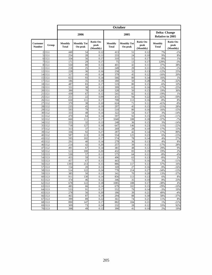
205

CustomerNumber Group Monthly

TotalMonthly Tot

On-peak

Ratio On-peak

(Monthly)

Monthly Total

Monthly Tot On-peak

Ratio On-peak

(Monthly)

Monthly Total

Ratio On-peak

(Monthly)2 CG1 440 54 0.12 413 51 0.12 7% -1%5 CG1 254 28 0.11 233 24 0.10 9% 8%6 CG1 334 56 0.17 310 51 0.17 8% 1%7 CG1 171 29 0.17 75 13 0.17 129% -3%8 CG1 550 80 0.15 401 42 0.11 37% 38%

11 CG1 218 25 0.11 249 29 0.11 -12% -1%12 CG1 228 36 0.16 258 32 0.13 -12% 25%14 CG1 317 45 0.14 379 45 0.12 -16% 20%15 CG1 655 93 0.14 566 80 0.14 16% 1%17 CG1 186 35 0.19 180 50 0.28 3% -32%18 CG1 487 83 0.17 519 80 0.15 -6% 10%19 CG1 331 38 0.12 399 62 0.16 -17% -25%20 CG1 390 78 0.20 328 50 0.15 19% 30%21 CG1 439 67 0.15 541 82 0.15 -19% 1%25 CG1 251 22 0.09 431 94 0.22 -42% -59%26 CG1 650 111 0.17 708 113 0.16 -8% 8%27 CG2 370 38 0.10 624 71 0.11 -41% -8%28 CG2 235 45 0.19 297 45 0.15 -21% 28%29 CG2 593 79 0.13 510 80 0.16 16% -15%30 CG2 333 48 0.14 322 54 0.17 3% -14%31 CG2 470 64 0.14 597 92 0.15 -21% -11%32 CG2 660 111 0.17 1040 188 0.18 -37% -7%34 CG2 255 32 0.13 248 36 0.15 3% -14%35 CG2 718 127 0.18 647 146 0.23 11% -22%37 CG2 313 37 0.12 269 28 0.10 17% 13%39 CG2 336 92 0.27 287 42 0.14 17% 89%40 CG2 587 113 0.19 554 125 0.23 6% -15%43 CG2 595 102 0.17 574 78 0.14 4% 27%45 CG2 291 40 0.14 279 36 0.13 4% 8%46 CG2 214 42 0.20 257 39 0.15 -17% 28%47 CG2 491 67 0.14 381 48 0.12 29% 9%50 CG2 513 100 0.20 432 83 0.19 19% 2%53 CG3 530 57 0.11 575 64 0.11 -8% -4%54 CG3 455 59 0.13 496 63 0.13 -8% 2%55 CG3 457 67 0.15 443 73 0.16 3% -11%56 CG3 1393 213 0.15 886 117 0.13 57% 16%57 CG3 154 20 0.13 169 27 0.16 -9% -16%58 CG3 514 122 0.24 778 214 0.27 -34% -13%59 CG3 385 50 0.13 341 70 0.20 13% -37%60 CG3 911 130 0.14 856 113 0.13 6% 8%61 CG3 374 46 0.12 346 35 0.10 8% 23%62 CG3 678 122 0.18 1085 188 0.17 -38% 4%63 CG3 485 66 0.14 679 102 0.15 -29% -10%64 CG3 533 91 0.17 552 79 0.14 -3% 19%65 CG3 278 56 0.20 186 39 0.21 49% -4%66 CG3 465 87 0.19 294 88 0.30 58% -37%67 CG3 399 89 0.22 361 74 0.21 11% 8%68 CG3 890 147 0.17 882 184 0.21 1% -21%69 CG3 309 73 0.24 232 28 0.12 33% 92%70 CG3 398 49 0.12 390 41 0.10 2% 19%

October

2006 2005 Delta: Change Relative to 2005

206

CustomerNumber Group Monthly

TotalMonthly Tot

On-peak

Ratio On-peak

(Monthly)

Monthly Total

Monthly Tot On-peak

Ratio On-peak

(Monthly)

Monthly Total

Ratio On-peak

(Monthly)71 CG3 908 224 0.25 760 228 0.30 20% -18%72 CG3 444 40 0.09 416 36 0.09 7% 5%73 CG3 752 94 0.13 776 95 0.12 -3% 3%74 CG3 679 131 0.19 783 159 0.20 -13% -5%75 CG3 316 59 0.19 338 80 0.24 -7% -21%76 CG3 339 43 0.13 282 40 0.14 20% -12%77 CG3 265 59 0.22 257 59 0.23 3% -3%78 CG3 837 150 0.18 872 165 0.19 -4% -5%79 CG3 301 55 0.18 408 77 0.19 -26% -3%80 CG3 512 167 0.33 507 104 0.20 1% 60%81 CG3 805 180 0.22 823 191 0.23 -2% -4%82 CG3 569 75 0.13 404 57 0.14 41% -7%83 CG3 421 49 0.12 353 42 0.12 19% -3%84 CG3 647 124 0.19 530 97 0.18 22% 5%85 CG3 320 40 0.13 228 24 0.10 41% 22%86 CG3 533 84 0.16 340 68 0.20 57% -21%87 CG3 372 26 0.07 365 34 0.09 2% -24%88 CG3 386 48 0.12 276 27 0.10 40% 28%89 CG3 404 57 0.14 445 69 0.16 -9% -9%90 CG3 929 138 0.15 599 81 0.13 55% 10%91 CG3 519 85 0.16 505 91 0.18 3% -9%92 CG3 687 135 0.20 640 85 0.13 7% 48%93 CG3 353 52 0.15 211 21 0.10 67% 52%94 CG3 324 45 0.14 337 50 0.15 -4% -6%95 CG3 478 76 0.16 537 91 0.17 -11% -6%96 CG3 485 56 0.12 533 56 0.10 -9% 11%97 CG3 799 121 0.15 931 170 0.18 -14% -17%98 TG1 707 112 0.16 651 101 0.16 9% 2%

100 TG1 564 101 0.18 558 95 0.17 1% 4%101 TG1 737 102 0.14 721 120 0.17 2% -17%104 TG1 791 125 0.16 460 65 0.14 72% 12%105 TG1 955 160 0.17 854 142 0.17 12% 1%106 TG1 599 98 0.16 516 63 0.12 16% 35%107 TG1 368 56 0.15 285 56 0.20 29% -22%108 TG1 94 13 0.14 145 21 0.14 -35% -4%111 TG1 1215 198 0.16 1266 184 0.15 -4% 12%112 TG1 262 23 0.09 172 20 0.11 52% -22%113 TG1 755 153 0.20 768 155 0.20 -2% 1%114 TG1 829 87 0.10 1092 162 0.15 -24% -30%115 TG1 234 27 0.11 369 53 0.14 -37% -20%119 TG1 394 55 0.14 353 50 0.14 12% -2%120 TG1 650 111 0.17 628 102 0.16 3% 5%122 TG1 829 129 0.16 679 52 0.08 22% 103%125 TG2 692 101 0.15 672 170 0.25 3% -42%127 TG2 581 106 0.18 481 78 0.16 21% 13%129 TG2 614 113 0.18 570 100 0.18 8% 5%130 TG2 406 70 0.17 279 65 0.23 46% -26%

October, cont'd

2006 2005 Delta: Change Relative to 2005

207

CustomerNumber Group Monthly

TotalMonthly Tot

On-peak

Ratio On-peak

(Monthly)

Monthly Total

Monthly Tot On-peak

Ratio On-peak

(Monthly)

Monthly Total

Ratio On-peak

(Monthly)131 TG2 407 59 0.15 401 62 0.15 2% -6%133 TG2 485 84 0.17 381 53 0.14 27% 24%134 TG2 405 70 0.17 403 77 0.19 0% -10%136 TG2 428 54 0.13 422 67 0.16 1% -21%137 TG2 1200 201 0.17 758 182 0.24 58% -30%138 TG2 572 87 0.15 525 105 0.20 9% -23%139 TG2 946 171 0.18 799 145 0.18 18% 0%141 TG2 600 100 0.17 620 139 0.22 -3% -25%142 TG2 382 50 0.13 376 72 0.19 2% -32%143 TG2 673 138 0.20 444 86 0.19 52% 5%145 TG2 528 84 0.16 435 55 0.13 21% 25%147 TG2 771 132 0.17 735 113 0.15 5% 12%150 TG3 153 20 0.13 189 33 0.18 -19% -25%152 TG3 556 153 0.28 633 114 0.18 -12% 54%153 TG3 635 67 0.11 632 87 0.14 0% -22%154 TG3 477 68 0.14 611 134 0.22 -22% -35%155 TG3 247 19 0.08 286 28 0.10 -14% -19%156 TG3 479 72 0.15 446 81 0.18 7% -18%157 TG3 426 49 0.11 512 78 0.15 -17% -25%158 TG3 250 57 0.23 232 34 0.15 8% 55%163 TG3 934 114 0.12 972 182 0.19 -4% -35%164 TG3 315 45 0.14 601 128 0.21 -48% -33%165 TG3 710 129 0.18 564 128 0.23 26% -20%167 TG3 581 81 0.14 691 105 0.15 -16% -9%170 TG3 188 25 0.13 178 37 0.21 5% -35%171 TG3 638 152 0.24 626 110 0.18 2% 36%173 TG3 423 73 0.17 401 64 0.16 6% 8%176 TG4 265 21 0.08 194 22 0.12 36% -31%179 TG4 392 53 0.14 387 48 0.12 1% 9%181 TG4 791 107 0.14 1292 229 0.18 -39% -24%182 TG4 290 37 0.13 249 41 0.16 17% -23%183 TG4 537 63 0.12 447 53 0.12 20% -1%184 TG4 276 25 0.09 282 31 0.11 -2% -20%185 TG4 327 59 0.18 337 53 0.16 -3% 15%188 TG4 343 36 0.11 397 48 0.12 -14% -11%189 TG4 299 39 0.13 287 30 0.10 4% 26%191 TG4 376 54 0.14 618 109 0.18 -39% -18%193 TG4 661 103 0.16 533 101 0.19 24% -18%194 TG4 409 69 0.17 437 83 0.19 -6% -12%195 TG4 826 117 0.14 549 96 0.18 51% -19%196 TG4 537 85 0.16 425 56 0.13 26% 20%197 TG4 474 96 0.20 459 118 0.26 3% -21%199 TG4 1281 234 0.18 962 155 0.16 33% 14%201 TG4 507 72 0.14 388 72 0.19 31% -24%

October, cont'd

2006 2005 Delta: Change Relative to 2005

208

CustomerNumber Group Monthly

TotalMonthly Tot

On-peak

Ratio On-peak

(Monthly)

Monthly Total

Monthly Tot On-peak

Ratio On-peak

(Monthly)

Monthly Total

Ratio On-peak

(Monthly)2 CG1 536 79 0.15 617 102 0.16 -13% -9%5 CG1 361 48 0.12 365 62 0.16 -1% -21%6 CG1 387 66 0.17 309 64 0.20 25% -15%7 CG1 135 22 0.16 76 13 0.17 78% -1%8 CG1 712 110 0.15 476 65 0.13 50% 17%

11 CG1 264 24 0.09 242 21 0.09 9% 8%12 CG1 292 45 0.15 344 51 0.14 -15% 7%14 CG1 314 52 0.17 355 40 0.11 -11% 51%15 CG1 679 82 0.12 831 124 0.15 -18% -16%17 CG1 204 38 0.19 192 49 0.26 6% -27%18 CG1 581 95 0.16 617 114 0.18 -6% -10%19 CG1 399 64 0.16 422 80 0.19 -5% -16%20 CG1 388 75 0.19 307 57 0.19 26% 4%21 CG1 538 96 0.18 568 101 0.18 -5% -1%25 CG1 404 85 0.18 617 166 0.26 -34% -30%26 CG1 891 117 0.14 849 106 0.13 5% 7%27 CG2 461 65 0.14 661 101 0.16 -30% -11%28 CG2 296 47 0.16 354 65 0.18 -16% -12%29 CG2 579 81 0.14 444 86 0.19 30% -28%30 CG2 307 38 0.12 358 58 0.16 -14% -23%31 CG2 578 78 0.13 680 102 0.15 -15% -10%32 CG2 718 127 0.18 1175 224 0.19 -39% -7%34 CG2 286 36 0.12 258 51 0.20 11% -36%35 CG2 925 188 0.20 767 195 0.25 21% -21%37 CG2 345 43 0.12 314 50 0.15 10% -22%39 CG2 422 87 0.22 375 44 0.12 13% 77%40 CG2 566 92 0.16 613 156 0.25 -8% -36%43 CG2 636 92 0.15 585 91 0.15 9% -5%45 CG2 293 42 0.14 361 85 0.22 -19% -35%46 CG2 285 43 0.16 310 51 0.16 -8% -4%47 CG2 518 62 0.12 417 52 0.12 24% -3%50 CG2 505 99 0.20 448 87 0.19 13% 1%53 CG3 707 109 0.14 771 112 0.14 -8% 2%54 CG3 511 71 0.14 550 88 0.16 -7% -12%55 CG3 452 71 0.16 559 92 0.16 -19% -4%56 CG3 1237 207 0.17 912 162 0.18 36% -6%57 CG3 191 29 0.15 208 36 0.17 -8% -16%58 CG3 875 231 0.26 938 257 0.27 -7% -4%59 CG3 478 71 0.15 480 111 0.22 -1% -35%60 CG3 930 120 0.13 1013 157 0.15 -8% -14%61 CG3 410 49 0.12 405 38 0.09 1% 25%62 CG3 676 106 0.16 1060 205 0.19 -36% -19%63 CG3 568 79 0.14 705 96 0.14 -19% 1%64 CG3 577 88 0.16 648 89 0.14 -11% 14%65 CG3 304 61 0.20 283 72 0.25 7% -20%66 CG3 551 115 0.20 469 127 0.28 18% -27%67 CG3 327 68 0.21 335 77 0.23 -2% -9%68 CG3 883 140 0.16 871 168 0.19 1% -18%69 CG3 291 67 0.23 201 22 0.11 45% 115%70 CG3 505 84 0.16 588 114 0.18 -14% -14%

Three-month Average (Aug - Oct)

2006 2005 Delta: Change Relative to 2005

209

CustomerNumber Group Monthly

TotalMonthly Tot

On-peak

Ratio On-peak

(Monthly)

Monthly Total

Monthly Tot On-peak

Ratio On-peak

(Monthly)

Monthly Total

Ratio On-peak

(Monthly)71 CG3 982 255 0.26 836 235 0.28 17% -8%72 CG3 511 44 0.09 500 23 0.05 2% 76%73 CG3 879 107 0.12 842 92 0.11 4% 11%74 CG3 769 165 0.21 753 168 0.22 2% -4%75 CG3 275 55 0.20 335 73 0.22 -18% -8%76 CG3 368 51 0.14 362 63 0.16 2% -14%77 CG3 298 68 0.23 278 64 0.23 7% 0%78 CG3 897 153 0.17 731 128 0.17 23% 0%79 CG3 340 58 0.17 515 117 0.22 -34% -23%80 CG3 576 187 0.32 661 131 0.20 -13% 62%81 CG3 766 167 0.22 831 198 0.24 -8% -9%82 CG3 659 94 0.14 541 91 0.16 22% -12%83 CG3 555 93 0.16 486 103 0.19 14% -18%84 CG3 765 163 0.21 684 141 0.20 12% 1%85 CG3 298 38 0.13 202 30 0.15 47% -15%86 CG3 590 102 0.17 478 96 0.20 23% -14%87 CG3 511 51 0.10 516 46 0.09 -1% 9%88 CG3 438 64 0.14 349 52 0.14 25% 3%89 CG3 476 67 0.14 490 82 0.17 -3% -17%90 CG3 965 157 0.16 799 139 0.17 21% -3%91 CG3 622 120 0.19 637 159 0.24 -2% -22%92 CG3 706 127 0.18 629 87 0.14 12% 32%93 CG3 353 58 0.16 275 40 0.14 28% 17%94 CG3 470 94 0.19 450 92 0.20 4% -5%95 CG3 661 107 0.16 635 126 0.20 4% -18%96 CG3 629 69 0.11 534 58 0.11 18% 3%97 CG3 937 139 0.15 983 164 0.17 -5% -11%98 TG1 890 120 0.14 781 107 0.14 14% -2%

100 TG1 818 163 0.20 586 113 0.19 40% 3%101 TG1 757 105 0.14 690 111 0.16 10% -13%104 TG1 940 158 0.17 592 101 0.17 59% 0%105 TG1 987 167 0.17 820 149 0.18 20% -6%106 TG1 581 96 0.16 414 78 0.19 40% -13%107 TG1 400 59 0.15 341 70 0.20 17% -26%108 TG1 115 16 0.14 151 21 0.14 -24% -1%111 TG1 1166 156 0.13 1144 158 0.14 2% -3%112 TG1 267 18 0.07 229 12 0.06 17% 13%113 TG1 867 179 0.20 811 169 0.21 7% -4%114 TG1 1085 86 0.08 1174 197 0.17 -8% -49%115 TG1 378 51 0.13 462 61 0.13 -18% -1%119 TG1 528 101 0.18 435 79 0.18 21% 1%120 TG1 624 105 0.17 749 154 0.20 -17% -17%122 TG1 888 110 0.12 535 30 0.05 66% 131%125 TG2 760 114 0.15 761 178 0.24 0% -37%127 TG2 568 100 0.18 620 113 0.18 -8% -3%129 TG2 582 100 0.17 567 109 0.19 3% -8%130 TG2 488 79 0.16 317 71 0.22 54% -29%

Three-month Average (Aug - Oct) -- cont'd

2006 2005 Delta: Change Relative to 2005

210

CustomerNumber Group Monthly

TotalMonthly Tot

On-peak

Ratio On-peak

(Monthly)

Monthly Total

Monthly Tot On-peak

Ratio On-peak

(Monthly)

Monthly Total

Ratio On-peak

(Monthly)131 TG2 436 54 0.12 510 88 0.17 -14% -24%133 TG2 454 79 0.18 312 48 0.16 46% 12%134 TG2 461 74 0.16 461 91 0.20 0% -17%136 TG2 474 82 0.17 450 84 0.18 5% -8%137 TG2 1157 238 0.21 865 228 0.26 34% -21%138 TG2 599 100 0.17 596 137 0.23 0% -26%139 TG2 1109 213 0.19 898 180 0.20 23% -4%141 TG2 621 94 0.15 692 116 0.17 -10% -11%142 TG2 392 52 0.13 431 82 0.19 -9% -31%143 TG2 702 133 0.19 680 119 0.18 3% 7%145 TG2 681 106 0.16 469 75 0.15 45% 4%147 TG2 841 186 0.22 777 140 0.18 8% 22%150 TG3 200 28 0.14 205 36 0.17 -2% -22%152 TG3 556 141 0.25 670 128 0.19 -17% 33%153 TG3 779 106 0.13 729 134 0.18 7% -29%154 TG3 547 73 0.13 700 175 0.25 -22% -46%155 TG3 213 25 0.12 271 31 0.11 -21% 11%156 TG3 549 90 0.16 496 113 0.23 11% -29%157 TG3 470 62 0.13 489 63 0.13 -4% 2%158 TG3 306 46 0.16 378 82 0.20 -19% -23%163 TG3 1326 172 0.13 1066 191 0.18 24% -29%164 TG3 675 118 0.17 805 173 0.22 -16% -23%165 TG3 933 177 0.19 554 115 0.20 68% -8%167 TG3 719 94 0.13 781 126 0.16 -8% -19%170 TG3 367 69 0.18 360 82 0.22 2% -21%171 TG3 730 145 0.20 837 179 0.21 -13% -4%173 TG3 479 77 0.16 442 73 0.16 8% -2%176 TG4 294 22 0.07 288 39 0.13 2% -44%179 TG4 520 65 0.12 592 97 0.16 -12% -24%181 TG4 1244 133 0.11 1367 225 0.16 -9% -32%182 TG4 292 39 0.13 259 34 0.13 13% 2%183 TG4 538 67 0.13 501 50 0.10 7% 25%184 TG4 272 29 0.10 281 30 0.11 -3% -2%185 TG4 386 55 0.15 498 70 0.15 -23% 1%188 TG4 544 89 0.15 459 73 0.15 19% 1%189 TG4 340 34 0.10 352 35 0.10 -4% 3%191 TG4 555 95 0.17 671 135 0.20 -17% -17%193 TG4 694 118 0.17 543 120 0.22 28% -23%194 TG4 467 80 0.17 453 82 0.18 3% -6%195 TG4 789 122 0.16 482 115 0.24 64% -35%196 TG4 694 109 0.15 492 71 0.14 41% 9%197 TG4 534 113 0.21 645 156 0.25 -17% -15%199 TG4 1493 246 0.17 1169 185 0.16 28% 5%201 TG4 515 62 0.12 420 71 0.17 23% -29%

Three-month Average (Aug - Oct) -- cont'd

2006 2005 Delta: Change Relative to 2005

Appendix IX Normality Results

211

212

Normality Testing Results for Dependent Variables, Treatment and Control Group #3 Only

Shapiro-Wilk Dependent Variable Statistic df Sig.*

AugTotDelta 0.946 109 0.000 AugPeakRationDelta 0.804 109 0.000 SeptTotDelta 0.874 109 0.000 SeptPeakRatioDelta 0.786 109 0.000 OctTotDelta 0.966 109 0.007 OctPeakRatioDelta 0.898 109 0.000 ThreeMonthTotDelta 0.952 109 0.001 ThreeMonthPeakRatioDelta 0.776 109 0.000 ShiftAugTotDelta 0.946 109 0.000 ShiftAugPeakRationDelta 0.804 109 0.000 ShiftSeptTotDelta 0.874 109 0.000 ShiftSeptPeakRatioDelta 0.786 109 0.000 ShiftOctTotDelta 0.966 109 0.007 ShiftOctPeakRatioDelta 0.898 109 0.000 ShiftThreeMonthTotDelta 0.952 109 0.001 ShiftThreeMonthPeakRatioDelta 0.776 109 0.000 LogShiftAugTotDelta 0.982 109 0.157 LogShiftAugPeakRationDelta 0.843 109 0.000 LogShiftSeptTotDelta 0.976 109 0.043 LogShiftSeptPeakRatioDelta 0.980 109 0.104 LogShiftOctTotDelta 0.959 109 0.002 LogShiftOctPeakRatioDelta 0.984 109 0.238 LogShiftThreeMonthTotDelta 0.989 109 0.483 LogShiftThreeMonthPeakRatioDelta 0.944 109 0.000 SqRtShiftAugTotDelta 0.974 109 0.030 SqRtShiftAugPeakRationDelta 0.906 109 0.000 SqRtShiftSeptTotDelta 0.940 109 0.000 SqRtShiftSeptPeakRatioDelta 0.914 109 0.000 SqRtShiftOctTotDelta 0.975 109 0.036 SqRtShiftOctPeakRatioDelta 0.953 109 0.001 SqRtShiftThreeMonthTotDelta 0.976 109 0.049 SqRtShiftThreeMonthPeakRatioDelta 0.881 109 0.000

* The null hypothesis that the data is normal is not rejected if the significance is greater than 0.05 (i.e. for normality, the significance level must be greater than 0.05).

213

Normality Testing Results for Dependent Variables, Treatment and Control Groups #1 & 2 Only Shapiro-Wilk Dependent Variable

Statistic df Sig.* AugTotDelta 0.957 96 0.003 AugPeakRationDelta 0.858 96 0.000 SeptTotDelta 0.881 96 0.000 SeptPeakRatioDelta 0.826 96 0.000 OctTotDelta 0.926 96 0.000 OctPeakRatioDelta 0.923 96 0.000 ThreeMonthTotDelta 0.947 96 0.001 ThreeMonthPeakRatioDelta 0.811 96 0.000 ShiftAugTotDelta 0.957 96 0.003 ShiftAugPeakRationDelta 0.858 96 0.000 ShiftSeptTotDelta 0.881 96 0.000 ShiftSeptPeakRatioDelta 0.826 96 0.000 ShiftOctTotDelta 0.926 96 0.000 ShiftOctPeakRatioDelta 0.923 96 0.000 ShiftThreeMonthTotDelta 0.947 96 0.001 ShiftThreeMonthPeakRatioDelta 0.811 96 0.000 LogShiftAugTotDelta 0.990 96 0.691 LogShiftAugPeakRationDelta 0.826 96 0.000 LogShiftSeptTotDelta 0.975 96 0.061 LogShiftSeptPeakRatioDelta 0.979 96 0.124 LogShiftOctTotDelta 0.953 96 0.002 LogShiftOctPeakRatioDelta 0.974 96 0.050 LogShiftThreeMonthTotDelta 0.990 96 0.661 LogShiftThreeMonthPeakRatioDelta 0.961 96 0.006 SqRtShiftAugTotDelta 0.983 96 0.271 SqRtShiftAugPeakRationDelta 0.931 96 0.000 SqRtShiftSeptTotDelta 0.946 96 0.001 SqRtShiftSeptPeakRatioDelta 0.935 96 0.000 SqRtShiftOctTotDelta 0.962 96 0.006 SqRtShiftOctPeakRatioDelta 0.969 96 0.022 SqRtShiftThreeMonthTotDelta 0.975 96 0.066 SqRtShiftThreeMonthPeakRatioDelta 0.910 96 0.000

* The null hypothesis that the data is normal is not rejected if the significance is greater than 0.05 (i.e. for normality, the significance level must be greater than 0.05).

214

Normality Testing Results for Dependent Variables, Treatment and All Control Groups Shapiro-Wilk Dependent Variable

Statistic df Sig.* AugTotDelta 0.957 141 0.000 AugPeakRationDelta 0.809 141 0.000 SeptTotDelta 0.895 141 0.000 SeptPeakRatioDelta 0.792 141 0.000 OctTotDelta 0.945 141 0.000 OctPeakRatioDelta 0.921 141 0.000 ThreeMonthTotDelta 0.957 141 0.000 ThreeMonthPeakRatioDelta 0.792 141 0.000 ShiftAugTotDelta 0.957 141 0.000 ShiftAugPeakRationDelta 0.809 141 0.000 ShiftSeptTotDelta 0.895 141 0.000 ShiftSeptPeakRatioDelta 0.792 141 0.000 ShiftOctTotDelta 0.945 141 0.000 ShiftOctPeakRatioDelta 0.921 141 0.000 ShiftThreeMonthTotDelta 0.957 141 0.000 ShiftThreeMonthPeakRatioDelta 0.792 141 0.000 LogShiftAugTotDelta 0.989 141 0.325 LogShiftAugPeakRationDelta 0.860 141 0.000 LogShiftSeptTotDelta 0.978 141 0.025 LogShiftSeptPeakRatioDelta 0.980 141 0.035 LogShiftOctTotDelta 0.968 141 0.002 LogShiftOctPeakRatioDelta 0.979 141 0.029 LogShiftThreeMonthTotDelta 0.991 141 0.548 LogShiftThreeMonthPeakRatioDelta 0.951 141 0.000 SqRtShiftAugTotDelta 0.983 141 0.081 SqRtShiftAugPeakRationDelta 0.912 141 0.000 SqRtShiftSeptTotDelta 0.956 141 0.000 SqRtShiftSeptPeakRatioDelta 0.915 141 0.000 SqRtShiftOctTotDelta 0.974 141 0.009 SqRtShiftOctPeakRatioDelta 0.969 141 0.003 SqRtShiftThreeMonthTotDelta 0.982 141 0.058 SqRtShiftThreeMonthPeakRatioDelta 0.891 141 0.000

* The null hypothesis that the data is normal is not rejected if the significance is greater than 0.05 (i.e. for normality, the significance level must be greater than 0.05).

215

Normality Testing Results for Dependent Variables, Treatment Groups Only Shapiro-Wilk Dependent Variable

Statistic df Sig.* AugTotDelta 0.941 64 0.004 AugPeakRatioDelta 0.849 64 0.000 SeptTotDelta 0.837 64 0.000 SeptPeakRatioDelta 0.830 64 0.000 OctTotDelta 0.974 64 0.193 OctPeakRatioDelta 0.879 64 0.000 ThreeMonthAveTotDelta 0.928 64 0.001 ThreeMonthAvePeakRatioDelta 0.779 64 0.000 ShiftAugTotDelta 0.941 64 0.004 ShiftAugPeakRationDelta 0.849 64 0.000 ShiftSeptTotDelta 0.837 64 0.000 ShiftSeptPeakRatioDelta 0.830 64 0.000 ShiftOctTotDelta 0.974 64 0.193 ShiftOctPeakRatioDelta 0.879 64 0.000 ShiftThreeMonthTotDelta 0.928 64 0.001 ShiftThreeMonthPeakRatioDelta 0.779 64 0.000 LogShiftAugTotDelta 0.979 64 0.361 LogShiftAugPeakRationDelta 0.806 64 0.000 LogShiftSeptTotDelta 0.952 64 0.015 LogShiftSeptPeakRatioDelta 0.974 64 0.204 LogShiftOctTotDelta 0.940 64 0.004 LogShiftOctPeakRatioDelta 0.970 64 0.116 LogShiftThreeMonthTotDelta 0.968 64 0.096 LogShiftThreeMonthPeakRatioDelta 0.946 64 0.008 SqRtShiftAugTotDelta 0.969 64 0.102 SqRtShiftAugPeakRationDelta 0.925 64 0.001 SqRtShiftSeptTotDelta 0.904 64 0.000 SqRtShiftSeptPeakRatioDelta 0.941 64 0.004 SqRtShiftOctTotDelta 0.970 64 0.126 SqRtShiftOctPeakRatioDelta 0.936 64 0.002 SqRtShiftThreeMonthTotDelta 0.952 64 0.014 SqRtShiftThreeMonthPeakRatioDelta 0.893 64 0.000 AugTotDelta 0.941 64 0.004

* The null hypothesis that the data is normal is not rejected if the significance is greater than 0.05 (i.e. for normality, the significance level must be greater than 0.05).

Appendix X Mann-Whitney Results for Treatment and Control Groups

216

217

Mann-Whitney Significance Results for Consumption Changes Comparing All Feedback Recipients and All Non-Recipients

Dependent Variable Mann-

Whitney Statistic

Sig (2-tailed)*

Medians for Feedback and Non-Feedback Groups (Listed for Significant Findings Only)

AugTotDelta 2397 0.781

AugPeakRatioDelta 2292 0.476

SeptTotDelta 1964 0.038 Feedback Median = 0.08; No Feedback Median = -0.02

SeptPeakRatioDelta 2446 0.941

OctTotDelta 2321 0.554

OctPeakRatioDelta 1860 0.012 Feedback Median = -0.12; No Feedback Median = -0.01

ThreeMonthAveTotDelta 2228 0.328

ThreeMonthAvePeakRatioDelta 2233 0.339

Subdividing into “High” and “Low” Consumer Groups

AugTotDelta – High Consumers 607 0.880

AugTotDelta – Low Consumers 569 0.625

AugPeakRatioDelta – High Consumers 565 0.524

AugPeakRatioDelta – Low Consumers 579 0.711

SeptTotDelta – High Consumers 494 0.133

SeptTotDelta – Low Consumers 484 0.144

SeptPeakRatioDelta – High Consumers 483 0.103

SeptPeakRatioDelta – Low Consumers 504 0.220

OctTotDelta – High Consumers 458 0.049 Feedback Median = 0.03; No Feedback Median = -0.04

OctTotDelta – Low Consumers 505 0.362

OctPeakRatioDelta – High Consumers 490 0.110

OctPeakRatioDelta – Low Consumers 422 0.056

ThreeMonthAveTotDelta – High Consumers 479 0.084

ThreeMonthAveTotDelta – Low Consumers 585 0.818

ThreeMonthAvePeakRatioDelta – High Consumers 550 0.363

ThreeMonthAvePeakRatioDelta – Low Consumers 590 0.864

218

Mann-Whitney Test Results For Consumption Changes Comparing Feedback Recipients and CG1/CG2 Non-Recipients – Significant Results Only

Dependent Variable Mann-

Whitney Statistic

Sig (2-tailed)*

Medians for Feedback and Non-Feedback Groups (Listed for Significant Findings Only)

AugTotDelta 1013 0.932

AugPeakRatioDelta 936 0.494

SeptTotDelta 733 0.024 Feedback Median = 0.075; No Feedback Median = -0.06

SeptPeakRatioDelta 977 0.715

OctTotDelta 899 0.331

OctPeakRatioDelta 743 0.029 Feedback Median = -0.115; No Feedback Median = 0.01

ThreeMonthAveTotDelta 884 0.277

ThreeMonthAvePeakRatioDelta 1014 0.938

Subdividing into “High” and “Low” Consumer Groups

AugTotDelta – High Consumers 186 0.475

AugTotDelta – Low Consumers 253 0.572

AugPeakRatioDelta – High Consumers 210 0.886

AugPeakRatioDelta – Low Consumers 255 0.601

SeptTotDelta – High Consumers 107 0.009 Feedback Median = 0.005; No Feedback Median = -0.16

SeptTotDelta – Low Consumers 209 0.138

SeptPeakRatioDelta – High Consumers 204 0.775

SeptPeakRatioDelta – Low Consumers 245 0.464

OctTotDelta – High Consumers 144 0.144

OctTotDelta – Low Consumers 274 0.843

OctPeakRatioDelta – High Consumers 171 0.425

OctPeakRatioDelta - Low Consumers 184 0.039 Feedback Median = -0.12;

No Feedback Median = 0.08 ThreeMonthAveTotDelta – Low Consumers 272 0.867

ThreeMonthAveTotDelta – High Consumers 132 0.046 Feedback Median = 0.025;

No Feedback Median = -0.105 ThreeMonthAvePeakRatioDelta – Low Consumers 270 0.834

ThreeMonthAvePeakRatioDelta – High Consumers 205 0.793

219

Mann-Whitney Significance Results for Consumption Changes Comparing Feedback Recipients and Only CG3 Non-Recipients

Dependent Variable Mann-

Whitney Statistic

Sig (2-tailed)*

Medians for Feedback and Non-Feedback Groups (Listed for Significant Findings Only)

AugTotDelta 1362 0.631

AugPeakRatioDelta 1180 0.110

SeptTotDelta 1231 0.198

SeptPeakRatioDelta 1375 0.689

OctTotDelta 1422 0.912

OctPeakRatioDelta 1117 0.047 Feedback Median = -0.12; No Feedback Median = -0.04

ThreeMonthAveTotDelta 1344 0.555

ThreeMonthAvePeakRatioDelta 1219 0.174

Subdividing into “High” and “Low” Consumer Groups

AugTotDelta – High Consumers 350 0.673

AugTotDelta – Low Consumers 271 0.216

AugPeakRatioDelta – High Consumers 318 0.335

AugPeakRatioDelta – Low Consumers 274 0.237

SeptTotDelta – High Consumers 333 0.508

SeptTotDelta – Low Consumers 296 0.370

SeptPeakRatioDelta – High Consumers 297 0.203

SeptPeakRatioDelta – Low Consumers 319 0.626

OctTotDelta – High Consumers 291 0.216

OctTotDelta – Low Consumers 288 0.231

OctPeakRatioDelta – High Consumers 273 0.122

OctPeakRatioDelta – Low Consumers 289 0.238

ThreeMonthAveTotDelta – High Consumers 318 0.394

ThreeMonthAveTotDelta – Low Consumers 343 0.874

ThreeMonthAvePeakRatioDelta – High Consumers 259 0.063

ThreeMonthAvePeakRatioDelta – Low Consumers 334 0.751

Appendix XI Two-Way Univariate ANOVA Results

220

221

Tests of Between-Subjects Effects Dependent Variable: OctTotDelta

Source Type III Sum of Squares df Mean Square F Sig.

Corrected Model .436(a) 3 .145 2.720 .052 Intercept .286 1 .286 5.351 .024 HistVsComp .211 1 .211 3.954 .051 MailVsEmail .227 1 .227 4.242 .044 HistVsComp * MailVsEmail .015 1 .015 .275 .602

Error 3.204 60 .053 Total 3.946 64 Corrected Total 3.640 63

a R Squared = .120 (Adjusted R Squared = .076) Tests of Between-Subjects Effects Dependent Variable: LogShiftAugTotDelta

Source Type III Sum of Squares df Mean Square F Sig.

Corrected Model .043(a) 3 .014 .645 .589 Intercept .408 1 .408 18.211 .000 HistVsComp .022 1 .022 .991 .323 MailVsEmail .013 1 .013 .565 .455 HistVsComp * MailVsEmail .008 1 .008 .365 .548

Error 1.346 60 .022 Total 1.799 64 Corrected Total 1.389 63

a R Squared = .031 (Adjusted R Squared = -.017) Tests of Between-Subjects Effects Dependent Variable: LogShiftSeptPeakRatioDelta

Source Type III Sum of Squares df Mean Square F Sig.

Corrected Model .229(a) 3 .076 2.278 .089 Intercept 1.783 1 1.783 53.282 .000 HistVsComp .168 1 .168 5.018 .029 MailVsEmail .019 1 .019 .581 .449 HistVsComp * MailVsEmail .043 1 .043 1.274 .263

Error 2.008 60 .033 Total 4.017 64 Corrected Total 2.236 63

a R Squared = .102 (Adjusted R Squared = .057)

222

Tests of Between-Subjects Effects Dependent Variable: LogShiftOctPeakRatioDelta

Source Type III Sum of Squares df Mean Square F Sig.

Corrected Model .054(a) 3 .018 .991 .403 Intercept 1.407 1 1.407 76.808 .000 HistVsComp .020 1 .020 1.094 .300 MailVsEmail .007 1 .007 .378 .541 HistVsComp * MailVsEmail .028 1 .028 1.538 .220

Error 1.099 60 .018 Total 2.557 64 Corrected Total 1.153 63

a R Squared = .047 (Adjusted R Squared = .000) Tests of Between-Subjects Effects Dependent Variable: LogShiftThreeMonthTotDelta

Source Type III Sum of Squares df Mean Square F Sig.

Corrected Model .049(a) 3 .016 1.352 .266 Intercept .281 1 .281 23.166 .000 HistVsComp .034 1 .034 2.763 .102 MailVsEmail .004 1 .004 .300 .586 HistVsComp * MailVsEmail .014 1 .014 1.157 .286

Error .728 60 .012 Total 1.053 64 Corrected Total .777 63

a R Squared = .063 (Adjusted R Squared = .016) Tests of Between-Subjects Effects Dependent Variable: SqRtShiftAugTotDelta

Source Type III Sum of Squares df Mean Square F Sig.

Corrected Model .060(a) 3 .020 .790 .504 Intercept 54.682 1 54.682 2155.434 .000 HistVsComp .030 1 .030 1.201 .278 MailVsEmail .018 1 .018 .691 .409 HistVsComp * MailVsEmail .012 1 .012 .462 .499

Error 1.522 60 .025 Total 56.360 64 Corrected Total 1.582 63

a R Squared = .038 (Adjusted R Squared = -.010)

223

Tests of Between-Subjects Effects Dependent Variable: SqRtShiftOctTotDelta

Source Type III Sum of Squares df Mean Square F Sig.

Corrected Model .131(a) 3 .044 2.712 .053 Intercept 54.278 1 54.278 3365.184 .000 MailVsEmail .071 1 .071 4.373 .041 HistVsComp .063 1 .063 3.894 .053 MailVsEmail * HistVsComp .003 1 .003 .169 .682

Error .968 60 .016 Total 55.630 64 Corrected Total 1.099 63

a R Squared = .119 (Adjusted R Squared = .075)

Appendix XII Kruskal-Wallis Results

224

225

Main Effect Tests Test Statistics(a,b) AugTotDelta Chi-Square .987 df 1 Asymp. Sig. .320

a Kruskal Wallis Test b Grouping Variable: HistVsComp

AugTotDelta Chi-Square 1.029 df 1 Asymp. Sig. .310

a Kruskal Wallis Test b Grouping Variable: MailVsEmail Test Statistics(a,b)

AugPeakRatio

Delta Chi-Square .022 df 1 Asymp. Sig. .883

a Kruskal Wallis Test b Grouping Variable: HistVsComp

AugPeakRatio

Delta Chi-Square .127 df 1 Asymp. Sig. .722

a Kruskal Wallis Test b Grouping Variable: MailVsEmail

226

Test Statistics(a,b) SeptTotDelta Chi-Square 1.154 df 1 Asymp. Sig. .283

a Kruskal Wallis Test b Grouping Variable: HistVsComp SeptTotDelta Chi-Square .822 df 1 Asymp. Sig. .365

a Kruskal Wallis Test b Grouping Variable: MailVsEmail Test Statistics(a,b)

SeptPeakRatio

Delta Chi-Square 3.189 df 1 Asymp. Sig. .074

a Kruskal Wallis Test b Grouping Variable: HistVsComp

SeptPeakRatio

Delta Chi-Square .282 df 1 Asymp. Sig. .596

a Kruskal Wallis Test b Grouping Variable: MailVsEmail Test Statistics(a,b) OctTotDelta Chi-Square 3.237 df 1 Asymp. Sig. .072

a Kruskal Wallis Test b Grouping Variable: HistVsComp OctTotDelta Chi-Square 4.088 df 1 Asymp. Sig. .043

a Kruskal Wallis Test b Grouping Variable: MailVsEmail

227

Test Statistics(a,b)

OctPeakRatioD

elta Chi-Square .961 df 1 Asymp. Sig. .327

a Kruskal Wallis Test b Grouping Variable: HistVsComp

OctPeakRatioD

elta Chi-Square .055 df 1 Asymp. Sig. .814

a Kruskal Wallis Test b Grouping Variable: MailVsEmail Test Statistics(a,b)

ThreeMonthAv

eTotDelta Chi-Square 2.596 df 1 Asymp. Sig. .107

a Kruskal Wallis Test b Grouping Variable: HistVsComp

ThreeMonthAv

eTotDelta Chi-Square .240 df 1 Asymp. Sig. .624

a Kruskal Wallis Test b Grouping Variable: MailVsEmail

228

Test Statistics(a,b)

ThreeMonthAvePeakRatioDelt

a Chi-Square .858 df 1 Asymp. Sig. .354

a Kruskal Wallis Test b Grouping Variable: HistVsComp

ThreeMonthAvePeakRatioDelt

a Chi-Square .038 df 1 Asymp. Sig. .846

a Kruskal Wallis Test b Grouping Variable: MailVsEmail Interaction Effect Tests Test Statistics(a,b)

AugTotDelta

AugPeakRatioDelt

a SeptTot

Delta

SeptPeakRatioDelt

a OctTotDelta

OctPeakRatioDelt

a

ThreeMonthAveTo

tDelta

ThreeMonthAvePeakRatioD

elta Chi-Square .187 .292 .219 .187 .747 .130 .219 .032

df 1 1 1 1 1 1 1 1Asymp. Sig. .666 .589 .640 .666 .387 .719 .640 .857

a Kruskal Wallis Test b Grouping Variable: HistVsComp with MailVsEmail held at “Mail” Test Statistics(a,b)

AugTotDelta

AugPeakRatioDelt

a SeptTot

Delta

SeptPeakRatioDelt

a OctTotDelta

OctPeakRatioDelt

a

ThreeMonthAveTo

tDelta

ThreeMonthAvePeakRatioD

elta Chi-Square 1.225 .264 3.452 3.452 2.756 2.889 3.600 3.025

df 1 1 1 1 1 1 1 1Asymp. Sig. .268 .607 .063 .063 .097 .089 .058 .082

a Kruskal Wallis Test b Grouping Variable: HistVsComp with MailVsEmail held at “Email” For an interaction, the significances for each dependent variable at Mail and Email must add to less than 0.05.

229

Test Statistics(a,b)

AugTotDelta

AugPeakRatioDelt

a SeptTot

Delta

SeptPeakRatioDelt

a OctTotDelta

OctPeakRatioDelt

a

ThreeMonthAveTo

tDelta

ThreeMonthAvePeakRatioD

elta Chi-Square 1.365 .091 .460 1.278 .751 1.036 .411 1.455

df 1 1 1 1 1 1 1 1

Asymp. Sig. .243 .763 .498 .258 .386 .309 .522 .228

a Kruskal Wallis Test b Grouping Variable: MailVsEmail with HistVsComp held at “Hist” Test Statistics(a,b)

AugTotDelta

AugPeakRatioDelt

a SeptTot

Delta

SeptPeakRatioDelt

a OctTotDelta

OctPeakRatioDelt

a

ThreeMonthAveTo

tDelta

ThreeMonthAvePeakRatioD

elta Chi-Square .029 .788 4.715 .029 3.494 1.078 1.506 .437

df 1 1 1 1 1 1 1 1Asymp. Sig. .865 .375 .030 .865 .062 .299 .220 .509

a Kruskal Wallis Test b Grouping Variable: MailVsEmail with HistVsComp held at “Comp” For an interaction, the significances for each dependent variable at Hist and Comp must add to less than 0.05.

Appendix XIII Survey #2 Results Tables

230

231

Feedback

Frequency Percent Valid Percent Cumulative

Percent Yes 44 33.8 33.8 33.8No 86 66.2 66.2 100.0

Valid

Total 130 100.0 100.0 Type

Frequency Percent Valid Percent Cumulative

Percent Historic 24 18.5 18.5 18.5 Comparative 20 15.4 15.4 33.8 Non-PII - TOU 68 52.3 52.3 86.2 Non-PII - non-TOU 15 11.5 11.5 97.7 Invalid Feedback - Non-PII - TOU 3 2.3 2.3 100.0

Valid

Total 130 100.0 100.0 ActualMailOrEmail

Frequency Percent Valid Percent Cumulative

Percent 83 63.8 63.8 63.8Mail 27 20.8 20.8 84.6Email 20 15.4 15.4 100.0

Valid

Total 130 100.0 100.0 A1.SamePerson

Frequency Percent Valid Percent Cumulative

Percent Yes 126 96.9 96.9 96.9No 4 3.1 3.1 100.0

Valid

Total 130 100.0 100.0 A2.ChangesInSummer

Frequency Percent Valid Percent Cumulative

Percent Yes 33 25.4 25.4 25.4No 97 74.6 74.6 100.0

Valid

Total 130 100.0 100.0

232

A3.HomeDuringDay

Frequency Percent Valid Percent Cumulative

Percent Yes 73 56.2 56.2 56.2No 57 43.8 43.8 100.0

Valid

Total 130 100.0 100.0 A4.CFL

Frequency Percent Valid Percent Cumulative

Percent Yes, in most/all 59 45.4 45.7 45.7 Yes, one or two 38 29.2 29.5 75.2 No, but...in the next 2 years 19 14.6 14.7 89.9

No 12 9.2 9.3 99.2 I have not heard of CFLs 1 .8 .8 100.0

Valid

Total 129 99.2 100.0 Missing No response 1 .8 Total 130 100.0

VAR00012

Frequency Percent Valid Percent Cumulative

Percent 127 97.7 97.7 97.7 8 bulbs so far 1 .8 .8 98.5 garage, basement, outdoor lights 1 .8 .8 99.2

wrote "about one third" 1 .8 .8 100.0

Valid

Total 130 100.0 100.0 A5.KnowAveDailyConsumption

Frequency Percent Valid Percent Cumulative

Percent Yes 47 36.2 37.9 37.9 No 77 59.2 62.1 100.0

Valid

Total 124 95.4 100.0 Missing No response 6 4.6 Total 130 100.0

NonPartA6.WhatConsumesMost

233

Frequency Percent Valid Percent Cumulative

Percent 49 37.7 37.7 37.7 (answered but can't read the writing) 1 .8 .8 38.5

A.C. 1 .8 .8 39.2 A/C 13 10.0 10.0 49.2 A/C + dishwasher + washer/dryer 1 .8 .8 50.0

A/C or dryer 1 .8 .8 50.8 AC 1 .8 .8 51.5 AC and the clothes dryer 1 .8 .8 52.3 Air-Conditioner 1 .8 .8 53.1 Air con. 1 .8 .8 53.8 AIR CONDITION 1 .8 .8 54.6 air conditioner 11 8.5 8.5 63.1 Air conditioner 5 3.8 3.8 66.9 Air Conditioner 6 4.6 4.6 71.5 AIR CONDITIONER 6 4.6 4.6 76.2 Air conditioner or oven 1 .8 .8 76.9 air conditioning 2 1.5 1.5 78.5 Air Conditioning 2 1.5 1.5 80.0 AIR CONDITIONING 5 3.8 3.8 83.8 Air conditioning (central air) 1 .8 .8 84.6

air conditioning unit 1 .8 .8 85.4 appliances, ac in the summer, hot tub 1 .8 .8 86.2

central air 1 .8 .8 86.9 CENTRAL AIR 1 .8 .8 87.7 convection oven 1 .8 .8 88.5 dryer/spa/computer (servers) 1 .8 .8 89.2

Electric Stove 1 .8 .8 90.0 fans - table top & 2 floor ones 1 .8 .8 90.8

Fans 1 .8 .8 91.5 FRIDGE 1 .8 .8 92.3 Laundry Machine & dryer 1 .8 .8 93.1 less (?) 1 .8 .8 93.8 LIGHTING OR STOVE & FRIDGE (NO AC) 1 .8 .8 94.6

Refrigerator 1 .8 .8 95.4 REFRIGERATOR 1 .8 .8 96.2 REFRIGERATOR & AIR CON 1 .8 .8 96.9

Sprinkler System (Pump) 1 .8 .8 97.7

Valid

TV 1 .8 .8 98.5

234

Window A/C; Electric Appliances 1 .8 .8 99.2

yes 1 .8 .8 100.0

Total 130 100.0 100.0 A6.ESAppliance

Frequency Percent Valid Percent Cumulative

Percent 1 .8 8.3 8.3 Yes 11 8.5 91.7 100.0

Valid

Total 12 9.2 100.0 Missing No response 118 90.8 Total 130 100.0

A6.ESAC

Frequency Percent Valid Percent Cumulative

Percent 1 .8 16.7 16.7 Yes 5 3.8 83.3 100.0

Valid

Total 6 4.6 100.0 Missing No response 124 95.4 Total 130 100.0

A6.UpgradeFurnace

Frequency Percent Valid Percent Cumulative

Percent 1 .8 20.0 20.0 Yes 4 3.1 80.0 100.0

Valid

Total 5 3.8 100.0 Missing No response 125 96.2 Total 130 100.0

A6.UpgradeInsulation

Frequency Percent Valid Percent Cumulative

Percent 1 .8 16.7 16.7 Yes 5 3.8 83.3 100.0

Valid

Total 6 4.6 100.0 Missing No response 124 95.4 Total 130 100.0

A6.UpgradeWinDoors

235

Frequency Percent Valid Percent Cumulative

Percent 1 .8 12.5 12.5 Yes 7 5.4 87.5 100.0

Valid

Total 8 6.2 100.0 Missing No response 122 93.8 Total 130 100.0

A6.EnergyAudit

Frequency Percent Valid Percent Cumulative

Percent Valid Yes 13 10.0 100.0 100.0 Missing No response 117 90.0 Total 130 100.0

B1.HomeUseAwareness

Frequency Percent Valid Percent Cumulative

Percent Very high 21 16.2 16.2 16.2High 48 36.9 36.9 53.1Average 56 43.1 43.1 96.2Low 5 3.8 3.8 100.0

Valid

Total 130 100.0 100.0 B2.TalkConsChildren

Frequency Percent Valid Percent Cumulative

Percent Very frequently (every week) 15 11.5 12.8 12.8

Frequently (every month) 11 8.5 9.4 22.2 Occasionally (every few months) 11 8.5 9.4 31.6

Never 6 4.6 5.1 36.8 Not applicable 74 56.9 63.2 100.0

Valid

Total 117 90.0 100.0 Missing No response 13 10.0 Total 130 100.0

B2.TalkConsSpouse

Frequency Percent Valid Percent Cumulative

Percent

236

Very frequently (every week) 30 23.1 24.4 24.4

Frequently (every month) 40 30.8 32.5 56.9 Occasionally (every few months) 37 28.5 30.1 87.0

Never 3 2.3 2.4 89.4 Not applicable 13 10.0 10.6 100.0

Valid

Total 123 94.6 100.0 Missing No response 7 5.4 Total 130 100.0

B2.TalkConsOtherFam

Frequency Percent Valid Percent Cumulative

Percent Very frequently (every week) 6 4.6 4.9 4.9

Frequently (every month) 27 20.8 22.0 26.8 Occasionally (every few months) 45 34.6 36.6 63.4

Never 18 13.8 14.6 78.0 Not applicable 27 20.8 22.0 100.0

Valid

Total 123 94.6 100.0 Missing No response 7 5.4 Total 130 100.0

B2.TalkConsNeighbours

Frequency Percent Valid Percent Cumulative

Percent Very frequently (every week) 1 .8 .9 .9

Frequently (every month) 10 7.7 8.8 9.6 Occasionally (every few months) 42 32.3 36.8 46.5

Never 54 41.5 47.4 93.9 Not applicable 7 5.4 6.1 100.0

Valid

Total 114 87.7 100.0 Missing No response 16 12.3 Total 130 100.0

B2.TalkConsFriends

Frequency Percent Valid Percent Cumulative

Percent Valid Very frequently (every

week) 2 1.5 1.7 1.7

237

Frequently (every month) 12 9.2 10.2 11.9 Occasionally (every few months) 70 53.8 59.3 71.2

Never 28 21.5 23.7 94.9 Not applicable 6 4.6 5.1 100.0

Total 118 90.8 100.0 Missing No response 12 9.2 Total 130 100.0

B2.TalkConsCoWorkers

Frequency Percent Valid Percent Cumulative

Percent 1 .8 .9 .9 Very frequently (every week) 1 .8 .9 1.7

Frequently (every month) 8 6.2 7.0 8.7 Occasionally (every few months) 54 41.5 47.0 55.7

Never 37 28.5 32.2 87.8 Not applicable 14 10.8 12.2 100.0

Valid

Total 115 88.5 100.0 Missing No response 15 11.5 Total 130 100.0

B3.CommitmentConservation

Frequency Percent Valid Percent Cumulative

Percent Very committed 35 26.9 26.9 26.9 Committed 66 50.8 50.8 77.7 Somewhat committed 27 20.8 20.8 98.5 Minimally committed 2 1.5 1.5 100.0

Valid

Total 130 100.0 100.0 C1.HowOftenAdjustACDuringPeak

Frequency Percent Valid Percent Cumulative

Percent Always - programmable 50 38.5 39.1 39.1 Always - manual 28 21.5 21.9 60.9 Only during provincial appeals 4 3.1 3.1 64.1

Frequently (1 or 2 times per week) 9 6.9 7.0 71.1

Occasionally 15 11.5 11.7 82.8

Valid

Never 3 2.3 2.3 85.2

238

I don't know peak times 1 .8 .8 85.9 NA - no AC 3 2.3 2.3 88.3 Question not in this survey 15 11.5 11.7 100.0

Total 128 98.5 100.0 Missing 999 2 1.5 Total 130 100.0

C2.ReducePeakCommitment

Frequency Percent Valid Percent Cumulative

Percent Very committed 43 33.1 33.3 33.3 Committed 51 39.2 39.5 72.9 Somewhat committed 17 13.1 13.2 86.0 Minimally committed 3 2.3 2.3 88.4 Question not in this survey 15 11.5 11.6 100.0

Valid

Total 129 99.2 100.0 Missing No response 1 .8 Total 130 100.0

C3.MoreControlPatternsAndCosts

Frequency Percent Valid Percent Cumulative

Percent 1 .8 .8 .8 Yes 97 74.6 75.2 76.0 No 11 8.5 8.5 84.5 I didn't know about TOU pricing 5 3.8 3.9 88.4

Question not in this survey 15 11.5 11.6 100.0

Valid

Total 129 99.2 100.0 Missing No response 1 .8 Total 130 100.0

VAR00001

Frequency Percent Valid Percent Cumulative

Percent 129 99.2 99.2 99.2 (checked both "yes" and "no") 1 .8 .8 100.0

Valid

Total 130 100.0 100.0 C4.KnowPeakRate

239

Frequency Percent Valid Percent Cumulative

Percent Yes 71 54.6 55.5 55.5 No 42 32.3 32.8 88.3 Question not in this survey 15 11.5 11.7 100.0

Valid

Total 128 98.5 100.0 Missing No response 2 1.5 Total 130 100.0

C4.SpecifyRate

Frequency Percent Valid Percent Cumulative

Percent 47 36.2 36.2 36.2 (nothing written) 1 .8 .8 36.9 ~ 11.9 1 .8 .8 37.7 ~10 1 .8 .8 38.5 0.093 2 1.5 1.5 40.0 0.105 8 6.2 6.2 46.2 10 2 1.5 1.5 47.7 10.3 3 2.3 2.3 50.0 10.4 1 .8 .8 50.8 10.5 20 15.4 15.4 66.2 10.9 1 .8 .8 66.9 10+ 1 .8 .8 67.7 105 2 1.5 1.5 69.2 11.5 1 .8 .8 70.0 41-42 1 .8 .8 70.8 6-7 1 .8 .8 71.5 9 2 1.5 1.5 73.1 9 PLUS 1 .8 .8 73.8 9. 1 .8 .8 74.6 9.3 12 9.2 9.2 83.8 9.4 1 .8 .8 84.6 9.6 1 .8 .8 85.4 9.6 about 1 .8 .8 86.2 9.6? 1 .8 .8 86.9 9.8 1 .8 .8 87.7 9999 15 11.5 11.5 99.2 twice the edge (?) rate and three times the night rate

1 .8 .8 100.0

Valid

Total 130 100.0 100.0 C5.KnowPeakPeriod

240

Frequency Percent Valid Percent Cumulative

Percent Yes 82 63.1 65.1 65.1 No 29 22.3 23.0 88.1 Question not in this survey 15 11.5 11.9 100.0

Valid

Total 126 96.9 100.0 Missing No response 4 3.1 Total 130 100.0

C5.SpecifyPeriod

Frequency Percent Valid Percent Cumulative

Percent 31 23.8 23.8 23.8 (no response) 1 .8 .8 24.6 (nothing written) 1 .8 .8 25.4 10am, 2pm 1 .8 .8 26.2 10am, 7pm 1 .8 .8 26.9 10PM, 8AM (I think this is what he means) 1 .8 .8 27.7

11, 5 4 3.1 3.1 30.8 11,5 1 .8 .8 31.5 11am, 5or6pm 1 .8 .8 32.3 11am, 5pm 38 29.2 29.2 61.5 11am, 6pm 2 1.5 1.5 63.1 11am, 7pm 1 .8 .8 63.8 11am,5 1 .8 .8 64.6 12, 5 1 .8 .8 65.4 12md(?), 8pm 1 .8 .8 66.2 1pm, 6pm 1 .8 .8 66.9 5am, 11am 1 .8 .8 67.7 5pm, 10pm 1 .8 .8 68.5 6am, 11am 1 .8 .8 69.2 7-11am, 5-10pm 1 .8 .8 70.0 7&5 AM&PM, 11&8 AM&PM (??) 1 .8 .8 70.8

7, 10:30 1 .8 .8 71.5 7, 6 1 .8 .8 72.3 7am, 10pm 2 1.5 1.5 73.8 7am, 11am 1 .8 .8 74.6 7am, 11pm 1 .8 .8 75.4 7am, 5pm 2 1.5 1.5 76.9 7am, 6pm 2 1.5 1.5 78.5 7am, 7pm 1 .8 .8 79.2

Valid

8, 10 2 1.5 1.5 80.8

241

8, 6 I think (I think underlined) 1 .8 .8 81.5

8, 8 1 .8 .8 82.3 8am, 11pm 1 .8 .8 83.1 8am, 5pm 1 .8 .8 83.8 8am, 7pm 1 .8 .8 84.6 8am, 8pm 1 .8 .8 85.4 9999 15 11.5 11.5 96.9 9am, 5pm 1 .8 .8 97.7 9am, 8pm 1 .8 .8 98.5 wrote "off-peak, 10pm - 7am" 1 .8 .8 99.2

wrote "posted on fridge" 1 .8 .8 100.0

Total 130 100.0 100.0 C6.EasyToRemember

Frequency Percent Valid Percent Cumulative

Percent Yes 35 26.9 27.1 27.1 Somewhat 59 45.4 45.7 72.9 No 12 9.2 9.3 82.2 I've never tried to remember 8 6.2 6.2 88.4

Question not in this survey 15 11.5 11.6 100.0

Valid

Total 129 99.2 100.0 Missing No response 1 .8 Total 130 100.0

D1.WCRUseful

Frequency Percent Valid Percent Cumulative

Percent 86 66.2 66.2 66.2Yes 39 30.0 30.0 96.2No 5 3.8 3.8 100.0

Valid

Total 130 100.0 100.0 D2.ClearEasyUnderstand

Frequency Percent Valid Percent Cumulative

Percent 86 66.2 66.2 66.2Yes 40 30.8 30.8 96.9No 4 3.1 3.1 100.0

Valid

Total 130 100.0 100.0

242

D3.WantedOtherInfo

Frequency Percent Valid Percent Cumulative

Percent 86 66.2 67.2 67.2 Yes 7 5.4 5.5 72.7 No 34 26.2 26.6 99.2 Maybe 1 .8 .8 100.0

Valid

Total 128 98.5 100.0 Missing No response 2 1.5 Total 130 100.0

D4.SurprisedAtConsumption

Frequency Percent Valid Percent Cumulative

Percent 86 66.2 66.7 66.7 Yes, I thought we consumed more 8 6.2 6.2 72.9

Yes, I thought we consumed less 19 14.6 14.7 87.6

No 16 12.3 12.4 100.0

Valid

Total 129 99.2 100.0 Missing No response 1 .8 Total 130 100.0

D5.TakeActionBecauseOfWCR

Frequency Percent Valid Percent Cumulative

Percent 86 66.2 66.2 66.2Yes 28 21.5 21.5 87.7No 16 12.3 12.3 100.0

Valid

Total 130 100.0 100.0 D6.WCRsUsefulReduceBill

Frequency Percent Valid Percent Cumulative

Percent 86 66.2 66.2 66.2Yes 21 16.2 16.2 82.3No 11 8.5 8.5 90.8I don't know 12 9.2 9.2 100.0

Valid

Total 130 100.0 100.0

243

D7.ReportedMailOrEmail

Frequency Percent Valid Percent Cumulative

Percent 86 66.2 67.2 67.2 Mail 26 20.0 20.3 87.5 Email 16 12.3 12.5 100.0

Valid

Total 128 98.5 100.0 Missing No response 2 1.5 Total 130 100.0

D7.MailKeep

Frequency Percent Valid Percent Cumulative

Percent 86 66.2 66.2 66.2 Yes 23 17.7 17.7 83.8 No 4 3.1 3.1 86.9 Not applicable, no response 17 13.1 13.1 100.0

Valid

Total 130 100.0 100.0 D7.MailFolder

Frequency Percent Valid Percent Cumulative

Percent 86 66.2 67.7 67.7 Yes 13 10.0 10.2 78.0 No 11 8.5 8.7 86.6 Not applicable, no response 17 13.1 13.4 100.0

Valid

Total 127 97.7 100.0 Missing No response 3 2.3 Total 130 100.0

D7.MailReferBack

Frequency Percent Valid Percent Cumulative

Percent 86 66.2 66.7 66.7 Yes 20 15.4 15.5 82.2 No 6 4.6 4.7 86.8 Not applicable, no response 17 13.1 13.2 100.0

Valid

Total 129 99.2 100.0 Missing No response 1 .8 Total 130 100.0

244

D7.MailShowFamily

Frequency Percent Valid Percent Cumulative

Percent 86 66.2 66.7 66.7 Yes 22 16.9 17.1 83.7 No 4 3.1 3.1 86.8 Not applicable, no response 17 13.1 13.2 100.0

Valid

Total 129 99.2 100.0 Missing No response 1 .8 Total 130 100.0

D7.EmailPrint

Frequency Percent Valid Percent Cumulative

Percent 86 66.2 66.7 66.7 Yes 10 7.7 7.8 74.4 No 6 4.6 4.7 79.1 Not applicable, no response 27 20.8 20.9 100.0

Valid

Total 129 99.2 100.0 Missing No response 1 .8 Total 130 100.0

D7.EmailKeep

Frequency Percent Valid Percent Cumulative

Percent 86 66.2 66.2 66.2 Yes (emails) 13 10.0 10.0 76.2 No 1 .8 .8 76.9 Yes (email & printouts) 3 2.3 2.3 79.2 Not applicable, no response 27 20.8 20.8 100.0

Valid

Total 130 100.0 100.0 D7.EmailReferBack

Frequency Percent Valid Percent Cumulative

Percent 86 66.2 66.2 66.2 Yes (emails) 11 8.5 8.5 74.6 Yes (printouts) 1 .8 .8 75.4

Valid

No 3 2.3 2.3 77.7

245

Yes (email & printouts) 2 1.5 1.5 79.2 Not applicable, no response 27 20.8 20.8 100.0

Total 130 100.0 100.0 D7.EmailShowFamily

Frequency Percent Valid Percent Cumulative

Percent 86 66.2 66.7 66.7 Yes (emails) 11 8.5 8.5 75.2 Yes (printouts) 1 .8 .8 76.0 No 2 1.5 1.6 77.5 Yes (email & printouts) 2 1.5 1.6 79.1 Not applicable, no response 27 20.8 20.9 100.0

Valid

Total 129 99.2 100.0 Missing No response 1 .8 Total 130 100.0

D8.UsefulInEducation

Frequency Percent Valid Percent Cumulative

Percent 86 66.2 66.2 66.2 Yes 27 20.8 20.8 86.9 No 5 3.8 3.8 90.8 Not applicable 12 9.2 9.2 100.0

Valid

Total 130 100.0 100.0 D9.MoreLikelyConserve

Frequency Percent Valid Percent Cumulative

Percent 86 66.2 66.2 66.2Yes 36 27.7 27.7 93.8No 7 5.4 5.4 99.2inb/tY&N 1 .8 .8 100.0

Valid

Total 130 100.0 100.0 v6

Frequency Percent Valid Percent Cumulative

Percent Valid 130 100.0 100.0 100.0

246

D10.HowOftenAtFirst

Frequency Percent Valid Percent Cumulative

Percent 86 66.2 66.2 66.2 More than once a week 10 7.7 7.7 73.8 Once a week 29 22.3 22.3 96.2 Fairly often 4 3.1 3.1 99.2 Other 1 .8 .8 100.0

Valid

Total 130 100.0 100.0 D11.HowOftenByOctober

Frequency Percent Valid Percent Cumulative

Percent 86 66.2 66.2 66.2 More than once a week 6 4.6 4.6 70.8 Once a week 31 23.8 23.8 94.6 Fairly often 5 3.8 3.8 98.5 Occasionally 1 .8 .8 99.2 Other 1 .8 .8 100.0

Valid

Total 130 100.0 100.0 D11.IfOtherSpecify

Frequency Percent Valid Percent Cumulative

Percent 128 98.5 98.5 98.5 (looks like she check both 'more than' and 'once a week'

1 .8 .8 99.2

Hardly ever look at them. 1 .8 .8 100.0

Valid

Total 130 100.0 100.0 D12.InterestedInContinuingToRcv

Frequency Percent Valid Percent Cumulative

Percent 86 66.2 66.2 66.2Yes 39 30.0 30.0 96.2No 5 3.8 3.8 100.0

Valid

Total 130 100.0 100.0 D12.IfYesFormat

Frequency Percent Valid Percent Cumulative

Percent

247

86 66.2 66.2 66.2 Mail 18 13.8 13.8 80.0 Email 21 16.2 16.2 96.2 Not applicable, no response 5 3.8 3.8 100.0

Valid

Total 130 100.0 100.0 D12.IfYesFrequency

Frequency Percent Valid Percent Cumulative

Percent 86 66.2 67.2 67.2 Daily 2 1.5 1.6 68.8 Weekly 14 10.8 10.9 79.7 Monthly 7 5.4 5.5 85.2 Monthly with my bill 14 10.8 10.9 96.1 Not applicable, no response 4 3.1 3.1 99.2

Quarterl 1 .8 .8 100.0

Valid

Total 128 98.5 100.0 Missing No response 2 1.5 Total 130 100.0

D13.PreferIHDOverWCR

Frequency Percent Valid Percent Cumulative

Percent 86 66.2 66.2 66.2 Yes 15 11.5 11.5 77.7 No 8 6.2 6.2 83.8 I think both would be useful 20 15.4 15.4 99.2

I would not want either 1 .8 .8 100.0

Valid

Total 130 100.0 100.0 D14.PayForIHD

Frequency Percent Valid Percent Cumulative

Percent 86 66.2 66.7 66.7 $100-$199 1 .8 .8 67.4 $50-$99 7 5.4 5.4 72.9 $20-$49 9 6.9 7.0 79.8 Less than $20 4 3.1 3.1 82.9 $0 13 10.0 10.1 93.0

Valid

Would not pay because not interested 9 6.9 7.0 100.0

248

Total 129 99.2 100.0 Missing No response 1 .8 Total 130 100.0

D15.ThinkBroaderConservation

Frequency Percent Valid Percent Cumulative

Percent 86 66.2 66.7 66.7 Yes 17 13.1 13.2 79.8 No 26 20.0 20.2 100.0

Valid

Total 129 99.2 100.0 Missing No response 1 .8 Total 130 100.0

E1.ItemiRemember

Frequency Percent Valid Percent Cumulative

Percent 86 66.2 70.5 70.5 Yes 35 26.9 28.7 99.2 No 1 .8 .8 100.0

Valid

Total 122 93.8 100.0 Missing No response 8 6.2 Total 130 100.0

E1.ItemiMainItem

Frequency Percent Valid Percent Cumulative

Percent 86 66.2 68.3 68.3 Yes 32 24.6 25.4 93.7 No 8 6.2 6.3 100.0

Valid

Total 126 96.9 100.0 Missing No response 4 3.1 Total 130 100.0

E1.ItemiClearEasy

Frequency Percent Valid Percent Cumulative

Percent 86 66.2 69.9 69.9 Yes 36 27.7 29.3 99.2 No 1 .8 .8 100.0

Valid

Total 123 94.6 100.0 Missing No response 7 5.4

249

Total 130 100.0 E1.ItemiUseful

Frequency Percent Valid Percent Cumulative

Percent 86 66.2 69.9 69.9 Yes 32 24.6 26.0 95.9 No 5 3.8 4.1 100.0

Valid

Total 123 94.6 100.0 Missing No response 7 5.4 Total 130 100.0

E2.ItemiiRemember

Frequency Percent Valid Percent Cumulative

Percent 86 66.2 71.1 71.1 Yes 35 26.9 28.9 100.0

Valid

Total 121 93.1 100.0 Missing No response 9 6.9 Total 130 100.0

E2.ItemiiMainItem

Frequency Percent Valid Percent Cumulative

Percent 86 66.2 69.9 69.9 Yes 29 22.3 23.6 93.5 No 8 6.2 6.5 100.0

Valid

Total 123 94.6 100.0 Missing No response 7 5.4 Total 130 100.0

E2.ItemiiClearEasy

Frequency Percent Valid Percent Cumulative

Percent 86 66.2 71.7 71.7 Yes 31 23.8 25.8 97.5 No 3 2.3 2.5 100.0

Valid

Total 120 92.3 100.0 Missing No response 10 7.7 Total 130 100.0

E2.ItemiiUseful

250

Frequency Percent Valid Percent Cumulative

Percent 86 66.2 72.3 72.3 Yes 26 20.0 21.8 94.1 No 7 5.4 5.9 100.0

Valid

Total 119 91.5 100.0 Missing No response 11 8.5 Total 130 100.0

E3.ThinkWhy2005Different

Frequency Percent Valid Percent Cumulative

Percent 86 66.2 67.7 67.7 Yes 21 16.2 16.5 84.3 No 1 .8 .8 85.0 Question not in this survey 19 14.6 15.0 100.0

Valid

Total 127 97.7 100.0 Missing No response 3 2.3 Total 130 100.0

COMP3SurprisedComparison

Frequency Percent Valid Percent Cumulative

Percent 86 66.2 66.7 66.7 Yes, thought we consumed more 4 3.1 3.1 69.8

Yes, thought we consumed less 10 7.7 7.8 77.5

No 5 3.8 3.9 81.4 Question not in this survey 24 18.5 18.6 100.0

Valid

Total 129 99.2 100.0 Missing No response 1 .8 Total 130 100.0

COMP4ThinkWhy

Frequency Percent Valid Percent Cumulative

Percent 86 66.2 66.7 66.7 Yes 13 10.0 10.1 76.7

Valid

No 6 4.6 4.7 81.4

251

Question not in this survey 24 18.5 18.6 100.0

Total 129 99.2 100.0 Missing No response 1 .8 Total 130 100.0

COMP5Motivate

Frequency Percent Valid Percent Cumulative

Percent 86 66.2 66.7 66.7 Yes 7 5.4 5.4 72.1 No 12 9.2 9.3 81.4 Question not in this survey 24 18.5 18.6 100.0

Valid

Total 129 99.2 100.0 Missing No response 1 .8 Total 130 100.0

COMP6GoodComparison

Frequency Percent Valid Percent Cumulative

Percent 86 66.2 66.7 66.7 Yes 10 7.7 7.8 74.4 No 9 6.9 7.0 81.4 Question not in this survey 24 18.5 18.6 100.0

Valid

Total 129 99.2 100.0 Missing No response 1 .8 Total 130 100.0

E4.ConsumptionValueType

Frequency Percent Valid Percent Cumulative

Percent 87 66.9 67.4 67.4kWh 17 13.1 13.2 80.6Dollars 9 6.9 7.0 87.6Both 16 12.3 12.4 100.0

Valid

Total 129 99.2 100.0 Missing 999 1 .8 Total 130 100.0

E5.ReactionTo$

252

Frequency Percent Valid Percent Cumulative

Percent 86 66.2 68.3 68.3 Seemed large 7 5.4 5.6 73.8 Seemed to small 3 2.3 2.4 76.2 Seemed reasonable 20 15.4 15.9 92.1 Didn't know how to react 7 5.4 5.6 97.6 I did not see this information 3 2.3 2.4 100.0

Valid

Total 126 96.9 100.0 Missing No response 4 3.1 Total 130 100.0

E6.OnPeakDistinctionUseful

Frequency Percent Valid Percent Cumulative

Percent 86 66.2 67.7 67.7 Yes 36 27.7 28.3 96.1 No 2 1.5 1.6 97.6 I did not notice the difference 3 2.3 2.4 100.0

Valid

Total 127 97.7 100.0 Missing No response 3 2.3 Total 130 100.0

E7.ItemiiiRemember

Frequency Percent Valid Percent Cumulative

Percent 86 66.2 69.4 69.4 Yes 35 26.9 28.2 97.6 No 3 2.3 2.4 100.0

Valid

Total 124 95.4 100.0 Missing No response 6 4.6 Total 130 100.0

E7.ItemiiiMainItem

Frequency Percent Valid Percent Cumulative

Percent 86 66.2 71.1 71.1 Yes 9 6.9 7.4 78.5 No 26 20.0 21.5 100.0

Valid

Total 121 93.1 100.0 Missing No response 9 6.9

253

Total 130 100.0 E7.ItemiiiClearEasy

Frequency Percent Valid Percent Cumulative

Percent 86 66.2 70.5 70.5 Yes 27 20.8 22.1 92.6 No 9 6.9 7.4 100.0

Valid

Total 122 93.8 100.0 Missing No response 8 6.2 Total 130 100.0

E7.ItemiiiUseful

Frequency Percent Valid Percent Cumulative

Percent 86 66.2 70.5 70.5 Yes 14 10.8 11.5 82.0 No 22 16.9 18.0 100.0

Valid

Total 122 93.8 100.0 Missing No response 8 6.2 Total 130 100.0

E9.ItemivRemember

Frequency Percent Valid Percent Cumulative

Percent 86 66.2 70.5 70.5 Yes 30 23.1 24.6 95.1 No 6 4.6 4.9 100.0

Valid

Total 122 93.8 100.0 Missing No response 8 6.2 Total 130 100.0

E9.ItemivMainItem

Frequency Percent Valid Percent Cumulative

Percent 86 66.2 71.7 71.7 Yes 13 10.0 10.8 82.5 No 21 16.2 17.5 100.0

Valid

Total 120 92.3 100.0 Missing No response 10 7.7 Total 130 100.0

254

E9.ItemivClearEasy

Frequency Percent Valid Percent Cumulative

Percent 86 66.2 71.7 71.7 Yes 30 23.1 25.0 96.7 No 4 3.1 3.3 100.0

Valid

Total 120 92.3 100.0 Missing No response 10 7.7 Total 130 100.0

E9.ItemivUseful

Frequency Percent Valid Percent Cumulative

Percent 86 66.2 70.5 70.5 Yes 22 16.9 18.0 88.5 No 14 10.8 11.5 100.0

Valid

Total 122 93.8 100.0 Missing No response 8 6.2 Total 130 100.0

E10.ConservationTipNewInfo

Frequency Percent Valid Percent Cumulative

Percent 86 66.2 68.8 68.8 Yes 15 11.5 12.0 80.8 No 24 18.5 19.2 100.0

Valid

Total 125 96.2 100.0 Missing No response 5 3.8 Total 130 100.0

E12.ItemvRemember

Frequency Percent Valid Percent Cumulative

Percent 86 66.2 71.7 71.7 Yes 31 23.8 25.8 97.5 No 3 2.3 2.5 100.0

Valid

Total 120 92.3 100.0 Missing No response 10 7.7 Total 130 100.0

E12.ItemvMainItem

255

Frequency Percent Valid Percent Cumulative

Percent 86 66.2 72.3 72.3 Yes 24 18.5 20.2 92.4 No 9 6.9 7.6 100.0

Valid

Total 119 91.5 100.0 Missing No response 11 8.5 Total 130 100.0

E12.ItemvClearEasy

Frequency Percent Valid Percent Cumulative

Percent 86 66.2 71.1 71.1 Yes 31 23.8 25.6 96.7 No 4 3.1 3.3 100.0

Valid

Total 121 93.1 100.0 Missing No response 9 6.9 Total 130 100.0

E12.ItemvUseful

Frequency Percent Valid Percent Cumulative

Percent 86 66.2 72.3 72.3 Yes 26 20.0 21.8 94.1 No 7 5.4 5.9 100.0

Valid

Total 119 91.5 100.0 Missing No response 11 8.5 Total 130 100.0

E13.UnderstandPeaksValleys

Frequency Percent Valid Percent Cumulative

Percent 86 66.2 67.2 67.2 Yes 34 26.2 26.6 93.8 No 8 6.2 6.3 100.0

Valid

Total 128 98.5 100.0 Missing No response 2 1.5 Total 130 100.0

E14.ConsultDailyChartChanges

Frequency Percent Valid Percent Cumulative

Percent

256

86 66.2 67.2 67.2 Yes 26 20.0 20.3 87.5 No 16 12.3 12.5 100.0

Valid

Total 128 98.5 100.0 Missing No response 2 1.5 Total 130 100.0

E15.UseNotes

Frequency Percent Valid Percent Cumulative

Percent 86 66.2 67.2 67.2 Yes 5 3.8 3.9 71.1 No 37 28.5 28.9 100.0

Valid

Total 128 98.5 100.0 Missing No response 2 1.5 Total 130 100.0

E16.ItemviRemember

Frequency Percent Valid Percent Cumulative

Percent 86 66.2 71.1 71.1 Yes 21 16.2 17.4 88.4 No 14 10.8 11.6 100.0

Valid

Total 121 93.1 100.0 Missing No response 9 6.9 Total 130 100.0

E16.ItemviMainItem

Frequency Percent Valid Percent Cumulative

Percent 86 66.2 73.5 73.5 Yes 8 6.2 6.8 80.3 No 23 17.7 19.7 100.0

Valid

Total 117 90.0 100.0 Missing No response 13 10.0 Total 130 100.0

E16.ItemviClearEasy

Frequency Percent Valid Percent Cumulative

Percent 86 66.2 72.9 72.9 Valid Yes 18 13.8 15.3 88.1

257

No 14 10.8 11.9 100.0 Total 118 90.8 100.0

Missing No response 12 9.2 Total 130 100.0

E16.ItemviUsefulMeaningful

Frequency Percent Valid Percent Cumulative

Percent 86 66.2 72.9 72.9 Yes 11 8.5 9.3 82.2 No 21 16.2 17.8 100.0

Valid

Total 118 90.8 100.0 Missing No response 12 9.2 Total 130 100.0

E17.EmissionsDescription

Frequency Percent Valid Percent Cumulative

Percent 86 66.2 67.7 67.7 Yes 12 9.2 9.4 77.2 No 6 4.6 4.7 81.9 I did not see this description at the time 23 17.7 18.1 100.0

Valid

Total 127 97.7 100.0 Missing No response 3 2.3 Total 130 100.0

E18.EmissionsReaction

Frequency Percent Valid Percent Cumulative

Percent 86 66.2 68.8 68.8 Seemed large 4 3.1 3.2 72.0 Seemed to small 3 2.3 2.4 74.4 Seemed reasonable 5 3.8 4.0 78.4 Didn't know how to react 5 3.8 4.0 82.4 I did not see this information 22 16.9 17.6 100.0

Valid

Total 125 96.2 100.0 Missing No response 5 3.8 Total 130 100.0

E19.ItemviiRemember

258

Frequency Percent Valid Percent Cumulative

Percent 86 66.2 70.5 70.5 Yes 27 20.8 22.1 92.6 No 9 6.9 7.4 100.0

Valid

Total 122 93.8 100.0 Missing No response 8 6.2 Total 130 100.0

E19.ItemviiMainItem

Frequency Percent Valid Percent Cumulative

Percent 86 66.2 74.1 74.1 Yes 5 3.8 4.3 78.4 No 25 19.2 21.6 100.0

Valid

Total 116 89.2 100.0 Missing No response 14 10.8 Total 130 100.0

E19.ItemviiClearEasy

Frequency Percent Valid Percent Cumulative

Percent 86 66.2 74.8 74.8 Yes 15 11.5 13.0 87.8 No 14 10.8 12.2 100.0

Valid

Total 115 88.5 100.0 Missing No response 15 11.5 Total 130 100.0

E19.ItemviiUsefulMeaningful

Frequency Percent Valid Percent Cumulative

Percent 86 66.2 73.5 73.5 Yes 8 6.2 6.8 80.3 No 23 17.7 19.7 100.0

Valid

Total 117 90.0 100.0 Missing No response 13 10.0 Total 130 100.0

E20.UnderstandWeeklyVariation

Frequency Percent Valid Percent Cumulative

Percent

259

86 66.2 68.3 68.3 Yes 10 7.7 7.9 76.2 No 9 6.9 7.1 83.3 I did not notice the discrepancy 4 3.1 3.2 86.5

I did not read the explanation 17 13.1 13.5 100.0

Valid

Total 126 96.9 100.0 Missing No response 4 3.1 Total 130 100.0

E21.ItemviiiRemember

Frequency Percent Valid Percent Cumulative

Percent 86 66.2 71.1 71.1 Yes 19 14.6 15.7 86.8 No 16 12.3 13.2 100.0

Valid

Total 121 93.1 100.0 Missing No response 9 6.9 Total 130 100.0

E21.ItemviiiMainItem

Frequency Percent Valid Percent Cumulative

Percent 86 66.2 74.1 74.1 Yes 5 3.8 4.3 78.4 No 25 19.2 21.6 100.0

Valid

Total 116 89.2 100.0 Missing No response 14 10.8 Total 130 100.0

E21.ItemviiiClearEasy

Frequency Percent Valid Percent Cumulative

Percent 86 66.2 74.1 74.1 Yes 13 10.0 11.2 85.3 No 17 13.1 14.7 100.0

Valid

Total 116 89.2 100.0 Missing No response 14 10.8 Total 130 100.0

E21.ItemviiiUsefulMeaningful

260

Frequency Percent Valid Percent Cumulative

Percent 86 66.2 73.5 73.5 Yes 6 4.6 5.1 78.6 No 25 19.2 21.4 100.0

Valid

Total 117 90.0 100.0 Missing No response 13 10.0 Total 130 100.0

E22.ItemixRemember

Frequency Percent Valid Percent Cumulative

Percent 86 66.2 70.5 70.5 Yes 22 16.9 18.0 88.5 No 14 10.8 11.5 100.0

Valid

Total 122 93.8 100.0 Missing No response 8 6.2 Total 130 100.0

E22.ItemixMainItem

Frequency Percent Valid Percent Cumulative

Percent 86 66.2 74.1 74.1 Yes 6 4.6 5.2 79.3 No 24 18.5 20.7 100.0

Valid

Total 116 89.2 100.0 Missing No response 14 10.8 Total 130 100.0

E22.ItemixClearEasy

Frequency Percent Valid Percent Cumulative

Percent 86 66.2 72.3 72.3 Yes 16 12.3 13.4 85.7 No 17 13.1 14.3 100.0

Valid

Total 119 91.5 100.0 Missing No response 11 8.5 Total 130 100.0

E22.ItemixUsefulMeaningful

Frequency Percent Valid Percent Cumulative

Percent

261

87 66.9 73.7 73.7 Yes 10 7.7 8.5 82.2 No 21 16.2 17.8 100.0

Valid

Total 118 90.8 100.0 Missing No response 12 9.2 Total 130 100.0

COMP26MoreUsefulComparison

Frequency Percent Valid Percent Cumulative

Percent 86 66.2 68.8 68.8 Yes 3 2.3 2.4 71.2 No 6 4.6 4.8 76.0 Both were meaningful 3 2.3 2.4 78.4 Neither was meaningful 4 3.1 3.2 81.6 Question not in this survey 23 17.7 18.4 100.0

Valid

Total 125 96.2 100.0 Missing No response 5 3.8 Total 130 100.0

E23.SurprisedComparisonOthers

Frequency Percent Valid Percent Cumulative

Percent 86 66.2 69.4 69.4 Yes, I thought we consumed more than others

1 .8 .8 70.2

Yes, I thought we consumed less than others

4 3.1 3.2 73.4

No 11 8.5 8.9 82.3 Other 2 1.5 1.6 83.9 Question not in this survey 20 15.4 16.1 100.0

Valid

Total 124 95.4 100.0 Missing No response 6 4.6 Total 130 100.0

E24.ComparisonMakeYouThink

Frequency Percent Valid Percent Cumulative

Percent 86 66.2 69.4 69.4 Valid Yes 11 8.5 8.9 78.2

262

No 8 6.2 6.5 84.7 Question not in this survey 19 14.6 15.3 100.0

Total 124 95.4 100.0 Missing No response 6 4.6 Total 130 100.0

E25.ComparisonMotivation

Frequency Percent Valid Percent Cumulative

Percent 86 66.2 69.4 69.4 Yes 5 3.8 4.0 73.4 No 14 10.8 11.3 84.7 Question not in this survey 19 14.6 15.3 100.0

Valid

Total 124 95.4 100.0 Missing No response 6 4.6 Total 130 100.0

E26.MoreAwareEmissions

Frequency Percent Valid Percent Cumulative

Percent 86 66.2 70.5 70.5 Yes 24 18.5 19.7 90.2 No 12 9.2 9.8 100.0

Valid

Total 122 93.8 100.0 Missing No response 8 6.2 Total 130 100.0

X1.EnterDraw

Frequency Percent Valid Percent Cumulative

Percent 1 .8 .9 .9 Yes 116 89.2 99.1 100.0

Valid

Total 117 90.0 100.0 Missing No response 13 10.0 Total 130 100.0

Appendix XIV Plots of Significant Dependent Variables

263

264

OctPeakRatioDelta – TG and CG3 Comparison

1.81.51.2

Feedback

1.20

0.90

0.60

0.30

0.00

-0.30

Oct

Peak

Rat

ioD

elta

265

SeptTotDelta – TG and CG1/2 Comparison

1.81.51.2

Feedback

1.50

1.00

0.50

0.00

-0.50

Sept

TotD

elta

266

OctPeakRatioDelta – TG and CG1/2 Comparison

1.81.51.2

Feedback

1.00

0.50

0.00

-0.50

Oct

Peak

Rat

ioD

elta

267

SeptTotDelta-High Consumers – TG and CG1/2 Comparison

1.81.51.2

Feedback

1.50

1.00

0.50

0.00

-0.50

Sept

TotD

elta

268

OctPeakRatioDelta-LowConsumers – TG and CG1/2 Comparison

1.81.51.2

Feedback

0.75

0.50

0.25

0.00

-0.25

-0.50

Oct

Peak

Rat

ioD

elta

269

ThreeMonthAveTotDelta-High Consumers – TG and CG1/2 Comparison

1.81.51.2

Feedback

0.75

0.50

0.25

0.00

-0.25

Thre

eMon

thA

veTo

tDel

ta

270

SeptTotDelta – TG and All CGs Comparison

1.81.51.2

Feedback

1.50

1.00

0.50

0.00

-0.50

Sept

TotD

elta

271

OctPeakRatioDelta – TG and All CGs Comparison

1.81.51.2

Feedback

1.00

0.50

0.00

-0.50

Oct

Peak

Rat

ioD

elta

272

OctTotDelta-High Consumers – TG and All CGs Comparison

1.81.51.2

Feedback

1.50

1.00

0.50

0.00

-0.50

Oct

TotD

elta

273

OctTotDelta versus Four Treatment Groups

43.532.521.51

GroupRecoded

0.80

0.60

0.40

0.20

0.00

-0.20

-0.40

Oct

TotD

elta

274

LogShiftPeakRatioDelta versus Four Treatment Groups

43.532.521.51

GroupRecoded

0.50

0.25

0.00

-0.25

-0.50

LogS

hiftS

eptP

eakR

atio

Del

ta

275

SqRtShiftOctTotDelta versus Four Treatment Groups

43.532.521.51

GroupRecoded

1.20

1.00

0.80

0.60

SqR

tShi

ftOct

TotD

elta