The Effect of Climate Change andAir Pollution on Public Health

The Harvard community has made thisarticle openly available. Please share howthis access benefits you. Your story matters

Citation Lee, Mihye. 2015. The Effect of Climate Change and Air Pollution onPublic Health. Doctoral dissertation, Harvard T.H. Chan School ofPublic Health.

Citable link http://nrs.harvard.edu/urn-3:HUL.InstRepos:14117765

Terms of Use This article was downloaded from Harvard University’s DASHrepository, and is made available under the terms and conditionsapplicable to Other Posted Material, as set forth at http://nrs.harvard.edu/urn-3:HUL.InstRepos:dash.current.terms-of-use#LAA

THE EFFECT OF CLIMATE CHANGE AND AIR POLLUTION

ON PUBLIC HEALTH

MIHYE LEE

A Dissertation Submitted to the Faculty of

The Harvard School of Public Health

in Partial Fulfillment of the Requirements

for the Degree of Doctor of Science

in the Department of Environmental Health

Harvard University

Boston, Massachusetts.

March, 2015

ii

PREFACE

The effects of temperature and air pollution on public health are comprehensive and

ubiquitous. Therefore, this dissertation deals with the comprehensive topic of climate change and

air pollution and their effects on public health.

The first chapter examines the effect of temperature on mortality in 148 cities in the U.S.

from 1973 through 2006. We focused on the timing of exposure to unseasonal temperature and

temporal and spatial acclimation.

The second chapter incorporated AOD data from satellite imagery with other predictors

such as meteorological variables, land use regression, and spatial smoothing to predict the daily

concentration of PM2.5 at a 1 km2 resolution across the southeastern United States, covering the

seven states of Georgia, North Carolina, South Carolina, Alabama, Tennessee, Mississippi, and

Florida for the years from 2003 through 2011.

As the sequel of the result from the second chapter, the last chapter investigated the acute

effect of PM2.5 on mortality in the entire population of North Carolina, South Carolina, and Georgia

between 2007 and 2011 using the predictions from the second topic as PM2.5 exposure.

iii

Table of Contents

Preface ............................................................................................................................ ii

Acknowledgements ...................................................................................................................... viii

CHAPTER I : Acclimatization across space and time in the effects of temperature on

mortality: a time-series analysis ..........................................................................1

CHAPTER II : Spatiotemporal prediction of fine particulate matter using high resolution

satellite images in the southeastern U.S 2003-2011 ..........................................30

CHAPTER III : Acute effect of fine particulate matter on mortality in three southeastern states

2007-2011: statewide analysis...........................................................................57

CONCLUSION ...........................................................................................................................81

iv

List of Figures

Chapter I: Acclimatization across space and time in the effects of temperature on

mortality: a time-series analysis

Figure I-1. Distribution of study area by cluster .......................................................................... 23

Figure I-2. Heat effects by month in cluster 1 ............................................................................. 24

Figure I-3. Monthly trend of mortality at 25°C by cluster ........................................................... 25

Figure I-4. Cold effects by month in cluster 2 ............................................................................. 26

Figure I-5. Heat effects in July by cluster .................................................................................... 27

Figure I-6. Cold effects in January by cluster .............................................................................. 28

Figure I-7. Sensitivity analysis on visibility ................................................................................ 29

Chapter II: Spatiotemporal prediction of fine particulate matter

using high resolution satellite images in the southeastern U.S 2003-2011

Figure II-1. Study area and the locations of PM2.5 monitoring stations ....................................... 54

Figure II-2. Predicted PM2.5 level in 2003 .....................................................................................55

Figure II-3. Residual Map ..............................................................................................................56

v

Chapter III: Acute effect of fine particulate matter on mortality in three southeastern states

2007-2011: statewide analysis

Figure III-1. Map of study area ..................................................................................................... 77

Figure III-2. Average of predicted PM2.5 by zip code in 3 States in 2011 .................................... 78

Figure III-3. Stratified analysis ..................................................................................................... 79

Figure III-4. Difference in effect estimates by residence between measurement PM2.5 and modeled

PM2.5 ........................................................................................................................ 80

vi

List of Tables

Chapter I: Acclimatization across space and time in the effects of temperature on

mortality: a time-series analysis

Table I-1. Descriptive statistics of temperature and mortality by cluster .....................................20

Table I-2. Percent increase in mortality at 25 °C by cluster and month .......................................21

Table I-3. Sensitivity analysis – percent increase in mortality at 25 °C by cluster and month ....22

Chapter II: Spatiotemporal prediction of fine particulate matter

using high resolution satellite images in the southeastern U.S 2003-2011

Table II-1. Descriptive statistics of PM2.5 (たg/m3) and AOD ...................................................... 51

Table II-2. 10-fold cross-validated R2 from stage 1 model .......................................................... 52

Table II-3. R2 from stage 3 model ................................................................................................ 53

Chapter III: Acute effect of fine particulate matter on mortality in three southeastern states

2007-2011: statewide analysis

Table III-1. Characteristics of mortality and modeled PM2.5, 2007-2011 .................................... 75

vii

Table III-2. Comparison of effect estimates between modeled and measured PM2.5 ................... 76

1

CHAPTER I

Acclimatization across space and time in the effects of temperature on

mortality: a time-series analysis*

Mihye Lee1, Francesco Nordio1, Antonella Zanobetti1, Patrick Kinney2, Robert Vautard3, Joel

Schwartz1

1Department of Environmental Health, Harvard School of Public Health,

Boston, MA, USA

2Department of Environmental Health Sciences, Mailman School of Public Health at Columbia

University, New York, NY, USA

3LSCE/IPSL, laboratoire CEA/CNRS/UVSQ, Orme des merisiers, 91191 Gif sur Yvette, Cedex,

France

* This chapter has been originally published in 'Environmental Health' 2014, 13:89.

2

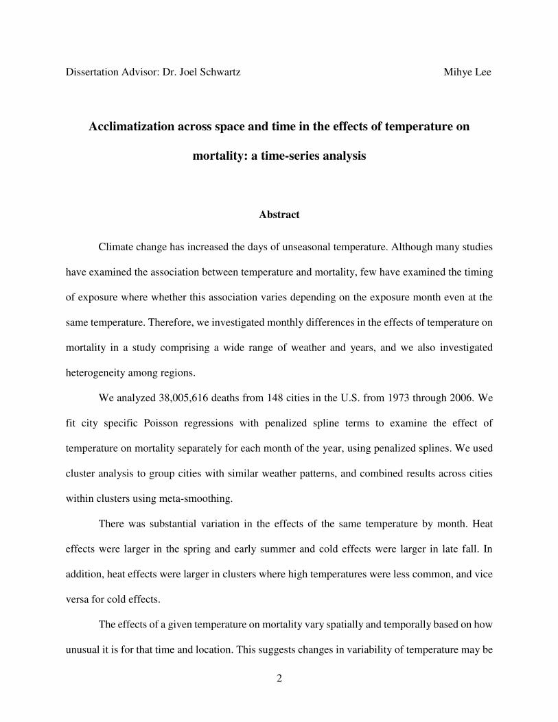
Dissertation Advisor: Dr. Joel Schwartz Mihye Lee

Acclimatization across space and time in the effects of temperature on

mortality: a time-series analysis

Abstract

Climate change has increased the days of unseasonal temperature. Although many studies

have examined the association between temperature and mortality, few have examined the timing

of exposure where whether this association varies depending on the exposure month even at the

same temperature. Therefore, we investigated monthly differences in the effects of temperature on

mortality in a study comprising a wide range of weather and years, and we also investigated

heterogeneity among regions.

We analyzed 38,005,616 deaths from 148 cities in the U.S. from 1973 through 2006. We

fit city specific Poisson regressions with penalized spline terms to examine the effect of

temperature on mortality separately for each month of the year, using penalized splines. We used

cluster analysis to group cities with similar weather patterns, and combined results across cities

within clusters using meta-smoothing.

There was substantial variation in the effects of the same temperature by month. Heat

effects were larger in the spring and early summer and cold effects were larger in late fall. In

addition, heat effects were larger in clusters where high temperatures were less common, and vice

versa for cold effects.

The effects of a given temperature on mortality vary spatially and temporally based on how

unusual it is for that time and location. This suggests changes in variability of temperature may be

3

more important for health as climate changes than changes of mean temperature. More emphasis

should be placed on warnings targeted to early heat/cold temperature for the season or month rather

than focusing only on the extremes.

4

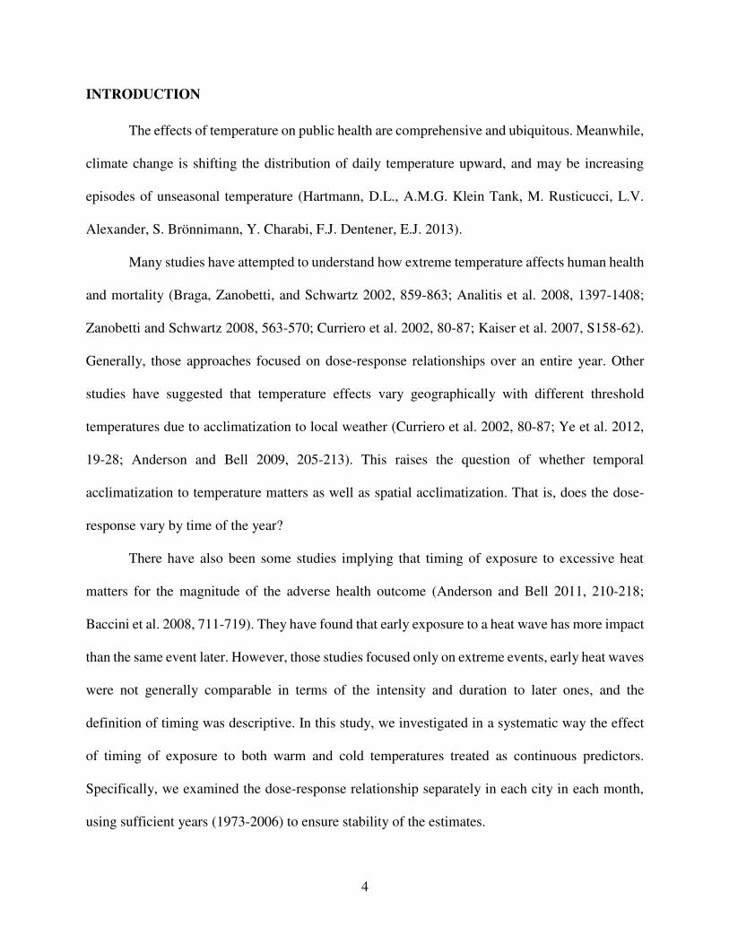
INTRODUCTION

The effects of temperature on public health are comprehensive and ubiquitous. Meanwhile,

climate change is shifting the distribution of daily temperature upward, and may be increasing

episodes of unseasonal temperature (Hartmann, D.L., A.M.G. Klein Tank, M. Rusticucci, L.V.

Alexander, S. Brönnimann, Y. Charabi, F.J. Dentener, E.J. 2013).

Many studies have attempted to understand how extreme temperature affects human health

and mortality (Braga, Zanobetti, and Schwartz 2002, 859-863; Analitis et al. 2008, 1397-1408;

Zanobetti and Schwartz 2008, 563-570; Curriero et al. 2002, 80-87; Kaiser et al. 2007, S158-62).

Generally, those approaches focused on dose-response relationships over an entire year. Other

studies have suggested that temperature effects vary geographically with different threshold

temperatures due to acclimatization to local weather (Curriero et al. 2002, 80-87; Ye et al. 2012,

19-28; Anderson and Bell 2009, 205-213). This raises the question of whether temporal

acclimatization to temperature matters as well as spatial acclimatization. That is, does the dose-

response vary by time of the year?

There have also been some studies implying that timing of exposure to excessive heat

matters for the magnitude of the adverse health outcome (Anderson and Bell 2011, 210-218;

Baccini et al. 2008, 711-719). They have found that early exposure to a heat wave has more impact

than the same event later. However, those studies focused only on extreme events, early heat waves

were not generally comparable in terms of the intensity and duration to later ones, and the

definition of timing was descriptive. In this study, we investigated in a systematic way the effect

of timing of exposure to both warm and cold temperatures treated as continuous predictors.

Specifically, we examined the dose-response relationship separately in each city in each month,

using sufficient years (1973-2006) to ensure stability of the estimates.

5

To further stabilize results we started with 148 US cities, and clustered them by similarity

in seasonal mean and variance of temperature to obtain clusters of cities with similar weather.

Results from cities belonging to the same cluster were combined to obtain a more robust estimate of

how temperature effect varies by month, and the resulting exposure-response curves were compared

among clusters. We also examined how the dose response curves varied by cluster, and the effect

of timing by cluster.

DATA

We obtained the data from 211 cities with complete mortality and weather variables for the

study. In most cases, a city was contained by a single county. However, we used multiple counties

where the city’s population extends beyond the boundaries of one county.

Among those cities, we restricted our analysis to cities with a daily average of 5 deaths per

day or more for statistical robustness. As a result, we ended up with 148 cities.

Meteorological data were downloaded from the National Oceanic and Atmospheric

Administration (NOAA) website and measured by airport weather stations. Since the data are from

the airport weather stations, the measurements included visibility in meters as well as daily mean

temperature, wind speed, sea level pressure, and dew point. Therefore, relative humidity was

calculated with the following formula:

Relative humidity (RH) = などど 抜 岾怠怠態貸待┻怠脹尼袋脹匂怠怠態袋待┻苔脹尼 峇腿

where Ta and Td denote air temperature and dew point temperature, respectively

(Wanielista, Kersten, and Eaglin 1997).

6

Among weather monitoring stations, the closest one in distance was assigned to each city

for ambient temperature and relative humidity. Since the weather stations were located in airports,

the difference in altitude didn’t play a role. In case a monitor has missing data, we used the values

of the nearest monitor within 60 kilometers. To remove erroneous readings without deleting true

extreme events, temperatures out of the 8 standard deviation range were eliminated.

Daily mortality data, including the number of deaths for each day and cause of death, were

obtained from the National Center for Health Statistics (NCHS), from the year 1973 through 2006

(Zanobetti and Schwartz 2008, 563-570; Zanobetti and Schwartz 2009, 898-903). We used deaths

from any natural cause except for accidental causes (ICD-code 10th revision: V01-Y98, ICD-code

9th revision: 1-799), of persons who resided within the city where they died.

METHOD

Considering the huge variations in the climate of the United States, we categorized the 148

cities into 8 statistical clusters by seasonal temperatures and their seasonal variances. By doing

this, we aimed to maximize the similarity within the cluster and dissimilarity between clusters at

the same time. Specifically, we employed an agglomerative hierarchical approach where, we

started by defining each data point to be a cluster and then combined existing clusters at each step

through the single linkage method. PROC CLUSTER in SAS 9.2 (Copyright © 2012 SAS Institute

Inc., SAS Campus Drive, Cary, North Carolina 27513, USA) was implemented based on the mean

and standard deviation of the temperature for four seasons in each city.

The statistical analysis consists of two phases. In the first stage, separate daily Poisson

time-series analyses were fit for each city and month of the year to evaluate the effect of

7

temperature on mortality. Because we had 34 years of data for each month, we had sufficient power

to estimate these effects. The effect of heat seems to primarily manifest within a day, whereas the

effect of cold temperatures is spread out over more days. To accommodate this we fit two

temperature variables, temperature on the day of death (lag 0), and the average temperature for the

five previous days (lags 1-5). For consistency, temperatures were centered to 18 °C. Since the

association of temperature with mortality can be nonlinear, we used a penalized spline to estimate

it. The model also controlled for the time trend of mortality and temperature over the 34 years by

adding a linear term on the sequence of days. To check the collinearity between the lag 0 lag 1-5,

the correlation coefficients were calculated. Day of week was also controlled. Specifically, we

assumed:

ln(ぢ)ijt = く0ij + く1iTimei + s(TMP0ijt) + s(TMP15ijt) + く2ijRHijt + く3DOWt,

where ぢ denotes the expected number of deaths on day t for city i in month j; Timei is the

sequence of days which counts within month and also increments with the calendar year in city i;

TMP0 is the ambient temperature in Celsius on the same day of death in city i; s is the penalized

spline function for the temperature effects, estimated with cubic regression splines with 10 knots;

TMP15 is the moving average of 1-5 previous days from the death day; RH is the relative humidity;

DOW is the indicator variable for day of week on day t. We assumed a quasi-Poisson distribution

for そ to account for any over-dispersion.

In the second stage, we combined the curves from the previous model into a curve

representing each month for each cluster. Doing this by cluster assured that the overlap in

temperature range between cities was large, and that the dose-response curves were similar. Since

the splines in the city specific models choose knot points based on the city specific distribution of

temperature, a meta-analysis of the spline coefficients is not possible. To avoid this problem, we

8

used meta-smoothing, a method introduced by Schwartz and Zanobetti to incorporate varying

smooth curves into one overall curve (Schwartz and Zanobetti 2000, 666-672). It is based on the

idea that predicted curves can be represented by using their predicted values for a dense range of

points. Using the predicted values at those points, and their variance, we can do a point-wise meta-

analysis.

In this study, we estimated predictions (and their confidence intervals) for each city/month

for each 2 °C interval. Next, we applied random effects meta-analyses for each temperature.

Finally, by connecting the points, meta-curves were completed. We confined the meta-smoothing

to the 99.9th percentile temperature range to avoid extreme values with only one city contributing

to the estimate. In the subgroup analysis, mortality due to respiratory disease was examined.

Humidity is a key factor for regulating the body temperature since it modifies the

evaporation of sweat in hot weather. As a sensitivity analysis to examine the effect of relative

humidity control, we reran the model without the relative humidity term.

Temperature effects may also be confounded by air pollution effects such as PM10 or PM2.5.

Since these were never measured in some cities, and only in later years in others, we analyzed

visibility instead as a surrogate for particles. Horizontal visibility is a sensitive indicator of fine

particle concentrations (Ozkaynak et al. 1986). And we repeated the meta-smoothing to compare

the results with one from the original model.

RESULTS

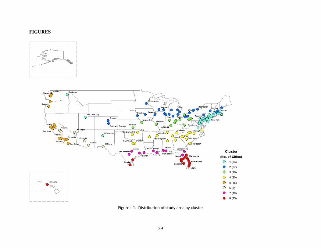
38,005,616 deaths occurred in 148 cities between 1973 and 2006. Figure I-1 and Table I-

1. show the location of 148 cities by cluster and the descriptive statistics of the temperature and

9

mortality. The first cluster consists of 36 cities mainly located along the northern Atlantic coast

area (New York City, Philadelphia, Boston, etc.) but also including some cities in the west

(Spokane, Salt Lake City, and Albuquerque). The second cluster (27 cities) was the coldest region

with cities such as Chicago, Detroit, and Minneapolis. The third cluster (16 cities), the secondly

coldest area, had cities such as Cleveland, Pittsburgh, and St. Louis. Cluster 4 is comprised of 20

warm cities with mild winter temperature such as Atlanta, Charlotte, and Dallas. Cluster 5 contains

16 cities along the west coast (Los Angeles, San Francisco, and Seattle). The sixth cluster consists

of 8 cities with very hot and dry weather such as Las Vegas and Phoenix. The seventh cluster is a

hot and humid area including 10 cities such as New Orleans, Austin, Houston, etc. Lastly, the

eighth cluster is made up of 15 tropical cities such as Miami and Honolulu.

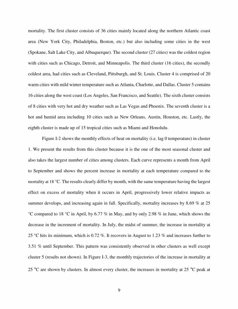
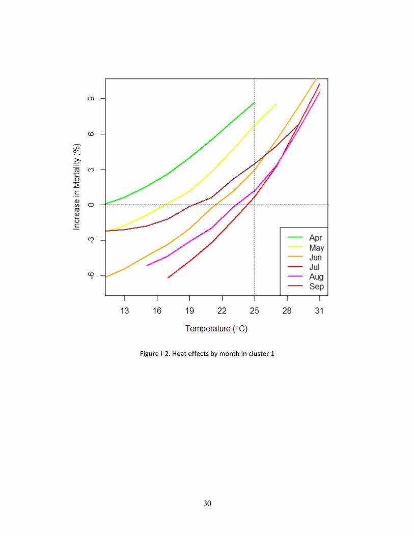
Figure I-2 shows the monthly effects of heat on mortality (i.e. lag 0 temperature) in cluster

1. We present the results from this cluster because it is the one of the most seasonal cluster and

also takes the largest number of cities among clusters. Each curve represents a month from April

to September and shows the percent increase in mortality at each temperature compared to the

mortality at 18 °C. The results clearly differ by month, with the same temperature having the largest

effect on excess of mortality when it occurs in April, progressively lower relative impacts as

summer develops, and increasing again in fall. Specifically, mortality increases by 8.69 % at 25

°C compared to 18 °C in April, by 6.77 % in May, and by only 2.98 % in June, which shows the

decrease in the increment of mortality. In July, the midst of summer, the increase in mortality at

25 °C hits its minimum, which is 0.72 %. It recovers in August to 1.23 % and increases further to

3.51 % until September. This pattern was consistently observed in other clusters as well except

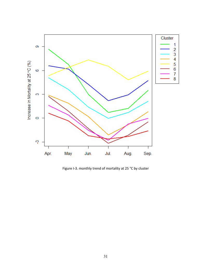
cluster 5 (results not shown). In Figure I-3, the monthly trajectories of the increase in mortality at

25 °C are shown by clusters. In almost every cluster, the increases in mortality at 25 °C peak at

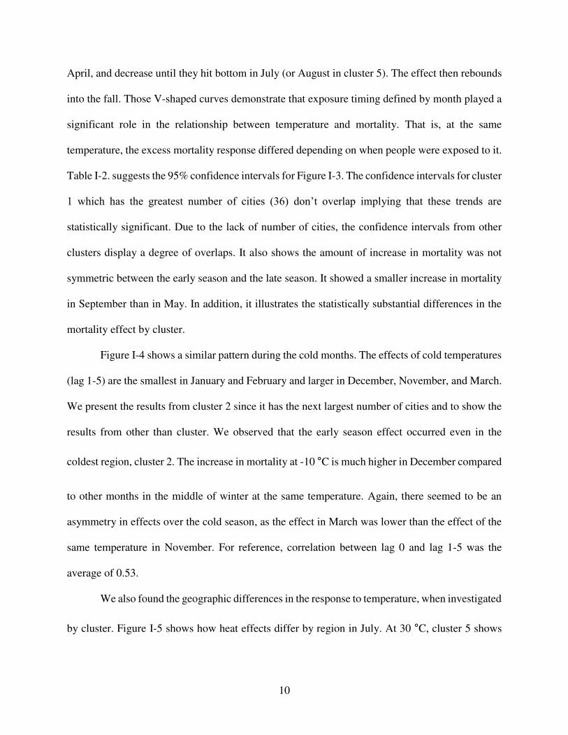
10

April, and decrease until they hit bottom in July (or August in cluster 5). The effect then rebounds

into the fall. Those V-shaped curves demonstrate that exposure timing defined by month played a

significant role in the relationship between temperature and mortality. That is, at the same

temperature, the excess mortality response differed depending on when people were exposed to it.

Table I-2. suggests the 95% confidence intervals for Figure I-3. The confidence intervals for cluster

1 which has the greatest number of cities (36) don’t overlap implying that these trends are

statistically significant. Due to the lack of number of cities, the confidence intervals from other

clusters display a degree of overlaps. It also shows the amount of increase in mortality was not

symmetric between the early season and the late season. It showed a smaller increase in mortality

in September than in May. In addition, it illustrates the statistically substantial differences in the

mortality effect by cluster.

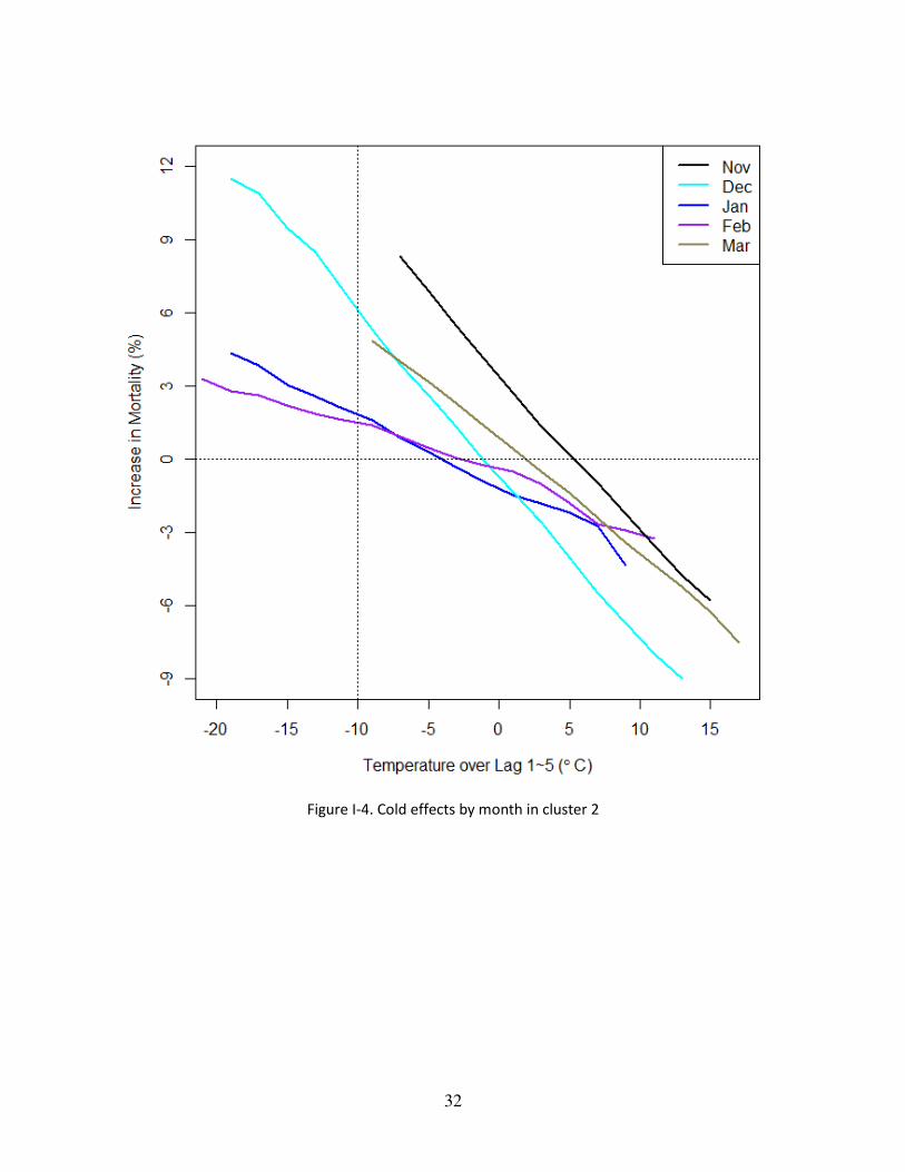
Figure I-4 shows a similar pattern during the cold months. The effects of cold temperatures

(lag 1-5) are the smallest in January and February and larger in December, November, and March.

We present the results from cluster 2 since it has the next largest number of cities and to show the

results from other than cluster. We observed that the early season effect occurred even in the

coldest region, cluster 2. The increase in mortality at -10 °C is much higher in December compared

to other months in the middle of winter at the same temperature. Again, there seemed to be an

asymmetry in effects over the cold season, as the effect in March was lower than the effect of the

same temperature in November. For reference, correlation between lag 0 and lag 1-5 was the

average of 0.53.

We also found the geographic differences in the response to temperature, when investigated

by cluster. Figure I-5 shows how heat effects differ by region in July. At 30 °C, cluster 5 shows

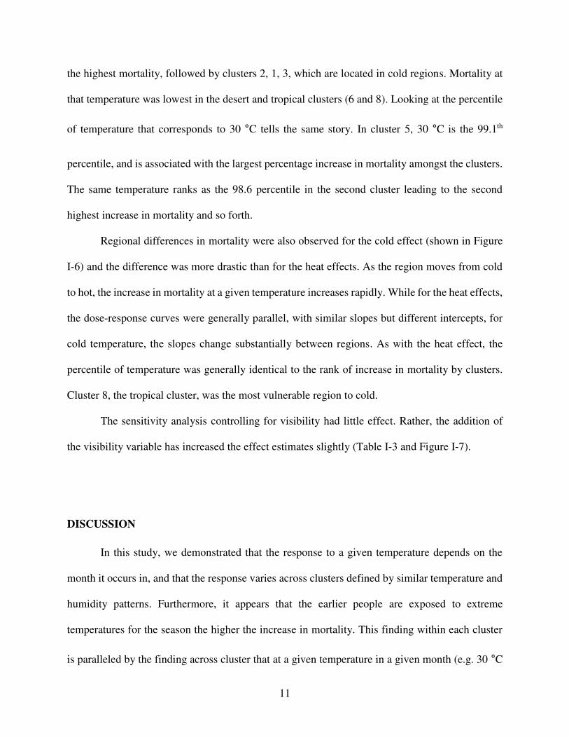
11

the highest mortality, followed by clusters 2, 1, 3, which are located in cold regions. Mortality at

that temperature was lowest in the desert and tropical clusters (6 and 8). Looking at the percentile

of temperature that corresponds to 30 °C tells the same story. In cluster 5, 30 °C is the 99.1th

percentile, and is associated with the largest percentage increase in mortality amongst the clusters.

The same temperature ranks as the 98.6 percentile in the second cluster leading to the second

highest increase in mortality and so forth.

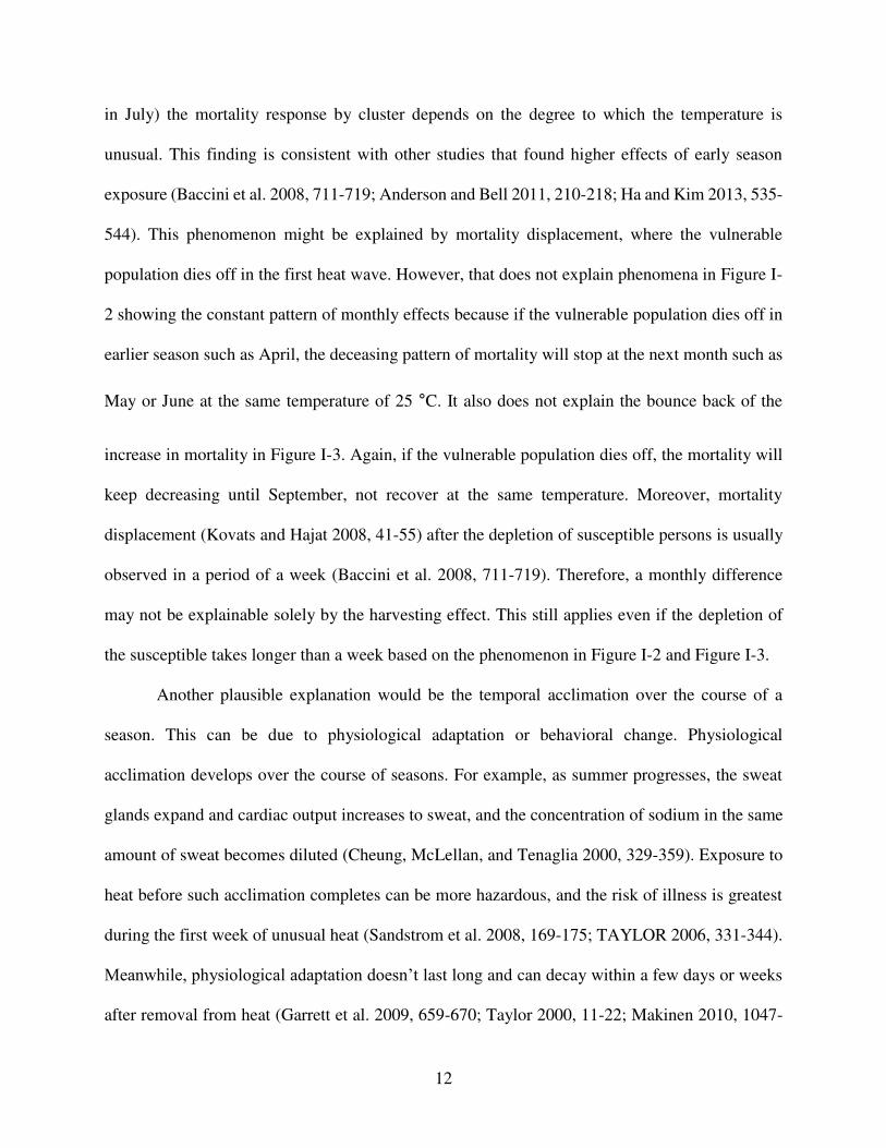
Regional differences in mortality were also observed for the cold effect (shown in Figure

I-6) and the difference was more drastic than for the heat effects. As the region moves from cold

to hot, the increase in mortality at a given temperature increases rapidly. While for the heat effects,

the dose-response curves were generally parallel, with similar slopes but different intercepts, for

cold temperature, the slopes change substantially between regions. As with the heat effect, the

percentile of temperature was generally identical to the rank of increase in mortality by clusters.

Cluster 8, the tropical cluster, was the most vulnerable region to cold.

The sensitivity analysis controlling for visibility had little effect. Rather, the addition of

the visibility variable has increased the effect estimates slightly (Table I-3 and Figure I-7).

DISCUSSION

In this study, we demonstrated that the response to a given temperature depends on the

month it occurs in, and that the response varies across clusters defined by similar temperature and

humidity patterns. Furthermore, it appears that the earlier people are exposed to extreme

temperatures for the season the higher the increase in mortality. This finding within each cluster

is paralleled by the finding across cluster that at a given temperature in a given month (e.g. 30 °C

12

in July) the mortality response by cluster depends on the degree to which the temperature is

unusual. This finding is consistent with other studies that found higher effects of early season

exposure (Baccini et al. 2008, 711-719; Anderson and Bell 2011, 210-218; Ha and Kim 2013, 535-

544). This phenomenon might be explained by mortality displacement, where the vulnerable

population dies off in the first heat wave. However, that does not explain phenomena in Figure I-

2 showing the constant pattern of monthly effects because if the vulnerable population dies off in

earlier season such as April, the deceasing pattern of mortality will stop at the next month such as

May or June at the same temperature of 25 °C. It also does not explain the bounce back of the

increase in mortality in Figure I-3. Again, if the vulnerable population dies off, the mortality will

keep decreasing until September, not recover at the same temperature. Moreover, mortality

displacement (Kovats and Hajat 2008, 41-55) after the depletion of susceptible persons is usually

observed in a period of a week (Baccini et al. 2008, 711-719). Therefore, a monthly difference

may not be explainable solely by the harvesting effect. This still applies even if the depletion of

the susceptible takes longer than a week based on the phenomenon in Figure I-2 and Figure I-3.

Another plausible explanation would be the temporal acclimation over the course of a

season. This can be due to physiological adaptation or behavioral change. Physiological

acclimation develops over the course of seasons. For example, as summer progresses, the sweat

glands expand and cardiac output increases to sweat, and the concentration of sodium in the same

amount of sweat becomes diluted (Cheung, McLellan, and Tenaglia 2000, 329-359). Exposure to

heat before such acclimation completes can be more hazardous, and the risk of illness is greatest

during the first week of unusual heat (Sandstrom et al. 2008, 169-175; TAYLOR 2006, 331-344).

Meanwhile, physiological adaptation doesn’t last long and can decay within a few days or weeks

after removal from heat (Garrett et al. 2009, 659-670; Taylor 2000, 11-22; Makinen 2010, 1047-

13

1067). This may explain the bounce back of mortality in Figure I-3. The non-symmetry in the

amount of the increase in mortality between the early season and the late season may be explained

by the remaining effects of acclimation. Behavioral adaptation such as wearing more clothes or

the use of air conditioners is another key factor for lowering mortality. However, early exposure

to heat/cold might occur before behavioral adaptation. The public may neglect to prepare

themselves for early heat or cold, compared to those in the middle of season. The public should be

notified that 25 °C in May can be as harmful to health as 29 °C in July.

For cold, there were more cumulative effects defined by lag 1 through lag 5. This could be

because mortality due to cold is indirect, through illnesses such as pneumonia and influenza

(McGeehin and Mirabelli 2001, 185-189). Mortality due to respiratory causes also showed a huge

difference between the induction of the season (December) and the middle of the season

(February). And it appears that the retention of acclimation lasts longer for cold than heat,

considering that February showed the lowest mortality whereas July had the lowest mortality effect

in summer.

Our findings suggest that if the effects of temperature are highly time dependent (i.e., differ

by specific month), investigating temperature by season or only by year effectively averages over

diverse months. Therefore, summing up temperature effects and ignoring the timing would dilute

the effects of ambient temperature, reducing the estimated change in mortality per unit change in

temperature.

We also found that spatial differences in the temperature effect on mortality. Cluster 6,

characterized by a hot and dry climate, showed the strongest resistance to the heat. The first

possible hypothesis is that the low relative humidity in those dry areas contributed to this high

resistance to the heat. It appears that heat acclimation remains longer for dry heat compared to

14

humid heat (Pandolf 1998, S157-60). It could also be due to the prevalence of air conditioning.

Lastly, compared to cluster 8, which is a tropical region, a wider range of heat temperature may

have provoked the adaptation to the variability of temperature. For cold, the regional difference

was greater than the heat effects. This suggests that human adapt better to cold than to heat.

Removal of the relative humidity from the model made estimates for early summer

decrease but increases estimates for late season and winter. This might imply the adaptation is also

going on for humidity as well as temperature.

Our results were not confounded by visibility, which is a surrogate measurement of

particulate matter such as PM10 and PM2.5. Rather, the addition of visibility increased the model

estimates for temperature. Other studies also state that the relationship between temperature-

mortality is robust to air pollution control (Zanobetti and Schwartz 2008, 563-570; Anderson and

Bell 2009, 205-213).

The main limitation of the study is the use of ambient temperature as a surrogate for

personal exposure. Personal exposure to ambient temperature is modified by adaptive mechanisms

such as use of air conditioning. Actual outdoor temperature also can be altered from the airport

monitoring stations due to the distance from the monitors and the difference in topography and

elevation. Nevertheless, our results are conservative, because the measurement error is non-

differential to the outcome. With an ongoing attempt to precisely predict temperature (Kloog et al.

2012, 85-92), exposure measurements will be improved.

Since cardiovascular stability is critical in heat acclimation and is also affected by cold,

compromises in this ability will pose more severe burdens on the elderly and the ill. In future

studies, subgroup analyses for these populations will reveal more about the impact of monthly

temperature anomalies.

15

Our study has many policy implications. The monthly effects of temperature suggest that

more warnings should be given to the public for hot and cold events early in the season as they

occur before acclimation has developed. The media and many studies are interested in peak

temperatures such as 40°C in the middle of summer. Yet our findings indicate that the impact of

early events of less extreme temperature may be greater. Also, warnings could be provided based

on a relative scale, such as a percentile, as well as the absolute scale of temperature. In July, 25°C

is merely the 49th percentile, whereas the same temperature is the 86th percentile in May, and it

poses more harm to the public in the earlier season. To the extent that climate change increases the

occurrence of early season warm or cold days, this may be an important health consequence of

such changes.

To our knowledge, this is the first study to examine the dependence on month of the effects

of temperature on mortality. Timing of exposure to extreme temperature should be given more

attention in terms of acclimation. Early heat and cold pose a higher risk, as people are not prepared

for them. Furthermore, due to climate change, it is projected that unseasonal days will be increasing

and arriving earlier. It is necessary to prepare for these hazards.

16

Bibliography

Alston, E. J., I. N. Sokolik, and O. V. Kalashnikova. 2012. "Characterization of Atmospheric

Aerosol in the US Southeast from Ground- and Space-Based Measurements Over the Past

Decade." Atmospheric Measurement Techniques 5 (7): 1667-1682.

Analitis, A., K. Katsouyanni, A. Biggeri, M. Baccini, B. Forsberg, L. Bisanti, U. Kirchmayer, et

al. 2008. "Effects of Cold Weather on Mortality: Results from 15 European Cities within the

PHEWE Project." American Journal of Epidemiology 168 (12): 1397-1408.

Anderson, B. G. and M. L. Bell. 2009. "Weather-Related Mortality: How Heat, Cold, and Heat

Waves Affect Mortality in the United States." Epidemiology (Cambridge, Mass.) 20 (2): 205-

213.

Anderson, G. B. and M. L. Bell. 2011. "Heat Waves in the United States: Mortality Risk during

Heat Waves and Effect Modification by Heat Wave Characteristics in 43 U.S. Communities."

Environmental Health Perspectives 119 (2): 210-218.

Armstrong, B. G. 1998. "Effect of Measurement Error on Epidemiological Studies of

Environmental and Occupational Exposures." Occupational and Environmental Medicine 55

(10): 651-656.

Baccini, M., A. Biggeri, G. Accetta, T. Kosatsky, K. Katsouyanni, A. Analitis, H. R. Anderson, et

al. 2008. "Heat Effects on Mortality in 15 European Cities." Epidemiology (Cambridge, Mass.)

19 (5): 711-719.

17

Barnett, A. G., G. M. Williams, J. Schwartz, T. L. Best, A. H. Neller, A. L. Petroeschevsky, and

R. W. Simpson. 2006. "The Effects of Air Pollution on Hospitalizations for Cardiovascular

Disease in Elderly People in Australian and New Zealand Cities." Environmental Health

Perspectives 114 (7): 1018-1023.

Beckerman, Bernardo S., Michael Jerrett, Randall V. Martin, Aaron van Donkelaar, Zev Ross, and

Richard T. Burnett. 2013. "Application of the Deletion/Substitution/Addition Algorithm to

Selecting Land use Regression Models for Interpolating Air Pollution Measurements in

California." Atmospheric Environment 77 (0): 172-177.

Boldo, Elena, Sylvia Medina, Alain Le Tertre, Fintan Hurley, Hans-Guido Mücke, Ferrán

Ballester, and Inmaculada Aguilera. 2006. "Apheis: Health Impact Assessment of Long-Term

Exposure to PM2.5 in 23 European Cities." European Journal of Epidemiology 21 (6): 449-

458.

Braga, A. L., A. Zanobetti, and J. Schwartz. 2002. "The Effect of Weather on Respiratory and

Cardiovascular Deaths in 12 U.S. Cities." Environmental Health Perspectives 110 (9): 859-

863.

Brenner, H., D. A. Savitz, K. H. Jockel, and S. Greenland. 1992. "Effects of Nondifferential

Exposure Misclassification in Ecologic Studies." American Journal of Epidemiology 135 (1):

85-95.

Cheung, S. S., T. M. McLellan, and S. Tenaglia. 2000. "The Thermophysiology of Uncompensable

Heat Stress. Physiological Manipulations and Individual Characteristics." Sports Medicine

(Auckland, N.Z.) 29 (5): 329-359.

18

Cormier, S. A., S. Lomnicki, W. Backes, and B. Dellinger. 2006. "Origin and Health Impacts of

Emissions of Toxic by-Products and Fine Particles from Combustion and Thermal Treatment

of Hazardous Wastes and Materials." Environmental Health Perspectives 114 (6): 810-817.

Curriero, F. C., K. S. Heiner, J. M. Samet, S. L. Zeger, L. Strug, and J. A. Patz. 2002. "Temperature

and Mortality in 11 Cities of the Eastern United States." American Journal of Epidemiology

155 (1): 80-87.

de Hoogh, Kees, Meng Wang, Martin Adam, Chiara Badaloni, Rob Beelen, Matthias Birk, Giulia

Cesaroni, et al. 2013. "Development of Land use Regression Models for Particle Composition

in Twenty Study Areas in Europe." Environmental Science & Technology 47 (11): 5778-5786.

Dockery, D. W. 2009. "Health Effects of Particulate Air Pollution." Annals of Epidemiology 19

(4): 257-263.

Dockery, Douglas W., C. A. Pope, Xiping Xu, John D. Spengler, James H. Ware, Martha E. Fay,

Benjamin G. Ferris, and Frank E. Speizer. 1993. "An Association between Air Pollution and

Mortality in Six U.S. Cities." N Engl J Med 329 (24): 1753-1759.

Franklin, Meredith, Ariana Zeka, and Joel Schwartz. 2006. "Association between PM2.5 and all-

Cause and Specific-Cause Mortality in 27 US Communities." J Expos Sci Environ Epidemiol

17 (3): 279-287.

Garrett, A. T., N. G. Goosens, N. J. Rehrer, M. J. Patterson, and J. D. Cotter. 2009. "Induction and

Decay of Short-Term Heat Acclimation." European Journal of Applied Physiology 107 (6):

659-670.

19

Goldman, G. T., J. A. Mulholland, A. G. Russell, M. J. Strickland, M. Klein, L. A. Waller, and P.

E. Tolbert. 2011. "Impact of Exposure Measurement Error in Air Pollution Epidemiology:

Effect of Error Type in Time-Series Studies." Environmental Health : A Global Access

Science Source 10: 61-069X-10-61.

Greenland, S. 1992. "Divergent Biases in Ecologic and Individual-Level Studies." Statistics in

Medicine 11 (9): 1209-1223.

Ha, J. and H. Kim. 2013. "Changes in the Association between Summer Temperature and Mortality

in Seoul, South Korea." International Journal of Biometeorology 57 (4): 535-544.

Hartmann, D.L., A.M.G. Klein Tank, M. Rusticucci, L.V. Alexander, S. Brönnimann, Y. Charabi,

F.J. Dentener, E.J. 2013. 2013: Observations:<br />Atmosphere and Surface. in: Climate

Change 2013: The Physical Science Basis. Contribution of Working Group<br />I to the

Fifth Assessment Report of the Intergovernmental Panel on Climate Change [Stocker, T.F.,

D. Qin, G.-K.<br />Plattner, M. Tignor, S.K. Allen, J. Boschung, A. Nauels, Y. Xia, V. Bex

and P.M. Midgley (Eds.)] . Cambridge, United Kingdom and New York, NY, USA:

Cambridge University.

Hu, Xuefei, Lance A. Waller, Alexei Lyapustin, Yujie Wang, Mohammad Z. Al-Hamdan, William

L. Crosson, Maurice G. Estes Jr., et al. 2014. "Estimating Ground-Level PM2.5

Concentrations in the Southeastern United States using MAIAC AOD Retrievals and a Two-

Stage Model." Remote Sensing of Environment 140 (0): 220-232.

20

Jin, Suming, Limin Yang, Patrick Danielson, Collin Homer, Joyce Fry, and George Xian. 2013.

"A Comprehensive Change Detection Method for Updating the National Land Cover

Database to Circa 2011." Remote Sensing of Environment 132 (0): 159-175.

Kaiser, R., A. Le Tertre, J. Schwartz, C. A. Gotway, W. R. Daley, and C. H. Rubin. 2007. "The

Effect of the 1995 Heat Wave in Chicago on all-Cause and Cause-Specific Mortality."

American Journal of Public Health 97 Suppl 1: S158-62.

Kloog, I., A. Chudnovsky, P. Koutrakis, and J. Schwartz. 2012. "Temporal and Spatial

Assessments of Minimum Air Temperature using Satellite Surface Temperature

Measurements in Massachusetts, USA." The Science of the Total Environment 432: 85-92.

Kloog, I., F. Nordio, A. Zanobetti, B. A. Coull, P. Koutrakis, and J. D. Schwartz. 2014. "Short

Term Effects of Particle Exposure on Hospital Admissions in the Mid-Atlantic States: A

Population Estimate." PloS One 9 (2): e88578.

Kloog, Itai, Petros Koutrakis, Brent A. Coull, Hyung Joo Lee, and Joel Schwartz. 2011. "Assessing

Temporally and Spatially Resolved PM2.5 Exposures for Epidemiological Studies using

Satellite Aerosol Optical Depth Measurements." Atmospheric Environment 45 (35): 6267-

6275.

Kovats, R. S. and S. Hajat. 2008. "Heat Stress and Public Health: A Critical Review." Annual

Review of Public Health 29: 41-55.

21

Lee, H. J., Y. Liu, B. A. Coull, J. Schwartz, and P. Koutrakis. 2011. "A Novel Calibration

Approach of MODIS AOD Data to Predict PM$_2.5$ Concentrations." Atmospheric

Chemistry and Physics 11 (15): 7991-8002.

Li, Xia, Xiangao Xia, Shengli Wang, Jietai Mao, and Yan Liu. 2012. "Validation of MODIS and

Deep Blue Aerosol Optical Depth Retrievals in an Arid/Semi-Arid Region of Northwest

China." Particuology 10 (1): 132-139.

Lyapustin, A., Y. Wang, I. Laszlo, R. Kahn, S. Korkin, L. Remer, R. Levy, and J. S. Reid. 2011.

"Multiangle Implementation of Atmospheric Correction (MAIAC): 2. Aerosol Algorithm."

Journal of Geophysical Research: Atmospheres 116 (D3): - D03211.

Maclure, M. 1991. "The Case-Crossover Design: A Method for Studying Transient Effects on the

Risk of Acute Events." American Journal of Epidemiology 133 (2): 144-153.

Makinen, T. M. 2010. "Different Types of Cold Adaptation in Humans." Frontiers in Bioscience

(Scholar Edition) 2: 1047-1067.

Mar, Therese F., Kazuhiko Ito, Jane Q. Koenig, Timothy V. Larson, Delbert J. Eatough, Ronald

C. Henry, Eugene Kim, et al. 2005. "PM Source Apportionment and Health Effects. 3.

Investigation of Inter-Method Variations in Associations between Estimated Source

Contributions of PM2.5 and Daily Mortality in Phoenix, AZ." J Expos Sci Environ Epidemiol

16 (4): 311-320.

22

McGeehin, M. A. and M. Mirabelli. 2001. "The Potential Impacts of Climate Variability and

Change on Temperature-Related Morbidity and Mortality in the United States."

Environmental Health Perspectives 109 Suppl 2: 185-189.

Medina-Ramon, M. and J. Schwartz. 2007. "Temperature, Temperature Extremes, and Mortality:

A Study of Acclimatisation and Effect Modification in 50 US Cities." Occupational and

Environmental Medicine 64 (12): 827-833.

Ostro, B. D., R. Broadwin, and M. J. Lipsett. 2000. "Coarse and Fine Particles and Daily Mortality

in the Coachella Valley, California: A Follow-Up Study." Journal of Exposure Analysis and

Environmental Epidemiology 10 (5): 412-419.

Pandolf, K. B. 1998. "Time Course of Heat Acclimation and its Decay." International Journal of

Sports Medicine 19 Suppl 2: S157-60.

Pope, C. A.,3rd. 2000. "Epidemiology of Fine Particulate Air Pollution and Human Health:

Biologic Mechanisms and Who's at Risk?" Environmental Health Perspectives 108 Suppl 4:

713-723.

Pope, C. A.,3rd, R. T. Burnett, M. J. Thun, E. E. Calle, D. Krewski, K. Ito, and G. D. Thurston.

2002. "Lung Cancer, Cardiopulmonary Mortality, and Long-Term Exposure to Fine

Particulate Air Pollution." JAMA : The Journal of the American Medical Association 287 (9):

1132-1141.

23

Rhomberg, L. R., J. K. Chandalia, C. M. Long, and J. E. Goodman. 2011. "Measurement Error in

Environmental Epidemiology and the Shape of Exposure-Response Curves." Critical Reviews

in Toxicology 41 (8): 651-671.

Risom, L., P. Moller, and S. Loft. 2005. "Oxidative Stress-Induced DNA Damage by Particulate

Air Pollution." Mutation Research 592 (1-2): 119-137.

Ruchirawat, M., D. Settachan, P. Navasumrit, J. Tuntawiroon, and H. Autrup. 2007. "Assessment

of Potential Cancer Risk in Children Exposed to Urban Air Pollution in Bangkok, Thailand."

Toxicology Letters 168 (3): 200-209.

Ryan, P. H. and G. K. LeMasters. 2007. "A Review of Land-use Regression Models for

Characterizing Intraurban Air Pollution Exposure." Inhalation Toxicology 19 Suppl 1: 127-

133.

Samet, J. M., F. Dominici, F. C. Curriero, I. Coursac, and S. L. Zeger. 2000. "Fine Particulate Air

Pollution and Mortality in 20 U.S. Cities, 1987-1994." The New England Journal of Medicine

343 (24): 1742-1749.

Sandstrom, M. E., J. C. Siegler, R. J. Lovell, L. A. Madden, and L. McNaughton. 2008. "The Effect

of 15 Consecutive Days of Heat-Exercise Acclimation on Heat Shock Protein 70." Cell Stress

& Chaperones 13 (2): 169-175.

Schwartz, J. and A. Zanobetti. 2000. "Using Meta-Smoothing to Estimate Dose-Response Trends

Across Multiple Studies, with Application to Air Pollution and Daily Death." Epidemiology

(Cambridge, Mass.) 11 (6): 666-672.

24

TAYLOR, Nigel A. S. 2006. "Challenges to Temperature Regulation when Working in Hot

Environments." Industrial Health 44 (3): 331-344.

Taylor, Nigel A. S. 2000. "Principles and Practices of Heat Adaptation." Journal of the Human-

Environment System 4 (1): 11-22.

Valavanidis, A., K. Fiotakis, and T. Vlachogianni. 2008. "Airborne Particulate Matter and Human

Health: Toxicological Assessment and Importance of Size and Composition of Particles for

Oxidative Damage and Carcinogenic Mechanisms." Journal of Environmental Science and

Health.Part C, Environmental Carcinogenesis & Ecotoxicology Reviews 26 (4): 339-362.

Wang, Rongrong, Sarah B. Henderson, Hind Sbihi, Ryan W. Allen, and Michael Brauer. 2013.

"Temporal Stability of Land use Regression Models for Traffic-Related Air Pollution."

Atmospheric Environment 64 (0): 312-319.

Wanielista, Martin P., Robert Kersten, and Ron Eaglin. 1997. Hydrology : Water Quantity and

Quality Control. 2nd ed. New York: John Wiley & Sons.

Whitworth, K. W., E. Symanski, D. Lai, and A. L. Coker. 2011. "Kriged and Modeled Ambient

Air Levels of Benzene in an Urban Environment: An Exposure Assessment Study."

Environmental Health : A Global Access Science Source 10: 21-069X-10-21.

Wichmann, H. E., C. Spix, T. Tuch, G. Wölke, A. Peters, J. Heinrich, W. G. Kreyling, and J.

Heyder. 2000. "Daily Mortality and Fine and Ultrafine Particles in Erfurt, Germany Part I:

Role of Particle Number and Particle Mass." Research Report (Health Effects Institute) (98):

5-86; discussion 87-94.

25

Ye, X., R. Wolff, W. Yu, P. Vaneckova, X. Pan, and S. Tong. 2012. "Ambient Temperature and

Morbidity: A Review of Epidemiological Evidence." Environmental Health Perspectives 120

(1): 19-28.

Zanobetti, A. and J. Schwartz. 2009. "The Effect of Fine and Coarse Particulate Air Pollution on

Mortality: A National Analysis." Environmental Health Perspectives 117 (6): 898-903.

———. 2008. "Temperature and Mortality in Nine US Cities." Epidemiology (Cambridge, Mass.)

19 (4): 563-570.

26

TABLES

Table I-1. Descriptive Statistics of Temperature and Mortality by Cluster

Cluster Season Temperature (°C) Relative Humidity (%) Daily Death (Count)

Mean

S.D.* Mean S.D. Mean S.D.

1

Spring-Summer 16.83 8.00 63.55 16.84 22.63 33.08

Fall-Winter 7.03 8.53 66.20 15.41 24.29 35.57

2 Spring-Summer 15.12 8.63 65.12 14.97 19.00 28.11

Fall-Winter 4.13 9.56 69.76 14.33 20.22 29.88

3 Spring-Summer 18.04 8.16 65.77 13.43 17.29 13.67

Fall-Winter 7.03 9.38 69.47 13.18 18.43 14.56

4 Spring-Summer 21.10 6.74 65.86 13.92 12.33 9.07

Fall-Winter 11.58 8.14 66.82 15.52 13.20 9.70

5 Spring-Summer 16.79 4.93 66.56 13.83 29.16 33.50

Fall-Winter 12.83 5.65 70.42 17.25 31.16 36.35

6 Spring-Summer 23.67 7.09 37.35 17.40 13.50 12.50

Fall-Winter 14.76 7.36 52.66 21.91 14.51 13.40

7 Spring-Summer 23.93 5.01 70.99 12.20 13.47 11.58

Fall-Winter 16.69 6.99 71.13 14.42 14.34 12.28

8 Spring-Summer 25.29 3.63 71.52 9.69 15.61 11.76

Fall-Winter 21.02 5.44 73.13 10.87 16.39 12.22

*S.D. is the standard deviation

27

Table I-2. Percent increase in Mortality at 25 °C by Cluster and Month

April May June July August September

8.69 (7.16, 10.25) 6.77 (5.52, 8.04) 2.98 (2.57, 3.39) 0.72 (0.48, 0.96) 1.23 (0.90, 1.57) 3.51 (2.77, 4.26)

6.58 (4.63, 8.56) 6.19 (4.94, 7.46) 4.26 (3.53, 4.99) 2.20 (1.78, 2.62) 2.92 (2.29, 3.56) 4.74 (3.67, 5.81)

5.09 (3.21, 7.01) 3.60 (2.70, 4.51) 1.39 (0.99, 1.80) -0.02 (-0.13, 0.09) 0.70 (0.46, 0.94) 2.13 (1.30, 2.97)

2.89 (1.68, 4.12) 1.87 (1.10, 2.65) 0.19 (0.04, 0.35) -2.10 (-2.87, -1.33) -0.82 (-1.16, -0.48) 0.82 (0.31, 1.33)

5.35 (1.34, 9.51) 6.40 (4.07, 8.79) 7.33 (4.89, 9.82) 6.52 (5.21, 7.85) 4.82 (2.99, 6.69) 5.93 (3.95, 7.95)

2.74 (1.03, 4.49) 0.88 (0.36, 1.39) -1.31 (-2.06, -0.54) -3.19 (-6.26, -0.02) -2.14 (-3.57, -0.70) -0.49 (-0.77, -0.21)

1.62 (0.38, 2.87) 0.39 (0.04, 0.75) -1.54 (-2.25, -0.81) -2.8 (-4.30, -1.26) -0.74 (-2.06, 0.61) -0.02 (-0.25, 0.20)

0.61 (0.11, 1.11) -0.36 (-0.62, -0.10) -2.22 (-3.12, -1.31) -2.63 (-4.05, -1.20) -2.30 (-3.73, -0.85) -1.59 (-2.61, -0.56)

Estimate is percent increase in mortality at 25 °C compared to mortality at 18 °C Negative value means lower mortality than the reference temperature of 18 °C. () is 95% confidence interval

28

Table I-3. Sensitivity Analysis に Percent Increase in Mortality at 25 °C by Cluster and Month

April May June July August September

9.04 (7.42, 10.68) 7.02 (5.60, 8.47) 2.79 (2.27, 3.32) 0.66 (0.41, 0.91) 1.25 (0.92, 1.59) 3.45 (2.69, 4.21)

6.48 (4.56, 8.43) 6.00 (4.78, 7.24) 4.08 (3.25, 4.92) 1.98 (1.53, 2.44) 2.63 (1.94, 3.31) 4.38 (3.19, 5.58)

4.88 (2.98, 6.82) 3.72 (2.80, 4.65) 1.50 (1.06, 1.94) -0.03 (-0.15, 0.09) 0.61 (0.33, 0.88) 2.08 (1.15, 3.02)

2.93 (1.75, 4.13) 1.65 (0.80, 2.52) 0.22 (0.05, 0.38) -1.93 (-2.70, -1.15) -0.74 (-1.14, -0.35) 0.77 (0.27, 1.28)

5.58 (1.22, 10.14) 6.69 (4.41, 9.02) 7.24 (4.74, 9.79) 6.29 (4.90, 7.69) 4.33 (2.80, 5.88) 6.18 (4.17, 8.23)

2.82 (0.60, 5.10) 0.64 (0.06, 1.22) -1.43 (-2.21, -0.65) -3.91 (-6.76, -0.97) -2.40 (-3.84, -0.94) -0.51 (-0.78, -0.24)

1.64 (0.13, 3.18) 0.38 (0.01, 0.74) -1.48 (-2.25, -0.70) -2.74 (-4.25, -1.20) -0.64 (-1.98, 0.72) -0.04 (-0.27, 0.19)

0.65 (0.09, 1.21) -0.38 (-0.62, -0.14) -2.05 (-2.95, -1.14) -2.56 (-3.96, -1.15) -2.40 (-3.90, -0.88) -1.42 (-2.30, -0.52)

Sensitivity analysis for the addition of visibility. Estimate is percent increase in mortality at 25 °C compared to mortality at the mean of each cluster and month Negative value means lower mortality than the reference temperature of 18 °C. () is 95% confidence interval

29

FIGURES

Figure I-1. Distribution of study area by cluster

30

Figure I-2. Heat effects by month in cluster 1

31

Figure I-3. monthly trend of mortality at 25 °C by cluster

32

Figure I-4. Cold effects by month in cluster 2

33

Figure I-5. Heat effects in July by cluster

34

Figure I-6. Cold effects in January by cluster

35

Figure I-7. Sensitivity analysis on visibility

36

CHAPTER II

Spatiotemporal prediction of fine particulate matter using high resolution

satellite images in the southeastern U.S 2003-2011

Mihye Lee1, Itai Kloog2, Alexandra Chudnovsky3, Alexei Lyapustin4, Yujie Wang5, Steven

Melly6, Brent Coull7, Petros Koutrakis1, Joel Schwartz1

1Exposure, Epidemiology, and Risk Program, Department of Environmental Health, Harvard

School of Public Health, Boston, MA, USA

2Department of Geography and Environmental Development, Ben-Gurion University of the

Negev, Beer Sheva, Israel

3Department of Geography and Human Environment, Tel-Aviv University, Israel

4GEST/UMBC, NASA Goddard Space Flight Center, Baltimore, MD, USA

5Goddard Earth Sciences and Technology center, University of Maryland Baltimore County,

Baltimore, MD, USA

6Department of Epidemiology and Biostatistics, Drexel University School of Public Health, Philadelphia, PA, USA

7Department of Biostatistics, Harvard School of Public Health, Boston, MA, USA

37

Dissertation Advisor: Dr. Joel Schwartz Mihye Lee

Spatiotemporal prediction of fine particulate matter

using high resolution satellite images in the southeastern U.S 2003-2011

Abstract

Most studies have demonstrated that fine particulate matter (PM2.5, particles smaller than

2.5 たm in aerodynamic diameter) is associated with adverse health outcomes. The use of ground

monitoring stations of PM2.5 to approximate personal exposure however, induces measurement

error. Land use regression provides spatially resolved predictions but land use terms do not vary

temporally. Meanwhile, the advent of satellite-retrieved aerosol optical depth (AOD) products

have made spatiotemporally-resolved PM2.5 predictions possible.

In this paper, we incorporated AOD satellite measurements with other predictors such as

meteorological variables, land use regression, and spatial smoothing to predict the daily

concentration of PM2.5 at a 1 km2 resolution across the southeastern United States covering the

seven states of Georgia, North Carolina, South Carolina, Alabama, Tennessee, Mississippi, and

Florida for the years from 2003 through 2011. We divided the extensive study area into 3 regions

and applied separate mixed-effect models to calibrate AOD values to PM2.5 with other

spatiotemporal predictors.

Using 10-fold cross-validation, we obtained out of sample R2 of 0.77, 0.81, and 0.70 with

the square root of the mean squared prediction errors (RMSPE) of 2.89 たg/m3, 2.51 たg/m3, and

38

2.82 たg/m3 for regions 1, 2, and 3, respectively. The slopes of the relationships between predicted

PM2.5 and held out measurements were near 1 indicating no bias in the prediction model.

In conclusion, satellite AOD measurements can be combined with traditional land use

terms to provide spatiotemporal predictions of PM2.5 at a 1 km scale. These predictions can be

used in epidemiological studies investigating the effects of both acute and chronic exposures to

PM2.5. Our model results will also extend the existing studies on PM2.5 which are generally targeted

to largely urban areas due to the availability of monitoring, into areas not previously studied such

as rural areas.

39

INTRODUCTION

Particulate matter (PM) is particles or aerosols suspended in the atmosphere in various

forms such as smoke, dust, or water droplets. The source of those aerosols are diverse including

natural sources such as wild fire, sea particles, natural dust, and anthropogenic sources such as

vehicles, houses, power plants or industrial factories. Among the various sizes of particulate

matter, fine particulate matter (particulate matter with aerodynamic diameter < 2.5 たm, PM2.5)

poses the greatest health risks since it mainly originates from incomplete combustion and its small

size allows it to penetrate through the human defense system, and into the systematic circulation

system (Cormier et al. 2006, 810-817).

Since the Six Cities study (Dockery et al. 1993, 1753-1759), which showed a strong linear

relationship between PM2.5 and mortality between cities that differed by pollution level, a body of

literature has developed reporting associations between PM2.5 and adverse health effects ranging

from respiratory or cardiovascular diseases to increases in hospital admissions and death (Pope

2000, 713-723; Pope et al. 2002, 1132-1141; Barnett et al. 2006, 1018-1023). In many of those

studies, the assignment of PM2.5 exposures to the study population has been based on the use of a

central ground monitor by jurisdiction or within a specified distance. However, this approach

induces information bias, and thus leads to attenuation of the magnitude of effects of air pollution

or increases the variance of estimate (Rhomberg et al. 2011, 651-671; Armstrong 1998, 651-656;

Goldman et al. 2011, 61-069X-10-61). Many studies have tried to resolve this issue and to produce

PM2.5 concentrations for locations distant from the monitors (Ryan and LeMasters 2007, 127-133;

de Hoogh et al. 2013, 5778-5786; Beckerman et al. 2013, 172-177). This includes predicting PM2.5

levels using regression models based on geographic covariates such as land use regressions or

geostatistical interpolation methods such as kriging (Wang et al. 2013, 312-319; Ryan and

40

LeMasters 2007, 127-133; Whitworth et al. 2011, 21-069X-10-21). However, predictions from a

land-use regression are limited to long-term exposures for chronic health effects studies, since the

geographic covariates are generally not time varying (Kloog et al. 2011, 6267-6275). Moreover, if

the amount of pollution due to a geographic predictor, e.g. traffic density, changes over time

because of control technology, this is not easily incorporated into land use regression.

Geostatistical methods also have limitations because the density of monitoring stations are too low

compared to the area of the land, rendering the results unreliable especially in rural areas.

Meanwhile, the aerosol optical depth (AOD) values from the Moderate-Resolution Imaging

Spectroradiometer (MODIS) satellite provide daily measurements for the entire earth. AOD is a

measure of particles in a column of air and is related to PM2.5 (Alston, Sokolik, and Kalashnikova

2012, 1667-1682). With the advent of a new processing algorithm called Multi-Angle

Implementation of Atmospheric Correction (MAIAC) (Lyapustin et al. 2011, - D03211), the

spatial resolution of AOD has further improved from 10×10 km2 to 1×1 km2. Since the relationship

between the AOD measurement and PM2.5 is affected by various factors such as the optical

properties of particulates, mixing height, and humidity, which vary daily, we used a mixed-effect

model with daily random slopes for daily calibration rather than a general regression. This provides

better predictive performance than other studies using the satellite imagery for the PM2.5 prediction

without daily calibration (Lee et al. 2011, 7991-8002).

In this paper, we incorporated those AOD satellite with other predictors such as

meteorological variables, land use regression, and spatial smoothing to predict the daily

concentration of PM2.5 at a 1 km2 resolution across the southeastern United States, covering the

seven states of Georgia, North Carolina, South Carolina, Alabama, Tennessee, Mississippi, and

Florida for the years from 2003 through 2011.

41

DATA

Ground particulate matter measurements

We obtained PM2.5 mass concentration data from the U.S. Environmental Protection

Agency (EPA) Air Quality System (AQS) database and the Interagency Monitoring of Protected

Visual Environments (IMPROVE) network. The data covered the seven southeastern states (North

Carolina, Tennessee, South Carolina, Georgia, Alabama, Mississippi, and Florida) for 2003-2011.

A total of 257 monitoring sites were used.

Aerosol optical depth data

The MAIAC data were obtained from the National Aeronautics and Space Administration

(NASA) at the resolution of 1 km2. AOD data were delivered by tiles, which is the unit of spatial

domain of MODIS image with an area of 10×10 degree at the equator. Our study used tiles h00v03,

h01v02, h01v03, h01v04, h02v02, h02v03. The variables in the AOD data include the latitude and

longitude in the WGS84 coordinate system, and its corresponding AOD values and quality flag.

We deleted AOD values over 1.5 as it likely reflecting cloud contamination. We deleted AOD

values over water bodies since the water reflects light and affects the reliability of AOD readings.

The AOD value which was the closest in distance within a 1 km buffer was assigned to each PM2.5

measurement.

42

Meteorological data

We downloaded weather data from the website of the National Climatic Data Center

(NCDC, 2010). Weather variables include temperature, relative humidity, wind speed, visibility,

and sea level pressure. A total of 144 weather stations were used and we assigned the weather

readings based on the closest distance on a specific data.

Normalized difference vegetation index

NASA provides normalized difference vegetation index (NDVI) data from the MODIS

sensor. We aggregated NDVI measurements to a 1 km grid and a one month average. Specifically

we used the terra satellite product ID of MOD13A3.

Planetary boundary layer

We obtained planetary boundary layer (PBL) data from the National Oceanic and

Atmospheric Administration (NOAA) Reanalysis Data. The spatial resolution of PBL data was

32×32 km on a daily basis.

Land use variables

Emissions of PM2.5, PM10, and NOx from point sources and county area level emissions,

were downloaded from national emission inventory data for 2005 from the website of the

environmental protection agency (EPA 2005 NEI). To produce the percentage of urbanism for

each satellite grid cell at 1 km2 resolution, we used the national land cover database for 2011

(NLCD 2011) data at 30 meter resolution (Jin et al. 2013, 159-175). We reclassified land cover

43

codes 22 (Developed, Low Intensity), 23 (Developed, Medium Intensity), and 24 (Developed,

High Intensity) to 1 as an urban cell and assigned 0 for the rest of codes. The mean of binary vales

was calculated for each 1 km grid cell. For the location of geographical predictors such as roads,

major buildings, ports, airports, and water bodies, spatial data from ESRI Data & Maps 2004 were

used (ArcGIS® and ArcMap™ by Esri, Copyright © Esri).

METHOD

Date preparation

For each day, we assigned the closest AOD readings within a 1 km buffer of PM monitors.

We confined our analysis to PM2.5 less than 80 たg/m3 to avoid influential outliers (25 observations

among the total of 260,476 PM2.5 measurements for 9 years). We also restricted our analysis to the

cells greater or equal in population to 10, since the southeastern U.S. includes less populated areas.

The pair of AOD over 0.5 and PM2.5 less than 10 たg/m3 were removed because we decided it likely

reflects cloud contamination. The pair of AOD less than 0.15 and PM2.5 over 25 たg/m3 were

removed because we decided it is likely on those days that low PBL moved particles closer to

ground level, deteriorating the relationship between AOD and ground-level PM2.5 measurements.

The aim of our model lies in high-performance predication, not associational inference

between the exposure and outcome such as in the epidemiological studies. Hence our strategy was

to eliminate observations with high residuals (over 10 たg/m3) as too likely to distort our predictions

for most observations, and to choose a model based on maximizing cross-validated (CV) R2.

Because AOD values are not missing at random (for example there are more missing in the winter)

the missingness is non-ignorable and can distort the predictions. Hence we used inverse probability

44

weighting to account for this selection bias. Finally, the calibration between AOD and PM2.5 can

vary spatially, and daily. The daily variation is due to changes in particle size distribution, color,

and vertical profile, and we address this by daily calibration and by using PBL data in the model.

Since the number of monitors is limited, we used a random slope for each day, rather than a fixed

one. To account for spatial differences in these daily slopes, we nested them within sub-regions,

and to account for more permanent differences between locations, we included land use terms in

our model. Specifically, we fitted the following model: 継 岾鶏警態┻泰日乳峇 噺 盤紅待 髪 決待珍 髪 決待珍賃匪 髪 盤紅怠 髪 決怠珍 髪 決態珍賃匪畦頚経沈珍 髪 盤紅態 髪 決態珍匪建結兼喧沈珍髪 布 紅怠陳隙怠陳日乳

胎陳退怠 髪 布 紅態津隙態津日

怠泰津退怠 髪 紅態泰畦頚経 抜 鶏稽詣

where 鶏警態┻泰日乳 is the PM2.5 measurements at the monitoring site i on day j. 紅待 is the fixed

effect intercept term (population intercept) and 決待珍 is the overall random intercept which varies

from one day to another. 決待珍賃 is the random intercept for day nested in each sub-region. Similarly, 紅怠 is the slope for the fixed effect of AOD, 決怠沈 is the overall slope for the random effect of AOD

for each day, and 決態珍賃 is the random slope for each day nested in each sub-region. 紅態 and 決態珍

represent the slopes for the fixed effect and the random effect of temperature, respectively. X1mij

is the matrix of mth spatiotemporal covariates on the site i and day j other than temperature and

consists of 7 variables: dew point temperature, sea level pressure, visibility, wind speed, absolute

humidity; NDVI in the corresponding month; and PBL. X2ni is the matrix of 15 spatial covariates

for the ith site which includes the percentage of urbanness, elevation, the density of major roads,

population within 10 km diameter, PM2.5 emissions at county level, PM2.5 emissions from point

sources, PM10 emission from point sources, NOx emission from point sources, the canopy surface

in 2001, distance to the closest A1 roads, distance to the closest airport, distance to the closest port,

45

the distance to the closest railroad, and distance to a closest road, the distance to the major building.

Observations with residuals over 10 たg/m3 were re-visited and we determined their validity by

comparing PM2.5 readings from the surrounding monitors and the previous day and the next day.

If we determined them to be erroneous, we assigned the readings from the closest monitoring

station within 15 km.

Model

Due to the vast area of the study area, a single model was not able to achieve the best

performance in prediction. The southeastern area consists of various topography, climate (tropical

in Florida), and geographic features such as swamps and forests. Therefore, we decided to split the

study area into three regions and to fit separate models for each region and implement nested

random coefficients for sub-regions within each region (Figure II-1). Region 1 consist of

Tennessee, Mississippi, Alabama, and Georgia. Region 2 covers North Carolina, South Carolina,

and Georgia. Lastly, region 3 covers Florida, Mississippi, Alabama, Georgia, and South Carolina.

To adjust the non-random missingness of AOD, we modeled inverse probability weights

(IPW) and applied them to the first stage models. Specifically, we fitted the following logistic

model for the missingness of AOD measurements using meteorological and spatiotemporal

factors. E盤健剣訣件建岫喧岻匪 噺 紅待 髪 紅怠建結兼喧沈珍 髪 紅態激鯨沈珍 髪 紅戴鯨詣鶏沈珍 髪 紅替結健結懸沈 髪 紅泰兼剣券珍,

where temp is temperature of cell i on day j, WSij is wind speed of cell i on day j, SLPij is

the sea level pressure of cell i on day j, elev is the elevation of cell i, and mon is the corresponding

month that day j falls in.

46

Then we computed the inverse probability as, 怠椎. Finally, we normalized IPW by dividing

each IPW by the mean. These were applied as a weight in the subsequent model.

To finalize the model by region, we used 10 fold cross-validation by region. To avoid over-

fitting, we performed site-based 10-fold cross-validation (that is, we left out 10% of the monitoring

sites for each validation sample) and used its R2 in finalizing the models rather than modeled R2.

The rationale behind this was that the R2 from the cross-validation by stations was more

appropriate since it better assesses the ability to predict spatial variability. As a result, we ended

up the following models based on the highest R2 from the 10-fold cross-validation.

In region 1, we fitted the following model for each year with the IPW: E 岾鶏警態┻泰日乳峇 噺 盤紅待 髪 決待珍 髪 決待珍賃匪 髪 盤紅怠 髪 決怠珍 髪 決怠珍賃匪畦頚経沈珍 髪 紅態建結兼喧沈珍 髪 紅戴穴結拳喧沈珍 髪 紅替嫌健喧沈珍髪 紅泰拳穴嫌喧沈珍 髪 紅滞懸件嫌件決沈珍 髪 紅胎欠月沈珍 髪 紅腿軽経撃荊 髪 紅苔結健結懸沈 髪 紅怠待喧決健 髪 紅怠怠憲堅決沈髪 紅怠態結兼件嫌嫌件剣券 髪 紅怠戴鶏警など 髪 紅怠替軽頚隙

where 鶏警態┻泰日乳 is the PM2.5 measurements at the monitoring site i on day j. 紅待 denotes the

fixed effect intercept term (population intercept) and 決待珍 is the random effect intercept varies

randomly from one day to another. 決待珍賃 is the random intercept for day nested in each sub-region.

Similarly, 紅怠 is the slope for the fixed effect of AOD, 決怠沈 is the slope for the random effect of

AOD for each day, and 決態珍賃 is the random slope for each day nested in each sub-region.

In region 2, we fitted the following model for each year with the IPW: E 岾鶏警態┻泰日乳峇 噺 盤紅待 髪 決待珍 髪 決待珍賃匪 髪 盤紅怠 髪 決怠珍 髪 決怠珍賃匪畦頚経沈珍 髪 紅態建結兼喧沈珍 髪 紅戴穴結拳喧沈珍 髪 紅替嫌健喧沈珍髪 紅泰拳穴嫌喧沈珍 髪 紅滞懸件嫌件決沈珍 髪 紅胎欠月沈珍 髪 紅腿軽経撃荊 髪 紅苔結健結懸沈 髪 紅怠待喧決健 髪 紅怠怠憲堅決沈髪 紅怠態結兼件嫌嫌件剣券

For region 3, we fitted the following model for each year with the IPW:

47

E 岾鶏警態┻泰日乳峇 噺 盤紅待 髪 決待珍 髪 決待珍賃匪 髪 盤紅怠 髪 決怠珍 髪 決怠珍賃匪畦頚経沈珍 髪 紅態建結兼喧沈珍 髪 紅戴穴結拳喧沈珍 髪 紅替嫌健喧沈珍髪 紅泰拳穴嫌喧沈珍 髪 紅滞懸件嫌件決沈珍 髪 紅胎欠月沈珍

Besides the overall R2 from the 10-fold cross-validation, we assessed the model

performance from the spatial and temporal perspectives. We defined a spatial R2 by regressing the

annual mean of PM2.5 against that of predicted PM2.5 for each site. To assess the precision of the

predictions, root mean squared prediction error (RMSPE) was generated by taking the square root

of the mean of squared prediction residuals. A temporal R2 was calculated by regressing the

difference between the actual PM2.5 measurement on a specific day and the annual mean for each

site against the equivalent for the predicted values from the model.

Once we finalized the calibration models by three regions as above, we predicted PM2.5

level based on the derived relationship between AOD values and other temporal and spatial

variables.

For the areas that didn’t have the AOD measurements on a specific day, we applied

smoothing using surrounding AOD cells with the IPW. 岾鶏堅結穴鶏警態┻泰日乳峇 噺 盤紅待 髪 決待珍 髪 決待珍賃匪 髪 岫紅怠 髪 決怠沈賃岻警鶏警沈珍 髪 紅態決件兼剣券沈珍 髪 紅戴喧決健沈珍 髪紅替欠月ｅ訣兼ぬ沈珍 髪 紅泰結健結懸沈珍 髪 紅滞兼喧兼 抜 決件兼剣券沈珍 髪 紅胎兼喧兼 抜 喧決健月沈珍,

where PredPMij is the predicted PM2.5 level at a grid cell i on a day j. MPMij is the mean

PM2.5 measured at monitoring stations within a 100 km buffer for the cell i on day j.

To extract the AOD readings from the raw satellite image in the HDF format, Matlab was

used. We used ArcGIS Desktop 10.2.2 along with python scripting for data preparation. Models

were implemented by using the R 3.02 and SAS 9.3 (Statistical Analysis System).

48

RESULTS

A total of 257 monitoring stations were used for the study. Figure II-1 shows the study area

and the locations of PM2.5 monitors. The study area with the thick boundary line covers most of

the seven states except for the small area of western Mississippi due to the lack of the total spatial

domain consisting of AOD tiles. The numbers from 1 to 3 in big bold font indicate the study area

region. Region 1 mainly consists of the states of Tennessee, and the upper part of Mississippi,

Alabama, and Georgia, and contains 61 monitoring stations (0.0003 monitor/km2). Region 2

covers most of North Carolina, the major part of South Carolina, and the part of Georgia with 88

monitors. Region 2 is most densely populated by PM monitoring stations (0.00038 monitor/km2).

Region 3 covers the most southern part, including Florida and the southern part of Mississippi,

Alabama, Georgia, and South Carolina. Although region 3 has the largest number of monitors of

108, due to its vast area, the spatial distribution of PM monitoring stations is most scattered among

the three regions (0.00026 monitor/km2).

Table II-1 shows the descriptive statistics for PM2.5 and AOD measurements in the

southeastern U.S. by year from 2003 through 2011. The annual average of PM2.5 has steadily

decreased from 12.2 たg/m3 in 2003 to 9.8 たg/m3 in 2011. The standard deviation has also decreased

from 6.5 たg/m3 to 5.3 たg/m3, implying less variation of PM2.5 level around the mean. The AOD

readings varied around 0.20 (unitless) over 9 years.

Our model showed a highly significant association between PM2.5 and AOD controlling

for other covariates and spatiotemporal predictors. Table II-2 presents results from the stage 1

model where the calibration of AOD and other spatiotemporal predictors were done by each year

and region. The R2 numbers are from the 10-fold cross-validation based on the sampling of

monitors. The predictive powers of the models differed by region. Region 2 showed the highest

49

overall R2 of 0.81 with the year-to-year variation ranging from 0.78 in 2008 to 0.85 in 2007. Region

3 showed the lowest performance with the average cross-validated R2 of 0.70 (the minimum CV

R2 of 0.63 occurred in 2011 and the maximum CV R2 of 0.75 occurred in 2003 and 2005). Region

1 had an average cross-validated R2 of 0.77 ranging from 0.65 in 2010 to 0.83 in 2005. The slopes

between the observed PM2.5 versus the modeled PM2.5 were almost 1 for all the regions, implying

good agreement between the model results and actual measurements and the least bias. Region 2

exhibited the lowest average root mean square prediction error (RMSPE) of 2.51 たg/m3, followed

by region 3 with 2.82 たg/m3 and region 1 with 2.87 たg/m3. The RMSPE for the spatial component

was much lower at 0.82 たg/m3 in region 2. Generally speaking, the models performed better

temporally than spatially. The temporal R2 results were higher than spatial R2 values except for

region 3. For the temporal result, the mean R2 was 0.80, 0.82, and 0.69 for regions 1, 2, 3,

respectively. For the spatial model the mean R2 was 0.69, 0.63, and 0.76 by region order.

The output prediction model based on the third model gave very similar results (Table II-

3). The third column represents the R2 for the prediction from stage 2 (prediction for the gird cells

and days that AOD readings were available) and the last column illustrates those for the

comparison with actual PM2.5 observations. The final prediction showed high predictive power,

from 0.89 (region 2) to 0.86 (region 3).

To graphically represent the predictions, Figure II-2 displays the prediction results in the

form of annual average in 2003. Visual inspection reveals that the distribution of predicted PM2.5

level follows the distribution of highways and the main cities and there was no systematic spatial

patterns of residuals (Figure II-3).

50

DISCUSSION

In this paper, we predicted PM2.5 levels across the southeastern U.S. at 1 km resolution

using the MODIS satellite imagery derived by the newly developed algorithm, MAIAC. We expect

these results to facilitate epidemiological studies to evaluate the association between PM2.5 and

adverse health effects with reduced measurement error in exposure. We also anticipate these

results may extend to rural areas in the southeastern U.S., which were formerly restricted to urban

areas due to the distance to monitoring stations. Considering that PM2.5 measurements are not

always daily, our model interpolates the temporal break using the daily satellite imagery and a

smoothing technique as well as spatial predictions. This approach enables epidemiological studies

on the acute effects of PM2.5 in short time periods as well as chronic effects for long term exposure.

Our model performance varied by region. Region 2 mainly covering North Carolina

revealed the highest performance (0.81) and region 3, covering the most southern part, such as

Florida, had the lowest performance (0.70). One possible explanation would be that the spatial

density of monitoring stations affects the performance of modeled calibration between actual PM2.5

and AOD. Region 2 has the most abundant monitoring stations compared to its area, whereas

region 3 lacks monitoring stations for its extensive area. This appeared to affect the results by

providing fewer pairs to fit the model. Another explanation can be that region 2 is relatively more

urbanized compared to region 3 with more land use factors which could be taken into account.

This suggestion parallels with our experience during the analysis that the calibration model based

on the highest R2 for region 2 has more land use variables than that for region 3. Lastly, the quality

of AOD from the MODIS instrument and the MAIAC algorithm can be factored in. Visual analysis

(data not present) by AOD swath revealed that the performance of AOD differed by tile of satellite

imagery. Tiles of h01v02 that overlapped with North Carolina showed the best performance and

51

tiles around Alabama (h00v03 and h01v03) showed the poorest performance. To resolve this, other

AOD products from other algorithms such as AOD data from Deep Blue algorithm (Li et al. 2012,

132-139) at 10 km resolution can be incorporated since it is specialized for bright surfaces. More

studies are needed to determine which factors play a role in the prediction of PM2.5 using satellite

imagery and to further improve the performance.

Nevertheless, our study still shows its superiority over other studies. Hu et al. (Hu et al.

2014, 220-232) have published a study predicting PM2.5 concentrations for similar regions around

Alabama and Mississippi in a single year of 2003. They adopted a mixed effect model calibrating

the daily relationship between PM2.5 and AOD controlling for meteorological variables and land

use parameters. The results were an R2 of 0.67 and RMSPE of 3.88 たg/m3. In our model, even the

lowest R2 in 2003 was 0.72 with RMSPE 3.51 たg/m3. Moreover, Hu et al.’s model predictions

didn’t extend the use of available AOD data. In contrast, our approach produced daily predictions

for every grid cell. Collectively, our model is in a more advanced form in terms of the direct

application to the actual epidemiological studies regardless of time and space.

In conclusion, we have demonstrated that the use of satellite imagery and other land use

variables with a mixed-effect model produces reliable predictions of daily PM2.5 for the extensive

area of the southeastern United States. By incorporating land use terms and spatial smoothing, our

models perform much better than previous studies. Therefore, our model results can be used in

various epidemiological studies investigating the effects of PM2.5 allowing one to assess both acute

and chronic exposures with the implication of a new application. Our model results will extend the

existing studies on PM2.5 mainly targeted only for urban areas tied to the lack of monitors into new

areas which used not to be studied such as rural areas.

52

REFERENCES

1. Cormier SA, Lomnicki S, Backes W, Dellinger B. Origin and health impacts of emissions of toxic by-

products and fine particles from combustion and thermal treatment of hazardous wastes and materials.

Environ Health Perspect. 2006;114(6):810-817.

2. Dockery DW, Pope CA, Xu X, et al. An association between air pollution and mortality in six U.S. cities.

N Engl J Med. 1993;329(24):1753-1759. doi: 10.1056/NEJM199312093292401.

3. Pope CA,3rd. Epidemiology of fine particulate air pollution and human health: Biologic mechanisms and

who's at risk?. Environ Health Perspect. 2000;108 Suppl 4:713-723.

4. Pope CA,3rd, Burnett RT, Thun MJ, et al. Lung cancer, cardiopulmonary mortality, and long-term

exposure to fine particulate air pollution. JAMA. 2002;287(9):1132-1141.

5. Barnett AG, Williams GM, Schwartz J, et al. The effects of air pollution on hospitalizations for

cardiovascular disease in elderly people in australian and new zealand cities. Environ Health Perspect.

2006;114(7):1018-1023.

6. Rhomberg LR, Chandalia JK, Long CM, Goodman JE. Measurement error in environmental

epidemiology and the shape of exposure-response curves. Crit Rev Toxicol. 2011;41(8):651-671. doi:

10.3109/10408444.2011.563420 [doi].

7. Armstrong BG. Effect of measurement error on epidemiological studies of environmental and

occupational exposures. Occup Environ Med. 1998;55(10):651-656.

8. Goldman GT, Mulholland JA, Russell AG, et al. Impact of exposure measurement error in air pollution

epidemiology: Effect of error type in time-series studies. Environ Health. 2011;10:61-069X-10-61. doi:

10.1186/1476-069X-10-61 [doi].

53

9. Ryan PH, LeMasters GK. A review of land-use regression models for characterizing intraurban air

pollution exposure. Inhal Toxicol. 2007;19 Suppl 1:127-133. doi: 782016666 [pii].

10. de Hoogh K, Wang M, Adam M, et al. Development of land use regression models for particle

composition in twenty study areas in europe. Environ Sci Technol. 2013;47(11):5778-5786. doi:

10.1021/es400156t.

11. Beckerman BS, Jerrett M, Martin RV, van Donkelaar A, Ross Z, Burnett RT. Application of the

deletion/substitution/addition algorithm to selecting land use regression models for interpolating air

pollution measurements in california. Atmos Environ. 2013;77(0):172-177. doi:

http://dx.doi.org/10.1016/j.atmosenv.2013.04.024.

12. Wang R, Henderson SB, Sbihi H, Allen RW, Brauer M. Temporal stability of land use regression

models for traffic-related air pollution. Atmos Environ. 2013;64(0):312-319. doi:

http://dx.doi.org/10.1016/j.atmosenv.2012.09.056.

13. Whitworth KW, Symanski E, Lai D, Coker AL. Kriged and modeled ambient air levels of benzene in

an urban environment: An exposure assessment study. Environ Health. 2011;10:21-069X-10-21. doi:

10.1186/1476-069X-10-21 [doi].

14. Kloog I, Koutrakis P, Coull BA, Lee HJ, Schwartz J. Assessing temporally and spatially resolved PM2.5

exposures for epidemiological studies using satellite aerosol optical depth measurements. Atmos

Environ. 2011;45(35):6267-6275. doi: http://dx.doi.org.ezp-

prod1.hul.harvard.edu/10.1016/j.atmosenv.2011.08.066.

15. Alston EJ, Sokolik IN, Kalashnikova OV. Characterization of atmospheric aerosol in the US southeast

from ground- and space-based measurements over the past decade. Atmospheric Measurement

Techniques. 2012;5(7):1667-1682. doi: 10.5194/amt-5-1667-2012.

54

16. Lyapustin A, Wang Y, Laszlo I, et al. Multiangle implementation of atmospheric correction (MAIAC):

2. aerosol algorithm. Journal of Geophysical Research: Atmospheres. 2011;116(D3):- D03211. doi:

10.1029/2010JD014986.

17. Lee HJ, Liu Y, Coull BA, Schwartz J, Koutrakis P. A novel calibration approach of MODIS AOD data

to predict PM$_2.5$ concentrations. Atmospheric Chemistry and Physics. 2011;11(15):7991-8002. doi:

10.5194/acp-11-7991-2011.

18. Jin S, Yang L, Danielson P, Homer C, Fry J, Xian G. A comprehensive change detection method for

updating the national land cover database to circa 2011. Remote Sens Environ. 2013;132(0):159-175.

doi: http://dx.doi.org/10.1016/j.rse.2013.01.012.

19. Li X, Xia X, Wang S, Mao J, Liu Y. Validation of MODIS and deep blue aerosol optical depth retrievals

in an arid/semi-arid region of northwest china. Particuology. 2012;10(1):132-139. doi:

http://dx.doi.org/10.1016/j.partic.2011.08.002.

20. Hu X, Waller LA, Lyapustin A, et al. Estimating ground-level PM2.5 concentrations in the southeastern

united states using MAIAC AOD retrievals and a two-stage model. Remote Sens Environ.

2014;140(0):220-232. doi: http://dx.doi.org/10.1016/j.rse.2013.08.032.

21. Samet JM, Dominici F, Curriero FC, Coursac I, Zeger SL. Fine particulate air pollution and mortality

in 20 U.S. cities, 1987-1994. N Engl J Med. 2000;343(24):1742-1749. doi:

10.1056/NEJM200012143432401 [doi].

22. Wichmann HE, Spix C, Tuch T, et al. Daily mortality and fine and ultrafine particles in erfurt, germany

part I: Role of particle number and particle mass. Res Rep Health Eff Inst. 2000(98):5-86; discussion

87-94.

55

23. Mar TF, Ito K, Koenig JQ, et al. PM source apportionment and health effects. 3. investigation of inter-

method variations in associations between estimated source contributions of PM2.5 and daily mortality

in phoenix, AZ. J Expos Sci Environ Epidemiol. 2005;16(4):311-320.

24. Boldo E, Medina S, Le Tertre A, et al. Apheis: Health impact assessment of long-term exposure to

PM2.5 in 23 european cities. Eur J Epidemiol. 2006;21(6):449-458. doi: 10.1007/s10654-006-9014-0.

25. Ostro BD, Broadwin R, Lipsett MJ. Coarse and fine particles and daily mortality in the coachella valley,

california: A follow-up study. J Expo Anal Environ Epidemiol. 2000;10(5):412-419. doi:

10.1038/sj.jea.7500094.

26. Franklin M, Zeka A, Schwartz J. Association between PM2.5 and all-cause and specific-cause mortality

in 27 US communities. J Expos Sci Environ Epidemiol. 2006;17(3):279-287.

27. Ruchirawat M, Settachan D, Navasumrit P, Tuntawiroon J, Autrup H. Assessment of potential cancer

risk in children exposed to urban air pollution in bangkok, thailand. Toxicol Lett. 2007;168(3):200-209.

doi: S0378-4274(06)01323-3 [pii].

28. Risom L, Moller P, Loft S. Oxidative stress-induced DNA damage by particulate air pollution. Mutat

Res. 2005;592(1-2):119-137. doi: S0027-5107(05)00246-0 [pii].

29. Dockery DW. Health effects of particulate air pollution. Ann Epidemiol. 2009;19(4):257-263. doi:

10.1016/j.annepidem.2009.01.018 [doi].

30. Valavanidis A, Fiotakis K, Vlachogianni T. Airborne particulate matter and human health:

Toxicological assessment and importance of size and composition of particles for oxidative damage

and carcinogenic mechanisms. J Environ Sci Health C Environ Carcinog Ecotoxicol Rev.

2008;26(4):339-362. doi: 10.1080/10590500802494538 [doi].

56

31. Brenner H, Savitz DA, Jockel KH, Greenland S. Effects of nondifferential exposure misclassification

in ecologic studies. Am J Epidemiol. 1992;135(1):85-95.

32. Greenland S. Divergent biases in ecologic and individual-level studies. Stat Med. 1992;11(9):1209-

1223.

33. Maclure M. The case-crossover design: A method for studying transient effects on the risk of acute

events. Am J Epidemiol. 1991;133(2):144-153.

34. Medina-Ramon M, Schwartz J. Temperature, temperature extremes, and mortality: A study of

acclimatisation and effect modification in 50 US cities. Occup Environ Med. 2007;64(12):827-833. doi:

10.1136/oem.2007.033175 [doi].

35. Schwartz J, Coull B, Laden F, Ryan L. The effect of dose and timing of dose on the association between

airborne particles and survival. Environ Health Perspect. 2008;116(1):64-69. doi: 10.1289/ehp.9955

[doi].

36. Lepeule J, Laden F, Dockery D, Schwartz J. Chronic exposure to fine particles and mortality: An

extended follow-up of the harvard six cities study from 1974 to 2009. Environ Health Perspect.

2012;120(7):965-970. doi: 10.1289/ehp.1104660 [doi].

37. Kloog I, Nordio F, Zanobetti A, Coull BA, Koutrakis P, Schwartz JD. Short term effects of particle

exposure on hospital admissions in the mid-atlantic states: A population estimate. PLoS One.

2014;9(2):e88578. doi: 10.1371/journal.pone.0088578 [doi].

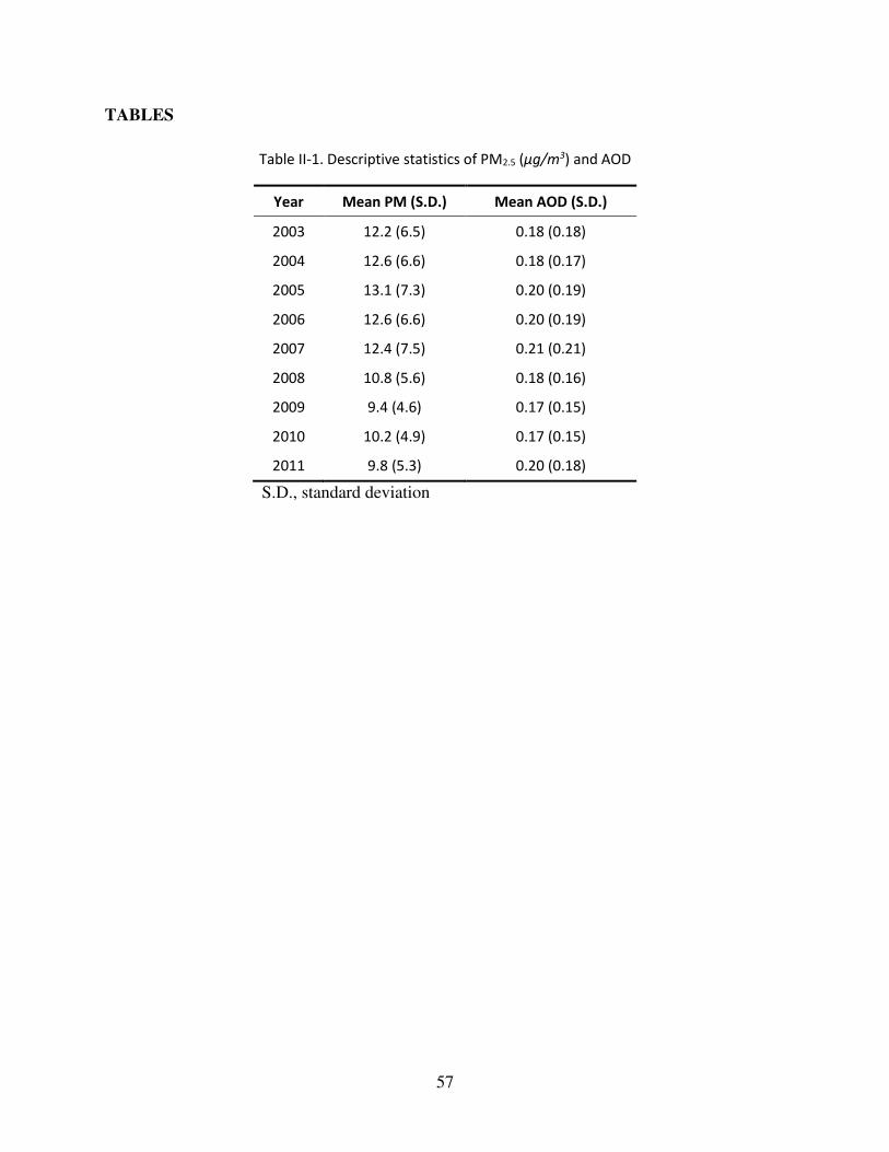
57

TABLES

Table II-1. Descriptive statistics of PM2.5 (ʅŐͬŵ3) and AOD

Year Mean PM (S.D.) Mean AOD (S.D.)

2003 12.2 (6.5) 0.18 (0.18)

2004 12.6 (6.6) 0.18 (0.17)

2005 13.1 (7.3) 0.20 (0.19)

2006 12.6 (6.6) 0.20 (0.19)

2007 12.4 (7.5) 0.21 (0.21)

2008 10.8 (5.6) 0.18 (0.16)

2009 9.4 (4.6) 0.17 (0.15)

2010 10.2 (4.9) 0.17 (0.15)

2011 9.8 (5.3) 0.20 (0.18)

S.D., standard deviation

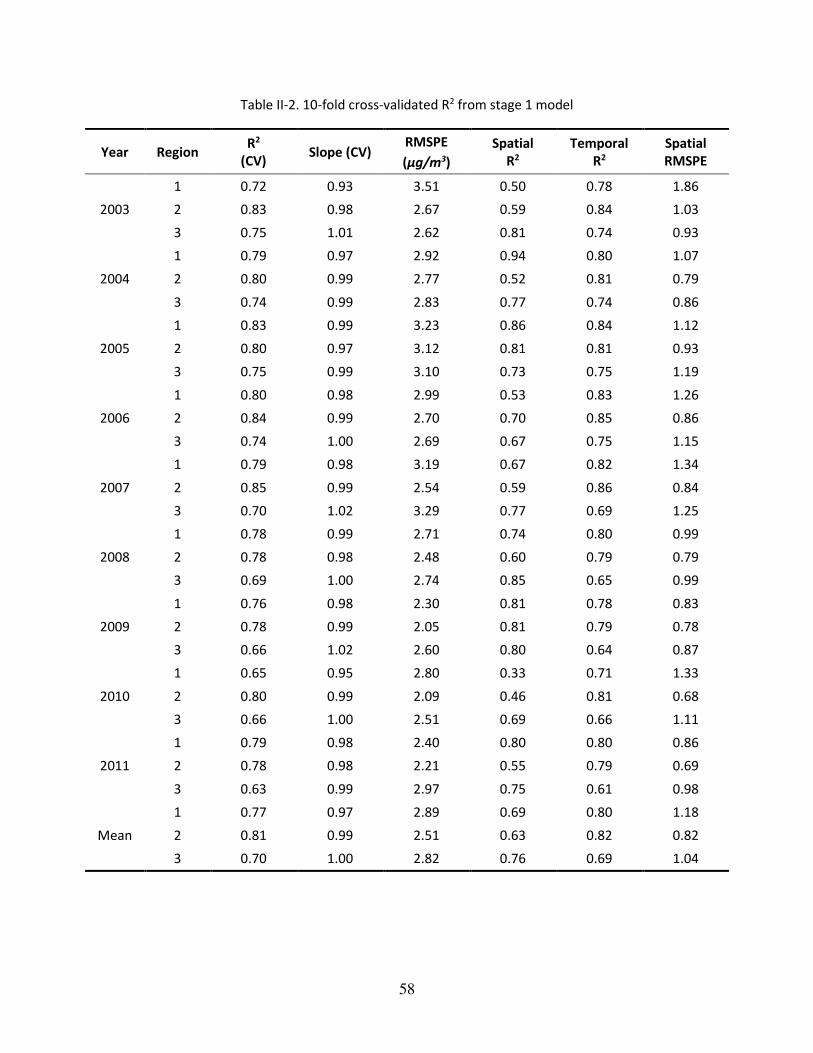
58

Table II-2. 10-fold cross-validated R2 from stage 1 model

Year Region R2

(CV) Slope (CV)

RMSPE

(ʅŐͬŵ3)

Spatial

R2

Temporal

R2

Spatial

RMSPE

2003

1 0.72 0.93 3.51 0.50 0.78 1.86

2 0.83 0.98 2.67 0.59 0.84 1.03

3 0.75 1.01 2.62 0.81 0.74 0.93

2004

1 0.79 0.97 2.92 0.94 0.80 1.07

2 0.80 0.99 2.77 0.52 0.81 0.79

3 0.74 0.99 2.83 0.77 0.74 0.86

2005

1 0.83 0.99 3.23 0.86 0.84 1.12

2 0.80 0.97 3.12 0.81 0.81 0.93

3 0.75 0.99 3.10 0.73 0.75 1.19

2006

1 0.80 0.98 2.99 0.53 0.83 1.26

2 0.84 0.99 2.70 0.70 0.85 0.86

3 0.74 1.00 2.69 0.67 0.75 1.15

2007

1 0.79 0.98 3.19 0.67 0.82 1.34

2 0.85 0.99 2.54 0.59 0.86 0.84

3 0.70 1.02 3.29 0.77 0.69 1.25

2008

1 0.78 0.99 2.71 0.74 0.80 0.99

2 0.78 0.98 2.48 0.60 0.79 0.79

3 0.69 1.00 2.74 0.85 0.65 0.99

2009

1 0.76 0.98 2.30 0.81 0.78 0.83

2 0.78 0.99 2.05 0.81 0.79 0.78

3 0.66 1.02 2.60 0.80 0.64 0.87

2010

1 0.65 0.95 2.80 0.33 0.71 1.33

2 0.80 0.99 2.09 0.46 0.81 0.68

3 0.66 1.00 2.51 0.69 0.66 1.11

2011

1 0.79 0.98 2.40 0.80 0.80 0.86

2 0.78 0.98 2.21 0.55 0.79 0.69

3 0.63 0.99 2.97 0.75 0.61 0.98

Mean

1 0.77 0.97 2.89 0.69 0.80 1.18

2 0.81 0.99 2.51 0.63 0.82 0.82

3 0.70 1.00 2.82 0.76 0.69 1.04

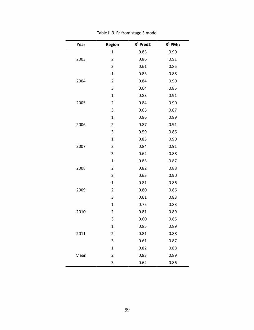
59

Table II-3. R2 from stage 3 model

Year Region R2 Pred2 R2 PM25

2003

1 0.83 0.90

2 0.86 0.91

3 0.61 0.85

2004

1 0.83 0.88

2 0.84 0.90

3 0.64 0.85

2005

1 0.83 0.91

2 0.84 0.90

3 0.65 0.87

2006

1 0.86 0.89

2 0.87 0.91

3 0.59 0.86

2007

1 0.83 0.90

2 0.84 0.91

3 0.62 0.88

2008

1 0.83 0.87

2 0.82 0.88

3 0.65 0.90

2009

1 0.81 0.86

2 0.80 0.86

3 0.61 0.83

2010

1 0.75 0.83

2 0.81 0.89

3 0.60 0.85

2011

1 0.85 0.89

2 0.81 0.88

3 0.61 0.87

Mean

1 0.82 0.88

2 0.83 0.89

3 0.62 0.86

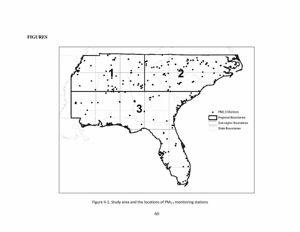
60

FIGURES

Figure II-1. Study area and the locations of PM2.5 monitoring stations

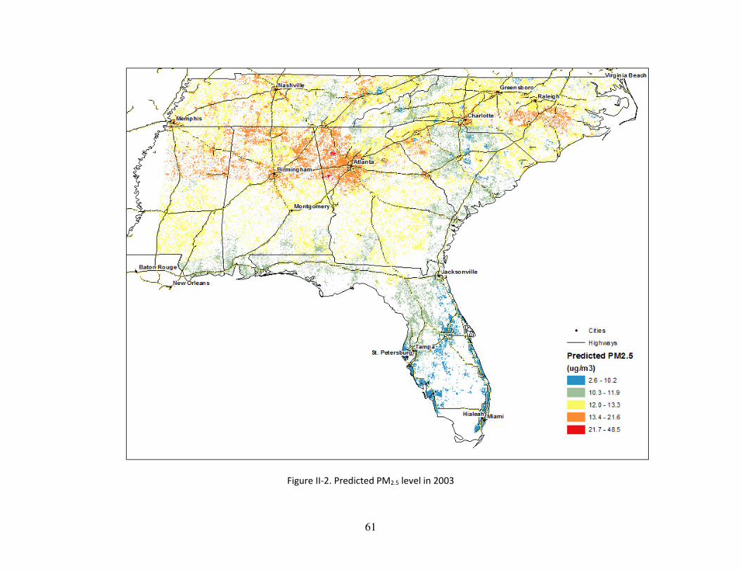
61

Figure II-2. Predicted PM2.5 level in 2003

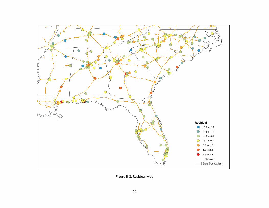
62

Figure II-3. Residual Map

!(

!(

!(

!(

!(

!(

!(

!(!(

!(!(

!( !(!(!(

!(!(

!(

!(!(

!(

!(!(

!(

!(

!( !(!(

!(

!(!(

!(

!(!(!(!(

!(

!(!(!(

!(!(!(!(!(!(!(

!(!(!(

!(

!(

!(

!(

!(!(

!(

!(!(

!( !(

!(

!(!( !(

!(

!(

!(

!(

!(

!(!(

!(!(

!(!(

!(

!(!(

!(!(

!(

!(!(

!(!(!(

!(

!(

!(

!(

!(

!(!(!(

!(

!(!(

!(

!(!(

!(

!(

!(!(!(!(

!(!(!(!(

!(

!(!(!(

!(

!(

!(

!(

!(

!(

!(

!(

!( !(!(!(

!(

!(!(!(

!(

!(!( !(!(!(!(!(

!(

!(!(

!(!(!(!(

!(!(

!(!(!(!(

!(

!(

!(

!(

!(

!(

!(!(

!(

!(!(

!(!(!(

!(

!(

!(

!(

!(

!(!(!(!(!(

!(

!(!(

!(

!(!(!(!(!(!(!(

!(

!(

!(

!(

!(!(!(!(

!(

!(

!(!(!(!(

!(

!(!(!(!(

!(

!(!( !(

!(!(

!(!(

!(!(!(

!(!(!(!(!(!(

!(!(

Residual

!( -2.8 to -1.9

!( -1.8 to -1.1

!( -1.0 to -0.2

!( -0.1 to 0.7

!( 0.8 to 1.5

!( 1.6 to 2.4

!( 2.5 to 3.3

Highways

State Boundaries

63

CHAPTER III

Acute effect of fine particulate matter on mortality in three southeastern

states 2007-2011: statewide analysis

Mihye Lee1, Petros Koutrakis, Brent Coull, Itai Kloog2, Joel Schwartz1,

1Department of Environmental Health, Harvard School of Public Health,

Boston, MA, USA

2Department of Geography and Human Environment, Tel-Aviv University, Israel

64

Dissertation Advisor: Dr. Joel Schwartz Mihye Lee

Acute effect of fine particulate matter on mortality in three southeastern states 2007-2011:

statewide analysis

Abstract

Many studies, both time series and case-crossover analyses, have examined the acute

effects of air pollution on mortality. However, they have generally been limited to larger cities,

because that is where the air pollution monitors are, and have assigned all residents of those cities

the same exposure, introducing exposure error. We have developed a spatiotemporal model to

predict daily PM2.5 level at a 1 km×1km resolution for the Southeastern United States between

2003 through 2011. We have also obtained zip-code level mortality data in three of those states:

North Carolina, South Carolina, and Georgia between 2007 and 2011. This allows us to examine

the acute effect of PM2.5 on mortality in the entire population using finer resolution exposure.

We acquired mortality data from the departments of public health in the three states.

Modeled PM2.5 level from our prediction model were assigned to the zip code of residence of each

decedent. We used a case-crossover study design rather than a time series because it allowed easier

examination of effect size modification. We examined modification by age, sex, race, education,

the primary cause of death, and residence in urban or rural areas. We also compared results based

on our modeled PM2.5 with the one from using the nearest monitor.

848,270 non-accidental death records were analyzed and we found each 10 たg/m3 increase

in PM2.5 (mean lag0 and lag1) was associated with a 1.56 % (1.19, 1.94) increase in daily deaths.

65

Cause-specific analyses revealed that cardiovascular disease (2.32 %, 1.57-3.07) and specifically

congestive heart failure (3.64 %, 1.35-5.99) showed the highest effect estimate. Blacks (2.19 %,

1.43-2.96) and persons with education ≤ 8 yr (3.13 %, 2.08-4.19) were the most vulnerable

populations. Compared to monitoring measurement, our results showed more power and suggested

that the PM2.5 effects on rural populations have been underestimated due to selection bias and

information bias.

We have demonstrated that our AOD-based exposure models can be successfully applied

to epidemiologic studies investigating the acute effects of PM2.5. This will add a new study

population in rural areas, and by doing this, the result from those analyses will be generalizable to

a larger population.

66

INTRODUCTION

Numerous epidemiologic studies have reported a positive relationship between acute

exposures to fine particles (particles less than 2.5 micrometers in diameter, PM2.5) and mortality

ranging from all-cause deaths to respiratory or cardiovascular death (Samet et al. 2000, 1742-1749;

Wichmann et al. 2000, 5-86; discussion 87-94; Mar et al. 2005, 311-320; Boldo et al. 2006, 449-

458; Ostro, Broadwin, and Lipsett 2000, 412-419; Franklin, Zeka, and Schwartz 2006, 279-287;

Ruchirawat et al. 2007, 200-209). PM2.5 is believed to increase mortality by producing

inflammation and oxidative stress (Risom, Moller, and Loft 2005, 119-137), in part because its

small size allows it to penetrate into the alveoli and be retained in the lung parenchyma (Dockery

2009, 257-263). Toxicological research have shown that the components of PM2.5 such as metals,

sulfate, nitrate, or organic compounds also elicit reactive oxygen species (ROS), inflammatory

injury, oxidative DNA damage, and other biological effects (Valavanidis, Fiotakis, and

Vlachogianni 2008, 339-362).

Traditionally, PM2.5 measurements from ground monitoring stations centrally located in

the study domain have been used as surrogates for individual-level exposures to PM2.5. Ecological

exposure assignment is more subject to biases than individual-level exposure measurement, and

the increased measurement error generally makes the risk estimates attenuated (Brenner et al.

1992, 85-95) and results in less statistical power (Greenland 1992, 1209-1223). The use of the

existing monitoring stations imposes temporal limitations as well as spatial. Many monitors in the

U.S. operate only every third or even sixth day.

As a result, a majority of studies are done in cities or urban areas close to the location of

those monitors. Restriction in study population imposes a problem in generalizability of those

epidemiologic studies.

67

However, the characteristics of rural populations are different from urban populations

including factors such as education, housing, and the accessibility to health care facilities, and this

may lead to a different response to environmental stimuli. Therefore, there have been a lot of

uncertainties about acute PM2.5 effects outside of large cities.

Recently, we have developed a spatiotemporal model to predict daily PM2.5 level at a 1

km×1km resolution for the Southeastern United States between 2003 through 2011. It allowed us

to estimate spatially resolved PM2.5 on a daily basis throughout the 7 states located in the

Southeastern U.S: North Carolina, South Carolina, Georgia, Tennessee, Alabama, Mississippi, and

Florida. We have also obtained zip-code level mortality data in three of those states: North

Carolina, South Carolina, and Georgia between 2007 and 2011. Therefore, we use our model

generated predictions to study the acute effect of PM2.5 on mortality in the entire population of

North Carolina, South Carolina, and Georgia between 2007 and 2011.

DATA AND METHODS

Outcome

We acquired mortality data from the departments of public health in Georgia, North

Carolina, and South Carolina. Data was available between 2007 through 2011. The data variables

include the date of death, age, sex, race, education, primary cause of death in ICD-code 10th

version, and residential zip code. We restricted our analyses to deaths from internal causes by

excluding ICD codes V01 through Y98. Specific causes were derived from the ICD code for the

underlying cause of death: respiratory disease (ICD codes J00 through J99), cardiovascular disease

(ICD codes I01 through I52), and stroke (ICD codes I60 through J69).

68

As a result, we used 848,270 non-accidental deaths occurring in the study area from 2007

through 2011. Mortality data were unidentifiable, therefore, our research was exempted by the

Harvard School of Public Health’s Human Subjects Committee.

Exposure

Daily PM2.5 exposures were assessed using our recently developed prediction models that

incorporate satellite AOD (Aerosol Optical Depth) data for the years 2007–2011 in the

Southeastern United States at a 1 × 1 km resolution. The prediction dataset covers virtually the

entire areas of North Carolina, South Carolina, Georgia, Tennessee, Alabama, Mississippi, and

Florida. We used ground PM2.5 measurements from 277 monitoring sites from the Environmental

Protection Agency (EPA) and Interagency Monitoring of Protected Visual Environments

(IMPROVE) monitoring networks to calibrate our model. Our predictors were AOD data from the

Moderate Resolution Imaging Spectroradiometer (MODIS) on the Aqua satellite (at a 1km

resolution), land use terms (elevation, distance to major roads, percent of open space, point

emissions and area emissions) and meteorological variables (temperature, wind speed, relative

humidity and visibility). Firstly, we calibrated the AOD grid-level observations to the PM2.5

monitoring data collected within 1 km of a PM2.5 measurement using a mixed model for observed

PM2.5 (containing both fixed and day-specific random effects), the AOD slopes with additional

spatiotemporal predictors. In doing so, we applied inverse probability weights (IPW) to the first

stage model to adjust for the non-random missingness of AOD. To accommodate the fact that the

PM-AOD calibration factors can vary spatially between large regions, we divided the Southeastern

area into 3 regions and each region has its sub-regions. The intercept, AOD, and temperature

random effects in the model are nested within regions of the study. In stage 2 of the model, we

69

simply predicted PM2.5 concentrations to grid cells without monitors using the model fit. We also

predicted for the location- days that were missing AOD observations using regressions against

nearby monitors and interpolation with a smoothing function. Specifically, for each region in the

Southeast, we used the PM2.5 predictions for the days when AOD was not missing, and estimated

a smooth function of latitude and longitude with a random intercept for each cell and a slope for

the mean of PM2.5 monitors within 100 km of the grid cell on that day. The results of this model

were used to estimate the PM2.5 for gridcell-days where AOD was missing. To validate our model,

we performed 10-fold cross-validation and chose our model to maximize cross-validated R2. As a

result, we obtained reasonable and reliable PM2.5 predictions for the study area (mean cross-

validated R2 of 0.77, 81, 0.70 for region 1, 2, 3, respectively) with modest daily predictions errors

(RMSPE -Root of the mean squared prediction errors = 2.89, 2.51, 2.82 たg/m3 for region 1, 2, 3,

respectively). Among the regions, Region 2 displayed best fit, and includes North Carolina, South

Carolina, and part of Georgia. Furthermore, the slopes between observed vs. predicted were close

to 1, indicating no bias. PM2.5 exposure estimates were generated by our prediction models. For

more detailed information on the prediction model, refer to Lee et al.

For this study, the daily predictions of PM2.5 at a 1 km2 resolution were aggregated into the

zip code level. Then they were assigned to the zip code of each descendent on each day.

Ground particulate matter measurements

To compare the result from modeled PM2.5 with the one from measured PM2.5, we used the

monitored PM2.5 mass concentration from the EPA and IMPROVE monitors described previously.

We assigned the resident zip code of the deceased to the nearest monitor. 62,467 observations from

96 PM2.5 monitoring stations which operated in the three states between 2007 and 2011 were used.

70

Covariates

We downloaded daily temperature data from the Climate Data Online website hosted by

NOAA’s National Data Centers (NNDC) at The National Oceanic and Atmospheric

Administration (NOAA) National Climate Data Center (NCDC, 2010). To fully exploit the

temperature data, we selected stations regardless of the operation period. Therefore, the stations

that had only partially run from 2007 to 2011 were also used. As a result, 26 stations were used.

Grid cells were matched to the closest weather station on a specific day with available

meteorological variables (24-hour means).

To classify zip codes into urban versus rural areas, we downloaded the 2004 ZIP Rural-

Urban Commuting Area Codes (RUCAs) from the website of the WWAMI (WWAMI states:

Washington, Wyoming, Alaska, Montana, and Idaho) Rural Health Research Center RHRC.

RUCAs are a census tract-based classification scheme to characterize all of the nation's Census

tracts regarding their rural and urban status. It was based on 2000 Census work commuting

information, and Census Bureau defined Urbanized Areas (cities of 50,000 and greater population)

and Urban Clusters (cities/towns with populations from 2,500 through 49,999) and a ZIP Code

RUCA approximation has been developed. We utilized that data to classify zip codes in the study

area as being urban or rural. RUCA version 2 was used. When the RUCA code is 1.0 or 1.1 which

stands for the metropolitan area core, the corresponding zip code area was defined as an urban

area. The spatial distribution of urbaneness by zip code is given by Figure III-1.

71

Statistical analyses

Zip code-specific deaths were matched with our exposure estimates for each grid cell. For

monitoring data, we assigned the closest monitoring stations on a specific day. Since many

monitoring stations operate on every third or sixth day, we found the next closest monitoring

station, if the closest monitoring station didn’t run on a specific day.

We used a case-crossover design (Maclure 1991, 144-153), which is a variant of the

matched case-control design to study the effects of acute exposures on the acute outcome without

carry-over effect. In this design, each case subject (a decedent) serves as his or her own control on

days when no event (death) occurs. Since each subject serves as his or her own control, it provides

perfect matching on all subject characteristics that do not vary over time. To avoid seasonal

confounding, control days are only chosen within the same month of the same year that death

occurred. Control days are chosen bi-directionally and we chose every third day from the case day

in that month to reduce serial correlation in the exposure variable, given that in the US weather

fronts generally pass through a location every 3–4 days (Medina-Ramon and Schwartz 2007, 827-

833).

We defined the relevant exposure time window as the mean exposure on the day of and

day before the decedent’s death. Temperature was chosen as a potential confounder. Specifically,

a conditional logistic regression was fitted as follows,

logit (pi) = 紅待沈 + 紅怠鶏堅結穴鶏警態┻泰日乳 髪 紅態劇結兼喧沈珍 + 紅戴Tuesday + 橋 + 紅腿Sunday,

where 鶏堅結穴鶏警態┻泰日乳 is the predicted two day mean PM2.5 level in zip code i on day j, 劇結兼喧沈珍 is the temperature for zip code i on day j, and the remaining are the indicator variables for

day of the week.

72

For stratified analysis, we performed separate analyses to generate the effect estimate but

used the interaction term with the exposure and the effect modifier to test for significant

modification. For those sub-region analyses, we used the same exposure window as in the main

analysis. Various stratified analyses were conducted: we examined effect modification by age, sex,

race, education, and the primary cause of death. We also conducted analyses to compare the results

that used modeled PM2.5 with those using actual PM2.5 measurement data.

The data analysis for this paper was generated using the PROC PHREG procedure in Base

SAS software, version 9.3 of the SAS system for windows (Copyright © 2014 SAS Institute Inc.,

Cary, NC, USA).

RESULTS

Figure III-1 shows the study area. Zip codes are divided by being urban or rural. Main

cities in the study areas were Atlanta (GA), Charlotte (NC), Raleigh (NC), and Columbia (SC).

Most of the PM2.5 monitors operated in urban areas. Figure III-2 presents one of the examples from

our PM2.5 prediction models, which is aggregated into a zip code level. It shows the spatial

distribution of the average of modeled PM2.5 in the study area in 2011 by zip code. The spatial

distribution of PM2.5 was relatively high in Georgia among three states and urban areas showed

higher PM2.5 level compared to the surrounding rural areas.

We used 848,270 non-accidental death records in three states of North Carolina, South

Carolina, and Georgia between 2007 and 2011 (Table III-1). By state, 42% of the total record was

collected from North Carolina, 37% of data from Georgia, and 21% was from South Carolina. The

average age of the decedents was 73 years old with a standard deviation of 17 years. Therefore,

73

most of the decedents were aged over 65 (71 %) and about the half of the deceased died at 75 or

over. The sex ratio was almost 1:1 with a slight excess of females (52 %). By race, whites

accounted for 75 % of deaths, blacks for 24 %, and other races for 1 %. The percentage of whites

was highest in North Carolina (78 %). For education level, less than high school education (years

less than 12 years) occurred with the highest frequency (27 %). However 24 % of the education

records were missing and most of that originated from data collected from Georgia (63% of

Georgia records). 53 % of the population resided in urban areas and the proportion was highest in

Georgia (59%). It is worth noting that the 4,339 (0.5 %) missing data on being urban or not includes

true missing data as well as those with a residential zip code outside the study area.

Table III-1 also shows a summary of the modeled PM2.5 level for rural/urban areas and

temperature. The average PM2.5 level was 11.1 たg/m3 (S.D.=4.4 たg/m3) from 2007 through 2011

and the average PM2.5 in Georgia was slightly higher than the other states.

Table III-2 presents the estimated percent increase in mortality for a 10 たg/m3 increase in

PM2.5 by lag period and its comparison with the results from measurement data. For all non-

accidental deaths, we found a 1.56 % increase in mortality (95% CI = 1.19 to 1.94). Compared to

the result from our prediction model, the estimate from the existing monitoring stations showed a

lower effect estimate, which was 1.21 % increase. The mean distance to the assigned monitors was

around 55 km. It is worth noting the distances were different between lag 0 and lag 1, because

many monitoring stations don’t operate on a daily basis.

We conducted various sub-region analyses (Figure III-3). There was no significant effect

modification by age, sex or race. However, we found that black population showed substantially

higher risk (2.19%, 95% CI=1.43-2.96) than white population (1.40 %). While not significant, a

50% difference in effect size is noteworthy, and the significance may have been affected by the

74

small percentage of deaths that were blacks. For education level, the region less than 8 years of

education showed more than double the risk (3.13%) compared to the more educated regions (1.43

%), and that difference was marginally significant.

The impact of PM2.5 on CVD and CHF death rates was larger than for all natural causes;

we found a 2.32 percent increase (95% CI =1.57 to 3.07) and a 3.64 % (1.35, 5.99) respectively.

In contrast, the impact on deaths from MI (1.12 %) and stroke (0.55 %) was lower. We did not see

significant associations with pulmonary deaths, perhaps because of small numbers.

We found differences (albeit not significant based on the p-value of the interaction term)

in the PM2.5 associations with mortality between people living in urban areas and those in rural

areas and those results were reversed between modeled PM2.5 and measured PM2.5 (Figure III-4).

Rural areas showed the higher risk for mortality (1.86 %; 1.75, 1.98) than the urban areas (1.38 %;

1.28, 1.47) in our analyses. Conversely, results based on the existing monitoring stations, showed

a higher increase in mortality in urban areas (1.43 %; 1.36, 1.50) than rural areas (0.96 %; 0.88,

1.03).

DISCUSSION

In this paper we examine associations between PM2.5 exposures generated by our

prediction model and increased mortality in the three states of Georgia, North Carolina, and South

Carolina between 2007 through 2011.

Compared to the effect estimate from our modeled PM2.5, monitor-based estimates tended

to be attenuated, and have wider confidence intervals. The use of the modeled PM2.5 levels enabled

us to investigate the entire region, with more power to conduct stratified analyses. We found

75

differences in effect size by race and education level, with blacks and less educated people having

higher risk. While some studies using central monitoring sites have identified such effect

modification before, the nature of the study design made it impossible to determine whether these

effects were due to differential exposure or differential response. Our results, using 1km resolution

exposure estimates strongly suggest that in addition to any differential exposure, there is

differential response. This makes particulate air pollution a key environmental justice issue, since

it is ubiquitous, and associated with more harm than most environmental exposures. Whether these

differences relate to psychosocial stress, housing, or other factors needs further investigation.

In the stratified analyses for the primary cause of death, CVD and CHF exhibited the

highest increase in mortality in response to PM2.5. Other causes were not significant, likely due to

the very small number of observations (Figure III-3).

We also found differences in the PM2.5 associations between people living in rural areas

and urban areas. Interestingly, the effects of acute PM2.5 exposure appeared stronger in rural areas

than urban areas. Kloog et al. (Kloog et al. 2014, e88578) reported results consistent with this in

his paper where he used a similar model for PM2.5 in the mid-Atlantic region of U.S. In contrast,

using the nearest monitor we failed to find this result. Since that exposure overall produces lower

effect size estimates, a result consistent with larger exposure error, the difference using this

exposure likely reflects the higher measurement error in exposure in rural areas, because most

residents live further from a monitor.

Another consequence of this finding is that the acute effects of particulate matter may have

been underestimated because an important part of the population was excluded from most prior

epidemiologic studies due to the lack of monitoring sites.

76

A possible explanation for the higher risk in rural areas can be sought in the socioeconomic

characteristics of rural populations who tend to be in low income and education level compared to

the population in urban areas (Kloog et al. 2014, e88578). Alternatively, these differences may be

related to differences in the amount of outdoor time such as farmers, accessibility to hospitals or

the prevalence of smoking.

We don’t expect any problem in the exposure history, since we evaluated acute exposure

with the history of exposure only within 1 previous day and used the zip codes for residence.

Therefore, discrepancy in the record and the actual exposure is very low.

There are still limitations in our study. The resident location of the deceased was in an

aggregated form of zip codes, not individual addresses which were not available due to privacy

and confidentiality issues. This ecological attribute in exposure measurement still lends more

measurement error than individual-level studies. With 1 km resolution exposure day, once we

obtain the street-level address from study subjects, our research question will be better served. Yet,

considering the area of zip code is much smaller than a city or a county, the magnitude of such

error seems much smaller than the existing studies that used the sparse network of monitoring

stations.

We also expect further improvements of the prediction. With an advent of finer satellite

remote sensing and processing algorithms, we will be able to produce more reliable and accurate

predictions of PM2.5.

The same issue also exists for the covariate, temperature. Temperature was controlled as a

possible confounder and its measurement was not based on the individual-level as well. The

residual confounding in temperature is expected.

77

To the best of our knowledge, this is the first study that included the entire population in

the three states in the Southeastern U.S. to assess the relationship between short-term PM2.5

exposures and mortality.

In conclusion, our findings indicate that increased mortality especially for CVD and CHF

were associated with PM2.5 exposures. In addition, we have demonstrated that our AOD-based

exposure models can be successfully applied to epidemiologic studies investigating the acute

effects of PM2.5. This has been possible because these models make it possible to estimate

spatially-resolved PM2.5 exposures for specific zip codes on a daily basis. This will add a new

study population in rural areas, and in doing so, the result from those analyses will be more

generalizable to other populations and areas.

78

REFERENCES

1. Samet JM, Dominici F, Curriero FC, Coursac I, Zeger SL. Fine particulate air pollution and mortality

in 20 U.S. cities, 1987-1994. N Engl J Med. 2000;343(24):1742-1749. doi:

10.1056/NEJM200012143432401 [doi].

2. Wichmann HE, Spix C, Tuch T, et al. Daily mortality and fine and ultrafine particles in erfurt, germany

part I: Role of particle number and particle mass. Res Rep Health Eff Inst. 2000(98):5-86; discussion

87-94.

3. Mar TF, Ito K, Koenig JQ, et al. PM source apportionment and health effects. 3. investigation of inter-

method variations in associations between estimated source contributions of PM2.5 and daily mortality

in phoenix, AZ. J Expos Sci Environ Epidemiol. 2005;16(4):311-320.

4. Boldo E, Medina S, Le Tertre A, et al. Apheis: Health impact assessment of long-term exposure to PM2.5

in 23 european cities. Eur J Epidemiol. 2006;21(6):449-458. doi: 10.1007/s10654-006-9014-0.

5. Ostro BD, Broadwin R, Lipsett MJ. Coarse and fine particles and daily mortality in the coachella valley,

california: A follow-up study. J Expo Anal Environ Epidemiol. 2000;10(5):412-419. doi:

10.1038/sj.jea.7500094.

6. Franklin M, Zeka A, Schwartz J. Association between PM2.5 and all-cause and specific-cause mortality

in 27 US communities. J Expos Sci Environ Epidemiol. 2006;17(3):279-287.

7. Ruchirawat M, Settachan D, Navasumrit P, Tuntawiroon J, Autrup H. Assessment of potential cancer

risk in children exposed to urban air pollution in bangkok, thailand. Toxicol Lett. 2007;168(3):200-209.

doi: S0378-4274(06)01323-3 [pii].

8. Risom L, Moller P, Loft S. Oxidative stress-induced DNA damage by particulate air pollution. Mutat

Res. 2005;592(1-2):119-137. doi: S0027-5107(05)00246-0 [pii].

79

9. Dockery DW. Health effects of particulate air pollution. Ann Epidemiol. 2009;19(4):257-263. doi:

10.1016/j.annepidem.2009.01.018 [doi].

10. Valavanidis A, Fiotakis K, Vlachogianni T. Airborne particulate matter and human health:

Toxicological assessment and importance of size and composition of particles for oxidative damage and

carcinogenic mechanisms. J Environ Sci Health C Environ Carcinog Ecotoxicol Rev. 2008;26(4):339-

362. doi: 10.1080/10590500802494538 [doi].

11. Brenner H, Savitz DA, Jockel KH, Greenland S. Effects of nondifferential exposure misclassification

in ecologic studies. Am J Epidemiol. 1992;135(1):85-95.

12. Greenland S. Divergent biases in ecologic and individual-level studies. Stat Med. 1992;11(9):1209-

1223.

13. Maclure M. The case-crossover design: A method for studying transient effects on the risk of acute

events. Am J Epidemiol. 1991;133(2):144-153.

14. Medina-Ramon M, Schwartz J. Temperature, temperature extremes, and mortality: A study of

acclimatisation and effect modification in 50 US cities. Occup Environ Med. 2007;64(12):827-833. doi:

10.1136/oem.2007.033175 [doi].

15. Schwartz J, Coull B, Laden F, Ryan L. The effect of dose and timing of dose on the association between

airborne particles and survival. Environ Health Perspect. 2008;116(1):64-69. doi: 10.1289/ehp.9955

[doi].

16. Lepeule J, Laden F, Dockery D, Schwartz J. Chronic exposure to fine particles and mortality: An

extended follow-up of the harvard six cities study from 1974 to 2009. Environ Health Perspect.

2012;120(7):965-970. doi: 10.1289/ehp.1104660 [doi].

80

17. Kloog I, Nordio F, Zanobetti A, Coull BA, Koutrakis P, Schwartz JD. Short term effects of particle

exposure on hospital admissions in the mid-atlantic states: A population estimate. PLoS One.

2014;9(2):e88578. doi: 10.1371/journal.pone.0088578 [doi].

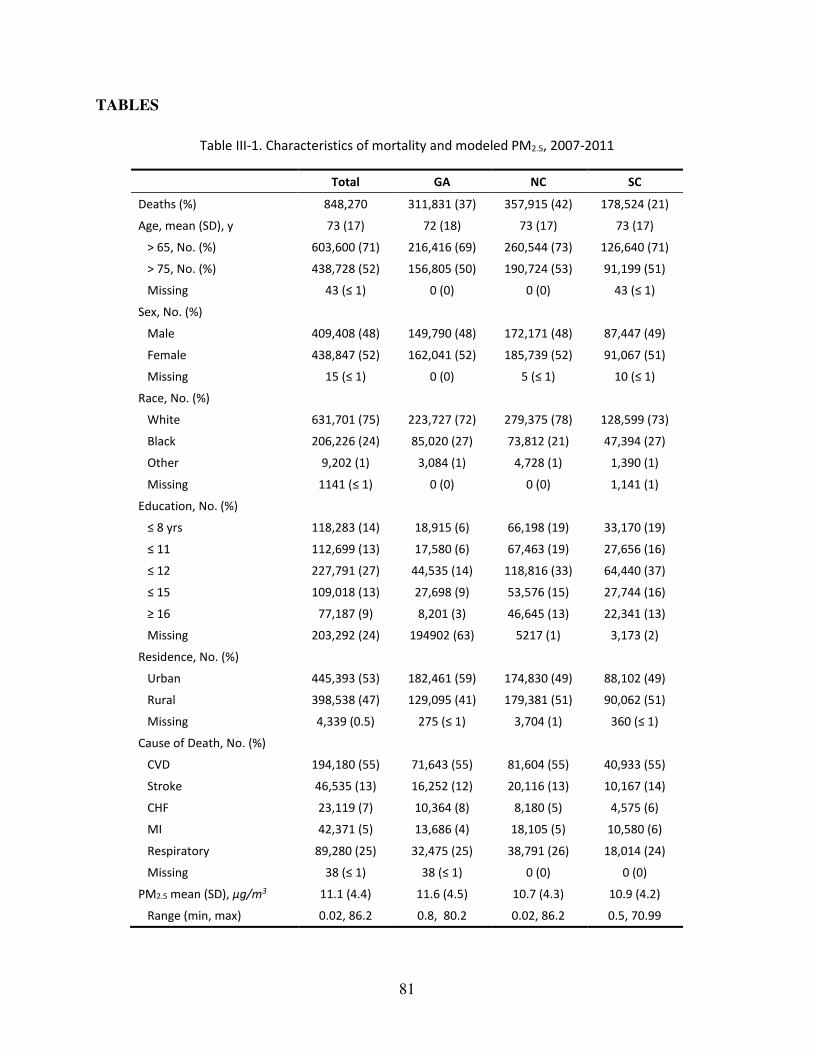
81

TABLES

Table III-1. Characteristics of mortality and modeled PM2.5, 2007-2011

Total GA NC SC

Deaths (%) 848,270 311,831 (37) 357,915 (42) 178,524 (21)

Age, mean (SD), y 73 (17) 72 (18) 73 (17) 73 (17)

> 65, No. (%) 603,600 (71) 216,416 (69) 260,544 (73) 126,640 (71)

> 75, No. (%) 438,728 (52) 156,805 (50) 190,724 (53) 91,199 (51)

Missing ヴン ふг ヱぶ 0 (0) 0 (0) ヴン ふг ヱぶ

Sex, No. (%)

Male 409,408 (48) 149,790 (48) 172,171 (48) 87,447 (49)

Female 438,847 (52) 162,041 (52) 185,739 (52) 91,067 (51)

Missing ヱヵ ふг ヱぶ 0 (0) ヵ ふг ヱぶ ヱヰ ふг ヱぶ

Race, No. (%)

White 631,701 (75) 223,727 (72) 279,375 (78) 128,599 (73)

Black 206,226 (24) 85,020 (27) 73,812 (21) 47,394 (27)

Other 9,202 (1) 3,084 (1) 4,728 (1) 1,390 (1)

Missing ヱヱヴヱ ふг ヱぶ 0 (0) 0 (0) 1,141 (1)

Education, No. (%)

г Β ┞ヴゲ 118,283 (14) 18,915 (6) 66,198 (19) 33,170 (19)

г ヱヱ 112,699 (13) 17,580 (6) 67,463 (19) 27,656 (16)

г ヱヲ 227,791 (27) 44,535 (14) 118,816 (33) 64,440 (37)

г ヱヵ 109,018 (13) 27,698 (9) 53,576 (15) 27,744 (16)

д ヱヶ 77,187 (9) 8,201 (3) 46,645 (13) 22,341 (13)

Missing 203,292 (24) 194902 (63) 5217 (1) 3,173 (2)

Residence, No. (%)

Urban 445,393 (53) 182,461 (59) 174,830 (49) 88,102 (49)

Rural 398,538 (47) 129,095 (41) 179,381 (51) 90,062 (51)

Missing 4,339 (0.5) ヲΑヵ ふг ヱぶ 3,704 (1) ンヶヰ ふг ヱぶ

Cause of Death, No. (%)

CVD 194,180 (55) 71,643 (55) 81,604 (55) 40,933 (55)

Stroke 46,535 (13) 16,252 (12) 20,116 (13) 10,167 (14)

CHF 23,119 (7) 10,364 (8) 8,180 (5) 4,575 (6)

MI 42,371 (5) 13,686 (4) 18,105 (5) 10,580 (6)

Respiratory 89,280 (25) 32,475 (25) 38,791 (26) 18,014 (24)

Missing ンΒ ふг ヱぶ ンΒ ふг ヱぶ 0 (0) 0 (0)

PM2.5 mean (SD), ʅŐͬŵ3 11.1 (4.4) 11.6 (4.5) 10.7 (4.3) 10.9 (4.2)

Range (min, max) 0.02, 86.2 0.8, 80.2 0.02, 86.2 0.5, 70.99

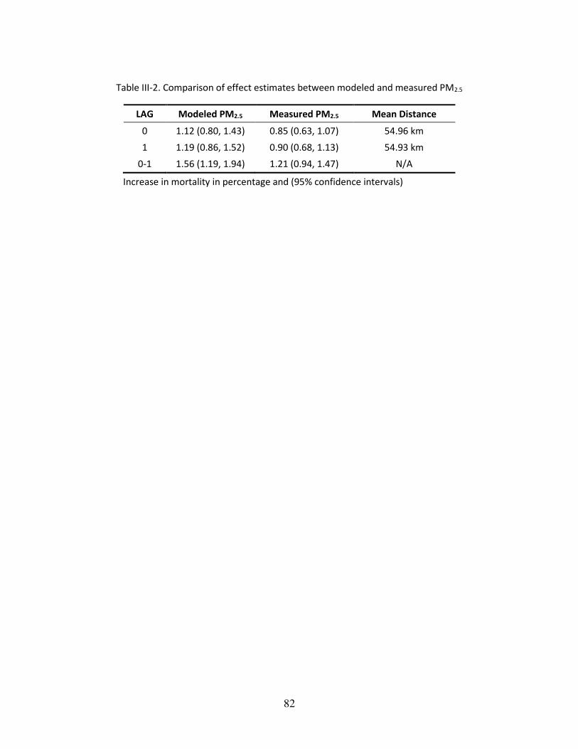
82

Table III-2. Comparison of effect estimates between modeled and measured PM2.5

LAG Modeled PM2.5 Measured PM2.5 Mean Distance

0 1.12 (0.80, 1.43) 0.85 (0.63, 1.07) 54.96 km

1 1.19 (0.86, 1.52) 0.90 (0.68, 1.13) 54.93 km

0-1 1.56 (1.19, 1.94) 1.21 (0.94, 1.47) N/A

Increase in mortality in percentage and (95% confidence intervals)

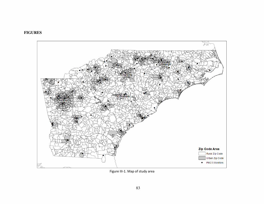
83

FIGURES

Figure III-1. Map of study area

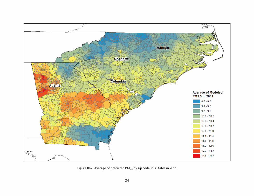
84

Figure III-2. Average of predicted PM2.5 by zip code in 3 States in 2011

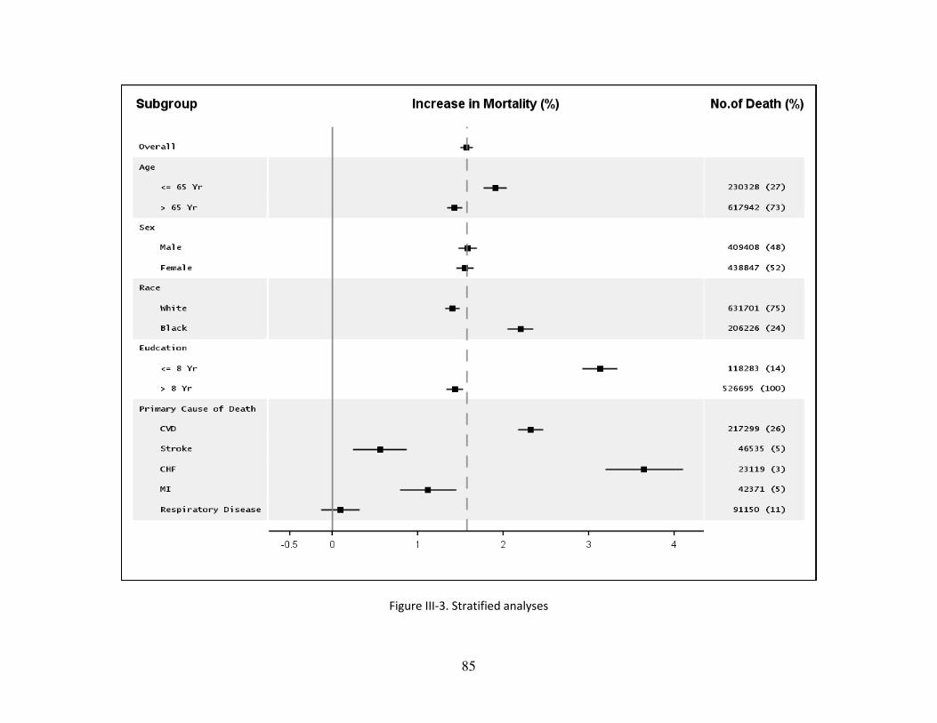
85

Figure III-3. Stratified analyses

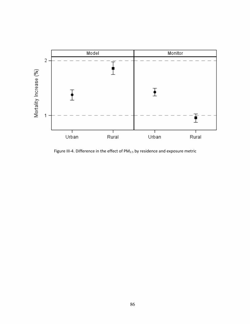
86

Figure III-4. Difference in the effect of PM2.5 by residence and exposure metric

87

CONCLUSION

In our first paper, we found that the effects of a given temperature on mortality vary

spatially and temporally based on how unusual it is for that time and location. This suggests

changes in variability of temperature may be more important for health as climate changes than

changes of mean temperature. More emphasis should be placed on warnings targeted to early

heat/cold temperature for the season or month rather than focusing only on the extremes.

In our second topic, we have demonstrated that the use satellite imagery and other land use

variables with a mixed-effect model produces reliable predictions of daily PM2.5 for the extensive

area of the southeastern United States. By incorporating land use terms and spatial smoothing, our

models perform much better than previous studies. Therefore, our model results can be used in

various epidemiological studies investigating the effects of PM2.5 allowing one to assess both acute

and chronic exposures with the implication of a new application. Our model results will extend the

existing studies on PM2.5 mainly targeted only for urban areas tied to the lack of monitors into new

areas which used not to be studied such as rural areas.

In our third topic, our findings indicate that increased mortality especially for CVD and

CHF were associated with PM2.5 exposures. In addition, we have demonstrated that our AOD-

based exposure models can be successfully applied to epidemiologic studies investigating the acute

effects of PM2.5. This will add a new study population in rural area, and by doing this, the result

from those analyses will be given more generalizability of the conclusion.