Embed Size (px)
Citation preview
THE EFFECT OF AMBIENT AIR AND WATER TEMPERATURE ON POWER PLANT EFFICIENCY
by
Jesse Colman
APR 26, 2013
____________________________ Dr. Lincoln Pratson, Advisor
April 2013
Abstract
The performance of thermoelectric generators depends on a variety of factors, many of which are
meticulously controlled through generator design or operational management. However, there are
environmental factors that affect operations which cannot be controlled directly, such as air
temperature and water temperature. Recent studies have suggested that a warming climate will have a
significant impact on cooling water availability for generators, arising in part from cooling water
regulations designed to protect aquatic ecosystems. Other work has shown the effect of either air or
water temperature on the efficiency of specific generating technologies. The physical relationships
between ambient temperatures, combustion, and cooling processes are well understood, but the
implications of these relationships for real-time plant efficiency across power generating technologies
have not been fully explored in the literature. This study develops empirical estimates for the impact of
air temperature and water temperature on the efficiency of coal- and natural gas-fired power plants
with once-through and recirculating cooling systems.
Using USGS and NOAA air and water temperature data and EPA records of power plant fuel
consumption and power output, this master’s project quantifies the impact of air and water
temperature on power plant efficiency. Regression models developed here indicate that a 1° C increase
in air temperature is correlated with a 0.01 percentage point decrease in plant efficiency and a 1° C
increase in water temperature is correlated with a 0.02 percentage point decrease in plant efficiency,
though these vary for by generating technology and cooling system type. These impacts are substantially
smaller in magnitude than analogous effects quantified in previous studies.
Contents I. Introduction ........................................................................................................................................ 1
II. Relationships between Ambient Temperatures and Efficiency ........................................................... 4
Air Temperature and Efficiency .............................................................................................................. 4
Water Temperature and Efficiency ......................................................................................................... 5
III. Data Collection and Selection ......................................................................................................... 5
Power Plant Data and Record Selection .................................................................................................. 5
Water Temperature Data ........................................................................................................................ 7
Air Temperature and Dew Point Data ..................................................................................................... 8
IV. Methods .......................................................................................................................................... 9
Regression modeling ............................................................................................................................... 9
Modeling Using the IECM ..................................................................................................................... 12
V. Results............................................................................................................................................... 13
Regression Modeling ............................................................................................................................ 13
IECM Model .......................................................................................................................................... 17
VI. Discussiom .................................................................................................................................... 20
Comparing Regression modeling and IECM results ............................................................................... 20
Explanation of insignificant environmental variables ........................................................................... 21
Comparison with previous studies ........................................................................................................ 23
Relevance of results .............................................................................................................................. 24
VII. Conclusion ..................................................................................................................................... 25
References ................................................................................................................................................ 27
Appendix ................................................................................................................................................... 29
1
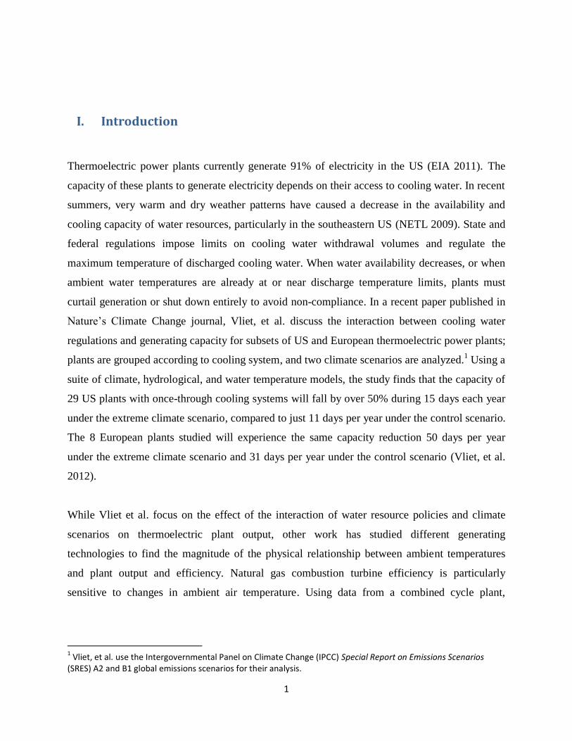
I. Introduction
Thermoelectric power plants currently generate 91% of electricity in the US (EIA 2011). The
capacity of these plants to generate electricity depends on their access to cooling water. In recent
summers, very warm and dry weather patterns have caused a decrease in the availability and
cooling capacity of water resources, particularly in the southeastern US (NETL 2009). State and
federal regulations impose limits on cooling water withdrawal volumes and regulate the
maximum temperature of discharged cooling water. When water availability decreases, or when
ambient water temperatures are already at or near discharge temperature limits, plants must
curtail generation or shut down entirely to avoid non-compliance. In a recent paper published in
Nature’s Climate Change journal, Vliet, et al. discuss the interaction between cooling water
regulations and generating capacity for subsets of US and European thermoelectric power plants;
plants are grouped according to cooling system, and two climate scenarios are analyzed.1 Using a
suite of climate, hydrological, and water temperature models, the study finds that the capacity of
29 US plants with once-through cooling systems will fall by over 50% during 15 days each year
under the extreme climate scenario, compared to just 11 days per year under the control scenario.
The 8 European plants studied will experience the same capacity reduction 50 days per year
under the extreme climate scenario and 31 days per year under the control scenario (Vliet, et al.
2012).
While Vliet et al. focus on the effect of the interaction of water resource policies and climate
scenarios on thermoelectric plant output, other work has studied different generating
technologies to find the magnitude of the physical relationship between ambient temperatures
and plant output and efficiency. Natural gas combustion turbine efficiency is particularly
sensitive to changes in ambient air temperature. Using data from a combined cycle plant,
1 Vliet, et al. use the Intergovernmental Panel on Climate Change (IPCC) Special Report on Emissions Scenarios (SRES) A2 and B1 global emissions scenarios for their analysis.
2
Daycock shows that in order to keep power output constant, an increase of 33° C requires an
additional 750-1500 Btu/kWh, depending on the plant’s operating mode. (Daycock 2004)
Furthermore, observations of 160 MW and 265 MW Siemens natural gas combustion turbines in
the United Arab Emirates showed that an increase in air temperature of 1° C led to a 0.1%
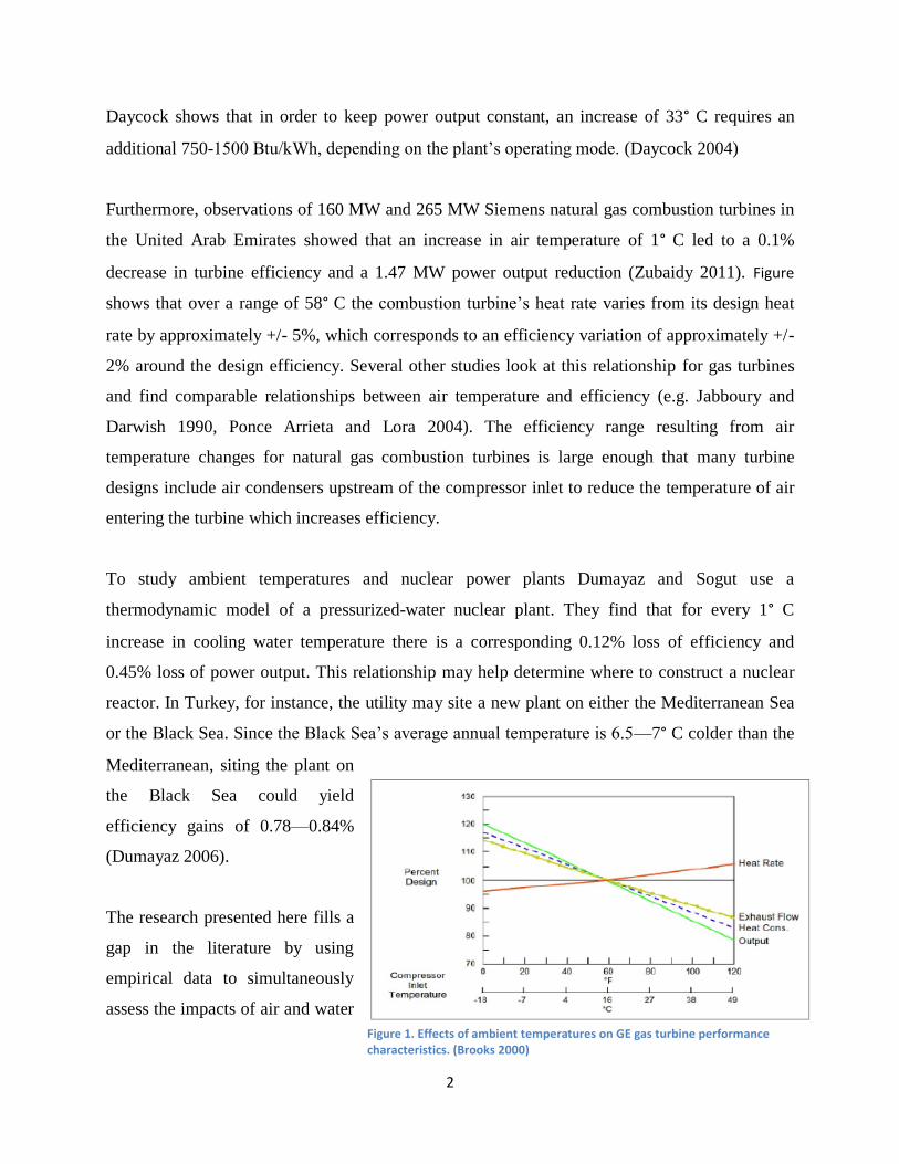
decrease in turbine efficiency and a 1.47 MW power output reduction (Zubaidy 2011). Figure
shows that over a range of 58° C the combustion turbine’s heat rate varies from its design heat
rate by approximately +/- 5%, which corresponds to an efficiency variation of approximately +/-
2% around the design efficiency. Several other studies look at this relationship for gas turbines
and find comparable relationships between air temperature and efficiency (e.g. Jabboury and
Darwish 1990, Ponce Arrieta and Lora 2004). The efficiency range resulting from air
temperature changes for natural gas combustion turbines is large enough that many turbine
designs include air condensers upstream of the compressor inlet to reduce the temperature of air
entering the turbine which increases efficiency.
To study ambient temperatures and nuclear power plants Dumayaz and Sogut use a
thermodynamic model of a pressurized-water nuclear plant. They find that for every 1° C
increase in cooling water temperature there is a corresponding 0.12% loss of efficiency and
0.45% loss of power output. This relationship may help determine where to construct a nuclear
reactor. In Turkey, for instance, the utility may site a new plant on either the Mediterranean Sea
or the Black Sea. Since the Black Sea’s average annual temperature is 6.5—7° C colder than the
Mediterranean, siting the plant on
the Black Sea could yield
efficiency gains of 0.78—0.84%
(Dumayaz 2006).
The research presented here fills a
gap in the literature by using
empirical data to simultaneously
assess the impacts of air and water
Figure 1. Effects of ambient temperatures on GE gas turbine performance characteristics. (Brooks 2000)

3
temperatures on a variety of generation technologies. There are four important differences
between the current research and previous studies. First, previous work examines air
temperatures or water temperatures individually rather than quantifying each environmental
variable using a common methodology. Second, this work examines the differential effects of air
and water temperatures across a variety of power generating technologies, comparing different
fuel types and cooling systems. We analyze 16 plants grouped into 4 categories based on fuel
type (natural gas and coal) and cooling system (once-through systems and recirculating systems)
to examine the relative temperature impacts on efficiency for each technology combination.
Third, this work focuses on fossil fuel-fired steam generators rather than combustion turbines or
nuclear generators. Finally, we use empirical data rather than physical or technological models
and compare results to the relationships found in the Integrated Environment Control Model
(IECM) to estimate the magnitude of each temperature-efficiency relationships.
The relationships found between temperatures and efficiency are smaller than relationships
previously reported by approximately one order of magnitude. For instance, we find that a 1° C
increase in air temperature is correlated with a change in plant efficiency of +0.02 to -0.03
percentage points and a 1° C increase in water temperature is correlated with a change in plant
efficiency of +0.02 to -0.06 percentage points. Previous work on water temperature and
efficiency has found a 0.12% decrease in efficiency for every 1° C temperature increase. Possible
explanations for the discrepancies between our work and previous results are offered in the
Discussion section. As shown below, the relationship we calculate between air temperature and
plant efficiency is similar to the relationship implied by the IECM model, but results from
studies of combustion turbines and air temperature have found relationships an order of
magnitude greater.
This paper is divided into 7 sections. Following the introduction, we describe the physical
relationships between ambient temperatures and plant efficiencies in section two. In the third
section data sources, data collection, and data selection processes are described. Section four
outlines the methodology used. Section five presents the results and section six is a discussion of
the results with practical implications. Section 7 is a conclusion.
4
II. Relationships between Ambient Temperatures and Efficiency
During the production of electricity, steam generators require oxygen during combustion and
water during the cooling process. Ambient air is drawn into the combustion chamber to provide
oxygen which is consumed in an exothermic combustion reaction whose heat is used to convert
water to pressurized steam. The steam drives a turbine and generates electricity. Once the steam
has expended its useful energy, it is cooled (typically using water, though not always), re-
condensing it into water to be boiled again.
The steam generator interacts with the environment at two stages. One is at the intake of ambient
air in the combustion process, and the second is when cooling water is drawn in for cooling.
Water may be obtained from various natural sources. Out of these two interactions, three
relationships are expected between ambient temperatures and power plant efficiency: two of
which relate air temperature and the efficiency of the combustion process, and the third relates
water temperature and plant efficiency.
Air Temperature and Efficiency
First, the temperatures of combustion for utility-scale generators typically reach 540° C or more
(Tsiklauri 2004), depending on the boiler technology. Oxygen in the air is used for combustion
and enters the plant at ambient temperatures usually below 50° C. Energy is expended raising the
temperature of the incoming air to the combustion temperature. Air entering the boiler at 40° C
requires relatively less energy to increase its temperature to 540° C than air entering the boiler at
-10° C. Therefore, warmer air is expected to provide an efficiency boost to a steam boiler.
Second, given a gas with constant mass, a temperature increase causes volumetric expansion and
a decrease in density. Consequently, the same volume of air will contain less oxygen at higher
temperature. Given a constant flow rate (volume of air per unit time) for a boiler’s air intake
system, an increase in temperature will decrease the rate of oxygen supplied to the boiler. Lower
levels of oxygen decrease the boiler’s efficiency. This magnitude of this effect is large enough
5
that many natural gas combustion turbines use condensers to cool incoming air. This effect of air
temperature on efficiency has the opposite direction of the first effect. Part of this analysis is
aimed at quantifying the overall effect of air temperature on efficiency, and whether the
magnitude of this effect is correlated with different fuel types or cooling systems.
Water Temperature and Efficiency
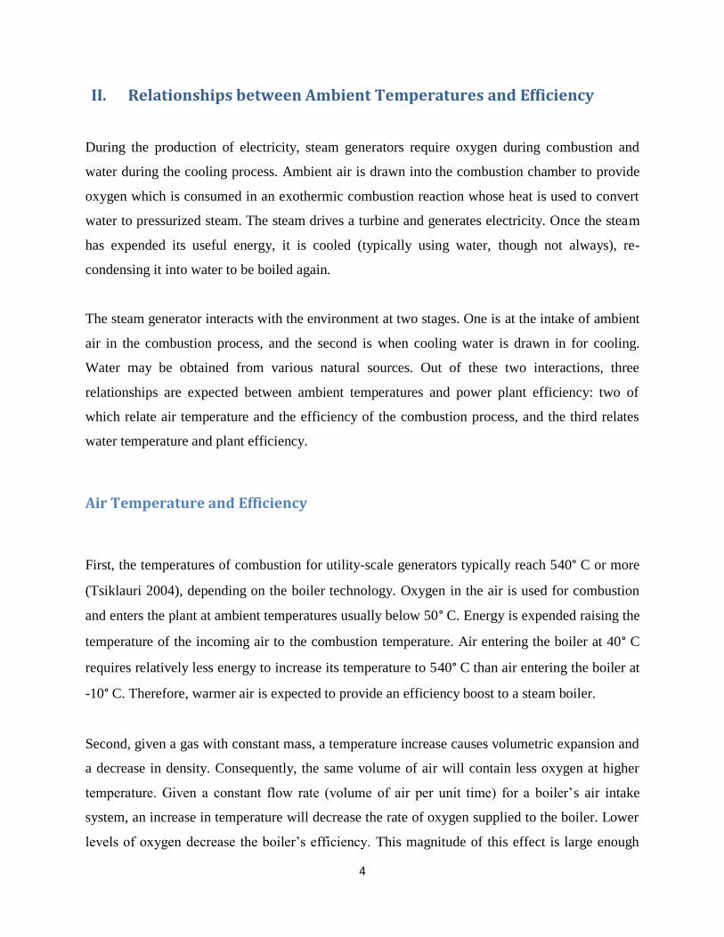
The third relationship relates water temperature and efficiency, and can be explained using the
Carnot equation for heat engine efficiency (see Figure and Equation 1). The equation indicates that
the Carnot efficiency of a heat engine is related to the temperature differential between the heat
source (TH) and the heat sink(TC). Given a heat source with constant temperature, as the
temperature of the heat sink increases, the Carnot efficiency will decrease.
III. Data Collection and Selection
Power Plant Data and Record Selection
EPA tracks hourly and daily electricity generation through its Clean Air Markets Division
(CAMD) for all power generators subject to emissions reporting requirements under EPA’s Acid
Rain Program, NOx Programs, or the Clean Air Interstate Rule (CAIR). Plant operators subject
to these air programs are required to report emissions, fuel consumption, and generating data,
which are included in the available dataset. (For the data source, see EPA 2013 in the References
section). The parameters relevant to this study are:
Figure 2. Diagram of a heat engine
Equation 1. Carnot efficiency for a heat engine.
6
1. Time of operation in each hour (h). A value of 1 indicates the plant was fully operational
for the hour of record, and a value of 0.5 indicates the plant only operated for 30 minutes
in the hour.
2. Heat input (q). This value is reported in million Btu (mmBtu) per hour.
3. Generation (g). The amount of electricity produced in the given hour is reported in
megawatt-hours (MWh).
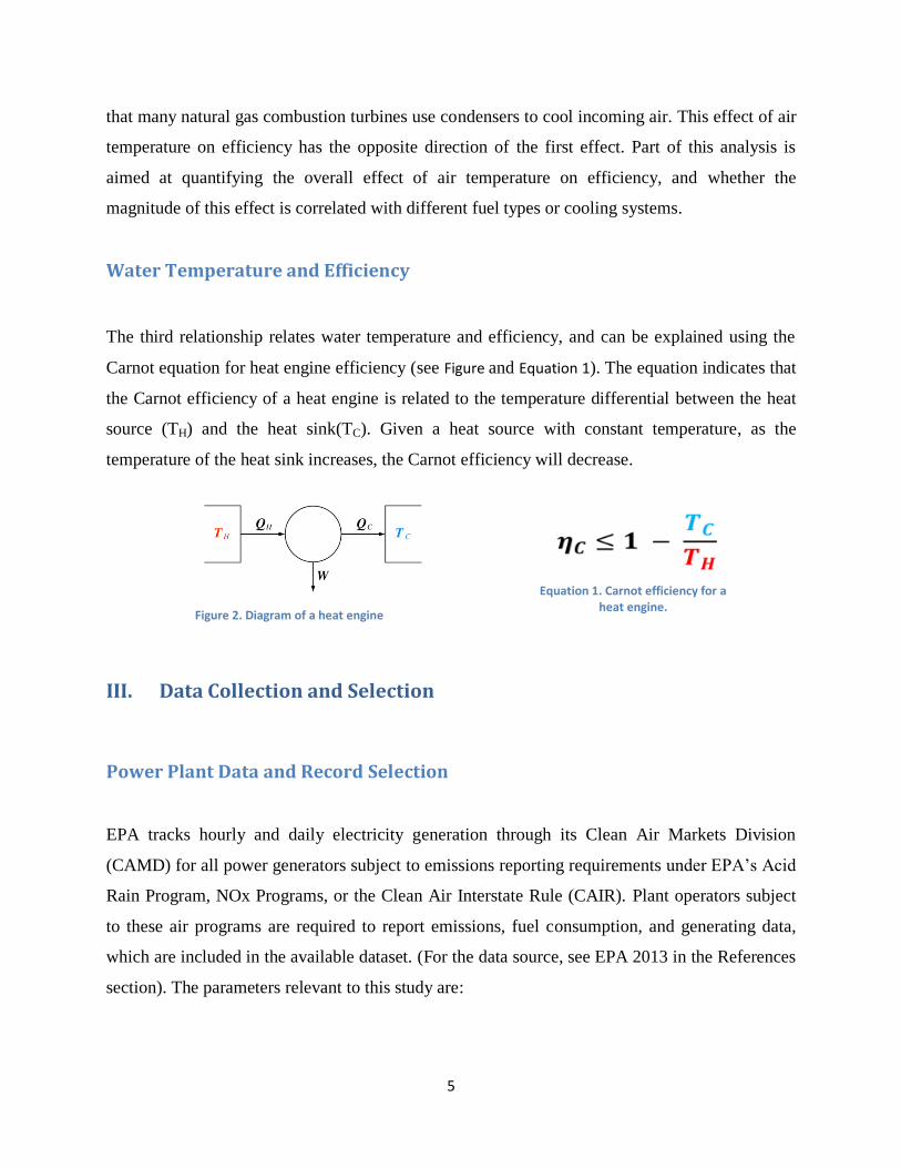
4. Plant efficiency (η) is calculated by converting the plant’s generation to mmBtu and
dividing by heat input, according to Equation 2:
Plant efficiency is the dependent variable for the regression models. Here we describe which
records are included in the regression analysis.
First, only hours during which the plant was operating for the full hour (h = 1) are included.
During hours of partial operation the efficiency could be affected by the plant’s efficiency while
ramping up or down. Furthermore, in most cases, hourly values were registered as either 0, 0.25,
0.5, 0.75, or 1 (corresponding to 0, 15, 30, 45, and 60 minutes). However, it seems unlikely that a
plant’s operations would be limited to 15 minute increments, suggesting lack of precision in
these particular records. In fact, there are numerous instances during hours of partial operation
where calculated efficiency is very close to or above 100% which is physically unlikely, but no
explanation for these efficiency levels is discernible from the data. For simplicity, hours of
partial operation are excluded from our analysis.
After excluding hours of partial operation there are still hours where efficiency is above 100%.
All of these records are excluded.
Efficiency varies significantly with power output. In order to control for power output, records
are selected based on the mode of each unit’s power output. In addition, this step removes many
instances in the dataset where efficiency is inexplicably high or low. Although this filtering
7
criterion removes a lot of available information, large numbers of records remain data for each
unit. Table 3 (see Appendix) Error! Reference source not found.shows the number of records
for each plant. For one generating unit, the mode of power output is 0 MW. For this unit, we
exclude hours with output of 0 MW and use the mode of the remaining records for analysis.
Finally, in the remaining data there are still anomalous efficiencies as high as 60%, 70% or 80%.
We found no explanation for these anomalies so we take a conservative approach regarding
which records to include. We exclude efficiency outliers defined as those beyond one
interquartile spread above or below the interquartile range, a common definition of outliers in
statistics.
Water Temperature Data
Two federal agencies maintain data on water temperature. The United States Geological Survey
(USGS) maintains monitors primarily in streams, rivers, and lakes around the country. These
monitors track a variety of water conditions, including flows, water levels, chemical properties,
and temperatures. The National Oceanic and Atmospheric Administration (NOAA) maintains
buoys and fixed monitoring stations deployed primarily along the US coastline and in the Great
Lakes. These buoys collect air and water temperature information as well as other climatic data.
(USGS 2012 and NOAA 2012)
Ideally, water temperature data would be collected precisely at the plant’s cooling water intake
valve. However, it was challenging to find monitors located on the same water body and within
several miles of power stations, and impossible to find temperature monitors located in the
immediate vicinity of power plant intake structures. For each plant we identify monitors
satisfying three conditions:
1. The monitor is located in the body of water from which the plant withdraws its cooling
water.
2. The monitor is close enough to the plant’s intake structure that relative changes in water
temperature at the monitor location are likely to reflect the relative change in water

8
temperature at the plant’s intake structure. (However, this condition may not be satisfied
for all plants, which is discussed in subsequent sections.)
3. Hourly data is available for the two year period coinciding with the hourly plant data
collected from EPA.
The distance between the power plant and the water monitor varies from 2.1 to 50.9 miles.
One shortcoming of this research is the lack of water temperature data with close proximity to
the power plants. As the distance between the plant’s intake structure and the water monitor
increases, the likelihood of thermal pollution between monitor and plant increases, reducing the
relevance of the data and the explanatory power of our results. We did not undertake any
analysis of the potential thermal sources affecting the quality of water temperature data.
Finally, water temperature data is obtained only for plants with a once-through cooling system,
and caution is taken to ensure that these plants do not store cooling water in cooling ponds whose
temperatures would not necessarily be correlated with data from monitoring stations.
Air Temperature and Dew Point Data
Air temperature and dew point data is
collected and distributed by the
National Climate Data Center
(NCDC), a division of NOAA. Using
NCDC’s Climate Data Online
application, we identify the weather
station closest to each power plant. As
with available water data, these data
do not reflect local temperatures at
power plants. Distances between
monitoring stations and power plants
Figure 1. Plant and unit breakdown by fuel type and cooling system.
9
range from 2.0 to 58.6 miles. Potentially confounding air temperature factors are briefly
described in the Discussion section.
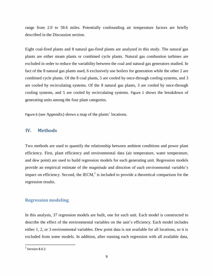
Eight coal-fired plants and 8 natural gas-fired plants are analyzed in this study. The natural gas
plants are either steam plants or combined cycle plants. Natural gas combustion turbines are
excluded in order to reduce the variability between the coal and natural gas generators studied. In
fact of the 8 natural gas plants used, 6 exclusively use boilers for generation while the other 2 are
combined cycle plants. Of the 8 coal plants, 5 are cooled by once-through cooling systems, and 3
are cooled by recirculating systems. Of the 8 natural gas plants, 3 are cooled by once-through
cooling systems, and 5 are cooled by recirculating systems. Figure 1 shows the breakdown of
generating units among the four plant categories.
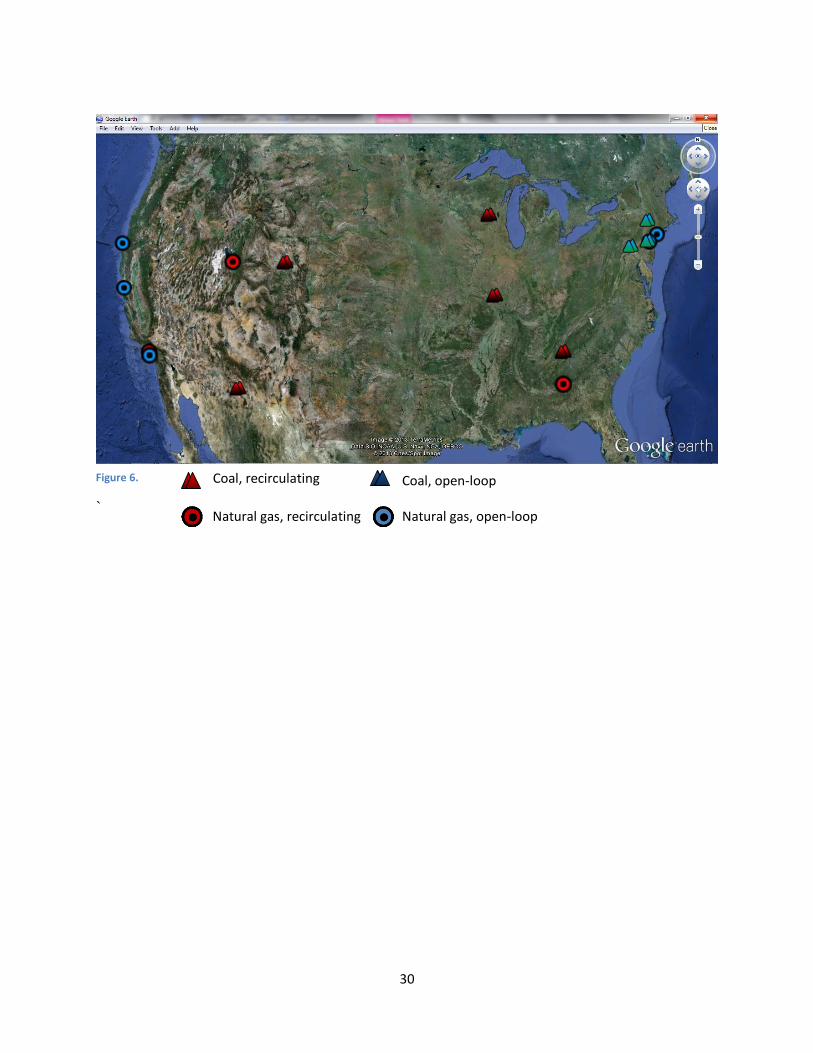
Figure 6 (see Appendix) shows a map of the plants’ locations.
IV. Methods
Two methods are used to quantify the relationship between ambient conditions and power plant
efficiency. First, plant efficiency and environmental data (air temperature, water temperature,
and dew point) are used to build regression models for each generating unit. Regression models
provide an empirical estimate of the magnitude and direction of each environmental variable’s
impact on efficiency. Second, the IECM,2 is included to provide a theoretical comparison for the
regression results.
Regression modeling
In this analysis, 37 regression models are built, one for each unit. Each model is constructed to
describe the effect of the environmental variables on the unit’s efficiency. Each model includes
either 1, 2, or 3 environmental variables. Dew point data is not available for all locations, so it is
excluded from some models. In addition, after running each regression with all available data,
2 Version 8.0.2

10
some of the environmental variables were determined to be not statistically significant in
explaining the efficiency of the respective units; these variables were removed from the final
model. Throughout this analysis, statistically significant figures imply regression coefficients
with p-values less than 0.05.
The reason for developing separate models for each unit3 is that environmental data comes from
a variety of sources which are likely to have varying degrees of accuracy. The assumption
implied by these models is that temperature data from air and water monitors reflect the power
plant’s local air and water temperatures, or at least that relative temperatures are consistent
between the monitors and power plants. There is reason to doubt this assumption, but we do not
investigate which monitors are “accurate” proxies of actual plant data. In a combined model,
inaccurate data would be mixed with accurate data; without knowing which monitoring data is
accurate, we keep each unit’s data separate and look at the temperature effects for each unit
individually.
To illustrate the variation in data, we describe two plant sites and their proximity to water
monitoring stations. The Humboldt Bay plant in Northern California is cooled by water from the
Pacific Ocean. The closest available water temperature data is collected from a NOAA buoy in
the Humboldt Bay 4 miles from the plant. However, the Port Jefferson plant is located on Staten
Island and is cooled by water from the Arthur Kill, which is a narrow strait separating Staten
Island from New Jersey. Water temperature data for the Port Jefferson plant is collected from a
buoy in the New York Harbor, also about 4 miles away. However, the two cooling water sources
for these two plants are very different in size, shape, and in commercial activity in the water
body. It might be expected that water temperatures between Port Jefferson and the water
monitor are affected by many local sources of thermal pollution, such as boat traffic or other
industrial discharges, whereas, there are fewer sources of thermal discharge in Humboldt Bay,
California. Rather than attempting to mitigate confounding sources of thermal pollution, or
simply excluding the New York plant, we analyze each plant individually, and exclude variables
based on their statistical significance in each model.
3 Nested and fixed effects regression models were also considered for this analysis.
11
Several regressions were run before arriving at the final model. In the first set of regressions, a
model is built for each of the 37 units. For plants with once-through cooling systems, efficiency
is regressed against air temperature, water temperature and dew point. Whereas regression
models for plants with recirculating systems only incorporate air temperature and dew point.
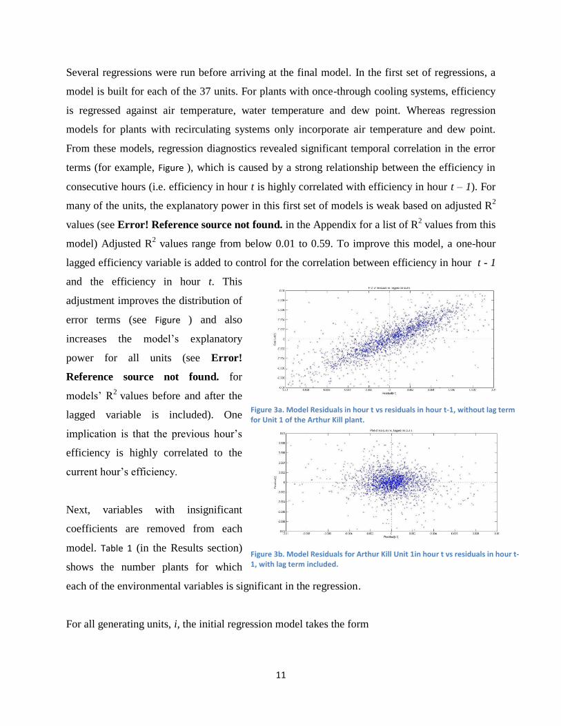
From these models, regression diagnostics revealed significant temporal correlation in the error
terms (for example, Figure ), which is caused by a strong relationship between the efficiency in
consecutive hours (i.e. efficiency in hour t is highly correlated with efficiency in hour t – 1). For
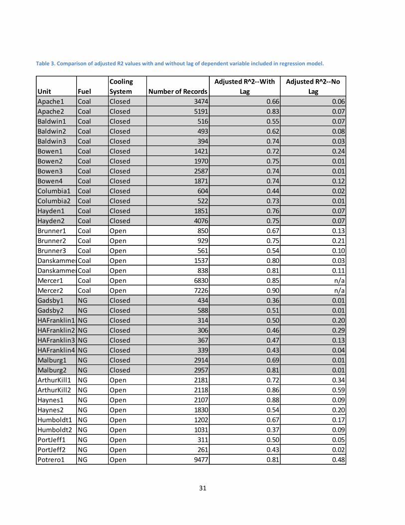
many of the units, the explanatory power in this first set of models is weak based on adjusted R2
values (see Error! Reference source not found. in the Appendix for a list of R2 values from this
model) Adjusted R2 values range from below 0.01 to 0.59. To improve this model, a one-hour
lagged efficiency variable is added to control for the correlation between efficiency in hour t - 1
and the efficiency in hour t. This
adjustment improves the distribution of
error terms (see Figure ) and also
increases the model’s explanatory
power for all units (see Error!
Reference source not found. for
models’ R2
values before and after the
lagged variable is included). One
implication is that the previous hour’s
efficiency is highly correlated to the
current hour’s efficiency.
Next, variables with insignificant
coefficients are removed from each
model. Table 1 (in the Results section)
shows the number plants for which
each of the environmental variables is significant in the regression.
For all generating units, i, the initial regression model takes the form
Figure 3a. Model Residuals in hour t vs residuals in hour t-1, without lag term for Unit 1 of the Arthur Kill plant.
Figure 3b. Model Residuals for Arthur Kill Unit 1in hour t vs residuals in hour t-1, with lag term included.

12
where,
However, for each unit, terms are removed from the final regression model depending on the
significance of the independent variable.
Modeling Using the IECM
The IECM allows users to design a power plant using a wide variety of technical, operating,
emissions technology, ambient, and financial specifications. As mentioned above, the relevant
parameters for this study are:
1. Fuel type
2. Cooling system
3. Air temperature
4. Water temperature
Eight coal combustion and 2 natural gas combined cycle plants are modeled. Four of the coal
plants are modeled with a once-through cooling system and 4 with a recirculating system. For

13
each type of cooling system, we set the coal plant’s capacity to 100, 200, 500, and 1000 MW to
analyze the effect of plant size on the temperature-efficiency relationship. The IECM model does
not allow the user to determine the size of the combustion turbine, so it is not possible to control
the NG plant size in the same way,4 so we only model two NG plants, one for each cooling
system.
IECM allows the user to change the ambient air temperature, but not the ambient water
temperature. For each plant, the ambient air temperature is set to 15°F, 36.25°F, 57.5°F, 78.25°F
and 100° and the associated efficiencies are recorded to capture the IECM model’s predicted
effect of air temperature on plant efficiency.
In setting the plant size, the IECM natural gas plant can include one of two turbine models (GE
7FB and GE 7FA) and 1, 2, 3, 4, or 5 turbines. We use one GE 7FB, whose gross power output
of 454.3 MW and net output is 264.4 MW. Changing the number of turbines does not affect the
net efficiency of the plant. For the NG portion of IECM modeling we do not vary plant size.
V. Results
First, we summarize the effects predicted by the multivariate regression model developed from
actual plant data; second, we discuss results from the IECM model.
Regression Modeling
For each generating unit, the regression coefficient estimates the correlation between a one-unit
increase in the environmental variable (i.e. degree Celsius or dew point) and change in the unit’s
efficiency, in terms of percentage points gained or lost. For example, if a unit whose water
temperature coefficient, 3 is -0.01, that unit experiences an efficiency loss of 0.01 percentage
points for every 1° C increase in water temperature, all else being equal. More specifically, if a
4 The parameters controlling the capacity of the NG plant are the gas turbine model (GE 7FA or GE 7FB) and the
number of turbines used in the plant. The two turbine models are roughly the same size, and varying the number of units has no impact on the plant’s efficiency.

14
coal plant with a once-through cooling system is generating electricity with 35.00% efficiency
and its cooling water temperature increases from 20° C to 21° C, its efficiency will drop to
34.99%.
Plant type and statistical significance of environmental variables
Table 1 and Table 4 (see Appendix) show which environmental variables are significant for each
power plant category. Table 1 shows the number of plants where efficiency is statistically
correlated (p < 0.05) to each of the independent environmental variables. Overall, air temperature
is found to be significantly correlated with efficiency for 17 out of 37 units; water temperature is
significant for 12 out of 16 units, and dew point is significant for 14 out of 29 units.
Table 4 (see Appendix) summarizes which combinations of environmental variables are
statistically significant for the units within each plant category. For example, there are 9 units
powered by natural gas with once-through cooling systems. Among these 9 units, efficiency is
correlated with air and water temperature at 2 units; however for 2 other units, efficiency is only
correlated with air temperature (it is not correlated with any other environmental variables); and
for 5 units, efficiency is only correlated with water temperature. Dew point is not significantly
correlated with efficiency for any of the once-through natural gas plants.
Fuel
Type
Cooling
System
Number of
Units Where
Data is
Available
Air Temp
Significant in
Regression on
Efficiency
Number of
Units Where
Data is
Available
Water Temp
Significant in
Regression on
Efficiency
Number of
Units Where
Data is
Available
Dew Point
Significant in
Regression on
Efficiency
Coal Recirculating 13 5 N/A N/A 13 7
Coal Once through 7 4 7 6 4 3
NG Recirculating 8 5 N/A N/A 8 4
NG Once through 9 4 9 6 4 0
Totals 37 18 16 12 29 14
Air Temp Water Temp Dew Point
Table 1. Number of plants where efficiency is significantly affected by ambient variables.
15
Size and direction of temperature effects
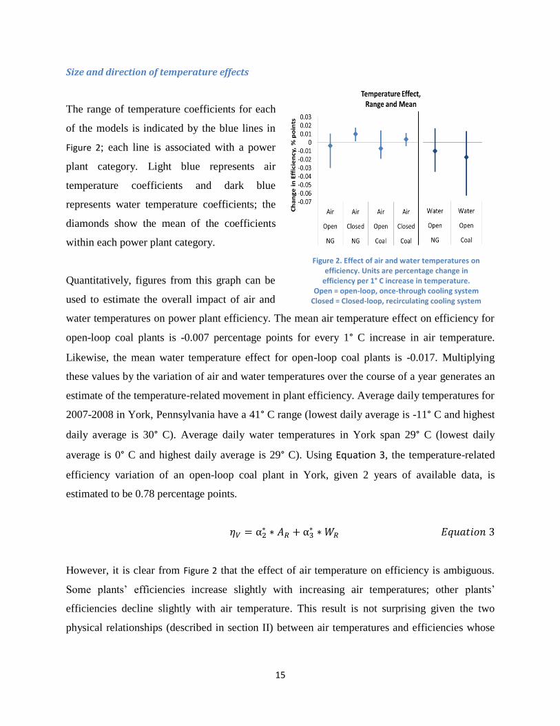
The range of temperature coefficients for each
of the models is indicated by the blue lines in
Figure 2; each line is associated with a power
plant category. Light blue represents air
temperature coefficients and dark blue
represents water temperature coefficients; the
diamonds show the mean of the coefficients
within each power plant category.
Quantitatively, figures from this graph can be
used to estimate the overall impact of air and
water temperatures on power plant efficiency. The mean air temperature effect on efficiency for
open-loop coal plants is -0.007 percentage points for every 1° C increase in air temperature.
Likewise, the mean water temperature effect for open-loop coal plants is -0.017. Multiplying
these values by the variation of air and water temperatures over the course of a year generates an
estimate of the temperature-related movement in plant efficiency. Average daily temperatures for
2007-2008 in York, Pennsylvania have a 41° C range (lowest daily average is -11° C and highest
daily average is 30° C). Average daily water temperatures in York span 29° C (lowest daily
average is 0° C and highest daily average is 29° C). Using Equation 3, the temperature-related
efficiency variation of an open-loop coal plant in York, given 2 years of available data, is
estimated to be 0.78 percentage points.
However, it is clear from Figure 2 that the effect of air temperature on efficiency is ambiguous.
Some plants’ efficiencies increase slightly with increasing air temperatures; other plants’
efficiencies decline slightly with air temperature. This result is not surprising given the two
physical relationships (described in section II) between air temperatures and efficiencies whose
Figure 2. Effect of air and water temperatures on efficiency. Units are percentage change in
efficiency per 1° C increase in temperature. Open = open-loop, once-through cooling system
Closed = Closed-loop, recirculating cooling system
16
effects oppose each other. Moreover, nearly half of the plants analyzed did not exhibit any
correlation between air temperature and plant efficiency.
Although the overall effect of air temperature on plant efficiency is uncertain and fairly small,
there appears to be a correlation between the cooling system and the direction of efficiency. The
efficiency of natural gas and coal plants with closed-loop cooling systems both tend to exhibit a
positive correlation with air temperature, but the efficiency of open-loop systems tends to exhibit
a negative correlation. This result was not expected based on the analysis of temperature and
efficiency relationships. (However, one possible explanation is presented in the Discussion.)
Furthermore, the air temperature-efficiency relationship for open loop plants is mirrored in the
water temperature-efficiency relationship, suggesting that these two variables are covariates
which could weaken the regression modeling results. Two arguments refute this. First, there are
14 once-through generating units whose efficiency is statistically impacted by air and water
temperature. However, only 4 of those units are affected by both air and water temperature,
while the other 10 units are only affected by one variable or the other. Efficiencies at 7 plants are
statistically correlated only with water temperature; at 3 plants efficiency is only correlated with
air temperature; and at 1 plant efficiency is statistically correlated with both air temperature and
dew point.
Second, the same regression was run with an interaction term between air and water
temperatures. For nearly all the units’ regressions, the coefficient on the interaction term was
insignificant, or the models’ power to explain the dependent variable (measured by the adjusted
R2) decreased dramatically with the interaction term, both of which indicate that the relationship
between air and water temperature is not weakening the model. One additional concern which
has not been tested is the possibility that even though air and water temperatures are not strong
covariates at hour t, there may be a more significant relationship between air and water
temperatures when a time lag is introduced.
17
Regarding water temperature and plant efficiency, the data show a clearer trend that increasing
water temperatures are correlated with decreasing plant efficiencies for both coal and natural gas
plants. This relationship is predicted by Carnot’s equation.
Though dew point is included in the regression models, we do not describe in detail its impact on
plant efficiency. For the majority of units, dew point is not a significant indicator of efficiency.
Furthermore, of the 13 units where dew point is statistically significant, the regression coefficient
on dew point for 8 of these units is an order of magnitude smaller than that of air or water
temperature. Thus, if included in Figure 2, the range of dew points would be nearly invisible and
not discernible from zero.
IECM Model
Coal Plants
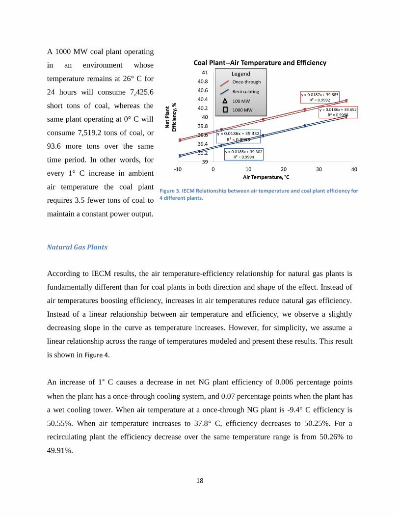
Figure 3 shows the relationship between air temperature and plant net efficiency for four plants
modeled using IECM. The 1000 MW plant is slightly more efficient than the 100 MW plant: at
any given temperature, the 1000 MW plant’s net efficiency is 0.03 percentage points higher than
the 100 MW plant. Figure 3 shows that once-through plants have a higher net efficiency than
recirculating plants. However, the gross efficiency of each plant is constant for both cooling
types; the difference is caused by parasitic power consumption required to run the cooling tower.
According to IECM modeling results, there is a direct linear relationship between ambient air
temperatures and efficiency for coal plants: as the temperature increases by 1° C, the plant’s net
efficiency increases 0.02 percentage points, when other variables are held constant. This
relationship holds across cooling system types and plant sizes. The IECM model allows for the
user to adjust temperatures within the range -9.4° C (15° F) to 37.8° C (100° F). When the
ambient temperature is 37.8° C, the coal plant’s net efficiency (for all plant sizes and cooling
types) is 0.8 percentage points higher than when temperature is -9.4° C.
18
A 1000 MW coal plant operating
in an environment whose
temperature remains at 26° C for
24 hours will consume 7,425.6
short tons of coal, whereas the
same plant operating at 0° C will
consume 7,519.2 tons of coal, or
93.6 more tons over the same
time period. In other words, for
every 1° C increase in ambient
air temperature the coal plant
requires 3.5 fewer tons of coal to
maintain a constant power output.
Natural Gas Plants
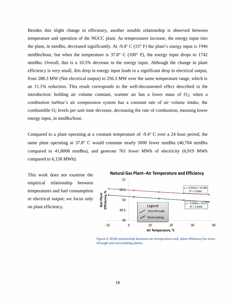
According to IECM results, the air temperature-efficiency relationship for natural gas plants is
fundamentally different than for coal plants in both direction and shape of the effect. Instead of
air temperatures boosting efficiency, increases in air temperatures reduce natural gas efficiency.
Instead of a linear relationship between air temperature and efficiency, we observe a slightly
decreasing slope in the curve as temperature increases. However, for simplicity, we assume a
linear relationship across the range of temperatures modeled and present these results. This result
is shown in Figure 4.
An increase of 1° C causes a decrease in net NG plant efficiency of 0.006 percentage points
when the plant has a once-through cooling system, and 0.07 percentage points when the plant has
a wet cooling tower. When air temperature at a once-through NG plant is -9.4° C efficiency is
50.55%. When air temperature increases to 37.8° C, efficiency decreases to 50.25%. For a
recirculating plant the efficiency decrease over the same temperature range is from 50.26% to
49.91%.
Figure 3. IECM Relationship between air temperature and coal plant efficiency for 4 different plants.
19
Besides this slight change in efficiency, another notable relationship is observed between
temperature and operation of the NGCC plant. As temperatures increase, the energy input into
the plant, in mmBtu, decreased significantly. At -9.4° C (15° F) the plant’s energy input is 1946
mmBtu/hour, but when the temperature is 37.8° C (100° F), the energy input drops to 1742
mmBtu. Overall, this is a 10.5% decrease in the energy input. Although the change in plant
efficiency is very small, this drop in energy input leads to a significant drop in electrical output,
from 288.3 MW (Net electrical output) to 256.3 MW over the same temperature range, which is
an 11.1% reduction. This result corresponds to the well-documented effect described in the
introduction: holding air volume constant, warmer air has a lower mass of O2; when a
combustion turbine’s air compression system has a constant rate of air volume intake, the
combustible O2 levels per unit time decrease, decreasing the rate of combustion, meaning lower
energy input, in mmBtu/hour.
Compared to a plant operating at a constant temperature of -9.4° C over a 24 hour period, the
same plant operating at 37.8° C would consume nearly 5000 fewer mmBtu (46,704 mmBtu
compared to 41,8008 mmBtu), and generate 761 fewer MWh of electricity (6,919 MWh
compared to 6,158 MWh).
This work does not examine the
empirical relationship between
temperatures and fuel consumption
or electrical output; we focus only
on plant efficiency.
Figure 4. IECM relationship between air temperature and plant efficiency for once-through and recirculating plants.
20
VI. Discussiom
Comparing Regression modeling and IECM results
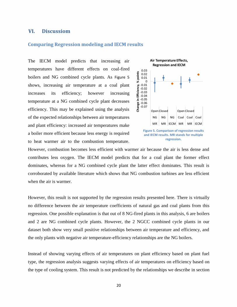
The IECM model predicts that increasing air
temperatures have different effects on coal-fired
boilers and NG combined cycle plants. As Figure 5
shows, increasing air temperature at a coal plant
increases its efficiency; however increasing
temperature at a NG combined cycle plant decreases
efficiency. This may be explained using the analysis
of the expected relationships between air temperatures
and plant efficiency: increased air temperatures make
a boiler more efficient because less energy is required
to heat warmer air to the combustion temperature.
However, combustion becomes less efficient with warmer air because the air is less dense and
contributes less oxygen. The IECM model predicts that for a coal plant the former effect
dominates, whereas for a NG combined cycle plant the latter effect dominates. This result is
corroborated by available literature which shows that NG combustion turbines are less efficient
when the air is warmer.
However, this result is not supported by the regression results presented here. There is virtually
no difference between the air temperature coefficients of natural gas and coal plants from this
regression. One possible explanation is that out of 8 NG-fired plants in this analysis, 6 are boilers
and 2 are NG combined cycle plants. However, the 2 NGCC combined cycle plants in our
dataset both show very small positive relationships between air temperature and efficiency, and
the only plants with negative air temperature-efficiency relationships are the NG boilers.
Instead of showing varying effects of air temperatures on plant efficiency based on plant fuel
type, the regression analysis suggests varying effects of air temperatures on efficiency based on
the type of cooling system. This result is not predicted by the relationships we describe in section
Figure 5. Comparison of regression results and IECM results. MR stands for multiple
regression.

21
II, in fact, it is difficult to imagine how different cooling systems could interact with air
temperatures to have opposing effects on plant efficiency.
One possible explanation has to do with how the different cooling systems deal with thermal
waste. Once-through cooling systems dispose of excess heat fairly rapidly. Cooling water enters
the plant, removes heat from the steam, and is discharged back into the water body, carrying with
it waste heat. However, for recirculating systems, cooling water enters the plant, removes heat
from the steam, but then recirculates through the cooling system, getting hotter and hotter.
Cooling towers are usually incorporated into recirculating cooling systems to allow the built-up
waste heat to escape to the environment in the form of water vapor. Overall, plants with
recirculating systems retain much more of the waste heat than those with once-through cooling
systems, but perhaps more importantly, heat from recirculating systems is released much closer
to the plant itself. Rather than discharging heat into the river and carried downstream, the heat is
released into the plant’s immediate vicinity in the form of water vapor. Perhaps there is a
temperature feedback loop at plants with recirculating systems, where released heat increases the
local temperature. The extra heat released from cooling towers is unlikely to appear in our data
set since monitors are not onsite. However, discharging excess heat through the cooling towers
may be more efficient when ambient temperatures are lower, whereas when ambient
temperatures are higher, more of the discharged heat remains closer to the plant. Assuming
warmer air increases efficiency, this feedback loop between ambient temperatures and
temperatures in the plant’s immediate vicinity would lead to even greater efficiency at plants
with recirculating cooling systems than those with once-through cooling systems.
Explanation of insignificant environmental variables
There are a couple physical rationales to explain why in some instances the dependent variables
may not be significant predictors of the independent variable. First, the water and air temperature
monitors are not close to the power plants themselves. Though we would expect the relative
temperature changes at the monitoring stations to reflect temperature changes at the plants, there
could be thermal inputs to the water or air between the monitors and the plants that is not
measured by the temperature monitors. These heat sources which could be other power plants or
22
factories, heat island effects from urban centers or other concrete surfaces, local weather
conditions, or even heat created by the power plants themselves would introduce variation in
temperature not captured by this data. Potentially confounding heat sources are not examined in
this analysis.
Second, there may be unexplored, unidentified factors related to the plants’ operating
characteristics which reduce the plants’ sensitivity to air or water temperatures.
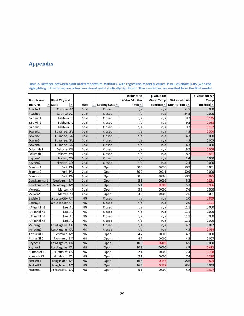
For reference, Table 2 (see appendix) shows the plants’ locations, distances between monitors and
plants, and the raw p-values for each regression coefficient (before removing the insignificant
variables).
We do observe that statistical significance of the dependent variables is generally consistent
across generating units within a particular plant. For example, for the Mercer plant’s regression,
coefficients of air temperature are statistically significant for both units 1 and 2 (p < 0.01);
whereas at the Danskammer plant, the coefficients for both units 1 and 2 are not statistically
significant (p = 0.88 and 0.94, respectively). This result suggests either consistently poor data
quality for the Danskammer plant and consistently better data quality for the Mercer plant or that
an unmeasured variable is far more important than temperature in determining the efficiency of
the Danskammer plant, but which is not impacting the Mercer plant.
However, there are four instances where the statistical significance for the same parameter at the
same plant is dramatically different between the plant’s generating units. The water temperature
for unit 1 of the Haynes plant is not statistically significant (p = 0.40) but for unit 2 of the same
plant water temperature is significant (p < 0.01). Also at the Haynes plant, air temperature is
statistically significant for unit 1 (p < 0.01) but not for unit 2 (p= 0.48). Similar discrepancies can
be seen for the air temperature’s significance levels between Port Jefferson’s units 1 and 2 as
well as for the water temperature significance between Danskammer’s units 1 and 2. These
results are odd. One confounding feature of the Haynes and Port Jefferson plants is that can be
co-fired using oil. Typically, oil is used to ramp up a plant to its desired capacity, and it is
possible that oil may be used as fuel during additional periods. However, the EPA data does not
23
indicate which fuel is used in a given hour. If available, this data would have offered important
insight since different fuel types in dual-fueled boilers could have a much larger impact on the
unit’s efficiency than would any changes in air or water temperatures.
Comparison with previous studies
The paper by Vliet et al. published in Nature describes a more substantial impact of a changing
climate on power plant operations than is suggested by results presented here. This impact is the
result of increased variation in both cooling water availability and temperature, which causes
plants to shut down or curtail generation to avoid surpassing regulatory limits. Their work also
points out that as cooling capacity decreases with increasing water temperature, power output
will necessarily decrease as well. Reduced power output is likely to affect power plant
efficiency. Our work attempts to isolate the effect of ambient temperatures on efficiency by
eliminating variation in power output. We do however observe strong correlations between
power output and efficiency showing that a decrease in power output is associated with a
decrease in plant efficiency. Although efficiency impacts are merely implied by the scenarios
described by Vliet, et al., they are not explicitly quantified. This goal of this work has been to
quantify the relationship between temperatures and power plant efficiency.
There is some discrepancy between our results and the temperature impacts on efficiency found
in the literature. Previous studies find that a 1° C air temperature increase leads an efficiency
decrease of over 0.1 percentage points for natural gas combustion turbines, whereas the
regression analysis presented here suggests a range of effects from -0.03 (decrease) to +0.02
(increase) percentage points per degree Celsius. This difference is most likely a result of
different generation technologies studied. Natural gas turbines are particularly sensitive to air
temperature compared to thermal steam generation plants. Furthermore, our results are consistent
with estimates of the air temperature-efficiency effect implied by the IECM model.
Looking at water temperature and the efficiency of a pressurized-water nuclear reactor, Dumayaz
found that a 1° C water temperature increase is correlated with an efficiency decrease of 0.12
24
percentage points. Our regression analysis suggests a range of efficiency changes from -0.06
(decrease) to +0.02 (increase). The nuclear plant may be more sensitive to cooling water
temperature changes because the temperature inside the reactor (TH in Carnot’s equation) is 325°
C (World Nuclear Association 2013) which is much lower than the 540° C temperatures inside
coal and natural gas boilers (Tsiklari 2004). Analysis of the Carnot equation shows that a 1° C
change in cooling water temperature (TC) will have a larger effect on Carnot efficiency when TH
is lower.
Alternatively, it is possible that the temperature signal is reduced when regressed against
efficiency as a result of thermal noise occurring between the air and water temperature monitors
and the actual power plant. This is discussed above in the “Explanation of insignificant
environmental variables” subsection.
Relevance of results
Variation explained by temperature changes compared to overall variation of power plants
Each power plant in this study operates at a range of efficiencies throughout the year. The
regression results indicate that air and water temperatures are not the only factors that vary with
efficiency. In fact, it appears that a large portion of the variation in plant efficiency cannot be
explained by the relationship between ambient temperatures and efficiency. Holding power
output constant, the efficiency variation over the course of a year for a generating unit is as low
as 1.5 percentage points and as high as 9.0 percentage points. The average efficiency variation
for the units studied is 3.9 percentage points.
In the Results section, the efficiency variation due to ambient temperature changes is estimated
to be 0.78 percentage points for the open-loop coal plant in York, PA. The total observed
efficiency variations for the three units of this York plant are 4.0, 6.0, and 6.0 percentage points.
Therefore, the change in efficiency due to temperature changes throughout the course of a year
explains only a fraction of the overall changes in efficiency.
25
Notably, assuming that plant efficiency varies by 0.12 percentage points per 1° C change in
water temperature (Dumayaz), a 25° C water temperature range would lead to a 3% efficiency
range, which is more consistent with the actual efficiency range experienced by the plants in this
study.
Implications of 5° C increase for plant efficiency, fuel consumption, fuel cost, and emissions
Although the effect of temperature changes on power plant efficiency is small in percentage
terms, this effect is noticeable in terms of fuel costs. Here we look at the potential impact of a 5°
C increase in air and water temperatures on fuel costs for an 800 MW coal plant. For simplicity,
we assume the plant has an average annual efficiency of 40%, a capacity factor of 70%, and that
the 5° C increase in air and water temperatures applies to all hours of the year.5
The hypothetical plant consumes 1,743,532 short tons of coal each year. Using the average air
and water temperature parameters (∝2 = -0.007 for air and ∝3 = -0.017 for water), the decrease in
efficiency associated with a 5° C temperature increase will be 0.12 percentage points. To
maintain its power output of 800 MW, the plant requires 5,246 additional short tons of coal.
Using the 2011 average coal price of $32.56 per short ton (EIA 2012), this decrease in efficiency
represents an increased cost of $170,821 per year.
Finally, using EIA emission factors (Hong and Slatick 1994), 5,246 tons of bituminous coal
represents 12,925 tons of CO2 emissions.
VII. Conclusion
This study analyzes empirical data from thermoelectric power plants and temperature monitoring
stations. Using multivariate regression, relationships between power plant efficiency and air and
water temperatures are estimated for a variety of power plant types. For natural gas and coal
plants with an open-loop cooling system a 1° C increase in air temperatures is correlated with a
mean change in plant efficiency of -0.004 and -0.007 percentage points, respectively. For natural
5 This assumption is particularly unrealistic but is used for illustration.

26
gas and coal plants with a recirculating cooling system, a 1° C increase in air temperature is
correlated with a mean change in plant efficiency of 0.009 and 0.004 percentage points,
respectively. A 1° C increase in water temperatures is correlated with a mean efficiency change
of -0.01 and -0.02 percentage points for natural gas and coal plants.
These relationships are smaller in magnitude than reported by previous studies, which is likely a
result of different methodologies, different technologies analyzed, and possibly due to data
sources used in this study. Furthermore, regression results obtained in this study suggest that the
variation in power plant efficiency is only partially explained by the variation in air and water
temperatures.
Future iterations of this work may benefit from analyzing in greater detail the operating
parameters at one or two power plants, confirming the accuracy of ambient temperature and
plant efficiency data, or using another analytic method to compare this data. The conclusions we
present contrasts with recent reports published in leading journals stating the dramatic impact of
climate change on the power sector.
In the context of climate change, the effects quantified here pose relatively small risks to the
power sector, especially given the gradual nature of global temperature changes. The temperature
variation experienced by power plants over the course of a year, or even the course of a day is
more dramatic than the expected change in temperatures over the next hundred years. However,
any loss of efficiency will be experienced by all thermoelectric generators which account for the
vast majority of power generation across the US and around the world. By calculating the
magnitude of the relationship between ambient temperatures and plant efficiency, the current
work helps determine the relative importance of the risk of rising temperatures for the power
sector among the myriad risks created by a changing global climate.
27
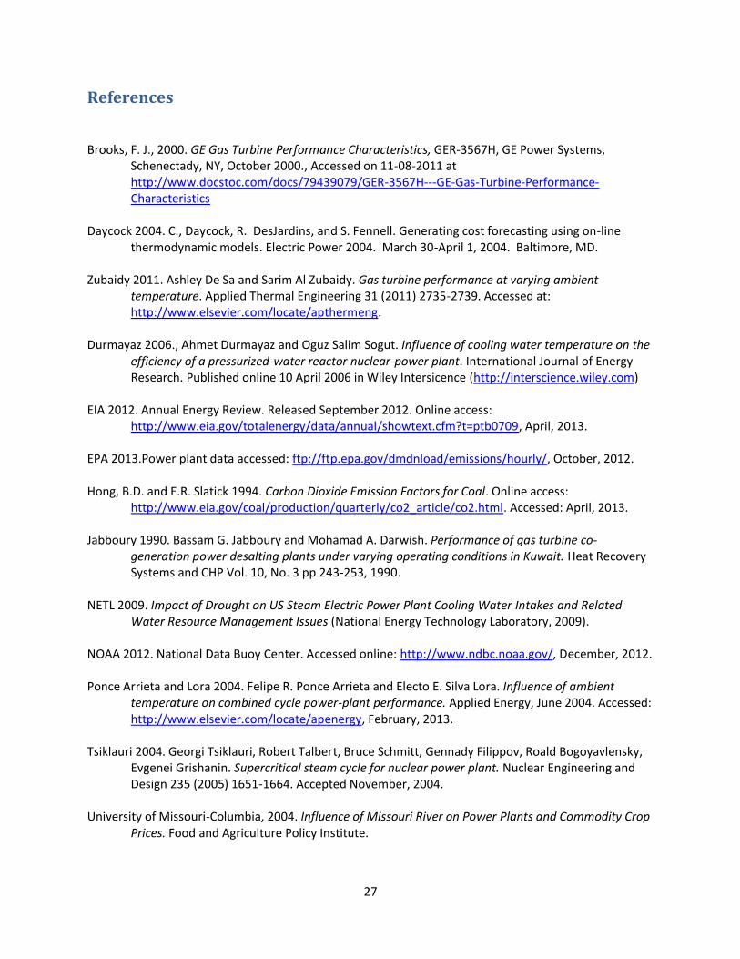
References
Brooks, F. J., 2000. GE Gas Turbine Performance Characteristics, GER-3567H, GE Power Systems, Schenectady, NY, October 2000., Accessed on 11-08-2011 at http://www.docstoc.com/docs/79439079/GER-3567H---GE-Gas-Turbine-Performance-Characteristics
Daycock 2004. C., Daycock, R. DesJardins, and S. Fennell. Generating cost forecasting using on-line
thermodynamic models. Electric Power 2004. March 30-April 1, 2004. Baltimore, MD. Zubaidy 2011. Ashley De Sa and Sarim Al Zubaidy. Gas turbine performance at varying ambient
temperature. Applied Thermal Engineering 31 (2011) 2735-2739. Accessed at: http://www.elsevier.com/locate/apthermeng.
Durmayaz 2006., Ahmet Durmayaz and Oguz Salim Sogut. Influence of cooling water temperature on the
efficiency of a pressurized-water reactor nuclear-power plant. International Journal of Energy Research. Published online 10 April 2006 in Wiley Intersicence (http://interscience.wiley.com)
EIA 2012. Annual Energy Review. Released September 2012. Online access:
http://www.eia.gov/totalenergy/data/annual/showtext.cfm?t=ptb0709, April, 2013. EPA 2013.Power plant data accessed: ftp://ftp.epa.gov/dmdnload/emissions/hourly/, October, 2012. Hong, B.D. and E.R. Slatick 1994. Carbon Dioxide Emission Factors for Coal. Online access:
http://www.eia.gov/coal/production/quarterly/co2_article/co2.html. Accessed: April, 2013. Jabboury 1990. Bassam G. Jabboury and Mohamad A. Darwish. Performance of gas turbine co-
generation power desalting plants under varying operating conditions in Kuwait. Heat Recovery Systems and CHP Vol. 10, No. 3 pp 243-253, 1990.
NETL 2009. Impact of Drought on US Steam Electric Power Plant Cooling Water Intakes and Related
Water Resource Management Issues (National Energy Technology Laboratory, 2009). NOAA 2012. National Data Buoy Center. Accessed online: http://www.ndbc.noaa.gov/, December, 2012. Ponce Arrieta and Lora 2004. Felipe R. Ponce Arrieta and Electo E. Silva Lora. Influence of ambient
temperature on combined cycle power-plant performance. Applied Energy, June 2004. Accessed: http://www.elsevier.com/locate/apenergy, February, 2013.
Tsiklauri 2004. Georgi Tsiklauri, Robert Talbert, Bruce Schmitt, Gennady Filippov, Roald Bogoyavlensky,
Evgenei Grishanin. Supercritical steam cycle for nuclear power plant. Nuclear Engineering and Design 235 (2005) 1651-1664. Accepted November, 2004.
University of Missouri-Columbia, 2004. Influence of Missouri River on Power Plants and Commodity Crop
Prices. Food and Agriculture Policy Institute.

28
USGS 2012. WaterWatch. Accessed online: http://waterwatch.usgs.gov/?id=ww_current, December 2012.
World Nuclear Association 2013. Nuclear Power Reactors. Updated December, 2012. Accessed online:
http://www.world-nuclear.org/info/Nuclear-Fuel-Cycle/Power-Reactors/Nuclear-Power-Reactors/#.UXce57WG2So, March 2013.
29
Appendix
Plant Name
and Unit
Plant City and
State Fuel Cooling System
Distance to
Water Monitor
(miles)
p-value for
Water Temp
coefficient
Distance to Air
Monitor (miles)
p-Value for Air
Temp
coefficient
Apache1 Cochise, AZ Coal Closed n/a n/a 54.5 0.000
Apache2 Cochise, AZ Coal Closed n/a n/a 54.5 0.000
Baldwin1 Baldwin, IL Coal Closed n/a n/a 9.2 0.145
Baldwin2 Baldwin, IL Coal Closed n/a n/a 9.2 0.088
Baldwin3 Baldwin, IL Coal Closed n/a n/a 9.2 0.187
Bowen1 Euharlee, GA Coal Closed n/a n/a 4.3 0.520
Bowen2 Euharlee, GA Coal Closed n/a n/a 4.3 0.000
Bowen3 Euharlee, GA Coal Closed n/a n/a 4.3 0.003
Bowen4 Euharlee, GA Coal Closed n/a n/a 4.3 0.000
Columbia1 Dekorra, WI Coal Closed n/a n/a 18.2 0.958
Columbia2 Dekorra, WI Coal Closed n/a n/a 18.2 0.461
Hayden1 Hayden, CO Coal Closed n/a n/a 2.4 0.000
Hayden2 Hayden, CO Coal Closed n/a n/a 2.4 0.000
Brunner1 York, PA Coal Open 50.9 0.030 50.9 0.001
Brunner2 York, PA Coal Open 50.9 0.011 50.9 0.000
Brunner3 York, PA Coal Open 50.9 0.008 50.9 0.075
Danskammer1 Newburgh, NY Coal Open 5.1 0.009 5.3 0.881
Danskammer2 Newburgh, NY Coal Open 5.1 0.709 5.3 0.936
Mercer1 Mercer, NJ Coal Open 3.5 0.000 7.6 0.000
Mercer2 Mercer, NJ Coal Open 3.5 0.000 7.6 0.001
Gadsby1 Salt Lake City, UT NG Closed n/a n/a 2.0 0.819
Gadsby2 Salt Lake City, UT NG Closed n/a n/a 2.0 0.121
HAFranklin1 Lee, AL NG Closed n/a n/a 11.1 0.000
HAFranklin2 Lee, AL NG Closed n/a n/a 11.1 0.000
HAFranklin3 Lee, AL NG Closed n/a n/a 11.1 0.000
HAFranklin4 Lee, AL NG Closed n/a n/a 11.1 0.000
Malburg1 Los Angeles, CA NG Closed n/a n/a 4.2 0.017
Malburg2 Los Angeles, CA NG Closed n/a n/a 4.2 0.054
ArthurKill1 Richmond, NY NG Open 4.7 0.000 4.2 0.000
ArthurKill2 Richmond, NY NG Open 4.7 0.000 4.2 0.007
Haynes1 Los Angeles, CA NG Open 10.5 0.402 4.5 0.000
Haynes2 Los Angeles, CA NG Open 10.5 0.000 4.5 0.482
Humboldt1 Humboldt, CA NG Open 2.1 0.000 17.4 0.798
Humboldt2 Humboldt, CA NG Open 2.1 0.000 17.4 0.280
PortJeff1 Long Island, NY NG Open 16.5 0.197 58.6 0.824
PortJeff2 Long Island, NY NG Open 16.5 0.137 58.6 0.013
Potrero1 San Francisco, CA NG Open 5.1 0.000 5.2 0.327
Table 2. Distance between plant and temperature monitors, with regression model p-values. P-values above 0.05 (with red highlighting in this table) are often considered not statistically significant. These variables are omitted from the final model.
30
`
Figure 6.
Natural gas, open-loop
Coal, open-loop Coal, recirculating
Natural gas, recirculating
31
Unit Fuel
Cooling
System Number of Records
Adjusted R^2--With
Lag
Adjusted R^2--No
Lag
Apache1 Coal Closed 3474 0.66 0.06
Apache2 Coal Closed 5191 0.83 0.07
Baldwin1 Coal Closed 516 0.55 0.07
Baldwin2 Coal Closed 493 0.62 0.08
Baldwin3 Coal Closed 394 0.74 0.03
Bowen1 Coal Closed 1421 0.72 0.24
Bowen2 Coal Closed 1970 0.75 0.01
Bowen3 Coal Closed 2587 0.74 0.01
Bowen4 Coal Closed 1871 0.74 0.12
Columbia1 Coal Closed 604 0.44 0.02
Columbia2 Coal Closed 522 0.73 0.01
Hayden1 Coal Closed 1851 0.76 0.07
Hayden2 Coal Closed 4076 0.75 0.07
Brunner1 Coal Open 850 0.67 0.13
Brunner2 Coal Open 929 0.75 0.21
Brunner3 Coal Open 561 0.54 0.10
Danskammer1Coal Open 1537 0.80 0.03
Danskammer2Coal Open 838 0.81 0.11
Mercer1 Coal Open 6830 0.85 n/a
Mercer2 Coal Open 7226 0.90 n/a
Gadsby1 NG Closed 434 0.36 0.01
Gadsby2 NG Closed 588 0.51 0.01
HAFranklin1 NG Closed 314 0.50 0.20
HAFranklin2 NG Closed 306 0.46 0.29
HAFranklin3 NG Closed 367 0.47 0.13
HAFranklin4 NG Closed 339 0.43 0.04
Malburg1 NG Closed 2914 0.69 0.01
Malburg2 NG Closed 2957 0.81 0.01
ArthurKill1 NG Open 2181 0.72 0.34
ArthurKill2 NG Open 2118 0.86 0.59
Haynes1 NG Open 2107 0.88 0.09
Haynes2 NG Open 1830 0.54 0.20
Humboldt1 NG Open 1202 0.67 0.17
Humboldt2 NG Open 1031 0.37 0.09
PortJeff1 NG Open 311 0.50 0.05
PortJeff2 NG Open 261 0.43 0.02
Potrero1 NG Open 9477 0.81 0.48
Table 3. Comparison of adjusted R2 values with and without lag of dependent variable included in regression model.

32
Fuel
Type
Cooling
SystemNumber
of Units
Only Air
Temp
Only Water
Temp
Only Dew
Point
Air Temp and
Dew Point
Air Temp and
Water Temp
Water Temp
and Dew Point
Coal Recirculating 13 4 2 n/a 2 5 n/a n/a n/a
Coal Once through 7 0 0 2 0 1 2 0 2
NG Recirculating 8 3 1 n/a 0 4 n/a n/a n/a
NG Once through 9 0 2 5 0 0 2 0 0
Totals 37 7 5 7 2 10 4 0 2
Number of significant environmental variables
No
Significant
Variables
1 Significant Variable 2 Significant Variables All
Variables
Significant
Number of units
Table 4. Number of units whose regression equation includes each combination of variables.
Regression Models Include: