The Effect of Bank Credit on Asset Prices:Evidence from the Japanese Real Estate Boom during the 1980s

Nada Mora∗

American University of Beirut

February 5, 2005

Abstract

This paper studies whether bank credit fuels asset prices. It seeks to explain the Japanesebubble in land prices during the 1980s. The decline in banks’ loans to keiretsu firms is used asthe shock to bank real estate credit. It is first shown that the evidence supports the Hoshi andKashyap hypothesis and using keiretsu loans is a legitimate instrument. Financial deregulationallowed keiretsu firms to obtain finance from public markets and reduce their dependence onbank credit. The main part determines that banks that lost these blue-chip customers increasedtheir real estate lending, and that increase drove up land prices. This is shown in two ways.First, those prefectures that experienced a larger loss in their banks’ proportion of keiretsuloans experienced a larger increase in real estate lending which fuelled land inflation. Second,the timing of losses coincides with the subsequent land inflation. An increase of 0.01 in aprefecture’s instrumented real estate loans as a share of total loans implies a 14-20% higher landinflation rate over the 1981-1991 period.

∗I am indebted to David Weinstein and Hugh Patrick for giving me the opportunity to be a visiting scholar atthe Center on Japanese Economy and Business (CJEB) at Columbia Business School during the summer of 2004and for many helpful conversations. I would like to acknowledge David Weinstein for providing me access to theDevelopment Bank of Japan Corporate Finance Data Set and the CJEB for providing me access to the Nikkei NEEDSdatabase. I thank Takeo Hoshi for sharing his data and for his encouragement to pursue this topic in its initial stage.I also benefited from comments received from Ricardo Caballero, Roberto Rigobón, and participants at the MITInternational workshop.

1

1 Introduction

The purpose of this paper is to determine whether bank credit affects asset prices. The Japanese real

estate boom during the 1980s provides a unique episode to help answer this question. In particular,

this paper studies to what extent an exogenous shock to the supply of bank credit contributes to

fuelling land prices. There is consensus in the literature on Japan that some initial shock in the

1980s led banks to increase lending towards the real estate sector. The shock used in this paper is

the decrease in banks’ loans to keiretsu firms beginning in the early 1980s. Taking advantage of the

cross-sectional and time-series variation in Japan’s 47 prefectures, the main part of the paper will

be to analyze the effect of bank credit on land prices.

However the keiretsu shock to bank credit must be exogenous, not endogenous to banks’ de-

cisions. The first part of this paper determines that lending to keiretsus declined as a result of

the financial deregulation which enabled keiretsu firms to obtain financing from the public market.

This supports the Hoshi and Kashyap (HK) hypothesis, which is that large known firms (mostly

keiretsus) substantially reduced their dependence on bank financing by issuing bonds during the

1980s. Therefore it was a choice by firms to move away from banks. In contrast, the "good oppor-

tunities" hypothesis would imply that banks chose to move away from keiretsu firms. Real estate

may have been perceived to have good opportunities, rationalizing a shift of bank lending towards

the real estate sector during the 1980s1. The results do not suggest that this was the case in Japan.

Therefore, the HK hypothesis can be applied to help answer the question motivating this paper.

The main part of this paper explains the Japanese bubble in land prices and its differential

impact across Japan’s prefectures using the exogeneity of the keiretsu loan shock. When banks lost

their keiretsu (large and known) customers, they increased their lending to the real estate sector

and that in turn fuelled land prices. This main result will be shown in both the cross-sectional and

time-series view. First, those prefectures that experienced a larger loss in their banks’ proportion

of keiretsu loans experienced a larger increase in real estate lending which fuelled land inflation. An

increase of 0.01 in a prefecture’s instrumented real estate loans as a share of total loans implies a

14-20% higher land inflation rate over the 1981-1991 period. Second, the timing of losses coincides

with the subsequent land inflation in a prefecture. From 1983 to 1993 and based on the fixed effects

model, the average predicted land price inflation coming from instrumented real estate lending is

close to the Japan-wide average land price inflation during this period, 6.4 percent annually.

Previous papers assessing the importance of various factors for why banks in Japan increased

their lending to real estate during the 1980s take land prices as given. They overlook the idea that

1A third view emphasizes monetary factors which can be related to the "good opportunities" view. Ueda (2000)and Hoffmaister and Schinasi (1994) are of the view that monetary policy was responsible for the wide swings in assetprices that caused increased bank lending towards real estate.

2

the increase in banks’ credit to real estate may itself have also contributed at the aggregate to land

price inflation. This paper attempts to further the research into this question. Within the popular

press, an article in the Economist (4/24/2003) attributed the rise in property prices in Australia

not only to low interest rates but also to the observation that "banks and other institutions have

competed to offer cheap loans." With no imperfections in credit markets, banks’ willingness to offer

loans would have no impact on asset prices. Therefore, fundamental to the empirical analysis in

this paper is the presence of credit constraints. A useful frame of reference is Kiyotaki and Moore

(1997) who treat assets as not just factors of production, but also as collateral for loans, so that

credit limits are affected by the price of these assets. Allowing for shocks to lending implies that

asset prices (and asset holdings) are also affected by shocks to credit limits.

The rest of this paper is organized as follows. Section 2 offers a survey of financial deregulation in

Japan. Section 3 tests the HK hypothesis against the "good opportunities" hypothesis, to determine

whether the fall in keiretsu loans was a firm choice or a bank choice. Having determined that the

evidence supports the HK hypothesis, Section 4 comprises the core of the paper and assesses whether

bank credit has an effect on land prices. Section 5 concludes.

2 Financial Regulation and Deregulation in Japan

A common view (and strongly emphasized by HK) is that financial deregulation led to alternative

financing options for firms, leading to a sharp drop in bank loans to keiretsu and other large firms.

However a natural criticism of Japanese banks’ behaviour during this period is why did they not

decrease their lending and ultimately decrease their size, rather than shift predominantly into real

estate. The answer lies in the incomplete and skewed financial deregulation implemented gradually

over two decades. Some of its implications are highlighted below.

2.1 Banks and Households

The Japanese economy was characterized by interest rate controls (TIRAL), which were effective

from 1947 until 1992. While these were controls on deposit rates, they were accompanied by

loan rate restrictions to ensure that long-term credit banks earned profits. Certain implications of

interest rate controls on banks’ profitability have been highlighted by Hoshi and Kashyap (2001) and

Kitagawa and Kurosawa (1994). Hoshi and Kashyap argue that the increase in fraction of assets

lent out by banks reflects their attempting to make up through volume the reduction in margins they

received on loans during the period of deregulation. Kitagawa and Kurosawa echo this view that

the objective of banks was not profit but scale. However they also suggest that the two may have

been equivalent in Japan at the time. For example, because of the policy of ensured profit margins,

3

as profit margins fell banks increased scale. Another policy was the discount window guidance

given by the Bank of Japan at a lower rate than the interbank call market. The discount rate at

which the Bank of Japan lent funds to banks was essentially a subsidy proportional to a bank’s size.

Aside from these incentives, there is the possibility that banks were in fact not profit maximizing

but directly maximizing scale due to social status, a branch manager’s promotion ambitions and so

on.

The Japanese banking system was also characterized by regulation limiting bank entry, branch

growth restrictions, regional segmentation, and bank segmentation from non-banks. For example,

Ueda (1994) notes that opening a new branch required permission from the Ministry of Finance.

He argues that long-term and trust banks were more severely affected by the loss of manufacturing

firms because of their low branch to loan figure.

In addition to restrictions on banking activity, households had limited savings options. House-

hold savings did eventually shift to insurance and pensions companies, albeit slowly because of

slow deregulation (Hoshi and Kashyap (2001) and Kitagawa and Kurosawa (1994)). The share of

household funds at banks fell from 60-80 % in 1960s and 1970s to 40-50 % in late 1980s. From

1980-86, 72 % of the increase in savings was deposited at insurance companies and the rest at banks

(Kitagawa and Kurosawa, 1994). So although, as a share of GDP, deposits at banks did continue

to increase during the 1980s, the overall increase in savings was even larger. The Big Bang in

1998 further deregulated the foreign exchange law and allowed residents to directly open accounts

in foreign institutions abroad. This led to a large capital outflow (Cargill et al 2000).

In summary, the literature has emphasized that the "convoy" system in Japan ensured that no

bank was allowed to go bankrupt. Therefore essentially the government assumed banks’ credit risk.

Ueda (1994) argues that although the Bank of Japan and the Ministry of Finance were concerned

about the increase in land prices, they did not stop it because the general price level was stable and

they were unable to perceive the collapse.2

2.2 Firms

Corporate finance regulation was also extensive. There were restrictive bond issuance criteria (BIC)

in place which were based on accounting criteria initially (refer to Appendix Table 1). Only in 1990

were the accounting criteria removed and the criteria limited to a firm’s rating (of BB or higher). In

1979, only two firms satistifed the BIC for domestic issues of unsecured straight bonds and unsecured

convertible bonds (Matsushita Electric and Toyota Motors). By 1989, about 300 companies were

eligible to issue unsecured straight bonds and 500 companies to issue unsecured convertible bonds

2However, Teranishi (1994) points out that the Central Bank introduced quantitative controls on bank lending forreal estate transactions in 1989 (along with increasing the discount rate).

4

(Hoshi et al (1993) based on Nomura Securities (1989)).

The relaxation of the foreign exchange law in 1980 allowed firms to issue bonds in foreign markets

without explicit government approval. This triggered the easing of the domestic BIC. Prior to 1980,

only Japanese banks were allowed to manage firms’ collateral as trustees for the bondholders. This

led to high fees charged by banks. Banks were also members of the bond issuance committee. The

foreign exchange law revision in 1980 coupled with the increase in the supply of goverment bonds due

to increased government financing needs after the oil shocks in the late 1970s helped relax domestic

controls on bond finance. For example, total funds raised in overseas markets in 1981 exceeded 1.4

trillion Yen, almost three times the 1975-79 average of 560 million Yen. As a fraction of all securities

issued by Japanese corporations, overseas issues rose from under 20% prior to 1980 to almost 50%

by 1985 (cited in Weinstein and Yafeh, 1998).

3 The Fall in Lending to Keiretsus: Firm or Bank Choice?

The Hoshi and Kashyap (HK) hypothesis is that large known firms substantially reduced their

dependence on bank financing by issuing bonds during the 1980s (with the market substituting

reputation for monitoring). Therefore it was a choice by firms to move away from banks. In

contrast, the "good opportunities" hypothesis implies that banks chose to move away from keiretsu

firms to the promising real estate sector. These two hypotheses are tested below with both bank-

level and firm-level data. It is important to first confirm the HK hypothesis before moving on to

the main contribution of this paper in Section 4, which relies on its validity.

3.1 Previous Literature on this Question

Hoshi and Kashyap have articulated their view on the incomplete and skewed financial deregulation

in several papers. For example, they draw several stylized facts from figures for bank debt as a

percent of total assets for publicly traded Japanese firms from 1970 to 1997 (refer to HK, 2001).

First, there was a large decrease among large firms, and particularly manufacturing firms. The

ratio of bank debt to total assets for large manufacturing firms fell from 35 % in the 1970s to below

15 % by 1990. Second, firms that decreased their bank dependence primarily replaced it with bond

financing. Third, the shift appears to have occurred relatively soon after they became eligible to

do so3.

In an earlier paper, HK (1999) test their view’s implications for cross-bank differences. Those

banks which relied more heavily on loans to customers who then obtained access to capital markets

3 It is interesting that not only did large firms reduce their dependence on bank loans but also the number of boardmembers accepted from the banks.

5

should have under-performed after deregulation. They test this using return on assets as a perfor-

mance measure and find it to have been the case. A recent paper by Hoshi (2001) carries out more

extensive tests also using individual bank data. He tests and confirms the hypothesis in two steps.

The first is a cross-section regression of a bank’s bad loan ratio in 1998 on the change in the bank’s

proportion of loans to real estate from 1983 to 1990. He confirms that banks that increased their

lending to real estate during the 1980s boom later ended up with higher non-performing loans. The

second part relates directly to the HK hypothesis. He estimates a 150 bank panel from 1984-90

with the change in a bank’s real estate loan ratio regressed on lags in the change in keiretsu (or

listed firms) loan ratios, controlling for land prices and time dummies. He finds that banks that ex-

perienced a larger decline in their keiretsu loan share subsequently increased their real estate loans.

While this offers support for the HK view, it does not rule out the "good opportunities" view.

Most relevant for distinguishing between the two hypotheses is to look directly at firm data and

that will be taken up in Section 3.2.3 below. Hoshi, Kashyap and Scharfstein (1993) tabulate the

ratio of bank debt to total debt for those firms elgibile and ineligible to issue bonds, respectively,

from 1975 to 1992. For the 112 firms that were permitted to continuously issue convertible bonds

from 1982 to 1989 the bank debt ratio is throughout lower and increasingly so compared to the

remaining 424 firms in their sample. By 1992 only 30 % of the eligible firms’ debt was bank debt

compared to over 50 % for the ineligible firms. The rest of the econometric analysis in their paper

concerns the choice to issue conditioning on those firms eligible to do so. Therefore they do not

specifically look at the time-series for a firm’s choice before and after it becomes eligible.

A paper by Weinstein and Yafeh (1998) emphasizes the holdup problem of firms by banks prior to

liberalization (theory from Rajan (1992)). Using data on manufacturing firms, they find that while

close bank-firm ties increase the availability of capital to borrowing firms, their cost of capital is

higher. However, they find that much of the difference in capital use betwee affiliated and unaffiliated

firms disappeared by 1981. They interpret this as evidence of the importance of the liberalization

of the foreign exchange law in 1980.

Finally, a paper by Hirota (1999) studies whether corporate financing decisions are different in

Japan. He finds that regulation criteria on new equity issues influence a firm’s leverage. Firms that

are ineligible to issue are more highly leveraged than firms eligible to issue (using data on 500 large

firms in both manufacturing and nonmanufacturing for selected years 1977, 1982, 1987 and 1992).

The policy was similar to the bond issuance criteria and was a "voluntary" rule concerning equity

issues, enforced by the major securities companies, which was introduced in 1973 and continued

until 1996. A company can publicly issue new stock only if it satisfies some criteria on dividends,

profits and expectations on profits.

6

3.2 Further Empirical Tests on Firm or Bank Choice

3.2.1 Stylized Evidence

Figures for bank lending to keiretsu firms and the real estate sector are shown in Figure 1. Figure

1a shows the average across all banks of the proportion of bank loans to those firms belonging to the

major keiretsu as well as to listed firms. This follows from the graphical evidence presented in Hoshi

(2001). Coupled with the large substantial decline in keiretsu share from around 15 % in 1980 to

less than 5 % by the late 1980s, Figure 1b shows the large increase in bank lending to the real estate

sector. These two graphs capture the HK view. Figures 2a and 2b show the same two series but by

bank type (city, long-term, trust, regional I, and regional II). It is confirmed that those banks that

experienced the largest decline in their portfolio to keiretsu firms were the ones that shifted more to

real estate. This is particularly true for long-term and trust banks.

Figure 3 plots the average loan rate, deposit rate and their difference, respectively. Interest

rates were calculated from bank balance sheet and income data obtained from the Nikkei NEEDS

database as the ratio of interest on deposits to total deposits and the ratio of interest income on

loans to total loans for each bank, respectively. That the long-term and trust banks suffered the

lowest margins beginning in the early 1980s supports the evidence in Figure 2 for their tendency to

increase loans to real estate to make up for the lower margins with scale.

An illustrative look at firm survey data provides insight into the question of whether keiretsu

firms chose to reduce bank financing or vice versa. The Central Bank of Japan conducts a quarterly

survey of enterprises (disaggregated by sector and by size) with questions on short-term economic

conditions (Tankan survey). One of the questions pertains to their assessment of the lending

attitudes of financial institutions. Figure 4 shows the "diffusion" index for manufacturing and real

estate & construction enterprises. A higher value of the index indicates that more firms perceived

accommodative lending conditions. Since keiretsu firms are typically large manufacturing firms

(Hoshi 2001), the index for the large manufacturing enterprises is shown as well as that for enterprises

in construction and real estate. If the "good opportunities" hypothesis were the correct one, then

it would be expected that the index (or its difference) for real estate and construction firms to be

higher than that for large manufacturing firms during the 1980s. This is not the case.

3.2.2 Bank-level Evidence

A more stringent test can be carried out with individual bank balance sheet and income statement

data. If HK is correct, then those banks that lost keiretsu loans would then have excess funds.

While under the alternative, banks would actively seek funds to lend to the promising real estate

sector. In this case, banks would be expected to increase their deposit rates (and quantities of

7

borrowed funds) compared to other banks. Regression results are shown in Table 1. Data on

150 banks for the years 1983-90 is used and all regressions are panel fixed effects that include year

dummies and two lags of land inflation, following Hoshi (2001). Columns (1) through (3) are

estimations with real estate loans to total loans (first difference) as the dependent.

Column (1) is a similar model to that shown in Table 9.1 in Hoshi (2001). Four lags of the

keiretsu loan share (first difference) are included on the right hand side. The results are very

significant indicating that those banks that lost more keiretsu loans subsequently increased their

real estate lending. The estimates suggest that for a 0.01 annual decrease (over 4 years) in a bank’s

share of keiretsu loans to total loans, its lending to real estate increases by 0.0013. Column (2)

confirms the evidence in Figure 3. It includes four lags of the difference between loan and deposit

rates to the model in column (1). Those banks that experienced falling margins subsequently

increased their real estate lending.

Column (3) provides one test for whether those banks that decreased their keiretsu loans and

moved to real estate increased their deposit rates to obtain funds (and decreased their lending rates

but there is a more severe selection problem with the lending side so I will not focus on it). If this

were the case, it would support the "good opportunities" hypothesis. Therefore column (3) includes

the interaction between the four lags of keiretsu loans with the contemporaneous change in deposit

rate. Under the null of good opportunities, the coefficients will be negative. There is no support

for this.

Column (4) shows the estimates from a model with the deposit interest rate as the dependent

variable. It is a more direct test than the previous column. On the right hand side are the four

lags of the keiretsu loan shares. The results, which are very significant, indicate that those banks

that lost keiretsu loans subsequently decreased their deposit rate relative to other banks, suggesting

that they had excess funds. In contrast the null of "good opportunities" would predict that they

would seek funds by increasing their deposit rates. In short, the bank-level results do not support

the hypothesis that there were good opportunities to be lent to in real estate4.

3.2.3 Firm-level Evidence

It is best to directly examine whether it was a firm choice using firm-level accounting data from the

Development Bank of Japan Corporate Finance Data Set on companies listed on the Tokyo, Osaka,

and Nagoya stock exchanges5. An eligible-to-issue time-varying dummy was created based on the

4Other results (not shown) regressed quantity variables (such as the log first difference of total deposits and"borrowed money") on the four lags of the change in the keiretsu loan share as before. The results confirm thatbanks that lost keiretsu loans subsequently decreased their deposits as well.

5Note that the data was cleaned up for duplicate accounting periods in a given year by taking the average and ifthere was a missed year by taking the average over the previous and the following year.

8

bond issuance criteria (BIC) reported in Appendix Table 1. Prior to 1976, there was rationing in

the corporate bond market. Beginning in 1976, once a firm met the criteria, it could issue as many

bonds as it chose. These criteria applied from October 1976-December 19906 for domestic secured

convertible bonds. Convertible bonds were the principle source of public debt financing throughout

the 1980s and the criteria also applied to foreign issues of convertible bonds (refer to Hoshi (1996)).

Table 2 reports the number of companies eligible to issue secured convertible bonds for each year

from 1976 to 1990. The number steadily increased from a low of 65 companies in 1976 (22% of total

listed) to 1374 by 1990 (72% of total listed). Figure 5 plots the average ratio of firms’ bank debt to

firms’ total bank and bond debt according to whether a firm was fully eligible to issue throughout

1982-19897, eligible part of the period, or ineligible to issue during 1982-1989. In 1975, both eligible

and ineligible firms had a bank debt ratio of approximately 89%. By 1982, this ratio was 68.6%

for eligible firms and remained 88.8% for inelgibile firms. By 1989, the ratio was 42.6% for eligible

firms and 75.7% for ineligible firms. Therefore it appears that firms that became eligible to issue

bonds greatly reduced their dependence on bank debt.

More formal results are reported in Table 3, column (1). The dependent variable is the bank

debt to total debt for a firm. The estimation is an unbalanced panel fixed effects from 1977 to

1991 for 1291 companies. The ratio of bank debt is regressed on the first lag of the eligible-to-

issue dummy and year dummies. The eligibility dummy is significant at the 1% level and suggests

that when a firm becomes eligible to issue, its bank debt falls by 7 percentage points compared to

ineligible firms. Column (2) controls for other variables that may be thought to a priori affect the

bank debt ratio such as firm accounting variables (such as leverage, collateral, total assets and all the

separate accounting variables used to determine bond issuance eligibility) as well as land inflation

in the firm’s prefecture8. The coefficient remains significant at the 1% level, although is reduced to

5 percentage points.

Therefore combining this evidence from the firm side with the previous bank-level evidence as

well as the illustrative evidence and literature supports using changes in keiretsu loans as a valid

and exogenous shock to analyze the effect of bank credit on land prices.

6For the period from May 1989 to December 1990, a firm with a BB rating or higher could issue bonds if itsdividend per share was greater than 5 yen and its ordinary after-tax profit per share was greater than 7 yen, withoutit having to satisfy the other accounting criteria. Therefore the eligible-to-issue bonds dummy will be excessivelyconservative during the period from May 1989 to December 1990.

7There are 371 companies with accounting data available throughout 1982-1989 and which were determined to beeligible to issue throughout the period.

8For example, if high land inflation was a measure of good opportunities in the real estate sector, then firms locatedin that prefecture would experience a fall in their bank debt if their banks shifted towards the real estate sector.

9

4 Shocks to the Supply of Bank Credit: Is There an Effecton Land Prices?

This section uses bank loans to keiretsu firms to determine the extent of the effect, if any, of bank

credit on asset prices. The Japanese real estate boom during the 1980s provides a unique episode

to study this question. Taking advantage of the cross-sectional and time-series variation in Japan’s

47 prefectures, this section analyzes the effect of bank credit on land prices.

4.1 Empirical Estimation

Data on 151 banks’ balance sheets was compiled from the Nikkei NEEDS database. This data

was previously used in section 3.2.2 when testing bank choice against firm choice. The variables of

interest for this section include loans disaggregated by sector (e.g. real estate), loans to keiretsu and

listed firms, and a bank’s headquarters location. The individual bank data is then aggregated by

prefecture9. The maximum sample of the data is from 1976 to 1998. However the effective sample

is from 1981 to 1993 because land prices are available beginning in 1980 and keiretsu loan numbers

end in 1993. This is not very constraining because the 1981 to 1993 period is the one of interest to

study the real estate boom.

In addition to bank data, land price data is available from the annual prefectural land price

survey for the 47 prefectures, conducted by the Ministry of Land, Infrastructure and Transport and

reported in the Japan Statistical Yearbook. Figure 6 shows land price inflation figures. In Figure

6a, country-wide and the largest 6 cities averages are presented (based on semi-annual data from the

Japan Real Estate Institute). It is interesting that the country average lagged behind the increase in

land prices in the 6 largest cities. Both series lag the stock market (Nikkei index) which collapsed in

1990 compared to 1992 for land prices. Figure 6b presents prefecture-specific data from the annual

July land price survey. Shown are inflation rates for Tokyo, Osaka (the two largest cities) along

with rates for Hokkaido and Okinawa (two prefectures geographically at opposite ends of Japan).

There is considerable variation across prefectures, with the inflation rate peaking in Tokyo in the

mid-1980s compared to the early 1990s for Okinawa. The annual average real land price inflation

over the period 1983 to 1993 is 6.4% Japan-wide, 10.8% for Tokyo, and 11.1% for Osaka.

Finally, data on prefectural demand conditions is obtained from the Japan Statistical Yearbook

(various annual issues)10. Among the series available are population, job openings and applications,

income per capita and so on. These are used to control for demand conditions that may also affect

9Even if bank loans are not limited to the prefecture the bank is headquartered in (and they are not), this wouldgo against finding any effect on prefecture land prices.10 I would like to acknowledge Mr Akihiko Ito from the Japan Statistical Association who sent me some data missing

from the Japan Statistical Yearbook.

10

land prices.

In order to explain the Japanese real estate boom, the empirical estimation slices the data in

two ways. The first view is to determine if prefectures where banks lost the most keiretsu loans

had the largest increase in land prices. This takes advantage of the cross-sectional variation. The

second view is to determine if the timing of keiretsu losses coincides with the subsequent increase

in a prefecture’s land prices. This takes advantage of the time-series variation in the data. The

cross-sectional regression takes the 1991-81 long difference in the variables across the 47 prefectures,

∆ ln(real land pricei,1991−81) = αi + β∆

µkeiretsu

total loans

¶i,1991−81

+ γXi,1991−81 + εi, (1)

where i indexes a prefecture, t indexes a year, andX are demand controls. In addition, land infla-

tion is regressed on the variable of interest, the change in real estate loans,∆¡real estate loans

total loans

¢i,1991−81,

where the latter is instrumented with ∆¡

keiretsutotal loans

¢i,1991−81 .

The time-series 1981-1993 empirical estimation takes the fixed effects panel form,

∆ ln(real land pricei,t) = αi +4X

j=0

βj∆

µkeiretsu

total loans

¶i,t−j

+ year dummies+ γXi,t + εi,t, (2)

∆ ln(real land pricei,t) = αi + β∆

µreal estate loans

total loans

¶i,t

+ year dummies+ γXi,t + εi,t, (3)

where i indexes a prefecture, t indexes a year, X are demand controls, and ∆¡real estate loans

total loans

¢i,t

is instrumented with ∆¡

keiretsutotal loans

¢i,tand its four lags.11

4.2 Results

Table 4 reports the results of the cross-section regressions, equation 1. The results are very significant

and imply that those prefectures that experienced a loss in keiretsu loans during the 1980s also

experienced higher land inflation rates during that period. For a 0.01 decrease in the share of

keiretsu loans to total loans in a prefecture, land inflation increases by 4.7% (column (1)), which

is significant at the 1% level. (Note that the average share of keiretsu loans is 0.06 during the

11Note that the variables for keiretsu loans and real estate loans are taken as a proportion of total loans. This is theapproach taken by Hoshi (01). The advantage compared to using growth rates is that the latter can exaggerate theimportance of keiretsu loans if a bank starts from a low level. However, the criticism that the captured significanteffect of keiretsu loans on real estate loans may stem directly from the construction of the variables is not thecase. First, the "total loans" measure used to normalize real estate loans come from summing the 12 componentsof reported sectoral loans. In contrast, the "total loans" used for keiretsus comes from the total loans measure in abank’s balance sheet. More importantly though, when robustness checks were done on other sectoral loans regressedon the keiretsu loans, no mechanical relation was found. In fact, only loans to real estate increase when keiretsuloans decrease. The results also confirm that keiretsu loans tended to be towards sectors with "large" firms suchas manufacturing, transportation & telecommunication, utilities, and wholesale & retail industries. Loans to thesesectors were significantly and positively related to the lags of keiretsu loans. In contrast, there was no effect on loansto agiculture forestry & fishing, individuals & others, local governments, mining, mortgages, and service industries.

11

estimated sample.) Column (2) regresses the land inflation on a prefecture’s difference in real estate

loan share over the 1991-81 period. The latter is not instrumented for and so the estimate of 11.5%

higher inflation is a correlation. Column (3) instruments for the real estate loan share with the

keiretsu loan share and the estimate increases to 20.3% and remains significant at the 1% level.

This suggests that prefectures whose banks experienced a larger loss in their proportion of keiretsu

loans experienced a larger increase in real estate lending which fuelled land inflation12. Columns

(4) and (5) repeat the analysis but for "risky" loans instead of real estate loans. Risky loans are

defined as the sum of real estate, construction, and non-bank financial institution loans, which were

used to proxy for risky loans by Hoshi (2001). Similar results are obtained: a 0.01 increase in the

instrumented share of risky loans led to a 14.2% higher prefectural land inflation rate.

Columns (6) through (8) report robustness results by including long differences of prefectural

demand controls (job openings to applications, growth in income per capita, the growth in popu-

lation, unemployment rate, and CPI excluding rent). The (instrumented) real estate loan share

remains significant at the 1% level but is reduced in magnitude from 20.3% to 14.9% higher inflation.

Similarly, the coefficient on the risky loan share is reduced but not by much to 13.5%. Therefore

what can be gathered is that prefectures whose banks lost keiretsu loans increased their real estate

loans (and risky loans more generally). This resulted in a 14-20% higher land inflation rate for a

0.01 increase in a prefecture’s instrumented real estate bank loans as a share of total bank loans.

Table 5 reports the results of the within regressions that take advantage of the time-series vari-

ation over the period from 1981-1993, equations 2 and 3. The first column reports the simplest

regression of the log difference in real prefectural land price regressed on the (first difference) in the

the keiretsu loan share and its 4 lags, accounting for fixed prefecture effects. The results are very

significant and imply that a 0.01 annual decrease (over 5 years) in the share of keiretsu loans to

total loans leads to a subsequent 10% increase in a prefecture’s land inflation. Column (2) includes

year dummies and the significance and magnitude of the keiretsu loan loss is reduced yet remains

considerable (a 6% increase in land inflation).

Column (3) reports the estimates for equation 3 using the uninstrumented real estate loan share.

The results confirm the correlation between the increase in land prices and real estate loans (3.3%

higher inflation). Column (4) instruments the contemporaneous real estate loan share with the

keiretsu loan share and its 4 lags. The coefficient on the real estate loans is much larger and

coincides with 27% higher land inflation in a prefecture. However the result is significant only at

the 13% level13 . Columns (5) and (6) repeat the analysis for risky loans. Here a 0.01 increase in

12The regressions were also estimated excluding the Tokyo and Osaka prefectures. This is to counter the criticismthat the coefficients might simply be capturing that the two largest prefectures had high land inflation rates (for someother reason) coupled with a larger share of loans to keiretsu firms. However, the results remain significant.13 It is worth mentioning that the Hausman test for all these models favors random effects over fixed effects (for

12

the instrumented risky loan share coincides with a 9.5% higher land inflation rate and is significant

at the 10% level14 .

Finally, demand controls are included in the regressions reported in columns (7) through (12). As

in the cross-section regressions, prefecture-level controls are included (job openings to applications,

growth in income per capita, the growth in population, unemployment rate, CPI excluding rent, as

well as the second lags of house rent and the ratio of rent to residential land price). Also included

are Japan-wide macro controls (changes in unemployment rate, stock market, and population.).

Many of these variables enter with the expected sign. For example, a larger growth in a prefecture’s

population contributes to higher land inflation. A prefecture experiencing an increase in its job

openings to applications ratio also has higher land inflation etc. What is important though is that

the loss in keiretsu loans are robust in significance, a 0.01 annual decrease in the share (over 5 years)

contributes to approximately 6% higher land inflation. Note that this estimate is similar to that

found in column (2) which only included year dummies. Also the result is similar whether we look

at column (7) or (8). Column (7) reports a random effects model because some of the prefecture

controls are time-independent and therefore do not allow for fixed effects. Also omitted are the year

dummies because the Japan-level controls are time-varying.

Columns (9) and (10) reestimate the regression for real estate loans reported in column (4) but

now with demand controls. The magnitude is reduced from before to 15.7-17.3% higher inflation.

The coefficient of 17.3% from the fixed effects model is now not signficant (in column (4) it was

only at the 13% level). Nonetheless the associated random effects model coefficient is 20.9% and

significant at the 5% level (the Hausman test chi-squared is 1.26 favoring the random effects model).

Finally columns (11) and (12) reestimate the regression reported in column (6) for instrumented

risky loans adding controls. The coefficient of 7.9% from the fixed effect model is only significant

at the 16% level, while the random effects coefficient on the same model is 9.5% (similar to the

magnitude in column (6)) and significant at the 1.3% level.

What can therefore be learned from the panel regressions is that the timing of the keiretsu losses

coincides with the increase in land prices in a prefecture during the period from 1981 to 1993. A

0.01 instrumented increase in a prefecture’s real estate loan share corresponds to a 15%-27% higher

land inflation rate (and particularly significant for the Hausman preferred random effects model).

More generally, a 0.01 instrumented increase in a prefecture’s risky loan share (loans to real estate,

construction and non-bank financial institutions) led to a 6%-9.5% higher land inflation rate.

example the Chi-squared value is 0.27 for the model in column (4)). Random effects is more efficient and the coefficientis estimated to be 18.6 and significant at the 1.2% level. However, fixed effects are reported for ease of understandingthe time dimension of the keiretsu shock.14Again the random effects model is favored and results in an almost identical coefficient estimate of 9.3, which is

significant at the 1% level.

13

To get a better sense of how large the implied effect is, it is worth comparing estimates with actual

figures for Japan during the period from 1983 to 1993. The average over Japan’s 47 prefectures of

the share of keiretsu loans was 0.06, of real estates loans was 0.08, and of "risky" loans was 0.21.

As for changes in these shares, the average for keiretsu loans was -0.002, for real estate loans was

0.002, and "risky" loans was 0.007. At the same time, the average (real) land inflation rate in

Japan was 0.064 (6.4%). A simple calculation combining the coefficient estimates from model 5.3

(i.e. the one reported in Table 5, column (3)) and these average figures, implies that the average

increase in real estate loans of 0.002 would lead to inflation increase of 0.008. But this model is not

right because it does not instrument for real estate lending with keiretsu loans. When using the

instrumented coefficients from model 5.4, the implied inflation rate coming from real estate lending

is 0.0618, almost identical to the actual figure in Japan. A similar figure of 0.0617 is implied from

risky lending from Model 5.6. Looking specifically at Tokyo, where the average actual inflation rate

was 0.108, the implied rate from model 5.4 is higher at 0.166. Overall these results suggest a large

but not unrealistic effect of bank credit on land prices.

Figure 7 shows the time-variation in the Japan-wide average land inflation rate and the predicted

rates based on the uninstrumented real estate loans (model 5.3) and on the instrumented real estate

loans (model 5.4). As calculated above, the average land inflation over the time period 1983-1993

predicted by the instrumented real estate loans regression is similar to the actual one. What is

interesting is to look specifically at the time series and to note the ability of the exogenous real estate

lending by banks to well predict the actual land inflation rate (this is also the case for risky loans).

The predicted component tends to lead the actual rate during the 1980s boom. As expected by

the underlying hypothesis, this shock was most relevant during the mid to late 1980s. Note that

the predicted land inflation coming from the uninstrumented real estate lending does not do a good

job at capturing the actual path of land inflation. The effect is small and it tends to lag the actual

land inflation rate.

In short, the analysis has shown that shocks to the supply of credit fuel land prices. The effect

is considerably but not unrealistically large. The main result can be seen in two slices of the data.

First, prefectures whose banks lost keiretsu loans increased their real estate loans and this led to

a significant 14-20% higher land inflation compared to other prefectures (for a 0.01 increase in a

prefecture’s instrumented real estate bank loans as a share of total bank loans). Second, the timing

of the keiretsu loan loss coincides with the increase in land prices at the prefecture level.

14

5 Conclusion

The history of the Japanese financial system runs contrary to popular opinion about its uniqueness

and its emphasis on banks. This has been a relatively recent phenomenon. The history of the system

has evolved as an outcome of regulatory changes which in turn were endogenous to macroeconomic

shocks. Among the more important shocks to the Japanese economy emphasized by Hoshi and

Kashyap (2001) were World War II and the oil shocks in the 1970s. It is very interesting that

prior to the 1930s, from the Meiji restoration to 1920s, firms (including MSEs) received most of

their funding through the capital market in the form of bonds and stocks. For example, this share

reached 70 % in 1935 (Ueda 1994). The government’s motivation to restrict competition was a result

of the 1930s and war. It was at this time that the government took control of the allocation of

credit and used the banks to implement its preferences towards funding military expenditure. Then

during the 1950s through early 1970s (known as the Japanese miracle period), the government’s

priority shifted from military to industry. As a result, the system did not revert to the prewar

emphasis on capital markets. The savings restrictions on households guaranteed flows to the banks

which then intermediated them to large industrial companies.

Hoshi and Kashyap therefore predict that with deregulation and the Big Bang, banks are destined

to shrink massively. They argue that the "over-banking" problem characterizing the Japanese

financial system is because of the process of incomplete financial deregulation. Banks lost blue-chip

customers (keiretsus) and were forced to find new clients. Therefore they placed greater importance

on collateral, particularly in the form of land. At the same time, household savings continued to

be channeled in large part to banks cheaply. Therefore banks did not shrink initially at the time

of corporate finance deregulation. They went in search of new clients with their excess funds and

many of these turned out to be in the real estate sector.

This paper has studied the question of whether shocks to the supply of bank credit affect asset

prices. The Japanese real estate boom during the 1980s provides the appropriate setting and some

answers to bank credit’s effect on land prices. First, the shock to bank credit must be exogenous,

and not a result of movements in land prices. Such a shock is found in the form of loans to keiretsus

by banks. The first part of this paper determines (confirming the HK hypothesis) that lending

to keiretsus declined as a result of financial deregulation which enabled keiretsu firms to obtain

financing from the public market. Therefore it was not a choice by banks to shift lending away from

keiretsu firms because they may have perceived better opportunities in real estate.

The main result of this paper is in the second part that uses the keiretsu shock to test bank

credit’s effect, if any, on land prices. Taking advantage of both the cross-sectional and time-series

variation in Japan’s 47 prefectures’ land prices, this paper explains the Japanese real estate boom.

15

Shocks to the supply of bank credit fuelled land prices. First, prefectures whose banks lost keiretsu

loans increased their real estate loans and this led to a significant 14-20% higher land inflation

compared to other prefectures (for a 0.01 increase in a prefecture’s instrumented real estate bank

loans as a share of total bank loans). Second, the timing of the keiretsu loan loss coincides with the

increase in land prices at the prefecture level. For example, from 1983 to 1993 the average predicted

land price inflation coming directly from real estate lending is close to the Japan-wide average land

price inflation during this period of 6.4 percent annually.

That the supply of credit can have such a large impact on asset prices has implications for

monetary policy. If there were no imperfections in credit markets, banks’ willingness to offer

loans would have no impact on asset prices. But in the presence of credit market imperfections,

a shock such as that of financial deregulation, which although in the long term will ease credit

market imperfections, may in the short term amplify the effect on asset prices. This is shown in

the Appendix based on an extension of the Kiyotaki and Moore (1997) model. The spirit of this

paper can be captured by shocks to lending limits, not originating in shocks to productivity as in

the original Kiyotaki and Moore framework. Because durable assets play a dual role: they are

both factors of production, and collateral for loans, credit limits are affected by the price of these

assets. However, allowing for shocks to lending implies that asset prices (and asset holdings) are

also affected by shocks to credit limits.

16

References

[1] Anderson, Christopher W. and Makhija, Anil K. "Deregulation, Disintermediation, and Agency

Costs of Debt: Evidence from Japan" Journal of Financial Economics, 1999, 51, pp. 309-339.

[2] Aoki, Masahiko and Patrick, Hugh, eds. The Japanese main bank system: Its relevance for

developing and transforming economies. Oxford and New York: Oxford University Press, 1994.

[3] Cargill, Thomas F.; Hutchison, Michael M. and Ito, Takatoshi. Financial policy and central

banking in Japan. Cambridge and London: MIT Press, 2000.

[4] The Economist. "Betting the House." March 6, 2003.

[5] The Economist. "Through the Roof in Australia." April 24, 2003.

[6] Gelos, R. Gaston and Werner, Alejandro M. "Financial Liberalization, Credit Constraints,

and Collateral: Investment in the Mexican Manufacturing Sector." Journal of Development

Economics, February 2002, 67(1), pp. 1-27.

[7] Hall, Brian J. and Weinstein, David E. "Main Banks, Creditor Concentration, and the Res-

olution of Financial Distress in Japan," in Aoki, Masahiko and Saxonhouse, Gary R., eds.,

Finance, governance, and competitiveness in Japan. Oxford and New York: Oxford University

Press, 2000, pp. 64-80.

[8] Hanazaki, Masaharu and Horiuchi, Akiyoshi. "Is Japan’s Financial System Efficient?" Oxford

Review of Economic Policy, Summer 2000, 16(2), pp. 61-73.

[9] Hayashi, Fumio. "The Main Bank System and Corporate Investment: An Empirical Reassess-

ment," in Aoki, Masahiko and Saxonhouse, Gary R., eds., Finance, governance, and competi-

tiveness in Japan. Oxford and New York: Oxford University Press, 2000, pp. 81-97.

[10] Hirota, Shin’ichi. "Are Corporate Financing Decisions Different in Japan? An Empirical Study

on Capital Structure." Journal of the Japanese and International Economies, September 1999,

13(3), pp. 201-29.

[11] Hoffmaister, Alexander W. and Schinasi, Garry J. "Asset Prices, Financial Liberalization and

the Process of Inflation in Japan." Working Paper No. WP/94/153, International Monetary

Fund, December 1994.

[12] Hoshi, Takeo. "The Impact of Financial Deregulation on Corporate Financing," in Paul Sheard,

ed., Japanese Firms, Finance and Markets. Melbourne, Australia: Addison-Wesley, 1996,

pp.222-248.

17

[13] Hoshi, Takeo. "What Happened to Japanese Banks?" Monetary and Economic Studies, Febru-

ary 2001, 19(1), pp. 1-29.

[14] Hoshi, Takeo and Anil K. Kashyap. "The Japanese Banking Crisis: Where Did It Come from and

How Will It End?" in Bernanke, Ben S. and Julio J. Rotemberg, eds., NBER macroeconomics

annual 1999. Cambridge and London: MIT Press, 2000, 14, pp. 129-201.

[15] Hoshi, Takeo and Anil K. Kashyap. Corporate financing and governance in Japan: The road to

the future. Cambridge and London: MIT Press, 2001.

[16] Hoshi, Takeo and Hugh Patrick. "The Japanese Financial System: An Introductory Overview,"

in Takeo Hoshi and Hugh Patrick, eds., Crisis and change in the Japanese financial system.

Boston; Dordrecht and London: Kluwer Academic, 2000, pp. 1-33.

[17] Hoshi, Takeo; Kashyap, Anil K. and Scharfstein, David S. "Bank Monitoring and Investment:

Evidence from the Changing Structure of Japanese Corporate Banking Relationships," in R.

Glenn Hubbard, ed., Asymmetric information, corporate finance, and investment. Chicago and

London: University of Chicago Press, 1990, pp. 105-26.

[18] Hoshi, Takeo; Kashyap, Anil K. and Scharfstein, David S. "Corporate Structure, Liquidity,

and Investment: Evidence from Japanese Industrial Groups." Quarterly Journal of Economics,

February 1991, 106(1), pp. 33-60.

[19] Hoshi, Takeo; Kashyap, Anil K. and Scharfstein, David S. "The Choice Between Public and

Private Debt: An Analysis of Post-Deregulation Corporate Financing in Japan." Working Paper

No.4421, National Bureau of Economic Research, August 1993.

[20] Ito, Takatoshi and Tokuo Iwaisako. "Explaining Asset Bubbles in Japan." Monetary and Eco-

nomic Studies, July 1996, 14(1), pp. 143-93.

[21] Kitagawa, Hiroshi and Kurosawa, Yoshitaka. "Japan: Development and Structural Change of

the Banking System," in Patrick, Hugh T. and Park, Yung Chul, eds., The financial development

of Japan, Korea, and Taiwan: Growth, repression, and liberalization. New York and Oxford:

Oxford University Press, 1994, pp. 81-128.

[22] Kiyotaki, Nobuhiro and Moore, John. "Credit Cycles." Journal of Political Economy, April

1997, 105(2), pp. 211-48.

[23] Peek, Joe and Eric S. Rosengren. "Collateral Damage: Effects of the Japanese Bank Crisis on

Real Activity in the United States." American Economic Review, March 2000, 90(1), pp. 30-45.

18

[24] Rajan, Raghuram G. "Insiders and Outsiders: The Choice between Informed and Arm’s-Length

Debt." Journal of Finance, September 1992, 47(4), pp. 1367-400.

[25] Teranishi, Juro. "Japan: Development and Structural Change of the Financial System," in

Patrick, Hugh T. and Park, Yung Chul, eds., The financial development of Japan, Korea, and

Taiwan: Growth, repression, and liberalization. New York and Oxford: Oxford University Press,

1994, pp.27-80.

[26] Ueda, Kazuo. "Institutional and Regulatory Frameworks for the Main Bank System," in Aoki,

Masahiko and Patrick, Hugh, eds., The Japanese main bank system: Its relevance for developing

and transforming economies. Oxford and New York: Oxford University Press, 1994, pp. 89-108.

[27] Ueda, Kazuo. "Causes of Japan’s Banking Problems in the 1990s," in Takeo Hoshi and Hugh

Patrick, eds., Crisis and change in the Japanese financial system. Boston; Dordrecht and Lon-

don: Kluwer Academic, 2000, pp. 59-81.

[28] Weinstein, David E. and Yafeh, Yishay. "On the Costs of a Bank-Centered Financial System:

Evidence from the Changing Main Bank Relations in Japan." Journal of Finance, April 1998,

53(2), pp. 635-72.

19

AppendixExtending the Kiyotaki and Moore FrameworkThe Kiyotaki and Moore ModelIt is possible to analyze the effect of shocks to bank credit in the credit cycles framework presented

in Kiyotaki and Moore (1997), hereafter KM15. They impose a Hart-Moore limited commitmentcondition. Therefore "farmers" ("gatherers" are unconstrained) face an endogenous credit limitgiven by :

Rbt ≤ qt+1kt, (4)

where qt is the relative price of land to traded "fruit". This constraint will bind in equilibriumand farmers will borrow up to the limit. It can be shown that farmers’ aggregate landholdings andborrowing will equal, respectively:

Kt =1

qt − 1Rqt+1

[(a+ qt)Kt−1 −RBt−1] , (5)

Bt =1

Rqt+1Kt, (6)

where the term in square brackets of the land equation is the farmers’ net worth and the term inthe denominator is the user cost of holding land, the gap between the purchase price of land andthe amount that a farmer can borrow against each unit of land. Shocks to productivity in KM arecaptured by shocks to a.The farmers’ landholdings equation implies there will be an upward sloping demand for capital.

For example, if present and future land prices, qt and qt+1, increase by 1 % (implying that ut alsoincreases by 1 %), then farmers’ demand forKt would also increase (conditional on RBt−1 > aKt−1).The intuition is that farmers’ net worth is increasing more than proportionately with qt because ofthe leverage effect of outstanding debt.The aggregate productivity will be endogenous in such a credit constrained economy. KM focus

on shocks to productivity affecting credit-constrained firms’ net worth, which lead to shocks to theirasset demand leading to shocks to asset prices that in turn affect the amount of lending to thesefirms. Linearizing around the steady state16 , it can be shown that for a temporary increase inproductivity by ∆a at time t:

q̂t ' 1

η∆, (7)

K̂t ' 1

1 + 1η

µ1 +

R

R− 11

η

¶∆, (8)

where η > 0 is the elasticity of the residual supply of land to the farmers with respect to the usercost at the steady state. If η = 0 there is an inelastic supply and the shock does not persist intothe future. The dynamic interaction between credit limits and asset prices can be important inamplifying the initial shock. The multiplier in the K̂t equation is greater than one. If there wereno dynamic multiplier (suppose that qt+1was artificially pegged at q∗), the effect from the staticmultiplier will be smaller:

q̂t ' R− 1R

1

η∆, (9)

K̂t ' ∆. (10)

15Among the empirical support for the KM view is a recent paper by Gelos and Werner (2002) which studies theeffect of financial deregulation in Mexico on firm investment. They find that cash flow is correlated with investmentand that the value of a firm’s real estate has a large effect on investment. After liberalization in 1989, real estate ascollateral has become even more important in Mexico.16 define X̂t =

Xt−X∗X∗ .

20

Shocks to Lending Limits

The spirit of this paper can be captured by shocks to lending limits, not originating in shocks toproductivity as in KM. This view is also highlighted by Ito and Iwaisako (1996). Using aggregateJapanese data they find that, first, the aggregate growth of bank loans to real estate has highexplanatory power for land returns (in a VAR framework). Second, they find comovement betweenstock and land prices, with stock returns leading land returns empirically. Finally, they suggest thatit was an irrational bubble, though the initial shock may have been a shock to fundamentals. Theysuggest a hypothesis that emphasizes the KM relationship between the collateral value of land andthe cash flow of credit-constrained firms but where the KM productivity shock is not the full story.Because of liquidity constraints, it matters how much banks are also willing to finance projects whichrequire the acquisition of land.One way to capture such a shock is mentioned in KM. If the economy experiences an unantici-

pated one-time reduction in the value of its debt obligations at time t such that:

E[RBt] = E[qt+1Kt] = q∗K∗, (11)

but actual RBt =

·1−∆R− 1

R

¸q∗K∗, (12)

then the results will be the same for q̂t and K̂t as before. Intuitively, a reduction in the value oftheir debt obligations of only (R− 1)/R percent is needed to have the same effect as a one percentproductivity shock because farmers’ outstanding debt to tradable output in steady state is equal toRB∗/aK∗ = R/(R− 1).An alternative shock can be an ex ante shock to borrowing limits. Suppose there is a one-time

shock to collaterizable land at time t so that:

RBt = (qt+1 +∆)kt, (13)

where I have assumed that the borrowing constraint continues to bind. Therefore the path of Kwill be:

Kt =1

qt − qt+1+∆R

[a+ qt − q∗]K∗, (14)

Kt+1 =1

qt+1 − qt+2R

[a−∆]Kt, (15)

Kt+s =1

qt+s − qt+s+1R

aKt+s−1, for s ≥ 2. (16)

The dynamics are more complicated. Suppose the static multiplier is isolated. This implies that:

q̂t ' R− 1R

1

η

1

aR−∆∆, (17)

K̂t ' 1

aR−∆∆, (18)

which is similar to the static result above except for the term 1/(aR − ∆). Therefore q̂t and K̂t

are no longer unambiguously positive for a positive shock ∆. This is because a one-time shock toborrowing limits implies that the debt repayment will be higher in the following period. For thereto be a positive effect on land prices and landholdings, it must be that a > ∆/R or the marginalproduct of farmers’ land (the tradable part of output) exceed the additional debt taken at time tfor each unit of land.

21

Simulations

To get a sense of the order of magnitude of the various shocks, consider a 1 percent increase inproductivity in period t, ∆ = 0.01. I use the same parameter values employed by KM when theysimulate a more complicated quarterly model: R = 1.01 (a 4 percent annual interest rate), a = 1(normalization), and η = 0.1.Allowing for dynamic effects implies that on impact, the land price increases by 10 percent and

landholdings by 92 percent. While these are very large magnitudes, there is almost no persistenceand the peak is on impact. After a quarter, the land price increase is only 0.9 percent and land-holdings increase 8 percent. After two quarters, the land price increase is only 0.08 percent andlandholdings increase 0.7 percent. With a land elasticity of 100 percent, η = 1, there will be amore persistent effect on landholdings (period t, t+1, t+2: 51 %, 26 %, and 13 % respectively) anda reduced effect on land prices (period t, t+1, t+2: 1 %, 0.5 %, and 0.25 %). If the static effectis isolated, land prices increase by only 0.1 percent (compared to 10 percent with dynamics) andlandholdings increase by only 1 percent. This confirms that the dynamic multiplier accounts forthe large increase at impact.If this shock is interpreted as a one-time reduction in the value of debt obligations, then it will

only need to decrease by ∆(R − 1)/R = 0.01 percent in this case. The resulting effect will beidentical to a 1 percent increase in productivity, because of the leverage effect discussed above. Asinterest rates in the economy fall, then the debt reduction necessary to obtain the same effect onland prices and landholdings will be even smaller.If the shock is to borrowing limits, so that at time t farmers take on additional debt of 1 percent,

then the static effect will be the same as the static multiplier for an increase in productivity of 1percent. This is because the parameters are such that the extra term has no effect, 1/(aR−∆) = 1.So that allowing for additional debt of 1 percent implies that land prices increase by 0.1 percent.What is different from the productivity shock is that allowing for dynamics does not change theinitial impact much and the later dynamics are close to zero and negative. This is on account ofthe one-time nature of the shock because the debt has to be repaid in the following period.All these simulations result in a large (too large) effect at the time of the shock and very little

persistence. Therefore to obtain persistent cycles and decrease the contemporaneous response, KMimpose two additional assumptions. First, they introduce a reproducible and depreciating asset(trees) which reduces the leverage effect and makes investment positive, reinforcing persistence.Second, they introduce lumpy investment which causes further persistence and can lead to endoge-nous cycles because it uncouples farmers’ aggregate borrowing from their aggregate landholdings.In such a model, they find that a one percent increase in productivity (and setting some additionalparameters for investment and lumpiness) implies that the land price increases by 0.37 %, land-holdings by 0.1 %, and debt by 0.13 % at time t. The land price increase reaches a maximum atimpact, compared to landholdings and debt which peak after seven quarters at 0.37 % and 0.55 %respectively.In short, in the KM model durable assets play a dual role: they are factors of production, but

are also used as collateral for loans, so that credit limits are affected by the price of these assets.Allowing for shocks to lending implies that asset prices (and asset holdings) are also affected byshocks to credit limits.

22

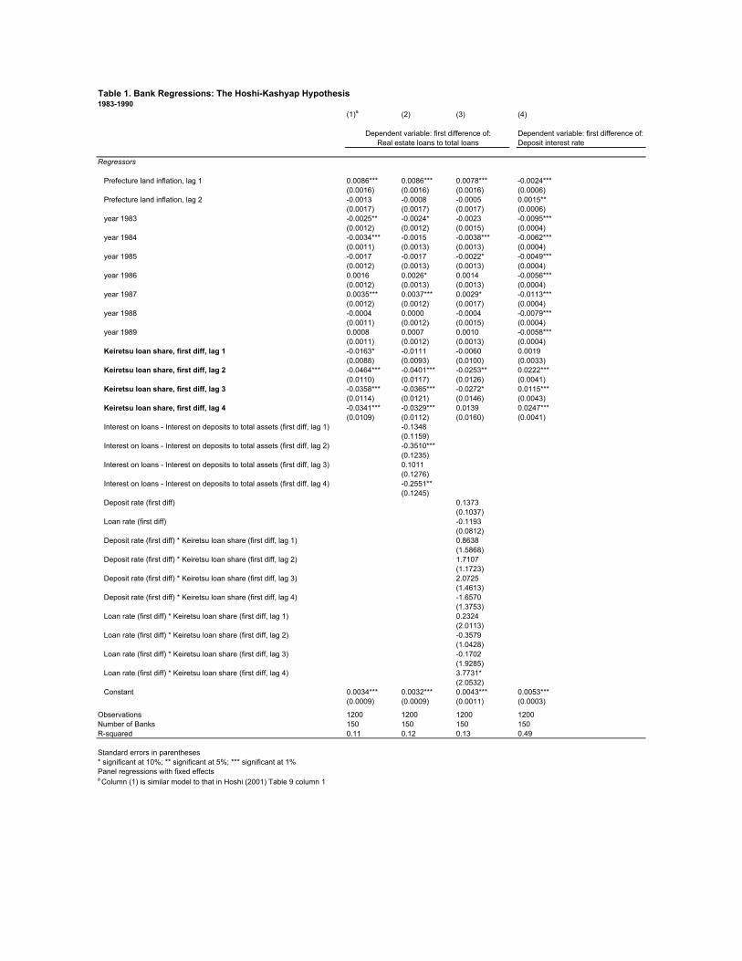
Table 1. Bank Regressions: The Hoshi-Kashyap Hypothesis1983-1990

(1)a (2) (3) (4)

Deposit interest rate

Regressors

Prefecture land inflation, lag 1 0.0086*** 0.0086*** 0.0078*** -0.0024***(0.0016) (0.0016) (0.0016) (0.0006)

Prefecture land inflation, lag 2 -0.0013 -0.0008 -0.0005 0.0015**(0.0017) (0.0017) (0.0017) (0.0006)

year 1983 -0.0025** -0.0024* -0.0023 -0.0095***(0.0012) (0.0012) (0.0015) (0.0004)

year 1984 -0.0034*** -0.0015 -0.0038*** -0.0062***(0.0011) (0.0013) (0.0013) (0.0004)

year 1985 -0.0017 -0.0017 -0.0022* -0.0049***(0.0012) (0.0013) (0.0013) (0.0004)

year 1986 0.0016 0.0026* 0.0014 -0.0056***(0.0012) (0.0013) (0.0013) (0.0004)

year 1987 0.0035*** 0.0037*** 0.0029* -0.0113***(0.0012) (0.0012) (0.0017) (0.0004)

year 1988 -0.0004 0.0000 -0.0004 -0.0079***(0.0011) (0.0012) (0.0015) (0.0004)

year 1989 0.0008 0.0007 0.0010 -0.0058***(0.0011) (0.0012) (0.0013) (0.0004)

Keiretsu loan share, first diff, lag 1 -0.0163* -0.0111 -0.0060 0.0019(0.0088) (0.0093) (0.0100) (0.0033)

Keiretsu loan share, first diff, lag 2 -0.0464*** -0.0401*** -0.0253** 0.0222***(0.0110) (0.0117) (0.0126) (0.0041)

Keiretsu loan share, first diff, lag 3 -0.0358*** -0.0365*** -0.0272* 0.0115***(0.0114) (0.0121) (0.0146) (0.0043)

Keiretsu loan share, first diff, lag 4 -0.0341*** -0.0329*** 0.0139 0.0247***(0.0109) (0.0112) (0.0160) (0.0041)

Interest on loans - Interest on deposits to total assets (first diff, lag 1) -0.1348(0.1159)

Interest on loans - Interest on deposits to total assets (first diff, lag 2) -0.3510***(0.1235)

Interest on loans - Interest on deposits to total assets (first diff, lag 3) 0.1011(0.1276)

Interest on loans - Interest on deposits to total assets (first diff, lag 4) -0.2551**(0.1245)

Deposit rate (first diff) 0.1373(0.1037)

Loan rate (first diff) -0.1193(0.0812)

Deposit rate (first diff) * Keiretsu loan share (first diff, lag 1) 0.8638(1.5868)

Deposit rate (first diff) * Keiretsu loan share (first diff, lag 2) 1.7107(1.1723)

Deposit rate (first diff) * Keiretsu loan share (first diff, lag 3) 2.0725(1.4613)

Deposit rate (first diff) * Keiretsu loan share (first diff, lag 4) -1.6570(1.3753)

Loan rate (first diff) * Keiretsu loan share (first diff, lag 1) 0.2324(2.0113)

Loan rate (first diff) * Keiretsu loan share (first diff, lag 2) -0.3579(1.0428)

Loan rate (first diff) * Keiretsu loan share (first diff, lag 3) -0.1702(1.9285)

Loan rate (first diff) * Keiretsu loan share (first diff, lag 4) 3.7731*(2.0532)

Constant 0.0034*** 0.0032*** 0.0043*** 0.0053***(0.0009) (0.0009) (0.0011) (0.0003)

Observations 1200 1200 1200 1200Number of Banks 150 150 150 150R-squared 0.11 0.12 0.13 0.49

Standard errors in parentheses* significant at 10%; ** significant at 5%; *** significant at 1%Panel regressions with fixed effectsa Column (1) is similar model to that in Hoshi (2001) Table 9 column 1

Real estate loans to total loansDependent variable: first difference of: Dependent variable: first difference of:

Table 2. Bond Issuance Eligibility for Domestic Secured Convertible Bondsa

1976 1977 1978 1979 1980 1981 1982 1983 1984 1985 1986 1987 1988 1989 1990

Number of companies eligible 65 378 422 496 559 616 671 675 727 799 819 855 1084 1247 1374

As a share of total companies (in %) 21.5 25.0 27.3 31.8 35.5 38.6 41.3 41.1 43.9 47.9 49.0 51.7 63.4 68.2 71.7

Source: Author's calculations based on the accounting criteria effective in Japan from October 1976-December 1990. These are given in Appendix Table 1.The underlying accounting data comes from the Development Bank of Japan Corporate Finance Data Set. Therefore "total companies" refers to the entiresample of companies with accounting data available in a given year.

aNote that convertible bonds were the principle source of public debt financing during the 1980s and these criteria were also applied to foreign issues of convertible bonds. Refer to Hoshi (1996).

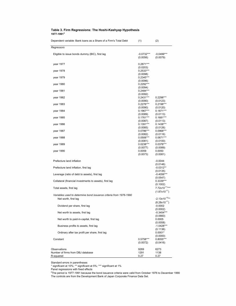
Table 3. Firm Regressions: The Hoshi-Kashyap Hypothesis1977-1991a

Dependent variable: Bank loans as a Share of a Firm's Total Debt (1) (2)

Regressors

Eligible to issue bonds dummy (BIC), first lag -0.0732*** -0.0499***(0.0056) (0.0079)

year 1977 0.2871***(0.0203)

year 1978 0.2533***(0.0098)

year 1979 0.2345***(0.0096)

year 1980 0.2292***(0.0094)

year 1981 0.2484***(0.0092)

year 1982 0.2431*** 0.2298***(0.0090) (0.0123)

year 1983 0.2276*** 0.2198***(0.0090) (0.0120)

year 1984 0.1967*** 0.1871***(0.0089) (0.0113)

year 1985 0.1761*** 0.1681***(0.0087) (0.0113)

year 1986 0.1391*** 0.1438***(0.0085) (0.0126)

year 1987 0.0786*** 0.0968***(0.0082) (0.0116)

year 1988 0.0506*** 0.0671***(0.0081) (0.0100)

year 1989 0.0238*** 0.0378***(0.0077) (0.0089)

year 1990 0.0059 0.0050(0.0073) (0.0081)

Prefecture land inflation -0.0044(0.0146)

Prefecture land inflation, first lag -0.0312**(0.0135)

Leverage (ratio of debt to assets), first lag -0.4056***(0.0547)

Collateral (financial investments to assets), first lag 0.3339***(0.1002)

Total assets, first lag 7.72x10-11***(1.87x10-11)

Variables used to determine bond issuance criteria from 1976-1990Net worth, first lag -2.13x10-10**

(8.28x10-11)Dividend per share, first lag -0.0002

(0.0002)Net worth to assets, first lag -0.3454***

(0.0660)Net worth to paid-in-capital, first lag 0.0005

(0.0058)Business profits to assets, first lag -1.0428***

(0.1136)Ordinary after tax profit per share, first lag 0.0001*

(0.0000)Constant 0.5758*** 0.8055***

(0.0072) (0.0416)

Observations 9269 6273Number of firms from DBJ database 1291 1138R-squared 0.27 0.27

Standard errors in parentheses* significant at 10%; ** significant at 5%; *** significant at 1%Panel regressions with fixed effectsaThe period is 1977-1991 because the bond issuance criteria were valid from October 1976 to December 1990The controls are from the Development Bank of Japan Corporate Finance Data Set.

Table 4. The Effect of Bank Credit on Land Prices: The Prefecture Cross-Sectional View

Dependent variable: Log difference in real prefectural (1) (2) (3) (4) (5) (6) (7) (8) land price between 1991 and 1981

All regressors are the difference between 1991 and 1981 a :

Keiretsu loan share -4.6568*** -3.4475***(0.7352) (0.9895)

Real estate loan share 11.4852*** 20.3016*** 14.8649***(2.1672) (4.6123) (4.8989)

"Risky" loan share (loans to real estate & construction & 4.4586** 14.2489*** 13.5435*non-bank financial institutions.) (1.6632) (5.0130) (7.5214)

Macro controls b

Prefecture population, in logs 3.6120*** 0.8910 3.8869*(0.9883) (1.3197) (2.1875)

Prefecture unemployment rate -0.1376 0.0878 0.0019(0.1940) (0.2183) (0.3484)

Prefecture income per capita, in logs -0.0994 1.1116 -2.9717(0.7785) (0.9088) (3.1228)

Prefecture job openings to applications -0.2670* -0.2694 -0.0069(0.1415) (0.1740) (0.3522)

Prefecture CPI excluding rent, in logs 0.3925 4.0841 -3.1615(3.3966) (2.7428) (8.1607)

Instrumenting for real estate or "risk" loan share with Yes Yes Yes Yeskeiretsu loan share?

Constant 0.8961*** 0.7439*** 0.5197*** 0.6749*** -0.1180 1.0232 -0.5199 1.8371(0.0547) (0.0641) (0.1180) (0.1252) (0.4103) (0.7128) (0.7229) (2.0110)

Number of prefectures 47 47 47 47 47 47 47 47R-squared 0.35 0.38 0.16 0.17 R-sq < 0b 0.57 0.46 R-sq < 0c

Robust standard errors in parentheses (clustered by prefecture)* significant at 10%; ** significant at 5%; *** significant at 1%aExcept for Prefecture population and unemployment which are the difference between 1990 and 1980 due to data availability.bThe controls are compiled from the Japan Statistical Yearbook, various issues.cNote that in 2SLS the R-squared can sometimes be negative, even when a constant is included.

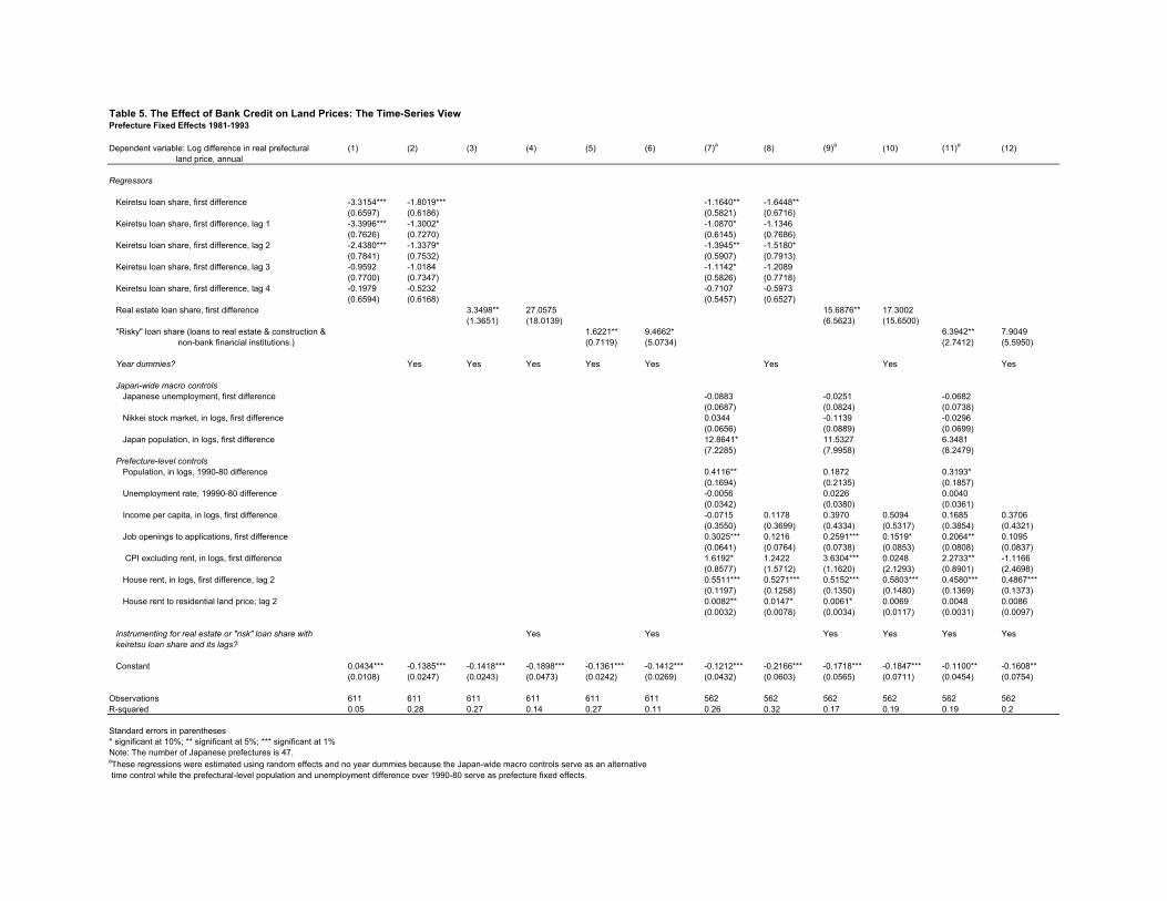
Table 5. The Effect of Bank Credit on Land Prices: The Time-Series ViewPrefecture Fixed Effects 1981-1993

Dependent variable: Log difference in real prefectural (1) (2) (3) (4) (5) (6) (7)a (8) (9)a (10) (11)a (12) land price, annual

Regressors

Keiretsu loan share, first difference -3.3154*** -1.8019*** -1.1640** -1.6448**(0.6597) (0.6186) (0.5821) (0.6716)

Keiretsu loan share, first difference, lag 1 -3.3996*** -1.3002* -1.0870* -1.1346(0.7626) (0.7270) (0.6145) (0.7686)

Keiretsu loan share, first difference, lag 2 -2.4380*** -1.3379* -1.3945** -1.5180*(0.7841) (0.7532) (0.5907) (0.7913)

Keiretsu loan share, first difference, lag 3 -0.9592 -1.0184 -1.1142* -1.2089(0.7700) (0.7347) (0.5826) (0.7718)

Keiretsu loan share, first difference, lag 4 -0.1979 -0.5232 -0.7107 -0.5973(0.6594) (0.6168) (0.5457) (0.6527)

Real estate loan share, first difference 3.3498** 27.0575 15.6876** 17.3002(1.3651) (18.0139) (6.5623) (15.6500)

"Risky" loan share (loans to real estate & construction & 1.6221** 9.4662* 6.3942** 7.9049non-bank financial institutions.) (0.7119) (5.0734) (2.7412) (5.5950)

Year dummies? Yes Yes Yes Yes Yes Yes Yes Yes

Japan-wide macro controlsJapanese unemployment, first difference -0.0883 -0.0251 -0.0682

(0.0687) (0.0824) (0.0738)Nikkei stock market, in logs, first difference 0.0344 -0.1139 -0.0296

(0.0656) (0.0889) (0.0699)Japan population, in logs, first difference 12.8641* 11.5327 6.3481

(7.2285) (7.9958) (8.2479)Prefecture-level controls

Population, in logs, 1990-80 difference 0.4116** 0.1872 0.3193*(0.1694) (0.2135) (0.1857)

Unemployment rate, 19990-80 difference -0.0056 0.0226 0.0040(0.0342) (0.0380) (0.0361)

Income per capita, in logs, first difference -0.0715 0.1178 0.3970 0.5094 0.1685 0.3706(0.3550) (0.3699) (0.4334) (0.5317) (0.3854) (0.4321)

Job openings to applications, first difference 0.3025*** 0.1216 0.2591*** 0.1519* 0.2064** 0.1095(0.0641) (0.0764) (0.0738) (0.0853) (0.0808) (0.0837)

CPI excluding rent, in logs, first difference 1.6192* 1.2422 3.6304*** 0.0248 2.2733** -1.1166(0.8577) (1.5712) (1.1620) (2.1293) (0.8901) (2.4698)

House rent, in logs, first difference, lag 2 0.5511*** 0.5271*** 0.5152*** 0.5803*** 0.4580*** 0.4867***(0.1197) (0.1258) (0.1350) (0.1480) (0.1369) (0.1373)

House rent to residential land price, lag 2 0.0082** 0.0147* 0.0061* 0.0069 0.0048 0.0086(0.0032) (0.0078) (0.0034) (0.0117) (0.0031) (0.0097)

Instrumenting for real estate or "risk" loan share with Yes Yes Yes Yes Yes Yeskeiretsu loan share and its lags?

Constant 0.0434*** -0.1385*** -0.1418*** -0.1898*** -0.1361*** -0.1412*** -0.1212*** -0.2166*** -0.1718*** -0.1847*** -0.1100** -0.1608**(0.0108) (0.0247) (0.0243) (0.0473) (0.0242) (0.0269) (0.0432) (0.0603) (0.0565) (0.0711) (0.0454) (0.0754)

Observations 611 611 611 611 611 611 562 562 562 562 562 562R-squared 0.05 0.28 0.27 0.14 0.27 0.11 0.26 0.32 0.17 0.19 0.19 0.2

Standard errors in parentheses* significant at 10%; ** significant at 5%; *** significant at 1%Note: The number of Japanese prefectures is 47.aThese regressions were estimated using random effects and no year dummies because the Japan-wide macro controls serve as an alternative time control while the prefectural-level population and unemployment difference over 1990-80 serve as prefecture fixed effects.

Appendix Table 1. Bond Issuance Criteria for Domestic Secured Convertible Bonds

Effective October 1976 - July 1987

A firm with net worth greater than 10 billion yen can issue if: 1. Dividend per share in the most recent accounting period exceeds 5 yen and2. Ordinary after-tax profit per share in the most recent accounting period is greater than 7 yen and3. One of the following 3 conditions is met:

a. Net worth ratio is greater than or equal to 0.15b. Net worth / paid-in-capital is greater than or equal to 1.2c. Business profits / total assets is greater than or equal to 0.04

A firm with net worth greater than 6 billion yen but less than 10 billion yen can issue if: 1. Dividend per share in the most recent accounting period exceeds 5 yen and2. Ordinary after-tax profit per share in the most recent accounting period is greater than 7 yen and3. Two of the following 3 conditions are met:

a. Net worth ratio is greater than or equal to 0.2b. Net worth / paid-in-capital is greater than or equal to 1.5c. Business profits / total assets is greater than or equal to 0.05

Effective July 1987 - December 1990a

A firm with net worth greater than 10 billion yen can issue if: 1. Dividend per share in the most recent accounting period exceeds 5 yen and2. Ordinary after-tax profit per share in the most recent accounting period is greater than 7 yen and3. One of the following 3 conditions is met:

a. Net worth ratio is greater than or equal to 0.1b. Net worth / paid-in-capital is greater than or equal to 1.2c. Business profits / total assets is greater than or equal to 0.05

A firm with net worth greater than 6 billion yen but less than 10 billion yen can issue if: 1. Dividend per share in the most recent accounting period exceeds 5 yen and2. Ordinary after-tax profit per share in the most recent accounting period is greater than 7 yen and3. Two of the following 3 conditions are met:

a. Net worth ratio is greater than or equal to 0.12b. Net worth / paid-in-capital is greater than or equal to 1.5c. Business profits / total assets is greater than or equal to 0.06

A firm with net worth greater than 3 billion yen but less than 6 billion yen can issue if: 1. Dividend per share in the most recent accounting period exceeds 5 yen and2. Ordinary after-tax profit per share in the most recent accounting period is greater than 7 yen and3. Two of the following 3 conditions are met:

a. Net worth ratio is greater than or equal to 0.15b. Net worth / paid-in-capital is greater than or equal to 2.0c. Business profits / total assets is greater than or equal to 0.07

Source: Hoshi, Kashyap and Scharfstein (1993).a Rating criteria became effective from May 1989 whereby a firm wih a BB rating or higher could issue bonds if

its dividend per share were greater than 5 yen and its ordinary after-tax profit per share were greater than 7 yen.After December 1990, the accounting criteria ceased to be in effect and only the rating criteria were applicable.Therefore for the period May 1989-December 1990, the eligible-to-issue firms tabulated in Table 2 and based on only the accounting criteria are biased downwards.

Figure 1. Keiretsu and Real Estate Loans, All banks (average)

Figure 1a. Keiretsu Loans and Loans to Listed Firms (as a share of total loans)

Figure 1b. Proportion of Loans to the Real Estate Sector

Source: The keiretsu loans and loans to listed firms were provided by Takeo Hoshi,who compiled them from Keizai Chosakai, Kin'yu Kikan no Toyushi (Investment and Loans by Financial Institutions), various issues.The real estate loans and the total loans come from the Nikkei NEEDS database.

.05

.1.1

5.2

1975 1980 1985 1990 1995 2000

Loans to keiretsu Loans to listed

.06

.07

.08

.09

.1.1

1

1975 1980 1985 1990 1995 2000

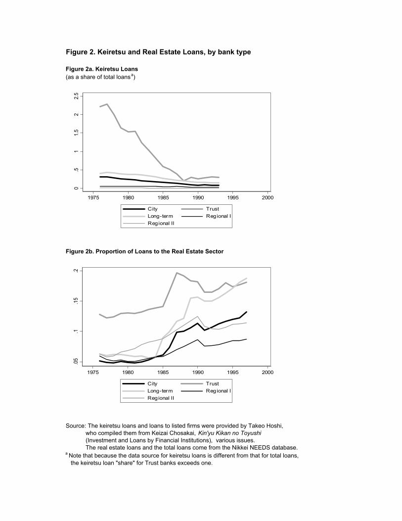
Figure 2. Keiretsu and Real Estate Loans, by bank type

Figure 2a. Keiretsu Loans (as a share of total loansa)

Figure 2b. Proportion of Loans to the Real Estate Sector

Source: The keiretsu loans and loans to listed firms were provided by Takeo Hoshi,who compiled them from Keizai Chosakai, Kin'yu Kikan no Toyushi (Investment and Loans by Financial Institutions), various issues.The real estate loans and the total loans come from the Nikkei NEEDS database.

a Note that because the data source for keiretsu loans is different from that for total loans, the keiretsu loan "share" for Trust banks exceeds one.

0.5

11.

52

2.5

1975 1980 1985 1990 1995 2000

City TrustLong-term Regional IRegional II

.05

.1.1

5.2

1975 1980 1985 1990 1995 2000

City TrustLong-term Reg ional IRegional II

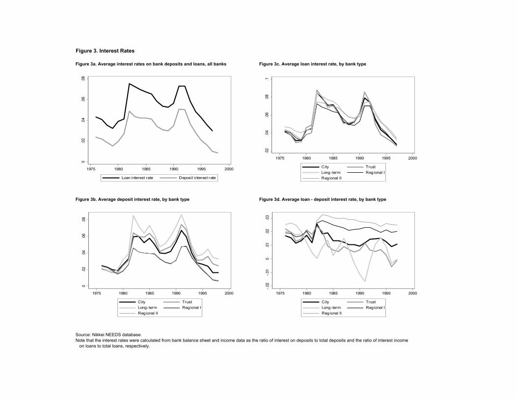
Figure 3. Interest Rates

Figure 3a. Average interest rates on bank deposits and loans, all banks Figure 3c. Average loan interest rate, by bank type

Figure 3b. Average deposit interest rate, by bank type Figure 3d. Average loan - deposit interest rate, by bank type

Source: Nikkei NEEDS database.Note that the interest rates were calculated from bank balance sheet and income data as the ratio of interest on deposits to total deposits and the ratio of interest income

on loans to total loans, respectively.

0.0

2.0

4.0

6.0

8

1975 1980 1985 1990 1995 2000

Loan interest rate Deposit interest rate

-.02

-.01

0.0

1.0

2.0

3

1975 1980 1985 1990 1995 2000

City TrustLong-term Regional IRegional II

.02

.04

.06

.08

.1

1975 1980 1985 1990 1995 2000

City TrustLong-term Reg ional IRegional II

0.0

2.0

4.0

6.0

8

1975 1980 1985 1990 1995 2000

City TrustLong-term Regional IRegional II

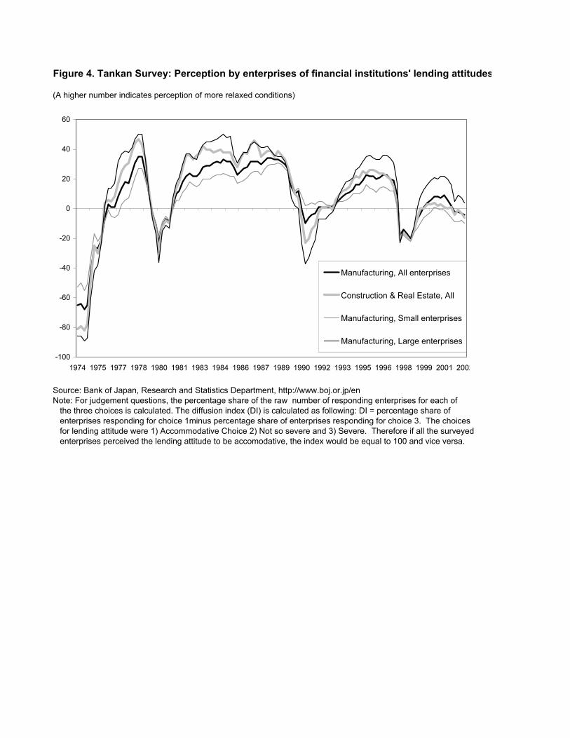
Figure 4. Tankan Survey: Perception by enterprises of financial institutions' lending attitudes

(A higher number indicates perception of more relaxed conditions)

Source: Bank of Japan, Research and Statistics Department, http://www.boj.or.jp/enNote: For judgement questions, the percentage share of the raw number of responding enterprises for each of

the three choices is calculated. The diffusion index (DI) is calculated as following: DI = percentage share of enterprises responding for choice 1minus percentage share of enterprises responding for choice 3. The choices for lending attitude were 1) Accommodative Choice 2) Not so severe and 3) Severe. Therefore if all the surveyed enterprises perceived the lending attitude to be accomodative, the index would be equal to 100 and vice versa.

-100

-80

-60

-40

-20

0

20

40

60

1974 1975 1977 1978 1980 1981 1983 1984 1986 1987 1989 1990 1992 1993 1995 1996 1998 1999 2001 2002

Manufacturing, All enterprises

Construction & Real Estate, All

Manufacturing, Small enterprises

Manufacturing, Large enterprises

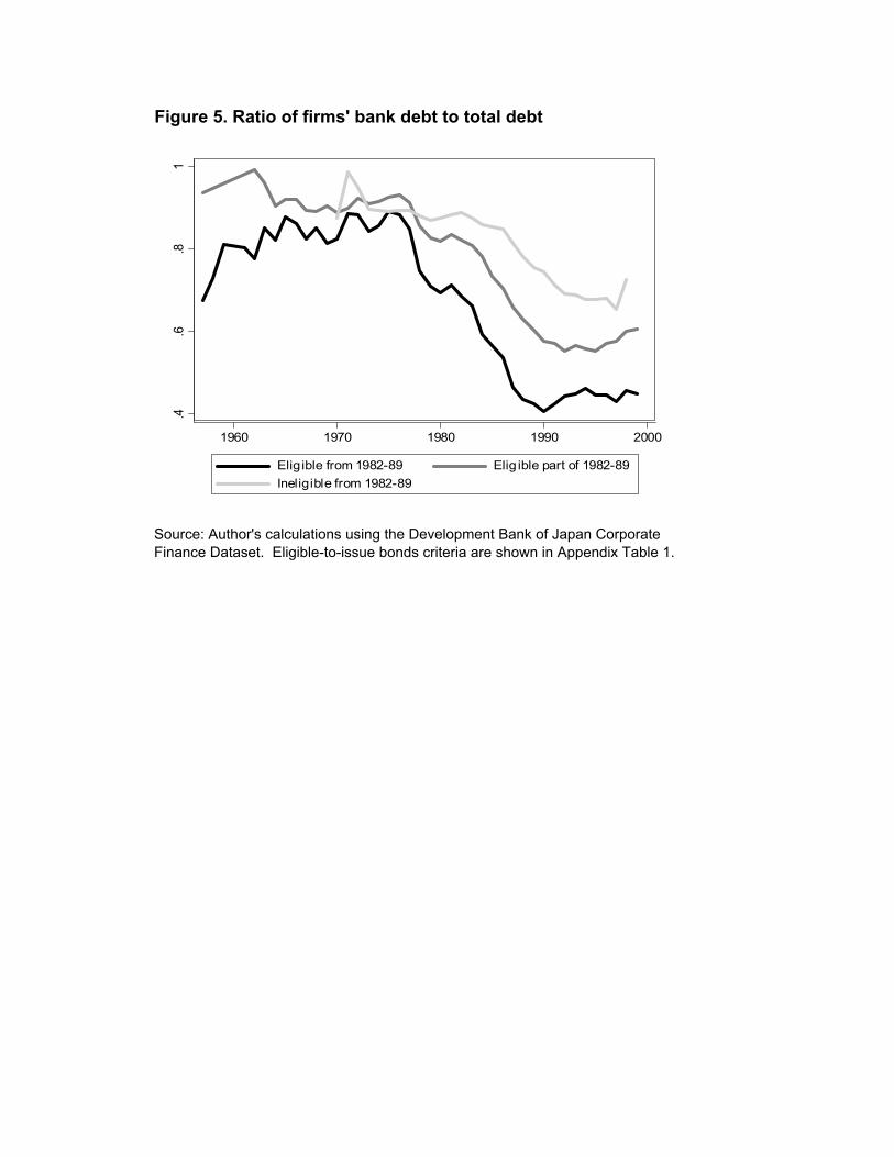
Figure 5. Ratio of firms' bank debt to total debt

Source: Author's calculations using the Development Bank of Japan CorporateFinance Dataset. Eligible-to-issue bonds criteria are shown in Appendix Table 1.

.4.6

.81

1960 1970 1980 1990 2000

Elig ible from 1982-89 Elig ible part of 1982-89Ineligible from 1982-89

Figure 6. Inflation

Figure 6a. Land price inflation and the Nikkei stock market index

Figure 6b. Prefecture-level land price inflation (selected prefectures)

Source: Nikkei stock market index from Bank of Japan, http://www.boj.or.jp/enLand prices, all areas and 6 largest cities are from the Japan Statistical Yearbook's Table 17-12 Index of Urban Land Prices (1960-2003), which in turn are from the Japan Real Estate Institute (as of end-March).Prefecture land prices are from the Japan Statistical Yearbook, various issues, which come fromthe annual July 1st Prefectural Land Price Survey carried out by the Land and Water Bureau, Ministry of Land, Infrastructure and Transport. The weighted average over 6 categories of land is taken: residential site, prospective housing land, commercial site, quasi-industrial site, industrial site, and housing land within urbanization control area. Land price indices are divided by the GDP deflator to obtain real land prices, then the inflation rate iscalculated as the annual log difference.

-.4-.2

-5.5

5e-1

7.2

.4

1975 1980 1985 1990 1995 2000

Land price inflation, 6 largest cities Land price inflation, all areasNikkei index, % change

-.50

.51

1975 1980 1985 1990 1995 2000

Tokyo OsakaHokkaido Okinawa

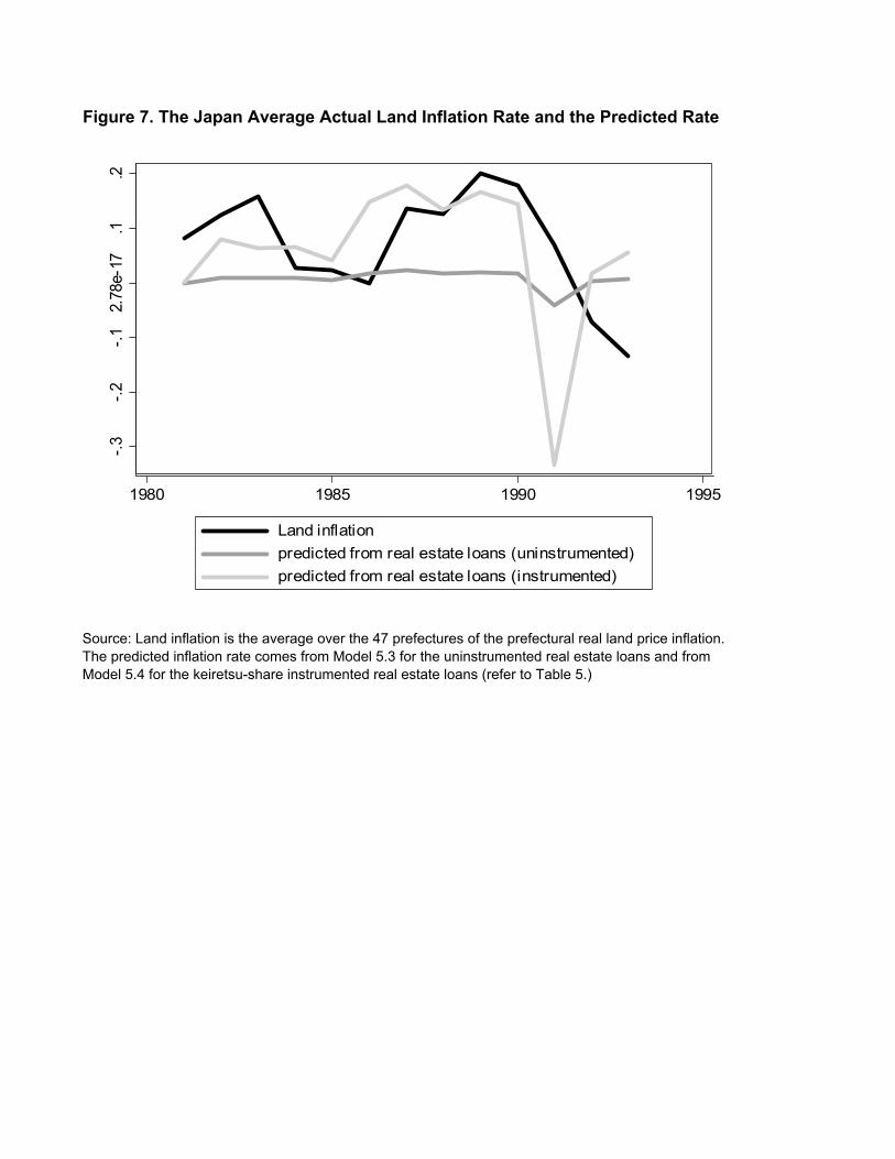
Figure 7. The Japan Average Actual Land Inflation Rate and the Predicted Rate

Source: Land inflation is the average over the 47 prefectures of the prefectural real land price inflation.The predicted inflation rate comes from Model 5.3 for the uninstrumented real estate loans and fromModel 5.4 for the keiretsu-share instrumented real estate loans (refer to Table 5.)

-.3-.2

-.12.

78e-

17.1

.2

1980 1985 1990 1995

Land inflationpredicted from real estate loans (uninstrumented)predicted from real estate loans (instrumented)