The Economy of People’s Republic of China from 1953∗

Anton Cheremukhin, Mikhail Golosov, Sergei Guriev, Aleh Tsyvinski

July 27, 2015

Abstract

We study growth and structural transformation of China in the pre-1978 and post-1978periods in a unified framework. First, we construct a dataset that allows the applicationof the neoclassical model with wedges. Second, we show that changes in the intersectorallabor wedge play a dominant role in reallocation of labor from agriculture and, togetherwith TFP growth, in GDP growth. The production component (the gap between the ratioof the marginal products of labor and relative wages) and the consumption component (thegap between the marginal rate of substitution and the relative prices) play a particularlyimportant role. Third, we use the pre-1978 reform period as a benchmark to measure thesuccess of the reforms. We provide historical evidence that the decrease in the productioncomponent is consistent with demonopolization of the economy and that the decrease inthe consumption component is consistent with the price and housing reforms.

∗Cheremukhin: Federal Reserve Bank of Dallas; Golosov: Princeton and NES; Guriev: Sciences Po, Paris;Tsyvinski: Yale. We are indebted to Carsten Holz for providing us with several data series in this paperand for his many insightful discussions on Chinese statistics. We also thank Andrew Atkeson, Loren Brandt,Francisco Buera, Ariel Burstein, Brent Neiman, Lee Ohanian, Nancy Qian, Stephen Roach, Michael Song, KjetilStoresletten, Xiaodong Zhu, and Fabrizio Zilibotti for their comments; Yukun Liu, Stefano Malfitano and KaiYan for research assistance; and audiences at Chicago Fed, Chicago Booth, Toronto, Harvard, Tsinghua Centerfor Growth and Institutions, Tsinghua Macro Conference, NBER Summer Institute (Development Economicsand Economic Fluctuations and Growth), Bank of Canada-University of Toronto Conference on the ChineseEconomy, Joint French Macro Workshop, Facsem at Sciences Po, EEA Annual Meeting in Toulouse. Financialassistance from Banque de France is gratefully acknowledged. Any opinions, findings or recommendationsexpressed in this paper are those of the authors and do not necessarily reflect the views of their colleagues,affiliated organizations, Banque de France, the Federal Reserve Bank of Dallas or the Federal Reserve System.

1 Introduction

We study the Chinese economy from 1953, three years after the founding of the People’s Re-

public of China, through the lens of a two-sector neoclassical growth model.1 Our main focus

is on studying wedges that hinder reallocation of resources across sectors and the changes of

these wedges that are important for structural transformation.2 The main goal of the paper is

to provide a systematic analysis of both the pre-1978 reform and the post-reform periods in a

unified framework.

Specifically, our model is a two-sector (agricultural and non-agricultural) neoclassical model

with wedges building on Cole and Ohanian (2004), Chari, Kehoe, McGrattan (2007) and Chere-

mukhin, Golosov, Guriev, and Tsyvinski (2013). The intratemporal labor wedge is the cost of

intersectoral reallocation of labor. The intratemporal capital wedge is the cost of intersec-

toral reallocation of capital. The intertemporal capital wedge is the cost of reallocating capital

across time. We further decompose the intersectoral labor wedge in three components: the

consumption component (the ratio of the relative prices and the marginal rate of substitution),

the production component (the ratio of the sectoral marginal products of labor relative to the

sectoral wages), and the mobility component (the ratio of the sectoral wages). We similarly

decompose the intersectoral capital wedge into its components.

We construct a comprehensive dataset that allows the application of the neoclassical model

to the study of the entire 1953-2012 period. We provide consistent data series for sectoral

output, capital and labor, wages, deflators, and relative prices as well as defense spending and

international trade variables. Using this dataset we then infer the wedges (and other variables

such as sectoral TFPs) from the computed first order conditions of the model. Given the

wedges, the neoclassical model matches the data exactly. We view the construction of the

dataset that can be easily used for computations of the neoclassical model and for inferring the

wedges and their components for China as the first contribution of the paper.

We start our analysis with the pre-1978 reform economy. This period is important to study

for several reasons. First, 1953-1978 was one of the largest economic policy experiments and1Our analysis takes as an initial point the year of 1953 — after the Communist Party consolidated power

and launched a comprehensive modernization of economy and society. Coincidentally, this is also the start ofthe systematic collection of detailed economic statistics.

2See Acemoglu (2008) and Herrendorf, Rogerson and Valentinyi (2013) for overview of the models of structuraltransformation. Caselli and Coleman (2001), Fernald and Neiman (2010), Restuccia, Yang and Zhu (2008), andLagakos and Waugh (2013) are the models with sector-specific wedges.

1

development programs in modern history. It is important to evaluate the overall success or

failure of this program as well as successes and failures of the contributing factors and policies.

Second, the analysis of the 1953-1978 period is an important benchmark against which the

post-1978 growth and the success of the reforms should be measured. The main question here

is how the Chinese economy would have developed if the pre-reform policies continued. Thirdly,

the successful First Five-Year Plan (FFYP), the Great Leap Forward (GLF), and the post-1962

period of readjustment, recovery, and political turmoil provide a range of interesting policies

on their own.

The first part of the analysis is to perform a wedge-accounting exercise for the entire pre-

reform period to determine the main factors behind GDP growth and changes in the share of

labor force in agriculture. We fix wedges at their initial values (1953) for the whole period of in-

terest (1953-75) and simulate the economy3. We then compare the simulated GDP growth and

the change in the share of labor force in agriculture with the actual historical paths. Compared

with the counterfactual, the annual growth rate of GDP increased by 5.6 percentage points and

the share of labor force in agriculture decreased by 5.9 percentage points. For GDP growth, the

two most important factors were the growth of non-agricultural TFP (contributing 1.9 percent-

age points) and the decrease in the consumption component of the labor wedge (contributing

1.6 percentage points). The rest of the wedges worsened and contributed negatively to the

growth of GDP. Overall, the worsening of wedges resulted in 0.5 percentage points reduction

in annual GDP growth. The change in the share of labor force in agriculture (-5.9 percentage

points) is essentially fully determined by the decrease in the consumption component of the

labor wedge (contributing -7.8 percentage points). While these are the numbers for the pre-

reform period overall, changes in the intersectoral labor wedge played an even more significant

role in GDP growth and changes in the share of labor force in agriculture during the Great

Leap Forward and the subsequent recovery.

We then contrast the development of the Chinese economy from the beginning of the Great

Leap Forward to 1967 with the development of the Soviet economy under Stalin’s industrial-

ization. On one hand, the model of Chinese development was based on Soviet Industrialization

which we studied in Cheremukhin, et al. (2013). On the other hand, the Chinese policies were3The analysis for 1953-1978 delivers similar insights and only differs in a larger change in the share of labor

in agriculture in 1975-1978.

2

quite distinct from their Soviet counterparts. We show that if China followed Soviet industri-

alization and collectivization policies the results in terms of GDP growth would be comparable

to a combination of the Great Leap Forward and the post-1962 retrenchment but the share of

labor force in agriculture would have been lower under Soviet policies. The quick reversal of

the policies under the Great Leap Forward led to a significantly higher labor wedge in China

but coincided with the recovery of the losses in agricultural and non-agricultural TFP.

We then study the 1978-2012 period through the lens of our model. We first perform a

wedge-accounting exercise for the period of 1978-2012. Compared with the counterfactual of

fixed 1978 wedges and no TFP growth, the annual GDP growth rate increased by 9.4 per-

centage points and the share of labor force in agriculture decreased by 36.9 percentage points.

For GDP growth, two most important factors were the growth of non-agricultural TFP (con-

tributing 5.8 percentage points) and the decrease in the intersectoral wedge (contributing 1.1

percentage points). Agricultural TFP contributed 0.8 percentage points. Two components of

the labor wedge played the key role – the decrease in the consumption component (contribut-

ing 0.5 percentage points) and the production component (contributing 0.7 percentage points).

Together these two components account for 1.2 percentage points of annual GDP growth. The

change in the mobility component of the intersectoral labor wedge, the intersectoral capital

wedge net of consumption component, and intertemporal capital wedge play a minor role. The

change in the share of labor in agriculture is predominantly determined by the decrease in the

intersectoral wedges (contributing -21.6 percentage points). Two components play the key role

– the consumption component (contributing -10.6 percentage points) and the production com-

ponent (contributing -16.7 percentage points). These two components play the same role as the

increase in manufacturing TFP (contributing -10.6 percentage points) and agricultural TFP

(contributing -12.2 percentage points). The worsening in the mobility component accounted

for 6.7 percentage points of the change in the share of labor force in agriculture. We conclude

that more than 50 percent of the GDP growth is explained by growth of non-agricultural TFP

and 11 percent are explained by the decline in the consumption and the production component

of the intersectoral wedges. The key factors behind the change in the share of labor force in

agriculture are the reduction in intersectoral wedges and TFP growth in equal measures.

Second, we simulate the continuation of the trends of the post-GLF (1967-1975) policies

for the post-1978 period to provide a benchmark against which to measure the success of the

3

post-1978 reforms. The reforms generate 4.2 additional percentage points of GDP growth. The

main factors are the faster growth of non-agricultural TFP (4.4 versus 2.0 percentage points)

that generates 3 percentage points of GDP growth and the faster decrease in the intersectoral

wedges that generates 1 percentage point of additional GDP growth. The dominant factors in

the decrease in the share of labor force in agriculture (-23.9 percentage points) are the decrease

in the production component of the labor wedge (contributing -14 percentage points) and the

faster manufacturing TFP growth (contributing -6.9 percentage points). We conclude that the

reforms yielded significant growth and structural transformation differentials compared with

the continuation of the post-GLF trends. In other words, about 3/4 of the growth differential

is due to the increased growth of the non-agricultural TFP; 1/4 of the growth differential is due

to the faster reduction in the intersectoral wedges. The reduction in the production component

of the labor wedge and growth in non-agricultural TFP are also dominant forces behind the

change in the share of labor force in agriculture.

We then provide extensive historical evidence consistent with the behavior of the wedges

through the lens of model for 1953-2012. Most importantly, we argue that the reforms that are

consistent with the changes in the key components of the intersectoral wedges post-1978 are:

the price and housing reform (for the consumption component), and the increase in competition

(for the production component).

We now briefly discuss the literature on the topic. A body of work by Carsten Holz is

the most comprehensive attempt to construct high-quality data for the analysis of China’s

economy: Holz (2006) assesses availability and quality of the data and constructs a number

of key data series for the analysis of productivity growth in 1952-2005; Holz (2013a) provides

a detailed guide to classification systems and data sources of Chinese statistics; Holz (2003,

2013b) studies the quality of China’s output statistics. Despite the importance of the issue,

there are no studies of the 1953-1978 period that use modern macroeconomic tools. Ours is the

first paper that analyzes this period from the point of view of the neoclassical growth model,

and provides a unified treatment of the Chinese economy from 1953 to 2012. We are aware of

only one strand of papers dedicated to model-based macroeconomic analysis of the 1953-1978

period by Chow (1985, 1993) and Chow and Li (2002) whose work mainly focuses on data

issues. The post-1978 period received more attention from macroeconomists but perhaps less

prominence than its importance would suggest. Notable contributions are a collection of papers

4

in a landmark book edited by Brandt and Rawski (2008), an important quantitative analysis of

China’s post-1978 structural transformation and sectoral growth accounting by Brandt, Hsieh,

and Zhu (2008), Brandt and Zhu (2010) and Dekle and Vandenbroucke (2010, 2012), growth

accounting by Young (2003) and Zhu (2012), the model of “growing like China” with the focus

on financial frictions by Song, Storesletten, and Zilibotti (2011), a study of misallocation by

Hsieh and Klenow (2010), analysis of factor wedges across space and sectors of Brandt, Tombe,

and Zhu (2013) and Tombe and Zhu (2015), a model of transformation of the state-owned firms

by Hsieh and Song (2015).

It is useful to also compare our post-1978 results with Brandt, Hsieh, and Zhu (2008), Brandt

and Zhu (2010) and Dekle and Vandenbroucke (2012) who study structural transformation of

China post-1978 reforms. They find that the decrease in the barrier to labor reallocation played

a relatively small role in the change in the share of labor force in agriculture. The key difference

is that their notion of the barrier captures only a part of the labor wedge (that corresponds to

our production and mobility components of the wedge but omits the consumption component).

When the reduction in the overall wedge is taken into account, as we do here, the contribution

of this factor more than doubles. We further compare our results by extending our model

to a three-sector version where we divide the non-agricultural sector into the state- and the

non-state sector following Brandt and Zhu (2010). We then decompose the contribution of non-

agricultural TFP to the structural transformation in 1978-2012 into the contributions of TFP

growth in the state- and non-state sectors, respectively, and the contribution of reallocation

from the less productive state sector to the more productive non-state sector. We confirm the

findings of Brandt, Hsieh, and Zhu (2008) and Brandt and Zhu (2010) of the importance of

growth of non-state TFP in overall TFP growth. We also in passing note that our model with

wedges (by construction) matches the data exactly while these papers rely on calibration to

match some (but not all) features of the data.

More broadly, our paper is related to such studies of structural transformation as Caselli

and Coleman (2001), Kongsamut, Rebelo and Xie (2001), Stokey (2001), Ngai and Pissarides

(2007), Hayashi and Prescott (2008), Acemoglu and Guerreri (2008), Buera and Kaboski (2009,

2012), Herrendorf, Rogerson and Valentinyi (2013). The main difference with this literature is

that we find that the changes in the intersectoral labor wedges (and policies associated with

them) play an important role in structural transformation. Also notable is a two-sector model

5

of growth accounting with misallocation applied to Singapore by Fernald and Neiman (2010).

2 Model

We consider a two-sector (agricultural (A) and non-agricultural (M)) neoclassical model that

we used to analyze Stalin’s industrialization (Cheremukhin et al., 2013).

The preferences are given by:

∞∑t=0

βtU(CAt , C

Mt

)1−ρ − 1

1− ρ, (1)

where

U(CAt , C

Mt

)=

[η

1σ(CAt − γA

)σ−1σ + (1− η)

1σ(CMt

)σ−1σ

] σσ−1

,

CAt and CMt are per capita consumption of, respectively, agricultural and non-agricultural

goods; γA ≥ 0 is the subsistence level of consumption of agricultural goods; η is the long-run

share of agricultural expenditure in consumption; Ui,t is the marginal utility with respect to

consumption of good i in period t. The discount factor is β ∈ (0, 1), and σ is the elasticity

of substitution between the two consumption goods. Each agent is endowed with one unit of

labor services that he supplies inelastically.

Output in sector i ∈ {A,M} is given by:

Y it = F it

(Kit , N

it

)= Xi

t

(Kit

)αK,i (N it

)αN,i , (2)

where Xit , K

it , and N i

t are, respectively, total factor productivity, capital stock, and labor in

sector i. The capital and labor shares αK,i and αN,i satisfy αK,i + αN,i ≤ 1. Land is available

in fixed supply, and its share in production in sector i is 1 − αK,i − αN,i. We denote by F iK,tand F iN,t the derivatives of F it with respect to Ki

t and N it .

The total population in period t is denoted by Nt, and is exogenous. The feasibility con-

straint for labor is

NAt +NM

t = χtNt, (3)

where χt is an exogenously given fraction of working age population.

New capital It can be produced only in the non-agricultural sector. The aggregate capital

stock satisfies the law of motion

Kt+1 = It + (1− δ)Kt, (4)

6

where δ is the depreciation rate. Denoting by KAt and KM

t the capital stock in agriculture and

manufacturing, the feasibility condition for intersectoral capital allocation is

KAt +KM

t = Kt. (5)

Net exports of agricultural and manufacturing goods, EMt and EAt , and government ex-

penditures on manufacturing goods, GMt , are exogenous. The feasibility conditions in the two

sectors are

NtCAt + EAt = Y A

t , (6)

and

NtCMt + It +GMt + EMt = YM

t . (7)

The efficient allocations in this economy satisfy three first order conditions: the intra-

temporal labor allocation condition across sectors:

1 =UM,t

UA,t

FMN,t

FAN,t, (8)

the intra-temporal capital allocation condition across sectors:

1 =UM,t

UA,t

FMK,t

FAK,t, (9)

and the inter-temporal condition:

1 =(1 + FMK,t+1 − δ

)βUM,t+1

UM,t. (10)

Following Chari, Kehoe and McGrattan (2007), we define three wedges 1 + τW,t, 1 + τR,t,

and 1 + τK,t as the right hand sides of expressions (8), (9), and (10). We note that our analysis

is an accounting procedure as competitive general equilibrium allocations with wedges match

data exactly.

We also study the components of the wedges. Let pi,t and wi,t denote the prices of goods

and wages in the competitive equilibrium. The right hand side of the intra-temporal optimality

condition for labor (8) can be re-written as a product of three terms, to which we refer as

consumption, production, and labor mobility components:

UM,t

UA,t

FMN,t

FAN,t=

UM,t/pM,t

UA,t/pA,t︸ ︷︷ ︸consumption component

×pM,tF

MN,t/wM,t

pA,tFAN,t/wA,t︸ ︷︷ ︸production component

×wM,t

wA,t︸ ︷︷ ︸labor mobility component

. (11)

7

In the competitive equilibrium decentralizing the efficient allocation, all three components are

equal to one. Each of these components is an optimality condition in one of the three markets.

The first, consumption, component is the optimality condition of consumers. The consumption

component typically measures frictions in consumer goods markets. The second, production,

component is the optimality condition of competitive, price-taking firms. The production

component measures frictions in the production process such as monopoly power. The third,

mobility, component is equal to one when workers can freely choose in which sector to work. The

mobility component measures frictions in labor allocation between sectors, conditional on the

relative wages. An analogous decomposition can be done for the intersectoral capital wedge (9).

As we do not have reliable data on interest rates in each sector, we decompose the intratemporal

capital wedge only into two components, consumption and non-consumption components. Note

that the consumption component is common for the labor and capital wedges.

3 Data

In this section we discuss the construction of the data for a systematic analysis of the structural

transformation of the Chinese economy from 1952 to 2012.4 One contribution of our paper is

construction of the data for an application of a two-sector neoclassical model for this period.

3.1 Data sources and construction of the data

Our two main sources of data on China national accounts are the yearly “China Statistical

Yearbooks” (CSY) and the “60 Years of New China” (60Y). Both sources are published by the

Chinese National Bureau of Statistics (NBS). The second source aggregates data from previous

publications for the years 1949-2009 and is also closely related with a book on pre-1996 statistics

compiled by Hsueh and Li (1999), “China’s national income 1952-1995” (HL).

We use nominal value added by sector and the growth rate of real value added by sector

to construct indices of real value added in the agricultural (primary) sector and the non-

agricultural (secondary and tertiary) sector in 1978 prices. The same sources allow us to

estimate the relative prices of agricultural goods to non-agricultural goods by taking the ratio

of price deflators in the two sectors. The price deflator in each sector is computed as the ratio

of nominal to real value added in that sector. The ratio of price deflators equals 1 in 19784The detailed data series are provided in the working paper Cheremukhin et al. (2015).

8

by construction. We use gross fixed capital formation in current prices which serves as our

measure of nominal investment. We convert investment (as well as other components of GDP)

from nominal to real values using the GDP deflator.

We use Holz (2006), Tables 19 and 20 on pages 159-161, as our main source for the aggregate

and sectoral capital stock. We use the level of capital and its ratio to GDP in 1953 to estimate

the initial level of capital in 1978 prices. We apply the perpetual inventory method (with a

depreciation rate of 5 percent) to our series for real investment in 1978 prices to obtain the

series for aggregate capital in 1978 prices. The series that we obtain is largely consistent with

Holz’s estimates of aggregate capital stock for 1953-2006, with two minor differences: Holz

computes capital in constant 2000 prices and uses a variable depreciation rate which ranges

between 3 and 5 percent.

We also use data from Holz (2006) to divide the aggregate capital stock into capital used

in the agricultural and non-agricultural sectors. This sectoral division of capital stock is only

available for 1978-2012. For earlier years we use the data on sectoral investment from Chow

(1993) to estimate the composition of capital stock by sector. We use net capital stock accu-

mulation by sector from Table 5 on page 820 in Chow (1993), and then apply the perpetual

inventory method to accumulate sectoral capital stock for 1953-1978. We break down the total

real capital stock in 1978 prices by sector using the relative proportions implied by Chow’s

data. We also constructed data on sectoral capital stock using provincial data for the pre-1978

period and the results are consistent with our main series.

For labor input, we use data on population, employment and its composition from the

two primary sources (60Y, CSY). We adjust the employment numbers prior to 1990 using the

procedure proposed by Holz (2006), Appendix 13, page 236. The correction addresses the

reclassification of employed workers that was made by the NBS in 1990.

For data on wages by sector we use average wages for staff and workers in the agricultural

and non-agricultural sectors for 1952-2012. The pre-1978 data come from CSY for year 1981.

The post-1978 data come from CSY for years 1996-2013. One issue with this data is that the

wages of staff and workers may not be the same as labor remuneration for workers. Staff and

workers are concentrated in non-agriculture, and to the extent that they are in agriculture, they

are likely in state farms5. We address this concern by computing the ratio of labor remuneration5See, for example, Holz (2014) for detailed data.

9

in non-agriculture to agriculture from Bai and Qian (2010). We find that the ratio of two series

behaves similarly for the overlapping time period (see Online Data Appendix for more details).

Our primary source of data on sectoral price indexes is the CSY. We use sectoral value

added deflators obtained earlier when computing real value added by sector.

The data on defense spending comes from three main sources. The earlier period of 1952-

1995 is jointly covered by HL and CSY, which report nominal defense spending in yuan. For

the period 1983-2012 an alternative source of data is the website of the Stockholm International

Peace Research Institute (SIPRI) which reports spending on defense for a variety of countries

as a percent of GDP. For the overlapping period the trends are broadly consistent but the exact

estimates vary by a factor of 1 to 1.5. As there seems to be no reliable way of obtaining more

precise estimates, we average the two available sources for the overlapping period. We obtain

an estimate of real defense spending in 1978 prices using the share of defense in GDP from

these two sources.

The main source for data on sectoral exports and imports is Fukao, Kiyota and Yue (2006).

Fukao et al. report data on China’s exports and imports by commodity at the SITC-R 2-digit

level for 1952-1964 and for 1981-2000, obtained from the “China’s Long-Term International

Trade Statistics” database. Using data from Fukao et al. (2006), we construct estimates

of nominal exports and imports of agricultural and non-agricultural commodities. We then

subtract imports from exports to obtain estimates of net exports by sector. We use the price

deflators computed earlier to estimate real net exports by sector in 1978 prices. For the 1965-

1980 period, to our knowledge, there is no available data on trade by sector. We linearly

interpolate the ratios of net export to value added by sector for this intermediate period. For

the 2001-2012 period we use data directly comparable to that reported by Fukao et al. (2006),

now available in CSY.

We convert real GDP per capita in 1978 prices to 1990 international dollars using Maddison’s

estimate of 4803 dollars of 1990 per person for the year 2003. We then apply real GDP growth

rates (in constant 1978 prices) to construct real GDP per capita in international dollars for other

years in the 1952-2012 period. This series may differ slightly from real GDP in international

dollars reported by Maddison for other years, as relative prices changed. However, our index

captures well the general patterns and the long-term growth rates.

10

3.2 Summary of the data

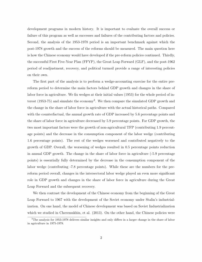
Figure 1 shows aggregate and sectoral, agricultural and non-agricultural, data for China for

1952-2012. We divide the discussion of this period into two subperiods: pre- and post- 1978

reforms.

China 1952-1978

The Chinese economy in 1952-1978 grew rather rapidly, with a 3.6 percent average rate of

growth of real GDP per capita. However, the economy did not experience structural transfor-

mation. In 1952, the primary occupation for 83 percent of the working-age Chinese population

was agriculture. This fraction declined very slowly (with the exception of the brief period dur-

ing the GLF when about 20 percent of the labor force temporarily moved from agriculture to

manufacturing), remaining above 80 percent until 1970 and declining to 75 percent in 1977.

The role of agriculture in GDP was also very important, with more than 70 percent of value

added produced in agriculture in 1952, declining only to 30 percent in 1977 (with a similarly

brief downward shift during the GLF). International trade was rather insignificant – China’s

net export of agricultural production was only 3 percent prior to the GLF and declined to

zero after 1960. The imports of non-agricultural goods constituted an even smaller fraction of

non-agricultural value added in the same period. Defense spending was a large component of

manufacturing production accounting for 6 percent of GDP.

China 1978-2012

In 1978-2012 annual growth in real GDP per capita increased to 8.4 percent annually. This

coincides with a rapid increase in investments (as a share of GDP) and reallocation of labor

from agriculture to non-agriculture. The share of labor force in agriculture fell from 75 percent

in 1977 to 33 percent in 2012. The share of value added produced in the agricultural sector

fell from 30 percent to 5 percent respectively. Defense expenditures declined from 6 percent of

GDP to 1.5 percent of GDP in the late 1980s. The relative prices of non-agricultural goods

show a 40 percent appreciation in the 5 years following the reforms, and then continued to

appreciate. Non-agricultural value added shows remarkable growth throughout both periods,

growing at 10.5 and 10.1 percent, respectively. Agricultural value added grew much slower, at

2.0 percent prior to reforms, and 4.4 percent afterwards. The ratios of sectoral capital stock to

sectoral GDP remain roughly stable over the whole period.

11

Annual Growth Ratepre-1978 post-GLF (1966-1975) post-1978

Real GDP 6.0 5.7 9.4Agricultural value added 2.0 2.0 4.5Non-agricultural value added 10.5 7.8 10.2Labor Force 2.5 2.5 1.5Share of Labor Force in Agriculture -0.7 -1.2 -2.2Capital Stock 11.0 7.9 10.2

Table 1: Changes in economic indicators pre- and post-1978.

4 Measurement of wedges in the data

In this section we discuss the choice of parameters that we use to measure sectoral productivities,

wedges (8), (9) and (10), and their components.

4.1 Parametrization

For our baseline preference specification we chose a commonly used Stone-Geary specification

which sets σ = 1. Parameter η measures the long run share of agricultural consumption and

we set it to 0.15. These parameters are consistent with the literature that used the two sector

growth model to study growth and structural transformation in a variety of historical episodes6.

We set the subsistence level to 54 yuan per capita per year in 1978 prices. This subsistence

level accounts for 53 percent of agricultural consumption per capita in 19527. If we set it higher

than 69 percent of consumption of 1952, the simulated economy would go below the subsistence

level in 1960 during the famine of the Great Leap Forward. We explore in an online appendix,

how our main results change in response to alternative calibrations of γA.

We choose the initial capital stock to match the observed level of capital in 1952. Our

technology specification is close to Hayashi and Prescott (2008). The elasticities for the agri-

cultural sector are also in line with estimates of Tang (1984), who uses the contributions of

labor, capital and land at 0.5, 0.1 and 0.25 respectively, with the remaining share of 0.15 as-

signed to intermediate inputs.8 However, there is a large variation in estimates of factor shares6See Caselli and Coleman (2001), Buera and Kaboski (2009, 2012), Herrendorf, Rogerson and Valentinyi

(2013), Stokey (2001). Our parameters are especially close to the calibration in Hayashi and Prescott (2008).The long run share η is also consistent with food expenditure shares in most developed countries.

7The subsistence level is equal to 76 percent of consumption during the famine in 1960.8See p.89 and Appendix Table 9, p.228 in Tang (1984) for the discussion of the consistency of these input

12

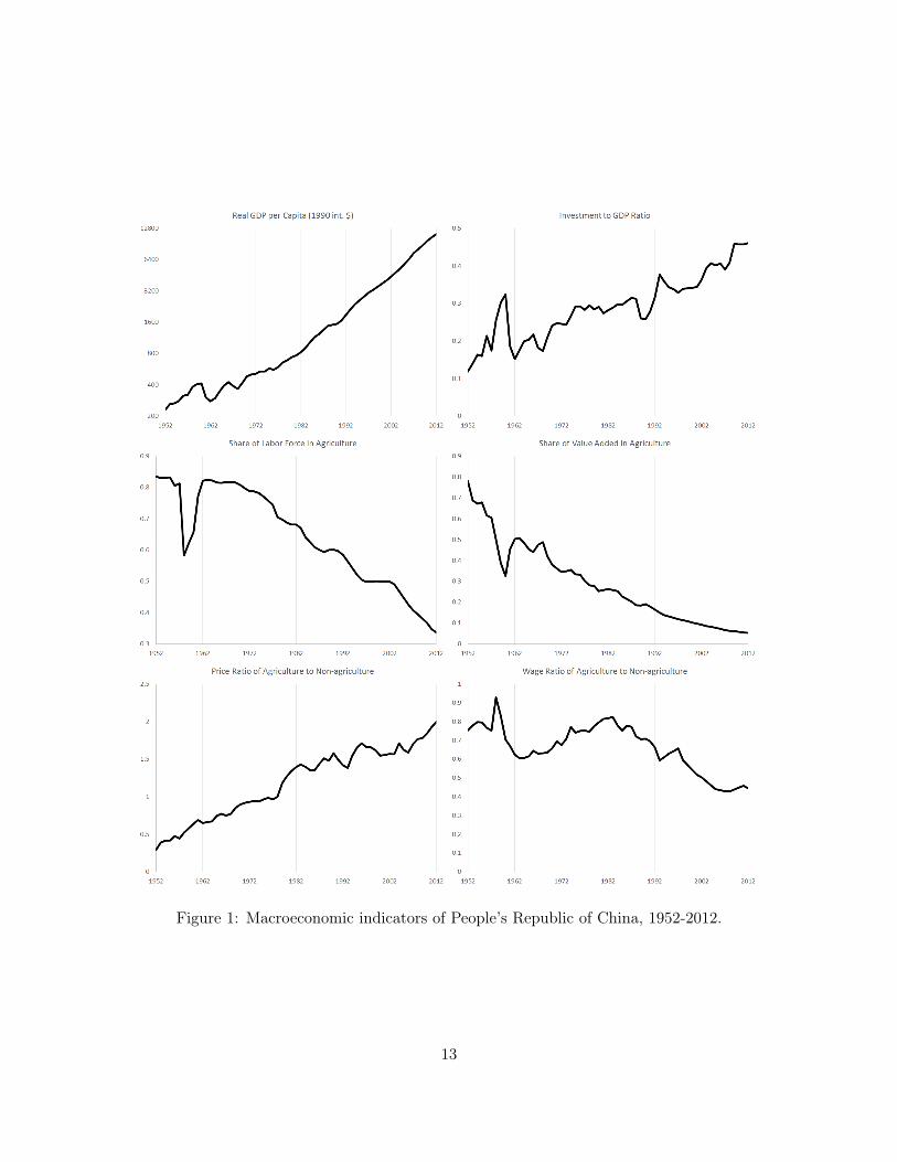
Figure 1: Macroeconomic indicators of People’s Republic of China, 1952-2012.

13

in Chinese agriculture in the literature, neatly summarized by Wen (1993, Table 9, page 27).

Finally, for χt, the path of the fraction of labor force in the population is pinned down by the

data. All our parameters are given in Table 2.

Table 2: ParametersParameter Description ValueαK,A Factor shares 0.14αN,A of the 0.55αK,M production 0.3αN,M functions 0.7γA Subsistence level 54η Asymptotic share 0.15β Discount factor 0.96σ Elasticity of substitution 1.0ρ Intertemporal elasticity 0.0δ Depreciation 0.05

5 Wedge decomposition

We now present the calculation of the total factor productivities XMt , XA

t ; the wedges 1 + τW,t,

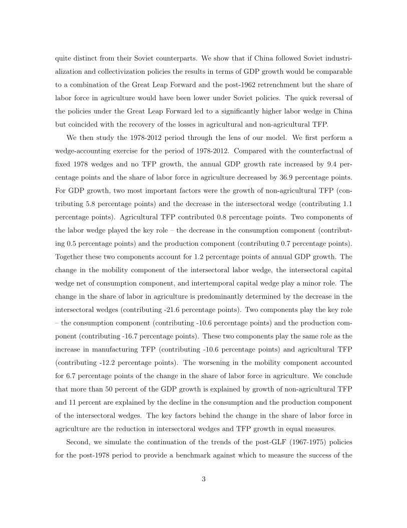
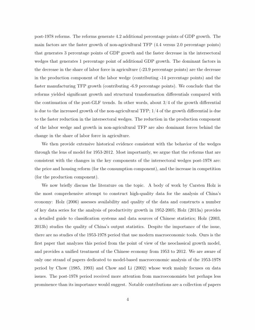
1 + τR,t and 1 + τK,t; and the components of the wedges. Figure 2 plots the agricultural

and non-agricultural TFP and the intersectoral wedges. Figure 3 plots the components of

the wedges.9We report the annual growth rates for the pre-1978 (1952-1978), post Great Leap

Forward period (post-GLF, 1966-1978), and for the post-1978 period in Table 3.10

We now summarize the results of this section. The 1953-1978 period is characterized by

mild growth of TFP (1.9 percent in non-agriculture and 0.3 percent in agriculture), a reduction

in the labor wedge driven by the consumption component, and a reduction in the capital

wedge. The post-GLF period saw an acceleration of agricultural TFP (2.4 percent) and a

deceleration of the reduction in the wedges. After 1978, there was a significant acceleration

of TFP growth, especially in non-agriculture. The reduction in the barriers also significantly

accelerated, especially the production components of the labor wedge.

weights with a number of other countries.9We later show that the investment wedge plays a minor role.

10For the sake of brevity, we refer to the consumption component of the intratemporal labor wedge as “con-sumption”, to the production component of the intratemporal labor wedge as “production”, to the mobilitycomponent of the intratemporal labor wedge as “mobility”, and to the non-consumption component of theintratemporal capital wedge as “capital”.

14

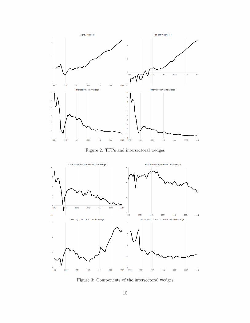
Figure 2: TFPs and intersectoral wedges

Figure 3: Components of the intersectoral wedges

15

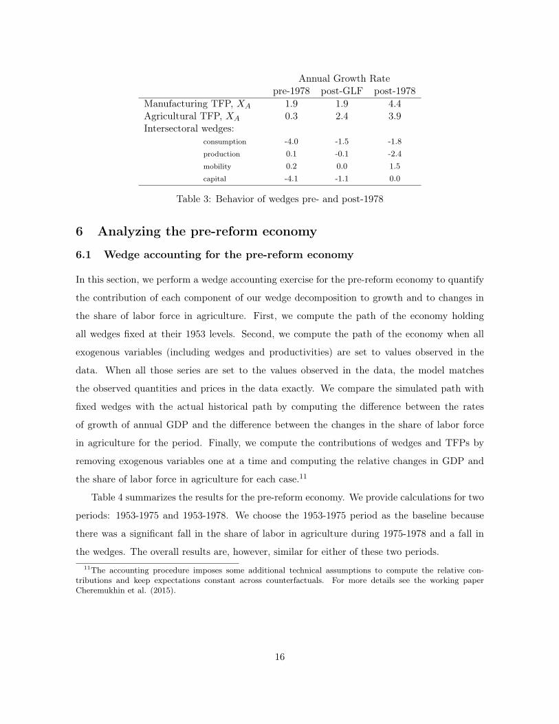
Annual Growth Ratepre-1978 post-GLF post-1978

Manufacturing TFP, XA 1.9 1.9 4.4Agricultural TFP, XA 0.3 2.4 3.9Intersectoral wedges:

consumption -4.0 -1.5 -1.8production 0.1 -0.1 -2.4mobility 0.2 0.0 1.5capital -4.1 -1.1 0.0

Table 3: Behavior of wedges pre- and post-1978

6 Analyzing the pre-reform economy

6.1 Wedge accounting for the pre-reform economy

In this section, we perform a wedge accounting exercise for the pre-reform economy to quantify

the contribution of each component of our wedge decomposition to growth and to changes in

the share of labor force in agriculture. First, we compute the path of the economy holding

all wedges fixed at their 1953 levels. Second, we compute the path of the economy when all

exogenous variables (including wedges and productivities) are set to values observed in the

data. When all those series are set to the values observed in the data, the model matches

the observed quantities and prices in the data exactly. We compare the simulated path with

fixed wedges with the actual historical path by computing the difference between the rates

of growth of annual GDP and the difference between the changes in the share of labor force

in agriculture for the period. Finally, we compute the contributions of wedges and TFPs by

removing exogenous variables one at a time and computing the relative changes in GDP and

the share of labor force in agriculture for each case.11

Table 4 summarizes the results for the pre-reform economy. We provide calculations for two

periods: 1953-1975 and 1953-1978. We choose the 1953-1975 period as the baseline because

there was a significant fall in the share of labor in agriculture during 1975-1978 and a fall in

the wedges. The overall results are, however, similar for either of these two periods.11The accounting procedure imposes some additional technical assumptions to compute the relative con-

tributions and keep expectations constant across counterfactuals. For more details see the working paperCheremukhin et al. (2015).

16

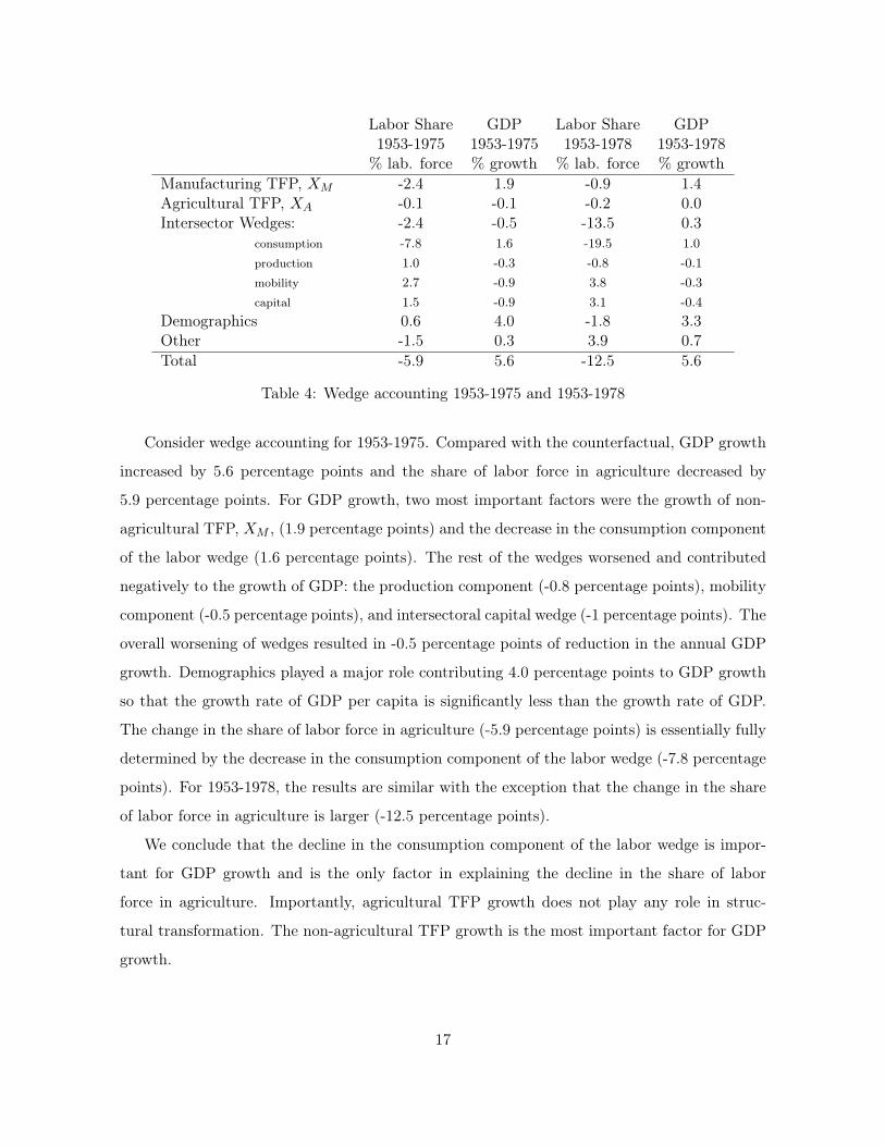
Labor Share GDP Labor Share GDP1953-1975 1953-1975 1953-1978 1953-1978

% lab. force % growth % lab. force % growthManufacturing TFP, XM -2.4 1.9 -0.9 1.4Agricultural TFP, XA -0.1 -0.1 -0.2 0.0Intersector Wedges: -2.4 -0.5 -13.5 0.3

consumption -7.8 1.6 -19.5 1.0production 1.0 -0.3 -0.8 -0.1mobility 2.7 -0.9 3.8 -0.3capital 1.5 -0.9 3.1 -0.4

Demographics 0.6 4.0 -1.8 3.3Other -1.5 0.3 3.9 0.7Total -5.9 5.6 -12.5 5.6

Table 4: Wedge accounting 1953-1975 and 1953-1978

Consider wedge accounting for 1953-1975. Compared with the counterfactual, GDP growth

increased by 5.6 percentage points and the share of labor force in agriculture decreased by

5.9 percentage points. For GDP growth, two most important factors were the growth of non-

agricultural TFP, XM , (1.9 percentage points) and the decrease in the consumption component

of the labor wedge (1.6 percentage points). The rest of the wedges worsened and contributed

negatively to the growth of GDP: the production component (-0.8 percentage points), mobility

component (-0.5 percentage points), and intersectoral capital wedge (-1 percentage points). The

overall worsening of wedges resulted in -0.5 percentage points of reduction in the annual GDP

growth. Demographics played a major role contributing 4.0 percentage points to GDP growth

so that the growth rate of GDP per capita is significantly less than the growth rate of GDP.

The change in the share of labor force in agriculture (-5.9 percentage points) is essentially fully

determined by the decrease in the consumption component of the labor wedge (-7.8 percentage

points). For 1953-1978, the results are similar with the exception that the change in the share

of labor force in agriculture is larger (-12.5 percentage points).

We conclude that the decline in the consumption component of the labor wedge is impor-

tant for GDP growth and is the only factor in explaining the decline in the share of labor

force in agriculture. Importantly, agricultural TFP growth does not play any role in struc-

tural transformation. The non-agricultural TFP growth is the most important factor for GDP

growth.

17

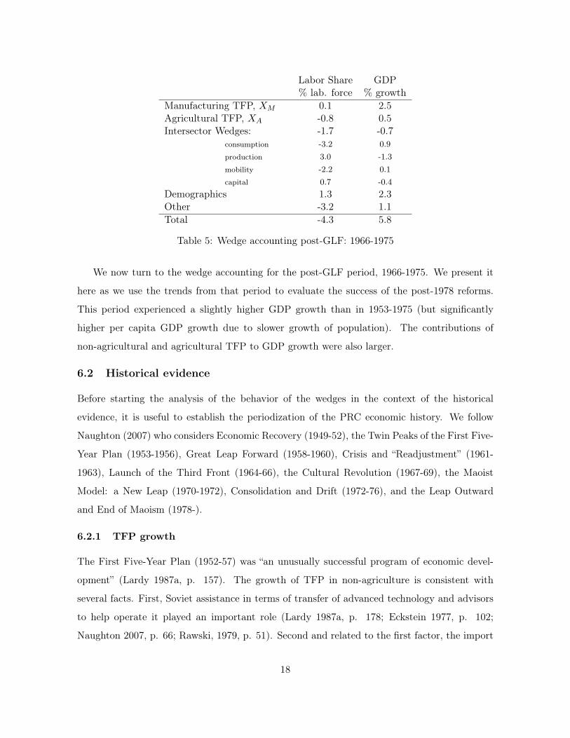
Labor Share GDP% lab. force % growth

Manufacturing TFP, XM 0.1 2.5Agricultural TFP, XA -0.8 0.5Intersector Wedges: -1.7 -0.7

consumption -3.2 0.9production 3.0 -1.3mobility -2.2 0.1capital 0.7 -0.4

Demographics 1.3 2.3Other -3.2 1.1Total -4.3 5.8

Table 5: Wedge accounting post-GLF: 1966-1975

We now turn to the wedge accounting for the post-GLF period, 1966-1975. We present it

here as we use the trends from that period to evaluate the success of the post-1978 reforms.

This period experienced a slightly higher GDP growth than in 1953-1975 (but significantly

higher per capita GDP growth due to slower growth of population). The contributions of

non-agricultural and agricultural TFP to GDP growth were also larger.

6.2 Historical evidence

Before starting the analysis of the behavior of the wedges in the context of the historical

evidence, it is useful to establish the periodization of the PRC economic history. We follow

Naughton (2007) who considers Economic Recovery (1949-52), the Twin Peaks of the First Five-

Year Plan (1953-1956), Great Leap Forward (1958-1960), Crisis and “Readjustment” (1961-

1963), Launch of the Third Front (1964-66), the Cultural Revolution (1967-69), the Maoist

Model: a New Leap (1970-1972), Consolidation and Drift (1972-76), and the Leap Outward

and End of Maoism (1978-).

6.2.1 TFP growth

The First Five-Year Plan (1952-57) was “an unusually successful program of economic devel-

opment” (Lardy 1987a, p. 157). The growth of TFP in non-agriculture is consistent with

several facts. First, Soviet assistance in terms of transfer of advanced technology and advisors

to help operate it played an important role (Lardy 1987a, p. 178; Eckstein 1977, p. 102;

Naughton 2007, p. 66; Rawski, 1979, p. 51). Second and related to the first factor, the import

18

of the capital intensive goods and machinery (also to a large extent from USSR) played an

important role in allowing the economy to operate the “frontier technology” (Naughton 2007,

p.66). Third, the First Five-Year plan model was a technocratic approach with a management

model that placed responsibilities on a director of enterprises, utilized technical experts, and

stressed individual incentives (Eckstein 1977, p. 89-90; Selden 1979, p. 153).12 The growth

of TFP in agriculture during 1952-1957 is consistent with several facts. First, the process of

collectivization in China “limited the disorder and destruction of economic resources” (Teiwes

1987, p.111). Second, more efficient methods of agricultural production were implemented.

Nolan (1976) gives detailed figures and determines five such methods: (1) increase in irrigated

areas; (2) increased multiple cropping; (3) afforestation; (4) improved seeds; (5) increased col-

lection and application of organic fertilizers (see also Naughton 2007, Chapter 11). Thirdly, the

collectivization led to consolidation in the land plots that led to improvement in agricultural

productivity (Spence 2013, p. 491).

During the Great Leap Forward (1958-1962), TFP in agriculture fell by 41 percent from

its peak in 1958 to the trough in 1962; TFP in manufacturing fell in 1958 by 23 percent and

again in 1961 by 26 percent. One important factor that affected TFP in both agriculture and

non-agriculture was worsening of incentives (Naughton 2007, p. 69; Lardy 1987b, p. 365) as

monetary rewards were prohibited, free markets in the countryside were curtailed, and restric-

tions on the productive private farming plots were placed. The fall in manufacturing TFP

is consistent with several factors. First, the collapse of agricultural production led to severe

shortage of agricultural materials for textile and food-processing industries. Second, many

small scale plants such as backyard steel furnaces were exceptionally inefficient (e.g., Eckstein,

1977, p. 124).13 Third, the Sino-Soviet split led to the departure of virtually all Soviet advisors

in the late summer and early fall of 1960. This meant that a large number of capital-goods

projects had to be suspended (Eckstein, 1977, p.203; Selden 1979, p. 97). The reversal of

the manufacturing TFP fall after 1961 is consistent with the general “readjustment and con-

solidation” policies that refocused industrial production to more specific and high productivity12Another factor that affected TFP in both the agricultural and the non-agricultural sectors of the economy

is the advances in basic hygiene, disease, and pest control that affected productivity and longevity (see, e.g.Spence 2013, p. 488).

13Selden (1979, p. 100) gives the following estimates for these furnaces. In July 1958, there were 30-50thousand small furnaces, in October – close to 1 million. By October 1960, only over 3000 were still operational,and the rest shut down. He further quotes an editorial from People’s Daily of August 1, 1959: “We must facethe problem frankly: Last year’s small furnaces could not produce iron”.

19

projects (e.g., petrochemical and fertilizer), and to a revival of material incentives (Eckstein,

1977 p. 126). The fall in TFP in agriculture is consistent with several factors. One factor was

that productivity fell due to poor management of agriculture under the commune system.14 Li

and Yang (2005)15 argue that the most important causal factors in the collapse of agricultural

output between 1958 and 1961 were, in order of importance: (1) the diversion of resources from

agriculture; (2) excessive procurement of grain affecting physical strength of the peasantry; (3)

bad weather. The fall in productivity was reversed only after 1962.

The period of 1962-1966 was a period of recovery from the disaster of the Great Leap

Forward. “Agriculture first” strategy included reopening of private plots (Lardy 1987b, p. 389),

decentralization of commune management that essentially decreased the size of the production

unit to that in 1955-56, and greater reliance on material incentives (Eckstein, 1977 p. 60-

61). Mao recognized that “backyard furnaces” were a mistake16. Agricultural TFP grew by 35

percent from the low of 1962 to the peak of 1966, but was still 25 percent below the peak of

1958. The increase in agricultural TFP is consistent with the continuation of the “readjustment

and recovery” policy in agriculture. Manufacturing TFP grew quickly — recovered to the pre-

crisis peak of 1957 in 1964, and increased by almost 60 percent from the low of 1961 to the

peak of 1966.

The next subperiod (1967-69) is that of the peak of the Cultural Revolution.17 Despite the

exceptional importance of the events of the Cultural Revolution for the country, the economic

implications were much more muted. The fall in agricultural and manufacturing TFP in 1967

and 1968 was relatively minor, and agriculture was affected less than manufacturing. Sectoral

TFPs reached or exceeded the peak of 1966 already in 1970. This is consistent with the

conclusion of Perkins (1991, p. 482-483) that “In short, all of the worker strikes, the battles

between workers and Red Guards, and the use of the railroads to transport Red Guards around14Lin (1990) discusses a variety of hypotheses and presents a view emphasizing the role of incentives in the

fall of productivity. See also Donnithorne (1987, Chapter 2) for the detailed description of the evolution of thecommunes. Considering the negative productivity impact of the communes Lardy (1987b, p. 370) argues thatthe most important factor was in the poor construction and design of the irrigation projects which reducedrather than raised yields (See also Cheng 1982, p. 267).

15See also an extensive discussion in Bramall (2009, p.128-134) of the literature on the causal factors of thecollapse of agricultural production and the famine.

16Mao Tse-tung, “Speech at the Lushan Conference,” 23 July 1959, in Stuart Schram, ed. “Chairman Maotalks to the people,” 142-43, cited by Perkins, 1991, p. 478

17Historians typically define the period of Cultural Revolution starting in late 1965 and ending with theconvocation of the Ninth National Congress of the Chinese Communist Party in April 1969 (e.g., Harding 1991,p. 111) .

20

the country had cost China two years of reduced output but little more, at least in the short

run... the contrast between the disruption caused by the Cultural Revolution and that resulting

from the Great Leap Forward of 1958-60 is striking” and that “The Cultural Revolution at its

peak (1967-68) was a severe but essentially temporary interruption of a magnitude experienced

by most countries at one time or another.” (Perkins 1991, p. 486). Naughton (2007, p. 75)

reaches the same conclusion that “From an economic standpoint, the Cultural Revolution (in

the narrow definition [1966-69]) was, surprisingly, not a particularly important event”.

6.2.2 Wedges

In contrast with several detailed studies of TFP behavior during the pre-reform period described

above there is much less literature on the potential wedges. That is why, rather than focusing on

the detailed exposition that we have done for TFP, we view this section as describing evidence

that is broadly consistent with the patterns of the wedges.

Consumption component of the intersectoral wedges The consumption component of

the wedge starts from the very high level in 1952-1953 and is driven by the very low level of

consumption of non-agricultural goods. The reason is as follows. We calculate non-agricultural

consumption as the residual of non-agricultural output after investment. Since we assume in

the model that all investment is done in non-agricultural goods, the level of this component and

the overall wedge for those years is very sensitive to the data on investment. Almost certainly,

we overestimate the level of this component of the wedge for these years. At the same time, as

we discussed in the previous section this was the period of the First Five Year Plan that placed

heavy emphasis on investment and this is consistent with the high level of the consumption

wedge.

During the Great Leap Forward, the dominant factor driving the consumption wedge was

the catastrophic collapse of agricultural consumption that moved aggregate consumption very

close to the subsistence level. This approaching of the subsistence level of consumption and

the shortages of agricultural goods are both consistent with the consumption component of the

intrasectoral wedges falling significantly.

A useful proxy for the degree of intervention in the agricultural markets is the level of state

procurement. Depending on how exactly procurement is modeled, it can represent itself in

21

various wedges – either in consumption or in the production component of the wedge, or as

we argued in the previous section – in the TFP wedge. The changes in the agricultural policy

during the Great Leap Forward were so large and abrupt that most likely procurement affected

a variety of wedges. Since the TFPs and wedges behaved similarly – experiencing a rapid fall

and then a rapid recovery – we use procurement to provide indirect evidence for the behavior

of these wedges.

The level of state procurement of grain reached its peak in 1959 and rural retentions per

capita reached the trough in 1960 (Lardy 1987b, p. 381 Table 7; Li and Yang 2005, Table

1). The combination of high plans (and therefore procurement quota) and low output resulted

in severe shortage of agricultural goods and a great famine which cost about 30 million lives

(Meng et al., 2013). For example, retained grain per person fell from 273 kilograms per capita

in 1957 to 193 kilograms in 1959, and to 182 kilograms in 1960 (Li and Yang 2005, Table

1); or from 227 kilograms in 1959, to 215 kilograms in 1960, and to 207 kilograms in 1961 if

one accounts for re-sales (Ash 2006, Table 5). Ashton et al. (1984, Table 5) estimate that

average daily calorie consumption was a shocking 1534 Kcal in 1960. Lardy (1983, p.150)

documents severe shortages of food in 1961 and 1962. Lardy (1987b, p. 375) cites the evidence

of the shortage represented in the “extraordinary increase in rural [unregulated] market prices of

available foodstuff”. Following the agricultural crisis, first attempts to scale back procurement

were evidenced in 1961. Also, in the winter of 1961, the fixed procurement prices were raised

(Lardy 1987b, p. 385). In 1961-2, procurement was drastically reduced (Li and Yang, 2005,

Table 1; Lardy 1987b, p. 388)18. The average food consumption recovered to 2026 calories in

1964. This decrease in the procurement levels and the eased shortages of the agricultural goods

are consistent with the consumption component of the intersectoral wedge decreasing and then

increasing. Post-1965, grain procurement net of resales stabilized at about 40 percent of output

(Ash, 2006, 1985).

We now discuss a variety of additional evidence that is consistent with the high level of

the consumption component of the wedge and its behavior. A sizable literature studies price

scissors in China (e.g., Yu and Lin 2008). Most of it focuses on the price scissors defined as

the observed terms of trade between the agricultural and the non-agricultural sector. There

are, however, several papers that study the difference between observed prices and prices that18Net of resales procurement as a proportion of grain output started falling in 1960 (Ash 2006, Table 5).

22

would occur if various policies (such as rationing) were removed. Such comparison between the

observed and undistorted prices is similar to our concept of the consumption component of the

wedge. While the models and the periods of study in these papers vary, we view them as a

useful supplement to our analysis supporting our main point that the agricultural prices were

too low, and non-agricultural prices were too high compared with the undistorted benchmark.19

Imai (2000) studies a static, two sector model of the pre-reform (1964-1978) period and finds

that the undistorted agricultural prices would be 35-50 percent higher and the undistorted

purchases of the non-agricultural goods would be on average 59 percent higher (67 percent

higher in 1970-1978). Sheng (1993b) constructs an index of the prices of agricultural goods

on the free markets compared with the state list prices and argues that this ratio ranged from

1.3-1.4 in the 1950s and 1964-1970, and 1.5-1.8 in the first part of the 1970s. During the Great

Leap Forward the ratio increased to 4.12 in 1961 and then decreased to 2.7 in 1962 and 2.2 in

1963. Finally, Table 7 in Zhang and Zhao (2000) summarizes a variety of estimates by Chinese

economists of the degree of unequal exchange between agriculture and manufacturing. These

estimates are based on the Marxist labor theory of value and are not directly comparable with

the analysis here. Still, the broad comparison of the trends is useful. The estimates of unequal

exchange in the 1950s range from 20 to 65 percent. The estimates of the state purchasing

price being below the “real value” for agricultural goods range from 20 percent in the 1950s,

40-80 percent during the Great Leap Forward, and about 50 percent in the 1970s.20 Nolan and

White (1984) summarize: “Chinese economists now are generally agreed that serious “unequal

exchange” has existed throughout the post-Liberation period (and thus does today) in the

sense that the “price” of industrial commodities is much greater than their “value” (in terms of

embodied labour) and the “price” of agricultural commodities is much below their “value” ”.

Mobility component of the labor wedge We start the discussion of the mobility com-

ponent with its increase in 1955. This is consistent with the start of the implementation of

the hukou system of registration of urban and rural population and the restrictions on their19See also Naughton (2007, p. 60) who argues extensively that such price wedge was a key feature of the

command economic system in China.20We also refer the reader to Cheng (1982, Chapter 7) and Chinn (1980) for an extensive description of

rationing and coupons for both agricultural and non-agricultural goods. While the magnitude and evolution ofthe relative wedge is difficult to assess, Cheng (1982, p. 217) argues that “The most detrimental effect is causedby the separation of production and consumer demand”.

23

movement.21 Nolan and White (2007) argue that the measures to control migration started to

be effective after 1955.

The mobility component decreased by 82 percent from 1957 to 1960 and then increased,

returning to its 1957 level in 1964. It is not surprising that this was accompanied by an un-

precedented increase in the agricultural labor force. The reversal of the barrier is also consistent

with the massive forced resettlement of urban population to the countryside. In 1961-62, about

30 million urbanites were thus moved to the countryside (Lardy 1987b, p. 387).

From 1962 to 1966 the mobility component of the wedge continued its increase which is

consistent with Ministry of Public Security starting to rigorously control and enforce the re-

strictions on rural to urban migration (Chan and Zhang 1999).

Liu (2005) discusses hukou conversion process as a crucial aspect of rural–urban migration

whereas recruitment by state-owned enterprises was the main channel for individuals in rural

areas to obtain an urban hukou during the 1960s and 1970s. The policy of hukou conversion

is consistent with the decline in the mobility component of the wedge, even though it likely

accounts only for part of this decline. Wu (1994) also discusses the policy of sending about

18 million urban youth to villages during Cultural Revolution and their gradual recall back

to the cities. This policy likely had a mixed impact on the mobility wedge – first an increase

and then a decrease. Moreover, in 1971, the government, for the first time since the collapse

of the Great Leap Forward, relaxed control over the increase in permanent positions in the

urban/industrial sector. This policy is consistent with the decrease in the mobility wedge.

Another force affecting the mobility component of the wedge is the return to human capital.

Lower returns to education manifest themselves in the lower non-agricultural wage and a lower

mobility wedge. Fleisher and Wang (2005) provide evidence that returns to schooling measured

as the ratio of the income of college graduates to income of individuals with only elementary

schooling declined from a ratio of 1.8 in the years prior to 1960 to a ratio of about 1.3 in the

years around 1980. They argue that three factors contribute to the decline in the wage gap: (1)

decreased differential between traditionally good (for example, high paying employers owned

by the central government) and bad jobs (Zhou 2000); (2) decreased differential in pay between21While the origins of the hukou system can be traced to 1951, Nolan and White (2007) argue that the

measures to control migration started to be effective after 1955. See Cheng and Selden (1994) for a detailedaccount of the origins of this system and Chan and Zhang (1999) for a comprehensive history of the hukousystem.

24

workers who differ in schooling within jobs; (3) discrimination in the assignment of college

graduates to jobs in favored occupations, industries, and geographical locations, as evidenced,

for example by sending high school graduates to rural jobs (see discussion in Zhou and Hou

1999).

Production component of the labor wedge There is very little data on the size of the

production component of the labor wedge. The only direct evidence we are aware of is the study

by Dong and Putterman (2000) who argue that monopsony in the pre-reform industry was a

significant impediment to structural transformation. They calculate the difference between the

marginal product of labor and wages, including welfare benefits and subsidies, in Chinese state

industry and find that the mean gap was 169 percent and the median gap was 189 percent for

1952-1984.

Intersectoral capital wedge In this section, we discuss the non-consumption component of

the capital wedge in Figure 3, panel 4. The total intersectoral capital wedge is the combination

of the consumption wedge and this component.

In 1952-1957 the intersectoral capital wedge decreased significantly. This is consistent with

the main strategy of the First Five-Year Plan that placed the “overwhelming allocation of

investment resources to industry” and production of capital goods (Lardy 1987a, p.158). Selden

(1979, p. 153) states that the order of economic priorities for that period was: heavy industry,

light industry, agriculture. Lardy (1987a, p. 158) and Eckstein (1977, p. 188) give details

of investment allocation to industry and agriculture to also argue about the low priority of

agricultural investment.

The intersectoral capital wedge decreased significantly to the trough in 1960 and then

started its reversal. This behavior is consistent with several facts. The first years of the

GLF strategy were based on a massive infusion of capital both to the industries developed in

the First-Five Year plan, and importantly to small-scale industrial plants such as “backyard

furnaces” (Lardy 1987b, p. 365)22. The reversal of the wedge afterwards is consistent with

several facts. There was a massive closure of the construction of industrial projects after22While often the first years of the Great Leap Forward are associated with the small scale projects such as

backyard furnaces (see, e.g. discussion in Spence 2013), Lardy (1987b, p. 367) gives detailed statistics on thepreponderance of investment allocation to the medium and large-scale industrial plants.

25

the disastrous first years of the GLF (Lardy 1987b, p. 387) and a corresponding increase in

investment allocated to agriculture. The “Agriculture first” strategy most significantly increased

chemical fertilizer production, electricity allocation, and the production of small agricultural

implements (Eckstein, 1977, p. 60). These measures also are consistent with the increase in

the intersectoral wedge in those years.23 The decline in the non-consumption component of the

capital wedge is consistent with the argument of Perkins (1991, p. 486) who concludes that

the period of 1966-76 was very similar to the original 1950s vision of the First Five-Year Plan.

An additional element was the development of the “Third Front” was a massive construction

program in the inland provinces of the entire industrial base that would not be vulnerable to

the attacks by the Soviets or Americans.24 The Third Front was important even during the

Cultural Revolution, but its rapid expansion phase was stopped by the Cultural Revolution.

Considering the whole period of 1952-1978, the behavior of the capital wedge is consistent

with the classification of the evolution of China’s development strategies by Cheng (1982, Table

9.3) who ranks the sectoral priorities. Only during the Readjustment period of 1961-1965

agriculture received priority consistent with the increasing capital wedge; in all other periods

heavy industry ranked first in the list of priorities consistent with the decline of the capital

wedge.

6.3 Great Leap Forward and Comparison with Soviet Industrialization

In this section, we provide a more detailed analysis of the Great Leap Forward.

We first briefly discuss the simulation of the behavior of the economy assuming that the

Great Leap Forward did not happen25. We linearly extrapolate TFP in both sectors and

the components of the labor and capital wedges between 1957 and 1964 and compute the

counterfactual economy. We find that fluctuations in most of these variables are dampened

in the absence of the GLF. The changes in the intersectoral labor wedge play a dominant

role in explaining the changes in the share of labor force in agriculture during the GLF. The

temporary decrease in the labor wedge accounts for the bulk of the movement of peasants to

the manufacturing sector and then back. However, there is only a temporary positive effect23For example, special allocations of materials to produce small instruments such as hand tools and carts

were implemented in 1962, and the availability of these items was restored to the pre-GLF years (Lardy 1987b,p. 391).

24See Naughton (1988) for a detailed discussion of the industrial policies under the Third Front.25The details of the calculations are in the working paper version Cheremukhin et al. (2015)

26

on GDP, with a slowdown and famine that followed. We note the importance of the changes

in the labor wedge for the behavior of the share of labor force in agriculture and GDP during

that period.

Great Leap Forward was to a large extend modeled on the policies of industrialization

and collectivization in the Soviet Union under Stalin in 1928-1933. In Cheremukhin, et al.

(2013) we found that in the Soviet Union these policies resulted in a significantly reduced labor

wedge and a significant fall in TFP. This parallel with Chinese experience naturally leads to

the comparison with the policies of the Soviet Union under Stalin. We perform the following

counterfactual simulations. We start Stalin’s policies in 1957 (1957 thus being 1928 of Stalin’s

policies). This choice of timing is guided by the idea that the peak of the reforms in China

under the Great Leap Forward (1960) should coincide with the peak of Soviet collectivization

(1932). This is done to isolate GLF, and to study similarities as well as differences between the

GLF and the most intense phase of Stalin’s collectivization.26

Specifically, we use the wedges computed in (Cheremukhin, et al. 2013) for Soviet Russia’s

industrialization and choose the timing of Stalin’s policies to coincide with those of the GLF.

We impose the wedges and sectoral TFPs for Stalin’s 1928-1939 economy on our model of the

Chinese economy over the period 1956-1967. We do this by multiplying each wedge by period-

over-period relative changes in wedges implemented by Stalin. We then compare the actual

data for the Chinese economy to the simulated Chinese economy with Stalin’s policies imposed.

That is, the model in 1957-1968 has the same innovations to wedges and sectoral TFPs as that

of Stalin. After 1968, the economy returns to the same growth rates of wedges and the sectoral

TFPs as in the baseline model.

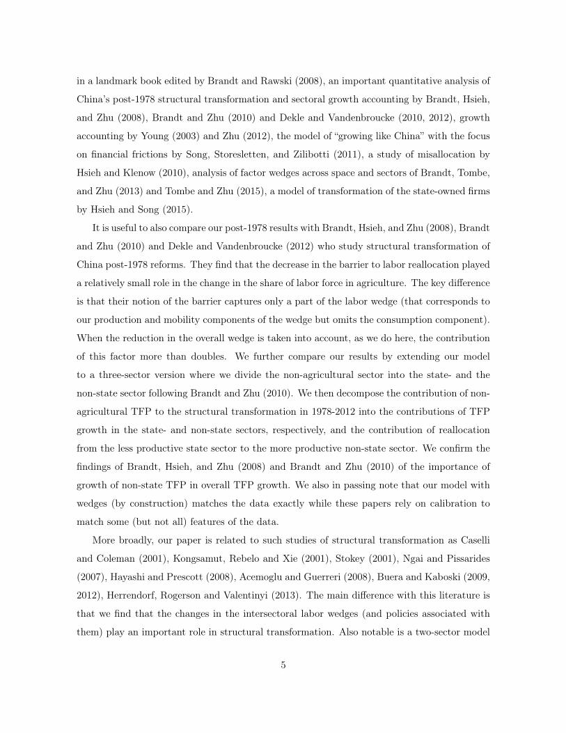
Figure 4 plots both actual Chinese wedges and the simulated economy with Stalin’s wedges.

There are similarities between these economies and some important differences. The main result

of Stalin’s policies would be a much lower share of labor force in agriculture while the behavior

of GDP per capita is broadly the same. We now compare the behavior of the wedges. First, the

fall in agricultural TFP was more significant in China compared with Soviet Russia. The fall in

agricultural TFP from the peak to trough was 20 percent in Soviet Russia versus 41 percent in

China. This is consistent with the more radical way of transforming agriculture in China during

the Great Leap Forward. The rates of recovery post 1962 in China and post 1932 in Soviet26For a survey of the existing literature on exactly this comparison see Yang (2008).

27

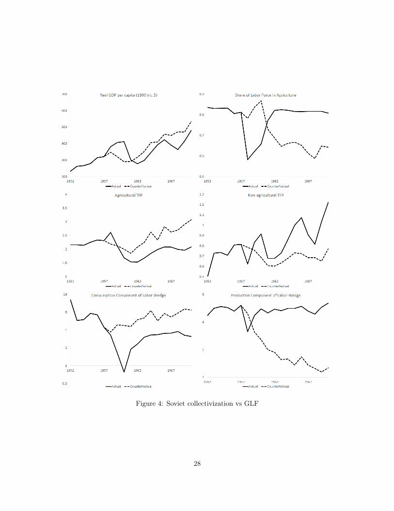
Figure 4: Soviet collectivization vs GLF

28

Russia were rather similar with slightly higher trend growth in China (7.6 percent from 1962 to

1966 in China versus 5.8 percent from 1932 to 1938 in Soviet Russia). Second, non-agricultural

TFP recovered quickly in China and had faster trend growth (1.9 percent from 1960 to 1976

in China versus 1.7 percent from 1933 to 1940 in Soviet Russia). Third, the intersectoral labor

wedge was permanently lowered in Soviet Russia while recovered to pre-GLF levels in China.

The behavior of the components of the wedge was also different. The consumption component of

the wedge in Russia fell less than in China reflecting a less severe fall in agricultural consumption

and being farther away from subsistence. The production component of the intersectoral labor

wedge was permanently lowered in Soviet Russia compared with a decline and then recovery

in China.

We summarize the results as follows. If China followed Soviet industrialization and collec-

tivization policies the results in terms of GDP growth would be comparable to a combination

of the Great Leap Forward and the post-1962 retrenchment but the share of labor would have

been lower under Soviet policies. The quick reversal of the policies under the Great Leap

Forward led to a significantly higher labor wedge in China but coincided with the recovery of

the losses in agricultural and non-agricultural TFP. In contrast, Soviet collectivization would

have achieved a long-term reduction in the labor wedge at a cost of a long-term reduction in

manufacturing TFP. The decline in the intersectoral labor wedge in the counterfactual would

have happened due to two opposing factors. On one hand, there is a significant decrease in the

production component of the wedge, that we emphasized as an important feature of Stalin’s

policies in Cheremukhin et al. (2013). On the other hand, a milder effect of disruption in

consumption of agricultural goods in Soviet Russia resulted in a smaller fall and a higher level

after recovery of the consumption component of the wedge in the counterfactual.

7 Analyzing the economy in 1978-2012

In this section, we first perform a wedge-accounting exercise for the period of 1978-2012, using

the same procedure as in the last section. Second, we simulate the continuation in the post-GLF

(1967-75) trends of the policies in the post-1978 period to provide a benchmark against which

to measure the success of the post-1978 reforms. We then discuss extensive historical evidence

consistent with our findings. Finally, we describe an extension to a three sector model with

private and state firms and provide further decomposition of TFP growth in non-agriculture.

29

7.1 Wedge Accounting 1978-2012

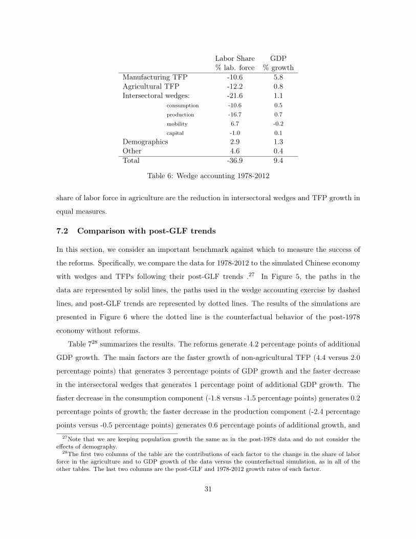
Table 6 summarizes the results. Compared with the counterfactual of fixed 1978 wedges and

no TFP growth, annual GDP growth increased by 9.4 percentage points and the share of labor

force in agriculture decreased by 36.9 percentage points.

For GDP growth (9.4 percentage points per year), two most important factors were the

growth of non-agricultural TFPXM (5.8 percentage points) and the decrease in the intersectoral

wedges (1.1 percentage points). Agricultural TFP contributed 0.8 percentage points. Two

components of the labor wedge played the key role – the decrease in the consumption component

(0.5 percentage points) and the production component (0.7 percentage points) of the wedge.

Together these two components account for 1.2 percentage points of GDP growth. The change

in the mobility component and intersectoral capital wedge play a minor role.

The change in the share of labor force in agriculture (-36.9 percentage points) is predom-

inantly determined by the decrease in the intersectoral wedges (-21.6 percentage points) and

the combined effect of sectoral TFP growth. Two components of the intersectoral wedges play

the key role – the consumption (-10.6 percentage points) and the production (-16.7 percentage

points) components. These two subcomponents play the same role as the increase in manu-

facturing TFP (-10.6 percentage points) and agricultural TFP (-12.2 percentage points). The

worsening in the mobility component accounted for 6.7 percentage points of the change in the

share of labor force in agriculture.

The investment wedge overall plays a minor role for the whole period and we report it as

part of the “Other” category in the table. However, we also performed a finer decomposition

for subperiods and find that the investment wedge was a more important contributor to growth

in the 1990s and 2000s. The average wedge was negative and implied an investment subsidy

on the order of 5 percent. The main effect of the wedge was that it led to an increase in

investment as a share in GDP. Compared with the counterfactual of no subsidy, the investment

wedge accounts for 1.1 percentage points of growth in the 1990s and for 1.5 percentage points

of growth in the 2000s.

We conclude that more than 50 percent of GDP growth is explained by growth in non-

agricultural TFP and 11 percent are explained by the decline in the consumption and the

production components of the intersectoral wedges. The key factors behind the change of the

30

Labor Share GDP% lab. force % growth

Manufacturing TFP -10.6 5.8Agricultural TFP -12.2 0.8Intersectoral wedges: -21.6 1.1

consumption -10.6 0.5production -16.7 0.7mobility 6.7 -0.2capital -1.0 0.1

Demographics 2.9 1.3Other 4.6 0.4Total -36.9 9.4

Table 6: Wedge accounting 1978-2012

share of labor force in agriculture are the reduction in intersectoral wedges and TFP growth in

equal measures.

7.2 Comparison with post-GLF trends

In this section, we consider an important benchmark against which to measure the success of

the reforms. Specifically, we compare the data for 1978-2012 to the simulated Chinese economy

with wedges and TFPs following their post-GLF trends .27 In Figure 5, the paths in the

data are represented by solid lines, the paths used in the wedge accounting exercise by dashed

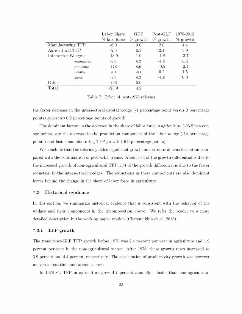
lines, and post-GLF trends are represented by dotted lines. The results of the simulations are

presented in Figure 6 where the dotted line is the counterfactual behavior of the post-1978

economy without reforms.

Table 728 summarizes the results. The reforms generate 4.2 percentage points of additional

GDP growth. The main factors are the faster growth of non-agricultural TFP (4.4 versus 2.0

percentage points) that generates 3 percentage points of GDP growth and the faster decrease

in the intersectoral wedges that generates 1 percentage point of additional GDP growth. The

faster decrease in the consumption component (-1.8 versus -1.5 percentage points) generates 0.2

percentage points of growth; the faster decrease in the production component (-2.4 percentage

points versus -0.5 percentage points) generates 0.6 percentage points of additional growth, and27Note that we are keeping population growth the same as in the post-1978 data and do not consider the

effects of demography.28The first two columns of the table are the contributions of each factor to the change in the share of labor

force in the agriculture and to GDP growth of the data versus the counterfactual simulation, as in all of theother tables. The last two columns are the post-GLF and 1978-2012 growth rates of each factor.

31

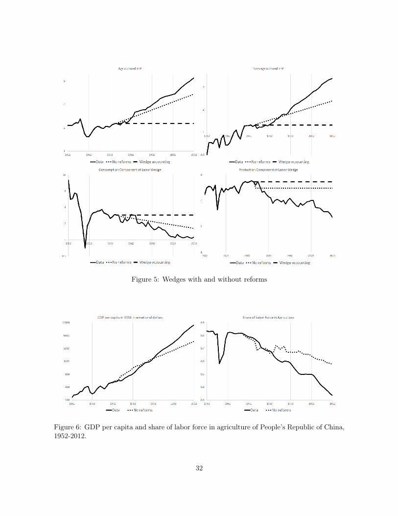
Figure 5: Wedges with and without reforms

Figure 6: GDP per capita and share of labor force in agriculture of People’s Republic of China,1952-2012.

32

Labor Share GDP Post-GLF 1978-2012% lab. force % growth % growth % growth

Manufacturing TFP -6.9 3.0 2.0 4.4Agricultural TFP -2.5 0.3 2.4 3.9Intersector Wedges: -13.9 1.0 -1.8 -3.7

consumption -3.0 0.2 -1.5 -1.8production -12.9 0.6 -0.5 -2.4mobility 4.0 -0.1 0.2 1.5capital -2.0 0.2 -1.0 0.0

Other -0.6 0.0Total -23.9 4.2

Table 7: Effect of post-1978 reforms

the faster decrease in the intersectoral capital wedge (-1 percentage point versus 0 percentage

points) generates 0.2 percentage points of growth.

The dominant factors in the decrease in the share of labor force in agriculture (-23.9 percent-

age points) are the decrease in the production component of the labor wedge (-14 percentage

points) and faster manufacturing TFP growth (-6.9 percentage points).

We conclude that the reforms yielded significant growth and structural transformation com-

pared with the continuation of post-GLF trends. About 3/4 of the growth differential is due to

the increased growth of non-agricultural TFP; 1/4 of the growth differential is due to the faster

reduction in the intersectoral wedges. The reductions in these components are also dominant

forces behind the change in the share of labor force in agriculture.

7.3 Historical evidence

In this section, we summarize historical evidence that is consistent with the behavior of the

wedges and their components in the decomposition above. We refer the reader to a more

detailed description in the working paper version (Cheremukhin et al. 2015).

7.3.1 TFP growth

The trend post-GLF TFP growth before 1978 was 2.4 percent per year in agriculture and 1.9

percent per year in the non-agricultural sector. After 1978, these growth rates increased to

3.9 percent and 4.4 percent, respectively. The acceleration of productivity growth was however

uneven across time and across sectors.

In 1978-85, TFP in agriculture grew 4.7 percent annually - faster than non-agricultural

33

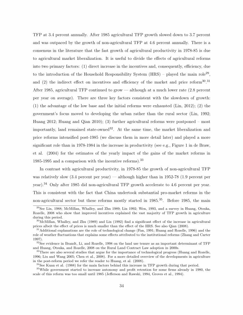
TFP at 3.4 percent annually. After 1985 agricultural TFP growth slowed down to 3.7 percent

and was outpaced by the growth of non-agricultural TFP at 4.6 percent annually. There is a

consensus in the literature that the fast growth of agricultural productivity in 1978-85 is due

to agricultural market liberalization. It is useful to divide the effects of agricultural reforms

into two primary factors: (1) direct increase in the incentives and, consequently, efficiency, due

to the introduction of the Household Responsibility System (HRS) – played the main role29,

and (2) the indirect effect on incentives and efficiency of the market and price reform30.31

After 1985, agricultural TFP continued to grow — although at a much lower rate (2.8 percent

per year on average). There are three key factors consistent with the slowdown of growth:

(1) the advantage of the low base and the initial reforms were exhausted (Lin, 2012); (2) the

government’s focus moved to developing the urban rather than the rural sector (Lin, 1992;

Huang 2012; Huang and Qian 2010); (3) further agricultural reforms were postponed – most

importantly, land remained state-owned32. At the same time, the market liberalization and

price reforms intensified post-1985 (we discuss them in more detail later) and played a more

significant role than in 1978-1984 in the increase in productivity (see e.g., Figure 1 in de Braw,

et al. (2004) for the estimates of the yearly impact of the gains of the market reforms in

1985-1995 and a comparison with the incentive reforms).33

In contrast with agricultural productivity, in 1978-85 the growth of non-agricultural TFP

was relatively slow (3.4 percent per year) — although higher than in 1952-78 (1.9 percent per

year).34 Only after 1985 did non-agricultural TFP growth accelerate to 4.6 percent per year.

This is consistent with the fact that China undertook substantial pro-market reforms in the

non-agricultural sector but these reforms mostly started in 1985.35. Before 1985, the main29See Lin, 1988; McMillan, Whalley, and Zhu 1989; Lin 1992; Wen, 1993, and a survey in Huang, Otsuka,

Rozelle, 2008 who show that improved incentives explained the vast majority of TFP growth in agricultureduring this period.

30McMillan, Whalley, and Zhu (1989) and Lin (1992) find a significant effect of the increase in agriculturalprices albeit the effect of prices is much smaller than the effect of the HRS. See also Qian (2008).

31Additional explanations are the role of technological change (Fan, 1991; Huang and Rozelle, 1996) and therole of weather fluctuations that explains some effects attributed to the institutional reforms (Zhang and Carter1997).

32See evidence in Brandt, Li, and Rozelle, 1998 on the land use tenure as an important determinant of TFPand Huang, Otsuka, and Rozelle, 2008 on the Rural Land Contract Law adoption in 2000s.

33There are also several studies that argue for the importance of technological progress (Huang and Rozelle,1996; Liu and Wang 2005; Chen et al., 2008). For a more detailed overview of the developments in agriculturein the post-reform period we refer the reader to Huang, et al. (2008).

34See Kuan et al. (1988) for the main factors behind this increase in TFP growth during that period.35While government started to increase autonomy and profit retention for some firms already in 1980, the

scale of this reform was too small until 1985 (Jefferson and Rawski, 1994, Groves et al., 1994).

34

effect of the the non-agricultural reforms was in growth of the small rural firms (“township

and village enterprises”, or TVEs)36. But the most important changes in the non-agricultural

sector came after 1984; this is consistent with the rapid acceleration of non-agricultural TFP

growth in 1985-2012 (4.6 percent per year on average). Building on the success of the household

responsibility system in agriculture, the government introduced a dual-pricing system and a

contract management responsibility system (CMRS) in state-owned industrial enterprises (Wu

and Zhao, 1987; Groves et al., 1994; Chen, 1995, Lau et al., 2000). The contract management

responsibility system (CMRS) provided the state-owned industrial enterprises with autonomy

to retain profits and flexibility to set wages and bonuses and had a significant positive effect on

productivity (Groves et al., 1994). Overall, Li (1997) shows that over 87 percent of industrial

TFP growth in the 1980s was attributable to improved incentives, intensified product market

competition, and improved factor allocation37.

7.3.2 Consumption component of the intersectoral labor wedge

The first important policy that is consistent with the behavior of the consumption component

of the labor wedge is the reform of the price and distribution system. The economy experienced

a gradual shift from the system in which a large number of prices were planned, agricultural

and non-agricultural goods were rationed, and the severe shortages were the norm. In 1978-

1983, the prices received by farmers were rapidly increased by a series of decrees but the state

distribution system remained largely in place. By 1984, Whyte (1996, p. 61) argues that the

most significant shortages of key agricultural goods had been substantially decreased. At the

same time, significant shortages of non-agricultural goods remained, especially of energy and

raw materials (Naughton 1996, p. 222). The increase in agricultural prices and the reduction

in rationing, and the decrease in shortages of food are consistent with the increase in the wedge

during that period. The speed of liberalization significantly increased in 1984 with an effort to36See an extensive discussion of the TVEs and the causes of their growth in Naughton (1996, p. 144-169).37There is a significant body of work studying productivity growth in Chinese industry. Brandt, Rawski, and

Sutton (2008) is a comprehensive study of China’s industrial development. Jefferson and Rawski (1994, Table4) and Jefferson, et al. (2000) provides a detailed comparison of the state and the collective-sector productivity.Dougherty et al. (2007) contrasts private and public firms. Chen, et al. (2011, Table 1) summarize variousestimates of the productivity growth noting that there is large variability in them. Brandt et al. (2012) presenta comprehensive set of firm-level productivity estimates for Chinese manufacturing that spans China’s entryinto the World Trade Organization (WTO) and argue that about two-thirds of productivity growth can becontributed to net entry and the growth of entrants. Finally, Tian and Yu (2012) provide a metastudy of TFPgrowth in China.

35

decontrol prices of non-staple foods such as poultry and vegetables (Naughton 1996, p. 248).

Importantly, the price reforms also majorly expanded to non-agriculture: in 1984, for 30 types

of products including raw materials in short supply such as copper and zinc (Wiemer and Lu,

1993 p.124); in 1985 for many consumer durables such as sewing machines and watches38; in

1986, for key items with intense excess demand such as famous-brand bicycles in 1986. This

experience is consistent with a significant decline in the consumption component of the wedge.

The concerns over inflation in the late 1980-s brought partial retrenchment of the price reforms

and reimposition of some controls consistent with a brief upward increase in the consump-

tion component of the wedge. In the late 1980s, the main focus was on market liberalization

by reduction in the restrictions on trading of commodities and by commercialization of the

state grain trading system.39 The 1992-1993 period saw a renewal of price reforms with rapid

progress towards market prices, particularly for crucial producer goods such as steel, and full

decontrolling of petroleum prices in 1993 (Naughton 1996, p 289-290). Huang et al. (2007)

summarize: “with the disappearance of the wedges from the marketing and procurement system

[in agriculture], the remaining wedges after the mid-1990s reflect only trade policies and not

trade and domestic policies.” We conclude that by the beginning of the 1990s, the main effects

of the price reform for agricultural and non-agricultural goods and the corresponding reduction

in the consumption component of the wedge had been completed.40

The second important factor consistent with the decline in the consumption component of

the labor wedge is the housing reform. While housing shortage was prevalent since at least the

1950s, it was particularly severe at the end of the Cultural Revolution in 1976.41 The major38Decline in rationing of some non-agricultural goods happened slightly earlier. Derationing of textile and

cloth led to virtual disappearance of coupons for cloth by 1983. During 1982-1983 price controls were eliminatedon more than 500 small consumer goods such as shoelaces and buttons (Naughton 1996, p. 126).

39For a detailed account of price and procurement reforms in 1979-1988 see Sicular (1988a,b).40One important exception was the primary energy sector, especially coal production that supplied 70 percent

of China’s energy needs in 1992. This sector had a very high level of price and quantity control. The reform ofthe sector started only in 1992 and was gradually implemented over the next five years. This likely contributedto the decline of the price wedge even post 1993. The price wedges also remained for some staple foods such asrice and maize and on cotton because of the desire to provide low-cost input for processing sector (Anderson,et al. 2008).

41The average floor space per person then was 3 sq.m. (Wang and Murie 1996; Tables 1-3 in Lee (1988) forthe decline in the residential floor space since 1952). In 1990, the average living space available per person inthe urban areas was only 6.7 square meters, well below the housing norm of 8 sq. m per person. (Chai 1996,p. 274). Wang and Murie (1996) argue that very low rents were the main cause of the shortages and the lowquality of the housing. Wang and Kinsey (1994) argue that strict rationing of housing was prevalent at leastuntil 1987.

36

nationwide housing reform started in 1994.42 The key provisions of the housing reform were

(Table 2 in Wang and Murie 1996): (1) to change the nature of housing from a welfare service

to a consumable commodity; (2) to change the system of distribution from in-kind and free

to monetary and market-based; (3) to change the system of ownership and tenure from public

to private; (4) to move from subsidized minimum rent to market rent. An important recent

paper provides a detailed empirical analysis of the impact of housing reform on consumption

of housing and calculates the degree of misallocation prior to the reform (Wang 2011). The

estimates of mismatch are equal to 15 percent less housing services than the households would

have chosen in the private market. Furthermore, the system of state allocation of housing

reduced welfare of state-owned residents by 25 percent relative to a system in which instead

of subsidized housing the households were able to freely choose market housing. The 1998

decision to further move from in-kind provision of housing by state companies to cash subsidies

allowed to significantly increase house purchases from private developers.43 By the early 2000s,

the housing market was mostly deregulated. This is evidenced for example by the drastic

reduction in housing subsidies. Khan and Riskin (1998, 2005) provide evidence that housing

subsidies reduced from 18 percent to 10 percent of disposable urban income in 1988-95 and from

10 percent to 2 percent in 1995-2002 (in real terms, the per capita housing subsidy declined

in these years by 70 percent).44 Even after 2002, deregulation continued through softening of

the hukou system which is quintessentially a housing ration as it serves as a barrier to a free

housing market.45

We now discuss additional indirect evidence that is also consistent with the decline in the

consumption component of the wedge. First, the project of the World Bank’s Development

Research Group “Estimates of wedges to Agricultural Incentives” (Anderson et al. 2008) finds42For the comprehensive survey of the housing reform see Wang and Murie (1996). Prior to 1994, there were

several experiments with the housing reform but Wang and Murie (1996) conclude that “the current situationis far from that aimed at in the reform plans”. Wang (2011, 2012) and Deng et al. (2014) also argue that themajor reform started in 1994. See also Iyer et al. (2013).

43Deng et al. (2014) argue that it was “the turning point of China’s housing reform”.44It is also important to note that the housing subsidy was much more important than the price subsidy even

in the beginning of the 1990s, further supporting our claim that housing reform was the main reason behindthe reduction in the price wedge in the 1990s. The price subsidy on food and fuel in 1992 was only 4 percent ofthe urban disposable income (Yang and Zhou 1999); net non-housing subsidies declined to 1.25 percent in 1995and to negligible 0.07 percent in 2002 (Khan and Riskin 2005).

45It is interesting to note that the hukou system’s restriction on housing may affect even the high incomemigrants. The governments of more than thirty big cities have implemented a policy of restricted transactionssince 2011 that did not allow purchases of a new house without a local hukou (Song 2014).

37

that the implicit subsidy to agricultural goods was 42.6 percent in the beginning of the 1980s

and reduced virtually to zero by 1995 and that the implicit tax on non-agricultural tradable

goods declined steadily from 43 percent to about 4 percent in the early 2000s. While this

relative terms of trade wedge also reflects the trade frictions and does not directly translate

into the consumption component of the wedge, the behavior of this measure closely tracks the

behavior of the consumption component of the wedge. Secondly, the decline in the consumption

component is consistent with the consumer revolution which started in the 1980s and drastically

expanded the variety of goods and services available (Chai 1996, p. 274). Indeed, consider a

model in which a consumer values a variety of agricultural and non-agricultural goods but the

planner prohibits production of some goods. It is easy to show that an increase in the share of

the newly available non-agricultural goods reduces the consumption component of the wedge

by reducing the relative measure of unproduced goods. The third kind of evidence refers to the

decline in the degree of unequal exchange between agriculture and manufacturing (see Sheng

1993a and Zhang and Zhao, 2000). Yan Ruizhen et al. (Table 5.2 in Sheng 1993a) estimate

that the degree of uneven exchange decreased from 71.9 percent in 1978 to 15.4 in 1987. Niu

et al. (Table 7 in Zhang and Zhao 2000) estimate that the percent by which state purchasing

price is below “real value” for agricultural products decreased from 39 percent in 1981 to 29

percent in 1989.

7.3.3 Production component of the intersectoral labor wedge

Early work of Naughton (1992) argued that relaxation of state monopoly over industry is

“a single simple interpretative framework [that] explains a great deal” about “a range of the

complex changes that Chinese economy is undergoing” and that “The most crucial step in

economic reform was the ending of the government monopoly over the economy, and especially

over industrial production and investment.” (Naughton 1996).

We first focus on studies that measure the markup in industry and its decline which provides

direct evidence corresponding to the decline in the production component of the labor wedge.

An influential paper by Li (1997) studies panel data on 789 state-owned enterprises between

1980 and 1989 and finds that the markup declined by 15 percent. He also concludes that in 1989

monopoly power was still significant. Bai and Qian (2010) compute labor shares of income and

argue that the results of Li (1997) for 1978-1998 were due to the increase in market competition

38

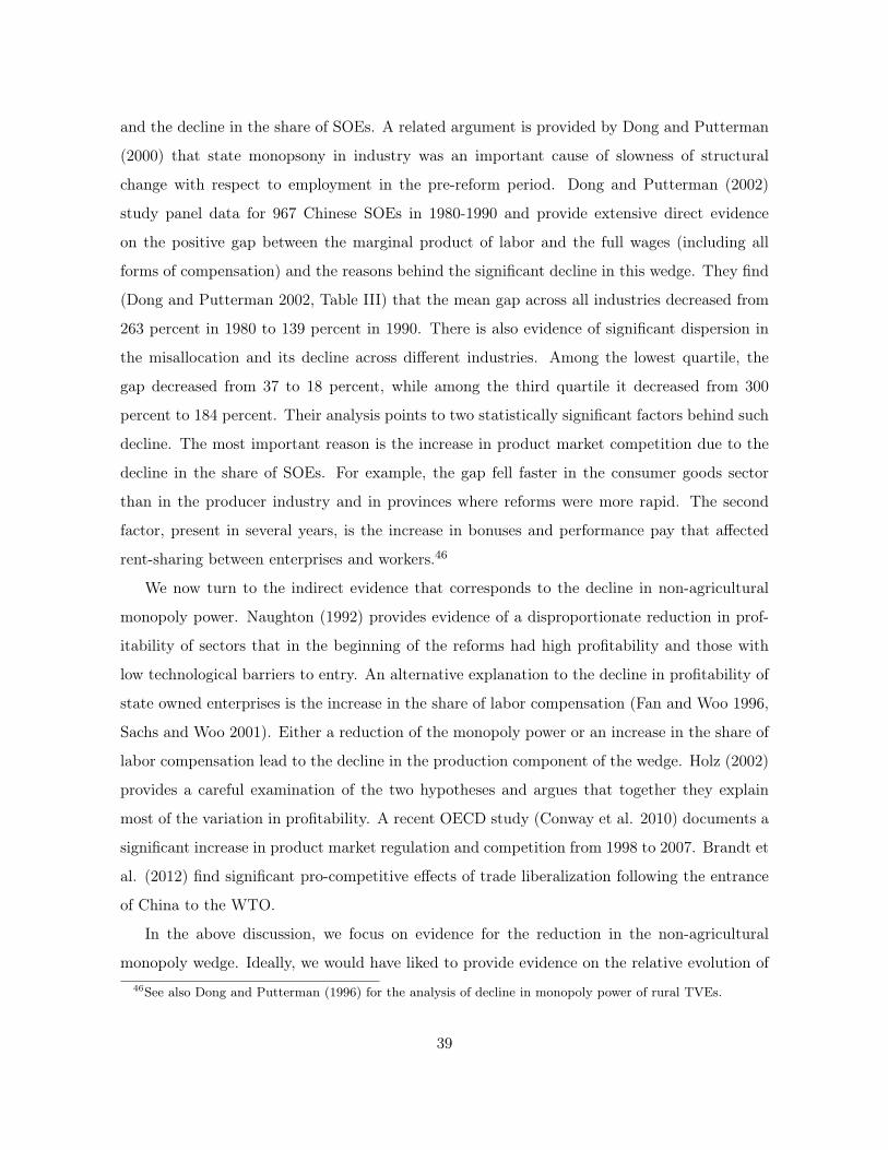
and the decline in the share of SOEs. A related argument is provided by Dong and Putterman

(2000) that state monopsony in industry was an important cause of slowness of structural

change with respect to employment in the pre-reform period. Dong and Putterman (2002)

study panel data for 967 Chinese SOEs in 1980-1990 and provide extensive direct evidence

on the positive gap between the marginal product of labor and the full wages (including all

forms of compensation) and the reasons behind the significant decline in this wedge. They find

(Dong and Putterman 2002, Table III) that the mean gap across all industries decreased from

263 percent in 1980 to 139 percent in 1990. There is also evidence of significant dispersion in

the misallocation and its decline across different industries. Among the lowest quartile, the

gap decreased from 37 to 18 percent, while among the third quartile it decreased from 300

percent to 184 percent. Their analysis points to two statistically significant factors behind such

decline. The most important reason is the increase in product market competition due to the

decline in the share of SOEs. For example, the gap fell faster in the consumer goods sector

than in the producer industry and in provinces where reforms were more rapid. The second

factor, present in several years, is the increase in bonuses and performance pay that affected

rent-sharing between enterprises and workers.46

We now turn to the indirect evidence that corresponds to the decline in non-agricultural

monopoly power. Naughton (1992) provides evidence of a disproportionate reduction in prof-

itability of sectors that in the beginning of the reforms had high profitability and those with

low technological barriers to entry. An alternative explanation to the decline in profitability of

state owned enterprises is the increase in the share of labor compensation (Fan and Woo 1996,

Sachs and Woo 2001). Either a reduction of the monopoly power or an increase in the share of

labor compensation lead to the decline in the production component of the wedge. Holz (2002)

provides a careful examination of the two hypotheses and argues that together they explain

most of the variation in profitability. A recent OECD study (Conway et al. 2010) documents a

significant increase in product market regulation and competition from 1998 to 2007. Brandt et

al. (2012) find significant pro-competitive effects of trade liberalization following the entrance

of China to the WTO.

In the above discussion, we focus on evidence for the reduction in the non-agricultural

monopoly wedge. Ideally, we would have liked to provide evidence on the relative evolution of46See also Dong and Putterman (1996) for the analysis of decline in monopoly power of rural TVEs.

39

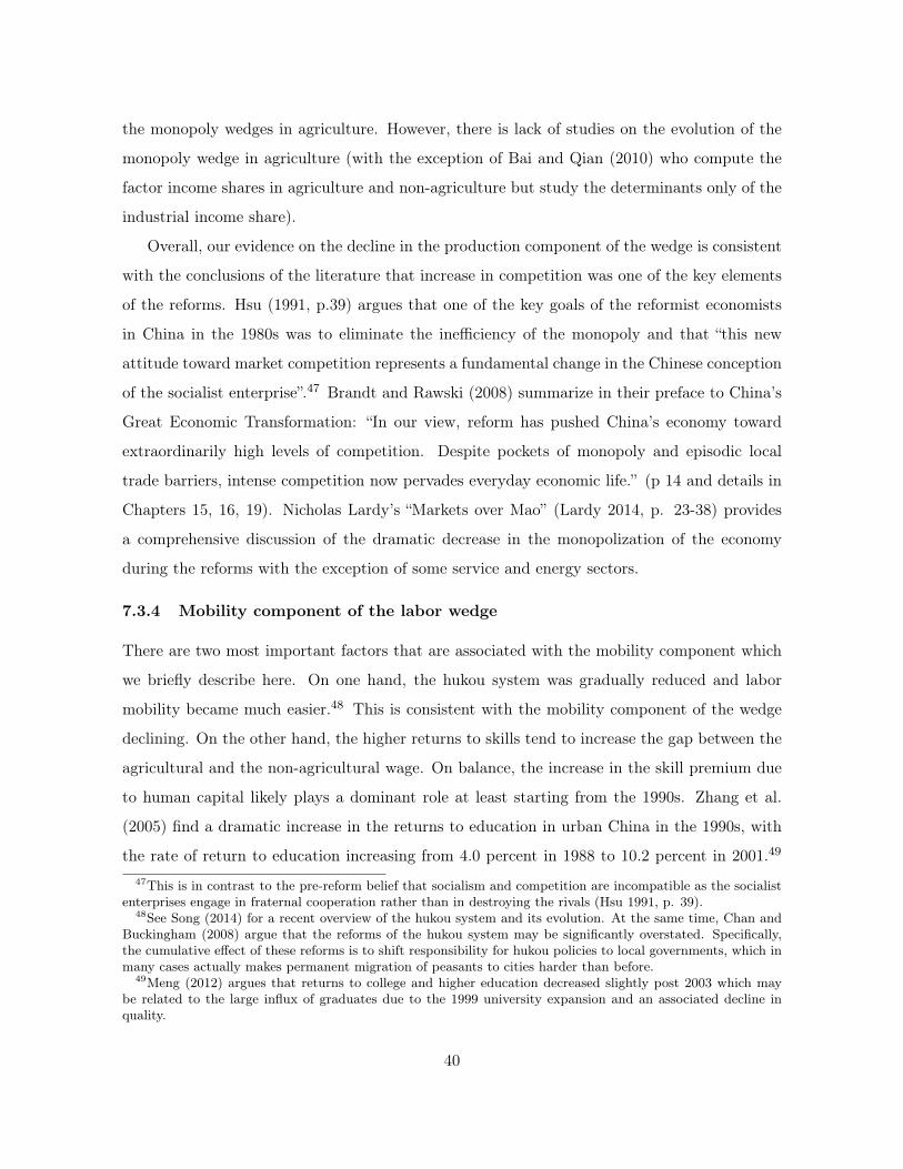
the monopoly wedges in agriculture. However, there is lack of studies on the evolution of the

monopoly wedge in agriculture (with the exception of Bai and Qian (2010) who compute the

factor income shares in agriculture and non-agriculture but study the determinants only of the

industrial income share).

Overall, our evidence on the decline in the production component of the wedge is consistent

with the conclusions of the literature that increase in competition was one of the key elements

of the reforms. Hsu (1991, p.39) argues that one of the key goals of the reformist economists

in China in the 1980s was to eliminate the inefficiency of the monopoly and that “this new

attitude toward market competition represents a fundamental change in the Chinese conception

of the socialist enterprise”.47 Brandt and Rawski (2008) summarize in their preface to China’s

Great Economic Transformation: “In our view, reform has pushed China’s economy toward

extraordinarily high levels of competition. Despite pockets of monopoly and episodic local

trade barriers, intense competition now pervades everyday economic life.” (p 14 and details in

Chapters 15, 16, 19). Nicholas Lardy’s “Markets over Mao” (Lardy 2014, p. 23-38) provides

a comprehensive discussion of the dramatic decrease in the monopolization of the economy

during the reforms with the exception of some service and energy sectors.

7.3.4 Mobility component of the labor wedge

There are two most important factors that are associated with the mobility component which

we briefly describe here. On one hand, the hukou system was gradually reduced and labor

mobility became much easier.48 This is consistent with the mobility component of the wedge

declining. On the other hand, the higher returns to skills tend to increase the gap between the

agricultural and the non-agricultural wage. On balance, the increase in the skill premium due

to human capital likely plays a dominant role at least starting from the 1990s. Zhang et al.

(2005) find a dramatic increase in the returns to education in urban China in the 1990s, with

the rate of return to education increasing from 4.0 percent in 1988 to 10.2 percent in 2001.49

47This is in contrast to the pre-reform belief that socialism and competition are incompatible as the socialistenterprises engage in fraternal cooperation rather than in destroying the rivals (Hsu 1991, p. 39).

48See Song (2014) for a recent overview of the hukou system and its evolution. At the same time, Chan andBuckingham (2008) argue that the reforms of the hukou system may be significantly overstated. Specifically,the cumulative effect of these reforms is to shift responsibility for hukou policies to local governments, which inmany cases actually makes permanent migration of peasants to cities harder than before.

49Meng (2012) argues that returns to college and higher education decreased slightly post 2003 which maybe related to the large influx of graduates due to the 1999 university expansion and an associated decline inquality.

40

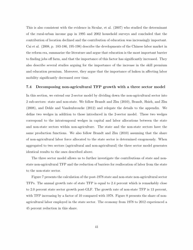
This is also consistent with the evidence in Sicular, et al. (2007) who studied the determinant

of the rural-urban income gap in 1995 and 2002 household surveys and concluded that the

contribution of location declined and the contribution of education was increasingly important.

Cai et al. (2008, p. 183-186, 195-198) describe the developments of the Chinese labor market in

the reform era, summarize the literature and argue that education is the most important barrier

to finding jobs off farm, and that the importance of this factor has significantly increased. They

also describe several studies arguing for the importance of the increase in the skill premium

and education premium. Moreover, they argue that the importance of hukou in affecting labor

mobility significantly decreased over time.

7.4 Decomposing non-agricultural TFP growth with a three sector model

In this section, we extend our 2-sector model by dividing down the non-agricultural sector into

2 sub-sectors: state and non-state. We follow Brandt and Zhu (2010), Brandt, Hsieh, and Zhu

(2008), and Dekle and Vandenbroucke (2012) and relegate the details to the appendix. We

define two wedges in addition to those introduced in the 2-sector model. These two wedges

correspond to the intratemporal wedges in capital and labor allocations between the state

and non-state sectors within non-agriculture. The state and the non-state sectors have the

same production functions. We also follow Brandt and Zhu (2010) assuming that the share

of non-agricultural labor force allocated to the state sector is determined exogenously. When

aggregated to two sectors (agricultural and non-agricultural) the three sector model generates

identical results to the ones described above.

The three sector model allows us to further investigate the contributions of state and non-

state non-agricultural TFP and the reduction of barriers for reallocation of labor from the state

to the non-state sector.

Figure 7 presents the calculation of the post-1978 state and non-state non-agricultural sector

TFPs. The annual growth rate of state TFP is equal to 2.4 percent which is remarkably close

to 2.0 percent state sector growth post-GLF. The growth rate of non-state TFP is 13 percent,

with TFP increasing by a factor of 10 compared with 1978. Figure 8 presents the share of non-

agricultural labor employed in the state sector. The economy from 1978 to 2012 experienced a

45 percent reduction in this share.

41

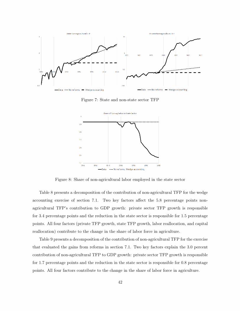
Figure 7: State and non-state sector TFP

Figure 8: Share of non-agricultural labor employed in the state sector

Table 8 presents a decomposition of the contribution of non-agricultural TFP for the wedge

accounting exercise of section 7.1. Two key factors affect the 5.8 percentage points non-

agricultural TFP’s contribution to GDP growth: private sector TFP growth is responsible

for 3.4 percentage points and the reduction in the state sector is responsible for 1.5 percentage

points. All four factors (private TFP growth, state TFP growth, labor reallocation, and capital

reallocation) contribute to the change in the share of labor force in agriculture.

Table 9 presents a decomposition of the contribution of non-agricultural TFP for the exercise

that evaluated the gains from reforms in section 7.1. Two key factors explain the 3.0 percent

contribution of non-agricultural TFP to GDP growth: private sector TFP growth is responsible

for 1.7 percentage points and the reduction in the state sector is responsible for 0.8 percentage

points. All four factors contribute to the change in the share of labor force in agriculture.

42

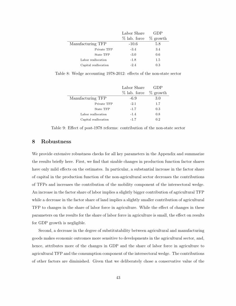
Labor Share GDP% lab. force % growth

Manufacturing TFP -10.6 5.8Private TFP -3.4 3.4State TFP -3.0 0.6

Labor reallocation -1.8 1.5Capital reallocation -2.4 0.3

Table 8: Wedge accounting 1978-2012: effects of the non-state sector

Labor Share GDP% lab. force % growth

Manufacturing TFP -6.9 3.0Private TFP -2.1 1.7State TFP -1.7 0.3

Labor reallocation -1.4 0.8Capital reallocation -1.7 0.2

Table 9: Effect of post-1978 reforms: contribution of the non-state sector

8 Robustness

We provide extensive robustness checks for all key parameters in the Appendix and summarize

the results briefly here. First, we find that sizable changes in production function factor shares

have only mild effects on the estimates. In particular, a substantial increase in the factor share

of capital in the production function of the non-agricultural sector decreases the contributions

of TFPs and increases the contribution of the mobility component of the intersectoral wedge.

An increase in the factor share of labor implies a slightly bigger contribution of agricultural TFP

while a decrease in the factor share of land implies a slightly smaller contribution of agricultural

TFP to changes in the share of labor force in agriculture. While the effect of changes in these

parameters on the results for the share of labor force in agriculture is small, the effect on results

for GDP growth is negligible.

Second, a decrease in the degree of substitutability between agricultural and manufacturing

goods makes economic outcomes more sensitive to developments in the agricultural sector, and,

hence, attributes more of the changes in GDP and the share of labor force in agriculture to

agricultural TFP and the consumption component of the intersectoral wedge. The contributions

of other factors are diminished. Given that we deliberately chose a conservative value of the

43

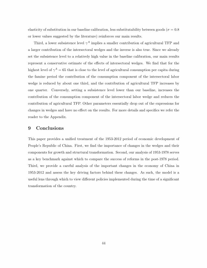
elasticity of substitution in our baseline calibration, less substitutability between goods (σ = 0.8

or lower values suggested by the literature) reinforces our main results.

Third, a lower subsistence level γA implies a smaller contribution of agricultural TFP and

a larger contribution of the intersectoral wedges and the inverse is also true. Since we already

set the subsistence level to a relatively high value in the baseline calibration, our main results

represent a conservative estimate of the effects of intersectoral wedges. We find that for the

highest level of γA = 65 that is close to the level of agricultural consumption per capita during

the famine period the contribution of the consumption component of the intersectoral labor

wedge is reduced by about one third, and the contribution of agricultural TFP increases by

one quarter. Conversely, setting a subsistence level lower than our baseline, increases the

contribution of the consumption component of the intersectoral labor wedge and reduces the

contribution of agricultural TFP. Other parameters essentially drop out of the expressions for

changes in wedges and have no effect on the results. For more details and specifics we refer the

reader to the Appendix.

9 Conclusions

This paper provides a unified treatment of the 1953-2012 period of economic development of

People’s Republic of China. First, we find the importance of changes in the wedges and their

components for growth and structural transformation. Second, our analysis of 1953-1978 serves

as a key benchmark against which to compare the success of reforms in the post-1978 period.

Third, we provide a careful analysis of the important changes in the economy of China in

1953-2012 and assess the key driving factors behind these changes. As such, the model is a

useful lens through which to view different policies implemented during the time of a significant

transformation of the country.

44

10 References

Acemoglu, Daron (2008) Introduction to modern economic growth. Princeton University Press.

Acemoglu, Daron, and Veronica Guerrieri (2008) “Capital Deepening and Non–Balanced

Economic Growth.” Journal of Political Economy, 116, pp. 467–498.

Ahuja, Ashvin (2012) “De-Monopolization Toward Long-Term Prosperity in China.” IMF

Working Paper 12/75.

Anderson, Kym, Marianne Kurzweil, Will Martin, Damiano Sandri, and Ernesto Valenzuela

(2008) “Measuring distortions to agricultural incentives, revisited.” World Trade Review, 7 (4),

pp. 675-704.

Ash, Robert (2006) “Squeezing the peasants: Grain extraction, food consumption and rural

living standards in Mao’s China.” The China Quarterly, 188, pp. 959-998.

Ash, Robert, Christopher Howe, and Y.Y. Kueh (2003) China’s Economic Reform: A Study

with Documents. Routledge Curzon.

Ashton, Basil, Kenneth Hill, Alan Piazza, and Robin Zeitz (1984) “Famine in China, 1958-

61.” Population and Development Review, 10 (4), pp. 613-645.

Bai, Chong-En, and Zhenjie Qian (2010): “The factor income distribution in China: 1978–2007.”

China Economic Review, 21 (4), pp. 650-670.

Bramall, Chris (2009) Chinese economic development. Routledge.

Brandt, Loren, and Thomas G. Rawski, eds. (2008) China’s Great Economic Transforma-

tion. Cambridge University Press.

Brandt, Loren, and Xiaodong Zhu (2010) “Accounting for China’s growth,” IZA Discussion

Paper No. 4764.

Brandt, Loren, Guo Li and Scott Rozelle (1998) “Tenure, land rights, and farmer investment

incentives in China.” Agricultural Economics, 19 (1), pp. 63-71.

Brandt, Loren, Chang-Tai Hsieh, and Xiaodong Zhu (2008) “Growth, and Structural Trans-

formation in China,” in Loren Brandt and Thomas Rawski eds., China’s Great Economic Trans-

formation. Cambridge University Press.

Brandt, Loren, Johannes Van Biesebroeck, and Yifan Zhang (2012) “Creative accounting

or creative destruction? Firm-level productivity growth in Chinese manufacturing.” Journal of

Development Economics, 97 (2), pp. 339-351.

45

Brandt, Loren, Thomas G. Rawski, and John Sutton (2008) “China’s Industrial Develop-

ment,” in Loren Brandt and Thomas Rawski eds., China’s Great Economic Transformation.

Cambridge University Press, pp. 569-632.

Brandt, Loren, Trevor Tombe, and Xioadong Zhu (2013) “Factor Market Distortions across

Time, Space, and Sectors in China.” Review of Economic Dynamics, 16 (1), pp. 39-58.

Brandt, Loren, Johannes Van Biesebroeck, Luhang Wang, and Yifan Zhang (2012) “WTO

Accession and Performance of Chinese Manufacturing Firms.” CEPR Discussion Paper No. 9166.

Buera, Francisco J., and Joe P. Kaboski (2009) “Can traditional theories of structural change

fit the data?” Journal of the European Economic Association, 7 (2-3), pp. 469-477.

Buera, Francisco J., and Joe P. Kaboski (2012) “Scale and the origins of structural change.”,

Journal of Economic Theory, 147 (2), pp. 684-712.

Cai, Fang, Albert Park, and Yaohui Zhao (2008). “The Chinese Labor Market in the Reform

Era,” in Loren Brandt and Thomas Rawski eds., China’s Great Economic Transformation.

Cambridge University Press.

Cao, Shutao and Jing Liu (2011) “Productivity growth and ownership change in China:

1998-2007.” MPRA Paper No. 30571.

Cao, Yuanzheng, Yingyi Qian, and Barry R. Weingast (1999) “From Federalism, Chinese

Style, to Privatization, Chinese Style.” Economics of Transition, 7 (1), pp. 103-131.

Caselli, Francesco, and Wilbur John II. Coleman (2001) “The U.S. structural transformation

and regional convergence: A reinterpretation.” Journal of Political Economy, 109 (3), pp. 584-

616.

Chai, Joseph C.H. (1996) “Consumption and living standard in China”, in Robert Ash and

Y. Y. Kueh eds., Chinese Economy under Deng Xiaoping. Clarendon paperbacks. pp. 247-276.

Chan, Kam Wing and Will Buckingham (2008) “Is China abolishing the hukou system?.”

The China Quarterly, 195, pp. 582-606.

Chan, Kam Wing and Li Zhang (1999). “The Hukou System and Rural-urban Migration:

Processes and Changes.” The China Quarterly, 160 (1), pp. 818-855.

Chari, V. V., Patrick Kehoe, and Ellen McGrattan (2007) “Business cycle accounting.”

Econometrica, 75 (3), pp. 781-836.

Chen, Derong (1995) Chinese Firms Between Hierarchy and Market: The Contract Man-

agement Responsibility System. Macmillan.

46

Chen, Po-Chi, Ming-Miin Yu, Ching-Cheng Chang, and Shih-Hsun Hsu (2008) “Total factor

productivity growth in China’s agricultural sector.” China Economic Review 19 (4), pp. 580-

593.

Chen, Shiyi, Gary H. Jefferson, and Jun Zhang (2011) “Structural change, productivity

growth and industrial transformation in China.” China Economic Review, 22 (1), pp. 133-150.

Cheng, Chu-yuan (1982) China’s Economic Development: Growth and Structural Change.

Westview Press.

Cheng, Tiejun and Mark Selden (1994) “The Origins and Social Consequences of China’s

Hukou System.” The China Quarterly, 139, pp. 644-668.

Cheremukhin, Anton, Mikhail Golosov, Sergei Guriev, and Aleh Tsyvinski (2013) “Was

Stalin Necessary for Russia’s Economic Development?” NBER Working Paper No. 19425.

Cheremukhin, Anton, Mikhail, Golosov, Sergei Guriev, and Aleh Tsyvinski (2015) “The

Economy of People’s Republic of China” NBER Working Paper.

Chinn, Dennis L. (1980) “Basic commodity distribution in the People’s Republic of China.”

The China Quarterly, 84, pp. 744-754.

Choe, Chongwoo and Xiangkang Yin (2000) “Contract management responsibility system

and profit incentives in China’s state-owned enterprises.” China Economic Review, 11 (1),

pp. 98-112.

Chow, Gregory (1985) “A Model of Chinese National Income Determination.” Journal of

Political Economy, 93 (4), pp. 782-792.

Chow, Gregory (1993) “Capital Formation and Economic Growth in China.” Quarterly

Journal of Economics, 108 (3), pp. 809-842.

Chow, Gregory, and Kui-Wai Li (2002) “China’s Economic Growth: 1952–2010.” Economic

Development and Cultural Change, 51 (1), pp. 247-256.

Cole, Harold L., and Lee E. Ohanian (2004) “New deal policies and the persistence of

the great depression: A general equilibrium analysis.” Journal of Political Economy, 112 (4),

pp. 779-816.

Conway, Paul, Richard Herd, Thomas Chalaux, Ping He, and Jianxun Yu (2010) “Product

Market Regulation and Competition in China.” OECD Economics Department Working Paper

No. 823.

De Brauw, Alan, Jikun Huang, and Scott Rozelle (2004) “The sequencing of reform policies

47

in China’s agricultural transition.” Economics of Transition, 12 (3), pp. 427-465.

Dekle, Robert, and Guillaume Vandenbroucke (2010) "Whither Chinese Growth? A Sectoral

Growth Accounting Approach." Review of Development Economics, 14(s1), pp. 487-498.

Dekle, Robert, and Guillaume Vandenbroucke (2012) “A quantitative analysis of China’s

structural transformation.” Journal of Economic Dynamics and Control, 36, pp. 119–135.

Deng, Wenjing, J. S. C. M. Hoekstra, and M. G. Elsinga (2014) “Urban housing policy

review of China: from economic growth to social inclusion.” In Proceedings of New Researchers

Colloquium ENHR 2014 Conference, Beyond Globalisation: Remaking Housing Policy in a

Complex World, Edinburgh (United Kingdom), 1-4 July, 2014; Authors version. ENHR.

Dong, Xiao-Yuan, and Louis Putterman (1996) “China’s rural industry and monopsony: An

exploration.” Pacific Economic Review, 1 (1), pp. 59-78.

Dong, Xiao-Yuan, and Louis Putterman (2000) “Prereform industry and state monopsony

in China.” Journal of Comparative Economics, 28 (1), pp. 32-60.

Dong, Xiao-Yuan, and Louis Putterman (2002) “China’s state-owned enterprises in the

first reform decade: An analysis of a declining monopsony.” Economics of Planning, 35 (2),

pp. 109-139.

Donnithorne, Audrey (1987). China’s Economic System. Second edition, C. Hurst&Co.

Dougherty, Sean, Herd Richard, and H. E. Ping (2007) “Has a private sector emerged in

China’s industry? Evidence from a quarter of a million Chinese firms.” China Economic Review

18 (3), pp. 309-334.

Eckstein, Alexander (1977) China’s Economic Revolution. Cambridge University Press.

Estrin, Saul, Jan Hanousek, Evzen Kocenda, and Jan Svejnar (2009) “The Effects of Pri-

vatization and Ownership in Transition Economies.” Journal of Economic Literature, 47 (3),

pp. 699–728.

Fan, Shenggen (1991) “Effects of technological change and institutional reform on production

growth in Chinese agriculture.” American Journal of Agricultural Economics, 73 (2), pp. 266-

275.

Fan, Gang, and Wing Thye Woo (1996) “State enterprise reform as a source of macroeco-

nomic instability: the case of China.” Asian Economic Journal, 10 (3), pp. 207-224.

Fernald, John and Brent Neiman (2011) “Growth Accounting with Misallocation: Or, Doing

Less with More in Singapore.” American Economic Journal: Macroeconomics, 3 (2), pp. 29-74.

48

Fleisher, Belton M., and Xiaojun Wang (2005) “Returns to schooling in China under plan-

ning and reform.” Journal of Comparative Economics 33 (2), pp. 265-277.

Fukao, Kyoji, Kozo Kiyota, and Ximing Yue (2006) “China’s Long-Term International Trade

Statistics: By Commodity, 1952-1964 and 1981-2000.” Hi-Stat Discussion Paper Series d05-147,

Institute of Economic Research, Hitotsubashi University.

Gan, Jie, Yan Guo, and Chenggang Xu (2010) “Privatization and the Change of Control

Rights: The Case of China.” mimeo, London School of Economics.

Gao, Xiao M., Eric J. Wailes, and Gail L. Cramer. (1996) “Partial rationing and Chinese

urban household food demand analysis.” Journal of Comparative Economics, 22 (1), pp. 43-62.

Garriga, Carlos, Yang Tang, and Ping Wang (2014) “Rural-Urban Migration, Structural

Transformation, and Housing Markets in China.” Federal Reserve Bank of St. Louis Working

Paper Series 2014-028.

Groves, Theodore, Yongmiao, Hong, John McMillan, and Barry Naughton (1994) “Auton-

omy and Incentives in Chinese State Enterprises.” Quarterly Journal of Economics, 109 (1),

pp. 183–209.

Guriev, Sergei, and William L. Megginson (2007) “Privatization: What Have We Learned?”

in Francois Bourguignon and Boris Pleskovic eds., Beyond Transition, pp. 249–296. Washing-

ton, D.C.: World Bank.

Harding, Harry. (1991) “The Chinese state in crisis,” in Roderick MacFarquhar, and J. K.

Fairbank eds., The Cambridge History of China, Volume 15: The People’s Republic, Part 2:

Revolutions Within the Chinese Revolution, 1966–1982. Cambridge University Press.

Hayashi, Fumio, and Edward C. Prescott (2008) “The depressing effect of agricultural insti-

tutions on the prewar Japanese economy.” Journal of Political Economy, 116 (4), pp. 573-632.

Herrendorf, Berthold, Richard Rogerson, and Amos Valentinyi (2013) “Growth and Struc-

tural Transformation.” NBER Working Paper No. 18996.

Holz, Carsten (2002) “The impact of competition and labor remuneration on profitability in

China’s industrial state-owned enterprises.” Journal of Contemporary China, 11 (32), pp. 515-

538.

Holz, Carsten (2003) “ ‘Fast, Clear and Accurate:’ How Reliable Are Chinese Output and

Economic Growth Statistics?” The China Quarterly, 173, pp. 122-163.

Holz, Carsten (2006) “Measuring Chinese Productivity Growth, 1952-2005.” manuscript,

49

Hong Kong University of Science and Technology.

Holz, Carsten (2013a) “Chinese Statistics: Classification Systems and Data Sources.” Eurasian

Geography and Economics, 54 (5), pp. 532-571.

Holz, Carsten (2013b) “The Quality of China’s GDP Statistics.” Stanford University, SCID

Working Paper 487.

Holz, Carsten (2014) “Wage Determination in China during the Reform Period.” The Bank

of Finland Institute for Economies in Transition, BOFIT Discussion Paper 13/2014.

Hsieh, Chang-Tai, and Peter Klenow (2009) “Misallocation and Manufacturing TFP in

China and India.” Quaterly Journal of Economics, 124 (4), pp. 1403-1448.

Hsieh, Chang-Tai, and Zheng Michael Song (2015) "Grasp the Large, Let Go of the Small."

Brookings Papers in Economic Activity, forthcoming.

Hsu, Robert C. (1991) Economic theories in China, 1979-1988. Cambridge University Press.

Hsueh, Tien-tung, and Qiang Li (1999) China’s national income, 1952-1995. Westview

Press.

Huang, Yasheng (2012) “How did China take off?” The Journal of Economic Perspectives,

26 (4), pp. 147-170.

Huang, Yasheng, and Yi Qian (2010) “Is Entrepreneurship Missing in Shanghai?” In Inter-

national Differences in Entrepreneurship, pp. 321-346. University of Chicago Press.

Huang, Jikun, Keijiro Otsuka, and Scott Rozelle (2008) “Agriculture in China’s Develop-

ment: Past Disappointments, Recent Successes, and Future Challenges,” in Loren Brandt and

Thomas Rawski, eds., China’s Great Economic Transformation, Cambridge University Press.

Huang, Jikun, and Scott Rozelle (1996) “Technological Change: Rediscovering the Engine

of Productivity Growth in China’s Agricultural Economy.” Journal of Development Economics,

49 (2), pp. 337–369.

Huang, Jikun, Scott Rozelle, Will Martin, and Yu Liu (2007) “Distortions to agricultural in-

centives in China.” World Bank Development Research Group, Agricultural Distortions Work-

ing Paper 29.

Iyer, Lakshmi, Xin Meng, Nancy Qian, and Xiaoxue Zhao (2013) “Economic Transition and

Private-Sector Labor Demand: Evidence from Urban China.”, National Bureau of Economic

Research Working Paper No. 19733.

Imai, Hiroyuki (2000) “The labor income tax equivalent of price scissors in prereform China.”

50

Journal of Comparative Economics, 28 (3), pp. 524-544.

Jefferson, Gary H. and Thomas G. Rawski (1994) “Enterprise Reform in Chinese Industry.”

Journal of Economic Perspectives, 8 (2), pp. 47-70.

Jefferson, Gary H., Thomas G. Rawski, Wang Li, and Zheng Yuxin (2000) “Ownership,

productivity change, and financial performance in Chinese industry.” Journal of Comparative

Economics, 28 (4), pp. 786-813.

Khan, Azizur Rahman, and Carl Riskin (1998) “Income and inequality in China: Composi-

tion, distribution and growth of household income, 1988 to 1995.” The China Quarterly, 154,

pp. 221-253.

Khan, Azizur Rahman, and Carl Riskin (2005) “China’s household income and its distribu-

tion, 1995 and 2002.” The China Quarterly, 182, pp. 356-384.

Kongsamut, Piyabha, Sergio Rebelo, and Danyang Xie (2001) “Beyond Balanced Growth.”

Review of Economic Studies, 2001 (68), pp. 869–882.

Kornai, Janos (1980) Economics of shortage, North Holland.

Kuan, Chen, Hongchang, Wang, and Zheng Yuxin (1988) “Productivity Change in Chinese

Industry: 1953-1985.” Journal of Comparative Economics, 12 (4), pp. 570-591.

Kueh, Yak-Yeow (1995) Agricultural instability in China, 1931–1991. Clarendon Press.

Lagakos, David and Michael Waugh (2013) “Selection, Agriculture and Cross-Country Pro-

ductivity Differences.” American Economic Review, 103 (2), pp. 948–980.

Lardy, Nicholas R. (1983) Agriculture in China’s modern economic development. Cambridge

University Press.

Lardy, Nicholas (1987a) “Economic Recovery and the First Five-Year Plan.” Chapter 3 in

Roderick MacFarquhar and John K. Fairbank, eds., The Cambridge History of China, Vol-

ume 14, The People’s Republic, Part I: The Emergence of Revolutionary China 1949-1965.

Cambridge University Press.

Lardy, Nicholas (1987b), “The Chinese Economy under Stress, 1958-1965.” Chapter 8 in

Roderick MacFarquhar and John K. Fairbank, eds., The Cambridge History of China, Vol-

ume 14, The People’s Republic, Part I: The Emergence of Revolutionary China 1949-1965.

Cambridge University Press.

Lardy, Nicholas (2014) Markets Over Mao: The Rise of Private Business in China. Peterson

Institute for International Economics.

51

Lau, Lawrence, Yingyi Qian, and Gerard Roland (2000) “Reform without Losers: An Inter-

pretation of China’s Dual-Track Approach to Transition.” Journal of Political Economy, 108 (1),

pp. 120–143.

Lee, Yok-shiu F. (1988) “The urban housing problem in China.” The China Quarterly, 115,

pp. 387-407.

Li, Xi, Xuewen Liu, and Yong Wang (2012) “A model of China’s state capitalism.” SSRN

Paper No. 2061521.

Li, Wei (1997) “The Impact of Economic Reform on the Performance of Chinese State

Enterprises, 1980–1989.” Journal of Political Economy, 105 (5), pp. 1080-1106.

Li, Wei, and Dennis Tao Yang (2005) “The Great Leap Forward: Anatomy of a Central

Planning Disaster.” Journal of Political Economy, 113 (4), pp. 840-870.

Lin, Justin Yifu (1988) “The Household Responsibility System in China’s Agricultural Re-

form: A Theoretical and Empirical Study.” Economic Development and Cultural Change,

36 (supplement), pp. 199-224.

Lin, Justin Yifu (1990) “Collectivization and China’s Agricultural Crisis in 1959-1961.”

Journal of Political Economy, 98 (6), pp. 1228-1252.

Lin, Justin Yifu (1992) “Rural reforms and agricultural growth in China.” American Eco-

nomic Review, 82 (1), pp. 34-51.

Lin, Justin Yifu (2012) Demystifying the Chinese Economy. Cambridge University Press.

Liu, Zhiqiang (2005) “Institution and inequality: the hukou system in China.” Journal of

Comparative Economics, 33 (1), pp. 133-157.

Liu, Yunhua, and Xiaobing Wang (2005) “Technological progress and Chinese agricultural

growth in the 1990s.” China Economic Review, 16 (4), pp. 419-440.

MacFarquhar, Roderick (1991) “The succession to Mao and the end of Maoism.” Chapter

4 in Roderick MacFarquhar and John K. Fairbank, eds., The Cambridge History of China,

Volume 15, The People’s Republic, Part 2: Revolutions within the Chinese Revolution 1966-

1982. Cambridge University Press.

MacFarquhar, Roderick, and John K. Fairbank (1987) “The Cambridge History of China,

Volume 14, The People’s Republic, Part I: The Emergence of Revolutionary China 1949-1965.”

Cambridge University Press.

McMillan, John, John Whalley and Lijing Zhu (1989) “The Impact of China’s Economic

52

Reforms on Agricultural Productivity Growth.” Journal of Political Economy, 97 (4), pp. 781-

807.

Meng, Xin (2012) “Labor Market Outcomes and Reforms in China.” Journal of Economic

Perspectives, 26 (4), pp. 75-102.

Meng, Xin, Nancy Qian, and Pierre Yared (2013) “The Institutional Causes of China’s Great

Famine, 1959-61.” Mimeo, Yale.

Naughton, Barry (1988) “The Third Front: defence industrialization in the Chinese interior.”

The China Quarterly, 115, pp. 351-386.

Naughton, Barry (1992) “Implications of the state monopoly over industry and its relax-

ation.” Modern China, 18 (1), pp. 14-41.

Naughton, Barry (1996) Growing out of the plan: Chinese economic reform, 1978-1993.

Cambridge University Press.

Naughton, Barry (2007) The Chinese Economy: Transformation and Growth. MIT Press.

Ngai, L. Rachel, and Chrisopher A. Pissarides (2007) “Structural Change in a Multisector

Model of Growth.” American Economic Review, 97, pp. 429–443.

Nolan, Peter (1976) “Collectivization in China: Some comparisons with the USSR.” The

Journal of Peasant Studies, 3 (2), pp. 192-220.

Nolan, Peter, and Gordon White (1984) “Urban bias, rural bias or state bias? Urban-rural

relations in post-revolutionary China.” Journal of Development Studies, 20 (3), pp. 52-81.

Perkins, Dwight (1991) “China’s Economic Policy and Performance.” Chapter 6 in Roderick

MacFarquhar, and John K. Fairbank, eds., The Cambridge History of China, Volume 15, The

People’s Republic, Part 2: Revolutions within the Chinese Revolution. Cambridge University

Press.

Qian, Nancy (2008) “Missing Women and the Price of Tea in China: The Effect of Sex-

Specific Earnings on Sex Imbalance.” The Quarterly Journal of Economics, 123 (3), pp. 1251-

1285.

Rawski, Thomas (1979) Economic Growth and Employment in China. Oxford University

Press.

Restuccia, Diego, Dennis Tao Yang, and Xiaodong Zhu (2008) “Agriculture and aggregate

productivity: A quantitative cross-country analysis.” Journal of Monetary Economics, 55 (2),

pp. 234-250.

53

Sachs, Jeffrey D., and Wing Thye Woo (2001) “Understanding China’s economic perfor-

mance.” The Journal of Policy Reform, 4 (1), pp. 1-50.

Schram, Stuart (1991) “Mao Tse-tung’s thought from 1949 to 1976.” Chapter 1 in Roderick

MacFarquhar, and John K. Fairbank, ed., The Cambridge History of China, Volume. 15, The

People’s Republic, Part 2: Revolutions within the Chinese Revolution. Cambridge University

Press.

Selden, Mark (1979) The People’s Republic of China. A Documentary History of Revolu-

tionary China. Monthly Review Press.

Sheng, Yuming (1993a). Intersectoral resource flows and China’s economic development.

St. Martin’s Press.

Sheng, Yuming (1993b). “The capital sources of China’s industrialization.” The Developing

Economies, 31 (2), pp. 173-205.

Sicular, Terry (1988a) “Agricultural planning and pricing in the post-Mao period.” The

China Quarterly 116, pp. 671-705.

Sicular, Terry (1988b) “Plan and market in China’s agricultural commerce.” The Journal

of Political Economy, 96 (2): pp. 283-307.

Sicular, Terry, Yue Ximing, Bjorn Gustafsson, and Li Shi (2007) “The urban–rural income

gap and inequality in China.” Review of Income and Wealth, 53 (1), pp. 93-126.

Song, Yang (2014) “What should economists know about the current Chinese hukou sys-

tem?” China Economic Review, 29, pp. 200-212.

Song, Zheng, Kjetil Storesletten, and Fabrizio Zilibotti (2011) “Growing Like China,” Amer-

ican Economic Review, 101 (1), pp. 196–233.

Spence, Jonathan (2013) “The Search for Modern China.”Third Edition, W.W. Norton &

Company.

Stokey, Nancy (2001) “A quantitative model of the British industrial revolution, 1780-

1850.”Carnegie-Rochester Conference Series on Public Policy, 55 (1), pp. 55-109.

Tang, Anthony M. (1984) An Analytical and Empirical Investigation of Agriculture in

Mainland China, 1952–1980. Chung Hua Institute for Economic Research, Mainland China

Economic Series, No. 4.

Teiwes, Frederick (1987) “Establishment and consolidation of the new regime.” In Roderick

MacFarquhar, and John K. Fairbank, eds., The Cambridge History of China, Volume 14, The

54

People’s Republic, Part 1: The Emergence of Revolutionary China, 1949-1965. Cambridge

University Press.

Tian, Xu, and Xiaohua Yu (2012) “The Enigmas of TFP in China: A meta-analysis.” China

Economic Review 23 (2), pp. 396-414.

Tombe, Trevor and Xiaodong Zhu (2015) “Trade, Migration, Regional Income Differences

and Aggregate Productivity: Evidence from China.” Mimeo.

Wang, Feng, and Xuejin Zuo (1999) “Inside China’s Cities: Institutional Barriers and Op-

portunities for Urban Migrants” American Economic Review, 89 (2), pp. 276-280.

Wang, Shing-Yi (2011) “State Misallocation and Housing Prices: Theory and Evidence from

China.” American Economic Review, 101 (5), pp. 2081-2107.

Wang, Shing-Yi (2012) “Credit Constraints, Job Mobility and Entrepreneurship: Evidence

from a Property Reform in China.” Review of Economics and Statistics, 94 (2), pp. 523-551.

Wang, Ya Ping, and Alan Murie (1996) “The process of commercialisation of urban housing

in China.” Urban Studies, 33 (6), pp. 971-989.

Wang, Zhi, and Wen S. Chern (1992) “Effects of rationing on the consumption behavior

of Chinese urban households during 1981–1987.” Journal of Comparative Economics, 16 (1),

pp. 1-26.

Wang, Zhi, and Jean Kinsey (1994) “Consumption and saving behavior under strict and

partial rationing.” China Economic Review, 5 (1), pp. 83-100.

Wen, Guanzhong James (1993) “Total factor productivity change in China’s farming sector:

1952-1989.” Economic Development and Cultural Change, 42 (1), pp. 1-41.

Wiemer, Calla, and Lu Mai (1993) “Prices: the two-tier transition process.” In Walter

Galenson ed., China’s Economic Reform. The 1990 Institute, pp. 119-146.

Whyte, Martin King (1996) “The social roots of China’s economic development.” In Andrew

G. Walder ed., China’s transitional economy. Oxford University Press, pp. 37-57.

Wong, Christine P.W. (1986) “The economics of shortage and problems of reform in Chinese

industry.” Journal of Comparative Economics, 10 (4), pp. 363-387.

Wu, Jinglian, and Renwei Zhao (1987) “The Dual Pricing System in China’s Industry.”

Journal of Comparative Economics, 11 (3), pp. 309–318.

Wu, Harry Xiaoying (1994) “Rural to urban migration in the People’s Republic of China.”

The China Quarterly, 139, pp. 669-698.

55

Xu, Chenggang (2011) “The Fundamental Institutions of China’s Reforms and Develop-

ment.” Journal of Economic Literature, 49 (4), pp. 1076-1151.

Yang, Dennis Tao (2008) “China’s Agricultural Crisis and Famine of 1959–1961: A Survey

and Comparison to Soviet Famines.” Comparative Economic Studies, 50, pp. 1–29.

Yang, Dennis Tao, and Yuanfang Li (2008) “Agricultural price reforms in China: experience

from the past three decades.” Agroalimentaria, 14 (27), pp. 13-23.

Yang, Dennis Tao, and Hao Zhou (1999) “Rural-urban disparity and sectoral labour alloca-

tion in China.” Journal of Development Studies, 35 (3), pp. 105-133.

Young, Alwyn (2003) “Gold into base metals: productivity growth in the People’s Republic

of China during the Reform Period.” Journal of Political Economy, 111 (1), pp. 1220-1261.

Yu, Miaojie, and Justin Y. Lin (2008) “The Economics of Price Scissors: An Empirical

Investigation for China.” SSRN Paper No. 1032404.

Zhang, Bin, and Colin A. Carter (1997) “Reforms, the weather, and productivity growth in

China’s grain sector.” American Journal of Agricultural Economics, 79 (4), pp. 1266-1277.

Zhang, Li, and Simon XB Zhao (2000) “The intersectoral terms of trade and their impact

on urbanisation in China.” Post-Communist Economies, 12 (4), pp. 445-462.

Zhang, Junsen, Yaohui Zhao, Albert Park, and Xiaoqing Song (2005) “Economic returns to

schooling in urban China, 1988 to 2001.” Journal of Comparative Economics, 33 (4), pp. 730-

752.

Zhou, Xueguang (2000) “Economic transformation and income inequality in urban China:

Evidence from panel data.” American Journal of Sociology, 105 (4), pp. 1135–1174.

Zhou, Xueguang and Liren Hou (1999) “Children of the Cultural Revolution: The state

and the life course in the People’s Republic of China.” American Sociological Review, 65 (1),

pp. 12–36.

Zhu, Xiaodong (2012) “Understanding China’s Economic Growth: Past, Present and Fu-

ture.” Journal of Economic Perspectives, 26 (4), pp. 103-124.

56

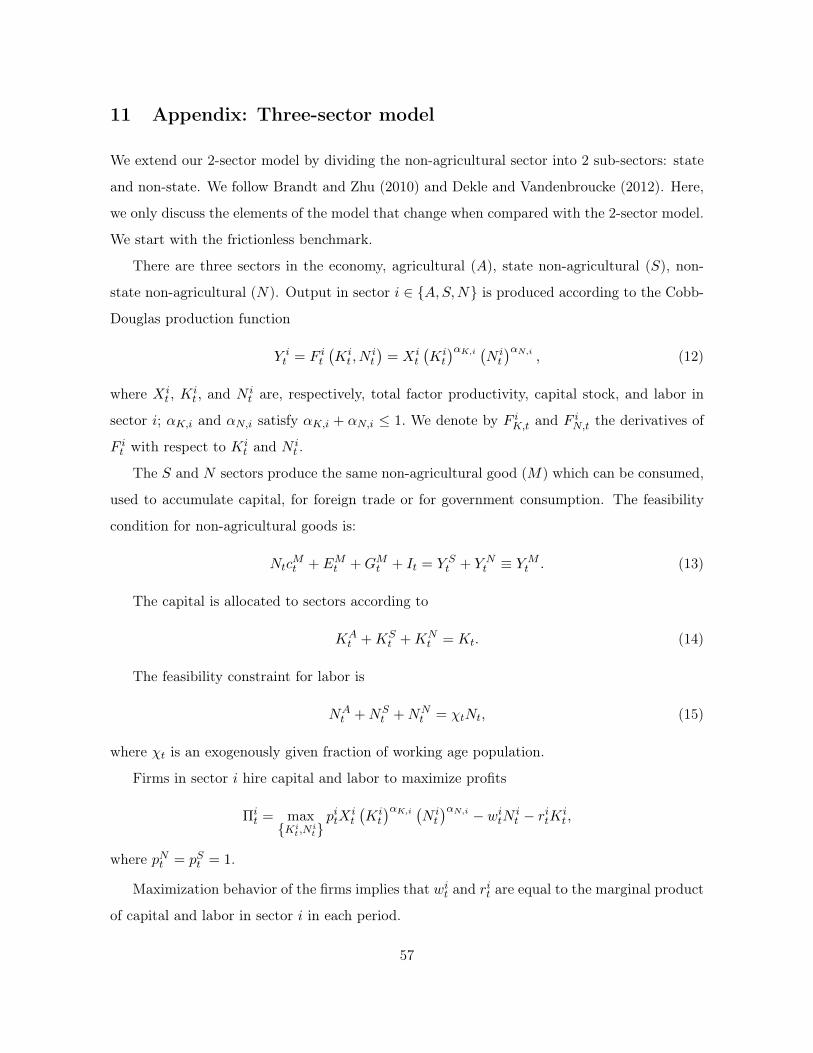
11 Appendix: Three-sector model

We extend our 2-sector model by dividing the non-agricultural sector into 2 sub-sectors: state

and non-state. We follow Brandt and Zhu (2010) and Dekle and Vandenbroucke (2012). Here,

we only discuss the elements of the model that change when compared with the 2-sector model.

We start with the frictionless benchmark.

There are three sectors in the economy, agricultural (A), state non-agricultural (S), non-

state non-agricultural (N). Output in sector i ∈ {A,S,N} is produced according to the Cobb-

Douglas production function

Y it = F it

(Kit , N

it

)= Xi

t

(Kit

)αK,i (N it

)αN,i , (12)

where Xit , K

it , and N i

t are, respectively, total factor productivity, capital stock, and labor in

sector i; αK,i and αN,i satisfy αK,i + αN,i ≤ 1. We denote by F iK,t and FiN,t the derivatives of

F it with respect to Kit and N i

t .

The S and N sectors produce the same non-agricultural good (M) which can be consumed,

used to accumulate capital, for foreign trade or for government consumption. The feasibility

condition for non-agricultural goods is:

NtcMt + EMt +GMt + It = Y S

t + Y Nt ≡ YM

t . (13)

The capital is allocated to sectors according to

KAt +KS

t +KNt = Kt. (14)

The feasibility constraint for labor is

NAt +NS

t +NNt = χtNt, (15)

where χt is an exogenously given fraction of working age population.

Firms in sector i hire capital and labor to maximize profits

Πit = max{Ki

t ,Nit}pitX

it

(Kit

)αK,i (N it

)αN,i − witN it − ritKi

t ,

where pNt = pSt = 1.

Maximization behavior of the firms implies that wit and rit are equal to the marginal product

of capital and labor in sector i in each period.

57

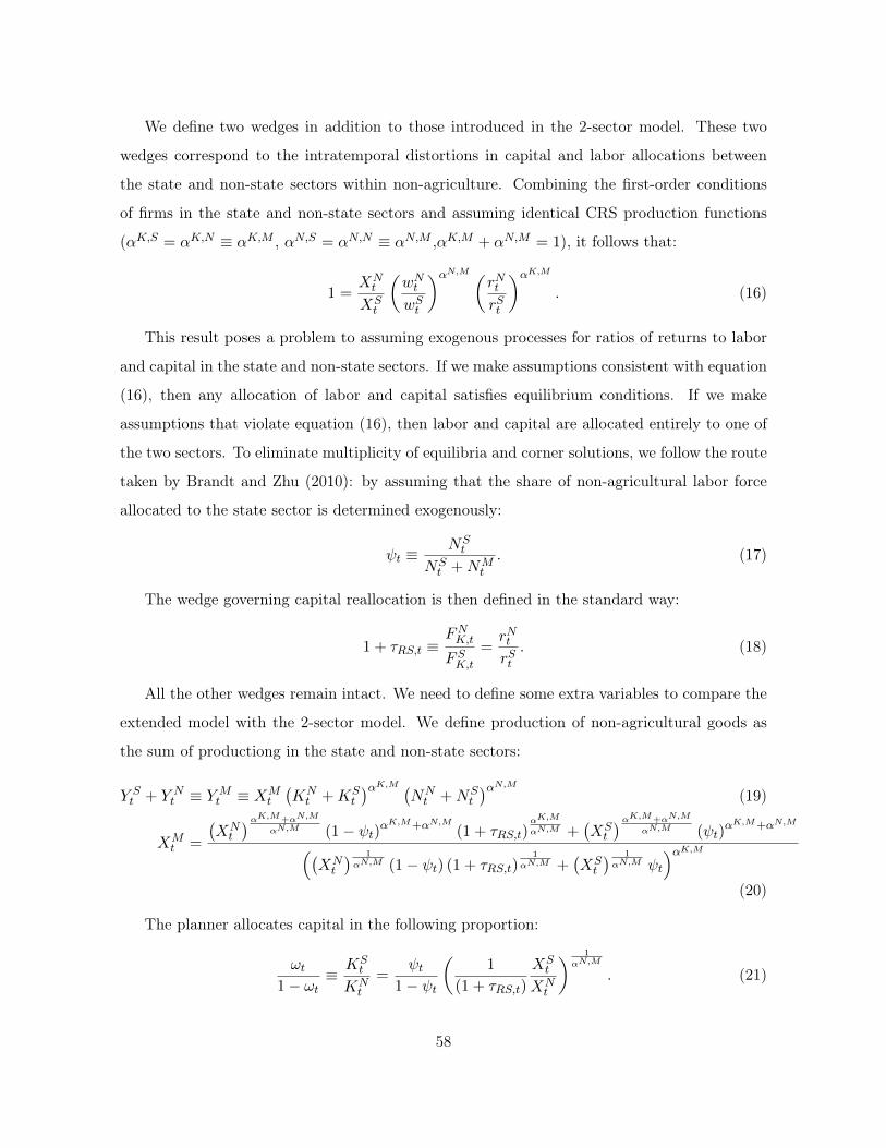
We define two wedges in addition to those introduced in the 2-sector model. These two

wedges correspond to the intratemporal distortions in capital and labor allocations between

the state and non-state sectors within non-agriculture. Combining the first-order conditions

of firms in the state and non-state sectors and assuming identical CRS production functions

(αK,S = αK,N ≡ αK,M , αN,S = αN,N ≡ αN,M ,αK,M + αN,M = 1), it follows that:

1 =XNt

XSt

(wNtwSt

)αN,M (rNtrSt

)αK,M. (16)

This result poses a problem to assuming exogenous processes for ratios of returns to labor

and capital in the state and non-state sectors. If we make assumptions consistent with equation

(16), then any allocation of labor and capital satisfies equilibrium conditions. If we make

assumptions that violate equation (16), then labor and capital are allocated entirely to one of

the two sectors. To eliminate multiplicity of equilibria and corner solutions, we follow the route

taken by Brandt and Zhu (2010): by assuming that the share of non-agricultural labor force

allocated to the state sector is determined exogenously:

ψt ≡NSt

NSt +NM

t

. (17)

The wedge governing capital reallocation is then defined in the standard way:

1 + τRS,t ≡FNK,t

FSK,t=rNtrSt. (18)

All the other wedges remain intact. We need to define some extra variables to compare the

extended model with the 2-sector model. We define production of non-agricultural goods as

the sum of productiong in the state and non-state sectors:

Y St + Y N

t ≡ YMt ≡ XM

t

(KNt +KS

t

)αK,M (NNt +NS

t

)αN,M (19)

XMt =

(XNt

)αK,M+αN,M

αN,M (1− ψt)αK,M+αN,M (1 + τRS,t)

αK,M

αN,M +(XSt

)αK,M+αN,M

αN,M (ψt)αK,M+αN,M((

XNt

) 1

αN,M (1− ψt) (1 + τRS,t)1

αN,M +(XSt

) 1

αN,M ψt

)αK,M(20)

The planner allocates capital in the following proportion:

ωt1− ωt

≡ KSt

KNt

=ψt

1− ψt

(1

(1 + τRS,t)

XSt

XNt

) 1

αN,M

. (21)

58

The wage differences between state and non-state sectors are determined as follows:

wNtwSt

=

(XSt

XNt

) 1

αN,M(

1

1 + τRS,t

)αK,M

αN,M

. (22)

Changes in τRS,t affect the allocation of capital, and also the relative returns to both capital

and labor. Changes in ψt determine the allocations of both capital and labor.

The returns to capital and labor in the non-agricultural sector are defined as:

rMt ≡α(Y Nt + Y S

t

)KMt

= ωtwSt + (1− ωt)wNt , (23)

wMt ≡β(Y Nt + Y S

t

)NMt

= ψtwSt + (1− ψt)wNt . (24)

Our analysis remains an accounting procedure. Given initial K0, competitive equilibrium

allocations with wedges{XNt , X

St , X

At , τ

Ct , τ

Pt , τ

Mt , τKt , τ

It , xt, qt, g

Mt , Nt, χt, τRS,t, ψt

}Tt=0

match

data exactly. This again allows to compute the marginal contribution of each wedge to the

deviations of data from undistorted allocations. all variables of interest.

59

12 Online Appendix: Sensitivity Analysis

In this section we consider the effects of alternative parameterizations of the model. The

baseline values for the parameters are presented in Table 2. We consider the effects of changes

in the key parameters: the production elasticities, the subsistence level and the elasticity of

substitution between goods — on two of our main results: wedge accounting for 1978-2012 and

the effect of reforms.

Tables 10-13 present the effects of parameter changes on the wedge accounting decompo-

sition of GDP growth and the change in the share of labor force in agriculture from 1978 to

2012. Similarly, Tables 14-17 present the effects of parameter changes on the effect of post-1978

reforms on GDP growth and the change in the share of labor force in agriculture.

We summarize the main effects as follows. First, a decrease in the degree of substitutability

between agricultural and manufacturing goods makes economic outcomes more sensitive to de-

velopments in the agricultural (subsistence) sector, and, hence, attributes more of the changes

in GDP and the share of labor force in agriculture to agricultural TFP and the distortion to

consumption, i.e. the consumption component of the intersectoral distortion. The contribu-

tions of other factors are diminished. Given that we deliberately chose a conservative value

of the elasticity of substitution in our baseline calibration, less substitutability between goods

(suggested by most micro estimates) only reinforces our main results.

Second, a substantial increase in the factor share of capital in the production function of

the non-agricultural sector decreases the contributions of TFPs and increases the contribution

of the mobility component of the intersectoral distortion. However, the overall effect of this

change in parameters is small. Third, the effects of changes in the factor shares of labor and

land in the agricultural production function are even smaller. An increase in the factor share

of labor implies a slightly bigger contribution of agricultural TFP while a decrease in the factor

share of land implies a slightly smaller contribution of agricultural TFP to changes in the share

of labor force in agriculture. The effects on contributions to GDP growth are negligible.

Fourth, the effects of changes in the subsistence level are more pronounced. A lower sub-

sistence level implies a smaller contribution of agricultural TFP and a bigger contribution of

intersectoral distortions. A higher subsistence level implies a larger contribution of agricultural

TFP and a smaller contribution of intersectoral distortions. Note that we deliberately set the

60

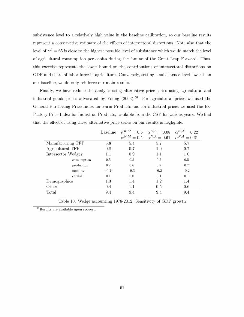
subsistence level to a relatively high value in the baseline calibration, so our baseline results

represent a conservative estimate of the effects of intersectoral distortions. Note also that the

level of γA = 65 is close to the highest possible level of subsistence which would match the level

of agricultural consumption per capita during the famine of the Great Leap Forward. Thus,

this exercise represents the lower bound on the contributions of intersectoral distortions on

GDP and share of labor force in agriculture. Conversely, setting a subsistence level lower than

our baseline, would only reinforce our main results.

Finally, we have redone the analysis using alternative price series using agricultural and

industrial goods prices advocated by Young (2003).50 For agricultural prices we used the

General Purchasing Price Index for Farm Products and for industrial prices we used the Ex-

Factory Price Index for Industrial Products, available from the CSY for various years. We find

that the effect of using these alternative price series on our results is negligible.

Baseline αK,M = 0.5 αK,A = 0.08 αK,A = 0.22αN,M = 0.5 αN,A = 0.61 αN,A = 0.61

Manufacturing TFP 5.8 5.4 5.7 5.7Agricultural TFP 0.8 0.7 1.0 0.7Intersector Wedges: 1.1 0.9 1.1 1.0

consumption 0.5 0.5 0.5 0.5production 0.7 0.6 0.7 0.7mobility -0.2 -0.3 -0.2 -0.2capital 0.1 0.0 0.1 0.1

Demographics 1.3 1.4 1.2 1.4Other 0.4 1.1 0.5 0.6Total 9.4 9.4 9.4 9.4

Table 10: Wedge accounting 1978-2012: Sensitivity of GDP growth50Results are available upon request.

61

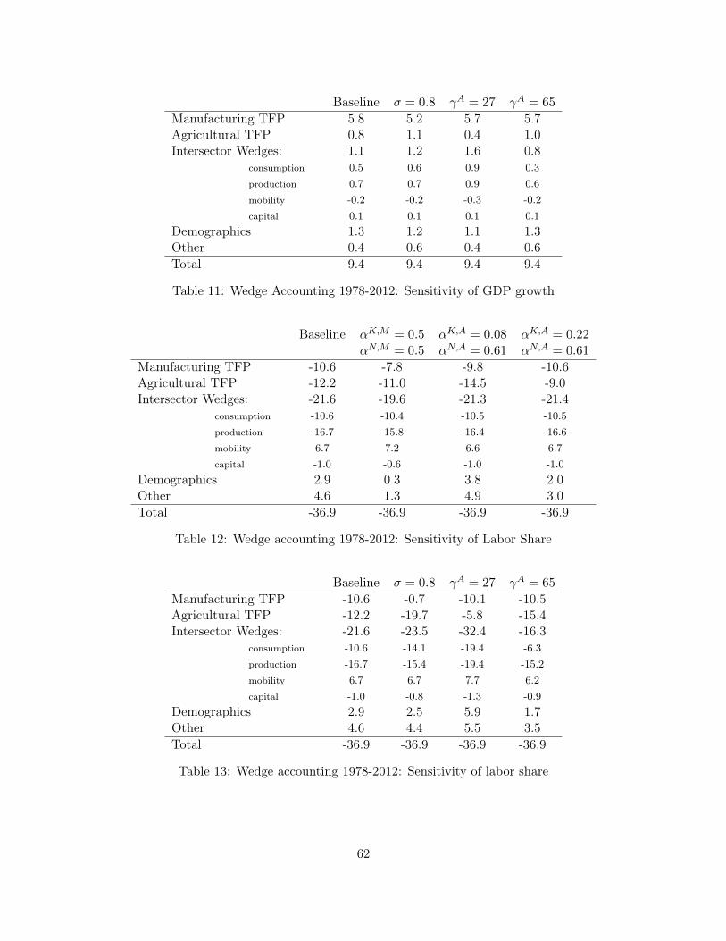
Baseline σ = 0.8 γA = 27 γA = 65

Manufacturing TFP 5.8 5.2 5.7 5.7Agricultural TFP 0.8 1.1 0.4 1.0Intersector Wedges: 1.1 1.2 1.6 0.8

consumption 0.5 0.6 0.9 0.3production 0.7 0.7 0.9 0.6mobility -0.2 -0.2 -0.3 -0.2capital 0.1 0.1 0.1 0.1

Demographics 1.3 1.2 1.1 1.3Other 0.4 0.6 0.4 0.6Total 9.4 9.4 9.4 9.4

Table 11: Wedge Accounting 1978-2012: Sensitivity of GDP growth

Baseline αK,M = 0.5 αK,A = 0.08 αK,A = 0.22αN,M = 0.5 αN,A = 0.61 αN,A = 0.61

Manufacturing TFP -10.6 -7.8 -9.8 -10.6Agricultural TFP -12.2 -11.0 -14.5 -9.0Intersector Wedges: -21.6 -19.6 -21.3 -21.4

consumption -10.6 -10.4 -10.5 -10.5production -16.7 -15.8 -16.4 -16.6mobility 6.7 7.2 6.6 6.7capital -1.0 -0.6 -1.0 -1.0

Demographics 2.9 0.3 3.8 2.0Other 4.6 1.3 4.9 3.0Total -36.9 -36.9 -36.9 -36.9

Table 12: Wedge accounting 1978-2012: Sensitivity of Labor Share

Baseline σ = 0.8 γA = 27 γA = 65

Manufacturing TFP -10.6 -0.7 -10.1 -10.5Agricultural TFP -12.2 -19.7 -5.8 -15.4Intersector Wedges: -21.6 -23.5 -32.4 -16.3

consumption -10.6 -14.1 -19.4 -6.3production -16.7 -15.4 -19.4 -15.2mobility 6.7 6.7 7.7 6.2capital -1.0 -0.8 -1.3 -0.9

Demographics 2.9 2.5 5.9 1.7Other 4.6 4.4 5.5 3.5Total -36.9 -36.9 -36.9 -36.9

Table 13: Wedge accounting 1978-2012: Sensitivity of labor share

62

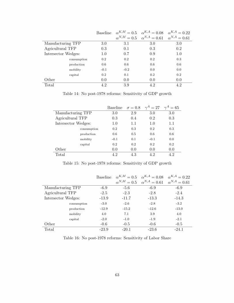
Baseline αK,M = 0.5 αK,A = 0.08 αK,A = 0.22αN,M = 0.5 αN,A = 0.61 αN,A = 0.61

Manufacturing TFP 3.0 3.1 3.0 3.0Agricultural TFP 0.3 0.1 0.3 0.2Intersector Wedges: 1.0 0.7 0.9 1.0

consumption 0.2 0.2 0.2 0.3production 0.6 0.6 0.6 0.6mobility -0.1 -0.2 0.0 0.0capital 0.2 0.1 0.2 0.2

Other 0.0 0.0 0.0 0.0Total 4.2 3.9 4.2 4.2

Table 14: No post-1978 reforms: Sensitivity of GDP growth

Baseline σ = 0.8 γA = 27 γA = 65

Manufacturing TFP 3.0 2.9 3.0 3.0Agricultural TFP 0.3 0.4 0.2 0.3Intersector Wedges: 1.0 1.1 1.0 1.1

consumption 0.2 0.3 0.2 0.3production 0.6 0.5 0.6 0.6mobility -0.1 0.1 -0.1 0.0capital 0.2 0.2 0.2 0.2

Other 0.0 0.0 0.0 0.0Total 4.2 4.3 4.2 4.2

Table 15: No post-1978 reforms: Sensitivity of GDP growth

Baseline αK,M = 0.5 αK,A = 0.08 αK,A = 0.22αN,M = 0.5 αN,A = 0.61 αN,A = 0.61

Manufacturing TFP -6.9 -5.6 -6.9 -6.9Agricultural TFP -2.5 -2.3 -2.8 -2.4Intersector Wedges: -13.9 -11.7 -13.3 -14.3

consumption -3.0 -2.6 -2.8 -3.2production -12.9 -15.2 -12.6 -13.0mobility 4.0 7.1 3.9 4.0capital -2.0 -1.0 -1.9 -2.1

Other -0.6 -0.5 -0.6 -0.5Total -23.9 -20.1 -23.6 -24.1

Table 16: No post-1978 reforms: Sensitivity of Labor Share

63

Baseline σ = 0.8 γA = 27 γA = 65

Manufacturing TFP -6.9 -5.8 -6.2 -7.1Agricultural TFP -2.5 -3.5 -1.5 -3.0Intersector Wedges: -13.9 -12.6 -13.3 -16.7

consumption -3.0 -2.4 -2.5 -5.1production -12.9 -9.4 -13.1 -13.7mobility 4.0 1.6 4.1 4.2capital -2.0 -2.4 -1.9 -2.2

Other -0.6 -0.5 -0.8 -0.5Total -23.9 -22.4 -21.8 -27.4

Table 17: No post-1978 reforms: Sensitivity of labor share

64