Embed Size (px)
Citation preview

The economics of motion perception and invariants ofvisual sensitivity
Perceptual Dynamics Laboratory Brain Science InstituteRIKEN Wakoshi Saitama JapanSergei Gepshtein
Perceptual Dynamics Laboratory Brain Science InstituteRIKEN Wakoshi Saitama Japan amp
Department of Mathematics University of LeicesterLeicester UKIvan Tyukin
Department of Psychology University of VirginiaCharlottesville VA USAMichael Kubovy
Neural systems face the challenge of optimizing their performance with limited resources just as economic systems doHere we use tools of neoclassical economic theory to explore how a frugal visual system should use a limited number ofneurons to optimize perception of motion The theory prescribes that vision should allocate its resources to differentconditions of stimulation according to the degree of balance between measurement uncertainties and stimulusuncertainties We find that human vision approximately follows the optimal prescription The equilibrium theory explainswhy human visual sensitivity is distributed the way it is and why qualitatively different regimes of apparent motion areobserved at different speeds The theory offers a new normative framework for understanding the mechanisms of visualsensitivity at the threshold of visibility and above the threshold and predicts large-scale changes in visual sensitivity inresponse to changes in the statistics of stimulation and system goals
Keywords uncertainty principle equilibrium visual sensitivity normative model optimality apparent motionmotion adaptation utility
Citation Gepshtein S Tyukin I amp Kubovy M (2007) The economics of motion perception and invariants of visualsensitivity Journal of Vision 7(8)8 1ndash18 httpjournalofvisionorg788 doi101167788
Introduction
Consider an organism that uses vision to estimate thespeeds of moving objects With unlimited resources itcould estimate the speeds by having a separate mechanismto measure each speed resulting in excellent precisionWith minimal resources it might have to make do with asingle mechanism to measure all speeds resulting in poorprecision How can the visual system find the rightbalance between frugality and precisionIn this article we find the balance using tools developed
in the neoclassical economic theory Our approach restson the notion of equilibrium introduced into the economictheory from mechanics (Pareto 1906) In economics thismethod allows one to find an optimal balance inconsumption of incommensurable goods (ldquoapples andorangesrdquo) for a customer or a market with a limitedbudget The allocation of resources to bundles of goods isoptimal when two conditions are met (1) Satisfactionfrom one component of the bundle cannot improvewithout reducing satisfaction from some other componentand (2) satisfaction from all the goods is the highestpossible Our analysis of motion perception using this
approach leads to equations of equilibrium very similar tothe equations in economics (Table 1) Now ldquoapples andorangesrdquo correspond to the parameters of optical stim-ulation and the ldquodegree of dissatisfactionrdquo corresponds tothe errorsVor the amount of uncertainty1Vin estimatingthe parameters (Gepshtein amp Tyukin 2006 GepshteinTyukin Kubovy amp van Leeuwen 2006) Just as aconsumer with limited financial resources seeks tominimize his or her dissatisfaction from a basket of fruitwe assume that vision with a limited pool of speed-tunedneurons seeks to minimize measurement errorsThe well-known fact that visual sensitivity to the
parameters of stimulation varies across the parameters isa manifestation of the differential allocation of visualresources A comprehensive summary of the visualsensitivity is the spatiotemporal contrast sensitivity func-tion (Kelly 1979 1994) We plot this function in thelogarithmic spacendashtime distance coordinates in Figure 1A(See Appendix A for details of its construction) In thisformat the different speeds are represented by the parallellines called speed lines In Figure 1A we show twocharacteristics of visual sensitivity the maximal sensitiv-ity set and the isosensitivity sets The maximal sensitivityset is represented by the grey hyperbolic curve that runs
Journal of Vision (2007) 7(8)8 1ndash18 httpjournalofvisionorg788 1
doi 10 1167 7 8 8 Received November 28 2006 published June 21 2007 ISSN 1534-7362 ARVO
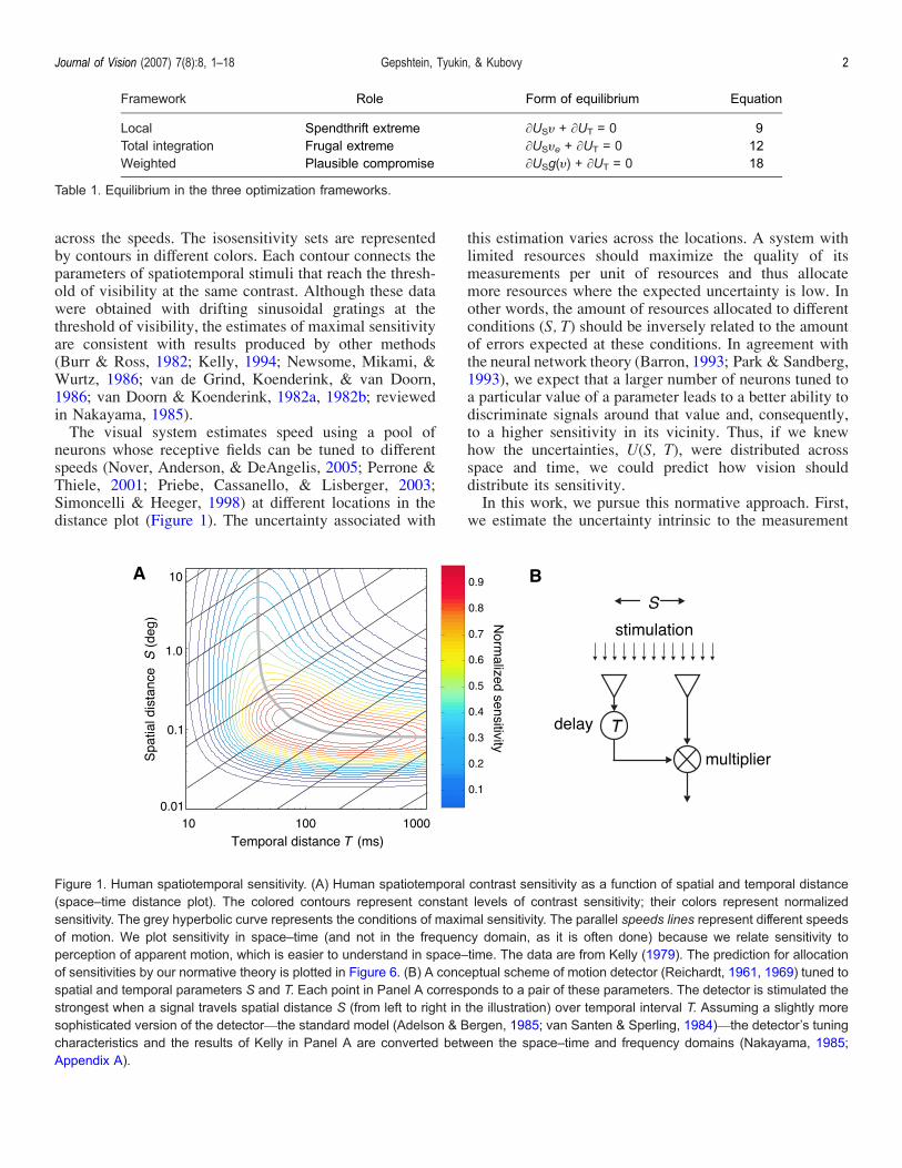
across the speeds The isosensitivity sets are representedby contours in different colors Each contour connects theparameters of spatiotemporal stimuli that reach the thresh-old of visibility at the same contrast Although these datawere obtained with drifting sinusoidal gratings at thethreshold of visibility the estimates of maximal sensitivityare consistent with results produced by other methods(Burr amp Ross 1982 Kelly 1994 Newsome Mikami ampWurtz 1986 van de Grind Koenderink amp van Doorn1986 van Doorn amp Koenderink 1982a 1982b reviewedin Nakayama 1985)The visual system estimates speed using a pool of
neurons whose receptive fields can be tuned to differentspeeds (Nover Anderson amp DeAngelis 2005 Perrone ampThiele 2001 Priebe Cassanello amp Lisberger 2003Simoncelli amp Heeger 1998) at different locations in thedistance plot (Figure 1) The uncertainty associated with
this estimation varies across the locations A system withlimited resources should maximize the quality of itsmeasurements per unit of resources and thus allocatemore resources where the expected uncertainty is low Inother words the amount of resources allocated to differentconditions (S T) should be inversely related to the amountof errors expected at these conditions In agreement withthe neural network theory (Barron 1993 Park amp Sandberg1993) we expect that a larger number of neurons tuned toa particular value of a parameter leads to a better ability todiscriminate signals around that value and consequentlyto a higher sensitivity in its vicinity Thus if we knewhow the uncertainties U(S T) were distributed acrossspace and time we could predict how vision shoulddistribute its sensitivityIn this work we pursue this normative approach First
we estimate the uncertainty intrinsic to the measurement
Framework Role Form of equilibrium Equation
Local Spendthrift extreme macrUSH + macrUT = 0 9Total integration Frugal extreme macrUSHe + macrUT = 0 12Weighted Plausible compromise macrUSg(H) + macrUT = 0 18
Figure 1 Human spatiotemporal sensitivity (A) Human spatiotemporal contrast sensitivity as a function of spatial and temporal distance(spacendashtime distance plot) The colored contours represent constant levels of contrast sensitivity their colors represent normalizedsensitivity The grey hyperbolic curve represents the conditions of maximal sensitivity The parallel speeds lines represent different speedsof motion We plot sensitivity in spacendashtime (and not in the frequency domain as it is often done) because we relate sensitivity toperception of apparent motion which is easier to understand in spacendashtime The data are from Kelly (1979) The prediction for allocationof sensitivities by our normative theory is plotted in Figure 6 (B) A conceptual scheme of motion detector (Reichardt 1961 1969) tuned tospatial and temporal parameters S and T Each point in Panel A corresponds to a pair of these parameters The detector is stimulated thestrongest when a signal travels spatial distance S (from left to right in the illustration) over temporal interval T Assuming a slightly moresophisticated version of the detectorVthe standard model (Adelson amp Bergen 1985 van Santen amp Sperling 1984)Vthe detectorrsquos tuningcharacteristics and the results of Kelly in Panel A are converted between the spacendashtime and frequency domains (Nakayama 1985Appendix A)
Table 1 Equilibrium in the three optimization frameworks
Journal of Vision (2007) 7(8)8 1ndash18 Gepshtein Tyukin amp Kubovy 2
of spatiotemporal signals (measurement uncertaintyGabor 1946) Second we predict at which locations inthe spacendashtime distance plot the conditions are mostfavorable for estimating speed taking into accountestimates of uncertainty about the speed of stimulation(stimulus uncertainty Dong amp Atick 1995) We startfrom constraints that apply to any measurement what-soever and deduce how the visual system might achievethe compromise between frugality and precision in faceof the uncertainties We find that the invariant propertiesof the optimal and uniformly suboptimal conditions formotion measurement predicted by the theory are similarto the maximal-sensitivity and isosensitivity conditionsfound in biological vision
Measurement uncertainty
Uncertainty principle of measurement
Consider receptive fields sensitive to a range of spatialand temporal frequencies $f 9 0 and a range of locationsin space and time $x 9 0 These ranges produceuncertainty with respect to the content2 and location of astimulus By the uncertainty principle of measurement(Gabor 1946 Resnikoff 1989) the product of theseuncertainties (spatial or temporal) cannot exceed apositive constant C1
$f $x Q C1 eth1THORN
In a system that is performing at its best (ie where $f $x = C1) one uncertainty cannot decrease without theother increasing Henceforth we will express the changesof uncertainty as equations and not as inequalities becauseour goal is to predict the best performance of the systemSuppose $f obeys the invariance of relative uncertainties
$f=f frac14 C2 eth2THORN
where C2 9 0 is a constant as it was shown for visualreceptive fields (eg Kulikowski Marcelja amp Bishop1982) This property represents a scale invariance ofmeasurement error similar to Weberrsquos law In contrast tothe generally valid uncertainty principle Equation 2summarizes empirical observations whose generality isnot confirmed Thus Equation 2 might serve as apostulateVor an assumptionVfrom which we derive thefunction describing how measurement uncertainties changeacross the conditions of stimulation (We relax thisassumption below) From Equations 1 and 2 it follows
$x frac14 C1=ethC2 f THORN$f frac14 C2 f
eth3THORN
Assuming additivity of uncertainties from Equation 3 wecan estimate how uncertainty changes across the entirerange of spatial or temporal parameters
U frac14 k1$x thorn k2$f frac14 k1C1
C2 f
thorn k2 C2 feth THORN eth4THORN
where $x is an interval of spatial or temporal locations($S or $T) $f is an interval of spatial or temporalfrequencies ($fS or $fT) and ki are unit coefficients thatbring the terms to the same units Equation 4 indicates thatthe measurement uncertainty varies as a composition ofdecaying and growing functions of frequency (Figure 1A)For a visual system that samples signals using Gabor
filters (ie filters obtained by multiplication of Gaussianand harmonic functions eg Daugman 1985 Jones ampPalmer 1987 MacKay 1981) we can estimate the shapeof uncertainty function without the assumption of invar-iance of relative uncertainties (Equation 2) Gabor (1946)showed that in such a system there exists a simplerelationship between the uncertainty in spacendashtime and infrequency domain (his Equation 127) We formulate thatrelationship in our terms as
$x frac14 1x= $f frac14 1f eth5THORNwhere corresponds to distance (spatial or temporalagainst which we plotted sensitivity in Figure 1A) and 1iare the weights (as in Equation 7 below) By addinguncertainties as we did in Equation 4 we again find thatthe composite uncertainty decays or grows as a function offrequency over different intervals of frequency (which isinversely related to ) Thus these features of thecomposite uncertainty function do not depend on theassumption of invariance of relative uncertainties
Spatiotemporal uncertainty function
By applying Equation 4 separately to spatial andtemporal uncertainties we derive the spatial and temporaluncertainty functions
US frac14 k1S $S thorn k2S $fS
frac14 k1SC1S
C2S fS
thorn k2S C2S fS
UT frac14 k1T $T thorn k2T $fT
frac14 k1TC1T
C2T fT
thorn k2T C2T fT
eth6THORN
By the assumption of additivity from Equation 6 weobtain the generalized spatiotemporal uncertainty function
UST STeth THORN frac14 US thorn UT US frac14 11Sthorn 13S
UT frac14 12Tthorn 14T eth7THORN
Journal of Vision (2007) 7(8)8 1ndash18 Gepshtein Tyukin amp Kubovy 3
where we converted fS and fT into S and T (Appendix A)and replaced the constants of Equation 6 and theconstants of the frequencyndashdistance conversion by con-stants 1i It is convenient to think of these constants as theweights expressing how much each term of Equation 7affects system goalsWe found that the shapes of predicted isosensitivity
contours which we derive in Figure 5 are similar to theshape of human isosensitivity contours in Figure 6 when13 and 14 were roughly two orders of magnitude greaterthan 11 and 12 The fact that the weights of termsconcerning localization in spacendashtime (13 14) are largein comparison with the weights of terms concerningfrequency identification (11 12) suggests that the spatio-temporal sensitivity function in Figure 6 reflects visualbehavior whose implicit goal has to do more with signallocalization than signal identificationIn Figure 2B we plot the spatial and temporal
uncertainty functions US and UT and the joint spatiotem-poral uncertainty function UST Each one-dimensional
uncertainty function on the side panels of Figure 2Bshows that uncertainties grow toward the high and lowends of each dimension The composition of uncertaintyfunctions is illustrated in Figure 2A
0 At the low end of each dimension small receptivefields allow precise estimation of signal location inspace or time (low values of Function A) but not inthe spatial or temporal frequency domains (highvalues of Function B)
0 In contrast at the high end of each dimension thereceptive fields allow the precise estimation of signallocation in the spatial or temporal frequency domains(low values of Function A) but not in space or time(high values of Function B)
Consequences of the additivity assumptions
In Equation 4 we assumed additivity of uncertaintiesbecause for a system at the optimal limit of its performance
Figure 2 Uncertainty functions (A) Functions A and B represent uncertainties associated with measuring the frequency content of signalsand localizing signals respectively Measurements of large spatial or temporal distances using large receptive fields suffer fromuncertainty about the location of signals in space or time (large values of function B at large distances) Measurements of small spatial ortemporal distances using small receptive fields suffer from uncertainty about the location of signals in the frequency domain spatialor temporal (large values of Function A at small distances) We describe the growth of uncertainty toward the extremes of spatial andtemporal dimensions of stimulation by assuming additivity of the small- and large-scale uncertainties (Function A + Function B)(B) Adding the spatial and temporal uncertainties (US and UT) in spacendashtime yields a spatiotemporal uncertainty function UST (US and UT
are shown on the side panels each is a replica of Function A + B in Panel A) The minimum of USTVglobal optimum OVand the levelcurves of UST are shown in a spacendashtime plot in the upper horizontal plane Shown in a spacendashtime plot in the lower horizontal plane arespeed lines which are parallel to each other in logarithmic coordinates The global optimum projects on one of the speed lines At thatpoint the estimates of speed are least affected by the uncertainties There are similarly optimal points on other speed lines these are thepoints where spatial and temporal uncertainties are in equilibrium (Figure 3 Table 1)
Journal of Vision (2007) 7(8)8 1ndash18 Gepshtein Tyukin amp Kubovy 4
multiplication of uncertainties within a dimension (spatial ortemporal) amounts to adding a constant (Equation 1) Therole of additivity in Equation 7 is different Multiplication ofspatial and temporal uncertainties in Equation 7 yields a newinseparable spacendashtime term in the uncertainty functionthis term does not change qualitatively significantpredictions of the theory (page 8)
Optimal conditions for speedestimation
The visual system would perform optimally if it usedsmall receptive fields to estimate location in spacendashtimeand large receptive fields to estimate location in the fre-quency domain perhaps using specialized subsystems toaccomplish different tasks But let us consider a frugalsystemwith scarce resources that cannot afford a separationto subsystems Such a system should compromise and usethe same receptive fields to measure several kinds of infor-mation minimizing the aforementioned uncertainties andalso trying to minimize the uncertainty of speed estimationThe measurement uncertainties described by the spatio-
temporal uncertainty function constrain the visual sys-temrsquos ability to estimate speed The effect of measurementuncertainty on speed estimation is smallest at the mini-mum of UST (red circle) in Figure 2 This global optimumfalls on one of the speed lines Because speed can bemeasured with least uncertainty at that point the visualsystem should allocate more resources for measuringspeed at that point than at any other point on this speedline But where are the similarly optimal conditions formeasuring other speedsBecause a straightforward answer to this question is
biologically implausible (as we show next) we answer itin two steps First we establish two extreme optimalityframeworks for speed estimation One is overly spend-thrift but estimates speed with infinite precision the otheris overly frugal but is imprecise at almost any speedSecond we find a principled balance between theseextremes and thus predict biologically plausible optimalconditions for the estimation of every speed
Local optimization A spendthrift extreme
We find an optimal condition on each speed linesimilar to the condition of global optimum by noting thatat the global optimum spatial and temporal uncertaintiesare exactly in balance A change in spatiotemporaluncertainty (dUST Equation 7) due to changes of US andUT is the total derivative of UST
dUST frac14 macrUS dSthorn macrUTdT eth8THORN
where macrUS = macrUSTmacrS and macrUT = macrUSTmacrT are the spatialand temporal partial derivatives of UST respectivelyBecause the spatial and temporal uncertainties balanceeach other where the total derivative is zero theequilibrium for every speed H = ST (which we write asdS = HdT for dT m 0) is
macrUSH thorn macrUT frac14 0 eth9THORNBy substituting US and UT from Equation 7 intoEquation 9 it follows that the conditions of equilibriumare satisfied by a hyperbola in the spacendashtime plot (graycurve in Figure 4)
S frac14ffiffiffiffiffiffiffiffiffiffiffiffiffiffiffiffiffiffiffiffiffiffiffiffiffiffiffiffiffiffiffiffiffiffiffiffiffiffi
11T2H
eth13H thorn 14THORNT2 j 12
s eth10THORN
As we show in Figure 3 the hyperbola for every speedpasses through two special points One is the globaloptimum (the orange circle) common to all the hyper-bolas the other is the local optimum for the speed (circlesmarked Oi in the insets) The latter point is unique formost speeds (Only for the speed whose speed line passesthrough the global optimum do the global and localoptima coincide Figure 3 inset A2)The optimal point on each speed line (local optimum) is
the intersection of the speed line and the hyperbolarepresenting the solution of the equation of balance ofuncertainties for that speed We find such balance pointson each speed line and thus discover the local optimal setfor estimating all the speeds it is shown as a thick blackcurve in Figure 3Note that we find the local minima in Equation 8 by
varying uncertainty functions in space and time (iebalancing dS and dT) rather than in the frequency domain(ie balancing dfS and dfT) because we are interested inthe optimal conditions for speed estimation rather than theoptimal conditions for measuring signalsrsquo frequencycontentsLocal optimization is biologically implausible for two
reasons
R1 Local optimization assumes that the visual systemcan tune its processing units for each speedindependent of other speeds This assumption mustbe false Any estimate of speed must involve somespatial and temporal integration because biologicalreceptive fields are extended in space and time
R2 Local optimization assumes that all speeds areequally important for perception This assumptionmust be false for two reasons (1) The distributionof speeds in the perceptual ecology is not uniform(Dong amp Atick 1995) and (2) some speeds aremore important to the organism than others
Journal of Vision (2007) 7(8)8 1ndash18 Gepshtein Tyukin amp Kubovy 5
Optimization by ldquototal integrationrdquoA frugal extreme
To understand how the integration across speeds inbiological vision affects the shape of the optimal set forspeed estimation we first consider an extreme caseintegration across all speeds This total-integration frame-work represents an overly frugal system whose resourcesare extremely limited and whose speed resolution is poorThe limiting case of such a system is the one with a singlespeed-tuned mechanism sensitive to the entire range ofspeedsTo find the optimal set predicted for the overly frugal
total-integration framework we integrate the contribution ofall speeds into the optimization process and use each speedrsquosprevalence in the perceptual ecology as a weight in theintegration The effect of weighting the contribution of eachspeed by its prevalence in the perceptual ecology is
dUI frac14Z V
0
pethHTHORNdUSTdH frac14 0
AacuteZ V
0
pethHTHORNethmacrUSH thorn macrUTTHORNdH frac14 0
eth11THORN
where p(H) is the distribution of speeds in the naturalstimulation (Dong amp Atick 1995) By rewriting the latterexpression as
Z V
0
pethHTHORN HdH
macrUS thornZ V
0
pethHTHORNdH
macrUT frac14 0 eth12THORN
taking into account the fact that X0Vp(H)dH = 1 and
introducing expected speed
He frac14Z V
0
pethHTHORN HdH eth13THORN
we obtain
macrUSHe thorn macrUT frac14 0 eth14THORN
Thus the integration yields an optimal set whosemathematical form is that of equilibrium (Table 1)The total-integration framework is not vulnerable to the
objections we raised about local optimization becausemany speeds contribute to the optimization process
Figure 3 Local optimization The local optimum for estimating speed Hi is intersection Oi of a hyperbola (which consists of points wherethe spatial and temporal uncertainties are balanced) and the speed line of Hi Insets A1ndashA3 show three such optima The set of all theintersections is the local optimal set shown as a thick black curve The orange circle is the point of global optimum of uncertainty fromFigure 2 The dashed line is the speed line that passes through global optimum
Journal of Vision (2007) 7(8)8 1ndash18 Gepshtein Tyukin amp Kubovy 6
(response to R1) and because the contribution of eachspeed is weighted by the distribution of speeds in theperceptual ecology (response to R2 in spirit of theBayesian approach Knill amp Richards 1996 Maloney2002 Weiss Simoncelli amp Adelson 2002) In theecological distribution low speeds are more likely thanhigh ones (Dong amp Atick 1995)The optimal set according to total integration is
invariantly a hyperbola in the distance plot the greycurve in Figure 4 Why a hyperbola As we saw inFigure 3 the conditions of equilibrium for each speedform a hyperbola in the spacendashtime distance plot(Equations 9 and 10) The local optimization frameworkcan afford finding the condition of equilibrium foreach speed Because multiple equilibriaVone perspeedVcontributed to the local optimal set the form ofthat set is generally different from hyperbolic In contrastthe total integration framework cannot access individualspeeds It can only estimate the weighted mean of all thespeeds that contribute to the integration The weightedmean of speed is the most likely speed in the perceptualecology the expected speed He Thus a single speeddominates optimization in this framework because ofwhich the optimal set is a single hyperbolaThis result that a single speed dominates optimization
in this framework is remarkable It means that the shapeof the distribution of speeds in the perceptual ecologymatters only inasmuch as it determines the mathematicalexpectation of that distribution the expected speed As we
show below a realistic compromise between the twoextreme optimization frameworks yields an optimal setvery similar to the set predicted by the total-integrationframework It is therefore the expected speed and not theshape of the distribution of speeds that controls theproperties of the optimal set predicted by our theoryNotice that the two extreme frameworksVlocal opti-
mization and total integrationVare dominated by differentuncertainties The spendthrift local-optimization frame-work can afford to allocate as much resources as needed tomeasure every speed so its optimal set depends only onU(S T) that is only on the measurement uncertainty Bycontrast the frugal total-integration framework mustallocate its resources carefully It must take into accountthe statistics of stimulationVthe stimulus uncertaintyVso itcan measure speed with optimal precision only at the mostlikely speed He The frugal framework is more sophisti-cated than the spendthrift one its optimal set is determinedby both the measurement and stimulus uncertainties
Weighted optimization A realisticcompromise
A realistic optimal set must lie between the spendthriftand the frugal The more limited the resources of asystem the more it should rely on stimulus uncertaintyand the more closely the optimal set should approach theprescription by frugal total integration On the other handthe more speed-tuned mechanisms a system can affordthe more such mechanisms it can allocate to the morecommon spatiotemporal parameters where stimulusuncertainty is relatively low Thus for speeds prevalentin the stimulation the optimal set should be closer to theset prescribed by local optimization than for other speedsTherefore the optimal strategy for resource allocationacross speeds depends on stimulus uncertainty If a speedis likely (low stimulus uncertainty) its optimal pointsshould be closer to the prediction of local optimization Ifa speed is unlikely (high stimulus uncertainty) its optimalpoints should be closer to the prediction of totalintegrationWe model this compromise by taking a linear combi-
nation of the conditions for optimization for the local(dUST) and total-integration (dUI) frameworks
wethHTHORNdUSTethHTHORN thorn frac121jwethHTHORNdUI frac14 0 eth15THORN
Remarkably this method of combination preserves theequilibrium of spatial and temporal uncertainties (Table 1)as we show nextThe effect of distribution of speeds p(H) on the
optimization of speed measurement depends on howprecisely visual mechanisms are tuned to speed In ourformulation of the maximal-sensitivity set in Equation 15precision of tuning is represented by the interval of
Figure 4 Three optimal sets for speed estimation The black curverepresents the local optimal set as in Figure 3 The greyhyperbola represents the total-integration optimal set The redcurve represents the weighted optimal set which is a realisticcompromise that falls between the two extreme sets At lowspeeds the realistic optimal set is closer to the local optimal setthan to the total-integration optimal set because low speedsprevail in the perceptual ecology
Journal of Vision (2007) 7(8)8 1ndash18 Gepshtein Tyukin amp Kubovy 7
integration across speeds the interval is denoted as W(H)below First we derive the integration intervals from theprinciple of uncertainty of measurement (as we did toobtain Equation 3) We find that the boundaries ofintegration should grow with speed Then we find theweight w(H) by integrating the contributions of differentspeeds over W(H)
wethHTHORN frac14ZethHTHORN
pethH1THORN dH1 eth16THORN
Boundaries of integration
We estimate the boundaries of integration intervals thesame way we have estimated the uncertainties associatedwith the spatial and temporal dimensions of stimulation(Equation 3) We rewrite Equation 2 in terms of spatialand temporal distances
$S=S frac14 CS
$T=T frac14 CTeth17THORN
where CS and CT are constants From this we estimate theinterval of uncertainty of speed Let ordfuaordf be the absoluteuncertainty (uncertainty pedestal) which does not dependon speed Then we write the lower (Ha) and upper (Hb)boundaries of the interval as
Ha frac14 jua thorn ethSj$STHORN=ethT thorn $TTHORNHb frac14 ua thorn ethSthorn $STHORN=ethTj$TTHORN
eth18THORN
where the first equation describes the minimal value ofmeasurement with an error in spatial and temporalestimates and the second equation describes the maximalvalue of such measurement We consider only the positivevalues of the intervalrsquos boundaries Because speed H = ST
Ha frac14 jua thorn Heth1jCSTHORN=eth1thorn CTTHORNHb frac14 ua thorn Heth1thorn CSTHORN=eth1jCTTHORN
hence HbjHa frac14 2ua thorn 2HethCS thorn CTTHORN=eth1jCT2THORN
eth19THORN
Thus interval W(H) = [Ha Hb] grows linearly with speed
Integration
By the integration over the variable interval W(H) wefind weights w(H) for Equation 15 and thus determine therealistic optimal set
macrUSgethHTHORN thorn macrUT frac14 0 eth20THORN
where g(H) = w(H) H + [1 j w(H)]He This set has a formsimilar to Equations 9 and 14 that is it also preserves theequilibrium of spatial and temporal uncertainties (Table 1)But now factor g(H) that modulates macrUS is a function ofspeedThe explicit form of this optimal set in the distance plot
is
S frac14ffiffiffiffiffiffiffiffiffiffiffiffiffiffiffiffiffiffiffiffiffiffiffiffiffiffiffiffiffiffiffiffiffiffiffiffiffiffiffiffiffiffiffi
11T2gethHTHORNeth13gethHTHORN thorn 14THORNT2j 12
s eth21THORN
which we plot as a red curve in Figure 4The realistic optimal set resembles the maximal-
sensitivity set of biological vision (Burr amp Ross 1982Kelly 1979 Nakayama 1985 Newsome et al 1986van de Grind et al 1986 van Doorn amp Koenderink1982a 1982b) in three ways
1 It is roughly a branch of a rectangular hyperbola in thefirst quadrant whose equation is of the form ST = constwhere S and T are spatial and temporal distancesrespectively The hyperbolic shape implies a tradingrelation between the spatial and temporal parameters
2 It approaches a vertical asymptote for low valuesof T
3 It deviates from a horizontal asymptote for highvalues of T predicted by local optimization
These similarities do not depend on the choice ofparameters of the spatiotemporal uncertainty function(Equation 6) and on the assumption of additivity of spatialand temporal uncertainties (Equation 7) Changing theparameters in Equation 6 results in changing the locationof the optimal set in the distance plot Abandoning theassumption of additivity amounts to having an inseparablespacendashtime term in the spatiotemporal uncertainty func-tion The weight of that term affects the curvature of theoptimal set in the transition between its vertical and nearlyhorizontal branches in the distance plot
Equally suboptimal conditionsfor speed estimation
We have characterized the visual systemrsquos optimalsensitivity to motion To characterize its performancewhen it is not at its best we derive equivalence sets ofuncertainty for speed estimation Just as the realisticoptimal set does these equivalence sets balance measure-ment uncertainty and stimulus uncertainty
Journal of Vision (2007) 7(8)8 1ndash18 Gepshtein Tyukin amp Kubovy 8
Measurement uncertainty Because the realistic optimalset represents a perfect balance of measurement uncertain-ties any point outside of it represents a degree of imbalanceof these uncertainties In Figure 5 we capture thisvariation of uncertainties using a curvilinear parametricgrid (Struik 1961) The curves for different degrees ofimbalance of measurement uncertainties form a family ofnonintersecting grid lines in the distance plot Each curvehas the roughly hyperbolic shape of the realistic optimalset The heavier curve H is the curve of exact balance Thefarther a curve of this grid is from H the greater imbalanceof measurement uncertainties it representsStimulus uncertainty Stimulus uncertainty is repre-
sented in Figure 5 by the linear part of the grey netformed by the speed lines The heavier line p is the speedline for the most likely speed He The farther a line of thisgrid is from p the less likely the corresponding speed is inthe perceptual ecologyWe find the conditions where the two kinds of
uncertainty are equally imbalanced by constructing circlesin the curvilinear system of the coordinates (Figure 5)We set a logarithmic scale on the two parametric grids inagreement with the theoretical and physiological consid-erations presented by Nover et al (2005) The details aredescribed in Appendix B We draw the family ofresulting equivalence sets in Figure 6A Independent ofthe choice of parameters the equivalence sets form closedcontours in the distance plot The shapes of contours
generally follow the invariantly hyperbolic shape of themaximal sensitivity set The theoretical equivalence setsare very similar to the observed ldquobent loaf-of-breadrdquoshape of human isosensitivity contours (Kelly 1994 ourFigure 1A)To summarize we have proposed that the visual system
should allocate its resources to the conditions of stimulationaccording to the uncertainty of speed estimation Thesimilarity between the theoretical optimal and equallysuboptimal sets to the empirical maximal sensitivity andisosensitivity sets supports this view and suggests that humanvision allocates its resources by the prescription of balancebetween uncertainties In agreement with the theory the visualsystem seems to allocate (a) more resources to the conditionsof stimulation where the different uncertainties are balancedexactly and (b) equal amount of resources to the conditionswith the same degree of imbalance of uncertainties
Discussion
Summary
We have developed a normative theory of motionperception We assumed that the visual system attemptsto minimize errors in estimation of motion speed But
Figure 5 Construction of an equivalence set Finding equivalence sets in a spacendashtime plot amounts to constructing a circle in thecurvilinear coordinate system shown as a gray net The coordinate system is the cartesian product of two parametric grids (1) curvilinearbalance grid which consists of curves of equal imbalance of spatial and temporal uncertainties and (2) linear speed grid which consistsof speed lines The axes are the line of expected speed H = He (marked p) and the optimal set by weighted optimization (marked H) Weconstruct an equivalence set by transforming coordinates p and H lt which results in a new coordinate system (p v) shown in the inset ltand then drawing a circle in (p v) The shape of the equivalence set is determined by mapping 8 of the circle from (p v) to the spacendashtime plot (Appendix B)
Journal of Vision (2007) 7(8)8 1ndash18 Gepshtein Tyukin amp Kubovy 9
biological vision with limited resources cannot optimizefor every speed We showed that in such a system the bestconditions for the estimation of speed are obtained whereuncertainties from different sources are balanced (ie arein equilibrium) These conditions form an optimal set forspeed estimation the invariantly hyperbolic shape of thisset is similar to the shape of the maximal sensitivity set ofhuman vision The equally suboptimal conditions forspeed estimation are obtained where uncertainties fromdifferent sources are imbalanced to the same degree Theconditions of equal imbalance form equivalence sets forspeed estimation the shapes of these sets are similar to theshapes of the isosensitivity sets of human visionWe used equilibrium analysis of uncertainties to explore
the consequences of very basic properties of visualmeasurement and considerations of biological parsimonyfor perception of motion Because our approach rests onvery basic considerations the predictions of the equili-brium theory are qualitative For example the theory doesnot predict the exact shapes of the isosensitivity contoursInstead the theory allows one to see that the peculiarbent-loaf-of-bread shape of human spatiotemporal sensi-tivity function plausibly manifests an optimal allocation oflimited neural resources In the following we illustrateseveral further consequences of our analysis We startfrom the theoretical equivalence sets and show that theinvariant shape of these sets helps to reconcile seemingly
inconsistent data on apparent motion Then we turn to thetheoretical optimal set and examine how its propertieschange in response to changes in the statistics ofstimulation and changes in system goals as well as whattestable predictions these changes entail
Apparent motion
From the shape of theoretical equivalence sets (Figure 6)it follows that spatial and temporal distances must interactdifferently under different conditions of stimulation toproduce equivalent condition for motion measurementWe illustrate this in Figure 6 using two pairs of conditionsshown as two pairs of connected circles ma ndash mb andmaVndash mbV3 Conditions within a pair correspond to the samedegree of imbalance between uncertainties because theybelong to the same equivalence set In thema ndash mb pair mb
is longer than ma in both space and time (coupling regime)whereas in themaV ndashmbV pairmbV is longer thanmaV in timebut shorter in space (tradeoff regime) Coupling obtainswhere the equivalence contours have positive slopes andtradeoff obtains where they have negative slopesIn fact both regimes of tradeoff and coupling were
observed in studies of apparent motion using supra-threshold stimuli But the difference between the twowas interpreted as a discrepancy between empirical
Figure 6 Equivalence contours (A) Theoretical equivalence sets (derived as explained in Figure 5 and Appendix B) We refer to thegraphic representation of the equivalence sets as equivalence contours The equivalence contours reproduce the ldquobent-loaf-of-breadrdquoshape of human isosensitivity contours (Panel B) The two pairs of connected circles (ma ndash mb and maV ndash mbV) demonstrate that differentregimes of spacendashtime combination are expected under different conditions of stimulation In the ma ndash mb pair equivalent conditions areobtained by increasing both spatial and temporal distances from ma to mb (spacendashtime coupling supporting Kortersquos third law of motion)In the maV ndash mbVpair equivalent conditions are obtained by increasing temporal distance and decreasing spatial distance (spacendashtimetradeoff contrary to Kortersquos law) (B) Human isosensitivity contours from Figure 1A
Journal of Vision (2007) 7(8)8 1ndash18 Gepshtein Tyukin amp Kubovy 10
findings rather than a manifestation of an optimal behaviorof the visual system
0 Spacendashtime coupling corresponds to Kortersquos (1915)venerable third law of motion (Koffka 19351963Lakatos amp Shepard 1997 Neuhaus 1930) Kortepresented his observers with two flashes separated byvariable spatial and temporal distances He first foundthe distances that gave rise to a compelling experi-ence of motion (ldquogood motionrdquo) But he found that hecould not change just the spatial distance or just thetemporal distance without reducing the strength ofmotion To restore the experience of good motion hehad to increase or decrease both
0 Evidence of spacendashtime tradeoff was found by Burtand Sperling (1981) who used ambiguous apparentmotion displays in which motion could be seen inone of several directions (ldquopathsrdquo) in the samestimulus When the authors varied the spatial andtemporal distances in their display they found thatthey had to decrease one distance and increase theother to maintain the equilibrium between theperception of different paths
Gepshtein and Kubovy (2007) reproduced bothresultsVcoupling and tradeoffVusing the same supra-threshold stimulus They showed that the qualitativelydifferent regimes of apparent motion are special cases of a
general pattern a smooth transition between the tradeoffand coupling as a function of speed (Figure 7) tradeoffoccurs at low speeds and coupling occurs at high speeds inagreement with predictions of the equilibrium theoryAccording to the theory the different regimes are observedunder different conditions of stimulation because the frugalvisual system balances the measurement and stimulusuncertainties associated with speed estimation
Motion adaptation
The equilibrium theory predicts changes in motionperception in response to changes in the statistics of speedin the stimulation because the properties of the optimal setfor speed estimation depend on the statistics Equation 20When vision is excessively stimulated with a single speedor a narrow band of speeds as it is often the case inmotion adaptation studies the equilibrium theory predictsthat sensitivity should change for the adapting speed(s)and also for speeds very different from the adapting oneRecall that the optimal set for speed estimation predictedby the theory is represented by a nearly hyperbolic curvein the distance plot (Figure 4) The position of this curve inthe distance plot depends on the most likely speed(expected speed He) in the stimulation (Equation 14) Ifchanges in statistics of stimulation change the expectedspeed then the optimal set for speed estimation shouldchange its position in the distance plot For example inFigure 8 we plot the preltadaptation optimal set computed
Figure 7 Empirical equivalence sets of apparent motion (A) The pairs of red connected circles represent the pairs of conditions ofapparent motion in perceptual equilibrium They were experienced equally often (Gepshtein amp Kubovy 2007) The thin black lines on thebackground are the empirical equivalence contours of apparent motion derived by Gepshtein and Kubovy (2007) from the pairwiseequilibria The slopes of both the empirical equivalence sets and the lines connecting the equilibrium pairs gradually change across theplot indicating a gradual change from the regime of tradeoff to the regime of coupling in qualitative agreement with measurements at thethreshold (Figure 1A copied to Panel B) and with the predictions of the equilibrium theory (Figure 6A) (B) Human isosensitivity contoursfrom Figure 1A The rectangle marks the region of conditions in which Gepshtein and Kubovy could measure the points of equilibrium ofapparent motion
Journal of Vision (2007) 7(8)8 1ndash18 Gepshtein Tyukin amp Kubovy 11
for an expected speed He and the postltadaptation optimalset computed for an adapting speed Ha Because of thechange in the position of the optimal set visual sensitivityis expected to change across a wide range of speeds moreso at high speeds where speed-specific optimizationoperates across wider range of speeds than at low speeds(Equation 19)Against the intuition and contrary to what is commonly
expected in the motion adaptation literature (reviewed inClifford ampWenderoth 1999 and Krekelberg VanWezel ampAlbright 2006) the equilibrium theory predicts that visualperformance will both improve and deteriorate at theadapting speed depending on where it is measured on thespeed line Ha The point of optimal sensitivity will movealong the speed line toward the prediction by localoptimization Visual sensitivity is expected to improve onthe part of the speed line that is close to the local optimumbut deteriorate in the vicinity of its preadaptation optimumfor most magnitudes of adapting speeds For example inFigure 8 an improvement of sensitivity is expected at thecondition marked by the green circle and a deteriorationis expected at the condition marked by the green squareAn exception from this pattern of changes is the regionof global optimum (the intersection of two curves in
Figure 8) where little change is expected independent ofthe magnitude of adapting speedThese predictions can be tested by measuring spatiotem-
poral sensitivity across a wide range of parameters to obtaina comprehensive characteristic of sensitivity (Figure 1A)before and after adaptation Such measurements will showwhether changes in sensitivity occur globally (ie atspeeds different from the adapting speed) and whether theglobal changes follow the pattern predicted by theequilibrium theory To our knowledge no such compre-hensive studies have been undertaken But data fromprevious motion adaptation studies suggest that changesin spatiotemporal sensitivity following adaptation areglobal For example Krekelberg et al (2006) studiedchanges in the responsiveness of speed-tuned cells in thecortical area MT of behaving monkeys It was found thatthe susceptibility of a cell to short-term adaptationdepended on whether the adapting speed was at the cellrsquosoptimum speed When the adapting speed was at the cellrsquosoptimum the effect of adaptation was often smaller thanwhen the adapting speed was different from the cellrsquosoptimum Krekelberg et al also found that when theadapting speed was at the cellrsquos optimum discriminationperformance sometimes improved and sometimes deter-iorated as we anticipated in Figure 8 To test whetherthe pattern of changes in discrimination performancefollows the pattern predicted in Figure 8 the adaptingstimuli should be narrowly localized in the space ofparameters (The adapting stimuli of Krekelberg et al werebroadband)
System goals
As we mentioned above parameters 1i of spatiotempo-ral uncertainty (Equation 7) can be thought of as weightsexpressing how much each of the uncertainty terms affectsthe precision of speed estimation The visual system canmodulate the effect of uncertainties on system behavior byredistributing its resources which in the present formu-lation of the equilibrium theory is equivalent to changingthe weightsThe terms of Equation 7 belong to two groups One
mostly affects the ability to localize signals (13S and 14T)and the other mostly affects the ability to identify signals(11S and 12T) Suppose that one of the two tasksVsignallocalization versus signal identificationVbecomes moreimportant to the visual system than the other Forexample consider an observer whose task is to discrim-inate the location of moving targets in the laboratory onone day and categorize moving targets by their spatialfeatures on another day By the equilibrium theory thevisual system will be able to improve its performance inone task at the expense of performance in the other taskby redistributing its resources Then predictable globalchanges in visual sensitivity are expected
Figure 8 Predicted consequences of motion adaptation The redand green lines represent expected speeds He of the natural(preltadaptation) environment (Equation 13) and Ha of the new(adapting) environment respectively As a result of adaptationthe optimal set for speed estimation changes from the onerepresented by the red curve (from Figure 4) to the onerepresented by the green curve The arrows indicate the directionof improvement of sensitivity along the two speed lines Thecircles and the squares on the speed lines mark examples ofconditions where sensitivity improves or deteriorates respectivelyVisual sensitivity is expected to change across a wide range ofspeeds Thus sensitivity is expected to improve for someconditions on the red speed line away from the adapting speedbut here the improvement is expected at larger temporaldistances than on the adapting speed line
Journal of Vision (2007) 7(8)8 1ndash18 Gepshtein Tyukin amp Kubovy 12
Thus performance in the identification task willimprove when the visual system allocates less resourcesfor measuring stimulus location and more resources formeasuring its frequency content This change correspondsto decreasing weights 13 and 14 relative to weights 11 and12 in Equation 7 The changes in weights imply a changein the position of the optimal set in the distance plot(Figure 4) For example the emphasis on signal identi-fication (decreasing 13 and 14 relative to 11 and 12) willcause the optimal set defined by Equation 20 to moveaway from the origin of the distance plot But when theemphasis is on signal identification and 13 and 14increase relative to 11 and 12 the optimal set will movetoward the origin Changes in the position of thetheoretical optimal set imply large-scale changes in visualsensitivity across the distance plot because the theoreticalequivalence sets (Figure 5 and Appendix B) will changetheir positions as wellNotice that the equilibrium theory predicts distinct
changes in the pattern of visual sensitivity in response tochanges in statistics of speed (as in motion adaptation)and changes in system goals When statistics of speedchange the optimal set is expected to move along thedirection of maximal speed variation that is along thenegative diagonal of the distance plot from the rightbottom corner to the left top corner (Figure 8) Whensystem goals change the optimal set is expected to movealong the other diagonal the imaginary line connectingthe left bottom and the right top corners of the distanceplot (not shown in Figure 8)Notice also that by the equilibrium theory one cannot
use different tasks and expect to obtain quantitativelyconsistent evidence about the same sensitivity character-istic of the visual system Different tasks will inducechanges in the quantitative detail of the spatiotemporalsensitivity function The amount and time course of suchchanges are interesting topics for future research
Comparison to other normative models ofvision
Contemporary decision-theoretic models of perceptionand behavior have features that appear similar to ourapproach We will now review the similarities anddifferences between the approaches
Weak fusion
The ldquoweak fusionrdquo theory of cue combination (Clark ampYuille 1990 Landy Maloney Johnsten amp Young 1995Maloney amp Landy 1989 Yuille amp Bulthoff 1996)predicts that the nervous system combines differentestimates of a parameter of interest using a linearweighting rule similar to the linear weighting in ourEquation 15 The linear weighting of the weak-fusion
framework is derived from the maximum likelihoodprinciple (Yuille amp Bulthoff 1996) and is used toimplement the assumption that a goal of cue combinationis to maximize the precision (minimize uncertainty) of thecombined estimate In our theory linear weightingappears for other reasons it allows us to find a principledcompromise between two extreme cases of optimalresource allocation one in a system with minimalresources and the other in a system with infinite resourcesThe optimal sets in both cases are characterized by theequilibrium of spatial and temporal uncertainties We usethe linear weighting scheme because it is the simplest onewe found that preserves the equilibrium of spatial andtemporal uncertainties in the compromise optimal set(Table 1)
Bayesian inference
The weights that appear in Equation 15 depend on thedistribution of speeds in the perceptual ecology Our useof the statistics of speed resembles the use of expecteddistributions of parameter values in inferential theories ofperception (Knill amp Richards 1996) derived from theBayesian decision theory (Berger 1985 Maloney 2002)In such theories the probabilities of sensory estimates(ldquolikelihood functionsrdquo) and the probabilities of corre-sponding parameter values in the natural stimulation(ldquoprior distributionsrdquo) are combined by point-by-pointmultiplication following Bayesrsquo rule making the preva-lent values in the stimulation more likely to be perceivedthan the less common values Thus the factors thatdetermine predictions are generally defined in the spaceof estimated parameters In contrast our predictions arederived in a space whose dimensions are different fromthe space of estimated parameters Our predictions dependon measurement uncertainty in addition to stimulusuncertainty and the effects of the two kinds of uncertaintyare separable Thus in Figure 5 the ldquospeed gridrdquo dependson stimulus uncertainty and the ldquobalance gridrdquo depends onmeasurement uncertainty The separation of these twogrids means that adaptive changes in system behavior arenot reducible to changes along the dimension of estimatedparameters alone
Utility theories
Decision-theoretic models of perception and behavioruse the notion of utility (Bernoulli 1954 Kahneman ampTversky 2000 Luce amp Raiffa 1957 Stigler 1950) toaccount for the fact that different errors in sensoryestimation or movement execution affect behavior differ-ently The ldquocostsrdquo of different errors are usually representedby a utility function (Geisler amp Kersten 2002 MaloneyTrommershauser amp Landy 2007 TrommershauserMaloney amp Landy 2003) The use of these functions
Journal of Vision (2007) 7(8)8 1ndash18 Gepshtein Tyukin amp Kubovy 13
resembles the use of prior probability functions inBayesian inferential models The probabilities of possiblesensory estimates or movements are weighted by thecorresponding utilities In our theory concepts similar toutility play a role at two places
1 In our measurement uncertainty function (Equation 7)coefficients 1i represent the weights of the compo-nents of uncertainty function One can think of thecoefficients as the costs of measurement errors just asthe values of a utility function can be thought of ascosts of errors in sensory estimation As we argued inthe System goals section the visual system maychange the weights of the components of measure-ment uncertainty to optimize itself for different tasksThis will affect our predictions differently from howchanges in utilities affect predictions of decision-theoretic models
a Changing weights in Equation 7 will affect themeasurement uncertainty and not the stimulusuncertainty The predicted changes will occuralong a dimension separate from the dimension ofstimulus uncertainty (As we explained in theBayesian inference section the effects of meas-urement uncertainty and stimulus uncertainty inour theory are separable)
b Changing weights in Equation 7 will affect thevisual sensitivity of the visual system whereaschanging utility functions in the decision-theoreticmodels will affect visually guided behavior at alater stage It is plausible that weighting oferrors in the nervous system happens both early(as implied by our theory) and late (as impliedby the decision-theoretic models) But the two kindsof weighting are expected to occur in differentparameter spaces The effects of early weightingwilloccur along the dimension of measurement uncer-tainty whereas the effects of late weighting willoccur in the space of estimated parameters Thesedifferences will allow one to experimentally separatethe effects of early and late weighting of errors
2 In our discussion of the limitations of the local-optimization approach we noted that both the speedprevalence and the importance of speeds for theorganism should affect motion perception (claim R2in the Local optimization A spendthrift extremesection) In the present work we used only theestimates of speed prevalence because to our knowl-edge no estimates of a speed ldquoimportance functionrdquoexist The effect of speed importance on equilibriumtheory predictions can be studied by modifying theexpression for p(H) in Equations 13 and 16 and in thederivation of the equivalence sets (Appendix B)
Conclusions
The equilibrium theory of speed estimation offers aprincipled explanation of the distribution of human visualsensitivity and explains why qualitatively differentregimes of apparent motion are observed at differentspeeds On this view the shapes of the empirical maximalsensitivity set and the isosensitivity sets (measured at thethreshold of visibility) and the different regimes ofapparent motion (measured above the threshold) aremanifestations of the optimal balance of uncertainties in avisual system that seeks to maximize the precision of itsmeasurements with limited resources Thus the equilibriumtheory offers a normative framework for understandingmotion perception at the threshold of visibility and above thethreshold and predicts how the visual system should adjustits sensitivity in response to changes in the statistics ofstimulation and changes in system goals
Appendix A
Construction of Figure 1
To display the isosensitivity contours in the spacendashtimedistance plot we use Equations 5ndash8 of Kelly (1979) withwhich he fit the spatiotemporal thresholds for thedetection of drifting sinusoidal gratings FollowingNakayama (1985 p 637) we computed the spatial andtemporal distances between successive discrete stimulithat correspond to Kellyrsquos spatial and temporal frequen-cies Nakayama assumed that motion is detected by pairsof spatial-frequency filters (ldquoquadrature pairsrdquo Adelson ampBergen 1985 Gabor 1946) in agreement with physio-logical (Marcelja 1980 Pollen amp Ronner 1981) andcomputational (Sakitt amp Barlow 1982) evidence The twoparts of such a detector are tuned to the same spatialfrequency fs but their spatial phases differ by 2 aquarter of the spatial period of the optimal stimulus (seealso van Santen amp Sperling 1984) When such a detectoris stimulated by a luminance grating with spatial fre-quency fs a spatial shift by S = 1 (4fs) will activate thedetector optimally Similarly the optimal temporal inter-val T of a detector is equal to the quarter period of itsoptimal temporal modulation T = 1 (4fT) By thisargument there exists a simple correspondence betweenthe frequency tuning of motion detectors and the spatialand temporal distance between successive stimuli thatactivate the detectors optimally Using the above expres-sions for S and T we mapped Kellyrsquos spatiotemporalthreshold surface (his Figure 15) to the logarithmic spacendashtime distance plot in Figure 1A In the distance plot themaximal sensitivity set is convex toward the origin Whenplotted in the coordinates of spatial and temporal
Journal of Vision (2007) 7(8)8 1ndash18 Gepshtein Tyukin amp Kubovy 14
frequencies as in Kellyrsquos Figure 15 the maximalsensitivity set is concave toward the originWe use the estimates of spatiotemporal sensitivity
obtained by Kelly (1979) from measurements using animage stabilization technique that afforded precise controlover retinal motion Those data had the same form asthe data obtained with no image stabilization (Kelly1969 1972 Kulikowski 1971 Robson 1966 van NesKoenderink Nas amp Bouman 1967) as Kelly andBurbeck (1984) observed This allows us to relate theestimates of Kelly (1979) to results from studies that didnot use image stabilization
Appendix B
Derivation of the equivalence sets(Figures 5 and 6)
We derived equivalence sets for speed estimation using acurvilinear system of coordinates (the grey net in Figure 5)embedded in the distance plot The system consists of twoparametric grids a curvilinear grid p that parameterizesmeasurement uncertainty and a linear grid H that parameter-izes stimulus uncertainty An equivalence set consists ofthe loci in coordinate system (p H) that are equidistant fromthe origin of (p H) That is an equivalence set is a circlein the curvilinear coordinates We illustrated that in theinset of Figure 5 by transforming (p H) into a rectilinearcoordinate system (p v)We constructed circles in (p H) in two steps
1 ParameterizationWe parameterized (p H) as follows
H For H we set the origin to He because by Equation14 the a priori uncertainty about speed is minimalwhen H = He We used a logarithmic scale assuggested by Nover et al (2005) The logarithmicscale leads to Weberrsquos law for speed discriminationthresholds (McKeeampWatamaniuk 1994 Nover et al2005) Also the logarithmic scale allowed us toparameterize speeds from the interval [0 V] tointerval [jV V] Thus we defined the scalingfunction
vethHTHORN frac14 lnethH=HeTHORN1=kH ethB1THORN
where kH is a constant
p If the optimal set represents perfect balance anequivalence set shares a degree of imbalance Henceto construct grid p we generalized Equation 20
macrUSgethHTHORN thorn macrUT frac14 p ethB2THORN
where p is the degree of imbalance We set the originof grid of p to zero because at p = 0 the solution ofEquation B2 is the optimal set The optimalsolutions of Equation B2 are feasible only below aboundary value of p that depends on speed pmax(H) =13 g(H) + 14 Because we had no a natural scale forp (in contrast to the scale for H) we assumed alogarithmic scaling function as we did for H
pethpTHORN frac14 lneth1jp=BTHORNj1=kp ethB3THORN
where kp is a constant B = 1 for p Z [jV 0] andB = pmax(H) for p 9 0 The choice of the logarithmicfunction did not affect the invariant properties of theequivalence sets (Figure 6)Vtheir closedness andhyperbolic shapeVand their similarity to humanisosensitivity contours (Figure 1A)
This parametrization results in a rectangular coordinatesystem (p v) shown in the inset of Figure 5
2 Mapping An equivalence set is a circle in (p v)centered on (p(0) = 0 v(He) = 0) We illustrate thisin Figure 5 for one point as mapping 8 of a pointfrom (p v) (in the inset) to a point in the spacendashtimeplot (in the main panel) From Equations 7 and 20 itfollows that the coordinates of a point (p = pV H = HV)in (S T) are
S frac14ffiffiffiffiffiffiffiffiffiffiffiffiffiffiffiffiffiffiffiffiffiffiffiffiffiffiffiffiffiffiffiffiffiffiffiffiffiffiffiffiffiffiffiffi
11T2gethHVTHORN
ethpmaxethHVTHORNjpVTHORNT2 j 12
s
T frac14 S=HV
8gtltgt ethB4THORN
(Note that the first equation is a generalization ofEquation 10) For a point (pV HV) we used Equation B4to find the coordinates of (pW HW) in (S T) for allpoints whose distance from (p = 0 v = 0) wasconstant such that ordfordfp(pV) v(HV)ordfordf=ordfordfp(pW) v(HW)ordfordfThus the solution of Equation B4 constitutes themapping 8 (p v) Y (S T)
Acknowledgments
We thank Wilson S Geisler and Michael S Landy fordiscussions Thomas D Albright Cees van Leeuwen andSergey Savelrsquoev for comments about an earlier version ofthis article and Peter Jurica for help in simulations of thenormative theory Parts of this work were presented at the
Journal of Vision (2007) 7(8)8 1ndash18 Gepshtein Tyukin amp Kubovy 15
5th Vision Sciences Society meeting (May 2006 SarasotaFL USA) and the 4th Asian Conference on Vision (July2006 Matsue Shimane Japan) Michael Kubovy wassupported by NEI Grant R01 EY12926 and NIDCD GrantR01 DC005636
Commercial relationships noneCorresponding author Sergei GepshteinEmail sergeibrainrikenjpAddress Perceptual Dynamics Laboratory Brain ScienceInstitute RIKEN Wakoshi Saitama Japan
Footnotes
1
Clarification of terms In measuring parameters ofstimulation (such as speed) a measurement error is thedifference between an estimate and the true value of theparameter of interest Measurement errors characterizeuncertainty about the parameter value Multiple measure-ments generally yield estimates that differ from oneanother and from the true value of the parameter Themore dispersed the distribution of these errors thegreater the uncertainty and the lower the precision ofestimation In sensory estimation different parametervalues correspond to different conditions of stimulationWe describe this by saying that the uncertainty andprecision of estimation vary across the conditions ofstimulation
2
Analysis of the spatial-frequency content of stimuli isimportant for perception of motion for two reasons Firstthe visual system needs to identify moving objectsPerformance in the identification task depends on ananalysis of spatial-frequency content of stimulation (DeValois amp De Valois 1990) Second the visual systemneeds to solve the motion matching problem (Hildreth1984 Ullman 1979) and the ability to solve it dependson the ability to measure the spatial-frequency content ofstimulation Motion matching problem is particularlydifficult when (spatially) small receptive fields are usedbecause small regions of retinal image are not uniqueThey are similar to many other regions of the image andthe matching process produces many spurious matches Asimilar argument was proposed by Banks Gepshtein andLandy (2004) with respect to the binocular matchingproblem
3
Each point in the distance plot (Figure 1) can representa narrow-band visual stimulus In broad-band stimulisuch as the apparent motion displays used by Burt andSperling (1981) or Gepshtein and Kubovy (2007) a pointin the distance plot corresponds to the fundamental spatialand temporal frequencies contained in the stimulus orsimply to the spatial and temporal distances betweensuccessive dots
References
Adelson E H amp Bergen J R (1985) Spatiotemporalenergy models for the perception of motion Journalof the Optical Society of America A Optics and imagescience 2 284ndash299 [PubMed]
Banks M S Gepshtein S amp Landy M S (2004) Whyis spatial stereoresolution so low Journal of Neuro-science 24 2077ndash2089 [PubMed] [Article]
Barron A R (1993) Universal approximation bounds forsuperpositions of a sigmoidal function IEEE Trans-action on Information Theory 39 930ndash945
Berger J O (1985) Statistical decision theory andbayesian analysis (2nd ed) New York Springer
Bernoulli D (1954) Exposition of a new theory on themeasurement of risk Econometrica 22 23ndash36(Originally published in 1738 Translated by LouiseSommer)
Burr D C amp Ross J (1982) Contrast sensitivity athigh velocities Vision Research 22 479ndash484[PubMed]
Burt P amp Sperling G (1981) Time distance andfeature tradeltoffs in visual apparent motion Psycho-logical Review 88 171ndash195 [PubMed]
Clark J J amp Yuille A L (1990) Data fusion forsensory information processing systems NorwellMA Kluwer Academic Publishers
Clifford C W amp Wenderoth P (1999) Adaptation totemporal modulation can enhance differential speedsensitivity Vision Research 39 4324ndash4332 [PubMed]
Daugman J G (1985) Uncertainty relation for resolutionin space spatial frequency and orientation optimizedby two-dimensional visual cortical filters Journal ofthe Optical Society of America A Optics and imagescience 2 1160ndash1169 [PubMed]
De Valois R L amp De Valois K K (Eds) (1990)Spatial vision New York Oxford University Press
Dong D amp Atick J (1995) Statistics of natural time-varying images Network Computation in NeuralSystems 6 345ndash358
Gabor D (1946) Theory of communication Institution ofElectrical Engineers 93(Pt III) 429ndash457
Geisler W S amp Kersten D (2002) Illusions perceptionandBayesNature Neuroscience 5 508ndash510 [PubMed][Article]
Gepshtein S amp Kubovy M (2007) The lawfulperception of apparent motion Journal of Vision7(8)9 1ndash15 httpjournalofvisionorg789doi101167789 [PubMed] [Article]
Journal of Vision (2007) 7(8)8 1ndash18 Gepshtein Tyukin amp Kubovy 16
Gepshtein S amp Tyukin I (2006) Why do moving thingslook as they do Vision The Journal of the VisionSociety of Japan 18 64
Gepshtein S Tyukin I Kubovy M amp van Leeuwen C(2006) A Pareto-optimality theory of motion percep-tion [Abstract] Journal of Vision 6(6)577 577ahttpjournalofvisionorg66577 doi10116766577
Hildreth E C (1984) Measurement of visual motionCambridge MA MIT Press
Jones J P amp Palmer L A (1987) An evaluation ofthe two-dimensional Gabor filter model of simplereceptive fields in cat striate cortex Journal ofNeurophysiology 58 1233ndash1258 [PubMed]
Kahneman D amp Tversky A (Eds) (2000) Choicesvalues and frames New York Cambridge UniversityPress
Kelly D H (1969) Flickering patterns and lateralinhibition Journal of the Optical Society of America59 1361ndash1370
Kelly D H (1972) Adaptation effects on spatio-temporalsine-wave thresholds Vision Research 12 89ndash101[PubMed]
Kelly D H (1979) Motion and vision II Stabilizedspatio-temporal threshold surface Journal of theOptical Society of America 69 1340ndash1349 [PubMed]
Kelly D H (1994) Eye movements and contrastsensitivity In D H Kelly (Ed) Visual science andengineering (Models and applications) (pp 93ndash114)New York Marcel Dekker Inc
Kelly D H amp Burbeck C A (1984) Critical problemsin spatial vision Critical Reviews in BiomedicalEngineering 10 125ndash177 [PubMed]
Knill D C amp Richards W (Eds) (1996) Perception asBayesian inference Cambridge UK CambridgeUniversity Press
Koffka K (19351963) Principles of Gestalt psychologyNew York A Harbinger Book Harcourt Brace ampWorld Inc
Korte A (1915) Kinematoskopische Untersuchungen[Kinematoscopic investigations] Zeitschrift fur Psy-chologie 72 194ndash296
Krekelberg B van Wezel R J amp Albright T D(2006) Adaptation in macaque MT reduces perceivedspeed and improves speed discrimination Journal ofNeurophysiology 95 255ndash270 [PubMed] [Article]
Kulikowski J J (1971) Some stimulus parametersaffecting spatial and temporal resolution of humanvision Vision Research 11 83ndash93 [PubMed]
Kulikowski J J Marcelja S amp Bishop P O (1982)Theory of spatial position and spatial frequencyrelations in the receptive fields of simple cells in the
visual cortex Biological Cybernetics 43 187ndash198[PubMed]
Lakatos S amp Shepard R N (1997) Constraintscommon to apparent motion in visual tactile andauditory space Journal of Experimental PsychologyHuman Perception and Performance 23 1050ndash1060[PubMed]
Landy M S Maloney L T Johnston E B amp Young M(1995) Measurement and modeling of depth cuecombination In defense of weak fusion VisionResearch 35 389ndash412 [PubMed]
Luce R D amp Raiffa H (1957) Games and decisionsNew York Wiley
MacKay D M (1981) Strife over visual corticalfunction Nature 289 117ndash118 [PubMed]
Maloney L T (2002) Statistical decision theory andbiological vision In D Heyer amp R Mausfeld (Eds)Perception and the physical world (pp 145ndash189)New York Wiley
Maloney L T amp Landy M S (1989) A Statisticalframework for robust fusion of depth information InW A Pearlman (Ed) Visual communications andimage processing IV (vol 1199 pp 1154ndash1163)Proceedings of SPIE
Maloney L T Trommershauser J amp Landy M S(2007) Questions without words A comparisonbetween decision making under risk and movementplanning under risk In W Gray (Ed) Integratedmodels of cognitive systems (pp 297ndash313) NewYork Oxford University Press
Marcelja S (1980) Mathematical description of theresponses of simple cortical cells Journal of theOptical Society of America 70 1297ndash1300[PubMed]
McKee S P amp Watamaniuk S N J (1994) Thepsychophysics of motion perception In A T Smith ampR J Snowden (Eds) Visual detection of motion(pp 85ndash114) London UK Academic Press
Nakayama K (1985) Biological image motion process-ing A review Vision Research 25 625ndash660[PubMed]
Neuhaus W (1930) Experimentelle Untersuchung derScheinbewegung [Experimental investigation ofapparent movement] Archiv Fur die Gesamte Psy-chologie 75 315ndash458
Newsome W T Mikami A amp Wurtz R H (1986)Motion selectivity in macaque visual cortex IIIPsychophysics and physiology of apparent motionJournal of Neurophysiology 55 1340ndash1351 [PubMed]
Nover H Anderson C H amp DeAngelis G C (2005) Alogarithmic scale-invariant representation of speed inmacaque middle temporal area accounts for speed
Journal of Vision (2007) 7(8)8 1ndash18 Gepshtein Tyukin amp Kubovy 17
discrimination performance Journal of Neuroscience25 10049ndash10060 [PubMed] [Article]
Pareto V (1906) Manual of political economy NewYork Augustus M Kelley (1971 translation of 1927edition)
Park J amp Sandberg I W (1993) Approximation andradial-basis-function networks Neural Computation5 305ndash316
Perrone J A amp Thiele A (2001) Speed skills Measuringthe visual speed analyzing properties of primate MTneurons Nature Neuroscience 4 526ndash532 [PubMed][Article]
Pollen D A amp Ronner S F (1981) Phase relationshipsbetween adjacent simple cells in the visual cortexScience 212 1409ndash1411 [PubMed]
Priebe N J Cassanello C R amp Lisberger S G (2003)The neural representation of speed in Macaque areaMTV5 Journal of Neuroscience 23 5650ndash5661[PubMed] [Article]
Reichardt W (1961) Autocorrelation a principle of evalua-tion of sensory information by the central nervoussystem In W A Rosenbluth (Ed) Sensory communi-cation (pp 303ndash318) Cambridge MA MIT Press
Reichardt W (1969) Movement perception in insects InW Reichardt (Ed) Processing of optical data byorganisms and by machines (pp 465ndash493) LondonUK Academic Press
Resnikoff H L (1989) The illusion of reality New YorkSpringer-Verlag New York Inc
Robson J G (1966) Spatial and temporal contrast-sensitivity functions of the visual system Journal ofthe Optical Society of America 56 1141ndash1142
Sakitt B amp Barlow H B (1982) A model for theeconomical encoding of the visual image in cerebralcortex Biological Cybernetics 43 97ndash108 [PubMed]
Simoncelli E P amp Heeger D J (1998) A model ofneuronal responses in visual area MT VisionResearch 38 743ndash761 [PubMed]
Stigler G J (1950) The development of utility theoryJournal of Political Economy 58 307ndash327
Struik D J (1961) Lectures on classical differentialgeometry New York Dover
Trommershauser J Maloney L T amp Landy M S(2003) Statistical decision theory and the selection ofrapid goal-directed movements Journal of theOptical Society of America A Optics image scienceand vision 20 1419ndash1433 [PubMed]
Ullman S (1979) The interpretation of visual motionCambridge MA MIT Press
van de Grind W A Koenderink J J amp van Doorn A J(1986) The distribution of human motion detectorproperties in the monocular visual field VisionResearch 26 797ndash810 [PubMed]
van Doorn A J amp Koenderink J J (1982a) Spatialproperties of the visual detectability of movingspatial white noise Experimental Brain Research45 189ndash195 [PubMed]
van Doorn A J amp Koenderink J J (1982b) Temporalproperties of the visual detectability of moving spatialwhite noiseExperimental Brain Research 45 179ndash188[PubMed]
van Nes F L Koenderink J J Nas H amp Bouman M A(1967) Spatiotemporal modulation transfer in thehuman eye Journal of the Optical Society of America57 1082ndash1088 [PubMed]
van Santen J P amp Sperling G (1984) Temporalcovariance model of human motion perceptionJournal of the Optical Society of America A 1451ndash473 [PubMed]
Weiss Y Simoncelli E P amp Adelson E H (2002)Motion illusions as optimal percepts Nature Neuro-science 5 598ndash604 [PubMed]
Yuille A L amp Bulthoff H H (1996) Bayesian decisiontheory and psychophysics In D C Knill amp WRichards (Eds) Perception as Bayesian inference(pp 123ndash161) Cambridge UK Cambridge Univer-sity Press
Journal of Vision (2007) 7(8)8 1ndash18 Gepshtein Tyukin amp Kubovy 18
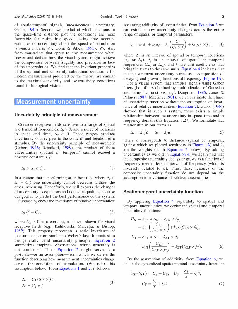
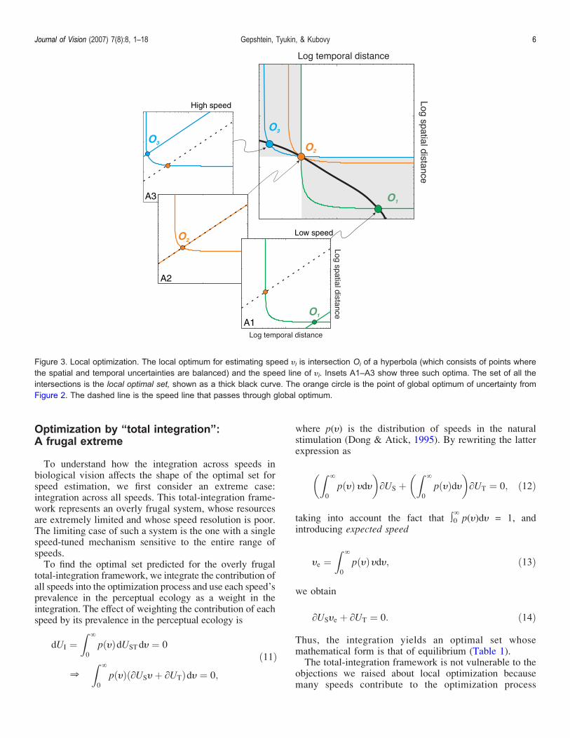