Embed Size (px)
Citation preview


Modern Birkhauser Classics
applied mathematics published by Birkhauser in recent decades havebeen groundbreaking and have come to be regarded as foundational tothe subject. Through the MBC Series, a select number of these modernclassics, entirely uncorrected, are being re-released in paperback (andas eBooks) to ensure that these treasures remain accessible to newgenerations of students, scholars, and researchers.
Many of the original research and survey monographs in pure and
and Hamiltonian DynamicsSymplectic Invariants
Reprint of the 1994 Edition
Helmut Hofer Eduard Zehnder

Printed on acid-free paper
Springer Basel AG is part of Springer Science+Business Media
www.birkhauser-science.com
Cover design: deblik, Berlin
c
¨
specifically the rights of translation, reprinting, re-use of illustrations, broadcasting, reproduction on microfilms
owner must be obtained.
This work is subject to copyright. All rights are reserved, whether the whole or part of the material is concerned,
or in other ways, and storage in data banks. For any kind of use whatsoever, permission from the copyright
Helmut HoferInstitute for Advanced Study (IAS)
Einstein DrivePrinceton, New Jersey 08540USA
Eduard Zehnder
ETH Zürich
Leonhardstrasse 27
ISBN 978-3-0348-0103-4 e-ISBN 978-3-0348-0104-1DOI 10.1007/978-3-0348-0104-1
© 1994 Birkhäuser Verlag
Birkhauser Verlag, Switzerland, ISBN 978-3-7643-5066-6Reprinted 2011 by Springer Basel AG
School of Mathematics
8092 Zürich
2010 Mathematics Subject Classification: 37-02, 54H20, 57R17, 58E05
Originally published under the same title in the Birkhäuser Advanced Texts - Basler Lehrbücher series by
Library of Congress Control Number: 2011924350
Departement Mathematik
Contents
1 Introduction1.1 Symplectic vector spaces . . . . . . . . . . . . . . . . . . . . . . . . 11.2 Symplectic diffeomorphisms and Hamiltonian vector fields . . . . . 61.3 Hamiltonian vector fields and symplectic manifolds . . . . . . . . . 91.4 Periodic orbits on energy surfaces . . . . . . . . . . . . . . . . . . . 181.5 Existence of a periodic orbit on a convex energy surface . . . . . . 231.6 The problem of symplectic embeddings . . . . . . . . . . . . . . . . 311.7 Symplectic classification of positive definite quadratic forms . . . . 351.8 The orbit structure near an equilibrium, Birkhoff normal form . . . 42
2 Symplectic capacities2.1 Definition and application to embeddings . . . . . . . . . . . . . . 512.2 Rigidity of symplectic diffeomorphisms . . . . . . . . . . . . . . . . 58
3 Existence of a capacity3.1 Definition of the capacity c0 . . . . . . . . . . . . . . . . . . . . . . 693.2 The minimax idea . . . . . . . . . . . . . . . . . . . . . . . . . . . 773.3 The analytical setting . . . . . . . . . . . . . . . . . . . . . . . . . 823.4 The existence of a critical point . . . . . . . . . . . . . . . . . . . . 913.5 Examples and illustrations . . . . . . . . . . . . . . . . . . . . . . . 98
4 Existence of closed characteristics4.1 Periodic solutions on energy surfaces . . . . . . . . . . . . . . . . . 1054.2 The characteristic line bundle of a hypersurface . . . . . . . . . . . 1134.3 Hypersurfaces of contact type, the Weinstein conjecture . . . . . . 1194.4 “Classical” Hamiltonian systems . . . . . . . . . . . . . . . . . . . 1274.5 The torus and Herman’s Non-Closing Lemma . . . . . . . . . . . . 137
5 R2n
5.1 A special metric d for a group D ofHamiltonian diffeomorphisms . . . . . . . . . . . . . . . . . . . . . 143
5.2 The action spectrum of a Hamiltonian map . . . . . . . . . . . . . 1515.3 A “universal” variational principle . . . . . . . . . . . . . . . . . . 1545.4 A continuous section of the action spectrum bundle . . . . . . . . . 1615.5 An inequality between the displacement energy
and the capacity . . . . . . . . . . . . . . . . . . . . . . . . . . . . 1655.6 Comparison of the metric d on D with the C0-metric . . . . . . . . 1735.7 Fixed points and geodesics on D . . . . . . . . . . . . . . . . . . . 182
v
Geometry of Compactly supported symplectic mappings in
vi Contents
6 The Arnold conjecture, Floer homology and symplectic homology6.1 The Arnold conjecture on symplectic fixed points . . . . . . . . . . 1946.2 The model case of the torus . . . . . . . . . . . . . . . . . . . . . . 2026.3 Gradient-like flows on compact spaces . . . . . . . . . . . . . . . . 2176.4 Elliptic methods and symplectic fixed points . . . . . . . . . . . . . 2226.5 Floer’s appraoch to Morse theory for the action functional . . . . . 2506.6 Symplectic homology . . . . . . . . . . . . . . . . . . . . . . . . . . 265
AppendixA.1 Generating functions of symplectic mappings in R
2n . . . . . . . . 273A.2 Action-angle coordinates, the Theorem of Arnold and Jost . . . . . 278A.3 Embeddings of H1/2(S1) and smoothness of the action . . . . . . . 286A.4 The Cauchy-Riemann operator on the sphere . . . . . . . . . . . . 291A.5 Elliptic estimates near the boundary and an application . . . . . . 298A.6 The generalized similarity principle . . . . . . . . . . . . . . . . . . 302A.7 The Brouwer degree . . . . . . . . . . . . . . . . . . . . . . . . . . 305A.8 Continuity property of the Alexander-Spanier cohomology . . . . . 314
Index . . . . . . . . . . . . . . . . . . . . . . . . . . . . . . . . . . . . . . . 321
Bibliography . . . . . . . . . . . . . . . . . . . . . . . . . . . . . . . . . . . 327

We dedicate this book to our friend
Andreas Floer
1956–1991

Preface
The discoveries of the past decade have opened new perspectives for the old field ofHamiltonian systems and led to the creation of a new field: symplectic topology.Surprising rigidity phenomena demonstrate that the nature of symplectic map-pings is very different from that of volume preserving mappings which raised newquestions, many of them still unanswered. On the other hand, due to the analysisof an old variational principle in classical mechanics, global periodic phenomena inHamiltonian systems have been established. As it turns out, these seemingly differ-ent phenomena are mysteriously related. One of the links is a class of symplecticinvariants, called symplectic capacities. These invariants are the main theme ofthis book which grew out of lectures given by the authors at Rutgers University,the RUB Bochum and at the ETH Zurich (1991) and also at the Borel Seminar inBern 1992. Since the lectures did not require any previous knowledge, only a fewand rather elementary topics were selected and proved in detail. Moreover, our se-lection has been prompted by a single principle: the action principle of mechanics.The action functional for loops in the phase space, given by
F (γ) =∫
γ
pdq −1∫
0
H(t, γ(t)
)dt ,
differs from the old Hamiltonian principle in the configuration space defined by aLagrangian. The critical points of F are those loops γ which solve the Hamiltonianequations associated with the Hamiltonian H and hence are the periodic orbits.This variational principle is sometimes called the least action principle. However,there is no minimum for F . Indeed, the action principle is very degenerate. Allits critical points are saddle points of infinite Morse index, and at first sight, theprinciple appears quite useless for existence proofs. But surprisingly it is very effec-tive. This will be demonstrated using several variational techniques starting fromminimax arguments due to P. Rabinowitz and ending with A. Floer’s homology.The book includes the following subjects:
The introductory chapter presents in a rather unsystematic way some back-ground material. We give the definitions of symplectic manifolds and symplecticmappings and briefly recall the Hamiltonian formalism. For convenience, Cartan’scalculus is used. The classification of 2-dimensional symplectic manifolds by theEuler-characteristic and the total volume is proved. Some questions dealt withlater on in detail are raised and discussed in special examples. We illustrate theso-called direct method of the calculus of variations in order to establish a periodicorbit on a convex energy surface of a Hamiltonian system in R
2n. The Birkhoffinvariants are introduced in order to describe without proofs the intricate orbit
ix
x Preface
structure of a Hamiltonian system near an equilibrium point or near a periodicsolution. These local results are quite in contrast to the global questions dealt within the following chapters.
In a systematic way the symplectic invariants, called symplectic capacities, areintroduced axiomatically in Chapter 2. Considering the family of all symplecticmanifolds of fixed dimension 2n, a capacity c is a map associating with every sym-plectic manifold (M,ω) a positive number c(M,ω) or ∞ satisfying these axioms:a monotonicity axiom for symplectic embeddings, a conformality axiom for thesymplectic structure, and a normalization axiom which rules out the volume inhigher dimensions. For subsets of R
2n, the capacity extends a familiar linear sym-plectic invariant for positive quadratic forms to nonlinear symplectic mappings.If M and N are symplectically diffeomorphic then c(M,ω) = c(N, τ). In view ofits monotonicity property a capacity represents, in particular, an obstruction tocertain symplectic embeddings and it will be used in order to explain rigidity phe-nomena for symplectic embeddings, discovered by Ya. Eliashberg and M. Gromov.In particular, Gromov’s squeezing theorem is deduced using capacities as well asEliashberg’s C0-stability of symplectic diffeomorphisms. We introduce a notionof a symplectic homeomorphism, a concept which raises many questions. Thereare many different capacity functions. For example, the size of the largest ballin R
2n which can be symplectically embedded into a symplectic manifold (M,ω)leads to a special capacity called the Gromov width. It is the smallest capacityfunction originally introduced by M. Gromov. There are many other “embedding”capacities.
Chapter 3 is devoted entirely to a very detailed construction of a distinguishedsymplectic capacity c0. It is dynamically defined by means of Hamiltonian systems.It measures the minimal C0-oscillation of a Hamiltonian function H : M → R
which allows to conclude the existence of a fast periodic solution of the corre-sponding Hamiltonian vector field XH on M . In the special case of a connected2-dimensional symplectic manifold, the capacity c0 agrees with the total area. Theexistence proof is based on the above action principle which is introduced fromscratch in its proper functional analytic framework. The interesting aspect of thisprinciple is that it is bounded neither from below nor from above so that stan-dard variational techniques do not apply directly. Techniques going back to P.Rabinowitz permit us to establish effectively distinguished saddle points of thefunctional representing special periodic solutions of the system. In the special caseof a convex, bounded and smooth domain U ⊂ R
2n, the capacity is represented bya distinguished closed characteristic of its boundary ∂U : it has minimal reducedaction equal to c0(U). But, in general, it is rather difficult to compute the invariantc0. Some of the recent computations based on more advanced techniques of firstorder elliptic systems and Fredholm theory are presented without proofs. With theconstruction of the capacity c0, the proofs of the rigidity phenomena described inChapter 2 are complete. Due to its special properties this invariant turns out tobe useful also for the dynamics of Hamiltonian systems.
Preface xi
In Chapter 4 the dynamical capacity c0 is applied to an old question of thequalitative theory of Hamiltonian systems originating in celestial mechanics: doesa compact energy surface carry a periodic orbit? We shall demonstrate that manywell-known global existence results previously obtained by technically intricateproofs emerge immediately from this invariant. The phenomenon is simply this:if a compact hypersurface in a symplectic manifold possesses a neighborhood offinite capacity c0, then there are always uncountably many closed characteristicsnearby. If one poses, in addition, symplectically invariant restrictions, such as of“contact type”, then the hypersurface itself carries a closed characteristic. Weshall prove, in particular, the seminal solution of the Weinstein conjecture in R
2n
due to C. Viterbo. A nonstandard symplectic torus shows that, in contrast tothe Gromov width mentioned above, not every compact symplectic manifold isof finite capacity c0. Our special example is related to M. Herman’s celebratedcounterexample to the closing lemma which answers a longstanding open questionin dynamical systems. M. Herman’s “non-closing-lemma” is proved at the end ofthe chapter.
In Chapter 5 we study the subgroup D of symplectic diffeomorphisms of R2n
which are generated by time dependent Hamiltonian vector fields of compact sup-port. The distance from the identity map or the energy E(ϕ) of such a symplecticdiffeomorphism ϕ will be measured by means of the oscillation of its generatingHamiltonian function. This will lead to a surprising bi-invariant metric on D calledthe Hofer metric and defined by d(ϕ,ψ) = E(ϕ−1 ψ). The definition does notinvolve derivatives of the Hamiltonian and is of C0-nature. The verification of themetric property requiring that d(ϕ,ψ) = 0 if and only if ϕ = ψ is the difficult as-pect. It is based on more refined minimax arguments for the action functional validsimultaneously for a large class of Hamiltonians. We shall investigate the relationsof this distinguished metric to the dynamical symplectic invariant c0 introducedin Chapter 3 and also to another symplectic invariant which is defined for subsetsof R
2n and called the displacement energy. The displacement energy of a subsetU measures the minimal energy E(ϕ) needed in order to dislocate a given set Ufrom itself in the sense that U ∩ ϕ(U) = ∅. The bi-invariant metric will also becompared with the standard sup-metric. Geodesic arcs associated with the metricwill be defined and described in detail. A special example of a geodesic arc is theflow generated by an autonomous Hamiltonian. An important role in our approachis played by the action spectrum of a Hamiltonian mapping ϕ ∈ D, which turnsout to be a nowhere dense subset of the real numbers. Our minimax principlesingles out a nontrivial continuous section of the action spectrum bundle over Dcalled the γ-invariant. This invariant is the main technical tool in this chapter. Itallows the characterization of the geodesics and is used also in the existence proofof infinitely many nontrivial periodic points for compactly supported Hamiltonianmappings.
The subject of Chapter 6 is the fixed point theory for Hamiltonian mappingson compact symplectic manifolds (M,ω). It differs from topological fixed point
xii Preface
theories. A Hamiltonian map is a special symplectic map: it is homotopic to theidentity and the homotopy is generated by the flow of a time dependent Hamilto-nian vector field. Prompted by H. Poincare’s last geometric theorem, V.I. Arnoldconjectured in the sixties that such a Hamiltonian map possesses at least as manyfixed points as a real-valued function on M possesses critical points. Reformulatedin terms of dynamical systems, the conjecture asks for a Ljusternik-Schnirelmantheory respectively for a Morse theory of forced oscillations solving a time periodicHamiltonian system on M . We shall first prove the conjecture for the special caseof the standard torus T 2n. The proof is again based on the action principle. Butthis time the aim is to find all its critical points. Our strategy is inspired by C.Conley’s topological approach to dynamical systems: we shall study the topologyof the set of all bounded solutions of the regularized gradient equation belongingto the action functional defined on the set of contractible loops on the manifold M .This way the study of the gradient flow in the infinite dimensional loop space isreduced to the study of a gradient like continuous flow of a compact metric space,whose rest points are the desired critical points. Their number is then estimatedby Ljusternik-Schnirelman theory presented in 6.3. A reinterpretation will thenlead us to the proof of the Arnold conjecture for the larger class of symplecticmanifolds satisfying [ω]|π2(M) = 0. In this general case there is no natural regu-larization and we are forced to investigate in 6.4 the set of bounded solutions ofthe non regularized gradient system which now are smooth solutions of a specialsystem of first order elliptic partial differential equations of Cauchy Riemann type.These solutions are related to M. Gromov’s pseudoholomorphic curves in M . Thecompactness of the solution set will be based on an analytical technique which issometimes called bubbling off analysis. Following this procedure, we shall arriveat the high point of these developments: A. Floer’s new approach to Morse theoryand Floer homology. We shall merely outline Floer’s beautiful ideas in 6.5. A com-bination of Floer’s approach with the construction of the dynamical capacity c0
results in a symplectic homology theory which is not yet in its final form and whichwill be sketched without proofs in the last section. The technical requirements ofthese theories are quite advanced and beyond the scope of this book. Floer’s ideasand further related developments will be presented in detail in a sequel. Chapter 6illustrates, in particular, that old problems emerging from celestial mechanics stilllead to powerful new techniques useful also in other branches of mathematics. Weshould point out that the Arnold conjecture for a general symplectic manifold isstill open in the dimensions ≥ 8.
The Appendix contains some technical topics presented for the convenience ofthe reader. In A.1 we show that a symplectic diffeomorphism can be locally rep-resented in terms of a single function, the so-called generating function. This clas-sical fact is used in Chapter 5. Appendix A.2 illustrates the generating functionsin the construction of action-angle coordinates for integrable systems occurring inChapter 4. A special Sobolev embedding theorem required in the analysis of theaction functional (Chapter 5) is proved in A.3. We derive some basic estimates
Preface xiii
for the Cauchy-Riemann operator on the sphere (A.4), elliptic estimates near theboundary (A.5) and prove the generalized Carleman similarity principle (A.6); allthese results for special partial differential equations are important in Chapter 6.While the analytical tools required in the first five chapters are introduced in de-tail, we make use of topological tools without explanations: we use the Brouwermapping degree (Chapter 2), the Leray-Schauder degree (Chapter 3), the Smaledegree (mod2) and (co-) homology theories (Chapter 6). References concerningthese topological topics are given in A.7 and A.8 where we explain the Brouwerdegree and the continuity property of the Alexander-Spanier cohomology. Thiscontinuity property is important to us for the proof of the Arnold conjecture inthe general case.
Acknowledgements
We are very grateful for many helpful comments, ideas and suggestions, for en-couragement to write and to finish this book. In particular, we would like tothank M. Chaperon, Y. Eliashberg, S. Kuksin, J. Moser, D. Salamon, J.C. Siko-rav, C. Viterbo and K. Wysocki. We are indebted to M. Bialy and L. Polterovichfor giving us their results on geodesics prior to publication. For carefully readingthe manuscript, discovering numerous mistakes, correcting them and improvingthe presentation, we are very grateful to C. Abbas, K. Cieliebak, M. Flucher, A.Going, B. Gratza, L. Kaas, M. Kriener, M. Schwarz and K.F. Siburg. We enjoyedthe interest of the participants of the Borel seminar in Bern and appreciated theirquestions. We thank R. McLachlan for his valuable help in improving our En-glish, and Claudia Flepp for her efficiency and patience typing and retyping themanuscript.
E.T.H. Zurich, March 28, 1994.

Chapter 1
Introduction
We shall introduce the concepts of symplectic manifolds, symplectic mappings andHamiltonian vector fields. It is not the intention to give a systematic treatment ofthe Hamiltonian formalism, because it is already presented in many books. Ratherwe shall ask some questions related to these concepts which recently lead to newphenomena and interesting open problems. The question: “What can be done witha symplectic mapping?” leads, for example, to new symplectic invariants differentfrom the volume and discussed in detail in subsequent chapters. We shall illustratethat a seemingly very different and old problem originating in celestial mechan-ics is related to these invariants. Namely, prompted by the Poincare recurrencetheorem, we ask whether a compact energy surface of a Hamiltonian vector fieldpossesses a periodic orbit. For the very special case of a convex hypersurface inR
2n, historically one of the landmarks in this qualitative problem of Hamiltoniansystems, we shall give an existence proof in order to illustrate the so-called directmethod of the calculus of variation. This classical method is in contrast to the morerecent methods introduced in the following chapters in order to establish globalperiodic solutions. At the end of the introduction we shall illustrate without proofsthe rich and intricate orbit structure to be expected near a given periodic orbit.The considerations are based on the local, nonlinear Birkhoff-invariants presentedin detail.
1.1 Symplectic vector spaces
Definition. A symplectic vector space (V, ω) is a finite dimensional real vectorspace V equipped with a distinguished bilinear form ω which is antisymmetricand nondegenerate, i.e.,
ω(u, v) = −ω(v, u) , u, v ∈ V(1.1)
and, for every u = 0 ∈ V , there is a v ∈ V satisfying ω(u, v) = 0. This nondegen-eracy is equivalent to the requirement that the map
V → V ∗ , v → ω(v, ·)(1.2)
is a linear isomorphism of V onto its dual vector space V ∗. An example is theso-called standard symplectic vector space (R2n, ω0) with
ω0(u, v) = 〈Ju, v〉 for all u, v ∈ R2n,(1.3)
1 H. Hofer and E. Zehnder, Symplectic Invariants and Hamiltonian Dynamics, Modern Birkhäuser Classics, DOI 10.1007/978-3-0348-0104-1_1, © Springer Basel AG 2011
2 Chapter 1 Introduction
where the bracket denotes the Euclidean inner product in R2n, and where the
2n × 2n matrix J is defined by
J =
(0 1
−1 0
)(1.4)
with respect to the splitting R2n = R
n×Rn. Clearly det J = 0 and since JT = −J
the form ω0 is nondegenerate and antisymmetric. We note that
JT = J−1 = −J.(1.5)
In particular J2 = −1 andω0(u, Jv) = 〈u, v〉.
Therefore, J is a complex structure on R2n compatible with the Euclidean inner
product. Recall that a complex structure on a real vector space V is a lineartransformation J : V → V satisfying J2 = −1. It makes V into an n-dimensionalcomplex vector space by defining
(α + iβ)v = αv + βJv
for α, β ∈ R and v ∈ V . In the example (R2n, ω0) we may identify R2n with C
n inthe usual way by mapping z = (x, y) ∈ R
n ×Rn onto x + iy ∈ C
n. The linear mapJ corresponds to the multiplication by −i in C
n.
In the following we shall call v orthogonal to u and write v ⊥ u if ω(v, u) = 0.If E is a linear subspace of V , we define its orthogonal complement by
E⊥ =
u ∈ V∣∣∣ ω(v, u) = 0 for all v ∈ E
.(1.6)
E⊥ is a linear subspace and in view of the nondegeneracy of the bilinear form ω,we have
dim E + dim E⊥ = dim V.(1.7)
Indeed, choosing a basis e1, . . . , ed in E, the subspace E⊥ is the kernel of thelinearly independent functionals ω(ej , ·) on V such that dim E⊥ = dim V − dim Eas claimed. Since u ⊥ v is equivalent to v ⊥ u we see that
(E⊥)⊥
= E.(1.8)
The concept of orthogonality in symplectic geometry differs sharply from thatin Euclidean geometry: E and E⊥ need not be complementary subspaces. Forexample, every vector v ∈ V is orthogonal to itself since ω(v, v) = −ω(v, v). Henceif dim E = 1 we have E ⊂ E⊥.
1.1 Symplectic vector spaces 3
We can, of course, restrict the bilinear form ω to a linear subspace E ⊂ V .This restricted form will obviously be antisymmetric but, in general, fails to benondegenerate. It is nondegenerate on E if and only if
E ∩ E⊥ = 0,(1.9)
which follows immediately from the definitions. In view of (1.7) the statement (1.9)holds precisely if E and E⊥ are complementary, i.e.,
E ⊕ E⊥ = V.
We see that (E,ω) is a symplectic vector space if (1.9) is satisfied and we call Ea symplectic subspace. Because of the symmetry of (1.9) in E and E⊥, we concludethat E is symplectic if and only if E⊥ is symplectic.
The following proposition shows that every symplectic space looks like thestandard space (R2n, ω0).
Proposition 1. The dimension of a symplectic vector space (V, ω) is even. If dim V =2n there exists a basis e1, . . . , en, f1, . . . , fn of V satisfying, for i, j = 1, 2, . . . n,
ω(ei, ej) = 0
ω(fi, fj) = 0
ω(fi, ej) =
1 if i = j0 if i = j .
Such a basis is called a symplectic (or canonical) basis of V . Representingu, v ∈ V in this basis by
u =n∑
j=1
(xj ej + xn+j fj
)
v =n∑
j=1
(yj ej + yn+j fj
)
one computes readily that
ω(u, v) = 〈Jx, y〉 , x, y ∈ R2n ,
where the matrix J is defined by (1.4). The subspaces Vj = span ej, fj aresymplectic and orthogonal to each other if i = j, so that the vector space V is theorthogonal sum
V = V1 ⊕ V2 ⊕ · · · ⊕ Vn(1.10)
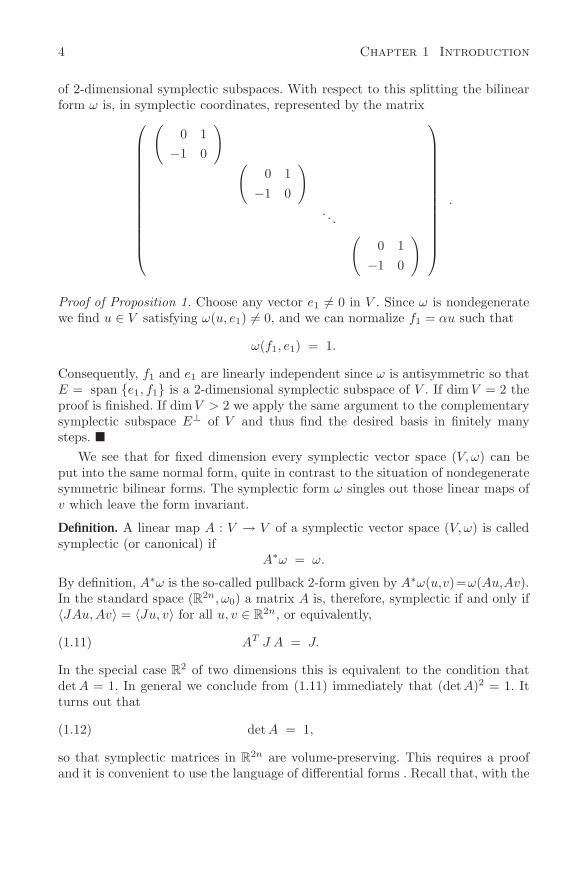
4 Chapter 1 Introduction
of 2-dimensional symplectic subspaces. With respect to this splitting the bilinearform ω is, in symplectic coordinates, represented by the matrix
(0 1
−1 0
)
(0 1
−1 0
)
. . . (0 1
−1 0
)
.
Proof of Proposition 1. Choose any vector e1 = 0 in V . Since ω is nondegeneratewe find u ∈ V satisfying ω(u, e1) = 0, and we can normalize f1 = αu such that
ω(f1, e1) = 1.
Consequently, f1 and e1 are linearly independent since ω is antisymmetric so thatE = span e1, f1 is a 2-dimensional symplectic subspace of V . If dim V = 2 theproof is finished. If dim V > 2 we apply the same argument to the complementarysymplectic subspace E⊥ of V and thus find the desired basis in finitely manysteps.
We see that for fixed dimension every symplectic vector space (V, ω) can beput into the same normal form, quite in contrast to the situation of nondegeneratesymmetric bilinear forms. The symplectic form ω singles out those linear maps ofv which leave the form invariant.
Definition. A linear map A : V → V of a symplectic vector space (V, ω) is calledsymplectic (or canonical) if
A∗ω = ω.
By definition, A∗ω is the so-called pullback 2-form given by A∗ω(u,v)=ω(Au,Av).In the standard space (R2n, ω0) a matrix A is, therefore, symplectic if and only if〈JAu,Av〉 = 〈Ju, v〉 for all u, v ∈ R
2n, or equivalently,
AT J A = J.(1.11)
In the special case R2 of two dimensions this is equivalent to the condition that
det A = 1. In general we conclude from (1.11) immediately that (detA)2 = 1. Itturns out that
det A = 1,(1.12)
so that symplectic matrices in R2n are volume-preserving. This requires a proof
and it is convenient to use the language of differential forms . Recall that, with the
1.1 Symplectic vector spaces 5
coordinates z = (z1, . . . , z2n) ∈ R2n, the bilinear form dzi ∧ dzj on R
2n is definedby
(dzi ∧ dzj)(u, v) = uivj − ujvi,
for u, v ∈ R2n. Introducing the notation z = (x, y) ∈ R
2n, we can, therefore,represent ω0 in the form
ω0 =n∑
j=1
dyj ∧ dxj .
Then the 2n-formΩ = ω0 ∧ ω0 ∧ . . . ∧ ω0 (n times )
on R2n is the volume form
Ω = c dx1 ∧ . . . ∧ dxn ∧ dy1 ∧ . . . ∧ dyn
with a constant c = 0. If A is a matrix in R2n then A∗Ω = (det A)Ω by the
definition of a determinant. Assuming that A∗ω0 = ω0 we conclude A∗Ω = Ω and,hence, det A = 1 as claimed.
The set of symplectic matrices in R2n, which meet the conditions (1.11), is
a group under matrix multiplication. It is one of the classical Lie groups and isdenoted by Sp(n).
Proposition 2. If A and B ∈ Sp(n) then A−1, AB ∈ Sp(n). Moreover, AT ∈ Sp(n)and J ∈ Sp(n).
Proof. By multiplying AT JA = J with A−1 from the right and with (AT )−1 fromthe left, we find J = (AT )−1JA−1 so that A−1 ∈ Sp(n). Taking now the inverseon both sides of the latter identity we find J−1 = AJ−1AT , and since J−1 = −J
we find (AT )TJAT = J and AT ∈ Sp(n).
Note that if a 2n by 2n matrix is written in block form
U =
(A B
C D
)(1.13)
with respect to the splitting R2n = R
n × Rn, it is symplectic if and only if
AT C , BT D are symmetric and AT D − CT B = 1,
as is readily verified. For example, a matrix U having B = 0 is symplectic if andonly if A is nonsingular and U can be written as
U =
A 0
0 (AT )−1
(1 0
S 1
),
with some symmetric matrix S.
6 Chapter 1 Introduction
Definition. If (V , ω1 1) and (V , ω2 2) are two symplectic vector spaces we call a linearmap A : V1 → V2 symplectic if
A∗ω2 = ω1,
where, by definition, (A∗ω2)(u, v) = ω2(Au,Av) for all u, v ∈ V1. Clearly A isinjective such that dim V1 ≤ dim V2.
Proposition 3. If (V1, ω1) and (V2, ω2) are two symplectic spaces of the same dimen-sion, then there exists a linear isomorphism A : V1 → V2 satisfying A∗ω2 = ω1.
This means that all symplectic vector spaces of the same dimension are, in thissense, equivalent; they are symplectically indistinguishable.
Proof. The proof follows immediately from the normal form in Proposition 1.Choosing symplectic bases (ej , fj) in (V1, ω1) and (ej , fj) in (V2, ω2) we define thelinear map A : V1 → V2 by
A ej = ej and A fj = fj
for 1 ≤ j ≤ n. Then clearly A∗ω2 = ω1 by definition of a symplectic basis. Since the choice of e1 and e1 in the construction of the symplectic bases is at our
disposal we conclude from the above proof that the group Sp(n) acts transitivelyin R
2n. Moreover, it also acts transitively on the set of symplectic subspaces of R2n
having the same dimension. This follows because a symplectic basis in a subspaceE can always be completed to a basis of V by adding a symplectic basis of itscomplement E⊥, as we did in the proof of Proposition 1.
1.2 Symplectic diffeomorphisms and Hamiltonianvector fields in (R2n, ω0)
We now turn to nonlinear maps in the symplectic space (R2n, ω0). A diffeomor-phism ϕ in R
2n is called symplectic if
ϕ∗ω0 = ω0,(1.14)
where, by definition, the pullback of any 2-form ω is given by
(ϕ∗ω)x(a, b) = ωϕ(x)(ϕ′(x)a, ϕ′(x)b)
for x ∈ R2n and for all a, b ∈ TxR
2n = R2n. Here ϕ′(x) denotes the derivative
of ϕ at the point x represented by the Jacobian matrix. In view of the definitionof ω0, a symplectic diffeomorphism in (R2n, ω0) is, therefore, characterized by theidentity
ϕ′(x)T J ϕ′(x) = J , x ∈ R2n(1.15)
1.2 Symplectic diffeomorphisms and Hamiltonian vector fields 7
for the first derivatives of ϕ. Hence ϕ′(x) is a symplectic matrix and, in particular,
detϕ′(x) = 1,(1.16)
so that symplectic diffeomorphisms are volume-preserving. However, if n > 1 theclass of symplectic diffeomorphisms is much more restricted than that of volume-preserving diffeomorphisms. This will become clear below when, taking our leadfrom Gromov, we look at the question: what can be done with symplectic diffeo-morphisms?
A symplectic diffeomorphism ϕ in (R2n, ω0) not only preserves ω0 and theassociated volume form Ω but also the action of closed curves, as we shall seenext. The form ω0 is an exact form, since
ω0 =n∑
j=1
dyj ∧ dxj = dλ,(1.17)
with the 1-form λ defined by
λ =n∑
j=1
yj dxj .
Therefore, λ−ϕ∗λ is a closed form provided ϕ is symplectic. Indeed, d(λ−ϕ∗λ) =dλ − d(ϕ∗λ) = dλ − ϕ∗dλ = ω0 − ϕ∗ω0 = 0. Using the Poincare lemma one findsa function F : R
2n → R satisfying
λ − ϕ∗λ = dF.(1.18)
If γ is an oriented simply closed curve we can integrate and find in view of (1.18)∫
γ
λ =∫
γ
ϕ∗λ =∫
ϕ(γ)
λ
since the integral of an exact form over a closed curve vanishes. Defining the actionA(γ) of a closed curve γ by
A(γ) =∫
γ
λ ∈ R,(1.19)
we see that
A(ϕ(γ)
)= A(γ)(1.20)
provided ϕ is symplectic; hence ϕ leaves the action invariant as claimed. Con-versely, of course, if a diffeomorphism ϕ in R
2n satisfies (1.20) for all closed curves
8 Chapter 1 Introduction
in R2n we conclude that ϕ is symplectic. Parameterizing γ by x(t), with 0 ≤ t ≤ 1
and x(0) = x(1), the action becomes
A(γ) =12
1∫
0
〈−Jx, x〉 dt.(1.21)
Examples of symplectic diffeomorphisms are generated by the so-called Hamilto-nian vector fields which we now recall. To the symplectic form ω0 and to a smoothfunction
H : R2n → R,
we can associate a vector field XH on R2n by requiring
ω0
(XH(x), a
)= −dH(x)a(1.22)
for all a ∈ R2n and x ∈ R
2n. Since ω0 is nondegenerate, the vector XH(x) is deter-mined uniquely. The condition (1.22) is equivalent to 〈JXH(x), a〉 = −〈∇H(x), a〉where the gradient of H is, as usual, defined with respect to the Euclidean innerproduct. Therefore, JXH(x) = −∇H(x) and in view of J2 = −1 we find therepresentation
XH(x) = J∇H(x) , x ∈ R2n.(1.23)
Clearly the Hamiltonian vector fields are very special. They differ in particularsharply from vector fields X = ∇H(x) of gradient type, since J is antisymmetric.
In the following we denote by ϕt the flow of a vector field X. It is defined by
d
dtϕt(x) = X
(ϕt(x)
)
ϕ0(x) = x , x ∈ R2n .
The curve x(t) = ϕt(x) solves the Cauchy initial value problem for the initialcondition x ∈ R
2n. Assume now that X = XH is the Hamiltonian vector fielddetermined by ω0 and H. Then every flow map ϕt preserves the form ω0:
(ϕt)∗ ω0 = ω0,(1.24)
and is, therefore, a symplectic map. This is easily verified and will be proved inthe next section in a more abstract setting.
It is useful for the following to recall the transformation formula for vectorfields X on R
m. Assume x(t) is a solution of the differential equation
x = X(x) , x ∈ Rm.
1.3 Hamiltonian vector fields and symplectic manifolds 9
If u : Rm → R
m is a diffeomorphism we can define the curve y(t) by
x(t) = u(y(t)
).
Differentiating in t we conclude that y(t) solves the equation
y = Y (y) , y ∈ Rm
for the transformed vector field Y defined by
Y (y) = du(y)−1 · X u(y).
In the following, we shall use the notation
u∗X : = (du)−1 · X u.(1.25)
We have demonstrated that the two flows ϕt of X and ψt of u∗X are conjugatedby the diffeomorphism u, i.e.,
ϕt u = u ψt .
If we subject a Hamiltonian vector field XH in R2n to an arbitrary transformation u
its special form will be destroyed. However, a symplectic transformation preservesthe class of Hamiltonian vector fields. Indeed, if u∗ω0 = ω0 then
u∗XH = XK and K = H u.(1.26)
This is easily verified: defining the function K as the composition K = H u,then by the chain rule, dK = dH u · du, and the gradient with respect to theEuclidean scalar product becomes ∇K = (du)T∇H u. By assumption, du is, atevery point, a symplectic map and, therefore, also (du)T so that du ·J · (du)T = J .Consequently, in view of the definition (1.23) of a Hamiltonian vector field
XK = J∇K = J(du)T ∇H u
= (du)−1(J∇H) u
= u∗XH ,
as we set out to prove.
1.3 Hamiltonian vector fields and symplectic manifolds
In order to introduce Hamiltonian vector fields on a manifold, we first have toextend the symplectic structure
ω0 =n∑
j=1
dyj ∧ dxj on R2n
to even dimensional manifolds.
10 Chapter 1 Introduction
Definition. A symplectic structure on an even dimensional manifold M is a 2-formω on M satisfying
(i) dω = 0, i.e., ω is a closed form.
(ii) ω is nondegenerate.
The second condition requires that for every tangent space TxM : if ωx(u, v) = 0for all v ∈ TxM then u = 0. The pair (M,ω) is then called a symplectic manifold.Thus every tangent space TxM of a symplectic manifold becomes a symplecticvector space with respect to the distinguished antisymmetric and nondegeneratebilinear form ωx at x. Therefore, M has even dimension.
An example is the symplectic manifold (R2n, ω0); indeed, since ω0 is a constantform we have dω0 = 0. Since the symplectic form ω is assumed to be closed, everysymplectic manifold looks, locally, like (R2n, ω0); we shall now prove that thereare always local coordinates in which the symplectic form is represented by theconstant form ω0.
Theorem 1. (Darboux) Suppose ω is a nondegenerate 2-form on a manifold ofdim M = 2n. Then dω = 0 if and only if at each point p ∈ M there are coordinates(U,ϕ) where ϕ : (x1, . . . , xn, y1, . . . , yn) → q ∈ U ⊂ M satisfies ϕ(0) = p and
ϕ∗ω = ω0 =n∑
j=1
dyj ∧ dxj.
Such coordinates are sometimes called symplectic coordinates. They are clearlynot determined uniquely; the most general coordinates of this sort are related to(x, y) by symplectic transformation u∗ω0 = ω0 in R
2n, as previously introduced.We see that we can define a symplectic manifold alternatively as follows: it isa manifold of dim M = 2n for which there are local coordinates ϕj mappingopen sets Uj ⊂ M onto open sets of the fixed symplectic space (R2n, ω0) suchthat the coordinates changes ϕi ϕ−1
j defined on ϕj(Ui ∩Uj) are symplectic localdiffeomorphisms in (R2n, ω0).
Proof. Choosing any local coordinates, we may assume that ω is a 2-form on R2n
depending on z ∈ R2n and that p corresponds to z = 0. By a linear change of
coordinates we can achieve that the form be in normal form at the origin, i.e.,
ω(0) =n∑
j=1
dyj ∧ dxj at z = 0.
This is precisely the same as the statement that any nondegenerate antisymmet-ric bilinear form can be brought into normal form (Proposition 1). With ω0 weshall denote the constant form Σdyj ∧ dxj on R
2n. The aim is to find a localdiffeomorphism ϕ in a neighborhood of 0 leaving the origin fixed and solving
ϕ∗ω = ω0.
1.3 Hamiltonian vector fields and symplectic manifolds 11
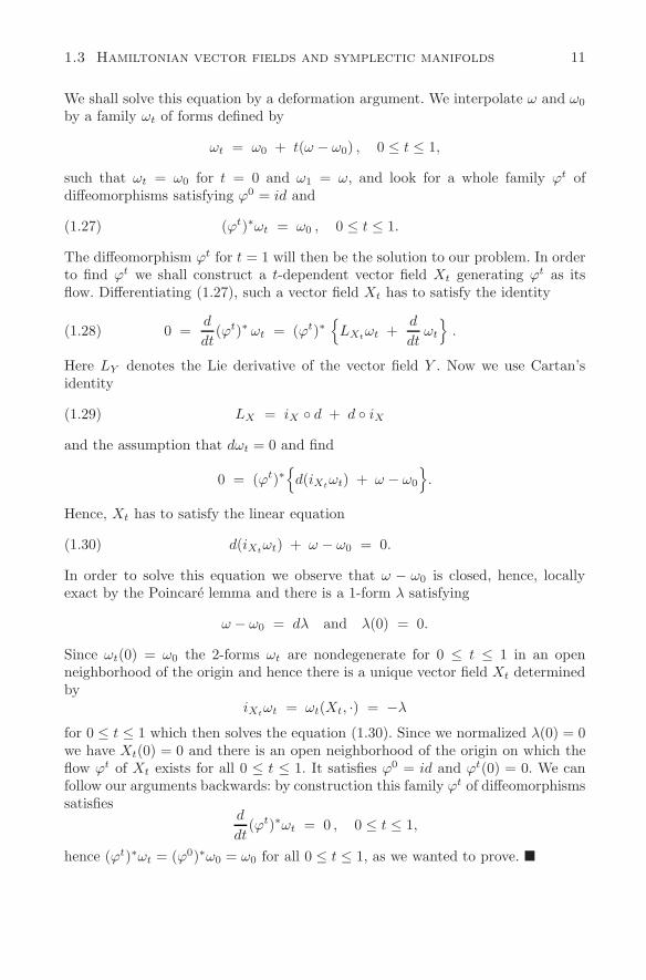
We shall solve this equation by a deformation argument. We interpolate ω and ω0
by a family ωt of forms defined by
ωt = ω0 + t(ω − ω0) , 0 ≤ t ≤ 1,
such that ωt = ω0 for t = 0 and ω1 = ω, and look for a whole family ϕt ofdiffeomorphisms satisfying ϕ0 = id and
(ϕt)∗ωt = ω0 , 0 ≤ t ≤ 1.(1.27)
The diffeomorphism ϕt for t = 1 will then be the solution to our problem. In orderto find ϕt we shall construct a t-dependent vector field Xt generating ϕt as itsflow. Differentiating (1.27), such a vector field Xt has to satisfy the identity
0 =d
dt(ϕt)∗ ωt = (ϕt)∗
LXt
ωt +d
dtωt
.(1.28)
Here LY denotes the Lie derivative of the vector field Y . Now we use Cartan’sidentity
LX = iX d + d iX(1.29)
and the assumption that dωt = 0 and find
0 = (ϕt)∗d(iXt
ωt) + ω − ω0
.
Hence, Xt has to satisfy the linear equation
d(iXtωt) + ω − ω0 = 0.(1.30)
In order to solve this equation we observe that ω − ω0 is closed, hence, locallyexact by the Poincare lemma and there is a 1-form λ satisfying
ω − ω0 = dλ and λ(0) = 0.
Since ωt(0) = ω0 the 2-forms ωt are nondegenerate for 0 ≤ t ≤ 1 in an openneighborhood of the origin and hence there is a unique vector field Xt determinedby
iXtωt = ωt(Xt, ·) = −λ
for 0 ≤ t ≤ 1 which then solves the equation (1.30). Since we normalized λ(0) = 0we have Xt(0) = 0 and there is an open neighborhood of the origin on which theflow ϕt of Xt exists for all 0 ≤ t ≤ 1. It satisfies ϕ0 = id and ϕt(0) = 0. We canfollow our arguments backwards: by construction this family ϕt of diffeomorphismssatisfies
d
dt(ϕt)∗ωt = 0 , 0 ≤ t ≤ 1,
hence (ϕt)∗ωt = (ϕ0)∗ω0 = ω0 for all 0 ≤ t ≤ 1, as we wanted to prove.
12 Chapter 1 Introduction
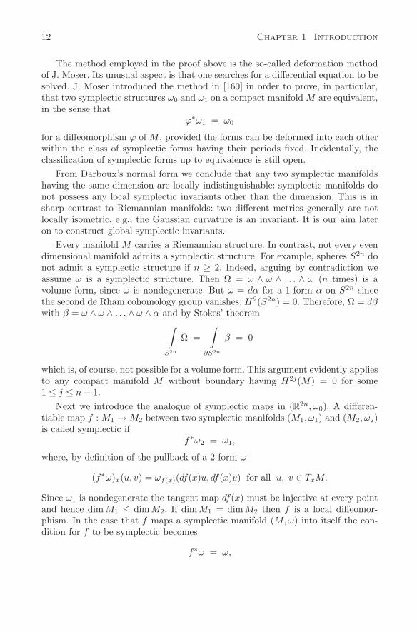
The method employed in the proof above is the so-called deformation methodof J. Moser. Its unusual aspect is that one searches for a differential equation to besolved. J. Moser introduced the method in [160] in order to prove, in particular,that two symplectic structures ω0 and ω1 on a compact manifold M are equivalent,in the sense that
ϕ∗ω1 = ω0
for a diffeomorphism ϕ of M , provided the forms can be deformed into each otherwithin the class of symplectic forms having their periods fixed. Incidentally, theclassification of symplectic forms up to equivalence is still open.
From Darboux’s normal form we conclude that any two symplectic manifoldshaving the same dimension are locally indistinguishable: symplectic manifolds donot possess any local symplectic invariants other than the dimension. This is insharp contrast to Riemannian manifolds: two different metrics generally are notlocally isometric, e.g., the Gaussian curvature is an invariant. It is our aim lateron to construct global symplectic invariants.
Every manifold M carries a Riemannian structure. In contrast, not every evendimensional manifold admits a symplectic structure. For example, spheres S2n donot admit a symplectic structure if n ≥ 2. Indeed, arguing by contradiction weassume ω is a symplectic structure. Then Ω = ω ∧ ω ∧ . . . ∧ ω (n times) is avolume form, since ω is nondegenerate. But ω = dα for a 1-form α on S2n sincethe second de Rham cohomology group vanishes: H2(S2n) = 0. Therefore, Ω = dβwith β = ω ∧ ω ∧ . . . ∧ ω ∧ α and by Stokes’ theorem
∫
S2n
Ω =∫
∂S2n
β = 0
which is, of course, not possible for a volume form. This argument evidently appliesto any compact manifold M without boundary having H2j(M) = 0 for some1 ≤ j ≤ n − 1.
Next we introduce the analogue of symplectic maps in (R2n, ω0). A differen-tiable map f : M1 → M2 between two symplectic manifolds (M1, ω1) and (M2, ω2)is called symplectic if
f∗ω2 = ω1,
where, by definition of the pullback of a 2-form ω
(f∗ω)x(u, v) = ωf(x)(df(x)u, df(x)v) for all u, v ∈ TxM.
Since ω1 is nondegenerate the tangent map df(x) must be injective at every pointand hence dim M1 ≤ dim M2. If dim M1 = dim M2 then f is a local diffeomor-phism. In the case that f maps a symplectic manifold (M,ω) into itself the con-dition for f to be symplectic becomes
f∗ω = ω,
1.3 Hamiltonian vector fields and symplectic manifolds 13
i.e., f preserves the symplectic structure. Expressed in the distinguished localsymplectic coordinates defined by Darboux’s theorem, this condition for f agreeswith our previous condition for a map to be symplectic in (R2n, ω0). It is useful topoint out that locally such a symplectic map can be presented in terms of a singlefunction on R
2n, a so-called generating function and we refer to the Appendix fordetails.
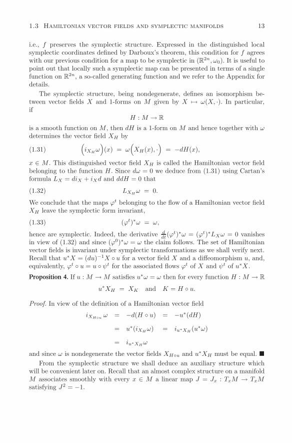
The symplectic structure, being nondegenerate, defines an isomorphism be-tween vector fields X and 1-forms on M given by X → ω(X, ·). In particular,if
H : M → R
is a smooth function on M , then dH is a 1-form on M and hence together with ωdetermines the vector field XH by(
iXHω)(x) = ω
(XH(x), ·
)= −dH(x),(1.31)
x ∈ M . This distinguished vector field XH is called the Hamiltonian vector fieldbelonging to the function H. Since dω = 0 we deduce from (1.31) using Cartan’sformula LX = diX + iXd and ddH = 0 that
LXHω = 0.(1.32)
We conclude that the maps ϕt belonging to the flow of a Hamiltonian vector fieldXH leave the symplectic form invariant,
(ϕt)∗ω = ω,(1.33)
hence are symplectic. Indeed, the derivative ddt(ϕ
t)∗ω = (ϕt)∗LXω = 0 vanishesin view of (1.32) and since (ϕ0)∗ω = ω the claim follows. The set of Hamiltonianvector fields is invariant under symplectic transformations as we shall verify next.Recall that u∗X = (du)−1X u for a vector field X and a diffeomorphism u, and,equivalently, ϕt u = u ψt for the associated flows ϕt of X and ψt of u∗X.
Proposition 4. If u : M → M satisfies u∗ω = ω then for every function H : M → R
u∗XH = XK and K = H u.
Proof. In view of the definition of a Hamiltonian vector field
iXHuω = −d(H u) = −u∗(dH)
= u∗(iXHω) = iu∗XH
(u∗ω)
= iu∗XHω
and since ω is nondegenerate the vector fields XHu and u∗XH must be equal. From the symplectic structure we shall deduce an auxiliary structure which
will be convenient later on. Recall that an almost complex structure on a manifoldM associates smoothly with every x ∈ M a linear map J = Jx : TxM → TxMsatisfying J2 = −1.
14 Chapter 1 Introduction
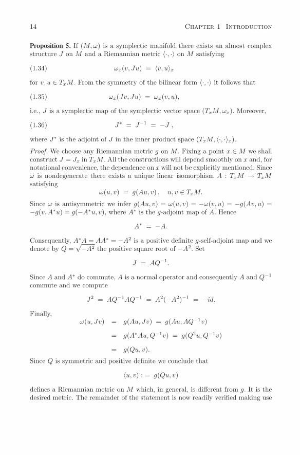
Proposition 5. If (M,ω) is a symplectic manifold there exists an almost complexstructure J on M and a Riemannian metric 〈·, ·〉 on M satisfying
ωx(v, Ju) = 〈v, u〉x(1.34)
for v, u ∈ TxM . From the symmetry of the bilinear form 〈·, ·〉 it follows that
ωx(Jv, Ju) = ωx(v, u),(1.35)
i.e., J is a symplectic map of the symplectic vector space (TxM,ωx). Moreover,
J∗ = J−1 = −J ,(1.36)
where J∗ is the adjoint of J in the inner product space (TxM, 〈·, ·〉x).
Proof. We choose any Riemannian metric g on M . Fixing a point x ∈ M we shallconstruct J = Jx in TxM . All the constructions will depend smoothly on x and, fornotational convenience, the dependence on x will not be explicitly mentioned. Sinceω is nondegenerate there exists a unique linear isomorphism A : TxM → TxMsatisfying
ω(u, v) = g(Au, v) , u, v ∈ TxM.
Since ω is antisymmetric we infer g(Au, v) = ω(u, v) = −ω(v, u) = −g(Av, u) =−g(v,A∗u) = g(−A∗u, v), where A∗ is the g-adjoint map of A. Hence
A∗ = −A.
Consequently, A∗A = AA∗ = −A2 is a positive definite g-self-adjoint map and wedenote by Q =
√−A2 the positive square root of −A2. Set
J = AQ−1.
Since A and A∗ do commute, A is a normal operator and consequently A and Q−1
commute and we compute
J2 = AQ−1AQ−1 = A2(−A2)−1 = −id.
Finally,ω(u, Jv) = g(Au, Jv) = g(Au,AQ−1v)
= g(A∗Au,Q−1v) = g(Q2u,Q−1v)
= g(Qu, v).
Since Q is symmetric and positive definite we conclude that
〈u, v〉 : = g(Qu, v)
defines a Riemannian metric on M which, in general, is different from g. It is thedesired metric. The remainder of the statement is now readily verified making use
1.3 Hamiltonian vector fields and symplectic manifolds 15
of the fact that the metric 〈u, v〉 = 〈v, u〉 is symmetric. Since the constructiondepends smoothly on x the proof is completed.
This almost complex structure compatible with ω extends the complex struc-ture in (R2n, ω0) considered above. Moreover, if ∇H denotes the gradient of afunction H with respect to the Riemannian metric 〈·, ·〉 of Proposition 5, i.e.,〈∇H(x), v〉 = dH(x)v for all v ∈ TxM , we find for the Hamiltonian vector fieldXH the representation
XH(x) = J∇H(x) ∈ TxM(1.37)
using that J2 = −1. This agrees with the representation of XH in (R2n, ω0).We should point out that the almost complex structure is not unique. If we
denote by Jω the set of almost complex structures compatible with ω in the senseof (1.34), it can easily be shown that this set is contractible. Indeed, for everyJ ∈ Jω there exists, by definition, a unique Riemannian metric gJ satisfyingω(u, Jv) = gJ(u, v). Starting from any Riemannian metric g, we constructed inthe proof of the proposition an almost complex structure J = Jg and a metric gJ
such that JgJ= J . Hence, fixing any metric g∗ on M , we can define the contraction
in Jω by(t, J) → J(1−t)gJ+tg∗
for 0 ≤ t ≤ 1 and J ∈ Jω.In view of Darboux’s theorem there are locally no symplectic invariants other
than the dimension. On the other hand, the total volume is a trivial example ofa global symplectic invariant. Indeed, if u : (M1, ω1) → (M2, ω2) is a symplecticdiffeomorphism of M1 onto M2 then it follows from u∗ω2 = ω1 that the associatedvolume forms Ω1 = ω1 ∧ . . . ∧ ω1 (n times) on M1 and similarly Ω2 on M2 arerelated by
u∗Ω2 = Ω1.(1.38)
Since the diffeomorphism u : M1 → M2 preserves the orientation we have∫
M1
u∗Ω2 =∫
M2
Ω2
and in view of (1.38), ∫
M1
Ω1 =∫
M2
Ω2,
so that the total volumes of Ω1 and Ω2 have to agree. Consider now the special caseof compact, connected and oriented manifolds of dimension 2, i.e., surfaces. Theorientation will be given by a volume form denoted by ω. It evidently is a closedform, since every 3-form on a surface vanishes. Therefore, (M,ω) is a symplecticmanifold with the volume form as the symplectic structure.
16 Chapter 1 Introduction
Assume now that (M1, ω1) and (M2, ω2) are two such surfaces and let u : M1 →M2 be a symplectic diffeomorphism u∗ω2 = ω1, which in dimension 2 is the sameas a volume-preserving diffeomorphism, then
∫
M1
ω1 =∫
M2
ω2,(1.39)
so that the volumes agree. Our aim is to prove the converse. We shall prove that iftwo compact, connected and oriented surfaces (M1, ω1) and (M2, ω2) are diffeomor-phic (which is the case if their Euler characteristics are equal) and if, in addition,their total volumes agree, then there exists a diffeomorphism u : M1 → M2, whichsatisfies u∗ω2 = ω1. This gives a classification of compact connected 2-dimensionalsymplectic manifolds according to the Euler characteristic and the total volume.More generally we shall prove the following statement for volume preserving dif-feomorphisms.
Theorem 2. (Moser) Assume M is a compact, connected and oriented manifold ofdimension m without boundary. If α and β are two volume forms such that theirtotal volumes agree, i.e.,
∫
M
α =∫
M
β,(1.40)
then there is a diffeomorphism u of M satisfying u∗β = α.
Consequently the total volume is the only invariant of volume-preserving dif-feomorphisms.
Proof. We proceed as in the proof of Darboux’s theorem and deform the volumeform α into β defining
αt = (1 − t)α + tβ , 0 ≤ t ≤ 1.
These forms αt are volume forms since locally α and β are represented by α =a(x)dx1∧. . .∧dxm and β = b(x)dx1∧. . .∧dxm with nonvanishing smooth functionsa and b, which, by assumption (1.40), must have the same sign. We shall constructa family ϕt of diffeomorphisms satisfying
(ϕt
)∗αt = α , ϕ0 = id(1.41)
for 0 ≤ t ≤ 1, so that the diffeomorphism u = ϕ1 will solve our problem. Since Mis compact, connected and oriented we conclude from
∫M
(β − α) = 0 that
β − α = dγ(1.42)
1.3 Hamiltonian vector fields and symplectic manifolds 17
for some (m − 1)-form γ on M . This is a special case of the de Rham theorem.Since αt is a volume form we find a unique time-dependent vector field Xt on Msolving the linear equation
iXtαt = −γ
for 0 ≤ t ≤ 1. Denote by ϕt the flow of this vector field Xt satisfying ϕ0 = id.Since M is compact it exists for all t. Since dαt = 0 for volume forms we find,again using Cartan’s formula,
ddt
(ϕt
)∗αt =
(ϕt
)∗(LXt
αt + ddt
αt
)
=(ϕt
)∗(d(iXt
αt) + β − α),
which vanishes since d(iXtαt) + β − α = d(iXt
αt + γ) = 0 by our choice of thevector field Xt. Therefore (1.41) holds and the proof is finished.
We have seen that symplectic diffeomorphisms are volume-preserving diffeo-morphisms so that the total volume is a (trivial) global symplectic invariant. More-over, for volume-preserving diffeomorphisms, this is the only invariant. One of ouraims later on is to establish symplectic invariants other than the volume whichwill prove that symplectic diffeomorphisms are of a different nature than volume-preserving diffeomorphisms. An example of such a global symplectic invariant isprompted by Darboux’s theorem. Recall that this theorem states that locally nearevery point on a symplectic manifold (M,ω) there is a local diffeomorphism ϕfrom a small ball of R
2n into M satisfying ϕ∗ω = ω0. This means in particularthat there is always a symplectic embedding of a small open ball B(r) into M ,
ϕ :(B(r), ω0
)→ (M,ω),
where B(r) = x ∈ R2n | |x|2 < r2.
We should mention that this is, of course, only a local result; even on R2n with
n ≥ 2 there exist symplectic structures ω of infinite volume for which there isno diffeomorphism ϕ of R
2n solving ϕ∗ω = ω0. The existence of such an exoticsymplectic structure is a deep result due to M. Gromov [107].
We now look for the largest ball B(r) ⊂ R2n which can be symplectically
embedded into a given symplectic manifold (M,ω) of dimension dimM = 2n, anddefine
D(M,ω) = sup
πr2∣∣∣ there existsa symplectic embedding ϕ :
(B(r), ω0
)→ (M,ω)
.
This is a positive number or ∞ which we shall call the Gromov width of (M,ω).At this point we cannot explain why we choose πr2 in the definition and not,for example, the volume of B(r). We mention, however, that πr2 agrees withthe action |A(γ)| for every closed characteristic γ on the boundary ∂B(r) of thestandard sphere of radius r in R
2n. This will be explained later on.

18 Chapter 1 Introduction
It is easy to see that D(M,ω) is a symplectic invariant. We first show thatD(M,ω) has a monotonicity property in the sense that
D(M,ω) ≤ D(N, τ),(1.43)
if there exists a symplectic embedding ψ : M → N . To every symplectic embeddingϕ : B(r) → M there is a symplectic embedding B(r) → N defined by ψ ϕ.Therefore, the supremum in the definition of D(N, τ) is taken over a possiblylarger set so that indeed D(N, τ) ≥ D(M,ω) as claimed. If f : M → N is asymplectic diffeomorphism of M onto N we can apply the monotonicity propertyto f and also to f−1 and conclude:
Proposition 6. If (M,ω) and (N, τ) are symplectically isomorphic, then D(M,ω) =D(N, τ).
We see that the Gromov width is a symplectic invariant. It will turn out, andthis is not obvious, that this invariant is quite different form the total volumeif n ≥ 2. The Gromov width is merely one example in the class of symplecticinvariants called symplectic capacities which will be introduced in Chapter 2.
1.4 Periodic orbits on energy surfaces
The existence problem we shall briefly describe originates in the search for periodicsolutions in celestial mechanics and is, as we shall see in Chapter 4, related tospecial symplectic invariants. For simplicity we consider the standard symplecticmanifold (R2n, ω0). We have seen that a function H : R
2n → R together with ω0
determines the Hamiltonian vector field XH on R2n by
iXHω0 = −dH.(1.44)
The flow ϕt of the vector field XH leaves the function H invariant, i.e.,
H(ϕt(x)
)= H(x) , x ∈ R
2n(1.45)
for all t for which the flow is defined, hence H is an integral of XH . Indeed differ-entiating (1.45) we find, using the definition of the flow
ddt
H(ϕt) = dH(ϕt) · ddt
ϕt = dH(ϕt) · XH(ϕt)
= −ω0
(XH , XH
) (ϕt) ,
which vanishes since ω0 is antisymmetric. Geometrically, the level sets
S =
x ∈ R2n
∣∣∣H(x) = const⊂ R
2n
1.4 Periodic orbits on energy surfaces 19
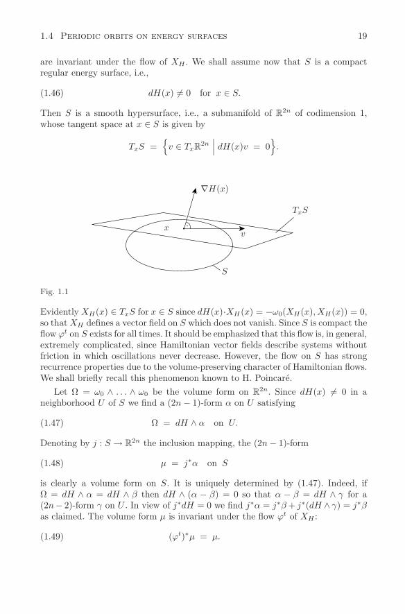
are invariant under the flow of XH . We shall assume now that S is a compactregular energy surface, i.e.,
dH(x) = 0 for x ∈ S.(1.46)
Then S is a smooth hypersurface, i.e., a submanifold of R2n of codimension 1,
whose tangent space at x ∈ S is given by
TxS =
v ∈ TxR2n
∣∣∣ dH(x)v = 0
.
∇H(x)
TxS
S
vx
Fig. 1.1
Evidently XH(x) ∈ TxS for x ∈ S since dH(x)·XH (x) = −ω0(XH(x), XH(x)) = 0,so that XH defines a vector field on S which does not vanish. Since S is compact theflow ϕt on S exists for all times. It should be emphasized that this flow is, in general,extremely complicated, since Hamiltonian vector fields describe systems withoutfriction in which oscillations never decrease. However, the flow on S has strongrecurrence properties due to the volume-preserving character of Hamiltonian flows.We shall briefly recall this phenomenon known to H. Poincare.
Let Ω = ω0 ∧ . . . ∧ ω0 be the volume form on R2n. Since dH(x) = 0 in a
neighborhood U of S we find a (2n − 1)-form α on U satisfying
Ω = dH ∧ α on U.(1.47)
Denoting by j : S → R2n the inclusion mapping, the (2n − 1)-form
µ = j∗α on S(1.48)
is clearly a volume form on S. It is uniquely determined by (1.47). Indeed, ifΩ = dH ∧ α = dH ∧ β then dH ∧ (α − β) = 0 so that α − β = dH ∧ γ for a(2n− 2)-form γ on U . In view of j∗dH = 0 we find j∗α = j∗β + j∗(dH ∧ γ) = j∗βas claimed. The volume form µ is invariant under the flow ϕt of XH :
(ϕt)∗µ = µ.(1.49)
20 Chapter 1 Introduction
This follows from (ϕt)∗Ω = Ω and (ϕt)∗dH = dH. Indeed, in view of (1.47) we firstfind Ω = dH ∧ (ϕt)∗α, and using the uniqueness we conclude j∗(ϕt)∗α = j∗α.But ϕt j = j ϕt and hence (ϕt)∗(j∗α) = (j∗α), proving the claim (1.49). If wedenote the regular measure on S associated to the form µ by m we see that
m(ϕt(A)
)= m(A) , A ⊂ S.(1.50)
Moreover, m(S) < ∞ since S is compact.
Theorem 3. (Poincare’s recurrence theorem) Let S be a compact and regular energysurface of the Hamiltonian vector field XH with flow ϕt. Then almost every point(with respect to m) on S is a recurrent point, i.e., for almost every x ∈ S there isa sequence tj ↑ ∞ satisfying
limj→∞
ϕtj (x) = x.
Proof. The proof is surprisingly easy. By ϕ we denote the time-1 map of the flowϕt. We first use the invariance and finiteness of the measure to show that for everyA ⊂ S
m(A ∩
[ ⋂k≥0
⋃j≥k
ϕ−j(A)])
= m(A).(1.51)
Observe that the points x in the above set [ · ] are those points x ∈ S which havethe property that for every integer k there is an integer j ≥ k such that x ∈ ϕ−j(A)i.e., ϕj(x) ∈ A. The intersection with A consists of the points x in A which returninfinitely often to the set A. In order to prove (1.51) we abbreviate
Ak :=⋃j≥k
ϕ−j(A) , k = 0, 1, 2, . . .
and have the decreasing sequence of subsets A0 ⊃ A1 ⊃ A2 ⊃ . . . . Clearly,ϕk(Ak) = A0 and consequently m(Ak) = m(A0) since ϕ preserves the measure.Since m(A0) < ∞ we conclude that A0 = Ak almost everywhere for k = 0, 1, 2, . . .and consequently,
⋂k≥0
Ak = A0 almost everywhere. Hence, in view of A ⊂ A0 we
findA ∩
⋂k≥0
Ak = A ∩ A0 = A almost everywhere,
which is the desired equation (1.51). Now we use the topological fact that there isa countable basis in S. For every n there are countably many open balls Bj( 1
n) of
radius 1n covering S. Applying the first step to every ball, we find a null set N ⊂ S
having the property that every x ∈ S\N returns infinitely often to every ball towhich it belongs. Since for every n there exists a j = j(x) such that x ∈ Bj( 1
n ),the theorem is proved.
1.4 Periodic orbits on energy surfaces 21
We note that the compactness is not relevant: the statement follows if theinvariant measure on S is finite and the topology of S has a countable basis.This observation allowed Poincare to apply his theorem to the restricted 3-bodyproblem.
In view of the recurrence theorem it seems quite natural to search for periodicphenomena on S. One could hope that by perturbing the Hamiltonian systemslightly some of the recurrent points do not only return infinitely often but closeup in finite time, thus giving rise to a periodic orbit. This is the so-called ClosingProblem. In their celebrated Closing-Lemma, C.C. Pugh and C. Robinson ([179]1983) proved that generically (in the C2-category of the Hamiltonian functions) theperiodic orbits are dense on a compact and regular energy surface. In sharp contrastto this generic phenomenon we are interested in the following global existencequestion:
Question. Does a compact and regular energy surface S in (R2n, ω0) possess aperiodic solution of the Hamiltonian vector field XH?
The question is still open. It should be emphasized that we are looking forperiodic solutions of a very restricted class of vector fields on S and recall that H.Seifert ([193], 1950) raised the question, whether every nonvanishing vector fieldon the three sphere S3 has a closed orbit. The problem remained open for manyyears. In 1974, P.A. Schweitzer [192] constructed a surprising vector field in theclass C1 on S3 which has no periodic solutions, and only very recently in 1993K. Kuperberg [132] gave an example of a C∞ vector field on S3 with no periodicsolutions. For manifolds with dimension higher than three the question had beenanswered similarly in 1966 by F.W. Wilson [228]. One could ask whether thereare vector fields in the more restricted class of measure-preserving smooth vectorfields not admitting any periodic solution. For the special class of Reeb vectorfields, however, the existence of closed orbits has been established quite recentlyby H. Hofer [118]: every smooth Reeb vector field on S3 possesses a periodic orbit.A vector field X on S3 is called a Reeb vector field, if there exists a 1-form λ onS3 with λ ∧ dλ defining a volume form and satisfying
iXdλ = 0 and iXλ = 1 .
We shall come back to Reeb vector fields in Chapter 4 in connection with theWeinstein conjecture on contact manifolds.
It will be crucial later on that the above question is independent of the par-ticular choice of the Hamiltonian function representing S. It only depends on thehypersurface and the symplectic structure. This fact is well-known from the regu-larization of collision singularities in the celestial 2-body problem. Assume that Fis a second function defining S, such that
S =
x∣∣∣ H(x) = c
=
x∣∣∣ F (x) = c′
(1.52)
22 Chapter 1 Introduction
with dH = 0 and dF = 0 on S. Then ker dF (x) = ker dH(x) and, therefore,dF (x) = ρ(x)dH(x) for every x ∈ S, with a nowhere-vanishing smooth functionρ. Consequently, the Hamiltonian vector fields are parallel:
XF = ρXH on S ,(1.53)
with ρ(x) = 0. It follows that XH and XF have the same orbits on S althoughtheir parametrization will be different, in general. To be more precise, if ϕt is theflow of XH on S, then the flow ψs of XF on S is given by
ψs(x) = ϕt(x) , t = t(s, x) , x ∈ S ,(1.54)
where the function t is defined by the differential equation
dt
ds= ρ
(ϕt(x)
), t(0, x) = 0 ,
depending on the parameter x ∈ S. We see that, in particular, XH has the sameperiodic orbits as XF .
For example, if XH has the energy surface S = x ∈ R2n | 1
2 |x|2 = R > 0, thenall the solutions of XH on S are periodic. Indeed, also the Hamiltonian F definedby F (x) = 1
2 |x|2 represents S = x |F (x) = R as a regular energy surface. Thevector field XF is linear and has the flow
ψs(x) = esJx = (cos s)x + (sin s)Jx,
which evidently is periodic.We can reformulate the problem more abstractly in terms of a distinguished
line bundle. Assume S is a hypersurface in R2n. Then TxS has dimension 2n − 1
so that the restriction of ω0 onto TxS must be degenerate and of rank (2n − 2).Its kernel is, therefore, 1-dimensional and we see that ω0 and S determine the linebundle
LS =(x, ξ) ∈ TS
∣∣∣ ω0(ξ, v) = 0 for all v ∈ TxS
.(1.55)
If S is a regular energy surface for XH , then ω0(XH(x), v) = −dH(x)v = 0 for allv ∈ TxS. Therefore,
XH(x) ∈ LS(x) , x ∈ S
for every Hamiltonian vector field having S as a regular energy surface. Conse-quently, the periodic solutions for XH on S correspond to the closed character-istics of the line bundle LS. These are defined as the 1-dimensional submanifoldP ⊂ S diffeomorphic to circles for which the tangent spaces belong to LS, i.e.,TP = LS|P . Therefore, the existence question of periodic solutions of Hamilto-nian equations on regular energy surfaces can be reformulated geometrically asfollows:
1.5 Existence of a periodic orbit on a convex energy surface 23
Question. Does a compact smooth hypersurface S ⊂ (R2n, ω0) admit a closedcharacteristic of the distinguished line bundle LS?
Note that LS is defined by the hypersurface and ω0. It will be demonstrated inChapter 4 that there are hypersurfaces S ⊂ R
2n and symplectic structures ω nearS and different from ω0, such that the line bundle of S with respect to ω does notadmit closed characteristics.
The breakthrough in this global existence question is due to A. Weinstein[225] and P. Rabinowitz [225] in 1978 who established the existence of a closedcharacteristic on a convex respectively star-like hypersurface in R
2n. The proofs arebased on variational principles. In particular P. Rabinowitz demonstrated that thehighly degenerate action principle previously used to derive formal transformationproperties for Hamiltonian vector fields can be used very effectively for existenceproofs. This crucial idea turned out to be decisive in the further development inwhich the next landmark was C. Viterbo’s proof of the A. Weinstein conjecture inR
2n in 1987. The conjecture states that every hypersurface of contact type carriesa closed characteristic. This type of symplectically restricted hypersurfaces will bedescribed in Chapter 4, which is devoted to the existence of closed characteristicson hypersurfaces in symplectic manifolds. We should mention that every compacthypersurface S gives rise to an abundance of periodic orbits which, however, arenot necessarily on the given surface but on surfaces nearby. We illustrate this witha result which also will be proved in Chapter 4. Assume the hypersurface S belongsto a family defined by
Sε =
x∣∣∣ H(x) = 1 + ε
⊂ R
2n
for ε in an interval I around 0, where S corresponds to S0.
Theorem 4. For almost every ε ∈ I, the hypersurface Sε in R2n possesses a periodic
solution for XH .
In Chapter 4 we shall easily deduce this phenomenon from a distinguishedsymplectic invariant.
1.5 Existence of a periodic orbit on a convex energy surface
In this section we shall prove a very special qualitative existence result, whichhistorically marked the beginning of a rapid development in global questions ofsymplectic geometry and Hamiltonian mechanics. Our purpose is to illustrate theclassical technique of direct methods of the calculus of variations. This techniqueis in sharp contrast to the more recent technique introduced in Chapter 3. InChapter 4 the result itself will be an immediate consequence of the existence of aspecial symplectic invariant.
24 Chapter 1 Introduction
Theorem 5. Assume the hypersurface S ⊂ (R2n, ω0) is the smooth (in the classC2) boundary of a compact and strictly convex region in R
2n. Then S carries aclosed orbit.
We conclude, in particular, that every Hamiltonian vector field XH having Sas a regular energy surface possesses a periodic solution on S. The result is due toP. Rabinowitz [180] and A. Weinstein [225], 1978. The proof we shall give belowis based on an idea due to F. Clarke [53].
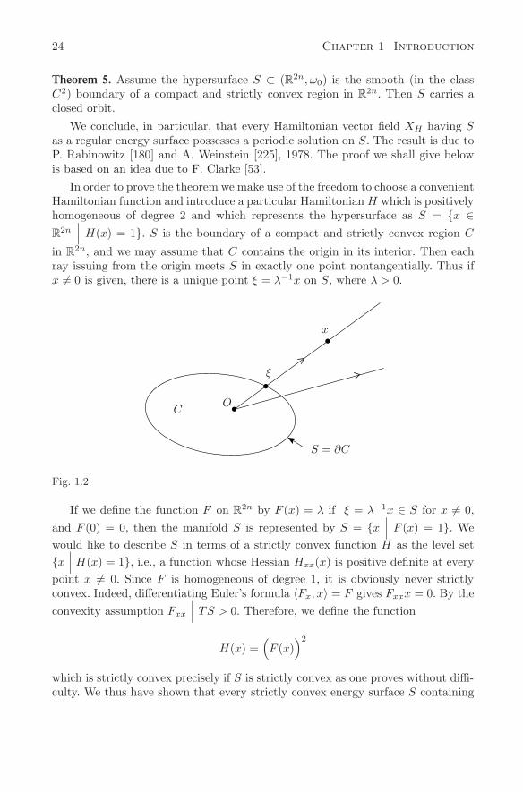
In order to prove the theorem we make use of the freedom to choose a convenientHamiltonian function and introduce a particular Hamiltonian H which is positivelyhomogeneous of degree 2 and which represents the hypersurface as S = x ∈R
2n∣∣∣ H(x) = 1. S is the boundary of a compact and strictly convex region C
in R2n, and we may assume that C contains the origin in its interior. Then each
ray issuing from the origin meets S in exactly one point nontangentially. Thus ifx = 0 is given, there is a unique point ξ = λ−1x on S, where λ > 0.
x
ξ
OC
S = ∂C
Fig. 1.2
If we define the function F on R2n by F (x) = λ if ξ = λ−1x ∈ S for x = 0,
and F (0) = 0, then the manifold S is represented by S = x∣∣∣ F (x) = 1. We
would like to describe S in terms of a strictly convex function H as the level setx
∣∣∣ H(x) = 1, i.e., a function whose Hessian Hxx(x) is positive definite at everypoint x = 0. Since F is homogeneous of degree 1, it is obviously never strictlyconvex. Indeed, differentiating Euler’s formula 〈Fx, x〉 = F gives Fxxx = 0. By theconvexity assumption Fxx
∣∣∣ TS > 0. Therefore, we define the function
H(x) =(F (x)
)2
which is strictly convex precisely if S is strictly convex as one proves without diffi-culty. We thus have shown that every strictly convex energy surface S containing
1.5 Existence of a periodic orbit on a convex energy surface 25
the origin in its interior can be represented by
S = x∣∣∣ H(x) = 1(1.56)
with a function H : R2n −→ R satisfying
(i) H ∈ C2(R2n\0), H(0) = 0
(ii) Hxx(x) > 0 if x = 0
(iii) H(ρx) = ρ2H(x) if ρ ≥ 0.
(1.57)
In view of our discussion in the previous section, it suffices to show that thisspecial Hamiltonian vector field XH possesses a periodic solution on this energysurface S, i.e., we have to show that there is a periodic solution of
x = J∇H(x) on S.
Normalizing the period we can ask for a periodic solution of period 2π on S forthe equation
x = λ J∇H(x) for some λ = 0.(1.58)
For example, the variational principle
min
2π∫
0
H(x(t)
)dt under
12
2π∫
0
〈Jx, x〉 = 1 ,
where the functions x(t) are assumed to be 2π-periodic, has the above equations asEuler equations. But one easily shows that neither the infimum nor the supremumis taken on, even if H(x) = 1
2|x|2. The trick now is to use an alternative variational
principle having the same differential equations for which, however, the infimum istaken on. We shall form the Legendre transformation of H, but in contrast to theusual Legendre transformation of physics, all variables will be transformed. Thefunction G(y) related to H(x) by a Legendre transformation can be defined by
G(y) = maxξ∈R2n
(〈ξ, y〉 − H(ξ)
)= 〈x, y〉 − H(x).
There is indeed a unique maximum x ∈ R2n given by y = ∇H(x), since Hxx(y) is
positive definite for y = 0 and since H satisfies
1c|y|2 ≤ H(y) ≤ c |y|2, y ∈ R
2n(1.59)
for some constant c > 1. The estimate is an immediate consequence of the homo-geneity of H. Summarizing, we have
G(y) + H(x) = 〈x, y〉(1.60)
26 Chapter 1 Introduction
fory = ∇H(x) and x = ∇G(y).(1.61)
Clearly G(0) = 0, G ∈ C2(R2n\0) and G is positively homogeneous of degree2. Since Hxx(x) · Gyy(y) = 1l for x = 0, G is also strictly convex if y = 0, so thatG enjoys the same properties as H :
(i) G(0) = 0, G ∈ C2(R2n\0)
(ii) Gyy(y) > 0 if y = 0
(iii) G(ρy) = ρ2G(y) for ρ ≥ 0.
We now look at the new, alternate, variational principle for 2π-periodic functions z:
min
2π∫
0
G(z)dt under12
2π∫
0
〈Jz, z〉 = 1 ,(1.62)
which we shall solve by the standard direct variational methods. To be more pre-cise, we define the following function space F of periodic functions z(t) = z(t+2π)having mean value 0:
F = z ∈ H1(S1)∣∣∣ 1
2π
2π∫
0
z(t)dt = 0 ,
where H1(S1) is the Hilbert space of absolutely continuous 2π-periodic functionswhose derivatives are square integrable, i.e., belong to L2(S1). Note that with zalso z+ const. is a solution of (1.62), hence the condition on the mean value fixesthe constant. By A ⊂ F we shall denote the subset
A = z ∈ F∣∣∣ 1
2
2π∫
0
〈Jz, z〉 = 1.
Following the standard procedure we shall verify that the functional
I(z) =
2π∫
0
G(z(t)
)dt on A
meets the following properties:
(i) It is bounded from below on A.
1.5 Existence of a periodic orbit on a convex energy surface 27
(ii) It takes on its minimum on A, i.e., there exists z∗ ∈ A satisfying2π∫0
G(z∗)dt = infz∈A
2π∫0
G(z)dt = µ > 0.
(iii) z∗ solves the Euler equations
∇G(z∗) = αJz∗ + β
in L2(S1) with constants α = 0 and β.
(iv) z∗ belongs to C2 and satisfies
z∗ = ∇H(αJz∗ + β)
pointwise, and x(t) = c (αJz∗(t)+β) is the desired solution of x = J∇H(x)on S for an appropriate constant c.
Ad (i): We need some estimates. Since every z belonging to F has mean valuezero, the Poincare inequality
‖z‖ ≤ ‖z‖ , z ∈ F
holds, where ‖·‖ denotes the L2 norm. This follows simply from the Fourier series.For z ∈ A we conclude
2 =
2π∫
0
〈Jz, z〉 ≤ ‖z‖ ‖z‖ ≤ ‖z‖2, z ∈ A.(1.63)
The function G being strictly convex and positively homogeneous of degree 2satisfies the estimate 1
K|y|2 ≤ G(y) ≤ K|y|2 for y ∈ R
2n with some constantK ≥ 1. Therefore, by means of (1.63), we find for z ∈ A
2π∫
0
G(z)dt ≥ 1K
‖z‖2 ≥ 2K
> 0 ,(1.64)
i.e., the functional is bounded from below by a positive constant, in particular,µ > 0.Ad (ii): We choose a minimizing sequence zj ∈ A such that
limj→∞
2π∫
0
G(zj)dt = µ.(1.65)
In view of (1.63) and (1.64) there is a constant M > 0 with 2 ≤ ‖zj‖2 ≤ Mand we obtain ‖zj‖ ≥ 2‖zj‖−1 ≥ 2√
Mand hence, by Poincare’s inequality 2√
M≤
28 Chapter 1 Introduction
‖zj‖ ≤√
M . In particular zj is a bounded sequence in the Hilbert space H1(S1)and, therefore, a subsequence, also denoted by zj converges weakly in H1(S1) toan element z∗ ∈ H1(S1) :
zj → z∗ weakly in H1(S1).(1.66)
We have used the well-known fact that the closed unit ball of a Hilbert space isweakly sequentially compact. In addition, for a function z∗ ∈ C(S1) ,
supt
|zj(t) − z∗(t)| → 0 ,(1.67)
i.e., zj converges uniformly to z∗. Indeed the zj are equicontinuous:
|zj(t) − zj(τ)| ≤ |t∫
τ
zj(s)ds |
≤ |t − τ |1/2‖zj‖≤ |t − τ |1/2
√M,
and the claim follows from the Arzela-Ascoli theorem. Clearly z∗(t) = z∗(t) almosteverywhere. Indeed, with the L2 inner product we can write (z∗ − z∗, z∗ − z∗) =(zj−z∗, z∗−z∗)+(z∗−zj , z∗−z∗). The first term on the right hand side convergesto 0 in view of the uniform convergence and the second one in view of the weakconvergence.
We shall show that z∗ ∈ A. By (1.67) we conclude that the mean value of z∗vanishes. Also,
2 =
2π∫
0
〈Jzj , zj〉 =
2π∫
0
〈J(zj − z∗), zj〉 +
2π∫
0
〈Jz∗, zj〉.
The first term on the right hand side tends to 0 by (1.67) since ‖zj‖ ≤√
M isbounded, and the second term converges by (1.66) so that
2π∫
0
〈Jz∗, z∗〉 = 2
and therefore z∗ ∈ A. We next show that this z∗ is a minimum. From the convexityof G we deduce the pointwise estimate 〈∇G(y1), y2 − y1 〉 ≤ G(y2) − G(y1) ≤〈∇G(y2), y2 − y1〉, which applied to z∗(t) = y2 and y1 = zj(t) gives
2π∫
0
G(z∗)dt −2π∫
0
G(zj)dt ≤2π∫
0
〈∇G(z∗), z∗ − zj〉dt.
1.5 Existence of a periodic orbit on a convex energy surface 29
Observing that ∇G, being positively homogeneous of degree 1, satisfies an estimate|∇G(y)| ≤ C|y| for y ∈ R
2n and for some constant C > 0, we conclude that ∇G(z∗)belongs to L2 so that the right hand side tends to zero, since (z∗− zj) → 0 weaklyin L2. Thus
µ ≤2π∫
0
G(z∗) ≤ lim infj→∞
2π∫
0
G(zj)dt = µ
by (1.65) and we have proved that z∗ is a minimum of I(z), for z ∈ A.
Ad (iii): Since z∗ is a minimum, we have
2π∫
0
〈∇G(z∗), ζ〉 = 0(1.68)
for every test function ζ ∈ F satisfying
2π∫
0
〈Jz∗, ζ〉 = 0.(1.69)
We now choose ζ of the form
ζ = ∇G(z∗) − αJz∗ − β
with two constants α und β. In order that ζ be periodic we pick β so that themean value of ζ is zero:
2π∫
0
ζdt =
2π∫
0
∇G(z∗)dt − 2πβ = 0 ,
and next determine the constant α so that (1.69) holds true. Using again that z∗has mean value zero we find that the equation
0 =
2π∫
0
〈Jz∗, ζ〉 =
2π∫
0
〈Jz∗ , ∇G(z∗)〉 − α
2π∫
0
〈Jz∗, Jz∗〉(1.70)
has a unique solution α, since its coefficient does not vanish. With this test functionζ we compute
2π∫
0
|ζ|2 =
2π∫
0
〈∇G(z∗), ζ〉 − α
2π∫
0
〈Jz∗, ζ〉 − 〈β,
2π∫
0
ζ〉
30 Chapter 1 Introduction
which, in view of the condition (1.68) vanishes. We conclude that z∗ satisfies theEuler equations
∇G(z∗) = αJz∗ + β(1.71)
for constants α and β, as was, of course, to be expected. For the constant α wefind α = µ, so that α > 0. Indeed, using the Euler equations and the homogeneityof G we compute
2µ = 2
2π∫
0
G(z∗) =
2π∫
0
〈∇G(z∗), z∗〉 = α
2π∫
0
〈Jz∗, z∗〉 = 2α .
Ad (iv): It is easy to see that z∗ belongs to C2. Recalling that x = ∇G(y) isinverted by y = ∇H(x) pointwise we find from the Euler equations that
z∗(t) = ∇H(αJz∗(t) + β)(1.72)
for almost every t. The right hand side is continuous and we conclude that z∗ ∈ C1,and, inserting it again into the right hand side, we find z∗ ∈ C2. Finally, setting
x(t) = c(αJz∗(t) + β
),
with c > 0, we obtain from (1.72) using the homogeneity of ∇H
x = c αJ ∇H(αJz∗ + β) = αJ ∇H(x)
and, since H is of degree 2,
2π∫
0
H(x)dt =12
2π∫
0
〈∇H(x), x〉 =12c2α
2π∫
0
〈z∗, Jz∗〉 = c2α
which is equal to 2π if we choose c =√
2πα . Therefore, x(t) is a 2π-periodic solution
of the equation x = αJ ∇H(x) and lies on the energy surface H = 1. Consequentlyy(t) = x(α−1t) is the desired periodic solution of x = J∇H(x) on H = 1 whichhas the period T = 2πα = 2πµ. But this is unimportant since the period of theperiodic solution on S depends on our choice of the Hamiltonian function. Thisfinishes the proof of the theorem.
Recalling the transformation properties of Hamiltonian vector fields, one con-cludes from the above theorem that every hypersurface in R
2n which is symplec-tically diffeomorphic to a strictly convex one, always possesses a closed charac-teristic. Such a situation is, however, hard to recognize and we shall see belowthat there are hypersurfaces which are not symplectically diffeomorphic to convexones. It will be our aim in Chapter 4 to describe symplectically invariant prop-erties of a hypersurface which guarantee the existence of a closed characteristic.
1.6 The problem of symplectic embeddings 31
The existence will, however, be established by means of a very different variationalprinciple.
The idea of the above proof, sometimes called the dual action principle, prompt-ed many existence results for convex Hamiltonians. For example, I. Ekeland [65]1984 established a Morse theory for periodic solutions on convex hypersurfaceswhich is analogous to the one for closed geodesics on compact Riemannian man-ifolds. Using Ekeland’s Morse theory he showed that generically (in the C∞ cat-egory) every compact and convex hypersurface S ⊂ R
2n carries infinitely manyperiodic orbits [65, 66, 67]. In the special case that the convex surface S ⊂ R
2n isclose to a round sphere in the sense that
B(r) ⊂ S ⊂ B(R) and R ≤√
2r
for two open balls of radius r and R (where the first inclusion means contained inthe inside of S), one can prove that S carries at least n closed characteristics [70].Here the convexity requirement can be relaxed somewhat and we refer to [21] forthe precise statement.
For an account of this circle of questions concerning convex Hamiltonians,we refer to the recent book by I. Ekeland: “Convexity Methods in HamiltonianMechanics” (1990), [66].
1.6 The problem of symplectic embeddings
We consider two compact connected domains D1 and D2 in Rm having smooth
boundaries. If the domains are diffeomorphic by an orientation preserving diffeo-morphism, one can ask the question: under what additional conditions on D1 andD2 does there exist a volume-preserving diffeomorphism, i.e., a diffeomorphismϕ : D1 → D2 satisfying det ϕ′(x) = 1 for every x in the interior of D1? Clearly,
vol (D1) = vol (D2)
is a necessary condition. It turns out that this is already the only condition which isalso sufficient for the existence of a volume-preserving diffeomorphism. This followsfrom the following extension of Theorem 2 in Section 3 to the case of manifoldswith boundaries.
Theorem 6. (Dacorogna-Moser) Let D1 and D2 be two compact connected domainswith smooth boundaries in R
m. Assume α(x) = a(x) dx1 ∧ . . . ∧ dxm is a smoothvolume form on D1 and β(x) = b(x)dx1∧ . . .∧dxm is a smooth volume form on D2
with a > 0 and b > 0. If ϕ : D1 → D2 is an orientation preserving diffeomorphism,then there exists a diffeomorphism ψ : D1 → D2 satisfying, in addition, ψ = ϕ on∂D1 and
det(ψ′(x)
)· b
(ψ(x)
)= λa(x),
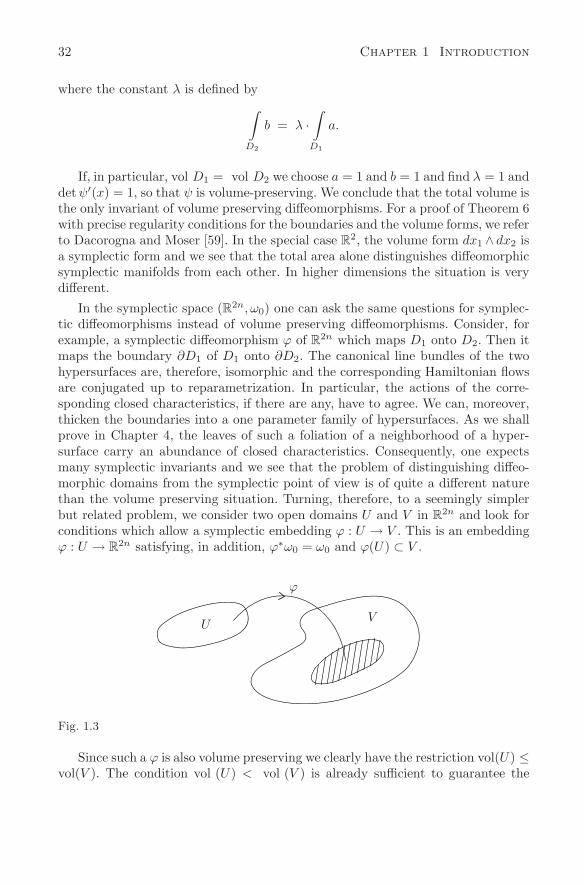
32 Chapter 1 Introduction
where the constant λ is defined by∫
D2
b = λ ·∫
D1
a.
If, in particular, vol D1 = vol D2 we choose a = 1 and b = 1 and find λ = 1 anddet ψ′(x) = 1, so that ψ is volume-preserving. We conclude that the total volume isthe only invariant of volume preserving diffeomorphisms. For a proof of Theorem 6with precise regularity conditions for the boundaries and the volume forms, we referto Dacorogna and Moser [59]. In the special case R
2, the volume form dx1 ∧ dx2 isa symplectic form and we see that the total area alone distinguishes diffeomorphicsymplectic manifolds from each other. In higher dimensions the situation is verydifferent.
In the symplectic space (R2n, ω0) one can ask the same questions for symplec-tic diffeomorphisms instead of volume preserving diffeomorphisms. Consider, forexample, a symplectic diffeomorphism ϕ of R
2n which maps D1 onto D2. Then itmaps the boundary ∂D1 of D1 onto ∂D2. The canonical line bundles of the twohypersurfaces are, therefore, isomorphic and the corresponding Hamiltonian flowsare conjugated up to reparametrization. In particular, the actions of the corre-sponding closed characteristics, if there are any, have to agree. We can, moreover,thicken the boundaries into a one parameter family of hypersurfaces. As we shallprove in Chapter 4, the leaves of such a foliation of a neighborhood of a hyper-surface carry an abundance of closed characteristics. Consequently, one expectsmany symplectic invariants and we see that the problem of distinguishing diffeo-morphic domains from the symplectic point of view is of quite a different naturethan the volume preserving situation. Turning, therefore, to a seemingly simplerbut related problem, we consider two open domains U and V in R
2n and look forconditions which allow a symplectic embedding ϕ : U → V . This is an embeddingϕ : U → R
2n satisfying, in addition, ϕ∗ω0 = ω0 and ϕ(U) ⊂ V .
U
ϕ
V
Fig. 1.3
Since such a ϕ is also volume preserving we clearly have the restriction vol(U) ≤vol(V ). The condition vol (U) < vol (V ) is already sufficient to guarantee the
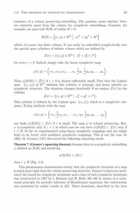
1.6 The problem of symplectic embeddings 33
existence of a volume preserving embedding. The question arises whether thereare obstacles apart from the volume for symplectic embeddings. Consider, forexample, an open ball B(R) of radius R > 0:
B(R) =
(x, y) ∈ R2n
∣∣∣ |x|2 + |y|2 < R2
which, of course, has finite volume. It can easily be embedded symplectically intothe special open cylinders of infinite volume which are defined by
Z(r) =(x, y) ∈ R
2n∣∣ x2
1 + x22 < r2
for every r > 0. Indeed, simply take the linear symplectic map
ϕ(x, y) =(
εx1, εx2, x3, . . . , xn,1εy1,
1εy2, y3, . . . , yn
).
Then ϕ(B(R)) ⊂ Z(r) if ε > 0 is chosen sufficiently small. Note that the 2-planespan e1, e2 of R
2n defining this cylinder is isotropic and hence inherits nosymplectic structure. The situation changes drastically if we replace Z(r) by thecylinder
Z(r) =(x, y) ∈ R
2n∣∣ x2
1 + y21 < r2
.
This cylinder is defined by the 2-plane span e1, f1 which is a symplectic sub-space. Trying similarly with the map
ψ(x, y) =(
εx1,1εx2, x3, . . . , xn, εy1,
1εy2, y3, . . . , yn
)
one finds ψ(B(R)) ⊂ Z(r) if ε is small. The map ψ is volume preserving. But,ψ is symplectic only if ε = 1 in which case we can have ψ(B(R)) ⊂ Z(r) only ifr ≥ R. So far we experimented using linear symplectic mappings and one mighthope to do better with nonlinear symplectic mappings. This is not the case. In1985, M. Gromov [107] discovered the following surprising result.
Theorem 7. (Gromov’s squeezing theorem) Assume there is a symplectic embeddingϕ defined on B(R) and satisfying
ϕ(B(R)) ⊂ Z(r)
then r ≥ R (Fig. 1.4).This phenomenon demonstrates clearly that the symplectic structure of a map
is much more rigid than the volume preserving structure. Gromov’s discovery moti-vated the search for symplectic invariants and a class of such symplectic invariantswas constructed in 1987 by I. Ekeland and H. Hofer [68, 69] by means of a varia-tional principle for periodic solutions of Hamiltonian equations; the constructionwas motivated by earlier results in [67]. These invariants, described in the next
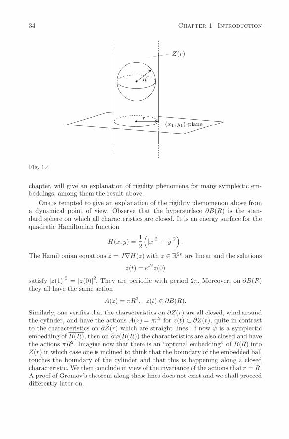
34 Chapter 1 Introduction
R
r
Z(r)
(x1, y1)-plane
Fig. 1.4
chapter, will give an explanation of rigidity phenomena for many symplectic em-beddings, among them the result above.
One is tempted to give an explanation of the rigidity phenomenon above froma dynamical point of view. Observe that the hypersurface ∂B(R) is the stan-dard sphere on which all characteristics are closed. It is an energy surface for thequadratic Hamiltonian function
H(x, y) =12
(|x|2 + |y|2
).
The Hamiltonian equations z = J∇H(z) with z ∈ R2n are linear and the solutions
z(t) = eJtz(0)
satisfy |z(1)|2 = |z(0)|2. They are periodic with period 2π. Moreover, on ∂B(R)they all have the same action
A(z) = πR2, z(t) ∈ ∂B(R).
Similarly, one verifies that the characteristics on ∂Z(r) are all closed, wind aroundthe cylinder, and have the actions A(z) = πr2 for z(t) ⊂ ∂Z(r), quite in contrastto the characteristics on ∂Z(r) which are straight lines. If now ϕ is a symplecticembedding of B(R), then on ∂ϕ(B(R)) the characteristics are also closed and havethe actions πR2. Imagine now that there is an “optimal embedding” of B(R) intoZ(r) in which case one is inclined to think that the boundary of the embedded balltouches the boundary of the cylinder and that this is happening along a closedcharacteristic. We then conclude in view of the invariance of the actions that r = R.A proof of Gromov’s theorem along these lines does not exist and we shall proceeddifferently later on.
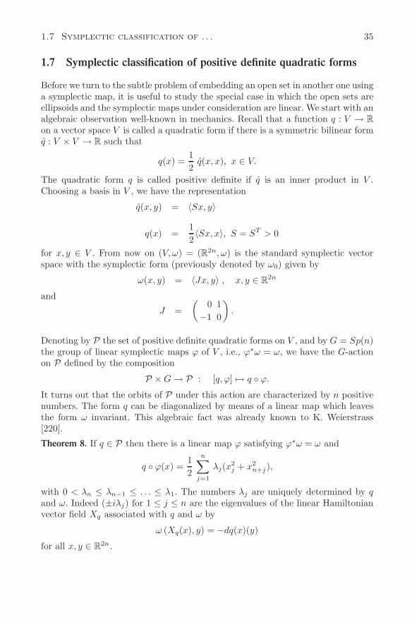
1.7 Symplectic classification of . . . 35
1.7 Symplectic classification of positive definite quadratic forms
Before we turn to the subtle problem of embedding an open set in another one usinga symplectic map, it is useful to study the special case in which the open sets areellipsoids and the symplectic maps under consideration are linear. We start with analgebraic observation well-known in mechanics. Recall that a function q : V → R
on a vector space V is called a quadratic form if there is a symmetric bilinear formq : V × V → R such that
q(x) =12
q(x, x), x ∈ V.
The quadratic form q is called positive definite if q is an inner product in V .Choosing a basis in V , we have the representation
q(x, y) = 〈Sx, y〉
q(x) =12〈Sx, x〉, S = ST > 0
for x, y ∈ V . From now on (V, ω) = (R2n, ω) is the standard symplectic vectorspace with the symplectic form (previously denoted by ω0) given by
ω(x, y) = 〈Jx, y〉 , x, y ∈ R2n
and
J =(
0−1
10
).
Denoting by P the set of positive definite quadratic forms on V , and by G = Sp(n)the group of linear symplectic maps ϕ of V , i.e., ϕ∗ω = ω, we have the G-actionon P defined by the composition
P × G → P : [q, ϕ] → q ϕ.
It turns out that the orbits of P under this action are characterized by n positivenumbers. The form q can be diagonalized by means of a linear map which leavesthe form ω invariant. This algebraic fact was already known to K. Weierstrass[220].
Theorem 8. If q ∈ P then there is a linear map ϕ satisfying ϕ∗ω = ω and
q ϕ(x) =12
n∑j=1
λj(x2j + x2
n+j),
with 0 < λn ≤ λn−1 ≤ . . . ≤ λ1. The numbers λj are uniquely determined by qand ω. Indeed (±iλj) for 1 ≤ j ≤ n are the eigenvalues of the linear Hamiltonianvector field Xq associated with q and ω by
ω (Xq(x), y) = −dq(x)(y)
for all x, y ∈ R2n.
36 Chapter 1 Introduction
Postponing the proof we observe that if q(x) = 12〈Sx, x〉 with a positive def-
inite symmetric matrix S, then Xq is the linear vector field Xq(x) = JSx, andif τ ∈ Sp(n) is any symplectic matrix, we conclude by the transformation law ofHamiltonian vector fields
Xqτ = τ−1 · Xq · τ.
Thus the two linear vector fields Xq and Xqτ are similar to each other and have,therefore, the same eigenvalues. Associating with q the n positive real numbersλ = λ(q) ∈ R
n guaranteed by the theorem, we conclude that
λ(q τ) = λ(q)
for all q ∈ P and τ ∈ Sp(n), so that these numbers characterize the orbits of Punder Sp(n).
This is, of course, in contrast to the action of the orthogonal group of ma-trices satisfying AT A = 1. Since q A(x) = 1
2 〈SAx,Ax〉 = 12〈AT SAx, x〉 =
12〈A−1SAx, x〉 we see that the orbits of P under O(2n) are determined by the
2n positive eigenvalues of the symmetric matrix S in contrast to the n imagi-nary eigenvalue pairs (±iλj) of JS. On R
2, for example, a positive quadratic formis, after an orthogonal transformation, of the form q(x) = 1
2 〈Sx, x〉 with a di-agonal matrix S = Diag (λ1, λ2) and λj > 0. The theorem guarantees a linearmap τ satisfying det τ = 1 which transforms q into the symplectic normal formq τ(x) = 1
2〈Qx, x〉 with Q = Diag (λ, λ). Geometrically the ellipsoid q(x) < 1is symplectically mapped onto the disc q τ(x) < 1 having the same area. Wesee that in R
2 the normal forms correspond to discs distinguished by the area.
Proof. On the product space (x, y) ∈ V ×V , the functions K(x, y) = q(x)+q(y) andω(x, y) are quadratic forms. Since K is positive definite we can apply a well-knownvariational argument. On the compact manifold M = M(q) defined by
M = (x, y) ∈ V × V | q(x) + q(y) = 1 ,
the continuous function (x, y) → ω(x, y) attains a maximum, say at (a, b) ∈ M ,such that
ω(a, b) = max ω(x, y).(x, y) ∈ M
We point out that a critical point (a, b) ∈ M of ω|M lies in a whole circle consistingof critical points belonging to the same critical level. Indeed, if we define the circleaction on V × V by
eit · (x, y) = (x(t), y(t)) , t ∈ R,
wherex(t) = (cos t)x + (sin t)y, y(t) = (cos t)y − (sin t)x,
1.7 Symplectic classification of . . . 37
then one verifies readily that the quadratic forms are invariant under the action,i.e.,
K (x(t), y(t)) = K (x, y) and ω (x(t), y(t)) = ω (x, y)
for all (x, y) ∈ V × V .
If λ ∈ R denotes the Lagrange multiplier of the critical point (a, b) ∈ V × V ,we have for the derivatives dK(a, b) = λ dω(a, b) or explicitly
q(a, x) = dq(a)(x) = λ ω(x, b)(1.73)
q(y, b) = dq(b)(y) = λ ω(a, y)
for every x, y ∈ V . We have used the representation dq(x)(y) = q(x, y) of thederivative of q. In view of q(x) = 1
2 q(x, x) one concludes from (1.73) that 2 =2(q(a) + q(b)) = 2λ ω(a, b). Since the maximum ω(a, b) is positive,
ω(a, b) =1λ
> 0.(1.74)
In particular, a, b are linearly independent in V since ω is antisymmetric. Asω(a, b) = 0 the 2-dimensional subspace V1 = span a, b ⊂ V is symplectic. It isthe eigenspace of Xq belonging to the pair ±iλ of purely imaginary eigenvalues.Indeed, the equations (1.73) are equivalent to
Xq(a) = +λb and Xq(b) = −λa
so that Xq(a ± ib) = ∓(iλ)(a ± ib). Normalizing, we introduce e1 = αa, f1 = −αbwith α2 = λ and find ω(f1, e1) = 1. Hence the pair e1, f1 constitutes a symplecticbasis of V1 for which
q(e1) = q(f1) =λ
2and q(e1, f1) = 0.(1.75)
Recalling the identity q(x, y) = q(x + y) − q(x) − q(y) for x, y ∈ V , we, therefore,have
q(v) =λ
2(ξ2 + η2)(1.76)
if v = ξe1 + ηf1 ∈ V1, which is the desired normal form in V1. In order to iteratethis argument we denote by
V ⊥1 = v ∈ V | ω(v1, v) = 0 for all v1 ∈ V1
the symplectic complement in V . Then V ⊥1 is a symplectic subspace and
V = V1 ⊕ V ⊥1 .
38 Chapter 1 Introduction
Indeed, V1 ∩ V ⊥1 = 0 since ω is nondegenerate on V1; moreover v − ω(v, e1)f1 +
ω(v, f1)e1 ∈ V ⊥1 for every v ∈ V so that V = V1 +V ⊥
1 . If v ∈ V1 and w ∈ V ⊥1 then
ω(v, w) = 0 and we claim that v and w are also orthogonal with respect to q:
q(v, w) = 0.
This is true, since V1 is an eigenspace. Indeed, by inserting x and y ∈ V ⊥1 into the
equations (1.73), the right hand side vanishes, hence also the left hand side, andsince V1 = span a, b, the claim is proved. Equivalently we have
q(v + w) = q(v) + q(w) if v ∈ V1 and w ∈ V ⊥1 .(1.77)
We can apply the same arguments as above to the restriction of q onto the sym-plectic space V ⊥
1 . Iteratively we find a splitting V = V1 ⊕ V2 ⊕ · · · ⊕ Vn into ndistinguished 2-dimensional symplectic spaces Vj , which are the eigenspaces of Xq
belonging to the pairs (∓iλj) of eigenvalues, with λj > 0. In view of (1.77)
q(v) = q(v1) + q(v2) + · · · + q(vn)
if v = v1 +v2 + · · ·+vn with vj ∈ Vj . Moreover, there are symplectic bases (ej , fj)in Vj such that
q(v) =12
n∑j=1
λj(x2j + x2
n+j)
if v =n∑
j=1
(xjej + xn+jfj). This is the required normal form of q and the proof of
Theorem 8 is finished. Changing the notation and introducing λi = 2
r2i
, i = 1, 2, . . . , n, we shall writefor the normal form
q ϕ(x) =n∑
j=1
1r2j
(x2j + x2
j+n),
hence associating with every q ∈ P, the positive numbers
0 < r1(q) ≤ r2(q) ≤ · · · ≤ rn(q)
which characterize the orbits of the Sp(n)-action on P. Abbreviating r = (r1, r2,. . ., rn) we have proved:
Proposition 7.r(q) = r(q ϕ)
for all q ∈ P and all ϕ ∈ Sp(n). Moreover, if
r(q) = r(Q)
for q,Q ∈ P then there is a ϕ ∈ Sp(n) satisfying Q = q ϕ.
1.7 Symplectic classification of . . . 39
Proposition 8. Assume q and Q ∈ P.
Q ≤ q =⇒ rj(q) ≤ rj(Q) for 1 ≤ j ≤ n.
Proof. From our proof of Theorem 8 we know, recalling the notation above,
12rn(q)2 =
1λn(q)
= maxM(q)
ω = ω(a, b) ,
where M(q) = (x, y) ∈ V × V | q(x) + q(y) = 1. Since Q(x) ≤ q(x) for allx ∈ V there exists α ≥ 1 such that 1 = Q(αa) + Q(αb). Hence (αa, αb) ∈ M(Q) =(x, y)|Q(x) + Q(y) = 1 and ω(αa, αb) = α2 ω(a, b) ≥ ω(a, b). Taking themaximum of ω on M(Q), we conclude rn(Q) ≥ rn(q). More generally, one verifiesthe estimates rj(Q) ≥ rj(q) for 1 ≤ j ≤ n readily, using the following minimaxcharacterization of the critical levels:
12rj(q)2 = min
W∈Fj
max
W∩M(q)ω
,
where Fj denotes the family of all linear subspaces W ⊂ V × V of dimension2n + 2j and 1 ≤ j ≤ n. Indeed, recalling that ω and K are, on the productspace V × V , quadratic forms and that K is positive definite, this is simply theCourant-Hilbert minimax principle for the eigenvalues of the symmetric matrixassociated to the form ω with respect to the inner product defined by the positiveform K. We took, however, into account that the problem is invariant under thecircle action defined above. In particular, if (a, b) ∈ V × V is a critical point then(−b, a) is also a critical point on the same critical level. Hence each eigenvalue inthe Courant-Hilbert principle has multiplicity at least 2. The general principle willgive the positive characteristic levels c4n ≥ c4n−1 · · · ≥ c2n+1, and, in order to findall the positive critical levels, we have chosen above
12rj(q)2 = c2n+2j
for 1 ≤ j ≤ n. In order to interpret the above results geometrically, we associate with the form
q ∈ P the ellipsoid E(q), defined as the open set
E(q) = x | q(x) < 1 ⊂ R2n.(1.78)
The group action of Sp(n) is then visualized by
ϕ−1(E(q)) = E(q ϕ).(1.79)
Observe that
E(q) ⊂ E(Q) ⇐⇒ q ≥ Q ,(1.80)
40 Chapter 1 Introduction
so that E(q) = E(Q) if and only if q = Q. We can, therefore, associate with theopen set E, the numbers r(E), defined by
r(E) = r(q) if E = E(q).(1.81)
In view of (1.79), we conclude from Proposition 7 that the numbers r are invariantunder the group of linear symplectic mappings. Summarizing, we have proved:
Proposition 9. If E,F are ellipsoids and ϕ ∈ Sp(n) then
r (ϕ(E)) = r(E).
Conversely, if r(E) = r(F ) then there exists a map ϕ ∈ Sp(n) satisfying ϕ(E) =F .
The crucial observation now is that these invariants have a monotonicity prop-erty. Indeed, in view of (1.80) the Proposition 8 can be restated as follows.
Proposition 10. If E, F are ellipsoids, then
E ⊂ F ⇒ rj(E) ≤ rj(F ) for 1 ≤ j ≤ n .
Conversely, if rj(E) ≤ rj(F ) for 1 ≤ j ≤ n, then there exists a ϕ ∈ Sp(n) satisfyingϕ(E) ⊂ F .
Summarizing our considerations, we have defined for the open sets E of ellip-soids in R
2n the invariants r(E) which allow us to answer the question of linearsymplectic embeddings of ellipsoids as follows:
Theorem 9. If E and F are two ellipsoids, then there exists ϕ ∈ Sp(n) such that
ϕ(E) ⊂ F
if and only if rj(E) ≤ rj(F ) for all 1 ≤ j ≤ n. We illustrate the statement with an example. If B = B(R) = x| |x|2 < R2
is the open ball of radius R, then rj(B) = R for all 1 ≤ j ≤ n and we can finda map ϕ ∈ Sp(n) embedding B into the ellipsoid E if and only if E is restrictedby the condition r1(E) ≥ R. All this is, of course, not surprising. After all weconsider only linear symplectic mappings and one might hope that the use ofnonlinear symplectic embeddings is more flexible. It turns out, however, and thisis a very surprising phenomenon discovered only recently, that if ϕ : B(R) → Eis any symplectic embedding then, r1(E) ≥ R still. We shall prove this rigiditystatement later on using a global symplectic invariant c(U) defined for every openset U ⊂ R
2n and satisfying c(ϕ(U)) = c(U) for symplectic diffeomorphisms. Thisinvariant extends r1 so that c(E) = πr1(E)2 for ellipsoids E. It has, in addition,the monotonicity property in the sense that c(U) ≤ c(V ) provided there is asymplectic embedding ϕ : U → V .
Since the construction of this global invariant c will be related to special pe-riodic solutions of Hamiltonian equations, it is useful to interpret the symplectic
1.7 Symplectic classification of . . . 41
invariants r(E) from a dynamical point of view. There is a relation between r(E)and certain closed characteristics on the boundary ∂E of E, which is the compacthypersurface
∂E = z | q(z) = 1 , if E = E(q).
We may assume q to be in normal form
q(z) =n∑
j=1
x2j + y2
j
r2j
.
Correspondingly, V splits into the 2-dimensional symplectic planes V = V1 ⊕V2 ⊕· · ·⊕Vn and zj = (xj , yj) ∈ R
2 are the symplectic coordinates in Vj . The solutionsz(t) = (z1(t), . . . , zn(t)) of the associated Hamiltonian vector field Xq are easilycomputed. Setting λj = 2
r2j
, we have
zj(t) = etλjJzj(0), 1 ≤ j ≤ n,
where J is the standard 2 × 2 matrix of the symplectic structure. Consequently,∂E∩Vj carries the distinguished periodic solution wj(t) = (0, . . . , 0, zj(t), 0, . . . , 0)given by
zj(t) = etλjJzj(0) and |zj(0)|2 = r2j
and having period T = πr2j . Its action, a global symplectic invariant, is
A(wj) =12
T∫
0
〈−Jwj , wj〉 = πr2j .
We see that the invariant rj of the set E is represented by a closed characteristicon ∂E. In particular,
πr1(E)2 = min |A(z)| : z is a closed characteristic on ∂E .
In the following, the dynamical approach will be extremely useful in the con-struction of symplectic invariants.
We would like to add that the quadratic forms play an important role if onestudies the orbit structure of a Hamiltonian vector field XH locally near an equi-librium point, i.e., a point at which XH vanishes. We shall finish this chapter bydescribing some well-known results illustrating this. We may assume the equilib-rium to be the origin, so that ∇H(0) = 0 and
XH(z) = JHzz(0)z + · · ·
for z near the origin in R2n. From now on we shall assume the eigenvalues of
JHzz(0) to be purely imaginary, so that (±iλj) for 1 ≤ j ≤ n are all the eigenval-ues. If one assumes, in addition, that JHzz(0) can be diagonalized symplectically
42 Chapter 1 Introduction
one can write, after a linear symplectic transformation,
H(z) =12
n∑j=1
λj(x2j + y2
j ) + · · · ,
with real numbers λj ∈ R. In view of Theorem 8, we can always achieve this nor-mal form if Hzz(0) is positive definite. Now R
2n is decomposed into the sum ofsymplectic 2-planes (xj , yj) which are filled with periodic solutions of the linearsystem z = JHzz(0)z having periods 2π
|λj| . The question arises whether these fami-lies have a continuation to solutions of the nonlinear system near z = 0. The vectorfield XH may not admit any periodic solution except z = 0, as examples show.By restricting the λj , a well-known result due to Lyapunov [145] guarantees acontinuation under infinitely many nonresonance conditions. It is, therefore, quiteremarkable that in the positive definite case studied above, no such conditions areneeded, as the following result due to A. Weinstein [223] demonstrates:
Theorem 10. Assume Hzz(0) > 0. Then there are at least n closed characteristics onthe hypersurfaces H(z)−H(0) = ε2 for ε > 0 sufficiently small. As parameterizedsolutions of the system XH , they have periods close to the ones of the linearizedsystem z = JHzz(0)z.
This local existence statement has been generalized by J. Moser [163]. Theperiodic solutions mentioned so far are prompted by the solutions of the linearizedequation and we turn now to genuinely nonlinear phenomena. First we recall anonlinear normal form of H at z = 0 which goes back to G. Birkhoff ([26] 1927),and which establishes nonlinear local symplectic invariants associated with H atthe equilibrium point.
1.8 The orbit structure near an equilibrium, Birkhoff normal form
If H is a smooth function of the form
H(z) =n∑
j=1
αj
2(x2
j + y2j ) + . . . = H2 + . . .
near the equilibrium point z = 0, then we consider the group action H τ where τbelongs to the group G1 of symplectic and smooth diffeomorphisms defined locallynear z = 0 and leaving the origin and the quadratic part H2 of H invariant,
G1 = τ∣∣∣ τ∗ω0 = ω0 and τ(0) = 0, dτ(0) = id.
The aim is to find a map τ ∈ G1 such that Hτ is in a particularly simple form. Weemphasize that, in the following, the quadratic part H2 is fixed and not assumedto be a definite quadratic form.
1.8 The orbit structure near an equilibrium . . . 43
Theorem 11. (Birkhoff normal form) Assume the linear invariants α = (α1, α2,. . ., αn) are nonresonant of order s, i.e.,
〈α, j〉 = 0 for j ∈ Zn, 0 < |j| ≤ s,
where |j| =n∑
ν=1
|jν |. Then there exists an analytic map τ ∈ G1 such that
H τ = F (I1, . . . , In) + os,
where F is a polynomial of degree [ s2 ] in the n variables I = (I1, I2, . . . , In) of
the formF = 〈α, I〉 +
12〈βI, I〉 + . . . ,
with a n × n matrix β. The functions Ij on R2n are given by
Ij (x, y) =12
(x2j + y2
j ) for 1 ≤ j ≤ n .
In addition, the polynomial F is uniquely determined by H and does not dependon the choice of τ ∈ G1.
The coefficients of F are, therefore, local symplectic invariants of H called theBirkhoff invariants. Postponing the discussion about the significance of this normalform, we first give the proof, which is of an algebraic nature.
Proof. We proceed iteratively and assume that
H = H2 + H3 + . . . + Hm−1 + Hm + . . .
is already in normal form up to order m−1, where Hj are homogeneous polynomialsof degree j. We look for a symplectic map τ ∈ G1 which does not change the normalform already achieved and which puts H τ into normal form up to order m. Wetake
τ = exp XP ,
i.e., the time-1 map of the Hamiltonian vector field XP , with a homogeneouspolynomial P of degree m. Since τ belongs to the flow of a Hamiltonian vectorfield it is symplectic, and of the form
τ(z) = z + J∇P (z) + . . . ,
where the dots stand for the higher order terms, and one computes readily
H τ = H2 + H3 + . . . + Hm−1 + (Hm − H2, P) + . . . .
The polynomial in the parenthesis is homogeneous of degree m and the bracket·, · stands for the Poisson bracket defined for two functions F and G as follows:
F, G = ω(XG, XF ).
We see that we can modify H by functions of the form H2, P.Denote by Vm the vector space of homogeneous polynomials of degree m and
let L : Vm −→ Vm be the linear operator defined by L(P ) = H2, P for P ∈ Vm.
44 Chapter 1 Introduction
Lemma 1. The kernel K = K(L) and the range R = R(L) of the linear operatorL are complementary:
Vm = K + R and K ∩ R = 0 .
If, in addition, 〈α, j〉 = 0 for 0 < |j| ≤ m, then K = 0 if m is odd. If m = 2k iseven, then
K = span Ik11 . . . Ikn
n
∣∣∣n∑
j=1
kj = k .
The normal form, therefore, consists of elements in the kernel of L, and weshall abbreviate the set of normal forms by
N = P∣∣∣ H2, P = 0 and P is a polynomial .
Proof of the Lemma. In order to diagonalize L in Vm, we go to complex variablesand choose the symplectic coordinates
ξν = 1√2
(xν + iyν)ην = 1√
2(yν + ixν)
so that ξvην = i2 (x2
ν + y2ν) and H2 = 1
i
n∑ν=1
αν(ξνην). Consequently,
L(ξkη) = H2, ξkη =
1i〈α, − k〉ξkη.
We abbreviated 〈α, − k〉 =n∑
ν=1αν(ν − kν). If P ∈ Vm then
P =∑
|k|+||=m
pkξkη
is decomposed into P = PK +PN , where PK ∈ K(L) contains the coefficients pk
for 〈α, k−〉 = 0 and PN the coefficients for 〈α, k−〉 = 0. In case of nonresonanceof order m, we have 〈α, − k〉 = 0 if and only if k = . In this case K(L) consistsof the monomials of the form ξkηk = (ξη)k which are, in the original coordinates,monomials of the form Ik = Ik1
1 . . . Iknn , as desired. This finishes the proof of the
lemma. In view of the lemma, it is easy to determine the desired map τ . Splitting
Hm = HRm + HK
m into HRm ∈ R(L) and HK
m ∈ K(L), so that
Hm − H2, P = HRm + HK
m − H2, P,
we choose the polynomial P as a solution of H2, P − HRm = 0. The function
H τ is now in normal form up to order m. Denoting the map just constructed by
1.8 The orbit structure near an equilibrium . . . 45
τ = τm, we see that the desired map which puts H into normal form up to orders is iteratively found as a composition of mappings:
τs τs−1 . . . τ3 ,
where τj ∈ G1. It remains to prove the uniqueness of the normal form. This followsfrom the next lemma.
Lemma 2. Assume that α is nonresonant of order s. If τ1, τ2 ∈ G1 satisfy
H τ1 = F + os
H τ2 = F + os ,
where F and F are polynomials of degree s which are in normal form, i.e., F, F ∈N , then
(i) F = F
(ii) τ = τ−11 τ2 = exp XP + os ,
where P = P3 + . . . + Ps is a polynomial of degree s and P ∈ N .
Proof. It clearly suffices to take H = F already in normal form, so that
F τ = F + os .
We have to show that F = F and that τ ∈ G1 satisfies (ii). Proceeding again byinduction, we assume that
P = P3 + . . . + Pm−1 + Pm + . . . + Ps
with Pj ∈ N for 3 ≤ j ≤ m−1, and show that also Pm ∈ N . In order to determinethe terms of order m, we use the formula
H exp XG = H + H, G + H, G, G + . . .
for two functions H, G. This follows from the Taylor expansion of H exp tXG
in t at t = 0. If now F = H2 + F3 + . . . + Fs and similarly, F = H2 + F3 + . . . + Fs
we findFm + H2, Pm + Am = Fm,
where, by the induction assumption, Am is a sum of Poisson brackets of elementsin N . Since N is a subalgebra we have Am ⊂ N , and therefore,
H2, Pm ∈ N .
In view of the previous lemma we conclude H2, Pm = 0 and hence Pm ∈ N .The induction step is finished and we can, therefore, assume that P ∈ N . Thealgebra N is abelian up to order s, since we assume the nonresonance condition
46 Chapter 1 Introduction
for α to hold up to order s. This follows from Lemma 1. Therefore, F , P = 0 sothat
F τ = F exp XP = F .
Since F τ = F + os we conclude F = F as claimed in the lemma. This finishesthe proof of the lemma and hence that of Birkhoff’s theorem.
From the dynamical point of view, the significance of Birkhoff’s normal formlies in the fact that the symplectic transformation τ makes the Hamiltonian systemintegrable in a small neighborhood of the equilibrium point, of course, only up tothe terms os of higher order. Indeed, dropping for the moment the higher orderterms, the corresponding integrable system is defined by the Hamiltonian
F (I1, I2, . . . , In)
on R2n, which is a polynomial in the n functions Ij(x, y) = 1
2(x2
j + y2j ). These
functions are n integrals of F which are, in addition, in involution, i.e., Ii, Ij = 0.The solutions of the Hamiltonian equations XF can, therefore, be given explicitlyand for all times in terms of the integrals. Removing the coordinate axis from R
2n
and introducing the symplectic polar coordinates by
yν + ixν =√
2rνeiϑν ,
ν = 1, 2, . . . n, rν > 0 and ϑν (mod 2π), then
n∑j=1
dyj ∧ dxj =n∑
j=1
dϑj ∧ drj
and the symplectic phase space becomes
Tn × Ω, Ω = (R+)n ⊂ Rn .
Since rν = Iν the transformed Hamiltonian is given by F (r1, r2, . . . , rn) and doesnot depend on the angle variables ϑ1, . . . , ϑn. The flow φt(r) of the vector field
XF :
ϑ = ∂∂r
F (r)
r = − ∂∂ϑ
F (r) = 0
can be read off immediately:
ϕt(ϑ, r) = (ϑ + tω, r).
The so-called frequency vector ω is defined by
ω = ω(r) =∂
∂rF (r) ∈ R
n .
1.8 The orbit structure near an equilibrium . . . 47
The flow leaves every torus Tn × r ⊂ Tn × Ω invariant and, moreover, on thetorus the flow is a linear Kronecker flow defined by the frequencies ω(r). In contrastto the linear case these frequencies depend, in general, on the integrals r. This isthe case, for example, if det β = 0 with β as defined in the normal form. In theoriginal coordinates the solutions are quasi-periodic and represented by
yν(t) + ixν(t) =√
2rνei(ϑν+tων(r)
),
where yν(0) + ixν(0) =√
2rνeiϑν .As a side remark we point out that if the αj are nonresonant of every order,
i.e., rationally independent, then we find inductively by proceeding, as in theproof of the normal form, a symplectic map τ in the form of a formal power seriesmap, which puts the Hamiltonian H into the integrable form H τ = P∞(I).It is given in terms of a formal power series in the integrals I = (I1, I2, . . . In)representing infinitely many symplectic invariants of H at 0. This is a purelyalgebraic statement. If H is analytic and if τ can be chosen to be convergent, thenthe Hamiltonian system can be solved explicitely near the equilibrium point. Itis known, however, that divergence of τ is the typical case. This was proved byC.L. Siegel 1954 [195]. At first sight it seems, therefore, that the normal forms areuseless for the investigation of the orbit structure of a Hamiltonian system near theequilibrium point. This, however, is not the case. The normal form in Birkhoff’stheorem can be used very effectively if one views XH as a perturbation of theintegrable system XF near the equilibrium point. Indeed, perturbation methodsallow us to continue some dynamical phenomena of the integrable system XF tothe full system XH near the origin as we shall illustrate, although without givinga proof.
Assume that α is nonresonant of order s = 4. In view of Birkhoff’s theorem,we may assume after a nonlinear symplectic transformation τ ∈ G1, that theHamiltonian is, near z = 0, of the form
H(z) = F (I) + o4(z)
F (I) = 〈α, I〉 +12〈βI, I〉 .
Assuming the system XH to be nonlinear and nondegenerate, by requiring that
det β = 0
for the symplectic invariant β, one verifies readily that every punctured neigh-borhood 0 < |z| < ε of the equilibrium point contains a periodic solution of theintegrable system XF , so that z = 0 is a cluster point of periodic solutions of XF .The periods of these solutions tend to infinity. The same statement holds true alsofor the full system XH instead of XF , as was shown by G. Birkhoff and Lewisin 1933 [27]. For a proof we refer to J. Moser [164], who gave a proof of a moregeneral result.
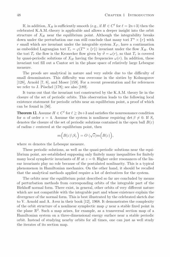
48 Chapter 1 Introduction
If, in addition, XH is sufficiently smooth (e.g., if H ∈ C for = 2n+3) then thecelebrated K.A.M.-theory is applicable and allows a deeper insight into the orbitstructure of XH near the equilibrium point. Although the integrability breaksdown under the perturbation one can still conclude that many tori Tn ×r withr small which are invariant under the integrable system XF , have a continuationas embedded Lagrangian tori Tr = ϕ(Tn × r) invariant under the flow XH . Onthe tori Tr the flow is the Kronecker flow given by ϑ = ω(r), so that Tr is coveredby quasi-periodic solutions of XH having the frequencies ω(r). In addition, theseinvariant tori fill out a Cantor set in the phase space of relatively large Lebesguemeasure.
The proofs are analytical in nature and very subtle due to the difficulty ofsmall denominators. This difficulty was overcome in the sixties by Kolmogorov[128], Arnold [7, 8], and Moser [159]. For a recent presentation and for referenceswe refer to J. Poschel [178]; see also [189].
It turns out that the invariant tori constructed by the K.A.M. theory lie in theclosure of the set of periodic orbits. This observation leads to the following localexistence statement for periodic orbits near an equilibrium point, a proof of whichcan be found in [56].
Theorem 12. Assume H ∈ C for ≥ 2n+3 and satisfies the nonresonance conditionfor α of order s = 4. Assume the system is nonlinear requiring det β = 0. If Sε
denotes the closure of the set of periodic solutions contained in the open ball B(ε)of radius ε centered at the equilibrium point, then
m(B(ε)\Sε
)= O (
√ε)m
(B(ε)
),
where m denotes the Lebesque measure.These periodic solutions, as well as the quasi-periodic solutions near the equi-
librium point, are established supposing only finitely many inequalities for finitelymany local symplectic invariants of H at z = 0. Higher order resonances of the lin-ear invariants play no role because of the postulated nonlinarity. This is a typicalphenomenon in Hamiltonian mechanics. On the other hand, it should be recalledthat the analytical methods applied require a lot of derivatives for the system.
The orbits near the equilibrium point described so far are concluded by meansof perturbation methods from corresponding orbits of the integrable part of theBirkhoff normal form. There exist, in general, other orbits of very different naturewhich are not compatible with the integrable part and whose existence explain thedivergence of the normal form. This is best illustrated by the celebrated sketch dueto V. Arnold and A. Avez in their book [12], 1968. It demonstrates the complexityof the orbit structure of a nonlinear symplectic map ϕ near a stable fixed point inthe plane R
2. Such a map arises, for example, as a transversal section map of aHamiltonian system on a three-dimensional energy surface near a stable periodicorbit. Instead of studying nearby orbits for all times, one can just as well studythe iterates of its section map.
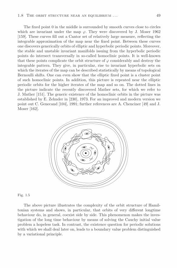
The fixed point 0 in the middle is surrounded by smooth curves close to circleswhich are invariant under the map ϕ. They were discovered by J. Moser 1962[159]. These curves fill out a Cantor set of relatively large measure, reflecting theintegrable approximation of the map near the fixed point. Between these curvesone discovers generically orbits of elliptic and hyperbolic periodic points. Moreover,the stable and unstable invariant manifolds issuing from the hyperbolic periodicpoints do intersect transversally in so-called homoclinic points. It is well-knownthat these points complicate the orbit structure of ϕ considerably and destroy theintegrable pattern. They give, in particular, rise to invariant hyperbolic sets onwhich the iterates of the map can be described statistically by means of topologicalBernoulli shifts. One can even show that the elliptic fixed point is a cluster pointof such homoclinic points. In addition, this picture is repeated near the ellipticperiodic orbits for the higher iterates of the map and so on. The dotted lines inthe picture indicate the recently discovered Mather sets, for which we refer toJ. Mather [151]. The generic existence of the homoclinic orbits in the picture wasestablished by E. Zehnder in [230], 1973. For an improved and modern version wepoint out C. Genecand [104], 1991; further references are A. Chenciner [49] and J.Moser [162].
Fig. 1.5
The above picture illustrates the complexity of the orbit structure of Hamil-tonian systems and shows, in particular, that orbits of very different longtimebehaviour do, in general, coexist side by side. This phenomenon makes the inves-tigation of the long time behaviour by means of solving the Cauchy initial valueproblem a hopeless task. In contrast, the existence question for periodic solutionswith which we shall deal later on, leads to a boundary value problem distinguishedby a variational principle.
1.8 The orbit structure near an equilibrium . . . 49
50 Chapter 1 Introduction
The local existence results described above are of analytical nature. In con-trast, the aim in Chapter 4 is to find global periodic solutions. Similarly as in thesituation near an equilibrium point, the orbit structure near a periodic solutioncan also be studied by means of a Birkhoff normal form. This normal form repre-sents an integrable approximation of the system locally near the periodic solutionwhere the linear invariants are now the Floquet multipliers of the periodic orbit.We should mention that although the qualitative methods employed in findingthese global periodic solutions are powerful, they are not sufficient to gain infor-mation about the Birkhoff invariants of these periodic solutions. Nevertheless, itis important to keep in mind that a single periodic orbit of a Hamiltonian systemcarries potential information about a nearby very rich orbit structure includingmany other periodic orbits having larger periods, quasi-periodic solutions and alsohyperbolic phenomena.
Chapter 2
Symplectic capacities
2.1 Definition and application to embeddings
In the following we introduce a special class of symplectic invariants discovered byI. Ekeland and H. Hofer in [68, 69] for subsets of R
2n. They were led to these in-variants in their search for periodic solutions on convex energy surfaces and calledthem symplectic capacities. The concept of a symplectic capacity was extended togeneral symplectic manifolds by H. Hofer and E. Zehnder in [123]. The existenceproof of these invariants is based on a variational principle; it is not intuitive,and will be postponed to the next chapter. Taking their existence for granted, theaim of this chapter is rather to deduce the rigidity of some symplectic embed-dings and, in addition, the rigidity of the symplectic nature of mappings underlimits in the supremum norm, which will give rise to the notion of a “symplectichomeomorphism”.
Definition of symplectic capacity. We consider the class of all symplectic manifolds(M,ω) possibly with boundary and of fixed dimension 2n. A symplectic capacity isa map (M,ω) → c(M,ω) which associates with every symplectic manifold (M,ω)a nonnegative number or ∞, satisfying the following properties A1–A3.A1. Monotonicity: c(M,ω) ≤ c(N, τ)if there exists a symplectic embedding ϕ : (M,ω) → (N, τ).A2. Conformality: c(M,αω) = |α|c(M,ω)for all α ∈ R, α = 0.A3. Nontriviality: c(B(1), ω0) = π = c(Z(1), ω0)for the open unit ball B(1) and the open symplectic cylinder Z(1) in the standardspace (R2n, ω0). For convenience, we recall that with the symplectic coordinates(x, y) ∈ R
2n,B(r) =
(x, y) ∈ R
2n∣∣∣ |x|2 + |y|2 < r2
andZ(r) =
(x, y) ∈ R
2n∣∣ x2
1 + y21 < r2
for r > 0. It is often convenient to replace (A3) by the following weaker axiom(A3′):A3′. Weak nontriviality: 0 < c
(B(1), ω0
)and c
(Z(1), ω0
)< ∞.
It should be pointed out that the axioms (A1)–(A3) do not determine a uniquecapacity function. There are indeed many ways to construct capacity functions as
H. Hofer and E. Zehnder, Symplectic Invariants and Hamiltonian Dynamics, 51 Modern Birkhäuser Classics, DOI 10.1007/978-3-0348-0104-1_2, © Springer Basel AG 2011
52 Chapter 2 Symplectic capacities
we shall see later on. We first illustrate the concept and deduce some simple conse-quences of the axioms (A1)–(A3). In the special case of 2-dimensional symplecticmanifolds, n = 1, the modulus of the total area
c(M,ω) := |∫
M
ω |
is an example of a symplectic capacity function. It agrees with the Lebesgue mea-sure in (R2, ω0). In contrast, if n > 1, then the symplectic invariant ( vol )
1n is ex-
cluded by axiom (A3), since the cylinder has infinite volume. If ϕ : (M,ω) → (N,σ)is a symplectic diffeomorphism between the two manifolds M and N , one appliesthe monotonicity axiom to ϕ and ϕ−1 and concludes
c(M,ω) = c(N, σ).
Therefore, the capacity is indeed a symplectic invariant. Observe also that, bymeans of the inclusion mapping, we have for open subsets of (M,ω) the mono-tonicity property
U ⊂ V =⇒ c(U) ≤ c(V ).
In order to describe some simple examples in (R2n, ω0) we start with
Lemma 1. For U ⊂ (R2n, ω0) open and λ = 0,
c(λU) = λ2c(U).
Proof. This is a consequence of the conformality axiom. The diffeomorphism
ϕ : λU → U, x → 1λ
x
satisfies ϕ∗(λ2ω0) = λ2ϕ∗ω0 = ω0. Therefore, ϕ : (λU, ω0) → (U, λ2ω0) is symplec-tic, so that c(λU, ω0) = c(U, λ2ω0) = λ2c(U, ω0) as claimed.
For the open ball of radius r > 0 in R2n we find, in particular
c(B(r)) = r2c(B(1)
)= πr2.(2.1)
Since B(r) ⊂ B(r) ⊂ B(r + ε) for every ε > 0 we conclude by monotonicity thatc(B(r)) = πr2. We see that in the special case of (R2, ω0)
c(B(r)
)= c
(B(r)
)= area
(B(r)
)
agrees with the Lebesgue measure of the disc. This can be used to show that thecapacity agrees with the Lebesgue measure for a large class of sets in R
2, as hasbeen observed by K.F. Siburg [194].

2.1 Definition and application to embeddings 53
Proposition 1. If D ⊂ R2 is a compact and connected domain with smooth bound-
ary, thenc(D,ω0) = area (D).
Proof. By removing finitely many compact curves from D, we find a simply con-nected domain D0 ⊂ D satisfying m(D0) = m(D), which in view of the uni-formization theorem is diffeomorphic to the unit disc B(1) ⊂ R
2. Therefore, thereexists a ρ > 0 and a diffeomorphism ϕ : B(ρ) → D0 satisfying, in addition,m(B(ρ)) = m(D0). Given ε > 0 we find r < ρ such that D1 := ϕ(B(r)) ⊂ D0 sat-isfies m(D1) ≥ m(D)− ε. By the theorem of Dacorogna-Moser there is, therefore,a measure preserving diffeomorphism ψ : B(r) → D1. Since this ψ is symplecticwe can estimate using the monotonicity, the invariance under symplectic diffeo-morphisms and the normalization
m(D) − ε ≤ m(D1) = m(B(r)
)= c
(B(r)
)= c(D1) ≤ c(D).
On the other hand, there exists a diffeomorphism ϕ : D → B(R)\ finitely manyopen discs of total measure ≤ ε. Choosing R appropriately we can assume, againby Dacorogna and Moser’s theorem, that ϕ is symplectic so that
c(D) ≤ c(B(R)
)= πR2 ≤ m(D) + ε.
To sum up: m(D)−ε ≤ c(D) ≤ m(D)+ε for every ε > 0 and the result follows. Clearly,
0 < c(U) < ∞
for every open and bounded set in (R2n, ω0), since U contains a small ball and iscontained in a large ball. A similar argument as for B(r) above shows for symplecticcylinders that
c(Z(r)) = πr2.(2.2)
Therefore, if an open set U satisfies
B(r) ⊂ U ⊂ Z(r)
for some r > 0, we find by the monotonicity that πr2 = c(B(r)) ≤ c(U) ≤c(Z(r)) = πr2 and hence
c(U) = πr2. (Fig. 2.1)
This demonstrates that very different (in shape, size, measure and topology)open sets can have the same capacity, if n > 1. Recall that the ellipsoids E ⊂ R
2n
introduced in the previous chapter are characterized by the (linear) symplectic
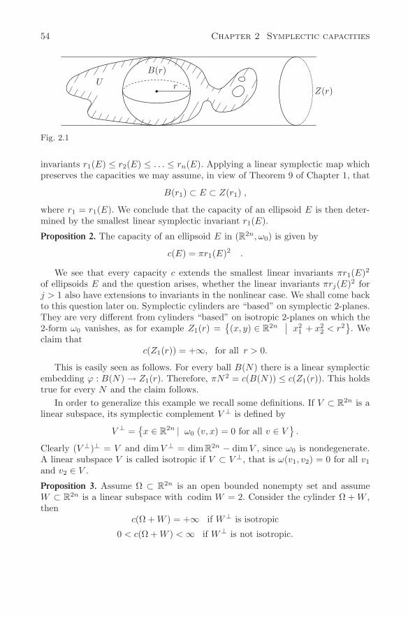
54 Chapter 2 Symplectic capacities
U
B(r)
rZ(r)
Fig. 2.1
invariants r1(E) ≤ r2(E) ≤ . . . ≤ rn(E). Applying a linear symplectic map whichpreserves the capacities we may assume, in view of Theorem 9 of Chapter 1, that
B(r1) ⊂ E ⊂ Z(r1) ,
where r1 = r1(E). We conclude that the capacity of an ellipsoid E is then deter-mined by the smallest linear symplectic invariant r1(E).
Proposition 2. The capacity of an ellipsoid E in (R2n, ω0) is given by
c(E) = πr1(E)2 .
We see that every capacity c extends the smallest linear invariants πr1(E)2
of ellipsoids E and the question arises, whether the linear invariants πrj(E)2 forj > 1 also have extensions to invariants in the nonlinear case. We shall come backto this question later on. Symplectic cylinders are “based” on symplectic 2-planes.They are very different from cylinders “based” on isotropic 2-planes on which the2-form ω0 vanishes, as for example Z1(r) =
(x, y) ∈ R
2n∣∣ x2
1 + x22 < r2
. We
claim thatc(Z1(r)) = +∞, for all r > 0.
This is easily seen as follows. For every ball B(N ) there is a linear symplecticembedding ϕ : B(N ) → Z1(r). Therefore, πN2 = c(B(N )) ≤ c(Z1(r)). This holdstrue for every N and the claim follows.
In order to generalize this example we recall some definitions. If V ⊂ R2n is a
linear subspace, its symplectic complement V ⊥ is defined by
V ⊥ =x ∈ R
2n | ω0 (v, x) = 0 for all v ∈ V
.
Clearly (V ⊥)⊥ = V and dim V ⊥ = dim R2n − dim V , since ω0 is nondegenerate.
A linear subspace V is called isotropic if V ⊂ V ⊥, that is ω(v1, v2) = 0 for all v1
and v2 ∈ V .
Proposition 3. Assume Ω ⊂ R2n is an open bounded nonempty set and assume
W ⊂ R2n is a linear subspace with codim W = 2. Consider the cylinder Ω + W ,
thenc(Ω + W ) = +∞ if W⊥ is isotropic
0 < c(Ω + W ) < ∞ if W⊥ is not isotropic.
2.1 Definition and application to embeddings 55
Proof. We may assume that Ω contains the origin. Observe that dim W⊥ = 2.Therefore, in the second case, W⊥ is a symplectic subspace and R
2n = W⊥ ⊕ W .Choosing a symplectic basis (e1, f1) in W⊥ we can, therefore, assume by a linearsymplectic change of coordinates that
W = (x, y) | x1 = y1 = 0 .
Since Ω is bounded, we have for z ∈ Ω + W , that x21 + y2
1 < N2 for some N ;consequently Ω+W ⊂ B2(N )×R
2n−2, and hence c(Ω+W ) ≤ c(B2(N )×R2n−2) =
πN2 < ∞ by (2.2). This proves the second statement. To prove the first statementwe can assume that
W = (x, y) | x1 = x2 = 0 .
There exists α > 0, so that the point (x, y) ∈ Ω + W if x21 + x2
2 < α2. Hence everyball B(R) can be symplectically embedded in Ω + W : simply define the linearsymplectic map ϕ by ϕ(x, y) = (εx, 1
εy); then ϕ(B(R)) ⊂ Ω + W provided ε > 0is sufficiently small. Consequently, by the monotonicity of a capacity, c(Ω×W ) ≥c(B(R)) = πR2. This holds true for every R > 0 so that c(Ω + W ) = +∞ asclaimed.
In view of the monotonicity property, the symplectic invariants c(M,ω) repre-sent, in particular, obstructions of symplectic embeddings. An immediate conse-quence of the axioms is the celebrated squeezing theorem of Gromov [107] whichgave rise to the concept of a capacity.
Theorem 1. (Gromov’s squeezing theorem) There is a symplectic embedding ϕ :B(r) → Z(R) if and only if R ≥ r.
Proof. If ϕ is a symplectic embedding, then using the monotonicity property ofthe capacity, together with (2.1) and (2.2), we have
πr2 = c(B(r)
)≤ c
(Z(R)
)= πR2,
and the theorem follows. The next result also illustrates the difference between volume preserving and
symplectic diffeomorphisms. We consider in (R4, ω0) with symplectic coordinates(x1, y1, x2, y2) the product of symplectic open 2-balls B(r1) × B(r2). By a linearsymplectic map we can assume that r1 ≤ r2.
Proposition 4. There is a symplectic diffeomorphism ϕ : B(r1)×B(r2) → B(s1)×B(s2) if and only if r1 = s1 and r2 = s2.
Note that, in contrast, there is a linear volume preserving diffeomorphism ψ :B(1) × B(1) → B(r) × B( 1
r) for every r > 0. As r → 0, we evidently have
c(B(r) × B
(1r
))→ 0
vol(B(r) × B
(1r
))= const.
56 Chapter 2 Symplectic capacities
Proof. Since r1 ≤ r2 we can use the diffeomorphism ϕ to define the symplecticembedding B4(r1) → B(r1) × B(r2)
ϕ→ B(s1) × B(s2) → B(s1) × R2 = Z(s1),
where the first and last mappings are the inclusion mappings. By the monotonicityof c, we conclude s1 ≥ r1. Applying the same argument to ϕ−1, we find r1 ≥ s1,so that r1 = s1. Now ϕ is volume preserving; hence r1r2 = s1s2 and the resultfollows.
Clearly, if one assumes that ϕ is smooth up to the boundary, then the conditionson the radii follow simply from the invariance of the actions |A(∂B(rj))| = πr2
j
under symplectic diffeomorphism. One might expect the same rigidity as in Propo-sition 4 to hold also in the general case of a product of n open symplectic 2-balls inR
2n. This is indeed the case, but does not follow from the capacity function c alone.Actually, the proof given in [52] is rather subtle and uses the symplectic homologytheory, as developed by A. Floer and H. Hofer in [90], see also K. Cieliebak, A.Floer, H. Hofer and K. Wysocki [52]. Finally the restrictions for symplectic em-beddings of ellipsoids mentioned in the previous chapter follow immediately fromProposition 2.
Proposition 5. Assume E and F are two ellipsoids in (R2n, ω0). If ϕ : E → F is asymplectic embedding, then
r1(E) ≤ r1(F ) .
The existence of one capacity function permits the construction of many othercapacity functions.
As an illustration we shall prove that the Gromov-width D(M,ω) which ap-pears in Gromov’s work [107] and which was explained in the introduction is asymplectic capacity satisfying (A1)–(A3). Recall that there is always a symplecticembedding ϕ : (B(ε), ω0) → (M,ω) for ε small by Darboux’s theorem and define
D(M,ω) = supπr2
∣∣∣ there is asymplectic embedding ϕ :
(B(r), ω0
)→ (M,ω)
.
Theorem 2. The Gromov-width D(M,ω) is a symplectic capacity. Moreover
D(M,ω) ≤ c(M,ω)
for every capacity function c.Because a compact symplectic manifold (M,ω) has a finite volume we conclude
D(M,ω) < ∞ for compact manifolds. This is in contrast to the special capacityfunction c0 constructed in the next chapter which can take on the value ∞ forcertain compact manifolds.
Proof. We have already verified the monotonicity axiom (A1) in the introduction.In order to verify the conformality axiom (A2), that D(M,αω) = |α|D(M,ω) forα = 0, it is sufficient to show that to every symplectic embedding
ϕ :(B(r), ω0
)→ (M,αω),
2.1 Definition and application to embeddings 57
there corresponds a symplectic embedding
ϕ :(B( r√
|α|
), ω0
)→ (M,ω),
and conversely, so that by definition of D, we conclude that D(M,αω) =|α|D(M,ω). If ϕ : (B(r), ω0) → (M,αω) is a symplectic embedding, thenϕ∗(αω) = ω0 so that
ϕ∗ω =1α
ω0.
Abbreviating ρ = r√|α|
we define the diffeomorphism ψ : B(ρ) → B(r) by setting
ψ(x) =√
|α| · x and find
ψ∗( 1
αω0
)=
|α|α
ω0.
Thus, if α > 0, the map ϕ = ϕ ψ : (B(ρ), ω0) → (M,ω) is the desired sym-plectic embedding. If α < 0 we first introduce the symplectic diffeomorphismψ0 : (B(ρ), ω0) → (B(ρ),−ω0) by setting ψ0(u, v) = (−u, v) for all (u, v) ∈ R
2n,and find the desired embedding ϕ = ϕ ψ ψ0 : (B(ρ), ω0) → (M,ω).
The verification of D(B(r), ω0) = πr2 is easy. If ϕ : B(R) → B(r) is a symplec-tic embedding, we conclude R ≤ r since ϕ is volume preserving. On the other handthe identity map induces a symplectic embedding B(r) → B(r) so that the claimfollows. Since there exists a symplectic embedding ϕ : B(R) → Z(r) if and onlyif r ≥ R by Gromov’s squeezing theorem, we conclude that D(Z(r), ω0) = πr2,hence the Gromov-width satisfies also the nontriviality axiom (A3). In order toprove the last statement of the theorem, we assume c(M,ω) to be any capacity.If ϕ : B(r) → M is a symplectic embedding we conclude by monotonicity thatπr2 = c(B(r), ω0) ≤ c(M,ω). Taking the supremum, we find D(M,ω) ≤ c(M,ω)as claimed in the theorem.
To a given capacity c one can associate its inner capacity c, defined as follows:
c(M,ω) = supc(U, ω) | U ⊂ M open and U ⊂ M\∂M
.
Correspondingly, we introduce the following
Definition. A capacity c has inner regularity at M if
c(M,ω) = c(M,ω).
Proposition 6. The function c is a capacity having inner regularity and it satisfiesc ≤ c. In addition, if d is any capacity having inner regularity and satisfying d ≤ c,then d ≤ c.
58 Chapter 2 Symplectic capacities
Proof. The proof follows readily from the definitions and the axioms for capacity.Assume, for example, that d is a symplectic capacity satisfying d ≤ c and havinginner regularity.Then
d(M) = supd(U)| U ⊂ M, U ⊂ M\∂M
≤ supc(U)| U ⊂ M, U ⊂ M\∂M
= c(M) ,
as claimed. Because it is the smallest capacity, the Gromov-width D(M,ω) has inner reg-
ularity; another example having this property is the capacity c0 introduced inChapter 3. If we consider subsets of a given manifold we can also define the con-cept of outer regularity (relative to the manifold). The outer capacity of a set isdefined as the infimum taken over the capacities of open neighborhoods of theclosure of the given set. We shall return to this concept in the next section.
2.2 Rigidity of symplectic diffeomorphisms
We consider a sequence ψj :R2n→R2n of symplectic diffeomorphisms in (R2n,ω0).
By definition, the first derivatives satisfy the identity
ψ′j(x)T J ψ′
j(x) = J , x ∈ R2n.
Therefore, if the sequence ψj converges in C1 then the limit ψ(x) = lim ψj(x) isalso a symplectic map. By contrast, we shall now assume that the sequence ψj
only converges locally uniformly to a map
ψ(x) = limj→∞
ψj(x),
which is, therefore, a continuous map. Since detψ′j(x) = 1 for every x, we find, in
view of the transformation formula for integrals, that∫f(ψ(x)
)dx =
∫f(x) dx(2.3)
for all f ∈ C∞c (R2n), so that ψ is measure preserving. Assume now that ψ is
differentiable, then evidently detψ′(x) = ±1. However it is a striking phenomenonthat ψ is even symplectic,
ψ′(x)T Jψ′(x) = J,
if it is assumed to be differentiable. Hence the symplectic nature survives undertopological limits.
2.2 Rigidity of symplectic diffeomorphisms 59
Theorem 3. Let ϕj : B(1) → (R2n, ω0) be a sequence of symplectic embeddingsconverging locally uniformly to a map ϕ : B(1) → R
2n. If ϕ is differentiable atx = 0, then ϕ′(0) = A is a symplectic map, i.e., A∗ω0 = ω0.
We see that, in general, a volume preserving diffeomorphism cannot be ap-proximated by symplectic diffeomorphisms in the C0-topology. By using, locally,Darboux charts we deduce immediately from Theorem 3
Theorem 4. (Eliashberg, Gromov) The group of symplectic diffeomorphisms of acompact symplectic manifold (M,ω) is C0-closed in the group of all diffeomor-phisms of M .
In the early seventies M. Gromov proved the alternative that the group of sym-plectic diffeomorphisms either is C0-closed in the group of all diffeomorphisms orits C0-closure is the group of volume preserving diffeomorphisms. That symplec-tic diffeomorphisms can be distinguished from volume preserving diffeomorphismsby global properties which are stable under C0-limits was announced in the earlyeighties by Y. Eliashberg in his preprint “Rigidity of symplectic and contact struc-ture”, (1981) [78], which in full form has not been published. Proofs are partiallycontained in Eliashberg [71], 1987. Gromov gave a proof of Theorem 4 in [107]using the techniques of pseudoholomorphic curves. Both Eliashberg und Gromovdeduced the C0-stability from non embedding results. In his book [108] Gromovuses so-called Nash-Moser techniques of hard implicit function theorems, whileEliashberg [71], 1987, uses an analogue of Theorem 3. Following the strategy ofI. Ekeland and H. Hofer in [68], we shall show next, that Theorem 3 is an easyconsequence of the existence of any capacity function c.
It is convenient in the following to extend the capacity to all subsets of R2n.
To do so we take a capacity function c given on the open subsets U ⊂ R2n and
define for an arbitrary subset A ⊂ R2n:
c(A) = infc(U)
∣∣A ⊂ U and U open
.
Then the monotonicity property
A ⊂ B =⇒ c(A) ≤ c(B)
holds true for all subsets of R2n. From the symplectic invariance of the capacity
on open sets, one deduces the invariance
c(ϕ(A)
)= c(A)
under every symplectic embedding ϕ defined on an open neighborhood of A.
Proof of Theorem 3. Without loss of generality we shall assume in the followingthat ϕ(0) = 0. We first claim that the linear map ϕ′(0) = A is an isomorphism.Indeed, because ϕ is differentiable at 0, we have ϕ(x) = Ax + O(|x|), so that forthe open balls Bε of radius ε > 0 and centered at 0,
m(ϕ(Bε)
)
m(Bε)−→ |det A| as ε → 0 .
60 Chapter 2 Symplectic capacities
On the other hand, because the symplectic diffeomorphisms ϕj are volume preserv-ing and ϕj → ϕ uniformly, we have m(ϕ(Bε)) = m(Bε) and hence |det A| = 1, sothat A is an isomorphism, as claimed. We shall see later on (Lemma 3) that A is anisomorphism under weaker assumption: instead of requiring ϕj to be symplectic,we shall merely require these mappings to preserve a given capacity function.
Next we claim that to prove Theorem 3, it is sufficient to show that
A∗ω0 = λω0 for some λ = 0 .(2.4)
Indeed, with ϕj we can also consider the symplectic embeddings (ϕj , id) : B(1) ×R
2n → (R2n × R2n, ω0 ⊕ ω0) and hence conclude for the derivative at (0, 0), given
by A = (A, 1), that also A∗(ω0 ⊕ ω0) = µ(ω0 ⊕ ω0) for some µ = 0. On the otherhand, in view of (2.4), A∗(ω0 ⊕ ω0) = (λω0) ⊕ ω0 and consequently µ = 1 = λ, asrequired in Theorem 4, proving our claim. In order to prove (2.4) we make use ofthe following algebraic lemma due to Y. Eliashberg [71].
Lemma 2. Assume A is a linear isomorphism satisfying A∗ω0 = λω0. Then forevery a > 0 there are symplectic matrices U and V such that U−1AV has theform
U−1AV =
a0
0a
0
∗ ∗
,
with respect to the splitting of R2n = R
2 ⊕ R2n−2 into symplectic subspaces.
Postponing the proof of the lemma, we first show that A∗ω0 = λω0 for some λ =0. Arguing by contradiction, we assume that A∗ω0 = λω0 and apply the lemma.Defining the symplectic maps ψj := U−1ϕjV in the neighborhood of the origin,we conclude that ψj → ψ := U−1ϕV locally uniformly, and ψ′(0) = U−1AV .Choosing a suitable constant a in the lemma, we have U−1AV (B(1)) ⊂ Z( 1
8) and
hence U−1ψV (B(ε)) ⊂ Z( ε4) provided ε is sufficiently small. Because ψj → ψ
locally uniformly, U−1ψjV (B(ε)) ⊂ Z( ε2) if j is sufficiently large and ε sufficiently
small. Since U−1ψjV is symplectic, we conclude by the invariance and monotonic-ity property of a capacity that c(U−1ψjV (B(ε))) = c(B(ε)) ≤ c(Z( ε
2)), whichcontradicts the nontriviality Axiom (A3). We have proved the statement in (2.4)and it remains to prove Lemma 2.
Proof of Lemma 2. Let B be the symplectic adjoint of A satisfying
ω0(Ax, y) = ω0(x, By)
for all x, y, and abbreviate ω = B∗ω0. Then ω = λω0, as is easily verified usingthe fact that A is an isomorphism. We claim that there is an x such that ω(x, ·) =λω0(x, ·) for every λ. Arguing by contradiction, we assume that for every x, thereexists a λ(x) ∈ R satisfying ω(x, ·) = λ(x)ω0(x, ·). If x = 0 there exists ξ such
2.2 Rigidity of symplectic diffeomorphisms 61
that ω0(ξ, x) = 0, since ω0 is nondegenerate. This remains true for all y in aneighborhood U(x) of x. Hence
λ(ξ) ω0(ξ, y) = ω(ξ, y) = −ω(y, ξ)
= −λ(y)ω0(y, ξ)
= λ(y)ω0(ξ, y),
which implies that λ(ξ) = λ(y) for y in a neighborhood of x. Since R2n\0 is
connected and since the function λ(x) on R2n\0 is locally constant, it is constant.
Therefore ω(x, ·) = λω0(x, ·) for x = 0 and hence for every x. This contradicts theassumption that ω = λω0 and proves our claim. Consequently there exists an xsuch that the linear map (ω0(x, ·), ω(x, ·)) : R
2n → R2 is surjective. For a given
a > 0, we therefore find an y satisfying
ω0(x, y) = 1 and ω(x, y) = a2.
Recalling ω(x, y) = ω0(Bx,By), we can choose two symplectic bases (e1, f1, . . .)and (e′1, f ′
1, . . .) such that e1 = x, f1 = y and e′1 = 1aBx, f ′
1 = 1aBy. In these bases
Be1 = ae′1, Bf1 = af ′1.
From 〈JAx, y〉 = 〈Jx, By〉 = 〈BT Jx, y〉 we read off A = −JBT J . Representingnow A in the new bases as a map from R
2n with basis (e1, f1, . . .) onto R2n with
basis (e′1, f ′1, . . .), we find the representation U−1AV of the desired form. The
symplectic matrices are defined by their column vectors as U = [e1, f1, . . .] andV = [e′1, f ′
1, . . .]. We know that symplectic diffeomorphisms preserve the capacities. Theorem 3
can, therefore, be deduced from the following, even more surprising statement forcontinuous mappings due to I. Ekeland and H. Hofer [68].
Theorem 5. Let c be a capacity. Assume ψj : B(1) → R2n is a sequence of contin-
uous mappings satisfyingc(ψj(E)) = c(E)
for all (small) ellipsoids E ⊂ B(1) and converging locally uniformly to
ψ(x) = lim ψj(x).
If ψ is differentiable at 0, then ψ′(0) = A is either symplectic or antisymplectic:
A∗ω0 = ω0 or A∗ω0 = −ω0.
Note that the mappings are not required to be invertible.In order to prove Theorem 5, we start with
62 Chapter 2 Symplectic capacities
Lemma 3. Let c be a capacity. Consider a sequence ϕj of continuous mappings inR
2n converging locally uniformly to the map ϕ. Assume that c(ϕj(E)) = c(E) forthe open ellipsoids for all j. If ϕ′(0) exists it is an isomorphism.
Proof. Arguing by contradiction, we assume that A is not surjective, so that A(R2n)is contained in a hyperplane H. Composing, if necessary, with a linear symplecticmap we may assume that
A(R2n) ⊂ H = (x, y)| x1 = 0 .(2.5)
Defining the linear symplectic map ψ by
ψ(x, y) =( 1
αx1, x2, . . . , xn, α y1, y2, . . . , yn
)
we can choose α > 0 so small that
ψA(B(1)
)⊂ B2(
116
) × R2n−2 = Z(
116
) ,
where the open 2-disc B2 on the right hand side is contained in the symplecticplane with the coordinates x1, y1. Be definition of a derivative, we have |ψϕ(x)−ψA(x)| ≤ a(|x|) |x| where a(s) → 0 as s → 0. Consequently
ψϕ(B(ε)
)⊂ Z(
ε
4)
if ε is sufficiently small. Since ψϕj converges locally uniformly to ψϕ,
ψϕj
(B(ε)
)⊂ Z(
ε
2) ,
provided j is sufficiently large. By assumption ψϕj preserves the capacity and soby monotonicity
c(B(ε)
)= c
(ψϕj(B(ε))
)≤ c
(Z(
ε
2))
=14c(B(ε)
).
This contradiction shows that A is surjective. Proof of Theorem 5. We may assume that ψ(0) = 0. By Lemma 3, A = ψ′(0) is anisomorphism and we shall prove first that A∗ω0 = λω0 for some λ = 0. Arguingby contradiction, we assume A∗ω0 = λω0 and find (by Lemma 2) symplectic mapsU and V satisfying U−1AV (B(1)) ⊂ Z( 1
8 ). Proceeding now as in Theorem 4, wedefine the sequence ϕj := U−1ψjV . Then ϕj → ϕ := U−1ψV locally uniformly,and ϕ′(0) = U−1AV . Hence ϕ(B(ε)) ⊂ Z( ε
4 ) and consequently ϕj(B(ε)) ⊂ Z( ε2 )
for j sufficiently large and ε > 0 sufficiently small. Since, by assumption on ψj ,we have c(ϕj(B(ε))) = c(B(ε)), we infer by the monotonicity of a capacity thatc(B(ε)) ≤ c(Z( ε
2 )), contradicting Axiom (A3) for a capacity.
2.2 Rigidity of symplectic diffeomorphisms 63
We have demonstrated that A∗ω0 = λω0. By conformality a linear antisymplec-tic map preserves the capacities. Composing the maps ψj and ψ with the symplec-
tic map B =(
1√λA)−1
if λ > 0 and with the antisymplectic map B =(
1√−λ
A)−1
if λ < 0, we are therefore reduced to the case
A = α 1, with α > 0
and we have to show that α = 1. If α < 1 there is a small ball and an α < r < 1such that ψj(B(ε)) ⊂ B(rε) for j large. Since ψj preserves the capacities we findc(B(ε)) = c(ψj(B(ε)) ≤ c(B(rε)) = r2c(B(ε)) which is a contradiction. In thecase α > 1 we shall show that
ψj (B(ε)) ⊃ B(rε)(2.6)
for some α > r > 1, ε small and j large, which leads to the contradictionr2c(B(ε)) = c(B(rε)) ≤ c(B(ε)). Consequently, α = 1 as claimed in the theo-rem.
To prove (2.6) we have to show that for every y ∈ B(rε) there exists anx ∈ B(ε) solving ψj(x) = y. We use an index argument based on the Brouwermapping degree. Fix 1 < r < α. Then, in view of A(B(ε)) = B(αε),
deg(B(ε), A, y) = 1,
for y ∈ B(rε), and the proof follows if we can show that
deg(B(ε), ψj , y) = deg(B(ε), A, y).
In view of the homotopy invariance of the degree, it is sufficient to verify thatthe homotopy h(t, x) = tψj(x) + (1 − t)Ax satisfies h(t, x) = y if x ∈ ∂B(ε) and0 ≤ t ≤ 1.
Recall ψ(0) = 0 and hence |ψ(x) − Ax| ≤ a(|x|)|x|, with a(s) → 0 as s → 0.Since ψj → ψ uniformly on compact sets we have, for every σ > 0 and j ≥ j0(σ)
|ψj(x) − Ax| ≤ a(|x|)|x| + σ.(2.7)
Arguing by contradiction, we assume tψj(x) + (1 − t)Ax = y for x ∈ ∂B(ε) andy ∈ B(rε). Then
t(ψj(x) − Ax) = y − Ax.
The right hand side is larger than |Ax| − |y| = αε − |y| ≥ (α − r)ε. The left handside, however is smaller than a(|ε|)ε + σ according to (2.7). Therefore, choosingσ = a(|ε|)ε and ε sufficiently small we get a contradiction, hence proving thath(t, x) = y for all 0 ≤ t ≤ 1 and all x ∈ ∂B(ε). This finishes the proof of Theorem5.
As an interesting special case we conclude from Theorem 5 the following
64 Chapter 2 Symplectic capacities
Corollary. A linear map A in R2n preserving the capacities of ellipsoids, c(A(E)) =
c(E) is either symplectic or antisymplectic.
A∗ω0 = ω0 or A∗ω0 = −ω0.
Let c be any capacity function and consider a homeomorphism h of R2n satis-
fyingc(h(E)) = c(E) for all (small) ellipsoids E.
Then, if h is in addition differentiable, we conclude from Theorem 5 that h isa diffeomorphism which is either symplectic or antisymplectic, h′(x)∗ω0 = ±ω0.This is analogous to a measure preserving homeomorphism, i.e., a homeomorphismsatisfying (2.3). Here we conclude that det h′(x) = ±1 in case h is differentiable.We see that every capacity function c singles out the distinguished group of home-omorphisms preserving the capacity of all open sets. The elements of this group ofhomeomorphisms have the additional property that they are symplectic or anti-symplectic in case they are differentiable. This group can, therefore, be viewed asa topological version of the group of symplectic diffeomorphisms. It is not knownwhether this group is closed under locally uniform limits. But the following weakerresults hold true.
Theorem 6. Assume hj : R2n → R
2n is a sequence of homeomorphisms satisfying
c(hj(E)) = c(E)
for all (resp. all small) ellipsoids E. Assume hj converges locally uniformly to ahomeomorphism h of R
2n. Then
c(h(E)) = c(E)
for all (resp. all small) ellipsoids E.
Proof. Since h−1 hj → id locally uniformly, we conclude for every ellipsoid E andevery 0 < ε < 1
h−1 hj((1 − ε)E) ⊂ E ⊂ h−1 hj((1 + ε)E),
if only j is sufficiently large. This topological fact is easily verified using the samedegree argument as above. Hence
hj((1 − ε)E) ⊂ h(E) ⊂ hj((1 + ε)E).
By monotonicity and conformality, (1−ε)2c(E) = c((1−ε)E) = c(hj((1−ε)E)) ≤c(h(E)) ≤ c(hj((1 + ε)E)) = c((1 + ε)E) = (1 + ε)2c(E). In short
(1 − ε)2c(E) ≤ c(h(E)) ≤ (1 + ε)2c(E).
This holds true for every ε > 0 so that c(h(E)) = c(E) as desired.
2.2 Rigidity of symplectic diffeomorphisms 65
In order to generalize this statement, we denote by O the family of open andbounded sets of R
2n and associate with Ω ∈ O
c(Ω) = supc(U) |U open and U ⊂ Ω
c(Ω) = infc(U) |U open and U ⊃ Ω
.
The distinguished family Oc of open sets is defined by the condition
Oc = Ω ∈ O |c (Ω) = c(Ω) .
Proposition 7. Assume hj is a sequence of homeomorphisms of R2n converging
locally uniformly to a homeomorphism h of R2n. If c(hj(U)) = c(U) for all U ∈
O and all j, then c(h(Ω)) = c(Ω) for all Ω ∈ Oc.
Proof. If Ω ∈ Oc and ε > 0 we find U , U ∈ O with U ⊃ Ω and U ⊂ Ω satisfying
c(U) ≤ c(Ω) + ε and c(U) ≥ c(Ω) − ε.
For j large we have by the above degree argument hj(U) ⊃ h(Ω) ⊃ hj(U), andhence using the monotonicity property of the capacity
c(U) = c(hj(U)) ≥ c(h(Ω)) ≥ c(hj(U)) = c(U),
so that c(Ω) + ε ≥ c(h(Ω)) ≥ c(Ω) − ε. This holds true for every ε > 0 and thetheorem is proved.
Definition. A capacity c is called inner regular, respectively, outer regular if
c(U) = c(U) resp. if c(U) = c(U)
for all U ∈ O.
Proposition 8. Assume the capacity c is inner regular or outer regular. Assume ϕj
and ϕ are homeomorphisms of R2n and
ϕj → ϕ and ϕ−1j → ϕ−1
locally uniformly. If c(ϕj(U)) = c(U) for all U ∈ O and all j, then also
c(ϕ(U)
)= c(U) for all U ∈ O.
66 Chapter 2 Symplectic capacities
Proof a) Assume c is inner regular and let Ω be open and bounded. Then if Uis open and U ⊂ Ω we have ϕj(U) ⊂ ϕ(Ω) if j is large and thus c(ϕj(U)) =c(U) ≤ c(ϕ(Ω)) so that c(U) ≤ c(ϕ(Ω)). Hence, taking the supremum we findc(Ω) ≤ c(ϕ(Ω)). Similarly one shows that c(Ω) ≤ c(ϕ−1(Ω)) for every open andbounded set Ω. Consequently, since ϕ is a homeomorphism c(Ω) = c(ϕ−1ϕ(Ω)) ≥c(ϕ(Ω)) ≥ c(Ω) and thus c(ϕ(Ω)) = c(Ω) as desired.
b) If c is outer regular and Ω is open and bounded we conclude for ε > 0that ϕj(Ω) ⊂ Uε(ϕ(Ω)) if j is sufficiently large; here Uε = x| dist (x, U) < ε.Therefore, c(Ω) = c(ϕj(Ω)) ≤ c(Uε(ϕ(Ω))) and taking the infimum on the righthand side we find c(Ω) ≤ c(ϕ(Ω)). Arguing as in the part a) we conclude thatc(ϕ(Ω)) = c(Ω) for every Ω ∈ O.
So far we have deduced from the existence of a symplectic capacity some sur-prising phenomena about symplectic mappings. Nevertheless, the notion itself isstill rather mysterious and raises many questions. It is, for example, not knownwhether the knowledge of the capacities of small sets is sufficient to understand thecapacity of larger sets. To be more precise, does, for example, a homeomorphismpreserving the capacity of small sets preserve the capacity of large sets?
We have no example of a homeomorphism which preserves one capacity but notanother. Neither do we know whether a homeomorphism preserving the capacityof open sets, also preserves the Lebesgue measure of open sets. But it is easy to seethat a homeomorphism preserving all capacities of open sets is necessarily measurepreserving. In order to prove this we first define a special embedding capacity γ.Introducing for r > 0 the open cube
Q(r) = (0, r)2n ⊂ R2n,
having edges parallel to the coordinate axis, we define
γ(M,ω) : = sup
r2 | there is a symplectic embedding ϕ : Q(r) → M.
Clearly γ is a capacity satisfying the Axioms (A1), (A2) and the weak nontrivialitycondition (A3′). It is not normalized. One can prove, by using the n-th ordercapacity function cn of Ekeland and Hofer in [69], that γ(B(r)) = 1
nπr2, moreover
γ(Z(r)) = πr2.
Proposition 9. Assume h is a homeomorphism of R2n satisfying
γ(h(Ω)
)= γ(Ω)
for all Ω ∈ O. Then h preserves the Lebesgue measure µ of open sets, i.e.,
µ(h(Ω)
)= µ(Ω)
for all Ω ∈ O.
2.2 Rigidity of symplectic diffeomorphisms 67
Proof. From the definition of γ we infer
µ(Q(r)
)= r2n = γ
(Q(r)
)n
.
Since every symplectic embedding is volume preserving we find for the capacityγ(Ω) of the open and bounded set Ω ⊂ R
2n that
µ(Ω) ≥ supr
µ(Q(r)
)= γ(Ω)n,
where the supremum is taken over those r, for which there is a symplectic embed-ding Q(r) → Ω. If Q is any open cube having its edges parallel to the coordinateaxes we conclude that
µ(Q) = γ(Q)n = γ(h(Q)
)n
≤ µ(h(Q)
).
It follows thatµ(Ω) ≤ µ
(h(Ω)
),
for every Ω ∈ O. Indeed assume Ω ∈ O; then given ε > 0 we find, in view of theregularity of the Lebesgue measure, finitely many disjoint open cubes Qj containedin Ω such that µ(Ω) − ε ≤
∑µ(Qj). Hence by the estimate above
µ(Ω) − ε ≤∑
µ(h(Qj)
)
= µ(h(⋃j
Qj))
≤ µ(h(Ω)
).
This holds true for every ε > 0 and the claim follows. By the same argument,µ(Ω) ≤ µ(h−1(Ω)) and hence µ(Ω) ≤ µ(h(Ω)) ≤ µ(h−1 h(Ω)) = µ(Ω), provingthe proposition. Corollary. If a homeomorphism of R
2n preserves all the capacities of open sets inR
2n, then it also preserves the Lebesgue measure.All our considerations so far are based on the existence of a capacity not yet
established. In the next chapter we shall construct a very special capacity functiondefined dynamically by means of Hamiltonian systems.
Chapter 3
Existence of a capacity
This chapter is devoted to the existence proof of a distinguished capacity function,denoted by c0, and introduced by H. Hofer and E. Zehnder in [123]. It is intimatelyrelated to periodic orbits of Hamiltonian systems. The capacity c0(M,ω) measuresthe minimal C0-oscillation of special Hamiltonian functions H : M → R, needed inorder to conclude the existence of a distinguished periodic orbit having small pe-riod and solving the associated Hamiltonian system XH on M . For 2-dimensionalmanifolds, c0 agrees with the total area, and in the special case of convex, open andsmooth domains U ⊂ (R2n, ω0) it is represented by a distinguished closed charac-teristic of the boundary ∂U having minimal (reduced) action equal to c0(U, ω0).This can be used, for example, to exhibit a class of compact hypersurfaces in R
2n,which are not symplectically diffeomorphic to convex ones. The proof will be basedon the action principle. The variational approach will be explained in detail. Inthe analytical framework of the Sobolev space H1/2, we shall introduce a specialminimax argument which originated in the work of P. Rabinowitz. The construc-tion of the capacity c0 completes the proof of the symplectic rigidity phenomenadescribed in Chapter 2. The special features of c0, however, will also be useful lateron for the dynamics of Hamiltonian systems.
3.1 Definition of the capacity c0
If (M,ω) is a symplectic manifold we recall that to a smooth function H : M → IRthere belongs a unique Hamiltonian vector field XH on M defined by
ω(XH(x), v) = −dH(x)(v), v ∈ TxM
and x ∈ M . A T -periodic solution x(t) of the Hamiltonian equation
x = XH(x) on M
is a solution satisfying the boundary conditions x(T ) = x(0) for some T > 0.We now single out a distinguished class of Hamiltonian functions H which lookqualitatively as depicted in the following figure 3.1.
When M has a boundary ∂M , the Hamiltonian vector field XH has compactsupport contained in the interior of M . Our guiding principle is the hope thatif the oscillation of the function H is sufficiently large, then the correspondingHamiltonian vector field possesses, independently of the size of its support, a fastperiodic solution, i.e., a periodic solution having a small period T , say 0 < T ≤ 1.
H. Hofer and E. Zehnder, Symplectic Invariants and Hamiltonian Dynamics, 69 Modern Birkhäuser Classics, DOI 10.1007/978-3-0348-0104-1_3, © Springer Basel AG 2011
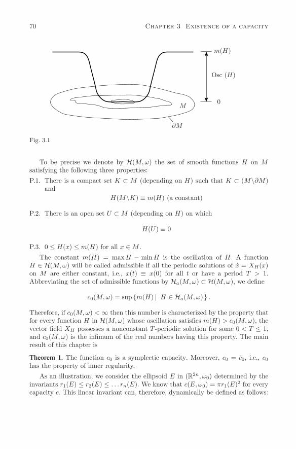
70 Chapter 3 Existence of a capacity
M
∂M
m(H)
Osc (H)
0
Fig. 3.1
To be precise we denote by H(M,ω) the set of smooth functions H on Msatisfying the following three properties:
P.1. There is a compact set K ⊂ M (depending on H) such that K ⊂ (M\∂M)and
H(M\K) ≡ m(H) (a constant)
P.2. There is an open set U ⊂ M (depending on H) on which
H(U) ≡ 0
P.3. 0 ≤ H(x) ≤ m(H) for all x ∈ M .
The constant m(H) = max H − min H is the oscillation of H. A functionH ∈ H(M,ω) will be called admissible if all the periodic solutions of x = XH(x)on M are either constant, i.e., x(t) ≡ x(0) for all t or have a period T > 1.Abbreviating the set of admissible functions by Ha(M,ω) ⊂ H(M,ω), we define
c0(M,ω) = sup m(H) | H ∈ Ha(M,ω) .
Therefore, if c0(M,ω) < ∞ then this number is characterized by the property thatfor every function H in H(M,ω) whose oscillation satisfies m(H) > c0(M,ω), thevector field XH possesses a nonconstant T -periodic solution for some 0 < T ≤ 1,and c0(M,ω) is the infimum of the real numbers having this property. The mainresult of this chapter is
Theorem 1. The function c0 is a symplectic capacity. Moreover, c0 = c0, i.e., c0
has the property of inner regularity.
As an illustration, we consider the ellipsoid E in (R2n, ω0) determined by theinvariants r1(E) ≤ r2(E) ≤ . . . rn(E). We know that c(E,ω0) = πr1(E)2 for everycapacity c. This linear invariant can, therefore, dynamically be defined as follows:
3.1 Definition of the capacity c0 71
Proposition 1. If H ∈ H(E, ω0) satisfies m(H) > πr1(E)2, then the Hamiltonianvector field XH on E possesses a nonconstant periodic solution of period 0 < T ≤1. Moreover, πr1(E)2 is the infinimum of the real numbers with this property.
Corollary. If H ∈ H(B(r), ω0) satisfies
m(H) > πr2,
then the Hamiltonian system x = XH(x) on B(r) has a nonconstant periodicsolution of period 0 < T ≤ 1.
Observe first that the statement about inner regularity c0(M,ω) = c0(M,ω)follows immediately from the definitions. We only consider the case c0(M,ω) < ∞,the case c0(M,ω) = ∞ if treated similarly. If ε > 0 then there exists H ∈ Ha(M,ω)with m(H) > c0(M,ω) − ε. Let K = supp (XH) ⊂ (M\∂M) and pick an openset U with K ⊂ U ⊂ U ⊂ (M\∂M). Clearly H ∈ Ha(U, ω) and hence c0(U, ω) ≥c0(M,ω) − ε so that c0(M,ω) = supc0(U, ω) |U ⊂ M open and U ⊂ M\∂Mwhich by definition is equal to c0(M,ω).
We have to prove that c0(M,ω) meets the axioms of a capacity c which werecall for the convenience of the reader. All the symplectic manifolds consideredare of fixed dimension 2n.
A.1. c(M,ω) ≤ c(N,σ) provided there exists a symplectic embedding ϕ : M → N .
A.2. c(M,αω) = |α| c(M,ω), α = 0.
A.3. c(Z(1), ω0) = π = c(B(1), ω0).
The first two properties follow very easily from the definition of c0.
Lemma 1. c0 satisfies the monotonicity axiom A.1.
Proof. If ϕ : M → N is a symplectic embedding we can define the map ϕ∗ :H(M,ω) → H(N,σ) as follows:
ϕ∗(H) =
H ϕ−1(x) if x ∈ ϕ(M)
m(H) if x /∈ ϕ(M).
Note that if K ⊂ M\∂M for a compact set K ⊂ M , then also ϕ(K) ⊂ N\∂N ,so that indeed ϕ∗(H) ∈ H(N, σ). Clearly m(ϕ∗(H)) = m(H), so that the lemmafollows if we show that ϕ∗(Ha(M,ω)) ⊂ Ha(N, σ). Since ϕ is symplectic ϕ∗(XH) =Xϕ∗(H) on ϕ(M) so that the flows are conjugated. In particular, the nonconstantperiodic solutions together with their periods correspond to each other.
Lemma 2. c0 satisfies the conformality axiom A.2.
Proof. Assume α = 0 and define the obvious bijection ψ : H(M,ω) → H(M,αω) byψ : H → |α|·H = Hα. Clearly m(Hα) = |α|·m(H) so that the lemma follows if weshow that ψ is also a bijection between Ha(M,ω) and Ha(M,αω). By the definition
72 Chapter 3 Existence of a capacity
of Hamiltonian vector fields (αω) (XHα, ·) = −dHα = −|α|dH = |α| ω(XH , ·).
Hence, since ω is nondegenerate
α
|α| XHα= XH on M.
Therefore, XHα= XH or XHα
= −XH and the two vector fields have the sameperiodic solutions with the same periods. Lemma 3. c0(B(1), ω0) ≥ π.
Proof. Pick 0 < ε < π, we shall construct a function H ∈ Ha(B(1)) satisfyingm(H) = π − ε, hence proving c0(B(1), ω0) ≥ π − ε. Choose a smooth functionf : [0, 1] → [0,∞) satisfying
0 ≤ f ′(t) < π
f(t) = 0 for t near 0
f(t) = π − ε for t near 1.
f
π
π − ε
t
0 1
Fig. 3.2
Define H(x) = f(|x|2) for x ∈ B(1). Then m(H) = π − ε and we claim thatH ∈ Ha(M,ω). Indeed, the Hamiltonian system
−Jx = ∇H(x) = 2f ′(|x|2)x
has the function G(x) = 12|x|2 as integral, since 〈∇G, J∇H〉 = 2 f ′ (|x|2) 〈x, Jx〉 =
0. Therefore, if x(t) is a solution, then
2 f ′ ( |x(t)|2 ) = a
is constant and the solution satisfies
−Jx = ax.
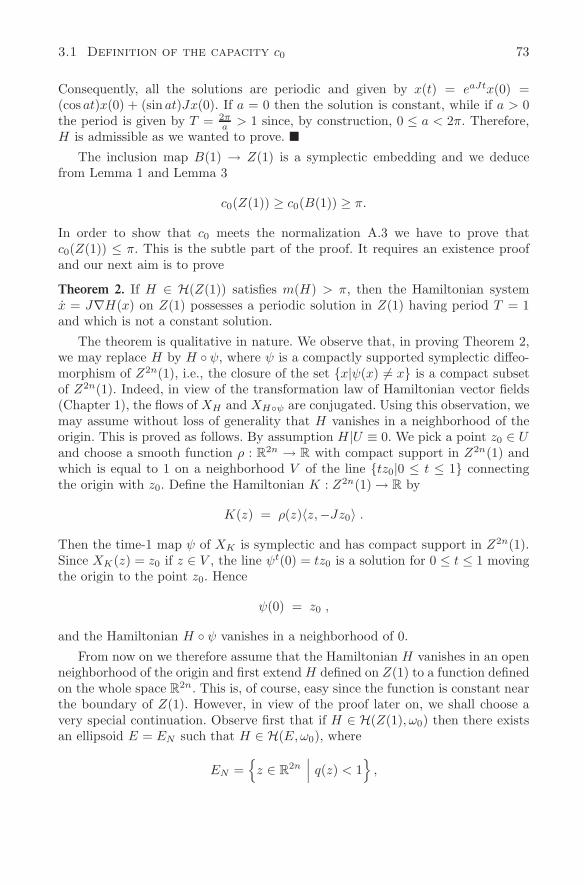
3.1 Definition of the capacity c0 73
Consequently, all the solutions are periodic and given by x(t) = eaJtx(0) =(cos at)x(0) + (sin at)Jx(0). If a = 0 then the solution is constant, while if a > 0the period is given by T = 2π
a > 1 since, by construction, 0 ≤ a < 2π. Therefore,H is admissible as we wanted to prove.
The inclusion map B(1) → Z(1) is a symplectic embedding and we deducefrom Lemma 1 and Lemma 3
c0(Z(1)) ≥ c0(B(1)) ≥ π.
In order to show that c0 meets the normalization A.3 we have to prove thatc0(Z(1)) ≤ π. This is the subtle part of the proof. It requires an existence proofand our next aim is to prove
Theorem 2. If H ∈ H(Z(1)) satisfies m(H) > π, then the Hamiltonian systemx = J∇H(x) on Z(1) possesses a periodic solution in Z(1) having period T = 1and which is not a constant solution.
The theorem is qualitative in nature. We observe that, in proving Theorem 2,we may replace H by H ψ, where ψ is a compactly supported symplectic diffeo-morphism of Z2n(1), i.e., the closure of the set x|ψ(x) = x is a compact subsetof Z2n(1). Indeed, in view of the transformation law of Hamiltonian vector fields(Chapter 1), the flows of XH and XHψ are conjugated. Using this observation, wemay assume without loss of generality that H vanishes in a neighborhood of theorigin. This is proved as follows. By assumption H|U ≡ 0. We pick a point z0 ∈ Uand choose a smooth function ρ : R
2n → R with compact support in Z2n(1) andwhich is equal to 1 on a neighborhood V of the line tz0|0 ≤ t ≤ 1 connectingthe origin with z0. Define the Hamiltonian K : Z2n(1) → R by
K(z) = ρ(z)〈z,−Jz0〉 .
Then the time-1 map ψ of XK is symplectic and has compact support in Z2n(1).Since XK(z) = z0 if z ∈ V , the line ψt(0) = tz0 is a solution for 0 ≤ t ≤ 1 movingthe origin to the point z0. Hence
ψ(0) = z0 ,
and the Hamiltonian H ψ vanishes in a neighborhood of 0.
From now on we therefore assume that the Hamiltonian H vanishes in an openneighborhood of the origin and first extend H defined on Z(1) to a function definedon the whole space R
2n. This is, of course, easy since the function is constant nearthe boundary of Z(1). However, in view of the proof later on, we shall choose avery special continuation. Observe first that if H ∈ H(Z(1), ω0) then there existsan ellipsoid E = EN such that H ∈ H(E, ω0), where
EN =
z ∈ R2n∣∣∣ q(z) < 1
,
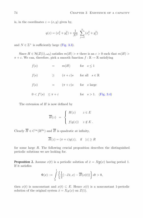
74 Chapter 3 Existence of a capacity
is, in the coordinates z = (x, y) given by,
q(z) = (x21 + y2
1) +1
N2
n∑j=2
(x2j + y2
j )
and N ∈ Z+ is sufficiently large (Fig. 3.3).
Since H ∈ H(Z(1), ω0) satisfies m(H) > π there is an ε > 0 such that m(H) >π + ε. We can, therefore, pick a smooth function f : R → R satisfying
f(s) = m(H) for s ≤ 1
f(s) ≥ (π + ε)s for all s ∈ R
f(s) = (π + ε)s for s large
0 < f ′(s) ≤ π + ε for s > 1. (Fig. 3.4)
The extension of H is now defined by
H(z) =
H(z) z ∈ E
f(q(z)) z /∈ E .
Clearly H ∈ C∞(R2n) and H is quadratic at infinity,
H(z) = (π + ε)q(z), if |z| ≥ R
for some large R. The following crucial proposition describes the distinguishedperiodic solutions we are looking for.
Proposition 2. Assume x(t) is a periodic solution of x = XH(x) having period 1.If it satisfies
Φ(x) :=
1∫
0
12〈−Jx, x〉 − H(x(t))
dt > 0,
then x(t) is nonconstant and x(t) ⊂ E. Hence x(t) is a nonconstant 1-periodicsolution of the original system x = XH(x) on Z(1).
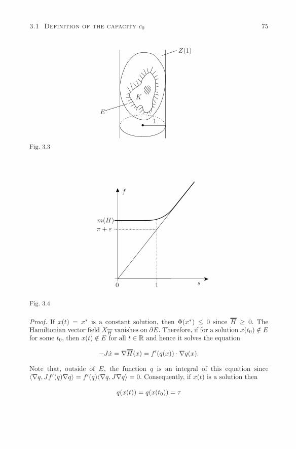
3.1 Definition of the capacity c0 75
Z(1)
E
K
1
Fig. 3.3
f
m(H)π + ε
0 1 s
Fig. 3.4
Proof. If x(t) = x∗ is a constant solution, then Φ(x∗) ≤ 0 since H ≥ 0. TheHamiltonian vector field XH vanishes on ∂E. Therefore, if for a solution x(t0) /∈ Efor some t0, then x(t) /∈ E for all t ∈ R and hence it solves the equation
−Jx = ∇H(x) = f ′(q(x)) · ∇q(x).
Note that, outside of E, the function q is an integral of this equation since〈∇q, Jf ′(q)∇q〉 = f ′(q)〈∇q, J∇q〉 = 0. Consequently, if x(t) is a solution then
q(x(t)) = q(x(t0)) = τ
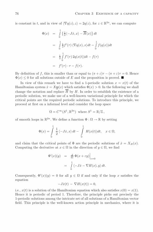
76 Chapter 3 Existence of a capacity
is constant in t, and in view of 〈∇q(z), z〉 = 2q(z), for z ∈ R2n, we can compute
Φ(x) =1∫0
12 〈−Jx, x〉 − H(x)
dt
=1∫0
12f ′(τ) 〈∇q(x), x〉dt −
1∫0
f(q(x))dt
= 12
1∫0
f ′(τ) 2q(x(t))dt − f(τ)
= f ′(τ) · τ − f(τ).
By definition of f , this is smaller than or equal to (π + ε)τ − (π + ε)τ = 0. HenceΦ(x) ≤ 0 for all solutions outside of E and the proposition is proved.
In view of this remark we have to find a 1-periodic solution x = x(t) of theHamiltonian system x = XH(x) which satisfies Φ(x) > 0. In the following we shallchange the notation and replace H by H. In order to establish the existence of aperiodic solution, we make use of a well-known variational principle for which thecritical points are the required periodic solutions. To introduce this principle, weproceed at first on a informal level and consider the loop space
Ω = C∞(S1, R2n) where S1 = R/Z ,
of smooth loops in R2n. We define a function Φ : Ω → R by setting
Φ(x) =
1∫
0
12〈−Jx, x〉 dt −
1∫
0
H(x(t))dt, x ∈ Ω,
and claim that the critical points of Φ are the periodic solutions of x = XH(x).Computing the derivative at x ∈ Ω in the direction of y ∈ Ω, we find
Φ′(x)(y) = ddε
Φ(x + εy)∣∣∣ε=0
=1∫0
〈−Jx −∇H(x), y〉 dt.
Consequently, Φ′(x)(y) = 0 for all y ∈ Ω if and only if the loop x satisfies theequation
−Jx(t) − ∇H(x(t)) = 0,
i.e., x(t) is a solution of the Hamiltonian equation which also satisfies x(0) = x(1).Hence it is periodic of period 1. Therefore, the principle picks out precisely the1-periodic solutions among the intricate set of all solutions of a Hamiltonian vectorfield. This principle is the well-known action principle in mechanics, where it is
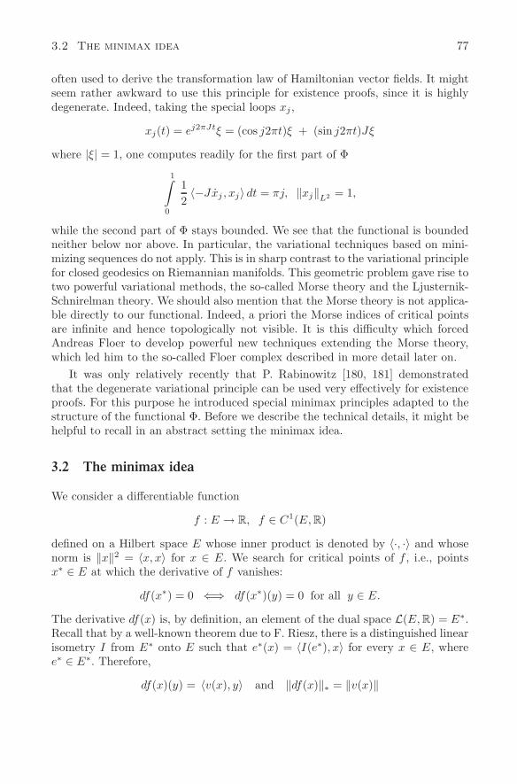
3.2 The minimax idea 77
often used to derive the transformation law of Hamiltonian vector fields. It mightseem rather awkward to use this principle for existence proofs, since it is highlydegenerate. Indeed, taking the special loops xj ,
xj(t) = ej2πJtξ = (cos j2πt)ξ + (sin j2πt)Jξ
where |ξ| = 1, one computes readily for the first part of Φ
1∫
0
12〈−Jxj , xj〉 dt = πj, ‖xj‖L2 = 1,
while the second part of Φ stays bounded. We see that the functional is boundedneither below nor above. In particular, the variational techniques based on mini-mizing sequences do not apply. This is in sharp contrast to the variational principlefor closed geodesics on Riemannian manifolds. This geometric problem gave rise totwo powerful variational methods, the so-called Morse theory and the Ljusternik-Schnirelman theory. We should also mention that the Morse theory is not applica-ble directly to our functional. Indeed, a priori the Morse indices of critical pointsare infinite and hence topologically not visible. It is this difficulty which forcedAndreas Floer to develop powerful new techniques extending the Morse theory,which led him to the so-called Floer complex described in more detail later on.
It was only relatively recently that P. Rabinowitz [180, 181] demonstratedthat the degenerate variational principle can be used very effectively for existenceproofs. For this purpose he introduced special minimax principles adapted to thestructure of the functional Φ. Before we describe the technical details, it might behelpful to recall in an abstract setting the minimax idea.
3.2 The minimax idea
We consider a differentiable function
f : E → R, f ∈ C1(E, R)
defined on a Hilbert space E whose inner product is denoted by 〈·, ·〉 and whosenorm is ‖x‖2 = 〈x, x〉 for x ∈ E. We search for critical points of f , i.e., pointsx∗ ∈ E at which the derivative of f vanishes:
df(x∗) = 0 ⇐⇒ df(x∗)(y) = 0 for all y ∈ E.
The derivative df(x) is, by definition, an element of the dual space L(E, R) = E∗.Recall that by a well-known theorem due to F. Riesz, there is a distinguished linearisometry I from E∗ onto E such that e∗(x) = 〈I(e∗), x〉 for every x ∈ E, wheree∗ ∈ E∗. Therefore,
df(x)(y) = 〈v(x), y〉 and ‖df(x)‖∗ = ‖v(x)‖
78 Chapter 3 Existence of a capacity
where v(x) ∈ E is uniquely determined by df(x). It is called the gradient of f atx (with respect to the inner product 〈 ·, · 〉) and denoted by
v(x) = ∇f(x) ∈ E.
The critical points of f are the zeros of the gradient function x → ∇f(x) in E.Using a dynamical approach, we interpret the critical points of f as the equilibriumpoints of the gradient equation
x = −∇f(x), x ∈ E.
This is an ordinary differential equation on E, and we shall assume now that ithas a global flow ϕt(x), i.e., that we can solve the Cauchy initial value problemuniquely and for all times t ∈ R:
ddtϕ
t(x) = −∇f (ϕt(x))
ϕ0(x) = x,
for all initial conditions x ∈ E. Such a global flow does exist, for example, if thereis a constant M ≥ 0 such that ‖∇f(x)−∇f(y)‖ ≤ M‖x− y‖ for all x, y ∈ E, asis, of course, well-known. The crucial property of the gradient flow is that f(ϕt(x))decreases along nonconstant solutions ϕt(x). This follows immediately from thedefinitions; indeed
ddsf (ϕs(x)) = df (ϕs(x))
(ddsϕs(x)
)
= df (ϕs(x)) (−∇f(ϕs(x)))
= − 〈∇f (ϕs(x)) ,∇f (ϕs(x))〉 .
In particular,
f(ϕt(x)
)− f(x) =
t∫
0
d
dsf (ϕs(x)) ds = −
t∫
0
‖∇f (ϕs(x)) ‖2ds.(3.1)
Since E is not compact we cannot expect f to have any critical points unless weimpose additional conditions on f , as the example f(x) = e−x on x ∈ R alreadyshows. The following strong compactness condition goes back to Palais and Smale[175] and guarantees a critical point in many variational problems.
Definition. f is said to satisfy P.S., if every sequence xj ∈ E satisfying
∇f(xj) → 0 in E and |f(xj)| ≤ c < ∞,
for some c ≥ 0, possesses a convergent subsequence. Since f is assumed to be C1,the limit of this subsequence is a critical point of f .
3.2 The minimax idea 79
If F is a family of subsets F ⊂ E one defines the minimax c(f,F) belongingto f and F by
c(f,F) = infF∈F
supx∈F
f(x) ∈ R ∪ ∞ ∪ −∞
Minimax Lemma. Assume f ∈ C1(E, R) and F meet the following conditions:
(i) f satisfies P.S.
(ii) x = −∇f(x) defines a global flow ϕt(x)
(iii) The family F is positively invariant under the flow, i.e., if F ∈ F thenϕt(F ) ∈ F for every t ≥ 0
(iv) −∞ < c(f,F) < ∞.
Then the real number, c(f,F) is a critical value of f , i.e., there exists x∗ ∈ Esatisfying
∇f(x∗) = 0 and f(x∗) = c(f,F).
Proof. Abbreviating c = c(f,F) which, by assumption, is a real number, we shallshow that for every ε > 0 there exists an x ∈ E satisfying
c − ε ≤ f(x) ≤ c + ε and ‖ ∇f(x) ‖ ≤ ε.
Then choosing εj = 1/j we find a sequence xj which has, by the P.S. condition,a convergent subsequence whose limit satisfies ∇f(x∗) = 0 and f(x∗) = c, henceproving the Lemma. Arguing by contradiction we find an ε > 0 such that
‖ ∇f(x) ‖ > ε(3.2)
for all x satisfying c − ε ≤ f(x) ≤ c + ε. By the definition of c, there exists anF ∈ F satisfying
supx∈F
f(x) ≤ c + ε.(3.3)
Pick a point x ∈ F ; then f(x) ≤ c + ε and we claim that the solution ϕt(x)satisfies f(ϕt∗(x)) ≤ c − ε if t∗ = 2/ε. Indeed, if f(ϕt(x)) ≤ c − ε for some0 ≤ t ≤ t∗ there is nothing to prove since f(ϕt(x)) is decreasing. Assume now, bycontradiction, that f(ϕt(x)) > c − ε for all 0 ≤ t ≤ t∗. Then by, (3.2), we have||∇f(ϕt(x))|| ≥ ε, for 0 ≤ t ≤ t∗, and hence, by (3.1), f(ϕt(x)) ≤ f(x) − ε2t, sothat f(ϕt∗(x)) ≤ c + ε − ε2t∗ = c − ε, a contradiction. Setting F ∗ = ϕt∗(F ) wehave shown that
supx∈F∗
f(x) ≤ c − ε .
Since, by assumption, F ∗ ∈ F , this estimate contradicts the definition of c.
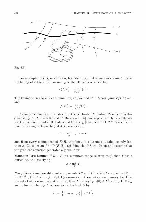
80 Chapter 3 Existence of a capacity
c + ε
c
c − ε
F
F ∗
Fig. 3.5
For example, if f is, in addition, bounded from below we can choose F to bethe family of subsets x consisting of the elements of E so that
c(f,F
)= inf
x∈Ef(x).
The lemma then guarantees a minimum, i.e., we find x∗ ∈ E satisfying ∇f(x∗) = 0and
f(x∗) = inf
x∈Ef(x).
As another illustration we describe the celebrated Mountain Pass Lemma dis-covered by A. Ambrosetti and P. Rabinowitz [6]. We reproduce the visually at-tractive version found in R. Palais and C. Terng [174]. A subset R ⊂ E is called amountain range relative to f if it separates E, if
α := infR
f > −∞
and if on every component of E\R, the function f assumes a value strictly lessthan α. Consider an f ∈ C1(E, R) satisfying the P.S. condition and assume thatthe gradient equation generates a global flow.
Mountain Pass Lemma. If R ⊂ E is a mountain range relative to f , then f has acritical value c satisfying
c ≥ infR
f.
Proof. We choose two different components E0 and E1 of E\R and define Ejα =
x ∈ Ej | f(x) < α for j = 0, 1. By assumption, these sets are not empty. Let Γ bethe set of all continuous paths γ : [0, 1] → E satisfying γ(0) ∈ E0
α and γ(1) ∈ E1α
and define the family F of compact subsets of E by
F =
image (γ)∣∣∣ γ ∈ Γ
.
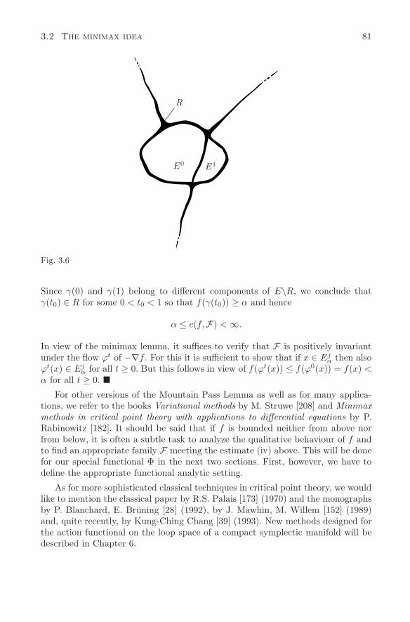
3.2 The minimax idea 81
R
E0 E1
Fig. 3.6
Since γ(0) and γ(1) belong to different components of E\R, we conclude thatγ(t0) ∈ R for some 0 < t0 < 1 so that f(γ(t0)) ≥ α and hence
α ≤ c(f,F) < ∞.
In view of the minimax lemma, it suffices to verify that F is positively invariantunder the flow ϕt of −∇f . For this it is sufficient to show that if x ∈ Ej
α then alsoϕt(x) ∈ Ej
α for all t ≥ 0. But this follows in view of f(ϕt(x)) ≤ f(ϕ0(x)) = f(x) <α for all t ≥ 0.
For other versions of the Mountain Pass Lemma as well as for many applica-tions, we refer to the books Variational methods by M. Struwe [208] and Minimaxmethods in critical point theory with applications to differential equations by P.Rabinowitz [182]. It should be said that if f is bounded neither from above norfrom below, it is often a subtle task to analyze the qualitative behaviour of f andto find an appropriate family F meeting the estimate (iv) above. This will be donefor our special functional Φ in the next two sections. First, however, we have todefine the appropriate functional analytic setting.
As for more sophisticated classical techniques in critical point theory, we wouldlike to mention the classical paper by R.S. Palais [173] (1970) and the monographsby P. Blanchard, E. Bruning [28] (1992), by J. Mawhin, M. Willem [152] (1989)and, quite recently, by Kung-Ching Chang [39] (1993). New methods designed forthe action functional on the loop space of a compact symplectic manifold will bedescribed in Chapter 6.
82 Chapter 3 Existence of a capacity
3.3 The analytical setting
Let H ∈ C∞(R2n, R) denote the special Hamiltonian function introduced in Sec-tion 3.1. It vanishes on an open neighborhood of the origin and satisfies
H(z) = Q(z), |z| ≥ R ,(3.4)
with the quadratic form Q(z) = (π + ε)q(z), z ∈ R2n. We shall translate these
properties of the Hamiltonian into properties of the corresponding functional Φon an appropriate Hilbert space. Recall that on the space Ω = C∞(S1, R2n) ofsmooth loops Φ is defined by
Φ(x) =
1∫
0
12 〈−Jx, x〉dt −
1∫
0
H (x(t)) dt, x ∈ Ω.(3.5)
In order to find the convenient Hilbert space, we represent the periodic loopsx ∈ C∞(S1, R2n) by their Fourier-series
x(t) =∑k∈Z
ek2πJt xk , xk ∈ R2n(3.6)
which converge, together with all their derivatives, in the supremum norm. Con-sidering first the dominant part of Φ which reflects the symplectic structure, weabbreviate
a(x, y) =
1∫
0
12〈−Jx, y〉dt, x, y ∈ Ω.(3.7)
Then, inserting the Fourier expansions of x, y ∈ Ω into a(x, y), and observing that
1∫
0
〈ej2πJt xj , ek2πJt yk〉dt = δjk
〈xj , yk〉,
one obtains
2a(x, y) = 2π∑j∈Z
j 〈xj , yj〉(3.8)
= 2π∑j>0
|j| 〈xj , yj〉 − 2π∑j<0
|j| 〈xj , yj〉.
Consequently, a(x, y) can be defined as a continuous bilinear form on the largerspace H1/2 = H1/2(S1) which is a special Sobolev space. Recall that the spaces
3.3 The analytical setting 83
Hs = Hs(S1) for s ≥ 0 are defined by
Hs =
x ∈ L2(S1)
∣∣∣ ∑j∈Z
|j|2s|xj |2 < ∞
wherex =
∑j∈Z
ej2πJtxj , xj ∈ R2n
is the Fourier series of x which converges in L2(S1). The space Hs is a Hilbertspace with inner product and associated norm defined by
〈x, y〉s = 〈x0, y0〉 + 2π∑k∈Z
|k|2s〈xk, yk〉
‖x‖2s = 〈x, x〉s,
for x, y ∈ Hs. Note that the norm ||x||0 is equivalent to the L2-norm. We shalldenote the distinguished Hilbert space H1/2 which will be the underlying space ofour functional by
E ≡ H1/2
〈 , 〉 ≡ 〈 , 〉 12
and ‖ ‖ = ‖ ‖ 12.
There is an orthogonal splitting of E
E = E− ⊕ E0 ⊕ E+
into the spaces of x ∈ E having only Fourier coefficients for j < 0, j = 0, j > 0.The corresponding orthogonal projections are denoted by P−, P 0, P+. Therefore,every x ∈ E has a unique decomposition
x = x− + x0 + x+.
In view of (3.8) we define for x, y ∈ E
a(x, y) = 12 〈x+, y+〉 − 1
2〈x−, y−〉(3.9)
= 12 〈(P+ − P−)x, y〉,
which is a continuous bilinear form on E and which agrees for x, y ∈ C∞(S1, R2n)with (3.7). The function a : E → R, defined by
a(x) = a(x, x) = 12‖x+‖2 − 1
2‖x−‖2,(3.10)
is differentiable with derivative
da(x) (y) = 〈(P+ − P−)x, y〉,
84 Chapter 3 Existence of a capacity
so that the gradient of a is
∇a(x) = (P+ − P−)x = x+ − x− ∈ E,(3.11)
at every point x ∈ E.Next we point out some useful properties of the spaces Hs needed later on.
Clearly the spaces decrease,
Ht ⊂ Hs ⊂ H0 for t ≥ s ≥ 0,
while the norms increase:
‖x‖t ≥ ‖x‖s ≥ ‖x‖0 for x ∈ Ht.
In particular, the inclusion maps I : Ht → Hs for t ≥ s are continuous.
Proposition 3. Assume t > s ≥ 0. Then the inclusion map I : Ht → Hs is compact,i.e., it maps bounded sets of Ht onto relatively compact subsets of Hs.
Proof. The continuous linear operator PN : Ht → Hs defined by
PN x =∑
|k|≤N
ek2πJt xk
has finite dimensional range and hence is a compact operator. The estimate
‖(PN − I)x‖2s = ‖
∑|k|>N
ek2πJt xk‖2s
= 2π∑
|k|>N
|k|2s |xk|2 = 2π∑
|k|>N
|k|2(s−t) |k|2t |xk|2
≤ N2(s−t) 2π∑
|k|>N
|k|2t |xk|2 ≤ N2(s−t) ‖x‖2t
shows that PN → I in the operator norm, i.e., the norm of L(Hs,Ht). Conse-quently I is also compact, which is well-known and easily seen as follows. Letε > 0 and choose N so large that ‖PN − I‖ < ε/2 in the operator-norm. If B isthe unit ball in Ht, then PN (B) ⊂ Hs is covered by finitely many balls of radiusε/2 which are centered at the points y1, y2, . . . , ym ∈ Hs. Hence, if x ∈ B we findan yj satisfying ‖PN (x) − yj‖s < ε/2 and together with ‖PN (x) − I(x)‖s < ε/2this implies that ‖I(x) − yj‖s < ε. Thus I(B) is covered by finitely many ballsof radius ε > 0. This holds true for every ε > 0 and we conclude that I(B) isrelatively compact in Hs.
The set C∞(S1, R2n) is dense in Hs for every s ≥ 0. However, not all elements ofH1/2 are represented by continuous functions. In order to find continuous functionsthe following proposition will be helpful.
3.3 The analytical setting 85
Proposition 4. Assume s > 12 . If x ∈ Hs then x ∈ C(S1). Moreover, there is a
constant c = cs such that
sup0≤t≤1
|x(t)| ≤ c ‖x‖s , x ∈ Hs(S1).
Proof. We show that the Fourier series
x =∑
k
ek2πJt xk,
which converges in L2, also converges in the sup-norm. This follows from theestimates:
∑k =0
∣∣ek2πJt xk
∣∣ =∑k =0
∣∣xk
∣∣ =∑k =0
|k|−s |k|s |xk|
≤(∑
k =0
1|k|2s
) 12 ·(∑
k =0
|k|2s |xk|2) 1
2
≤ c ‖x‖s,
where we have used that 2s > 1. The same argument shows that, more generally, if s > 1
2 + r for an integer r,then x ∈ Hs belongs to Cr(S1) and
sup∣∣Djx(t)
∣∣ ≤ c ‖x‖s , x ∈ Hs(S1) .0 ≤ j ≤ r0 ≤ t ≤ 1
This is again a special case of the Sobolev embedding theorem. In view of Propo-sition 3, the inclusion map
j : H1/2 −→ L2(3.12)
is compact. Its adjoint operator
j∗ : L2 −→ H1/2(3.13)
is, as usual, defined by(j(x), y
)L2
= 〈x, j∗(y)〉 12
(3.14)
for all x ∈ H1/2 and y ∈ L2. The following property of j∗ will be useful later on.
86 Chapter 3 Existence of a capacity
Proposition 5.j∗(L2) ⊂ H1 and ‖j∗(y)‖1 ≤ ‖y‖L2 .
The map j∗ factors: L2 → H1 → H1/2, thus we have verified using Proposition3 that j∗ is a compact operator. This follows also from the compactness of j, as iswell-known.
Proof. By definition of the adjoint∑
k
〈xk, yk〉 = 〈x0, j∗(y)0〉 + 2π
∑k
|k| 〈xk, j∗(y)k〉
for x ∈ H1/2 ⊂ L2 and y ∈ L2. One reads off the following formula for j∗
j∗(y) = y0 +∑k =0
12π |k| ek2πJt yk,
if y ∈ L2. The estimate‖j∗(y)‖1 ≤ ‖y‖L2
is now obvious. Coming back to the functional Φ, we next study the function
b(x) =
1∫
0
H(x(t)
)dt ,
recalling that H vanishes in a neighborhood of the origin. In view of |H(z)| ≤M |z|2, for all z ∈ R
2n, this map b is defined for x ∈ L2 and hence also forx ∈ E ⊂ L2. If we consider b as a function on L2, we shall denote it by b, so that,with the inclusion map j : E → L2, we can write
b(x) = b(j(x)
), x ∈ E.(3.15)
In order to prove that b : L2 → R is differentiable, we start from the identity
H(z + ξ) = H(z) + 〈∇H(z), ξ〉 +
1∫
0
〈∇H(z + tξ) −∇H(z), ξ〉 dt(3.16)
for z, ξ ∈ R2n. Since |Hzz(z)| ≤ M the last term is ≤ M |ξ|2. Assume now that
x ∈ L2 then ∇H(x) = ∇H(x(t)) ∈ L2 in view of |∇H(z)| ≤ M |z| for all z ∈ R2n.
Therefore, given x and h ∈ L2, we find by integration
b(x + h) = b(x) +
1∫
0
〈∇H(x), h〉 dt + R(x, h).
3.3 The analytical setting 87
Moreover, |R(x, h)| ≤ M ‖h‖2L2 . This estimate shows that b is differentiable with
derivative at x given by
db(x)(h) =1∫0
〈∇H(x), h〉 dt = (∇H(x), h)L2
= (∇b(x), h)L2 .
For the gradient (with respect to L2) we read off ∇b(x) = ∇H(x) ∈ L2. Thederivative of b : E → R is in view of (3.14) given by
〈∇b(x), y〉 = db(x)(y) = db (j(x)) (j(y))
=(∇b(j(x)
), j(y)
)L2
= 〈j∗∇b(j(x)), y〉 .
Therefore,
∇b(x) = j∗ ∇b(j(x)
)= j∗ ∇H(x) .(3.17)
Lemma 4. The map b : E → R is differentiable. Its gradient ∇b : E → E iscontinuous and maps bounded sets into relatively compact sets. Moreover,
‖∇b(x) −∇b(y)‖ ≤ M‖x − y‖
and |b(x)| ≤ M ||x||2L2 for all x, y ∈ E.
Proof. Clearly x → ∇H(x) is globally Lipschitz continuous on L2 and maps,therefore, bounded sets into bounded sets. The first claim follows from (3.17),since j∗ : L2 → E is compact. Moreover,
‖∇b(x) − ∇b(y)‖ 12
= ‖j∗(∇H(x) −∇H(y)
)‖ 1
2
≤ ‖∇H(x) −∇H(y)‖L2 ≤ M ‖x − y‖L2
≤ M ‖x − y‖ 12.
The last estimate follows from |H(z)| ≤ M |z|2, for all z ∈ R2n.
It should be mentioned that b ∈ C∞(E, R) provided H ∈ C∞(R2n, R). This isreadily seen by using the Taylor formula together with the nontrivial fact that Eis continuously embedded in Lp for every p ≥ 1 which is proved in the Appendix.To keep our presentation elementary we shall, however, not use this observationhere. Summarizing the discussion so far, we have extended Φ from the space Ω ofsmooth loops to the Hilbert space E ⊃ Ω by
Φ(x) = a(x) − b(x) , x ∈ E.
88 Chapter 3 Existence of a capacity
This function Φ : E → R is differentiable and its gradient is given by
∇Φ(x) = x+ − x− −∇b(x).
We are interested in classical solutions of differential equations. It is, therefore,important to observe now that a critical point of Φ is not simply an element in Ewhich might not even be a continuous function, but it is actually a smooth periodicsolution of the Hamiltonian equation XH having period 1. Indeed the following“regularity” statement holds true.
Lemma 5. Assume x ∈ E is a critical point, ∇Φ(x) = 0. Then x ∈ C∞(S1).Moreover, it solves the Hamiltonian equation
x(t) = J∇H(x(t)
), 0 ≤ t ≤ 1,
so that x ∈ Ω is a 1-periodic solution.
Proof. Represent x and ∇H(x) ∈ L2 by their Fourier expansions in L2
x =∑
ek 2π Jt xk
∇H(x) =∑
ek 2π Jt ak.
By assumption dΦ(x)(v) = 0.Hence, using 〈∇b(x), v〉 = 〈j∗∇H(x), v〉 = (∇H(x), v)L2 ,
〈(P+ − P−)x, v〉 =
1∫
0
〈∇H(x), v〉 dt
for all v ∈ E. Choosing the test functions v(t) = ek2πJt v, we find
2πk xk = ak , k ∈ Z(3.18)
and a0 = 0. We infer that∑
|k|2 |xk|2 ≤∑
|ak|2 < ∞,
so that x ∈ H1 and by Proposition 4, the element x ∈ E belongs to C(S1).Consequently ∇H(x(t)) ∈ C(S1), and, therefore,
ξ(t) =
t∫
0
J∇H(x(t)
)dt ∈ C1(R).
Comparing the Fourier coefficients we find in view of (3.18), that ξ(t) = x(t)−x(0),hence x belongs to C1(S1) and also solves the equation x(t) = J∇H(x(t)). The
3.3 The analytical setting 89
right hand side of the equation is in C1, hence x ∈ C2, and iterating this argumentwe conclude that x ∈ C∞(S1) as claimed.
The careful choice of the asymptotic behaviour of the Hamiltonian function Himplies that XH has, in the region of R
2n where |z| is large, no periodic solutionsof period 1. From this dynamical behaviour, we shall conclude that Φ satisfies theP.S. condition.
Lemma 6. Every sequence xj ∈ E satisfying ∇Φ(xj) → 0 contains a convergentsubsequence. In particular, Φ satisfies the P.S. condition.
Proof. Assume ∇Φ(xj) → 0 so that
x+j − x−
j −∇b(xj) → 0.(3.19)
Recall the splitting xj = x−j + x0
j + x+j . If xj is bounded in E, then x0
j ∈ R2n is
bounded and we conclude in view of the compactness of ∇b that there exists aconvergent subsequence. To prove that xj is bounded we argue by contradictionand assume ‖xj‖ → ∞. Define
yk =xk
‖xk‖
so that ||yk|| = 1. By assumption, using (3.17),
(P+ − P−)yk − j∗(
1‖xk‖
∇H(xk))
→ 0.
Since |∇H(z)| ≤ M |z| the sequence
∇H(xk)‖xk‖
∈ L2
is bounded in L2. Since j∗ : L2 → E is compact, (P+−P−)yk is relatively compact,and since, in addition, y0
k is bounded in R2n, the sequence yk is relatively compact
in E. After taking a subsequence we can assume yk → y in E and hence yk → yin L2.
‖∇H(xk)‖xk‖
− ∇Q(y)‖L2 ≤ 1‖xk‖
‖∇H(xk) − ∇Q(xk)‖L2 + ‖∇Q(yk − y)‖L2 .
Since |∇H(z) − ∇Q(z)| ≤ M for all z ∈ R2n and since ∇Q defines a continuous
linear operator of L2, we conclude
∇H(xk)‖xk‖
→ ∇Q(y) in L2.
Consequently,
∇b(xk)‖xk‖
= j∗(∇H(xk)‖xk‖
)→ j∗
(∇Q(y)
)in E.
90 Chapter 3 Existence of a capacity
This implies that y ∈ E solves the linear equation in E
y+ − y− − j∗ ∇Q(y) = 0
‖y‖ = 1.
As in Lemma 5 one verifies that y belongs to C∞(S1, R2n) and also solves thelinear Hamiltonian equation
y(t) = XQ
(y(t)
)
y(0) = y(1).
Recall now that Q = (π + ε)q, and q(z) = (x21 +y2
1)+ 1N2
n∑j=2
(x2j +y2
j ). We see that
the symplectic 2-planes xj , yj are filled with periodic solutions of XQ havingperiods T = 1. Since the linear equation does not admit any nontrivial periodicsolutions of period 1 we conclude y(t) = 0. This contradicts ‖y‖ = 1 and weconclude that the sequence xk must be bounded.
The gradient equation
x = −∇Φ(x), x ∈ E
is in view of Lemma 4 globally Lipschitz continuous and, therefore, defines a uniqueglobal flow
R × E → E : (t, x) → ϕt(x) ≡ x · t,
which maps bounded sets into bounded sets. All this is well-known from the the-ory of ordinary differential equations. Our flow has, in addition, a compactnessproperty which will be crucial for the topological arguments in the next section.
Lemma 7. The flow of x = −∇Φ(x) admits the representation
x · t = et x− + x0 + e−t x+ + K(t, x),(3.20)
where K : R×E → E is continuous and maps bounded sets into precompact sets.
Proof. Prompted by the variation of constant formula, we define K by
K(t, x) = −t∫
0
(et−s P− + P 0 + e−t+s P+
)∇b (x · s) ds.
We have to verify that K has the desired properties. Abbreviating the right handside of (3.20) by y(t), one verifies readily that
y(t) = (P− − P+)y(t) − ∇b(x · t).
3.4 The existence of a critical point 91
Since y(0) = x, the function ξ(t) = y(t) − x · t solves the linear equation
ξ(t) = (P− − P+) ξ(t) and ξ(0) = 0.
By the uniqueness of the initial value problem ξ(t) = 0 so that y(t) = x · t asrequired. In view of (3.16) and (3.17) we can write
K(t, x) = j∗
−
t∫
0
(et−s P− + P 0 + e−t+s P+
)∇H
(j(x · s)
)ds
.
Abbreviating the map in the bracket by k(t, x) then k : R×E → L2 is continuousand maps bounded sets into bounded sets. By Proposition 5, the map j∗ : L2 →E maps bounded sets into precompact sets and, therefore, K has the desiredproperties.
To sum up this rather technical section we have extended the classical Hamilto-nian functional originally given on the loop space of smooth loops, and constructeda functional Φ ∈ C1(E, R) on the Hilbert space E. Its critical points, if there areany, are smooth periodic solutions of the Hamiltonian equations with period 1.The functional Φ has, in addition, crucial compactness properties. It remains tofind a special critical point x∗ ∈ E of Φ satisfying Φ(x∗) > 0. This will be done inthe next section.
3.4 The existence of a critical point
A special minimax argument will guarantee the existence of a special critical pointof the functional Φ introduced in the previous section:
Φ(x) = a(x) − b(x)
= 12‖x+‖2 − 1
2‖x−‖2 −1∫0
H(x(t)
)dt,
where x = x− + x0 + x+ ∈ E = E− ⊕ E0 ⊕ E+. Recall that H ≥ 0 and that H isidentically zero in a neighbourhood of z = 0 ∈ R
2n. In addition H(z) = (π+ε) q(z)for |z| sufficiently large. Evidently, every critical point z ∈ R
2n of the function H,i.e., a point in z|∇H(z) = 0, is a critical point of Φ satisfying Φ(z) ≤ 0. We arelooking for critical points of Φ which are not constant loops.
Proposition 6. There exists x∗ ∈ E satisfying ∇Φ(x∗) = 0 and Φ(x∗) > 0.In order to prove this proposition we first single out two distinguished subsets
Σ and Γ of E. The bounded set Σ = Στ ⊂ E is defined by
Στ =x∣∣∣ x = x− + x0 + se+ , ‖x− + x0‖ ≤ τ and 0 ≤ s ≤ τ
92 Chapter 3 Existence of a capacity
where τ > 0. Here e+ ∈ E+ is the element
e+(t) = e2π Jt e1 and e1 = (1, 0, . . . , 0) ∈ R2n.
Clearly ‖e+‖2 = 2π and ‖e+‖L2 = 1. By ∂Σ we denote the boundary of Σ inE− + E0 + Re+.
Lemma 8. There exists τ∗ > 0 such that for τ ≥ τ∗
Φ∣∣∣ ∂Σ ≤ 0.
Proof. We use the asymptotic behaviour of Φ. From a|E− ⊕ E0 ≤ 0 and b ≥ 0 weinfer
Φ∣∣∣ E− ⊕ E0 ≤ 0.
It remains to consider those parts of the boundary ∂Σ which are defined by‖x− + x0‖ = τ or s = τ . By the construction of H there exists a constant γ > 0such that
H(z) ≥ (π + ε) q(z) − γ for all z ∈ R2n.
Therefore,
Φ(x) ≤ a(x) − (π + ε)
1∫
0
q(x) + γ, for all x ∈ E.
Recalling the definition of the quadratic form q, one verifies for the orthogonalsplitting x = x− + x0 + se+ ∈ E− ⊕ E0 + E+ that
1∫
0
q(x− + x0 + se+) dt =
1∫
0
q(x−) dt +
1∫
0
q(x0)dt +
1∫
0
q(se+)dt .
Recalling that ‖e+‖2 = 2π we can, therefore, estimate for x = x− + x0 + se+
Φ(x) ≤ 12 s2 ‖e+‖2 − 1
2 ‖x−‖2 − (π + ε) q(x0) − (π + ε)
1∫
0
q(se+) + γ
= − 12 ‖x−‖2 − εs2 ‖e+‖2
L2 − (π + ε) q(x0) + γ.
We thus find a constant c > 0 such that
Φ(x− + x0 + se+) ≤ γ − c ‖x− + x0‖2 − c ‖se+‖2.
The right hand side is ≤ 0 if ‖x− + x0‖ = τ or s = τ for τ sufficiently large. Thisfinishes the proof of the lemma.
The subset Γ = Γα ⊂ E+ is defined by
Γ =x ∈ E+
∣∣∣ ‖x‖ = α
.
3.4 The existence of a critical point 93
Lemma 9. There exists an α > 0 and β > 0 such that
Φ∣∣∣ Γ ≥ β > 0.
Proof. We use the behaviour of Φ locally near x = 0 ∈ E. Recall that H vanishesidentically near the origin in R
2n. We shall prove that
b(x)1
‖x‖2→ 0 as ‖x‖ → 0.
It then follows for x ∈ E+ that
Φ(x)1
‖x‖2=
12− 1
‖x‖2b(x) → 1
2.
Consequently, Φ(x) ≥ 14 ||x||2 provided ||x|| is small enough and this implies the
desired result. Arguing indirectly, we find a sequence xj ∈ E and a constant d > 0satisfying
xj → 0 and1
‖xj‖2b(xj) ≥ d > 0.
Set yj = xj
‖xj‖ so that ‖yj‖ = 1. We claim that there is a subsequence yj andfunctions y, w ∈ L2 satisfying
yj −→ y in L2
yj(t) −→ y(t)
|yj(t)| ≤ w(t)
xj(t) −→ 0
for almost every t.Indeed, by Proposition 3, E is compactly embedded in L2. Hence we find
a subsequence yj which is a Cauchy sequence in L2 and the claim follows bythe following well-known argument. Choosing a fast Cauchy subsequence we mayassume that
||yk+1 − yk||L2 ≤ 12k
, k ≥ 1.
Then the sequence fn ∈ L2, defined by
fn(t) : =n∑
k=1
|yk+1(t) − yk(t)| ,
is monotone increasing and satisfies ||fn||L2 ≤ 1. Hence by the monotone conver-gence theorem fn(t) → f(t) a.e and f ∈ L2. Since, for m > n,
|ym(t) − yn(t)| ≤ |ym(t) − ym−1(t)| + · · · + |yn+1(t) − yn(t)|
≤ f(t) − fn−1(t),
94 Chapter 3 Existence of a capacity
we conclude that for a.e t the sequence yn(t) is a Cauchy sequence in R and hencedefines y(t) := lim yn(t) for a.e t. In view of |y(t) − yn(t)| ≤ f(t) we thereforefind, by Lebesgue’s convergence theorem, that yn → y in L2 and, since |yn(t)| ≤f(t) + |y(t)| =: w(t) for a.e t and w ∈ L2, the claim is proved. By definition
b(xj)1
‖xj‖2=
1∫
0
H(xj)1
‖xj‖2dt.
From H(z) ≤ M |z|2, for all z ∈ R2n, we infer
H(xj(t)
) 1‖xj‖2
≤ Mw(t)2
for almost every t, so that the L1 function w(t)2 is a majorant. Using that Hvanishes at z = 0 with its derivatives up to second order we find, using the Taylorformula,
H(xj(t)
) 1‖xj‖2
= O(|xj(t)|
)|yj(t)|2 → 0
for almost every t. Hence by means of Lebesgue’s theorem
1∫
0
H(xj(t)
) 1‖xj‖2
dt → 0 , j → ∞.
This contradicts the assumption that d > 0 and Lemma 9 is proved. The rather clumsy argument in the proof can, of course, be avoided if one makes
use of the following well-known, but not quite elementary Sobolev estimate. Thespace H1/2(S1) is continuously embedded in Lp(S1) for every p ≥ 1. Hence thereare constants M = Mp such that
‖u‖Lp ≤ M‖u‖1/2 , u ∈ H1/2(S1) .
A proof can be found in the Appendix. Taking this estimate for granted andobserving that |H(z)| ≤ c|z|3 for all z ∈ R
2n, we find a constant K > 0 such that
∫ 1
0
|H(x(t)
)|dt ≤ c ‖x‖3
L3 ≤ K ‖x‖31/2 ,
for all x ∈ H1/2. Now, if x ∈ E+, then Φ(x) ≥ 12 ||x||2 − K||x||3 and the lemma
is now obvious. The following picture (Fig. 3.7) illustrates our situation moregeometrically.
The estimate Φ|∂Σ ≤ 0 reflects our assumptions H ≥ 0 and m(H) > π + εfor our original function H ∈ H(Z(1), ω0), while Φ|Γ ≥ β > 0 is a consequence of
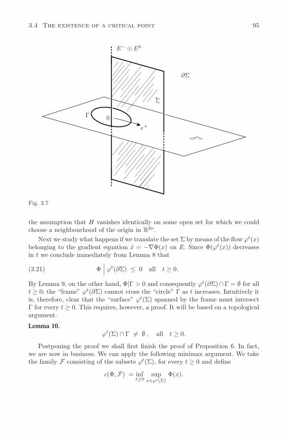
3.4 The existence of a critical point 95
E− ⊕ E0
Σ
∂Σ
Γ 0
e+
E +
Fig. 3.7
the assumption that H vanishes identically on some open set for which we couldchoose a neighbourhood of the origin in R
2n.Next we study what happens if we translate the set Σ by means of the flow ϕt(x)
belonging to the gradient equation x = −∇Φ(x) on E. Since Φ(ϕt(x)) decreasesin t we conclude immediately from Lemma 8 that
Φ∣∣∣ ϕt(∂Σ) ≤ 0 all t ≥ 0.(3.21)
By Lemma 9, on the other hand, Φ|Γ > 0 and consequently ϕt(∂Σ)∩Γ = ∅ for allt ≥ 0; the “frame” ϕt(∂Σ) cannot cross the “circle” Γ as t increases. Intuitively itis, therefore, clear that the “surface” ϕt(Σ) spanned by the frame must intersectΓ for every t ≥ 0. This requires, however, a proof. It will be based on a topologicalargument.
Lemma 10.ϕt(Σ) ∩ Γ = ∅ , all t ≥ 0.
Postponing the proof we shall first finish the proof of Proposition 6. In fact,we are now in business. We can apply the following minimax argument. We takethe family F consisting of the subsets ϕt(Σ), for every t ≥ 0 and define
c(Φ,F) = inft≥0
supx∈ϕt(Σ)
Φ(x).
96 Chapter 3 Existence of a capacity
We claim that c(Φ,F) is finite. Indeed, since ϕt(Σ) ∩ Γ = ∅ and Φ|Γ ≥ β weconclude that
β ≤ infx∈Γ
Φ(x) ≤ supx∈ϕt(Σ)
Φ(x) < ∞.
For the second estimate we have used that Φ maps, in view of Lemma 4, boundedsets into bounded sets. Therefore,
−∞ < β ≤ c(Φ,F) < ∞.
We know already that the functional Φ satisfies the P.S. condition (Lemma 6) andthat the gradient equation generates a unique global flow (Lemma 7). Moreover, bythe properties of a flow, determined by time-independent equations, the family Fis positively invariant. Consequently the Minimax Lemma guarantees that c(Φ,F)is a critical value. We deduce a point x∗ ∈ E satisfying ∇Φ(x∗) = 0 and
Φ(x∗) = c(Φ,F) ≥ β > 0,
and the Proposition is proved. It remains to prove Lemma 10.
Proof of Lemma 10. We shall use the Leray-Schauder degree. This degree extendsthe Brouwer mapping degree to infinite dimensional spaces for the restricted classof continuous mappings which are of the form id+ compact. Abbreviating the flowby ϕt(x) ≡ x · t, we wish to verify that (Σ · t)∩Γ = ∅ for all t ≥ 0. We can rewritethis by requiring
(P− + P 0)(x · t) = 0(3.22)
‖x · t‖ = α
x ∈ Σ .
Recall that, by Lemma 7, the flow has the representation x · t = et x− + x0 +e−t x+ + K(t, x), so that (3.22) becomes
0 = et x− + x0 + (P− + P 0)K(t, x)(3.23)
0 = α − ‖x · t‖
x ∈ Σ .
Multiplying the E− part by e−t one finds the equivalent equations
0 = x− + x0 + (e−t P− + P 0)K(t, x)(3.24)
0 = α − ‖x · t‖
x ∈ Σ .
3.4 The existence of a critical point 97
Since x ∈ Σ is represented by x = x− + x0 + se+, with 0 ≤ s ≤ τ , we can rewrite(3.24) as follows:
0 = x + B(t, x) and x ∈ Σ,(3.25)
where the operator B is defined by
B(t, x) = (e−t P− + P 0) K(t, x) + P+(
‖x · t‖ − α)
e+ − x
.
Abbreviating F = E− ⊕ E0 + R e+ the map B : R × F → F is continuous andmaps bounded sets into relatively compact sets. This was proved in Lemma 7.We therefore can apply the Leray-Schauder index theory. The equation (3.25)possesses, for given t ≥ 0, a solution x ∈ Σ if we can show that deg(Σ, id +B(t, ·), 0) = 0. In order to compute this degree we first observe, in view of ϕt(∂Σ)∩Γ = ∅ for t ≥ 0, that there is no solution of (3.25) on ∂Σ, i.e.,
0 ∈(id + B(t, ·)
)(∂Σ) ,
if t ≥ 0. Hence by the homotopy invariance of the degree,
deg(Σ, id + B(t, ·), 0
)= deg
(Σ, id + B(0, ·), 0
).
Since K(0, x) = 0 we find B(0, x) = P+(‖x‖−α)e+ −x. Defining the homotopy
Lµ(x) = P+
(µ‖x‖ − α) e+ − µx
for 0 ≤ µ ≤ 1,
we claim x + Lµ(x) = 0 for x ∈ ∂Σ. Indeed, if x ∈ Σ satisfies x + Lµ(x) = 0 then
x = se+ and, therefore, s((1−µ) + µ ‖e+‖
)= α. Consequently 0 < s ≤ α so that
x ∈ ∂Σ if τ > α as claimed. Therefore, by homotopy again
deg(Σ, id + B(t, ·), 0
)=
deg(Σ, id + L0, 0
)=
deg(Σ, id − αe+, 0
)=
deg(Σ, id, αe+
)= 1,
provided that αe+ ∈ Σ, which holds true for τ > α. This finishes the proof ofLemma 10 and therefore the proof of the proposition is completed.
The critical point found in the proposition is a smooth periodic solution of theHamiltonian equation z = J∇H(z) in R
2n having period 1, as we know from the“regularity” Lemma 5. This solution is the distinguished nonconstant 1-periodic
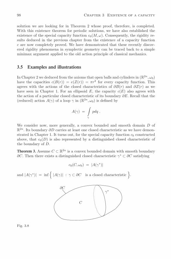
98 Chapter 3 Existence of a capacity
solution we are looking for in Theorem 2 whose proof, therefore, is completed.With this existence theorem for periodic solutions, we have also established theexistence of the special capacity function c0(M,ω). Consequently, the rigidity re-sults deduced in the previous chapter from the existence of a capacity functionc are now completely proved. We have demonstrated that these recently discov-ered rigidity phenomena in symplectic geometry can be traced back to a simpleminimax argument applied to the old action principle of classical mechanics.
3.5 Examples and illustrations
In Chapter 2 we deduced from the axioms that open balls and cylinders in (R2n, ω0)have the capacities c(B(r)) = e(Z(r)) = πr2 for every capacity function. Thisagrees with the actions of the closed characteristics of ∂B(r) and ∂Z(r) as wehave seen in Chapter 1. For an ellipsoid E, the capacity c(E) also agrees withthe action of a particular closed characteristic of its boundary ∂E. Recall that the(reduced) action A(γ) of a loop γ in (R2n, ω0) is defined by
A(γ) =∫
γ
pdq .
We consider now, more generally, a convex bounded and smooth domain D ofR
2n. Its boundary ∂D carries at least one closed characteristic as we have demon-strated in Chapter 1. It turns out, for the special capacity function c0 constructedabove, that c0(D) is also represented by a distinguished closed characteristic ofthe boundary of D.
Theorem 3. Assume C ⊂ R2n is a convex bounded domain with smooth boundary
∂C. Then there exists a distinguished closed characteristic γ∗ ⊂ ∂C satisfying
c0(C,ω0) = |A(γ∗)|
and |A(γ∗)| = inf|A(γ)| : γ ⊂ ∂C is a closed characteristic
.
∂C
C
γ∗
Fig. 3.8
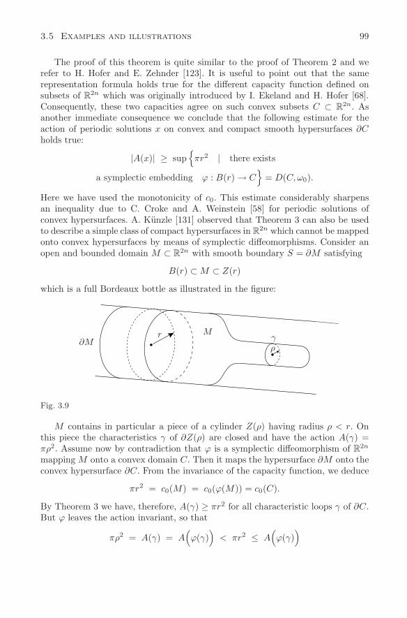
3.5 Examples and illustrations 99
The proof of this theorem is quite similar to the proof of Theorem 2 and werefer to H. Hofer and E. Zehnder [123]. It is useful to point out that the samerepresentation formula holds true for the different capacity function defined onsubsets of R
2n which was originally introduced by I. Ekeland and H. Hofer [68].Consequently, these two capacities agree on such convex subsets C ⊂ R
2n. Asanother immediate consequence we conclude that the following estimate for theaction of periodic solutions x on convex and compact smooth hypersurfaces ∂Cholds true:
|A(x)| ≥ sup
πr2 | there exists
a symplectic embedding ϕ : B(r) → C
= D(C,ω0).
Here we have used the monotonicity of c0. This estimate considerably sharpensan inequality due to C. Croke and A. Weinstein [58] for periodic solutions ofconvex hypersurfaces. A. Kunzle [131] observed that Theorem 3 can also be usedto describe a simple class of compact hypersurfaces in R
2n which cannot be mappedonto convex hypersurfaces by means of symplectic diffeomorphisms. Consider anopen and bounded domain M ⊂ R
2n with smooth boundary S = ∂M satisfying
B(r) ⊂ M ⊂ Z(r)
which is a full Bordeaux bottle as illustrated in the figure:
∂Mr M
γρ
Fig. 3.9
M contains in particular a piece of a cylinder Z(ρ) having radius ρ < r. Onthis piece the characteristics γ of ∂Z(ρ) are closed and have the action A(γ) =πρ2. Assume now by contradiction that ϕ is a symplectic diffeomorphism of R
2n
mapping M onto a convex domain C. Then it maps the hypersurface ∂M onto theconvex hypersurface ∂C. From the invariance of the capacity function, we deduce
πr2 = c0(M) = c0(ϕ(M)) = c0(C).
By Theorem 3 we have, therefore, A(γ) ≥ πr2 for all characteristic loops γ of ∂C.But ϕ leaves the action invariant, so that
πρ2 = A(γ) = A(ϕ(γ)
)< πr2 ≤ A
(ϕ(γ)
)
100 Chapter 3 Existence of a capacity
which is a contradiction. Evidently, the capacity of the above manifold M is alsorepresented by a closed characteristic on ∂M which, however, does not minimizethe action. As for general domains with smooth boundaries, it should be recalledthat it is not known whether every compact hypersurface in R
2n admits a closedcharacteristic.
In the special case of 2-dimensional compact symplectic manifolds, the regularenergy surfaces are, of course, 1-dimensional and consist of finitely many periodicorbits. This observation allowed K.F. Siburg [194] to compute the capacity c0 inthis case:
Theorem 4. (K.F. Siburg) Assume (M,ω) is a compact and connected symplecticmanifold, possibly with boundary, with dimM = 2. Then
c0(M,ω) =∣∣∣∫
M
ω∣∣∣ .
We see that c0 agrees with the total volume so that in dimension 2 this invariantclassifies symplectically diffeomorphic manifolds. This was shown in Chapter 1.
Proof. We first show that for every capacity function c
c(M,ω) ≥∣∣∣∫
M
ω∣∣∣ .
Given ε > 0, then by removing finitely many compact curves on M , we find asimply connected manifold N ⊂ M which is diffeomorphic to a closed disc D ⊂ R
2
and which satisfies ∣∣∣∫
N
ω∣∣∣ ≥
∣∣∣∫
M
ω∣∣∣− ε ,
and we can choose the radius of the disc D such that its Lebesgue measure, µ(D),agrees with the integral of ω over N . (Recall that a Riemannian surface is obtainedby a polygon in the plane by identifying suitably the edges; hence we might justremove the curves corresponding to these edges to get a disc, see W. Massey [148].)By the theorem of Dacorogna and Moser, see Chapter 1, this diffeomorphism can bechosen to be symplectic. Therefore, by the monotonicity property of the capacity
c(M,ω) ≥ c(N,ω) = c(D) = µ(D) ≥∣∣∣∫
M
ω∣∣∣− ε.
This holds true for every ε > 0 and the desired estimate is proved. It remains toprove that
c0(M,ω) ≤∣∣∣∫
M
ω∣∣∣.
3.5 Examples and illustrations 101
In view of the conformality property we may assume the integral on the right handside to be positive. Pick ε > 0 and H ∈ H(M,ω) satisfying
m(H) ≥∫
M
ω + ε.
We have to establish the existence of a nonconstant T -periodic solution of x =XH(x) on M with period 0 < T ≤ 1. Denote by R ⊂ [0,m(H)] the set of regularvalues of H. Since the set of critical levels is compact, and, in view of Sard’s the-orem, of Lebesgue measure zero, we find finitely many mutually disjoint intervalsIj = [aj , bj] ⊂ R satisfying
∑j
(bj − aj) ≥ m(H) − ε
2≥∫
M
ω +ε
2.
By definition of H(M,ω) we have H ≡ m(H) near ∂M . Therefore, if h ∈ R, thenH−1(h) consists of finitely many embedded circles S1 ⊂ M each of which carriesprecisely one (nonconstant) periodic solution γ(t, h) of XH . Choose, for every j,one of the components of H−1[aj , bj ] and call it Aj . It is simply covered by asmooth family γ(t, h) of periodic solutions having periods denoted by T (h) > 0,when h ∈ Ij . Define the diffeomorphism ϕ = ϕj
ϕ : (t, h) → γ(t, h) ∈ Aj ,
where 0 ≤ t < T (h) and aj ≤ h ≤ bj . We claim
ϕ∗ω = dt ∧ dh.
Indeed, since H(γ(t, h)) = h for all t we conclude, denoting the partial derivativeswith subscripts, ω(γt, γh) = dH(γ(t, h))(γh) = 1. Therefore, one computes forξ, η ∈ R
2, that ϕ∗ω(ξ, η) = ω(dϕ ξ, dϕη) = ω(ξ1 γt + ξ2 γh , η1 γt + η2 γh) =ξ1 η2 − ξ2 η1 = (dt ∧ dh)(ξ, η), proving the claim. Consequently,
∫
Aj
ω =∫
ϕ−1(Aj)
ϕ∗ω =
bj∫
aj
T (h) dh.
Arguing now by contradiction we assume T (h) > 1 for all h ∈ R. Then∫
M
ω ≥∑
j
∫
Aj
ω >∑
j
(bj − aj) ≥∫
M
ω +ε
2,
by the assumption on m(H). This contradiction shows that there is indeed an h ∈R and a periodic solution γ(h) lying in some Aj and having period 0 < T (h) ≤ 1.
102 Chapter 3 Existence of a capacity
In view of the definition of c0 the desired estimate follows and the proof of thetheorem is finished.
To illustrate this theorem we consider a compact 2-dimensional manifold with-out boundary. In this case the proof shows that for every H ∈ C2(M,R) satisfyingmax H −min H > |
∫ω| the Hamiltonian vector field XH admits a “fast” periodic
solution of period 0 < T ≤ 1. We would like to add another elementary observationconcerning the special case of subsets of R
2. We know from Chapter 2, that forevery capacity function, c(D) = area(D) for a bounded connected subset D of R
2
having smooth boundary. Since the special capacity c0 has the additional propertyof inner regularity we can easily extend this statement to open subsets of R
2.
Proposition 7. If Ω ⊂ R2 is an open bounded and path connected set, then
c0(Ω, ω0) = area(Ω).
Proof. Exhaust Ω =⋃
Kj , j ≥ 1 by compact sets Kj ⊂Kj+1 and define smooth
functions βj : Ω R by setting βj(x) = 0 if x ∈ Kj and βj(x) = 1 if x ∈ Ω\Kj+1.Define β ∈ C∞(Ω) by
β(x) =∑j≥1
βj(x) , x ∈ Ω.
Then β(x) → +∞ as x → R2\Ω. Now take a sequence bn → ∞ of regular values
of β and consider the compact symplectic manifolds Dj = β−1(−∞, bj ] havingsmooth boundaries. Then Ω = ∪Dj, j ≥ 1. Since c0 has the property of innerregularity we conclude c0(Ω) = lim c0(Dj), as j → ∞. From the regularity ofthe Lebesgue measure we find, on the other hand, area (Ω) = lim area (Dj)as j → ∞. Since we already know that c0(Dj) = area (Dj), the proposition isproved.
Although the invariant c0 is defined by means of special periodic solutions, itis not at all surprising that in the 2-dimensional case it is intimately related to thearea, since the symplectic form is the area form. In higher dimensions the capacityc0 is, in contrast, not yet understood. It turns out that it is extremely difficult tocompute this capacity. But some examples are known which are mentioned next.
Theorem 5. Consider (CPn, ω) with the standard symplectic structure related tothe Fubini-Study metric. Then
c0 (CPn, ω) = π.
This result is due to H. Hofer and C. Viterbo [122]. We do not give a proofhere and remark that the proof analyzes the structure of the holomorphic spheresin CPn and is based on a Fredholm theory for first order elliptic systems. Nowassume that (M,ω) is any compact symplectic manifold without boundary, anddenote by π2(M) the homotopy classes of maps u : S2 → M . Then there is a mapπ2(M) → R given by
u → 〈ω, u〉 =∫
S2
u∗ω ∈ R.
3.5 Examples and illustrations 103
Define α∗(M) ∈ R ∪ ∞ by
α∗(M) = inf〈ω, u〉
∣∣∣u ∈ π2(M) and 〈ω, u〉 > 0.
Moreover, if π2(M) = 0, we set α∗ = ∞. Then the following result due to A. Floer– H. Hofer – C. Viterbo[88] and R. Ma [146] holds true.
Theorem 6. Consider the symplectic manifold (M × R2n, ω ⊕ ω0) with n ≥ 1 and
assume α∗ = α∗(M) > 0 or α∗ = ∞. Then
c0
(M × B(r)
)= c0
(M × Z(r)
)= πr2 ,
provided πr2 < α∗.The case of the symplectic torus T 2n will be discussed in the next chapter.Incidentally, by restricting the class of Hamiltonian functions admitted in
the definition of c0(M,ω), one finds different capacity functions. For example,if H(M,ω) = H ∈ H(M,ω)| support of ∇H is contractible in M and corre-spondingly Ha(M,ω) = Ha(M,ω) ∩ H(M,ω), then we can define
c0 (M,ω) = sup
m(H)∣∣∣ H ∈ Ha(M,ω)
.
Our proof shows that c0 is a capacity function; the related periodic solutions areall contractible. It clearly satisfies
D(M,ω) ≤ c0(M,ω) ≤ c0(M,ω)
where D(M,ω) is the Gromov-width introduced in Chapter 1.
Chapter 4
Existence of closed characteristics
In the previous chapter, the dynamical approach to the symplectic invariants led tothe special capacity function c0. Its construction was based on a variational prin-ciple for periodic solutions of certain Hamiltonian systems. The period of theseperiodic solutions was prescribed. In this chapter we shall deduce from this sym-plectic invariant the existence of periodic solutions on prescribed energy surfaces.If we neglect the parametrization of such solutions the aim is to find closed charac-teristics of a distinguished line bundle over a hypersurface in a symplectic manifold.It is determined by the symplectic structure, as explained in the introduction. Avery special symplectic structure on the torus will lead us to M. Herman’s coun-terexample to the closing lemma in the smooth category.
4.1 Periodic solutions on energy surfaces
The flow ϕt of a Hamiltonian vector field
x = XH(x) , x ∈ M(4.1)
on a symplectic manifold (M,ω) leaves the level sets of the smooth function H onM invariant, i.e., H(ϕt(x)) = H(x) as long as t is defined. Fixing a value of thisenergy function which we can assume to be E = 1, we shall require the subset
S =
x ∈ M∣∣∣ H(x) = 1
(4.2)
to be compact and a regular, i.e.,
dH(x) = 0 for x ∈ S.(4.3)
Thus S ⊂ M is a smooth and compact submanifold of codimension 1 whose tangentspace at x ∈ S is given by
TxS =
ξ ∈ TxM∣∣∣ dH(x)ξ = 0
.(4.4)
By the definition of a Hamiltonian vector field we have XH(x) ∈ TxS so that XH isa nonvanishing vector field on S whose flow exists for all times since S is compact.Our aim is to find a periodic solution for XH on the energy surface S. This is aqualitative existence problem described in the introduction.
In order to illustrate the method employed we start with a preliminary result.The trick is to thicken the given energy surface S and to consider a 1-parameter
H. Hofer and E. Zehnder, Symplectic Invariants and Hamiltonian Dynamics, 105Modern Birkhäuser Classics, DOI 10.1007/978-3-0348-0104-1_4, © Springer Basel AG 2011
106 Chapter 4 Existence of closed characteristics
family of surfaces parameterized by the energy. Since S is compact and regularthere is an open and bounded neighborhood U of S which is filled with compactand regular energy surfaces having energy values near E = 1:
U =⋃λ∈I
Sλ,(4.5)
where I is an open interval around λ = 1 and where Sλ = x ∈ U |H(x) = λis diffeomorphic to the given surface S, which corresponds to the parameter valueλ = 1. Indeed, take any Riemannian metric on M , then the gradient of H withrespect to this metric does not vanish, ∇H = 0, in a neighborhood of S, in viewof (4.3). We can, therefore, define the modified gradient vector field
x =∇H(x)
|∇H(x)|2
near S, which is transversal to S. Its flow ψt satisfies
H(ψt(x)
)= 1 + t
for x ∈ S and, therefore, defines a diffeomorphism (x, t) → ψt(x) from S × (−ε, ε)onto an open neighborhood U of S as claimed.
Theorem 1. (Hofer-Zehnder) Let S be a compact and regular energy surface for theHamiltonian vector field XH on (M,ω). Assume there is an open neighborhoodU of S having bounded capacity: c0(U, ω) < ∞. Then there exists a sequenceλj → 1 of energy values, such that XH possesses a periodic solution on everyenergy surface Sλj
.
Actually, the proof establishes more solutions:
Corollary. There is a dense subset Σ ⊂ I such that for λ ∈ Σ the energy surfaceSλ has a periodic solution of XH , provided c0(U, ω) < ∞.
It should be emphasized that there are no assumptions required for the givenregular and compact energy surface S other than that a bounded open neighbor-hood must have finite capacity. For example, in the special case of the standardsymplectic manifold (R2n, ω0) a bounded set U is contained in a large ball B(R)and, consequently, by the monotonicity of the capacity, always has finite capacity.Hence every compact regular energy surface S ⊂ R
2n gives rise to an abundanceof periodic solutions for the Hamiltonian vector fields XH having energies near theprescribed energy.
Proof. The statement is an immediate consequence of the definition of the spe-cial capacity c0 if we recall from the introduction that we have the freedom tochoose a convenient Hamiltonian function representing the energy surfaces. Weshall construct an auxiliary Hamiltonian function F on U which is constant on
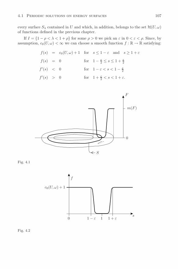
4.1 Periodic solutions on energy surfaces 107
every surface Sλ contained in U and which, in addition, belongs to the set H(U, ω)of functions defined in the previous chapter.
If I = 1− ρ < λ < 1 + ρ for some ρ > 0 we pick an ε in 0 < ε < ρ. Since, byassumption, c0(U, ω) < ∞ we can choose a smooth function f : R → R satisfying:
f(s) = c0(U, ω) + 1 for s ≤ 1 − ε and s ≥ 1 + ε
f(s) = 0 for 1 − ε2 ≤ s ≤ 1 + ε
2
f ′(s) < 0 for 1 − ε < s < 1 − ε2
f ′(s) > 0 for 1 + ε2 < s < 1 + ε.
F
m(F )
0U
S
Fig. 4.1
f
c0(U, ω) + 1
0 11 − ε 1 + εs
Fig. 4.2
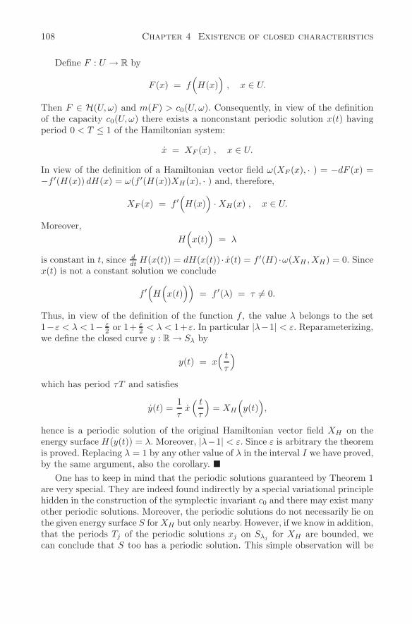
108 Chapter 4 Existence of closed characteristics
Define F : U → R by
F (x) = f(H(x)
), x ∈ U.
Then F ∈ H(U, ω) and m(F ) > c0(U, ω). Consequently, in view of the definitionof the capacity c0(U, ω) there exists a nonconstant periodic solution x(t) havingperiod 0 < T ≤ 1 of the Hamiltonian system:
x = XF (x) , x ∈ U.
In view of the definition of a Hamiltonian vector field ω(XF (x), · ) = −dF (x) =−f ′(H(x)) dH(x) = ω(f ′(H(x))XH(x), · ) and, therefore,
XF (x) = f ′(H(x)
)· XH(x) , x ∈ U.
Moreover,H(x(t)
)= λ
is constant in t, since ddt H(x(t)) = dH(x(t)) · x(t) = f ′(H) ·ω(XH , XH) = 0. Since
x(t) is not a constant solution we conclude
f ′(H(x(t)
))= f ′(λ) = τ = 0.
Thus, in view of the definition of the function f , the value λ belongs to the set1−ε < λ < 1− ε
2 or 1+ ε2 < λ < 1+ε. In particular |λ−1| < ε. Reparameterizing,
we define the closed curve y : R → Sλ by
y(t) = x( t
τ
)
which has period τT and satisfies
y(t) =1τ
x( t
τ
)= XH
(y(t)
),
hence is a periodic solution of the original Hamiltonian vector field XH on theenergy surface H(y(t)) = λ. Moreover, |λ−1| < ε. Since ε is arbitrary the theoremis proved. Replacing λ = 1 by any other value of λ in the interval I we have proved,by the same argument, also the corollary.
One has to keep in mind that the periodic solutions guaranteed by Theorem 1are very special. They are indeed found indirectly by a special variational principlehidden in the construction of the symplectic invariant c0 and there may exist manyother periodic solutions. Moreover, the periodic solutions do not necessarily lie onthe given energy surface S for XH but only nearby. However, if we know in addition,that the periods Tj of the periodic solutions xj on Sλj
for XH are bounded, wecan conclude that S too has a periodic solution. This simple observation will be
4.1 Periodic solutions on energy surfaces 109
very useful later on. To be precise we choose a Riemannian metric g on M andabbreviate g(x)(ξ, η) = 〈ξ, η〉 and g(x)〈ξ, ξ〉 = |ξ|2. If x(t) is a periodic solution ofperiod T we can introduce its length by
l(x) =
T∫
0
|x(t)| dt.
Possibly after shrinking the open neighborhood U , we may assume
C−1 ≤ |XH(x)| ≤ C , x ∈ U
for a constant C > 0. Since the xj(t) solve the Hamiltonian equations xj(t) =XH(xj(t)) we conclude
C−1 · Tj ≤ l(xj) ≤ C · Tj .
Proposition 1. Let λj → 1 and assume that the periods Tj (or equivalently thelengths l(xj)) of the periodic solutions xj(t) on Sλj
are bounded. Then S = S1
possesses a periodic solution of XH .
Proof. Normalizing the periods to 1 we define yj(t) = xj(Tj · t) for 0 ≤ t ≤ 1, sothat
yj(t) = Tj XH
(yj(t)
)
and H(yj(t)) = λj . Since, by assumption, the right hand side is bounded, wefind by means of the Arzela-Ascoli theorem a subsequence such that Tj → T andyj → y with convergence, at first in C0, and, by making use of the equation, inC∞. The function y : [0, 1] → U is periodic with period 1, satisfies H(y(t)) = 1,and
y(t) = TXH
(y(t)
),
and is thus the desired periodic solution if T = 0. Arguing by contradiction, we as-sume T = 0. Then yj → y∗ shrinks to a point y∗ and XH(y(t)) → XH(y∗) = V .Since the energy surface S is regular, V = 0. We can estimate in local coordinatesnear the point y∗;
〈XH(yj), V 〉 ≥ (1 − ε) |V |2
for some small ε > 0 and all j sufficiently large, so that
T−1j 〈yj(t), V 〉 ≥ (1 − ε) |V |2.
Integrating over the period we conclude V = 0 contradicting V = 0 and provingthe proposition.
Having established the existence of periodic solutions of a Hamiltonian vectorfield XH , it is useful to remember that, in general, a periodic solution belongs to a
110 Chapter 4 Existence of closed characteristics
whole family of periodic solutions parameterized by the energy. This will be provedby the so-called Poincare continuation method. This local technique is based on theimplicit function theorem and requires some knowledge of the Floquet multipliersof a given reference solution.
Consider a periodic solution x(t) = x(t, E∗) of XH having energy E∗ = H(x(t))and period T = T ∗. Since the vector field XH is time independent one of theFloquet multipliers of x(t) must be equal to 1. Indeed, abbreviating x = x(0) wecan differentiate the flow ϕt ϕs(x) = ϕs ϕt(x) in s at s = 0 and obtain
dϕt(x) XH(x) = XH
(ϕt(x)
)
for all t. If t = T is the period and hence ϕT (x) = x we obtain
dϕT (x) XH (x) = XH (x) ∈ TxM.
By definition, the eigenvalues of the linear map dϕT (x) : TxM → TxM are theFloquet multipliers of the periodic solution x(t) and we have just verified that 1is always a Floquet multiplier. But since dϕT (x) is a symplectic linear map, theeigenvalue 1 has necessarily even multiplicity, so that x(t) possesses always at leasttwo-Floquet multipliers equal to 1. Actually we shall verify this during the proofof the following proposition which was known to H. Poincare.
Proposition 2. Assume a periodic solution x(t, E∗) of XH on M having energyE∗ = H(x(t, E∗)) and period T ∗ has exactly two Floquet multipliers equal to1. Then there exists a unique and smooth 1-parameter family x(t, E) of periodicsolutions with periods T (E) close to T ∗ and lying on the energy surfaces
H(x(t, E)
)= E
for |E − E∗| sufficiently small. Moreover, T (E) → T (E∗) as E → E∗.Postponing the proof we observe that the reference solution x(t, E∗) is not
isolated in M as a periodic solution. The periodic solutions x(t, E) correspond todifferent values of E and it will turn out in the proof that, on the fixed energysurface E, this solution is isolated among those periodic solutions having peri-ods close to T . Geometrically, the periodic solutions x(t, E) fill out an embeddedcylinder in M as illustrated in the following figure 4.3.
Proof of Proposition 2. It is useful to recall the construction of a transversal sectionmap belonging to a periodic solution. Assume x(t) to be a nonconstant periodicsolution of a vector field X on M and denote by T > 0 its period. Then, we canintersect x(t) at the point p = x(0) with a (2n − 1) dimensional hypersurface,i.e., a local submanifold Σ ⊂ M with codim Σ = 1 to which the vector field X isnowhere tangential. This means that TxΣ and X(x) span the tangent space TxMfor every x ∈ Σ near p:
TxM = TxΣ ⊕ 〈X(x)〉 , x ∈ Σ.
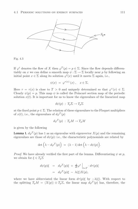
4.1 Periodic solutions on energy surfaces 111
SE*
Fig. 4.3
If ϕt denotes the flow of X then ϕT (p) = p ∈ Σ. Since the flow depends differen-tiably on x we can define a smooth map ψ : Σ → Σ locally near p by following aninitial point x ∈ Σ along its solution ϕt(x) until it meets Σ again, i.e.,
ψ(x) = ϕτ(x) (x) , x ∈ Σ.
Here τ = τ(x) is close to T > 0 and uniquely determined so that ϕτ (x) ∈ Σ.Clearly ψ(p) = p. This map ψ is called the Poincare section map of the periodicsolution x(t). It is important for us to know the eigenvalues of the linearized map
dψ(p) : TpΣ → TpΣ
at the fixed point p ∈ Σ. The relation of these eigenvalues to the Floquet multipliersof x(t), i.e., the eigenvalues of dϕT (p)
dϕT (p) : TpM → TpM
is given by the following
Lemma 1. dϕT (p) has 1 as an eigenvalue with eigenvector X(p) and the remainingeigenvalues are those of dψ(p): i.e., the characteristic polynomials are related by
det(λ − dϕT (p)
)= (λ − 1) det
(λ − dψ(p)
).
Proof. We have already verified the first part of the lemma. Differentiating ψ at p,we obtain for ξ ∈ TpΣ
dψ(p)ξ = dϕT (p)ξ + ddtϕ
t∣∣∣t=T
· dτ(p)ξ
= dϕT (p)ξ − λ(ξ)X(p),
where we have abbreviated the linear form dτ(p)ξ by −λ(ξ). With respect tothe splitting TpM = 〈X(p)〉 ⊕ TpΣ, the linear map dϕT (p) has, therefore, the
112 Chapter 4 Existence of closed characteristics
representation
dϕT (p) =
1 λ
0 dψ(p)
,
from which the lemma follows immediately. Evidently the fixed points of ψ near p are the initial conditions of all the
periodic solutions near the reference solutions x(t) which have periods near T .We shall use this observation in order to prove Proposition 2. Let x(t) be theperiodic solution of the proposition. Then H(x(t)) = E∗ and dH(x) = 0 for xnear x(t). Moreover, dH(XH) = 0. We can, therefore, introduce near p = x(0)convenient local coordinates (x1, . . . , x2n) ∈ R
2n such that p corresponds to x∗ =(E∗, 0, . . . , 0) and such that H(x1, . . . , x2n) = x1 and moreover, such that x2n = 0is a local transversal section Σ. In view of H(ϕt(x)) = H(x) the section map ψ is,in these coordinates expressed by
ψ :
(x′
x′′
)−→
(ψ′(x′, x′′) = x′
ψ′′(x′, x′′)
).
where the coordinates (x′, x′′) ∈ Σ stand for x′ = x1 and x′′ = (x2, . . . , x2n−1).The aim is to find the fixed points of ψ near x∗. In order to do this we only haveto solve the equation
ψ′′(x′, x′′) = x′′,
since the first equation ψ′(x′, x′′) = x′ is automatically satisfied. Since, by as-sumption, ψ(x∗) = x∗ is a reference solution, we can apply the implicit functiontheorem, observing that in our coordinates the linearized map is expressed by
dψ(x∗) =
1 0
∗ ∂∂x′′ ψ′′(x∗)
.
Recalling the assumption of Proposition 2 and Lemma 1, the matrix
∂
∂x′′ ψ′′(x∗) − 1l2n−2
is nonsingular. Therefore, there exists a unique map x′ → x′′ = a(x′) solvingthe equation ψ′′(x′, a(x′)) = a(x′). Thus x′ = E and x′′ = a(E) are the initialconditions on Σ of the desired periodic solutions satisfying Proposition 2.
One is tempted to apply Proposition 2 to the periodic solutions on Sλjguar-
anteed by Theorem 1 in order to establish the existence of a periodic solutionon the given energy surface S as λj → 0. But unfortunately nothing can be saidabout the Floquet multipliers of these solutions. In addition, Proposition 2 is ofa local nature: globally the cylinder of periodic solutions may eventually becometangential to an energy surface. This situation has been studied by C. Robinsonin [183], 1970.
4.2 The characteristic line bundle of a hypersurface 113
4.2 The characteristic line bundle of a hypersurface
The search for periodic orbits of a Hamiltonian vector field lying on a prescribedenergy surface S is independent of the choice of the Hamiltonian representing S:it only depends on the submanifold S and the symplectic structure ω. Indeed, asexplained in Chapter 1, this dynamical problem can be described geometrically.We consider a submanifold S ⊂ M of codimension 1, i.e., a hypersurface of thesymplectic manifold (M,ω). Then the symplectic structure ω and S determine adistinguished line bunde LS ⊂ TS, as follows. If x ∈ S, then restriction of the2-form ω to the odd-dimensional subspace TxS ⊂ TxM is necessarily degenerate.The kernel of this restriction if of dimension 1, because ω is nondegenerate onTxM , and hence defines a line bundle, LS ⊂ TS,
LS = (x, ξ) ∈ TxS |ωx(ξ, η) = 0 for all η ∈ TxS .
This line bundle gives the direction of every Hamiltonian vector field having S asa regular energy surface.
Proposition 3. Assume the smooth function H represents S as S = x|H(x) =const and satisfies dH = 0 on S. Then
XH(x) ∈ LS(x) for all x ∈ S .
Proof. Since the tangent space is given by TxS = ξ ∈ TxM |dH(x)ξ = 0 we haveω(XH(x), ξ) = −dH(x)ξ = 0 for all ξ ∈ TxS.
Notation. The bundle LS is called the characteristic line bundle of the hypersurfaceS. A closed characteristic of S, or a periodic Hamiltonian orbit of S, is an embeddedcircle P ⊂ S satisfying
TP = LS |P.
In the following we shall denote the set of closed characteristics of S by
P(S).
It agrees with the set of unparameterized periodic solutions of every Hamiltonianvector field XH on S having S as a regular energy surface.
Assume now that LS → S is orientable, i.e., the bundle possesses a nonvanish-ing section. We shall show that there exists a Hamiltonian function H : U → R
defined on a neighborhood of S and representing S = H−1(0) as a regular energysurface. We make use of an almost complex structure on M compatible with ω,i.e., a smooth family of linear maps J(x) ∈ L(TxM), x ∈ M , satisfying J2 = −1land
ω(x)(ξ, J(x)η
)= g(x) (ξ, η)
114 Chapter 4 Existence of closed characteristics
for all ξ, η ∈ TxM , with a Riemannian metric g. If NS → S is the normal bundleof S whose fibre at x ∈ S is defined by
NS(x) =η ∈ TxM
∣∣∣ g(x)(η, ξ) = 0 for all ξ ∈ TxS
,
we have the bundle isomorphism
LS → NS : (x, ξ) →(x, J(x)ξ
).
This map is indeed well-defined and injective on each fibre: if ω(ξ, η) = 0 forall η ∈ TxS then g(η, Jξ) = ω(η, J2ξ) = −ω(η, ξ) = 0. The normal bundle NS isorientable since LS is orientable. Therefore, NS and S×R are isomorphic as vectorbundles. Taking a nonvanishing section σ of NS, so that 0 = σ(x) ∈ NS(x) ⊂ TxMwe can define the map
ψ : S × (−ε, ε) → U ⊂ M
by means of the exponential map (x, t) → expx(tσ(x)). It is a diffeomorphism ontoan open neighborhood U of S if S is compact and ε sufficiently small. If
F : S × (−ε, ε) → R
is the smooth function F (x, t) = t, then the composition H = F ψ−1 : U → R isthe desired Hamiltonian; it satisfies S = H−1(0) and dH = 0 as claimed.
Definition. Let S be a compact hypersurface in (M,ω). A parameterized family ofhypersurfaces modelled on S is a diffeomorphism
ψ : S × I → U ⊂ M,
I being an open interval containing 0, onto a bounded neighborhood U of S sat-isfying
ψ(x, 0) = x for x ∈ S.
We shall abbreviate in the following Sε = ψ(S×ε) and later on we often simplywrite (Sε) instead of ψ.
We remark that the following statements are equivalent: (i) The line bundleLS → S is orientable. (ii) The normal bundle NS → S is orientable. (iii) S isorientable. (iv) There exists a parameterized family of hypersurfaces modelledon S. (v) There exists a smooth function H ∈ C∞(U, R) defined on an openneighborhood U of S representing S = x ∈ U |H(x) = const. and satisfyingdH = 0. Using these concepts we can reformulate Theorem 1 of the previoussection as follows:
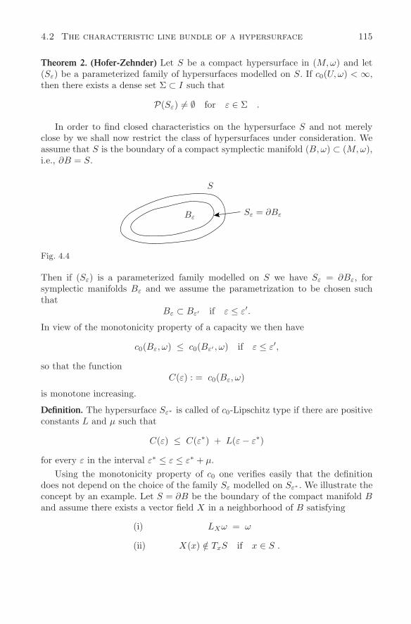
4.2 The characteristic line bundle of a hypersurface 115
Theorem 2. (Hofer-Zehnder) Let S be a compact hypersurface in (M,ω) and let(Sε) be a parameterized family of hypersurfaces modelled on S. If c0(U, ω) < ∞,then there exists a dense set Σ ⊂ I such that
P(Sε) = ∅ for ε ∈ Σ .
In order to find closed characteristics on the hypersurface S and not merelyclose by we shall now restrict the class of hypersurfaces under consideration. Weassume that S is the boundary of a compact symplectic manifold (B,ω) ⊂ (M,ω),i.e., ∂B = S.
S
BεSε = ∂Bε
Fig. 4.4
Then if (Sε) is a parameterized family modelled on S we have Sε = ∂Bε, forsymplectic manifolds Bε and we assume the parametrization to be chosen suchthat
Bε ⊂ Bε′ if ε ≤ ε′.
In view of the monotonicity property of a capacity we then have
c0(Bε, ω) ≤ c0(Bε′ , ω) if ε ≤ ε′,
so that the functionC(ε) : = c0(Bε, ω)
is monotone increasing.
Definition. The hypersurface Sε∗ is called of c0-Lipschitz type if there are positiveconstants L and µ such that
C(ε) ≤ C(ε∗) + L(ε − ε∗)
for every ε in the interval ε∗ ≤ ε ≤ ε∗ + µ.Using the monotonicity property of c0 one verifies easily that the definition
does not depend on the choice of the family Sε modelled on Sε∗ . We illustrate theconcept by an example. Let S = ∂B be the boundary of the compact manifold Band assume there exists a vector field X in a neighborhood of B satisfying
(i) LXω = ω
(ii) X(x) /∈ TxS if x ∈ S .
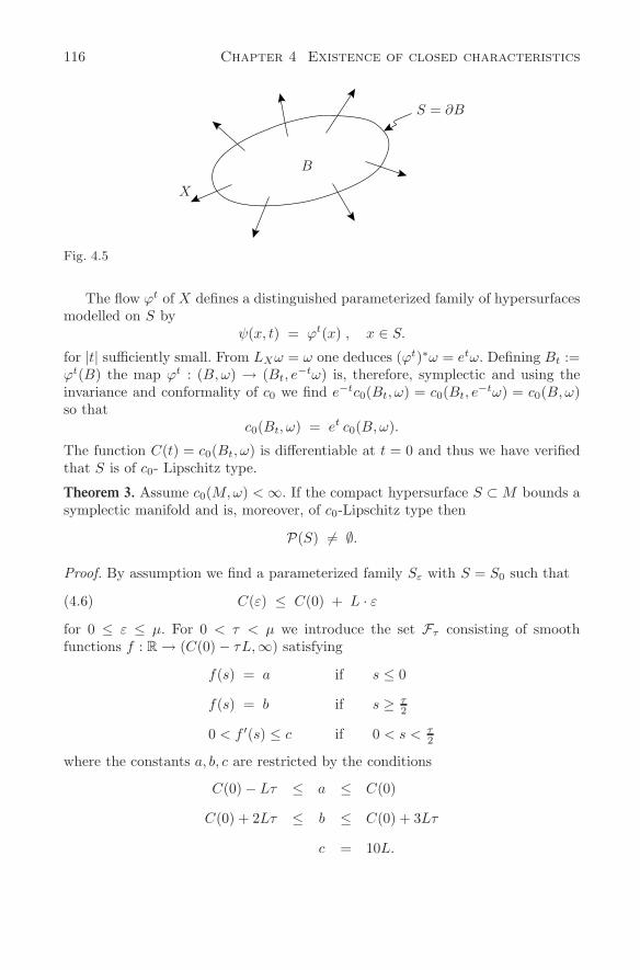
116 Chapter 4 Existence of closed characteristics
X
B
S = ∂B
Fig. 4.5
The flow ϕt of X defines a distinguished parameterized family of hypersurfacesmodelled on S by
ψ(x, t) = ϕt(x) , x ∈ S.
for |t| sufficiently small. From LXω = ω one deduces (ϕt)∗ω = etω. Defining Bt :=ϕt(B) the map ϕt : (B,ω) → (Bt, e
−tω) is, therefore, symplectic and using theinvariance and conformality of c0 we find e−tc0(Bt, ω) = c0(Bt, e
−tω) = c0(B,ω)so that
c0(Bt, ω) = et c0(B,ω).
The function C(t) = c0(Bt, ω) is differentiable at t = 0 and thus we have verifiedthat S is of c0- Lipschitz type.
Theorem 3. Assume c0(M,ω) < ∞. If the compact hypersurface S ⊂ M bounds asymplectic manifold and is, moreover, of c0-Lipschitz type then
P(S) = ∅.
Proof. By assumption we find a parameterized family Sε with S = S0 such that
C(ε) ≤ C(0) + L · ε(4.6)
for 0 ≤ ε ≤ µ. For 0 < τ < µ we introduce the set Fτ consisting of smoothfunctions f : R → (C(0) − τL,∞) satisfying
f(s) = a if s ≤ 0
f(s) = b if s ≥ τ2
0 < f ′(s) ≤ c if 0 < s < τ2
where the constants a, b, c are restricted by the conditions
C(0) − Lτ ≤ a ≤ C(0)
C(0) + 2Lτ ≤ b ≤ C(0) + 3Lτ
c = 10L.
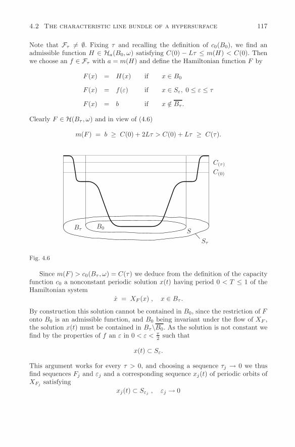
4.2 The characteristic line bundle of a hypersurface 117
Note that Fτ = ∅. Fixing τ and recalling the definition of c0(B0), we find anadmissible function H ∈ Ha(B0, ω) satisfying C(0) − Lτ ≤ m(H) < C(0). Thenwe choose an f ∈ Fτ with a = m(H) and define the Hamiltonian function F by
F (x) = H(x) if x ∈ B0
F (x) = f(ε) if x ∈ Sε, 0 ≤ ε ≤ τ
F (x) = b if x /∈ Bτ .
Clearly F ∈ H(Bτ , ω) and in view of (4.6)
m(F ) = b ≥ C(0) + 2Lτ > C(0) + Lτ ≥ C(τ).
C(τ)
C(0)
Bτ B0S
Sτ
Fig. 4.6
Since m(F ) > c0(Bτ , ω) = C(τ) we deduce from the definition of the capacityfunction c0 a nonconstant periodic solution x(t) having period 0 < T ≤ 1 of theHamiltonian system
x = XF (x) , x ∈ Bτ .
By construction this solution cannot be contained in B0, since the restriction of Fonto B0 is an admissible function, and B0 being invariant under the flow of XF ,the solution x(t) must be contained in Bτ\B0. As the solution is not constant wefind by the properties of f an ε in 0 < ε < τ
2 such that
x(t) ⊂ Sε.
This argument works for every τ > 0, and choosing a sequence τj → 0 we thusfind sequences Fj and εj and a corresponding sequence xj(t) of periodic orbits ofXFj
satisfyingxj(t) ⊂ Sεj
, εj → 0
118 Chapter 4 Existence of closed characteristics
and having periods 0 < Tj ≤ 1. These solutions satisfy, in addition, some estimatesindependent of j. Define on
U =⋃ε∈I
Sε
a fixed Hamiltonian function K having the hypersurfaces Sε as regular energysurfaces by setting
K(x) = ε if x ∈ Sε.
If x ∈ Sε and 0 ≤ ε ≤ µ then for every τj we have Fj(x) = fj(K(x)) and,therefore, XF (x) = f ′(K(x)) · XK(x) where we did not indicate the dependenceof the functions f and F on j. By construction, the periodic functions solve theequations
xj(t) = f ′(εj)XK
(xj(t)
)
xj(0) = xj(Tj)
and 0 < Tj ≤ 1. Reparameterizing, the functions
yj(t) = xj
(t
f ′(εj)
)
solve the Hamiltonian equations
yj(t) = XK(yj) and K(yj(t)
)= εj .
The crucial observation now is that the periods of yj are given by f ′(εj) · Tj
and hence, in view of f ′(εj) ≤ 10M , the periods are bounded. By Proposition1 we, therefore, conclude that there exists a periodic solution x(t) of XK on theenergy surface K(x) = 0 which is the hypersurface S = S0. This periodic solutionparameterizes the desired closed characteristic on S.
Recall now that the function C(ε) = c0(Bε, ω) defined above is monotone. Bya theorem due to Lebesgue it is, therefore, differentiable almost everywhere andthus Lipschitz continuous almost everywhere and we deduce from Theorem 3
Theorem 4. Assume the hypersurface S ⊂ (M,ω) bounds a compact symplecticmanifold. If (Sε) with ε ∈ I is a parameterized family of hypersurfaces modelledon S, then (m denoting Lebesgue measure)
m
ε ∈ I∣∣∣ P (Sε) = ∅
= m(I),
provided c0(M,ω) < ∞.A compact and connected hypersurface S ⊂ R
2n separates the space into abounded and an unbounded component. (Indeed, every compact smooth hyper-surface M ⊂ R
m is orientable; the statement follows from the Jordan-Brouwerseparation theorem, we refer to E. Lima [142] for a short differential geometricproof in the smooth case.)We, therefore, conclude for the special case of hypersur-faces in the standard symplectic manifold (R2n, ω0) the
4.3 Hypersurfaces of contact type, the Weinstein conjecture 119
Corollary. For every compact hypersurface S ⊂ (R2n, ω0) and every parameterizedfamily (Sε), ε ∈ I, of hypersurfaces modelled on S
m
ε ∈ I∣∣∣ P(Sε) = ∅
= m(I).
This result was first proved by M. Struwe in [207] who cleverly modified theproof by H. Hofer and E. Zehnder in [123] of the weaker statement that P(Sε) = ∅for a dense set of ε in I. As an illustration we take a smooth function H ∈ C∞
c (R2n),i.e., having compact support. Then the set of critical levels is compact in R and,moreover, by Sard’s theorem of measure zero. Consequently, for almost every h in
min H < h < max H
there exists a nonconstant periodic solution xh(t) of the Hamiltonian vector fieldXH having energy H(xh(t)) = h. This is a local analogue to a recent result due toC. Viterbo [218] for mappings instead of vector fields. It states that a symplecticdiffeomorphism ϕ of (R2n, ω0) which is the identity map outside a compact setK ⊂ R
2n possesses infinitely many periodic orbits contained in K. We shouldmention that C. Viterbo also deduced his result from the existence of a symplecticinvariant for subsets in (R2n, ω0) whose relation to the capacity c0 is so far notunderstood.
4.3 Hypersurfaces of contact type, the Weinstein conjecture
We next single out another symplectic property of a hypersurface which guaranteesthe existence of a closed characteristic. Prompted by the first global results forconvex and star-like energy surfaces in R
2n, A. Weinstein introduced in [226] thefollowing concept:
Definition. A compact and orientable hypersurface S ⊂ M in the symplectic man-ifold (M,ω) is called of contact type if there exists a 1-form α on S satisfying
(i) dα = j∗ω
(ii) α(ξ) = 0 for 0 = ξ ∈ LS ,
where j : S → M is the inclusion map and LS is the canonical line bundle of S.
Since ξ ∈ LS is in the kernel of ω|S and α(ξ) = 0, the kernel of α, givenby kerα(x) = η ∈ TxS |αx(η) = 0, is a (2n − 2)-dimensional subspace of TxSon which the 2-form ω, and hence also dα is nondegenerate. Consequently, α ∧(dα)n−1 is a volume form on S. Geometrically the 1-form α defines a smoothfield of hyperplanes on S which is an example of a contact structure on the odd-dimensional manifold S.
120 Chapter 4 Existence of closed characteristics
A. Weinstein conjecture (1978): A hypersurface S of contact type and satisfyingH1(S) = 0 carries a closed characteristic.
We shall verify the conjecture without the topological assumption H1(S) = 0but under the symplectic assumption that S has a neighborhood U ⊂ M of finitecapacity: c0(U, ω) < ∞. We first reformulate the concept of contact type followingA. Weinstein [226].
Proposition 4. A compact hypersurface S ⊂ M is of contact type if and only ifthere exists a vector field X, defined on a neighborhood U of S, satisfying
(i) LXω = ω on U .
(ii) X(x) /∈ TxS if x ∈ S .
i.e., X is transversal to S.In order to prove the proposition we start with a Poincare-type lemma.
Lemma 2. Let π : E → N be a vector bundle and let α be a closed k-form on Esatisfying j∗α = 0, where the inclusion map j : N → E is the zero section of thebundle. Then there exists a (k − 1)-form β on E satisfying
α = dβ and β|N = 0.
Proof. Using the linear structure of the fibers we can define, for t > 0, the con-traction maps ϕt : E → E along the fibers by multiplication: ϕt(x) = t · x.With Xt we denote the time-dependent vector field on E generated by the fam-ily of diffeomorphisms as usual by d
dtϕt(x) = Xt(ϕt(x)) if t > 0. If we define
X1(x) = ddt ϕt(x)|t=1 ∈ TxE we have the representation Xt(x) = 1
t X1(x). More-over, Xt(x) = 0 if x ∈ N . Using dα = 0 we find by Cartan’s formula
d
dt(ϕt)∗ α = (ϕt)∗ LXt
α = d(ϕt)∗iXt
α
,
where(ϕt)∗ iXt
α(x) = α(t · x)(1
tdϕtX1(x), dϕt ·
).
Because limt→0
(ϕt)∗α = π∗j∗α = 0 and ϕ1(x) = x we conclude that
α = (ϕ1)∗α − limt→0
(ϕt)∗α
= limt→0
1∫t
ddt
(ϕt)∗α dt
= d1∫0
((ϕt)∗iXt
α)
dt = dβ
for a smooth (k − 1)-form β on E. If x ∈ N , then Xt(x) = 0 and hence iXtα = 0
so that β(x) = 0. This finishes the proof of the lemma. We shall use the lemma to extend the 1-form α on S to an open neighborhood
of S.
4.3 Hypersurfaces of contact type, the Weinstein conjecture 121
Lemma 3. If S ⊂ (M,ω) is of contact type then there exists a 1-form τ on aneighborhood U of S satisfying
(i) dτ = ω on U
(ii) j∗τ = α on S
where j : S → U is the inclusion mapping.
Proof. Since S is compact and oriented there exists a diffeomorphism ψ : S ×(−1, 1) → U onto an open neighborhood U of S satisfying ψ(x, 0) = x for allx ∈ S. This has been proved in the previous section. The projection map (x, t) → xfrom S × (−1, 1) onto S induces, therefore, a smooth map r : U → S which is theidentity on S. Define the 1-form µ on U by µ = r∗α. Then j∗µ = j∗r∗α = α. Wenow consider the 2-form ω − dµ on U . Then
d(ω − dµ) = dω = 0,
since a symplectic structure is a closed form. Moreover, using that j∗ω = dα
j∗(ω − dµ) = dα − d(j∗µ) = dα − dα = 0.
Since U is diffeomorphic to S × (−1, 1), which in turn is isomorphic to the bundleS × R, we can apply Lemma 2 to the 2-form ω − dµ and find a 1-form ϑ on Usatisfying ω − dµ = dϑ and j∗ϑ = 0. Consequently, if we define the 1-form τ onU by τ = µ + ϑ we find dτ = d(µ + ϑ) = ω and j∗τ = j∗µ = α as desired in thelemma.
We are now ready to prove Proposition 4. Assume S ⊂ M is of contact type.Then taking the 1-form τ of Lemma 3 we can define the vector field X on U by
iXω = τ on U.
This vector field has the desired properties of the proposition. Indeed, by Lemma3, ω = dτ = d(iXω) = −iX(dω) + LXω = LXω and it remains to show that X istransversal to S. If 0 = ξ ∈ LS(x) then
ω(X(x), ξ
)= τ(ξ) = α(ξ) = 0
by the assumption on α. Since ξ, by definition belongs to the kernel of ω restrictedto the tangent space TxS we conclude that X(x) /∈ TxS.
Conversely, if the vector field X meets the assumption (i) and (ii) of the propo-sition we define the 1-form α on U by
α = iXω.
Then dα = d(iXω) = LXω = ω, and from the transversality condition X(x) /∈ TxS
we conclude 0 = ω(X(x), ξ
)= α(ξ) for 0 = ξ ∈ LS(x). We have verified, with
this 1-form α, that S is of contact type. This finishes the proof of the proposition.
122 Chapter 4 Existence of closed characteristics
The significance of the property of S being of contact type lies in the fact that Sadmits a distinguished parameterized family (Sε) of hypersurfaces modelled on S.It is defined by the flow ϕt of the special vector field X guaranteed by Proposition4. Since S is compact and X is transversal to S, the map
ψ : S × (−ε, ε) → U ⊂ M
defined by ψ(x, t) = ϕt(x) for x ∈ S and |t| < ε is a diffeomorphism onto anopen neighborhood U of S provided ε > 0 is sufficiently small. From LXω = ω weconclude d
dt(ϕt)∗ω = (ϕt)∗LXω = (ϕt)∗ω. Hence in view of ϕ0 = id,
(ϕt)∗ω = etω.
Assume now that ξ ∈ LS(x), then for all η ∈ TxS
0 = ω(ξ, η) = etω(ξ, η) = (ϕt)∗ω(ξ, η) = ω(dϕt(x)ξ, dϕt(x)η
),
and consequently dϕt(x)ξ ∈ LSt(ϕt(x)). We see that
Tϕt : LS → LSt
is an isomorphism of vector bundles. Therefore, ϕt induces a one-to-one correspon-dence
P(S) ←→ P(St)
of the closed characteristics by P → ϕt(P ). This leads us to the following definition:
Definition. A compact hypersurface S ⊂ (M,ω) is called stable if there exists aparameterized family (Sε) modelled on S having the following additional property:the associated diffeomorphism ψ : S × (−1, 1) → U induces bundle isomorphisms
Tψε : LS → LSε,
for every ε ∈ (−1, 1).A hypersurface of contact type is stable as we have just proved. A stable hyper-
surface need, however, not be of contact type as the following example illustrates.Consider the symplectic manifold M = N × R
2 with the symplectic structureω = ω1 ⊕ ω0, where (N, ω1) is a compact symplectic manifold without boundary.Consider the hypersurface
S = N ×|z|2 = 1
⊂ M
and define the parametrization ψ : S × (−1, 1) → M by setting ψ((x, z), ε) =(x, εz), so that Sε = N ×|z|2 = ε2. Evidently S is stable but S is not of contacttype. Otherwise we find a 1-form α on S satisfying dα = j∗ω, with the inclusionj : S → M . Denoting by i : N → N × (1, 0) the inclusion of N in S we infer
4.3 Hypersurfaces of contact type, the Weinstein conjecture 123
that i∗(dα) = i∗j∗ω = ω1. Consequently, the symplectic form ω1 = d(i∗α) mustbe exact. This, however, is not possible. Indeed, by Stokes’ theorem
vol (N ) =∫
N
ω1 ∧ . . . ∧ ω1 = 0,
hence ω(n)1 is not a volume form and thus ω1 is degenerate, contradicting the
assumption that ω1 is a symplectic form.A stable hypersurface S admits, by definition, a parameterized family (Sε)
having the following property: if P(Sε) = ∅ for a single ε ∈ (−1, 1) then P(S) = ∅.Consequently, we deduce from Theorem 2 the following global existence statement:
Theorem 5. Assume the compact hypersurface S ⊂ (M,ω) admits a neighborhoodU of finite capacity: c0(U, ω) < ∞. If S is, in addition, stable, then
P(S) = ∅.
In particular, if S is of contact type, then P(S) = 0.A compact hypersurface in (R2n, ω0) always possesses a bounded neighborhood
of finite capacity c0 and we deduce from Theorem 5 the celebrated solution of A.Weinstein’s conjecture due to C. Viterbo [217] in 1987. For another proof wemention [45], 1988.
Theorem 6. (C. Viterbo) Every compact hypersurface S ⊂ (R2n, ω0) of contacttype carries a closed characteristic.
In contrast to the Weinstein conjecture for general symplectic manifolds (M,ω),the condition that H1(S) = 0 is not required here. An example is a compacthypersurface S ⊂ R
2n which is star-like with respect to an interior point we mayassumed to be the origin in R
2n (Fig.4.7).Denote by X(x) = 1
2x the dilatation, then, by definition of star-like
X(x) /∈ TxS , x ∈ S.
Moreover, the flow ϕt of X satisfies
(ϕt)∗ω0 = etω0,
so that in view of the proposition this hypersurface S is of contact type. In par-ticular, a smooth hypersurface bounding a compact and convex domain in R
2n
is star-like. Thus convex and star-like hypersurfaces in (R2n, ω0) always carry aperiodic Hamiltonian orbit and we have confirmed the pioneering results due to A.Weinstein [225] and P. Rabinowitz [181] in 1978 which marked the beginning of theinvestigation of global phenomena of Hamiltonian systems in higher dimensions.
We point out that by using the technique of attaching symplectic handlebodies,Y. Eliashberg [72] and A. Weinstein [221] constructed many examples of hyper-surfaces of contact type which are topologically intricate. Not every hypersurface
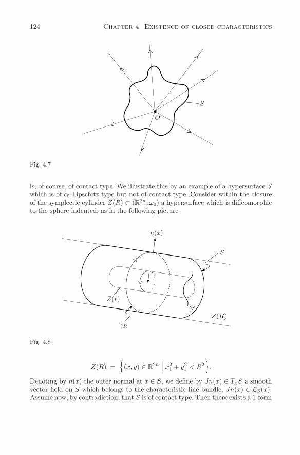
124 Chapter 4 Existence of closed characteristics
O
S
Fig. 4.7
is, of course, of contact type. We illustrate this by an example of a hypersurface Swhich is of c0-Lipschitz type but not of contact type. Consider within the closureof the symplectic cylinder Z(R) ⊂ (R2n, ω0) a hypersurface which is diffeomorphicto the sphere indented, as in the following picture
Z(r)
n(x)
γR
S
Z(R)
Fig. 4.8
Z(R) =(x, y) ∈ R
2n∣∣∣ x2
1 + y21 < R2
.
Denoting by n(x) the outer normal at x ∈ S, we define by Jn(x) ∈ TxS a smoothvector field on S which belongs to the characteristic line bundle, Jn(x) ∈ LS(x).Assume now, by contradiction, that S is of contact type. Then there exists a 1-form
4.3 Hypersurfaces of contact type, the Weinstein conjecture 125
α near S satisfying dα = ω0 and either
α(Jn(x)
)> 0 , for all x ∈ S
or α(Jn(x)) < 0 for all x ∈ S. Without loss of generality we assume the firstalternative to hold. Define the 1-form λ on R
2n by
λ =n∑
j=1
yj dxj ,
where (x, y) ∈ R2n. Then dλ = ω0 and, therefore, dλ = dα on S. Hence, in view
of H1(S) = 0 we find a smooth function ρ : S → R satisfying α − λ = dρ.Consequently, for every periodic solution γ of the vector field Jn on S,
∫
γ
α =∫
γ
λ > 0.
However, for the two distinguished periodic solutions γR and γr on the outerrespectively inner cylinder, as depicted in the above figure, one finds
∫
γR
λ = πR2 and∫
γr
λ = −πr2.
This contradiction shows that S is not of contact type. Evidently, there is a pa-rameterized family (Sε) modelled on S for which c0(Bε, ω0) = π(R + ε)2 agreeswith the capacity of the cylinders, where Sε = ∂Bε. Therefore, S = S0 is of c0-Lipschitz type. We remark that the argument above also shows that the actions ofall periodic solutions on a compact energy surface S of contact type and satisfyingH1(S) = 0 have all the same sign. In particular, the actions never vanish on suchhypersurfaces.
We conclude this section with a recent result in dimension 3, which is notobtained by the variational methods described so far. We consider a smooth closedand orientable manifold W of dimension 2n− 1. A contact form on W is a 1-formλ such that λ∧ (dλ)n−1 is a volume form on W . Such a contact form determines aso-called contact structure which is the (2n−2) dimensional plane field ξλ definedby
ξλ = Kern(λ) ⊂ TW .
Moreover, the kernel of dλ is 1-dimensional. Thus there exists a unique vector fieldX = Xλ satisfying
iX dλ ≡ 0 and iXλ = 1 .
This distinguished non vanishing vector field on W is called the Reeb vector fieldassociated to λ. Note that we no longer require that W = ∂M and dλ = ω|M fora compact symplectic manifold (M,ω) of dimension 2n.
126 Chapter 4 Existence of closed characteristics
We shall say that the Weinstein conjecture holds true for the manifold W , iffor every contact form λ on W , the associated Reeb vector field Xλ has a closedorbit.
Theorem 7. (H. Hofer) The Weinstein conjecture holds true for the three dimen-sional sphere S3.
Actually the Weinstein conjecture holds true also for every closed orientablethree manifold W 3 satisfying π2(W 3) = 0, see H. Hofer [118] (1993). The proofis based on first order elliptic partial differential equations of “Cauchy-Riemann”type and is influenced by Gromov’s theory of pseudoholomorphic curves in sym-plectic manifolds [107] and Eliashberg’s outline of filling techniques using holo-morphic discs [73].
We point out that there are many contact forms λ on S3, (namely the so-calledovertwisted contact forms) which do not admit an embedding of S3 into R
4 suchthat the induced Hamiltonian flow is conjugated to the Reeb flow defined by Xλ.
Here a contact form λ on a closed three dimensional manifold W is calledovertwisted by Eliashberg, if there exists an embedded disc F D2, where D2 =z ∈ C| |z| ≤ 1, such that
T (∂F ) ⊂ ξλ | ∂F
TxF ⊂ ξλ,x for all x ∈ ∂F .
In the classical work of Lutz [144] and Martinet, [147] contact structures are es-tablished in every compact orientable three-manifold. On S3, in particular, thereexist overtwisted contact structures which are not equivalent by a diffeomorphism(in the sense described below).
A contact form λ which is not overtwisted is called tight. By a deep classificationresult of Eliashberg [74] there is, up to diffeomorphisms however only one contactstructure on S3 which is tight. More precisely, if λ1, λ2 are tight forms on S3, thenaccording to Eliashberg there exists a smooth function f : S3 → R\0 and adiffeomorphism ψ : S3 → S3 satisfying
ψ∗ λ2 = f λ1 .
We shall show now that, for a tight contact structure on S3, the associated Reebvector field has a periodic solution. Represent S3 as the subset of C
2 given by(z1, z2)| |z1|2 + |z2|2 = 1. Writing zj = qj + ipj with qj , pj ∈ R, we define theone-form λ0 on C
2 by
λ0 =12
2∑j=1
(pjdqj − qjdpj)
so that dλ0 = ω0. Due to a fundamental result by Bennequin [20], the specialcontact form λ0|S3 is tight. Consequently, given any tight contact form λ on S3,
4.4 “Classical” Hamiltonian systems 127
we find a nonvanishing function f : S3 → R\0 and a diffeomorphism ψ of S3
such thatψ∗λ = f · (λ0|S3) .
Hence the Reeb flows for λ and f ·(λ0|S3) are conjugated. We can use this in orderto prove that Xλ has, in this special case, a periodic orbit. Since Xfλ0 = −X−fλ0
we may assume that f is positive. We claim that there is a smooth hypersurfaceS ⊂ C
2 bounding a star-shaped domain and a diffeomorphism ψ : S3 → S suchthat
Tψ(Lfλ0) = LS ,
where Lfλ0 is the line bundle of S3 defined by the Reeb vector field associated tofλ0, and where LS is the canonical line field induced on the hypersurface S bythe standard symplectic structure ω0 in C
2 ∼= R4. Indeed, we simply define the
hypersurface S byS =
√f(z) z | z ∈ S3 ⊂ C
2
and the diffeomorphism ψ : S3 → S by ψ(z) =√
f(z)z. Observing now thatλ0(z) = 1
2ω0(z, ·), z ∈ C2 we abbreviate σ =
√f and compute, for z ∈ S3 and
h ∈ TzS3,
ψ∗(λ0|S) (z;h) = 12ω0
(σ(z)z, (dσ(z)h)z + σ(z)h
)
= σ(z)2 12ω0(z, h)
= (f · λ0)(z, h) .
From this, the claim follows. Using the existence result of P. Rabinowitz provedabove, we conclude that the Reeb vector field Xfλ0 has a periodic solution.
To sum up, we have demonstrated that in the exceptional case of a tight contactstructure λ on S3, the associated Reeb vector field Xλ possesses at least one closedorbit.
4.4 “Classical” Hamiltonian systems
The positions of a conservative system of n degrees of freedom are points in theso-called configuration space, which we assume to be an n-dimensional smoothmanifold N . The motion of the system, in the setting of Lagrangian mechanics,is determined by a Lagrangian L defined on the tangent bundle TN of N . This2n-dimensional manifold is called the phase space of the system. In our setting ofHamiltonian mechanics, the motion of the system is determined by a Hamiltonianfunction H defined on the cotangent bundle T ∗N of N . This is the basic example ofa symplectic manifold. It is equipped with a canonical symplectic structure whichwe shall recall first.
If N is any manifold of dimension n, and if TxN is the tangent space at x ∈ N ,we denote its dual space, the so called cotangent space by T ∗
x N . It is the space of
128 Chapter 4 Existence of closed characteristics
linear forms defined on the vector space TxN . The union of all cotangent spacesis called the cotangent bundle of N and denoted by
T ∗N =⋃
x∈N
T ∗x N.
A point α in this set M = T ∗N is a linear form αx in the tangent space TxN atsome point x ∈ N , and we shall sometimes use the notation
ξ = (x, ξx) ∈ T ∗N
for a point in M . One can view T ∗N as a differentiable manifold of dimension 2n byintroducing local coordinates, e.g., as follows. If (x1, . . . , xn) are local coordinatesin N , a 1-form α ∈ T ∗
x N is represented by α =∑n
j=1 yjdxj having the coordinates(y1, . . . , yn) and together (x1, . . . , xn, y1, . . . , yn) form local coordinates in T ∗N .In these coordinates one can now define the special 1-form λ on T ∗N by
λ =n∑
j=1
yj dxj ,(4.7)
which has, so far only a local meaning. It is remarkable that the above form λ hasa global interpretation on T ∗N . Since a point of T ∗N is represented by a 1-formξ at a point x ∈ N we can form ξ(V ) for every vector V ∈ TxN . To define aone-form on T ∗N , say β, one has to give its value β(X) for every tangent vectorX of T ∗N . If X is such a tangent vector at ξ ∈ T ∗N , one can use the form ξ itselfto define
λξ(X) = ξ(dπX) , X ∈ Tξ(T ∗N )(4.8)
as a linear functional. Here the projection π : T ∗N → N assigns to each ξ ∈ T ∗Nits base point x ∈ N and, therefore, dπ maps the tangent space Tξ(T ∗N ) at ξonto the tangent space TxN at x. This 1-form λ on T ∗N is sometimes called thetautological form on T ∗N since it is defined in terms of itself. It is readily verifiedthat in the above local coordinates the form (4.8) agrees with the form (4.7). Inview of the expression (4.7) we find
dλ =n∑
j=1
dyj ∧ dxj
and conclude that, globally, ω = dλ is a closed and nondegenerate 2-form onT ∗N , hence a symplectic form. It is called the canonical symplectic structure onT ∗N . The canonical 1-form λ on T ∗N is called the Liouville form. As an aside, weobserve that λ has the distinguished property that
β∗λ = β
4.4 “Classical” Hamiltonian systems 129
for every one-form β on N . Here the one-form β is regarded as a section β : N →T ∗N . The proof follows from the observation that π β = id on N . Consideringthe definition of λ and using the chain rule, we find
(β∗λ)x = λ(x,βx) (dβ)x = βx dπ(x,βx) (dβ)x = βx
as claimed. Classical mechanical systems are described by Hamiltonian functionson (T ∗N, dλ) given by a sum of kinetic energy and the potential energy. Thekinetic energy is defined by a Riemannian metric k on the configuration space,which associates with every point x ∈ N , a symmetric bilinearform kx(v, w) forv, w ∈ TxN which is positive. This metric defines a bundle isomorphism γ : TN →T ∗N by γ(v)(w) = k(v, w) which induces the associated Riemannian metric K onthe cotangent bundle T ∗N by
K(ξ, η) = k(γ−1(ξ), γ−1(η)
).
The potential energy is represented by a smooth function V : N → R on theconfiguration space. On T ∗N the Hamiltonian H is now defined by
H(ξ) = K(ξ) + V(π(ξ)
), ξ ∈ T ∗N.(4.9)
In the above local coordinates we have the formulae:
H = K(x, y) + V (x)
λ =n∑
j=1
yj dxj
XH =n∑
j=1
(∂K
∂yj
∂
∂xj− ∂H
∂xj
∂
∂yj
)(4.10)
λ(XH
)=
n∑j=1
yj∂K
∂yj= 2K ,
where K(x, y) = 12〈S(x)y, y〉 with a positive definite matrix S(x).
If ξ(t) is a solution of the Hamiltonian vector field XH contained in the invariantenergy surface
S =
ξ∣∣∣ H = K + V = E
,(4.11)
then the geometric motion of the system in the configuration space is given byx(t) = π(ξ(t)) ∈ N where π : T ∗N → N is the projection. Since K ≥ 0, it isconfined in the subset
NE =
x ∈ N∣∣∣ V (x) ≤ E
.(4.12)
130 Chapter 4 Existence of closed characteristics
If E < max V , this set is an n-dimensional manifold having the smooth boundary∂NE = V (x) = E provided S is a regular energy surface. Indeed, where K = 0we also have ∂
∂yK = 0 so that necessarily ∂∂xV (x) = 0 on V (x) = E. However
if E > max V , then NE = N is the whole configuration space and K > 0 on S.Therefore λ(XH) = 2K > 0 on S and we see that S is a hypersurface of contacttype whose contact structure is defined by means of the Liouville form λ. If thecapacity c0(U) is finite for a neighborhood U of S in T ∗N we can conclude that Sadmits a closed characteristic. Unfortunately, nothing is known about the specialcapacity c0 on cotangent bundles, except in the special case of the torus which willbe treated later.
Periodic solutions on S have been found by using geometrical ideas, as we shallbriefly indicate next. Assuming that E > max V , we have
T ∗NE = T ∗N
and we can define the special Riemannian metric G on T ∗N by
G(ξ) =K(ξ)
E − V(π(ξ)
) , ξ ∈ T ∗N.
It is the so-called Jacobi metric. We have now two Hamiltonian functions, namelyH and G, which describe S as the regular energy surface
S =
H(ξ) = E
=
G(ξ) = 1.
The corresponding Hamiltonian vector fields are, therefore, parallel, XH = ρXG onS, with a nonvanishing function ρ defined on S which is actually easily computedin local coordinates. One finds that
XH = K · XG on S.
Consequently, the vector fields XH and XG have, on S, the same orbits up toreparametrization. Geometrically, the vector field XG generates the geodesic flowdefined by the Riemannian metric G on T ∗N . The projection π(ξ(t)) of a flow lineis a geodesic line in the configuration space N , i.e., it locally minimizes the lengthbetween two points, where the length is measured with respect to the metric g onTN given by
gx(v, w) =(E − V (x)
)−1
kx(v, w) , with v, w ∈ TxN.
We see that the geodesics for the Riemannian metric G on T ∗N agree, up toreparametrization, with the solutions of the Hamiltonian vector field XH on S. Thisholds true, of course, only on the distinguished energy surface S. This fact is knownas the Euler-Maupertuis-Jacobi principle. It reduces the dynamical problem of
4.4 “Classical” Hamiltonian systems 131
finding solutions for the Hamiltonian vector field on S to the geometrical problemof finding geodesics for the Jacobi metric on N , a problem with a rich history.
Recall that if N is not simply connected, e.g., a torus, one can consider thefamily of closed curves in a nontrivial homotopy class and obtain a closed geodesicof shortest length. This was already known to Hadamard 1889. Technically thisapproach requires that the length functional on the subspace of loops attains itsminimum, an analytical problem which was clearly seen and attacked by D. Hilbert(1890), see [112]. To find closed geodesics on a Riemannian manifold N which issimply connected is a difficult and interesting task. In this case the geodesics cannotbe found as minima but rather as saddle points of the length functional using thetopology of the loop space of the underlying manifold N . G. Birkhoff establisheda closed geodesic on the two-spheres using a minimax principle which later led tothe Ljusternik-Schnirelman theory for critical points. The Morse theory developedat roughly the same time had its origin in the existence problem of geodesics.Extending Birkhoff’s idea to higher dimensions, Ljusternik and Fet proved in 1951[81] that every compact Riemannian manifold (N, g) possesses a closed geodesic.From this geometrical result one deduces immediately by taking the Jacobi metricthat the energy surface S above possesses a closed characteristic, provided N iscompact and E > max V .
In the case that E < max V the theory of closed geodesics is not applicabledirectly, since now the manifold NE has a boundary ∂NE where the Jacobi met-ric blows up. Despite this analytical difficulty, S.V. Bolotin [29] 1978 used thegeometrical approach successfully in order to prove:
Theorem 6. Let N be any smooth manifold and assume H : T ∗N → R describes aclassical system of the form (4.9). Then every compact and regular energy surfaceSE possess a periodic solution of XH .
This theorem extends an earlier result by H. Seifert [193] in 1948 which requiresthat NE is homeomorphic to an n-cell. In 1917 G. Birkhoff proved the statementfor NE = S2.
Using the geometric approach, Bolotin’s result has been rediscovered by H.Gluck and W. Ziller (1983) [106] and later on by V. Benci (1984) [18]. We shouldmention that in the case ∂NE = ∅ the periodic solution found by the theorem is aso-called brake orbit. This is one for which the motion π(ξ(t)) in the configurationspace NE moves back and forth between different points of the boundary ∂NE
but otherwise runs through the interior. Note that the systems considered arereversible: if ξ(t) is a solution of XH then −ξ(−t) is also a solution so that witha motion x(t) = π(ξ(t)) in the configuration space the motion x(−t) = π(−ξ(−t))traversed backwards also corresponds to a solution of XH . This situation is, ofcourse, familiar from the 2-dimensional case of a function H(x, y) = 1
2y2 + V (x),
as depicted in the following figure.
There are many results for closed geodesics which, applied to the Jacobi metriclead to closed characteristics of energy surfaces. We refer to Klingenberg’s book
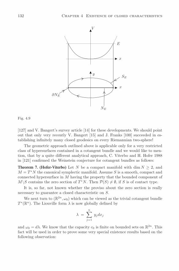
132 Chapter 4 Existence of closed characteristics
V
E
x
ySE
x
∂NE
NE
Fig. 4.9
[127] and V. Bangert’s survey article [14] for these developments. We should pointout that only very recently V. Bangert [15] and J. Franks [100] succeeded in es-tablishing infinitely many closed geodesics on every Riemannian two-sphere!
The geometric approach outlined above is applicable only for a very restrictedclass of hypersurfaces contained in a cotangent bundle and we would like to men-tion, that by a quite different analytical approach, C. Viterbo and H. Hofer 1988in [121] confirmed the Weinstein conjecture for cotangent bundles as follows:
Theorem 7. (Hofer-Viterbo) Let N be a compact manifold with dim N ≥ 2, andM = T ∗N the canonical symplectic manifold. Assume S is a smooth, compact andconnected hypersurface in M having the property that the bounded component ofM\S contains the zero section of T ∗N . Then P(S) = ∅, if S is of contact type.
It is, so far, not known whether the proviso about the zero section is reallynecessary to guarantee a closed characteristic on S.
We next turn to (R2n, ω0) which can be viewed as the trivial cotangent bundleT ∗(Rn). The Liouville form λ is now globally defined by
λ =n∑
j=1
yjdxj
and ω0 = dλ. We know that the capacity c0 is finite on bounded sets on R2n. This
fact will be used in order to prove some very special existence results based on thefollowing observation:
4.4 “Classical” Hamiltonian systems 133
Lemma. Assume the smooth Hamiltonian H : R2n → R satisfies
λ(XH) > 0 for all (x, y) ∈ R2n with y = 0.
Then every compact and regular energy surface S = H(x, y) = E is of contacttype.
Since λ(XH) = 〈 ∂∂y
H(x, y), y〉, and since S is contained in a neighborhoodhaving finite capacity c0, we immediately conclude in view of the lemma andTheorem 5:
Theorem 8. If H ∈ C∞(R2n, R) satisfies
〈 ∂
∂yH (x, y), y〉 > 0 for all (x, y) ∈ R
2n with y = 0,
then every compact and regular energy surface S of H possesses a periodic solutionfor XH .
The assumption is satisfied e.g. for H(x, y) = 12〈A(x)y, y〉 + V (x), with
A(x) > 0, i.e., positive definite.
Proof of the Lemma. If S does not contain points (x, 0) with x ∈ Rn, it is of contact
type as explained above, the contact structure being given by the Liouville form.Otherwise we simply modify the Liouville form and define a 1-form α on R
2n
settingα = λ − εdF ,
where the function F ∈ C∞(R2n, R) is given by
F (x, y) = 〈 ∂
∂xH(x, 0), y〉.
Clearly, dα = dλ = ω0, and we shall show for ε > 0 sufficiently small that α(XH) >0 on S, so that the one-form α meets all the requirements in the definition ofcontact type. By assumption λ(XH) = 〈 ∂
∂yH(x, y), y〉 > 0 if y = 0, so that for
fixed x the function y → 〈 ∂∂yH(x, y), y〉 has a minimum at y = 0 and it follows
that ∂∂yH(x, 0) = 0. A computation shows that
α(XH) = λ(XH) + ε
〈∂H
∂x(x, y),
∂H
∂x(x, 0)〉 −
n∑j,k=1
∂2H
∂xk∂xj(x, 0)
∂H
∂yk(x, y)yj
.
By assumption, dH = 0 on S, hence ∂∂x
H(x, 0) = 0. Consequently, if (x, y) ∈ Sand y is small, the expression in the bracket of the formula above is positive. Onthe other hand, if (x, y) ∈ S and y is bounded away from y = 0, then the firstterm is bounded away from zero and, S being compact, we can choose ε > 0 sosmall that it dominates the second term. Now α(XH) > 0 on S, as we wanted toprove.
By the same argument we have also proved the following, more general, state-ment discovered in 1987 by V. Benci, H. Hofer and P. Rabinowitz [19].
134 Chapter 4 Existence of closed characteristics
Theorem 9. Assume the energy surface S = (x, y) |H(x, y) = E is compact andregular and has the following property: if (x, y) ∈ S and y = 0 then λ(XH) > 0,and if (x, 0) ∈ S then ∂
∂xH(x, 0) = 0. Then S is of contact type and hence XH hasa periodic solution of energy E.
The compactness of the energy surfaces is a crucial assumption for the resultsabove. The existence of periodic solutions on non compact energy surfaces requiresadditional conditions as the example H(x, y) = 1
2 |y|2 in R2n which has no periodic
solutions shows. We would like to mention a result in the non compact case due toD. Offin, in [171] (1985). It states that if the boundary ∂NE in the configurationspace is disconnected while NE itself is connected then (under some additionaltechnical assumptions) there exists a periodic orbit of energy E. This orbit is abrake orbit oscillating between two points belonging to different components of∂NE. Offin obtains the periodic orbit by a direct variational argument minimizingthe energy integral of the corresponding Jacobi metric in the configuration space.
Of special interest in mechanics is the cotangent bundle T ∗(Tn) of the torusTn = R
n/Zn which is isomorphic to Tn × R
n. This symplectic manifold occursas the phase space in many mechanical systems; in particular, for systems whichare close to integrable ones. We shall briefly explain how it arises, referring toAppendix 1 for details. We start from a particularly simple system, a so-calledintegrable system. It is characterized by the property of having sufficiently manyintegrals such that the task of solving (or integrating) the differential equationsbecomes essentially trivial. More precisely, we consider a Hamiltonian system XH0
on a symplectic manifold (M,ω) of dimension 2n. It is called integrable (in thesense of Liouville) if there exist n = 1
2 dim M functions Fj : M → R, 1 ≤ j ≤ n,having the following properties:
(i) dF1, dF2, . . . , dFn are linearly independent on M,
(ii) Fi, Fj = 0 for all i, j,
(iii) H0, Fj = 0 for all j,
where the functions Fi, Fj = ω(XFj, XFj
) are the Poisson brackets. Assume nowthat there exists a level set
Nc∗ =
x ∈ M∣∣∣ Fj(x) = c∗j , 1 ≤ j ≤ n
which is compact and connected. Then one concludes from (i) and (ii) that Nc∗∼=
Tn is an embedded n-dimensional torus, which is Lagrangian. Moreover, thereexists an open neighborhood U of Nc∗ foliated into such tori in which one canintroduce so-called action and angle variables. This means that there exists asymplectic diffeomorphism
ψ : Tn × D −→ U
ψ∗ω = d( n∑
j=1
yj dxj
).
.
4.4 “Classical” Hamiltonian systems 135
Here xj (mod 1) are the angle variables of Tn and y ∈ D are the action variables,where D ⊂ R
n is an open set. Moreover, the functions Fj ψ(x, y) =: fj(y)depend only on the action variables. It then follows from assumption (iii) that theHamiltonian system looks very simple on U , namely
H0 ψ(x, y) = h0(y),
i.e., it depends only on the action variables. What we have described is the Arnold-Jost theorem on the existence of action-angle variables. It extends a local statementwhich goes back to Liouville, and we refer to the Appendix for a proof. TheHamiltonian equation on Tn × D,
x = ∂∂y h0(y)
y = 0,
can be solved explicitly and for all times. Indeed we read off for the flow on Tn×D
ϕt(x, y) = (x + tω, y)
where
ω = ω(y) =∂
∂yh0(y).
Geometrically each torus Tn × y is invariant, the motion on it is linear andgiven by the frequencies ω(y) ∈ R
n. For example, if ω is a rationally independentvector, the orbits are dense on the torus and describe quasi-periodic motions of thesystem. Orbits with ω(y) = j ·α0 for j ∈ Z
n are evidently periodic. These periodicsolutions have Floquet multipliers all equal to 1 and one expects, therefore, thatthe integrability is destroyed immediately under the slightest perturbation of thesystem. Indeed integrable systems are very rare, hence of particular interest; werefer to J. Moser [166] for this topic.
There are, however, many important systems in physics which are close tointegrable systems in the sense that
|H − h0|Ck(T n×D) ≤ ε,
is small, where H(x, y) is a function on Tn × D. In general, the integrabilityis lost under perturbation and the orbit structure of XH is extremely intricate.Nevertheless, the celebrated K.A.M.-theory states that many of the quasi-periodicsolutions of Xh0 can be continued to quasi-periodic solutions of XH provided onlythat ε is sufficiently small, the number k of derivatives is sufficiently large and theintegrable system is nondegenerate in the sense that
det( ∂2
∂y2h0(y)
)= 0.(4.13)
136 Chapter 4 Existence of closed characteristics
This condition requires the system h0 to be nonlinear, so that the frequenciesdepend on the amplitudes. In sharp contrast to these analytically very difficultperturbation results for the existence of special solutions, we shall establish globalperiodic solutions for every system H(x, y) on Tn × R
n assuming, however, thatthe energy surfaces are compact. This will follow from the following result for thecapacities on T ∗(Tn) due to Mei-Yue Jiang [125].
Proposition 4. Let M = Tn × Rn with Tn = R
n/2πZn , equipped with the canonical
symplectic structure ω = d(∑n
j=1 yjdϑj). Then every capacity function c is finiteon open and bounded subsets of M . Moreover, for every a > 0,
c(Tn × (−a, a)n) = 4πa = c(Tn × (−a, a) × Rn−1).
Proof. The proof follows readily from the axioms of a capacity. We start with thesymplectic diffeomorphism ϕ in 2 dimensions:
ϕ : S1 × (−a, a) −→ A =
(x, y) ∈ R2∣∣∣a < x2 + y2 < 5a
given by y =√
3a + 2r cos ϑ, x =√
3a + 2r sinϑ, where 0 ≤ ϑ ≤ 2π and −a < r <+a. Then ϕ∗(dy ∧ dx) = dr ∧ dϑ. Taking a tensor product we find a symplecticdiffeomorphism Tn × (−a, a)n → A×A×· · ·×A ⊂ R
2n, where the product of theannuli corresponds to the symplectic splitting R
2n = R2 ⊕ · · · ⊕ R
2. Therefore itremains to show that c(A × A × · · · × A) = 4πa which is the area of the annulusA. For ε > 0 there exist symplectic embeddings
D(2√
a − ε) −→ A −→ D(2√
a + ε),
where D(R) is the two-disk of radius R. They give rise to symplectic embeddingsfor the product and we conclude that
π(2√
a − ε)2 ≤ c(A × A × · · · × A) ≤ π(2√
a + ε)2.
Since this holds true for every ε > 0 the first equation in the theorem follows; thesecond one is proved the same way.
In particular, the special capacity c0 is finite on bounded open sets of T ∗(Tn)and we can apply all the qualitative existence results obtained so far. We conclude,for example, that a compact hypersurface S ⊂ T ∗(Tn) which is of contact typealways carries a closed characteristic. One can verify, as in the lemma above,that every compact and regular energy surface of a classical system of the formH = 1
2 |y|2 + V (x) on (x, y) ∈ Tn × Rn, where V is periodic in all its variables, is
of contact type and hence possesses a periodic solution of XH . Nothing is known,however, about the nature of this solution. To which homotopy class of loops onT ∗(Tn) does it belong? Is it the brake orbit already guaranteed by Theorem 6?Special periodic solutions for such classical systems can be found by means of theMaupertuis-Jacobi principle, as is shown in the survey article [129] by V.V. Koslov(1985).
4.5 The torus and Herman’s Non-Closing Lemma 137
4.5 The torus and Herman’s Non-Closing Lemma
If ψ : S × (−1,+1) → U ⊂ M is a parameterized family of hypersurfaces modelledon S in a symplectic manifold (M,ω) then U is the union of hypersurfaces Sε =ψ(S × ε), and we know that
c0(U, ω) < ∞ =⇒ there is an ε with P(Sε) = ∅.
Conversely, of course, if P(Sε) = ∅ for every ε then c0(U, ω) = ∞ and, by themonotonicity property of the capacity c0(M,ω) = +∞. We shall next describe anexample due to E. Zehnder[231] which illustrates this situation. We consider themanifold
M = T 3 × [0, 1] , where T 3 = R3/Z
3
is the 3-dimensional torus and define a distinguished symplectic structure on M byslightly modifying the standard structure ω0 on R
4. Recall that to every constantmatrix A satisfying det A = 0 and AT = −A, we can associate the symplecticstructure ω by
ω(X,Y ) = 〈AX, Y 〉on R
4, and then, of course, also on M . A Hamiltonian function H : M → R issimply a function H : R
3 × [0, 1] → R such that H(x1, x2, x3, x4) is periodic inx1, x2, x3 of period 1. The Hamiltonian vector field XH is, as usual, defined by
ω(XH , Y ) = −dH(Y )
for all Y ∈ R4, and one obtains
XH = −A−1 ∇H.
We now define A by setting −A−1 = J∗, and
J∗ =
0 1 0 α1
−1 0 0 α2
0 0 0 1
−α1 −α2 −1 0
,(4.14)
with two real numbers α1, α2 ∈ R. Then det J∗ = 1 and the symplectic formω = ω∗ is the following 2-form:
ω∗ = dx2 ∧ dx1 + dx4 ∧ dx3 + α1 dx3 ∧ dx2 + α2 dx1 ∧ dx3.(4.15)
Choosing the Hamiltonian function H0 : M → R defined as
H0(x) = x4,(4.16)
138 Chapter 4 Existence of closed characteristics
the Hamiltonian vector field on M , given by
XH0 = J∗ ∇H0 = J∗ e4 = (α1, α2, 1, 0),
is constant. The energy surfaces
H−10 (c) =
x ∈ M
∣∣∣ H0(x) = x4 = c
(4.17)
are regular and, since xj ∈ S1 for 1 ≤ j ≤ 3, equal to the 3-dimensional toriH−1
0 (c) = T 3 × c. We introduce the abbreviation
α = (α1, α2, 1) ∈ R3.(4.18)
The flow of the Hamiltonian equations restricted to the energy surfaces T 3 × cis linear and determined by
xk = αk , 1 ≤ k ≤ 3.(4.19)
If we choose α rationally independent, requiring
〈α, j〉 = 0 for 0 = j ∈ Z3,
then all the orbits of (4.19) are dense on T 3, in view of Kronecker’s theorem.Consequently, we have an example of a Hamiltonian system whose energy surfacesare all regular and compact, which, however, does not admit any periodic solution.Incidentally, the energy surfaces are not of contact type.
As an aside, we remark that one can easily construct an embedding ϕ : T 3 ×[0, 1] → R
4. The induced parameterized family of hypersurfaces modelled on T 3
carries no closed characteristic with respect to the pushed forward symplecticstructure which we denote again by ω∗. However, ω∗ on ϕ(M) ⊂ R
4 is not equiv-alent to the standard structure (ϕ(M), ω0) induced from R
4. Indeed, ω0 is anexact symplectic structure, while ω∗ is not; moreover, c0(ϕ(M), ω∗) = +∞ whilec0(ϕ(M), ω0) < ∞. In particular, this example fails to represent a counterexampleto the conjecture that every hypersurface S ⊂ (R2n, ω0) has a closed characteristic.We note that our vector field X on T 3 defined by (4.19) satisfies β(X) = 0 for theclosed 1-form β = dx1 on T 3. Assume now, more generally, that S is any compactmanifold without boundary of dimS = 2n − 1 and that X is a vector field on Ssatisfying β(X) = 0 for a closed 1-form β on S. Then S cannot be embedded as ahypersurface S ⊂ (M,ω) in any symplectic manifold having an exact symplecticstructure, i.e., ω = dλ, such that X ∈ LS, i.e., belongs to the characteristic linebundle. Indeed, suppose it could be, then we could conclude β ∧ (dλ)n−1 to be avolume form on S, since β(X) = 0 and X ∈ ker dλ|S, so that
vol (S) =∫
S
β ∧ (dλ)n−1 = 0 .
4.5 The torus and Herman’s Non-Closing Lemma 139
This, however, is not possible, since the form β ∧ (dλ)n−1 is equal to d(λ ∧ β ∧(dλ)n−2) and hence is an exact form on S.
We now restrict the symplectic structure ω∗ even further by requiring thatα be not only rationally independent but satisfies, in addition, the diophantineconditions
(D.C.) |〈α, j〉| ≥ γ |j|−τ
for all 0 = j ∈ Z3 with two constants γ > 0 and τ > 2. Almost every vector
α ∈ R3 satisfies such conditions. It then turns out that the above example is
actually dynamically stable under perturbations of H0 small with sufficiently manyderivatives. This surprising phenomenon was recently discovered by M. Herman[110, 111], see also J.C. Yoccoz [229]. In our setting he proved
Theorem 10. (M. Herman’s non-closing lemma) Consider the symplectic manifold(M,ω∗) = (T 3 × [0, 1], ω∗) with the symplectic structure (4.15) and α ∈ R
3 satis-fying the conditions (D.C.) Let H0(x) = x4. Then there exists a neighborhood Wof H0
W =
H ∈ Ck(M)∣∣∣ |H − H0|Ck ≤ δ
,
for some small δ > 0 and k > τ + 2, such that for every H ∈ W and every c in12 ≤ c ≤ 3
2 , the regular energy surface
H−1(c) ⊂ M
has no periodic solution for XH .
We note that this dynamical rigidity phenomenon is a property of the specialsymplectic structure ω∗. Postponing the proof we first point out an importantconsequence of Herman’s theorem.
In view of Poincare’s recurrence theorem (see Chapter 1) almost every point xon a compact energy surface for a Hamiltonian system H, is a recurrent point andone may ask whether there exists a nearby system having a periodic trajectorypassing near x. This is the so-called Closing Problem. The answer depends on thenotion of what is “nearby”. In their work [179] (1983) C.C. Pugh and C. Robinsonshowed for the Hamiltonian case, that there is a sequence of Hamiltonian systems,Hj and a sequence of corresponding periodic points, xj for these approximatesystems satisfying
Hj → H in C2 and xj → x.
This is a special case of the celebrated C1-Closing Lemma in [184]. It is a longstanding open question whether Hj can be chosen so that Hj → H in Ck fork > 2. The surprising answer of M. Herman to this question is that on the specialmanifold (M,ω∗) the Ck-Closing Lemma is false, if k is sufficiently large, namely,roughly larger than the dimension of the manifold in question.
140 Chapter 4 Existence of closed characteristics
Proof of Theorem 10. Consider the neighborhood of H0 given by
H = x4 + h(x) and |h|Ck small
on M . The Hamiltonian vector field XH is represented as
XH(x) = J∗ ∇H(x) =
Hx2 + α1Hx4
−Hx1 + α2Hx4
Hx4
−Hx3 − α1Hx1 −α2Hx2
.(4.20)
The energy surface for c, defined by
x4 + h(x) = H(x) = c,
is an embedded torus T 3. Indeed we can solve for x4, and find x4 = K(x1, x2, x3, c),where the function K satisfies the identity
H(x1, x2, x3,K(x1, x2, x3, c)
)= c(4.21)
for all x ∈ T 3. The functions are periodic in x ∈ T 3. To compute the vector fieldXH on H−1(c) we differentiate the identity (4.21) and find Hxj
= −Hx4 · Kxj
on H−1(c) for 1 ≤ j ≤ 3. Therefore, in view of (4.20) the vector field XH is, onH−1(c) given, by
x1
x2
x3
= ρ ·
α1 − Kx2
α2 + Kx1
1
on T 3,(4.22)
where ρ(x) = Hx4(x, K) is a positive function. The vector field (4.22) has, up toreparameterization, the same orbits as
x1
x2
x3
= V (x) :=
α1 − Kx2
α2 + Kx1
1
on T 3.(4.23)
Note that this vector field V on T 3 is a perturbation of the constant vector fieldx = α on T 3, and we can apply a special case of the K.A.M.-theory. We make useof the following result due to J. Moser 1966 in [161].
4.5 The torus and Herman’s Non-Closing Lemma 141
Theorem 11. On the torus Tn = Rn/Z
n consider a vector field of the form
x = α + f(x),
and assume the constant vector α ∈ Rn to satisfy the diophantine conditions
|〈α, j〉| ≥ γ|j|−τ ,
for all 0 = j ∈ Zn with two constants γ > 0 and τ > n − 1. Then, if |f |Cm is
sufficiently small and m > τ + 1, there exist a constant vector λ ∈ Rn and a
C1-diffeomorphism u = id + v : Tn → Tn near the identity, such that
(du)−1 (α + f + λ) u = α .
In other words, if a vector field is near the constant vector field α together withsufficiently many derivatives, it can be modified by constants λ ∈ R
n, so that thismodified vector field is equivalent to α. The proof of this seminal small denominatorresult is based on an analytically subtle iteration technique in infinitely manyspaces and will not be carried out here; we refer to [161].
In general λ = 0, as already the example f = const shows. But in our case thevector field f has an additional structure inherited from the Hamiltonian nature ofthe problem and this additional structure allows us to conclude that λ = 0. Thiswill follow from the
Lemma. Let V be a vector field on the torus Tn satisfying div V = 0. Assume
(du)−1 · V u = α ,
with an irrational vector α ∈ Rn, and a diffeomorphism u = id + v of the torus.
Then u preserves the Lebesgue measure on Tn and∫
T n
V = α.
Postponing the proof of the lemma we first prove Herman’s result. Abbreviatingthe vector field on the right hand side of (4.23) by α+f(x), we first conclude fromTheorem 11 that there exists a λ ∈ R
3 such that the vector field
V : = α + f(x) + λ
is transformed into the constant vector field x = α on T 3. The vector field f has aspecial form inherited from the Hamiltonian structure. Namely
∫f = 0, since the
integrations of derivatives of periodic functions vanish. Consequently,∫
T 3
V = α + λ.
142 Chapter 4 Existence of closed characteristics
In addition, V satisfies div V = 0. Therefore, we conclude by the lemma thatα + λ = α and thus λ = 0. We have proved that the flow of the vector field (4.23)on T 3 is conjugated to the linear flow of x = α and hence has no periodic solutions.This holds true for every constant c in 1
2≤ c ≤ 2
3. The proof of Theorem 10 is
finished, and it remains to prove the lemma.Integrating V u = du(α) and observing that u = id + v we find
∫
T n
V u dµ = α
since the integral over dv(α) vanishes. In order to prove the lemma we only haveto show that u∗µ = µ i.e., preserves the Lebesgue measure. The flow ψt of thevector field V satisfies
(ψt)∗µ = µ.
This is a consequence of the assumption div V = 0. Moreover
u−1 ψt u = Rtα , t ∈ R
with the translations Rtα : x → x + tα on the torus. Therefore ψt u = u Rtα
and in view of (ψt)∗µ = µ we find
u∗µ = (Rtα)∗(u∗µ) , t ∈ R.
By assumption, α is irrational so that all the orbits t → Rtα(x) are dense onTn. Since µ is a constant form we conclude that u∗µ = a · µ with a constant a.Integrating over the torus
∫
T n
µ =∫
T n
u∗µ = a
∫
T n
µ
we find a = 1, proving that indeed u∗µ = µ. This finishes the proof of the lemma. Evidently, also the symplectic manifold (T 4, ω∗) has infinite capacity c0
c0(T 4, ω∗) = +∞
if ω∗ is the particular symplectic structure defined by (4.15) with α = (α1, α2, 1)chosen to be irrational. We know that in the 2-dimensional case c0(T 2, ω) < ∞ forevery volume form ω. It is an open problem whether
c0(T 2n, ω0) < ∞
if n > 1. Here ω0 is the standard symplectic structure induced from R2n.
Chapter 5
Geometry of compactly supportedsymplectic mappings in R
2n
In this chapter we shall study the group D of those symplectic diffeomorphismsof R
2n which are generated by time-dependent Hamiltonian vector fields havingcompactly supported Hamiltonians. We shall construct, in particular, an astonish-ing bi-invariant metric d on D, following H. Hofer [116]. Defining the energy E(ψ)of an element ψ ∈ D by means of the oscillations of generating Hamiltonians, themetric d will be defined by d(ϕ,ψ) = E(ϕ−1ψ). It is of C0-nature. The verificationof the property that d(ϕ,ψ) = 0 if and only if ϕ = ψ, is not easy. It is based onthe action principle. The metric d is intimately related, on the one hand, to thecapacity function c0 introduced in Chapter 3 and hence to periodic orbits and, onthe other hand, to a special capacity e defined on subsets of R
2n and satisfyinge(U) ≥ c0(U). The capacity e is called the displacement energy: e(U) measuresthe distance between the identity map and the set of ψ ∈ D which displaces Ufrom itself, in the sense that ψ(U) ∩ U = ∅. A crucial role in our considerationswill be played by the action spectrum, σ(ψ), of the fixed points of an elementψ ∈ D. It turns out to be a compact nowhere dense subset of R. In contrast to thesimple variational technique used for a fixed Hamiltonian in Chapter 3, a minimaxprinciple will be designed which is applicable simultaneously to all Hamiltoniansgenerating the elements of D. It singles out a distinguished action γ(ϕ) ∈ σ(ϕ).The map γ : (D, d) → R is a continuous section of the action spectrum bundleover D; it is the main technical tool in this section. Its properties will also be usedin order to establish infintely many periodic orbits for certain elements of D, andto describe the geodesics of (D, d). We mention that the completion of the groupD with respect to the metric d is not understood.
5.1 A special metric d for a group D ofHamiltonian diffeomorphisms
We consider the symplectic space (R2n, ω) with the standard symplectic structureω = ω0 and denote by H the vector space of all smooth and compactly supportedHamiltonian functions H = H(t, x) : [0, 1]×R
2n → R. Associated to every H ∈ His a time-dependent Hamiltonian vector field XH on R
2n defined by
iXHtω = −dHt, where Ht(x) = H(t, x).
H. Hofer and E. Zehnder, Symplectic Invariants and Hamiltonian Dynamics, 143Modern Birkhäuser Classics, DOI 10.1007/978-3-0348-0104-1_5, © Springer Basel AG 2011
144 Chapter 5 Compactly supported symplectic mappings
Since the vector field XH has compact support the Hamiltonian equations
x = XH(t, x), x(0) = x0 ∈ R2n
can be solved over the whole time interval [0, 1] for every given initial value x0 ∈R
2n. We thus obtain a 1-parameter family of symplectic mappings ϕtH for t ∈ [0, 1].
It is defined byϕt
H(x0) = x(t),
where x(t) solves the equation for the initial value x0. Clearly ϕtH(x) = x if |x| is
sufficiently large. ByϕH = ϕ1
H
we shall denote the time-1 map of the flow ϕtH and define the group D of compactly
supported Hamiltonian diffeomorphisms by
D = ϕH | H ∈ H.
Recall that the support of a map ϕ is defined as the closed set supp(ϕ) = closx | ϕ(x) = x. Every compactly supported symplectic diffeomorphism can beinterpolated this way by the flow of a time-dependent Hamiltonian vector field;however, it is not known whether the Hamiltonian function can be chosen to be inH if n > 2. It follows from results of M. Gromov [107] that in the special case of R
4
the group D is contractible. In particular, every compactly supported symplecticdiffeomorphism ϕ in R
4 can be written as ϕ = ϕH with H ∈ H and, therefore,belongs to D.
It is the aim of this chapter to study some geometric properties of this groupD of Hamiltonian mappings on R
2n. We begin with two preliminary formal state-ments which will be useful later on.
Definition. Given H, K ∈ H and ϑ ∈ D we define the functions H, H#K and Hϑ
in H as follows:
H(t, x) = −H(t, ϕtH (x))
(H#K)(t, x) = H(t, x) + K(t, (ϕtH)−1(x))
Hϑ(t, x) = H(t, ϑ−1(x)).
Proposition 1. For H, K ∈ H the following formulae hold true
ϕtH
= (ϕtH)−1
ϕtH#K = ϕt
H ϕtK
ϑ ϕtH ϑ−1 = ϕt
Hϑ
(ϕtH)−1 ϕt
K = ϕtG
where G = H#K = (K − H)(t, ϕtH)
5.1 A special metric d for a group D . . . 145
Proof. The third formula is the transformation law of Hamiltonian vector fieldsunder symplectic transformations, as we know from the introduction. The firstformula follows from the second one while the last one is a consequence of the firsttwo. To prove the second formula, we abbreviate the notation and observe that
d
dtϕt = XH ϕt and ϕ0 = id
d
dtψt = XK ψt and ψ0 = id.
We have to show that ϕt ψt is the flow of XH#K . Differentiating, we find
d
dt(ϕt ψt) =
( d
dtϕt
) ψt + (dϕt ψt) · d
dtψt
= XH(ϕt ψt) +[dϕt (ϕt)−1 ϕt ψt
]· XK
[(ϕt)−1 ϕt ψt
].
By the transformation law of Hamiltonian vector fields the second term is equalto
XK(ϕt)−1 (ϕt ψt),
and the claim is proved. By definition, a smooth arc in D is a map t → ψt from I = [0, 1] into D such
that (t, x) → ψt(x) is a smooth mapping from I × R2n into R
2n and such thatthere exists a compact set in R
2n containing all the supports of ψt for t ∈ I. Weshall denote by A the set of smooth arcs [0, 1] → D : t → ϕt satisfying ϕ0 = id.
Proposition 2. The map H → ψtH from H into A is a bijection onto A.
Proof. If H and K satisfy ϕtH = ϕt
K for t ∈ I we find by differentiation thatXH = XK . Therefore, dHt = dKt so that H(t, x) = K(t, x) since the functionshave compact support. This proves the injectivity of the map; in order to provethe surjectivity we consider a smooth arc t → ψt in D satisfying ψ0 = id, anddefine the time-dependent vector field
Xt :=d
dtψt (ψt)−1,
so thatd
dtψt = Xt(ψt) and ψ0 = id.
Because of (ψt)∗ω = ω, we have LXtω = 0. In view of dω = 0 we find d(iXt
ω) = 0.The 1-form iXt
ω being closed is exact on R2n, by the Poincare lemma. There is a
function H : I × R2n → R, determined by
H(t, x) = −∫ 1
0
ω(Xt(sx), x)ds ,
146 Chapter 5 Compactly supported symplectic mappings
which satisfies −dHt = iXtω. Since Xt has compact support, dHt(x) = 0, for
t ∈ I and |x| ≥ R, for some large R and there is a K ∈ H with dHt = dKt. It isgiven by H(t, x)−H(t, x∗) for some x∗ with |x∗| ≥ R. Consequently Xt = XKt
asclaimed.
We next define the length of an arc t → ψt belonging to A. In view of Propo-sition 2 there is a unique H ∈ H generating this arc by
ψt = ϕtH .
Define for H ∈ C∞c (R2n, R) the norm (called the oscillation)
||H|| = supx
H(x) − infx
H(x).(5.1)
Then||H ϕ|| = ||H||
for every diffeomorphism ϕ of R2n. If now H ∈ H, we can associate with the
Hamiltonian vector field XHtthe norm ||XHt
|| := ||Ht|| and find∫ 1
0
||ψt|| dt =∫ 1
0
||XHt(ψt)||dt =
∫ 1
0
||Ht|| dt.
Introducing the norm in H by
||H|| =∫ 1
0
||Ht|| dt =∫ 1
0
[supx
H(t, x) − infx
H(t, x)] dt,(5.2)
which agrees for autonomous H with definition (5.1), we are led to define thelength of the arc ψt = ϕt
H connecting ψ1 with id, as
l(ψ[0,1]) = ||H||.(5.3)
Definition. The energy of a symplectic map ψ in D is the number E(ψ) ≥ 0 definedby
E(ψ) = infl(ψ[0,1]) | the arc ψt in A satisfies ψ1 = ψ.
EvidentlyE(ϕH) ≤ ||H||.(5.4)
The Hamiltonian H = 0 in H generates the identity map ψ = id and consequentlyE(id) = 0. Conversely,
E(ψ) > 0, if ψ = id.(5.5)
But this crucial fact is not at all obvious. It follows from the following estimatesfor the energy function in which c0(U) = c0(U, ω) denotes the special capacityintroduced in Chapter 3. For notational convenience we set c0(∅) = 0, and recallthat Z(R) denotes the symplectic cylinder of radius R.
5.1 A special metric d for a group D . . . 147
Theorem 1. (energy-capacity inequality) For every ψ ∈ D
supc0(U) | U open and ψ(U) ∩ U = ∅ ≤ E(ψ)
E(ψ) ≤ 16 infπR2 | there is a ϕ ∈ D with supp (ϕψϕ−1) ⊂ Z(R).
We see, in particular, that the energy E(ψ) is always larger than the capacityc0(U) of every open set U which can be displaced from itself by the map ψ. It isnow easy to deduce the claim (5.5): indeed taking a point x∗ satisfying ψ(x∗) = x∗
there exists an open ball B(x∗, ε) = U of radius ε > 0, which is displaced fromitself, ψ(U) ∩ U = ∅. Using c0(U) = πε2 we thus conclude from Theorem 1 thatE(ψ) ≥ πε2 > 0 proving the claim (5.5).
The proof of the first estimate in Theorem 1 will be based on the existence ofa distinguished critical point of the action functional, it will be carried out in theSections 5.5 and 5.6 below.
Theorem 2. (C0-energy estimate) For every ψ ∈ D
E(ψ) ≤ C diameter supp (ψ) |id − ψ|C
with a constant C ≤ 128.This statement expresses the continuity of E at the identity map in the C0-
topology. The proof of Theorem 2 will also be postponed to Section 5.6 below.
Proposition 3. The energy function E : D → R meets the following properties:
(i) E(ϕ) ≥ 0, and E(ϕ) = 0 ⇐⇒ ϕ = id
(ii) E(ϕ) = E(ϕ−1)
(iii) E(ϑϕϑ−1) = E(ϕ)
(iv) E(ϕψ) ≤ E(ϕ) + E(ψ) ,
where ϕ,ψ ∈ D and where ϑ is a symplectic diffeomorphism of R2n.
Proof. The proofs of (i) and (ii) follow readily from the definition of E using thenontrivial fact (5.5) proved later on. Clearly
l(ϕ[0,1]H ) = l(ϕ[0,1]
H)
implying E(ϕ) = E(ϕ−1). From
ϑ ϕtH ϑ−1 = ϕt
Hϑ
we findl((ϑ ϕH ϑ−1)[0,1]) = l(ϕ[0,1]
Hϑ)
148 Chapter 5 Compactly supported symplectic mappings
implying (iii). Finally, in view of Proposition 1, we have ϕtH ϕt
K = ϕtH#K and
l(ϕ[0,1]H#K) =
∫ 1
0
supx
(H#K)t − infx
(H#K)t dt
≤∫ 1
0
(supx
Ht − infx
Ht) dt +∫ 1
0
(supx
Kt − infx
Kt) dt
= l(ϕ[0,1]H ) + l(ϕ[0,1]
K )
which implies E(ϕH ϕK) ≤ E(ϕH ) + E(ϕK) and the last claim (iv) follows. We can derive an estimate for the commutators in D, denoted by
[ϕ,ψ] := ϕψ ϕ−1 ψ−1 ,(5.6)
and first claim thatE([ϕ,ψ]) ≤ 2 minE(ϕ), E(ψ)(5.7)
for ϕ,ψ ∈ D. Indeed, in view of the statements (ii)–(iv) in Proposition 3 we canestimate E(ϕψϕ−1ψ−1) ≤ E(ϕψϕ−1) + E(ψ−1) ≤ 2E(ψ) and E(ϕψϕ−1ψ−1) ≤E(ϕ)+E(ψϕ−1ψ−1) = 2E(ϕ), hence proving the claim. We now deduce an “a pri-ori” estimate for the energy of commutators of those maps having their supportsin a fixed open set.
Proposition 4. If U ⊂ R2n is open and bounded and if ϑ ∈ D satisfies ϑ(U)∩U = ∅,
thenE([ϕ,ψ]) ≤ 4E(ϑ)
for all ϕ,ψ ∈ D with supp(ϕ) and supp(ψ) contained in U .
Proof. Defineγ := ϕ ϑ−1 ϕ−1 ϑ ∈ D
then γ|U = ϕ|U since ϑ(U)∩U = ∅ and supp(ϕ) ⊂ U . Consequently ϕψϕ−1ψ−1 =γψγ−1ψ−1 on U , and since both maps are the identity maps outside of U , theyare equal on R
2n. Therefore, in view of (5.7) and Proposition 3
E([ϕ,ψ]) = E([γ, ψ]) ≤ 2E(γ) ≤ 2E(ϑ−1) + 2E(ϑ) = 4E(ϑ)
as we wanted to show. Proposition 3 allows us to define a distinguished metric d : D×D → [0,∞], by
means of the energy:d(ϕ,ψ) := E(ϕ−1ψ).(5.8)
In particular, the energy of ψ ∈ D, E(ψ) = d(id, ψ), is the distance from theidentity map and we remark that, in view of the last formula in Proposition 1,
d(ϕ,ψ) = inf‖H − K‖
∣∣∣ H generates ψ and K generates ϕ
.(5.9)
5.1 A special metric d for a group D . . . 149
Theorem 3. The function d is a bi-invariant metric on D, i.e., it satisfies for allϕ,ψ and ϑ belonging to D:
(i) d(ϕ,ψ) ≥ 0 and d(ϕ,ψ) = 0 ⇔ ϕ = ψ
(ii) d(ϕ,ψ) ≤ d(ϕ, ϑ) + d(ϑ, ψ) and d(ϕ,ψ) = d(ψ,ϕ)
(iii) d(ϑϕ, ϑψ) = d(ϕ,ψ) = d(ϕϑ, ψϑ).
Theorem 3 is an immediate consequence of Proposition 3. In the following wecan consider (D, d) as a topological group. Note that our intrinsic metric on D iscontinuous in the C0-metric provided the supports are uniformly bounded. Indeed,in view of Theorem 1 and Theorem 2,
supc0(U)| U open and ψ(U) ∩ ϕ(U) = ∅ ≤ d(ϕ,ψ)
d(ϕ,ψ) ≤ 128 · diameter ( supp ϕ−1ψ) · supx
|ϕ(x) − ψ(x)|(5.10)
for every pair ϕ and ψ belonging to D. The group D admits, in addition, an orderstructure. Define the positive subset D+ ⊂ D by
D+ = ψH | H ∈ H and H ≥ 0
and the negative subset D− ⊂ D by
D− = ψH | H ∈ H and H ≤ 0.
If ϕ ∈ D+ then ϕ−1 ∈ D− and ϑϕϑ−1 ∈ D+ for every symplectic diffeomorphismϑ of R
2n. This follows from Proposition 1. We shall prove later on in Section 5.4that
D+ ∩ D− = id.(5.11)
A partial order structure ≥ on D can, therefore, as we shall prove, be defined asfollows:
ϕ ≥ ψ ⇔ ϕ ψ−1 ∈ D+.(5.12)
Proposition 5. Assume ϕ,ψ and ϑ ∈ D.
(i) If ϕ ≥ ψ and ψ ≥ ϕ then ϕ = ψ
(ii) If ϕ ≥ ψ and ψ ≥ ϑ then ϕ ≥ ϑ.
In addition, if ϕ ≥ ψ, then ϕϑ ≥ ψϑ.
150 Chapter 5 Compactly supported symplectic mappings
Proof. If ϕ ψ−1 ∈ D+ and ψ ϕ−1 ∈ D+, then ϕ ψ−1 ∈ D+ ∩D− and hence by(5.11), we conclude that ϕ = ψ proving (i). Next observe that if ϕ and ψ are inD+ then also ϕ ψ ∈ D+ in view of Proposition 1 implying (ii).
We conclude this section with two observations due to Y. Eliashberg and L.Polterovich [76]. They consider an arbitrary bi-invariant pseudo-metric ρ : D×D →[0,∞). By definition this ρ satisfies the properties (i)–(iii) of Theorem 3, exceptthat it is not required that ρ(ϕ,ψ) = 0 if ϕ = ψ. Recalling that E(ψ) = d(id, ψ)and arguing as in the proof of Proposition 4, one finds that
ρ(id, [ϕ,ψ]) ≤ 4ρ(id, ϑ)(5.13)
for all ϕ,ψ and ϑ ∈ D satisfying ϑ(U) ∩ U = ∅ and supp(ϕ), supp(ψ) ⊂ U , forsome open set U ⊂ R
2n. Following H. Hofer [116] one can associate with ρ theso-called displacement energy eρ(U) of an open and bounded subset U ⊂ R
2n bydefining
eρ(U) := inf ρ(id, ϑ) | ϑ ∈ D satisfies ϑ(U) ∩ U = ∅.(5.14)
It then follows from (5.13) that
4eρ(U) ≥ ρ(id, [ϕ,ψ])
for every pair ϕ and ψ ∈ D having their supports contained in U . If ρ is notonly a pseudometric but a metric, then ρ(id, [ϕ,ψ]) > 0 provided ϕ and ψ do notcommute. Consequently eρ(U) > 0 and we have proved
Proposition 6. If ρ is a bi-invariant metric on D then the displacement energy eρ
is positive on open sets.This applies in particular to our distinguished bi-invariant metric ρ = d. Note,
however, that the metric character of this d is concluded from the nontrivial esti-mate in Theorem 1 from which it follows that ed(U) ≥ c0(U) > 0 for every openset U . The special displacement energy ed will be studied in more detail later on.
In order to construct the intrinsic bi-invariant metric d on D we started offfrom the sup-norm ||H|| on C∞
c (R2n). We can, of course, start off as well from theLp-norm
||H||p := (∫
|H(x)|p dx)1p
which is evidently invariant under D, i.e., ||H ϕ||p = ||H||p if ϕ ∈ D. We thusarrive at dp(ϕ,ψ) = Ep(ϕψ−1) which defines a bi-invariant pseudometric on D. Itturns out, however, that this dp for 1 ≤ p < ∞ is not a metric. This has recentlybeen proved by Y. Eliashberg and L. Polterovich [76]. They showed, more precisely,that
Ep(ψ) = 0, if p = 1,
for every ψ ∈ D having vanishing Calabi invariant, i.e.,∫ 1
0
∫R2n
H(t, x) dx dt = 0
if ψ = ψH for H ∈ H. Moreover, Ep(ψ) = 0 for all ψ ∈ D provided 1 < p < ∞.
5.2 The action spectrum of a Hamiltonian map 151
5.2 The action spectrum of a Hamiltonian map
For H ∈ H we shall denote the set of fixed points of the associated Hamiltonianmap ϕH by
Fix(ϕH ) = x ∈ R2n | ϕH(x) = x.
If x0 ∈ Fix(ϕH ) then the solution x(t) = ϕtH(x0) for 0 ≤ t ≤ 1 of the Hamiltonian
equation x = XH(x) satisfies x(1) = x(0) and hence is a loop in R2n. Its action is
the real number A(x0,H) defined by
A(x0,H) =∫ 1
0
12〈−Jx(t), x(t)〉 −
∫ 1
0
H(t, x(t)) dt.
It turns out that A(x0,H) depends only on the fixed point x0 and the map ϕH
and is independent of the choice of the function H generating the map.
Lemma 1. If H and K in H generate the same map, i.e., ϕH = ϕK then
A(x0,H) = A(x0,K)
for every x0 ∈ Fix(ϕH) = Fix(ϕK).
Proof. Define the piecewise smooth arc t → ψt by
ψt = ϕtH , for t ∈ [0, 1]
ψt = ϕ2−tK , for t ∈ [1, 2].
Thus for every x ∈ R2n the map t → ψt(x) from [0, 2] into R
2n is a loop and weset
∆(x) =∫ 2
0
12〈−Jx(t), x(t)〉 dt −
∫ 1
0
H(t, x(t)) dt +∫ 2
1
K(2 − t, x(t)) dt
where x(t) = ψt(x). This map x → ∆(x) is evidently smooth and by differentiationin x we obtain
∆′(x)h =∫ 2
0〈 −Jx(t), dψt(x)h〉 dt
−∫ 1
0〈 ∇H(t, x(t)), dψt(x)h〉 dt
+∫ 2
1〈 ∇K(2 − t, x(t)), dψt(x)h〉 dt,
which is equal to 0, since t → ψt(x) is a solution of the Hamiltonian systemassociated to H between [0, 1] and to −K(2 − t, ·) between [1, 2]. For |x| large wehave ∆(x) = 0, since H and K are compactly supported so that x(t) ≡ x fort ∈ [0, 2]. This shows that ∆ ≡ 0.Hence if x0 ∈ Fix(ϕH) then A(x0,H) − A(x0,K) = ∆(x0) = 0 as claimed.
In view of the lemma we can associate with a fixed point x0 of the map ψ ∈ Dthe action A(x0, ψ) defined by
A(x0, ψ) = A(x0,H), if ψ = ϕH .
152 Chapter 5 Compactly supported symplectic mappings
Definition. The action spectrum of ϕ ∈ D is the set σ(ϕ) ⊂ R defined by
σ(ϕ) = A(x, ϕ) | x ∈ Fix(ϕ).
Clearly 0 ∈ σ(ϕ) since the Hamiltonians have compact supports. We shall showthat the action spectrum is invariant under symplectic conjugation. More generally,denote by G the group of conformally symplectic diffeomorphisms. By definition,ϑ ∈ G satisfies
ϑ∗ω = αω(5.15)
for some constant α = α(ϑ) ∈ (0,∞). Note that if ϕ = ϕH , then
ϑ ϕtH ϑ−1 = ϕt
αHϑ, where Hϑ(t, x) = H
(t, ϑ−1(x)
).(5.16)
Proposition 7. If ϕ ∈ D and ϑ ∈ G with ϑ∗ω = αω then
In particular,
A(ϑ(x), ϑϕϑ−1) = αA(x, ϕ).
σ(ϑϕϑ−1) = ασ(ϕ).
Proof. Assume ϕ = ϕH and choose x ∈ Fix(ϕ). In view of Lemma 1 and (5.16)we have to show that A(ϑ(x), αHϑ) = αA(x, H). We set
x(t) = ϕtH(x)
y(t) = ϑ(x(t)
)= ϑ ϕt
H ϑ−1(ϑ(x)
)= ϕt
αHϑ
(ϑ(x)
).
Let λ be a primitve of ω, i.e., dλ = ω, then ϑ∗λ−αλ = dF for a function F . Sincethe integral of a closed form over a loop vanishes, we find
A(ϑ(x), αHϑ
)=
1∫0
12〈−Jy(t), y(t)〉 dt −
1∫0
αHϑ
(t, y(t)
)dt
=∫y
ϑ∗λ −1∫0
αHϑ
(t, y(t)
)dt
= α∫x
ϑ∗λ − α1∫0
H(t, x(t)
)dt = αA(x,H) .
The following property of the action spectrum will be crucial later on.
Proposition 8. The action spectrum σ(ϕ) is compact and nowhere dense.
5.2 The action spectrum of a Hamiltonian map 153
Proof. We first show that σ(ϕ) is compact. Assume ϕ = ϕH and recall that forx0 ∈ Fix(ϕ) the loop x(t) = ϕt
H(x0) is a solution of
x(t) = XH(x(t)), and x(1) = x(0) = x0.
Since H has compact support we find an R > 0 such that x(t) = x0 is constant for|x0| ≥ R and hence A(x0, ϕ) = 0. It is, therefore, sufficient to consider fixed pointsx0 for which |x(t)| ≤ R. It then follows that A(x0, ϕ) ≤ M for all x0 ∈ Fix(ϕ) sothat σ(ϕ) is bounded. To prove the compactness we consider a sequence xj(t) ofsolutions corresponding to the fixed points xj = xj(0) and satisfying |xj(t)| ≤ R.By means of the Arzela-Ascoli theorem we find a subsequence satisfying xj(t) →x∗(t) in C∞([0, 1], R2n) and x∗(0) = x∗ ∈ Fix(ϕ). Consequently A(xj , ϕ) →A(x∗, ϕ) implying the compactness of σ(ϕ).
It remains to prove that σ(ϕ) is nowhere dense. We first remark that the loop
x(t) = ϕtH(x0) ∈ C∞([0, 1], R2n)
satisfying x(1) = x(0) = x0 is an element of the Sobolev space E = H1/2(S1, R2n)introduced in Chapter 3. Indeed, its Fourier coefficients xk ∈ R
2n are, after twopartial integrations, estimated by
|xk| ≤ (1
2π|k| )2(|x(1) − x(0)| + |x|C0) ,
for k ∈ Z. Moreover, as in Chapter 3, one verifies that these special loops areprecisely the critical points of the variational functional
aH(x) = a(x) − bH(x), x ∈ E,
where now H ∈ H and
bH(x) =∫ 1
0
H(t, x(t)) dt.
Consequently A(x0, ϕ) = aH(x), with x(t) = ϕtH(x0), is a critical level of aH . In
order to show that the set σ(ϕ) of critical levels is nowhere dense, we follow an ideadue to J.C. Sikorav [198] and construct a smooth function on R
2n whose criticallevels contain σ(ϕ). We extend the function (t, x0) → ϕt
H(x0) : [0, 1] × Fix(ϕ) →R
2n to a smooth function ψ : [0, 1] × R2n → R
2n satisfying
ψ(t, x0) = ϕt(x0), if x0 ∈ Fix(ϕ)
ψ(1, x) = ψ(0, x) for all x ∈ R2n.
To do so simply take a smooth f : [0, 1] → [0, 1] which is equal to 1 near 0 andequal to 0 near 1 and set
ψ(t, x) = f(t)ϕt(x) + [1 − f(t)]ϕt((ϕ1)−1(x)),
154 Chapter 5 Compactly supported symplectic mappings
where ϕt = ϕtH . For every x ∈ R
2n, the map t → ψ(t, x) represents a loop belongingto E and we can define the smooth function Ψ : R
2n → E by setting Ψ(x)(t) =ψ(t, x). Using now the fact (proved in Appendix 3), that aH ∈ C∞(E, R) we havea smooth function defined by
aH Ψ : R2n → R.
It has the property that every x0 ∈ Fix(ϕ) is a critical point of aH Ψ. In addition,A(x0, ϕ) = aH Ψ(x0) is a critical level. Since by Sard’s theorem the set of criticallevels of aH Ψ is nowhere dense, we conclude that also σ(ϕ) is nowhere dense.This finishes the proof of the proposition.
Over the group D we can define the action spectrum bundle A → D by
A =⋃
ϕ∈Dϕ × σ(ϕ) ,
equipped with the metric induced from (D, d)×R. Every fibre is a compact nowheredense set; a generic fibre consists of isolated points except possibly the point 0.Since 0 ∈ σ(ϕ) for every ϕ ∈ D there is a trivial continuous section of A. Theaction spectrum σ(ϕ) does not depend continuously on ϕ ∈ D. In the next twosections we shall construct a nontrivial continuous section
γ : D −→ A ,
i.e., γ(ϕ) ∈ σ(ϕ) and γ ≡ 0. It is, in addition, monotone and invariant undersymplectic conjugation. The existence of this distinguished continuous section isestablished by means of a minimax argument for the action functional.
5.3 A “universal” variational principle
The results in the first section are based on a variational principle to which wewill now turn. Our aim is to establish the existence of a special critical point ofthe action functional
aH(x) = a(x) − bH(x), x ∈ E
introduced in Chapter 3. In contrast to the principle used there, we shall designa minimax principle which is independent of the choice of H ∈ H. Recall thatE is the Hilbert space E = H1/2(S1, R2n) which splits into an orthogonal sumE = E− ⊕ E0 ⊕ E+, and, if x = x− + x0 + x+, then
a(x) =12||x+||2 − 1
2||x−||2
and
bH(x) =∫ 1
0
H(t, x(t)) dt.
5.3 A “universal” variational principle 155
As in Chapter 3 one verifies that the special solutions x ∈ C∞([0, 1], R2n)
x(t) = ϕtH(x0) and x0 ∈ Fix(ϕH )
of the Hamiltonian equation x = XH(x) agree with the critical points of aH on E.We shall single out a family F of subsets F ⊂ E such that for every H ∈ H
γ(H) := supF∈F
infx∈F
aH(x)
is a real number and a critical value of aH . The crucial point will be that F isindependent of the choice of H ∈ H and therefore a “universal” minimax set for H.Later on this will be important for us for the following reason: whenever one hasa family of functionals together with a “universal” minimax set F , we concludefrom the pointwise estimate Φ ≤ Ψ for two functionals in our family the sameinequality for the associated minimax values. Note that
aH(x+) → +∞ as ||x+|| → ∞
where x+ ∈ E+, while
aH(x− + x0) ≤ M for all x− + x0 ∈ E− ⊕ E0
with a constant M depending on H.In order to define F we first introduce a distinguished group of homeomor-
phisms of E, which is prompted by the structure of the gradient flows of aH .
Definition. We define a set G of homeomorphisms of E as follows. A homeomor-phism h belongs to G if h and h−1 map bounded sets onto bounded sets and thereexist continuous maps γ± : E → R and k : E → E mapping bounded sets intoprecompact sets and such that there exist r = r(h) satisfying
k(x) = 0, γ±(x) = 0
for all x ∈ E+ with ||x|| ≥ r. Moreover,
h(x) = eγ+(x)x+ + x0 + eγ−(x)x− + k(x)
for all x ∈ E.
Lemma 2. G is a group.
Proof. We have to show that with h, g ∈ G also h−1 and h g ∈ G. By assumptionon h we have
e−γ±P±h(x) = x± + e−γ±
P±k(x)
P 0h(x) = x0 + P 0k(x).
156 Chapter 5 Compactly supported symplectic mappings
Hence
x = x− + x0 + x+
= e−γ−(x)P−h(x) + P 0h(x) + e−γ+(x)P+h(x)
−(e−γ−(x)P− + P 0 + e−γ+(x)P+)k(x).
Writing x = h−1(y) and y = h(x) we obtain for y = y− + y0 + y+
h−1(y) = e−γ−(h−1(y))y− + y0 + e−γ+(h−1(y))y+
− (e−γ−(h−1(y))P− + P 0 + e−γ+(h−1(y))P+)k(h−1(y))
=: eσ−(y)y− + y0 + eσ+(y)y+ + k(y).
Using the properties of γ± and k together with the fact that h−1 maps boundedsets into bounded sets we conclude that σ± and k have the desired properties andh−1 ∈ G. Similarly one verifies that h g ∈ G.
The distinguished family F of subsets of E is defined by
F = h(E+) | h ∈ G.
The crucial topological property of G lies in the following intersection result whichis intuitively clear:
Lemma 3. If h ∈ G, then
h(E+) ∩ (E− ⊕ E0) = ∅.
Proof. We have to find x ∈ E+ satisfying P+h(x) = 0. This is equivalent toeγ+(x)x + P+k(x) = 0 and x ∈ E+, or
x = −e−γ+(x)P+k(x) =: T (x) , and x ∈ E+ .
The operator T : E+ → E+ maps E+ into a precompact subset of E+ and henceT : B → B for a sufficiently large ball B, so that Schauder’s fixed point theoremguarantees a solution proving the lemma.
Theorem 4. Assume H ∈ H, then γ(H), defined by
γ(H) := supF∈F
inf aH(F ),
is a critical value of aH .
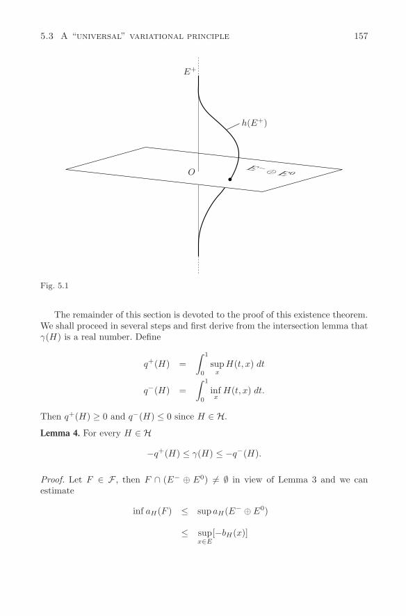
5.3 A “universal” variational principle 157
E+
h(E+)
OE −⊕ E 0
Fig. 5.1
The remainder of this section is devoted to the proof of this existence theorem.We shall proceed in several steps and first derive from the intersection lemma thatγ(H) is a real number. Define
q+(H) =∫ 1
0
supx
H(t, x) dt
q−(H) =∫ 1
0
infx
H(t, x) dt.
Then q+(H) ≥ 0 and q−(H) ≤ 0 since H ∈ H.
Lemma 4. For every H ∈ H
−q+(H) ≤ γ(H) ≤ −q−(H).
Proof. Let F ∈ F , then F ∩ (E− ⊕ E0) = ∅ in view of Lemma 3 and we canestimate
inf aH(F ) ≤ sup aH(E− ⊕ E0)
≤ supx∈E
[−bH(x)]
158 Chapter 5 Compactly supported symplectic mappings
≤ −∫ 1
0
infx
H(t, x) dt.
Since
inf aH(E+) ≥ −∫ 1
0
supx
H(t, x) dt ,
the lemma follows. If γ(H) = 0, then γ(H) is a critical level which contains in particular all the
constant solutions outside of the support of H. We, therefore, only have to showthat γ(H) = 0 is a critical value of aH . For this we need the following compactnessproperty.
Lemma 5. Assume γ(H) = 0 and assume the sequence xj ∈ E satisfies
∇aH (xj) → 0, and aH(xj) → γ(H).
Then xj possesses a convergent subsequence.
Proof. We recall from Chapter 3 that
∇aH(x) = x+ − x− −∇bH(x),
where ∇bH : E → E is globally Lipschitz continuous and maps bounded sets intoprecompact sets. Moreover ∇bH(x) = j∗∇H(x) with the L2-gradient ∇H(x) ofbH .
Assume that the sequence xj ∈ E is bounded in E. Then ∇bH(xj) is pre-compact and taking a subsequence we may assume that ∇bH(xj) → y in E. Byassumption ∇aH(xj) → 0 so that x+
j −x−j → y. In addition, since dimE0 < ∞, we
find a subsequence such that also x0j converges and we see that xj has a convergent
subsequence.Therefore, we only have to prove that the sequence xj is bounded. Arguing in-
directly we may assume by taking a subsequence that ||xj || → +∞. Since H ∈ Hthe sequence ∇H(xj) is bounded in L2 so that ∇bH(xj) = j∗∇H(xj) is precom-pact in E. Hence, taking a subsequence, x+
j − x−j → y in E and also in L2. This
implies that |x0j | → ∞. Consequently we find a subsequence such that pointwise
|xj(t)| → ∞, for a.e. t
implying that H(t, xj(t)) → 0 for a.e. t. Hence by Lebesgue’s theorem, bH(xj) → 0.Also ∇H(t, xj(t)) → 0 for a.e. t so that ∇H(xj) → 0 in L2 and consequently∇bH(xj) → 0 in E. From ∇aH(xj) → 0 we now conclude that x+
j − x−j → 0.
HenceaH(xj) = a(xj) − bH(xj) → 0.
This contradicts the assumption that aH(xj) → γ(H) = 0 and shows that thesequence xj is bounded. The proof of the lemma is finished.
We are ready to finish the proof of Theorem 4 which we reformulate as
5.3 A “universal” variational principle 159
Lemma 6. The real number γ(H) is a critical value of aH , for every H ∈ H.
Proof. Recall that γ(H) is a real number in view of Lemma 4. If γ(H) = 0 there isnothing to prove and we assume γ(H) = 0. In this case the Palais-Smale conditionas formulated in Lemma 5 holds. Arguing by contradiction we assume that γ(H)is not a critical value of aH . Then, in view of Lemma 5, we find an ε > 0 satisfying
|∇aH (x)| ≥ ε, if aH(x) ∈ [γ(H) − ε, γ(H) + ε](5.17)
In order to first slow down the gradient flow we take a smooth map σ : R → [0, 1]satisfying
σ(t) = 1, if t ∈ [γ(H) − ε, γ(H) + ε]
σ(t) = 0, if t ∈ R \ [γ(H) − 2ε, γ(H) + 2ε]
and define σ(x) = σ(aH(x)), for x ∈ E. The flow of the modified gradient equation
x = σ(x)∇aH (x) =: V (x) on E(5.18)
exists for all times and we shall denote it by
(s, x) → x · s : R × E → E.
Using this flow we pick T = 2ε and define the homeomorphism h of E by setting
h(x) = x · T, x ∈ E.(5.19)
By definition of γ(H) there exists an F ∈ F satisfying
F ⊂ x | aH(x) ≥ γ(H) − ε ,
and we shall demonstrate that
h(F ) ⊂ x | aH(x) ≥ γ(H) + ε.(5.20)
Postponing the proof we first show how the lemma is concluded. By definition ofF we have F = g(E+). Therefore, if h ∈ G (a fact which will be proved lateron), then also h g ∈ G since G is a group in view of Lemma 2. Consequentlyh(F ) = h g(E+) ∈ F and we arrive at the contradiction
γ(H) ≥ inf aH(h(F )) ≥ γ(H) + ε,
hence concluding the lemma. In order to verify (5.20) we prove that
aH(x) ≥ γ(H) − ε ⇒ aH(h(x)) ≥ γ(H) + ε.(5.21)
Arguing by contradiction, we assume that aH(h(x)) < γ(H)+ε. Since s → aH(x·s)is monotone-increasing we have
γ(H) + ε > aH(h(x)) ≥ aH(x · s) ≥ aH(x) ≥ γ(H) − ε
160 Chapter 5 Compactly supported symplectic mappings
for all 0 ≤ s ≤ T . Therefore, aH(x · s) ∈ [γ(H) − ε, γ(H) + ε] so that σ(x · s) = 1for 0 ≤ s ≤ T . We see that in this time interval x(s) := x · s solves the gradientequation x = ∇aH(x). Hence using the estimate (5.17) for the gradient:
γ(H) + ε > aH(h(x)) = aH (x · T )
= aH(x) +∫ T
0
|∇aH(x · s)|2ds
≥ γ(H) − ε + Tε2 = γ(H) + ε,
which is a contradiction. The statement (5.21) is verified and it remains to showthat h ∈ G.
Recall thatV (x) = −σ(x)x− + σ(x)x+ − σ(x)∇bH (x).(5.22)
In order to find a representation formula for the flow of x = V (x) on E, we considerfor x ∈ E fixed, the equation
d
dsu = Ax(s)u + fx(s) on E,(5.23)
where Ax(s) = −σ(x ·s)P− +σ(x ·s)P+ is a time-dependent but linear vector fieldon E, and where fx(s) = −σ(x · s)∇bH(x · s). If u(s) is a solution of (5.23) withinitial value u(0) = x, then u(s) = x · s by the uniqueness theorem of ordinarydifferential equations. The variation of constant formula for the solutions of (5.23)gives now the following representation for the flow of the equation x = V (x):
x · t = e
∫t
0−σ(x·s)ds
x− + x0 + e
∫t
0σ(x·s)ds
x+
−∫ t
0
[e∫
t
s−σ(x·τ)dτ
P− − P 0 + e
∫t
sσ(x·τ)dτ
P+]σ(x · s)∇bH(x · s)ds
=: eγ−(x)x− + x0 + eγ+(x)x+ + k(x).
We shall show that for every t ∈ R this flow map belongs to the group G. Sincethe vector field V is globally Lipschitz continuous, it maps bounded sets in E intobounded sets. This holds true, of course, also for the inverse map. Note that thereexists an r > 0 such that if x ∈ E+ satisfies ||x|| ≥ r then aH(x) ≥ γ(H)+2ε, and,therefore, σ(x) = 0 and consequently V (x) = 0. Hence σ(x · s) = 0 for all s ∈ R
and all x ∈ E+ satisfying ||x|| ≥ r. We conclude that γ±(x) = 0 and k(x) = 0for x ∈ E+ satisfying ||x|| ≥ r. Finally, the desired compactness properties for themap k follow from the compactness of the map ∇bH and we have proved that theflow maps indeed belong to G. This finishes the proof of the lemma and the proofof Theorem 4 is complete.
5.4 A continuous section of the action spectrum bundle 161
5.4 A continuous section of the action spectrum bundle
Exploiting the fact that the minimax set F is the same for every H ∈ H we firstderive some properties of the function
γ : H → R, H → γ(H)
where γ(H) = supF∈F inf aH(F ). We first prove that the function γ is non-negative continuous and monotone-decreasing:
Proposition 9.(i) γ ≥ 0 and γ(0) = 0
(ii) |γ(H) − γ(K)| ≤ ||H − K||
(iii) H ≤ K ⇒ γ(H) ≥ γ(K).
Proof. For every x ∈ E
aH(x) = aK(x) + bK(x) − bH(x)
≤ aK(x) +∫ 1
0
supR2n
(K − H) dt
≤ aK(x) +∫ 1
0
[supR2n
(K − H) − infR2n
(K − H)] dt
= aK(x) + ||H − K||
implying the estimate (ii). Since for every x ∈ E we have aH(x) ≥ aK(x) if H ≤ Kthe monotonicity (iii) of γ follows. In order to prove γ(0) = 0 we observe that
γ(0) = supF∈F
inf a(F ) ≥ inf a(E+) = 0,
and, since F ∩ (E− ⊕ E0) = ∅ for F ∈ F ,
inf a(F ) ≤ sup a(E− ⊕ E0) = 0,
implying that γ(0) = 0. Finally, in order to prove that γ(H) ≥ 0 for H ∈ H, wedefine for fixed x0 ∈ R
2n \ 0 and τ ∈ R the family Hτ ∈ H of functions by
Hτ (t, x) = H(t, x − τx0).
Defining the symplectic map ϑ by ϑ(x) = x + τx0 we have ϕHτ= ϑϕHϑ−1. If
σ(ϕ) denotes the action spectrum of ϕ ∈ D introduced in Section 5.2 we concludefrom Proposition 7 that σ(ϕHτ
) = σ(ϕH ). By definition, γ(Hτ ) ∈ σ(ϕHτ) and,
162 Chapter 5 Compactly supported symplectic mappings
therefore, γ(Hτ ) ∈ σ(ϕH).Since τ → γ(Hτ ) is continuous with image in a nowheredense set (Proposition 8) it must be constant, so that
γ(H) = γ(Hτ ) for all τ ∈ R.
Hence it is sufficient to estimate γ(Hτ ) for τ large. Observing that supp(Hτ ) forτ → ∞ moves to “infinity” in x we can estimate for τ large
Hτ (t, x) ≤ π|x|2
for all (t, x) ∈ [0, 1]×R2n. Consequently, recalling that ||x||2L2 = Σ|xj |2 and a(x) =
πΣj|xj |, for x ∈ E+,
γ(Hτ ) ≥ infE+
[a(x) − π
∫ 1
0
|x|2 dt] = 0,
implying that γ(H) ≥ 0 as claimed. This finishes the proof of Proposition 9. If, for example, H ≥ 0, then we conclude by monotonicity that 0 ≤ γ(H) ≤
γ(0) = 0 implying γ(H) = 0. This proves the first part of
Proposition 10.
If H ≥ 0 then γ(H) = 0.If H ≤ 0 and H = 0 then γ(H) > 0.
Proof. Assume H ≤ 0 and H = 0. Then we find a bump function α = 0 with0 ≤ α(t) ≤ 1 and a time-independent G ∈ C∞
c (R2n) with G ≤ 0 and G = 0 suchthat
K(t, x) = α(t)G(x)
satisfies, for ε > 0 and small,
H(t, x) ≤ εK(t, x).
By monotonicity, γ(H) ≥ γ(εK) and we shall show that γ(εK) > 0. By translation,as in the proof of the previous proposition, we can assume that G(0) = inf G < 0,so that
εα(t)G(x) ≤ εα(t)G(0) + π|x|2
for all (t, x), provided ε > 0 is sufficiently small. Hence
γ(εK) ≥ infx∈E+
[a(x) − ε
∫ 1
0
α(t)G(x(t)) dt]
≥ −εG(0)∫ 1
0
α dt + infE+
[a(x) − π
∫ 1
0
|x|2 dt]
= −εG(0) ·∫ 1
0
α dt > 0.
This finishes the proof of the proposition.
5.4 A continuous section of the action spectrum bundle 163
The distinguished critical level γ(H) of the function aH belongs, by construc-tion, to the action spectrum of the associated time-1 maps ϕH . We shall show nextthat it only depends on the time-1 map and not on the particular choice of theHamiltonian H generating the maps.
Proposition 11. Assume H, K ∈ H, then
ϕH = ϕK ⇒ γ(H) = γ(K).
Proof. The proof is based on a homotopy argument and we start with a preliminaryobservation. Two arcs ψt
0 and ψt1 in A are called homotopic if there is a smooth
map[0, 1] × [0, 1] → D : (s, t) → ψt
s
connecting the arcs in A. We then find a smooth H : [0, 1] × [0, 1] × R2n → R of
compact support satisfyingψt
s(x) = ϕtHs
(x),
where Hs(t, x) = H(s, t, x). Assume now ψ1s = ψ for all 0 ≤ s ≤ 1; then
γ(Hs) ∈ σ(ϕHs) = σ(ψ) .
Since σ(ψ) is nowhere dense (by Proposition 8) the continuous function s → γ(Hs)is constant so that γ(H0) = γ(H1). The idea of the proof is now as follows, assum-ing
ϕH = ϕK = ψ
we shall homotope ϕtH and ϕt
K to arcs ϕtH′ and ϕt
K′ such that
|γ(H) − γ(K)| = |γ(H ′) − γ(K ′)| ≤ ||H ′ − K ′||
is small. In order to carry out the argument we first, by reparametrizing the time,homotope the arc ϕt
H to an arc ϕt satisfying ϕt = ϕ1 = ψ for 12 ≤ t ≤ 1 and we
do the same for the arc ϕtK . Hence we can assume that
K(t, x) = 0 = H(t, x) if12≤ t ≤ 1.
Define now for 0 < s ≤ 1
Hs(t, x) = s2H(t,1sx)
Ks(t, x) = s2K(t,1sx).
Then
ϕtHs
(x) = sϕtH(
1sx)
ϕtKs
(x) = sϕtK(
1sx).
164 Chapter 5 Compactly supported symplectic mappings
If 12 ≤ t ≤ 1 we have
ϕtHs
(x) = sϕtH(
1sx) = sψ(
1sx) = ϕt
Ks(x).
Take a smooth β : [ 12, 1] → [0, 1] which is equal to 0 near 1
2and equal to 1 near 1
and define the arcs
ϕts(x) =
ϕt
Hs(x) 0 ≤ t ≤ 1
2
(s + (1 − s)β(t))ψ([s + (1 − s)β(t)]−1x) 12 ≤ t ≤ 1
and similarly ψts(x) by replacing Hs by Ks. Then
ϕ1s = ψ = ψ1
s for all 0 < s ≤ 1.
If Hs generates ϕts and Ks generates ψt
s we conclude that γ(Hs) = γ(H) andγ(Ks) = γ(K). Observe that
Hs(t, x) = Ks(t, x), 12 ≤ t ≤ 1
Hs(t, x) = Hs(t, x), 0 ≤ t ≤ 12
Ks(t, x) = Ks(t, x), 0 ≤ t ≤ 12 ,
and |Hs(t, s)|+|Ks(t, x)| ≤ s2(||H||+||K||) if 0 ≤ t ≤ 12 and x ∈ R
2n. Consequently
|γ(H) − γ(K)| = |γ(Hs) − γ(Ks)| ≤ ||Hs − Ks|| ≤ s2(||H|| + ||K||)
for all 0 < s ≤ 1 and hence γ(K) = γ(H) as claimed. In view of this result we can associate with every ϕ ∈ D the real number
γ(ϕ) = γ(H), if ϕ = ϕH .
The qualitative properties of the invariant γ are summarized in the next twopropositions.
Proposition 12. The function γ : D → R satisfies
(i) γ ≥ 0
(ii) |γ(ϕ) − γ(ψ)| ≤ d(ϕ,ψ)
(iii) ψ ≥ ϕ ⇒ γ(ψ) ≤ γ(ϕ)
(iv) γ(ϑϕϑ−1) = γ(ϕ)
(v) γ(ϕ) ∈ σ(ϕ) .
5.5 An inequality between the displacement energy . . . 165
Proof. The statement (i) is proved in Proposition 9 (ii). If ϕ = ϕH and ψ = ϕK
then |γ(ϕ)−γ(ψ)| ≤ ||H −K|| in view of Proposition 9. This proves the statement(ii) in view of the definition of the distance d(ϕ,ψ) as reformulated in (5.9). Nowwe prove (iii). By definition we find H ≤ 0 satisfying ϕH = ψ−1 ϕ. Take L suchthat ψ = ψL, hence ϕ = ϕL ϕH = ϕL#H . Since H ≤ 0 we have L#H − L ≤ 0.
Now we make use of the following observation: if ψ = ϕA and ϕ = ϕB for twoHamiltonians A,B ∈ H satisfying A ≥ B, then aA ≤ aB pointwise for the asso-ciated functionals; consequently we conclude from the minimax characterizationof γ that γ(ψ) = γ(A) ≤ γ(B) = γ(ϕ). Hence the monotonicity statement in (iii)follows. The statement (iv) is proved by the same homotopy argument as in thebeginning of the proof of Proposition 11. The last statement is a consequence of thedefinition of γ, in view of Lemma 6 and Proposition 11. The proof of Proposition12 is complete.
In view of Proposition 10 we have, in addition,
Proposition 13.
γ(id) = 0γ(ϕ) = 0, for all ϕ ∈ D+
γ(ϕ) > 0, for all ϕ ∈ D− \ id.
Corollary.D+ ∩ D− = id
Recall that the partial order structure on D introduced in Section 5.1 is basedon this fact. Note also that the real number γ(ϕ) belongs to the action spectrumσ(ϕ) = A(x, ϕ) | ϕ(x) = x associated to the fixed point set of the map ϕ. If x0
is a trivial fixed point of ϕ = ϕH , i.e., satisfies (t, x0) /∈ supp (H) for 0 ≤ t ≤ 1,then A(x0, ϕ) = 0. We see that the statement γ(ϕ) > 0 refers to nontrivial fixedpoints of ϕ.
Summarizing, Proposition 12 and Proposition 13 show that γ : D → A is anontrivial (γ ≡ 0) and continuous section of the action spectrum bundle A → D.In addition, γ is monotone with respect to the order structure on the group D andinvariant under symplectic conjugation.
5.5 An inequality between the displacement energy and the capacity
The energy function E : D → R+ is defined by
E(ψ) = inf ||H|| | ψ = ϕH,
where H ∈ H and where, with the notation Ht(x) = H(t, x),
||H|| =∫ 1
0
(supx
Ht − infx
Ht) dt.
166 Chapter 5 Compactly supported symplectic mappings
The energy is related to the capacity as already mentioned previously and we shallprove
Theorem 5. If ψ ∈ D, then
E(ψ) ≥ sup c0(U) | U open and ψ(U) ∩ U = ∅ .
Here c0(U) is the special capacity introduced in Chapter 3. In order to provethis theorem we shall proceed in several steps, first defining the positive and thenegative energy functions E± : D → R
+ by
E+(ψ) = inf∫ 1
0
supx
Ht dt |ψ = ϕH
E−(ψ) = − sup∫ 1
0
infx
Ht dt |ψ = ϕH = inf∫ 1
0
− infx
Htdt | ψ = ϕH .
Evidently,
E+(ψ) + E−(ψ) ≤ E(ψ)E+(ψ) = E−(ψ−1).
Proposition 14. If ϕ,ψ in D, then
γ(ϕ) − E+(ψ) ≤ γ(ϕ ψ) ≤ γ(ϕ) + E−(ψ).
Setting ϕ = id we find, in particular, by using E+(ψ) = E−(ψ−1) that
E(ψ) ≥ γ(ψ) + γ(ψ−1).
Proof. Let ϕ = ϕH and ψ = ϕK , then ϕ ψ = ϕH#K and hence
γ(ϕ ψ) = supF∈F
inf aH#K(F )
= supF∈F
infx∈F
[aH(x) −∫ 1
0
Kt((ϕtH)−1(x)) dt]
≥ γ(ϕ) −∫ 1
0
supx
Kt dt
implying the first inequality; the second one is proved similarly. Lemma 7. Let U ⊂ R
2n be open and bounded and assume that ϕ,ψ ∈ D satisfy
(i) ϕ = ϕH , with supp(H) ⊂ [0, 1] × U.
(ii) ψ(U) ∩ U = ∅.Then
γ(ϕ ψ) = γ(ψ ϕ) = γ(ψ).
5.5 An inequality between the displacement energy . . . 167
Proof. Denoting by ϕτ = ϕτH the flow of H we have Fix(ϕτ ψ) = Fix(ψ ϕτ ) =
Fix(ψ) ⊂ R2n \ U . If σ denotes the action spectrum, we claim that
σ(ϕτ ψ) = σ(ψ) = σ(ψ ϕτ ),(5.24)
for 0 ≤ τ ≤ 1. Indeed, fixing τ we can choose, by reparameterizing the time, newHamiltonians, namely K generating ψ and Hτ generating ϕτ , such that K(t, x) = 0for 1
2 ≤ t ≤ 1, Hτ (t, x) = 0 for 0 ≤ t ≤ 12 and supp(Hτ ) ⊂ [0, 1] × U . For the
corresponding flows we see that
ψt ϕtτ (x) = ψt(x) = ϕt
τ ψt(x) , x ∈ Fix(ψ),
for all 0 ≤ t ≤ 1 implying (5.24). The functions τ → γ(ψ ϕτ ) and τ → γ(ϕτ ψ)being continuous and having values in the nowhere dense set σ(ψ) must be constantand hence equal to γ(ψ), in view of ϕ0 = id, proving the proposition.
The following immediate consequence of the lemma will be crucial for the proofof Theorem 5.
Proposition 15. Assume that ϕ,ψ ∈ D meet the assumptions of Lemma 7, i.e., thereis an open bounded subset U ⊂ R
2n such that ϕ = ϕH with supp(H) ⊂ [0, 1] × Uand ψ(U) ∩ U = ∅. Then
γ(ϕ) ≤ E(ψ).
Proof. Since, by Lemma 7, γ(ψ) = γ(ϕψ), we find in view of Proposition 14 that
E−(ψ) ≥ γ(ψ) = γ(ϕ ψ) ≥ γ(ϕ) − E+(ψ)
and hence γ(ϕ) ≤ E+(ψ) + E−(ψ) ≤ E(ψ) as claimed. It is possible to compute the energy E(ψ) and γ(ψ) for those ψ ∈ D which are
generated by special time-independent Hamiltonians.
Proposition 16. Assume H ∈ H is independent of time and assume, moreover,that all T -periodic solutions of x = XH(x) for 0 < T ≤ 1 are constant. Then forϕH = ϕ,
γ(ϕ) = − infx
H
E(ϕ) = ||H|| = supx
H − infx
H
E(ϕ) = γ(ϕ) + γ(ϕ−1).
168 Chapter 5 Compactly supported symplectic mappings
Proof. Abbreviate ϕs = ϕsH for 0 ≤ s ≤ 1. It follows from the assumption about
the periodic solutions that the fixed points of ϕs are the critical points of H andhence
σ(ϕs) = −sH(m) | dH(m) = 0.
Abbreviating the set of negative critical levels by CH = −H(m) | dH(m) = 0we conclude that γ(ϕs) ∈ sCH . By Sard’s theorem CH is nowhere dense and sinces → 1
sγ(ϕs) ∈ CH is continuous, it is constant. Hence, there exists a critical point
m∗ of H satisfying
γ(ϕs) = −sH(m∗), for all 0 ≤ s ≤ 1.(5.25)
We shall show that H(m∗) = inf H. By translating H as in the proof of Proposition9 we may assume that H(0) = inf H. In view of Proposition 14
γ(ϕs) = γ(ϕsH) ≤ E−(ϕsH) ≤ −sH(0).
On the other hand we find s0 > 0 such that sH(x) ≤ sH(0) + π|x|2 for all0 ≤ s ≤ s0 and x ∈ R
2n implying
γ(ϕsH ) ≥ infx∈E+
[a(x) − π
∫ 1
0
|x|2] − sH(0)
= −sH(0)
so that γ(ϕsH ) = −sH(0) for all 0 ≤ s ≤ s0 and, hence in view of (5.25) also for0 ≤ s ≤ 1. We see that
γ(ϕ) = − inf H
as claimed. Now ϕ−H = (ϕH)−1 and the same argument gives
γ(ϕ−1) = γ(ϕ−H) = − inf(−H) = supH.
Consequently, by Proposition 14 again,
− inf H = γ(ϕ) ≤ E−(ϕ)supH = γ(ϕ−1) ≤ E−(ϕ−1) = E+(ϕ).
Adding up
||H|| = supH − inf H ≤ E−(ϕ) + E+(ϕ) ≤ E(ϕH) ≤ ||H||,
so that E(ϕ) = ||H|| as claimed.
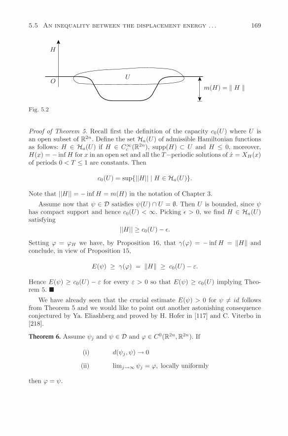
5.5 An inequality between the displacement energy . . . 169
H
OU
m(H) = ‖ H ‖
Fig. 5.2
Proof of Theorem 5. Recall first the definition of the capacity c0(U) where U isan open subset of R
2n. Define the set Ha(U) of admissible Hamiltonian functionsas follows: H ∈ Ha(U) if H ∈ C∞
c (R2n), supp(H) ⊂ U and H ≤ 0, moreover,H(x) = − inf H for x in an open set and all the T−periodic solutions of x = XH(x)of periods 0 < T ≤ 1 are constants. Then
c0(U) = sup||H|| | H ∈ Ha(U).
Note that ||H|| = − inf H = m(H) in the notation of Chapter 3.
Assume now that ψ ∈ D satisfies ψ(U) ∩ U = ∅. Then U is bounded, since ψhas compact support and hence c0(U) < ∞. Picking ε > 0, we find H ∈ Ha(U)satisfying
||H|| ≥ c0(U) − ε.
Setting ϕ = ϕH we have, by Proposition 16, that γ(ϕ) = − inf H = ‖H‖ andconclude, in view of Proposition 15,
E(ψ) ≥ γ(ϕ) = ‖H‖ ≥ c0(U) − ε.
Hence E(ψ) ≥ c0(U) − ε for every ε > 0 so that E(ψ) ≥ c0(U) implying Theo-rem 5.
We have already seen that the crucial estimate E(ψ) > 0 for ψ = id followsfrom Theorem 5 and we would like to point out another astonishing consequenceconjectured by Ya. Eliashberg and proved by H. Hofer in [117] and C. Viterbo in[218].
Theorem 6. Assume ψj and ψ ∈ D and ϕ ∈ C0(R2n, R2n). If
(i) d(ψj , ψ) → 0
(ii) limj→∞ ψj = ϕ, locally uniformly
then ϕ = ψ.
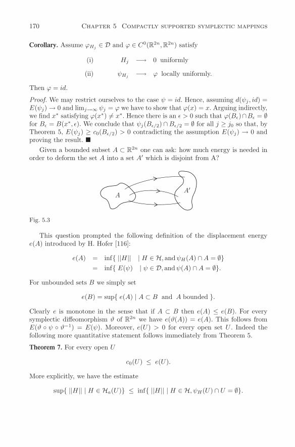
170 Chapter 5 Compactly supported symplectic mappings
Corollary. Assume ϕHj∈ D and ϕ ∈ C0(R2n, R2n) satisfy
(i) Hj −→ 0 uniformly
(ii) ψHj−→ ϕ locally uniformly.
Then ϕ = id.
Proof. We may restrict ourselves to the case ψ = id. Hence, assuming d(ψj , id) =E(ψj) → 0 and limj→∞ ψj = ϕ we have to show that ϕ(x) = x. Arguing indirectly,we find x∗ satisfying ϕ(x∗) = x∗. Hence there is an ε > 0 such that ϕ(Bε)∩Bε = ∅for Bε = B(x∗, ε). We conclude that ψj(Bε/2) ∩Bε/2 = ∅ for all j ≥ j0 so that, byTheorem 5, E(ψj) ≥ c0(Bε/2) > 0 contradicting the assumption E(ψj) → 0 andproving the result.
Given a bounded subset A ⊂ R2n one can ask: how much energy is needed in
order to deform the set A into a set A′ which is disjoint from A?
AA′
Fig. 5.3
This question prompted the following definition of the displacement energye(A) introduced by H. Hofer [116]:
e(A) = inf ||H|| | H ∈ H, and ψH(A) ∩ A = ∅= inf E(ψ) | ψ ∈ D, and ψ(A) ∩ A = ∅.
For unbounded sets B we simply set
e(B) = sup e(A) | A ⊂ B and A bounded .
Clearly e is monotone in the sense that if A ⊂ B then e(A) ≤ e(B). For everysymplectic diffeomorphism ϑ of R
2n we have e(ϑ(A)) = e(A). This follows fromE(ϑ ψ ϑ−1) = E(ψ). Moreover, e(U) > 0 for every open set U . Indeed thefollowing more quantitative statement follows immediately from Theorem 5.
Theorem 7. For every open U
c0(U) ≤ e(U).
More explicitly, we have the estimate
sup ||H|| | H ∈ Ha(U) ≤ inf ||H|| | H ∈ H, ψH(U) ∩ U = ∅.
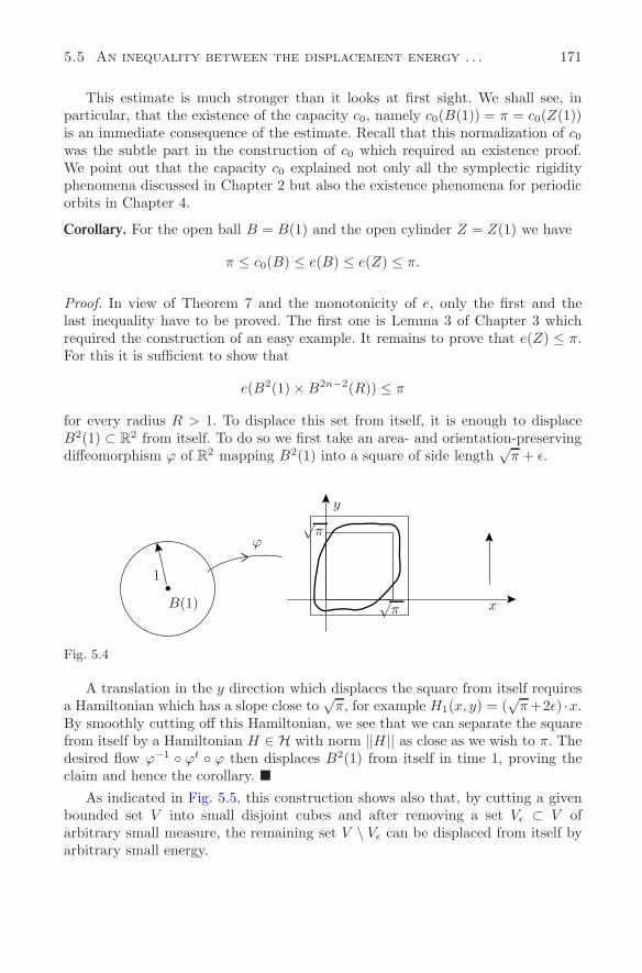
5.5 An inequality between the displacement energy . . . 171
This estimate is much stronger than it looks at first sight. We shall see, inparticular, that the existence of the capacity c0, namely c0(B(1)) = π = c0(Z(1))is an immediate consequence of the estimate. Recall that this normalization of c0
was the subtle part in the construction of c0 which required an existence proof.We point out that the capacity c0 explained not only all the symplectic rigidityphenomena discussed in Chapter 2 but also the existence phenomena for periodicorbits in Chapter 4.
Corollary. For the open ball B = B(1) and the open cylinder Z = Z(1) we have
π ≤ c0(B) ≤ e(B) ≤ e(Z) ≤ π.
Proof. In view of Theorem 7 and the monotonicity of e, only the first and thelast inequality have to be proved. The first one is Lemma 3 of Chapter 3 whichrequired the construction of an easy example. It remains to prove that e(Z) ≤ π.For this it is sufficient to show that
e(B2(1) × B2n−2(R)) ≤ π
for every radius R > 1. To displace this set from itself, it is enough to displaceB2(1) ⊂ R
2 from itself. To do so we first take an area- and orientation-preservingdiffeomorphism ϕ of R
2 mapping B2(1) into a square of side length√
π + ε.
1
B(1)
ϕ
x
y
√π
√π
Fig. 5.4
A translation in the y direction which displaces the square from itself requiresa Hamiltonian which has a slope close to
√π, for example H1(x, y) = (
√π+2ε) ·x.
By smoothly cutting off this Hamiltonian, we see that we can separate the squarefrom itself by a Hamiltonian H ∈ H with norm ||H|| as close as we wish to π. Thedesired flow ϕ−1 ϕt ϕ then displaces B2(1) from itself in time 1, proving theclaim and hence the corollary.
As indicated in Fig. 5.5, this construction shows also that, by cutting a givenbounded set V into small disjoint cubes and after removing a set Vε ⊂ V ofarbitrary small measure, the remaining set V \ Vε can be displaced from itself byarbitrary small energy.
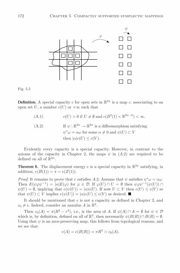
172 Chapter 5 Compactly supported symplectic mappings
ϕ
ψ
Fig. 5.5
Definition. A special capacity c for open sets in R2n is a map c, associating to an
open set U , a number c(U) or +∞ such that
(A.1) c(U) > 0 if U = ∅ and c(B2(1) × R2n−2) < ∞.
(A.2) If ψ : R2n → R
2n is a diffeomorphism satisfyingψ∗ω = αω for some α = 0 and ψ(U) ⊂ V
then |α|c(U) ≤ c(V ).
Evidently every capacity is a special capacity. However, in contrast to theaxioms of the capacity in Chapter 2, the maps ψ in (A.2) are required to bedefined on all of R
2n.
Theorem 8. The displacement energy e is a special capacity in R2n satisfying, in
addition, e(B(1)) = π = e(Z(1)).
Proof. It remains to prove that e satisfies A.2. Assume that ψ satisfies ψ∗ω = αω.Then E(ψϕψ−1) = |α|E(ϕ) for ϕ ∈ D. If ϕ(U) ∩ U = ∅ then ψϕψ−1(ψ(U)) ∩ψ(U) = ∅, implying that e(ψ(U)) = |α|e(U). If now U ⊂ V then e(U) ≤ e(V ) sothat ψ(U) ⊂ V implies e(ψ(U)) = |α|e(U) ≤ e(V ) as desired.
It should be mentioned that e is not a capacity as defined in Chapter 2, andc0 = e. Indeed, consider an annulus A in R
2.
Then c0(A) = π(R2 − r2), i.e., is the area of A. If ψ(A) ∩ A = ∅ for ψ ∈ Dwhich is, by definition, defined on all of R
2, then necessarily ψ(B(R))∩B(R) = ∅.Using that ψ is an area-preserving map, this follows from topological reasons, andwe see that
e(A) = e(B(R)) = πR2 > c0(A).
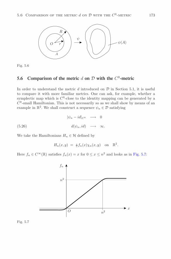
5.6 Comparison of the metric d on D with the C0-metric 173
O r
R
ψψ(A)
A
Fig. 5.6
5.6 Comparison of the metric d on D with the C0-metric
In order to understand the metric d introduced on D in Section 5.1, it is usefulto compare it with more familiar metrics. One can ask, for example, whether asymplectic map which is C0-close to the identity mapping can be generated by aC0-small Hamiltonian. This is not necessarily so as we shall show by means of anexample in R
2. We shall construct a sequence ψn ∈ D satisfying
|ψn − id|C0 −→ 0
d(ψn, id) −→ ∞.(5.26)
We take the Hamiltonians Hn ∈ H defined by
Hn(x, y) = 1nfn(x)χn(x, y) on R
2.
Here fn ∈ C∞(R) satisfies fn(x) = x for 0 ≤ x ≤ n2 and looks as in Fig. 5.7:
fn
n2
O n2x
Fig. 5.7
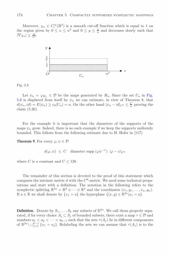
174 Chapter 5 Compactly supported symplectic mappings
Moreover, χn ∈ C∞c (R2) is a smooth cut-off function which is equal to 1 on
the region given by 0 ≤ x ≤ n2 and 0 ≤ y ≤ 2n
and decreases slowly such that|∇χn| ≤ 1
n2 .
y
2n1n
O Unn2
x
Fig. 5.8
Let ψn = ϕHn∈ D be the maps generated by Hn. Since the set Un in Fig.
5.8 is displaced from itself by ψn we can estimate, in view of Theorem 8, thatd(ψn, id) = E(ψn) ≥ c0(Un) = n. On the other hand |ψn − id|C0 ≤ C
n proving theclaim (5.26).
For the example it is important that the diameters of the supports of themaps ψn grow. Indeed, there is no such example if we keep the supports uniformlybounded. This follows from the following estimate due to H. Hofer in [117]:
Theorem 9. For every ϕ,ψ ∈ D
d(ϕ,ψ) ≤ C diameter supp (ϕψ−1) |ϕ − ψ|C0
where C is a constant and C ≤ 128.
The remainder of this section is devoted to the proof of this statement whichcompares the intrinsic metric d with the C0-metric. We need some technical prepa-rations and start with a definition. The notation in the following refers to thesymplectic splitting R
2n = R2 ⊕ · · · ⊕ R
2 and the coordinates (x1, y1, . . . , xn, yn).If a ∈ R we shall denote by x1 = a the hyperplane (x, y) ∈ R
2n|x1 = a.
Definition. Denote by S1, . . . , Sk any subsets of R2n. We call them properly sepa-
rated, if for every choice Aj ⊂ Sj of bounded subsets, there exist a map τ ∈ D andnumbers a1 < a2 < · · · < ak−1 such that the sets τ(Aj) lie in different componentsof R
2n\ ∪k−1j=1 x1 = aj. Relabeling the sets we can assume that τ(Aj) is to the
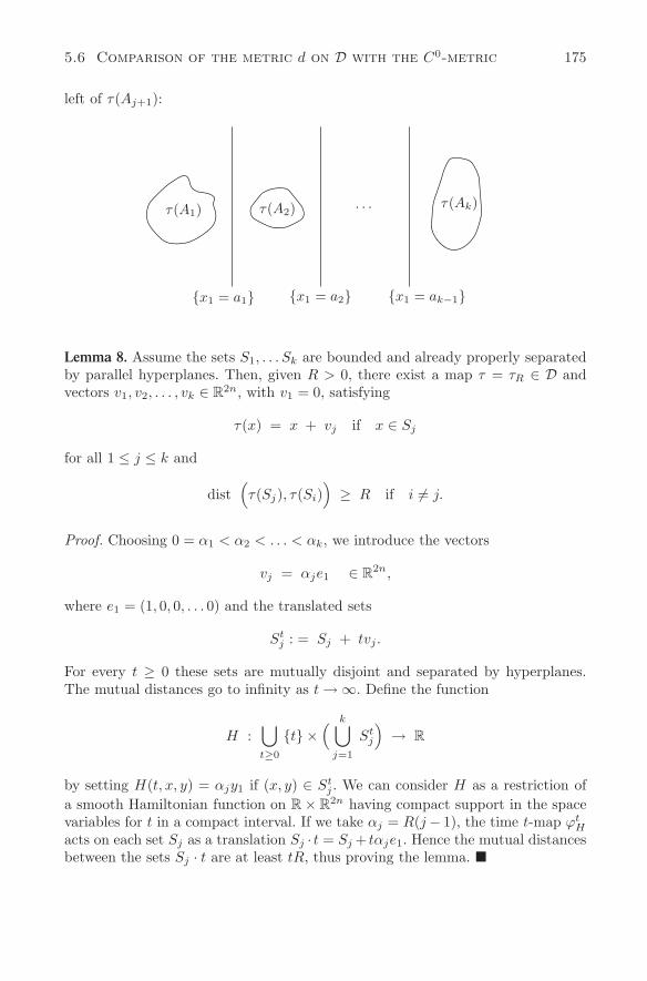
5.6 Comparison of the metric d on D with the C0-metric 175
left of τ(Aj+1):
· · ·
x1 = a1 x1 = a2 x1 = ak−1
τ(A1) τ(A2) τ(Ak)
Lemma 8. Assume the sets S1, . . . Sk are bounded and already properly separatedby parallel hyperplanes. Then, given R > 0, there exist a map τ = τR ∈ D andvectors v1, v2, . . . , vk ∈ R
2n, with v1 = 0, satisfying
τ(x) = x + vj if x ∈ Sj
for all 1 ≤ j ≤ k and
dist(τ(Sj), τ(Si)
)≥ R if i = j.
Proof. Choosing 0 = α1 < α2 < . . . < αk, we introduce the vectors
vj = αje1 ∈ R2n,
where e1 = (1, 0, 0, . . . 0) and the translated sets
Stj : = Sj + tvj.
For every t ≥ 0 these sets are mutually disjoint and separated by hyperplanes.The mutual distances go to infinity as t → ∞. Define the function
H :⋃t≥0
t ×( k⋃
j=1
Stj
)→ R
by setting H(t, x, y) = αjy1 if (x, y) ∈ Stj . We can consider H as a restriction of
a smooth Hamiltonian function on R × R2n having compact support in the space
variables for t in a compact interval. If we take αj = R(j − 1), the time t-map ϕtH
acts on each set Sj as a translation Sj · t = Sj + tαje1. Hence the mutual distancesbetween the sets Sj · t are at least tR, thus proving the lemma.
176 Chapter 5 Compactly supported symplectic mappings
Lemma 9. Assume ψ1, ψ2, . . . , ψk ∈ D have properly separated supports. Then
E(ψ1ψ2 · · ·ψk) ≤ 2 maxj
E(ψj).
Note that these maps necessarily commute.
Proof. Since the energy E is invariant under conjugation we may assume thatwe already have the supports of ψj separated by parallel hyperplanes. A prioriwe cannot assume that the generating Hamiltonians have disjoint supports. We,therefore, use a trick. Let ψj = ϕHj
and denote the support by Sj = supp (ψj).Choose R > 0 such that
supp(Hj) ⊂ [0, 1] × BR(x∗j )
where x∗j ∈ Sj . Now choose vectors vj such that the sets BR(Sj +vj) are disjoint. If
τ ∈ D is the map associated to the Sj guaranteed by Lemma 8, we set ψj = τψjτ−1
and findE(ψ1ψ2 · · ·ψk) = E(ψ1ψ2 . . . ψk).
By construction, supp(ψj) = τ(Sj) = Sj + vj. Observe now that miraculously
ψj(x) = τψjτ−1(x) = ψj(x − vj) + vj = τjψjτ
−1j (x)
for all x ∈ R2n, with the translation τj(x) = x + vj . Therefore, in view of the
transformation law of Hamiltonian vector fields,
ψj = ϕHjwith Hj(t, x) = Hj(t, x − vj).
By construction, supp(Hj) are now mutually disjoint and hence
ψ1ψ2 · · · ψk = ϕH
with H = H1 + H2 + · · · + Hk. Given ε > 0, we choose Hj such that ‖Hj‖ ≤E(ψj) + ε, so that
E(ψ1ψ2 · · ·ψk) = E(ϕH) ≤ ‖H‖.By definition,
‖H‖ =
1∫
0
(sup
xHt − inf
xHt
)dt,
and since the supports of Hj are disjoint we have
‖H‖ ≤ 2 maxj
1∫
0
(sup
xHj − inf
xHj
)dt = 2 max
j‖Hj‖ ≤ 2 max
jE(ψj) + 2ε.
This holds for every ε > 0 and the lemma is proved.
5.6 Comparison of the metric d on D with the C0-metric 177
It is useful for the following to introduce a refinement of the displacementenergy. If S ⊂ R
2n is any subset we define the proper displacement energy ep(S)as
ep(S) = infa > 0∣∣∣ for every bounded subset A ⊂ S
there exists ψ ∈ D satisfying E(ψ) ≤ a and
A and ψ(A) are properly separated
.
One verifies, as in the previous section, that ep is a special capacity for sets inR
2n which satisfies, in addition, ep(B(1)) = π = ep(Z(1)). It is an astonishingobservation that the energy of a mapping ψ ∈ D can be estimated through theproper displacement energy of the smallest support needed in order to generatethe map by a Hamiltonian. This was discovered by J.C. Sikorav in [198]:
Theorem 10. (J.C. Sikorav) If H ∈ H satisfies supp(H) ⊂ [0, 1] × U , then
E(ϕH) ≤ 16 ep(U).
Proof. Denote by ϕtH the time evolution of the map ϕH . Given ε > 0, we take N
so large that the maps ψk defined by
ψk = ϕtk
H , with tk =k
N, 0 ≤ k ≤ N
satisfyψ0 = id , ψN = ϕH
supp (ψk) ⊂ S ⊂ U , 0 ≤ k ≤ N
d(ψk, ψk+1) < ε 0 ≤ k ≤ N − 1.
Here S ⊂ R2n is a bounded subset of U . By definition of ep there exists a ϕ ∈ D
such that S and ϕ(S) are properly separated and
E(ϕ) ≤ ep(S) + ε ≤ ep(U) + ε.
We next construct a distinguished sequence of mappings ϕj ∈ D for 0 ≤ j ≤2N . If j = 0, 1 we set ϕ0 = id and ϕ1 = ϕ. In order to define ϕ2, we first choose amap σ2 ∈ D as in the proof of Lemma 8 which satisfies for s ∈ S
σ2(s) = s , σ2
(ϕ(s)
)= ϕ(s) + v2
with a vector v2 ∈ R2n.
Setting ϕ2 = σ2ϕσ−12 , we have for s ∈ S that ϕ2(s) = σ2(ϕ(s)) = ϕ(s) + v2.
Similarly, we construct all the maps ϕj by
ϕj = σjϕσ−1j , 2 ≤ j ≤ 2N
178 Chapter 5 Compactly supported symplectic mappings
choosing the translation vectors vj so that the sequence Sj of sets defined by
Sj = ϕj(S), 0 ≤ j ≤ 2N
are disjoint and pairwise properly separated. Defining now the mappings αj , βk ∈D by
αj = ϕ2j−1ψjϕ−12j−1, 1 ≤ j ≤ N
βk = ϕ2kψ−1k ϕ−1
2k , 0 ≤ k ≤ N
we see thatsupp (αj) ⊂ S2j−1, 1 ≤ j ≤ N
supp (βk) ⊂ S2k, 0 ≤ k ≤ N.
By construction the supports are mutually disjoint so that any two mappingsamong α1, . . . , αN , β0, β1 . . . βN commute. Since βN = ϕ2NϕHϕ−1
2N and β0 = id wecan use the commutativity of the maps and compute
E(ϕH ) = E(βN ) = E(βN (
N−1∏k=0
αk+1 βk)(N−1∏k=0
αk+1 βk)−1)
= E((
N∏k=1
αkβk)(N−1∏k=0
αk+1βk)−1)
≤ 2 max1≤k≤N
E(αkβk) + 2 max0≤k≤N−1
E(αk+1βk),
where we have used Lemma 9.Observing that αkβk = ϕ2k−1 (ψk ϕ−1
2k−1 ϕ2k ψ−1k )ϕ−1
2k and recalling that themaps ϕj are all conjugated to ϕ, we can estimate
E(αkβk) ≤ 4E(ϕ) ≤ 4ep(U) + 4ε.
Similarly, we find by using αk+1 βk = ϕ2k+1 (ψk+1 ψ−1k )(ψk ϕ−1
2k+1 ϕ2k ψ−1k )ϕ−1
2k
thatE(αk+1βk) ≤ 4E(ϕ) + d(ψk, ψk+1)
≤ 4ep(U) + 4ε + ε.
Summing up we have E(ϕH) ≤ 16ep(U) + 18ε, and since ε > 0 is arbitrary, theproof of Sikorav’s theorem is finished.
The following localization of Sikorav’s estimate will be crucial for the proof ofTheorem 9.
Lemma 10. Let ψ ∈ D with ψ = id and let δ > |ψ − id|C0 . For every Q ⊂ R2n
open and satisfying Q ∩ supp(ψ) = ∅, there exists a ϕ ∈ D satisfying
(i) ϕ|Q = ψ|Q
(ii) supp(ϕ) ⊂ U
(iii) E(ϕ) ≤ 16 ep(U),
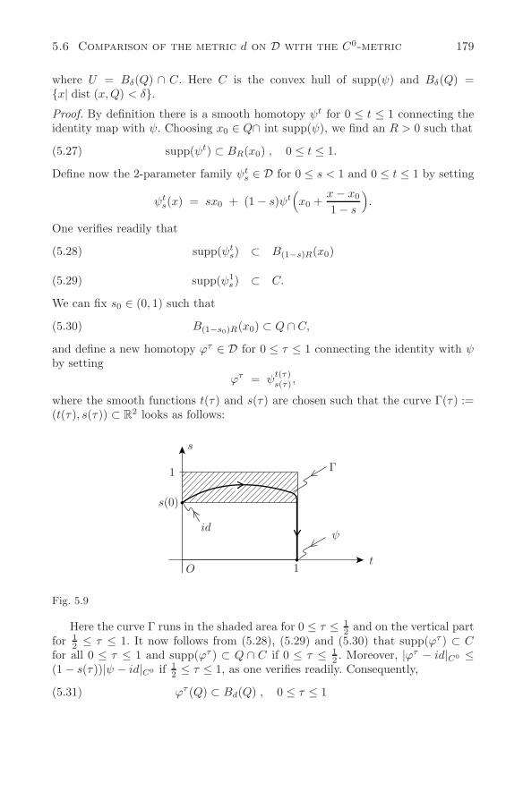
5.6 Comparison of the metric d on D with the C0-metric 179
where U = Bδ(Q) ∩ C. Here C is the convex hull of supp(ψ) and Bδ(Q) =x| dist (x,Q) < δ.Proof. By definition there is a smooth homotopy ψt for 0 ≤ t ≤ 1 connecting theidentity map with ψ. Choosing x0 ∈ Q∩ int supp(ψ), we find an R > 0 such that
supp(ψt) ⊂ BR(x0) , 0 ≤ t ≤ 1.(5.27)
Define now the 2-parameter family ψts ∈ D for 0 ≤ s < 1 and 0 ≤ t ≤ 1 by setting
ψts(x) = sx0 + (1 − s)ψt
(x0 +
x − x0
1 − s
).
One verifies readily that
supp(ψts) ⊂ B(1−s)R(x0)(5.28)
supp(ψ1s) ⊂ C.(5.29)
We can fix s0 ∈ (0, 1) such that
B(1−s0)R(x0) ⊂ Q ∩ C,(5.30)
and define a new homotopy ϕτ ∈ D for 0 ≤ τ ≤ 1 connecting the identity with ψby setting
ϕτ = ψt(τ)s(τ),
where the smooth functions t(τ) and s(τ) are chosen such that the curve Γ(τ) :=(t(τ), s(τ)) ⊂ R
2 looks as follows:
1
O
Γ
ψ
t1
id
s
s(0)
Fig. 5.9
Here the curve Γ runs in the shaded area for 0 ≤ τ ≤ 12 and on the vertical part
for 12 ≤ τ ≤ 1. It now follows from (5.28), (5.29) and (5.30) that supp(ϕτ ) ⊂ C
for all 0 ≤ τ ≤ 1 and supp(ϕτ ) ⊂ Q ∩ C if 0 ≤ τ ≤ 12 . Moreover, |ϕτ − id|C0 ≤
(1 − s(τ))|ψ − id|C0 if 12≤ τ ≤ 1, as one verifies readily. Consequently,
ϕτ (Q) ⊂ Bd(Q) , 0 ≤ τ ≤ 1(5.31)
180 Chapter 5 Compactly supported symplectic mappings
with d := |ψ− id|C0 . Since supp(ϕτ ) ⊂ C and C is convex, this homotopy is gener-ated by a Hamiltonian F ∈ H, ϕτ = ϕτ
F having its support contained in [0, 1]×C.Cutting off this function smoothly, we find a new Hamiltonian K satisfying
K∣∣∣Bd(Q) = F
∣∣∣Bd(Q)
supp(K) ⊂ [0, 1] × Bδ(Q).
In view of (5.31) we conclude for the time 1-maps that ϕK |Q = ϕF |Q = ψ|Q.Moreover, supp(K) ⊂ ([0, 1] × Bδ(Q)) ∩ supp(F ) ⊂ [0, 1] × (Bδ(Q) ∩ C) andhence supp(ϕK) ⊂ Bδ(Q)∩C. We can apply Sikorav’s theorem and find E(ϕK) ≤16ep(Bδ(Q) ∩ C). Setting ϕ = ϕK ∈ D the lemma is proved.
We shall need another consequence of Sikorav’s theorem.
Lemma 11. Assume ψ ∈ D and supp(ψ) ⊂ U . If U = (a1, a2) × (b1, b2) ⊕ R2n−2,
thenE(ψ) ≤ 16(a2 − a1)(b2 − b1).
Proof. Since U is convex we construct, as in the first part of the above proof, aHamiltonian H ∈ H satisfying supp(H) ⊂ [0, 1] × U and generating ψ = ϕH .One verifies easily, by arguing as in the proof of the Corollary to Theorem 7, thatep(U) = (a2 − a1)(b2 − b1) so that the lemma is a consequence of Sikorav’stheorem above.
Proof of Theorem 9. We consider ψ ∈ D with ψ = id and choose
δ > d = |ψ − id|C0 .
Defining the sequence aj by a0 = 0 and ak+1 = ak + 2δ, we set
Qk =[(ak − ε, ak + ε) × R
]⊕ R
2n−2
with 0 < ε < (δ − d). Since supp(ψ) is compact, the index set I ,
I =k
∣∣∣ Qk ∩ supp(ψ) = ∅
is a finite set. Choose now d < δ1 < (δ − ε). In view of the localization Lemma 10we find, for every k ∈ I, a map ϕk ∈ D satisfying
(i) ϕk|Qk = ψ |Qk
(ii) supp(ϕk) ⊂ Uk
(iii) E(ϕk) ≤ 16 ep(Uk)
5.6 Comparison of the metric d on D with the C0-metric 181
where Uk = Bδ1(Qk)∩ convex hull supp(ψ). Since Bδ1(Qk)=(ak−ε−δ1,ak +ε+δ1)×R
2n−1 and 2(ε + δ1) < 2δ, these sets are properly separated and, therefore, thesets supp(ϕk) are also. Abbreviating
R := diameter supp ψ,
we find a sequence bk ∈ R such that for every k ∈ I
Uk ⊂ (ak − ε − δ1, ak + ε + δ1) ×[bk − R
2, bk +
R
2
]⊕ R
2n−2.
Using Lemma 9 and Lemma 11 we can estimate
E( ∏
k∈I
ϕk
)≤ 2 max
k∈IE(ϕk)
≤ 2 maxk∈I
16 · 2(ε + δ1) · R
≤ 64 R · δ.(5.32)
Define ϑ = (∏k∈I
ϕk)−1. In view of (i) above and using the fact that supp(ϕk) are
properly separated, we conclude for x ∈ Qk that
ψϑ(x) = ψϕ−1k (x) = ψψ−1(x) = x.
We see that the map ψϑ is the identity map on disjoint strips, hence it leaves everygap in between invariant so that it can be written as a composition of maps havingtheir supports in the gaps. More precisely there exists a finite sequence ϕj ∈ D,with 1 ≤ j ≤ l, satisfying
ψ ϑ =l∏
j=1
ϕj ,
with supp(ϕj) properly separated and
supp(ϕj) ⊂ Uj ,
where Uj = [aj −δ +ε, aj +(δ−ε)]× [bj − R2 , bj + R
2 ]⊕R2n−2 for suitable numbers
aj and bj . We can apply Lemma 9 and Lemma 11 and find, using the estimate(5.32),
E(ψ) = E(ψϑϑ−1) ≤ E(ψϑ) + E(ϑ−1)
= E(∏
ϕj) + E(∏
ϕk)
≤ 2 · 16 · 2(δ − ε)R + 64 Rδ
≤ 128 R · δ.
182 Chapter 5 Compactly supported symplectic mappings
This holds true for every δ > d = |ψ − id|C0 , and we conclude that
E(ψ) ≤ 128 R |ψ − id|C0 ,
where R = diameter supp(ψ). Observing that |ϕψ−1−id|C0 = |ϕ−ψ|C0 , we finallyarrive at the desired estimate
d(ϕ,ψ) = E(ϕ ψ−1) ≤ 128 diameter supp(ϕ ψ−1) |ϕ − ψ|C0 ,
and the proof of Theorem 9 is finished. Finally, we shall complete the proof of Theorem 1 by proving the estimate
E(ψ) ≤ 16 infπr2 | there is a ϕ ∈ D with supp (ϕψϕ−1) ⊂ Z(r) ,(5.33)
for every ψ ∈ D. Given ε > 0, we pick a map ϑ ∈ D and R > 0 satisfyingsupp(ϑψϑ−1) ⊂ Z(R) and
πR2 − ε ≤ infπr2 | there is a ϕ ∈ D with supp(ϕψϕ−1) ⊂ Z(r).
Since E(ψ) = E(ϑψϑ−1) we may assume without loss of generality that supp(ψ) ⊂Z(R). Choosing now H ∈ H with ψH = ψ, we consider the corresponding arct → ψt and define for s > 0
ψst (x) = sψt(
1sx).
For a suitable function t → s(t) we find an arc t → ψs(t)t = ψt which is generated
by a Hamiltonian function K ∈ H satisfying supp(K) ⊂ [0, 1]×Z(R) and ψ1 = ψ.Therefore, in view of Sikorav’s estimate
E(ψ) ≤ 16πR2 ,
using that the proper displacement energy of Z(R) is equal to πR2. Since ε > 0 wasarbitrarily chosen the announced estimate (5.33) follows and the proof of Theorem1 is finally completed.
5.7 Fixed points and geodesics on D
A symplectic diffeomorphism ϕ ∈ D possesses, as we have demonstrated, a dis-tinguished fixed point x = ϕ(x) guaranteed by the minimax principle. Its actionsatisfies A(x, ϕ) = γ(ϕ). Periodic points are fixed points x = ϕN (x) of higheriterates of ϕ and we call the finite set
O(x) = x, ϕ(x), ϕ(ϕ(x)), . . . , ϕN (x) = x
the orbit of x. The following qualitative existence theorem is due to C. Viterbo[218].
5.7 Fixed points and geodesics on D 183
Theorem 11. Every ϕ ∈ D− \ id possesses infinitely many periodic points xj =ϕj(xj) having positive actions
A(xj , ϕj) ≥ γ(ϕ) > 0
and disjoint orbitsO(xj) ∩ O(xk) = ∅, k = j.
The statement also holds if ϕ ∈ D+ \ id. Actually, by using his homologicalversion of a special capacity in R
2n, C. Viterbo proved a more general statementassuming merely that ϕ ∈ D satisfies ϕ = id.
Proof. In view of the assumption on ϕ we find H ∈ H satisfying ϕ = ϕH and H ≤ 0with H = 0. Hence γ(ϕ) > 0 in view of Proposition 13. Since supp(H) ⊂ [0, 1]×Ufor some bounded open U , we have
0 < γ(ϕ) ≤ e(U).
Indeed, if ψ ∈ D satisfies ψ(U) ∩ U = ∅ then, in view of Proposition 15, γ(ϕ) ≤E(ψ) implying that γ(ϕ) ≤ e(U). Since ϕ ≤ id, we find, using the monotonicity ofγ, the estimate
0 < γ(ϕ) ≤ γ(ϕ2) ≤ . . . ≤ γ(ϕj) ≤ e(U)
for all the iterates of ϕ. For every j there is a fixed point xj = ϕj(xj) satisfyingγ(ϕj) = A(xj , ϕ
j) ≥ γ(ϕ) > 0, and it remains to show that infinitely many ofthem belong to disjoint periodic orbits. To see this observe that if xk = ϕl(xj) forsome l, then
γ(ϕk) = A(xk, ϕk) = lA(xj , ϕj) = lγ(ϕj),
as the computation shows, so that the theorem follows in view of the above boundfor the sequence γ(ϕj).
If the time-independent Hamiltonian function H ∈ C∞c (R2n) does not vanish
then the Hamiltonian system x = XH(x) possesses many periodic solutions lyingon regular energy surfaces of H, as we have seen in Chapter 4. Nothing is known,however, about their periods and we would like to add a qualitative existencestatement for fast periodic solutions. Recall that if H ∈ C∞
c (U) satisfies ||H|| >c0(U), then the system x = XH(x) possesses a nonconstant T -periodic solutionwhere the period is contained in the interval 0 < T ≤ 1, provided H ≤ 0 andH = inf H on an open subset. This follows immediately from the definition of thecapacity c0(U). Generalizing this statement we shall prove:
Theorem 12. Assume H ∈ C∞c (U) does not vanish. Then the Hamiltonian system
x = XH(x) has a nonconstant T -periodic solution with 0 < T ≤ T ∗, where
T ∗ >c0(U)|H|C0
.
184 Chapter 5 Compactly supported symplectic mappings
Proof. By using the arguments of Chapter 5, the proof will follow readily fromthe definition of the capacity c0. Let H+ = maxH and H− = −min H, then|H|C0 = maxH+,H−. Assume H+ ≥ H− so that H+ > 0 since H ≡ 0. Chooseε > 0 so small that T ∗(H+ − ε) > c0(U). Next choose a smooth function f : R →[0,∞] satisfying f(s) = 0 if s ≤ 0 and f(s) = H+ − ε if s ≥ H+ and moreover0 ≤ f ′(s) ≤ 1. Then define the Hamiltonian K by
K = T ∗ f H.
Since ‖K‖ > c0(U) there exists a nonconstant τ -periodic solution x(t) of
x = XK(x) = T ∗ f ′(H)XH(x)
of period 0 < τ ≤ 1. The function T ∗f ′(H(x(t))) = c is a positive constant,hence y(t) = x( 1
c t) is a nonconstant periodic solution of y = XH(y) having periodcτ ≤ T ∗. The same argument applies if H− ≥ H+ and the statement is proved.
With a smooth arc ϕt : [a, b] → D, we associate its length by defining
length(ϕ[a,b]
)=
b∫
a
[supx
Ht − infx
Ht]dt.
The function H is the unique smooth function on [a, b] × R2n of compact support
which generates the arc and which is determined by ( ddtϕ
t)(ϕt)−1(x) = J∇H(t, x)for a ≤ t ≤ b. In the metric space (D, d) we then call a smooth path ϕt : [a, b] → Da geodesic path if, locally, its length is the shortest connection of the endpoints;i.e., if
length (ϕ[t,s]) = d(ϕt, ϕs)
for all a ≤ t < s ≤ b with |t − s| sufficiently small. Examples of geodesics are theflows for time-independent Hamiltonians H ∈ C∞
c (R2n), as we shall show. In thiscase it follows from the definition that
length (ϕ[s,t]H ) = |t − s| · ||H||.
Proposition 17. If H ∈ C∞c (R2n) is independent of time, then the flow ϕt = ϕt
H isa geodesic in D which moreover satisfies
d(ϕt, ϕs) = |t − s| · ||H|| = length (ϕ[t,s])
for all t < s satisfying |t − s| < 2πh , where h := supx |Hxx|.
Proof. We recall first that a T− periodic solution of a time-independent vectorfield is necessarily a constant solution if the period is too small. Indeed assumex(t) is a T− periodic solution of x = XH(x). Normalizing the period we definey(t) = x(tT ), which solves
y = XTH(y), and y(0) = y(1).
5.7 Fixed points and geodesics on D 185
Note that for every 1-periodic loop z in R2n having mean value zero, we have the
L2- estimate ||z|| ≤ 12π
||z||. This is seen by looking at the Fourier series. Applyingthis observation to y whose mean value vanishes, we can estimate
||y|| ≤ 12π
||y|| =12π
T · ||Hxx(y(t))y|| ≤ Th
2π||y||,
which implies y = 0 if hT < 2π, so that y(t) = y(0) is a constant solution.Therefore, if hT < 2π, we conclude from Proposition 16 that E(ϕTH) = T ||H||.Hence assuming |t − s| < 2π
h , we can compute the distance as
d(ϕs, ϕt) = E((ϕs)−1 ϕt)
= E(ϕt−sH ) = E(ϕ(t−s)H) = |t − s|||H||,
as claimed in the proposition. Evidently, for autonomous Hamiltonians,
d(ϕt, id) = t||H|| = length (ϕ[0,t])
as long as ϕt admits no nontrivial fixed point. By definition, a geodesic in Dminimizes locally the length of the curve. Globally this need not be true as thefollowing example shows.
Proposition 18. For every ε > 0 there exists a geodesic path ϕt in D for 0 ≤ t ≤ 1starting at ϕ0 = id and satisfying, for all 0 ≤ t ≤ 1,
d(ϕt, id) ≤ ε and length (ϕ[0,t]) ≥ t
ε.
Proof. Pick an open neighborhood U of the origin satisfying 16e(U) < ε and choosea time-independent H ∈ C∞
c (U) with ||H|| > 1ε . Then, by Sikorav’s estimate, we
find if 0 ≤ t ≤ 1, that d(ϕt, id) = E(ϕtH) ≤ 16e(U) < ε, while length (ϕ[0,t]) =t||H|| ≥ t
ε as claimed. We see in particular that the metric space (D, d) is not a “flat” space. “Locally”
however the space (D, d) is “flat”. This has been proved recently by M. Bialyand L. Polterovich [22], who gave a complete description of a geodesic path in(D, d) which we shall describe next. In order to avoid pathologies, we consideronly smooth paths g : I → D, with I ⊂ R an interval, which are regular. Thisrequires that the Hamiltonian H : I × R
2n → R generating the path g satisfies||Ht|| = 0, for t ∈ I. Recall that Ht(x) = H(t, x) and, as above
||Ht|| = maxx
Ht(x) − minx
Ht(x) .
186 Chapter 5 Compactly supported symplectic mappings
Definition. A regular smooth path g : I → D is called a minimal geodesic if for alla, b ∈ I, with a < b,
length (g|[a,b]) = d(g(a), g(b)
).
Recall that the length is defined by
length (g|[a,b]) : =
b∫
a
||Ht||dt ,
where H ∈ H generates the path g. Consequently g : I → D is a geodesic path if forevery c ∈ I there is an interval Ic ⊂ I such that g : Ic → D is a minimal geodesic.In order to characterize geodesics in terms of their generating Hamiltonians, thefollowing concepts introduced in [22] turn out to be useful.
Definition. A smooth Hamiltonian H : I × R2n → R is called quasi-autonomous if
there exists two points x+, x− ∈ R2n satisfying
maxx
Ht(x) = H(t, x+) for all t ∈ I
minx
Ht(x) = H(t, x−) for all t ∈ I .
Correspondingly a function H on I ×R2n is called locally quasi-autonomous if, for
every c ∈ I, there is an interval Ic ⊂ I such that H is quasi-autonomous on Ic×R2n.
Special examples are of course autonomous Hamiltonians. Denote by C = C∞c (Rn)
the linear space of autonomous Hamiltonians equipped with the metric associatedto the norm ||H|| = maxH −min H. We call a smooth nonvanishing arc f : I → Ca minimal geodesic of C if for every a < b in I, we have
||f(b) − f(a)|| =
b∫
a
|| d
dsf(s)|| ds .
In this terminology a Hamiltonian H ∈ H is quasi-autonomous precisely if it isthe time derivative of a geodesic arc in C, in view of Lemma 13 below.
The following theorem extends Proposition 17 and gives a complete descriptionof geodesics on (D, d).
Theorem 13. (Bialy-Polterovich) A regular smooth path g : I → D is geodesic ifand only if it is generated by a locally quasi-autonomous Hamiltonian.
The rest of this section is devoted to the proof of this theorem. The result will bededuced from a criterion for minimal geodesics which we formulate first. Recall thatwith a map ϕ ∈ D we have associated in Section 5.2 its action spectrum σ(ϕ) =A(x, ϕ)|x ∈ Fix(ϕ). The action spectrum is a compact and nowhere dense set,as we have seen in Proposition 8. In general, it does not depend continuously on
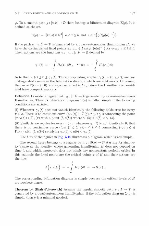
5.7 Fixed points and geodesics on D 187
ϕ. To a smooth path g : [a, b] → D there belongs a bifurcation diagram Σ(g). It isdefined as the set
Σ(g) : = (t, s) ∈ R2∣∣∣ a < t ≤ b and s ∈ σ
(g(t)g(a)−1
) .
If the path g : [a, b] → D is generated by a quasi-autonomous Hamiltonian H, wehave the distinguished fixed points x+, x− ∈ Fix(g(t)g(a)−1) for every a ≤ t ≤ b.Their actions are the functions γ+, γ− : [a, b] → R defined by
γ+(t) = −t∫
a
Ht(x−)dt , γ−(t) = −t∫
a
Ht(x+)dt .
Note that γ−(t) ≤ 0 ≤ γ+(t). The corresponding graphs Γ±(t) = (t, γ±(t)) are twodistinguished curves in the bifurcation diagram which are continuous. Of course,the curve Γ(t) = (t, 0) is always contained in Σ(g) since the Hamiltonians consid-ered have compact supports.
Definition. Consider a regular path g : [a, b] → D generated by a quasi-autonomousHamiltonian. Then its bifurcation diagram Σ(g) is called simple if the followingconditions are satisfied.
(i) Whenever γ+(t) does not vanish identically the following holds true for everyτ > a. There is no continous curve (t, u(t)) ⊂ Σ(g), τ ≤ t ≤ b connecting the point(τ, u(τ)) ∈ Γ+(τ) with a point (b, u(b)) where γ−(b) < u(b) < γ+(b).
(ii) Similarly we require for every τ > a, whenever γ−(t) is not identically 0, thatthere is no continuous curve (t, u(t)) ⊂ Σ(g), τ ≤ t ≤ b connecting (τ, u(τ)) ∈Γ−(τ) with (b, u(b)) satisfying γ−(b) < u(b) < γ+(b).
The first of the figures in Fig. 5.10 illustrates a diagram which is not simple.
The second figure belongs to a regular path g : [0, b] → D starting for simplic-ity’s sake at the identity, whose generating Hamiltonian H does not depend ontime t, and which, moreover, does not admit any nonconstant periodic orbits. Inthis example the fixed points are the critical points x of H and their actions arethe lines
A(x, g(t)
)= −
t∫
0
H(x)dt = −tH(x) .
The corresponding bifurcation diagram is simple because the critical levels of Hare nowhere dense.
Theorem 14. (Bialy-Polterovich) Assume the regular smooth path g : I → D isgenerated by a quasi-autonomous Hamiltonian. If the bifurcation diagram Σ(g) issimple, then g is a minimal geodesic.
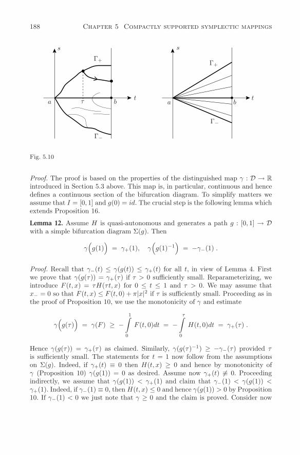
188 Chapter 5 Compactly supported symplectic mappings
a
s
τ b
Γ+
Γ−
ta
s
b
Γ+
Γ−
t
Fig. 5.10
Proof. The proof is based on the properties of the distinguished map γ : D → R
introduced in Section 5.3 above. This map is, in particular, continuous and hencedefines a continuous section of the bifurcation diagram. To simplify matters weassume that I = [0, 1] and g(0) = id. The crucial step is the following lemma whichextends Proposition 16.
Lemma 12. Assume H is quasi-autonomous and generates a path g : [0, 1] → Dwith a simple bifurcation diagram Σ(g). Then
γ(g(1)
)= γ+(1), γ
(g(1)−1
)= −γ−(1) .
Proof. Recall that γ−(t) ≤ γ(g(t)) ≤ γ+(t) for all t, in view of Lemma 4. Firstwe prove that γ(g(τ)) = γ+(τ) if τ > 0 sufficiently small. Reparameterizing, weintroduce F (t, x) = τH(τt, x) for 0 ≤ t ≤ 1 and τ > 0. We may assume thatx− = 0 so that F (t, x) ≤ F (t, 0) + π|x|2 if τ is sufficiently small. Proceeding as inthe proof of Proposition 10, we use the monotonicity of γ and estimate
γ(g(τ)
)= γ(F ) ≥ −
1∫
0
F (t, 0)dt = −τ∫
0
H(t, 0)dt = γ+(τ) .
Hence γ(g(τ)) = γ+(τ) as claimed. Similarly, γ(g(τ)−1) ≥ −γ−(τ) provided τis sufficiently small. The statements for t = 1 now follow from the assumptionson Σ(g). Indeed, if γ+(t) ≡ 0 then H(t, x) ≥ 0 and hence by monotonicity ofγ (Proposition 10) γ(g(1)) = 0 as desired. Assume now γ+(t) ≡ 0. Proceedingindirectly, we assume that γ(g(1)) < γ+(1) and claim that γ−(1) < γ(g(1)) <γ+(1). Indeed, if γ−(1) ≡ 0, then H(t, x) ≤ 0 and hence γ(g(1)) > 0 by Proposition10. If γ−(1) < 0 we just note that γ ≥ 0 and the claim is proved. Consider now
5.7 Fixed points and geodesics on D 189
the graph Γ defined by the continuous function u(t) = minγ(g(t)), γ+(t), forτ ≤ t ≤ 1. Then Γ ⊂ Σ(g) and we arrive at a contradiction to the requiredsimplicity of Σ(g). We have proved the first statement in the lemma; similarly oneobtains the second statement.
The proof of Theorem 14 follows now in view of Proposition 14; abbreviatingg(1) = ϕ we can estimate
γ+(1) − γ−(1) ≤ γ(ϕ) + γ(ϕ−1) ≤ d(id, ϕ) ≤
≤ length (g|[0,1]) = γ+(1) − γ−(1) ,
where we have used in the last equality that the Hamiltonian is quasi-autonomous.We conclude that d(id, ϕ) = length (g|[0,1]). Hence g is a minimal geodesic and theproof of Theorem 14 is completed.
A technically convenient way to describe a small neighborhood of a point ϕ ∈ Duses the linear space of generating functions which is explained in Appendix 1.Assume ϕ ∈ D is near the identity mapping and, in symplectic coordinates, givenby ϕ : (x, y) → (ξ, η) = ϕ(x, y) ∈ R
2n. Then it can implicitly be represented interms of a single function S by the relations
x = ξ + ∂∂y S(ξ, y)
η = y + ∂∂ξ S(ξ, y) ,
(5.34)
where S ∈ C∞c (R2n) is also of compact support and small in the C2-sense. Con-
versely every such function S defines by means of the formula (5.34), a symplecticmap ϕ ∈ D near the identity. We, therefore, have a mapping
Φ : S → Φ(S) ∈ D ,
defined in a small neighborhood of zero in C∞c (R2n). To an arc St(ξ, y) = S(t, ξ, y),
t ∈ I, there belongs a path g(t) = Φ(St) ∈ D for t ∈ I. It is generated by aHamiltonian H ∈ H. Its relation to St is the Hamilton-Jacobi equation
H(t, ξ, y +
∂
∂ξS(t, ξ, y)
)=
∂
∂tS(t, ξ, y) ,
which holds true in our situation for all (ξ, y) ∈ R2n. This is, of course, well-known,
and we refer to the book by C.L. Siegel and J. Moser [196]. In the linear spaceC∞
c (R2n) of generating functions we introduce the norm ||S|| := maxS − min Sand the associated metric d0(S0, S1) := ||S0 −S1||. The arc length of a smooth arcSt, a ≤ t ≤ b is, therefore, defined by
length (S[a,b]) =
b∫
a
||∂S
∂t||dt .
190 Chapter 5 Compactly supported symplectic mappings
A smooth arc St, t ∈ I is called a minimal geodesic, if for every a, b ∈ I, a < b, wehave d0(Sa, Sb) = length (S[a,b]) or, explicitly, if
||Sa − Sb|| =
b∫
a
||∂S
∂t||dt for all a < b ,
a, b ∈ I. Examples of minimal geodesics are straight lines (1 − t)Sa + tSb = St
connecting two points Sa and Sb. Lemma 13 below expresses the fact that a smootharc St is a minimal geodesic if and only if ∂S
∂t is quasi-autonomous. It will turnout that the image of a geodesic under the map Φ is a geodesic in the metricspace (D, d). Indeed we shall deduce from Theorem 14 that Φ is an isometry. Thisshows, in particular, that the metric space (D, d) is “locally flat” if one considersthe space (C∞
c (R2n), || · ||) as a “flat” space.
Theorem 15.d(Φ(S0),Φ(S1)
)= ||S0 − S1|| .
Proof. Define the arc St = (1−t)S0+tS1, 0 ≤ t ≤ 1 connecting S0 with S1. We shallprove that the path g(t) := Φ(St) is a minimal geodesic in (D, d). It connects g(0) =Φ(S0) with g(1) = Φ(S1). In order to verify the assumptions of Theorem 14 weshall prove that Σ(g) is simple and the generating Hamiltonian quasi-autonomous.Consider a fixed point (ξ, η) ∈ R
2n of g(τ)g(0)−1, i.e., g(τ)g(0)−1(ξ, η) = (ξ, η)for some 0 < τ ≤ 1 fixed. Introducing (ξ, η) = g(0)(x, y), this is equivalent to theconditions
(ξ, η) = g(τ)(x, y) = g(0)(x, y) .
Expressed in terms of the generating functions Sτ of g(τ), respectively, S0 of g(0)by means of the formula (5.34), this is equivalent to
x = ξ + ∂∂y Sτ (ξ, y) = ξ + ∂
∂y S0(ξ, y)
η = y + ∂∂ξ Sτ (ξ, y) = y + ∂
∂ξ S0(ξ, y) .
Consequently ∇Sτ (ξ, y) = ∇S0(ξ, y) and hence ∇(S0−S1)(ξ, y) = 0 and, reversingthe steps, g(t)g(0)−1(ξ, η) = (ξ, η) for all t. We have verified that the periodicsolutions of H correspond one-to-one to the critical points of the function S0 −S1
and are, moreover, all constant. From the Hamilton-Jacobi equation we deduce forthe critical points (ξ, η) = g(0)(x, y), that
H(t, ξ, y +
∂
∂ξS0(ξ, y)
)= (S1 − S0)(ξ, y) .
Hence, the Hamiltonian function is quasi-autonomous. The action of a fixed pointP = (ξ, η) which corresponds to the critical point (ξ, y) of S1 − S0 is easily com-
5.7 Fixed points and geodesics on D 191
puted:
A(P, g(t)g(0)−1
)= −
t∫0
Hs(P )ds = −t∫0
(S1 − S0)(ξ, y)ds
= −t(S1 − S0)(ξ, y) .
Since the critical values are nowhere dense, the bifurcation diagram Σ(g) is simple.We have verified for the path g(t) that the assumptions of Theorem 14 are met.Using that ||Ht|| = ||S1 − S0|| we find
d(Φ(S0),Φ(S1)
)=
1∫
0
||Ht||dt = ||S1 − S0||
and the proof of Theorem 15 is completed. In order to deduce Theorem 13 from Theorem 15, we start with two technical
observations. In order to check that a function is quasi-autonomous the followinglemma is helpful.
Lemma 13. A smooth function H : [a, b] × R2n → R of compact support is quasi-
autonomous if and only if
b∫
a
||Ht||dt = ||b∫
a
H(t, x)dt|| .
Proof. Clearly, if H is quasi-autonomous, the equation follows from the definition ofthe norm. Assuming the equality to hold we now show that H is quasi-autonomous.By definition, there exists a compact set K ⊂ R
2n containing the supports of Ht
for every t. Defining the closed sets
Kt = x ∈ K | Ht(x) = max Ht , a ≤ t ≤ b,
we have to prove that⋂
Kt = ∅, where a ≤ t ≤ b. Since K has the finite intersectionproperty it suffices to verify that Kt1 ∩ · · · ∩ KtN
= ∅ for every finite sequencet1 < t2 < · · · < tN . Arguing by contradiction, we assume Kt1 ∩ · · · ∩ KtN
= ∅.Thus we find an ε > 0 satisfying
N∑j=1
Htj(x) + ε ≤
N∑j=1
max Htjfor all x .
Consequently, by taking small intervals around the tj ’s we find an open set V ⊂[a, b] on which
∫
V
Ht(x)dt +ε
2≤
∫
V
max Htdt for all x ,
192 Chapter 5 Compactly supported symplectic mappings
and thus arrive at the contradiction
||b∫
a
Ht|| +ε
2≤
b∫
a
||Ht|| .
Arguing similarly for the minimum, the proof is completed. Lemma 14. Consider an arc St, t ∈ I = [a, b] and the corresponding arc Ht, t ∈ Igenerating the path g(t) = Φ(St) in D. Then ∂S
∂t is quasi-autonomous in I if andonly if H is quasi-autonomous in I. Moreover, in this case the distinguished pointsP± = (ξ±, η±) respectively Q± = (ξ±, y±) of min and max for H respectively∂S∂t
, are related by (5.34), the generating function being S = Sa. In additionH(t, P±) = ∂S
∂t (t,Q±) for all t ∈ I.
Proof. If H is quasi-autonomous with respect to the distinguished points P±, theng(t)g(0)−1(P±) = P± for all a ≤ t ≤ b. Hence, arguing as in the proof of Theorem15, ∇St(Q±) is independent of t and so ∇St(Q±) = ∇Sa(Q±). Consequently ∂
∂tS
is quasi-autonomous in view of the Hamilton-Jacobi equation. Conversely, if ∂S∂t
takes on its max and min at the fixed points Q±, then St − Sa also takes on itsmin and max at these points, for all t ∈ I. Hence ∇St(Q±) = ∇Sa(Q±) andconsequently g(t)g(0)−1(P±) = P±. In view of the Hamilton-Jacobi equation, thefunction H is quasi-autonomous with respect to P±. Proof of Theorem 13. The metric in (D, d) is bi-invariant and hence we may con-sider a path g(t) ∈ D near the identity g(0) = id, where t ∈ [−ε, ε] = I for asufficiently small ε > 0. It is generated by H ∈ H and g(t) = Φ(St), t ∈ I for anarc St of generating functions. We have to show that g is a minimal geodesic in(D, d) if and only if H, or equivalently ∂S
∂t (by Lemma 14), is quasi-autonomous.But by Lemma 13, ∂S
∂t is quasi-autonomous if and only if
||ε∫
−ε
∂S
∂t|| =
ε∫
−ε
||∂S
∂t|| .(5.35)
The right hand side is, in view of the Hamilton-Jacobi equation, equal toε∫
−ε
||∂S
∂t|| =
ε∫
−ε
||Ht|| = length (g|[−ε,ε]) ,
while the left hand side is equal to
||ε∫
−ε
∂S
∂t|| = ||Sε − S−ε|| = d
(g(−ε), g(ε)
),
in view of Theorem 15. Hence (5.35) holds if and only if g(t) is a minimal geodesicfor t ∈ I. The proof of Theorem 13 is completed.
Chapter 6
The Arnold conjecture, Floer homology andsymplectic homology
In the sixties V.I. Arnold announced several seminal and fruitful conjectures insymplectic topology. This chapter is devoted to his conjecture about fixed pointsof symplectic mappings which originates in questions of celestial mechanics datingback to the turn of the century. Reformulated dynamically, this conjecture givesa lower bound for the number of global forced oscillations of a time-dependentHamiltonian vector field on a compact symplectic manifold in terms of the topol-ogy of this manifold. Forced oscillations are singled out by the action principle;solutions of the conjecture gave rise to new ideas and techniques in the calculusof variations and in nonlinear elliptic systems. In particular, it prompted A. Floer1986 to the construction of his homology theory.
We shall describe in the following the history of the Arnold conjecture and startwith a proof for the special case of the standard torus T 2n in Section 6.2. Here wecan make use of the action principle in the H1/2 setting as introduced in Chapter 3.But this time the aim is to find all its critical points. Our strategy is inspired by C.Conley’s topological approach to dynamical systems: we shall study the structureof the set of all bounded solutions of the regularized gradient equation belongingto the action functional defined on the contractible loops of T 2n. This invariant setconsists of the critical points together with all their connecting orbits. This waythe study of the gradient flow in the infinite dimensional loop space is reduced tothe study of a gradient like continuous flow of a compact metric space whose restpoints are the desired critical points. It turns out that the compact space containsthe cohomology of the torus. The number of rest points is then estimated by theLjusternik-Schnirelman theory presented in Section 6.3.
A reinterpretation of the geometric ideas underlying the proof of the torus casein terms of partial differential equations will lead us in Section 6.4 to the proof ofthe Arnold conjecture for the larger class of compact symplectic manifolds (M,ω)satisfying [ω]|π2(M) = 0. In this general case there is no natural regularizationand we are forced to investigate the structure of the bounded solutions of thenot regularized gradient system. They are smooth solutions of a special systemof first order elliptic partial differential equations of Cauchy-Riemann type. Thesesolutions are related to M. Gromov’s pseudo holomorphic curves in (M,ω). Thecrucial compactness of the solution set will be established by means of an analyticaltechnique sometimes called bubbling off analysis. In order to get an insight intothe topology of the solution set we shall use an approximation procedure. Weapproximate the bounded solutions by solutions of a special elliptic boundary value
H. Hofer and E. Zehnder, Symplectic Invariants and Hamiltonian Dynamics, 193Modern Birkhäuser Classics, DOI 10.1007/978-3-0348-0104-1_6, © Springer Basel AG 2011
194 Chapter 6 The Arnold conjecture, Floer homology . . .
problem, to which we can apply Fredholm theory based on the Cauchy-Riemannoperator. Using the continuity property of the Alexander-Spanier cohomology wethen deduce the Arnold conjecture by the Ljusternik-Schnirelman theory as in thetorus case.
Assuming, in addition, all the forced oscillations to be nondegenerate, the geo-metric ideas will lead us in Section 6.5 to A. Floer’s new approach to Morse theoryand Floer homology. It makes use of an additional structure of the set of boundedsolutions of the not regularized gradient equation: namely, since M is compact,there are only finitely many nondegenerate forced oscillations and every boundedsolution of the gradient equation tends in forward and backward time asymptot-ically (exponentially) to a specific forced oscillation of the Hamiltonian system.The 1-dimensional connections determine an algebraic complex generated by theforced oscillations, its grading is defined by a Maslov-type index associated with anondegenerate forced oscillation, which plays the role of the Morse index. We shallmerely outline Floer’s beautiful ideas. A combination of Floer’s construction withour construction of the special capacity c0 of Chapter 3 results in a symplectichomology theory which, however, is not yet in its final form. It will be sketched,without proofs, in Section 6.6. The technical requirements of these theories, inparticular, the intricate transversality arguments are quite advanced and beyondthe scope of this book. Chapter 6 is, in contrast to the previous chapters, notself-contained.
6.1 The Arnold conjecture on symplectic fixed points
In his search for periodic solutions in the restricted three body problem of celestialmechanics, H. Poincare constructed an area-preserving section map of an annulusA on the energy surface. The annulus was bounded by the so-called direct andretrograde periodic orbits. It inspired him in 1912 to formulate the following the-orem [177]. It is called the last geometric theorem of Poincare announced shortlybefore his death. It was later proved by G. Birkhoff.
Theorem 1. (Poincare-Birkhoff) Every area preserving and orientation preservinghomeomorphism of an annulus A := S1 × [a, b] rotating the two boundaries inopposite directions possesses at least 2 fixed points in the interior (Fig.6.1).
The strength of this theorem is that it provides at once infinitely many peri-odic points if it is applied to the iterates, which leads to infinitely many periodicsolutions in applications, see [24]. In 1913 G. Birkhoff [23] succeeded in provingthis theorem by an ingenious but strictly two dimensional argument. Note that thetheorem is global in nature; there are no interior assumptions required on the map-ping. It is not a topological result: it is wrong if the area-preserving assumptionis dropped. S. Lefschetz, who undoubtedly would have enjoyed demonstrating toBirkhoff that the famous Poincare-Birkhoff fixed point theorem is a trivial conse-
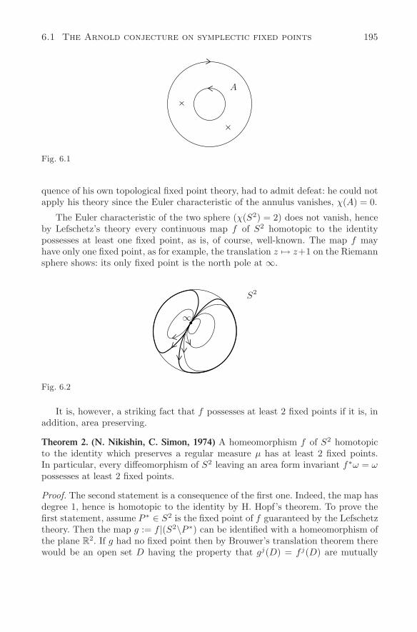
6.1 The Arnold conjecture on symplectic fixed points 195
A
Fig. 6.1
quence of his own topological fixed point theory, had to admit defeat: he could notapply his theory since the Euler characteristic of the annulus vanishes, χ(A) = 0.
The Euler characteristic of the two sphere (χ(S2) = 2) does not vanish, henceby Lefschetz’s theory every continuous map f of S2 homotopic to the identitypossesses at least one fixed point, as is, of course, well-known. The map f mayhave only one fixed point, as for example, the translation z → z+1 on the Riemannsphere shows: its only fixed point is the north pole at ∞.
∞
S2
Fig. 6.2
It is, however, a striking fact that f possesses at least 2 fixed points if it is, inaddition, area preserving.
Theorem 2. (N. Nikishin, C. Simon, 1974) A homeomorphism f of S2 homotopicto the identity which preserves a regular measure µ has at least 2 fixed points.In particular, every diffeomorphism of S2 leaving an area form invariant f∗ω = ωpossesses at least 2 fixed points.
Proof. The second statement is a consequence of the first one. Indeed, the map hasdegree 1, hence is homotopic to the identity by H. Hopf’s theorem. To prove thefirst statement, assume P ∗ ∈ S2 is the fixed point of f guaranteed by the Lefschetztheory. Then the map g := f |(S2\P ∗) can be identified with a homeomorphism ofthe plane R
2. If g had no fixed point then by Brouwer’s translation theorem therewould be an open set D having the property that gj(D) = f j(D) are mutually
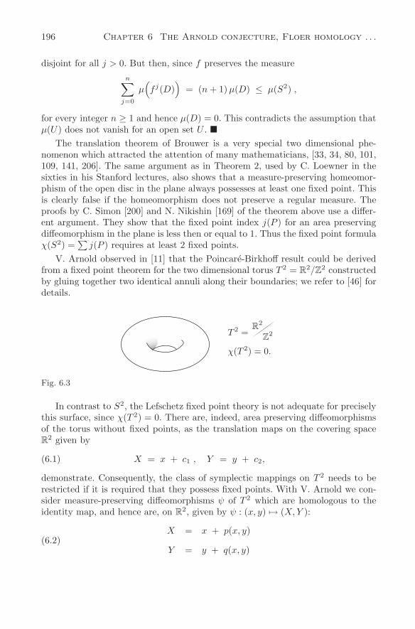
196 Chapter 6 The Arnold conjecture, Floer homology . . .
disjoint for all j > 0. But then, since f preserves the measuren∑
j=0
µ(f j(D)
)= (n + 1) µ(D) ≤ µ(S2) ,
for every integer n ≥ 1 and hence µ(D) = 0. This contradicts the assumption thatµ(U) does not vanish for an open set U .
The translation theorem of Brouwer is a very special two dimensional phe-nomenon which attracted the attention of many mathematicians, [33, 34, 80, 101,109, 141, 206]. The same argument as in Theorem 2, used by C. Loewner in thesixties in his Stanford lectures, also shows that a measure-preserving homeomor-phism of the open disc in the plane always possesses at least one fixed point. Thisis clearly false if the homeomorphism does not preserve a regular measure. Theproofs by C. Simon [200] and N. Nikishin [169] of the theorem above use a differ-ent argument. They show that the fixed point index j(P ) for an area preservingdiffeomorphism in the plane is less then or equal to 1. Thus the fixed point formulaχ(S2) =
∑j(P ) requires at least 2 fixed points.
V. Arnold observed in [11] that the Poincare-Birkhoff result could be derivedfrom a fixed point theorem for the two dimensional torus T 2 = R
2/Z2 constructed
by gluing together two identical annuli along their boundaries; we refer to [46] fordetails.
T 2 =R
2
Z2
χ(T 2) = 0.
Fig. 6.3
In contrast to S2, the Lefschetz fixed point theory is not adequate for preciselythis surface, since χ(T 2) = 0. There are, indeed, area preserving diffeomorphismsof the torus without fixed points, as the translation maps on the covering spaceR
2 given by
X = x + c1 , Y = y + c2,(6.1)
demonstrate. Consequently, the class of symplectic mappings on T 2 needs to berestricted if it is required that they possess fixed points. With V. Arnold we con-sider measure-preserving diffeomorphisms ψ of T 2 which are homologous to theidentity map, and hence are, on R
2, given by ψ : (x, y) → (X,Y ):
X = x + p(x, y)
Y = y + q(x, y)(6.2)
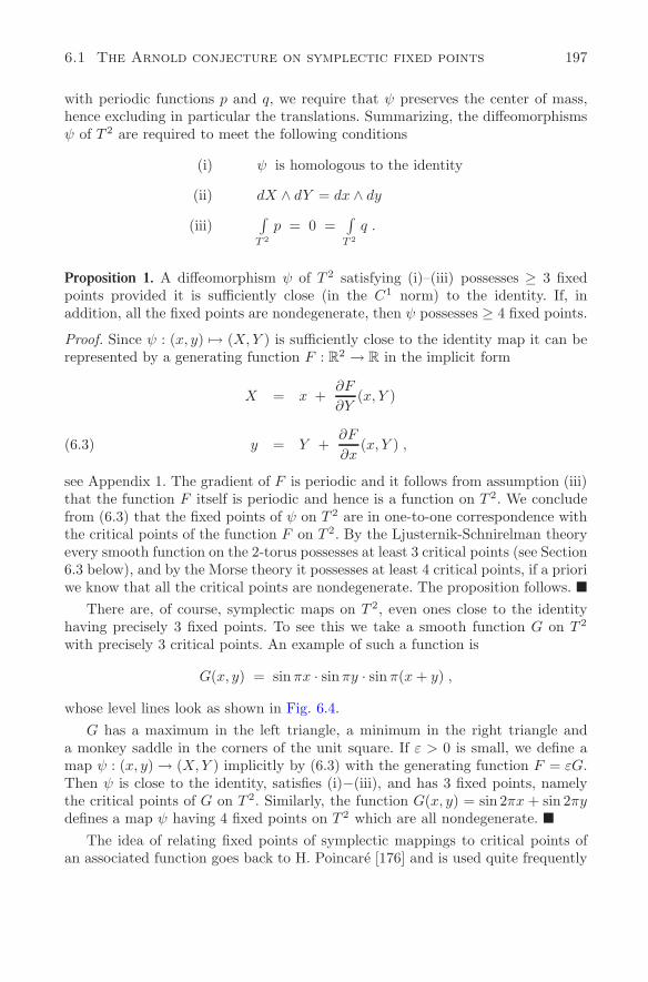
6.1 The Arnold conjecture on symplectic fixed points 197
with periodic functions p and q, we require that ψ preserves the center of mass,hence excluding in particular the translations. Summarizing, the diffeomorphismsψ of T 2 are required to meet the following conditions
(i) ψ is homologous to the identity
(ii) dX ∧ dY = dx ∧ dy
(iii)∫
T 2
p = 0 =∫
T 2
q .
Proposition 1. A diffeomorphism ψ of T 2 satisfying (i)–(iii) possesses ≥ 3 fixedpoints provided it is sufficiently close (in the C1 norm) to the identity. If, inaddition, all the fixed points are nondegenerate, then ψ possesses ≥ 4 fixed points.
Proof. Since ψ : (x, y) → (X,Y ) is sufficiently close to the identity map it can berepresented by a generating function F : R
2 → R in the implicit form
X = x +∂F
∂Y(x, Y )
y = Y +∂F
∂x(x, Y ) ,(6.3)
see Appendix 1. The gradient of F is periodic and it follows from assumption (iii)that the function F itself is periodic and hence is a function on T 2. We concludefrom (6.3) that the fixed points of ψ on T 2 are in one-to-one correspondence withthe critical points of the function F on T 2. By the Ljusternik-Schnirelman theoryevery smooth function on the 2-torus possesses at least 3 critical points (see Section6.3 below), and by the Morse theory it possesses at least 4 critical points, if a prioriwe know that all the critical points are nondegenerate. The proposition follows.
There are, of course, symplectic maps on T 2, even ones close to the identityhaving precisely 3 fixed points. To see this we take a smooth function G on T 2
with precisely 3 critical points. An example of such a function is
G(x, y) = sin πx · sinπy · sin π(x + y) ,
whose level lines look as shown in Fig. 6.4.G has a maximum in the left triangle, a minimum in the right triangle and
a monkey saddle in the corners of the unit square. If ε > 0 is small, we define amap ψ : (x, y) → (X,Y ) implicitly by (6.3) with the generating function F = εG.Then ψ is close to the identity, satisfies (i)−(iii), and has 3 fixed points, namelythe critical points of G on T 2. Similarly, the function G(x, y) = sin 2πx + sin 2πydefines a map ψ having 4 fixed points on T 2 which are all nondegenerate.
The idea of relating fixed points of symplectic mappings to critical points ofan associated function goes back to H. Poincare [176] and is used quite frequently
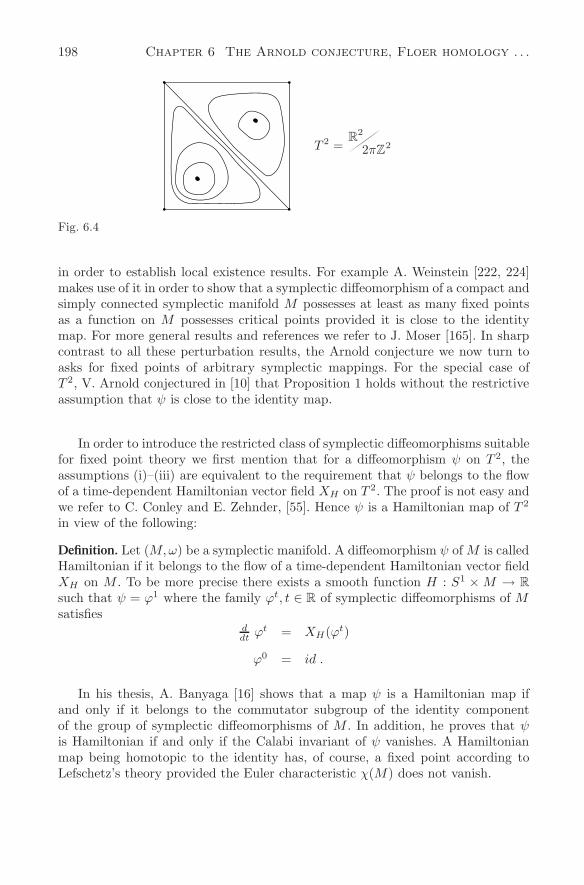
198 Chapter 6 The Arnold conjecture, Floer homology . . .
T 2 =R
2
2πZ2
Fig. 6.4
in order to establish local existence results. For example A. Weinstein [222, 224]makes use of it in order to show that a symplectic diffeomorphism of a compact andsimply connected symplectic manifold M possesses at least as many fixed pointsas a function on M possesses critical points provided it is close to the identitymap. For more general results and references we refer to J. Moser [165]. In sharpcontrast to all these perturbation results, the Arnold conjecture we now turn toasks for fixed points of arbitrary symplectic mappings. For the special case ofT 2, V. Arnold conjectured in [10] that Proposition 1 holds without the restrictiveassumption that ψ is close to the identity map.
In order to introduce the restricted class of symplectic diffeomorphisms suitablefor fixed point theory we first mention that for a diffeomorphism ψ on T 2, theassumptions (i)–(iii) are equivalent to the requirement that ψ belongs to the flowof a time-dependent Hamiltonian vector field XH on T 2. The proof is not easy andwe refer to C. Conley and E. Zehnder, [55]. Hence ψ is a Hamiltonian map of T 2
in view of the following:
Definition. Let (M,ω) be a symplectic manifold. A diffeomorphism ψ of M is calledHamiltonian if it belongs to the flow of a time-dependent Hamiltonian vector fieldXH on M . To be more precise there exists a smooth function H : S1 × M → R
such that ψ = ϕ1 where the family ϕt, t ∈ R of symplectic diffeomorphisms of Msatisfies
ddt
ϕt = XH(ϕt)
ϕ0 = id .
In his thesis, A. Banyaga [16] shows that a map ψ is a Hamiltonian map ifand only if it belongs to the commutator subgroup of the identity componentof the group of symplectic diffeomorphisms of M . In addition, he proves that ψis Hamiltonian if and only if the Calabi invariant of ψ vanishes. A Hamiltonianmap being homotopic to the identity has, of course, a fixed point according toLefschetz’s theory provided the Euler characteristic χ(M) does not vanish.
6.1 The Arnold conjecture on symplectic fixed points 199
The Arnold conjecture. Every Hamiltonian diffeomorphism ψ of a compact sym-plectic manifold (M,ω) possesses at least as many fixed points as a functionF : M → R on M possesses critical points.
In view of the Ljusternik-Schnirelman theory and the Morse theory for func-tions on M we reformulate this conjecture in the following somewhat weaker form:
# fixed points of ψ ≥ cup-length of M + 1 ,
and, if a priori all the fixed points of ψ are nondegenerate,
≥ sum of the Betti numbers of M .
Recall that a fixed point p of ψ is called nondegenerate if 1 is not an eigenvalue ofthe linearized map dψ(p) ∈ L(TpM). The cup-length of a manifold M is definedas the longest product in the cohomology ring: CL(M) = supk|∃α1, α2, . . . αk ∈H∗(M) with dim αj ≥ 1 such that α1 ∪ α2 ∪ · · · ∪ αk = 0. Let SB(M) denotethe sum of the Betti numbers βk = dim Hk(M), 0 ≤ k ≤ dim M . Introducing thePoincare polynomial
P (t,M) =dim M∑k=0
βk tk , βk = dim Hk(M)
we have SB(M) = P (1,M) and, of course, P (−1,M) = χ(M) is the Euler char-acteristic of M . In the special case of a 2n-dimensional torus T 2n these topologicalinvariants are CL(T 2n) = 2n and SB(T 2n) = 22n while χ(T 2n) = 0. In particular,for T 2 in Proposition 1 we see that 3 = CL(T 2) + 1 and 4 = SB(T 2).
We prefer to reformulate the conjecture dynamically. A Hamiltonian map ψ is,by definition, the time 1-map of the flow of the Hamiltonian equation x = XH(x)on M with a smooth function H : R × M → R periodic in time, H(t, x) =H(t + 1, x). Consequently, p is a fixed point of ψ if and only if p = x(0) is theinitial condition of a solution x(t) of the Hamiltonian equation which is periodicof period 1 and hence satisfies x(t + 1) = x(t) for all t ∈ R. Such a solution isalso called a forced oscillation. Instead of looking for fixed points of a map, we canlook as well for periodic solutions of a time-dependent Hamiltonian vector field;the Arnold conjecture formulates a universal lower bound on the number of forcedoscillations in terms of topological invariants of the symplectic manifold.
If (M,ω) is a compact symplectic manifold and H : R×M → R a smooth timeperiodic function H(t + 1, x) = H(t, x), then for the time-dependent Hamiltonianequation
x = XH(x) , x ∈ M
the following holds:
# contractible 1-periodic solutions ≥ CL(M) + 1 .
( ≥ SB(M) if all the contractible 1-periodic solutions are nondegenerate) .
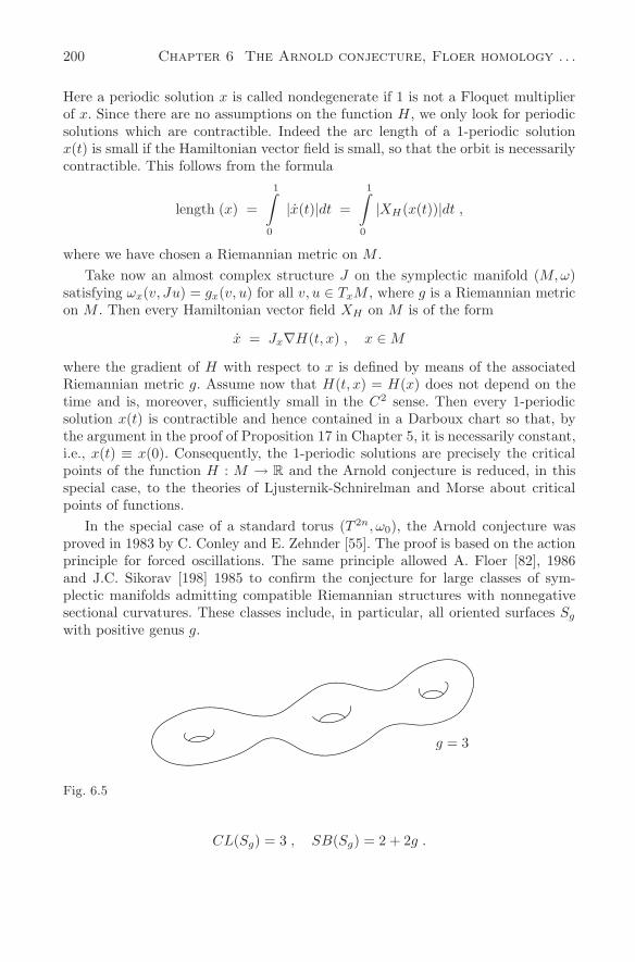
200 Chapter 6 The Arnold conjecture, Floer homology . . .
Here a periodic solution x is called nondegenerate if 1 is not a Floquet multiplierof x. Since there are no assumptions on the function H, we only look for periodicsolutions which are contractible. Indeed the arc length of a 1-periodic solutionx(t) is small if the Hamiltonian vector field is small, so that the orbit is necessarilycontractible. This follows from the formula
length (x) =
1∫
0
|x(t)|dt =
1∫
0
|XH(x(t))|dt ,
where we have chosen a Riemannian metric on M .Take now an almost complex structure J on the symplectic manifold (M,ω)
satisfying ωx(v, Ju) = gx(v, u) for all v, u ∈ TxM , where g is a Riemannian metricon M . Then every Hamiltonian vector field XH on M is of the form
x = Jx∇H(t, x) , x ∈ M
where the gradient of H with respect to x is defined by means of the associatedRiemannian metric g. Assume now that H(t, x) = H(x) does not depend on thetime and is, moreover, sufficiently small in the C2 sense. Then every 1-periodicsolution x(t) is contractible and hence contained in a Darboux chart so that, bythe argument in the proof of Proposition 17 in Chapter 5, it is necessarily constant,i.e., x(t) ≡ x(0). Consequently, the 1-periodic solutions are precisely the criticalpoints of the function H : M → R and the Arnold conjecture is reduced, in thisspecial case, to the theories of Ljusternik-Schnirelman and Morse about criticalpoints of functions.
In the special case of a standard torus (T 2n, ω0), the Arnold conjecture wasproved in 1983 by C. Conley and E. Zehnder [55]. The proof is based on the actionprinciple for forced oscillations. The same principle allowed A. Floer [82], 1986and J.C. Sikorav [198] 1985 to confirm the conjecture for large classes of sym-plectic manifolds admitting compatible Riemannian structures with nonnegativesectional curvatures. These classes include, in particular, all oriented surfaces Sg
with positive genus g.
g = 3
Fig. 6.5
CL(Sg) = 3 , SB(Sg) = 2 + 2g .
6.1 The Arnold conjecture on symplectic fixed points 201
The earlier proofs by Ya. Eliashberg for surfaces [77] are based on differentideas and were never published. The case S2 = CP 1 was extended to higherdimensions by B. Fortune [93, 94] in 1985, who verified the conjecture for CPn
with its standard symplectic structure. Accordingly every Hamiltonian map onCPn has ≥ n + 1 fixed points. Note that in this case CL + 1 = SB = χ = n + 1,so that in the nondegenerate case the result follows already from the Lefschetztheorem. A. Weinstein pointed out in [227] 1986 that the Arnold conjecture is truefor every symplectic manifold (M,ω) if the Hamiltonian map ψ is generated bya Hamiltonian vector field sufficiently small in the C0 norm. We shall describethe more recent global results and developments in Sections 4 and 5. It will turnout, in particular, that the forced oscillations of a Hamiltonian vector field XH
on a compact symplectic manifold are more intimately related to the topology ofthe underlying manifold M than it is suggested by the conjecture above. First westudy in detail the model case of the standard torus.
Before we turn to the proofs of the Arnold conjecture in higher dimensions, wewould like to refer to some recent two dimensional results related to the Poincare-Birkhoff theorem. As mentioned before, the Arnold conjecture for the two torusT 2 may be viewed as a generalization of this theorem for diffeomorphisms andone may ask whether there is a topological analogue. Quite recently, P. Le Calvez[139] succeeded in proving that every homeomorphism of T 2 homotopic to theidentity, preserving a regular measure and preserving the center of gravity (i.e.,there is a lift to R
2 satisfying the condition (iii) in (6.2) above) possesses at leastthree fixed points. Earlier M. Flucher [91] found two fixed points by extendingtechniques and arguments of J. Franks [96, 97]. Attempts to generalize these resultsfor homeomorphisms of higher dimensional tori must fail: on Tn, n ≥ 3, there aremeasure-preserving diffeomorphisms satisfying the assumptions analogous to theT 2 case without any fixed points, see M. Flucher [91]. An interesting modificationof the Poincare-Birkhoff theorem for the annulus has been discovered by J.M.Gambaudo and P. Le Calvez [103] and, independently, by J. Franks [100]:
Theorem 3. A diffeomorphism of the closed annulus A = R/Z × [0, 1], isotopic tothe identity and preserving a regular measure, possesses infinitely many periodicorbits in the interior of A, provided it has a fixed point.
This result has astonishing consequences. By introducing polar coordinates(r, ϑ) in the neighborhood of a fixed point, one can blow up the fixed point intoan invariant circle defined by r = 0. Given two fixed points on a sphere S2, oneobtains in this way a map of a closed annulus and hence deduces from Theorem 3the following:
Corollary. Consider a C2-diffeomorphism of S2 preserving the orientation andpreserving a regular measure. If it has 3 fixed points then it has infinitely manyperiodic orbits.
In view of Theorem 2 such a diffeomorphism always has at least two fixedpoints and it is sufficient to assume one of them to be hyperbolic. Indeed, the
202 Chapter 6 The Arnold conjecture, Floer homology . . .
blown up invariant circle of a hyperbolic fixed point contains 4 fixed points so thatTheorem 3 applies.
J. Franks used Theorem 3 for his breakthrough in an old problem of Rieman-nian geometry. In [25] G. Birkhoff describes a reduction of the study of the geodesicflow on a Riemannian two-sphere to the study of an area preserving annulus mapwhose periodic points correspond to the closed geodesics. He showed, for positiveGaussian curvature, that, associated to a simple closed geodesic, such a Birkhoffannulus map is defined. Franks, assuming that S2 is equipped with a Riemannianmetric having a simple closed geodesic for which the associated Birkhoff annu-lus map is defined, demonstrates, that this map has a fixed point and hence, byTheorem 3, infinitely many periodic points. If, on the other hand, a Riemannianmetric on S2 has no simple closed geodesic for which the Birkhoff annulus mapis defined, then V. Bangert [15] established infinitely many closed geodesics byvariational methods applied to the energy functional on the loop space of S2. It iswell known that every Riemann sphere possesses a simple closed geodesic. Hence,on a Riemann two-sphere there are always infinitely many closed geodesics whichare distinct as point sets.
References related to the Poincare-Birkhoff theorem and its generalizations are:[4, 35, 38, 49, 48, 61, 91, 95, 96, 97, 98, 99, 103, 109, 138, 140, 141, 139, 200, 206,143].
6.2 The model case of the torus
We shall prove the Arnold conjecture for the standard torus (T 2n, ω0), where T 2n =R
2n/Z2n and where ω0 denotes the symplectic structure induced by the standard
one from R2n. A Hamiltonian vector field on this torus depending periodically on
time is given simply by a smooth function H : R × R2n → R, (t, x) → H(t, x)
which is periodic in all its variables:
H(t + 1, x) = H(t, x) = H(t, x + j) , all j ∈ Z2n .(6.4)
The associated Hamiltonian system is represented by
x = J ∇H(t, x) , x ∈ R2n .(6.5)
A periodic solution t → x(t) = x(t + 1) ∈ R2n of (6.5) represents a contractible
periodic solution of the vector field on T 2n. In contrast, a solution of the formx(t) = jt + ξ(t), with j = 0 ∈ Z
2n and ξ(t) = ξ(t + 1) represents a 1-periodicsolution on T 2n which is not contractible. Yet, such solutions might not existon T 2n, as was explained in the previous section. We shall prove the followingqualitative existence statement for Hamiltonian flows:
6.2 The model case of the torus 203
Theorem 3. (C. Conley and E. Zehnder) Every smooth time periodic Hamiltonianvector field on the standard torus (T 2n, ω0) possesses at least 2n + 1 contractible1-periodic solutions (resp. at least 22n if all of them are nondegenerate).
We shall merely consider the first statement which does not impose any as-sumptions on the Hamiltonian on T 2n. Our proof in the following is based on theaction principle and is designed to illustrate, in the analytical framework of Chap-ter 3, some of the underlying geometric ideas which will be used for a large classof symplectic manifolds described later.
A contractible loop S1 → T 2n is the projection of a smooth loop x : S1 → R2n
represented by its Fourier expansion
x(t) =∑k∈Z
e2πk Jt xk , xk ∈ R2n .(6.6)
Two such loops x and y on R2n induce the same contractible loop on T 2n iff
x(t) − y(t) = j ∈ Z2n for all t ∈ R, so that xk = yk for k = 0 and x0 = y0 + j.
Consequently, we can identify the space of smooth contractible loops on T 2n withthe space
T 2n × E∞ ,
where E∞ := x ∈ C∞(S1, R2n)|∫ 1
0x(t)dt = 0. This space is the quotient under
the Z2n-action of the space R
2n × E∞ ∼= C∞(S1, R2n). Using the same analyticalframework as in Chapter 3, we now replace the space of smooth loops E∞ by theSobolev space
E =x ∈ H1/2(S1, R2n) |
1∫
0
x(t)dt = 0
,(6.7)
which has an orthogonal splitting E = E− ⊕ E+ according to the decomposition
x =∑k =0
e2πk Jt xk =∑k<0
+∑k>0
= x− + x+ .
We shall denote the loop space of R2n by Ω = R
2n ×E and the loop space on T 2n
by Ω = T 2n × E. The smooth action ϕ : Ω → R is defined by
ϕ(x) = a(x) − b(x) , x ∈ Ω(6.8)
where
a(x) = −12||x−||2 +
12||x+||2(6.9)
stems from the symplectic structure, and where
b(x) =
1∫
0
H(t, x(t)
)dt(6.10)
204 Chapter 6 The Arnold conjecture, Floer homology . . .
contains the given Hamiltonian H. Clearly, ϕ is invariant under the Z2n action:
ϕ(x + j) = ϕ(x), x ∈ Ω, and hence defines a smooth function on the loop spaceΩ = T 2n × E of contractible loops on the torus. We know from Chapter 3 that acritical point x ∈ Ω of ϕ,
∇ϕ(x) = 0 ,(6.11)
is actually a smooth loop. The critical points are precisely the desired contractibleperiodic solutions of (6.5) we are looking for. We recall that the gradient of ϕ inH1/2 is given by
∇ϕ(x) = −x− + x+ − b′(x) ,(6.12)
where we denote by b′(x) the gradient of b in H1/2. Also recall that b′(x) =j∗ ∇b(x), with the L2-gradient ∇b(x) = ∇H(x) ∈ L2 of b, and j∗ : L2 → H1/2
the compact operator introduced in Chapter 3. Since H is a periodic function, itsgradient on R
2n is bounded and hence b′ maps Ω into a compact subset of Ω. Inorder to find the critical points of ϕ, we shall study the quite artificial gradientflow on the loop space defined by
d
dsx = −∇ϕ(x) , x ∈ Ω .(6.13)
The solutions x(s) = x · s of this smooth ordinary differential equation exist forall times since the gradient satisfies a uniform Lipschitz estimate (see Chapter 3).They are represented by
x · s = es x− + x0 + e−sx+ − K(s, x)
K(s, x) : =s∫0
(es−τP− + P 0 + e−s+τP+
)b′(x · τ)dτ .
(6.14)
The linear operators P−, P 0 and P+ denote the orthogonal projections belongingto the splitting Ω = E0 ⊕ E− ⊕ E+, where E0 = R
2n. In order to motivate ourstrategy to find critical points, we first consider a bounded orbit of the flow. Bydefinition, such an orbit x · s satisfies
sups∈R
|ϕ(x · s)| < ∞ .(6.15)
For every T > 0,
ϕ(x · T ) − ϕ(x · (−T )
)= −
T∫
−T
|∇ϕ(x · s)|2ds .(6.16)
Since s → ϕ(x · s) is monotone the limit as T → +∞ exists in view of (6.15), sothat
∞∫
−∞
||∇ϕ(x · s)||2 ds < ∞ .(6.17)
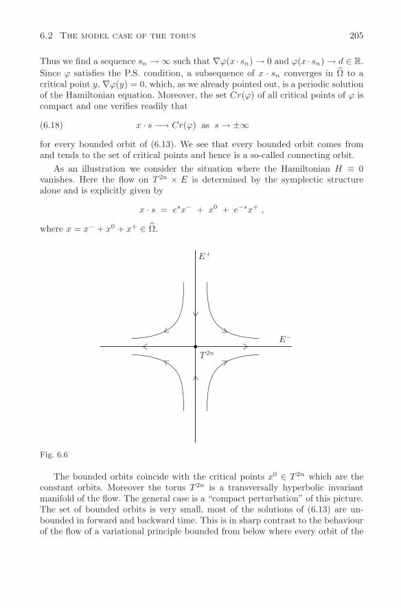
6.2 The model case of the torus 205
Thus we find a sequence sn → ∞ such that ∇ϕ(x · sn) → 0 and ϕ(x · sn) → d ∈ R.Since ϕ satisfies the P.S. condition, a subsequence of x · sn converges in Ω to acritical point y, ∇ϕ(y) = 0, which, as we already pointed out, is a periodic solutionof the Hamiltonian equation. Moreover, the set Cr(ϕ) of all critical points of ϕ iscompact and one verifies readily that
x · s −→ Cr(ϕ) as s → ±∞(6.18)
for every bounded orbit of (6.13). We see that every bounded orbit comes fromand tends to the set of critical points and hence is a so-called connecting orbit.
As an illustration we consider the situation where the Hamiltonian H ≡ 0vanishes. Here the flow on T 2n × E is determined by the symplectic structurealone and is explicitly given by
x · s = esx− + x0 + e−sx+ ,
where x = x− + x0 + x+ ∈ Ω.
E+
E−
T 2n
Fig. 6.6
The bounded orbits coincide with the critical points x0 ∈ T 2n which are theconstant orbits. Moreover the torus T 2n is a transversally hyperbolic invariantmanifold of the flow. The general case is a “compact perturbation” of this picture.The set of bounded orbits is very small, most of the solutions of (6.13) are un-bounded in forward and backward time. This is in sharp contrast to the behaviourof the flow of a variational principle bounded from below where every orbit of the
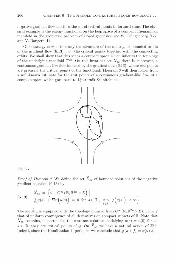
206 Chapter 6 The Arnold conjecture, Floer homology . . .
negative gradient flow tends to the set of critical points in forward time. The clas-sical example is the energy functional on the loop space of a compact Riemannianmanifold in the geometric problem of closed geodesics, see W. Klingenberg [127]and V. Bangert [14].
Our strategy now is to study the structure of the set X∞ of bounded orbitsof the gradient flow (6.13), i.e., the critical points together with the connectingorbits. We shall show that this set is a compact space which inherits the topologyof the underlying manifold T 2n. On this invariant set X∞ there is, moreover, acontinuous gradient-like flow induced by the gradient flow (6.13), whose rest pointsare precisely the critical points of the functional. Theorem 3 will then follow froma well-known estimate for the rest points of a continuous gradient-like flow of acompact space which goes back to Ljusternik-Schnirelman.
Fig. 6.7
Proof of Theorem 3. We define the set X∞ of bounded solutions of the negativegradient equation (6.13) by
X∞ =u ∈ C∞
(R, R2n × E
) ∣∣∣dds
u(s) + ∇ϕ(u(s)
)= 0 for s ∈ R , sup
s∈R
∣∣∣ϕ(u(s)
)∣∣∣ < ∞
.(6.19)
The set X∞ is equipped with the topology induced from C∞(R, R2n ×E): namelythat of uniform convergence of all derivatives on compact subsets of R. Note thatX∞ contains, in particular, the constant solutions satisfying u(s) = u(0) for alls ∈ R; they are critical points of ϕ. On X∞ we have a natural action of Z
2n.Indeed, since the Hamiltonian is periodic, we conclude that ϕ(u + j) = ϕ(u) and
6.2 The model case of the torus 207
∇ϕ(u + j) = ∇ϕ(u) for all j. In the following we shall denote by X∞ the quotientspace. It is defined by (6.20) with R
2n replaced by R2n/Z
2n = T 2n. Observe nowthat the gradient equation (6.13) is independent of time, where the role of the timeis played by the parameter s. Consequently, with s → u(s), also s → u(s + τ) isa solution for every fixed τ ∈ R. This shift in time induces a continuous R-actionon X∞ defined by
R × X∞ −→ X∞ , (τ, u) → τ ∗ u
(τ ∗ u)(s) = u(s + τ) .(6.20)
This flow has very special property: it is gradient-like with respect to the contin-uous Ljapunov function
V : X∞ −→ R defined by V (u) = ϕ(u(0)
).(6.21)
In order to prove this we have to show that the function V is strictly monotonedecreasing along the nonconstant solutions τ ∗ u of the flow (6.20). If τ > σ, then
V (τ ∗ u) − V (σ ∗ u) = ϕ(u(τ)
)− ϕ
(u(σ)
)
=τ∫σ
ddt
ϕ(u(t)
)dt
= −τ∫σ
∣∣∣∣∣∣∇ϕ
(u(t)
)∣∣∣∣∣∣2dt
(6.22)
Consequently τ → V (τ ∗ u) is monotone-decreasing. Assume now that V (τ ∗ u) =V (σ∗u) for some τ > σ. Then ϕ(u(τ)) = ϕ(u(σ)) and hence, by (6.22), ∇ϕ(u(s)) =0 for all σ ≤ s ≤ τ . Therefore, in view of the uniqueness of the solutions of thegradient equation, u(s) = u(0) for all s ∈ R and hence τ ∗ u = u for all τ ∈ R.Consequently, τ ∗ u is a constant orbit of the flow (6.20) and we have verified thatV is a Ljapunov function for the continuous flow (6.20).
Conversely, of course, if we have a constant orbit, i.e., τ ∗u = u for τ ∈ R, whichis sometimes called a rest point of the flow (6.20), then u(s) ≡ u(0) is a constantsolution of the gradient flow (6.13) and hence a critical point of our functional ϕ.
So far we do not even know whether X∞ is nonempty. In order to get an insightinto the topology of the set X∞, we define the continuous map
ρ : C∞(R, R2n × E) → R2n(6.23)
associating with u the meanvalue of the loop u(0) ∈ Ω:
ρ(u) =
1∫
0
u(0)(t)dt ∈ R2n .
With ρ : C∞(R, T 2n × E) we shall denote the map on the quotient space inducedby ρ. It turns out, and this is the crucial step in the proof of Theorem 3, that theset X∞ inherits the topology of the underlying manifold T 2n:
208 Chapter 6 The Arnold conjecture, Floer homology . . .
Theorem 4. X∞ is a compact (metric) space and
(ρ|X∞)∗ : H∗(T 2n) → H∗(X∞)(6.24)
is injective. Here and also in the following H∗ denotes the Alexander-Spaniercohomology with Z2 coefficients.
Postponing for a moment the proof of this theorem, we first observe that The-orem 3 can now be deduced from the following qualitative result of dynamicalsystems:
Theorem 5. (Ljusternik-Schnirelman) Consider a continuous gradient-like flow ona compact metric space X; then
# rest points ≥ CL(X) + 1 .
We shall prove Theorem 5 in the next section devoted to Ljusternik-Schnirelmantheory. Recalling that the critical points of ϕ are the rest points of the gradient-like flow (6.20), we conclude from Theorem 5 applied to the compact space X =X∞, that #critical points of ϕ ≥ CL(X∞) + 1. Now in view of Theorem 4,CL(X∞) ≥ CL(T 2n). Since CL(T 2n) = 2n we have established at least 2n + 1critical points of ϕ. They correspond to the desired 2n + 1 periodic solutions ofthe Hamiltonian vector field and Theorem 3 is proved.
Proof of Theorem 4. The remainder of this section is devoted to the proof of The-orem 4. In order to get an insight into the topology of the set X∞ of boundedorbits of the gradient equation (6.13) we look for smooth compact submanifoldswhich “approximate” the set X∞ and whose topology can be estimated. The de-sired cohomology of the set X∞ will then be concluded by means of the continuityproperty of the Alexander-Spanier cohomology (see Appendix 7).
If T > 0 we define a set XT consisting of solutions of a very special boundaryvalue problem for the gradient equation:
XT : =
u ∈ C∞([−T, T ], R2n × E
) ∣∣∣dds
u(s) = −∇ϕ(u(s)
), −T ≤ s ≤ T
u(−T ) ∈ R2n × E−,
u(T ) ∈ R2n × E+
.
(6.25)
We have the natural Z2n action on XT and denote by XT the quotient. It is defined
by (6.25) with R2n replaced by T 2n. We shall investigate the set XT using standard
6.2 The model case of the torus 209
methods of Fredholm theory. For this purpose we introduce the Banach spaces
B : =u ∈ C1
([−T, T ], R2n × E
) ∣∣∣u(−T ) ∈ R
2n × E−
u(T ) ∈ R2n × E+
E : =u ∈ C0
([−T, T ], R2n × E
),
(6.26)
equipped with the usual C1 respectively C0 norms. We denote by B and E thequotients under the Z
2n action. These may be identified with the Banach manifoldsdefined by (6.26) with R
2n replaced by T 2n. Now define the nonlinear smooth map
L : B −→ E , u → L(u)
L(u)(s) = dds
u(s) + ∇ϕ(u(s)
), −T ≤ s ≤ T .
(6.27)
Then L(j ∗ u) = L(u) and we shall denote by L : B → E the induced map. In thefollowing we shall use the abbreviation L(u) = u + ∇ϕ(u). Since the solutions ofthe smooth ordinary differential equation are smooth in time, we can represent thesets XT (respectively XT ) as the solution set of L(u) = 0 (respectively L(u) = 0).
XT = L−1(0) and XT = L−1(0) .(6.28)
Proposition 2. L is a nonlinear Fredholm map and the Fredholm index of thelinearized map is
ind L′(u) = 2n , u ∈ B .
Proof. From L(u) = u+u+−u−−b′(u), we obtain for the linearized map at u ∈ B
L′(u)h = h + h+ − h− − b′′(u)h ,(6.29)
and we shall show first that the linear operator b′′(u) ∈ L(B, E) is compact forevery u ∈ B. Since the derivative of a smooth compact map is compact, it issufficient to verify that the map u → b′(u) : B → E is compact, i.e., maps boundedsets into precompact sets. Fix u ∈ B; then recalling that b′(u(s)) = j∗∇b(u(s)) wecan estimate
||b′(u(s)
)− b′
(u(t)
)||1/2 =
= ||j∗(∇b(u(s)) −∇b(u(t))
)||1/2
≤ M ||∇b(u(s)) −∇b(u(t))||L2
≤ M ||H||C2 · ||u(s) − u(t)||L2
≤ C ||u(s) − u(t)||1/2 ≤ C||u||B · |t − s| ,
210 Chapter 6 The Arnold conjecture, Floer homology . . .
for a constant C depending only on the second derivative of the Hamiltonianfunction H. We conclude that b′ maps a bounded subset of B into a set in Ewhich is equi-continuous, and since, for every fixed s, the set b′(u(s))|u ∈ B =j∗∇b(u(s))|u ∈ B is precompact, we conclude by the Arzela-Ascoli theorem thatb′ maps indeed bounded sets into precompact sets.
Using now that neither the Fredholm character nor the Fredholm index of alinear operator changes if we add a compact linear operator, it is sufficient to provethat the linear operator
L0 : B → E , u → u + u+ − u−(6.30)
is Fredholm of index 2n. For its kernel one verifies readily that ker(L0) = u ∈B|u(s) = x0 ∈ R
2n consists of the constant functions with values in R2n ×0, so
that dim ker(L0) = 2n. Hence it suffices to show that L0 is surjective. Define forg ∈ E the function u by
u(s) =
s∫
−T
e−s+τ g+(τ) + g0(τ) + es−τ g−(τ)
dτ −
T∫
−T
es−τ g−(τ) dτ .
Then u satisfies the boundary conditions, i.e., u ∈ B and moreover L0(u) = g asis readily verified. This finishes the proof of the proposition. Proposition 3. L : B → E is a proper map modulo the Z
2n action, i.e., if uk is asequence satisfying L(uk) → y, then there exists a sequence jk ∈ Z
2n such thatuk + jk is precompact in B.
Proof. Recall that L = L0+b′ and set L(un) = yn. Then L0(un) = yn−b′(un). Sincedim ker (L0) < ∞ there is a continuous splitting B = B0 ⊕ B1 with B0 = ker(L0),and L0|B1 is an isomorphism of Banach spaces. Now set un = u0
n + u1n ∈ B0 ⊕ B1.
Since b′(un) and hence yn−b′(un) is bounded in E we conclude that u1n is bounded
in B. Pick a sequence jn ∈ Z2n such that u0
n + jn is bounded in R2n. Then, by the
compactness of b′, the sequence
yn − b′(un) = yn − b′(un + jn)
is precompact in B so that u1n is precompact in B. Hence after taking a subsequence
we conclude un + jn → u in B as claimed. Passing to B and E , we conclude from Proposition 2 and Proposition 3 that
the map L : B → E is a proper Fredholm map of index 2n. Similarly, the map
(L, ρ) : B → E × T 2n(6.31)
defined by u → (L(u), ρ(u)) is a proper Fredholm map having Fredholm indexequal to zero. This class of maps possesses a special degree, the Smale degree
6.2 The model case of the torus 211
mod 2, denoted by
deg2
((L, ρ), (y, m)
)(6.32)
for every point (y, m) ∈ E × T 2n. The degree “counts” mod 2 the number ofpreimages under a proper and smooth Fredholm map of index zero and is definedas follows. Assume first that x ≡ (y, m) is a regular value of F ≡ (L, ρ). If u solvesF (u) = x, the derivative F ′(u) is a surjective map, and since its index is zero, itis bijective. Thus the map F is locally one-to-one near the solutions u. Since it isproper, it follows that there are only finitely many solutions u and the degree isdefined as the number of these solutions (mod 2)
# u ∈ B | (L, ρ)(u) = (y, m) mod 2 .(6.33)
If (y, m) is not a regular value, its degree is defined by taking any regular valuenearby using the Sard-Smale theorem. That this is well-defined can be provedthe same way as for the Brouwer degree of mappings between manifolds of thesame dimensions, see J. Milnor [157]. The Smale degree mod 2 enjoys the sameuseful properties as the Brouwer degree. In particular, it is invariant under properhomotopies in the class of maps considered. For complete proofs we refer to theforthcoming book by H. Brezis and L. Nirenberg [32]. For a survey on Fredholmmaps and corresponding degrees we refer to [30].
Proposition 4.
deg2
((L, ρ), (y, m)
)= 1 for all (y, m) .
Proof. We consider the smooth homotopy of Fredholm operators Φ : [0, 1] × B →E × T 2n defined by
Φs(u) =(u + u+ − u− − s b′(u), ρ(u)
).(6.34)
Since the compactness properties proved above depend only on the C2 norm ofthe Hamiltonian function, we conclude that Φ is a proper homotopy, so that thedegree with respect to a point (y, m) is independent of s and hence
deg2
((L, ρ), (y, m)
)= deg2
(Φ0, (y, m)
),
where Φ0(u) = (u + u+ − u−, ρ(u)). Similarly we can homotope the point (y, m)to (0,m) and find that the degree is equal to
deg2
(Φ0, (0,m)
).(6.35)
We claim that the number of solutions u of Φ0(u) = (0,m) is equal to one. Indeed,if u ∈ B solves
u + u+ − u− = 0 , ρ(u) = m
u(−T ) ∈ T 2n × E− , u(+T ) ∈ T 2n × E+,
then necessarily u(s) = m ∈ T 2n is the unique solution.
212 Chapter 6 The Arnold conjecture, Floer homology . . .
Consequently, deg2 (Φ0, (0,m)) = 1 provided (0,m) is a regular value of Φ0.To see this we observe that the linearized map at u(s) = m is the linear operator
h →(h + h+ − h−,
1∫
0
h(0)(t)dt)
(6.36)
between the corresponding tangent spaces. It clearly is an isomorphism so that(0,m) is indeed a regular value and the proof is finished.
So far we know that the set XT = L−1(0) ⊂ B is compact and a smoothmanifold of dimension 2n, perhaps empty, if 0 is a regular value. Consider now thecontinuous map ρ : XT → T 2n, u → ρ(u) induced by the map ρ defined in (6.23).
Proposition 5. The map ρ : XT → T 2n induces an injective map in cohomology:
ρ∗ : H∗(T 2n) → H∗(XT ) .
In particular, the set XT is not empty.
Proof. Fix an open neighborhood U of XT in B. If y ∈ E is sufficiently close to 0,then L−1(y) ⊂ U because L is a proper map. Since, by the Sard-Smale theoremfor Fredholm maps, the set of regular points is dense we can assume, in addition,that y is a regular value of L. The aim is to prove that
(ρ|L−1(y)
)∗: H∗(T 2n) → H∗
(L−1(y)
)(6.37)
is injective. Postponing the proof we conclude from the commutativity of thediagram
U
L−1(y)
T 2n
j ρ|L−1(y) ,
ρ|U
where j denotes the inclusion map, that (ρ|U)∗ is injective as well. This holds forevery open neighborhood U of the compact set XT . Hence, using the continuityproperty of the Alexander-Spanier cohomology
H∗(XT ) = dir. lim H∗(U) ,(6.38)
where this direct limit is taken over all neighborhoods U of XT (see Appendix7). We obtain that (ρ|XT )∗ is indeed injective as claimed in the proposition. Itremains to prove the injectivity of (6.37).
6.2 The model case of the torus 213
Since y is a regular value of L, the map ρ := ρ|L−1(y) : L−1(y) → T 2n is amap between two compact manifolds of dimension 2n. We shall prove that
deg2(ρ) = 1 .(6.39)
Pick a regular value m ∈ T 2n of ρ. We claim that (y, m) is a regular value of(L, ρ). Indeed, if (L, ρ)(u) = (y, m) then L′(u) : B → E is surjective since y is,by assumption a regular value of L. Observe that ker L′(u) = T (L−1(y)). Sinceby assumption m is regular for ρ the linear map ρ′(u) : T (L−1(y)) → T (T 2n) isa bijection. Consequently the linear map (L′(u), ρ′(u)) : B → E × R
2n betweenthe corresponding tangent spaces is a bijection as well, so that (y, m) is regular asclaimed. By Proposition 4 we therefore have
1 = # (L, ρ)−1(y, m) mod 2
= # (ρ|L−1(y))−1(m) mod 2 .
Since m is regular, it follows that deg2(ρ) = 1 as claimed in (6.39).Abbreviating the compact 2n-dimensional manifold L−1(y) by M , we denote
by oM and oT the Z2 fundamental classes of M and T 2n respectively. In view of(6.39) we conclude by the homological definition of the Z2 degree (see Appendix7)
ρ∗(oM) = oT .(6.40)
We point out that on smooth compact manifolds the usual cohomology theo-ries (like the singular, Alexander-Spanier, Cech) are naturally isomorphic, see F.Warner [219]. Hence, we may consider the singular cohomology instead of theAlexander-Spanier cohomology. Then by the Poincare duality we have the isomor-phisms
Hi(M) ∩oM−→ H2n−i(M) : α → α ∩ oM .
Hi(T 2n) ∩oT−→ H2n−i(T 2n) : β → β ∩ oT .
Pick α ∈ Hi(T 2n), we have to show that ρ∗(α) = 0 implies α = 0. For this purposewe consider the composition of maps
Hi(T 2n)ρ∗
−→ Hi(M) ∩oM−→ H2n−i(M)ρ∗−→ H2n−i(T 2n)
(∩oT )−1
−→ Hi(T 2n) .
Using the naturality property of the cap product (see A. Dold [62]) and using(6.40) we compute
(∩oT )−1 ρ∗(ρ∗α) ∩ oM =
(∩oT )−1 α ∩ ρ∗(oM ) =
(∩oT )−1 α ∩ oT = α .
214 Chapter 6 The Arnold conjecture, Floer homology . . .
Consequently if ρ∗α = 0 then α = 0 proving that ρ∗ is injective. The proof ofProposition 5 is completed.
We now return to the set X∞ of bounded solutions and show that it is acompact set, which can be “approximated” by XT for T large.
Proposition 6. The space X∞ is a compact (metric) space.
Proof. If u ∈ X∞ then u(s) → Cr(ϕ) as s → ±∞. Since sup|b(u)|, u ∈ Ω < ∞it follows from the monotonicity of ϕ(u(s)) that there exists a constant C > 0satisfying
−C ≤ ϕ(u(s)
)≤ C(6.41)
for all u ∈ X∞ and all s ∈ R. Consequently the set X∞ is closed. From thevariation of constants formula (6.14) we conclude, for every T > 0
u(0)+ = e−T u(−T )+ + P+
0∫
−T
es b′(u(s)
)ds .(6.42)
Since u(s) → Cr(ϕ) as |s| → ∞, the set u(R) is bounded, and hence we conclude,as T → ∞,
u(0)+ = P+ j∗0∫
−∞
es∇b(u(s)
)ds .(6.43)
A similar formula holds for u(0)− and hence we find a compact set K ⊂ T 2n ×E such that u(0) ∈ K for all u ∈ X∞. Consequently the set u(0)|u ∈ X∞is compact. Since in the C∞-topology the solutions u depend continuously ontheir initial conditions, we conclude that X∞ is compact as well and the proof isfinished.
If u ∈ XT , then u is by definition a solution of the gradient equation for|s| ≤ T , hence it has a unique continuation to a solution u(s) for all times s ∈ R
in view of the global Lipschitz continuity of ∇ϕ. This defines an inclusion mapj : XT → C∞(R, T 2n × R) by which in the following, we can consider XT as asubset of C∞(R, T 2n × E).
Proposition 7. If U is an open neighborhood of X∞, then
XT ⊂ U
for T sufficiently large.
6.2 The model case of the torus 215
Proof. Since b maps Ω into a bounded set, there exists a constant C > 0 such that
ϕ|E− ≤ C and ϕ|E+ ≥ −C .(6.44)
Consequently, if u ∈ XT , then
−C ≤ ϕ(u(s)
)≤ C ,(6.45)
for all u ∈ XT , all |s| ≤ T and all T > 0. This follows because u(s) is a solution ofthe negative gradient equation (6.13) and hence ϕ(u(s)) is a monotone-decreasingfunction. We conclude also, that there exists a constant M > 0 such that
||u(−T )|| + ||u(T )|| ≤ M(6.46)
for u ∈ XT and all T > 0. In order to finish the proof of the proposition we argueindirectly and assume there is a sequence Tn → ∞ and a sequence un ∈ XTn
satisfying un /∈ U . We shall show that a subsequence of un(0) converges to apoint x ∈ T 2n × E through which a bounded orbit u ∈ X∞ passes. Indeed, itfollows from (6.46) together with (6.42), as in the proof of Proposition 6, thatdist (un(0)+,K+) → 0 as n → ∞, for a compact set K+. Similarly for un(0)−;hence taking a subsequence un(0) → x ∈ T 2n × E. In view of (6.45) we have−C ≤ ϕ(un(s)) ≤ C, for |s| ≤ Tn for every u where the constant C is independentof n. We conclude for the solution u(s) through x = u(0) that −C ≤ ϕ(u(s)) ≤ Cfor all s ∈ R, hence u ∈ X∞. Consequently, un ∈ U for n large in view of thetopology of C∞(R, T 2n × E) and the continuous dependence of the solutions onthe initial conditions. This contradiction proves the proposition. End of the proof of Theorem 4. In order to prove the injectivity of (ρ|X∞)∗ wetake any open neighborhood U of X∞. By Proposition 6 we have XT ⊂ U . ByProposition 5 the map (ρ|XT )∗ : H∗(T 2n) → H∗(XT ) is injective and therefore(ρ|U)∗ : H∗(T 2n) → H∗(U) is injective. This holds true for every open neighbor-hood of the compact set X∞ and, again, we conclude by the continuity of theAlexander-Spanier cohomology that (ρ|X∞)∗ : H∗(T 2n) → H∗(X∞) is injective.The proof of Theorem 4 is completed. Remarks: It should be pointed out that the torus case permits more elementaryproofs. The original proof by Conley and Zehnder in [55] is also based on theHamiltonian variational function on the loop space. However, using the linearstructure of the covering space, the very special symplectic structure ω0 and thecompactness of the torus the problem of finding critical points on the infinitedimensional loop space was reduced to the equivalent problem of finding the criticalpoints of a related functional on a finite dimensional bundle T 2n×R
N of the torus.Here the dimension N is large and depends, of course, on the Hamiltonian functionH considered. The reduction used is the so-called Ljapunov-Schmidt reduction, awell-known technique in functional analysis. The question arises whether there isan intrinsic finite dimensional approach. Indeed M. Chaperon found in [43] (1984)
216 Chapter 6 The Arnold conjecture, Floer homology . . .
another variational functional which is directly defined on a finite-dimensionalvector bundle of the torus by means of a finite sequence of generating functions.He also applied his “method of broken geodesics” to the geometric and globalintersection problem of Lagrangian submanifolds in T ∗(Tn). He showed that thezero section 0∗T n , which is diffeomorphic to Tn, can never be separated from itselfby a Hamiltonian map ϕ of T ∗(Tn). More precisely he proved that
# Tn ∩ ϕ(Tn) ≥ cup-length (Tn) + 1 ,
(≥ SB(Tn) if the intersection is transversal). This was a long-standing openquestion raised by V.I. Arnold in [9]. For modifications and further applications ofthis variational approach we refer to [41]–[44]. In this connection we also mentionA.B. Givental [105], M. Brunella [36] and Yu. V. Chekanov [47]. The related finitedimensional approach due to J.C. Sikorav [197] (1987) is based on the concept of agenerating phase function for a Lagrangian manifold. The concept appeared earlierin the theory of Fourier integral operators and we refer to L. Hormander [124]. Thiselegant approach turned out to be particularly useful for the special symplecticmanifolds (T ∗M,dλ) as demonstrated by the new proof of Hofer’s Lagrangianintersection theorem in T ∗M for general compact manifolds M generalizing thetorus case above, see [197, 136]. The result was previously discovered by H. Hofer[114] (1985). It states that
# M ∩ ϕ(M) ≥ cup-length (M) + 1 ,
for every Hamiltonian map ϕ of (T ∗M,dλ), where we have identified M with thezero section 0∗M .
In this context of finite dimensional variational arguments we should also men-tion, that in his work “Symplectic topology as the geometry of generating func-tions” [218] (1992), C. Viterbo defined symplectic capacities for Lagrangian sub-manifolds as critical values of the associated phase functions. In this way he definedthe capacities for open subsets of (R2n, ω0) by using Lagrangians which are graphsof compactly supported Hamiltonian mappings. In his 1992 lectures Ya. Eliashbergoutlined how Viterbo’s approach could be extended to an alternate constructionof the Floer-Hofer symplectic homology theory described in Section 6.6, for thespecial case of open subsets of (R2n, ω0). The details of his construction were car-ried out quite recently by L. Traynor in the preprint “Symplectic homology viagenerating functions” [212].
It seems that the finite dimensional variational approaches introduced so farare not adequate for general symplectic manifolds. For this reason we based ourproof above for the torus case on the action principle in the loop space. Our proofdemonstrates that the crucial information of the variational principle is containedin the set of bounded solutions of the artificial gradient flow. The set consists of therest points together with the connecting orbits. This observation will be relevantin Floer’s approach to the Morse theory of functionals whose gradients do not evengenerate a flow.
6.3 Gradient-like flows on compact spaces 217
6.3 Gradient-like flows on compact spaces
In the following X is a compact metric space. A flow on X is a continuous mapϕ : R × X → X : (t, x) → ϕ(t, x) = ϕt(x) satisfying
ϕt(ϕs(x)
)= ϕt+s(x)
ϕ0(x) = x(6.47)
for all t, s ∈ R and x ∈ X. An example is the flow of a differentiable vector fieldon a compact manifold. We shall use the notation
ϕt(x) = x · t
and abbreviate M · B := x · t|x ∈ M and t ∈ B for subsets M ⊂ X and B ⊂ R.If x ∈ X, then the map
t → ϕt(x) = x · t
from R into X is called the solution through the point x ∈ X. The image of thepositive (respectively negative) solution through x will be denoted by γ±(x) =x · R
± and we set γ(x) = x · R. Every point x ∈ X belongs, in view of (6.47), toprecisely one orbit γ(x). The distinguished constant solutions, characterized by
x · t = x , t ∈ R
are called rest points or fixed points of the flow, clearly γ(x) = x in this case.In order to describe the global orbit structure of a flow, it is useful to recall theconcept of the positive limit set ω(x) and the negative limit set ω∗(x) of thesolution through x ∈ X.
Definition.
ω(x) = y ∈ X∣∣∣ ∃ tj → +∞ with x · tj → y
ω∗(x) = y ∈ X∣∣∣ ∃ tj → −∞ with x · tj → y .
We summarize the well-known properties of these limit sets. Recall that X iscompact.
Proposition 8. If x ∈ X then the limit sets ω(x) and ω∗(x) are not empty, compact,connected and invariant under the flow, i.e., ω(x) ·t = ω(x) for all t ∈ R. Moreover,
x · t → ω(x) as t → +∞
x · t → ω∗(x) as t → −∞ .(6.48)
218 Chapter 6 The Arnold conjecture, Floer homology . . .
Proof. If tj → ∞ then the sequence x · tj has a convergent subsequence so thatω(x) = ∅. Assume that (6.48) does not hold; then there exists an open neigh-borhood U ⊃ ω(x) and a sequence tj → ∞ such that x · tj ∈ X\U . Hencefor a subsequence x · tj → y ∈ X\U . By definition y ∈ ω(x), in contradiction toω(x) ⊂ U . If ω(x) is not connected, then ω(x) = ω1∪ω2 for two nonempty compactand disjoint subsets ωj ⊂ X. Take disjoint open neighborhoods Uj of ωj, j = 1, 2;then, by (6.48), x · t → ω(x) and hence for t ≥ t∗, we have x · t ∈ U1 ∪ U2 andγ+(x · t) ∩ Uj = ∅ for j = 1, 2. Consequently the set γ+(x · t) is not connectedcontradicting the fact that a continuous image of an interval in R is connected.The invariance of the limit sets is an immediate consequence of the continuity ofthe flow.
We assume now, in addition, that the flow is gradient-like, i.e., we requirethat there exists a continuous function V : X → R, which is strictly monotone-decreasing along every nonconstant solution:
t > s =⇒ V (x · t) < V (x · s) .
Such a function is usually called a Ljapunov function for the flow. A well-knownspecial example is the flow generated by a smooth gradient vector field x =−∇V (x) on a compact Riemannian manifold.
Proposition 9. If the flow is gradient-like the limit sets for every solution consistsof rest points:
ω(x) and ω∗(x) ⊂ rest points ,
for every x ∈ X.
Proof. Since V (x · t) is monotone-decreasing, the limit
limt→+∞
V (x · t) = infV (x · t) | t ≥ 0 = : d
exists in R. If y ∈ ω(x) we conclude by the continuity of V that V (y) = d andhence in view of the invariance of ω(x) under the flow, V (y · t) = d for every t ∈ R.By assumption V is strictly decreasing along nonconstant solutions, hence y mustbe a rest point as claimed.
If the gradient-like flow possesses only isolated rest points, then there are onlyfinitely many of them, say x1, . . . , xN and we conclude from the proposition thatevery nonconstant solution connects two distinct rest points. Every point x ∈ Xtends under the flow to a distinguished rest point in forward and backward time.
It is not surprising that the rest points of the flow are intimately related totopological properties of X. Indeed, we shall conclude from Proposition 9 thefollowing existence statement formulated in Section 6.2 as Theorem 5.
Theorem 6. (Ljusternik-Schnirelman) For every gradient-like flow on a compactmetric space we have
# rest points ≥ cup-length (X) + 1 .
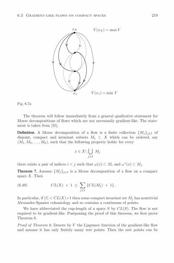
6.3 Gradient-like flows on compact spaces 219
xN
x1
V (xN ) = maxV
V (x1) = min V
Fig. 6.7a
The theorem will follow immediately from a general qualitative statement forMorse decompositions of flows which are not necessarily gradient-like. The state-ment is taken from [55].
Definition. A Morse decomposition of a flow is a finite collection Mjj∈I ofdisjoint, compact and invariant subsets Mj ⊂ X which can be ordered, say(M1,M2, . . . ,Mk), such that the following property holds: for every
x ∈ X\⋃j∈I
Mj
there exists a pair of indices i < j such that ω(x) ⊂ Mi and ω∗(x) ⊂ Mj .
Theorem 7. Assume Mjj∈I is a Morse decomposition of a flow on a compactspace X. Then
CL(X) + 1 ≤∑j∈I
CL(Mj) + 1 .(6.49)
In particular, if |I | < CL(X)+1 then some compact invariant set Mj has nontrivialAlexander-Spanier cohomology and so contains a continuum of points.
We have abbreviated the cup-length of a space S by CL(S). The flow is notrequired to be gradient-like. Postponing the proof of this theorem, we first proveTheorem 6.
Proof of Theorem 6. Denote by V the Ljapunov function of the gradient-like flowand assume it has only finitely many rest points. Then the rest points can be
220 Chapter 6 The Arnold conjecture, Floer homology . . .
ordered such that V (x1) ≤ V (x2) ≤ · · · ≤ V (xk). Since V is strictly decreasingalong the nonconstant solutions, the rest points x1, . . . , xk constitute, in view ofProposition 9, a Morse decomposition of the flow. Since CL(xj) = 0 we concludefrom Theorem 7
CL(X) + 1 ≤∑
1≤j≤k
1
so that the number of rest points must indeed be larger than or equal to CL(X)+1,thus proving Theorem 6. Proof of Theorem 7. First observe that any Morse decomposition of X can beobtained by first decomposing X into two sets, then decomposing one of these andcontinuing until the decomposition is reached. Indeed assume M1,M2, . . . ,Mk isan ordered Morse decomposition of X. Then define the subset X1 = x ∈ X|ω(x)and ω∗(x) ⊂ M1 ∪ M2 ∪ · · · ∪ Mk−1. This set is compact and invariant underthe flow so that X1,Mk constitutes an ordered Morse decomposition of X intotwo sets. Therefore one only needs to prove the theorem for decompositions intotwo sets. So let M1,M2 be an ordered Morse decomposition of X. From thedefinition we conclude that there is a compact neighborhood S1 of M1 and acompact neighborhood S2 of M2 in X satisfying S1 ∪ S2 = X and, moreover,
M1 =⋂t>0
S1 · t and M2 =⋂t>0
S2 · (−t) .
Consequently, observing that H∗(S1 · t) = H∗(S1) for every t ∈ R (similarly forS2), we conclude by the continuity property of the Alexander-Spanier cohomologythat H∗(S1) = H∗(M1) and H∗(S2) = H∗(M2). It is, therefore, sufficient to provethat c(S1) + c(S2) ≥ c(X) for S1 ∪ S2 = X, abbreviating c(S) = CL(S) + 1. Thiswill follow from the following topological observation:
Lemma 1. Let S1∪S2 ⊂ S be three compact sets. Denote by i1 : S1 → S, i2 : S2 →S and i : S1 ∪ S2 → S the inclusion maps. Assume α, β ∈ H∗(S). Then i∗1(α) = 0and i∗2(β) = 0 imply i∗(α ∪ β) = 0.
Proof of Lemma 1. Consider the following diagram:
H∗(S, S1) ⊗ H∗(S, S2)∪−→ H∗(S, S1 ∪ S2) j∗
1
j∗2
j∗
H∗(S) ⊗ H∗(S) ∪−→ H∗(S) i∗1
i∗2
i∗
H∗(S1) H∗(S2) H∗(S1 ∪ S2) .
The vertical sequences are exact. Hence if α ∈ H∗(S) satisfies i∗1(α) = 0 then thereis an α ∈ H∗(S, S1) with j∗1(α) = α. Similarly, if i∗2(β) = 0 then j∗2 (β) = α for some
6.3 Gradient-like flows on compact spaces 221
β ∈ H∗(S, S2). By the commutativity of the diagram, j∗(α∪ β) = j∗1(α)∪ j∗2 (β) =α ∪ β. and by the exactness, i∗(α ∪ β) = i∗ j∗(α ∪ β) = 0, as claimed.
Returning to the proof of Theorem 7, we assume α1, α2, . . . αl ∈ H∗(X) satisfyα1 ∪ α2 ∪ · · · ∪ αl = 0. Let the α’s be ordered so that α1 ∪ · · · ∪ αr is the longestproduct not in the kernel of i∗1. Then, by definition of the cup-length, c(S1) ≥ r+1and i∗1(α1∪· · ·∪αr∪αr+1) = 0. Since X = S1∪S2 we conclude from Lemma 1 thati∗2(αr+2 ∪ · · ·αl) = 0 and, therefore, c(S2) ≥ l − (r + 1) + 1 = l − r. Consequentlyc(S1) + c(S2) ≥ l + 1. We have shown that if X admits a nontrivial product withl factors, i.e., if c(X) ≥ l + 1, then c(S1) + c(S2) ≥ l + 1 so that Theorem 7 isproved.
We defined a gradient-like flow by a Ljapunov function which is strictly mono-tone decreasing along the nonconstant orbits of the flow. This tradition comes fromthe study of semiflows, defined only for positive time, on noncompact manifolds. Inour situation of a flow on a compact space, we could have taken a Ljapunov func-tion instead, which is strictly increasing along nonconstant orbits and we wouldhave reached the same conclusions by the same arguments. Actually, we shall makeuse of this remark in the next section, where for different reasons we consider thepositive instead of the negative gradient equation, which leads to a increasingLjapunov function. This is not relevant since our functional is bounded neitherfrom below nor from above.
Remarks: In this connection we would like to point out another useful inequalityassociated with a Morse decomposition M1, . . . ,Mk of a flow on X which is notassumed to be gradient-like. It relates dynamical invariants of the invariant setsMj to topological invariants of the space X and is due to C. Conley. Every setMj in a Morse decomposition is an isolated invariant set in the sense that it is themaximal invariant set contained in a compact neighborhood. Hence it possesses aso-called Conley-index h(Mj) which is the homotopy type of a pointed compactspace and which is determined by the flow near Mj , see C. Conley [54]. Denotingby P (t, h(Mj)) the Poincare polynomial of the pointed compact space one has∑
j
P(t, h(Mj)
)= P (t,X) + (1 + t)Q(t) ,(6.50)
P being the Poincare polynomial of the space X and Q being a power seriescontaining only nonnegative integer coefficients, for a proof we refer to [57]. ThisConley-Morse equation relates the dynamical invariants of the local invariant setsMj ⊂ X to the global topological invariant P (t,X). Consider, for example, thespecial case of a gradient flow defined by x = −∇V (x) on a compact Riemannianmanifold X. If the critical points xj of the smooth function V on X are not onlyisolated but, in addition, nondegenerate, one can show that
h (xj) =[Sm(xj)
]
is the homotopy type of a pointed sphere whose dimension m(xj) is the Morse indexof the critical point xj . Consequently P (t, h(xj)) = tm(xj) is a monomial, see
222 Chapter 6 The Arnold conjecture, Floer homology . . .
e.g. [56]. Therefore, if all the critical points of V are nondegenerate they constitutea Morse-decomposition of X and the equation (6.50) for this special flow is thefamiliar Morse equation
∑x|∇V (x)=0
tm(x) = P (t,X) + (1 + t)Q(t) .(6.51)
It relates the nature of the isolated critical points x of the differentiable functionV to those topological invariants of X which are described by the Betti numbers.
C. Conley designed his homotopy index theory in view of its invariance prop-erties under deformations. These are crucial for applications. He developed histheory for continuous flows on locally compact metric spaces. For a concise pre-sentation of this theory, we refer to D. Salamon [187]. Later on K. Rybakowski ina series of papers [184, 185, 186] extended Conley’s index theory to a restrictedclass of continuous semiflows in an infinite dimensional setting. It includes flowsgenerated by partial differential equations of parabolic type. In this more generalsetting there is also a Morse equation associated with a Morse decomposition ofan isolated compact invariant subset of the space, as has been demonstrated in[186].
6.4 Elliptic methods and symplectic fixed points
We are going to prove the Arnold conjecture for general compact symplectic man-ifolds (M,ω) satisfying [ω]|π2(M) = 0. The proof, based on the action functionalon the loop space, is inspired by the geometric ideas underlying the proof for thestandard torus in Section 6.2. But instead of looking at O.D.E. problems, we shallnow be confronted with first order elliptic systems.
For the following it is useful to first recall our approach to the torus case.The covering map R
2n → T 2n and the special symplectic structure permit byextending the action functional, originally defined on smooth contractible loops,to the Hilbert space H1/2. The gradient of the extended functional in H1/2 issmooth and can be viewed as a regularization of the L2 gradient of the action.The gradient equation on H1/2 determines a unique global flow, which has, inaddition, the necessary compactness properties. For these reasons we can find allthe critical point by using O.D.E.-methods as follows. The study of the gradientflow on the infinite dimensional space H1/2 of contractible loops can be reducedto the study of an (induced) gradient-like flow on a compact metric space X∞,an almost classical situation. The set X∞ here is the set of all bounded solutionsof the gradient flow, consisting of all the critical points of the action functionaltogether with their connecting orbits. It is, in general, not a smooth manifold.We saw that X∞ contained the topology of the underlying manifold T 2n. TheLjusternik-Schnirelman theorem, applied to the gradient-like flow on X∞, then
6.4 Elliptic methods and symplectic fixed points 223
guaranteed the required number of rest points. In order to get an insight into thetopology of the set X∞, we approximated X∞ by a set XT of solutions of a veryspecial O.D.E. boundary value problem using the special symplectic structure.Applying Fredholm theory to this boundary value problem we approximated XT
by smooth compact manifolds of dimension 2n whose topology could be estimated.By the continuity property of the Alexander-Spanier cohomology we finally foundthe desired cohomology of the set X∞.
Since the space H1/2 is not contained in C0, the loops in H1/2 have no localmeaning, and it is not easy to define H1/2 loops on a general manifold. It can bedone but the space obtained does not carry a natural manifold structure. The mainidea in the case of a general symplectic manifold (M,ω) is to replace the regularizedgradient (of the torus case) by the unregularized gradient of the action functionalon the space of smooth contractible loops of M . The associated gradient equation,however, does not determine a flow: its Cauchy initial value problem is ill posed,as we shall see. But analogous to the torus case, we can still define the set X∞ ofall bounded solutions u : R×S1 → M of the unregularized gradient equation; theyare now solutions of a system of first order elliptic partial differential equations ofCauchy-Riemann type, related to the pseudo-holomorphic curves of M. Gromov[107]. On this solution set X∞ there is, moreover, a natural R-action defining agradient-like flow. Hence, following our old strategy, we shall prove that this setof solutions is compact and contains the cohomology of the underlying manifoldM . The Arnold conjecture then follows by applying the Ljusternik-Schnirelmantheorem as in the torus case. In order to carry out this programme the O.D.E.methods of the torus case have to be replaced by P.D.E. methods. In order todetermine the topology of X∞ we shall approximate the set X∞ by the set ofsolutions XT of a distinguished elliptic boundary value problem, to which we applyFredholm theory based on the Cauchy-Riemann operator on compact surfaces. Inthis way we can approximate XT by smooth compact manifolds of dimension2n whose topology can be determined. The easy compactness arguments for thetorus case, based on O.D.E. methods, will be replaced by an intricate bubbling offanalysis based on elliptic estimates.
In order to find the crucial substitute for XT used in Section 6.2 we beginwith the analysis of the torus case T 2n = R
2n/Z2n, this time from the point
of view of the unregularized gradient. The aim is to reinterpret the approach ofSection 6.2 from a P.D.E. point of view. We recall that to a periodic functionH ∈ C∞(S1 × T 2n, R), we associated the action functional ΦH , defined on thespace of smooth contractible loops x of T 2n by
ΦH(x) =
1∫
0
12〈−Jx, x〉 − H
(t, x(t)
)dt .(6.52)
On the covering space R2n the contractible loops x are simply the smooth
functions x ∈ C∞(S1, R2n). By extending ΦH to a smooth functional ϕH on the
224 Chapter 6 The Arnold conjecture, Floer homology . . .
Hilbert space H1/2(S1, R2n) we obtained for the H1/2 gradient, which we nowdenote by ϕ′
H , the representation
ϕ′H (x) = j∗ Φ′
H(x) if x ∈ C∞(S1, R2n) .(6.53)
Here Φ′H(x) is the L2-gradient of ΦH given by
∇ΦH (x) = −Jx −∇H(t, x) ,(6.54)
and j∗ is the adjoint of the inclusion mapping j : H1/2 → L2 defined explicitly inChapter 3. We may view ϕ′
H as the regularization of the L2-gradient Φ′H by means
of the positive and compact operator j∗ on L2. Instead of the gradient equationddsx = −ϕ′
H (x) on H1/2 studied previously, we now study the unregularized equa-tion d
dsx = Φ′H(x). Observe that we now consider the positive gradient instead of
the negative one considered in Section 6.2. For indefinite functionals this is irrele-vant. However, this way we are led, as we shall see, in a natural way to the familiarCauchy-Riemann operator instead of the anti-Cauchy-Riemann operator. Settingu(t, s) = x(s)(t) for the loops at time s, we obtain the partial differential equation
∂u
∂s= −J
∂u
∂t−∇H(t, u) ,(6.55)
for a smooth function u ∈ C∞(R × S1, R2n). Abbreviating the notation in thefollowing, we write u′ = −Ju −H ′(t, u) instead of (6.55), where H ′ = ∇H standsfor the gradient of the function H in the x variable. The operator
u′ + Ju =∂u
∂s+ J
∂u
∂t(6.56)
is nothing but the well-known Cauchy-Riemann operator for maps u : R2 →
R2n. To see this it is convenient to identify R
2n with Cn as follows. We split
R2n = R
2⊕· · ·⊕R2 into symplectic subspaces R
2, having the symplectic structureω0(a, b) = 〈Ja, b〉 with the matrix J given by
J =(
0 1−1 0
).(6.57)
We identify R2 with C by means of the linear isomorphism U : C → R
2 given byz = (y + ix) → (x, y) = (Im z,Re z). On C, the complex structure is now themultiplication by i =
√−1, since
U−1J U = i ,(6.58)
and ω0 becomes ω0(z, ξ) = −Im〈z, ξ〉. Setting z = s+it ∈ C we shall view the mapu : R
2 → R2n as a map u : z → u(z) ∈ C
n so that the operator (6.56) becomesthe familiar Cauchy-Riemann operator on every copy of C,
∂u
∂s+ i
∂u
∂t= ∂u .(6.59)
6.4 Elliptic methods and symplectic fixed points 225
Similarly the operator ∂u∂s − J ∂u
∂t is, in our complex notation, the operator
∂u
∂s− i
∂u
∂t= ∂u .(6.60)
Note that for convenience we drop the factor 12 in the usual definition of the
Cauchy-Riemann operator.The Cauchy-Riemann operator is a first order elliptic partial differential oper-
ator and ∇H is a lower order perturbation. There is no well-defined initial valueproblem associated with the elliptic equation (6.55). Indeed, assume H = 0. Thenevery solution u of (6.55) solves ∂u(z) = 0 and hence is holomorphic so that theinitial data u(0, t) = x(t) at s = 0 has to be at least a real analytic loop. But evenworking in the space of real analytic loops does not help since there are analyticloops which are not restrictions of globally defined holomorphic maps.
Assume now that u ∈ C∞(R × S1, T 2n) solves the partial differential equation(6.55), and define the map s → u(s) from R → C∞(S1, T 2n) by setting u(s)(t) :=u(s, t). From (6.52) we compute readily
d
dsΦH
(u(s)
)= || − Ju(s) − H ′
(t, u(s)
)||2L2 .(6.61)
Hence the map s → ΦH(u(s)) is nondecreasing. The following nontrivial fact willbecome crucial.
Lemma 2. Assume u ∈ C∞(R×S1, T 2n) is a solution of (6.55). If for some s0 ∈ R
d
dsΦH
(u(s)
)|s=s0 = 0,
then u(s) = u(s0) for all s ∈ R hence is independent of s. Moreover x ∈ C∞(S1,M)defined by x(t) := u(s0)(t) is a 1-periodic solution of the Hamiltonian systemassociated to H.
Proof. Considering our geometric approach, this statement seems obvious, yet theproof is not easy. It is based on Carleman’s similarity principle proved in Appendix5. Without loss of generality we may assume that s0 = 0 so that
−Ju(0) − H ′(t, u(0)
)= 0 , for all t ∈ S1 .
This means that x(t) := u(0)(t) defines a 1-periodic solution of the Hamiltonianvector field x = XH(x). We denote by ψt the 1-parameter family of symplecticdiffeomorphisms solving d
dtψt = XH(ψt) and ψ0 = Id. Extending the map uperiodically in t we shall view it as a map u : R × R → M . Now we define a newmap v : R × R → M by
u(s, t) = ψt
(v(s, t)
), for all (s, t) ∈ R
2 ,
226 Chapter 6 The Arnold conjecture, Floer homology . . .
and compute,
0 = ∂u∂s
+ J ∂u∂t
+ H ′(t, u)
= Tψt(v)∂v∂s + JTψt(v)∂v
∂t + J(
ddtψt
)(v) + H ′
(t, ψt(v)
)
= Tψt(v)[
∂v∂s +
(Tψt(v)−1J Tψt(v)
)∂v∂t
].
Hence, introducing the almost complex structure
J(s, t) := Tψt(v(s, t))−1J Tψt(v(s, t))
the map v : R2 → M solves
∂v
∂s+ J(s, t)
∂v
∂t= 0 ,
and, since u(0, t) = ψt(v(0, 0)) by the assumption on u,
v(0, t) = v(0, 0) , for t ∈ R .
Let v(0, 0) = m ∈ M . We take a chart around m, say ϕ : U → ϕ(U) ⊂ R2n
satisfying ϕ(m) = 0. Then the map w : R2 → R
2n, defined by w = ϕ v, satisfies,near 0 ∈ R
2, the partial differential equation
∂w
∂s+ Tϕ
(v(s, t)
)J(s, t)Tϕ
(v(s, t)
)−1 ∂w
∂t= Tϕ(v)
[∂v
∂s+ J(s, t)
∂v
∂t
].
Moreover, w(0, t) = 0 for t close to t = 0. To sum up, introducing the almostcomplex structure J(s, t) := Tϕ(v(s, t))J(s, t)Tϕ(v(s, t))−1 , the map w : R
2 →R
2n solves, near 0 ∈ R2, the equations
∂w
∂s+ J(s, t)
∂w
∂t= 0 , w(0, t) = 0 for t close to 0 .
In particular, the point (0, 0) ∈ R2 is a cluster point of zeroes w(s, t) = 0 of the
solution w. In this situation we can apply the generalized Carleman similarityprinciple proved in Appendix 5. It states that w is of the form w(z) = Φ(z)σ(z)for all z = s + it in a neighborhood U of z = 0 ∈ C, where Φ : U → GlR(Cn)is continuous and σ : U → C
n is holomorphic. We conclude that w = 0 in a fullneighborhood of 0 ∈ R
2. This implies that v is constant in a neighborhood of zeroand, therefore,
u(s, t) = x(t) for s and t close to 0 .
Consider now the following set of points:
Σ = (s, t) ∈ R × R | u(s, t) = x(t)and there exists a sequence (sk, tk) → (s, t),(sk, tk) = (s, t) satisfying u(sk, tk) = x(tk) .
6.4 Elliptic methods and symplectic fixed points 227
This set is closed, and by the previous discussion nonempty. If (s0, t0) ∈ Σ we canapply the previous argument and deduce that (s0, t0) is an interior point of Σ.Consequently Σ = R × R, and hence u(s, t) = x(t) for all (s, t) ∈ R × S1. Thisimplies that u(s) = u(0) for all s ∈ R, hence u(s) is a rest point representing theperiodic orbit x(t) = u(0)(t). The proof of Lemma 2 is complete.
The space X∞ of “bounded solutions” of the (unregularized) gradient equationis defined by
X∞ =
u ∈ C∞(R × S1, T 2n)∣∣∣ u satisfies (6.63) below .(6.62)
Hereus + Jut + H ′(t, u) = 0
−∞ < infs
ΦH
(u(s)
)≤ sup
sΦH
(u(s)
)< +∞ .
(6.63)
We equip the space X∞ with the topology induced from C∞(R× S1, T 2n). Thereis a continuous R-action on X∞ defined by
R × X∞ −→ X∞
(τ, u) → u · τ(6.64)
where (u · τ)(s, t) = u(s + τ, t). The gradient is independent of time; hence withu(s, t) also u(s+τ, t) is a solutions of (6.63). The flow (6.64) on X∞ is gradient-like.Indeed, define the continuous function V by
V : X∞ −→ R , u → ΦH
(u(0)
).
Then it follows from Lemma 2 that V is a Ljapunov function, i.e., τ → V (u · τ)strictly increases with τ , along nonconstant orbits. In addition, the constant orbitsof the flow are the 1-periodic solutions of the Hamiltonian equation x = XH(x).Hence the rest points are the same as the ones for the set X∞ previously introducedin Section 6.3. But the new set X∞ differs from the old one. If the set X∞ iscompact and if its cohomology is sufficiently rich, we can conclude from Theorem1 a certain number of rest points of the flow. Before we turn to the compactnessproof of X∞ which is closely related to elliptic regularity theory, we first addressthe question how we can replace T 2n by a general compact symplectic manifold(M,ω).
We choose an almost complex structure J compatible with ω, in the sense thatgJ defined by
gJ(m)(h, k) = ω(m)(h, J(m)k
)(6.65)
for m ∈ M and h, k ∈ TmM , is a Riemannian metric on M . We consider thepartial differential equation for u ∈ C∞(R × S1,M).
∂u
∂s+ J(u)
∂u
∂t+ H ′(t, u) = 0 .(6.66)
228 Chapter 6 The Arnold conjecture, Floer homology . . .
Here H ′ is the gradient associated to gJ with respect to the x-variable. Againwe assume that for fixed s, the loop u(s)(·) in C∞(S1,M) is contractible. Hences → u(s) defines a map from R into C∞
c (S1,M), where C∞c denotes the set of
contractible loops on M . Here the first difficulty arises. What should the functionalΦH be? There is only one way to produce such a ΦH : if x is a contractible loop inM . We pick an extension x : D → M , where D is the closed unit disc bounded byS1 = ∂D such that x|∂D = x. We now define the action by
ΦH(x) =∫
D
x∗ω −1∫
0
H(t, x(t)
)dt .(6.67)
Unfortunately, this is in general not well-defined. Namely, if we take anotherextension x of x the numbers
∫D
x∗ω and∫
Dx∗ω need not be the same. In fact
they may differ by a number r ∈ Γ ⊂ R, where Γ, the so-called period group, isthe image of the group homomorphism
σ : π2(M) → R : [u] →∫
S2
u∗ω , where u : S2 → M.
We note that the map σ is well-defined by Stokes’s theorem; moreover, Γ = im(σ) is a subgroup of (R,+). Summing up we only have a functional
ΦH : C∞c (S1,M) → R/Γ .
Since for M = T 2n we have π2 = 0, we conclude that Γ = 0 implying R/Γ = R.In contrast to this special example, the subgroup Γ can be dense as the followingexample shows. Take M = S2 × S2 with the symplectic form Ω ⊕ rΩ where Ω isa volume form of total volume 1 on S2 and where r > 0 is an irrational number.Then Γ =
a + br
∣∣∣ a, b ∈ Z
, which is dense in R. We point out that
the condition Γ = 0, which for example is satisfied if π2(M) = 0, is a veryrestrictive condition. Indeed, since M is compact we know that the cohomologyclass of the symplectic structure ω, say [ω], is nontrivial in H2(M, R). If π1(M) = 0the Hurewicz-homomorphism
π2(M) → H2(M, Z)
is an isomorphism. Therefore the homomorphism σ is nontrivial, implying thatΓ = 0. We see that Γ = 0 implies π1(M) = 0. We want to point outthat the case Γ = 0 can also be treated at least partially. In fact, in order todo Morse theory, one only needs a hypothesis on the first Chern class of TM ,which is vacuous in dimensions 2,4 and 6. Under this condition no hypothesis onthe symplectic form is needed. So, in particular, the Arnold conjectures for theMorse theory hold in dimensions 2,4 and 6. We refer the reader to H. Hofer andD. Salamon [119] and K. Ono [172].
6.4 Elliptic methods and symplectic fixed points 229
In the following we shall assume Γ = 0 hence requiring that
∫
S2
u∗ω = 0 for u : S2 → M .(6.68)
Now we have a well-defined functional ΦH : C∞c (S1,M) → R defined on the
contractible loops by (6.67). In order to prove the Arnold conjecture we need toshow the compactness of X∞ and to compute its cohomology. The compactness willbe studied by using elliptic regularity theory. The cohomology will be computedby using an approximation argument, replacing the sets XT previously used inSection 6.2 by suitable substitutes.
The first aim is to replace the O.D.E. boundary value problem XT in Section6.2 by a boundary value problem for an elliptic P.D.E. To find the appropriatemodification for the general symplectic manifold, we go back to the torus caseand consider x ∈ T 2n × E+. Identifying R
2n with Cn, a loop x ∈ T 2n × E+ is
represented as
x(t) = a0 +∞∑
k=1
ak e2πikt ,(6.69)
with a0 ∈ T 2n and ak ∈ Cn. We shall view S1 as the boundary ∂D of the closed
disc D = z ∈ C : |z| ≤ 1 and extend the map x : S1 = ∂D → Cn to a map
u : D → C by defining
u(z) = a0 +∞∑
k=1
ak zk , z ∈ D .(6.70)
Clearly u(e2πit) = x(t) and since this loop belongs to H1/2(S1), the seriesconverges on every disc |z| ≤ ρ < 1 uniformly and hence defines a holomorphicmap from the open disc D = z ∈ C : |z| < 1 into T 2n. Setting z = s + it wehave us + iut = 0 on D. We claim that
12
∫
D
(|us|2 + |ut|2
)ds dt =
∫
D
u∗ω0 =12||x||2H1/2(S1) ,(6.71)
provided a0 = 0. We conclude that an element x ∈ T 2n ×E+ can be considered asthe boundary x = u|∂D of a holomorphic disc u : D → T 2n of finite area, whichis positive if x = 0
0 <
∫
D
u∗ω0 < ∞ .
230 Chapter 6 The Arnold conjecture, Floer homology . . .
The proof of (6.71) is a simple computation. Setting z = s + it, we find
12
∫D
(|us|2 + |ut|2
)ds dt =
∫D
ω(us, ut) ds dt
=∫D
ω( ∞∑
k=1
ak k zk−1,∞∑
k=1
ak i k zk−1)
ds dt
=1∫0
( 2π∫0
〈∞∑
k=1
ak k rk−1 e2πi(k−1)ϑ ,∑
ak k rk−1 e2π(k−1)iϑ 〉 2πr dϑ)dr
= 2π1∫0
∞∑k=1
|ak|2 k2 r2k−1 dr = π∞∑
k=1
|ak|2 |k| = 12 ||x||2H1/2 < ∞ ,
proving the claim. Similarly x ∈ T 2n × E− can be considered as boundary of ananti-holomorphic disc. It is represented by
x(t) = b0 +∞∑
k=1
bk e−2πikt ,
and the extension v : D → Cn is defined by
v(z) = b0 +∞∑
k=1
bkzk , z ∈ D ,
so that v(e2πit) = x(t). The map v is anti-holomorphic i.e., it satisfies vs − ivt = 0on D. Moreover, the area is finite and negative:
−∞ <∫D
v∗ω0 = − 12
∫D
(|vs|2 + |vt|2
)ds dt
= − 12 ||x||2H1/2(S1)
≤ 0 ,(6.72)
provided b0 = 0. We now can rewrite the boundary value problem for XT studiedin Section 6.2 (however replacing the negative gradient flow by the positive one)as follows
as + J at = 0 on D
us − u+ + u− + j∗H ′(t, u) = 0 on (−T, T ) × S1
bs − Jbt = 0 on D ,
(6.73)
with the matching boundary conditions
u(−T, t) = a(e2πit) for t ∈ S1
u(T, t) = b(e2πit) for t ∈ S1 ,(6.74)
where S1 = R/Z. The solution triplet (a, u, b) can be visualized as follows:
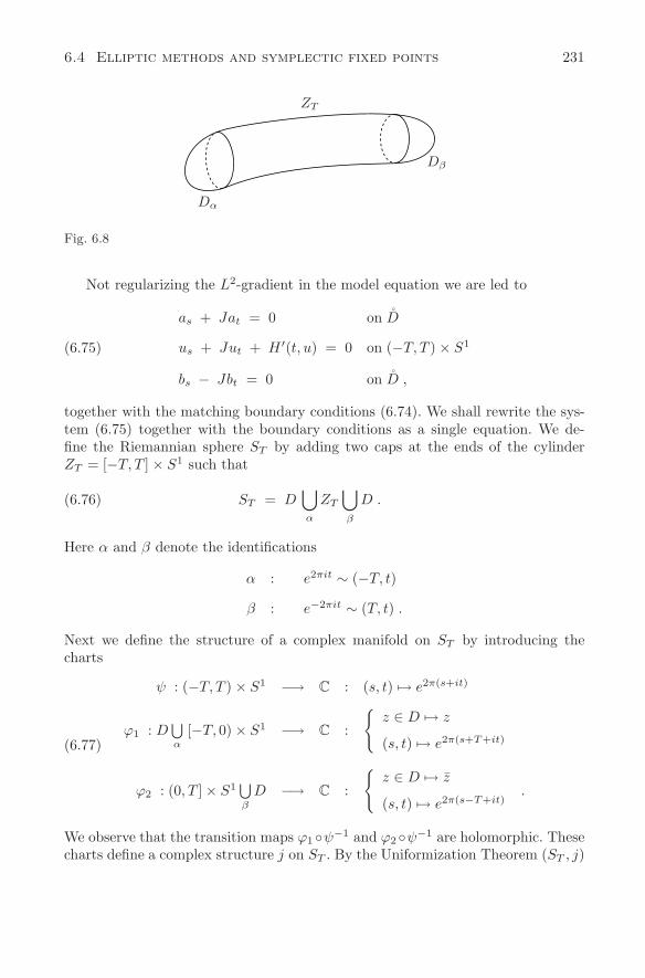
6.4 Elliptic methods and symplectic fixed points 231
Dα
ZT
Dβ
Fig. 6.8
Not regularizing the L2-gradient in the model equation we are led to
as + Jat = 0 on D
us + Jut + H ′(t, u) = 0 on (−T, T ) × S1
bs − Jbt = 0 on D ,
(6.75)
together with the matching boundary conditions (6.74). We shall rewrite the sys-tem (6.75) together with the boundary conditions as a single equation. We de-fine the Riemannian sphere ST by adding two caps at the ends of the cylinderZT = [−T, T ] × S1 such that
ST = D⋃α
ZT
⋃β
D .(6.76)
Here α and β denote the identifications
α : e2πit ∼ (−T, t)
β : e−2πit ∼ (T, t) .
Next we define the structure of a complex manifold on ST by introducing thecharts
ψ : (−T, T ) × S1 −→ C : (s, t) → e2π(s+it)
ϕ1 : D⋃α
[−T, 0) × S1 −→ C :
z ∈ D → z
(s, t) → e2π(s+T+it)
ϕ2 : (0, T ] × S1⋃β
D −→ C :
z ∈ D → z
(s, t) → e2π(s−T+it).
(6.77)
We observe that the transition maps ϕ1ψ−1 and ϕ2ψ−1 are holomorphic. Thesecharts define a complex structure j on ST . By the Uniformization Theorem (ST , j)
232 Chapter 6 The Arnold conjecture, Floer homology . . .
is bi-holomorphic to (S2, i), where S2 = C ∪ ∞ is the standard Riemanniansphere, see, e.g., O. Forster [92]. For notational convenience we denote the α-discby D1 and the β-disc by D2. Consider now v ∈ C∞(ST , T 2n) and define a mapLv, which is smooth on D1, D2 and (−T, T ) × S1 as
Lv = Tv + J (Tv) j + χ[−T,T ]×S1
(H ′(v)ds − JH ′(v)dt
).(6.78)
Here (s, t) are the coordinates on [−T, T ]×S1 and χ[−T,T ]×S1 is the correspondingcharacteristic function on ST . Moreover Tv is the tangent map of v : ST → T 2n.Observe that (Lv)(z) is a linear map TzST → Tv(z)T
2n, which satisfies the relation
−J (Lv)(z) = (Lv)(z) j .
We denote by AT 2n → ST ×T 2n the vector bundle whose fibre over (z,m) consistsof all complex anti-linear maps γ : TzST → TmT 2n, satisfying γj = −Jγ. If vis a map ST → T 2n, we denote by v∗AT 2n the pullback of AT 2n by the graphz → (z, v(z)) of v. Then Lv may be viewed as a section of v∗AT 2n → ST . Assumev is continuous and smooth on ST \(±T, t)|t ∈ S1 and moreover satisfies Lv = 0away from the circle ±T × S1. That precisely means that Lv is the zero sectionof v∗AT 2n → ST . Consider the vector field ∂
∂son (−T, T ) × S1. Then
0 = (Lv)(s, t)( ∂∂s)
= vs + Jvt + H ′(t, v) .
We see that v satisfies differential equation (6.75) on (−T, T ) × S1. On D1 andD2 we have vs + Jvt = 0 and vs − Jvt = 0 respectively. Moreover, the boundaryconditions are satisfied on the common parts of D1, D2 and [−T, T ] × S1.
This new construction can easily be generalized to arbitrary compact symplec-tic manifolds. For this let us denote by j the complex structure on ST and by Jan almost complex structure compatible with ω on M . For v : ST → M we definethe section Lv of v∗AM by
(Lv)(z) = Tv(z) + J(v) Tv(z) j
+χ[−T,T ]×S1(z)[H ′
(t, v(z)
)ds − J
(v(z)
)H ′
(t, v(z)
)dt
].
(6.79)
In order to study the equation Lv = 0, we need to develop a suitable functionalanalytic set up. If 2 < p < ∞ we consider the Banach manifold W 1,p(ST ,M)consisting of maps from ST into M belonging to the Sobolev class W 1,p. For theconstruction of a natural differentiable structure on W 1,p(ST ,M) we refer thereader to the article by H. Eliasson [79]. For v ∈ W 1,p(ST ,M) we consider thebundle v∗AM → ST and let Lp(v∗AM ) be the associated space of Lp-sections.Then, we can equip
Lp(W 1,p(ST ,M)∗AM
)=
⋃v∈W1,p(ST ,M)
v × Lp(v∗AM )
6.4 Elliptic methods and symplectic fixed points 233
with the structure of a Banach space bundle over the Banach manifoldW 1,p(ST ,M). Summing up we have formulated the elliptic system (6.75) to-gether with the matching boundary conditions (6.74) in such a way that solu-tions are to be found as the zeroes of the section L of the Banach space bundleLp(W 1,p(ST ,M)∗AM ) → W 1,p(ST ,M). We shall denote the set of solutions byXT = v ∈ W 1,p(ST ,M)|L(v) = 0.
Note that we cannot expect a solution v : ST → M of L(v) = 0 to be ofregularity better than W 1,p near the boundary ∂ZT of the cylinder ZT . This isdue to the non-smoothness of the cut-off function s → χ[−T,T ](s) at the boundarycomponents s = ±T of ZT . Recall that these two boundary components agreewith the boundaries of the two disks D glued to the cylinder. However, it followsfrom the results in Appendix 5, that a solution v of L(v) = 0 is smooth except at∂ZT where the derivatives in s (i.e., normal to the boundaries) do not match. Tobe more precise we have W 1,p(ST ,M) ⊂ C0(ST ,M) by the Sobolev embeddingtheorem, since p > 2. Hence v being continuous can be studied in local coordinates.If z is a point in the interior of the cylinder ZT we have, in local coordinates,v ∈ W 1,p(Bε, R
2n) with a small open ball Bε centered at z. Moreover v is a weaksolution of a special system of first order elliptic equations and we conclude thatv ∈ C∞(Bε, R
2n) by the “inner” regularity theory of elliptic partial differentialequations. Similarly, the solution v of L(v) is smooth in the interior of the disksD. It is proved in Appendix 5 that, in addition, v has smooth extensions from theinterior of ZT to its boundary ∂ZT and also from the interior of the disks to theirboundaries ∂D1 ∪ ∂D2 = ∂ZT . This does, of course, not mean that the solutionsfit smoothly at the boundary, since the derivatives (in s) normal to the boundarydo not agree. But the restriction of v to the boundary ∂ZT is smooth, so that, inparticular, v(−T ) and v(T ) are smooth loops belonging to C∞
c (S1,M).
We can now use the variational structure of our problem to derive a naturala priori estimate for solutions v ∈ XT . Recall the assumption ω|π2(M) = 0 andassume that L(v) = 0. Let C > 0 be a constant bounding |max
(t,x)H(t, x)| and
|min(t,x)
H(t, x)|. We estimate
ΦH
(v(−T )
)=
∫D1
v∗ω −1∫0
H(t, v(−T, t)
)dt
≥ − max(t,x)
H(t, x) ≥ − C .
We have used that for holomorphic maps
∫
D1
v∗ω =12
∫
D1
|∇v|2J ds dt ≥ 0 .
234 Chapter 6 The Arnold conjecture, Floer homology . . .
Similarly
ΦH
(v(T )
)=
∫D2
v∗ω −1∫0
H(t, v(T, t)
)dt
≤ −min(t,x)
H(t, x) ≤ C ,
using that for anti-holomorphic maps∫
D2
v∗ω = −12
∫
D2
|∇v|2J ≤ 0 .
Summarizing, we have proved
Lemma 3. There exists a constant C > 0, independent of T > 0 such that everysolution v : ST → M of Lv = 0 satisfies
−C ≤ ΦH
(v(−T )
)≤ ΦH
(v(s)
)≤ ΦH
(v(T )
)≤ C , for − T ≤ s ≤ T .
From this we conclude
Lemma 4. There exists a constant C > 0, independent of T > 0 such that everysolution v ∈ W 1,p(ST ,M) of Lv = 0 satisfies
12
T∫
−T
1∫
0
[∣∣∣∂v
∂s
∣∣∣2J
+∣∣∣∂v
∂t− XHt
(v)∣∣∣2J
]ds dt ≤ 2C .
Proof. We compute, using Lemma 3,
2C ≥ ΦH
(v(T )
)− ΦH
(v(−T )
)
=T∫
−T
dds ΦH
(v(s)
)ds =
T∫−T
||Φ′H
(v(s)
)||2J,L2 ds
= 12
T∫−T
[|| d
ds v(s)||2J,L2 + ||v(s) − XHt
(v(s)
)||2J,L2
]ds
= 12
T∫−T
1∫0
[|∂v∂s
(s, t)|2J + |∂v∂t
− XHt
(v(s, t)
)|2J
]ds dt .
Here || ||J,L2 is the L2-norm for sections associated to the Riemannian metric gJ . Our next aim is to study compactness properties of the space X∞ of “bounded
orbits” defined by
X∞ =u ∈ C∞(R × S1,M)
∣∣∣ us + J(u)ut + H ′(t, u) = 0,
u(s) ∈ C∞c (S1,M)and
(ΦH(u(s)
)s∈R
is bounded in R
.
(6.80)
6.4 Elliptic methods and symplectic fixed points 235
We note that for the estimates it is convenient in the following to view M as acompact submanifold of some R
N via Whitney’s embedding theorem, see, e.g., M.Hirsch [113]. Since C∞(R × S1, RN ) is a Frechet space with the usual translationinvariant metric d we may view C∞(R × S1,M) as a closed subspace of C∞(R ×S1, RN ). The induced metric we denote also by d. We shall see that X∞ is acompact subspace of C∞(R × S1, RN ). We begin with
Proposition 10. There exists a constant C > 0 such that for every u ∈ X∞ we have
ΦH
(u(s)
)∈ [−C,C] , s ∈ R .
Proof. By assumption ΦH(u(R)) is bounded in R. Hence, abbreviating || || =|| ||J,L2 ,
+∞∫
−∞
||Φ′H
(u(s)
)||2 ds =
+∞∫
−∞
( d
dsΦH(u(s))
)ds < +∞ .
Consequently there exists a sequence (sn) ⊂ R, with sn → +∞, such that
ΦH
(u(sn)
)−→ α ∈ R and ||Φ′
H
(u(sn)
)|| −→ 0 .
Defining xn = u(sn) ∈ C∞(S1,M) we obtain
||xn − XH(xn)|| −→ 0 .(6.81)
Considering xn as a map into RN we deduce by the compactness of M that
||xn||L2(S1,RN ) ≤ const, where we used the usual L2-inner product. Hence wefind a subsequence satisfying
xn x weakly in H1,2(S1, RN )
xn → x strongly in C0(S1, RN ) .(6.82)
The latter convergence follows using the Arzela-Ascoli Theorem. From (6.81) and(6.82) we conclude that xn is a Cauchy-sequence in L2 so that
xn → x in H1,2(S1,M) and x = XH(x) .(6.83)
Consequently x ∈ C∞(S1,M) and x is a 1-periodic solution of the Hamiltonianvector field. Now ΦH(xn) → ΦH(x) and hence α = ΦH(x). We can argue similarlyfor sequences xn = u(sn) where sn → −∞. By the Arzela-Ascoli Theorem the setof all 1-periodic solutions x = XH(x) is compact in C∞(S1, RN ), so that the setof critical levels
C : =
ΦH(x) |Φ′H(x) = 0
is compact in R. We choose C > 0 so large that the interval [−C,C] contains C.Since s → ΦH(u(s)) is monotone and since, as we have seen, the bounded solutionu connects critical points we conclude that −C ≤ ΦH (u(s)) ≤ C for all s ∈ R
completing the proof of the proposition.
236 Chapter 6 The Arnold conjecture, Floer homology . . .
Corollary 1. X∞ is closed in C∞(R × S1,M).
Proof. Pick any sequence (un) ⊂ X∞. We know from Proposition 10 thatΦH(un(R)) ⊂ [−C,C]. Assume un → u for the C∞-metric d. We obtain for everyr > 0
C ≥ ΦH
(un(r)
)≥ ΦH
(un(−r)
)≥ −C .
Hence, as n → ∞ the estimate implies that ΦH(u(R)) ⊂ R is bounded. Moreover,since ∂un
∂s+ J(un)∂un
∂t+ H ′(t, un) = 0, we may pass to the limit and see that
u satisfies the differential equation as well. This shows that indeed u ∈ X∞ asclaimed.
The geometric picture is as in Section 6.2: a “bounded orbit” u ∈ X∞ connects1-periodic solutions of the Hamiltonian equation x = XH(x) on M . We nextprove that X∞ is a compact subset of C∞(R × S1,M). Note that the metricspace C∞(R × S1,M) has the Heine-Borel property; this is a consequence of theArzela-Ascoli Theorem applied to all the derivatives of the functions. Since, bythe Corollary, X∞ is a closed set we have to show that X∞ ⊂ C∞(R × S1,M)is bounded. This requires that for every compact K ⊂ R × S1 and every integern ∈ N there is a constant CK,n > 0, such that
sup |Dαu(s, t)| ≤ CK,n for all u ∈ X∞ .(s, t) ∈ K|α| ≤ n
(6.84)
The important ingredient for the proof of (6.84) is a gradient estimate uniform inu ∈ X∞. Here we shall use the assumption ω|π2(M) = 0 in a crucial way. Notethat in order to work in local coordinates we have to make sure that, for a wholesequence of mappings, a fixed local neighborhood of a point is mapped into thesame chart of the image space.
Theorem 8. Suppose ω|π2(M) = 0. Then there exists a constant A > 0 such that
|∇u(s, t)|J ≤ A
for all u ∈ X∞ and (s, t) ∈ R × S1.
Proof. Arguing indirectly we find sequences (sk, tk) ∈ R×S1 and (uk) ⊂ X∞ suchthat
|∇uk(sk, tk)|J −→ +∞ .
Since X∞ is invariant under the R-action (6.64) we may assume that sk = 0replacing uk by uk · sk. Moreover, taking a subsequence we may assume tk → t0.Pick any sequence (εk) satisfying
εk > 0 , εk → 0 , εk|(∇uk)(sk, tk)|J −→ +∞ .(6.85)
We wish this sequence to meet additional conditions and use a little trick. It isbased on the following:
6.4 Elliptic methods and symplectic fixed points 237
Lemma 5. Let (X, d) be a complete metric space and g : X → [0,+∞) a continuousmap. Assume x0 ∈ X and ε0 > 0 are given. Then there exists x ∈ X and ε > 0such that
0 < ε ≤ ε0
g(x)ε ≥ g(x0)ε0
d(x, x0) ≤ 2ε0
g(y) ≤ 2g(x) for all y satisfying d(y, x) ≤ ε .
Proof of Lemma 5. Assume there is no x1 ∈ X satisfying d(x1, x0) ≤ ε0 andg(x1) > 2g(x0). Then the statement follows taking x = x0 and ε = ε0. Otherwisewe can pick such an x1 and, proceeding inductively, we can assume there arex0, x1, . . . , xn satisfying
d(xk, xk−1) ≤ ε0
2k−1and g(xk) > 2g(xk−1)
for all 1 ≤ k ≤ n. Then if there does not exist an xn+1 with
d(xn+1, xn) ≤ ε0
2nand g(xn+1) > 2g(xn),(6.86)
the statement follows choosing x = xn and ε = ε02n . Indeed xn satisfies d(xn, x0) ≤
d(xn, xn−1) + · · ·+ d(x1, x0) ≤ 2ε0, and g(xn) > 2g(xn−1) > 22g(xn−2) > 2ng(x0)and hence g(xn)ε > g(x0)ε0. Moreover, from (6.86) we conclude that if d(y, xn) ≤ε, then g(yn) ≤ 2g(xn), hence proving the claim. If, on the other hand, thereexists an xn+1 satisfying (6.86) we continue the process. It must terminate afterfinitely many steps since otherwise we have a Cauchy sequence (xn) ⊂ X satisfyingg(xn) → +∞. This is not possible, since xn → x∗ and g is continuous at x∗.
In order to simplify the notation we shall write in the following | · | instead ofthe Riemannian norm | · |J on the tangent space. In view of the above lemma wecan replace xk = (sk, tk) and εk by slightly modified sequences and may assume,again using the R-action, that the above sequence uk satisfies, in addition
|∇uk(s, t)| ≤ 2|∇uk(0, tk)| , if |s|2 + |t − tk|2 ≤ ε2k, 0 ≤ tk ≤ 1 .(6.87)
Here we conveniently view the maps u as maps defined on R × R by a 1-periodiccontinuation in the t-variable. Rescaling we define a new sequence vk ∈ C∞(R2,M)by
vk(s, t) = uk
((0, tk) +
1Rk
(s, t))
, where Rk = |∇uk(0, tk)| .(6.88)
238 Chapter 6 The Arnold conjecture, Floer homology . . .
Denote by Dk the “large” discs Dk = x = (s, t) ∈ R2| |x| ≤ εkRk ⊂ R
2. Thenthe sequence vk has the following properties:
vk ∈ C∞(Dk,M)
|∇vk(x)| ≤ 2 for x ∈ Dk
|∇vk(0)| = 1
εkRk −→ +∞ .
(6.89)
Moreover vk satisfies the partial differential equation
∂
∂svk + J(vk)
∂
∂tvk = − 1
RkH ′(tk +
t
Rk, vk)(6.90)
on Dk. Since uk ∈ X∞ we find in view of Lemma 4∫
Dk
|∇vk|2 ds dt ≤ 13C ,(6.91)
for k large, with the universal constant C > 0 of Lemma 4. Indeed, introducingthe “small” discs Bk = Bεk
(0, tk) ⊂ R2 we find
∫Dk
|∇vk|2 ds dt =∫
Bk
|∇uk |2 ds dt
=∫
Bk
∣∣∣∂uk
∂s
∣∣∣2 +∣∣∣∂uk
∂t− XH(uk) + XH(uk)
∣∣∣2
ds dt
≤ 3∫
Bk
∣∣∣∂uk
∂s
∣∣∣2 ds dt + 2∫
Bk
∣∣∣XH(uk)∣∣∣2 dsdt
≤ 3∫
R×S1
∣∣∣∂uk
∂s
∣∣∣2 ds dt + lk ≤ 12C + lk ,
where lk → 0 as k → ∞. This proves the claim (6.91). Since the gradients of vk
are uniformly bounded, we shall conclude later on by the elliptic estimates for theequations (6.90) the following crucial:
Lemma 6. Assume the sequence vk satisfies (6.89) and (6.90). Then there existsv ∈ C∞(R2,M) and a subsequence such that
vk → v in C∞ (R2,M) .
Postponing the proof of this lemma, we show next how Theorem 8 follows fromour topological assumption that [ω]|π2(M) = 0. We observe that the smooth mapv guaranteed by the lemma is a holomorphic map of finite and positive area, hencenot a constant map. Indeed from (6.89), (6.90) and (6.91) we deduce the following
6.4 Elliptic methods and symplectic fixed points 239
properties of v:|∇v(0)| = 1
|∇v(x)| ≤ 2 , x ∈ R2
vs + J(v)vt = 0
0 <∣∣∣ ∫R2
v∗ω∣∣∣ = 1
2
∫R2
∣∣∣∇v∣∣∣2 < ∞ .
(6.92)
Define the monotone function Φ(R) for R > 0 by
Φ(R) : = |∫
DR
v∗ω| =12
∫
DR
|∇v|2 12
∫
R2
|∇v|2 .(6.93)
The restriction to the boundary of the holomorphic disc v|DR : DR → M definesthe contractible loop xR : S1 → M by xR(τ) = v(Re2πiτ ). In view of the differen-tial equation in (6.92) this loop satisfies |xR(τ)| = 2πR|∂v
∂s (Re2πiτ )|. Computingin polar coordinates we find that
∫
R2
|∂v
∂s|2 =
∞∫
0
12πR
1∫
0
|xR(τ)|2 dτ dR ,
which is finite in view of (6.92). Consequently, there is a sequence of holomorphicdiscs v|DRj
such that the arc lengths l(xRj) of their boundaries tend to zero as
j → ∞. In order to estimate the area of these discs by the arc length, we coverthe compact manifold M by finitely many open sets Uj ⊂ M , 1 ≤ j ≤ N suchthat each Uj is diffeomorphic to a closed ball. There is a constant d > 0 such thatevery loop x on M having diameter ≤ d is contained in one of the sets Uj . ByPoincare’s lemma we conclude that ω|Uj = dλj for a 1-form λj on Uj . Thereforewe can estimate the action of a loop x(t) ⊂ Uj for t ∈ [0, 1] by the arc length l(x),
|∫
[0,1]
x∗λj | ≤ l(x) ||λj || ,(6.94)
where ||λJ || = max||λJ (m)||,m ∈ Uj, with the standard norm of the linear mapλj(m) ∈ (TmM)∗. Consequently, if γ = max ||λj ||, 1 ≤ j ≤ N , we conclude forevery loop x on M having diameter ≤ d that
|∫
x
λj | ≤ l(x) · γ .(6.95)
Consider now the small loop xR(τ) which is the boundary of the holomorphic discvR. Then it is contained in one of the open sets, say Uj . Since it is contractible we
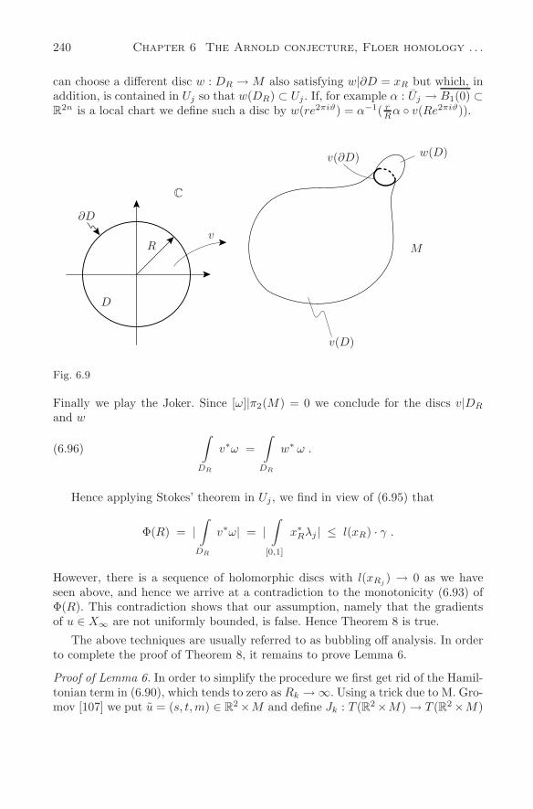
240 Chapter 6 The Arnold conjecture, Floer homology . . .
can choose a different disc w : DR → M also satisfying w|∂D = xR but which, inaddition, is contained in Uj so that w(DR) ⊂ Uj . If, for example α : Uj → B1(0) ⊂R
2n is a local chart we define such a disc by w(re2πiϑ) = α−1( rRα v(Re2πiϑ)).
∂D
D
vR
v(∂D) w(D)
M
v(D)
C
Fig. 6.9
Finally we play the Joker. Since [ω]|π2(M) = 0 we conclude for the discs v|DR
and w∫
DR
v∗ω =∫
DR
w∗ ω .(6.96)
Hence applying Stokes’ theorem in Uj , we find in view of (6.95) that
Φ(R) = |∫
DR
v∗ω| = |∫
[0,1]
x∗Rλj | ≤ l(xR) · γ .
However, there is a sequence of holomorphic discs with l(xRj) → 0 as we have
seen above, and hence we arrive at a contradiction to the monotonicity (6.93) ofΦ(R). This contradiction shows that our assumption, namely that the gradientsof u ∈ X∞ are not uniformly bounded, is false. Hence Theorem 8 is true.
The above techniques are usually referred to as bubbling off analysis. In orderto complete the proof of Theorem 8, it remains to prove Lemma 6.
Proof of Lemma 6. In order to simplify the procedure we first get rid of the Hamil-tonian term in (6.90), which tends to zero as Rk → ∞. Using a trick due to M. Gro-mov [107] we put u = (s, t,m) ∈ R
2 ×M and define Jk : T (R2 ×M) → T (R2 ×M)
6.4 Elliptic methods and symplectic fixed points 241
by
Jk(u)(α, β, h) =(− β, α, J(m)h + βH ′
k(t,m) + αJ(m)H ′k(t,m)
),(6.97)
where H ′k(t,m) = 1
RkH ′(tk + t
Rk,m). One verifies readily that J2
k = −id. Hence Jk
is a sequence of almost complex structures on R2 × M converging together with
all its derivatives uniformly on R2 × M to the almost complex structure i ⊕ J , if
we identify R2 with C in the usual way. Define the sequence vk ∈ C∞(R2, R2×M)
by
vk(s, t) =(s, t, vk(s, t)
).(6.98)
Then, on Dk = BεkRk(0) ⊂ R
2,
∂∂s
vk + Jk(vk) ∂∂t
vk = 0
|∇vk(s, t)| ≤ 4
|∇vk(0, 0)| ≥ 1
εk Rk → ∞ .
(6.99)
The aim is to find a subsequence such that vk → v in C∞(R2, R2 ×M) for a mapv ∈ C∞(R2, R2 × M). In view of the Arzela-Ascoli Theorem it is sufficient to findC∞
loc-bounds for vk, i.e., for every compact set K we have to find uniform (in k)bounds for vk together with all the derivatives. Choosing p > 2 it is sufficient, inview of Sobolev’s embedding theorem to establish on every compact subset K ⊂ R
2
uniform bounds in W l,p(K) instead of Cl(K) for all l ≥ 1. In order to establishsuch W l,p
loc-bounds, we proceed by induction. By assumption the gradients of vk areuniformly bounded so that the W 1,p
loc -bounds are guaranteed. Arguing indirectlywe shall assume now that there are W l,p
loc-bounds but not W l+1,ploc -bounds, for some
l ≥ 1. Hence possibly taking a subsequence of vk, we find a sequence xk ∈ R2 and
a sequence εk > 0 satisfying εk → 0 such that
xk → x0 and |vk|W l+1,p(Bεk(xk))→ +∞ ,(6.100)
where, viewing M as a subset of RN , we consider vk as a map from R
2 into RN .
Since, by assumption, |∇vk| is uniformly bounded we conclude, by the Arzela-Ascoli theorem, for a subsequence, that
vk(x0) → (x0,m) and vk → v in C0loc .(6.101)
This allows us to localize the problem in a coordinate chart. Around (x0,m) ∈R
2 × M there is a chart given by α : U → R2+2n, satisfying α(x0,m) = 0 and
vk
(Bε0(x0)
)⊂ V ⊂ V ⊂ U ,(6.102)
242 Chapter 6 The Arnold conjecture, Floer homology . . .
for some ε0 > 0 and for a suitable open neighborhood V of (x0,m) and for all ksufficiently large. Hence defining the smooth functions uk := α vk : Bε0(x, 0) →R
2+2n, and replacing Jk by Jk defined by
Jk(y) = Tα(α−1(y)
)· Jk
(α−1(y)
)Tα−1(y) ,(6.103)
y ∈ α(U) ⊂ R2+2n we have, on Bε0(x0),
∂uk
∂s + Jk(uk)∂uk
∂t = 0
uk(x0) → 0
|∇uk(x)| ≤ C
|uk|W l+1,p(Bε0 (xk)) → +∞ .
(6.104)
Moreover, Jk → J∞ in C∞ for some almost complex structure J∞ in R2+2n near
0. We shall denote by J0 the following constant complex structure on R2+2n
J0 := J∞(0) , J20 = −1l .
Now we make use of the following well-known elliptic estimate for the Cauchy-Riemann operator. For every 1 < p < ∞, m and n ≥ 0 there exists a constantC > 0 such that
C|u|m+1,p ≤ |us + J0 ut|m,p ,(6.105)
for every smooth function u : R2 → R
2n+2 having compact support in the unitball. This is the classical estimate for the Cauchy-Riemann operator (if written incomplex notation), J0 being constant. For a proof we refer to the monograph byE. Stein [205], p. 60. In order to apply this estimate, we take a smooth functionβ : R → [0, 1] such that β(s) = 1 for |s| ≤ 1
2 and β(s) = 0 for |s| ≥ 1. For λ > 0 wedefine the function αλ(x) := β(x−x0
λ ). Then αλ(x) = 0 if |x− x0| ≥ λ. To simplifythe formulas we shall use the abbreviating notation
|u|l : = |u|W l,p(Bε0 (x0)) ,
where p > 2 is fixed. Moreover, we shall abbreviate α ≡ αλ. We then concludefrom (6.105) that
C |αuk|l+1 ≤ |(αuk)s + J0(αuk)t|l .
By the Cauchy-Riemann equation, (uk)s = −Jk(uk)(uk)t, and
C |αuk|l+1 ≤ C1(λ)|uk|l + |αtJk(uk)uk|l + |[(J0 − Jk(uk)](αuk)t|l .
Using now the Leibniz rule for differentiation and the inductive assumption, name-ly that |uk|l ≤ Cl, we conclude
C |αuk|l+1 ≤ |J0 − Jk(uk)|L∞(Bλ(x0)) · |αuk|l+1 + C3(λ) .
6.4 Elliptic methods and symplectic fixed points 243
Since uk(x0) → 0, uk → u∞ uniformly on Bε0(x0) and J0 = lim Jk(0), we see,that the factor in front of |αuk|l+1 on the right hand side is smaller than C
2, if λ
is sufficiently small, and if k is sufficiently large. Since α ≡ 1 on Bεk(xk) as soon
as k is sufficiently large, we finally conclude
|uk|W l+1,p(Bεk(xk)) ≤ C4 < ∞ ,
if k is sufficiently large. This obviously contradicts the last statement in (6.104)and hence the proof of Lemma 6 is finished.
With Lemma 6, the proof of Theorem 8 is completed: we have uniform gradientestimates for u ∈ X∞. Therefore, we can apply the same arguments as in Lemma6 and obtain C∞
loc-bounds, uniform for u ∈ X∞. In addition, using the R-action(6.95) on X∞ we can get much more, namely Cl
b bounds on R×S1, with the normsdefined by |u|Cl
b= sup |Dαu(s, t)|, where the supremum is taken over |α| ≤ l and
(s, t) ∈ R × S1. We shall show that
supu∈X∞
|u|Clb(R×S1,RN ) < ∞ ,
for every l ≥ 0, so that X∞ is uniformly bounded in C∞(R × S1,M); here weview M again as a subset of R
N . The easiest way to see this is the following.Since the uniform gradient estimate for X∞ holds on all of R × S1, we can takethe R-action on X∞, given by τ · u(s, t) = u(s + τ, t) and only have to prove theuniform Cl estimates for X∞ on a finite covering of the interval s∗× [0, 1] ⊂ R×S1
by compact sets for some fixed s∗ ∈ R. But this we have just done in the proof ofthe previous lemma and the claim is proved. Since X∞ is closed and bounded inC∞(R × S1,M) we have demonstrated
Proposition 11. The set X∞ of bounded orbits is a compact subset of the metricspace C∞(R × S1,M).
On X∞ there is as we have seen a continuous flow which is gradient-like andwe can estimate the number of rest points by Ljusternik-Schnirelman (Theorem6), provided of course that X∞ = ∅. In order to get an insight into the topologyof this set X∞ of bounded orbits we shall proceed as in Section 6.2 and first provethat the sets XT are close to X∞ if T is large. Recall that the space XT is definedas the set of solutions
XT : = u ∈ W 1,p(ST ,M) |Lu = 0 ,(6.106)
where the nonlinear operator L is defined in (6.79). Recall also that we cannotexpect better regularity properties for these solutions, since L contains the non-smooth term χ[−T,T ]×S1H1. Since p > 2 we have W 1,p(ST ,M) ⊂ C0(ST ,M) inview of the Sobolev embedding theorem. However, we shall restrict now the solu-tions u to the cylinder ZT ⊂ ST . By elliptic regularity theory, these restrictions aresmooth as we have pointed out above: u|ZT
∈ C∞(ZT ,M). Moreover, by Lemma
244 Chapter 6 The Arnold conjecture, Floer homology . . .
4, there exists a constant C > 0 such that for every solutions v ∈ XT , the followingestimate (on ZT ) holds
12
T∫
−T
1∫
0
[|∂v
∂s|2J + |∂v
∂t− XHt
(v)|2J]
ds dt ≤ 2C,(6.107)
where C is independent of T > 0. Copying now the above C∞-estimates word forword we find, for every given multi-index α, a constant Cα > 0 such that for everyT > 2 and for every v ∈ XT , the following estimate holds:
max |Dαv(s, t)| | (s, t) ∈ [−T + 2, T − 2] × [0, 1] ≤ Cα.(6.108)
From this we shall conclude that XT is close to X∞ provided T is large enough.To make this statement more precise we take a smooth function β : R → [0, 1]satisfying β(s) = 1 for s ≤ 1, β′(s) > 0 for 1 < s < 2 and β(s) = 0 for s ≥ 2 anddefine the family of cut off functions βT : R → [0, 1] for T ≥ 5 by
βT (s) = 1 for |s| ≤ T − 3
βT (s) = β(s − T + 3) for s ≥ T − 3
βT (s) = βT (−s) for s ≥ 0 .
Given T0 > 5 we define for T ≥ T0 a map
σT : XT → C∞(R × S1,M)
σT (u)(s, t) = u(sβT (s), t
).
(6.109)
By (6.108), we have uniform C∞-estimates on [−T + 1, T − 1]× [0, 1]. Assume weare given an open neighbourhood U of X∞ in C∞(R × S1,M). This means thatthere exists R > 0, ε > 0 and k ∈ N such that every w ∈ C∞(R×S1,M) for whichthere exists an u ∈ X∞ satisfying
| Dα(u(s, t) − w(s, t)) | < ε, for all (s, t) ∈ [−R,R] × S1, and for all |α| ≤ k ,
belongs to U . We conclude that for T large
σT (XT ) ⊂ U.
Indeed, arguing indirectly we find a sequence Tn → ∞ and a sequence un ∈ XTn
such that vn := σTn(un) ∈ U . However, in view of (6.108) we find that (vn) has
a subsequence converging with all its derivative on bounded subsets of R × S1
to some smooth map v : R × S1 → M . Hence we may assume without loss ofgenerality that (vn) converges to some v ∈ U . We observe that for every R > 0
12
R∫
−R
1∫
0
[|∂v
∂s|2J + |∂v
∂t− XHt
(v)|2J]
ds dt ≤ 2C ,(6.110)
6.4 Elliptic methods and symplectic fixed points 245
in view of (6.107). If R → ∞, we obtain
12
+∞∫
−∞
1∫
0
[|∂v
∂s|2J + |∂v
∂t− XHt
(v)|2J]
ds dt ≤ 2C.
Clearly v satisfies the partial differential equation
∂v
∂s+ J(v)
∂v
∂s+ H ′(t, v) = 0.
This implies that v ∈ X∞ hence contradicting the fact that v ∈ U .Summing up we have shown that for a given open neighbourhood U of X∞ in
C∞(R × S1,M), there exists T0 such that, for T ≥ T0, the set σT (XT ) belongs toU . Consequently, we have the following commutative diagram
τU
XT M
U X∞j
τT
τ∞σT
where the maps τT , τ∞ and τU are the evaluation maps at the point (s, t) = (0, 0).Assume now that τ∗
T is injective in cohomology. Then τ∗U is also injective and
we consider the following diagram for the Alexander-Spanier cohomology:
τ∗∞τ∗
U
H∗(U) H∗(X∞)
H∗(M)
j∗
In view of the continuity property of the Alexander-Spanier cohomology, wecan take the direct limit over all open neighborhoods U of X∞ in C∞(R×S1,M)and conclude that the map τ∗
∞ is injective. We see that the set of bounded solutionscontains the cohomology of the underlying manifold M , in particular cup-length(X∞) ≥ cup-length (M). Applying the Ljusternik-Schnirelman Theorem (Theorem6) to the continuous gradient-like flow on X∞, we conclude the desired statement
Theorem 9. (A. Floer, H. Hofer) Assume (M,ω) is a compact symplectic manifoldsatisfying [ω]|π2(M) = 0. Then every smooth time-periodic Hamiltonian vectorfield x = XH(x) on M possesses at least cup-length (M) + 1 contractible periodicsolutions of period 1.
246 Chapter 6 The Arnold conjecture, Floer homology . . .
In order to complete the proof of Theorem 9, we still have to verify that themap τ∗
T is injective. Proceeding as in Section 6.2, we shall use Fredholm theory inorder to approximate XT by smooth compact manifolds of dimension 2n, whosecohomology can be estimated using degree theory. For the following we choose afixed number T > 5 and consider the operator L = LT as a smooth section of thebundle
Lp(W 1,p(ST ,M)∗AM ) =⋃
v∈W1,p(ST ,M)
v × Lp(v∗AM ).
over W 1,p(ST ,M). We abbreviate this bundle by
E → B .
The idea now is to homotope the given section L to the Cauchy-Riemann typesection ∂
∂s + J ∂∂t by considering the homotopy ρ → Lρ, 0 ≤ ρ ≤ 1, defined by
Lρ(v) = Tv + J(v)(Tv)j + ρχ(s)[H ′(t, v)ds − J(v)H ′(t, v)dt].
Introducing the evaluation map τ : B → M by v → v(0, 0) we define the associatedhomotopy Lρ, 0 ≤ ρ ≤ 1 by
Lρ(v) =(Lρ(v), τ(v)
), 0 ≤ ρ ≤ 1 .
This is, by definition, a map from B into E × M , for every 0 ≤ ρ ≤ 1. We mayview E ×M as a Banach manifold bundle over B. For ρ = 0, the equation L0(v) =(0,m), for given m ∈ M , only has the constant solution v0 ≡ m, since there areno nontrivial holomorphic spheres because of our assumption [ω]|π2(M) = 0 onthe manifold M . The linearization at this particular section v0 gives in the firstcomponent the linear Cauchy-Riemann operator, and in the second componentthe evaluation at 0. To be more precise, denoting by D = L′
0(v0) the linearizationat the particular point v0 ≡ m, one computes that
Dh = (Th + J(m)(Th)j, h(0)).
In view of the results in Appendix 4, the operator D : W 1,p(ST , TmM) →Lp(v∗
0AM ) × TmM is an isomorphism. Now we use the Z2-degree for Fredholmsections having Fredholm index zero. Given the necessary compactness conditionswe have just demonstrated that this degree is equal to 1. Let us assume for the mo-ment that the set of solutions of Lρ(v) = 0, 0 ≤ ρ ≤ 1 is compact. Then there existsan open neighborhood of this solution set on which the Fredholm map is proper,see S. Smale [201]. Consequently, by the homotopy property of the Z2-index, theoriginal map for ρ = 1 given by v → (L1(v), τ(v)) has also Z2-degree equal to 1.To continue our line of thought, let us also assume for the moment that the imageof the map v → L1(v) is transversal to the zero section 0E of the bundle E . Then
6.4 Elliptic methods and symplectic fixed points 247
the preimage of 0E is a smooth compact submanifold Σ of B with dimension 2n.Moreover, the evaluation map τ := τ |Σ : Σ → M , defined by v → v(0, 0) will haveZ2-mapping degree equal to 1. This allows us to argue precisely as in Proposition 5of Section 6.2 in order to prove that in Alexander-Spanier cohomology the map τ∗
T
is injective as desired, hence completing the proof of Theorem 9. To reach this con-clusion, we assumed all the necessary compactness properties and, in addition, thetransversality of the image of v → L1(v) to the zero section 0E . The transversal-ity can be established by an arbitrary C∞-small perturbation of the HamiltonianH. However, the argument is quite intricate and we refer the reader to A. Floer,H. Hofer and D. Salamon [87] for a proof. Hence with this perturbation argumenttogether with the continuity property of the Alexander-Spanier cohomology, weare left with the compactness question, and it remains to prove the following
Proposition 12. Assume 2 < p < ∞ and [ω]|π2(M) = 0. Then the set of solutions
XT : = (ρ, v) ∈ [0, 1] × W 1,p(ST ,M) |Lρ(v) = 0
is compact in [0, 1] × W 1,p(ST ,M).
Proof of Proposition 12. If v ∈ XT we define the number ε(v) ≥ 0 by
ε(v) = infε > 0∣∣∣ there exists z ∈ ST(6.111)
satisfying |∇v|p,Bε(z) = ε2−p
p .
Here Bε(z) denotes the ε-ball around z for some fixed metric on ST . (The choiceof the metric is irrelevant since ST is compact.) Note that the function ε →ε
p−2p |∇v|p,Bε(z) is nondecreasing. Assume now that
infv∈XT
ε(v) ≡ ε > 0 .
Then|∇v|p,Bε(v)(z) ≤ ε
2−pp
for every z ∈ ST , and hence we have a W 1,p-bound for XT . This bound implies thecompactness of XT in [0, 1] × W 1,p(ST ,M) as we shall show next. Viewing M asa subset of some R
N , we can consider W 1,p(ST ,M) as a subset of W 1,p(ST , RN ).Pick a sequence (ρk, vk) ∈ XT ; then we have to find a convergent subsequence.By taking a suitable subsequence we can assume that ρk → ρ, and vk → v inC0(ST , RN ) (in view of the compact embedding of W 1,p(ST , RN ) ⊂ C0(ST , RN ))and vk v weakly in W 1,p(ST , RN ) for some v ∈ W 1,p(ST , RN ) (in view ofthe reflexivity of the space W 1,p(ST , RN )). We shall show that vk is a Cauchysequence in W 1,p(ST , RN ). Since we have convergence in C0(ST , RN ) we now canwork locally in charts of ST and of M as well. Any difficulty that may arise occursnear the boundary ∂ZT ⊂ ST of cylinder ZT ⊂ ST , since away from this boundary,
248 Chapter 6 The Arnold conjecture, Floer homology . . .
the maps u ∈ XT are smooth (by elliptic regularity theory) and we can thereforeestablish C∞-bounds arguing as above. Hence we carry out the local argumentfor the worst case only focussing on the lower cap of ST . In order to find localcoordinates on ST near the boundary ∂ZT belonging to the lower cap we take abiholomorphic embedding ϕ of [−1, 1]×S1 into ST satisfying ϕ(s, t) = (s−T, t) forall 0 ≤ s ≤ 1. Choosing now symplectic coordinates on M we are confronted withthe following situation. We have a sequence of mappings vk ∈ W 1,p(Bε(0), R2n)and a sequence of numbers ρk ∈ [0, 1] satisfying
vk −→ v in C0(Bε(0), R2n
)
vk v in W 1,p(Bε(0), R2n
)
ρk −→ ρ ,
where v ∈ W 1,p(Bε(0), R2n) and v(0) = 0, and where Bε(0) ⊂ R2 is the open disk
centered at (s, t) = (0, 0). Moreover, these maps satisfy the following system offirst order elliptic partial differential equations
∂vk
∂s+ J(vk)
∂vk
∂t+ ρkχ(s)H ′(t, vk) = 0
on Bε(0), where χ is the characteristic function of the positive half line in s. Weconclude that v solves the equation
∂v
∂s+ J(v)
∂v
∂t+ ρχ(s)H ′(t, v) = 0 .
We shall prove that vk is a Cauchy sequence in W 1,p(Bρ(0), R2n) for some smallρ > 0. Let β : R
2 → [0, 1] be a smooth function having its support in the unit diskand taking on the value 1 on the smaller disk of radius 1/2. For τ > 0 we thendefine the function βτ on R
2 by βτ (z) = β(z/τ). By J0 we denote the constantalmost complex structure J(0) on R
2n. Finally, we write |.|j for the W j,p-normon the ε-disk in R
2, recalling that 2 < p < ∞ and fixed. If 0 < τ < ε we nowcompute, using the classical estimate (6.105) for the Cauchy-Riemann operator,
c|βτ (vk − v)|1 ≤ |∂(βτ (vk − v))|0
≤ | ∂
∂s(βτ (vk − v)) + J(v)
∂
∂t(βτ (vk − v))|0
+|J0 − J(v)|L∞(Bτ )|βτ (vk − v)|1
≤ |βτ (∂
∂s(vk − v) + J(v)
∂
∂t(vk − v))|0 + c1(τ)|vk − v|0
+σ(τ)|βτ (vk − v)|1.
6.4 Elliptic methods and symplectic fixed points 249
Here σ(τ) → 0 for τ → 0, and c1(τ) is a constant depending on τ . Hence, if τ > 0is small enough,
c
2|βτ (vk − v)|1 ≤ c1(τ)|vk − v|0 + |J(v) − J(vk)|L∞(Bτ )|vk|1
+|ρkχH ′(t, vk) − ρχH ′(t, v)|0 .
By assumption, |vk|1 is a bounded sequence, |vk − v|0 → 0, J(vk) → J(v) uni-formly on Bε(0) and |ρkH ′(t, vk) − ρχH ′(t, v)|0 → 0. Consequently vk → v inW 1,p(Bδ(0), R2n) for some δ > 0 sufficiently small. Covering ST by finitely manycharts we have demonstrated the vk → v in W 1,p(ST ,M), so that XT is compact,as claimed in the proposition.
To finish our argument, it remains to verify our assumption that the numbersε(v) are uniformly bounded away from 0 on the set XT . We argue by contradiction,assuming that we have no uniform W 1,p-bound on XT , that we find a sequence(ρk, vk) ∈ XT satisfying ε(vk) → 0. By the definition of ε(v) we find a sequencezk ∈ ST such that with εk := ε(vk) we have
|∇vk|0,Bεk(z) ≤ |∇vk|0,Bεk
(zk)
for all z ∈ ST . Moreover,
1 = εp−2
p
k |∇vk|0,Bεk(zk) .
Since εk → 0, and since we have C∞ bounds away from ∂ZT , we deduce that dist(zk, ∂ZT ) → 0. Hence, after taking a subsequence, we can assume that zk → z0 ∈∂ZT . The argument now is similar to the one used previously in the bubbling offanalysis. Namely we rescale near zk and obtain in this way a new sequence for whichwe have a W 1,p
loc -bound. Therefore, arguing as above, the new sequence, uk, will beW 1,p
loc -precompact. Hence taking a convenient subsequence we can pass to the limitand obtain a solution v ∈ W 1,p(C,M) of vs + J(v)vt = 0 on C, which is nonzero.By ellitpic regularity theory v ∈ C∞(C,M). Moreover,
∫R|∇v|2Jdsdt < ∞; this
follows from (6.110) applied to our sequence uk, together with the following apriori estimate for the caps:
|∫
D
u∗k ω| ≤ 2C ,
which follows immediately from the estimate before Lemma 3. Arguing now as inthe proof of Theorem 8, we arrive at a contradiction to our topological assumption[ω]|π2(M) = 0. The proof of Proposition 12, and therefore the proof of Theorem9 is complete.
250 Chapter 6 The Arnold conjecture, Floer homology . . .
Remarks: We note that the torus (T 2n, ω) meets the assumption of Theorem 9 forevery symplectic structure ω.
Theorem 9 is due to A. Floer [86] and H. Hofer [115], 1987. They both derive theresult from a more general intersection result for compact Lagrangian manifolds.M. Chaperon, in his Bourbaki lecture [42] 1982–83, had already noticed that thevariational approach is applicable to the global intersection problem of Lagrangianmanifolds suggested by V.I. Arnold in [9].
The cohomology in the above statement uses Z2 coefficients and we wouldlike to point out that the statement actually holds for every coefficient field. Theproof, however, requires more intricate tools from Fredholm theory and algebraictopology. The crucial point is to resolve a number of orientation questions for adistinguished class of Fredholm operators. For the technology involved, we refer toA. Floer and H. Hofer [89]. It turns out that XT has a natural orientation inheritedfrom the orientation of (M,ω) provided it is a manifold.
The above proof of the Arnold conjecture for a general symplectic manifold(M,ω) crucially uses the restrictive assumption requiring [ω]|π2(M) = 0, andwe point out that without this assumption the conjecture is still open. However,more can be said if one (a priori) requires that all the 1-periodic solutions of theHamiltonian vector field under consideration are nondegenerate, as we shall see inthe next section.
6.5 Floer’s approach to Morse theory for the action functional
We shall sketch Floer’s seminal approach to solving the Arnold conjecture in thenondegenerate case where one assumes that all the 1-periodic solutions of theHamiltonian system on (M,ω) are nondegenerate. Since M is compact, there areonly finitely many such 1-periodic solutions. Floer studies the set of bounded or-bits of the unregularized gradient equation defined by the action functional on thespace of contractible loops of M . The bounded orbits are special solutions of a dis-tinguished system of first order elliptic equations of Cauchy-Riemann type, as wehave shown above. But unlike the general case studied in the previous section, inthe nondegenerate case the bounded orbits tend in a strong sense asymptoticallyto the 1-periodic solutions of the Hamiltonian equation. This additional structureof the solution set is used by Floer in order to construct by means of Fredholmtheory a chain complex generated by the finitely many 1-periodic solutions. Thehomology of this complex is called Floer homology; it is an invariant of the under-lying manifold. By continuing the complex to the classical Morse complex definedby the gradient system y = −∇H(y) of the Hamiltonian function on M , Floer fi-nally shows that his homology is a model of the singular homology of the manifold.This then finishes the proof of the Arnold conjecture.
6.5 Floer’s appraoch to Morse theory . . . 251
We consider a compact symplectic manifold (M,ω) of dimension 2n restrictedby the requirement that [ω]|π2(M) = 0. This means that the integral of the sym-plectic structure vanishes over every sphere
∫
S2
u∗ω = 0 , u : S2 → M .(6.112)
To the smooth time-dependent Hamiltonian function H : S1 × M → R, periodicin time, H(t, x) = H(t + 1, x) for t ∈ R and x ∈ M we associate as usual theHamiltonian vector field XH : R × M → TM by ω(XH , ·) = −dxH(t, x). Thesolutions x(t) of the time-dependent Hamiltonian equation
x(t) = XH
(t, x(t)
)on M(6.113)
define the flow ψt by ψt(x(0)) = x(t). We are looking for periodic solutions x(t +1) = x(t) which are contractible loops on M , x 0. We shall assume that all thecontractible periodic solutions x(t) are nondegenerate, requiring for the flow mapψ = ψ1 that
det(1 − dψ(x(0))
)= 0 .(6.114)
By PH we shall denote the set of these periodic solutions:
PH = x : S1 → M | x(t + 1) = x(t), x solves (6.113) and (6.114),
and x 0 .(6.115)
Note that this is a finite set, since M is compact and the nondegenerate 1-periodicsolutions are isolated in M . By Ω we shall denote the set of smooth contractibleloops γ of M , where, as usual, S1 = R/Z. A loop is represented by its coverγ : R → M satisfying γ(t + 1) = γ(t). The required 1-periodic solutions aredistinguished in Ω as the critical points of the action functional ϕH : Ω → R
defined by
ϕH(γ) = −∫
D
γ∗ω +
1∫
0
H(t, γ(t)
)dt .(6.116)
Here D ⊂ C denotes the closed unit disc and γ : D → M is a smooth functionextending γ and hence satisfying γ(e2πit) = γ(t). Such an extension exists since γis assumed to be contractible and it follows from the assumption (6.112) that thefirst integral on the right hand side of (6.116) does not depend on the choice ofthe extension and hence depends only on the loop γ. With TγΩ we shall denote
252 Chapter 6 The Arnold conjecture, Floer homology . . .
the tangent space at γ ∈ Ω consisting of the smooth vector fields ξ ∈ C∞(γ∗TM)along γ satisfying ξ(t + 1) = ξ(t). Computing the derivative of ϕH at γ in thedirection of ξ, one finds readily that
dϕH(γ)ξ =
1∫
0
ω(γ, ξ) + dH(t, γ)ξ dt ,(6.117)
which indeed vanishes for every ξ ∈ TγΩ if and only if the loop γ ∈ Ω is a solutionof the Hamiltonian equation (6.113). It is convenient to choose an almost complexstructure J on M compatible with ω (see Chapter 1). This is an endomorphismJ ∈ C∞ (End TM), i.e., Jx ∈ L(TxM,TxM) satisfying J2 = −1 such that
g(ξ, η) = ω(ξ, J(x)η
), ξ, η ∈ TxM(6.118)
defines a Riemannian metric g on M . The Hamiltonian vector field is then repre-sented by
XH(t, x) = J(x)∇H(t, x) ,(6.119)
where ∇ denotes the gradient of a function on M with respect to the x-variablein the metric g above. For the derivative we obtain
dϕH(γ)ξ =
1∫
0
g(J(γ)γ + ∇H(t, γ), ξ
)dt ,(6.120)
so that the gradient of ϕH with respect to an induced L2 metric on Ω is given by
grad ϕH(γ) = J(γ)γ + ∇H(γ) ∈ TγΩ .(6.121)
However, the gradient equation
d
dsx = − grad ϕH(x) , x ∈ Ω(6.122)
does not determine a flow. As we have pointed out in the previous section, due toa loss of derivatives there is no Banach space setup in which grad ϕH(x) can beconsidered as a vector field on a Banach manifold. Indeed the initial value problemdefined by (6.122) on Ω is not well-posed. Floer views a solution x of (6.122) as amap
u : R × S1 −→ M , (s, t) → u(s, t) = u(s, t + 1)(6.123)
which solves the partial differential equation
∂u
∂s+ J(u)
∂u
∂t+ ∇H(t, u) = 0 .(6.124)
6.5 Floer’s appraoch to Morse theory . . . 253
The crucial objects from now on, are therefore the solutions u : R × S1 → M ofthe nonlinear partial differential equation (6.124), which are contractible so thatu(s, ·) ∈ Ω. These solutions correspond to the flow lines of the gradient equation(6.122). The equation (6.124) is a perturbation of a Cauchy-Riemann equation. Asmooth map u : S2 → M solving the Cauchy-Riemann equation
∂u
∂s+ J(u)
∂u
∂t= 0(6.125)
is called a holomorphic sphere. It satisfies∫
S2
u∗ω =12
∫
S2
|∇u|2 ,(6.126)
so that our assumption (6.112) excludes, in particular, nonconstant holomorphicspheres.
From the torus case we know that not all solutions of (6.124) are relevantand we are interested only in the set of “bounded orbits” which we denote byM ≡ M(H, J). This set is defined as the set of smooth mappings u : R×S1 → Mwhich are contractible, solve the equation (6.124) and have, in addition, finite“energy”
E(u) : =12
∞∫
−∞
1∫
0
∣∣∣∂u
∂s
∣∣∣2 +∣∣∣∂u
∂t− XH(t, u)
∣∣∣2
ds dt < ∞ .(6.127)
Equivalently M is the space of contractible solutions u along which the decreasingfunction ϕHu(s) remains bounded for all s ∈ R, where u(s)(t) = u(s, t) ∈ Ω.
Floer proves in [85] that the space M of bounded solutions of the partialdifferential equation (6.124) has a structure which looks like that of a Morse-Smale system on a smooth, compact, and finite dimensional manifold, as we nowdescribe.
Since M is compact and since [ω] vanishes over π2(M) according to the as-sumption (6.112) it follows using elliptic regularity theory that the set of solutionsM is compact in the topology of uniform convergence with all derivatives on com-pact sets. This is not easy to prove and we refer to A. Floer [85], D. Salamon [188],and H. Hofer and D. Salamon [119]. Moreover, for every bounded orbit u ∈ Mthere exists a pair x, y ∈ PH of periodic solutions, such that u is a connectingorbit from y to x, i.e.,
lims→−∞
u(s, t) = y(t) , lims→+∞
u(s, t) = x(t) ,(6.128)
the convergence being uniformly in t as |s| → ∞ and ∂u∂s
converging to zero againuniformly in t. Given two periodic solutions x, y ∈ PH we abbreviate by
M(y, x) = M(y, x;H, J)(6.129)
254 Chapter 6 The Arnold conjecture, Floer homology . . .
the set of solutions u ∈ M satisfying the asymptotic boundary conditions (6.128).For the energy one computes
E(u) = ϕH(y) − ϕH(x) , if u ∈ M(y, x) .(6.130)
The energy is positive for nonconstant orbits. From the previous section we knowthat the set M of solutions consists of the periodic solutions and the connectingorbits
M =⋃
y,x∈PH
M(y, x) .(6.131)
The group R acts naturally on M by shifting u(s, t) in the s direction, hencedefining a continuous flow on the space M. Under this action the sets M(y, x) areinvariant subspaces. Their compactness properties can be formulated analogouslyto the finite dimensional Morse theory as represented by M. Schwarz in his book[191]:
Proposition 12. A sequence uν ∈ M(y, x) possesses a subsequence with the fol-lowing property: there is a sequence sj
ν ∈ R of times, j = 1, 2, . . . ,m, such thatuν(s + sj
ν , t) converges together with all its derivatives uniformly on compact setsto solutions uj ∈ M(xj , xj−1) where xj ∈ PH for j = 0, 1, . . .m, with x0 = x andxm = y.
x
uν
y
xj
uj
xj−1
Fig. 6.10
Using of Fredholm theory in the appropriate functional analytic setting, oneproves that for a generic choice of the pair (H, J) the sets M(y, x) are smooth,finite dimensional manifolds. Linearizing the equation (6.124) in the direction ofa vector field ξ ∈ C∞(u∗TM) along u leads to the linear first order differentialoperator
F (u)ξ : = ∇s ξ + J(u)∇t ξ + ∇ξ J(u)∂u
∂t+ ∇ξ ∇H(t, u) ,(6.132)
6.5 Floer’s appraoch to Morse theory . . . 255
where ∇s,∇t,∇ξ denote the covariant derivatives with respect to the metric gassociated with J . If u : R × S1 → M is any smooth map connecting y with x,hence satisfying (6.128) for two nondegenerate solutions y, x ∈ PH , then F (u)is a Fredholm operator between appropriate Sobolev spaces. A pair (H, J) withan almost complex structure J satisfying (6.118) is called regular, if F (u) is asurjective linear operator for every u ∈ M. It can be proved that the set of regularpairs is dense with respect to the C∞-topology, using of the Sard-Smale theorem.It then follows by the implicit function theorem that M(y, x) is indeed a smoothmanifold whose local dimension near u ∈ M(y, x) is
dim M(y, x) = Index F (u) .(6.133)
This index depends only on the boundary condition on u, i.e., on y, x ∈ PH , if werequire, in addition to (6.112), that the first Chern class of (TM, J) vanishes overπ2(M). Note that ω determines an almost complex structure J satisfying (6.118)uniquely up to homotopy and we denote by c1 = c1(TM) ∈ H2(M) the first Chernclass of TM . We shall assume that [c1]|π2(M) = 0 requiring that the integral ofthe 2-form c1 vanishes over every sphere
∫
S2
u∗c1 = 0 , u : S2 → M .(6.134)
Consider a nondegenerate periodic orbit x ∈ PH . Since x : S1 → M is con-tractible we can extend it to a map u : D → M of the closed disk D satisfyingu|∂D = x. Now we take a trivialization of u∗(TM); it determines a trivialization ofx∗(TM). Note that if we take another extension v : D → M of x, we find anothertrivialization of x∗(TM) which, however, is homotopic in view of the assumption[c1]|π2(M) = 0. In the trivialized tangent bundle x∗(TM), the linearized flow ofthe Hamiltonian vector field XH along x determines a unique Maslov-type indexµ(H, x) ∈ Z associated with x. (The integers are in one-to-one correspondencewith the homotopy classes of linear Hamiltonian systems on (R2n, ω0) which areperiodic in time and nondegenerate). This gives
µH : PH −→ Z , x → µ(H, x) .(6.135)
If a smooth map u : R × S1 → M satisfies (6.128) for two nondegenerate periodicsolutions y, x ∈ PH of the Hamiltonian vector field, the Fredholm index of F (u) isgiven by
Index F (u) = µ(H, y) − µ(H, x) .(6.136)
We conclude for a generic pair (H, J) that dimM(y, x) = µH(y) − µH(x). Forthe definition of the index µH and also for a proof of the above index formula, werefer to D. Salamon and E. Zehnder [190]. We remark that if [c1]|π2(M) = 0, theindex (6.135) would depend on the homotopy class of the chosen extension. The
256 Chapter 6 The Arnold conjecture, Floer homology . . .
ambiguity would be the integer 2N , where NZ = (u∗c1)[S2] |u ∈ π2(M). Henceµ(H) is only well-defined as a map µH : PH → Z/2NZ.
We are now prepared to define the Floer homology groups associated to aregular pair (H, J) on (M,ω). With C = C(M,H) we shall denote the vector spaceover Z2 generated by the finitely many elements of the set PH of nondegeneratecontractible periodic orbits of the Hamiltonian vector field. This vector space comeswith a grading defined by the index map µ : PH → Z:
C =⊕k∈Z
Ck
Ck = Ck(M,H) = spanZ2
x ∈ PH |µ(x,H) = k .(6.137)
Consider now y, x ∈ PH satisfying µ(y) − µ(x) = 1. Then the manifold M(y, x)is one-dimensional dimM(y, x) = 1. In view of the compactness, combined withthe manifold structure, it can be shown [85] that this manifold has finitely manycomponents, each of which consists of a connecting orbit together with all itstranslates by the time −s shift. This was used by Floer to construct a linearboundary operator ∂ : C → C respecting the grading by counting the connectingorbits modulo 2. The map ∂k = ∂k(M,H, J) : Ck → Ck−1 is defined by
∂ky =∑
x∈PH |µ(x)=k−1〈∂y, x〉x ,(6.138)
for y ∈ PH satisfying µ(y) = k. The matrix element 〈∂y, x〉 ∈ Z2 is the numberof components of M(y, x) counted modulo 2. Floer proves [85] that ∂ ∂ = 0, sothat the pair (C, ∂) defines a chain complex. Its homology
H Fk(M,H, J) : =ker(∂ : Ck → Ck−1)im (∂ : Ck+1 → Ck)
(6.139)
is called the Floer homology of the pair (H, J) on (M,ω).
In order to explain the relation ∂k ∂k+1 = 0 for the boundary operators∂k+1 : Ck+1 → Ck, we pick x ∈ Ck+1, y ∈ Ck and z ∈ Ck−1. Assume that thereexist connections u ∈ M(x, y) and v ∈ M(y, z). Then we may view the pair (u, v)as a “broken trajectory” connecting x with z. By a perturbation argument, calledthe gluing method, Floer established in [85] a unique 1-parameter family of as-sociated true connections in M(x, z). Taking the quotient by the R-action of thetime-s shift, one finds this way a connected 1-dimensional manifold without bound-aries of unparameterized orbits which represents one component of M(x, z). Such1-dimensional manifolds are either circles or intervals with two ends. The compact-ness argument in Proposition 12 shows that each end converges in a suitable senseto a well-defined broken trajectory (u′, v′) ∈ M(x, y′)×M(y′, z) for some y′ ∈ Ck.The gluing construction shows in a reverse process that the broken trajectoriescorrespond uniquely to such an end. Thus, the 1-dimensional manifold M(x, z)/R
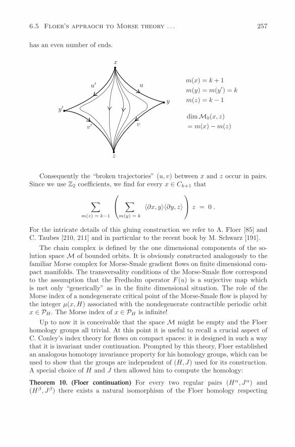
6.5 Floer’s appraoch to Morse theory . . . 257
has an even number of ends.
x
uu′
yy′
vv′
z
m(x) = k + 1m(y) = m(y′) = k
m(z) = k − 1
dimM0(x, z)= m(x) − m(z)
Consequently the “broken trajectories” (u, v) between x and z occur in pairs.Since we use Z2 coefficients, we find for every x ∈ Ck+1 that
∑m(z) = k−1
∑
m(y) = k
〈∂x, y〉〈∂y, z〉
z = 0 .
For the intricate details of this gluing construction we refer to A. Floer [85] andC. Taubes [210, 211] and in particular to the recent book by M. Schwarz [191].
The chain complex is defined by the one dimensional components of the so-lution space M of bounded orbits. It is obviously constructed analogously to thefamiliar Morse complex for Morse-Smale gradient flows on finite dimensional com-pact manifolds. The transversality conditions of the Morse-Smale flow correspondto the assumption that the Fredholm operator F (u) is a surjective map whichis met only “generically” as in the finite dimensional situation. The role of theMorse index of a nondegenerate critical point of the Morse-Smale flow is played bythe integer µ(x,H) associated with the nondegenerate contractible periodic orbitx ∈ PH . The Morse index of x ∈ PH is infinite!
Up to now it is conceivable that the space M might be empty and the Floerhomology groups all trivial. At this point it is useful to recall a crucial aspect ofC. Conley’s index theory for flows on compact spaces: it is designed in such a waythat it is invariant under continuation. Prompted by this theory, Floer establishedan analogous homotopy invariance property for his homology groups, which can beused to show that the groups are independent of (H, J) used for its construction.A special choice of H and J then allowed him to compute the homology:
Theorem 10. (Floer continuation) For every two regular pairs (Hα, Jα) and(Hβ , Jβ) there exists a natural isomorphism of the Floer homology respecting
258 Chapter 6 The Arnold conjecture, Floer homology . . .
the gradingψβα : HF∗(M,Hα, Jα) −→ HF∗(M,Hβ , Jβ) .
Moreover, if (Hγ , Jγ) is another regular pair, then
ψαβ ψβγ = ψαγ and ψαα = id .
We see that the Floer homology FH∗(M,H, J) is independent of the regularpair (H, J) used in the construction of the connecting orbits of PH ; hence it is aninvariant of the underlying manifold (M,ω). We have a category whose objectsare the Floer homology groups associated with regular pairs (H, J) and whosemorphisms are the natural isomorphisms ψβα induced by regular homotopies asexplained below. In the terminology of C. Conley [54] such a category with uniquemorphisms is called a connected simple system.
We shall sketch the ideas of the proof which is again based on special solutionsof a P.D.E. and Fredholm theory. We follow the presentation in D. Salamon andE. Zehnder [190]. In order to construct a homomorphism ϕβα : C(M,Hα, Jα) →C(M,Hβ , Jβ), we choose a smooth homotopy Hαβ : R × S1 × M → R of Hamil-tonian functions together with a smooth homotopy of almost complex structuresJαβ : R × M → End (TM) such that Hαβ(s, t, x) and Jαβ(s, x) are independentof s for |s| sufficiently large and satisfy
lims→−∞
Hαβ (s, t, x) = Hα(t, x)
lims→+∞
Hαβ (s, t, x) = Hβ(t, x)(6.140)
andlim
s→−∞Jαβ (s, x) = Jα(x)
lims→+∞
Jαβ (s, t, x) = Jβ(x) .(6.141)
Recall that the space of almost complex structures compatible with ω is con-tractible. Given such a pair (Hαβ, Jαβ) of homotopies connecting the data onestudies the smooth solutions u(s, t), u : R × S1 → M of the P.D.E.
∂u
∂s+ J(s, u)
∂u
∂t+ ∇H(s, t, u) = 0(6.142)
which satisfy the asymptotic boundary conditions
lims→−∞
u(s, t) = xα(t) , lims→+∞
u(s, t) = xβ(t)(6.143)
where xα ∈ PHα and xβ ∈ PHβ .The solutions can be considered as flow lines of a time-dependent gradient
flow defined by the action functional ϕHs, Hs(t, x) = Hαβ(s, t, x) with respect to
the time-dependent metric determined by the almost complex structure Js. As
6.5 Floer’s appraoch to Morse theory . . . 259
before, a solution of bounded energy satisfies the boundary conditions. We shallabbreviate by
M(xα, xβ ,Hαβ, Jαβ)(6.144)
the set of smooth solutions u : R × S1 → M of (6.142) and (6.143). This setis analyzed locally by linearizing the equation in the direction of a vector fieldξ ∈ C∞(u∗TM) along u which leads to a linear operator F βα(u) : W k,p(u∗TM) →W k−1,p(u∗TM) between appropriate Sobolev spaces. For every smooth map u :R×S1 → M satisfying the boundary conditions (6.143) with xα, xβ nondegenerate,the operator F βα(u) is Fredholm and its index is computed as
Index F βα (u) = µ(xα,Hα) − µ(xβ,Hβ) .(6.145)
Moreover, for a regular homotopy from (Hα, Jα) to (Hβ , Jβ) the operator is surjec-tive. Here a pair (Hαβ, Jαβ) is called regular, if both pairs (Hα, Jα) and (Hβ , Jβ)are regular and if the linear operator F βα(u) is surjective for every solution uof (6.142) and (6.143) for every xα ∈ PHα and xβ ∈ PHβ . Floer proved [84, 85]that the set of regular homotopies connecting regular pairs is dense in the setof all smooth homotopies connecting (Hα, Jα) to (Hβ, Jα) with respect to theC∞ topology. (Floer carried out his proof for the analogous geometric problem ofLagrangian intersections.) It then follows that the space M(xα, xβ,Hαβ, Jαβ) ofconnecting orbits is a finite dimensional manifold and
dimM(xα, xβ,Hαβ , Jαβ) = µ(xα,Hα) − µ(xβ ,Hβ) .(6.146)
This allows us to construct a chain homomorphism
ϕβα = ϕ(Hαβ , Jαβ) : Ck(M,Hα) → Ck(M,Hβ)
by counting the connecting orbits modulo 2 between periodic solutions having thesame index
ϕβα (xα) =∑
µ(xβ,Hβ)=k
〈ϕβα (xα), xβ〉xβ ,(6.147)
where µ(xα,Hα) = k and where 〈ϕβαxα, xβ〉 is the number of solutions modulo 2.One can show that for every regular homotopy this linear map ϕβα is a chain
homomorphisms, i.e., satisfies ∂βϕβα = ϕβα∂α. Moreover, it respects the grading.It, therefore, induces a natural homomorphism ψβα of Floer homology, whichturns out to be independent of the choice of the homotopy (Hαβ , Jαβ). Moreprecisely one shows that for two regular homotopies (Hαβ
0 , Jαβ0 ) and (Hαβ
1 , Jαβ1 )
from (Hα, Jα) to (Hβ , Jβ), the associated chain homomorphisms ϕβα0 and ϕβα
1 arechain homotopy equivalent. This finishes our sketch of Theorem 10.
Finally, in order to compute the homology, Floer used the continuation theoremand connected a regular pair (Hα, Jα) with a very special pair (H, J), whose Floerhomology agrees with the homology of the Morse complex defined by the gradientflow of the function H : M → R on the underlying manifold M .
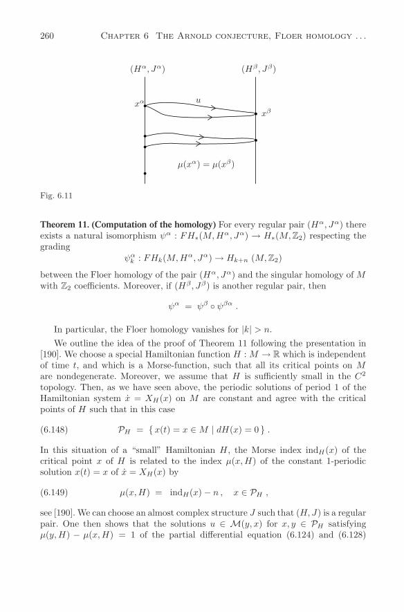
260 Chapter 6 The Arnold conjecture, Floer homology . . .
(Hα, Jα) (Hβ , Jβ)
xα u
xβ
µ(xα) = µ(xβ)
Fig. 6.11
Theorem 11. (Computation of the homology) For every regular pair (Hα, Jα) thereexists a natural isomorphism ψα : FH∗(M,Hα, Jα) → H∗(M, Z2) respecting thegrading
ψαk : FHk(M,Hα, Jα) → Hk+n (M, Z2)
between the Floer homology of the pair (Hα, Jα) and the singular homology of Mwith Z2 coefficients. Moreover, if (Hβ, Jβ) is another regular pair, then
ψα = ψβ ψβα .
In particular, the Floer homology vanishes for |k| > n.We outline the idea of the proof of Theorem 11 following the presentation in
[190]. We choose a special Hamiltonian function H : M → R which is independentof time t, and which is a Morse-function, such that all its critical points on Mare nondegenerate. Moreover, we assume that H is sufficiently small in the C2
topology. Then, as we have seen above, the periodic solutions of period 1 of theHamiltonian system x = XH(x) on M are constant and agree with the criticalpoints of H such that in this case
PH = x(t) = x ∈ M | dH(x) = 0 .(6.148)
In this situation of a “small” Hamiltonian H, the Morse index indH(x) of thecritical point x of H is related to the index µ(x,H) of the constant 1-periodicsolution x(t) = x of x = XH(x) by
µ(x,H) = indH(x) − n , x ∈ PH ,(6.149)
see [190]. We can choose an almost complex structure J such that (H, J) is a regularpair. One then shows that the solutions u ∈ M(y, x) for x, y ∈ PH satisfyingµ(y, H) − µ(x,H) = 1 of the partial differential equation (6.124) and (6.128)

6.5 Floer’s appraoch to Morse theory . . . 261
are also independent of the time t. Hence setting u(s, t) = γ(s), they satisfy thegradient equation
dγ
ds+ ∇H
(γ(s)
)= 0 on M ,(6.150)
and the boundary conditions γ(s) → y as s → −∞ and γ(s) → x as s → +∞.These solutions agree with the 1-dimensional connecting orbits of the Morse-Smalegradient flow x = −∇H(x) for which
M(y, x) = Wu(y) ∩ W s(x) ,(6.151)
whenever ind F (u) = indH(y)− indH(x) = 1. Hence, the chain complex C(M,H)agrees with the familiar Morse complex, in which Ck(H) = x ∈ M |dH(x) = 0and indH(x) = k and where the boundary operator ∂k = ∂k(H, J) : Ck → Ck−1
defined above counts the connecting orbits (mod 2) of the gradient flow on M . Itis well-known, that its homology groups
H Mk(M,H, J) =ker ∂k
im ∂k+1(6.152)
agree with the singular homology of M
H Mk(M,H, J) ∼= Hk(M, Z2) .(6.153)
For a proof we refer to D. Salamon [188] and to the recent monograph by M.Schwarz [191] in which he develops a Morse homology theory on finite dimensionalmanifolds based on the trajectory spaces of Morse functions. We see in view of(6.149) that Floer’s chain complex for our special symplectic manifold (M,ω)agrees with the familiar Morse complex of a gradient flow of a function, the gradingbeing shifted by n:
H Fk(M,H, J) ∼= H Mk+n(M,H, J) ∼= Hn+k(M, Z2) .(6.154)
Consequently, Floer’s connecting orbits of nondegenerate periodic solutions canserve as a model for the homology of the underlying manifold. We conclude, inparticular, that ∑
x∈PH
tµ(x,H) = P (t,M)t−n + (1 + t)Q(t) .(6.155)
This Morse equation relates the nondegenerate contractible periodic solutions x ∈PH having indices µ(x, H) ∈ Z to the topology of M described by the Poincarepolynomial P (t,M). Recall that we posed the assumptions ω|π2 = 0 = c1|π2 on(M,ω). In case of a time-independent and small Morse function H, the equation(6.155) becomes the familiar Morse equation∑
∇H(x)=0
tm(x) = P (t,M) + (1 + t)Q(t)(6.156)
which relates the critical points of the function H to the Poincare polynomialP (t,M). In particular, we conclude from (6.155)
262 Chapter 6 The Arnold conjecture, Floer homology . . .
Theorem 12. (Floer) Assume the compact symplectic manifold (M,ω) satisfiesω|π2(M) = 0 and c1|π2(M) = 0, assume the time periodic Hamiltonian vectorfield x = XH(x) on M possesses nondegenerate 1-periodic solutions only. Thentheir number is at least the sum of the Betti numbers SB(M, Z2) of M .
For example π2(T 2n) = 0 so that every symplectic torus (T 2n, ω) meets theassumption of the theorem. Actually Floer proved in [85] a more general result,assuming merely that (M,ω) a monotone in the sense that
∫
S2
u∗c1 = λ
∫
S2
u∗ω ,(6.157)
for every sphere u : S2 → M , with a constant λ > 0.More recently, H. Hofer and D. Salamon succeeded, [119], in defining the Floer
homology groups under the assumption that
ω(A) ≤ 0 for every A ∈ π2(M) satisfying 3 − n ≤ c1(A) < 0 ,(6.158)
and to compute them in the cases c1|π2(M) = 0 and N ≥ 12 dim(M), where
NZ = c1(π2(M)) ⊂ Z, proving the Arnold conjecture in these cases. They demon-strate that the Floer groups form a module over Novikov’s ring of generalizedLaurent series. Such a ring was introduced by S. Novikov in his generalization ofMorse theory for closed one-forms [170]. Under the assumption (6.158) the ob-tained theory is a Novikov type variant of Floer homology. Modifying the ideas ofHofer and Salamon, K. Ono [172] gave a modified construction of Floer’s homologytheory, again under the assumption (6.158), which can be computed without addi-tional hypothesis. It turns out that for a suitable coefficient field these Floer groupsare isomorphic to the singular homology groups of the manifold establishing, inparticular, the Arnold conjecture for the dimension 2, 4 and 6 in which (6.158) isvacuous. Manifolds meeting the condition (6.158) have the property used in theproof that, for a generic almost complex structure, there is no holomorphic sphereof negative Chern number.
The Arnold conjecture for a general compact symplectic manifold with dimM ≥ 8 is still open.
It should be mentioned that the Floer homology groups HF∗ can be definedfor integer coefficients Z (instead of Z2) and, therefore, for every Abelian group.In order to do this one has to assign an integer +1 or −1 to every connecting orbitu ∈ M(y, x) whenever µ(y) − µ(x) = 1. However, the determination of such anorientation is quite subtle and requires a consistent orientation of the moduli spacesM(y, x) for which we refer to A. Floer and H. Hofer [89]. Thus all the statementsdescribed above are true not only for Z2 coefficients but for Z coefficients as well.
The 1-periodic solutions of x = XH(x) on M correspond in a one-to-one wayto the fixed points of the Hamiltonian map ψ1 which is the time-1 map of theflow generated by the Hamiltonian vector field. Since M is compact one should
6.5 Floer’s appraoch to Morse theory . . . 263
expect, in view of Poincare’s recurrence theorem, in addition to these fixed pointsan abundance of periodic points having large periods. Indeed, if one of the fixedpoints is of general elliptic type as explained in the introduction, then it is a clusterpoint of other periodic points whose prime periods tend to infinity. This followssimply by the Birkhoff-Lewis theorem, a local theorem for the proof of which werefer to J. Moser [164]. Unfortunately, our global approach to the existence of thefixed points gives only little information about their nature and, in particular,no information about their nonlinear Birkhoff invariants required to deduce theperiodic points nearby. We shall show next under additional assumptions on the1-periodic solutions that infinitely many periodic solutions are deduced from theFloer homology. A 1-periodic solution x(t) = x(t + 1) can be considered as a τ -periodic solutions x(t) = x(t + τ) for every integer τ ∈ N, which is then calledthe τ -iterated solution of x and denoted by xτ . We call a 1-periodic solution xstrongly nondegenerate if all its iterates xτ are nondegenerate, i.e., if
det(1 − ψτ (x(0))
)= 0
for all positive integers τ , not only for τ = 1.
Theorem 13. Assume the compact symplectic manifold (M,ω) satisfies ω|π2 = 0and c1|π2 = 0 and assume H : S1 × M → R is a smooth Hamiltonian so that allthe contractible 1-periodic solutions of the Hamiltonian system are strongly non-degenerate. Then there are infinitely many contractible periodic solutions havinglarge integer periods.
This is a special case of a more general statement proved by D. Salamon andE. Zehnder in [190] which requires merely that the 1-periodic solutions x(t) =x(t+1) are weakly nondegenerate, i.e., they possess at least one Floquet multipliernot equal to 1 so that σ(dψ1(x(0))) = 1. The condition on π2(M) cannot beremoved as is demonstrated by the example of a rotation on M = S2 with irrationalfrequency (Fig. 6.12).
This is a Hamiltonian map, but has only two periodic points, namely thestrongly nondegenerate fixed points at the north and the south pole.
In sharp contrast to this example, an area preserving diffeomorphism of S2
having ≥ 3 fixed points, has automatically infinitely many periodic points. Thisstriking phenomenon has been discovered by J.M. Gamboudo and P. Le Calvez[103] and J. Franks [96]. One is tempted to conjecture that every Hamiltonianmap on a compact symplectic manifold (M,ω) possessing more fixed points thannecessarily required by the V. Arnold conjecture possesses always infinitely manyperiodic points. Similarly one could expect, that a compact and strictly convexhypersurface S ⊂ R
4, carries either 2 or ∞ many closed characteristics.
Theorem 13 is an easy consequence of the Floer homology. We make use ofthe fact proved in [190], that for the index µ(x,H) of a strongly nondegenerate
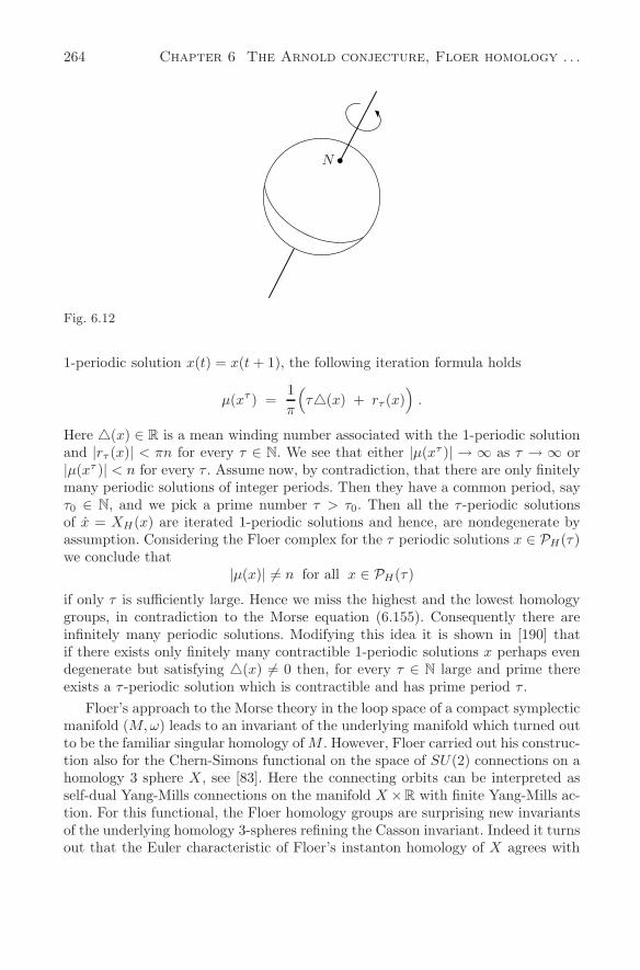
264 Chapter 6 The Arnold conjecture, Floer homology . . .
N
Fig. 6.12
1-periodic solution x(t) = x(t + 1), the following iteration formula holds
µ(xτ ) =1π
(τ(x) + rτ (x)
).
Here (x) ∈ R is a mean winding number associated with the 1-periodic solutionand |rτ (x)| < πn for every τ ∈ N. We see that either |µ(xτ )| → ∞ as τ → ∞ or|µ(xτ )| < n for every τ . Assume now, by contradiction, that there are only finitelymany periodic solutions of integer periods. Then they have a common period, sayτ0 ∈ N, and we pick a prime number τ > τ0. Then all the τ -periodic solutionsof x = XH(x) are iterated 1-periodic solutions and hence, are nondegenerate byassumption. Considering the Floer complex for the τ periodic solutions x ∈ PH(τ)we conclude that
|µ(x)| = n for all x ∈ PH(τ)
if only τ is sufficiently large. Hence we miss the highest and the lowest homologygroups, in contradiction to the Morse equation (6.155). Consequently there areinfinitely many periodic solutions. Modifying this idea it is shown in [190] thatif there exists only finitely many contractible 1-periodic solutions x perhaps evendegenerate but satisfying (x) = 0 then, for every τ ∈ N large and prime thereexists a τ -periodic solution which is contractible and has prime period τ .
Floer’s approach to the Morse theory in the loop space of a compact symplecticmanifold (M,ω) leads to an invariant of the underlying manifold which turned outto be the familiar singular homology of M . However, Floer carried out his construc-tion also for the Chern-Simons functional on the space of SU(2) connections on ahomology 3 sphere X, see [83]. Here the connecting orbits can be interpreted asself-dual Yang-Mills connections on the manifold X ×R with finite Yang-Mills ac-tion. For this functional, the Floer homology groups are surprising new invariantsof the underlying homology 3-spheres refining the Casson invariant. Indeed it turnsout that the Euler characteristic of Floer’s instanton homology of X agrees with
6.6 Symplectic homology 265
double the Casson invariant. We shall not discuss these developments in topologyhere and refer instead to J.C. Sikorav’s Seminaire Bourbaki [199] in 1990. Floer’sinstanton homology was extended to general oriented 3-manifolds by K. Fukayain [102]. Recent developments on instanton homology are presented in the Floermemorial volumes [120].
6.6 Symplectic homology
In Chapter 3 we introduced the special symplectic capacity c0(M,ω) dynamicallyin terms of Hamiltonian systems. The existence proof was based on a distinguishedcritical point of the action functional. This critical point represents a particularperiodic orbit and the question arises whether the structure of all critical pointstogether with their connecting orbits leads to a more subtle symplectic invariantwhich is not necessarily a number anymore. Indeed, combining the construction ofthe capacity c0 with Floer’s homology construction in the loop space H. Hofer, andA. Floer established in [90] a symplectic homology theory. Our aim is to sketch,without proofs, this theory which is not yet in its final form.
We first recall the setting from the previous section and consider a symplecticmanifold (M,ω) satisfying π2(M) = 0, for simplicity. By Ω(M) we denote theset of parameterized contractible loops x : S1 → M . If H : S1 × M → R is atime-periodic Hamiltonian, the action functional ϕH : Ω(M) → R is defined by
ϕH(x) = −∫
D
x∗ω +
1∫
0
H(t, x(t)
)dt .
Here x : D → M is an extension of x to the closed unit disc D satisfying x|∂D = x.The critical points of ϕH are the contractible 1-periodic solutions of the Hamilto-nian vector field x = XH(x) on M . We shall assume that all of them are nonde-generate and denote this finite set by PH . By C(M,H) we denote the vector spaceover Z2 generated by PH to be
C = ⊕Ck , Ck(M,H) = spanZ2
x ∈ PH |µ(H, x) = k .
The grading is determined by the index µ(H, x) ∈ Z intrinsically associated to thenondegenerate periodic solutions x ∈ PH . For a generic almost complex structure Jassociated with ω there exists a boundary operator ∂k = ∂k(M,H, J) : Ck → Ck−1.It is defined by counting (mod 2) the connecting orbits M(x−, x+,H, J) whichconnect periodic solutions of index difference µ(H, x−) − µ(H, x+) = 1. The pair(C, ∂) is a chain complex and we denote by
F∗(M,H, J) =ker ∂
im ∂
the Floer homology of the generic pair (H, J). Turning now to the constructionof the symplectic homology of (M,ω), we first make the observation that for a
266 Chapter 6 The Arnold conjecture, Floer homology . . .
fixed generic pair (H, J) there exists an additional filtration of the Floer complexdefined by the values of the functional ϕH on Ω(M). We define for a ∈ R ∪ ∞the graded free groups
Ca(M,H) =⊕k∈Z
Cak
Cak = spanZ2
x ∈ PH |µ(H, x) = k and ϕH(x) < a .
Assume now that u is a connecting orbit in M(x−, x+,H, J) and denote by us ∈ Ωthe loops us(t) = u(s, t). By the variational structure, ϕH(x+) ≤ ϕH(us) ≤ϕH(x−), hence the periodic orbits lying between two different levels together withtheir connecting orbits constitute a subcomplex of the Floer complex. More pre-cisely ∂ = ∂(H, J) satisfies
∂ : Cak → Ca
k−1.
Therefore, defining for −∞ < a ≤ b ≤ ∞, the quotient group by
C [a,b)(H, J) =Cb(H, J)Ca(H, J)
,(6.159)
then the boundary map induces a boundary operator ∂k : C[a,b)k → C
[a,b)k−1 , and we
can define
F[a,b)k (H, J) =
ker(∂k)im (∂k+1)
.(6.160)
Yet, this Floer homology group depends on the choice of a generic pair (H, J) andis not an invariant of M . The aim is to construct a directed set of very specialgeneric pairs, so that the directed limit of the corresponding groups defines asymplectic invariant of M . The class of admissible Hamiltonians in a generic pairis prompted by the class used in the construction of c0(M,ω) in Chapter 3.
We sketch this construction for compact symplectic manifolds (M,ω) possiblyhaving a boundary ∂M . In the case that ∂M = ∅ we shall assume that ∂M isof contact type as defined above. Equivalently, this requires that there exists a1-form λ on ∂M satisfying dλ = ω on ∂M and λ(x, ξ) = 0 for all nonvanishingξ ∈ Tx(∂M) for which ω(ξ, η) = 0 for all η ∈ Tx(∂M). Moreover, we assume forsimplicity, as above, that π2(M) = 0. By H we denote the collection of all smoothand time-periodic Hamiltonian functions H : S1 × M → R satisfying
supp(H) is compact in S1 × (M\∂M) and H(S1 × M) ⊂ (−∞, 0].(6.161)
Clearly this condition implies that there are many periodic solutions x of XH on Mwhich are degenerate and satisfy ϕH(x) = 0. In addition to (6.161) we, therefore,require that all contractible periodic solutions x of XH satisfying ϕH(x) < 0are nondegenerate. Consequently, if −∞ ≤ a ≤ b ≤ 0 we can define as abovethe relative Floer groups F [a,b)(H, J). Here, however, not every J is admissible.
6.6 Symplectic homology 267
The J has to be chosen in such a way that every solution u : R × S1 → M inM(x−, x+,H, J) stays away from the boundary, i.e., u(R×S1) ⊂ M\∂M , providedx− and x+ are contained in M\∂M . Such admissible J ’s do exist; the boundary∂M is then called J-pseudo convex in the sense of D. McDuff [154]. We shall calla pair (H, J) satisfying the above conditions admissible and introduce in the setof admissible pairs a partial ordering, by defining (this is not a typing error)
(H, J) ≤ (K, J) ⇐⇒ H(t, x) ≥ K(t, x)
for all (t, x) ∈ S1 × M . For such pairs one can define a monotone homotopy. Itconsists of a pair (L, J), where L : R×S1×M → R and where the almost complexstructure J(s, t, x) is adapted to the symplectic form ω. Moreover, L = H, J = Jfor s → −∞ while L = K, J = J for s → +∞, and ∂L
∂s ≤ 0. Given a monotonehomotopy for (H, J) ≤ (K, J) one considers the partial differential equations foru : R × S1 → M :
∂u
∂s+ J(s, t, u)
∂u
∂t+ (∇JL) (s, t, u) = 0
u(s, ·) → x ∈ PH (s → −∞)
u(s, ·) → y ∈ PK (s → +∞).
Using the monotonicity assumption we conclude that ϕK(y) ≤ ϕH(x). This im-plies that the boundary operator ∂ preserves the real filtration; this was the reasonfor the monotonicity assumption. Proceeding as in Floer’s construction, the com-binatorics of the set of solutions is used to construct a natural homomorphism
F [a,b)(H, J) → F [a,b)(K, J)
of Z2 vector spaces, which is independent of the chosen generic monotone homo-topy. The partial ordering ≤ turns the set of admissible pairs (H, J) into a directedset, since given (H1, J1) and (H2, J2), there exists an admissible pair (H, J) satis-fying
(Hj , Jj) ≤ (H, J) for j = 1, 2.
Hence we may pass to the limit obtaining the symplectic homology group
SM[a,b) = dir. lim F [a,b)(H, J).
In addition, if U ⊂ M is an open subset, and if HU consists of those admissiblepairs (H, J) which are restricted by the requirement that supp(H) ⊂ S1×(U\∂M),we may take the directed limit over HU and obtain a symplectic homology groupof U defined by
SM[a,b) (U) : = dir. lim
HU
F [a,b) (H, J).
We next list some of the properties of these groups known so far. It can be shownthat there are natural homomorphisms of Z2 vector spaces
SM[a,b) (U) → SM
[a,b).
268 Chapter 6 The Arnold conjecture, Floer homology . . .
Moreover, the short exact sequence 0 → F [a,b)(H, J) → F [a,c)(H, J) →F [b,c)(H, J) → 0, for −∞ ≤ a ≤ b ≤ c ≤ 0, gives rise to an exact trianglea,b,c(U) of symplectic homology groups:
S[a,b) (U) −→ S[a,c) (U)
∂
S[b,c) (U).
Given a symplectic diffeomorphism ψ : M → M we can define for any admissiblepair (H, J), with H ∈ HU , a new admissible pair (Hψ , Jψ) as follows:
Hψ(t, x) = H(t, ψ−1(x)
)
Jψ(x) = Tψ(ψ−1(x)
)J(ψ−1(x)
)Tψ−1(x).
This is used to show that ψ induces a natural isomorphism
ψ# : SM[a,b) (U)
∼=−→ SM[a,b)
(ψ(U)
).
If U ⊂ V then the inclusion map induces a homomorphism
σV,U : SM[a,b) (U) → SM
[a,b) (V ) .
If ψ : M → M is a symplectic diffeomorphism satisfying ψ(U) ⊂ V , we define theinduced map ψ∗ by
ψ∗ = σV,ψ(U) ψ# : SM[a,b) (U) → SM
[a,b) (V ).
Then if ϕ : M → M is another symplectic diffeomorphism satisfying ϕ(V ) ⊂ W ,one can prove
(ϕ ψ)∗ = σW,ϕψ(U) (ϕ ψ)#
=(σW,ϕ(V ) ϕ#
)
(σV,ψ(U) ψ#
)
= ϕ∗ ψ∗.
Moreover, the identity map of M induces the identity map id: SM[a,b)(U)→SM
[a,b)(U).The most useful property is the isotopy invariance formulated as follows: if ψs :M → M for 0 ≤ s ≤ 1 is a smooth family of symplectic diffeomorphisms satisfyingψs(U) ⊂ V for all s, then (ψs)∗ : SM
[a,b)(U) → SM[a,b)(V ) is independent of s.
It is rather difficult to compute the symplectic homology groups sketched aboveand we refer to [50] for computations and applications. It is not surprising anymorethat the homology groups are related to distinguished periodic orbits, which siton or near the boundary of a domain. This is illustrated by the theorem below.
6.6 Symplectic homology 269
We consider a compact symplectic manifold (M,ω) with boundary ∂M = ∅which is exact symplectic, i.e., ω = dλ for a 1-form λ. We assume the boundaryto be of contact type with respect to λ. Then we can define the action spectrumσ(∂M) ⊂ R as follows: σ(∂M) = |
∫x
λ|, where x is a periodic solution of the Reeb
vector field on ∂M, note that iterated solutions are also considered, in particular,k · σ(∂M) ⊂ σ(∂M) for k ∈ N.
Theorem 14. (K. Cieliebak, A. Floer, H. Hofer and K. Wysocki [52]) Consider twoexact symplectic and compact manifolds (M,dλ) and (N, dτ) with boundaries ∂Mand ∂N of contact type with respect to λ and τ . Assume there exists an exactsymplectic diffeomorphism
ϕ :
M →
N
(i.e., ϕ∗τ − λ = dF for a smooth function F :
M → R). If the periodic solutionson ∂M and ∂N and all their iterates are nondegenerate, then
σ(∂M) = σ(∂N ).
Examples by Ya. Eliashberg and H. Hofer [75] demonstrate that under the as-sumptions of the theorem, the flows on ∂M and ∂N are not necessarily conjugated,so that ϕ cannot be extended to a symplectic diffeomorphism M → N .
The proof of Theorem 14 is based on the following nontrivial fact [52]. Letα < 0 and define
dM (α) =12
limε→0
dim S[α−ε,α+ε)M (
M).
Then dM (α) = 0 if −α /∈ σ(∂M) and
dM (α) = #
periodic solutions x on ∂M with action |∫
x
λ| = −α
.
Since S[a,b)M (
M ) = S
[a,b)N (
N ) for all a < b, we conclude dM(α) = dN (α) so that the
theorem follows. For the intricate details of the proof and for applications of thisresult, we refer to the forthcoming paper [52].
By computing the homology groups one also proves a conjecture by Gromovon the symplectic classification of open polydiscs. Define for r = (r1, r2, . . . , rn),where 0 < r1 ≤ r2 ≤ · · · ≤ rn, the polydisc D(r) = B2(r1) × · · · × B2(rn).
Theorem 15. The open polydiscs D(r) and D(r′) are symplectomorphic if and onlyif r = r′, assuming r and r′ are ordered.
We recall that we have proved this statement in Chapter 2 for the special casen = 2. The proof was based on two symplectic invariants: the volume and a ca-pacity. The proof for n ≥ 2 follows with other applications, in [52]. The details ofthe above construction of the symplectic homology are carried out in K. Cieliebak,
270 Chapter 6 The Arnold conjecture, Floer homology . . .
A. Floer and H. Hofer [51] where also possible extensions of this theory are out-lined. The proof is based on the action principle in the loop space of symplecticmanifolds and combines the construction of the dynamical capacity of Chapter3 and the construction of the Floer homology, with an additional real filtration.An alternate more recent construction of a symplectic homology theory for opensubsets of (R2n, ω0) can be found in L. Traynor [212]; the construction is basedon the generating function approach in a finite dimensional setting introduced in[218] by C. Viterbo.
Concluding remarks. As already pointed out in the introduction we have selectedonly a few and rather elementary topics in symplectic geometry and explainedthem in detail. We would, therefore, like to mention some additional literature.There is a whole sequence of relative symplectic capacities for subsets in (R2n, ω0)in the framework of symplectic diffeomorphisms defined on all of R
2n constructedby I. Ekeland and H. Hofer in [68]. These capacities have an outer regularityproperty, in contrast to the intrinsically defined dynamical capacity of Chapter3 which has an inner regularity property. Quite recently S. Kuksin extended in[130] the capacity concept to some special infinite dimensional Hamiltonian sys-tems defined by partial differential equations, e.g. nonlinear string equation onS1, some nonlinear Schrodinger equations on Tn. He proved, in particular, a nonsqueezing result for the flows of such systems. The construction of the capacity isbased on a Galerkin approximation using the finite dimensional capacities intro-duced in Chapter 3. Kuksin’s result prompted a non squeezing result for a veryspecial nonlinear Schrodinger equation on S1, whose flow maps are not compactperturbations of linear maps in the symplectic Hilbert space, see J. Bourgain [31].Extending the embedding capacity, called the Gromov-width in Chapter 2, onecan define, for every integer k, a new capacity as follows: one takes k symplecticembeddings of equal balls B(r) having disjoint images in (M,ω) and determinesan upper bound of the radius r. This leads to the symplectic packing problemrelated to algebraic geometry studied by D. McDuff and L. Polterovich in [155];for interesting packing constructions we point out L. Traynor [213]. The intrin-sic L∞-geometry on the group of compactly supported Hamiltonian mappings of(R2n, ω0) described in Chapter 5 has been extended to general symplectic mani-folds by F. Lalonde and D. McDuff in [134] and [135]. It turns out that the cornerstone of this geometry, namely the energy-capacity inequality, is equivalent to thenon squeezing theorem. Conjugate points on geodesics in the Hofer metric havein the meantime been investigated by I. Ustilovsky in [214]. For a survey on theseinteresting developments we point out F. Lalonde [133].
As already emphasized, the V.I. Arnold conjecture about fixed points of Hamil-tonian mappings is open for general compact symplectic manifolds of dim M ≥ 8.For a survey on Floer’s contributions to this problem we refer to D. McDuff [153]and to the Floer memorial volume [120]. Recently an analogue of the Arnoldconjecture for symplectic mappings ϕ which are not necessarily Hamiltonian butisotopic to the identity through symplectic diffeomorphisms has been studied by

6.6 Symplectic homology 271
Le Hong Van and Kaoru Ono [137]. They prove for compact manifolds satisfyingc1|π2(M) = λω|π2(M) (λ ≥ 0) assuming that all the fixed points are nondegener-ate, that the number of fixed points of ϕ is at least the sum of the Betti-numbersof the Novikov homology over Z2 associated to the Calabi-invariant α of ϕ, Nov(α). In the special case of the torus T 2n considered in Chapter 6, Nov (α) = 0 ifα = 0, so that one obtains nothing new for the torus.
Finally, for an abundance of exciting developments and discoveries in sym-plectic geometry not treated in our book, e.g. pseudo-holomorphic spheres, fillingtechniques, Lagrangian intersections, contact geometry, examples of symplecticmanifolds, and so on, we refer to the forthcoming books by D. McDuff and D. Sala-mon [156], M. Audin, J. Lafontaine [13], B. Aebischer, M. Borer, Ch. Leuenberger,M. Kalin, H.M. Reimann [3] and C. Abbas, H. Hofer [1].
Appendix
A.1 Generating functions of symplectic mappings in R2n
We shall start with the very useful observation that every symplectic map canlocally be represented in terms of a single scalar function, a so-called generatingfunction. This will be used in Appendix 2 to prove the Arnold-Jost theorem con-cerning the construction of so-called action-angle coordinates in integrable systems.Such Hamiltonian systems are characterized by the property of having sufficientlymany integrals so that, as we shall show, the task of solving (or “integrating”) thedifferential equations becomes trivial, after a global symplectic transformation.
All the considerations in section A.1 are local in nature. We consider a sym-plectic mapping u : (ξ, η) → (x, y) in (R2n, ω0) represented by
x = a(ξ, η)
y = b(ξ, η) .(A.1)
If we assume
det(aξ) = 0 ,(A.2)
then, locally, the first equation in (A.1) can be solved for ξ = α(x, η) and insertingthis solution into the second equation in (A.1) we find the following equivalentrepresentation of the map u:
ξ = α(x, η)
y = β(x, η) ,
where β(x, η) = b(α(x, η), η) and
det(αx) · det(aξ) = 1 .
The advantage of scrambling the variables in this seemingly ugly manner is thatthe condition for u to be symplectic is much easier to express in terms of α and βthan in terms of a and b. We shall show that under the condition (A.2) the mapu is symplectic if and only if there exists a scalar function W = W (x, η) with
ξ = α(x, η) = ∂∂η W (x, η)
y = β(x, η) = ∂∂xW (x, η) .
(A.3)
H. Hofer and E. Zehnder, Symplectic Invariants and Hamiltonian Dynamics, 273Modern Birkhäuser Classics, DOI 10.1007/978-3-0348-0104-1, © Springer Basel AG 2011
274 Appendix
Hence (β, α) is the gradient of a function. To prove this statement we consider onR
4n, having the coordinates (ξ, η, x, y) ∈ R4n, the one-form,
σ =n∑
j=1
yjdxj + ξjdηj ,
whose exterior derivative is the two-form
dσ =n∑
j=1
dyj ∧ dxj −n∑
j=1
dηj ∧ dξj .
Introducing the embeddings i and j: R2n → R
4n by
i : (x, η) →(α(x, η), η, x, β(x, η)
)
j : (ξ, η) →(ξ, η, a(ξ, η), b(ξ, η)
)
and defining the local diffeomorphism ϕ : R2n → R
2n by (x, η) → (ξ, η) =(α(x, η), η), we have i = j ϕ. Consequently,
d(i∗σ) = i∗ dσ = ϕ∗(j∗ dσ)
= ϕ∗(u∗ω0 − ω0) .
If u is symplectic, that is u∗ω0 − ω0 = 0, then i∗σ is closed and, therefore, locallyexact, such that
i∗σ(x, η) =n∑
j=1
βj(x, η)dxj + αj(x, η)dηj
= dW (x, η) =n∑
j=1
Wxj(x, η)dxj + Wηj
(x, η)dηj
for a function W = W (x, η). From this identity we read off (A.3). We can reverseall the steps and hence have proved:
Proposition 1. Every symplectic mapping u as in (A.1) satisfying (A.2) can locallybe represented in the implicit form
ξ = Wη(x, η)
y = Wx(x, η) ,(A.4)
where det(Wxη) = 0. Conversely, any smooth function W = W (x, η) satisfyingthis inequality defines implicitly by (A.4) a symplectic mapping u near a point.
The function W (x, η) is called a generating function of the symplectic map u.The proposition shows that a symplectic map u satisfying (A.2) can locally be
A.1 Generating functions of symplectic mappings in R2n 275
described in terms of a single function. For example, the identity map correspondsto W (x, η) = 〈x, η〉. Thus every function W ,
W (x, η) = 〈x, η〉 + w(x, η) ,
w being small together with its first two derivatives, defines a symplectic mappingnear the identity, and all such mappings can, locally, be parameterized by func-tions. Of course, other generating functions can be constructed. If we single out(x, ξ) as independent variables, where we assume
det(aη) = 0,(A.5)
instead of (A.2) we can represent the map u in (A.1) locally in the implicit form
η = − Vξ(ξ, x)
y = Vx(ξ, x), det(Vxξ) = 0(A.6)
with a generating function V (ξ, x). The proof proceeds as above, but starts withthe one-form on R
4n given by σ = y dx − η dξ, in short notation. For example,the identity map violates conditions (A.5) but satisfies (A.2) while the symplecticrotation
x = η , y = −ξ
satisfies (A.5) but violates (A.2). However, for every symplectic mapping thereis some generating function representing it, as we shall prove next. The so-calledgroup of elementary symplectic transformations of (R2n, ω0) is generated by therotation
x1 = η1 , xk = ξk , k ≥ 2 .
y1 = −ξ1 yk = ηk
and the mappings
xj = ξπ(j) , yj = ηπ(j) , j = 1, 2, . . . , n,
with a permutation π of the integers (1, 2, . . . , n). All these mappings are sym-plectic and can be represented by symplectic matrices which we abbreviate byE.
Proposition 2. Let U be a linear symplectic map of (R2n, ω0). Then there exists anelementary symplectic transformation E satisfying
U · E =
(A B
C D
)and detA = 0 .
With U and UT is a symplectic matrix, hence Proposition 2 follows immediatelyfrom
276 Appendix
Lemma 1. Let A respectively B be two n × n matrices having column vectorsaj respectively bj ∈ R
n for 1 ≤ j ≤ n. Assume that the rank of the 2n × nmatrix (A,B) is equal to r. If ABT = BAT then there are r different indicesjp ∈ 1, 2, . . . , n such that there are column vectors vp = ajp
or vp = bjp, which
are linearly independent.
Proof. The following argument is due to C. de Boor. Choose I ⊂ 1, 2, . . . , n suchthat ajj∈I are linearly independent and Im(A) = spanaj |j ∈ I. It is sufficientto show that
Im(B) ⊂ Im(A) + spanbs | s /∈ I .(A.7)
Pick a basis cj of Rn satisfying 〈aj , ck〉 = δjk for j, k ∈ I. Then one computes, for
j ∈ I, thatBAT cj = bj +
∑s/∈I
dj(s)bs ,
where dj(s) is the s-th component of the vector AT cj . Since Im(BAT ) ⊂ Im(A),due to the assumption BAT = ABT , we conclude that bj , j ∈ I, belongs toIm(A)+ span bs, s /∈ I and so the claim (A.7) follows and the lemma is proved.
Applying Proposition 2 to a symplectic map u with Jacobian U at some point,we achieve the condition (A.2) to hold for u E with some elementary symplectictransformation E and thus find a local representation in terms of a generatingfunction near this point. To illustrate the use of generating functions we shalldetermine the most general symplectic map u in (A.1) for which
x = a(ξ)(A.8)
is prescribed, satisfies det(aξ) = 0, and is independent of η. Representing thedesired map u by a generating function V (ξ, y) in the form
x = Vy(ξ, y)
η = Vξ(ξ, y),
we find Vy(ξ, y) = a(ξ) and hence V (ξ, y) = 〈a(ξ), y〉 − v(ξ) or η = Vξ = aTξ y − vξ
and the explicit representation of u is
u :x = a(ξ)
y = (aTξ )−1
(η + vξ(ξ)
)(A.9)
where v = v(ξ) is an arbitrary scalar function. This is the most general symplecticmap u compatible with (A.8). For the special case that a = id we find
u :x = ξ
y = η + vξ(ξ) .(A.10)
A.1 Generating functions of symplectic mappings in R2n 277
In order to generalize these considerations we first recall a definition. If (M,ω) isany symplectic manifold, then the Poisson bracket of two functions F, G : M → R
is defined to be the function
F, G = −ω(XF , XG)(A.11)
where XF is the Hamiltonian vector field associated to the function F . ClearlyF, G = −G,F, and, since ω(XF , ·) = −dF , we have
F, G = dF (XG) = −dG(XF ) .(A.12)
A symplectic map u on M , i.e., u∗ω = ω, leaves the Poisson-bracket invariant:
F, G u = F u,G u .(A.13)
In order to verify this, recall the transformation formula for Hamiltonian vectorfields, u∗XG = (du)−1XG u = XGu if u∗ω = ω. Therefore F, G u =dF u(XG u) = d(F u)(u∗XG) = d(F u)(XGu) = F u,G u proving theclaim (A.13). Conversely, one verifies readily that a map u satisfying (A.13) for allfunctions F and G is necessarily a symplectic map. One verifies, moreover, easilythat for all functions F, G and H on M
[XF , XG] = XG,F(A.14)
and
F, G,H + H, F, G + G, H, F = 0 .(A.15)
Actually, it can be shown for a nondegenerate 2-form ω on M that the conditiondω = 0 is equivalent to each of the conditions (A.14) and (A.15), see, e.g., [167].
Locally in a Darboux chart of M i.e., in (R2n, ω0) the Poisson-bracket of twofunctions F = F (x, y) and G = G(x, y) is expressed as
F, G = 〈Fx, Gy〉 − 〈Fy, Gx〉 .(A.16)
The special coordinate functions (x, y) → xj , for example, satisfy xi, xj = 0.Hence, if u : (ξ, η) → (x, y) = (a(ξ, y), b(ξ, y)) is a symplectic map we con-clude from the invariance of the Possion brackets that ai, aj = 0, where xj =aj(ξ, η), 1 ≤ j ≤ n. Our aim is to prove the converse:
Theorem 1. (Liouville) Consider n functions aj = aj(ξ, η), 1 ≤ j ≤ n satisfying
(i) ai, aj = 0
(ii) rank (aξ, aη) = n.
Then there is a local symplectic diffeomeorphism u = (a, b),
x = a(ξ, η)
y = b(ξ, η) ,
extending the relation x = a(ξ, η).
278 Appendix
Proof. By applying an elementary symplectic transformation we may assume thatdet(aξ) = 0 and solve the equation x = a(ξ, η) for ξ = α(x, η). We shall provethat αη is symmetric as a consequence of the condition (i). Indeed this conditioncan be written as aξa
Tη − aηaT
ξ = 0. Multiplying this equation by a−1ξ from the
left and its transpose from the right we find aTη (aT
ξ )−1 − a−1ξ aη = 0, i.e., a−1
ξ aη issymmetric. On the other hand, differentiating the identity ξ = α(a(ξ, η), η) yields
1l = αx aξ and 0 = αx aη + αη ,
and consequently αη = −a−1ξ aη which is symmetric, as claimed. Therefore, locally,
there is a function W = W (x, η) with
α(x, η) = Wη(x, η) .
Moreover, det(Wxη) = det(αx) = (detaξ)−1 = 0, and hence W is a generatingfunction of the desired symplectic map u extending x = a(ξ, η). Corollary. If a0, a1, . . . an are (n + 1) functions for which
(i) aj , ak = 0 , j, k = 0, 1, . . . n
(ii) rank(ajξ, ajη
)j=1,2,...n
= n ,
then a0 can be expressed as a function of a1, . . . an. In particular, there are at mostn independent functions satifying (i).
Proof. Extending the relation x = a(ξ, η) by the theorem, we find a symplecticmap u for which a u(x, y) = x . Now set a0 u = f(x, y). Since the Poissonbracket is preserved under u we have 0 = aj , a0 = xj , f = fyj
so that f isindependent of y. Hence a0 = f(a1, . . . an) proving the corollary.
For further examples of generating functions we refer to the Notes on Dynam-ical Systems by J. Moser and E. Zehnder [167]. We turn now to a global versionof Liouville’s theorem.
A.2 Action-angle coordinates, the Theorem of Arnold and Jost
We consider a symplectic manifold (M,ω) of dim M = 2n.
Definition. A Hamiltonian vector field XH on M is called integrable (in the senseof Liouville) if there exist n functions Fj : M → R, 1 ≤ j ≤ n satisfying at everypoint of M :
(i) dF1, . . . dFn are linearly independent
(ii) Fi, Fj = 0 for all i, j .
(iii) H, Fj = 0 for all j .
A.2 Action-angle coordinates, the Theorem of Arnold and Jost 279
Introducing the map
F : M −→ Rn , F (x) =
(F1(x), . . . Fn(x)
)(A.17)
we conclude from (i) that the level sets
Nc = x ∈ M | F (x) = c , c ∈ Rn(A.18)
are n-dimensional submanifolds of M . The Hamiltonian vector fields XFjare lin-
early independent and, since dFi(XFj) = 0 in view of (ii), they span the tangent
space of Nc:TxNc = spanXFj
(x) | 1 ≤ j ≤ n ,
x ∈ Nc. We remark, moreover, that in view of ω(XFj, XFi
) = 0 we have ω(v, w) = 0for all pairs v, w ∈ TxNc. Hence Nc is a Lagrangian submanifold of M . By (iii),the functions Fj are all integrals of XH which is therefore tangent to the level setsNc so that the flow of XH leaves Nc invariant. Under an additional topologicalassumption on Nc, the flow can be determined explicitly for all times in view of thefollowing theorem which goes back to V. Arnold [12] in the special case M = R
2n.However, Arnold required an additional assumption which was removed by R. Jostin [126] who proved it in the general case.
Theorem 2. (Arnold-Jost) Let (M,ω) be a symplectic manifold of dim M = 2n.Assume there are n functions Fj satisfying (i) and (ii) at every point. Assume,moreover, that one of the level sets, say N = F−1(0) ⊂ M is compact and con-nected. Then
1) N is an embedded n-dimensional torus Tn.
2) There is an open neighborhood U of N in M which can be described by theaction and angle variables (x, y) in the following manner. If x = (x1, . . . , xn)are the variables on the torus Tn = R
n/Zn and y = (y1, . . . , yn) ∈ D1, where
D1 and D2 are some domains in Rn containing y = 0, then there exists a
diffeomorphism
ψ : Tn × D1 −→ U =⋃
c∈D2
(F−1(c) ∩ U
)
and a diffeomorphism µ : D2 → D1, with µ(0) = 0, such that
ψ∗ω =n∑
j=1
dyj ∧ dxj = ω0(A.19)
µ F ψ(x, y) = y .(A.20)
In particular, ψ maps the torus Tn×0 diffeomorphically onto F−1(0) = Nand the torus Tn × y onto Nc ∩ U where y = µ(c).
280 Appendix
Corollary: Any integrable Hamiltonian system given by H having the integrals Fj
is by the symplectic diffeomorphism ψ transformed into the following system on(Tn × D1, ω0):
H ψ(x, y) = h(y) ,(A.21)
where the Hamiltonian h depends on the integrals only and not on the anglevariables x.
Proof of the Corollary: In view of (A.13) the functions Fj ψ and therefore, by(A.20) also the coordinate functions yj , are integrals of H ψ, and hence
0 = H ψ, yj = h, yj =∂
∂xjh
so that h(x, y) = H ψ(x, y) does indeed not depend on the x variables. Consequently, on ψ−1(U) the transformed Hamiltonian system looks extremely
simple:
Xh : x =∂h
∂y(y) , y = 0 .
It is easily “integrated” with the solutions
x(t) = x(0) + t∂h
∂y
(y(0)
), y(t) = y(0)
hence the name “integrable systems”. Geometrically, every torus Tn×y in Tn×D2 is invariant under the flow ϕt of Xh and the restriction onto such a torus islinear:
ϕt | Tn × y : (x, y) → (x + tω, y)
where ω = ∂h∂y (y) ∈ R
n are the frequencies of this particular torus. We see that inthe open set U ⊂ M all the solutions of x = XH(x) are quasi-periodic.
Proof of Theorem 2. The proof proceeds in several steps. First we show that N isa torus. Second we introduce convenient coordinates (x, y) locally near a point pon N by means of Liouville’s theorem. Thirdly, these coordinates are extended toan open neighborhood of N by means of the flows of the Hamiltonian vector fieldsXFj
. Finally, the normalization of the periods requires an additional symplecticchange of variables to conclude the proof.
a) In order to prove the first statement of the theorem, we denote by ϕsj
j
the flow of XFj. Since [XFj
, XFi] is a Hamiltonian vector field with Hamiltonian
function Fi, Fj = 0, the vector fields XFjand hence also their flows do commute
and we abbreviate
ϕs = ϕs11 ϕs2
2 . . . ϕsnn , s = (s1, . . . , sn) ∈ R
n,(A.22)
A.2 Action-angle coordinates, the Theorem of Arnold and Jost 281
wherever it is defined. Since the Fj are integrals of XFi
F(ϕs(x)
)= F (x) , x ∈ M
and hence ϕs leaves all the level sets Nc ⊂ M invariant. Fix now a point p ∈ N .Then the flow ϕs(p) exists for all s ∈ R
n, since N is compact, and we can definethe action of R
n on N by
A : Rn −→ N, s → ϕs(p) .(A.23)
Clearly ϕs ϕt = ϕs+t. The map A is an immersion, since the tangent map at tmaps ej ∈ R
n onto XFj(ϕt(p)) ∈ Tϕt(p)N and hence these vectors span the tangent
space. Consequently, A is a local diffeomorphisms and its image is both open andclosed and hence equal to N , since N is assumed to be connected. The map A,however, is not injective. The isotropy group Γ = s ∈ R
n|ϕs(p) = p is a discretesubgroup of R
n, i.e., a lattice. Therefore Γ is generated by vectors γ1, . . . , γd ∈ Rn
which are linearly independent over R and
Γ =
γ =d∑
j=1
njγj | nj ∈ Z
.(A.24)
In view of ϕs+γ(p) = ϕs(p) for all s ∈ Rn, the map A induces a diffemorphism
between Rn/Γ and N . Since N and hence R
n/Γ are compact, we necessarily haved = n so that N is an n-dimensional torus as claimed.
b) We next introduce convenient local coordinates near the point p ∈ N . Bythe Darboux and Liouville theorems and its corollary we have
Lemma 2. (Liouville) If (M,ω) is a symplectic manifold of dim M = 2n, and if Fj
are n functions with Fj, Fi = 0 and dFj linearly independent everywhere, thenevery point q ∈ M has an open neighborhood W and a diffeomorphism ψ : V → Wwhere V is an open neighborhood of the origin in R
2n such that
(i) ψ(0) = q
(ii) ψ∗ω =n∑
j=1
dyj ∧ dxj .
(iii) F ψ(x, y) = y ,
where (x, y) are the symplectic coordinates of (R2n, ω0).
Corollary. In the above “Liouville”-coordinates the flow ϕs defined in (A.22) looksvery simple, namely
ϕs ψ(x, y) = ψ(x + s, y) , s ∈ Rn(A.25)
if (x, y) and (x + s, y) ∈ V .
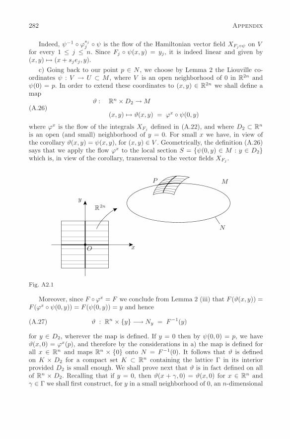
282 Appendix
Indeed, ψ−1 ϕsj
j ψ is the flow of the Hamiltonian vector field XFjψ on Vfor every 1 ≤ j ≤ n. Since Fj ψ(x, y) = yj , it is indeed linear and given by(x, y) → (x + sjej, y).
c) Going back to our point p ∈ N , we choose by Lemma 2 the Liouville co-ordinates ψ : V → U ⊂ M , where V is an open neighborhood of 0 in R
2n andψ(0) = p. In order to extend these coordinates to (x, y) ∈ R
2n we shall define amap
ϑ : Rn × D2 → M
(x, y) → ϑ(x, y) = ϕx ψ(0, y)(A.26)
where ϕx is the flow of the integrals XFjdefined in (A.22), and where D2 ⊂ R
n
is an open (and small) neighborhood of y = 0. For small x we have, in view ofthe corollary ϑ(x, y) = ψ(x, y), for (x, y) ∈ V . Geometrically, the definition (A.26)says that we apply the flow ϕx to the local section S = ψ(0, y) ∈ M : y ∈ D2which is, in view of the corollary, transversal to the vector fields XFj
.
y
R2n
O x
P M
N
Fig. A2.1
Moreover, since F ϕx = F we conclude from Lemma 2 (iii) that F (ϑ(x, y)) =F (ϕx ψ(0, y)) = F (ψ(0, y)) = y and hence
ϑ : Rn × y −→ Ny = F−1(y)(A.27)
for y ∈ D2, wherever the map is defined. If y = 0 then by ψ(0, 0) = p, we haveϑ(x, 0) = ϕx(p), and therefore by the considerations in a) the map is defined forall x ∈ R
n and maps Rn × 0 onto N = F−1(0). It follows that ϑ is defined
on K × D2 for a compact set K ⊂ Rn containing the lattice Γ in its interior
provided D2 is small enough. We shall prove next that ϑ is in fact defined on allof R
n × D2. Recalling that if y = 0, then ϑ(x + γ, 0) = ϑ(x, 0) for x ∈ Rn and
γ ∈ Γ we shall first construct, for y in a small neighborhood of 0, an n-dimensional
A.2 Action-angle coordinates, the Theorem of Arnold and Jost 283
lattice Γ(y) ⊂ Rn close to Γ(0) = Γ such that ϑ(x + γ(y), y) = ϑ(x, y) for every
γ(y) ∈ Γ(y).Let γ = γj ∈ Γ be an arbitrary basis vector of the lattice defined in (A.24).
Then ϕγ(p) = p and p = ψ(0). Hence, in the Liouville coordinates V ⊂ R2n
ψ−1 ϕγ ψ : (x, y) → (ξ, η)(A.28)
defines a symplectic diffeomorphism locally near the fixed point 0 in V .
Lemma 3. The symplectic map (A.28) in V is of the form
ξ = x − v(y) , v(y) = ∂∂yQ(y),
η = y(A.29)
for a smooth scalar function Q satisfying Q(0) = 0. Moreover, v(0) = 0.
Proof. Since, by definition, ϕγ ψ(x, y) = ψ(ξ, η) we conclude from F ϕx = F ,in view of Lemma 2 (ii), that
y = F ψ(x, η) = F ϕγ ψ(x, η) = F ψ(ξ, η) = η .
Every symplectic map extending the relation η = y is necessarily of the announcedform as we have seen in the previous section. That v(0) = 0 follows from ψ−1 ϕγ ψ(0) = 0.
By definition (A.28), ϕγ ψ(x, y) = ψ(ξ, η) and we conclude from Lemma 3and Lemma 2 that
ψ(x, y) = ϕγ+v(y) ψ(x, y)(A.30)
for (x, y) ∈ V ′ ⊂ V . We can do this for every basis vector γj ∈ Γ and findvj(y) = ∂
∂yQj(y) such that (A.30) holds true for γj +vj(y) replacing γ +v(y). We,
therefore, introduce the lattice Γ(y) ⊂ Rn by
Γ(y) =
γ(y) =n∑
j=1
njγj(y)∣∣∣ nj ∈ Z
(A.31)
where, in view of Lemma 3,
γj(y) = γj + vj(y) =∂
∂yWj(y) , 1 ≤ j ≤ n .
Here γj ∈ Γ and Wj are scalar functions satisfying Wj(0) = 0. Moreover, sincevj(0) = 0 we have γj(0) = γj and hence
Γ(0) = Γ .(A.32)
Consequently, for small y, the lattice vectors γj(y) are linearly independent andsatisfy, in view of (A.30)
ψ(x, y) = ϕγj(y) ψ(x, y) , 1 ≤ j ≤ n ,(A.33)
if (x, y) ∈ V ′ ⊂ V .
284 Appendix
Lemma 4. The map ϑ : (Rn × D2, ω0) → (M,ω) defined in (A.26) exists for all(x, y) ∈ R
n × D2 and satisfies
(i) ϑ∗ω = ω0 .
(ii) ϑ(x + γ(y), y
)= ϑ(x, y) , if γ(y) ∈ Γ(y) .
Proof. The map ϑ exists for (x, y) ∈ K×D2 with a compact set K ⊂ Rn containing
Γ(0) in its interior, if D2 is small enough. Since, for x small, we have, in view of(A.33),
ϑ(x + γj(y), y
)= ϕx+γj(y) ψ(0, y)
= ϕx ϕγj(y) ψ(0, y)
= ϕx ψ(0, y) = ϑ(x, y)
for every γj(y) ∈ Γ(y), the flow x → ϕxψ(0, y) does indeed exist for all x ∈ Rn by
the standard continuation theorem of solutions of ordinary differential equations.It remains to prove (i). If (x, y) ∈ R
n × D2 we choose x0 close to x such that(x − x0, y) ∈ V and represent the map ϑ in the form
ϑ(x, y) = ϕx0+(x−x0) ψ(0, y)
= ϕx0 ψ(x − x0, y) = ϕx0 ψ σx0(x, y)
where σx0(x, y) = (x − x0, y) and where we have used the corollary to Lemma 2.Hence, ϑ being locally a composition of symplectic mappings is indeed symplecticand the lemma is proved.
Recall that ϑ(Rn × y) ⊂ F−1(y). We claim that, for every y ∈ D2, the mapϑ induces a diffeomorphism
ϑ0 : Rn/Γ(y) −→ F−1(y)(A.34)
onto its image in F−1(y), which then is a torus Tn. We only have to prove thatϑ0 is injective provided y is sufficiently small. Arguing by contradiction there aresequences (xj , yj) and (x′
j , yj) satisfying
ϑ(xj , yj) = ϑ(x′j , yj) , yj → 0
xj − x′j /∈ Γ(yj) .
(A.35)
Taking a subsequence we may assume xj → x∗ and x′j → x′∗. Hence ϑ(x∗, 0) =
ϑ(x′∗, 0) and, therefore x∗ − x′∗ ∈ Γ(0) = Γ. Consequently, xj − x′j is close to a
point in Γ(yj). Since Γ(y) is discrete with distances between points greater than apositive constant uniformly in y, we conclude that xj−x′
j ∈ Γ(yj). This contradicts(A.35) and hence proves the claim (A.34).
A.2 Action-angle coordinates, the Theorem of Arnold and Jost 285
d) Finally, we normalize the lattices Γ(y) by means of another symplectic dif-feomorphism
σ : Rn × D1 → R
n × D2
(ξ, η) → (x, y) .
Recalling the definition of the lattice Γ(y) ⊂ Rn in (A.31) the symplectic map σ
is implicitly defined by the generating function
V (ξ, y) =n∑
j=1
ξjWj(y) ;(A.36)
hence,ηj = ∂
∂ξjV (ξ, y) = Wj(y)
xj = ∂∂yj
V (ξ, y) =n∑
s=1
ξs∂
∂yjWs(y) .
(A.37)
The first relation η = W (y) in (A.37) defines a local diffeomorphism near the fixedpoint y = 0. In the statement of Theorem 2 it is denoted by µ : D2 → D1. Thisfollows since
∂
∂yW (y) =
(γ1(y), . . . , γn(y)
)
is of rank n. Indeed the column vectors γj(y) are the n linearly independent gen-erators of Γ(y). Hence det(Vξ) = 0. Moreover, σ(ej , η) = (γj(y), y) for η = µ(y)and therefore
σ : Zn × η −→ Γ(y) × y , η = µ(y) .
The composition
Φ : = ϑ σ : (Rn × D1, ω0) −→ (M,ω)
is a symplectic map satisfying Φ(ξ + ej , η) = Φ(ξ, η). It induces a symplecticdiffeomorphism
Φ : Rn/Z
n × D1 −→ U ⊂ M
which is the desired map defining the action and angle variables denoted by (ξ, η) ∈Tn×D1. Indeed, using the definitions we compute µF Φ(ξ, η) = µF ϑσ(ξ, η) =µ F ϑ(x, y) = µ(y) = η as claimed in Theorem 2 whose proof is thereforecompleted.
The symplectic manifold (M,ω) is not required to be exact (exact meaning thatω = dϑ for a one-form ϑ on M). But it follows from the theorem that the restrictionof ω onto the image U = ψ(Tn×D) in M of the action-angle coordinates is an exactform. Indeed ω|U = dσ for the one-form σ = (ψ−1)∗λ, where λ =
∑nj=1 yjdxj on
Tn × D satisfies dλ = ω0. This allows us to obtain the action variables y = µ Fas “action integrals” of σ over closed curves on Nc ∩ U whose homology classesform a basis in H1(Nc ∩ U, Z) with µ(x) = y. Hence the name action variables.
286 Appendix
The action-angle variables (x, y) we constructed are, of course, not unique. Given aunimodular matrix M ∈ GL(n, Z), a function w(y) and constants c ∈ R
n, we findother action-angle variables (x′, y′) by means of the symplectic diffeomorphism ofTn × D:
x′ = M(x + ∂w
∂y (y))
y′ = (MT )−1y + c .
This corresponds to a change of the basis of the fundamental group of Tn by thematrix M and a phase shift ∂w
∂y (y) of the action variables. Straight lines on Tn aremapped into straight lines under this map.
We have constructed the action-angle coordinates near a torus and one canask how these local action-angle charts fit together. We do not discuss this globalquestion and refer instead to N. Nekhoroshev [168] (1972), to A.S. Mishchenko andA.T. Fomenko [158] (1978) and, in particular, to J.J. Duistermaat [64] (1980). In-tegrable systems constitute a very restricted even exceptional class of Hamiltoniansystems. Examples are described in the Notes [167], from which this appendix istaken with minor modifications. For interesting developments in the field of inte-grable systems we refer to J. Moser [166].
A.3 Embeddings of H1/2(S1) and smoothness of the action
In our proof of the smoothness of the action functional below the following em-bedding properties of the space H1/2(S1) introduced in Chapter 3 will be crucial.Formally they follow from Sobolev’s embedding theorem. However, for fractionalderivatives a separate proof is needed.
Theorem 3. If u ∈ H1/2(S1) then u ∈ Lp(S1) for every 1 ≤ p < ∞ and there areconstants Cp with
||u||Lp(S1) ≤ Cp||u||H1/2(S1) , u ∈ H1/2(S1) .
The embeddings are, moreover, compact.
Proof. It clearly suffices to find constants Cp satisfying the estimates for smoothfunctions u ∈ C∞(S1) only, since they are dense in H1/2(S1). Assuming for sim-plicity also the functions to have mean value zero we represent them as
u(e2πiϑ) =∑j∈Z
cj e2πiϑj with c0 = 0 and c−j = cj .
By definition,||u||2H1/2(S1) = 2π
∑j∈Z
|j| |cj |2 .
A.3 Embeddings of H1/2(S1) and smoothness of the action 287
Set z = re2πiϑ ∈ C. Considering S1 = ∂D as the boundary of the disc D = z ∈C : |z| ≤ 1 we can extend the function u to the harmonic function u(z) on D bysetting
u(z) =∑j =0
cjr|j|e2πiϑj =
12
(f(z) + f(z)
)
where
f(z) = 2∞∑
j=1
cj zj .
Since u(e2πiϑ) is in H1/2(S1) the function f is holomorphic in D and u(z) attainsthe desired boundary values. We claim
∫
D
|∇u|2 dx dy = ||u||2H1/2(∂D) .
Indeed using f ′(z) = ∂u∂x − i∂u
∂y and integrating over the angle variables first, wefind ∫
D
|∇u|2dx dy =∫D
|f ′(z)|2rdr dϑ
= 8π∞∑
j=1
j2|cj |21∫0
r2j−1dr = 8π∑j≥1
|cj |2 j2
2j
= 2π∑j∈Z
|j| |cj |2 = ||u||2H1/2(S1)
as claimed. A similar computation shows that ||u||L2(D) ≤ ||∇u||L2(D) using theassumption c0 = 0. The desired estimate of Theorem 3 is now an immediateconsequence of
Proposition 3. For 2 ≤ p < ∞ there are constants Cp, such that
||u||Lp(∂D) ≤ Cp
(||u||L2(D) + ||∇u||L2(D)
).
for u ∈ C1(D)
In order to prove this statement, which is a special case of a general ”trace”theorem, we start with a lemma.
Lemma 5. For 2 ≤ p < ∞ there are constants Cp satisfying
||u||Lp(∂D) ≤ Cp
(||u||L2p−2(D) + ||∇u||L2(D)
)
for u ∈ C1(D).
288 Appendix
Proof. Consider at first the function u = u(r, ϑ) on the annulus A = z|1/2 ≤|z| ≤ 1. By continuity of u we can find a radius 1
2< ρ < 1 with
||u||L1(A) =
1∫12
2π∫
0
|u(r, ϑ)|r dr dϑ =ρ
2
2π∫
0
|u(ρ, ϑ)|dϑ ≥ 14
2π∫
0
|u(ρ, ϑ)|dϑ .
Hence integrating
u(1, ϑ) = u(ρ, ϑ) +∫ 1
ρ
∂u
∂r(r, ϑ)dr
over the angle variable, we get
14||u||L1(∂D) ≤ ||u||L1(A) +
∣∣∣∣∣∣∂u
∂r
∣∣∣∣∣∣L1(A)
.
Replacing u by v = |u|p−1u, with p ≥ 2, using ∂v∂r
= p|u|p−1 ∂u∂r
and the Cauchy-Schwarz inequality we find
||u||Lp(∂D) ≤ Cp
(||u||Lp(A) + ||u||
p−1p
L2p−2(A)||∂u
∂r||
1p
L2(A)
),
with a constant Cp depending on p only. Using Young’s inequality (ab ≤ ap
p + bq
q
if 1p + 1
q = 1), we conclude
||u||Lp(∂D) ≤ Cp
(||u||L2p−2(A) + ||∂u
∂r||L2(A)
),
from which the lemma follows. In view of this lemma, Proposition 3 is a consequence of the next proposition
which is a special case of a more general Sobolev embedding theorem. It statesthat H1,2(D) is continuously embedded in Lp(D), for every p < ∞.
Proposition 4. There are constants Cp, 2 ≤ p < ∞ such that
||u||Lp(D) ≤ Cp
(||u||L2(D) + ||∇u||L2(D)
)
for all u ∈ C1(D).
Proof. First extend the functions u ∈ C1(D) to C1-functions of compact supportin a neighborhood of D. This may be achieved as follows. Choose χ ∈ C∞
c (R2)such that χ = 1 on D and χ = 0 outside a disc of radius 5
4 . Then define theextension of u = u(r, ϑ) by
u(1 + r, ϑ) = 4u(1 − 12r, ϑ) − 3u(1 − r, ϑ) · χ(1 + r, ϑ) .
A.3 Embeddings of H1/2(S1) and smoothness of the action 289
This defines a linear extension map E : C1(D) → C1c (Q) which is bounded in the
W 1,2 norm, where Q is a bigger domain. In order to prove the proposition it is,therefore, sufficient to find constants Cp such that for all u ∈ C1
c (Q)
||u||Lp(Q) ≤ Cp
(||u||L2(Q) + ||∇u||L2(Q)
).(A.38)
If u ∈ C1c (Q), then
|u(x, y)| =∣∣∣
x∫
−∞
∂u
∂x(t, y)dt
∣∣∣ ≤∞∫
−∞
∣∣∣∂u
∂x(t, y)
∣∣∣dt ,
and hence, with a similar estimate for the y-derivative:
|u(x, y)|2 ≤∞∫
−∞
∣∣∣∂u
∂x(t, y)
∣∣∣dt ·∞∫
−∞
∣∣∣∂u
∂y(x, t)
∣∣∣dt .
By integration, ∥∥∥u∥∥∥2
L2(Q)≤
∥∥∥∂u
∂x
∥∥∥L1(Q)
·∥∥∥∂u
∂y
∥∥∥L1(Q)
.
Replacing u by v = |u|t−1u, with t ≥ 2, we find by the Cauchy-Schwarz inequality
||u||2tL2t(Q) ≤ Ct||u||2t−2
L2t−2(Q) ||∂u∂x ||L2(Q)||∂u
∂y ||L2(Q)
≤ Ct||u||2t−2L2t−2(Q) ||∇u||2L2(Q) .
Hence by Young’s inequality,
||u||L2t(Q) ≤ Ct
(||u||L2t−2(Q) + ||∇u||L2(Q)
).(A.39)
If t = 2, we have the W 1,2 norm on the right hand side and hence by iterating theinequality (A.39) the desired estimate (A.38) follows for every 2 ≤ p < ∞. Thiscompletes the proof of Proposition 4 and the first claim of Theorem 3.
Finally we shall show that the embeddings H1/2 → Lp are compact for p < ∞.For the special case p = 2, this is proved in Chapter 3. Applying the Cauchy-Schwarz inequality to |u| |u|q−1 = |u|q , we find the following interpolation in-equality
||u||Lq ≤ ||u||1q
L2 ||u||1−1q
L2q−2 , q > 2 .
Since H1/2 → L2q−2 is continuous by the first part of Theorem 3 and H1/2 → L2 iscompact, we conclude from the above interpolation inequality that also H1/2 → Lq
is compact. This proves the second statement of Theorem 3.
290 Appendix
The case p = ∞ is excluded in Theorem 3 and we give an example of anunbounded function in H1/2(S1). If 0 < ε < 1
2then the function
u(eiϑ) : = Re[log(1 − eiϑ)]12−ε
belongs to H1/2(S1), where the branch of log is chosen so that log 1 = 0. In orderto verify this it suffices, to prove for f(z) := [log(1 − z)]
12−ε, that the integral∫
|z|<1
|f ′(z)|2 dx dy
is finite. We would like to add that a function u ∈ H1/2 not only belongs to Lp forevery 1 ≤ p < ∞ but even eαu2
is in L1 for every α ∈ R, and there is a constantC > 0 such that
2π∫0
e[u(eiϑ)]2 dϑ ≤ C for every u ∈ H1/2(S1) satisfying
||u||H1/2(S1) ≤ 1 and2π∫0
u(eiϑ)dϑ = 0 .
This result, due to D.E. Marshall, sharpens an estimate of A. Beurling and werefer to S.Y. Chang [40] and more recently W. Beckner [17].
Next we consider a smooth Hamiltonian H ∈ C∞(R×R2n , R) which is periodic
in time, H(t, x) = H(t + 1, x) for all (t, x) ∈ R × R2n. We assume that all the
derivatives of H have polynomial growth.
Theorem 4. The action a : H1/2(S1) → R, defined by
a(x) : =
1∫
0
H(t, x(t)
)dt ,
belongs to C∞(H1/2(S1), R).
Proof. Fixing an integer k we start with the Taylor formula for the function x →H(t, x):
H(t, y + η) =k∑
j=0
1j!
hj(t, y) · ηj + ok(η) ,
wherehj(t, y) · ηj : =
∑|α|=j
j!α!
DαxH(t, y)ηα
and y, η ∈ R2n. If x, ξ ∈ H1/2 we insert y = x(t) and η = ξ(t) and integrating over
t we find the Taylor formula for a in the form
a(x + ξ) =k∑
j=0
1j!
aj(x) · ξj + rk(x, ξ) ,
A.4 The Cauchy-Riemann operator on the sphere 291
with
aj(x) · ξj : =
1∫
0
hj
(t, x(t)
)· ξ(t)j dt .
Now aj(x) is a continuous j-linear form on H1/2 which, in addition, depends con-tinuously on x ∈ H1/2. This follows immediately from Holder’s inequality appliedto the above integral, using Theorem 3 and the assumption that the derivatives ofH are polynomially bounded. Moreover |rk(x, ξ)| ≤ Ck ·|ξ|k+1
1/2 . Since this holds truefor every k we conclude by the converse to Taylor’s theorem (see e.g R. Abrahamand J. Robbin [2]) that a is smooth and, as formally expected, has the derivatives
Dja(x) = aj(x)
for j ≥ 1. The proof of Theorem 4 is finished.
A.4 The Cauchy-Riemann operator on the sphere
The Cauchy-Riemann operator is the linear operator defined by
∂ : C∞(C, Cn) → C∞(C, Cn) : u → us + iut.
We drop for convenience the factor 12 in the usual definition of ∂. Here s + it are
the coordinates on C. Our first goal is to solve the equation
∂u = g
for given g ∈ D, where D denotes the vector space of compactly supported Cn-
valued smooth functions on C. If ε > 0 and u ∈ D we define the function Aεu :C → C
n using the Green’s function of ∂ by
(Aεu)(z) = − 12π
∫
|ξ|≥ε
1ξu(z + ξ)ds dt ,
where ξ = s + it, s, t ∈ R. Since u has compact support there exists a constantM > 0 depending on u, such that for all z1, z2 ∈ C
|u(z1) − u(z2)| ≤ M |z1 − z2|.
Using polar coordinates (r, θ) we can estimate
|(Aεu)(z2) − (Aεu)(z1)| ≤ 12π
∫|ξ|≥ε
∣∣∣u(z2+ξ)−u(z1+ξ)ξ
∣∣∣ds dt
≤ 12π
R∫ε
2π∫0
M |z1 − z2|drdθ
≤ MR|z2 − z1| ,
292 Appendix
where R > diameter ( suppu) + max|z1|, |z2|. The estimate implies that Aεu ∈C0(C, Cn). Similarly one finds for ε1, ε2 > 0
|(Aε1u)(z) − (Aε2u)(z)| ≤ ‖u‖0 |ε2 − ε1| .
Here ‖.‖0 denotes the sup-norm. By the latter estimate the limit of Aεu for ε → 0exists uniformly and defines a continuous function Au : C → C
n.
If e ∈ C is a vector of unit length, h ∈ R \ 0 and u ∈ D we denote by dhuthe difference quotient associated to h and e:
(dhu)(z) =u(z + he) − u(z)
h.
It follows immediately from the definition of A that
Adh = dhA.
From the definition we deduce that for every compact K ⊂ R2n there is a constant
M = MK such that |Aεu(z)| ≤ M ||u||0 for all u ∈ D having supp(u) ⊂ K. There-fore, also |Au(z)| ≤ M ||u||0. Consequently, denoting by De the directional deriva-tive associated to the vector e, we find for fixed z, that |(dhAu)(z)− (ADeu)(z)| =|A(dhu − Deu)(z)| ≤ M ||dhu − Deu||0 → 0 as h → 0, where M depends only onsupp(u). Hence ADe = DeA and repeating the arguments
DαAu = ADαu .
We see that A defines a linear map from D into C∞, satisfying, in addition,
A ∂ = ∂ A .
In fact, even more is true and we claim that
∂ A = Id on D .
In order to prove this we define v(s, t) = u(z + ξ) for a fixed z ∈ C and ξ = s + it.We compute for ξ = 0
1ξ (∂v)ds ∧ dt = 1
ξ
[∂v∂s + i∂v
∂t
]ds ∧ dt
= 1ξ
[(∂v∂s
)ds +
(∂v∂t
)dt
]∧ (dt − ids)
= −iξ (dv) ∧ (ds + idt)
= d(v 1
ξ(ds + idt)
)(−i) ,
A.4 The Cauchy-Riemann operator on the sphere 293
where we have used that d( 1ξ ) = − 1
ξ2 (ds + idt). Because u has compact supportwe infer by Stokes’ theorem for large R
Aε∂u(z) = −12π
∫ε≤|ξ|≤R
1ξ (∂u)(z + ξ)ds dt
= i2π
∫ε≤|ξ|≤R
d(u(z + ξ)( 1
ξ (ds + idt)))
= 12πi
∫|ξ|=ε
u(z + ξ) 1ξ (ds + idt)
= 12πi
2π∫0
u(z + εeiθ) 1εe−iθ(iε)eiθdθ
= 12π
2π∫0
u(z + εeiθ)dθ .
The last expression tends to u(z) as ε → 0. Thus we have proved A∂ = Id andhence ∂ A = Id as claimed. Next we study the asymptotic behaviour of Au(z)as z → ∞.
Proposition 5.(Au)(z) → 0 as |z| → ∞ for u ∈ D .
Proof. We choose R > 0 be so large that supp(u) ⊂ BR(0) and first observe that
(Au)(z) = − limε→0
12π
∫|ξ|≥ε
u(z + ξ) 1ξds dt
= − limε→0
12π
∞∫ε
2π∫0
u(z + reiθ)e−iθdr dθ
= − 12π
∞∫0
2π∫0
u(z + reiθ)e−iθ dr dθ .
For |z| > R consider the function v(r, θ) := u(z + reiθ)e−iθ. Pick (r0, θ0) in such away that z = −r0e
iθ0 . Then the support of v lies in a cone with vertex at 0 havingan angle σ so that
R
r0= sin
(σ
2
).
Moreover if (r, θ) is in this sector then v(r, θ) = 0 if
r ∈ [0, r0 − R] ∪ [r0 + R, +∞) .
This is illustrated by the following Fig. A4.1.
As r0 = |z| → ∞ we see that σ → 0. More precisely for |z| large
0 ≤ σ ≤ 4R
|z| .
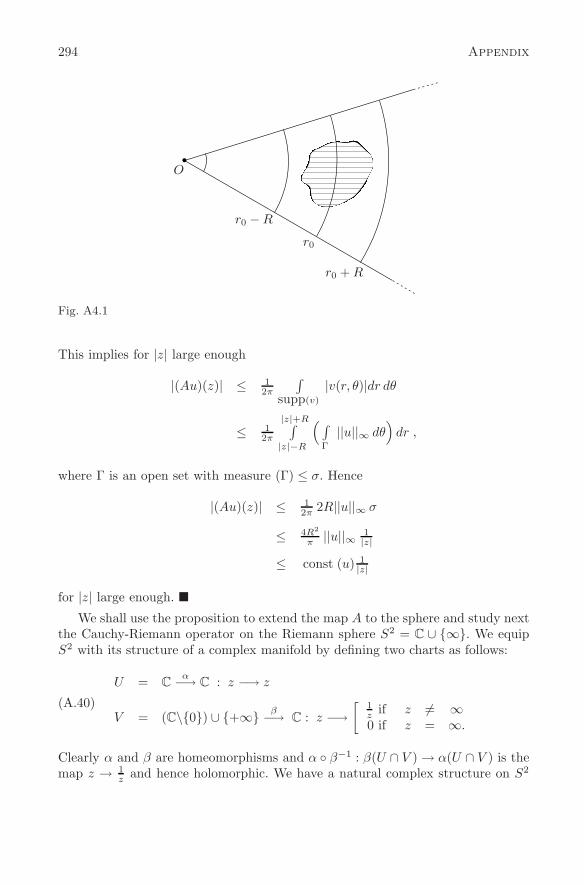
294 Appendix
O
r0 − R
r0
r0 + R
Fig. A4.1
This implies for |z| large enough
|(Au)(z)| ≤ 12π
∫supp(v)
|v(r, θ)|dr dθ
≤ 12π
|z|+R∫|z|−R
( ∫Γ
||u||∞ dθ)
dr ,
where Γ is an open set with measure (Γ) ≤ σ. Hence
|(Au)(z)| ≤ 12π 2R||u||∞ σ
≤ 4R2
π ||u||∞ 1|z|
≤ const (u) 1|z|
for |z| large enough. We shall use the proposition to extend the map A to the sphere and study next
the Cauchy-Riemann operator on the Riemann sphere S2 = C ∪ ∞. We equipS2 with its structure of a complex manifold by defining two charts as follows:
U = Cα−→ C : z −→ z
V = (C\0) ∪ +∞ β−→ C : z −→[
1z
if z = ∞0 if z = ∞.
(A.40)
Clearly α and β are homeomorphisms and α β−1 : β(U ∩ V ) → α(U ∩ V ) is themap z → 1
z and hence holomorphic. We have a natural complex structure on S2
A.4 The Cauchy-Riemann operator on the sphere 295
denoted by i. Consider now the vector bundles
S2 × Cn −→ S2
X −→ S2
where the fibre Xz over z ∈ S2 consists of all complex anti-linear maps φ : TzS2 →
Cn. In order to define the Cauchy-Riemann operator ∂ on the C∞-sections of these
bundles, we denote by C∞(S2×Cn) the space of smooth sections of S2×C
n → S2,i.e., C∞(S2 × C
n) = C∞(S2, Cn), and with C∞(X) the space of smooth sectionsof X → S2. We define ∂ : C∞(S2 × C
n) → C∞(X) by
(∂f)(z) = Tu(z) + i Tu(z)i ,(A.41)
where Tu(z) : TzS2 → C
n, z ∈ S2 is the tangent map of u. Note that
(∂u)(z) i = −i (∂u)(z) ,
so that ∂ is indeed well-defined.We now assume that g ∈ C∞(X). Using a partition of unity subordinate to
our distinguished atlas (A.40), we have the splitting
g = gU + gV ,
where supp(gU) ⊂ U , supp(gV ) ⊂ V . The map gU (z) : C → Cn is complex anti-
linear for every z ∈ U = C, and has compact support with respect to z. Hence
z → gU (z)(1)
belongs to D. We can solve
us + i ut = gU (·)(1) = : gU ∈ C∞(C, Cn)
for u ∈ C∞(C, Cn) byu = AgU .
We observe that
(∂u)(z)(1) =[(Tu)(z) + i Tu(z)i
](1)
= us(z) + i ut(z)
= gU (z)(1) .
Because ∂u(z) is anti-linear we have ∂u = gU over U = C. By Proposition 5, wehave u(z) → 0 as |z| → ∞ and, moreover, ∂u(z) = 0 outside the support of gU sothat u is holomorphic for |z| large. Consider the map on V \∞,
C\0 −→ Cn : z −→ u(
1z) = u β−1(z) .
296 Appendix
This map is holomorphic in a punctured neighborhood of 0 and u( 1z ) → 0 for
z → 0. Hence 0 is a removable singularity by the well-known classical result in thetheory of one complex variable. Therefore, u may be viewed as a smooth functionon S2 which vanishes at ∞. From Proposition 5 we conclude in particular
Proposition 6. The map A defines a linear operator from D into the subspacef ∈ C∞(S2, Cn)|f(∞) = 0 of C∞(S2, Cn), satisfying
∂ A = Id .
Back to our previous discussion, we have found u ∈ C∞(S2 × Cn) solving
the equation ∂u = gU and since S2\0 is biholomorphic to C, we find by thesame reasoning a gv ∈ C∞(S2 ×C
n) satisfying ∂v = gV . Therefore, it follows that∂(u+v) = gU +gV = g proving that ∂ is surjective. On the other hand, if ∂u = 0 weobtain a bounded holomorphic function u : C → C
n which by Liouville’s theoremis a constant map. Summing up we have proved
Theorem 5. The map ∂ : C∞(S2 × Cn) → C∞(X) is a surjective linear operator
whose kernel consists of all constant maps. As a real (respectively complex) linearoperator the kernel is of dimension 2n (respectively n).
Next we would like to study ∂ as an operator in a Sobolev space setting basedon Lp-spaces 1 < p < ∞. We start with the following estimate from Douglis andNirenberg, [63]. Denote by D1 the subspace of D consisting of all functions in Dwith support in the unit ball. We write | · |k,p for the norm defined by
|u|pk,p =∑|α|≤k
|Dαu|pLp(B1(0)) .
Here k ∈ N and 1 < p < ∞. The fundamental estimate given in [63] is the following
Theorem 6. For given k ∈ N and 1 < p < ∞ there exists a positive constantc = c(k, p) satisfying
|∂u|k,p ≥ c|u|k+1,p
for all u ∈ D1.In order to obtain some Sobolev type estimates for the section map ∂ : C∞(S2×
Cn) → C∞(X) we take a finite covering U1, . . . , Um of S2 so that Uj is biholomor-
phic to the open unit disc B around 0. Let β1, . . . , βn be a subordinate partitionof unity. Denoting by ϕj : Uj → B suitable biholomorphic diffeomorphisms wedefine a norm || ||k,p for k ∈ N, 1 < p < ∞, by
||u||pk,p =m∑
j=1
∣∣∣(βj ϕ−1j )(u ϕ−1
j )∣∣∣pk,p
.
It is easy to show that all the norms on C∞(S2×Cn) obtained by this procedure are
equivalent. For the bundle X → S2 we take smooth complex linear trivialisations
A.4 The Cauchy-Riemann operator on the sphere 297
ψj : X|Uj → B × Cn covering ϕj . This means that the following diagramm is
commutativeX |Uj
ψj−→ B × Cn
pr1
Ujϕj−→ B .
If f is a section of X we define the norm ||f ||k,p by
||f ||pk,p =m∑
j=1
∣∣∣ψj(ϕ−1j )
((βj ϕ−1
j )(f ϕ−1j )
)∣∣∣pk,p
.
Again all norms obtained this way are equivalent. Let us abbreviate ψj = ψj(ϕ−1j )
and βj = βj ϕ−1j . Then
ψj(z)(βj(z)(∂u)(ϕ−1
j (z)))
= βj(z)ψj(z)((Tu)(ϕ−1
j (z)) + i(Tu)(ϕ−1j (z))i
)
= βj(z)ψj(z)[(
T (u ϕ−1j )(z) + i(T (u ϕ−1
j )(z)i)Tϕj(z)
]
= βj(z)ψj(z)[(
T uj(z) + iT uj(z))i)Tϕj(z)
],
where uj = uj ϕ−1j . This gives immediately the estimate
∣∣∣ψj
(βj(∂u)(ϕ−1
j ))∣∣∣p
0,p≥ dp
j
∣∣∣βj
( ∂
∂s+ i
∂
∂t
)uj
∣∣∣p0,p
,
for a suitable constant dj independent of u. If d = infd1, . . . , dm, then
||∂u||0,p ≥ d
(m∑
j=1
∣∣∣βj
(∂∂s + i ∂
∂t
)uj
∣∣∣p0,p
)1/p
= d
(m∑
j=1
∣∣∣(
∂∂s + i ∂
∂t
)(βj uj) −
((∂∂s + i ∂
∂t
)βj
)uj
∣∣∣p0,p
)1/p
≥ d
(m∑
j=1
∣∣∣(
∂∂s + i ∂
∂t
)(βj uj)
∣∣∣p0,p
)1/p
− a
(m∑
j=1
∣∣∣χj uj
∣∣∣p0,p
)1/p
for a suitable constant a > 0 independent on the choice of u. Here χj is thecharacteristic function of the support of βj . Hence employing Theorem 6
||∂u||0,p ≥ d
(m∑
j=1
cp|βj uj |p1,p
)1/p
− a
(m∑
j=1
|χj uj |p0,p
)1/p
≥ c′||u||1,p − a′||u||0,p
for suitable constants a′, c′ > 0, independent of u. We have proved

298 Appendix
Theorem 7. There exist constants a, c > 0 such that for all u ∈ C∞(S2 × Cn)
||∂u||0,p ≥ c||u||1,p − a||u||0,p .
Define W 1,p(S2×Cn) and Lp(X) as the completions of the spaces C∞(S2×C
n)and C∞(X) with respect to the norms || ||1,p and || ||0,p. By the compact embeddingof W 1,p → Lp we find in view of Theorem 7 that ∂ : W 1,p(S2 ×C
n) → Lp(X) hasclosed range. Since in view of Theorem 5 the range contains the dense set C∞(X)we deduce ∂(W 1,p(S2 × C
n)) = Lp(X) and hence ∂ is surjective.On the other hand, by interior elliptic regularity theory or by the well-known
fact that a holomorphic distribution is a holomorphic function, we conclude from∂u = 0 that u is holomorphic and bounded and consequently constant.
We have proved
Theorem 8. The operator ∂ : W 1,p(S2 × Cn) → Lp(X) is a surjective Fredholm
operator whose kernel consists of the constant functions. Hence the index of ∂ asa real operator is 2n.
With some more efforts and rudimentary functional analysis one can prove
Theorem 9. For every k ∈ N and 1 < p < ∞ there are positive constants c = c(k, p)and a = a(k, p) such that
||∂u||k,p ≥ c||u||k+1,p − a||u||0,p ,
for all u ∈ C∞(S2 × Cn).
As an operator from W k+1,p(S2×Cn) to W k,p(X) the linear operator ∂ is again
a surjective Fredholm operator whose kernel consists of the constant functions. Fora general treatment of first order elliptic systems, we refer the reader to Vekua’sbook, [215], or its English translation.
A.5 Elliptic estimates near the boundary and an application
Denote by B+ε the half ball given by
B+ε = z ∈ C | |z| < ε,Re(z) ≥ 0
with boundary ∂B+ε = (−ε, ε)i.
Let || · ||k,p,Ω for k ∈ N, 1 < p < ∞ denote the usual Sobolev norms, i.e.,
||u||pk,p,Ω =∑|α|≤k
||Dαu||pLp(Ω) .
The classical estimate, which for example can be found in Vekua [215], for ∂ =∂∂s + i ∂
∂t is
A.5 Elliptic estimates near the boundary and an application 299
Theorem 10. Given ε > 0, k ∈ N, 1 < p < ∞, there exists a constant c = c(k, p, ε) >0 such
||∂u||k,p,B+ε
≥ c||u||k+1,p,B+ε
for all smooth u : B+ε → C
n with compact support in B+ε satisfying the boundary
conditionu(∂B+
ε ) ⊂ Rn .
Using this estimate and the usual differential quotient technique from standardelliptic regularity theory we obtain the following regularity result.
Let J be a smooth almost complex structure defined on Cn (or at least near
0) such that J(0) = i. Assume
u : B+ε → C
n
is of class W 1,p with p > 2 and satisfies
u(0) = 0
u((−ε, ε)i
)⊂ R
n
∂u∂s + J(u)∂u
∂t = 0 on B+ε
where B+ε = B+
ε \(−ε, ε)i. We have the following
Theorem 11. Under the above assumptions there exists δ ∈ (0, ε) such that u|B+δ
is smooth.Our next aim is to give an application to a regularity question raised in Chapter
6. Letw : [−ε, ε] × [−ε, ε] −→ C
n
be of class W 1,p, 2 < p < ∞. Assume w(0) = 0, and J is an almost complexstructure defined on a sufficiently large neighborhood of zero such that J(0) = i.Assume H : [−ε, ε] × U → C
n is a smooth map, where U is a sufficiently largeneighborhood of 0 in C
n. Moreover, let H ′(0, 0) = 0, where H ′ is the gradient withrespect to the second variable for some Riemannian metric on U .
We consider the partial differential equation
∂w
∂s+ J(w)
∂w
∂t+ χ[0,∞)(s)H ′(t, w) = 0(A.42)
on (−ε, ε)× (−ε, ε). Here χ[0,∞) is the characteristic function of [0,∞). The amaz-ing fact is that
w |([−δ, 0] × [−δ, δ]
)
andw |
([0, δ] × [−δ, δ]
)
300 Appendix
are smooth for some sufficiently small δ ∈ (0, ε). In particular,
w |(0 × [−δ, δ]
)−→ C
n
is smooth. Note that w|([−δ, δ] × [−δ, δ]) is not smooth since the derivatives inthe s-direction do not match. The above proof of the smoothness assertion will bereduced by a series of transformations to Theorem 11.
For simplicity of the argument we assume that all data H and J are defined onthe whole of C
n. Define an almost complex structure J on [0, ε]× [−ε, ε]×Cn ×C
n
by
J(s, t, u, v)(a, b, h, k) =(− b, a, J(u)h + bH ′(t, u) + aJ(u)H ′(t, u),−J(v)k
),
The definition of J is motivated by Gromov’s trick and something that one couldcall the “inverse reflection principle”. It will turn out that a solution w of (A.42)gives a holomorphic map α on [0, ε) × [−ε, ε) for the structure J .
We leave it to the reader to verify that J2 = −Id. Let
j = J(0, 0, 0, 0) .
We observe that
j(a, b, h, k) =(− b, a, ih + bH ′(0, 0) + aiH ′(0, 0),−ik
).
Define a linear real subspace of R × R × Cn × C
n by
T = (0, b, h, h, ) | b ∈ R, h ∈ Cn .
Clearly dimR(T ) = 2n + 1 =: N . We note that
T ∩ jT = 0 .(A.43)
Indeed, if
(0, b1, h1, h1) = j(0, b2, h2, h2)
=(− b2, 0, ih2 + b2 H ′(0, 0),−ih2
),
we find b1 = b2 = 0 implying
i h2 = h1
−i h2 = h1,
and, therefore, h1 = h2 = 0. Define a map α : [0, ε] × [−ε, ε] → R × R × Cn × C
n
byα(s, t) =
(s, t, u(s, t), u(−s, t)
).
A.5 Elliptic estimates near the boundary and an application 301
Thenα(0, t) =
(0, t, u(0, t), u(0, t)
)∈ T
for t ∈ [−ε, ε]. Moreover α is in W 1,p([0, ε]× [−ε, ε], R×R×Cn ×C
n), since u, byassumption, belongs to this space. On (0, ε) × (−ε, ε) we compute
αs(s, t) + J(α(s, t)
)(αt(s, t)
)
=(1, 0, us(s, t),−us(−s, t)
)
+(− 1, 0, J(u(s, t))ut(s, t) + H ′(t, u(s, t)),−J(u(−s, t)ut(−s, t)
)
= (0, 0, 0, 0) .
In view of (A.43) the set T is a totally real subspace of (R × R × Cn × C
n, j). Itis a simple exercise to find a complex linear map
Φ : (R × R × Cn × C
n, j) −→ (CN , i)
mapping T onto RN . Recall that N = 2n + 1. Define β = Φ α and an almost
complex structure J on CN by
J(A) = ΦJ(Φ−1(A)
)Φ−1 .
We find thatJ(0) = ΦjΦ−1
= iΦΦ−1
= i .
Moreover, on (0, ε) × (−ε, ε),
βs + J(β)βt
= Φαs + ΦJ(Φ−1Φα)Φ−1Φαt
= Φ[αs + J(α)αt]
= 0 .
Finally, we observe thatβ(0, t) ∈ R
N
for t ∈ (−ε, ε). Applying Theorem 11 we deduce, since β ∈ W 1,p([0, ε]×[−ε, ε], CN )and β(i(−ε, ε)) ⊂ R
N , that β is smooth on [0, δ]× [−δ, δ] for some δ ∈ (0, ε). Hence
[0, δ] × [−δ, δ] → Cn : (s, t) → u(s, t)
302 Appendix
and[0, δ] × [−δ, δ] → C
n : (s, t) → u(−s, t)
are smooth, as we wanted to prove.We conclude with an observation used in Chapter 6. Recall the definition of
ST in Chapter 6 and assume w : ST → M solves
0 = ∂w + χ[−T,T ]×S1
(H ′(t, w)dt − J(u)H ′(t, w)ds
).(A.44)
Taking suitable complex coordinates near a point (T0, t0), respectively, (−T0, t0)in ZT ⊂ ST and suitable symplectic coordinates near w(T0, t0), respectively,w(−T0, t0) in M , we see that (A.44) looks, in these coordinates, like (A.42). Wededuce, in particular, since T0 was arbitrary, that the loops t → w(−T, t) andt → w(T, t) are smooth.
A.6 The generalized similarity principle
Let D be the closed unit disk D = z ∈ C| |z| ≤ 1. We denote by A ∈L∞(D,LR(Cn)) a mapping which associates with z ∈ D a real linear map A(z) :C
n → Cn, so that the assignment z → A(z) is essentially bounded. Let z → J(z) be
a smooth map associating with z ∈ D a complex structure on Cn, i.e J(z)2 = −1,
and J(z) : Cn → C
n is a real linear map. We consider a solution w : D → Cn of
the first order elliptic system
∂w
∂s+ J(z)
∂w
∂t+ A(z)w = 0 and w(0) = 0 ,(A.45)
where z = s + it. We shall show that w is represented locally near 0 by a holo-morphic map. Define Dδ = z ∈ D| |z| ≤ δ. Generalizing a result of T. Carleman[37] to systems we shall prove
Theorem 12. There exist 0 < δ < 1, a holomorphic map σ : Dδ → Cn and a
continuous map Φ : Dδ → GlR(Cn),
Φ ∈⋂
2<p<∞W 1,p
(Dδ,GlR(Cn)
),
satisfying on Dδ,J(z)Φ(z) = Φ(z)i
andw(z) = Φ(z)σ(z) .
It follows, in particular, that if 0 is a cluster point of zeros of the solution w,then it is also a cluster point of zeros of the holomorphic map σ, implying σ ≡ 0and therefore w ≡ 0 on Dδ. This was used in the proof of the Arnold conjecture(Lemma 2 in 6.4).
A.6 The generalized similarity principle 303
Proof. Reducing the local statement to a global one, the theorem will be obtainedas a corollary of Theorem 8 in A.4. We shall view the disk D as a subset ofC ⊂ C ∪ ∞ = S2 and begin by rewriting equation (A.45). We choose a smoothmap z → Ψ(z) from D into GlR(Cn) satisfying J(z)Ψ(z) = Ψ(z)i. Then we definev : D → C
n byw(z) = Ψ(z)v(z) ,
and compute:
0 = ∂w∂s + J(z)∂w
∂t + A(z)w
= Ψ(
∂v∂s
+ i∂v∂t
)+ AΨv +
(∂Ψ∂s
+ J ∂Ψ∂t
)v
= Ψ[
∂v∂s + i∂v
∂t + Ψ−1AΨv + Ψ−1(
∂Ψ∂s + J ∂Ψ
∂t
)v]
= Ψ[
∂v∂s + i∂v
∂t + Bv]
.
We see that v solves on D the equation
∂v
∂s+ i
∂v
∂t+ B(z)v = 0 and v(0) = 0 ,(A.46)
where B ∈ L∞(D,LR(Cn)). Now we represent B(z) as follows:
B(z) = Bl(z) + Ba(z) ,
where Bl(z) is complex linear and Ba(z) complex anti-linear. We denote by Γ :C
n → Cn the anti-linear complex conjugation map h → h, and choose C ∈
L∞(D,LC(Cn)) in such a way that
C(z)v(z) = v(z) , z ∈ D
where v is the given solutions of (A.46). Define E ∈ L∞(D,LC(Cn)) by
E(z) = Bl(z) + Ba(z) Γ C(z) .
Then E(z) is complex linear and
E(z)v(z) = B(z)v(z) , z ∈ D .
Therefore v satisfies on D,
∂v
∂s+ i
∂v
∂t+ E(z)v = 0 and v(0) = 0 ,(A.47)
where now E ∈ L∞(D,LC(Cn)). Observe that LC(Cn) = L(Cn) ∼= Cn2
. With thenotations introduced in Appendix 4, we consider, for 1 < p < ∞, the Cauchy-Riemann operator between sections,
∂ : W 1,p(S2 × L(Cn)
)→ Lp(X) ,
304 Appendix
where the fibre Xz, z ∈ S2 of the vector bundle X → S2 is the vector space con-sisting of all complex anti-linear maps TzS
2 → L(Cn). By Theorem 8 in Appendix4, the mapping
G : W 1,p(S2 × L(Cn)
)→ Lp(X) × L(Cn)
G(Z) : =(∂Z, Z(0)
),
is a linear isomorphism if 2 < p < ∞. Note that in the case 2 < p < ∞ wecan estimate the C0-norm in terms of the W 1,p-norms on 2-dimensional domains(Sobolev embedding theorem). If G(Z) = (0, Id) we infer that Z(z) = Id forz ∈ S2. Hence if a linear map : W 1,p(S2 × L(Cn)) → Lp(X) is small (in theoperator norm) then the perturbed map G, defined by
G(Z) =(∂Z + (Z) , Z(0)
),
is still an isomorphism, and Z = G−1(0, Id) is a map S2 → Gl(Cn) satisfyingZ(0) = Id. If z ∈ S2 we define E(z) : L(Cn) → Xz as follows. If z ∈ D we set
E(z)(Z) = E(z) Zds − i E(z) Z dt ,
and if z ∈ S2\D we set E(z) = 0. Then
E(z) ∈ L(L(Cn), Xz
);
moreover, z → E(z) belongs to L∞. For 0 < ε < 1 we denote by χε the character-istic function of the closed disk Dε, and define ε ∈ L(W 1,p(S2 ×L(Cn)), Lp(X))by
(εZ)(z) : = χε(z)E(z) Z(z) .
By the Sobolev embedding theorem we can estimate, if 2 < p < ∞,
||εZ||0,p ≤ (πε2)1p ||E||L∞ ||Z||L∞
≤ c(ε)||Z||1,p ,
where c(ε) → 0 if ε → 0. Consider now the special perturbation Gε := Gεand
define Z∗ : S2 → L(Cn) by
Z∗ = G−1ε (0, Id) .(A.48)
If ε > 0 is sufficiently small, then Z∗(z) ∈ Gl(Cn) for all z ∈ S2, hence is invertible;moreover, Z∗(0) = Id. Finally we define σ : Dε → C
n by
v(z) = Z∗(z)σ(z) ,
A.7 The Brouwer degree 305
and compute, for z ∈ Dε,
0 = ∂v∂s + i∂v
∂t + E(z)v
=(
∂Z∗
∂s+ i∂Z∗
∂t+ EZ∗
)σ + Z∗
(∂σ∂s
+ i∂σ∂t
)
=[(
(∂ + E)Z∗)(z)(1)
]σ(z) + Z∗
(∂σ∂s + i∂σ
∂t
)
= Z∗(
∂σ∂s + i∂σ
∂t
).
Here 1 is the obvious tangent vector in TzS2 = TzC ∼= C at z ∈ Dε ⊂ S2.
Since Z∗(z) is invertible if z ∈ Dε, we conclude that the map σ : Dε → Cn
is holomorphic. Defining Φ(z) := Ψ(z)Z∗(z), for z ∈ Dε, we obtain, using thedefinitions, the required representation:
w(z) = Ψ(z)v(z)
= Ψ(z)Z∗(z)σ(z)
= Φ(z)σ(z) .
From w(0) = 0 we deduce σ(0) = 0. In addition,
Φ(z)i = Ψ(z)Z∗(z)i
= Ψ(z)iZ∗(z)
= J(z)Ψ(z)Z∗(z)
= J(z)Φ(z) ,
as desired.So far, however, the δ constructed does depend on the p chosen. In order to
find a δ independent of p we carry out the above procedure for a fixed p0 to find acorresponding δ0 > 0. Then we employ inner elliptic regularity theory in order toconclude that Z∗ belongs to W 1,p
loc (Bδ0 ,LR(C)) for every p. Now we can take anyδ < δ0 and the proof of Theorem 12 is complete.
Related results and applications to the transversality questions involved in theconstruction of Floer homology are contained in A. Floer, H. Hofer and D. Salamon[87].
A.7 The Brouwer degree
In the following we shall describe the so called Brouwer degree or mapping de-gree used in Chapter 2. It serves as a qualitative criterion for the solvability of anonlinear equation
f(x) = y
306 Appendix
for x. This degree is an integer which “algebraically counts” the number of solu-tions. To be more precise we consider open bounded sets U ⊂ R
n and continuousmaps f : U → R
n. Given y ∈ Rn, the triplet (f, U, y) is called admissible, if
y /∈ f(∂U). The aim is to associate with every admissible triplet an integer, de-noted by d(f, U, y) such that the assignment
(f, U, y) → d(f, U, y)
satisfies some natural properties formulated in the following axioms.
Axiom 1. (Solution property)Assume (f, U, y) is admissible. If d(f, U, y) = 0 then there exists a solution x ∈ Uof f(x) = y.
The equations f(x) = y and f(x) − y = 0 have the same solutions x, and wetherefore require
Axiom 2. (Naturality)If (f, U, y) is admissible, then
d(f, U, y) = d(f − y, U, 0).
Assume (f, U, y) is admissible and V ⊂ U is an open set containing all thesolutions, i.e, (f |U)−1(y) ⊂ V . Then (f, V, y) is also admissible and has the samesolutions, hence we postulate:
Axiom 3. (Excision)If (f, U, y) is admissible and if the open set V ⊂ U satisfies f−1(y) ⊂ V , then
d(f, U, y) = d(f, V, y).
We wish the degree to “count” the solutions and hence require an additivityproperty:
Axiom 4. (Additivity)Assume (f, U, y) and (f, V, y) are admissible and U ∩ V = ∅. Then (clearly (f, U ∪V, y) is admissible)
d(f, U ∪ V, y) = d(f, U, y) + d(f, V, y) .
The next axiom is the most important one and crucial for the applications. Wewant the solution criterion to be stable under perturbation and require that d isinvariant under continuous deformations:
Axiom 5. (Homotopy invariance)Let t → (ft, U, y), 0 ≤ t ≤ 1 be an admissible deformation, i.e, f : [0, 1] × U → R
n
is continuous and (ft, U, y) is admissible for every 0 ≤ t ≤ 1. Then
d(f0, U, y) = d(f1, U, y) .
Finally, we normalize using a simple model equation.
A.7 The Brouwer degree 307
Axiom 6. (Normalization)
d(Id,B1(0), 0
)= 1 ,
where B1(0) is the open unit ball centered at the origin 0 in Rn.
For the moment, let us assume that such a d, satisfying these axioms exists.We prove that the axioms uniquely determine d. It is called the Brouwer degreeor mapping degree.
Assume first, that U is open and 0 /∈ U . Then (Id, U, 0) is admissible. Sincethere is no solution of Id(x) = 0 in U we conclude that d(Id, U, 0) = 0 in view ofAxiom 1. Next we consider the linear map f = T ∈ Gl(Rn).
Lemma 6. Assume U is a bounded open neighborhood of 0 and T ∈ Gl(Rn). Then
d(T,U, 0) = sign det(T ) .
Proof. Recall that Gl(Rn) = G+ ∪ G− where G± = T ∈ Gl(Rn)| ± det(T ) > 0;G+ and G− are pathwise connected. Define ϑ±1 ∈ Gl(Rn) by
ϑ±1 = diag (±1, 1, . . . , 1) .
Then ϑ+ ∈ G+ and ϑ− ∈ G−. Put ε = sig det (T ) and choose a continuous patht → Tt in Gε connecting T0 = ϑε with T1 = T . Then t → (Tt, U, 0) is an admissibledeformation and we obtain by Axiom 5
d(ϑε, U, 0) = d(T,U, 0) .
Since 0 is the unique solution we find by applying the excision Axiom twice thatd(T,U, 0) = d(ϑε, U, 0) = d(ϑε, B1(0), 0). If ε = 1 we employ Axiom 6 to find
d(T,U, 0) = d(Id,B1(0), 0
)= 1
= sign det(T ) .
In order to deal with the case ε = −1, we define ϕτ : [−1, 1] → R by ϕτ (t) =|t| − 1
2 + τ , for all 0 ≤ τ ≤ 1 and introduce fτ : [−1, 1] × Bn−11 (0) → R
n by
fτ (x1, . . . , xn) =(ϕτ (x1), x2, . . . , xn
).
Then (fτ , (−1, 1) × Bn−11 (0), 0) is an admissible homotopy. If τ = 1 the equation
f1(x) = 0
has no solutions in the associated open set. Hence by Axiom 5
d(fτ , (−1, 1) × Bn−1, 0
)= 0 ,
308 Appendix
for every τ ∈ [0, 1]. If τ = 0, then the equations |x1| − 12 = 0, xj = 0 for 2 ≤ j ≤ n,
have precisely the two solutions
x− = (−12, 0, 0, · · · , 0), x+ = (
12, 0, . . . , 0)
where x− ∈ V− := (− 34,− 1
4)×Bn−1 and x+ ∈ V+ := ( 1
4, 3
4)×Bn−1. Consequently,
by excision and additivity we obtain
0 = d(f0, V−, 0) + d(f0, V+, 0) .
For x ∈ V− we have f0(x) = (−x1 − 12 , x2, . . . , xn) and for x ∈ V+ we have
f0(x) = (x1 − 12, x2, . . . , xn), hence the previous equation is written
0 = d(ϑ− − x+, V−, 0) + d(ϑ+ − x+, V+, 0) ,
and by excision,
0 = d(ϑ− − x+, Bn, 0) + d(ϑ+ − x+, Bn, 0) .
Using the homotopy invariance we can get rid of the term x− to obtain
0 = d(ϑ−, Bn, 0) + d(ϑ+, Bn, 0)
= d(ϑ−, Bn, 0) + 1 .
We deduce, that also for ε = −1,
d(T,U, 0) = d(ϑ−, Bn, 0) = −1
= sign det(T ) ,
and the proof of Lemma 6 is complete. Assume now that (f,Bε(x0), 0) is admissible for some ε > 0. Assume, in addi-
tion that f is differentiable and satisfies
f−1(0) = x0 and f ′(x0) ∈ Gl(Rn) .
Lemma 7.d(f,Bε(x0), 0
)= sign det
(f ′(x0)
).
Proof. Define ft(x) := tf(x)+ (1− t)f ′(x0)(x−x0). Since f ′(x0) ∈ Gl(Rn) we finda small 0 < δ ≤ ε such that ft(x) = 0 if |x| = δ, for all 0 ≤ t ≤ 1. Using excisionand homotopy invariance we conclude that
d(f,Bε(x0), 0
)= d
(f,Bδ(x0), 0
)
= d(f ′(x0)(x − x0), Bδ(x0), 0
)
= d(f ′(x0)(x − x0), BR(0), 0
),
A.7 The Brouwer degree 309
where R > 0 is so large, that Bδ(x0) ⊂ BR(0). Choosing R large enough we nowget rid of the term −f ′(x0)x0 through an admissible homotopy and obtain
d(f,Bε(x0), 0
)= d
(f ′(x0), BR(0), 0
).
But by excision the right hand side does not depend on the size of R; in view ofLemma 6, the proof of Lemma 7 is therefore complete.
Now we appeal to two classical results in differential topology.
Lemma 8. Let Ω ⊂ Rn be a bounded open domain and f : Ω → R
n a continuousmap. Given ε > 0 there exists a smooth map g : Ω → R
n satisfying
|f(x) − g(x)| < ε for x ∈ Ω .
Proof. In view of the classical Stone-Weierstrass theorem we can take for g apolynomial approximation of f .
The second result we need is a version of the Morse-Sard theorem. Recall thaty ∈ R
n is a regular value for f if f ′(x) ∈ Gl(Rn) for all x ∈ f−1(y).
Lemma 9. Let U ⊂ Rn be open and f : U → R
n a smooth map. Then the set ofregular values for f is residual in R
n and therefore dense.A proof can be found in the book on differential topology by M. Hirsch [113].If (f, U, y) is an admissible pair we define
σ : = infx∈∂U
|f(x) − y| ,
then σ > 0, and by Lemma 8 we can pick g smooth with |f(x) − g(x)| < εon U , where ε < σ/2. Then ft = (1 − t)f + tg defines an admissible homotopyt → (ft, U, y). Hence by Axiom 5 and Axiom 2
d(f, U, y) = d(g, U, y) = d(g − y, U, 0) .
For every z ∈ Bε(y) the homotopy t → gt := g− y + tz is admissible for (U, 0) andhence
d(f, U, y) = d(g − z, U, 0) ,
for every z ∈ Bε(y). In view of Lemma 4 we can pick z0 ∈ Bε(y) which is a regularvalue of g. Hence
d(f, U, y) = d(g, U, z0) .
Since U is compact and z0 regular, the set g−1 = x1, x2, . . . , xk is finite. Byexcision and additivity we, therefore, find for τ > 0 sufficiently small, that
d(f, U, y) =k∑
j=1
d(g,Bτ (xj), z0
)
=k∑
j=1
d(g − z0, Bτ (xj), 0
)
=k∑
j=1
sign det(g′(xj)
),
310 Appendix
where we have used Lemma 7. Summarizing, under the assumption that a degreed satisfying the Axioms 1-6 exists we conclude
Proposition 7.
(i) Assume (f, U, y) is admissible, f is smooth and y a regular value. Then
d(f, U, y) =∑
x∈f−1(y)
sign det(f ′(x)
).
(ii) If (f, U, y) is admissible, then there exists an admissible (g, U, y) homotopicto (f, U, y), where g is smooth and y is a regular value for g. In particular,
d(f, U, y) =∑
x∈g−1(y)
sign det(g′(x)
).
Proposition 7 shows that the degree d is uniquely determined by the Axioms1-6, and we shall establish its existence. The usual approach is to start with theformula (i) as the definition of d(f, U, y) if f is smooth with regular value y. Thedegree d(f, U, y) of a general admissible triplet is then defined as d(g, U, y) for asmooth g close to f having the regular value y. Then one verifies the axioms. Thecrucial step is to verify at first that this definition is independent of the choiceof the approximation g. The argument is as follows. If g0 and g1 are two smoothapproximations of f one defines the admissible deformation G : [0, 1] × U → R
n
by G(t, x) = (1 − t)g0(x) + tg1(x). One can assume y to be a regular value for allthree maps g1, g2 and G. Since G is admissible, G−1(y) ⊂ [0, 1] × U , and since yis a regular value of G, the solution set G(t, x) = y is either empty or consists offinitely many disjoint, compact, connected 1-dimensional manifolds. According tothe classification of 1-dimensional manifolds, see J. Milnor [157], each componentis either a circle (if it has no boundary) or a closed interval in which case its twoboundaries belong to the faces 0 × U, 1 × U as illustrated in the followingfigure:
0 × U 1 × U
x1
x2
xm
ξ1
ξ2
ξk
S1
Fig. A7.1
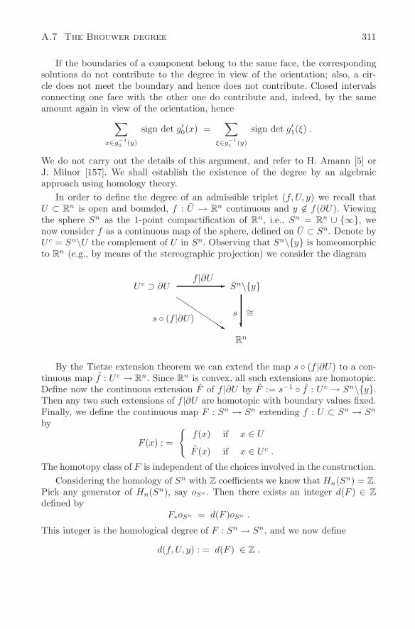
A.7 The Brouwer degree 311
If the boundaries of a component belong to the same face, the correspondingsolutions do not contribute to the degree in view of the orientation; also, a cir-cle does not meet the boundary and hence does not contribute. Closed intervalsconnecting one face with the other one do contribute and, indeed, by the sameamount again in view of the orientation, hence
∑x∈g−1
0 (y)
sign det g′0(x) =∑
ξ∈g−11 (y)
sign det g′1(ξ) .
We do not carry out the details of this argument, and refer to H. Amann [5] orJ. Milnor [157]. We shall establish the existence of the degree by an algebraicapproach using homology theory.
In order to define the degree of an admissible triplet (f, U, y) we recall thatU ⊂ R
n is open and bounded, f : U → Rn continuous and y ∈ f(∂U). Viewing
the sphere Sn as the 1-point compactification of Rn, i.e., Sn = R
n ∪ ∞, wenow consider f as a continuous map of the sphere, defined on U ⊂ Sn. Denote byU c = Sn\U the complement of U in Sn. Observing that Sn\y is homeomorphicto R
n (e.g., by means of the stereographic projection) we consider the diagram
U c ⊃ ∂Uf |∂U
Sn\y
∼=s
Rn
s (f |∂U)
By the Tietze extension theorem we can extend the map s (f |∂U) to a con-tinuous map f : U c → R
n. Since Rn is convex, all such extensions are homotopic.
Define now the continuous extension F of f |∂U by F := s−1 f : U c → Sn\y.Then any two such extensions of f |∂U are homotopic with boundary values fixed.Finally, we define the continuous map F : Sn → Sn extending f : U ⊂ Sn → Sn
by
F (x) : =
f(x) if x ∈ U
F (x) if x ∈ U c .
The homotopy class of F is independent of the choices involved in the construction.Considering the homology of Sn with Z coefficients we know that Hn(Sn) = Z.
Pick any generator of Hn(Sn), say oSn . Then there exists an integer d(F ) ∈ Z
defined byF∗oSn = d(F )oSn .
This integer is the homological degree of F : Sn → Sn, and we now define
d(f, U, y) : = d(F ) ∈ Z .
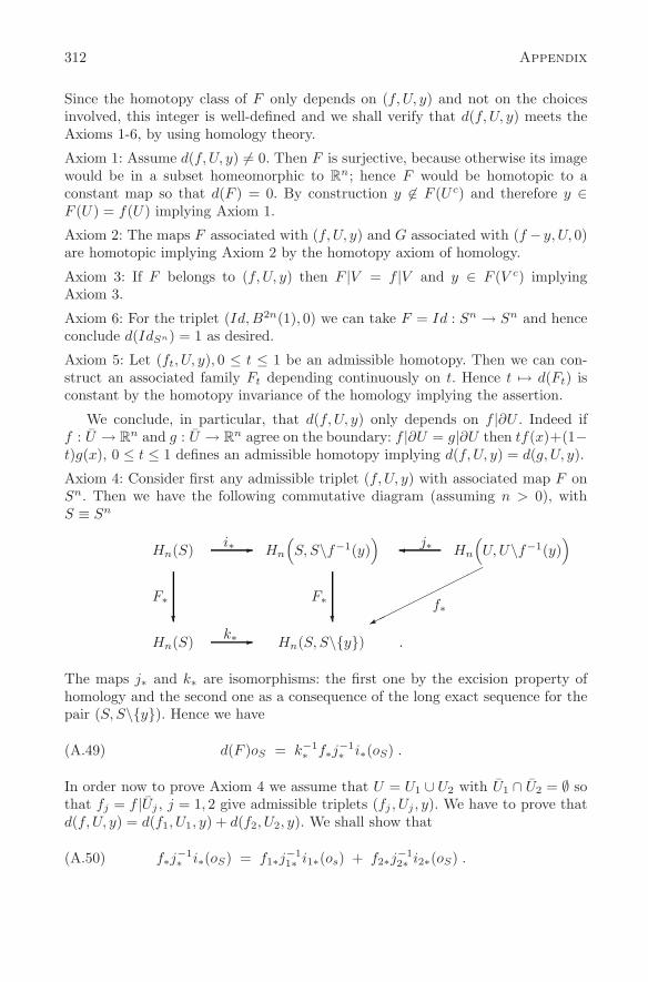
312 Appendix
Since the homotopy class of F only depends on (f, U, y) and not on the choicesinvolved, this integer is well-defined and we shall verify that d(f, U, y) meets theAxioms 1-6, by using homology theory.
Axiom 1: Assume d(f, U, y) = 0. Then F is surjective, because otherwise its imagewould be in a subset homeomorphic to R
n; hence F would be homotopic to aconstant map so that d(F ) = 0. By construction y ∈ F (U c) and therefore y ∈F (U) = f(U) implying Axiom 1.
Axiom 2: The maps F associated with (f, U, y) and G associated with (f −y, U, 0)are homotopic implying Axiom 2 by the homotopy axiom of homology.
Axiom 3: If F belongs to (f, U, y) then F |V = f |V and y ∈ F (V c) implyingAxiom 3.
Axiom 6: For the triplet (Id,B2n(1), 0) we can take F = Id : Sn → Sn and henceconclude d(IdSn) = 1 as desired.
Axiom 5: Let (ft, U, y), 0 ≤ t ≤ 1 be an admissible homotopy. Then we can con-struct an associated family Ft depending continuously on t. Hence t → d(Ft) isconstant by the homotopy invariance of the homology implying the assertion.
We conclude, in particular, that d(f, U, y) only depends on f |∂U . Indeed iff : U → R
n and g : U → Rn agree on the boundary: f |∂U = g|∂U then tf(x)+(1−
t)g(x), 0 ≤ t ≤ 1 defines an admissible homotopy implying d(f, U, y) = d(g, U, y).
Axiom 4: Consider first any admissible triplet (f, U, y) with associated map F onSn. Then we have the following commutative diagram (assuming n > 0), withS ≡ Sn
Hn(S)
Hn(S)
F∗
i∗
k∗
Hn
(S, S\f−1(y)
)
Hn(S, S\y)
F∗
j∗ Hn
(U,U\f−1(y)
)
f∗
.
The maps j∗ and k∗ are isomorphisms: the first one by the excision property ofhomology and the second one as a consequence of the long exact sequence for thepair (S, S\y). Hence we have
d(F )oS = k−1∗ f∗j
−1∗ i∗(oS) .(A.49)
In order now to prove Axiom 4 we assume that U = U1 ∪ U2 with U1 ∩ U2 = ∅ sothat fj = f |Uj , j = 1, 2 give admissible triplets (fj , Uj , y). We have to prove thatd(f, U, y) = d(f1, U1, y) + d(f2, U2, y). We shall show that
f∗j−1∗ i∗(oS) = f1∗j
−11∗ i1∗(os) + f2∗j
−12∗ i2∗(oS) .(A.50)
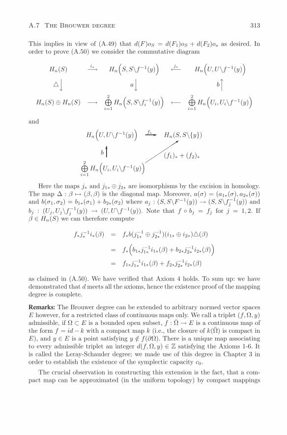
A.7 The Brouwer degree 313
This implies in view of (A.49) that d(F )oS = d(F1)oS + d(F2)os as desired. Inorder to prove (A.50) we consider the commutative diagram
Hn(S) i∗−→ Hn
(S, S\f−1(y)
)j∗←− Hn
(U,U\f−1(y)
)
a
b
Hn(S) ⊕ Hn(S) −→2⊕
i=1
Hn
(S, S\f−1
i (y))
←−2⊕
i=1
Hn
(Ui, Ui\f−1(y)
)
and
Hn
(U,U\f−1(y)
)
2⊕i=1
Hn
(Ui, Ui\f−1(y)
)
Hn(S, S\y)
b
f∗
(f1)∗ + (f2)∗
Here the maps j∗ and j1∗ ⊕ j2∗ are isomorphisms by the excision in homology.The map ∆ : β → (β, β) is the diagonal map. Moreover, a(σ) = (a1∗(σ), a2∗(σ))and b(σ1, σ2) = b1∗(σ1) + b2∗(σ2) where aj : (S, S\F−1(y)) → (S, S\f−1
j (y)) andbj : (Uj , Uj\f−1
j (y)) → (U,U\f−1(y)). Note that f bj = fj for j = 1, 2. Ifβ ∈ Hn(S) we can therefore compute
f∗j−1∗ i∗(β) = f∗b(j−1
1∗ ⊕ j−12∗ )(i1∗ ⊕ i2∗)(β)
= f∗
(b1∗j
−11∗ i1∗(β) + b2∗j
−12∗ i2∗(β)
)
= f1∗j−11∗ i1∗(β) + f2∗j
−12∗ i2∗(β)
as claimed in (A.50). We have verified that Axiom 4 holds. To sum up: we havedemonstrated that d meets all the axioms, hence the existence proof of the mappingdegree is complete.
Remarks: The Brouwer degree can be extended to arbitrary normed vector spacesE however, for a restricted class of continuous maps only. We call a triplet (f,Ω, y)admissible, if Ω ⊂ E is a bounded open subset, f : Ω → E is a continuous map ofthe form f = id− k with a compact map k (i.e., the closure of k(Ω) is compact inE), and y ∈ E is a point satisfying y /∈ f(∂Ω). There is a unique map associatingto every admissible triplet an integer d(f,Ω, y) ∈ Z satisfying the Axioms 1-6. Itis called the Leray-Schauder degree; we made use of this degree in Chapter 3 inorder to establish the existence of the symplectic capacity c0.
The crucial observation in constructing this extension is the fact, that a com-pact map can be approximated (in the uniform topology) by compact mappings
314 Appendix
having their image in finite dimensional subspaces of E. Take such a map k satis-fying k(Ω) ⊂ En ⊂ E, where dim En = n. If x ∈ E is a solution of
(id − k)(x) = 0 ,
then x ∈ En and hence one defines
d(id − k,Ω, 0) = d(id − k,Ω ∩ En, 0) ,
where, on the right hand side, we have the Brouwer degree. This is well-defined.Indeed choosing a larger finite dimensional space Em ⊃ En then d(id − k,Ω ∩En, 0) = d(id − k,Ω ∩ Em, 0). This follows by approximating (id − k)|Ω ∩ Em
by a smooth map having 0 as a regular value and simply computing the indexusing the representation (i) of Proposition 1. Since the finite dimensional mapsare dense in the set of compact maps (in the uniform topology) the continuousmap (id − k,Ω, 0) → d(id − k,Ω, 0) ∈ Z defined above has a unique extension,called the Leray-Schauder degree. For the details we refer the reader to H. Amann[5], K. Deimling [60] and E. Zeidler [232], Chapter 12.
A.8 Continuity property of the Alexander-Spanier cohomology
The mathematical tools needed for Chapter 6 are becoming more sophisticated.In particular, homology and cohomology theory is being used. Besides the basicproperties of a (co-) homology theory the reader needs to know cup products andPoincare duality. All this can be found in standard texts on algebraic topology.We suggest, for example, the book by J. Vick [216], which describes the standardmaterial with great care and also offers an introduction to fixed point theory intro-ducing the fixed point index closely related to degree theory. More comprehensivetreatments on algebraic topology are the books by A. Dold [62], W.S. Massey[148, 149, 150], E. Spanier [203] and R. Switzer [209]. In particular the appendixin [62] concerned with the Kan- and Cech-extension of homotopy invariant func-tors is interesting for the following discussion of continuity properties of homotopyinvariant functors.
Nonlinear analysis is — somewhat exaggerated — the study of nonlinear equa-tions of the form
F (x) = y .
If the map F : X → Y and the topological spaces X and Y have some nice prop-erties, for example, there is some compactness and the solution set is genericallydiscrete, degree theory is a very powerful tool. Sometimes, however, the solutionsets are generically expected to be manifolds and one would like, of course, to knowwhat they are. This is in general a difficult task. But, one can try to compute someof their invariants, using, for example, homology theories. A situation which thenoccurs quite frequently is the following. If we consider the equation F (x) = y we
A.8 Continuity property of the Alexander-Spanier cohomology 315
do not know whether F is generic so that the solution set might be quite badlybehaved, for example, it might not be a manifold. On the other hand, it might bepossible to approximate the solution set F−1(y) by solution sets F−1(yk) which aregeneric, for example, manifolds. In this situation it is sometimes only possible tostudy F−1(yk) by algebraic means (using homology theory) and the question thenis: under which circumstances are we able to conclude something about F−1(y)?
The important tool will be a continuity property for the homology theory,which we discuss in the following. We begin with an abstract discussion which isapplicable in many circumstances and focus on the particular theory we need inChapter 6, namely the Alexander-Spanier cohomology theory, see E. Spanier [203].
Let X be a topological space and C the category of all subspaces, the morphismsϕ : A → B being the continuous maps. Let A be an algebraic category. We considerone of the following cases: A is the category of Abelian groups, or the categoryof commutative rings, or the category of modules over a fixed ring. Assume acontravariant functor h : C → A is given, i.e., to every A ∈ C we associate analgebraic object h(A) ∈ A and to a continuous map ϕ : A → B a homomorphismϕ∗ = h(ϕ) : h(B) → h(A). If A ⊂ B we have a natural inclusion map and wedenote by iAB : h(B) → h(A) the induced map. Since h is a contravariant functorwe have
iABiBC = iAC for A ⊂ B ⊂ C
iAA = Idh(A) .
Given A ⊂ X we denote by OA the collection of all open neighborhoods of A.We denote for U ∈ OA the homomorphism induced by the inclusion A ⊂ U byiU : h(U) → h(A).
Definition 1. Let h be as described above and A ⊂ X fixed. We call h continuousat A if the following conditions hold
(i) Given α ∈ h(A) there exist U ∈ OA and αU ∈ h(U) such that iU (αU ) = α
(ii) Given αU ∈ h(U), with U ∈ OA satisfying iU (αU ) = 0, there exists V ∈ OA
satisfying A ⊂ V ⊂ U and iV U (αU ) = 0.
In other words any element α ∈ h(A) lives already on a neighborhood of A and anyclass α ∈ h(U), U ∈ OA which “dies” on A, “dies” already on some neighborhood.As we shall see in the following we can reconstruct h(A) from the h(U), U ∈ OA
provided h is continuous at A.Observe that OA is a directed set in the following sense. We can define an order
structure ≤ byU ≤ V :⇐⇒ U ⊃ V
(“smaller sets are larger”). Moreover given U, V ∈ OA there exists W ∈ OA
satisfyingW ≥ U ,W ≥ V .
316 Appendix
Indeed, just take W = U ∩ V . Hence we have the following structure. For U ≤ Vwe have a homomorphism
iV U : h(U) −→ h(V )
and for every U ∈ OA a homomorphism
iU : h(U) −→ h(A) .
Moreover, the following holds: If U ≤ V ≤ W then
iWV iV U = iWU and iUU = Id .
Moreover, if U ≤ V , theniV iV U = iU .
We first carry out a construction called the direct limit and then show that it isisomorphic to h(A) provided h is continuous at A.
Define MA ∈ A as the direct sum
MA =⊕
U∈O(A)
h(U) .
If A consists of abelian groups, MA will be an abelian group, etc. Denote by ϕU
the homomorphismϕU : h(U) −→ MA ,
which is the inclusion into the U -th factor.Consider the subgroup, subring or submodule KA generated by elements of the
formϕU (αU ) − ϕV iV U(αU )
where U, V ∈ OA satisfy U ≤ V and where αU ∈ h(U). Define LA by
LA = MA/KA .
Depending on A this quotient is either an Abelian group, or a commutative ringor a module.
Elements of LA are equivalence classes [(αU )] where (αU ) ∈ MA with αU = 0up to finitely many. If αU1 , . . . , αUk
are the non zero elements, then
(αU ) =k∑
i=1
ϕUi(αUi
) .
Let U∞ =⋂k
i=1 Ui. Pick any V ∈ OA, V ≥ U∞. Then for i = 1, . . . , k
βi := ϕUi(αUi
) − ϕV iV Ui(αUi
)
A.8 Continuity property of the Alexander-Spanier cohomology 317
belongs to KA. Consequently,
(αU ) =k∑
i=1
βi + ϕV
( k∑i=1
iV Ui(αUi
))
=: β + ϕV (γ)
where β ∈ KA and γ ∈ h(V ). Hence for every class a ∈ LA there exists Ua ∈ OA
such that for every V ≥ Ua, a is represented by ϕV (αV ) for a suitable elementαV ∈ h(V ). For an element (αU ) ∈ MA we consider the element Φ((αU )) :=∑
U∈OAiU (αU ) ∈ h(A). We note that the sum is finite. For the element
β = ϕU (αU ) − ϕV iV U (αU ) ,
with V ≥ U we compute
Φ(β) = iU (αU ) − iV iV U (αU )
= iU (αU ) − iU (αU )
= 0 .
Clearly Φ : MA → h(A) defines a homomorphism. By the preceding discussion itskernel contains KA. Hence we obtain a homomorphism
Φ : LA −→ h(A) .
In a precise sense Φ gives us what the h(U), U ∈ OA, know about the h(A). Theabove construction is the well-known direct limit denoted by
h(A) := LA = dir limU∈OA
h(U) .
It is an algebraic measure of what the neighborhoods of A know about A withrespect to the contravariant functor h.
Theorem 13. Assume h is continuous at A. Then
Φ : h(A) −→ h(A)
is an isomorphism.
Proof. Assume Φ(a) = 0. We can represent a ∈ h(A) by an element ϕV (αV ) forV ≥ Ua where αV ∈ h(V ) by the preceding discussion. Hence
0 = Φ(a) = iV (αV ) .
By property (ii) of the continuity definition we find W ≥ V such that
αW := iWV (αV ) = 0 .
318 Appendix
Note thatϕV (αV )
= ϕV (αV ) − ϕW iWV (αV )
= ϕV (αV ) − ϕW (αW )
belongs to KA. Hence a = 0. Next let β ∈ h(A). By property (i) there existsU ∈ OA and αU ∈ h(U) with iU (αU ) = β. Let a = [ϕU (αU )]. Then Φ(a) = β.
Assume next that h is a contravariant functor on the category of topologicalspaces. Let X and A be as before and assume Y is another topological space. Iff : X → Y is a continuous map we would like to study f |A : A → Y and saysomething about its properties once we are able to study them for f |U : U → Y ,U ∈ OA. We have the commutative diagram
Y
f |U
f |A
f |V
A
U
V
givingiU (f |U)∗ = (f |A)∗
iUV (f |V )∗ = (f |U)∗ .
We define a homomorphism
f : h(Y ) −→ h(A)
byf(a) = [ϕXf∗(a)] .
We observe that[ϕXf∗(a)] = [ϕU (f |U)∗(a)]
= [ϕU iUXf∗(a)] ,
so that for all U ∈ OA
f(a) = [ϕU (f |U)∗(a)] .
We compute for a ∈ h(U)
Φ f(a) = iU (f |U)∗(a)
= (f |A)∗(a) ,
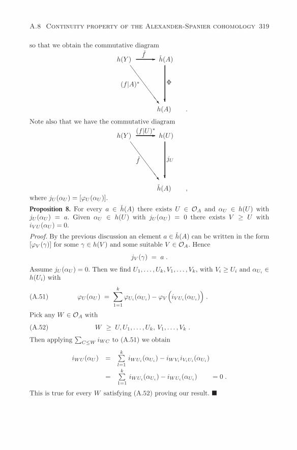
A.8 Continuity property of the Alexander-Spanier cohomology 319
so that we obtain the commutative diagram
h(Y ) h(A)
h(A)
Φ
.
(f |A)∗
f
Note also that we have the commutative diagram
h(Y ) h(U)
h(A) ,
jUf
(f |U)∗
where jU (αU ) = [ϕU (αU )].
Proposition 8. For every a ∈ h(A) there exists U ∈ OA and αU ∈ h(U) withjU (αU ) = a. Given αU ∈ h(U) with jU (αU ) = 0 there exists V ≥ U withiV U (αU ) = 0.
Proof. By the previous discussion an element a ∈ h(A) can be written in the form[ϕV (γ)] for some γ ∈ h(V ) and some suitable V ∈ OA. Hence
jV (γ) = a .
Assume jU (αU ) = 0. Then we find U1, . . . , Uk, V1, . . . , Vk, with Vi ≥ Ui and αUi∈
h(Ui) with
ϕU (αU ) =k∑
1=1
ϕUi(αUi
) − ϕV
(iV Ui
(αUi))
.(A.51)
Pick any W ∈ OA with
W ≥ U,U1, . . . , Uk, V1, . . . , Vk .(A.52)
Then applying∑
C≤W iWC to (A.51) we obtain
iWU (αU ) =k∑
l=1
iWUi(αUi
) − iWViiViUi
(αUi)
=k∑
1=1iWUi
(αUi) − iWUi
(αUi) = 0 .
This is true for every W satisfying (A.52) proving our result.
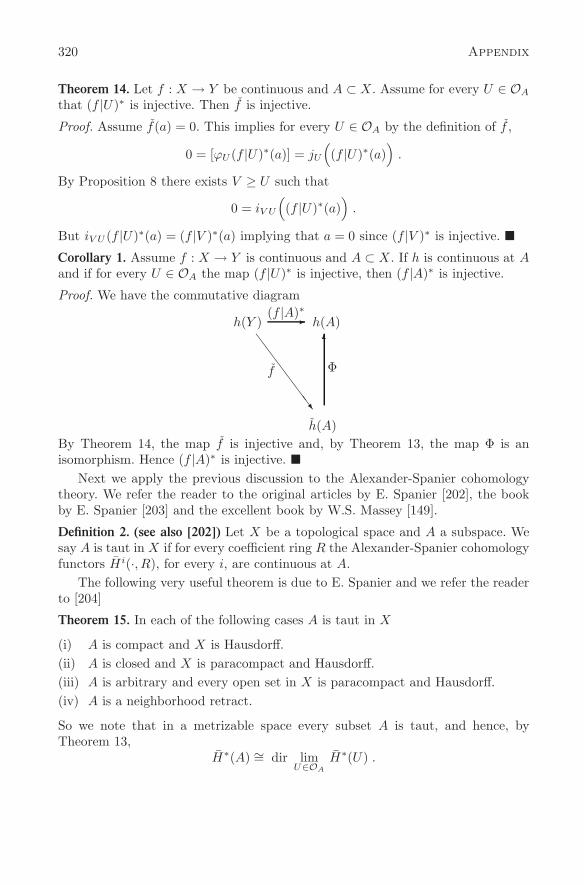
320 Appendix
Theorem 14. Let f : X → Y be continuous and A ⊂ X. Assume for every U ∈ OA
that (f |U)∗ is injective. Then f is injective.
Proof. Assume f(a) = 0. This implies for every U ∈ OA by the definition of f ,
0 = [ϕU (f |U)∗(a)] = jU
((f |U)∗(a)
).
By Proposition 8 there exists V ≥ U such that
0 = iV U
((f |U)∗(a)
).
But iV U (f |U)∗(a) = (f |V )∗(a) implying that a = 0 since (f |V )∗ is injective. Corollary 1. Assume f : X → Y is continuous and A ⊂ X. If h is continuous at Aand if for every U ∈ OA the map (f |U)∗ is injective, then (f |A)∗ is injective.
Proof. We have the commutative diagram
h(Y ) h(A)
h(A)
Φf
(f |A)∗
By Theorem 14, the map f is injective and, by Theorem 13, the map Φ is anisomorphism. Hence (f |A)∗ is injective.
Next we apply the previous discussion to the Alexander-Spanier cohomologytheory. We refer the reader to the original articles by E. Spanier [202], the bookby E. Spanier [203] and the excellent book by W.S. Massey [149].
Definition 2. (see also [202]) Let X be a topological space and A a subspace. Wesay A is taut in X if for every coefficient ring R the Alexander-Spanier cohomologyfunctors Hi(·, R), for every i, are continuous at A.
The following very useful theorem is due to E. Spanier and we refer the readerto [204]
Theorem 15. In each of the following cases A is taut in X
(i) A is compact and X is Hausdorff.(ii) A is closed and X is paracompact and Hausdorff.(iii) A is arbitrary and every open set in X is paracompact and Hausdorff.(iv) A is a neighborhood retract.
So we note that in a metrizable space every subset A is taut, and hence, byTheorem 13,
H∗(A) ∼= dir limU∈OA
H∗(U) .
Index
Abraham, R. and Robbin, J., 291action, 7, 203, 228action of a fixed point, 151action of a periodic solution, 99action spectrum, 151, 152, 186, 269action spectrum, compactness, 152action, bifurcation diagram, 187action-angle coordinates, 273, 278admissible Hamiltonians, 70Alexander-Spanier cohomology,
208, 212, 213, 219almost complex structure, 13–15, 200,
242Ambrosetti, A., 80anti-holomorphic disc, 230Arnold conjecture, 193, 198, 199Arnold conjecture, torus, 202Arnold, V.I., 48, 196, 198, 199, 216, 250,
279Arnold-Jost theorem, 135, 273, 279Arzela-Ascoli theorem, 235, 241asymptotic boundary conditions, 258auxiliary structures, 13Avez, A., 48
Banach manifold W 1,p, 232Bangert, V., 132Banyaga, A., 198Beckner, W., 290Benci, V., 131, 133Bennequin, D., 126Betti numbers, 199, 222bi-invariant metric, 149bi-invariant pseudo-metrics, 150Bialy, M., 186, 187, 190Bialy-Polterovich theorem, 186bifurcation diagram, 187bifurcation diagram, simple, 187, 188Birkhoff invariants, 43, 263Birkhoff normal form, 42, 43, 46Birkhoff’s theorem, 43, 47Birkhoff, G., 42, 47, 131, 194Birkhoff-Lewis theorem, 263
Blanchard, P., 81Bolotin, S.V., 131Bordeaux bottle, 99boundary operator, 256bounded orbits, 205, 234, 236, 253bounded solution, unregularized
flow, 227Bruning, E., 81Brezis, H., 211Brouwer, L., 195, 211Brunella, M., 216bubbling off analysis, 240bundle of anti-linear maps, 232
Calabi invariant, 150canonical basis, 3canonical bi-invariant metric, 149canonical one-form, 128Cantor set, 48cap product, 213capacity preserving
homeomorphisms, 64Cartan’s identity, 11, 13Cauchy-Riemann operator,
224, 242, 253, 291Cauchy-Riemann operator on sections,
295celestial mechanics, 18chain complex, 256, 261chain homomorphism, 259, 267chain homotopy, 259Chang, K.C., 81Chang, S.Y., 290Chaperon, M., 215, 250characteristic line bundle, 22, 113Chekanov, Yu. V., 216Chern-Simons functional, 264Clarke, F., 24classical Hamiltonian systems, 127classical systems, 136classification of symplectic forms, 12closed characteristic, 22, 23closedness of D in C0, 59
321
322 Index
Closing lemma, 21, 105Closing problem, 21cohomology ring, 199commutator, 148compactness of the action spectrum, 152compatible almost complex
structure, 227compatible complex structure, 2compatible inner product, 2complementary symplectic subspaces, 2complex structure, 2, 231computation of Floer homology, 260configuration space, 127conformality axiom, 51conformality of c0, 70Conley’s index theory, 257Conley, C., 198, 200, 203, 215, 221, 258Conley-index, 221Conley-Morse equation, 221Conley-Zehnder theorem, 203connected simple system of C. Conley,
258connecting orbit, 205, 206, 253, 254, 261contact form, 125contact structure, 119, 125contact type, 269contact type hypersurface, 119continuity property of
A.-S. cohomology, 212, 220convex energy surface, 23Courant-Hilbert minimax principle, 39critical points, 205critical value, 79Croke, C., 99cup-length, 199, 216cylinder, 231
Dacorogna-Moser theorem, 31Darboux’s normal form, 12Darboux’s theorem, 10de Rham cohomology group, 12de Rham, G., 12definition of c0, 70definition of c0-Lipschitz type, 116definition of the universal minimax level
γ, 156degree, homological definition, 213determinant, 5
differential forms, 4direct method in the calculus of varia-
tions, 23directed set of admissible pairs, 267displacement energy, 150displacement energy as a special capac-
ity, 172distinguished line bundle, 22Dold, A., 213Douglis, A., 296dual action principle, 31Duistermaat, J.J., 286
Ekeland, I., 31, 33, 51, 59, 61, 66, 99elementary symplectic
transformation, 275Eliashberg conjecture, 169Eliashberg, Y., 59, 123, 126, 150, 201,
216, 269Eliashberg-Gromov theorem, 59Eliasson, H., 232elliptic methods, 222elliptic operator, first order, 225elliptic regularity theory, 227energy, 253energy estimate in C0, 173energy of a symplectic map, 146, 165energy surface, 19energy-capacity inequality, 147, 165Euler characteristic, 198Euler equation, 25Euler-Maupertuis-Jacobi principle, 130existence problem for periodic solutions,
18, 21, 31, 41, 76, 98, 183existence results on prescribed energy
surfaces, 105
Fet, A.I., 131first Chern class, 228, 255flat space, locally, 190Floer complex, 77Floer groups, 262Floer homology, 193, 256, 257Floer, A., 56, 77, 103, 200, 216, 250, 253,
257, 259, 265, 269Floquet multipliers, 110, 111, 135Fomenko, A.T., 286Fortune, B., 201
Index 323
Fourier integral operators, 216Franks, J., 132Fredholm index, 209, 210
Fredholm map, 209Fredholm map, proper, 210Fredholm operator, 298Fredholm theory, 254Fukaya, K., 265fundamental class, 213
Genecand, C., 49
generating function, 13, 189, 273geodesic flow, 130geodesic path in D, 184geodesic path, regular, 185geodesic, length, 186geodesic, minimal, 186, 190Givental, A.B., 216
Gluck, H., 131gluing construction, 256gradient flow, 204, 206gradient-like flow, 206, 217Green’s function, 291Gromov’s squeezing theorem, 33, 55
Gromov, M., 7, 17, 33, 59, 126, 144, 240Gromov-width, 17, 56group of compactly supported symplec-
tic diffeomorphism, 143
Hormander, L., 216Hadamard, J., 131Hamilton-Jacobi equation, 189, 190Hamiltonian diffeomorphism, 198Hamiltonian principle, 23Hamiltonian vector field, 1, 6, 8, 9, 13,
15Hamiltonian, quasi autonomous, 186Herman’s non-closing lemma, 137, 139Herman, M., 105
higher order capacities, 66Hilbert, D., 131Hofer, H., 33, 51, 56, 59, 61, 66, 99, 102,
103, 106, 115, 119, 126, 132,133, 150, 169, 174, 216, 228,250, 253, 262, 265, 269
holomorphic disc, 229holomorphic disc, area, 229
homotopy invariance of Floergroups, 257
Hurewicz homomorphism, 228hypersurface, 19hypersurface of c0-Lipschitz type, 115
inner capacity, 57inner regularity of c0, 70inner regularity of a capacity, 57integrable Hamiltonian system, 46, 134,
278integrals in involution, 46invariance of Hamiltonian vector fields,
13invariance of the symplectic form, 13invariant Lagrangian tori, 48isolated invariant set, 222isotropic subspace, 54
Jacobi metric, 130, 131Jiang, M.Y., 136Joker, 240Jost, R., 279
K.A.M.-theory, 48, 135Kunzle, A., 99kinetic energy, 129Klingenberg, W., 131Kolmogorov, A.N., 48Koslov, V.V., 136Kronecker flow, 47, 48
Lagrangian mechanics, 127Lagrangian submanifold, 216Le Calvez, P., 263Lefschetz fixed point theory, 195Lefschetz, S., 195Legendre transformation, 25length of a symplectic arc, 184Leray-Schauder degree, 96Lewis, D.C., 47Lie derivative, 11limit sets, 217, 218linear canonical map, 4linear symplectic group Sp(n), 5linear symplectic map, 4, 6Liouville form, 128Liouville theorem, 277
324 Index
Liouville, J., 135little trick, 236Ljapunov function, 218, 219Ljapunov-Schmidt reduction, 215Ljusternik Schnirelman theory, 131Ljusternik-Schnirelman, 197, 199, 206,
208, 218, 243Ljusternik-Schnirelman theory, 77localization of Sikorav’s estimate, 178Loewner, C., 196loop space, 203Lutz, R., 126
Ma, R., 103Martinet, J., 126Mather set, 49Mather, J., 49Maupertuis-Jacobi principle, 136Mawhin, J., 81McDuff, D., 267Milnor, J., 211minimax characterisation, 77Minimax lemma, 79Mishchenko, A.S., 286mod 2-degree, 210monotonicity axiom, 51monotonicity of c0, 70monotonicity of the Gromov width, 18Morse complex, 261Morse decomposition, 219, 221Morse equation, 222, 261Morse homology, 261Morse index, 221Morse theory, 31, 77, 131Morse-Smale flow, 257, 261Moser’s deformation method, 12Moser’s theorem, 16Moser, J., 12, 42, 47–49, 135, 198, 263,
286Mountain Pass Lemma, 80
Nekhoroshev, N., 286Nikishin, N., 195Nirenberg, L., 211, 296non-flatness of D, 185nonresonant of order s, 43nontriviality axiom, 51, 57nontriviality of c0, 70
Novikov, S., 262
Offin, D., 134Ono, K., 228, 262orbit of a point, 182order structure on D, 149orthogonal complement, 2orthogonal sum, 3orthogonality, 2osc(H), 146oscillation, 146
P.S.-condition, 78Poschel, J., 48Palais, R., 80Palais-Smale condition, 78parametrized family of energy surfaces,
106parametrized family of
hypersurfaces, 114partial differential equation, 252partial ordering of admissible pairs, 267period group, 228periodic orbit, 18, 23periodic solution, 18perturbation methods, 47perturbations of integrable systems, 47phase function, 216Poincare continuation method, 110Poincare duality, 213Poincare inequality, 27Poincare lemma, 7, 11, 239Poincare polynomial, 199, 221, 261Poincare recurrence theorem, 1, 139Poincare section map, 111Poincare’s recurrence, 263Poincare, H., 19, 21, 110, 194, 197Poincare-Birkhoff fixed point theorem,
194Poincare’s recurrence theorem, 20Poincare, H., 194Poincare-Birkhoff twist theorem, 194Poisson bracket, 43Poisson bracket of two functions, 277Polterovich, L., 150, 186, 187, 190potential energy, 129proper homotopy, 211Pugh, C.C., 21, 139
Index 325
pullback of a form, 4, 6, 12pullback of a vector field, 8
quadratic form, 35quasi autonomous, 186, 187, 190quasi-autonomous, 188, 191quasi-periodic solutions, 47, 48, 50, 135
Rabinowitz, P., 23, 24, 77, 80, 81, 123,133
real filtration of complex, 266recurrence, 19Reeb vector field, 125, 127regular pair (H, J), 255regular value, 211, 212regularity of critical points, 88representation of the gradient flow, 90rescaling, 237rest points, 208, 218Riemannian metric, compatible, 14Riemannian sphere, 231, 232, 294Riesz’ theorem, 77Riesz, F., 77rigidity of symplectic diffeomorphisms,
58rigidity of symplectic embeddings, 51rigidity phenomena, 34Robinson, C., 21, 112, 139Rybakowski, K., 222
Salamon, D., 222, 228, 253, 255, 258,261–263
Sard’s theorem, 119Sard-Smale theorem, 211, 212, 255Schwarz, M., 254, 257, 261Seifert, H., 21, 131set of compatible almost complex struc-
tures, 15set of distinguished Hamiltonians, 70Siburg, K.F., 52, 100Siegel, C.L., 47Sikorav’s estimate, 177Sikorav’s estimate, localized form, 178Sikorav’s theorem, 177, 178Sikorav, J.C., 177, 200, 216, 265Simon, C., 195Smale degree, 210Sobolev class, 232
Sobolev embedding theorem, 241Sobolev space, 82, 203space of compatible almost complex
structures, 15special symplectic capacity, 172standard symplectic space, 4Stein, E., 242Stokes’ theorem, 12, 240Struwe, M., 81, 119symplectic 2-form, 10symplectic action, 7symplectic atlas, 10symplectic basis, 3symplectic capacities of higher order, 66symplectic capacity, 18, 51, 52, 56, 58,
66, 70symplectic capacity c0(M,ω), 265symplectic capacity, definition, 51symplectic capacity, special, 172symplectic classification of open poly-
discs, 269symplectic classification of quadratic
forms, 35symplectic coordinates, 4, 10symplectic diffeomorphism, 6symplectic embeddings, 31symplectic energy, properties, 147symplectic fixed points, 222symplectic group, 5symplectic homeomorphisms, 51symplectic homology, 193, 265symplectic homology groups, 267symplectic homology groups, exact tri-
angle, 268symplectic homology theory, 56, 216symplectic invariants, 18symplectic manifolds, 1, 9symplectic map, linear, 4symplectic maps between manifolds, 12symplectic polar coordinates, 46symplectic structure, 9symplectic structure on a cotangent
bundle, 128symplectic subspace, 3symplectic vector space, 1
Taubes, C., 257Terng, C., 80
326 Index
three-body problem, 21trace-theorem, 287transformation formula for vector fields,
8transformation of a Hamiltonian vector
field, 9transversally hyperbolic, 205Traynor, L., 216
uniformization theorem, 231universal minimax family F , 156universal minimax level γ, 155universal minimax set, 155universal variational principle, 154unparameterized periodic solution, 113unregularized gradient flow
equation, 224, 227
variation of constant formula, 214Vekua, I.N., 298Viterbo’s homological special symplec-
tic capacity, 183Viterbo’s theorem, 123Viterbo, C., 23, 102, 103, 123, 132, 169,
182, 216volume form, 5
weak nontriviality axiom, 51, 66Weierstrass, K., 35Weinstein conjecture, 23, 119, 120, 123,
126, 132Weinstein, A., 23, 24, 42, 99, 120, 123,
198, 201Willem, M., 81Wysocki, K., 269
Yang-Mills action, 264
Zehnder, E., 99, 106, 115, 119, 137, 198,200, 203, 215, 255, 258, 263
Ziller, W., 131
Bibliography
[1] C. Abbas and H. Hofer. Holomorphic curves and global questions in contactgeometry. To appear in Birkhauser.
[2] R. Abraham and J. Robbin. Transversal mappings and flows. W.A. Ben-jamin, Inc., 1967.
[3] B. Aebischer, M. Borer, Ch. Leuenberger, M. Kalin, and H.M. Reimann.Symplectic geometry, an introduction based on the Seminar in Berne 1992.Birkhauser, 1994.
[4] S. Alpern and V.S. Prasad. Combinatorial proofs of the Conley-Zehnder-Franks theorem on a fixed point for torus homeomorphisms. Advances inMathematics, 99:238–247, 1993.
[5] H. Amann. Lectures on some fixed point theorems. Monografias dematematica IMPA, Rio de Janeiro.
[6] A. Ambrosetti and P. Rabinowitz. Dual variational methods in critical pointtheory and applications. J. Funct. Anal., 14:349–381, 1973.
[7] V.I. Arnold. Proof of a theorem of A.N. Kolmogorov on the invariance ofquasiperiodic motions under small perturbations of the Hamiltonian. UspekiMat. Nauk, 18:13–40, 1963. Russian Math. Surveys 18 (1963), 9–36.
[8] V.I. Arnold. Small denominators and problems of stability of motions in clas-sical and celestial mechanics. Uspeki Mat. Nauk, 18:91–196, 1963. RussianMath. Surveys 18 (1963), 85–193.
[9] V.I. Arnold. Sur une propriete topologique des applications globalementcanoniques de la mechanique classique. C. R. Acad. Paris, 261:3719–3722,1965.
[10] V.I. Arnold. Proceedings of Symposia in Pure Mathematics. Mathematicaldevelopments arising from Hilbert problems. AMS, Providence, 28:66, 1976.
[11] V.I. Arnold. Mathematical methods of classical mechanics. Springer-Verlag,Berlin und New York, 1978. In particular: Appendix 9.
[12] V.I. Arnold and A. Avez. Ergodic problems of classical mechanics. W.A.Benjamin, Inc., 1968. In particular Appendix 26.
[13] M. Audin and J. Lafontaine. Holomorphic curves in symplectic geometry.Birkhauser, 1994
327
328 Bibliography
[14] V. Bangert. Geodatische Linien auf Riemannschen Mannigfaltigkeiten. Jber.d. Dt. Math.-Verein., 87:39–66, 1985.
[15] V. Bangert. On the existence of closed geodesics on two spheres. Intern.Journal of Mathematics, 4:1:1–10, 1993.
[16] A. Banyaga. Sur la structure du groupe des diffeomorphismes qui preserventune forme symplectique. Comment. Math. Helvetici, 53:174–227, 1978.
[17] W. Beckner. Sharp Sobolev inequalities on the sphere and the Moser-Trudinger inequality. Annals of Mathematics, 138:213–242, 1993.
[18] V. Benci. Closed geodesic for the Jacobi metric and periodic solutions ofprescribed energy of natural Hamiltonian systems. Ann. Inst. H. Poincare,Analyse non lineaire, 1:401–412, 1984.
[19] V. Benci, H. Hofer, and P. Rabinowitz. A remark on a-priori bounds andexistence for periodic solutions of Hamiltonian systems. NATO ASI Se-ries, Series C, In: Periodic Solutions of Hamiltonian Systems and RelatedTopics,(209):85–88, 1987.
[20] D. Bennequin. Entrelacements et equations de Pfaff. Asterisque, 107–108:83–161, 1983.
[21] H. Berestycki, J.M. Lasry, G. Mancini, and B. Ruf. Existence of multipleperiodic orbits on star-shaped Hamiltonian surfaces. Comm. Pure Appl.Math., 38:253–289, 1985.
[22] M. Bialy and L. Polterovich. Geodesics of Hofer’s metric on the group ofHamiltonian diffeomorphisms. To appear: Duke Math. Journal, 1993.
[23] G.D. Birkhoff. Proof of Poincare’s geometric theorem. Trans. Amer. Math.Soc., 14:14–22, 1913.
[24] G.D. Birkhoff. The restricted problem of three bodies. Rend. Circ. Mat.Palermo, 39:265–334, 1915.
[25] G.D. Birkhoff. Dynamical Systems. Colloquium Publ. A.M.S., Vol. 9, 1927.
[26] G.D. Birkhoff. Stability and the equations of dynamics. Am. J. Math.,49:1–38, 1927.
[27] G.D. Birkhoff and D.C. Lewis. On the periodic motions near a given periodicmotion of a dynamical system. Annali di Math., 12:117–133, 1933.
[28] Ph. Blanchard and E. Bruning. Variational methods in mathematical physics.Springer, 1992.
Bibliography 329
[29] S.V. Bolotin. Libration motions of natural dynamical systems. MoscowUniversity Bulletin, 3, 1978.
[30] Yu.G. Borisovich, V.G. Zvyagin, and Yu.I. Sapronov. Non-linear Fredholmmaps and the Leray-Schauder theory. Russian Math. Surveys, 32(4):1–54,1977.
[31] J. Bourgain. Approximation of solutions of the cubic nonlinear Schrodingerequations by finite-dimensional equations and nonsqueezing properties.IMRN, 2:79–90, 1994.
[32] H. Brezis and L. Nirenberg. Nonlinear functional analysis. In preparation.
[33] L.E.J. Brouwer. Beweis des ebenen Translationssatzes. Math. Ann., 72:37–54, 1912.
[34] M. Brown. A new proof of Brouwer’s lemma on translation arcs. HoustonJ. of Math., 10:35–41, 1984.
[35] M. Brown and W.D. Neumann. Proof of the Poincare-Birkhoff fixed pointtheorem. Michigan Math. J., 24:21–31, 1977.
[36] M. Brunella. On a theorem of Sikorav. L’Enseignement Mathematique,37:83–87, 1991.
[37] T. Carleman. Sur un probleme d’unicite pour les systemes d’equations auxderivees partielles a deux variables independantes. Ark. Mat. Asts. Fys.,26B, No. 17:1–9, 1939.
[38] P.H. Carter. An improvement of the Poincare-Birkhoff theorem. Trans.Amer. Math. Soc., 269:285–299, 1982.
[39] K.-C. Chang. Infinite dimensional Morse theory and multiple solution prob-lems. Birkhauser, 1993.
[40] S-Y. A. Chang. Extremal functions in a sharp form of Sobolev inequality.ICM Berkeley, 1:715–723, 1986.
[41] M. Chaperon. Phases generatrices en geometrie symplectique. In: D.Bennequin, Rencontre entre physiciens theoriciens et mathematiciens enl’honneur de Rene Thom. Publication of the Universite de Strasbourg.
[42] M. Chaperon. Quelques questions de geometrie symplectique. SeminaireBourbaki 1982–83, Asterisque, 105–106:231–249, 1983.
[43] M. Chaperon. Une idee du type “geodesique brisee” pour les systemes Hamil-toniens. C.R. Acad. Sci. Paris Ser. I Math., 298:293–296, 1984. Serie I, no.13.
330 Bibliography
[44] M. Chaperon. Lois de conservation et geometrie symplectique. C.R. Acad.Sci. Paris, 312:345–348, 1991. Serie I.
[45] M. Chaperon and B. D’Onofrio. Sur un theoreme de Claude Viterbo. C.R.Acad. Sci. Paris, 306:597–600, 1988. Serie I.
[46] M. Chaperon and E. Zehnder. Quelques resultat en geometrie symplec-tique. In Seminaire Sud-Rhodanien de Geometrie III: Autour du Theoremede Poincare-Birkhoff, pages 51–121, 1984. Travaux en cours. Hermann Paris.
[47] Yu.V. Chekanov. Legandrova teorija morsa. Uspekhi Mat. Naul., 42:4:129–141, 1987.
[48] A. Chenciner. Sur un enouce dissipatif du theoreme geometrique de Poincare-Birkhoff. C.R. Acad. Sci. Paris, 294, I:243–245, 1982.
[49] A. Chenciner. La dynamique on voisinage d’un point fixe elliptique con-servatif: de Poincare et Birkhoff a Aubry et Mather. Seminaire BourbakiAsterisque, 121/122:147–170, 1984.
[50] A. Floer, H. Hofer and K. Wysocki. Applications of symplectic homology I,to appear in Math. Zeit.
[51] K. Cieliebak, A. Floer, and H. Hofer. Symplectic homology II: A generalconstruction. To appear in Math. Zeit.
[52] K. Cieliebak, A. Floer, H. Hofer, and K. Wysocki. Applications of symplectichomology II. Preprint E.T.H. Zurich (1994).
[53] F. Clarke. A classical variational principle for periodic Hamiltonian trajec-tories. Proc. Amer. Math. Soc., 76:186–188, 1979.
[54] C. Conley. Isolated invariant sets and Morse index. CBMS Reg. Conf. Seriesin Math. 38. AMS, 1978.
[55] C. Conley and E. Zehnder. The Birkhoff-Lewis fixed point theorem and aconjecture of V. I.Arnold. Invent. Math., 73:33–49, 1983.
[56] C. Conley and E. Zehnder. An index theory for periodic solutions of a Hamil-tonian system, volume 1007 of Geometric Dynamics, Lecture Notes in Math-ematics. Springer, 1983. 132–145.
[57] C. Conley and E. Zehnder. Morse type index theory for flows and periodicsolutions of Hamiltonian equations. Comm. Pure Appl. Math., 37:207–253,1984.
[58] C.B. Croke and A. Weinstein. Closed curves on convex hypersurfaces andperiods of nonlinear oscillations. Invent. Math., 64:199–202, 1981.
Bibliography 331
[59] B. Dacorogna and J. Moser. On a partial differential equation involvingthe Jacobian determinant. Ann. Inst. Henri Poincare, Analyse non lineaire,7:1–26, 1990.
[60] K. Deimling. Nonlinear functional analysis. Springer-Verlag, Berlin Heidel-berg, 1985.
[61] W.-Y. Ding. A generalization of the Poincare-Birkhoff theorem. Proc. AMS,88:341–346, 1983.
[62] A. Dold. Lectures on Algebraic Topology. Grundlagen der mathematischenWissenschaften 200, Springer 1980. second edition.
[63] A. Douglis and L. Nirenberg. Interior estimates for elliptic systems of partialdifferential equations. Comm. Pure Appl. Math., 8:503–538, 1955.
[64] J.J. Duistermaat. On global action-angle coordinates. Commun. on Pureand Appl. Math., 33:687–706, 1980.
[65] I. Ekeland. Une theorie de Morse pour les systemes hamiltoniens convexes.Ann. Inst. Henri Poincare, Analyse non lineaire, 1:19–78, 1984.
[66] I. Ekeland. Convexity methods in Hamiltonian mechanics. Springer, 1990.Ergebnisse der Mathematik und ihrer Grenzgebiete, 3. Folge.
[67] I. Ekeland and H. Hofer. Convex Hamiltonian energy surfaces and theirclosed trajectories. Comm. Math. Physics, 113:419–467, 1987.
[68] I. Ekeland and H. Hofer. Symplectic topology and Hamiltonian dynamics.Math. Zeit., 200:355–378, 1990.
[69] I. Ekeland and H. Hofer. Symplectic topology and Hamiltonian dynamicsII. Math. Zeit., 203:553–567, 1990.
[70] I. Ekeland and J.M. Lasry. On the number of periodic trajectories for aHamiltonian flow on a convex energy surface. Ann. Math, 112:283–319,1980.
[71] Y. Eliashberg. A theorem on the structure of wave fronts and its applicationin symplectic topology. Funct. Anal. and its Appl., 21:227–232, 1987.
[72] Y. Eliashberg. Topological characterization of Stein manifolds of dimension> 2. Intern. J. Math., 1:29–46, 1990.
[73] Y. Eliashberg. Filling by holomorphic discs and its applications. LondonMath. Society Lecture Notes, pages 45–67, 1991. Series 151.
[74] Y. Eliashberg. Contact 3-manifolds, twenty year since J. Martinet’s work.Ann. Inst. Fourier, 42:165–192, 1992.
332 Bibliography
[75] Y. Eliashberg and H. Hofer. Unseen symplectic boundaries. In Proceedingsof a Conference in honour of E. Calabi, 1991.
[76] Y. Eliashberg and L. Polterovich. Bi-invariant metrics on the group of Hamil-tonian diffeomorphisms. International Journal of Mathematics Vol. 4, No. 5(1993) 727–738.
[77] Y.M. Eliashberg. Estimates on the number of fixed points of area preservingtransformations. Preprint Syktyvkar 1978 (Russian).
[78] Y.M. Eliashberg. Rigidity of symplectic and contact structures. Preprint,1981.
[79] H. Eliasson. Geometry of manifolds of maps. J. Diff. Geom., 1:169–194,1967.
[80] A. Fahti. An orbit closing proof of Brouwer’s lemma on translation arcs.Enseignement Math., 33:315–322, 1987.
[81] A.I. Fet and L.A. Lusternik. Variational problems on closed manifolds. Dokl.Akad. Nauk. S.S.S.R., 81:17–18, 1951.
[82] A. Floer. Proof of the Arnold conjecture for surfaces and generalizations tocertain Kahler manifolds. Duke Math. J., 53:1–32, 1986.
[83] A. Floer. An instanton invariant for 3-manifolds. Comm. Math. Phys.,118:215–240, 1988.
[84] A. Floer. Morse theory for Lagrangian intersection theory. J. Diff. Geom.,18:513–517, 1988.
[85] A. Floer. The unregularised gradient flow of the symplectic action. Comm.Pure Appl. Math., 41:775–813, 1988.
[86] A. Floer. Cuplength estimates on Lagrangian intersections. Comm. PureAppl. Math., 42:335–356, 1989.
[87] A. Floer, Hofer H., and D. Salamon. Transversality in the elliptic Morsetheory for the symplectic action. Preprint E.T.H. Zurich 1994.
[88] A. Floer, Hofer H., and C. Viterbo. The Weinstein conjecture in P × Cl.
Math. Zeit., 203:355–378, 1989.
[89] A. Floer and H. Hofer. Coherent orientations for periodic orbit problems insymplectic geometry. Math. Zeit., 212:13–38, 1993.
[90] A. Floer and H. Hofer. Symplectic homology I: Open sets in Cn. Math.
Zeit., 215:37–88, 1994.
Bibliography 333
[91] M. Flucher. Fixed points of measure preserving torus homeomorphisms.manuscripta math., 68:271–293, 1990.
[92] O. Forster. Riemannsche Flachen. Heidelberger Taschenbucher. Springer,1977.
[93] B. Fortune. A symplectic fixed point theorem for CPn. Invent. Math.,81:22–46, 1985.
[94] B. Fortune and A. Weinstein. A symplectic fixed point theorem for complexprojective spaces. Bulletin AMS, 12:128–130, 1985.
[95] J. Franks. Periodic points and rotation numbers for area preserving diffeo-morphisms of the plane. Preprint, Northwestern University.
[96] J. Franks. Generalizations of the Poincare-Birkhoff theorem. Ann. of Math.,128:139–151, 1988.
[97] J. Franks. Recurrence and fixed points of surface homeomorphisms. Ergod.Th. and Dynam. Sys., 8:99–107, 1988. Charles Conley Memorial Issue.
[98] J. Franks. A variation of the Poincare-Birkhoff theorem. Amer. Math. Soc.,Providence, 1988. Contemp. Math., 81.
[99] J. Franks. Periodic points and rotation numbers for area preserving diffeo-morphisms of the plane. IHES-Publ.Math., 71:105–120, 1990.
[100] J. Franks. Geodesics on S2 and periodic points of annulus homeomorphisms.Invent. Math., 108:403–418, 1992.
[101] J. Franks. A new proof of the Brouwer plane translation theorem. Ergod.Th. and Dynam. Sys., 12:217–226, 1992.
[102] K. Fukaya. Floer homology for oriented 3-manifolds. Advanced Studies inPure Mathematics, 20:1–92, 1992.
[103] J.M. Gambaudo and P. Le Calvez. Infinite d’orbites periodiques pour lesdiffeomorphismes conservatifs de l’anneau. Preprint, 1991.
[104] C. Genecand. Transversal homoclinic orbits near elliptic fixed points of areapreserving diffeomorphisms of the plane. Dynamics Reported, New Series,2:1–30, 1993.
[105] A.B. Givental. Global properties of Maslov index and Morse theory. Funct.Anal. and its Appl., 22:141–142, 1988.
[106] H. Gluck and W. Ziller. Existence of periodic motions of conservative sys-tems. Princeton University Press, 1983. In: Seminar on minimal submani-folds, E. Bombieri, ed.
334 Bibliography
[107] M. Gromov. Pseudoholomorphic curves in symplectic manifolds. Invent.Math., 82:307–347, 1985.
[108] M. Gromov. Partial differential relations. Ergebnisse der Mathematik.Springer, 1986.
[109] L. Guillon. Le theoreme de translation de Brouwer: une demonstration sim-plifiee menant a une nouvelle preuve du theoreme de Poincare-Birkhoff. 1991.
[110] M.-R. Herman. Differentiabilite optimale et contre-exemples a la fermetureen topologie C∞ des orbites recurrentes de flots Hamiltoniens. ComptesRendus de l’Academie des Sciences. Serie-I.-Mathematique, 313:49–51,1991. No. 1.
[111] M.-R. Herman. Exemples de flots Hamiltoniens dont aucune perturba-tion en topologie C∞ n’a d’orbites periodiques sur un ouvert de sur-faces d’energies. Comptes Rendus de l’Academie des Sciences. Serie-I.-Ma-thematique, 312:989–994, 1991. No. 13.
[112] D. Hilbert. Uber das Dirichlet’sche Prinzip. Jhrb. der Deutschen Math.Vereinigung, VIII, Erstes Heft:184–188, 1900.
[113] M.W. Hirsch. Differential topology. Graduate Texts in Math. 33. Springer-Verlag, 1976.
[114] H. Hofer. Lagrangian embeddings and critical point theory. Ann. Inst. H.Poincare, Anal. Non Lineaire, 2:407–462, 1985.
[115] H. Hofer. Ljusternik-Schnirelman theory for Lagrangian intersections. Ann.Inst. H. Poincare, 5(5):465–499, 1988.
[116] H. Hofer. On the topological properties of symplectic maps. Proceedings ofthe Royal Society of Edinburgh, 115 A:25–38, 1990.
[117] H. Hofer. Estimates for the energy of a symplectic map. Comm. Math. Helv.,68:48–72, 1993.
[118] H. Hofer. Pseudoholomorphic curves in symplectisations with application tothe Weinstein conjecture in dimension three. Invent. Math., 114:515–563,1993.
[119] H. Hofer and D. Salamon. Floer homology and Novikov rings. To appearA. Floer Memorial Volume.
[120] H. Hofer, C. Taubes, A. Weinstein, and E. Zehnder, editors. Floer MemorialVolume. To appear, Birkhauser, 1994.
Bibliography 335
[121] H. Hofer and C. Viterbo. The Weinstein conjecture in cotangent bundlesand related results. Annali Sc. Norm. Sup. Pisa, 15:411–445, 1988. SerieIV, Fasc III.
[122] H. Hofer and C. Viterbo. The Weinstein conjecture in the presence of holo-morphic spheres. Comm. Pure Appl. Math., 45(5):583–622, 1992.
[123] H. Hofer and E. Zehnder. A new capacity for symplectic manifolds, pages405–428. Analysis et cetera. Academic press, 1990. Edit: P. Rabinowitz andE. Zehnder.
[124] L. Hormander. The analysis of linear partial differential operators, volumeI–IV. Springer, Grundlehren Edition, 1983–1985.
[125] M.-Y. Jiang. Hofer-Zehnder symplectic capacity for two dimensional mani-folds. Proc. Royal Soc. Edinb., 123A:945–950, 1993.
[126] R. Jost. Winkel- und Wirkungsvariable fur allgemeine mechanische Systeme.Helvetica Physica Acta, 41:965–968, 1968.
[127] W. Klingenberg. Lectures on closed geodesics. Springer, Grundlehren Math.Wiss. 230, 1978.
[128] A.N. Kolmogorov. The general theory of dynamical systems and classicalmechanics. Proc. Int. Congress of Math. Amsterdam 1954. W.A. Benjamin,Inc., 1967. see Appendix D in R. Abraham: Foundations of mechanics.
[129] V.V. Koslov. Calculus of variations in the large and classical mechanics.Russian Math. Survey, 40:2:37–71, 1985.
[130] S. Kuksin. Infinite-dimensional capacities and a squeezing theorem forHamiltonian PDE’s. Preprint F.I.M., ETH Zurich (1993).
[131] A. Kunzle. The least characteristic action as symplectic capacity. F.I.M.report, ETH Zurich (1991).
[132] K. Kuperberg. A smooth counter example to the Seifert conjecture. Toappear in Annals of Mathematics.
[133] F. Lalonde. Energy and capacities in symplectic topology. Preprint, 1994.
[134] F. Lalonde and D. McDuff. The geometry of symplectic energy. Preprint,1993.
[135] F. Lalonde and D. McDuff. Hofer’s L∞-geometry: energy and stability ofHamiltonian flows I. Preprint, 1994.
[136] F. Laudenbach and J.C. Sikorav. Persistence d’intersections avec la sectionnulle au cours d’une isotopie Hamiltonienne dans un fibre cotangent. Invent.Math., 82:349–357, 1985.
336 Bibliography
[137] H.V. Le and Kaoru Ono. Symplectic fixed points, Calabi invariant andNovikov homology. Max-Planck-Institut Bonn MPI/93–27.
[138] P. Le Calvez. Sur les diffeomorphismes de l’anneau et du tore. Preprint,Universite Paris-Sud.
[139] P. Le Calvez. Une generalisation du theoreme de Conley-Zehnderaux homeomorphismes du tore de dimension deux. PrepublicationsMathematiques de l’Universite Paris-Nord, 93–02, 1993.
[140] P. Le Calvez. Phases generatrices discretes de diffeomorphismes du tore oude l’anneau. Preprint, Unversite Paris-Sud, 1991.
[141] P. Le Calvez. Un theoreme de translations pour les diffeomorphismesdu tore ayant des points fixes. Prepublications Universite de Paris-Sud,mathematiques, 92–85 (1992), 1991.
[142] E. Lima. Orientability of smooth hypersurfaces and the Jordan-Brouwerseparation theorem. Expo. Math., 5:283–286, 1987.
[143] L. Lusternik and L. Schnirelman. Methodes topologiques dans les problemesvariationnels. Herman, Paris, 1934.
[144] R. Lutz. Structures de contact sur les fibres principaux en circles de dimen-sion 3. Ann. Inst. Fourier, 3:1–15, 1977.
[145] A.M. Lyapunov. Probleme general de la stabilite du movement. Ann. Fac.Sci. Toulouse, 2:203–474, 1907.
[146] R. Ma. A remark on Hofer-Zehnder symplectic capacity in M × R2n, 1992.
Preprint, Tsinghua University.
[147] J. Martinet. Formes de contact sur les varietes de dimension 3. Lecture Notesin Math., 209:142–163, 1971.
[148] W.S. Massey. Algebraic topology: an introduction. Graduate Texts in Math-ematics 56. Springer Verlag, 1967.
[149] W.S. Massey. Homology and cohomology theory. Marcel Dekker, Incl. NewYork and Basel, 1978.
[150] W.S. Massey. Singular homology theory. Graduate Texts in Mathematics70. Springer Verlag, 1980.
[151] J. Mather. Existence of quasiperiodic orbits for twist homeomorphisms ofthe annulus. Topology, 21:457–467, 1982.
[152] J. Mawhin and M. Willem. Critical point theory and Hamiltonian systems.Springer, 1989.
Bibliography 337
[153] D. McDuff. Elliptic methods in symplectic geometry. Bulletin AMS,23(2):311–358, 1990.
[154] D. McDuff. Symplectic manifolds with contact type boundaries. Invent.Math., 103:651–671, 1991.
[155] D. McDuff and L. Polterovich. Symplectic packings and algebraic geometry.Preprint, 1993.
[156] D. McDuff and D. Salamon. Introduction to symplectic topology. To appear.
[157] J. Milnor. Topology from the differentiable viewpoint. The University Pressof Virginia, Charlottesville, 1972.
[158] A.S. Mishchenko and A.T. Fomenko. Generalized Liouville method of in-tegration of Hamiltonian systems. Funct. Anal. and its Appl., 12:113–121,1978.
[159] J. Moser. On invariant curves of area preserving mappings of the annulus.Nachr. Akad. Wiss. Gottingen, Math. Phys. Kl., pages 1–20, 1962.
[160] J. Moser. On the volume elements on a manifold. Trans. Amer. Math. Soc.,120:286–294, 1965.
[161] J. Moser. A rapidly convergent iteration method and non-linear partialdifferential equations I and II. Ann. Scuola Norm. Sup. Pisa, 20:265–315,499–535, 1966.
[162] J. Moser. Stable and random motions in dynamical systems. PrincetonUniversity Press, 1973. In: Annals of Math. Studies, Vol. 77.
[163] J. Moser. Periodic orbits near an equilibrium and a theorem of A. Weinstein.Comm. Pure Appl. Math., 29:727–747, 1976.
[164] J. Moser. Proof of a generalized form of a fixed point theorem due to G.D.Birkhoff. Geometry and Topology, Lecture Notes in Mathematics, 597:464–494, 1977.
[165] J. Moser. A fixed point theorem in symplectic geometry. Acta Mathematica,141:17–34, 1978.
[166] J. Moser. Integrable Hamiltonian systems and spectral theory. In LezioniFermiane, Accademia nazionale dei Lincai Scuola Normale Superiore, Pisa,1981.
[167] J. Moser and E. Zehnder. Notes on Dynamical systems. Courant Institute,1980.
338 Bibliography
[168] N. Nekhoroshev. Action-angle variables and their generalization. Trans.Mosc. Math. Soc., 26:181–198, 1972.
[169] N. Nikishin. Fixed points of diffeomorphisms on the two sphere that preservearea. Funkts. Anal. i Prilozhen, 8:84–85, 1974.
[170] S.P. Novikov. Multivalued functions and functionals — an analogue of theMorse theory. Soviet Math. Dokl., 24:222–225, 1981.
[171] D. Offin. A class of periodic orbits in classical mechanics. J. Diff. Eq.,66:90–116, 1987.
[172] K. Ono. On the Arnold conjecture for weakly monotone symplectic mani-folds. Preprint Max-Planck-Institut fur Mathematik MPI/93–4.
[173] R.S. Palais. Critical point theory and the minimax principle. In: GlobalAnalysis. Proc. AMS, XV:185–212, 1970.
[174] R.S. Palais and Terng C.-L. Critical point theory and submanifold geometry,volume 1353. Springer Lecture Notes in Mathematics, 1988.
[175] R.S. Palais and S. Smale. A generalized Morse theory. Bull. AMS, 70:165–171, 1964.
[176] H. Poincare. Methodes nouvelle de la mechanique celeste, volume 3.Gauthier-Villars, Paris, 1899.
[177] H. Poincare. Sur un theoreme de geometrie. Rend. Circolo Math. Palermo,33:375–407, 1912.
[178] J. Poschel. Integrability of Hamiltonian systems on Cantor sets. Comm.Pure Appl. Math., 35:653–696, 1982.
[179] C.C. Pugh and R.C. Robinson. The C1-closing lemma, including Hamilto-nians. Erg. Th. and Dynam. Sys., 3:261–313, 1983.
[180] P. Rabinowitz. Periodic solutions of Hamiltonian systems. Comm. PureAppl. Math., 31:157–184, 1978.
[181] P. Rabinowitz. Periodic solutions of Hamiltonian systems on a prescribedenergy surface. J. Diff. Equ., 33:336–352, 1979.
[182] P. Rabinowitz. Minimax methods in critical point theory with applications todifferential equations. CBMS, Regional Conf. Ser. in Math. 65. AMS, 1986.
[183] C. Robinson. A global approximation theorem for Hamiltonian systems.Proc. Symposium in Pure Math., XIV:233–244, 1970. Global Analysis, AMS.
[184] K.P. Rybakowski. On the homotopy index for infinite-dimensional semiflows.Trans. Amer. Math. Soc., 269:351–382, 1982.
Bibliography 339
[185] K.P. Rybakowski. The homotopy index and partial differential equations.Springer, 1987.
[186] K.P. Rybakowski and E. Zehnder. A Morse equation in Conley’s index theoryfor semiflows on metric spaces. Ergod. Th. and Dynam. Sys., 5:123–143, 1985.
[187] D. Salamon. Connected simple system and the Conley index of isolatedinvariant sets. Trans. Amer. Math. Soc., 291:1–41, 1985.
[188] D. Salamon. Morse theory, the Conley index and Floer homology. Bull.London Math. Soc., 22:113–140, 1990.
[189] D. Salamon and E. Zehnder. KAM theory in configuration space. Comm.Math. Helvetici, 64:84–132, 1989.
[190] D. Salamon and E. Zehnder. Morse theory for periodic solutions of Hamilto-nian systems and the Maslov index. Comm. Pure Appl. Math., 45:1303–1360,1992.
[191] M. Schwarz. Morse homology. Progress in Mathematics, 111. Birkhauser,1993.
[192] P.A. Schweitzer. Counter examples to the Seifert conjecture and openingclosed leaves of foliations. Ann. Math., 100:386–400, 1974.
[193] H. Seifert. Periodische Bewegungen mechanischer Systeme. Math. Zeit.,51:197–216, 1948.
[194] K.F. Siburg. Symplectic capacities in two dimensions. manuscripta math.,78:149–163, 1993.
[195] C.L. Siegel. uber die Existenz einer Normalform analytischer HamiltonischerDifferentialgleichungen in der Nahe einer Gleichgewichtslosung. Math. Ann.,128:144–170, 1954.
[196] C.L. Siegel and J. Moser. Lectures on Celestial Mechanics. SpringerGrundlehren, Band 187, 1971.
[197] J.-C. Sikorav. Problemes d’intersections et de points fixes en geometrieHamiltonienne. Comm. Math. Helv., 62:62–73, 1987.
[198] J.-C. Sikorav. Systemes Hamiltoniens et topologie symplectique. Diparti-mento di Matematica dell’ Universita di Pisa, 1990. ETS, EDITRICE PISA.
[199] J.-C. Sikorav. Homologie associee a une fonctionelle (d’apres A. Floer).Seminaire Bourbaki Exp. 730–744 Asterisque, 201–202–203:115–143, 1991.
[200] C.P. Simon. A bound for the fixed point index of an area preserving mapwith applications in mechanics. Invent. Math., 26:187–200, 1974.
340 Bibliography
[201] S. Smale. An infinite dimensional version of Sard’s theorem. Amer. J. Math.,87:861–866, 1965.
[202] E. Spanier. Cohomology theory for general spaces. Ann. of Math. (2),49:407–427, 1948.
[203] E. Spanier. Algebraic topology. Springer Verlag, New York, 1966.
[204] E. Spanier. Tautness for Alexander-Spanier cohomology. Pacific Journal ofMathematics, (75) 2:561–563, 1978.
[205] E.M. Stein. Singular integrals and differentiability properties of functions.Princeton University Press, 1970.
[206] A. Stephen. On homeomorphisms of the plane which have no fixed points.Abh. Math. Seminar Univ. Hamburg, 30:61–74, 1967.
[207] M. Struwe. Existence of periodic solutions of Hamiltonian systems on almostevery energy surface. Bol. Soc. Bras. Mat., 20:49–58, 1990.
[208] M. Struwe. Variational methods. Springer, 1990.
[209] R. Switzer. Algebraic topology — homotopy and homology. Grundlehren,212. Springer Verlag, Berlin, 1975.
[210] C.H. Taubes. Self-dual Yang-Mills connections on non-self-dual 4-manifolds.J. Diff. Geom., 17:139–170, 1982.
[211] C.H. Taubes. A framework for Morse theory for the Yang-Mills functionals.Preprint Harvard University, 1986.
[212] L. Traynor. Symplectic homology via generating functions. Preprint StanfordUniversity, 1993.
[213] L. Traynor. Symplectic packing constructions. Preprint, 1993.
[214] I. Ustilovsky. Conjugate points on geodesics of Hofer’s metric. Preprint,1993.
[215] I.N. Vekua. Verallgemeinerte analytische Funktionen. Akademie-Verlag,Berlin, 1963.
[216] J. Vick. Homology theory, an introduction to algebraic topology. AcademicPress, 1973.
[217] C. Viterbo. A proof of the Weinstein conjecture in R2n. Ann. Inst. H.
Poincare, Anal. non lineaire, 4:337–357, 1987.
[218] C. Viterbo. Symplectic topology as the geometry of generating functions.Math. Annalen, 292:685–710, 1992.
Bibliography 341
[219] F. Warner. Foundations of differentiable manifolds and Lie groups. Scott,Foresman and Company, 1971.
[220] K. Weierstrass. Mathematische Werke. 1858. Berlin, Band I: 233–246, BandII: 19–44, Nachtrag: 139–148.
[221] A. Weinstein. Contact surgery and symplectic handlebodies. Hokkaido Math.Journal 20 (1990) 241–251.
[222] A. Weinstein. Lagrangian submanifolds and Hamiltonian systems. Ann.Math., 98:377–410, 1973.
[223] A. Weinstein. Normal modes for nonlinear Hamiltonian systems. Invent.Math., 20:47–57, 1973.
[224] A. Weinstein. Lectures on symplectic manifolds, volume 29 of CBMS, Reg.Conf. Series in Math. AMS, 1977.
[225] A. Weinstein. Periodic orbits for convex Hamiltonian systems. Ann. Math.,108:507–518, 1978.
[226] A. Weinstein. On the hypothesis of Rabinowitz’s periodic orbit theorems.J. Diff. Equ., 33:353–358, 1979.
[227] A. Weinstein. On extending the Conley-Zehnder fixed point theorem to othermanifolds. Proc. Sympos. Pure Math., 45, part 2:541–544, 1986. AMS.
[228] F.W. Wilson. On the minimal sets of nonsingular vector fields. Ann. Math.,84:529–536, 1966.
[229] J.C. Yoccoz. Travaux de Herman sur les tores invariants. Bourbaki Exp.745–579, Asterisque, 206:311–345, 1992.
[230] E. Zehnder. Homoclinic points near elliptic fixed points. Comm. Pure Appl.Math., 26:131–182, 1973.
[231] E. Zehnder. Remarks on periodic solutions on hypersurfaces. NATO ASISeries, Series C, In: Periodic Solutions of Hamiltonian Systems and RelatedTopics,(209):267–279, 1987.
[232] E. Zeidler. Nonlinear functional analysis and its applications I. Springer-Verlag, New York Inc., 1986.