The Economics of Food Price Volatility (A National … · This PDF is a selection from a published volume from the National Bureau of Economic Research Volume Title: The Economics

This PDF is a selection from a published volume from the National Bureau of Economic Research

Volume Title: The Economics of Food Price Volatility

Volume Author/Editor: Jean-Paul Chavas, David Hummels, and Brian D.Wright, editors

Volume Publisher: University of Chicago Press

Volume ISBN: 0-226-12892-X (cloth); 978-0-226-12892-4 (cloth); 978-0-226-12892-4 (eISBN)

Volume URL: http://www.nber.org/books/chav12-1

Conference Date: August 15–16, 2012

Publication Date: October 2014

Chapter Title: Influences of Agricultural Technology on the Size and Importance of Food Price Variability

Chapter Author(s): Julian M. Alston, William J. Martin, Philip G. Pardey

Chapter URL: http://www.nber.org/chapters/c12804

Chapter pages in book: (p. 13 – 54)

13

1Influences of Agricultural Technology on the Size and Importance of Food Price Variability

Julian M. Alston, William J. Martin, and Philip G. Pardey

1.1 Introduction

Innovation and technological change in agriculture have contributed to profound changes in the structure of agricultural production, markets, and trade. Significant technological changes have been made both on farms and in the industries that store, transport, process, distribute, and market farm products and supply inputs used by farmers (e.g., see Pardey, Alston, and Ruttan 2010).

These changes have aVected the size and importance of food price vari-ability in three main ways. First, innovations can change the sensitivity of aggregate farm supply to external shocks—for instance, if farmers adopt improved crop varieties that have higher expected yields but more- or less- variable yields, if individual farmers are induced through innovation to

Julian M. Alston is professor in the Department of Agricultural and Resource Economics at the University of California, Davis; associate director of science and technology at the Uni-versity of California Agricultural Issues Center; and a member of the Giannini Foundation of Agricultural Economics. William J. Martin is research manager in agriculture and rural development in the Development Research Group at the World Bank. Philip G. Pardey is pro-fessor in the Department of Applied Economics and director of the International Science and Technology Practice and Policy (InSTePP) Center at the University of Minnesota.

The work for this project was partly supported by the University of California; the University of Minnesota; the HarvestChoice initiative, funded by the Bill and Melinda Gates Foundation; and the Giannini Foundation of Agricultural Economics. The authors gratefully acknowledge excellent research assistance provided by Jason Beddow, Maros Ivanic, Connie Chan- Kang, Kabir Tumber, and Wei Zhang, and helpful comments and advice from various colleagues including Jock Anderson, Steve Boucher, Brian Buhr, Derek Byerlee, Michael Carter, Doug Gollin, Terry Hurley, Travis Lybbert, James Roumasset, Ed Taylor, and Daniel Sumner, as well as Jim MacDonald and other participants at the NBER conference. For acknowledgments, sources of research support, and disclosure of the authors’ material financial relationships, if any, please see http://www.nber.org/chapters/c12804.ack.

14 Julian M. Alston, William J. Martin, and Philip G. Pardey

become more specialized in particular outputs, or if the adoption of innova-tions results in less variation among farmers in the timing of farm operations (e.g., the date of planting of crops) or an increase in the geographical con-centration of production. Second, technological innovations on or oV farms can result in changes in the price elasticity of supply or demand (of both farm inputs and outputs), changing the sensitivity of prices to a given extent of underlying variability of supply or demand or both. This can happen both directly, as a consequence of particular innovations, or indirectly because of the broader economic implications of technological changes—for example, by increasing incomes. Third, food price volatility is less important to richer people and, by increasing the general abundance of food and reducing the share of income spent on food, agricultural innovation has made a given extent of volatility less important.

The recent evidence of a slowdown in agricultural productivity growth in many parts of the world, combined with the rise of biofuels, has coin-cided with a reversal of the trend of rising abundance of food, and a cor-responding increase in vulnerability of a greater number of poor people to food price volatility.1 Moreover, as poor farmers respond to food scarcity by increasing the intensity of production practices and moving farther into marginal areas, we may see an increase in vulnerability of their production to weather and other shocks for some farmers. This chapter explores these diVerent dimensions of the role of agricultural technology in contributing to or mitigating the consequences of variability in agricultural production, both in the past and looking forward.

1.2 A Simple Model of Technology and Prices

A simple supply and demand model can be used to illustrate the various ways in which changes in technology influence food price variability.2 In the following model of the farm- level market for a staple food commodity, subscripts s and d refer to supply and demand respectively, Q represents quantity, P represents price, and η represents the absolute value of the elas-ticity of supply or demand.3 In each equation, α, the “intercept” comprises a deterministic part and a random part, which is the source of variability:

1. Whether measures of growth of total factor productivity (TFP) or multifactor productivity (MFP) in agriculture are exhibiting a slowdown is the subject of a continuing debate among agricultural economists, but the participants in that debate have agreed that growth rates of partial factor productivity measures such as crop yields have slowed for the world as a whole and for most producing countries (e.g., see Alston, Babcock, and Pardey 2010).

2. Although the general discussion is pertinent to a broader set of circumstances, for con-creteness we have in mind a model of the national or global market for a particular food com-modity, as represented by aggregate farm- level annual supply and demand. To emphasize the important first- round eVects the analysis is mainly partial, although the empirical simulations in section 1.5 explicitly link the farm sector to the broader economy.

3. Some more- detailed results will be conditioned by the use of constant elasticity forms as a local approximation to represent supply and demand equations that could take some other shape, but the main results here will not be sensitive to this approximation, which allows us to represent the key relationships in terms of familiar parameters.

Influences of Agricultural Technology on Food Price Variability 15

(1) lnQs = s + s lnPs (supply)

(2) lnQd = d - d lnPd (demand)

Assuming Qs = Qd and Ps = Pd , solving equations (1) and (2) for market clear-ing prices and quantities yields:

(3) lnP = (d - s)/(s + d),

(4) lnQ = (sd + ds)/(s + d).

Taking variances of ln P and ln Q in equations (3) and (4) yields:4

(5) Var(lnP) = [Var(d) + Var(s) - 2Cov(d,s)]/(s + d)2,

(6) Var(lnQ) = [d2Var(s) + s

2Var(d) + 2sdCov(d,s)]/(s + d)2.

Hence, price volatility, as represented by the variance of logarithms of prices in equation (5), increases with either (a) increases in the variability of demand or supply, as represented by Var(d) and Var(s); (b) reductions in the covariance between shocks to supply and demand; or (c) decreases in the elasticity of supply or demand. The corresponding measure of quantity variability in equation (6) increases with increases in variability of supply or demand or decreases in the covariance, but the signs of the eVects of the elasticities depend on their relative sizes and the relative sizes of the variance and covariance terms.

Technology enters equations (5) and (6) in several ways, both on the demand side and the supply side. Specifically, the intercepts ( s and d ) and elasticities ( s and d) are all functions of technology along with other vari-ables, which are also left implicit, some of which may interact with technol-ogy and modify its eVects on price volatility. In many contexts, for practical purposes the covariance terms in equations (5) and (6) will be negligible.5 On the other hand, the mechanization of agriculture, the introduction of chemical fertilizers, and the rise of biofuels have tended to make the supply and demand for agricultural products more elastic (agriculture using a larger share of highly elastically supplied petroleum- based products as inputs makes supply more elastic, and biofuels demand makes demand for agricul-tural products more elastic unless it is driven by binding mandates). These factors also make agricultural supply and demand potentially more variable (because they are now vulnerable to oil price shocks in a way that was not true in the era of the horse), and the linkage of agriculture to the oil economy

4. Alternative measures of variability were considered. Many studies have used a coeY-cient of variation to remove the influence of diVerences in average levels or in units of mea-surement (e.g., Hazell 1989; Gollin 2006). The variance of log- transformed data has similar characteristics—it is unit- free and invariant to multiplicative transformations of the data—and has the further advantage that statistical tests developed for comparing variances between populations can be applied directly to it, as discussed by Lewontin (1966).

5. Sudden health epidemics, like bird flu or SARS, aVect demand and could also aVect supply if the aVected labor is a major input into agricultural production, as it is in economies with agriculturally oriented economies and labor- intensive farming systems.


makes for a negative covariance between demand shocks and supply shocks (higher oil prices increase demand for biofuels and reduce agricultural supply). Much of the motivation for the present interest in commodity price volatility relates to this nexus. Table 1.1 summarizes the channels by which changes in technology can aVect price variability as expressed in equation (5). The discussion that follows puts flesh on these bones.

1.2.1 On- Farm Agricultural Technology and Price Variability— The Supply Side

The primary role of technical change in agriculture has been to increase the supply of farm commodities, which we can think of as a decrease in the intercept of the supply equation, s in equation (1), reflecting a downward (or outward) shift in supply stemming from the use of new and better farm-ing techniques or inputs.6 As a result of innovations of this nature, global growth in supply over the second half of the twentieth century significantly outpaced growth in demand, arising mainly from growth in population and income, to the extent that since 1975 real prices of cereals have fallen by roughly 60 percent (see appendix A). These changes in turn have changed the implications for farm and nonfarm families of a given extent of price variability, an issue to which we will return later. They may have also served to change the extent of price variability as discussed next.

More variable supply of farm outputs? Clearly on- farm innovations (and other changes, some of which were not simply changes in technology, such as a change in the structure, size, and specialization of farms) have pro-foundly changed the supply function. As well as changing the position of the supply function, the same innovations may have entailed changes in the vulnerability of farm production to biotic and abiotic stresses, reflected as changes in Var(s). A widespread view of technological innovation is that it leads to the introduction of monocultures that—while higher yielding—are more vulnerable to output shocks from disease or other sources. Some economists have proposed that “Green Revolution” technology, for instance, increased cereal yields on average but also led to increases in relative yield variability for individual producers or in aggregate (e.g., Hazell 1989).7 How-ever, more recent studies have tended to find that Green Revolution technol-

6. Much of what we refer to here as “on- farm” technology is developed and produced “oV- farm” for adoption by farmers. These on- farm innovations (including seeds, chemical fertilizers and pesticides, machinery, and methods not embodied in physical inputs) themselves reflect important changes in technology used by the agribusiness firms that supply inputs used by farmers—including everything from ballpoint pens and telephones through to satellite navi-gation systems, the Internet, and everything in between, which are also used by farmers. OV- farm technologies also include the technologies to process farm output, which may change the composition of and intensity of farm output used in food, fiber, feed, and fuel products.

7. Even if yield variance does not increase for individual farmers, an increased covariance of yield (or yield risk) among farmers implies an increase in variance of production and prices globally.

Tab

le 1

.1

Cha

nnel

s th

roug

h w

hich

agr

icul

tura

l and

oth

er te

chno

logy

aff

ects

food

pri

ce v

aria

bilit

y

Par

amet

er in

eq

uati

on 5

EV

ect o

n pr

ice

vari

abili

ty

Typ

e of

tech

nolo

gica

l cha

nge

and

exam

ples

Var

iabi

lity

of s

uppl

y of

farm

pro

duct

:

Var

(αs)

+O

n- fa

rm te

chno

logy

• N

ew c

rop

vari

etie

s: e

.g.,

Bt m

aize

is le

ss v

ulne

rabl

e to

ext

rem

e pe

st p

ress

ure

• G

reen

Rev

olut

ion

tech

nolo

gies

usi

ng m

oder

n va

riet

ies

wit

h m

oder

n in

puts

(fer

tiliz

er, i

rrig

atio

n) h

ave

less

- var

iabl

e yi

elds

• In

tegr

ated

pes

t man

agem

ent a

llow

s be

tter

- inf

orm

ed d

ecis

ions

that

red

uce

vuln

erab

ility

to p

ests

and

dis

ease

s•

Mec

hani

zati

on r

educ

es v

ulne

rabi

lity

to fa

rm la

bor

shor

tage

s; in

crea

ses

vuln

erab

ility

to s

ome

wea

ther

sho

cks

• O

ther

tech

nolo

gy- i

nduc

ed c

hang

es in

inpu

t mix

may

incr

ease

impo

rtan

ce o

f in

puts

wit

h m

ore

vari

able

sup

ply

• In

tens

ive

lives

tock

pro

duct

ion

may

be

mor

e vu

lner

able

to d

isea

se c

onta

gion

but

bet

ter

able

to c

onta

in o

utbr

eaks

T

echn

olog

y- in

duce

d ch

ange

s in

loca

tion

of

prod

ucti

on•

Shif

t of

geog

raph

ic lo

cus

of p

rodu

ctio

n to

pla

ces

wit

h di

Ver

ent c

limat

e or

oth

er fa

ctor

s th

at in

fluen

ce v

aria

bilit

y P

re- f

arm

tech

nolo

gy•

New

tech

nolo

gy (e

.g.,

tran

spor

tati

on, m

anuf

actu

ring

) may

influ

ence

var

iabi

lity

of s

uppl

y of

fact

ors

to fa

rmer

sE

last

icit

y of

sup

ply

of fa

rm p

rodu

ct:

η s

–M

ore

elas

tic

supp

ly o

f fa

rm p

rodu

cts

coul

d re

sult

from

cha

nges

in p

re- f

arm

or

on- f

arm

tech

nolo

gy•

Incr

ease

d us

e of

mor

e el

asti

cally

sup

plie

d in

puts

—e.

g., i

nten

sive

live

stoc

k pr

oduc

tion

use

s fe

ed g

rain

s•

Indu

ced

redu

ctio

ns in

rel

ativ

e im

port

ance

of

hom

e co

nsum

ptio

n re

duce

the

elas

tici

ty o

f su

pply

of

mar

keta

ble

surp

lus

• Im

prov

ed o

n- fa

rm s

tora

ge te

chno

logy

incr

ease

s el

asti

city

of

supp

ly to

the

mar

ket

Var

iabi

lity

of d

eman

d fo

r fa

rm p

rodu

ct:

V

ar(α

d)

+C

hang

es in

pos

t- fa

rm te

chno

logy

(st

orag

e, p

rese

rvat

ion,

tran

spor

t, h

andl

ing,

pro

cess

ing,

food

man

ufac

turi

ng, m

arke

ting

)•

Impr

oved

sto

rage

and

pre

serv

atio

n te

chno

logy

like

ly to

red

uce

vari

abili

ty o

f de

man

d T

echn

olog

y th

at a

llow

s m

arke

ts to

be

bett

er- i

nteg

rate

d ov

er s

pace

and

tim

e•

Can

mak

e m

arke

t vul

nera

ble

to g

over

nmen

t int

erve

ntio

n (t

rade

bar

rier

s, “

stab

iliza

tion

” po

licie

s)•

May

incr

ease

the

risk

of

vola

tilit

y fr

om e

Vec

ts o

f in

vasi

ve p

ests

and

dis

ease

sE

last

icit

y of

dem

and

for

farm

pro

duct

:

η d

–C

hang

es in

pos

t- fa

rm te

chno

logy

cou

ld m

ake

dem

and

for

farm

pro

duct

s m

ore

elas

tic

• T

echn

olog

y th

at a

llow

s m

arke

ts to

be

bett

er in

tegr

ated

ove

r sp

ace

and

tim

e m

akes

dem

and

mor

e el

asti

cC

hang

es in

on-

or

off-

farm

tech

nolo

gy c

ould

mak

e de

man

d fo

r fa

rm p

rodu

cts

less

ela

stic

•

Tec

hnol

ogy

that

con

trib

utes

to in

crea

ses

in p

er c

apit

a in

com

es m

akes

dem

and

for

food

com

mod

itie

s le

ss e

last

icC

ovar

ianc

e of

sup

ply

and

dem

and

shoc

ks:

C

ovar

(αd,

α s)

–

Var

ious

tech

nolo

gies

incr

ease

the

stre

ngth

of

the

link

betw

een

agri

cult

ure

and

oil p

rice

s an

d in

crea

se th

e co

vari

ance

bet

wee

n de

man

d an

d su

pply

sho

cks

affe

ctin

g ag

ricu

ltur

e•

Incr

ease

d us

e of

mec

hani

cal t

echn

olog

ies

and

petr

oleu

m- b

ased

inpu

ts s

uch

as c

hem

ical

fert

ilize

rs•

Incr

ease

d pr

oduc

tion

of

biof

uels

Not

e: T

he s

ymbo

l + in

dica

tes

a po

siti

ve e

Vec

t of

an in

crea

se in

the

para

met

er o

n va

riab

ility

of

food

pri

ces,

and

the

sym

bol –

indi

cate

s a

nega

tive

eV

ect.


ogies reduced the relative variability of maize and wheat yields over time (e.g., as suggested by Gollin 2006).

A more subtle but still substantial influence is that changes in technology have contributed to changes to where production takes place—for instance, enabling wheat production to shift from the eastern United States into the Great Plains states and north into Canada (e.g., see Olmstead and Rhode 2002, 2010)—with implications for variability of yield and production.8 More recently Beddow (2012) estimated that from 1899 to 2007 the centroid of corn production—essentially the geographical pivot point of US corn production—moved about 440 kilometers in a northwesterly direction. In 1899 the centroid of production was located in central Illinois; by 2007 it had migrated to southeastern Iowa.

On the other hand, some new technologies have equipped farmers to better match technology to environments, to make them potentially less vulnerable to stresses, or to be more resistant to some types of stress. The most recent revolution in crop varietal technology uses genetically modified (GM), herbicide- tolerant (HT), or insect- resistant (IR) varieties that substi-tute for chemical pesticides. These varieties change the yield profile of the crops in ways that have specific implications for variability of production. In particular, insect- resistant varieties avoid the severe yield losses that can arise with conventional technology in seasons with extreme pest pressure, espe-cially in those areas where access to chemical pesticides is limited. Unlike the chemical pesticide technologies they substantially replace in many set-tings, yields of genetically engineered insect- resistant crop varieties are less vulnerable to insect damage because the technology does not rely on farmers anticipating pest problems and spraying in advance or observing infestations and spraying when they are under way (Qaim and Zilberman 2003; Hurley, Mitchell, and Rice 2004).9 The insecticide is inherent in the plant.

In a similar vein, integrated pest management (IPM) technologies involve monitoring pest populations and applying pesticides at an optimal rate and time according to pest pressure, rather than according to the calendar. These and other information technologies allow farmers to apply inputs more flex-ibly and more precisely in ways that can reduce vulnerability to both biotic and abiotic stresses. Further, thinking more broadly about the change in paradigms associated with technological advance, we have improved meth-ods for the early detection and management of pests and diseases using both

8. Beddow et al. (2010) document dramatic shifts in the location of agricultural production around the world during recent decades.

9. From the evidence presented by Hurley, Mitchell, and Rice (2004) it is evident that Bt corn technologies unambiguously reduced the relative variability of crop yields. However, the eVects on the variability of corn supply could be ambiguous, depending on the fee charged for the use of the Bt technology. Qaim and Zilberman (2003) reported significant reduction in pest damage and higher average yield for Bt cotton in India; their results would also appear to imply reduced variance of yields.


current technology on farms and induced adaptive innovation as private and public research institutions respond to information about pest and disease threats.

More elastic supply of farm outputs? Second, technical change on farms may have resulted in changes in the elasticity of supply of agricultural out-puts and the food, feed, fuel, and fiber products derived from agricultural outputs. One way this can happen is if new technologies emphasize the use of inputs that are relatively elastically supplied, such as agricultural chemi-cals, energy inputs, seed, or agricultural machinery (or, more precisely, the services from them), rather than inputs that are comparatively inelastically supplied, such as land and water, and in some cases, labor (see, for example, Schultz 1951). If relatively elastically supplied inputs represent an increased share of the cost of production, then the elasticity of supply will be greater (e.g., see Muth 1964); likewise, supply will be made more elastic if an innova-tion allows greater substitutability among inputs.

In the US poultry and hog industries, for instance, the introduction of intensive production systems made supply comparatively elastic. The pri-mary inputs are feed grains and oilseeds, which are highly elastically sup-plied to each of these industries; there are not really any constrained spe-cialized factors of production, and the producing units are replicable at eYcient size such that the industry is characterized by constant returns to scale. In the richer countries at least, this industrial structure replaced an industry based on smaller, less- specialized operations, in which hogs and poultry were often raised as sidelines on dairy and grain- producing farms. As documented by Key and McBride (2007) and MacDonald and McBride (2009), livestock agriculture in the United States has undergone a series of striking transformations that aVected the structure of the industry and the nature of supply response. Production has become more specialized, such that nowadays farms usually confine and feed a single species of animal, often with feed that has been purchased rather than grown on site, and they typically specialize in a specific stage of production. The scale of operations has increased, and economies of scale have contributed along with techno-logical innovations to rapid growth of productivity. Contracting over pro-duction and the use of hired labor have both grown in importance.10 Similar innovations have taken place in many other countries and are underway in others. These innovations that have tended to make livestock supply in these markets more elastic (at least over the medium to long run), might at the same time have made production more (or less) vulnerable to shocks such as

10. These technical changes have coincided with the move toward the pervasive use of con-tract farming and vertically integrated structures in most rich- country livestock supply chains. These institutional and structural developments may have muted short- run quantity responses to changes in market prices for farm commodities because of fixities in these complex supply systems, while enabling greater medium- to long- run response to price changes.


disease epidemics that may be spread more rapidly within closely confined systems, but they might also be easier in some cases to prevent, detect, and contain for similar reasons and given the use of better hygiene and access to improved veterinary medicines and practices.

Another way in which changes in technology on farms may have aVected the elasticity of supply to the market is by changing the cost of on- farm stor-age or by causing (through eVects on incomes, the extent of specialization, or other variables) changes in the importance of farm- household consumption as a share of the total use of farm output. The elasticity of supply of market-able surplus is an inverse- share- weighted average of the elasticity of farm production response with respect to price and the (absolute) elasticity of farm- household consumption response to price, such that changes in tech-nology that reduce the relative importance of farm- household consumption will tend to reduce the elasticity of supply to the market.

In principle, changes in technology in the agribusiness sector that supplies inputs used by farmers might aVect the variability in supply of key inputs, or the elasticity of supply of key inputs, to an extent that either the elastic-ity of farm output supply or the variability of farm output supply would be aVected. For example, the rise of genetically engineered proprietary seed technologies represents an instance where a change in the technology of crop varieties (i.e., genetic engineering) has given rise to a substantial change in the conditions of input supply to the industry. Seed costs now represent a significant share (say, 10 percent) of total costs in North American corn, cotton, canola, and soybean production (e.g., see Alston, Gray, and Bolek 2012), with the technology supplied by a relatively concentrated sector with monopoly privileges. These developments in the conditions of seed supply might have implications for variability in supply in addition to those implied by the seed technology itself given their important consequences for the cost shares of diVerent categories of inputs and the process by which input prices are determined.

1.2.2 Postfarm Agricultural Technology and Price Variability

Changes in technology in the postfarm agribusiness sector might change the elasticity of demand or the variability of demand, or both, as well as contributing to the growth of demand for farm outputs. The characteristics of demand for the farm product might also be aVected by on- farm changes in technology that have had profound eVects on incomes of the poor, which would be expected in turn to contribute to increases in demand for most farm products (though with a shift in the balance toward livestock prod-ucts), and to make demands for farm commodities generally less elastic, and perhaps less variable.

The main factors driving growth in demand for farm products have been changes in the share and structure of on- versus oV- farm consumption


(associated with increases in farm size and specialization, part- time farm-ing and urbanization), and increases in population and per capita incomes. The same factors have influenced the structure of demand. As per capita incomes rise, a greater share of food is consumed away from home or in more- processed and more- convenient forms for within- home consumption (e.g., Senauer, Asp, and Kinsey 1991). This reduces the farm component of retail food costs, thus muting the food price eVects of fluctuations in farm- level commodity prices. All of these factors have been driven to some extent by on- farm innovations, which made food much cheaper while increasing farm incomes and freeing up labor, hitherto used on farms, for other pur-suits. Complementary changes in technology oV the farm have included improved technology for processing, storing, preserving, and handling food products, which, from the farmers’ perspective, are also manifest as increases in demand.

Transportation and storage (notably refrigeration) technologies that increased demand for farm commodities also served to integrate markets over space and time.11 Our simple market model abstracts from these rela-tionships, but we can easily imagine what would happen if we expanded it from one country to two countries. In a two- country model, if we introduce trade (as a result of improved technology, increasing eVective price trans-mission) we will make the eVective demand (and supply) for food commodi-ties facing each country more elastic, and we will make the prices in each country less variable, compared with the autarky prices, unless the shocks that are the sources of variability are perfectly correlated between the two countries. From this perspective, technology that improves transportation, facilitating interregional and international trade, would be expected to serve to reduce price variability unless it somehow increases the correlation of shocks between countries.12

While freer international trade in commodities does allow arbitrage to play its role in buVering prices from supply or demand shocks, it also facili-tates the international movement of pests and diseases that could contribute to increases in volatility—for instance, the losses already experienced from the citrus greening disease Huanglongbing (known as HGB, and spread by the Asian citrus psyllid), which is already a serious problem in Brazil and now threatens the US citrus industry. Of course, the Columbian Exchange was necessary to create the possibility of “antigains” from trade in citrus

11. Information technologies that make for more eYcient markets, including futures and options markets as well as spot markets, should play a complementary role in facilitating markets to better anticipate and absorb or accommodate shocks, and in enabling individuals to cope better generally with variability.

12. However, closer market integration means prices of individual inputs and outputs are more closely correlated spatially and this may have contributed to an increased covariance in prices of outputs both of the same crops among places and across crops. In turn this would add to the variance of production and prices.


and other crops by North America today, so the counterfactual is not easy to make sensible, but the point is that trade has sometimes made food prices both less volatile in the normal short- run sense and potentially more volatile in a longer- run sense because of the concomitant increases in the risk of losses from exotic pests and diseases.13

A more subtle implication is introduced when we consider the role of government. While international and interregional trade enabled by innova-tions in product preservation and transport technologies may have reduced on- and oV- farm price variability ceteris paribus, it also creates new possi-bilities for government intervention in trade. Government intervention can make price variability worse, and it can do so in ways that are particularly damaging (such as active interventions in times of price spikes—e.g., see Martin and Anderson [2012]). The combined eVect of trade and govern-ment could conceivably make volatility worse compared with autarky, an outcome that would not have happened without the creation of trade facili-tated by technology. A similar argument applies in the context of improved storage technologies, which enable prices and consumption to be smoothed over time, and thereby generate net social benefits. But the development of storage technologies also enabled governments to introduce buVer stock schemes, which have historically proven to be very expensive policies. The Australian wool industry fiasco in the late 1980s is a telling example. Massy (2011) estimated that the collapse of the wool reserve price scheme in 1991 imposed social costs worth at least AU $12 billion at today’s prices, more than five times the recent annual gross value of Australian wool production. Of course, the main issue here is not the storage or transport technology itself; rather, it is the unhappy decisions made by governments. But technol-ogy is involved and conditions the possibilities for damaging or desirable government policies.

Much could be said about technologies for food processing and preserva-tion, but we will restrict attention here to fermentation technology (see Zil-berman and Kim 2011). Fermentation has served as a means of converting perishable food products—such as fruit, grain, milk, and vegetables—into less perishable, more palatable, and safer forms—such as wine, beer, cheese, yogurt, sauerkraut, and kimchi among others. It also has enabled the trans-formation of food commodities into biofuels products. The net implications of these manifold changes are diYcult to decipher, but of great immediate interest is the consequential linking of food commodity markets to fossil fuel and thus the broader economy in new ways that surely will have implications for food price volatility.

13. The widespread exchange of animals, plants, culture, human populations, communicable disease, and ideas between the American and Afro- Eurasian hemispheres following the voyage to the Americas by Christopher Columbus in 1492 is known as the “Columbian Exchange.”


1.3 EVects of Technology on the Implications of Price Variability

As noted, the most important eVects of changes in technology are through their cumulative eVects on reducing the expected value of prices, rather than their impacts on price variability. By increasing real incomes through higher producer incomes at any given price and lower costs of living, and by inducing and enabling some people to leave production agriculture, technol-ogy changes the welfare implications of agricultural variability. A simple heuristic model can be used to illustrate how this works.

1.3.1 Elements of Benefits and Determinants of Beneficiaries

Productivity- enhancing changes in technology for the production of a staple crop give rise to benefits ( Bi), accruing to the ith household, approxi-mately equal to

(7) Bi = -PiCi lnPi + (ki + lnPi)PiQi,

where Pi is the price paid by the household for its consumption, Ci (and received for its production, Qi) of the crop, and ki is its household- specific proportional cost reduction associated with the improvements in technology giving rise to the proportional price change, lnPi < 0. The first element of the equation represents the consumer benefit. Households that consume but do not produce the crop obtain a benefit equal to the reduction in their cost of consumption—a real income eVect of the research- induced price fall. The second element represents the producer benefit. Households that pro-duce but do not consume the crop obtain a gain equal to the diVerence between their proportional cost reduction and the proportional fall in price

(ki + lnPi ) times the value of their production.More generally, households that both produce and consume the good

receive a net gain equal to the sum of two gains, as shown in the following version of the above equation:

(7′) Bi = kiPiQi - (PiCi - PiQi ) lnPi.

The first term in equation (7′) is the household’s cost saving on produc-tion (their proportional cost saving times their value of production). The second is their gain from the reduction in their net costs of food purchases (the diVerence between their expenditure on consumption and the value of their production) resulting from the fall in price. The size of the first term in equation (7′) will depend on the nature, as well as the size, of the shift in technology (Martin and Alston 1997). For food deficit households, the fall in price means a benefit; for food surplus households, it means a loss. Gain-ers include all households who produce less of the good than they consume, regardless of whether they adopt the new technology or not. Potential losers are those surplus households (i.e., who produce more than they consume)


that are not able to achieve a per unit cost reduction equal to the market- wide reduction in price associated with the technology. Among these, in this analysis, those surplus households that are unable to adopt the technology are the only sure net losers. Some of these households might be induced to leave agriculture and find employment elsewhere.14

The above analysis might be interpreted as a medium- term or partial analysis. A more general or longer- run analysis could take more explicit account of linkages with the broader economy and this might change the story. Gardner (2002, 328–333) presented evidence that, over a thirty- year period 1960 to 1990, changes in average county- level US farm household incomes were not related to changes in agricultural productivity (or any other agriculture- specific variable). The general idea is that, given enough time for adjustments of employment to take place, it is expected that incomes of farm households will be determined by their education, skills, and other endowments and economy- wide prices of factors, notably the opportunity cost of household farm labor. In the US example, agriculture is now such a small share of the total economy that the economy- wide factor prices can be taken as exogenous (with the possible exception of agricultural land). In less- developed countries, events in agriculture may change the economy- wide prices of factors as well, but the general point remains relevant: linkages with the rest of the economy through the integration of labor and capital markets (e.g., through changes in occupational choice, migration to the cities, and remittances) mean that events in agriculture are not the sole determinants of farm household incomes.

1.3.2 EVects of a Change in Technology on the Distribution of Household Incomes

In what follows we have in mind a model in which changes in agricultural technology induce changes in the distribution of income among house-holds through a multitude of direct and indirect eVects and the optimizing responses of the households. These optimizing responses include the choice of whether to adopt the technologies in question and how best to respond to the consequences of others having adopted the technologies. The conse-quences are reflected both in the income distribution of the households—incomes of all producers are aVected regardless of whether they adopt the new technology—and in the purchasing power of that income, since the technological innovations change the consumer cost of food.

Consider the eVects of a productivity- enhancing innovation in the pro-

14. The calculations in equations (7) and (7′) refer to what de Janvry and Sadoulet (2002) termed the “direct” welfare eVects of agricultural innovation. The first term in equation (7′) will capture the aggregate welfare impacts of the change except where it changes the volumes of trade passing over existing distortions (Martin and Alston 1994) while induced changes in prices and general equilibrium adjustments influence the distribution of the resulting benefits. See also Byerlee (2000).


duction of staple crops. We can write a reduced- form equation for the “full income” accruing to the ith farm household in the population of interest as:15

(8) Yi() = Y (Hi,P,W | ),

where τ is an index of the available technology, Hi is a vector of character-istics of the household including its endowments of physical as well as human assets, P is a vector of prices of inputs and outputs, and W is a vec-tor of environmental factors influencing production, including abiotic fac-tors like weather and biotic factors such as pests and diseases. The elements of P and W are random variables, some of which may be contingent on the technology. The particular ex post outcome reflects the household’s optimiz-ing choices given the available technology and its assets and its expectations of prices and environmental factors, as well as the actual outcomes for prices and environmental factors.

Hence the household faces an ex ante probability distribution of income,

Yi , that is conditional on the state of available technology, regardless of whether the household does or does not adopt a new technology when it becomes available. Using equation (8) we can consider the probability distri-bution of income for the ith farm household in two states: under a baseline technology set,

0 (e.g., traditional grain varieties and related technologies as in 1962), and under an alternative technology set,

1 (e.g., modern high- yielding grain varieties and related technologies and other innovations intro-duced over the subsequent fifty years, as they apply in 2012). The new technol-ogy regime may imply a larger or smaller expected value of income for a particular farmer; likewise, the variance of income may be larger or smaller depending on whether the farmer is a technology adopter, among other things.

Even if agricultural technology has no direct eVect on household incomes, it aVects food security or poverty through its eVects on the price of food. Figure 1.1 compares two stylized distributions of ex post household income across households, conditional on the state of technology, and assuming all realized values of random environmental variables and prices are at their expected values for each technology scenario. In each case the income distri-bution reflects a particular random draw of exogenous factors held constant between the scenarios and the resulting ex post prices, which diVer between the scenarios.

The ex post income distribution across households, given technology 0,

is denoted Y0e. Associated with this distribution, and defined by the corre-

sponding prices is a “poverty line,” reflecting the cost of a minimal quantity of food (or food calories) and other necessities, drawn at L0

e. We wish to

15. Here, “full income” refers to total consumption by the household, including market goods and services, home- produced goods and services, and leisure, plus net savings. It reflects, as an accounting identity, endowment income plus variable profits—the total value of production minus costs of variable inputs (including household labor).


compare this outcome with its counterpart under the alternative technology scenario,

1, given the same draw of the random environmental factors. Under the new technology, food prices are lower and the poverty line is shifted to L1

e, reducing the fraction of the population living in poverty for a given income distribution. This can be a big eVect if we have a big change in the price of food (say, a 50 percent increase from the present price if the past thirty- five years of research- induced productivity gains were elimi-nated—see appendix A), even with no direct changes in household incomes. In addition, if the distribution of income shifts to the right from, say, Y0

e to

Y1e as a result of shifting from technology regime

0 to 1, then the fraction

of the population living in poverty is further reduced.16

1.3.3 Consequences of Income EVects of Technology for Implications of Variability

Richer people are aVected less by a given shock to prices of staple grains. When the distribution of incomes has shifted substantially to the right, fewer people will suVer severe consequences from a given price shock. This idea is illustrated in figure 1.2, which shows the distribution of household income under two alternative technologies, Y0

e and Y1e under

0 and 1, with the cor-

responding poverty lines, L0e and L1

e —all conditional on a particular draw

Fig. 1.1 Agricultural technology and household income distributions

16. Even though some farmers will be made worse oV (if, for instance, they are surplus producers and cannot adopt the new technology), the distribution generally shifts to the right, as drawn, reflecting the general improvement in incomes for households although some have shifted to the left within the distribution.


of exogenous environmental factors that gives rise to particular price out-comes, P0

e and P1e. The corresponding numbers of people in poverty are

indicated by the shaded areas, N0 and N1, with N0 > N1.Now, suppose we have a negative environmental shock to the agricultural

economy, such as a widespread drought, which under either technology scenario shifts the distribution of income to the left, to Y0

~ and Y1~, and shifts

the poverty line to the right, to L0~ and L1

~. Intuitively, the consequences are expected to be much smaller under technology

1 because (a) a smaller num-

Fig. 1.2 Consequences of a negative shock under alternative technology scenarios


ber of people were already poor, (b) staple food commodities represent a smaller share of incomes generally such that the proportion of the popula-tion driven into poverty is smaller under technology

1, and (c) farmers represent a smaller share of the population such that the direct eVects on farm incomes from the shock are less important for the overall picture.

In section 1.5 of this chapter, we explore these aspects using a computable general equilibrium model. Before doing that, in section 1.4 we consider recent past agricultural innovations, their consequences for technologies and productivity, and their implications for variability. In this work, we take the view that the relevant concern is not with day- to- day price variability, but some other form of variability that is more important for human outcomes, such as year- to- year, multiyear or secular price shifts representing substan-tial changes in the odds of serious food poverty.

1.4 Agricultural Technology: Past Accomplishments and Consequences

In this section we speculate about the implications for variability stem-ming from some particular past changes in agricultural technology. We begin with an overview of changes in the structure of agriculture before turning to trends in productivity and prices and what they might imply for poverty and vulnerability.

1.4.1 Changes in the Number of Farmers

A major consequence of technological change has been to reduce the total amount of labor employed in farming and people living on farms. In the United States, the total farm population peaked at 32.5 million people, 31.9 percent of the total US population in 1916. Since then the US population has continued to grow while the farm population declined to 2.9 million in 2006, just one percent of the total population of 299.4 million (Alston, Andersen, James, and Pardey 2010). With less than 1 percent of Americans now on farms, the consequences of farm price variability are very diVerent than when a third of the population was on farms, one hundred years ago. Now, 99 percent of Americans are aVected only as consumers, and most of them are rich enough to be relatively unconcerned by relatively large fluctuations in prices of comparatively cheap staple foods. This eVect of changes in farm-ing technology on the implications of price variability, through reducing the number of farmers while making food generally much more aVordable, is comparatively significant. This transformation of agriculture in the United States, reflecting technological change in the rest of the economy pulling labor oV farms as well as on- farm labor- saving innovations, was mirrored in other higher- income countries. In many low- income countries this trans-formation is still in progress, and often still in its early stages, but it is well advanced in middle- income countries such as Brazil and China.


Currently, the majority of the world’s poor are rural. In many parts of the world farmers and consumers of staple crops are relatively insulated from world markets—price transmission is at best partial (see, for example, Minot 2011)—and the eVects on world trading prices resulting from changes in agricultural technology elsewhere have limited eVects on poverty for poor producers and consumers in the hinterland where the economic (and physical) distance from reasonably sized markets is high. Over the coming decades, an increasing proportion of the world’s poor will be found in cities in Asia and Africa, and the numbers of rural poor will shrink in relative if not absolute terms. For the urban poor, unless governments intervene to prevent it, price transmission is relatively good. In addition, changes in tech-nology and improvements in infrastructure will enhance the eVectiveness of price transmission to those places that are relatively insulated at present.

Given an improvement in the eVectiveness of price transmission to the poor and with an increasing proportion of the poor not being engaged directly in farm production, the predominant way in which agricultural innovations will reduce poverty in the long run will be through shifting the poverty line in a secular fashion by making food generally more aVordable. At the same time, the poor will be more exposed to the eVects of shorter- term changes in world market prices, transitory shifts of the poverty line.

1.4.2 Longer- Term Changes in Prices and Productivity

The World Bank (2012, 1) noted that “In 2011 international food prices spiked for the second time in three years, igniting concerns about a repeat of the 2008 food price crisis and its consequences for the poor.” These recent events represent a reversal of the longer- term trends. Over the past fifty years and longer, the supply of food commodities has grown faster than the demand, in spite of increasing population and per capita incomes. Con-sequently, the real (inflation- adjusted) prices of food commodities have generally trended down. We use US commodity price indexes as indicators of world market prices. Table 1.2 includes measures of rates of change in real and nominal prices of maize, wheat, and rice over the entire period 1950–2010 and several subperiods.17 Figure 1.3 plots the same prices in real and nominal terms, in levels and logarithms. The period since World War II includes three distinct subperiods. First, over the twenty years between 1950 and 1970, deflated prices for rice and maize declined relatively slowly while wheat prices declined fairly rapidly. Next, following the price spike of the early 1970s, over the years 1975 to 1990, prices for all three grains declined relatively rapidly and more or less in unison. Finally, over the years 1990 to 2011, prices increased for all three commodities, especially toward the

17. The measures in this table are averages of annual percentage changes, and therefore sensi-tive to end- points. Trend growth rates imply slightly diVerent patterns.


end of that period. This reflected a generally slowing rate of price decline throughout the period prior to the price spike in 2008—in fact, essentially from 2000 forward, prices increased in real terms.

These three crops provide about two- thirds of all energy in human diets (Cassman 1999). Data from the Food and Agriculture Organization of the United Nations (FAO 2013) for 2009 (Food Balance Sheets) show a global total food supply of 2,831 kcal/capita/day of which 43 percent was in the form of wheat, rice, and maize, but this does not include the contribution of feed grains to dietary energy through livestock. The direct contribution of these three crops to dietary energy stays reasonably constant in absolute terms but declines in proportional terms as incomes grow, total food con-

Table 1.2 Average annual percentage changes in US commodity prices, 1950–2011

Commodity Commodity

Period Maize Wheat Rice Maize Wheat Rice

(average annual percentage change

(trend growth rate, percent per year)

Nominal prices 1950–2011 2.25 2.15 1.59 1.73 1.79 1.26

(8.78) (8.86) (6.21) 1950–1970 –0.67 –2.04 0.08 –1.53 –2.65 –0.07

(–3.71) (–7.99) (–0.36) 1975–2005 –0.87 –0.20 –0.29 –0.49 0.07 –0.90

(–1.48) (0.22) (–1.82) 1975–1990 –0.72 –2.05 –1.47 –0.61 –0.19 –2.68

(–0.61) (–0.19) (–2.06) 1990–2011 4.62 4.99 3.32 2.78 3.23 3.03

(3.07) (3.98) (2.99) 2000–2011 10.70 9.70 7.86 9.75 8.71 11.27

(6.37) (6.20) (6.35)

Deflated prices 1950–2011 –1.63 –1.73 –2.29 –2.46 –2.40 –2.94

(–15.85) (–15.00) (–14.58) 1950–1970 –2.67 –4.04 –1.92 –3.10 –4.22 –1.64

(–8.96) (–11.30) (–8.55) 1975–2005 –4.32 –4.07 –4.94 –3.61 –3.04 –4.01

(–11.41) (–9.09) (–7.95) 1975–1990 –5.89 –7.22 –6.64 –5.44 –5.02 –7.51

(–6.66) (–6.11) (–6.56) 1990–2011 1.19 1.56 –0.10 –0.48 –0.03 –0.23

(–0.65) (–0.04) (–0.27) 2000–2011 5.92 4.92 3.08 4.76 3.71 6.27 (3.41) (2.86) (3.76)

Notes: Values in parentheses are t- statistics. Deflated prices were computed by deflating nom-inal commodity prices by the Consumer Price Index.


sumption increases, and the share from livestock increases. For the “least- developed countries” group the total food supply for 2009 was 2,298 kcal/capita/day, of which 47 percent was from wheat, rice, and maize, and for India and China the shares were 52 percent and 47 percent, respectively. For high- income countries (such as the United States or the European Union) total caloric consumption was greater (3,688 or 3,456 kcal/capita/day) and the share of calories directly in the form in the form of wheat, rice, and maize was smaller (more like 25 percent), but the share of calories from grain- fed livestock is much larger. In 1961 global per capita energy consumption was lower (2,189 kcal/capita/day), but the share from cereals at 41 percent was similar to that in 2009.

Growth in agricultural productivity, fueled by investments in agricultural research and development (R&D), has been a primary contributor to the long- run trend of declining food commodity prices and the slowdown in the decline of real commodity prices since 1990, itself a dual measure of productivity growth, reflected a slowdown in the rate of growth of crop production and yields, among other things. Global annual average rates of crop yield growth for maize, rice, wheat, and cereals are reported in table 1.3, which includes separate estimates for various regions and for high- , middle- , and low- income countries, as well as for the world as a whole, for

Fig. 1.3 US prices of maize, wheat, and rice, 1950–2011Note: Nominal prices were deflated using the US Consumer Price Index.


two subperiods: 1961 to 1990 and 1990 to 2010. In both high- and middle- income countries—collectively accounting for between 78.8 and 99.4 per-cent of global production of these crops in 2007—average annual rates of yield growth for cereals were lower in 1990 to 2010 than in 1961 to 1990. The growth of wheat yields slowed the most and, for the high- income coun-tries as a group, wheat yields barely changed over 1990 to 2010. Global maize yields grew at an average rate of 1.82 percent per year during 1990 to 2010 compared with 2.33 percent per year for 1961 to 1990. Likewise, rice yields grew at 1.03 percent per year during 1990 to 2010, less than half their average growth rate for 1960 to 1990.

1.4.3 Global Crop Yield Variability, 1960 to 2010

Green Revolution varieties of wheat and rice (and other crops) combined with complementary fertilizer and irrigation technologies contributed to very significant growth of grain yields in the latter part of the twentieth century. Did they also contribute to greater variability of yields, production, and prices? And what is the appropriate measure of variability in this con-

Table 1.3 Global and regional yield growth rates for selected crops, 1961–2010

Maize Wheat Rice, paddy

Group 1961–1990 1990–2010 1961–1990 1990–2010 1961–1990 1990–2010

percent per yearWorld 2.33 1.82 2.73 1.03 2.14 1.09

Geographical regionsNorth America 2.19 1.75 1.38 0.98 1.22 1.33Western Europe 3.73 1.32 3.21 0.83 0.62 0.70Eastern Europe 2.54 1.93 3.19 0.18 0.51 3.49Asia & Pacific

(excl. China)1.96 2.88 2.96 1.39 1.83 1.49

China 4.39 0.81 5.76 2.05 3.06 0.64Latin America &

Caribbean2.01 3.22 1.67 1.52 1.39 3.10

Sub- Saharan Africa

1.30 1.70 2.88 1.84 0.83 1.03

Income classHigh income 2.24 1.68 2.02 0.68 1.03 0.79Upper middle

(excl. China)1.85 3.04 2.22 1.19 0.99 2.23

China 4.39 0.81 5.76 2.05 3.06 0.64Lower middle

income1.79 3.06 3.27 1.42 2.36 1.36

Low income 1.19 0.36 2.08 2.02 1.50 2.18

Source: Pardey, Alston, and Chan- Kang (2013).


text? Competing views have been published on this question.18 The earlier studies tended to find an increase in variability associated with the adoption of modern varieties. However, more- recent studies have reported that the predominant eVect has been to reduce variability of yields and production, as documented in detail by Gollin (2006). Gollin (2006) combined country- level data on the diVusion of modern varieties (MVs) of wheat and maize with corresponding data on aggregate production and yields over the period 1960 to 2000. Using these data he depicted changes in national- level yield variability for wheat and maize across developing countries, and related these changes to the diVusion of MVs.19 He found “the outcomes strongly suggest that, over the past 40 years, there has actually been a decline in the relative variability of grain yields—that is, the absolute magnitude of deviations from the yield trend—for both wheat and maize in developing countries. This reduction in variability is statistically associated with the spread of MVs, even after controlling for expanded use of irrigation and other inputs.” (Gollin [2006], 1, emphasis in original).

In our broader context, given an interest in price variability, we are inter-ested in whether changes in technology aVected variability of yield per unit area and production as they aVect prices, including yield and production in high- and middle- income countries as well as in the low- income countries emphasized by Gollin (2006). A first step toward answering that question is to ask whether yield variability has changed. Table 1.4 provides some more up- to- date measures of variability corresponding to those reported by Gollin (2006), based on data from FAO (2012).20 The measures in table 1.4 are ten- year moving variances of logarithms of global total annual pro-duction and average yields (computed as total annual production divided by total harvested area), whereas Gollin (2006) computed ten- year mov-ing coeYcients of variation, but they are otherwise similar in concept. The last two columns of the table include the coeYcient from regression of this measure of variability against a linear time trend, and the corresponding t- statistic.

As can be seen in table 1.4, variability of global production and aver-age yields trended down over the half century ending in 2010 (the trend coeYcients are all negative numbers, and all statistically significantly diV-erent from zero). The decade- by- decade figures in the table also tend to

18. For example, see Hazell (1989); Anderson and Hazell (1989); Singh and Byerlee (1990); Naylor, Falcon, and Zavaleta (1997); Gollin (2006); and Hazell (2010).

19. Gollin (2006) presented various measures of variability, including ten- year moving coeY-cients of variation, but his main results rest on measured changes over time in the relative vari-ability of yields calculated as the change in the absolute deviation of yields relative to a trend value derived using a Hodrick- Prescott filter.

20. Appendix B contains more detailed results, by crop and region of production. It also includes plots of first diVerences of logarithms of production, yield, and prices, which provides an alternative, visual indication of the changes in variability over time.


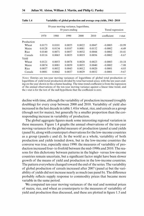
decline with time, although the variability of production increased (roughly doubling) for every crop between 2000 and 2010. Variability of yield also increased in the last decade in table 1.4 for wheat, rice, and cereals as a group (though not for maize), but generally by a smaller proportion than the cor-responding increase in variability of production.

The global aggregate figures mask some interesting regional variation in these measures. Figure 1.4 graphs the annual observations of the ten- year moving variances for the global measure of production (panel a) and yields (panel b), along with counterpart observations for the low- income countries as a group (panels c and d). In the world as a whole, variability of both production and yields trended down, but in the low- income countries the converse was true, especially since 1990: the measures of variability of pro-duction increased four- to fivefold between the mid- 1990s and 2010. The rea-sons for this dichotomy between patterns in the higher- versus low- income countries remain uncertain, but a significant factor might have been slower growth of the means of yield and production in the low- income countries. The pattern everywhere changed toward the end of the series. The variability of global production of cereals increased after 2007 (panel a) but the vari-ability of yields did not increase nearly as much (see panel b). The diVerence probably reflects supply response to commodity prices that became more variable in the same period.

We computed ten- year moving variances of the real and nominal prices of maize, rice, and wheat as counterparts to the measures of variability of yield and production thus discussed, and these are plotted in figure 1.5 and

Table 1.4 Variability of global production and average crop yields, 1961–2010

10- year moving variance, logarithms, 10 years ending Trend regression

1970 1980 1990 2000 2010 coeYcient t- stat

ProductionWheat 0.0173 0.0101 0.0055 0.0022 0.0047 –0.0003 –10.99Maize 0.0128 0.0134 0.0107 0.0081 0.0152 –0.0002 –4.49Rice 0.0140 0.0071 0.0057 0.0032 0.0044 –0.0002 –10.41Cereals 0.0116 0.0065 0.0035 0.0019 0.0056 –0.0002 –8.67

YieldWheat 0.0121 0.0053 0.0078 0.0020 0.0023 –0.0003 –10.18Maize 0.0074 0.0081 0.0059 0.0055 0.0040 –0.0002 –7.08Rice 0.0057 0.0032 0.0043 0.0012 0.0020 –0.0001 –4.03Cereals 0.0081 0.0042 0.0037 0.0029 0.0032 –0.0001 –9.67

Notes: Entries are ten- year moving variances of logarithms of global total production or logarithms of yield (total production divided by total harvested area), with the ten years end-ing on the year shown in the column heading. The time- trend coeYcient is from the regression of the annual observations of the ten- year moving variance against a linear time trend, and the t- stat is for the test of the null hypothesis that the coeYcient is zero.


summarized in table 1.5. As can be seen in figure 1.5, in both nominal and real terms, prices were comparatively stable through the 1950s and 1960s. The pattern changed in the 1970s, reflecting the price spike and its aftermath. Thereafter the patterns for wheat and maize are quite similar but rice is more distinct, with generally higher variability and greater variation in vari-ability over time. Variability of deflated prices was lower in the 1990s than in the 1980s for all three grains but then increased in the early twenty- first century—especially for rice. The changes in price variability—especially in the mid- 1970s and in the mid to late years of the first decade of the twenty- first century—do not appear to be clearly associated with changes in technology; they are more likely linked to other market phenomena that have been widely documented and discussed (see, for example, Wright 2011).

Of course, these prices of grain commodities are diVerent from final con-sumer prices of food that may or may not include grain as an ingredient. Using data from FAO (2013) we computed the country- specific variances of the logarithms of annual average food Consumer Price Indexes (CPI) for the ten- year period of 2001 to 2010 (conceptually comparable to the variances of logarithms of annual average commodity prices in table 1.5, in the column labeled 2010). If we include only the variances for the 172 countries for which we have data for every year, the mean of the logarithmic variances across countries is 0.12, but the median is 0.025 (the distribution

Fig. 1.4 Variability of grain production and yield, ten- year moving variances of logarithms, 1970–2010Note: See table 1.3 and associated text for details.


is very skewed to the left, and for 75 percent of the countries the variance is less than 0.06); this remains true if we exclude a few extreme outliers from either end of the distribution. The corresponding variances of logarithms of international (US) prices of rice, wheat, and maize in table 1.5 are 0.21, 0.09, and 0.10, somewhat larger generally than the counterparts for food CPIs. We would expect domestic prices to be less variable than international prices for grains, depending on country- specific price transmission relation-ships, and we would expect food prices to be less variable than grain prices. Our general observations are consistent with this expectation. However, the variability of CPIs varies tremendously among countries and, while the pat-

Fig. 1.5 Variability of prices of maize, wheat, and rice, 1951–2010Source: These are based on updated versions of prices reported by Alston, Beddow, and Pardey (2009).Note: The ten- year moving variance is plotted against the last year of the corresponding ten- year period, such that a shock in 1971 is reflected in the measures for 1971 through 1980.


terns of variation among the country- specific measures of variability seem generally plausible and consistent with expectations (e.g., very low for Japan and Switzerland), to say anything more specific would require a substantial dedicated research eVort.

1.5 Implications of Alternative Productivity Paths

As discussed above, recent evidence indicates that agricultural productiv-ity growth rates have slowed significantly in many (especially rich) coun-tries over the past twenty years or so (e.g., see Alston, Beddow, and Pardey 2009, 2010; Alston, Babcock, and Pardey 2010), especially in the higher- income countries. In addition, rates of growth in investment in productivity- enhancing agricultural R&D that slowed earlier have turned negative in many (especially high- income) countries, suggesting a worsening of the agri-cultural productivity slowdown in years to come, given the long R&D lags (e.g., see Pardey and Alston 2010; Pardey, Alston, and Chan- Kang 2013). Both the slowdown in agricultural productivity patterns generally and the divergent patterns among countries in rates of research investments and productivity will have implications for future paths of agricultural prices, price variability, and consequences of variability. These outcomes might be moderated by a restoration of research investments and revitalization of

Table 1.5 Variability of prices of rice, maize, and wheat, 1951–2010

Ten- year moving variance of logarithms of prices, 10 years ending

Time- trend coeYcient (t- values in italics)

Crop 1960 1970 1980 1990 2000 2010 1960–2010 1980–2010

A. Nominal valuesRice 0.0061 0.0005 0.0906 0.0620 0.0380 0.2095 0.0019 0.0026

4.22 3.00Wheat 0.0062 0.0327 0.1456 0.0277 0.0386 0.0875 –0.0002 0.0007

–0.23 1.09Maize 0.0302 0.0052 0.1010 0.0409 0.0312 0.1027 0.0003 0.0006

0.61 1.20

B. Deflated valuesRice 0.0082 0.0064 0.0874 0.0664 0.0361 0.0988 0.0015 –0.0013

3.76 –1.48Wheat 0.0111 0.0595 0.0946 0.0328 0.0475 0.0325 –0.0003 –0.0013

–0.88 –3.11Maize 0.0392 0.0063 0.0612 0.0431 0.0409 0.0387 0.0003 –0.0012 1.24 –3.55

Notes: Entries are ten- year moving variances of logarithms of prices, with the ten years ending on the year shown in the column heading. The time- trend coeYcient is from the regression of the annual obser-vations of the ten- year moving variance against a linear time trend, and the t- value is for the test of the null hypothesis that the coeYcient is zero.


productivity growth. To explore these possibilities we conducted simulations using a computable general equilibrium framework.

1.5.1 The Model and the Simulations

Our analysis uses a model and approach developed and applied by Ivanic and Martin (2012) (see also Ivanic and Martin 2008; Ivanic, Martin, and Zaman 2011) to evaluate the impacts of agricultural productivity growth on poverty. Using this model, we extend the analysis of Ivanic and Martin (2012) to evaluate the eVect of agricultural productivity growth on vulner-ability of the poor. To do this we simulate the global economy from 2010 to 2050 under two alternative agricultural technology scenarios: (a) a pes-simistic (slower growth) scenario, with equal productivity growth rates in agriculture and other sectors; and (b) an optimistic (faster growth) scenario, with agricultural productivity growing by one percentage point per year faster than in the rest of the economy. The higher growth scenario involves global average rates of agricultural productivity growth that are broadly in line with the projections of Fuglie (2008). Then, for each scenario we simu-late the eVects of a negative agricultural shock and compare the impacts on the number of people in poverty in a selection of less- developed countries between the optimistic and pessimistic productivity scenarios.

Here we provide a summary description of the key features of the model, which is described in more complete detail by Ivanic and Martin (2012). The simulations were carried out using an aggregated version of the latest Global Trade Analysis Project (GTAP) model that contains the geographi-cal regions defined by the World Bank (East Asia and Pacific, Europe and Central Asia, Developed, Latin America, Sub- Saharan Africa, the Middle East, and South Asia). The thirty- four nonagricultural and nonfood GTAP commodities were aggregated into five categories relevant for this work (agri-cultural farm output, energy, nondurables, durables, and services). The food- related sectors remain disaggregated. Because most of our simulations relate to long- term changes, we applied a long- run closure that allows complete flexibility of employment of capital and labor and limited flexibility of land use. Poverty assessment is based on the household survey data sets collected at the World Bank for twenty- nine developing countries that span the devel-oping world, but notably exclude China. All of the surveys used in this study are relatively recent, and they contain detailed information on the patterns of households’ incomes from and expenditures on agricultural products.21 Behavioral responses of the households in the model are represented using

21. The information on household consumption expenditures, including any own- produced consumption, was separated into seven broad categories: agricultural (food) products, non-durables, energy goods, durables, services, financial expenses, and taxes and remittances paid by the household. The category of agricultural products was further divided into thirty- nine individual commodities, which roughly follow the GTAP commodity classification with some additional crops that may be important to the poor, such as sorghum, cassava, coVee and tea, and potatoes.


expenditure functions to characterize consumption responses, and profit functions to represent output decisions and input responses.22 When prices change, we identify those households whose cost of living less any changes in income moved them across the poverty- line level of utility. We then recal-culate the poverty rate for each country following each simulation and the income and expenditure shares that are the primary determinants of the impacts of price and productivity shocks. Of specific interest is the diVerence in the eVects of a commodity supply shock on poverty outcomes between the optimistic and pessimistic productivity growth scenarios.

1.5.2 The Simulation Results

The baseline projections are intended not as forecasts but as a plausible backdrop against which to examine policy alternatives. These particular results appear to be consistent with the widespread view that substantial growth in agricultural output will be required over the next forty years to meet increasing demand. Under the pessimistic scenario of uniform produc-tivity growth across the agricultural and nonagricultural sectors, the prices of many foods rise substantially: food prices at the household level increase by an average of 48 percent by 2050 (63.3 percent in developing countries). Under the optimistic scenario, with productivity growing 1 percent per year faster in agriculture than in other sectors, food prices rise by a modest 1.4 percent over the same period (8 percent in developing countries).23

Table 1.6 shows the total population in column (1) and the initial base-line percentage poverty rate (at US$1.25 per person per day) in each of the twenty- nine countries of interest in column (2). The next two columns show the eVects of 1 percent higher productivity growth over forty years, 2010 to 2050, in reducing the poverty rate in column (3) and the number of people in poverty in column (4). The new poverty rate under the high- productivity growth scenario is shown in column (5). Thus, for example, in India the initial poverty rate of 43.83 percent applied to a population of 1.17 billion implies a total of some 513 million people in poverty. If global agricultural productivity grew by 1 percent per year faster for forty years, this number would be reduced by 89 million and the poverty rate would be reduced by 7.6 percentage points. The reductions in poverty rates would be even more pronounced in some countries. Across all of the countries in this sample poverty rates would be reduced by an average of 4.75 percentage points and a total of more than 135 million people would be lifted above the poverty

22. The consumer expenditure functions of the households were calibrated to make the elasticities of demand derived from them consistent with those in the macro model. The profit functions were similarly calibrated to ensure that the elasticities of supply that they imply are consistent with those in the macro model.

23. Ivanic and Martin (2012) also examined a scenario with one percent per year higher pro-ductivity in agriculture in developing countries only, under which food prices increase by 13.5 percent (19.2 percent in developing countries). This highlights the importance of productivity growth in developed countries for prices and poverty in less- developed countries as well as showing the central role of productivity growth in less- developed countries.


line under the faster productivity growth scenario. Results such as this are the focus of the study by Ivanic and Martin (2012). Our purpose here is to explore the implications of the same diVerence in baseline productivity growth rates for the vulnerability of people to changes in food markets, as represented by price shocks.

Table 1.7 shows the impacts of a substantial externally generated (say, drought- or crop- pest- induced) price shock on poverty rates under the pes-

Table 1.6 Baseline scenario: Changes in poverty from 1 percent per year higher agricultural productivity growth over 2010–2050

Country Population

(1)

Initial poverty rate, percent

(2)

Change in poverty

New poverty rate, percent

(5)

Percentage points

(3) Headcount

(4)

number percent percent number percentAlbania 3,204,284 0.85 –0.13 –4,104 0.72Armenia 3,092,072 10.63 –1.27 –39,176 9.36Bangladesh 148,692,100 50.47 –4.29 –6,372,561 46.18Belize 344,700 33.50 –1.73 –5,962 31.77Cambodia 14,138,260 40.19 –18.96 –2,680,020 21.23Cote d’Ivoire 19,737,800 23.34 –3.94 –777,204 19.40Ecuador 14,464,740 15.78 –3.27 –473,067 12.51Guatemala 14,388,930 12.65 –5.02 –722,634 7.63India 1,170,938,000 43.83 –7.59 –88,868,501 36.24Indonesia 239,870,900 7.50 –1.54 –3,682,462 5.96Malawi 14,900,840 73.86 –12.71 –1,894,637 61.15Moldova 3,562,062 8.14 –4.04 –143,983 4.10Mongolia 2,756,001 22.38 –6.30 –173,642 16.08Nepal 29,959,360 55.12 –4.46 –1,337,469 50.66Nicaragua 5,788,163 45.10 –5.62 –325,177 39.48Niger 15,511,950 65.88 –2.10 –326,292 63.78Nigeria 158,423,200 64.41 –3.47 –5,493,147 60.94Pakistan 173,593,400 22.59 –6.97 –12,094,064 15.62Panama 3,516,820 9.48 –1.94 –68,181 7.54Peru 29,076,510 7.94 –1.77 –514,516 6.17Rwanda 10,624,010 76.56 –2.26 –239,671 74.30Sri Lanka 20,859,950 14.00 –3.20 –668,386 10.80Tajikistan 6,878,637 21.49 –8.67 –596,488 12.82Tanzania 44,841,220 67.87 –3.62 –1,621,932 64.25Timor- Leste 1,124,355 52.94 –3.29 –37,033 49.65Uganda 33,424,680 51.53 –6.78 –2,267,582 44.75Viet Nam 86,936,460 13.70 –2.10 –1,824,816 11.60Yemen 24,052,510 17.53 –5.25 –1,263,621 12.28Zambia 12,926,410 61.87 –5.30 –684,590 56.58

Notes: In the “low- productivity” scenario, productivity grows at the same rate in agriculture as in the rest of the economy; in the “high- productivity” scenario, productivity grows 1 per-cent per year faster in agriculture than in the rest of the economy in all countries. The changes in poverty in this table reflect 49 percent higher productivity in agriculture as a result of 1 percent higher growth over forty years.

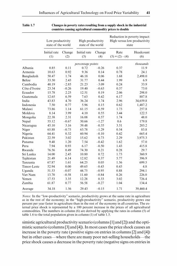
simistic agricultural productivity scenario (columns [1] and [2]) and the opti-mistic scenario (columns [3] and [4]). In most cases the price shock causes an increase in the poverty rate (positive signs on entries in columns [2] and [4]) but in other cases—where there are many poor net- selling households—the price shock causes a decrease in the poverty rate (negative signs on entries in

Table 1.7 Changes in poverty rates resulting from a supply shock in the industrial countries causing agricultural commodity prices to double

Low productivity state of the world

High productivity state of the world

Reduction in poverty impact: High versus low productivity

state

Initial rate

(1) Change

(2) Initial rate

(3) Change

(4) Rate

(5) = (2) – (4) Headcount

(6)

percentage points thousandsAlbania 0.85 0.11 0.72 –0.26 0.37 11.9Armenia 10.63 0.92 9.36 0.14 0.78 24.1Bangladesh 50.47 1.74 46.18 0.06 1.68 2,498.0Belize 33.50 2.43 31.77 0.44 1.99 6.9Cambodia 40.19 –2.85 21.23 –3.09 0.24 33.9Côte d’Ivoire 23.34 –0.26 19.40 –0.63 0.37 73.0Ecuador 15.78 2.25 12.51 0.19 2.06 298.0Guatemala 12.65 6.59 7.63 0.42 6.17 887.8India 43.83 4.70 36.24 1.74 2.96 34,659.8Indonesia 7.50 0.77 5.96 0.15 0.62 1,487.2Malawi 73.86 1.14 61.15 –0.59 1.73 257.8Moldova 8.14 3.99 4.10 0.55 3.44 122.5Mongolia 22.38 2.31 16.08 0.57 1.74 48.0Nepal 55.12 –0.67 50.66 –1.27 0.6 179.8Nicaragua 45.10 3.16 39.48 –0.35 3.51 203.2Niger 65.88 –0.75 63.78 –1.29 0.54 83.8Nigeria 64.41 0.32 60.94 –0.10 0.42 665.4Pakistan 22.59 3.02 15.62 0.73 2.29 3,975.3Panama 9.48 1.20 7.54 –0.42 1.62 57.0Peru 7.94 0.93 6.17 –0.50 1.43 415.8Rwanda 76.56 0.49 74.30 0.21 0.28 29.7Sri Lanka 14.00 2.45 10.80 0.72 1.73 360.9Tajikistan 21.49 6.14 12.82 0.37 5.77 396.9Tanzania 67.87 1.61 64.25 0.05 1.56 699.5Timor- Leste 52.94 0.00 49.65 –0.43 0.43 4.8Uganda 51.53 –0.07 44.75 –0.95 0.88 294.1Viet Nam 13.70 –0.58 11.60 –0.84 0.26 226.0Yemen 17.53 3.35 12.28 0.33 3.02 726.4Zambia 61.87 0.77 56.58 –0.27 1.04 134.4

Average 34.18 1.56 29.43 –0.15 1.71 39,460.4

Notes: In the “low- productivity” scenario, productivity grows at the same rate in agriculture as in the rest of the economy; in the “high- productivity” scenario, productivity grows one percent per year faster in agriculture than in the rest of the economy in all countries. The ex-ternal price shock is represented by a 100 percent increase in the prices of all agricultural commodities. The numbers in column (6) are derived by applying the rates in column (5) of table 1.6 to the total population given in column (1) of table 1.5.



columns [2] and [4]). However, in every case the entry in column (2) is more positive than the entry in column (4), such that the diVerence (in column [5], given by column [2] minus column [4]) is positive—the poverty rate increases by less (from a lower base) or decreases by more in the high- productivity scenario, compared with the low- productivity scenario. This means that the eVect of the price shock on poverty is always more favorable given the high- productivity scenario than the low- productivity scenario. On average across countries in the high- productivity scenario, the external price shock results in a reduction in poverty by 0.15 percentage points, whereas in the low- productivity scenario, the poverty rate increases by 1.56 percentage points. The diVerence reflects a benefit from higher productivity in providing some insulation against the impoverishing eVects of price variability, and—in most cases—reductions in the proportion of the population vulnerable to poverty.

In general, we find that the high- productivity scenario leaves households less vulnerable to price shocks. Higher productivity growth lowers real prices and—given the small price elasticities of demand for staple foods—leaves households with smaller shares of their income spent on food. The high- productivity scenario also leads to a decline in the global share of income from food production given the low price elasticities of demand. For most countries, the reduction in poverty associated with higher productivity reduces the fraction of the population vulnerable to poverty. This is not always the case, however. In countries like Malawi, where the poor fraction of the population was initially more than half, the reduction in the poverty rate may increase the fraction of the population near the poverty line. The numbers are substantial. As shown in column (6) of table 1.7, across the twenty- nine countries, a total of 39.5 million fewer people would be cast into poverty by a doubling of food commodity prices in the high- productivity growth scenario compared with the low- productivity growth scenario. This total benefit—that is, the reduced poverty impact of the price change in the high- productivity growth scenario—reflects the eVects of (a) having a smaller shift of the income distribution induced by the price change in the high- productivity state, and (b) generally having a smaller share of the popu-lation close to the poverty line as illustrated in the heuristic analysis using figures 1.1 and 1.2.

1.6 Conclusion

Technological change in agriculture can aVect the variability of food prices both by changing the sensitivity of aggregate farm supply to external shocks and changing the sensitivity of prices to a given extent of under-lying variability of supply or demand. At the same time, by increasing the general abundance of food and reducing the share of income spent on food, agricultural innovation makes a given extent of price variability less impor-


tant. This chapter has examined these diVerent dimensions of the role of agricultural technology in contributing to or mitigating the consequences of variability in agricultural production, both in the past and looking forward.

A review of patterns of production, yields, and prices for the major cereal grains—wheat, maize, rice, and corn—over the period since World War II indicates that technological change has contributed significantly to growth of yields and production and to reducing real prices, but has probably not contributed to increased price variability. Rather, it seems more likely that technological changes in agriculture may have contributed to an underlying trend of production, yield, and prices that was generally less variable—as measured by moving averages of variances of logarithms of real prices, pro-duction, and yields—with other factors giving rise to periodical increases in variability, such as in the early 1970s and late in the first decade of the twenty- first century. The patterns are not uniform across countries and regions. In particular, production and yields have become more variable in the low- income group of countries during the past decade or so, in contrast to the high- and middle- income groups of countries, with some variation among countries within the groups and across crops. Further work remains to be done to analyze these patterns more formally, and to see whether diVer-ences in agricultural technology, or its location- specific impacts, might have contributed to these seemingly systematic diVerences.

We have emphasized the role of agricultural technology in reducing the importance of food price variability for food security of the poor by reduc-ing the number of farmers, the number of poor, and the importance of food costs in household budgets. An illustrative analysis uses simulations of the global economy to 2050. The results show that the vulnerability of households to poverty is lower following a sustained period of higher pro-ductivity growth.

Appendix A

Prices and Productivity

Between 1975 and 2010, deflated US dollar prices of maize, wheat, and rice fell by about 2.8 percent per year (this is a simple average of the individual rates as reported in the text—see table 1.1), a cumulative decline of about 63 percent of the 1975 prices over the period.24 Over the same interval total global production of cereals (wheat, rice, and coarse grains) grew from about 1,360 million metric tons in 1975 to about 2,430 million metric tons in 2010,

24. The trend growth rate over this period was –2.5 percent per year. Prices fell faster and farther over the interval from 1975 to 2005, after which they increased in real terms.


an increase of about 79 percent relative to 1975 production, and the world’s population increased from about 4 billion to almost 7 billion.

Suppose we assume that the medium- term elasticity of supply of grain is e = 0.5 and the elasticity of demand is η = –0.2. The proportional growth of supply (g) required to achieve a proportional increase in crop output of q = d ln Q (= 79 percent), in spite of a negative proportional change in price of p = d ln P (= –63 percent), is equal to g = q − ep = 79 + (0.5) × 63 = 110.5 percent. Now, let us suppose conservatively, for the sake of argument, that half of the past thirty- five years’ growth in supply is attributable to research- induced productivity improvements (i.e., in round numbers a proportional increase of j = 0.5 such that 100j = 55 percent is half of g = 110 percent growth).

What would the world be like today in the absence of those productivity gains? This can be analyzed by examining the price and quantity eVects of a 100j /(1 + j ) = 35 percent reduction in current supply against the given demand. Given j* = –0.35, e = 0.5 and η = –0.2, the equations for propor-tional changes in price and quantity are p = 100 j*/(e − η) = 50 percent and q = –100 η j/(e − η) = –10 percent. Hence, eliminating thirty- five years of research- induced productivity gains would imply an increase of the cur-rent price of cereals by about 50 percent (19 percent of the 1975 price) and a reduction in the current quantity produced and consumed of about 10 percent (18 percent of the 1975 quantity). These numbers refer to “with” and “without” the research- induced productivity gains. Although they are quantitatively related and of similar orders of magnitudes, they are concep-tually diVerent from the price and quantity changes over time, the “before” and “after” figures, which reflect the eVects of all the variables that changed.

Appendix B

More- Detailed Evidence on Variability of Production and Yield

The following tables report measures of ten- year moving variances of yield and production and regressions of those measures against a time trend, using data for 1961 to 2010.


Table 1B.1 Yields

Average 2010 yield tonnes/ha

10- year moving variance

Time- trend

coeYcient t- stat1970 1980 1990 2000 2010

A. Wheat yieldWorld 3.00 0.0121 0.0053 0.0078 0.0020 0.0023 –0.0003 –10.18

Australia & New Zealand 1.67 0.0290 0.0463 0.0486 0.0328 0.0976 0.0012 3.73

North America 3.02 0.0147 0.0033 0.0063 0.0042 0.0099 0.0000 –1.25Western Europe 6.11 0.0115 0.0084 0.0106 0.0032 0.0036 –0.0003 –6.87China 4.75 0.0615 0.0295 0.0157 0.0067 0.0087 –0.0011 –6.12Asia & Pacific (excl.

China) 2.56 0.0084 0.0099 0.0060 0.0032 0.0013 –0.0003 –15.10Eastern Europe 3.61 0.0231 0.0088 0.0082 0.0059 0.0166 –0.0003 –3.15Latin America 3.33 0.0124 0.0065 0.0100 0.0042 0.0127 –0.0002 –2.16USSR 1.85 0.0488 0.0237 0.0266 0.0113 0.0097 –0.0006 –5.51Northern Africa 2.43 0.0198 0.0094 0.0402 0.0105 0.0103 0.0000 0.12Sub- Saharan Africa 2.05 0.0115 0.0105 0.0212 0.0075 0.0076 –0.0001 –1.46

High income 3.66 0.0080 0.0019 0.0047 0.0021 0.0037 –0.0001 –5.37Upper middle income 2.79 0.0224 0.0108 0.0140 0.0031 0.0041 –0.0004 –9.41Lower middle income 2.70 0.0186 0.0053 0.0088 0.0036 0.0013 –0.0006 –8.31Low income 1.92 0.0065 0.0247 0.0008 0.0044 0.0092 –0.0001 –1.52

B. Maize yieldWorld 5.22 0.0074 0.0081 0.0059 0.0055 0.0040 –0.0002 –7.08

Australia & New Zealand 6.75 0.0197 0.0182 0.0195 0.0069 0.0054 –0.0009 –7.07

North America 9.60 0.0117 0.0118 0.0199 0.0114 0.0051 –0.0002 –2.93Western Europe 9.42 0.0433 0.0099 0.0039 0.0072 0.0039 –0.0007 –6.76China 5.46 0.0359 0.0205 0.0120 0.0037 0.0029 –0.0007 –15.16Asia & Pacific (excl.

China) 3.22 0.0027 0.0046 0.0085 0.0036 0.0130 0.0002 5.43Eastern Europe 5.34 0.0277 0.0111 0.0187 0.0539 0.0396 0.0011 8.18Latin America 4.21 0.0047 0.0058 0.0009 0.0117 0.0095 0.0002 3.60USSR 4.08 0.0294 0.0126 0.0104 0.0170 0.0202 0.0004 3.50Northern Africa 6.10 0.0201 0.0063 0.0169 0.0236 0.0031 0.0001 1.59Sub- Saharan Africa 1.92 0.0102 0.0134 0.0263 0.0226 0.0077 –0.0003 –3.97

High income 9.44 0.0131 0.0102 0.0138 0.0094 0.0044 –0.0002 –5.20Upper middle income 4.92 0.0102 0.0106 0.0021 0.0048 0.0066 –0.0001 –4.28Lower middle income 2.74 0.0027 0.0050 0.0061 0.0117 0.0104 0.0002 8.38Low income 1.70 0.0016 0.0029 0.0021 0.0038 0.0086 0.0000 2.58

(continued )


Table 1B.1 (continued)

Average 2010 yield tonnes/ha


Time- trend

coeYcient t- stat1970 1980 1990 2000 2010

C. Rice yieldWorld 4.37 0.0057 0.0032 0.0043 0.0012 0.0020 –0.0001 –4.03


North America 7.54 0.0088 0.0010 0.0070 0.0016 0.0012 0.0000 0.13Western Europe 6.74 0.0045 0.0128 0.0013 0.0031 0.0005 –0.0002 –4.88China 6.55 0.0234 0.0085 0.0059 0.0020 0.0008 –0.0003 –3.87Asia & Pacific (excl.

China) 3.85 0.0037 0.0031 0.0050 0.0014 0.0029 –0.0001 –2.86Eastern Europe 4.98 0.0089 0.0238 0.0468 0.0280 0.0139 0.0000 0.11Latin America 4.55 0.0015 0.0019 0.0100 0.0143 0.0072 0.0003 6.74USSR 4.30 0.0349 0.0019 0.0015 0.0140 0.0178 0.0002 1.71Northern Africa 9.38 0.0035 0.0022 0.0074 0.0045 0.0008 0.0001 1.64Sub- Saharan Africa 2.15 0.0020 0.0006 0.0040 0.0014 0.0111 0.0001 3.10

High income 6.88 0.0027 0.0042 0.0020 0.0045 0.0009 0.0000 –1.26Upper middle income 5.42 0.0148 0.0044 0.0051 0.0022 0.0010 –0.0002 –3.49Lower middle income 3.83 0.0072 0.0048 0.0081 0.0014 0.0033 –0.0002 –5.44Low income 3.61 0.0017 0.0049 0.0019 0.0037 0.0056 0.0001 4.58

D. Cereals yieldWorld 3.56 0.0081 0.0042 0.0037 0.0029 0.0032 –0.0001 –9.67



China) 3.06 0.0034 0.0048 0.0056 0.0027 0.0032 0.0000 –3.55Eastern Europe 3.78 0.0157 0.0044 0.0027 0.0142 0.0157 0.0001 0.92Latin America 3.97 0.0027 0.0044 0.0008 0.0075 0.0082 0.0001 2.81USSR 1.96 0.0366 0.0215 0.0220 0.0106 0.0081 –0.0004 –5.07Northern Africa 2.77 0.0242 0.0075 0.0241 0.0103 0.0055 0.0000 –0.63Sub- Saharan Africa 1.34 0.0026 0.0073 0.0066 0.0046 0.0044 –0.0001 –5.10

High income 5.32 0.0078 0.0037 0.0054 0.0041 0.0042 –0.0001 –6.46Upper middle income 3.76 0.0182 0.0065 0.0072 0.0041 0.0041 –0.0003 –8.17Lower middle income 2.69 0.0055 0.0054 0.0064 0.0033 0.0032 –0.0001 –7.45Low income 2.07 0.0013 0.0042 0.0003 0.0022 0.0049 0.0000 1.81

Note: Cereals include the following commodities: barley, buckwheat, canary seed, cereal nes, fonio, maize, millet, mixed grain, oats, popcorn, rice, rye, sorghum, triticale, and wheat.


Table 1B.2 Production

2010 production

share


Time- trend

coeYcient t- stat1970 1980 1990 2000 2010

A. Wheat production

World 1.00 0.0173 0.0101 0.0055 0.0022 0.0047 –0.0003 –10.99Australia & New

Zealand 0.03 0.0646 0.0783 0.0573 0.1160 0.1229 0.0013 4.35North America 0.13 0.0159 0.0199 0.0199 0.0020 0.0173 –0.0001 –1.01Western Europe 0.16 0.0120 0.0088 0.0118 0.0065 0.0060 –0.0002 –2.34China 0.18 0.0628 0.0475 0.0218 0.0058 0.0121 –0.0013 –7.22Asia & Pacific (excl.

China) 0.24 0.0239 0.0200 0.0088 0.0043 0.0030 –0.0009 –13.99Eastern Europe 0.05 0.0276 0.0097 0.0186 0.0179 0.0322 0.0002 2.29Latin America 0.05 0.0246 0.0288 0.0139 0.0177 0.0109 –0.0005 –3.20USSR 0.13 0.0510 0.0264 0.0147 0.0241 0.0324 0.0001 0.94Northern Africa 0.02 0.0306 0.0114 0.0474 0.0451 0.0287 0.0010 5.90Sub- Saharan Africa 0.01 0.0422 0.0041 0.0235 0.0145 0.0153 –0.0005 –2.93


B. Maize productionWorld 1.00 0.0128 0.0134 0.0107 0.0081 0.0152 –0.0002 –4.49

Australia & New Zealand 0.00 0.0216 0.0310 0.0232 0.0457 0.0148 –0.0007 –4.26


China) 0.08 0.0127 0.0126 0.0175 0.0050 0.0340 0.0003 2.98Eastern Europe 0.04 0.0225 0.0137 0.0292 0.0448 0.0467 0.0011 7.79Latin America 0.14 0.0243 0.0054 0.0034 0.0108 0.0200 0.0001 1.48USSR 0.02 0.0720 0.0207 0.0327 0.0983 0.1223 0.0039 7.67Northern Africa 0.01 0.0176 0.0113 0.0185 0.0142 0.0065 0.0001 0.75Sub- Saharan Africa 0.07 0.0155 0.0164 0.0476 0.0233 0.0217 –0.0004 –2.59

High income 0.44 0.0146 0.0194 0.0390 0.0192 0.0126 –0.0004 –3.01Upper middle income 0.42 0.0153 0.0136 0.0027 0.0069 0.0182 –0.0001 –1.92Lower middle income 0.09 0.0126 0.0082 0.0325 0.0053 0.0330 0.0003 2.62Low income 0.04 0.0069 0.0081 0.0136 0.0057 0.0220 0.0000 0.94

(continued )


Table 1B.2 (continued)

2010 production

share


Time- trend

coeYcient t- stat1970 1980 1990 2000 2010

C. Rice productionWorld 1.00 0.0140 0.0071 0.0057 0.0032 0.0044 –0.0002 –10.41



China) 0.61 0.0074 0.0082 0.0083 0.0048 0.0056 –0.0001 –4.03Eastern Europe 0.00 0.0435 0.0250 0.0424 0.1513 0.2766 0.0049 2.92Latin America 0.04 0.0156 0.0213 0.0110 0.0123 0.0079 –0.0001 –1.62USSR 0.00 0.3507 0.0362 0.0029 0.0535 0.0487 –0.0038 –4.28Northern Africa 0.01 0.0640 0.0020 0.0120 0.0306 0.0223 0.0003 0.97Sub- Saharan Africa 0.03 0.0159 0.0077 0.0280 0.0041 0.0314 0.0001 0.56


D. Cereals productionWorld 1.00 0.0116 0.0065 0.0035 0.0019 0.0056 –0.0002 –8.67



China) 0.27 0.0076 0.0087 0.0076 0.0034 0.0049 –0.0001 –7.08Eastern Europe 0.04 0.0115 0.0025 0.0030 0.0179 0.0215 0.0003 3.96Latin America 0.08 0.0175 0.0080 0.0015 0.0077 0.0116 –0.0001 –1.95USSR 0.06 0.0316 0.0235 0.0115 0.0461 0.0211 0.0003 1.90Northern Africa 0.01 0.0396 0.0094 0.0289 0.0247 0.0164 0.0002 2.20Sub- Saharan Africa 0.05 0.0075 0.0059 0.0233 0.0087 0.0143 0.0000 0.13


Note: Cereals include the following commodities: barley, buckwheat, canary seed, cereal nes, fonio, maize, millet, mixed grain, oats, popcorn, rice, rye, sorghum, triticale, and wheat.

Fig. 1B.1 Variability of grain production and yield, first differences of logarithm of production, yield and prices

Fig. 1B.1 (cont.)

Fig. 1B.1 (cont.)


References

Alston, J. M., M. A. Andersen, J. S. James, P. G. Pardey. 2010. Persistence Pays: U.S. Agricultural Productivity Growth and the Benefits from Public R&D Spending. New York: Springer Publishers.

Alston, J. M., B. A. Babcock, and P. G. Pardey, eds. 2010. The Shifting Patterns of Agricultural Production and Productivity Worldwide. CARD- MATRIC Electronic Book. May. Ames, IA: Center for Agricultural and Rural Development. http://www.matric.iastate.edu/shifting_patterns/.

Alston, J. M., J. M. Beddow, and P. G. Pardey. 2009. “Agricultural Research, Pro-ductivity, and Food Prices in the Long Run.” Science 325 (4): 1209–10.

———. 2010. “Global Patterns of Crop Yields, Other Partial Productivity Measures, and Prices.” In The Shifting Patterns of Agricultural Production and Productiv-ity Worldwide, edited by J. M. Alston, B. A. Babcock, and P. G. Pardey. CARD- MATRIC Electronic Book. May. Ames, IA: Center for Agricultural and Rural Development. http://www.matric.iastate.edu/shifting_patterns/.

Alston, J. M., R. S. Gray, and K. Bolek. 2012. “Farmer- Funded R&D: Institutional Innovations for Enhancing Agricultural Research Investments.” Canadian Agricul-tural Innovation and Regulation Network Working Paper, University of Saskatch-ewan, Saskatchewan, March. http://www.ag- innovation.usask.ca/cairn _briefs /publications 20 for 20download/CAIRN_2012_FarmerFundedRD_AlstonGray Bolek.pdf.

Anderson, J. R., and P. B. R. Hazell, eds. 1989. Variability in Grain Yields: Impli-cations for Agricultural Research and Policy in Developing Countries. Baltimore: Johns Hopkins University Press (published for the International Food Policy Research Institute).

Beddow, J. M. 2012. “A Bio- Economic Assessment of the Spatial Dynamics of US Corn Production and Yields.” PhD diss. St Paul: University of Minnesota.

Beddow, J. M., P. G. Pardey, B. Koo, and S. Wood. 2010. “The Changing Landscape of Global Agriculture.” In The Shifting Patterns of Agricultural Production and Productivity Worldwide, edited by J. M. Alston, B. A. Babcock, and P. G. Pardey. CARD- MATRIC Electronic Book. May. Ames, IA: Center for Agricultural and Rural Development. http://www.matric.iastate.edu/shifting_patterns/.

Byerlee, D. 2000. “Targeting Poverty Alleviation in Priority Setting for Agricultural Research.” Food Policy 25:429–55.

Cassman, K. G. 1999. “Ecological Intensification of Cereal Production Systems: Yield Potential, Soil Quality, and Precision Agriculture.” Proceedings of the Na-tional Academy of Sciences 96:5952–9.

de Janvry, A., and E. Sadoulet. 2002. “World Poverty and the Role of Agricul-tural Technology: Direct and Indirect EVects.” Journal of Development Studies 38:1–26.

Food and Agriculture Organization of the United Nations (FAO). 2012. FAOSTAT database. Retrieved July 2012 from http:/faostat.fao.org.

———. 2013. FAOSTAT database. Retrieved January 2013 from http:/faostat.fao .org.

Fuglie, K. 2008. “Is a Slowdown in Agricultural Productivity Growth Contributing to the Rise in Agricultural Prices?” Agricultural Economics 39:431–44.

Gardner, B. L. 2002. American Agriculture in the Twentieth Century: How it Flour-ished and What it Cost. Cambridge, MA: Harvard University Press.

Gollin, Douglas. 2006. Impacts of International Research on Intertemporal Yield Sta-bility on Wheat and Maize: An Economic Assessment. Mexico: D.F. CIMMYT.


Hazell, P. B. R. 1989. “Changing Patterns of Variability in World Cereal Produc-tion.” In Variability in Grain Yields: Implications for Agricultural Research and Policy in Developing Countries, edited by J. R. Anderson and P. B. R. Hazell. Bal-timore: Johns Hopkins University Press (published for the International Food Policy Research Institute).

———. 2010. “Asia’s Green Revolution: Past Achievements and Future Challenges.” In Rice in the Global Economy: Strategic Research and Policy Issues for Food Security, edited by S. Pandey, D. Byerlee, D. Dawe, A. Doberman, S. Mohanty, S. Rozelle, and B. Hardy. Los Baños (Philippines): International Rice Research Institute.

Hurley, T. M., P. D. Mitchell, and M. E. Rice. 2004. “Risk and the Value of Bt Corn.” American Journal of Agricultural Economics 86 (2): 345–58.

Ivanic, M., and W. J. Martin. 2008. “Implications of Higher Global Food Prices for Poverty in Low- Income Countries.” Agricultural Economics 39:405–16.

———. 2012. “Agricultural Productivity Growth and Poverty Reduction.” Draft Working Paper, World Bank, Washington, DC, August 6.

Ivanic, M., W. J. Martin, and H. Zaman. 2011. “Estimating the Short- Run Poverty Impacts of the 2010–11 Surge in Food Prices.” Policy Research Working Paper series 5633, World Bank, Washington, DC.

Key, N., and W. McBride. 2007. “The Changing Economics of US Hog Produc-tion.” Economic Research Report no. 52. December. Washington, DC: USDA Economic Research Service.

Lewontin, R. C. 1966. “On the Measurement of Relative Variability.” Systematic Zoology 15 (2): 141–2.

MacDonald, J. M., and W. D. McBride. 2009. “The Transformation of US Livestock Agriculture: Scale, EYciency, and Risks.” Economic Information Bulletin no. 43. January. Washington, DC: USDA Economic Research Service.

Martin, W. J., and J. M. Alston. 1994. “A Dual Approach to Evaluating Research Benefits in the Presence of Trade Distortions.” American Journal of Agricultural Economics 76 (1): 26–35.

———. 1997. “Producer Surplus Without Apology? Evaluating Investments in R&D.” Economic Record 73 (221): 146–58.

Martin, W. J., and K. Anderson. 2012. “Export Restrictions and Price Insulation During Commodity Price Booms.” American Journal of Agricultural Economics 94 (2): 422–7.

Massy, C. 2011. Breaking the Sheep’s Back: The Shocking True Story of the Decline and Fall of the Australian Wool Industry. St. Lucia: University of Queensland Press.

Minot, N. 2011. “Transmission of World Food Price Changes to Markets in Sub- Saharan Africa.” Discussion Paper no. 01059. January. Washington, DC: Inter-national Food Policy Research Institute.

Muth, R. 1964. “The Derived Demand Curve for a Productive Factor and the Indus-try Supply Curve.” Oxford Economic Papers 16:221–34.

Naylor, R., W. Falcon, and E. Zavaleta. 1997. “Variability and Growth in Grain Yields, 1950–94: Does the Record Point to Greater Instability?” Population and Development Review 23 (1): 41–58.

Olmstead, A. L., and P. W. Rhode. 2002. “The Red Queen and the Hard Reds: Pro-ductivity Growth in American Wheat, 1800–1940.” Journal of Economic History 62 (4): 929–66.

———. 2009. Creating Abundance: Biological Innovation and American Agricultural Development. New York: Cambridge University Press.

Pardey, P. G., and J. M. Alston. 2010. US Agricultural Research in a Global Food


Security Setting. A Report of the CSIS Global Food Security Project. Janu-ary. Washington, DC: CSIS. http://csis.org/publication/us- agricultural- research - global- food- security- setting.

Pardey, P. G., J. M. Alston, and C. Chan- Kang. 2013. “Public Agricultural R&D over the Past Half Century: An Emerging New World Order”Agricultural Economics 44, in press, http://onlinelibrary.wiley.com/doi/10.1111/agec.12055/abstract.

Pardey, P. G., J. M. Alston, and V. W. Ruttan. 2010. “The Economics of Innovation and Technical Change in Agriculture.” In Handbook of Economics of Technical Change, edited by B. H. Hall and N. Rosenberg. Amsterdam: Elsevier.

Qaim, M., and D. Zilberman. 2003. “Yield EVects of Genetically Modified Crops in Developing Countries.” Science 299 (5608): 900–2.

Schultz, T. W. 1951. “The Declining Economic Importance of Agricultural Land.” Economic Journal 61 (244): 725–40.

Senauer, B., E. Asp, and J. Kinsey. 1991. Food Trends and the Changing Consumer. St. Paul, MN: Egan Press.

Singh, A. J., and D. Byerlee. 1990. “Relative Variability in Wheat Yields across Coun-tries and Over Time.” Journal of Agricultural Economics 41:2–32.

World Bank. 2012. Food Prices, Nutrition, and the Millennium Development Goals: Global Monitoring Report 2012. Washington, DC: The World Bank.

Wright, B. D. 2011. “The Economics of Grain Price Volatility.” Applied Economics and Public Policy 33 (1): 32–58.

Zilberman, D., and E. Kim. 2011. “The Lessons of Fermentation for the New Bio-economy.” AgBioForum 14 (3): 97–103.

Comment James M. MacDonald

Alston, Martin, and Pardey (AMP) provide a rich and useful framework for thinking about the links among technology, food prices, and the impacts of food price changes on welfare. Innovations in technology work through four channels and can alter:

1. price elasticities of demand and supply for farm commodities, changing the sensitivity of prices to given shifts in supply or demand;

2. the sensitivity of farm supply to external shocks, such as weather or pests, and can therefore influence the degree to which such shocks aVect farm prices;

3. agricultural productivity, and the level of farm prices; and4. economy- wide productivity and real incomes, which leads to falling

shares of income spent on food and hence leaves populations less exposed to food price fluctuations.

James M. MacDonald is chief of the Agricultural Structure and Productivity Branch of the Economic Research Service, US Department of Agriculture.

For acknowledgments, sources of research support, and disclosure of the author’s material financial relationships, if any, please see http://www.nber.org/chapters/c12805.ack.

Documents

The Economics of Food Price Volatility (A National … · This PDF is a selection from a published volume from the National Bureau of Economic Research Volume Title: The Economics