Stanford Undergraduate Economics Journal Spring 2020 Volume 8

Comparative Advantage

Stanford Undergraduate Economics Journal

Spring 2020

Volume 8

Editors and Staff

Editors-in-Chief

Raymond Gilmartin

Matthew Hamilton

Associate Editors

Melda Alaluf

Abeer Dahiya

Tiantian Fang

Matthew Galloway

Avi Gupta

Matin Mirramezani

Sikata Sengupta

Eric Tang

Mary Zhu

Note from the Editors

On behalf of the Comparative Advantage Editorial Board, we are pleased to present the eighth

volume of Stanford University’s undergraduate economics journal.

This year’s journal and blog cover a wide range of topics, such as the effect of monetary policy

announcements on exchange rates, the impact of government investment on education outcomes

in Pakistan, and the potential benefits of a carbon tax. We are grateful to the authors of our

articles, to all who submitted work for consideration, and to our associate editors for their time

and effort during the selection and publication process.

Finally, we would like to thank the Stanford Economics Department and the Stanford Economics

Association (SEA) for their continued support.

Raymond Gilmartin and Matthew Hamilton

2019-20 Editors-in-Chief

Contents

1 The Effect of National Radio on Financial Behavior

Smeet Butala 5

2 The European Central Bank’s Monetary Policy Announcement Effect on theExchange Rate in the Effective Lower Bound Era

Raisa Muhtar 21

3 High Hopes and Low Budget: An Empirical Investigation on the Impact ofDifferential School Investment in Khyber Pakhtunkhwa, Pakistan

Emaan Siddique 34

The Effect of National Radio on Financial Behavior

Smeet ButalaAdvisor: Dr. Peter Murrell

University of Maryland

Abstract— This paper examines the effects of increasingnational coverage of All India Radio on financial inclusionduring the early 2000s. Specifically, the dependent variableis bank account ownership and the explanatory variable ofinterest is subdistrict-level radio coverage. India’s linguisticdiversity means that radio coverage captures the proportionof the population that can effectively listen to accessible radiobroadcasts. I include the standard controls of literacy, wealth,access to banking, and other demographic variables. The rela-tionship between radio coverage and bank account ownershipis regressed using a subdistrict-level fixed-effects model inorder to counteract various endogeneity concerns. Changes inradio coverage are statistically and economically significant, anddemonstrate modest changes in financial inclusion in response.Results vary between rural and urban regions, with ruralregions experiencing greater effects from radio coverage thanurban regions. Several robustness checks confirm the resultsprovided. Policy implications are two-fold: increasing radiocoverage in terms of language and geography across India andincreasing access to radio broadcasts are expected to increasefinancial inclusion.

I. INTRODUCTION

This paper examines the effects of radio coverage onfinancial inclusion. Specifically, it explores the link betweenAll India Radio’s broadcast coverage across India and Indianbank account ownership using data from the two census yearsof 2001 and 2011.

In this analysis, I examine how changes in radio coverageof All India Radio (AIR), or Akashvani, affect subdistrict-level financial inclusion. I construct various measures ofradio coverage in order to generate composite measures oflistenership that form the core independent variables. Ascontrols, I include principal determinants of financial inclu-sion relevant at the subdistrict (tehsil) level, such as literacy,access to banks, wealth, and a number of demographicvariables. I estimate this relationship using subdistrict fixed-effects and by clustering standard errors over subdistricts.The data for these variables is obtained from All India Radio,Prasar Bharati, and the 2001 and 2011 Censuses of India.

Financial inclusion, defined as the availability of and un-encumbered access to financial services, is generally thoughtto have significant beneficial long-term impacts on poverty(Beck, Demirguc-Kunt, and Martinez Peria, 2007; Beck,Demirguc-Kunt, and Levine, 2007; Clarke, Xu, and Zou,2006; Galor and Zeira, 1993; Honohan, 2004; Jeanneney andKpodar, 2011). Financial inclusion, and particularly access tobanking, is regarded as a major potential social safety net formuch of the world’s poor. Owning a bank account, generally

a transaction account, promotes financial planning and otheraspects of financial safety, but also promotes the use of otherfinancial services, such as credit and insurance (Carbo et al.,2005; Leyshon and Thrift, 1995; Mohan, 2006, RangarajanCommittee, 2008).

In the Indian context, the concept of financial inclusiongained prominence with the Reserve Bank of India’s 2005Annual Policy Statement by then-governor Dr. VenugopalReddy (Reddy, 2006). Following that, the Rangarajan Com-mittee in 2008 placed much greater emphasis on the im-portance and need for financial inclusion, calling it “botha crucial link and a substantial first step towards achievinginclusive growth” (Rangarajan Committee, 2008). Both ofthese represent government-directed efforts at not only pop-ularizing and promulgating the concept, but at promotingan academic interest in it as well. However, it should beunderstood that India’s policy of providing accessible bank-ing throughout the country stretches much further back, mostnotably with the Regional Rural Bank program. The programwas well-regarded for greatly expanding rural banking, andhas been shown to have had noticeable effects on ruralpoverty reduction in India (Burgess and Pande, 2005).

All India Radio (AIR), also known as Akashvani, is India’snational public radio broadcaster. AIR began in 1936 inKolkata, and, as of 2011, reached over 98% of India’spopulation. Despite this, from 2001 to 2011, AIR added34 new stations across the country, an expansion of about17%. A number of these new stations also increased thelanguages they broadcast in, seeking to engage more withunderserved and historically overlooked communities. AIRoperates under a three-tier system — national, state, andlocal — in which stations broadcast programming and newsbulletins from each of the three tiers. The national tierbroadcasts in Hindi and English, the state tiers broadcastin official state languages, and the local tiers broadcast inlocally prominent languages. The national and state tiersbroadcast both news bulletins and other programming in allof their respective languages, whereas the local tier is givenautonomy in deciding the extent to which its languages areto be used. Thus, of the local tier languages, some may beused for news bulletins and programming, whereas some mayonly be used for specific programming.

All India Radio broadcasts a variety of programs, fromentertainment to education to programs specifically for atarget audience, such as farmers, women, and youth. Many ofthese programs include financial education, financial advice,

5

or other pieces of financial information. Particularly, thereare a variety of business or financial programs covering anarray of financial education topics. Additionally, there areprograms for farmers focusing on interest rates, insurancepolicies, and loans, and programs for women focusing onfinancial independence, among many more. All in all, amultitude of groups are informed on a variety of financialtopics, most of which are centered around the opening anduse of a bank account.

My core results show that there are indeed tangible effectsto increasing AIR coverage in India. The findings show that,as a whole, India experiences a significant rise in bank ac-count ownership from increases in radio coverage, implyingthat AIR-based financial education is successful at changingthe financial behavior of many of its listeners. Observingthe rural-urban divide, rural regions experience a high rateof financial participation as compared with urban regions.This suggests that, despite equivalent increases in coveragein urban regions, there are urban-specific factors that preventfinancial education from translating to financial inclusion.Generally, urban residents are noted to be more multilingualthan rural residents. Thus, an increase in coverage in theirnative language may be less effective than it would be forrural residents, for whom increases in language coverageare much more critical. Further, urban residents are moreexposed to banks and to banking than rural residents are,for whom such radio broadcasts can be highly informative.Additionally, the results for both rural and urban regionsshow that bank account ownership is only increasing in radiocoverage if there is sufficient radio ownership in the givensubdistrict. Otherwise, broadcasts do not seem to reach theintended audience.

My results present clear policy implications for AIR andPrasar Bharati, its parent organization. Primarily, expandingAIR coverage across India, geographically and linguistically,has much potential to further government initiatives forfinancial inclusion. Considering AIR’s present geographicalreach, increases in coverage are more likely to come in theform of expanding the number of languages broadcast at astation. Thus, with increased language diversity across AIRstations, there can be increased information disseminationand penetration to many presently unreached populations.In addition to this, however, AIR must ensure high enoughrates of radio access, through radio sets, for the increases inbroadcast coverage to be effective.

The paper is organized as follows. Section II provides areview of the literature regarding banking and broadcasting inIndia. Section III describes the data and variables. SectionIV presents the results from the main regressions. SectionV examines several robustness checks of the core results.Section VI presents the conclusions.

II. LITERATURE REVIEW

Financial inclusion has been a major development goalfor both developed and developing nations since the early2000s, at the national and sub-national level. Additionally,

it has been a major focus for several multinational organi-zations. The general meaning of financial inclusion is theavailability and access of financial services to all individualsin the economy. Often, this occurs through the expansionof bank branches and the development of more coherentpolicies aimed at the disenfranchised and disadvantaged(Carbo et al., 2005; Clarke, Xu, and Zou, 2006; Conroy,2005; Beck, Demirguc-Kunt, and Levine, 2007; Honohan,2004; Leyshon and Thrift, 1995; Mohan, 2006; RangarajanCommittee, 2008). Financial inclusion generally begins withaccess to banking services, with access to credit consideredan important secondary step. This paper will focus on thefirst of these, on the effect of financial education on banking,although it is well documented that the first generally leadsto the second (Allen et al., 2012; Bhandari, 2009; Sarap,1990).

It is well-documented in the development literature that ac-cess to and ownership of a bank account enables householdsto engage in significant levels of consumption smoothingover time; this has also been suggested to reduce the inci-dence of child-labor among these households (Becker, 1975;Blundell et al., 2017; Mincer, 1974). The literature also linksbanking to savings mobilization and access to credit. Theseare associated with greater capital accumulation, longer-term investment decisions, and significant poverty reduction(Burgess and Pande, 2005). Further, a number of papersdemonstrate that poverty and inequality are negatively asso-ciated with access to formal financial services (Clarke, Xu,and Zou, 2006; Beck, Demirguc-Kunt, and Martinez Peria,2007; Honohan, 2004; Galor and Zeira, 1993; Jeanneney andKpodar, 2011). Moreover, much of the literature notes thatgreater access to financial services has significant positive ex-ternalities, improving a variety of measures of economic ef-ficiency, equity, financial development, and economic growth(Abu-Bader and Abu-Qarn, 2008; Bittencourt, 2012; Conroy,2005; Pal, 2011; Yang and Yi, 2008).

Financial literacy is generally regarded as a criticalstepping-stone towards financial inclusion, as it educatesindividuals on the range of financial products they mayobtain. However, several studies demonstrate that India,like much of the world, has very low levels of financialliteracy across all population groups (Agarwal et al., 2015;Bonte and Filipiak, 2012; Huston, 2010). There are severalstudies conducted in India and similar developing nationsthat demonstrate the effect of financial literacy on financialbehavior. The majority of such papers show limited effectsof financial literacy programs on those already financiallyliterate, but that there are modest inclusion improvementson the financially illiterate (Atkinson and Messy, 2011; Coleet al., 2009; Miller et al., 2009). Additionally, these resultsdepend on the population to whom financial education isprovided, with different groups responding differently dueto any number of population-specific factors (Arora, 2016;Dixit and Ghosh, 2013; Gaurav and Singh, 2012; Nedungadiet al., 2018).

Regarding the link between radio and the dissemination offinancial information, very little research has been conducted,

6

TABLE I: Method 1 and Method 2 for Representing Language Coverage (LCV)

Method Value AssignedLanguage Coverage no coverage non-news coverage news coverageMethod 1 (LCV1) 0 1Method 2 (LCV2) 0 1

particularly in India. One of the most prominent studies,however, documents that regular radio and television usehas meaningful impacts on the awareness and understandingof various financial instruments, though it does not showan increase in investment in these instruments (Bonte andFilipiak, 2012). Additionally, numerous papers demonstratethe usefulness of radio for information dissemination in Indiaand similar developing nations in the fields of health andtechnology (Sharma and Choudhary, 2007; Annamalai, 2001;Kakade, 2013; Nazam, 2000; Opara, 2008; Tamuli, 1999).

Radio-based financial education is ubiquitous in India,yet there is a dearth of research examining this medium ofeducation and its effects on financial inclusion. This paperseeks to address this gap in the literature by presenting ananalysis on All India Radio, arguably India’s most well-known and most listened-to radio service, and whether AIRhas been successful in improving India’s levels of financialinclusion.

III. DATA AND METHODS

Using All India Radio and Prasar Bharati, I compile anoriginal panel of station-level data on subdistricts coveredand broadcasting languages, primarily for the purpose ofconstructing the main variable of interest, Effective Reach.India is a notably diverse nation linguistically. A region’sofficial languages, Hindi, and the state language(s) may notbe well-understood by the many segments of the population.This can significantly lessen the effect of radio broadcastsintended to educate the public. Thus, it is possible thatsignificant portions of certain subdistricts might be unableto speak any of the languages broadcast in their region. Inlight of these circumstances, I construct a variable, EffectiveReach (ER), that seeks to capture the population for whomthe available AIR broadcasts are understandable, the effectivepopulation reached. Essentially, I intend to summarize howwell a subdistrict is “matched” by the broadcasts it receives;subdistricts with a high linguistic match will return a highvalue for ER, and subdistricts that receive broadcasts thatdo not match their linguistic demography will return a lowvalue for ER. It is constructed as follows:

ERi =∑

l

MTil ∗maxs

(LCVils) (1)

where MT is Mother Tongue (over population) and LCVis language coverage for subdistrict i, language l, and AIRstation s.

Specifically, MTil is the proportion of individuals insubdistrict i for whom language l is the mother tongue.Mother Tongue is used in the absence of a variable recordingspeakers by language at the subdistrict level. The primaryassumption mitigating concerns of measurement error is that

listeners will prefer their first language, and would thuschoose to listen primarily, or only, to radio broadcasts inthat language. LCV ils records the coverage by station s oflanguage l in subdistrict i. Language coverage attempts toassign a value to the broadcasting languages at a station.Unfortunately, a nontrivial number of stations provide onlyvery limited information about their broadcasts, and thus Ihave elected to use a station’s news-bulletin in generatingthese values. I classify languages based on whether theyare used to relay news-bulletins, whether they are usedfor strictly non-news broadcasting, or whether they are notpresent at the station.

I devise two methods of interpreting the language coverageclassification by generating two separate dummy variables,presented in Table I. Under the first, referred to as method 1,I construct LCV 1, a dummy variable defined as 1 if, in sub-district i, station s uses language l for news-bulletin broad-casting. The assumption underpinning the use of method 1is that, for listeners of a specific language, coverage belownews-level coverage is insufficient for influencing financialbehavior. The alternative method to this is referred to asmethod 2. Under this method, I construct LCV 2, a dummyvariable defined as 1 if, in subdistrict i, station s useslanguage l for any amount of broadcasting. The assumptionunderpinning the use of method 2 is that any coverage issufficient for influencing financial behavior. Thus, I generatetwo alternative measures of Effective Reach: ER1 and ER2.

The remainder of the data is obtained directly from theCensus of India, years 2001 and 2011. Earlier censusescontain were not used because they did not record householdbanking data. From the data, I am able to make use of threedifferent sets of observations. The first set includes data onwhole subdistricts (10,873 observations), henceforth referredto as total. The second set includes data on the rural portionsof subdistricts (10,785 observations, as not all subdistrictshave rural parts), henceforth referred to as rural. The thirdset includes data on the urban portions of subdistricts (5,551observations, as many subdistricts do not have urban parts),henceforth referred to as urban. Summary statistics can befound in Appendix A, Tables 1 and 2.

The dependent variable in my analysis is Bank AccountOwnership (BO), which represents the proportion of house-holds in a subdistrict that are in possession of a bank account.This records households in possession of one account asequivalent to households where multiple adults possess theirown, independent accounts. In order to capture the proportionof the population that has access to radio broadcasts, Iconstruct both Radio Ownership (RO) and Car Ownership(CO). Radio Ownership is defined as the proportion ofhouseholds in a subdistrict that are in possession of a radioset or a transistor radio. Additionally, as cars and other auto-

7

mobiles are generally outfitted with a radio console, I includeCar Ownership, defined as the proportion of households ina subdistrict that are in possession of a car, van, or jeep.

Effective Reach captures the maximum potential reach thatAIR broadcasts can have in a subdistrict. However, low ratesof radio access would render Effective Reach values partic-ularly meaningless. As such, in order to capture effectivelistenership, I make use of two interaction terms: ROxERand COxER. ROxER captures the radio set/transistorradio-based effective listenership, where COxER capturesthe automobile-based effective listenership. In addition tothese variables, I include a number of control variablesthat are determinants of financial inclusion seen as standardin the literature, namely wealth, literacy, access to finan-cial institutions, and country-specific demographic variables(Bhattacharyay, 2016; Khanh, et al., 2019; Kumar, 2013;Sahoo et al., 2017; Singh et al., 2017).

Following the work of Filmer and Pritchett (2001),McKenzie (2005), Vyas and Kumaranayake (2006), andseveral others, I construct an asset-based wealth index bymeans of principal component analysis. The majority of suchindices are constructed for the purpose of scoring and rankinghouseholds by wealth; however, in my analysis, I turn fromscoring households to scoring subdistricts. The Census ofIndia provides an abundance of household and housing data,and I am able to collect 81 assets for 2001 and 119 assets for2011. This data is provided, in line with the other variables,as the proportion of households in a subdistrict that have orhave access to a given characteristic/asset. Essentially, thisasset index scores a subdistrict’s wealth in accordance withthe wealth of the households comprising that subdistrict.

Concerns over the inclusion of irrelevant assets or char-acteristics in the index are generally unfounded. Includedvariables fall under one of the following categories, each ofwhich is an indicator of household wealth: housing condition,house-ownership status, housing materials, number of rooms,household member characteristics, water and water access,electricity and fuel, latrine and bathing room facilities,kitchen facilities, and assets.

From this, the final variable, Wealth Index is constructedby weighting each of the included variables for each subdis-trict, resulting in a singular, summarized value that indicatesthe subdistrict’s wealth relative to the other subdistricts inthe country. As is usual in the literature, I standardize (mean-center and divide by the standard deviation) this measure bypopulation set (total/rural/urban) and by year in order to fa-cilitate interpretation of its estimated coefficients (Filmer andPritchett, 2001; McKenzie, 2005; Vyas and Kumaranayake,2016).

Literacy, among a variety of education variables, is gen-erally strongly associated with financial participation in theliterature. As such, I include Literacy Rate, which measuresthe proportion of the population that is literate by subdistrict.Access to financial institutions and banking facilities isanother important determinant of financial inclusion. TheCensus of India provides information on the number of banksper capita present within a subdistrict. From this, I generate

two variables: sdBI and dBI . sdBI is the number of banksin the given subdistrict. However, individuals living in asubdistrict are not confined to banking solely within theirsubdistrict. In order to account for this, I construct dBI , thenumber of banks in a given district per capita (of the district).Together, these two variables seek to capture banking access.

Finally, I include a number of demographic variables toaccount for demographic-specific barriers or advantages tofinancial inclusion. The Census of India provides the genderratio as well as the proportion of religious minorities (Mus-lim, Christian, Sikh, Buddhist, Jain, Other) per subdistrict,and thus I include each of these in my analysis.

Additionally, in order to correct for subdistrict-specificendogenous characteristics that cannot be accounted for –cultural or social drivers, or that lack sufficient data –spending on financial infrastructure, education, or radio,I implement subdistrict fixed-effects. Further, I cluster onsubdistricts in order to produce cluster-robust standard errors.Using these variables, I estimate the following two empiricalmodels that differ only in their use of ER1 or ER2:

BOit =α+ β1ROit + β2COit + β3ER1it+ β4ROit ∗ ER1it + β5COit ∗ ER1it + β6Litit

+ β7sdBIit + β8dBIit + β9WIit +ZZZ ∗ γγγ+ θt + φi + εit; t = 0, 1; i = 0, ..., N (2)

BOit =α+ β1ROit + β2COit + β3ER2it+ β4ROit ∗ ER2it + β5COit ∗ ER2it + β6Litit

+ β7sdBIit + β8dBIit + β9WIit +ZZZ ∗ γγγ+ θt + φi + εit; t = 0, 1; i = 0, ..., N (3)

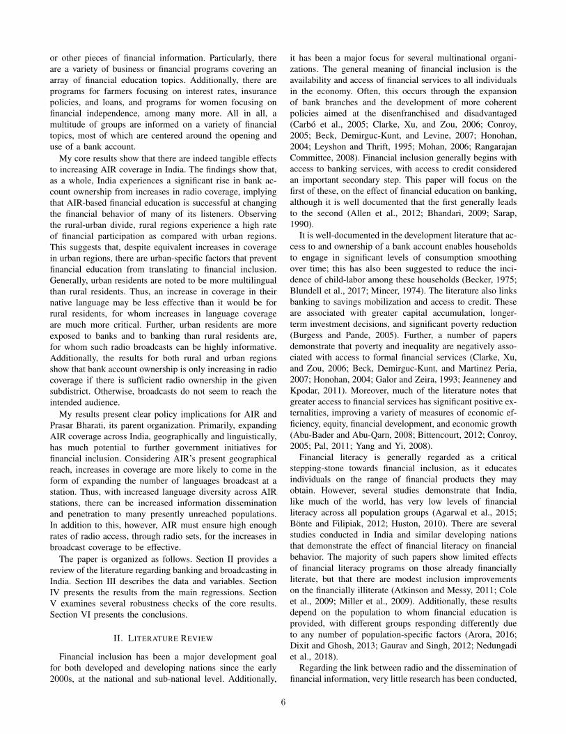
for subdistrict i and time period t. The term ZZZ is a vectorof control variables, γγγ is the vector of their coefficients, θt isthe set of time fixed-effects, and φi is the subdistrict-specificfixed-effects term. A description of all variables can be foundin Table IV.

IV. RESULTS

Table V presents estimates of the model as specifiedabove, where the first three columns are estimates of equation(2) and the second three columns are estimates of equation(3).

A. Effective Reach

The variable of interest, Effective Reach, is interpretedthrough an examination of the marginal effects. From hereone, when I refer to estimates, I will be referring to estimatesof marginal effects.

∂BO

∂ER= β3 + β4 ∗ROit + β5 ∗ COit (4)

Estimates of Effective Reach vary depending on the popula-tion set used. Estimates are increasing in Radio Ownershipand Car Ownership under total and rural; however, interest-ingly, estimates are decreasing in either Radio Ownership,

8

Car Ownership, or both, under urban. increasing in CarOwnership about two (method 1) to three (method 2) timesthe rate of increases in Radio Ownership. This suggests thatradio access by means of Car Ownership has a noticeablylarger impact on Bank Account Ownership than does radioaccess by means of Radio Ownership. This is discussedfurther under Car Ownership. Despite being increasing inthese two variables, the majority of subdistricts do not actu-ally experience increases in Bank Account Ownership fromincreases in Effective Reach. Rather, only 25.44% (method1) to 46.18% (method 2) of subdistricts have Radio and CarOwnership levels sufficient for increases in Effective Reachto translate to increases in Bank Account Ownership. Further,the average marginal effect (of the positive values) presentsonly modest values, 0.037 (method 1) or 0.043 (method2). This implies that a 1% increase in in Effective Reach,essentially a a 1% increase in the broadcasting-linguisticmatch, leads to a 0.037%-0.043% increase in Bank AccountOwnership. Put in other terms, in a subdistrict of population10,000, radio service for 100 more people results in 3-4additional individuals obtaining a bank account. Moreover,some subdistricts experience rather high marginal effects; thetop 1.83% (method 1) and 4.04% (method 2) of subdistrictsexperience marginal effects of 0.1 or higher, or a 0.1%increase in Banking from a 1% increase in Effective Reach.

Using rural population, we obtain rather similar results.Again, only 25.03% (method 1) to 49.32% (method 2) ofsubdistricts have Radio and Car Ownership levels sufficientfor increases in Effective Reach to have positive effects onBank Account Ownership. And, the average marginal effect(of positive values) is slightly lower, at 0.032 (method 1) or0.037 (method 2), implying that a 1% increase in EffectiveReach leads to a 0.032%-0.037% increase in Bank AccountOwnership. Despite this, the top 1.01% (method 1) and thetop 2.56% (method 2) of subdistricts experience marginaleffects of 0.1 or higher, or a 0.1% increase in Banking froma 1% increase in Effective Reach. Essentially, estimates usingboth total and rural populations suggest that high levels ofRadio and/or Car Ownership are required for increases inEffective Reach to have economically significant effects onfinancial participation.

Under urban populations, estimates using ER1 are quitedifferent from estimates using ER2. Method 1 estimates ofER1, RO×ER1, and CO×ER2 are statistically insignifi-cant, as are the resultant marginal effects, implying negligibleeffects from changes in ER1. Examining estimates usingmethod 2, 48.00% of subdistricts have Radio and Car Own-ership levels sufficient for ER2 to have positive effects onBank Account Ownership. Additionally, the average marginaleffect (of positive values) is much lower, at 0.021, implyingthat a 1% increase in ER2 leads to a 0.021% increase inBank Account Ownership. Changes in All India Radio urbancoverage have much smaller effects than changes in ruralcoverage.

B. Radio Ownership

Interpretation of the estimates of Radio Ownership alsorequires an examination of the marginal effects.

∂BO

∂RO= β1 + β4 ∗ ERit (5)

Estimates of Radio Ownership, using total populations,is increasing in Effective Reach. Marginal effects at themean (ER1 = 0.515, ER2 = 0.572) are negative at -0.0144 (method 1) and -0.0264 (method 2). However, atER1=0.568 and ER2 = 0.673, the marginal effects of RadioOwnership become positive. Accordingly, we see that only53.32% (method 1) to 50.89% (method 2) of subdistrictshave Effective Reach at sufficiently high levels for increasesin Radio Ownership to result in positive changes in BankAccount Ownership. Similarly, using rural populations, wesee that estimates of Radio Ownership are increasing inEffective Reach. Marginal effects at the mean (ER1 = 0.527,ER2 = 0.588) are negative at -0.0279 (method 1) and-0.0417 (method 2). And, in line with the total results,we see that only 52.11% (method 1) to 48.05% (method2) of subdistricts have Effective Reach at sufficiently highlevels for increases in Radio Ownership to result in positivechanges in Bank Account Ownership. However, under urbanpopulations, estimates of Radio Ownership are decreasing inEffective Reach, but are positive across all values of ER.Marginal effects at the mean are much higher as well, at0.1233 (method 1) and 0.1308 (method 2), implying that a1% increase in Radio Ownership translates to a 0.1233% or0.1308% increase in Bank Account Ownership.

C. Car Ownership

Interpretation of the estimates of Car Ownership alsorequires an examination of the marginal effects.

∂BO

∂CO= β2 + β5 ∗ ERit (6)

Estimates of Car Ownership using total populations, areincreasing in Effective Reach. Marginal effects at the mean(ER1 = 0.515, ER2 = 0.572) are positive at 0.1886(method 1) and 0.1944 (method 2), implying 0.1886% and0.1994% changes in Bank Account Ownership from percentunit changes in Car Ownership. The majority of subdistrictssee positive marginal effects of Car Ownership: 67.51%(method 1) and 71.45% (method 2) of subdistricts. Estimatesusing rural populations present more positive effects fromincreases in Car Ownership. Marginal effects at the mean(ER1 = 0.527, ER2 = 0.588) are slightly lower, however,at 0.1496 (method 1) and 0.1911 (method 2). But notably,100% of subdistricts under method 1 specifications havepositive marginal effects of Car Ownership, whereas 78.60%of subdistricts under method 2 specifications have positivemarginal effects. Finally, estimates using urban populationsare similar to rural estimates. Marginal effects at the mean(ER1 = 0.515, ER2 = 0.552) are positive, at 0.1823(method 1) and 0.1317 (method 2), and again, 100% ofsubdistricts (method 1) and 75.58% of subdistricts (method 2)

9

have positive marginal effects of Car Ownership. However, itshould be noted that, for urban populations under method 2specifications, the marginal effects are decreasing in EffectiveReach.

A point of concern with the above estimates is thatCar Ownership appears to be proxying wealth, producinga potential upward bias in the estimates. As such, I providea robustness test without Car Ownership in Section V todemonstrate that this behavior is inconsequential.

D. Literacy Rate

The coefficients on Literacy Rate are economically andstatistically significant for total and rural populations. Wesee rather high levels of impact from increasing the LiteracyRate, with a 1% increase resulting in a 0.202% to a 0.251%increase in Bank Account Ownership, consistent with theliterature (Khanh, et al., 2019; Kumar, 2013; Sahoo et al.,2017; Singh et al., 2017) about the impact of education onfinancial inclusion. However, what is unusual is the estimatesfor urban populations. These coefficients are not statisticallysignificant and are only weakly economically significant.Further, the coefficients are negative, implying decreasesto Bank Account Ownership from increases in the LiteracyRate. These findings agree with some of the literature aboutIndia’s urban poor, which note that literacy or education areoften insufficient to overcome barriers to financial inclusion(Chakrabarti and Sanyal, 2016; Rajeev and Vani, 2017).

E. Wealth Index

The coefficients on the Wealth Index are economicallyand statistically significant for all population sets. Estimatesusing total populations are of a moderate level, at around0.09. Estimates using rural populations are slightly lower,at around 0.064, and estimates using urban populationsare about 55% higher than rural estimates, at around 0.1.The Wealth Index has been standardized (mean-centered anddivided by the standard deviation). Thus, the above estimatescan be interpreted as: a 1 standard deviation increase inwealth corresponds to a 9% (total), 6.4% (rural), or 10% (ur-ban) increase in Bank Account Ownership. These coefficientsare generally consistent with the literature (Bhattacharyay,2016; Khanh, et al., 2019; Kumar, 2013; Sahoo et al., 2017;Singh et al., 2017) about the impact of wealth on financialinclusion, and suggest wealth is more significant a factor inurban regions than in rural regions.

F. Banking Institutions

Interpretation of the estimates of Banking Institutions doesnot immediately suggest marginal effect analysis. However,by construction of dBI , we have:

dBIi =

∑di (Banksi)∑d

i (Populationi)

and sdBIi =Banksi

Populationi

Thus, we have

dBIi =Banks1 +Banks2 + ...+Banksd∑d

i (Populationi)

dBIi =Banksi∑d

i (Populationi)

+Banks1 + ...+Banksi−1∑d

i (Populationi)

+Banksi+1 + ...+Banksd∑d

i (Populationi)

dBIi =sdBIi ∗ Populationi∑d

i (Populationi)

+Banks1 + ...+Banksi−1∑d

i (Populationi)

+Banksi+1 + ...+Banksd∑d

i (Populationi)

and, therefore, from equations (2) and (3)

∂BOi

∂sdBIi= β7 + β8 ∗

Populationi∑di (Populationi)

Thus, we see that the marginal effects of Banking Institu-tions, as specified in these models, are dependent on relativesize of the subdistrict’s population to its district’s population.For total populations, it appears that the vast majority ofsubdistricts experience increases to Bank Account Ownershipfrom increases in the number of banks present; 100% ofsubdistricts under method 1 have positive marginal effects,and, under method 2, subdistricts whose populations aregreater than 0.021% of their district’s population have posi-tive marginal effects. This amounts to 99.32% of subdistricts.Interestingly, however, the estimates presented using ruraland urban populations are strikingly contrary to the totalpopulation estimates. Marginal effects for rural and urbanpopulation sets are decreasing in relative population size, andthe marginal effects become negative after surpassing ratherlow thresholds: from 0.339% to 0.527% of their district’spopulation. As such, the vast majority of subdistricts, underrural and urban, experience negative marginal effects ofBanking Institutions on Bank Account Ownership.

V. ROBUSTNESS

In this section, I examine the robustness of the core esti-mates. Primary concerns regarding the estimates of equations(2) and (3) include potential endogeneity or feedback fromcertain regressors and the arbitrariness of controls included.I present estimates of alternate models in order to argue thatthe problems associated with these issues are not important.

The assumption that household wealth strongly influencesa household’s financial participation status is common in theliterature (Khanh, et al., 2019; Kumar, 2013; Sahoo et al.,2017; Singh et al., 2017). However, it is highly plausibleto consider that financial inclusion may have positive im-pacts on long-term household wealth. Thus, to maintain the

10

consistency of the estimates presented earlier, wealth levelsmust be strictly exogenous from levels of financial inclusion,as would be expected from a lagged effect. In Table VI, Ipresent estimates of equations (2) and (3) omitting the wealthindex. The core estimates of ER, RO, and their interactionsare largely similar to those from Table V, whereas estimatesof CO and CO × ER are somewhat lower and have lessstatistical significance.

As mentioned in the discussion of the estimates for CarOwnership, the estimates suggest that Car Ownership couldbe serving as a proxy for wealth in the regression. Owning acar is not ubiquitous in India, with data from 2011 showingthat only 2.8% of households owned a car (with bicycleand motorcycle ownership much higher). Thus, higher ratesof Car Ownership may be producing higher estimates notbecause car-based radio access is more effective at conveyingfinancial information, but because the estimates appear to beproxying the subdistrict’s wealth. As such, in Table V II ,I present estimates of equations (2) and (3) omitting CarOwnership and its interaction term CO × ER. The coreestimates of ER, RO, and their interactions are broadlysimilar to those from Table V, clearly demonstrating theirrobustness.

Another assumption found frequently in the literature isthat (Bhattacharyay, 2016; Khanh, et al., 2019; Sahoo et al.,2017; Singh et al., 2017) access to banking is a determinantof financial inclusion. However, it is not implausible toconsider that higher levels of financial inclusion could act asa determinant of banking access. As noted above, to maintainthe consistency of the previously presented estimates, accessto banking must be strictly exogenous from levels of financialinclusion. In Table VIII, I present estimates of equations (2)and (3) omitting both banking variables, sdBI and dBI .Here I note that the core estimates of ER, RO, CO, andtheir interactions are largely similar to those from Table V.

A final concern is related to the demographic variablesincluded. The choice of variables included may be seen asarbitrary, and other variables which were not available inthe data may seem more relevant. In Table IX , I presentestimates of equations (2) and (3) omitting the demographicvariables. I observe that the core estimates of ER,RO,CO,and their interactions are largely similar to those from TableV.

VI. CONCLUSION

The results reflect the different characteristics of rural andurban regions. From 2001 to 2011, there was a marked risein bank account ownership throughout India. However, theseincreases were not homogeneous; the average bankednessin rural regions rose 23.93 percentage points to 52.26%,whereas for urban regions it rose by only 16.54 percentagepoints to 62.74%. At mean values of Radio Ownership andCar Ownership, we see that subdistricts experience onlyweak gains, and even losses, from increases in EffectiveReach. However, at high levels of RO and CO, EffectiveReach has a much stronger effect on Bank Account Own-ership.

Comparing rural and urban regions, increases in EffectiveReach (increases in the broadcasting-linguistic match) havestronger impacts in rural India at all levels of RO and COas compared with urban India. There are several potentialexplanatory circumstances affecting this. Primarily, urbanregions in India are widely recorded to have higher ratesof multilingualism, which is not captured by Mother Tongue.This reduces the impact of increasing AIR language coveragein these urban regions, as higher percentages of urban lin-guistic minorities will already be in AIR’s reach as comparedwith rural regions. Additionally, urban residents are muchmore exposed to banks and to banking than rural residentsare. Thus, radio broadcasts discussing financial informationcan potentially be much less informational for urban res-idents than for rural residents. These two factors work toreduce the effect of increasing AIR language coverage forurban populations.

Additionally, observing increases in Radio Ownershipstrongly supports the above conclusion, particularly in ruralregions. Rural regions experience minimal gains, and evenlosses, from increases in Radio Ownership if accompanied bylow levels of ER. However, at high levels of Effective Reach,increases in Radio Ownership have a much stronger impacton Bank Account Ownership. Radio Ownership in urbanregions, as well as Car Ownership in all regions, suggestthat increases therein result in increases in Bank AccountOwnership, irrespective of the level of Effective Reach.

Overall, the results presented above show that there areeconomically significant benefits to be had from increases ineffective listenership, as represented by the two interactionterms RO×ER and CO×ER. As noted when discussingthe variables, effective listenership comprises languages spo-ken/used and access to radio broadcasts. Thus, increases ineffective listenership require increases in both components.Subdistricts that experience both see the highest benefits to fi-nancial inclusion. These findings suggest that the governmentimpetus for AIR expansion (station expansion, coverageexpansion, or language expansion) must be accompanied byhigh levels of radio access, be it through radio sets or throughradio-fitted vehicles, in order to be effective in increasingfinancial education.

VII. ACKNOWLEDGEMENTS

I would like to thank my advisor Dr. Peter Murrell for hisimmense support and guidance. I would also like to thank Dr.Nolan Pope and Dr. Nicholas Montgomery for their adviceand assistance.

11

REFERENCES

[1] Abu-Bader, Suleiman, and Aamer S. Abu-Qarn. ”Financial develop-ment and economic growth: The Egyptian experience.” Journal ofPolicy Modeling 30.5 (2008): 887-898.

[2] Agarwal, Sumit, et al. ”Financial literacy and financial planning:Evidence from India.” Journal of Housing Economics 27 (2015): 4-21.

[3] Allen, Franklin, et al. “Improving Access to Banking: Evidence fromKenya.” SSRN Electronic Journal, 2012, doi:10.2139/ssrn.2109492.

[4] Annamalai, Elayaperumal. Managing multilingualism in India: Po-litical and linguistic manifestations. Vol. 8. SAGE Publications Pvt.Limited, 2001.

[5] Arora, Akshita. ”Assessment of financial literacy among workingIndian women.” Business Analyst 36.2 (2016): 219-237.

[6] Atkinson, Adele, and F. Messy. Measuring Financial Literacy: Resultsof the OECD/International Network on Financial Education (INFE).No. 15. Pilot Study. Working Paper, 2012.

[7] Atkinson, Adele, et al. ”Levels of financial capability in the UK.”Public Money and Management 27.1 (2007): 29-36.

[8] Beck, Thorsten, Asli Demirguc-Kunt, and Maria Soledad MartinezPeria. “Reaching out: Access to and Use of Banking Services acrossCountries.” Journal of Financial Economics, vol. 85, no. 1, 2007, pp.234–266., doi:10.1016/j.jfineco.2006.07.002.

[9] Beck, Thorsten, Asli Demirguc-Kunt, and Ross Levine. ”Finance,inequality and the poor.” Journal of Economic Growth 12.1 (2007):27-49.

[10] Becker, Gary S. Human capital: ”A theoretical and empirical analysis,with special reference to education.” University of Chicago press,2009.

[11] Bhandari, Amit K., Access to Banking Services and Poverty Reduc-tion: A State-Wise Assessment in India. IZA Discussion Paper No.4132, 2009.

[12] Bhattacharyay, Biswa Nath., Determinants of Financial Inclusion ofUrban Poor in India: An Empirical Analysis (September 29, 2016).CESifo Working Paper Series No. 6096.

[13] Bittencourt, Manoel. ”Financial development and economic growth inLatin America: Is Schumpeter right?.” Journal of Policy Modeling 34.3(2012): 341-355.

[14] Blundell, Richard, et al. “Children, Time Allocation and ConsumptionInsurance.” 2017,doi:10.3386/w24006.

[15] Bonte, Werner, and Ute Filipiak. “Financial Literacy, InformationFlows, and Caste Affiliation: Empirical Evidence from India.” Journalof Banking & Finance, vol. 36, no. 12, 2012, pp. 3399–3414.

[16] Burgess, Robin, et al. “Banking for the Poor: Evidence From India.”Journal of the European Economic Association, vol. 3, no. 2/3, 2005,pp. 268–278. JSTOR, www.jstor.org/stable/40004970.

[17] Burgess, Robin, and Rohini Pande. “Do Rural Banks Matter? Evidencefrom the Indian Social Banking Experiment.” American EconomicReview, vol. 95, no. 3, 2005, pp. 780–795.

[18] Carbo, Santiago, et al. “Financial Exclusion in Europe.” FinancialExclusion, 2005, pp. 98–111.

[19] Chakrabarti, Rajesh, and Kaushiki Sanyal. “Microfinance and Fi-nancial Inclusion in India.” Financial Inclusion in Asia, 2016, pp.209–256., doi:10.1057/978-1-137-58337-67.

[20] Chakravarty, Satya R., and Rupayan Pal. “Financial Inclusion in India:An Axiomatic Approach.” Journal of Policy Modeling, vol. 35, no. 5,2013, pp. 813–837., doi:10.1016/j.jpolmod.2012.12.007.

[21] Clarke, George R. G., Lixin Xu, and Heng-Fu Zou. “Finance andIncome Inequality: What Do the Data Tell Us?” Southern EconomicJournal, vol. 72, no. 3, 2006, p. 578., doi:10.2307/20111834.

[22] Cole, Shawn A., Thomas Andrew Sampson, and Bilal Husnain Zia.”Financial literacy, financial decisions, and the demand for financialservices: evidence from India and Indonesia.” Cambridge, MA: Har-vard Business School, 2009.

[23] Dixit, Radhika, and Munmun Ghosh. ”Financial inclusion for inclusivegrowth of India-A study of Indian states.” International Journal ofBusiness Management & Research 3.1 (2013): 147-156.

[24] Filmer D, Pritchett LH. Estimating wealth effect without expendituredata – or tears: an application to educational enrollments in states ofIndia, Demography , 2001, vol. 38 (pg. 115-32).

[25] Galor, Oded, and Joseph Zeira. ”Income distribution and macroeco-nomics.” The review of economic studies 60.1 (1993): 35-52.

[26] Gaurav, Sarthak, and Ashish Singh. ”An inquiry into the financialliteracy and cognitive ability of farmers: Evidence from rural India.”Oxford Development Studies 40.3 (2012): 358-380.

[27] Honohan, Patrick. ”Financial development, growth and poverty: howclose are the links?.” Financial development and economic growth.Palgrave Macmillan, London, 2004. 1-37.

[28] Huston, Sandra J. ”Measuring financial literacy.” Journal of ConsumerAffairs 44.2 (2010): 296-316.

[29] Jeanneney, Sylviane Guillaumont, and Kangni Kpodar. “FinancialDevelopment and Poverty Reduction: Can There Be a Benefit withouta Cost?” Journal of Development Studies, vol. 47, no. 1, 2011, pp.143–163., doi:10.1080/00220388.2010.506918.

[30] Kakade, Onkargouda. “Credibility of Radio Programmes in the Dis-semination of Agricultural Information: A Case Study of Air Dharwad,Karnataka.” IOSR Journal Of Humanities And Social Science, vol. 12,no. 3, 2013, pp. 18–22., doi:10.9790/0837-1231822.

[31] Khanh, Lan Chu, et al. “Determinants of Financial Inclusion: NewEvidence from Panel Data Analysis.” SSRN Electronic Journal, 2019.

[32] Kumar, Nitin. “Financial Inclusion and Its Determinants: Evidencefrom India.” Journal of Financial Economic Policy, vol. 5, no. 1, 2013,pp. 4–19.

[33] Laitin, David D. “Migration and Language Shift in Urban India.”International Journal of the Sociology of Language, vol. 103, no. 1,1993, doi:10.1515/ijsl.1993.103.57.

[34] Leyshon, Andrew, and Nigel Thrift. “Geographies of Financial Ex-clusion: Financial Abandonment in Britain and the United States.”Transactions of the Institute of British Geographers, vol. 20, no. 3,1995, p. 312., doi:10.2307/622654.

[35] McKenzie, David J. “Measuring Inequality with Asset Indicators.”Journal of Population Economics, vol. 18, no. 2, 2005, pp. 229–260.

[36] Miller, Margaret, et al. ”The case for financial literacy in developingcountries: Promoting access to finance by empowering consumers.”Washington, DC: World Bank: The International Bank for Reconstruc-tion and Development/The World Bank (2009).

[37] Mincer, Jacob, and Solomon Polachek. “Family Investments in HumanCapital: Earnings of Women.” Journal of Political Economy, vol. 82,no. 2, Part 2, 1974, doi:10.1086/260293.

[38] Mohan, Rakesh. ”Economic Growth, Financial Deepening and Fi-nancial Inclusion, Address at the Annual Bankers’ Conference 2006,Hyderabad on November 3.” Migrant Worker Remittances, Micro-finance and the Informal Economy: Prospects and Issues, WorkingPaper No. 21, Social Finance Unit, International Labour Office. 2006.

[39] Nazam, M. 2000. A sociological study of the factors affecting theadoption rate of modern technologies in tehsil Chistian. M.Sc. Thesis,Dept. of Rural Soc., Univ. of Agri., Faisalabad

[40] Nedungadi, Prema P., et al. ”Towards an inclusive digital literacyframework for digital india.” Education+ Training 60.6 (2018): 516-528.

[41] Opara, Umunna Nnaemeka. “Agricultural Information Sources Usedby Farmers in Imo State, Nigeria.” Information Development, vol. 24,no. 4, 2008, pp. 289–295., doi:10.1177/0266666908098073.

[42] Rajeev, Meenakshi, and B. P. Vani. “Financial Access of the UrbanPoor in India.” SpringerBriefs in Economics, 2017, doi:10.1007/978-81-322-3712-9.

[43] Rangarajan, Committee. ”Report of the committee on financial inclu-sion.” Ministry of Finance, Government of India (2008).

[44] Pal, Rupayan. ”The relative impacts of banking, infrastructure andlabour on industrial growth: Evidence from Indian states.” Macroe-conomics and Finance in Emerging Market Economies 4.1 (2011):101-124.

[45] Patil, Mahesh. “Study the Role of Newspapers in Improving FinancialLiteracy in Navi Mumbai.” Tilak Maharashtra Vidyapeeth, 2016.

[46] Sahoo, Auro Kumar, et al. “Determinants of Financial Inclusion inTribal Districts of Odisha: An Empirical Investigation.” Social Change,vol. 47, no. 1, 1 Mar. 2017, pp. 45–64.

[47] Sarap, Kailas. “Factors Affecting Small Farmers’ Access to Institu-tional Credit in Rural Orissa, India.” Development and Change, vol.21, no. 2, 1990, pp. 281–307.

[48] Sharma, N, and S N Choudhary. “How Effective Are Radio Programsin Dissemination of Health Messages to the Rural Masses?” IndianJournal of Public Health, June 2007, pp. 122–124.

[49] Singh, Prakhar, et al. “Determinants of Financial Inclusion: Evidencefrom India.” Asian Journal of Research in Banking and Finance, vol.7, no. 12, 2017, p. 67.

[50] Tamuli U.R, Kakaty H.N and Borgohain A. ”Credibility of DifferentInformation Source Utilized By Dairy Farmers of Progressive andNon-Progressive Villages”. Journal of Extended Education 18:143-145, 1999.

12

[51] Venugopal Reddy, Yaga. ”Annual Policy Statement for the Year 2005-2006.” Reserve Bank of India, 2006.

[52] Vyas, Seema, and Lilani Kumaranayake. ”Constructing socio-economic status indices: how to use principal components analysis.”Health policy and planning 21.6 (2006): 459-468.

[53] Yang, Yung Y., and Myung Hoon Yi. ”Does financial developmentcause economic growth? Implication for policy in Korea.” Journal ofPolicy Modeling 30.5 (2008): 827-840.

13

VIII. APPENDIX A: ADDITIONAL TABLES

TABLE II: Summary Statistics for 2001

Total N Mean Standard Deviation Min Max

Bank Account Ownership (BO) 5451 0.302 0.147 0 0.887Radio Ownership (RO) 5451 0.296 0.133 0.009 0.858Car Ownership (CO) 5451 0.014 0.017 0 0.267Literacy Rate (Lit) 5451 0.502 0.132 0.078 0.868Banks per Subdistrict (sdBI) 5451 0.020 0.042 0 1.767Wealth Index (WI) 5451 0 1 -1.743 4.402Population 5451 180299.9 213203 275 4220048

Rural N Mean Standard Deviation Min Max

Bank Account Ownership (BO) 5412 0.283 0.144 0 0.935Radio Ownership (RO) 5412 0.286 0.131 0.009 0.816Car Ownership (CO) 5412 0.011 0.015 0 0.559Literacy Rate (Lit) 5412 0.483 0.127 0.078 0.880Banks per Subdistrict (sdBI) 5412 0.093 2.907 0 209.844Wealth Index (WI) 5412 0 1 -1.896 6.778Population 5412 137193.4 120599.5 131 1084151

Urban N Mean Standard Deviation Min Max

Bank Account Ownership (BO) 2544 0.462 0.161 0.014 0.994Radio Ownership (RO) 2544 0.397 0.132 0.103 0.940Car Ownership (CO) 2544 0.036 0.033 0 0.741Literacy Rate (Lit) 2544 0.659 0.093 0.272 0.908Banks per Subdistrict (sdBI) 2544 0.231 0.449 0 16.229Wealth Index (WI) 2544 0 1 -3.395 3.179Population 2544 93547.76 217863.4 482 4215497

TABLE III: Summary Statistics for 2011

Total N Mean Standard Deviation Min Max

Bank Account Ownership (BO) 5422 0.537 0.178 0 1Radio Ownership (RO) 5422 0.163 0.108 0 0.839Car Ownership (CO) 5422 0.028 0.036 0 0.374Literacy Rate (Lit) 5422 0.689 0.115 0.148 0.985Banks per Subdistrict (sdBI) 5422 0.034 0.112 0 4.887Wealth Index (WI) 5422 0 1 -2.290 3.702Population 5422 205612.1 262482.4 189 5585528

Rural N Mean Standard Deviation Min Max

Bank Account Ownership (BO) 5373 0.523 0.184 0 1Radio Ownership (RO) 5373 0.159 0.107 0 0.839Car Ownership (CO) 5373 0.022 0.026 0 0.447Literacy Rate (Lit) 5373 0.670 0.113 0.148 1Banks per Subdistrict (sdBI) 5373 0.182 3.968 0 272.727Wealth Index (WI) 5373 0 1 -2.146 5.956Population 5373 148672.2 134813.7 11 1463875

Urban N Mean Standard Deviation Min Max

Bank Account Ownership (BO) 3007 0.627 0.139 0.109 0.995Radio Ownership (RO) 3007 0.181 0.113 0.015 0.889Car Ownership (CO) 3007 0.060 0.052 0 0.470Literacy Rate (Lit) 3007 0.807 0.091 0 0.986Banks per Subdistrict (sdBI) 3007 0.288 0.537 0 17.359Wealth Index (WI) 3007 0 8 1 -3.145 3.315Population 3007 104009.5 267283.5 612 5585528

14

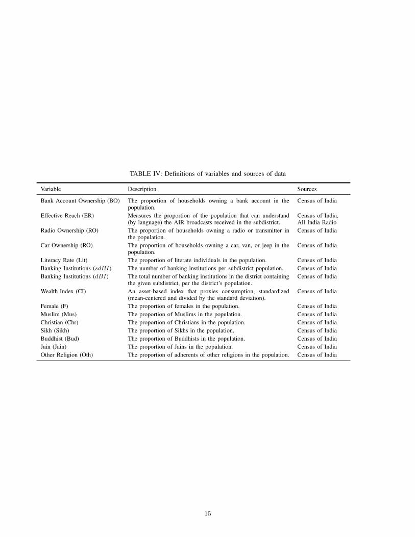
TABLE IV: Definitions of variables and sources of data

Variable Description Sources

Bank Account Ownership (BO) The proportion of households owning a bank account in thepopulation.

Census of India

Effective Reach (ER) Measures the proportion of the population that can understand(by language) the AIR broadcasts received in the subdistrict.

Census of India,All India Radio

Radio Ownership (RO) The proportion of households owning a radio or transmitter inthe population.

Census of India

Car Ownership (RO) The proportion of households owning a car, van, or jeep in thepopulation.

Census of India

Literacy Rate (Lit) The proportion of literate individuals in the population. Census of IndiaBanking Institutions (sdBI) The number of banking institutions per subdistrict population. Census of IndiaBanking Institutions (dBI) The total number of banking institutions in the district containing

the given subdistrict, per the district’s population.Census of India

Wealth Index (CI) An asset-based index that proxies consumption, standardized(mean-centered and divided by the standard deviation).

Census of India

Female (F) The proportion of females in the population. Census of IndiaMuslim (Mus) The proportion of Muslims in the population. Census of IndiaChristian (Chr) The proportion of Christians in the population. Census of IndiaSikh (Sikh) The proportion of Sikhs in the population. Census of IndiaBuddhist (Bud) The proportion of Buddhists in the population. Census of IndiaJain (Jain) The proportion of Jains in the population. Census of IndiaOther Religion (Oth) The proportion of adherents of other religions in the population. Census of India

15

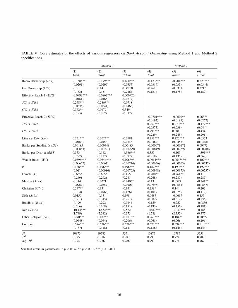
TABLE V: Core estimates of the effects of various regressors on Bank Account Ownership using Method 1 and Method 2specifications.

Method 1 Method 2

(1) (2) (3) (4) (5) (6)Total Rural Urban Total Rural Urban

Radio Ownership (RO) -0.158*** -0.179*** 0.160*** -0.173*** -0.201*** 0.228***(0.0291) (0.0299) (0.0357) (0.0319) (0.033) (0.0344)

Car Ownership (CO) -0.101 0.14 0.00268 -0.261 -0.0331 0.371*(0.133) (0.15) (0.246) (0.157) (0.178) (0.189)

Effective Reach 1 (ER1) -0.0998*** -0.0862*** 0.000923(0.0161) (0.0165) (0.0277)

RO x ER1 0.278*** 0.286*** -0.0718(0.0336) (0.0341) (0.0463)

CO x ER1 0.562** 0.0179 0.349(0.195) (0.207) (0.317)

Effective Reach 2 (ER2) -0.0701*** -0.0600** 0.0637*(0.0192) (0.0189) (0.0257)

RO x ER2 0.257*** 0.270*** -0.177***(0.0375) (0.038) (0.044)

CO x ER2 0.797*** 0.381 -0.434(0.229) (0.245) (0.291)

Literacy Rate (Lit) 0.231*** 0.202*** -0.0581 0.251*** 0.223*** -0.0553(0.0463) (0.0456) (0.0343) (0.0462) (0.0452) (0.0348)

Banks per Subdist. (sdBI) 0.00185 0.000748 0.00483 -0.000071 -0.000172 0.00472(0.00853) (0.00221) (0.00279) (0.00849) (0.00229) (0.00288)

Banks per District (dBI) 0.353 -0.142 -1.386*** 0.335 -0.105 -1.391***(0.797) (0.127) (0.377) (0.818) (0.135) (0.367)

Wealth Index (WI) 0.0896*** 0.0644*** 0.106*** 0.0914*** 0.0647*** 0.107***(0.00657) (0.0061) (0.00744) (0.00656) (0.00605) (0.00737)

θ 0.188*** 0.196*** 0.196*** 0.182*** 0.190*** 0.197***(0.01) (0.00986) (0.00703) (0.00998) (0.00975) (0.00737)

Female (F ) -0.655* -0.685* -0.165 -0.700** -0.761** -0.1(0.269) (0.292) (0.28) (0.268) (0.287) (0.289)

Muslim (Mus) -0.144 0.0271 -0.240** -0.13 0.0329 -0.241**(0.0969) (0.0557) (0.0907) (0.0995) (0.0561) (0.0887)

Christian (Chr) 0.277** 0.131 -0.141 0.258* 0.144 -0.202(0.104) (0.0763) (0.126) (0.101) (0.075) (0.119)

Sikh (Sikh) 0.0156 -0.131 0.198 0.0487 -0.0697 0.157(0.301) (0.315) (0.261) (0.302) (0.317) (0.236)

Buddhist (Bud) -0.199 -0.292 -0.0444 -0.159 -0.252 -0.0856(0.206) (0.168) (0.191) (0.193) (0.156) (0.181)

Jain (Jain) -10.14*** -12.52*** -0.522 -10.87*** -13.33*** -0.488(1.749) (2.312) (0.37) (1.78) (2.352) (0.377)

Other Religion (Oth) 0.270*** 0.182** -0.00137 0.263*** 0.184** 0.00622(0.0648) (0.064) (0.206) (0.061) (0.06) (0.196)

Constant 0.574*** 0.576*** 0.576*** 0.577*** 0.594*** 0.510***(0.137) (0.148) (0.14) (0.138) (0.146) (0.144)

N 10873 10785 5551 10873 10785 5551R2 0.795 0.776 0.787 0.793 0.774 0.788Adj. R2 0.794 0.776 0.786 0.793 0.774 0.787

Standard errors in parentheses: * p < 0.05, ** p < 0.01, *** p < 0.001

16

TABLE VI: Estimates without the Wealth Index (WI)

Method 1 Method 2



Car Ownership (CO) 0.188 0.404** 0.0262 0.155 0.416* 0.358*(0.153) (0.153) (0.227) (0.189) (0.182) (0.151)

Effective Reach 1 (ER1) -0.0881*** -0.0828*** -0.00108(0.0174) (0.0171) (0.0284)

RO x ER1 0.250*** 0.274*** -0.0773(0.035) (0.0352) (0.0457)

CO x ER1 0.287 0.035 0.413(0.221) (0.216) (0.302)

Effective Reach 2 (ER2) -0.0625** -0.0609** 0.0462(0.0204) (0.0196) (0.0257)

RO x ER2 0.209*** 0.242*** -0.168***(0.039) (0.0387) (0.0421)

CO x ER2 0.356 0.0815 -0.327(0.269) (0.252) (0.259)

Literacy Rate (Lit) 0.246*** 0.284*** 0.0963* 0.267*** 0.302*** 0.0957*(0.0473) (0.0446) (0.0488) (0.0473) (0.0444) (0.0478)

Banks per Subdist. (sdBI) -0.0077 -0.000539 0.00758* -0.00939 -0.000759 0.00750*(0.0094) (0.00229) (0.00296) (0.00933) (0.0023) (0.00296)

Banks per District (dBI) 2.129** -0.0797 -1.223** 2.181** -0.0661 -1.238**(0.724) (0.243) (0.421) (0.744) (0.251) (0.415)

θ 0.188*** 0.180*** 0.193*** 0.182*** 0.174*** 0.196***(0.0103) (0.00978) (0.00943) (0.0103) (0.00971) (0.00952)

Female (F ) -0.764** -0.593** -0.0695 -0.801** -0.627** -0.0249(0.293) (0.227) (0.0574) (0.293) (0.229) (0.0616)

Muslim (Mus) -0.244* 0.0382 -0.349*** -0.240* 0.0431 -0.352***(0.1) (0.0669) (0.0737) (0.102) (0.068) (0.0723)

Christian (Chr) 0.112 0.0189 -0.247 0.116 0.0356 -0.307*(0.115) (0.0772) (0.137) (0.112) (0.076) (0.131)

Sikh (Sikh) 0.419 -0.0133 0.233 0.47 0.0211 0.191(0.331) (0.312) (0.344) (0.333) (0.314) (0.317)

Buddhist (Bud) -0.153 -0.274 -0.225 -0.111 -0.231 -0.267(0.192) (0.153) (0.189) (0.18) (0.144) (0.188)

Jain (Jain) -6.707*** -10.09*** 0.283 -7.455*** -10.96*** 0.348(1.661) (2.212) (0.451) (1.681) (2.248) (0.465)

Other Religion (Oth) 0.244*** 0.177* -0.0726 0.242*** 0.178** -0.0636(0.067) (0.0693) (0.176) (0.0651) (0.0662) (0.168)

Constant 0.611*** 0.486*** 0.420*** 0.610*** 0.487*** 0.374***(0.15) (0.115) (0.0446) (0.151) (0.117) (0.0425)

N 10873 10785 5551 10873 10785 5551R2 0.785 0.769 0.754 0.784 0.767 0.754Adj. R2 0.785 0.769 0.753 0.783 0.767 0.753


17

TABLE VII: Estimates without Car Ownership (CO)

Method 1 Method 2



Effective Reach 1 (ER1) -0.0821*** -0.0868*** 0.0255-0.0139 -0.0146 -0.0134

RO x ER1 0.247*** 0.290*** -0.101***-0.0281 -0.0301 -0.0278

Effective Reach 2 (ER2) -0.0442** -0.0493** 0.0306(0.0167) (0.017) (0.016)

RO x ER2 0.213*** 0.256*** -0.129***(0.0316) (0.0344) (0.0304)


Banks per Subdist. (BIsd) 0.00637 0.00088 0.00477 0.00471 0.000693 0.00472(0.00895) (0.00228) (0.00278) (0.00886) (0.00224) (0.00284)

Banks per District (BId) 0.372 -0.143 -1.379*** 0.404 -0.136 -1.366***(0.809) (0.128) (0.378) (0.828) (0.133) (0.374)

Wealth Index (WI) 0.0895*** 0.0660*** 0.107*** 0.0903*** 0.0660*** 0.107***(0.00654) (0.00597) (0.00745) (0.00653) (0.0059) (0.00745)

θ 0.190*** 0.197*** 0.200*** 0.184*** 0.191*** 0.201***(0.01) (0.00984) (0.00719) (0.00996) (0.00974) (0.00716)

Female (F ) -0.589* -0.654* -0.106 -0.629* -0.711* -0.0665(0.264) (0.291) (0.281) (0.263) (0.287) (0.288)

Muslim (Mus) -0.144 0.0283 -0.251** -0.136 0.0355 -0.252**(0.0965) (0.0557) (0.0949) (0.0992) (0.0564) (0.0949)

Christian (Chr) 0.263** 0.141 -0.152 0.284** 0.159* -0.155(0.1) (0.0743) (0.12) (0.0992) (0.0742) (0.121)

Sikh (Sikh) -0.218 -0.193 0.151 -0.191 -0.179 0.149(0.261) (0.311) (0.231) (0.262) (0.31) (0.23)

Buddhist (Bud) -0.198 -0.303 -0.0421 -0.16 -0.259 -0.0367(0.204) (0.166) (0.186) (0.192) (0.155) (0.186)

Jain (Jain) -10.17*** -12.48*** -0.507 -10.99*** -13.38*** -0.469(1.743) (2.314) (0.371) (1.776) (2.354) (0.374)

Other Religion (Oth) 0.266*** 0.181** -0.011 0.266*** 0.182** -0.00358(0.0641) (0.0646) (0.205) (0.0615) (0.0607) (0.202)

Constant 0.543*** 0.564*** 0.550*** 0.539*** 0.569*** 0.525***(0.135) (0.147) (0.141) (0.135) (0.146) (0.144)

N 10873 10785 5551 10873 10785 5551R2 0.794 0.776 0.786 0.792 0.774 0.786Adj. R2 0.794 0.775 0.785 0.792 0.773 0.786


18

TABLE VIII: Estimates without Banking Institution variables (sdBI & dBI)

Method 1 Method 2



Car Ownership (CO) -0.105 0.132 -0.00412 -0.267 -0.0279 0.359(0.133) (0.147) (0.24) (0.157) (0.175) (0.187)


RO x ER1 0.279*** 0.287*** -0.0762(0.0337) (0.0337) (0.0458)

CO x ER1 0.568** 0.0368 0.353(0.195) (0.203) (0.31)

Effective Reach 2 (ER2) -0.0703*** -0.0598** 0.0649*(0.0191) (0.0189) (0.0256)

RO x ER2 0.258*** 0.269*** -0.181***(0.0375) (0.0377) (0.044)

CO x ER2 0.804*** 0.369 -0.419(0.229) (0.239) (0.288)


Wealth Index (WI) 0.0902*** 0.0644*** 0.106*** 0.0920*** 0.0647*** 0.107***(0.00651) (0.00606) (0.00743) (0.00651) (0.00603) (0.00736)

θ 0.189*** 0.196*** 0.194*** 0.183*** 0.190*** 0.196***(0.00993) (0.00979) (0.00709) (0.00988) (0.00968) (0.0074)

Female (F ) -0.657* -0.653* -0.0265 -0.701** -0.728** 0.0396(0.269) (0.284) (0.31) (0.268) (0.279) (0.317)

Muslim (Mus) -0.111 0.0246 -0.238** -0.0985 0.0311 -0.239**(0.106) (0.0548) (0.0905) (0.108) (0.0555) (0.0884)

Christian (Chr) 0.280** 0.13 -0.137 0.261** 0.144 -0.197(0.104) (0.0762) (0.125) (0.1) (0.0749) (0.119)

Sikh (Sikh) 0.0128 -0.134 0.236 0.0457 -0.0647 0.196(0.302) (0.319) (0.273) (0.303) (0.317) (0.248)

Buddhist (Bud) -0.196 -0.296 0.0406 -0.156 -0.255 0.00025(0.205) (0.167) (0.232) (0.192) (0.156) (0.219)

Jain (Jain) -10.17*** -12.51*** -0.513 -10.90*** -13.35*** -0.478(1.745) (2.303) (0.359) (1.777) (2.351) (0.367)

Other Religion (Oth) 0.271*** 0.182** 0.0197 0.264*** 0.183** 0.0282(0.0647) (0.064) (0.204) (0.0609) (0.0601) (0.194)

Constant 0.572*** 0.560*** 0.497** 0.576*** 0.577*** 0.430**(0.137) (0.143) (0.156) (0.138) (0.142) (0.159)

N 10873 10785 5551 10873 10785 5551R2 0.795 0.776 0.785 0.793 0.774 0.785Adj. R2 0.794 0.776 0.784 0.793 0.774 0.785


19

TABLE IX: Estimates without Demographic Variables

Method 1 Method 2



Car Ownership (CO) -0.106 0.119 0.00797 -0.332* -0.0743 0.381*(0.128) (0.15) (0.246) (0.152) (0.185) (0.192)


RO x ER1 0.298*** 0.301*** -0.0742(0.0343) (0.0353) (0.0465)

CO x ER1 0.504** -0.00246 0.357(0.188) (0.209) (0.313)

Effective Reach 2 (ER2) -0.0742*** -0.0662*** 0.0688**(0.0189) (0.0192) (0.026)

RO x ER2 0.275*** 0.280*** -0.182***(0.0382) (0.0398) (0.0437)

CO x ER2 0.860*** 0.403 -0.435(0.225) (0.256) (0.284)


Banks per Subdistrict (sdBI) 0.000898 0.000197 0.00459 -0.0016 -0.000889 0.00462(0.00834) (0.00219) (0.00308) (0.00828) (0.00223) (0.00319)

Banks per District (dBI) -0.0943 -0.0322 -1.273*** -0.0535 0.0238 -1.289***(0.696) (0.129) (0.296) (0.722) (0.139) (0.298)

Wealth Index (WI) 0.0813*** 0.0596*** 0.111*** 0.0833*** 0.0592*** 0.112***(0.00597) (0.00587) (0.00716) (0.006) (0.00585) (0.00709)

θ 0.191*** 0.197*** 0.191*** 0.184*** 0.190*** 0.193***(0.00976) (0.00967) (0.00754) (0.0096) (0.00951) (0.0078)

Constant 0.243*** 0.241*** 0.433*** 0.226*** 0.223*** 0.395***(0.0226) (0.0221) (0.0329) (0.023) (0.0228) (0.0324)

N 10873 10785 5551 10873 10785 5551R2 0.791 0.772 0.783 0.789 0.769 0.784Adj. R2 0.79 0.772 0.782 0.789 0.769 0.783


20

The European Central Bank’s Monetary Policy Announcement Effecton the Exchange Rate in the Effective Lower Bound Era

Raisa Khadija MuhtarAdvisor: Dr. Gosia Mitka

University of St. Andrews

Abstract— Using a high-frequency event study of the Euro-pean Central Bank’s (ECB) monetary policy announcements forboth the “Press Release” event window and “Press Conference”event window, this paper observes an increasing sensitivityof exchange rate response to monetary policy announcementswindows over the period of 2002 to 2019. This supports the viewthat the ECB has growing influence on the exchange rate in theEffective Lower Bound era. The multi-dimensional surprisesidentified in both conventional and unconventional monetarypolicy announcements have all resulted in exchange rate ap-preciations across all currency pairs by successfully increasingthe market’s expectations of future monetary policy via drivingup inflation expectations. Overall, the ECB’s communication ofmonetary policy decisions may be negating the intended effectsof its monetary policy implementation to stimulate inflation,therefore impairing it from achieving its central mandate ofmaintaining price stability.

I. INTRODUCTION

From the viewpoint of monetary policymakers, under-standing the extent to which central banks can influenceexchange rates is important for gauging the effective-ness of monetary policy transmission mechanisms in openeconomies. Adding to that, central banks are changing thefinancial market environment by cutting interest rates to zeroand negative rates and entering the “Effective Lower Bound”(ELB) era. They have also been increasingly utilizing avariety of unconventional monetary policy tools since the2009 financial crisis (Ferrari et al., 2017).

This paper investigates the extent to which the EuropeanCentral Bank (ECB) influences Euro exchange rates in suchan environment. In particular, the paper aims to investigatethe following in the sample period of 2002-2019: (i) thedimension of the ECB monetary policy announcement withthe strongest response on exchange rates, (ii) whether theresponse has changed over time, and (iii) if there is anyheterogeneity of responses across exchange rates. In thispaper, monetary policy is defined as actions of the centralbank that affect the term structure of Euro Overnight IndexSwap (OIS) rates and bond yields. This paper extends andimproves upon the investigation by Altavilla et al. (2019) ofECB monetary policy announcement effects on the nominalspot EUR/USD exchange rate by also including two of thehighest traded Euro cross-currency pairs; that is, EUR/GBPand the EUR/JPY exchange rates (BIS, 2019).

In carrying out this investigation, the paper looks at thenarrow high-frequency response of OIS rates, bond yieldsand nominal exchange rates across two event windows of

ECB monetary policy announcements; the “Press Release”Window and the “Press Conference” Window. Assumingmonetary policy is set endogenously through a Taylor rule,this paper uses a yield factor model regressing on exchangerates to untangle the multidimensional effects of conventionaland unconventional monetary policy announcements chang-ing inflation expectations on the exchange rate.

The different components of the “Press Release” windowand the “Press Conference” window are as identified byAltavilla et al. (2019). Specifically, they have identified 1dimension in the “Press Release” window; that is, the marketreaction to the change or lack of change on the key policyinterest rate named a “Target” surprise. In the “Press Confer-ence” window, they have identified 3 dimensions capturing3 other aspects of ECB monetary policy. One dimension ofthe monetary policy announcement corresponds to the adjust-ment of policy expectations in a way that leaves unchangedlonger-term expectations (the “Timing” surprise), anothercorresponds to changes in the expectations of the mediumrun future short rates (the “Forward Guidance” surprise), andanother corresponding to the changes in long term interestrates (the “Quantitative Easing” or ”QE” surprise).

Following the multi-dimensional monetary policy identi-fication by Altavilla et al. (2019), this paper estimates theexchange rate response to the money market rates using arecursive OLS regression across 3 sub-samples. The sub-samples are the pre-financial crisis period (2002-2007), thefinancial crisis period (2008-2013), and the post-financialcrisis period (2014-2019). Overall, this paper supports thestandard view among financial market participants that theECB has a growing influence on the exchange rate throughits monetary policy communication. In support of the conclu-sion by Altavilla et al. (2019), the paper observes growingsensitivity of the exchange rate response to monetary pol-icy announcements in the post ELB era. The conventionalsurprise in the form of the “Target” factor as well as theunconventional surprises captured in the “Timing”, “ForwardGuidance” and “QE” factors have all resulted in exchangerate appreciations across all currency pairs. Importantly, thispaper also quantifies the effect of each surprise on theexchange rate within its corresponding period. This is doneby each surprise increasing the market’s expectations offuture monetary policy via driving up inflation expectations.This paper also shows that “Forward Guidance” has had thelargest appreciation effects on the exchange rate.

21

While most of the literature has focused on analyzing theinfluence of central bank actions on the exchange rate, thispaper’s analysis of the announcement effect of ECB mone-tary policy communication extends the literature by showingthat the ECB is increasingly influencing the exchange ratethrough monetary policy announcements themselves. Thispaper finds that the ECB’s communication of monetarypolicy decisions may be negating the intended effects of itsmonetary policy action implementation to stimulate inflationand therefore impairing it from achieving its central mandateof maintaining price stability. It presents an interesting trade-off with the preceding announcement effect of monetary pol-icy decisions depressing current inflation levels, contrastingthe monetary policy implementation effects of stimulatinginflation.

II. LITERATURE REVIEW & JUSTIFICATION

A. Methods of measuring monetary surprises.

In analyzing monetary policy surprises, the main empiricalchallenge is an endogeneity problem; that is, the problemthat the analysis may not isolate the effect of the monetarypolicy surprise itself and instead include effects caused byother surprises. In what follows, I will explain the two mainapproaches in the literature that try to measure the monetarypolicy surprise whilst countering this endogeneity effect. Thefirst is a vector autoregression (VAR). The second methodand the applied method of this paper is a high-frequencyidentification event study (henceforth, H-F approach).

A VAR attempts to overcome the endogeneity problemby placing timing and impact restrictions on the interactionbetween the policy rate and other financial market or realeconomy variables (Jardet and Monks, 2014). This approachhas been used in studies such as Cardona (2014) and Strakevaand Tang (2015). However, the concern with this approachis the persistence of endogeneity despite attempts to controlfor it (Nakamura and Steinsson, 2018). Another concern isVAR overidentification, and the literature endorses imposingtheory-relevant restrictions in VAR estimation (Strakeva andTang, 2015).

An H-F approach is a market-based approach focusingon movements in asset prices in a narrow window aroundscheduled central bank announcements. First established byCook and Hahn (1989), it has since been widely used toinvestigate the effect of monetary policy on exchange rates. Itinvolves running an OLS regression, regressing movementson asset prices on key surprise-identifying instruments asvariables. The regressions are of the form:

∆st = α+ βsurprise + εt (1)

where ∆st is the (log) change in the nominal exchange ratearound the policy announcement and εt captures the changesin st not due to monetary policy. The estimated coefficientscan be interpreted as follows: a one-percentage-point factorsurprise is associated with a 100 ∗ β percent change in theexchange rate (Ellen et al., 2017).

A focus on changes in exchange rates in a narrow windowaround scheduled central bank meetings is important becauseit allows βsurprise to only respond to surprises relating tomonetary policy announcement decisions without reacting toother economic news during that period. Specifically, sincethis paper considers only a specific subset of all observations(in this case, only days of central bank monetary policyannouncements), it will yield an unbiased estimate as thevariance of the monetary policy surprise is infinitely large inthe limit relative to the variance of other surprises on centralbank monetary policy announcement dates. This permitsa discontinuity-based identification scheme (Nakamura andSteinsson, 2018). Hence, the narrow window delivers anapproximate natural experiment and allow better mapping ofthe exchange rate response by better controlling for reversecausality and omitted variables (Faust et al., 2007). Otherassumptions implicit with the adoption of a narrow windoware that financial markets integrate all the information re-leased by the central bank immediately and that risk premiaentrenched in asset prices do not change (Cecioni, Martina2018).

B. Theoretical literature review.

This paper will consider a suitable monetary model ofexchange rate determination as a framework for understand-ing the effect of inflation expectations on nominal exchangerates. This paper will first present the Frankel (1983) Mon-etary Model of Exchange Rate Determination, and thencontrast it to the New Keynesian Engel and West (2006)model used in this paper. While both approaches similarlyinclude home and foreign interest rate differentials, inflationand output gaps in the exchange rate determination, bothhave different conclusions about the direction of inflationexpectations’ influence on the exchange rate.

The Frankel (1983) model is derived under perfect in-formation, with the only shock originating from an initialmonetary policy surprise. The instrument of monetary policyis money supply, exogenous to the model. The moneydemand functions are as follows:

m = p+ γyy − γiE(i) (2)m∗ = p∗ + γyy

∗ − γiE(i∗) (3)

where m and m∗ are the logarithms of the home and foreignmoney supply, y and y∗ are the logarithms of home andforeign real output, i and i∗ are the home and foreign interestrates, and E denotes the expectation of a random variable.γy is the elasticity of income and γi is the elasticity of theinterest rate. Assuming prices are flexible in the long run,this means that Purchasing Power Parity (PPP) holds:

s = p− p∗ (4)

where s is the (log) of the nominal spot exchange rate usingthe price quotation system with units of home currency perunit of foreign currency and p and p∗ are (logs) of the homeand foreign price levels all at time t. Assuming UncoveredInterest Parity (UIP) holds:

22

∆E(s) = i− i∗ (5)

Here, an expected depreciation of the home currency is equalto the nominal interest rate differential between home andforeign. Since PPP holds:

∆E(s) = E(π − π∗) (6)

Here, the expected depreciation of the home currency isequal to the expected difference between home and foreigninflation rates at time t. Thus, the representation of theflexible price monetary equation is as follows:

s = (m−m∗) − γy(y − y∗) + γπE(π − π∗) (7)

Now, γπ replaces γi as the elasticity of expected inflation.Hence, the exchange rate is a function of money supplyand demand. Increases in the domestic money supply causeexchange rate depreciation and increases in money demandresulting from either an increase in domestic output or adecrease in the expected inflation rate cause an appreciationof the home currency.

Since this paper is investigating the central bank announce-ment effect on the exchange rate around a narrow window,the paper will thus follow the sticky price assumption in theshort run. Frankel presents an exchange rate determinationmodel that incorporates Dornbush’s (1976) “overshooting”model where in the short run, the nominal spot exchangerate deviates from its long run equilibrium value. Here, theexchange rate in the short run adjusting toward equilibriumat a rate proportional to the inflation expectation gap:

∆E(s) = −θ(s− s) + π − π∗ (8)

Here, θ is the speed of adjustment, and a bar over variablesshow a relationship that holds in the long run. Combine thiswith the UIP assumption in (5), we have an expression forthe gap between the current spot rate and its equilibriumlevel:

s− s = −1

θ[(i− π) − (i∗ − π∗)] (9)

Following (9), a contractionary monetary policy shouldraise the real interest differential, attracting a capital inflowand subsequently appreciating the currency above its equi-librium value. Frankel 1983 thus combines equations (8) and(9) to obtain the sticky-price monetary equation of exchangerate determination:

s =(m− m∗) − γy(y − y∗)

+ (γπ +1

θ)(π − π∗) − 1

θ(i− i∗) (10)

The interpretation of the equation remains the same, withthe factors affecting the money supply and demand affectingthe exchange rate in the same way and direction. Assuming

that in a narrow window around central bank announcements,m and m∗, y and y∗, i∗ and π∗ would remain fixed. Thus, theonly change would result from a long-run change in the homeexpected inflation and the home interest rate. In particular:

δs > 0 (i.e., a home currency depreciation occurs) if

(γπ +1

θ)δπ >

1

θδi (11)

δs < 0, (i.e., a home currency appreciation occurs) if

(γπ +1

θ)δπ <

1

θδi (12)

However, this paper finds that in the ELB era, this resultdoes not hold empirically. Cesa-Bianchi et al. (2019) arguethat this is due to the assumption that interest rate policyis exogenous rather than being determined by a policy rulethat responds systematically to economic conditions. Thus,we will require a New Keynesian model with the interestrate as the instrument of monetary policy to aid explanationof exchange rate movements in the ELB era.

The model used in this paper is by Engel and West (2006)who specify a New Keynesian model. Here, the interest rateis endogenously set according to a policy rule, where ittypically reacts to a change in the inflation and the outputgap. Assuming monetary policy is set using a Taylor rule forboth Home and Foreign:

it = rt + γππt + α(it−1 − rt−1) (13)i∗t = rt

∗ + γππ∗t + α(i∗t−1 − r∗t−1) (14)

The time subscript t is added to denote variables correspond-ing to a specific period. We also specify πt and π∗t as thehome and foreign inflation, rt and rt

∗ as the home andforeign real interest rate if prices adjusted instantaneouslyand 0 ≤ α < 1 as the coefficient of interest rate differentials(Engel, 2014). For both home and foreign, an increase ininflation or the output gap would lead to an increase in thepolicy interest rate. Following that, the new modified Taylorrule with domestic relative to foreign as according to Engeland West (2006) is:

it − i∗t = γqqt + γπEt(πt+1 − π∗t+1) + γy(yt − y∗t ) (15)

Here, qt is the real exchange rate at time t, γq is the elasticityof the real exchange rate and yt and y∗t denote the homeand foreign output gap. Also, the UIP condition showing theindifference of an investor between deposits in two countriesis:

it − i∗t = Etqt+1 − qt + Et(πt+1 − π∗t+1) (16)

Combining (15) and (16) to solve for the real exchangerate in terms of the present values of current and expected

23

future inflation and output gaps, we arrive at:

qt = −∞∑

j=1

(1

1 + γq)jEt[

(γπ − 1)

1 + γq(πt+j+1 − π∗t+j+1)

+γy

(1 + γq)(yt+j − y∗t+j)] −

1

1 + γqεt (17)

Based on the Taylor rule and UIP condition, Engel andWest (2004) present forward-looking determinants of ex-change rates. The assumptions made are that at least one ofthe countries responds to the exchange rate misalignment andPPP holds in the long-run. Thus, the interest rate responds tochanges in the real exchange rate and raises the interest ratewhen expected inflation or the expected output gap is higher.When the stability condition γπ > 1 holds, the interestrate rises enough to result in an increase real interest rates,causing a real appreciation.

As prices do not adjust over the short term, the changein qt originates exclusively from changes in the nominalexchange rate, represented by st+∆ − st−∆. Thus, (17)becomes:

st+∆ − st−∆ ≈−∞∑

j=1

(1

1 + γq)j(Et+∆ − Et−∆)

[((γπ − 1)

1 + γqπt+j+1 − π∗t+j+1)

+γy

1 + γq( ˜yt+j − ˜y∗t+j)] (18)

The model assumes that the actual inflation and outputgap, πt−π∗t and yt−yt∗,do not change between t−∆ and t+∆. Thus, changes in exchange rate over the narrow windoware driven only by expectations of future relative inflationrates and output gaps. Given that γq > 0, γπ > 1 and γγ >0, then the Taylor rule model infers that a higher expectedinflation or a higher output gap in the home country will leadto a home real appreciation (Engel, 2014). Given this result,this paper can investigate the extent to which ECB monetarypolicy announcements are influencing the Euro exchange rateby adjusting market inflation expectations.

C. Empirical literature review.

This paper relates to various strands of literature analyzingthe market reaction to the announcement of policy decisions.Most of the work has focused on the effect of FederalReserve Open Market Committee (FOMC) announcementsurprises and has only recently expanded to the announce-ment effects of other central banks. The literature mostlyagrees that financial-market reactions to monetary policyannouncements are significant (Ehrmann and Fratzscher,2007).

This paper primarily follows Cook and Hahn (1989), whostudied the day change of the Federal Funds key policyrate on bond yields in the 1970s. They concluded that theFOMC has strong influence on market interest rates throughits control of the funds rate and that the expectations ofthe future level of the funds rate strongly influence othermoney market rates. Kuttner (2001) built upon Cook and

Hahn (1989) by instead isolating the surprise component ofthe change in monetary policy by using the intraday FedFunds futures rate as a measure of the expected interest raterather than the intraday change in the key policy interest rateto identify the impact of a monetary policy decision.

Following Kuttner (2001), this paper investigates howexchange rate changes are affected by adjustments of futuremonetary policy expectations as proxied by market interestrates. One such study is conducted by Zettlemeyer (2004),who applies the event study methods from Cook and Hahn(1989) to study the effect of central bank monetary pol-icy announcement effects in Australia, New Zealand andCanada on USD/AUD, USD/CAD and USD/NZD usingdaily data from 1990-2000. He finds evidence to supportthe conventional relationship between exchange rates andmonetary policy surprises; that monetary contractions lead toexchange rate appreciations and monetary expansions lead todepreciations. By contrast, Fatum and Scholnick (2006) usea generalized autoregressive conditional heteroskedasticity(GARCH) time-series approach to study the effects of FOMCannouncement days and non-FOMC announcement dayson the USD/JPY, USD/GBP and USD/Deustchemark from1989 to 2001 via the change in the Fed Funds rate. Theyalso control for 6 US macroeconomic news announcements,interest rate changes and foreign exchange interventions fromother central banks. They find that changes in expectationsof future monetary policy affect exchange rates and thatan increase in the expectation of the future Fed Funds rateresults in a dollar appreciation.

This paper contrasts itself to Zettlemeyer (2004) in 2 ways.Although this paper also uses an event study and defines“surprises” as changes in the market interest rate associatedwith a given policy announcement, this paper extends anal-ysis of exchange rate responses to ECB monetary policy.This paper will use a narrower window of intraday data asopposed to daily data, improving control for endogeneityand omitted variable bias. Also, in contrast to Zettlemeyer(2004) and in line with Fatum and Scholnick (2006), thispaper will examine the effect of how changes in expectationsof future monetary policy affect exchange rates. Contrastingboth Zettlemeyer (2004) and Fatum and Scholnick (2006),the paper will also examine the exchange rate responses post-2008.

This paper also follows Gurkayanak et al. (2005), whostudy the effects of monetary policy announcements on bondyields and equities using an intraday sample of announce-ments from 1990-2004 and use factor identification to extendthe single factor of monetary policy to two factors. One factorrelates to policy surprises called the “Target” factor, andthe other component relates to expected future policy ratesorthogonal to the “Target” surprise called the “Path” factor.They confirm that surprises related to the future path of mon-etary policy are an important driver, particularly for longer-term bond yields. Swanson (2017) extends Gurkayanak etal. (2005) by separately identifying a “target” surprise cor-responding to surprise from the change in the fed fundsrate, “forward guidance” as a factor affecting medium-term

24

maturities and “large-scale asset purchases” factor affectinglong-term maturities for all FOMC announcements to capturethe effects of the new unconventional monetary policy toolemployed in new ELB period during 2009-2014.

With the identification of new monetary policy announce-ment dimensions associated with the new ELB era, Ferrari etal. (2017) conduct a high-frequency event study of monetarypolicy on the exchange rate for 7 advanced economiesusing factors identified as in Gurkayanak et al. (2005)and Swanson (2017). They analyze USD/EUR, USD/JPY,USD/GBP, USD/CHF, USD/AUD and USD/CAD responsescorresponding to tight windows of various announcements ofthe respective 7 central banks in a sample period of 2004-2015. They find that exchange rate sensitivity in respondingto monetary policy has increased over time and that the dropin interest rates signifying the ELB period contributes to theincrease in sensitivity. However, Ferrari et al. (2017) do notinclude an analysis of market reactions to the ECB pressconference and simply considers the press release marketreaction. Using the identification pioneered and extended byGurkayanak et al. (2005) and Swanson (2017), this paperdistinguishes itself from Ferrari et al. (2017) by insteadfocusing on a specific ECB analysis of the market reactionfor both the ECB “Press Release” event with the ECB“Press Conference” window, observing the Euro exchangerate response for both.

Distinguishing asset price and money market interest ratemovements specific to ECB “Press Release” with the ECB“Press Conference” is made possible with Altavilla et al.(2019)’s paper on ECB monetary policy announcement ef-fects featuring the construction of an event-study datasetof the ECB monetary policy announcements from 2002-2018. Analyzing a sample from 2002-2018, they extend theliterature analyzing multi-dimensional central bank monetarypolicy communication specific to the ECB. They show thatone factor, the “Target” surprise with a unit effect on the one-month OIS captures all the variation in the money marketrates the “Press Release” window. By contrast, three factorscapture nearly all the discrepancy in the market rates forthe press conference, with the “Timing” effect on six-monthOIS, “Forward Guidance” (“FG”) having unit effect on thetwo-year OIS and “QE” having a unit effect on the ten-yearOIS.

Given these results, this paper follows Altavilla et al.(2019) by employing their dataset and identified factors forthe “Press Release” window and the “Press Conference”window to analyze exchange rate responses to ECB monetarypolicy announcements. However, this paper distinguishesitself from Altavilla et al. (2019) in 3 ways. First, thepaper extends the baseline EUR/USD response analysisprovided in Altavilla et al. (2019) by including an analysisof the monetary policy announcement response of EUR/GBPand EUR/JPY for the pre-crisis, financial crisis, and post-financial crisis periods to determine if there is a heterogeneityof responses across cross-currency pairs. Second, this paper’sanalysis includes the 2019 period. Finally, this paper replacesthe 10-year OIS as the identifying “QE” surprise with the

10-year German bond yield as a more accurate moneymarket instrument to measure the changes in monetarypolicy expectations. This paper’s analysis of the exchangerate responses to ECB monetary policy announcements willbe supplemented with the Engel and West (2006) modelpresented in Section 2.2, concluding as Fatum and Scholnick(2006) do that the announcement of monetary policy actionsthat alter expectations of future monetary policy influenceexchange rates.

III. ECB MONETARY POLICY

A. The ECB’s conventional monetary policy.

Since the ECB’s founding in 1999, its main mandate hasbeen to maintain price stability in the Eurozone, defined asinflation close to, but below 2% (ECB, 2011). As the prin-cipal issuer of the Euro, it ultimately controls the monetarybase and manages liquidity in the money market.

The ECB has three key interest rates; the marginal lendingrate, the short-term repo rate, and the overnight deposit rate(ECB, 2011). Key interest rate changes, which comprise theECB conventional monetary policy toolkit affect the shortestmaturities and peak around the one-month maturity of theyield curve . Their evolution over time can be seen in Figure1 in Appendix A. Beginning March 2009 with the onsetof the global financial crisis, key interest rates substantiallydropped to 0.5% and even reached negative territory, sig-nifying the ELB era. Ever since, monetary policy has beenunsuccessful in its attempts to stimulate inflation and aggre-gate demand exclusively via conventional monetary policy.As a result, the ECB has since increasingly supplementedits expansionary conventional measures with unconventionalmeasures in order to stimulate inflation (ECB, 2011).

B. The ECB’s unconventional monetary policy.

To date, the ECB has introduced a few unconventionalmonetary policy measures, and this paper will focus ontwo of these measures. In hopes of encouraging more openand transparent communication of future policy to affectmedium-term market rates in the deflationary Euro-areaeconomies, the ECB began to implement forward guidancein July 2013 to clarify the ECB’s intentions not only aboutthe expected future path of the ECB’s key interest rates, butalso the horizon of its asset purchase program (ECB, 2017).

The ECB’s asset purchase program was introduced inJanuary 2015, a liquidity improving action affecting longer-term rates known as QE (ECB, 2011). It is executed throughthe purchase of long-term government bonds and financedby an increase in the reserve accounts held by commercialbanks within the central bank. The hope is for the measureto aid in providing a monetary stimulus by increasing long-term bond prices and therefore lowering long-term yields inthe ELB era.

Swanson (2017) found that both forward guidance and QEhave a hump-shaped effect on the yield curve. Specifically, hefound that forward guidance manifests this hump-shape withits largest effect on shaping market expectations at two to fiveyears maturity, whilst leaving both current short and expected

25

short rates far into the future unaffected. In contrast, QEannouncements have their largest effect on shaping marketexpectations further into the future, peaking at around theten-year maturity.

C. The institutional characteristics of ECB monetary policyannouncements.

ECB monetary policy announcements have a clear segre-gation of news regarding the key policy rates and the com-munication of details regarding their decision. This enablesclear analysis by specifically identifying different types ofmonetary policy news and their respective impacts on theexchange rates, making it ideal for an H-F approach (Brandet al., 2010).

During the ECB’s inception in 1999, the ECB GoverningCouncil announced policy decisions twice a month, whilea press conference took place only once a month at thefirst meeting of the month (Altavilla et al., 2011). AfterNovember 2001, policy meetings were rescheduled to once amonth, specifically, the first Thursday of every month. Thesemonthly meetings were accompanied by press conferences,with minimal exceptions (Ehrmann and Fratzscher, 2009).Since January 2015, monetary policy announcements haveevolved to a six-week cycle.

Monetary policy is communicated in two separate eventson Governing Council announcement days. The first eventis a brief online press release describing what action wastaken (or not taken) on the key policy interest rate at 13:45,Central European Time. Since the decision contains nothingabout the ECB’s future policy or outlook, it is reasonableto assume that market movements are reacting instantlyafter the press release, with the reaction relating only toimmediate policy changes. However, the ELB period afterMarch 2009 may alter the market movement responses tothis event window since the interest rate remains effectivelyunchanged. On top of that, March 2016 marked a change inthe communication of the Press Release with the introductionof description of changes in both the target rate as wellas a description of unconventional measures the ECB ismaking. Thus, the decision after this period should reflectboth immediate policy changes and the future path of policy,which is not accounted for in this paper in the analysis ofthe “Press Release” event.

The second event, a “Press Conference” is held at 14:30and lasts 15 minutes. Here, the ECB President explains themonetary policy decision in detail. It begins with a statementsummarizes and explains both monetary policy developmentsand the monetary policy decision of the Governing Coun-cil (Ehrmann and Fratzscher, 2009). Then, at 14:45, thePresident answers journalists’ questions relating mainly toconsiderations contributing to the policy decision (Brandet al., 2010). Similar to Altavilla et al. (2019), this paperwill assume that market reactions to the “Press Conference”event are reactions that relate to the future path of policy,since investors have already accounted for target rate changesfollowing the press release.

IV. DATA

A. Euro Overnight Index Swaps (OIS) as a measure ofmonetary policy expectation.

Given this paper’s definition of monetary policy, it isimportant to explain OIS, the primary interest rate usedin this paper and associated benefits of using this marketinterest rate as a measure of a market participant’s interestrate expectations.

OIS is the average Euro Overnight Index Average (EO-NIA) expected at a given maturity. These instruments area combination of expectations of future short-term interestrates and a term premium. While expectations of monetarypolicy actions are not directly observable, OIS rates are agood market-based proxy for those expectations.

The exchange of an OIS involves one institution swappinga floating interest rate and the other swapping a fixed short-term interest rate at a given maturity. In the absence ofarbitrage opportunities, OIS should reflect the minimal risk-adjusted market participants’ expectation of the average pol-icy rate over the swap maturity, since the principal remainsunexchanged between the parties (Hubert and Labondance,2018). Additionally, despite market-based interest rates in-corporating a risk premium, the change in the market interestrate remains a good proxy for the policy surprise since therisk premium is unlikely to move in the narrow window ofthe event study specified in this paper. Thus, a measure of thechange in the OIS rate as used in this paper would excludethis risk premium.

Notably, Lloyd (2018) shows that OIS Euro Area-wideinterest rates at 1- to 2-year maturities provide accuratemeasures of investors’ interest rate expectations. Comparedto fixed-rate bonds, OIS rates are less volatile. However,Lloyd (2018) also warns that OIS rates beyond 2 years showpositive and statistically significant ex-post excess returns,indicating the presence of term premia characteristic oflonger-maturity contracts. This marginally diminishes theirusefulness as a market-based measure of monetary policyexpectations and may make them a biased proxy of theQE effect. Thus, contrary to Altavilla et al. (2019) andin line with Ferrari et al. (2017), I will be replacing theOIS-10 year with the German 10-year Bund as a factorrepresenting the 10-year maturity instrument. As the largesteconomy in the Eurozone, the German 10-Year Bund quotesshould be representative of Euro-area bond yields. Whilst theOIS ceases to be traded beyond 2-year maturities, the highmarket liquidity of German 10-year Bund will decrease theterm premia and volatility stemming from reduced liquidityrisk, making them a better proxy for the QE surprise incomparison to the 10-year OIS (Bundesbank, 2018).

B. Euro Area Monetary Policy Event-Study Database (EA-MPD).

The underlying data for this paper originates from theEA-MPD database compiled by Altavilla et al. (2019). Thedatabase features policy news reaching the financial marketscorresponding to the institutional features of ECB monetary

26

policy communication via the “Press Release” and “PressConference” windows as specified in Section 3.3. This paperwill specifically make use of their OIS 1-month, 6-month and2-year quotes, their German 10-year bund quotes, replacing10-year OIS as better market interest rate instrument than inAltavilla et al. (2019), as well as their EUR/USD, EUR/GBPand EUR/JPY exchange rate crosses. All data is quoted inbasis points. As an example, the OIS quotes in the EA-MPDare calculated as follows:

∆MPSurpriset =OISmedian[t+20min; t+10min]

– OISmedian[t–10min; t–20min] (19)

The equation shows a change in the median OIS interestrate in 20 minutes to 10 minutes pre-press-release, to thechange in the median OIS interest rate 10 minutes to 20minutes post-press-release quote. In other words, the ratesetting surprise can be expressed as the change in two OISobservations defined as above, denoted as MPSurpriset.Similarly, the EA-MPD takes the change in the median OISinterest rate in 20 minutes to 10 minutes pre-press conferencequote, to the change in the median OIS interest rate 10minutes to 20 minutes as the post-press-conference quote.Other bond yields and currency cross quotes used in thispaper are calculated in corresponding fashion.

V. METHOD

A. Decomposing policy surprises.

Following the identified factors as in Altavilla et al. (2019),the regressions can be formed specific to the “Press Release”and “Press Conference” event windows using the generalOLS regression form specified in Section 2, equation (1).The regressions that follow will be implemented for saidevent windows across 3 sub-samples. These sub-samples arethe pre-financial crisis period (January 2002 until December2007), the financial crisis period (January 2008 until Decem-ber 2013), and the post-financial crisis period (January 2014until June 2019) to observe if there is a difference in theresponse before and after the ELB.

For the “Press Release” event window, the paper regressesthe (log) exchange rate changes on the “Target” surprise:

∆st = α+ βtarget · (MPSurpriseOIS1Mt )︸︷︷︸

Target Surprise

+ εt (20)

where, for event t, MPSurpriseOIS1Mt is the change in

the 1-month OIS interest rate. Here, ∆St is the change inthe (log) exchange rate defined as units of foreign currencyper unit of home currency, following the volume quotationsystem. Therefore, a positive value of the (log) exchange ratechange shows an appreciation of the home currency.

The “Press Conference” event window regression is as

follows:

∆st = α+ βTiming · (MPSurpriseOIS6Mt )︸︷︷︸

Timing Surprise

+ βFG · (MPSurpriseOIS2Y⊥t )︸︷︷︸

Forward Guidance Surprise

+ βQE · (MPSurpriseDE10Y⊥t )︸︷︷︸

QE Surprise

+ εt (21)

The specification here is that MPSurpriseOIS6Mt is the

change in the 6-month OIS interest rate, identifying it asthe “Timing” surprise. The interpretation of the “Timing”surprise, peaking at about six months maturity, is a marketrevision of policy expectations that shifts the expectation ofthe policy action from something that was highly expected tohappen on the day to now more likely to happen during thenext upcoming announcements. Importantly, it leaves longer-term policy expectations unaffected.MPSurpriseOIS2Y⊥

t is the orthogonal change in the 2-year OIS. The change should be driven by expectationsof the medium run future short rates, peaking at about 2-year maturity. The MPSurpriseDE10Y⊥

t is the orthogonalchange in the 10-year German Bund (identifying the “QE”surprise). The “QE” surprise will be largely traced to changesin long-term interest rate, peaking at about 10-year maturity.The “Forward Guidance” surprise is omitted for the pre-financial crisis sample, and the “QE” surprise is omitted inthe pre-financial crisis and the financial crisis samples.

VI. RESULTS AND DISCUSSION

While running both regressions, this paper observes thatmovement in market rates takes place instantly after newson monetary policy decisions becomes available. This isconsistent with literature that finds that the Euro area moneymarket is efficient in incorporating new information rapidly(Brand et al., 2010). All figures and tables referenced in thissection can be found in Appendix A.

A. Results of “Press Release” regression.

Referring to Table 1, Panel (A) and Figure 2, there is aclear heterogeneity of responses for the pre-financial crisisand financial crisis responses for the cross-currency pairs,with more statistically significant homogeneous responsespost-financial crisis. The effect of a 1-unit increase in βtargetduring the pre-financial crisis period of interest rate hikesdid not have a statistically significant effect on EUR/USDbut caused a statistically significant 0.01% appreciation inEUR/GBP and a 0.01% depreciation in EUR/JPY. Prior tothe ELB, increasing interest rate hikes has resulted in lowerfuture inflation expectations resulting in a lower expectedlong run value of euro returns stemming from the Taylor rule,with lower inflation expectations resulting in lower interestrates. This causes the Euro to depreciate against foreigncurrencies, leading to a small and economically insignificant

27

coefficient prior to the ECB beginning their ELB policy asexemplified in the depreciation of EUR/JPY.

By contrast, the financial crisis period showed a sta-tistically insignificant effect for both EUR/USD andEUR/GBP, with a statistically significant 0.02% depreciationin EUR/JPY. While this era was marked by drastic interestrate cuts to stimulate the economy during the crisis, theEUR/JPY depreciation is probably more reflective of marketparticipants moving towards purchasing more Yen currencyto diversify their assets from the impact of the US-bornfinancial crisis, with the Yen currency having the mostnegative correlation to 10-year U.S. Treasury yields.

Post-financial crisis, the effect of a 1 unit increase inβtarget is a statistically significant 0.14% appreciation onaverage across all currency pairs. Post ELB, higher inflation-ary expectations in the future also increases the expectationsof an interest rate hike in the future. Therefore, monetarysurprises originating from the ECB announcements are nowassociated with a statistically significant appreciation of theEuro. It is also worth noting the increased sensitivity of theexchange rate to a “Target” surprise in the post-crisis period,also observed in Figure 2. This may be due to the strengthof the Forward Guidance and QE effects in shaping marketexpectations, particularly in influencing longer term inflationexpectations.

B. Results of “Press Conference” regression.

Referring to Table 1, Panel (B) and Figure 3, the re-gressions show that the “Timing” surprise is only relevantin the pre-financial crisis period, with a 1-unit increase inthe coefficient of the “Timing” surprise (βtiming) having anaverage 0.05% appreciation for all currency pairs. However,during and after the financial crisis, βtiming has lost its placeas a key driver of the exchange rate response, contrary tothe results in Altavilla et al. (2019), that show βtiming assignificant across all three subsamples. This suggests thatmonetary policy announcements no longer leave longer-termpolicy expectations unchanged.

Instead, in the financial crisis and post-financial crisisperiods, the coefficients on the “Forward Guidance” surprise(βFG) and the “QE” surprise (βQE) indicate that these haveemerged as key drivers. The effect of a 1 unit increase in βFGis a 0.04% increase in the exchange rate across all currencypairs, and the effect has strengthened to 0.16% post-crisis.This suggests that expectations of future short-term ratesrelated to monetary policy are a key driver of the exchangerate response, and the significance of central bank forwardguidance affecting the shorter-end of the yield curve (Swan-son, 2014). The strengthened response to forward guidancesurprises post-financial crisis may reflect the effectiveness ofthe enhanced forward guidance adopted by the ECB in June2018 for reducing uncertainty regarding the expected futurepath of short-term interest rates (Cœure, 2018).

The QE effect in the post financial crisis period is signif-icant for EUR/USD and EUR/JPY, with a unit increase inβQE having a 0.04% increase for EUR/USD and a 0.057%increase for EUR/JPY. However, the effect is not significant

for EUR/GBP, suggesting that βQE surprises only transmit tothe EUR/USD and EUR/JPY exchange rates. “QE” surprisesare effectively reducing uncertainty around the expectedfuture path of long-term interest rates for EUR/USD andEUR/JPY, with a smaller magnitude of effect compared toforward guidance.

C. Further discussion.

Overall, the results confirm the prediction in the Engel andWest (2006) model that a currency tends to appreciate whenthere are higher inflation expectations affecting expectedfuture policy rates via the Taylor rule. Specifically, the con-ventional monetary policy announcement surprise captured inthe “Target” factor, coupled with the unconventional mone-tary policy announcement surprises captured in the “ForwardGuidance” and “QE” factors have resulted in a measuredquantifiable appreciation in all the exchange rate pairs. Thisis achieved through their successful transmission of theirmonetary policy tools in increasing inflation expectations inshort, medium and long-term rates.

Contrasting Strakeva and Tang (2015), who, upon ana-lyzing FOMC announcement effects on the exchange rate,concluded that the importance of conventional monetarypolicy in impacting the exchange rate is decreasing relative tounconventional monetary policy during the ELB, this paperfinds the both the ECB conventional and unconventionalmonetary policy surprises have an increased role in explain-ing exchange rate changes since the ELB. The strongestappreciation effects stem from the “Forward Guidance” sur-prise, followed by the “Target” surprise. The “QE” surprisehas the lowest magnitude effect on currency appreciationacross all currency pairs.

Some reasons for the increasing exchange rate sensitiv-ity may also be the reduced liquidity and intermediationability of brokers resulting from changes in regulation post-financial crisis. This in turn leads to the declining willing-ness of market actors to bear inventory risk during high-risk periods of the financial crisis and post-financial crisisyears during central bank announcement days (Ferrari et al.,2017). Another possible driver could be recent technologicalinnovations, such as algorithmic trading tools and faster newstransmission through fibre-optic cables, resulting in fasterprocessing of monetary policy announcement information.

Other observations include the EUR/GBP exchange ratehaving the lowest magnitude of monetary policy announce-ment surprise effect of all the currency pairs. This is observedin the reduced magnitude of the coefficient in the followingsurprises across Panel (A) and Panel (B). Specifically, thetransmission of monetary policy announcement surprises toEUR/GBP is the weakest in the “Target” surprise in thepost financial crisis period, the “Timing” surprise in the pre-financial crisis period, the “Forward Guidance” surprise inthe financial crisis period and the “QE” surprise in the postfinancial crisis period. Future work could explore the reasonsbehind this difference in the response for EUR/GBP andanalyze if the effects are similar for other widely traded Eurocross currency pairs.

28

VII. ROBUSTNESS CHECKS

All regressions have been checked and cleared of multi-collinearity and heteroskedasticity. A robustness check re-placing OIS rates with German bunds is included in Ap-pendix B for “Press Release” and “Press Conference” andshows that the same observations hold.

VIII. POTENTIAL SHORTFALLS OF RESEARCH

A. US initial jobless claims report.

The US weekly Initial Jobless Claims (IJC) is the onlyrepeatedly occurring economic release that coincides withthe ECB monetary policy announcements. Specifically, itis released during the beginning of the “Press Conference”window. As explained in Section 2, other news releasesthat occur during the same period may result in omittedvariable bias in the regression despite the narrow windows.However, both Brand et al. (2010) and Altavilla et al. (2019)evaluated the impact of the US report on the identified factorsof monetary policy announcements and found very small,statistically insignificant coefficients and made no differenceto the coefficients of interest with its inclusion or omissionin the regressions. As such, excluding a control for the IJC inthe “Press Conference” regression should not bias the resultsof this paper.

B. Drawbacks of the H-F approach.

The H-F approach used in this paper is useful to estimateimmediate effects of monetary policy on financial variables.However, estimating longer term persistence of monetarypolicy announcement effects on the exchange rate becomesmuch more difficult with this approach and is beyond thescope of this paper. Future research on analyzing the persis-tence of the monetary policy announcement effects on thesecurrency pairs will require the VAR approach.

C. Possible broader definition of monetary policy.

Given this paper’s strict definition of monetary policy,actions that do not affect market rates are not treated as mon-etary policy surprises. This is a useful definition during anELB era compared to defining monetary policy as measuredby key policy short rates alone, but a broader concept ofmonetary policy is still possible (Wright, 2019). It may alsohave different and interesting implications for the impact ofmonetary policy on the exchange rate (Wright, 2019).

IX. CONCLUSION AND FUTURE POLICY IMPLICATIONS

Overall, the paper observes the growing sensitivity ofexchange rate response to monetary policy announcements,supporting the conclusion by Altavilla et al. (2019) thatthe ECB has growing influence on the exchange rate inthe post-ELB era. The conventional surprise in the form ofthe “Target” factor as well as the unconventional surprisescaptured in the “Timing”, “Forward Guidance” and “Quanti-tative Easing” factors have all resulted in exchange rate ap-preciations across all currency pairs. This happens through acommunication channel resulting in increases in the market’sexpectations of future monetary policy by driving up inflation

expectations. Notably, the relative strength of the “ForwardGuidance” effect on the exchange rate in comparison to the“Target” effect demonstrates the growing prominence of theECB’s unconventional monetary policy toolkit on aiding thetransmission of monetary policy.

In terms of policy implications, the ECB Governing Coun-cil should increasingly consider that while their monetarypolicy announcements result in higher future inflation expec-tations, the corresponding effect of Euro nominal exchangerate appreciations will cause a present-day decrease in thelevel of current inflation. Since Altavilla et al. (2019) findsthat the surprise effects of monetary policy announcementsare persistent, this can lead one to infer that a nominalexchange rate appreciation would cause imports to becomecheaper, making them more attractive and causing demandfor local products to fall. To stay competitive, Euro-area firmslower their prices, resulting in overall lower inflation.

Within the ECB’s own definition of price stability, thismonetary policy announcement channel driven by changesin inflation expectations may be detrimental to that goal.Additionally, it may adversely affect the credibility of theECB, since the communication of monetary policy decisionscounter the intended effects of the monetary policy actions tostimulate inflation. With this paper specifically outlining theeffect of monetary policy announcements on each currencypair, the ECB could alter their communication during mon-etary policy announcements to influence exchange rates in away that stimulates foreign demand-driven domestic growth.

29

REFERENCES

[1] Altavilla, Carlo, Luca Brugnolini, Refet Gurkaynak, Roberto Motto,and Giuseppe Ragusa. “Measuring Euro Area Monetary Policy.”European Central Bank Working Paper, (May 17, 2019).

[2] Barrera, Marc de la, Juraj Falath, Dorian Henricot, and Jean-Alexandre Vaglio. “The Impact of Forward Guidance on InflationExpectations: Evidence from the ECB.” Barcelona Graduate Schoolof Economics Working Paper Series, no. 1010 (December 2017).https://ideas.repec.org/p/bge/wpaper/1010.html.

[3] Brand, Claus, Daniel Buncic, and Jarkko Turunen. “The Impactof ECB Monetary Policy Decisions and Communication on theYield Curve.” Journal of the European Economic Association 8,no. 6 (December 23, 2010): 1266–98. https://doi.org/10.1111/j.1542-4774.2010.tb00555.x.

[4] Cecioni, Martina. “ECB Monetary Policy and the Euro ExchangeRate.” Bank of Italy Temi Di Discussione (Working Paper), no. 1172(April 2018). https://doi.org/10.2139/ssrn.3176930.

[5] Cesa-Bianchi, Ambrogio, Michael Kumhof, Andrej Sokol, and Gre-gory Thwaites. “Towards a New Monetary Theory of ExchangeRate Determination.” Bank of England Staff Working Paper, no. 817(August 30, 2019). https://doi.org/10.2139/ssrn.3445454.

[6] Cœure, Benoıt. “Forward Guidance and Policy Normalisation.”Deutsches Institut Fur Wirtschaftsforschung. (September 17, 2018).

[7] Cœure, Benoıt. “The Importance of Money Markets.” Morgan Stanley16th Annual Global Investment Seminar. (June 16, 2012).

[8] Dell’Ariccia, Giovanni, Pau Rabanal, and Damiano Sandri. “Un-conventional Monetary Policies in the Euro Area, Japan, andthe United Kingdom.” The Brookings Institution, Hutchins Cen-ter Working Paper # 48 32, no. 4 (October 2018): 147–72.https://doi.org/10.1257/jep.32.4.147.

[9] Djodikromo, Justin A.L., Dick J.C. van Dijk, and Rutger-Jan Lange.“The Stochastic Factor-Augmented Nelson-Siegel Model.” ErasmusUniversity Rotterdam, Erasmus School of Economics, (October 2016).

[10] Ehrmann, Michael, and Marcel Fratzscher. “‘Explaining MonetaryPolicy in Press Conferences.” International Journal of Central Banking5, no. 2 (June 2, 2009): 42–84.

[11] Ellen, Saskia ter, Edvard Jansen, and Nina Larsson Midthjell. “TheEffects of ECB’s Conventional and Unconventional Monetary Policyon Norwegian Asset Prices.” Norges Bank, (April 2017).

[12] Engel, Charles. “Exchange Rates and Interest Parity.” Handbook of In-ternational Economics 4 (2014). https://doi.org/doi:10.3386/w19336.

[13] Engel, Charles D, and Kenneth D West. “Taylor Rules andthe Deutschmark: Dollar Real Exchange Rate.” Journal ofMoney, Credit and Banking 38 (August 2016): 1175–94.https://doi.org/10.1353/mcb.2006.0070.

[14] European Central Bank. “What Is Forward Guidance?” European Cen-tral Bank (December 15, 2017). https://www.ecb.europa.eu/explainers/tell-me/html/what-is-forward-guidance.en.html.

[15] Faruqee, Hamid. “Exchange Rate Pass-Through in the Euro Area: TheRole of Asymmetric Pricing Behavior.” IMF Working Papers 4, no.14 (January 2004). https://doi.org/10.5089/9781451843156.001

[16] Fatum, Rasmus, and Barry Scholnick. “Do Exchange Rates Re-spond to Day-to-Day Changes in Monetary Policy ExpectationsWhen No Monetary Policy Changes Occur?” Journal of Money,Credit, and Banking 38, no. 6 (September 2006): 1641–57.https://doi.org/10.1353/mcb.2006.0082.

[17] Faust, Jon, John H Rogers, Shing-Yi B Wang, and JonathanH Wright. ”The High-Frequency Response of Exchange Rates

and Interest Rates to Macroeconomic Announcements.” Jour-nal of Monetary Economics 54, no. 4 (May 2007): 1051–68.https://doi.org/10.1016/j.jmoneco.2006.05.015.

[18] Ferrari, Massimo, Jonathan Kearns, and Andreas Schrimpf. “MonetaryPolicy’s Rising FX Impact in the Era of Ultra-Low Rates.” BISWorking Papers, no. 626 (April 11, 2017).

[19] “Foreign Exchange Turnover in April 2019.” BISTriennial Central Bank Survey, (September 16, 2019).https://www.bis.org/statistics/rpfx19-fx.htm.

[20] Frankel, Jeffrey A. “Monetary And Portfolio-Balance Models OfExchange Rate Determination.” International Economic Policies andTheir Theoretical Foundations, (1983).

[21] Hubert, Paul, and Fabien Labondance. “The Effect of ECB ForwardGuidance on the Term Structure of Interest Rates.” InternationalJournal of Central Banking, (December 2018).

[22] Jardet, Caroline, and Allen Monks. “Euro Area Monetary Pol-icy Shocks: Impact on Financial Asset Prices During theCrisis?” Banque De France, no. 512 (October 17, 2014).https://doi.org/10.2139/ssrn.2510830.

[23] Jensen, Q., & Weymouth, S. 2016. Winners and Losers in InternationalTrade: The Effects on U.S. Presidential Voting. doi:10.3386/w21899.

[24] Kuttner, Kenneth N. “Monetary Policy Surprises and InterestRates: Evidence from the Fed Funds Futures Market.” Jour-nal of Monetary Economics 47, no. 3 (June 2001): 523–44.https://doi.org/10.1016/s0304-3932(01)00055-1.

[25] Lloyd, Simon. “Overnight Index Swap Market-Based Measures ofMonetary Policy Expectations.” Bank of England Working Papers 709(February 9, 2018). https://doi.org/10.2139/ssrn.3135278.

[26] Nakamura, Emi, and Jon Steinsson. “High Frequency Identificationof Monetary Non-Neutrality: The Information Effect.” The Quar-terly Journal of Economics 133, no. 3 (August 2018): 1283–1330.https://doi.org/10.3386/w19260.

[27] Rosa, Carlo, and Giovanni Verga. “The Impact of Central BankAnnouncements on Asset Prices in Real Time: Testing the Efficiencyof the Euribor Futures Market.” Centre of Economic Performance,London School of Economics and Political Science, no. 764 (December2006).

[28] Stavrakeva, Vania, and Jenny Tang. “Exchange Rates and MonetaryPolicy.” Federal Reserve Bank of Boston Working Paper No. 15-16,(October 29, 2019).

[29] Swanson, Eric T. “Measuring the Effects of Federal Reserve For-ward Guidance and Asset Purchases on Financial Markets.” Na-tional Bureau of Economic Research, no. 23311 (April 2018).https://doi.org/10.3386/w23311.

[30] “The Market for Federal Securities: Holder Structure and the MainDrivers of Yield Movements.” Deutsche Bundesbank Monthly Report,(July 2018).

[31] The Monetary Policy of the ECB. Frankfurt am Main: EuropeanCentral Bank, (2011).

[32] Wright, Jonathan H. “By Carlo Altavilla, Luca Brugnolini, RefetGurkaynak, Giuseppe Ragusa and Roberto Motto.” Journal of Mone-tary Economics, (August 17, 2019). https://doi.org/10.1016/j.jmoneco.

[33] Zettelmeyer, Jeromin. “The Impact of Monetary Policy on theExchange Rate: Evidence From Three Small Open Economies.”IMF Working Papers 51, no. 3 (April 2004): 635–52.https://doi.org/10.1016/j.jmoneco.2003.06.004.

30

X. APPENDIX A: TABLES AND FIGURES

Figure 1. Evolution of ECB monetary policy over time.

Source: Datastream

Table 1. Regression results of ”Press Release” and ”Press Conference”

31

Figure 2. “Press Release” Analysis - Correlation of the Target Surprise with currency pairs.

Figure 3. “Press Conference” Analysis - Correlation of Timing, Forward Guidance and QE Surprises with currency pairs.

32

XI. APPENDIX B: ROBUSTNESS CHECK FOR REGRESSIONS, WITH GERMAN BUND YIELDS

33

High Hopes and Low Budget: An Empirical Investigation on the Impactof Differential School Investment in Khyber Pakhtunkhwa, Pakistan

Emaan SiddiqueAdvisor: Professor Edward Miguel

University of California, Berkeley

Abstract— Since the Pakistan Tehreek-e-Insaf (PTI) wonthe majority of seats in the Provincial Assembly of KhyberPakhtunkhwa (KPK) in 2013, the party has received widespreadacclamation for improving public education within the province.However, there is weak evidence to support whether thesepolicies have had an immediate effect on educational out-comes. Using difference-in-differences estimation, this studyattempts to assess the extent to which investment in primarypublic schools has affected enrollment rates and educationalattainment in rural KPK. Surprisingly, cities that receivedhigh rates of investment following the PTI’s election did notexperience a statistically significant change in enrollment ratesor educational attainment.

I. INTRODUCTION

A. The Pakistan Tehreek-e-Insaf

The Pakistan Tehreek-e-Insaf (PTI) is a centrist Pakistanipolitical party that was conceived in 1996 by Imran Khan. In2013, the PTI captured the majority of seats in the ProvincialAssembly of Khyber Paktunkhwa (KPK). Since then, theparty has been widely acclaimed for its progressive policiesrelated to public education, healthcare, and women’s rights.According to an article published by The Economist (2017),the PTI “has certainly made schools more appealing: theparty has appointed 40,000 more teachers, rebuilt institutionsblown up by the Taliban and furnished others with toilets andelectricity. Teacher absenteeism has fallen.” Such acclama-tions have likely contributed to the increased support for theparty nationwide, as well as to the election of Imran Khanas Prime Minister in 2018.

Prior to the 2018 national election, Khan and his partywere widely celebrated for engaging in good governance,which stands in sharp contrast to Pakistan’s history ofwidespread corruption. In a survey conducted by the PewResearch Center (2009) on Pakistani public opinion, 71% ofrespondents stated that corruption posed one of the biggestproblems in the country, outranked only by crime, terrorism,economic turmoil, and the illegal drug epidemic. Hence, anyeffort by government officials to improve the provision ofpublic goods is met with overwhelming approval from thePakistani public.

B. Khyber Pakhtunkhwa

As of 2017, KPK had a population of approximately30.5 million, with around 81% of the population residingin rural regions (Pakistan Bureau of Statistics 2017). KPKpredominantly consists of Pashtuns, an ethnic minority that is

frequently discriminated against in other regions of Pakistan.This sentiment is especially prevalent in Karachi, one ofthe largest cities in Pakistan, where the growing Pashtunpresence is commonly associated with “increasingly violentcompetition for land, jobs, and economic control of the city”(Chadda 2000). Considering that opportunities for socialmobility are limited for Pashtuns outside of KPK, the PTI’sreforms can play an important role in providing Pashtunswith valuable opportunities to accumulate human capital.

As demonstrated in Table I, of Pakistan’s four majorprovinces, KPK receives the least amount of federal fundingper capita. All tables and figures can be found in AppendixA. In 2018, KPK received funding equivalent to 23,552 PKR(204 USD) per person, which is significantly less than thatof other provinces. Hence, given the extent to which KPK isfinancially constrained, it is imperative that provincial gov-ernments not only lobby for additional sources of funding,but also maximize the efficiency of their existing allocations.In essence, there is no room for political corruption inKPK as the burden of corruption will be disproportionatelyexperienced by individuals who are already marginalized inthe national sphere.

In 2010, the National Assembly of Pakistan passed the18th Constitutional Amendment, which mandated that thestate provide “free and compulsory education to all childrenof the age of five to sixteen years in such manner as maybe determined by law” and “remove illiteracy” within the“minimum possible period” (Senate of Pakistan 2010). TheConstitutional Amendment simultaneously enhanced provin-cial autonomy, resulting in the onus of provisioning freeand compulsory education to fall onto provinces such asKPK. As a result, since 2010, the KPK Elementary &Secondary Education Department has been forced to increasetheir operating capacity in a relatively short time span whileresources remain limited.

C. Motivation

While the PTI claims to have improved access and qualityof public schools, there is no definitive evidence to val-idate these assertions. The aforementioned article by TheEconomist (2017) also noted that “the PTI’s claim that about100,000 students have chosen to switch from private to publicschools is based on dodgy data.” The fact that no researchhas been conducted to estimate the causal impacts of the

34

party’s policies on the lives of KPK’s citizens further probesskepticism regarding the party’s efficacy.

These contrasting views on the PTI’s effectiveness mo-tivated me to conduct an in-depth econometric analysis onthe impact of the party’s policies. An econometric analysisyielding statistically significant results would provide usefulinsights about the party’s efficacy. More specifically, I be-came interested in assessing the extent to which investment inpublic schools has affected short run educational outcomes.In the context of this study, educational outcomes refer toschool enrollment rates and educational attainment.

To date, there has been little research conducted on howschool quality affects educational outcomes in Pakistan.While this limited literature includes research on rural re-gions besides KPK and KPK in general, there has been nospecific research conducted on the rural regions of KPK.Much of this existing literature also fails to present a convinc-ing causal argument. Considering that rural KPK has beenlargely disregarded in this literature despite the availabilityof data on the region, I was further motivated to conduct animpact evaluation exclusively in these marginalized regions.

The primary question of interest is as follows: to whatextent has the PTI’s investment in public primary schoolinfrastructure affected educational outcomes in rural KPK?To answer this question, a difference-in-differences (DID)estimation technique is used to compare the difference ineducational outcomes for cities that received high ratesof investment before and after 2013 to the difference ineducational outcomes for cities that received low rates ofinvestment. To further understand the implications of thispolicy on KPK’s marginalized citizens, I also conduct aseparate analysis restricting the sample to female respondentsonly.

Considering the amount of attention the PTI has receivedfor its work in KPK, I initially hypothesized that cities re-ceiving high intensity investment would experience improvededucational outcomes relative to cities receiving low intensityinvestment. If this hypothesis is supported, then this studymay have important implications in terms of demonstratingthe potential of good governance, thereby incentivizing con-stituents to participate in representative democracy. However,the results of this study suggest that differential investmentin school infrastructure has had no immediate effect oneducational outcomes. Despite popular opinion regarding thePTI’s capability, this specific policy has not been provensuccessful in achieving the party’s desired outcomes.

The remainder of the paper is organized as follows: Sec-tion II consists of the literature review, Section III provides amore detailed overview of the data, Section IV explains themethodology and empirical strategy, Section V covers themain results and discussion, Section VI discusses potentiallimitations, and Section VII presents the conclusions andimplications of this study.

II. LITERATURE REVIEW

There is a substantial economics literature on the effectof differential investment in school infrastructure on human

capital accumulation. For instance, Duflo (2001) studieshow a large-scale program of school building in Indonesiafrom 1973-1978 affected long run educational attainmentand labor marked outcomes for individuals in high intensityvs. low intensity program regions. Studying this policyretroactively, Duflo utilizes data from the 1995 Indonesiacensus, and establishes a causal link between the numberof schools built in an individual’s region of birth withtheir years of educational attainment and long run labormarket outcomes. Although all regions underwent large-scaleschool construction during this period, Duflo exploits theprogram design by distinguishing whether individuals livedin “high intensity” or “low intensity” regions, and whetherthey received primary education before or after the policyimplementation. This enables her to utilize a DID strategy toassess the effect of increased school building on human cap-ital accumulation. My research contributes to this literatureby using a similar DID identification strategy to understandhow large-scale school infrastructure improvement in KhyberPakhtunkhwa (KPK) as of 2013 has affected enrollment ratesand educational attainment at the city level.

There have been a number of studies focused on howschool quantity and quality affects student outcomes atvarious time periods and settings in Pakistan. Ali, Ali, andGhani (2010) examine how the role of the private sector ineducation has affected the quality and quantity of schoolsin KPK from 1998-2005. Their study primarily uses datafrom the Education Management Information System of theKPK Education Department. Although their paper does notuse econometric methods to identify a causal effect of theprivate sector on school quality and quantity, it does providean overview of the state of private schools and their potentialto increase human capital in KPK. Their study concludes thatfrom 1998-2005, there was a 185.7% increase in the numberof private schools, and a 378.61% increase in number ofstudents from 1998-2010 in KPK. Although the majorityof these schools were found to have qualified teachersand reasonable student-teacher ratios, private schools remaininaccessible to the majority of Pakistanis due to the high costof schooling. While Ali, Ali, and Ghani find that most privateschools in KPK are high quality, contributing to their highdemand, my study aims to understand how such variationsin the quality of public primary schools affects measures ofenrollment rates and educational attainment.

Alderman, Orazem, and Paterno (2000) study how schoolcharacteristics affect the decisions of poor households whendeciding between public vs. private schooling. To study theeffect of factors such as household characteristics, schoolproximity, tuition, and student-teacher ratio, the authorscollect data from a random subset of 50 low-income neigh-borhoods in Lahore, Pakistan, which constitutes 1,000 house-holds and 273 schools. The authors employ a logit maximumlikelihood estimation and find that parents strongly considerschool quality when deciding between public and privateeducation. In particular, factors such as high student-teacherratios in public schools were found to increase the demandfor private schooling among poor households. In the context

35

of low-income neighborhoods in Lahore, the study concludesthat poor household schooling choices are particularly sen-sitive to tuition, proximity, and quality. While Alderman,Orazem, and Paterno detect a significant correlation betweenstudent-teacher ratios and schooling choices in one city in thePunjab province, my study aims to identify a more precisecausal estimate of how improvement in school quality affectsenrollment rates and educational attainment in KPK.

Behrman et al. (1997) assess how individual, household,school, and district characteristics along with student-teacherratios and teacher quality affect test scores. The authorsuse data from the International Food Policy Research In-stitute, which had data on randomly selected panel of ruralhouseholds from the following districts: Attock, Punjab; Dir,North West Frontier Province; Badin, Sindh; Faisalabad,Punjab. Hence, the authors were able to conduct an OLSregression of test scores on the aforementioned factors thatmay affect schooling effectiveness. This analysis leads theauthors to conclude that student exposure to teachers andteacher quality have significant effects; while, the availabilityof educational resources and physical infrastructure havelittle effect on test scores, leading them to believe that theremay be efficiency gains from reassessing schooling inputs.While Behrman et al. use data from one major city fromthree of Pakistan’s four main provinces, my study will utilizepanel data from each of the KPK province’s 24 cities from2005-2016 (with the exception of 2009).

A later study by Behrman, Ross, and Sabot (2008) as-sessed the returns of improved school quality and quantityon labor market outcomes. Using the aforementioned datafrom Behrman et al. (1997), who collected information ona randomly selected panel of rural households, the authorsconduct an OLS regression of student test scores on school-ing attainment, school quality, and individual characteristics.In this setting, the authors find that factors such as ability,distance to school, and parental educational attainment havea statistically significant effect on labor market earnings.They also find that cognitive achievement has statisticallysignificant correlations with ability, schooling attainment,student-teacher ratio, and teacher quality. While Behrman,Ross, and Sabot conclude that school quality and quantityare both “potential means of increasing the productivity andearnings of the labor force,” my study aims to understandthe extent to which school quality affects enrollment ratesand educational attainment.

While there exists a substantial literature on how schoolquality affect educational outcomes, my research will con-tribute to this body of research across several dimensions.Firstly, my study exploits the design of the PSLM survey ina unique manner. Given that the PSLM surveys a randomsubset of households across Pakistan, I have restricted thedataset to KPK and aggregated at the city level. Repeatingthis process for PSLM surveys from 2005-2015 (excluding2009) allows me to create a panel dataset at the city-yearlevel, which includes 24 cities across 10 years. Addition-ally, while many of the aforementioned studies on Pakistanexploit the design of existing datasets and conduct an OLS

regression to assess how school quantity and quality affecthuman capital accumulation, my study is more focused onassessing a specific intervention.

Using data published in the KPK Annual School Census,I was able to determine whether a city received high orlow levels of investment in school infrastructure followingthe supposed introduction of the policy in 2013. Using DIDestimation, I identified the causal effect of such investmenton enrollment rates and educational attainment given thatthe parallel trends assumption holds. In the context of thisstudy, the parallel trends assumption holds if high and lowintensity cities exhibit similar trends in educational outcomesprior to the PTI’s rollout of the policy in 2013. Conclusively,my study contributes to the existing literature as it assesseshow investment in schools affects the educational outcomesof individuals living in KPK.

III. DATA

A. Variables of Interest

1) School Enrollment Rates: To determine school enroll-ment rates and educational attainment, data was aggregated atthe city level using the Pakistan Social and Living StandardsMeasurement Survey (PSLM). The PSLM is conducted an-nually across Pakistan by the Pakistani Bureau of Statistics,collecting socioeconomic data on a random subset of thepopulation at the individual and household level.

Using the PSLM, I was able to aggregate educationaloutcomes for individuals ages 4 to 19 at the city-year level,thereby creating a panel dataset. The reason this data wassubset as such in an effort to capture the immediate effectof primary public school investment on the school-age pop-ulation. This dataset consists of 240 city-year observations,comprising of 24 cities in KPK for the years 2005 to 2016(with the exception of 2009).

2) Other Socioeconomic Indicators: The PSLM was alsoused to aggregate relevant control variables at the city-yearlevel, which include literacy rates, employment rates, homeownership rates, and income per capita. The purpose ofincluding these variables is to control for preexisting socioe-conomic conditions that could affect enrollment rates andeducational attainment. While I was able to calculate thesecovariates for the vast majority of city-year observations,due to missing values I interpolated 2013 employment andincome and extrapolated 2015 home ownership values.

3) Basic Facilities Index (BFI): To determine the rate ofchange in investment in public primary schools, I used datafrom the KPK Annual School Census (ASC). The ASC ispublished by the KPK Elementary & Secondary EducationDepartment, providing information on investment in basicschool infrastructure at the city level. In this context, basicinfrastructure refers to whether a school has access to water,electricity, toilets, and/or a boundary wall. For each of thesefour measures, the proportion of public primary schools ina city with access to a given facility was derived. Averagingthese four proportions led to the construction of the BasicFacilities Index (BFI), which measures the access to basic

36

facilities in public primary schools in a given city, rangingfrom 0 (low access) to 100 (high access).

Considering that the PTI was elected into office in 2013,I assessed the rate of change in BFI between 2013 and2018 and found that on average cities experienced a 20.5%increase in BFI. I then characterized cities with above medianrates of change in BFI as those receiving high intensityinvestment, and those with below median rates of changein BFI as low intensity. For the purpose of the empiricalstrategy, high intensity investment cities will be considered“treated” by the policy, while low intensity investment citieswill be considered the comparison group.

B. Descriptive Statistics

This study consists of 240 city-year observations, includ-ing 24 cities for the years 2005 to 2015 (with the exceptionof 2009). Prior to 2013, on average, 55% of rural KPK’spopulation aged 4 to 19 were enrolled in school. Withinthis sample, average educational attainment was 4.81 years.On average, 87% of school-going individuals in this sampleattended public institutions. Estimated annual income percapita in these cities averaged 90,413.88 PKR (857 USD).Despite relatively low average literacy rates (39%), thesecities had high employment rates (96%) and home ownershiprates (89%).

Figure 1 visualizes the geographic variation inthe treatment status of cities across KPK. Table IIfurther provides comparative statistics on high intensity(“treatment”) and low intensity (“comparison”) investmentcities prior to the PTI’s election. These statistics illustratethat these groups were relatively similar along mostmeasured dimensions. By these estimates, comparison citieshad significantly higher BFI and employment rates. Thedifferences in educational attainment, enrollment rates,literacy rates, public school attendance, home ownership,and estimated income per capita were not as drastic acrossthe groups. Considering that the comparison group hadhigher initial BFI, this may have contributed to lower levelsof investment in basic facilities following 2013.

IV. METHODOLOGY

A. Identification Strategy

In the context of this study, difference-in-differences (DID)estimation identifies the causal effect of investment bycomparing the difference in the educational outcomes ofthe treatment group before and after 2013 to that of thecomparison group. DID estimation is made possible by paneldata, which requires having data on comparable entitiesacross a specified unit of time. As mentioned previously,aggregating PSLM data led to the construction of a paneldataset, consisting of repeated observations of 24 cities inKPK across 10 years.

The main assumption of this empirical strategy is that, inthe absence of the differential investment in public primaryschools, the trends in the educational outcomes of the treat-ment and comparison groups would evolve similarly. In other

words, if the treatment had a significant effect on educationaloutcomes in KPK, then we would expect to see a deviationin trends following 2013. This assumption thus requiresthat, prior to implementation, the treatment and comparisongroups exhibit parallel trends. While these parallel trendsmust have similar rates of change, they are permitted to havelevel differences. Figure 2 demonstrates the parallel trendsin mean school enrollment rates, and Figure 3 displays theparallel trends in mean educational attainment across citiesin KPK. Figures 4 and 5 are identical to Figures 2 and 3,respectively, but are restricted to female respondents.

Yct = αc + βt + δDct + γXct + εct

The outcome variable Yct represents the city-year educa-tional outcome of interest (i.e. enrollment rates or educationalattainment). αc represents city fixed effects, which control forvariation across cities. βt denotes year fixed effects, whichcontrol for variation in outcomes that occur over time. Dct

is a dummy variable indicating whether a city received highintensity investment in the post-period. The post-period isdefined as the years following the election of PTI in KPK,which include 2014 and 2015. While the pre-period is theperiod from 2005 to 2013 (excluding 2009).δ represents the DID estimator, which captures the

effect of high intensity investment on educational outcomesfollowing the election of the PTI. Xct is a vector thatincludes relevant controls that are time-varying at the citylevel, including the literacy rate, employment rate, andestimated household income. εct represents the disturbanceterm, which was clustered at the city level to control forunexplained variation in outcomes that are correlated acrosstime.

V. RESULTS AND DISCUSSION

The main empirical finding of this study is that, regardlessof the intensity of investment in public primary schools, onaverage, all cities experienced similar changes in educationalattainment and enrollment before and after 2013. Thereby,nullifying the initial hypothesis that cities receiving increasedfunding would exhibit improved educational outcomes fol-lowing 2013.

A. Educational attainment

The coefficient on the DID estimator Treated x Post 2013in Table III, Column 1a and Table IV, Column 3a indicatethat differential investment in public primary schools didnot directly improve educational attainment in treated cities.More specifically, this implies that the difference in theeducational attainment of the treatment group before andafter PTI’s election was around 0.227 years less than that ofthe comparison group. As shown in Table IV, Column 3a,the magnitude of this decrease was larger when comparingfemale educational attainment in treatment and control citiesat around 0.37 years. When including additional socioeco-nomic covariates, as in Table III, Column 1b and TableIV, Column 3b, differential investment appears to have had

37

no effect on educational attainment at all. Instead, theseColumns suggest that literacy rates across cities have amore identifiable impact, suggesting that each 10% increasein literacy accounts for a 0.18 to 0.27 year increase ineducational attainment within a city.

As was the case with enrollment rates, the Treated coef-ficient in Table III, Column 1a and Table IV, Column 3aimply a statistically significant difference in the educationalattainment of the treatment and comparison group prior to2013. These results imply that treatment cities attained 0.128more years of schooling relative to comparison cities in thepre-period. This preexisting discrepancy between the groupsmay explain why relatively higher investment in bettereducated cities proved to be ineffectual. As demonstratedin Table IV, Column 3a, this difference was considerablygreater when restricting observations to female respondentsat around 0.506 years. However, controlling for socioeco-nomic variables reveals that there may be no significantdifference in enrollment rates of treatment and comparisoncities prior to 2013. As mentioned previously, the results ofTable III, Column 2b and Table IV, Column 4b imply thatvariation in enrollment across cities are likely explained bycity literacy rates instead.

In Table III, Columns 1a and 3a, the coefficients onPost 2013 are undoubtedly the largest and most statisticallysignificant point estimates. This implies that comparisoncities in KPK attained 1.7 to 2 fewer years of schooling inthe post-period relative to the pre-period; thereby, suggestingthat they were better off prior to 2013. Table IV, Column3a indicates a greater disparity in change experienced bywomen in comparison cities of around 2.2 to 2.9 years;thereby suggesting that female educational attainment hasdecline severely following 2013.

B. School enrollment rates

As demonstrated in Table III, Columns 2a and 2b, theimpact of differential investment, captured by Treated x Post2013, on enrollment rates throughout KPK is statisticallyindistinguishable from zero. Table IV, Columns 4a and 4balso find no effect when observations are restricted to femalerespondents. These results imply that cities that received highintensity investment, following the election of the PTI, didnot experience a significant change in enrollment relative tolow intensity investment cities.

While the coefficients on Treated x Post 2013 were unex-pected, Table III, Column 2a reports statistically significantresults for the Post 2013 variable. As Post 2013 representsthe change in the enrollment rates of the comparison group inthe periods before and after 2013, these results from Column2 imply that, on average, the comparison group experiencedan increase in enrollment rates at around 22% in the periodafter 2013 relative to the period prior. Table IV, Columns4a and 4b, also find that this difference is nonexistent whenrestricting the sample to female respondents. Surprisingly,although comparison cities received less funding following2013, they exhibited greater marginal returns in terms ofenrollment.

However, controlling for socioeconomic covariates revealsthat there may be no significant difference in enrollmentrates before and after 2013. Table IV, Columns 4a and4b, find that this difference is nonexistent when restrictingthe sample to female respondents. In fact, the results ofTable III, Column 2b and Table IV, Column 4b imply thatvariation in enrollment across cities is explained by incomeper capita instead. More specifically, these results imply thatfor every average increase in income per capita of 100,000PKR (953.289 USD) a city experiences, enrollment increasesby about 10%.

The coefficient on Treated in Table III, Columns 2a and2b are also statistically significant. Since Treated repre-sents the difference in the enrollment rates of the treatmentand comparison groups in the years 2013 and before, thestatistically significant coefficient on Treated in Table III,Column 2a suggests that the treatment group had higherlevels of enrollment prior to 2013. More specifically, TableIII, Column 2a and 2b imply that, on average, treatment citieshad enrollment rates that were around 19.2 to 24.7% higherthan comparison cities at baseline. Table IV, Columns 4a and4b find a greater difference of around 25.4 to 31.9% whenrestricting the sample to female respondents. Consideringthat treated cities had higher enrollment rates to begin with,they appear not to have achieved substantial marginal returnsas a result of increased funding.

Assuming zero coefficients on Treated x Post 2013, it canbe concluded that the PTI’s differential investment affectedthe enrollment rates within treatment and comparison groupsthe same. As demonstrated by the large and significant pointestimates on Treated across Columns, the identifiable impacton enrollment rates seems to be driven by being classified a“treated” city.

C. Discussion

Given the amount of attention the PTI has received forits work in KPK, it was initially hypothesized that thetreatment group would experience improved educational out-comes relative to the comparison group following the party’selection. The results of this study, however, imply that thesegroups experience equivalent trends in educational outcomesafter 2013. To reiterate, the main empirical finding of thisstudy is that, regardless of the intensity of investment inpublic primary schools, on average, all cities experiencedsimilar changes in educational trends before and after 2013.This result is particularly surprising as it nullifies the initialhypothesis that cities receiving increased funding wouldexhibit improved educational outcomes following 2013.

Although my results imply that differential investmentin public primary schools cannot be directly attributed toan increase in educational outcomes, there is a possibilitythat the party’s election may have indirectly contributed tothese observed improvements. According to the InternationalGrowth Center (2015), since 2013, KPK’s “political gov-ernance structure has consolidated, financial flows led byremittances have strengthened and the economy has grownat 4.5% per annum in this period.” Consequently, improved

38

economic outcomes within the province may be correlatedwith a greater emphasis on the importance of education. Thishypothesis is consistent with previous research that finds thatthe returns of primary education are highest in regions withinitially poor economic conditions (Psacharopoulos 1985).

VI. LIMITATIONS

By demonstrating the parallel trends assumption and con-structing a strongly balanced panel dataset, I have attemptedto ensure the validity of the DID model applied in this study.Additionally, by including various socioeconomic variablesas part of the standard DID specification, I have attemptedto further control for factors that may affect educationaloutcomes at the city-year level. Despite these attempts atomitting bias within my study, there are a number of limita-tions that must be taken into consideration when interpretingthe results.

A. Data Accessibility

In the context of this study, having access to panel data atthe individual-year level would have been preferable in termsof estimating more disaggregated impacts. Utilizing a similarspecification on individual level data would have likelyenabled me to determine the average effect of differentialinvestment on a larger sample size, thereby increasing thestatistical power of my results. However, since the PSLMsurveys a random subset of the population each year, indi-vidual outcomes were instead averaged across cities to makea DID estimation possible.

In addition, although the pre-period comprises 8 years ofdata (192 observations), the post-period only encompasses 2years (48 observations). This is in large part attributed to thelack of PSLM data published after 2015. While there appearto be dramatic improvements in provincial school educationaloutcomes between 2013 and 2014, these rates seem to slowdown substantially between 2014 and 2015. Until data ismade available for the years following 2015, there is no wayof determining the long run impact of differential investment.

Additionally, having data on the monetary amount spenton public primary schools across cities in KPK would haveimproved the identification of the treatment and comparisongroup. However, since this data is not publicly available,instead the ASC was used to calculate the BFI for the purposeof determining these groups.

B. Sample Size Variation

As demonstrated in Figures 2 and 3, both the treatmentand comparison groups experience significant variation ineducational outcomes overtime. This is likely a result of thePSLM’s sample size variation, which can be attributed todifferences in sampling methods over the years. A largersample size guarantees more precise mean educational out-comes, explaining the positive correlation between samplesize and magnitudes of the aggregated means.

C. Baseline Imbalance

Table II presents the characteristics of treatment andcomparison cities before the PTI’s election in 2013. Thetwo groups appear to be relatively similar across multiplesocioeconomic dimensions. Between 2005 and 2013, it ap-pears the comparison group had substantially higher averageBFIs and employment rates. Although these level differencesare not in direct violation of DID assumptions, they mayexplain why comparison cities experienced below medianrates of investment after 2013. Thus, some interventionindependent of differential investment may have driven thesedevelopments in educational outcomes in comparison citiesafter 2013.

D. Undetermined Mechanisms

Following 2013, both the high and low intensity invest-ment regions demonstrate a drastic enhancement in educa-tional outcomes independent of investment, suggesting theeffect of other unaccounted interventions. The possibility thatthe deviation in parallel trends is caused by factors otherthan differential investment is a potential weakness to thisidentification strategy. For instance, the 18th ConstitutionalAmendment – which devolved the responsibility of providingfree education to provinces – may have resulted in less welldocumented methods to improve the state of education inKPK. Considering that cities were not arbitrarily assigned toreceive high or low intensity investment, there is a possibilitythat the trends in educational outcomes may have beenaffected by other related mechanisms. However, acquiringinformation as to how funding allocation was determinedcould be useful in terms of understanding these undeterminedmechanisms.

E. External Validity

Given the specificity of the setting and policy evaluated,the findings of this study are likely not applicable in othercontexts. This is emphasized by Duflo (2001), who foundthat individuals in Indonesia living in regions with higherschool construction rates received increased schooling overtheir lifetimes. If, for instance, this study had concludedthat the treatment group experienced improved educationaloutcomes, then it would have greater external validity.

VII. CONCLUSION, IMPLICATIONS, AND FURTHERRESEARCH

A. Conclusion

The initial motivation behind this study was to under-stand the extent to which the PTI has had an effect onthe lives of people in KPK. More specifically, this studyfocuses on how differential investment in public primaryschool infrastructure, facilitated by the party, has affectededucational outcomes in KPK. Using DID estimation, I findthat high intensity investment facilitated by the PTI has hadno detectable effect on educational outcomes. This result isespecially interesting as it contradicts popular belief on theefficacy of the PTI’s targeted policies. Following 2013, onaverage, cities across KPK experienced declining rates of

39

educational attainment that appears unrelated to differentialinvestment. Among those most severely affected by thisdecline are female respondents. Considering that the PTIhad already been elected during this period, it is difficult todetermine whether these changes can be directly attributed tothe party’s intervention. As of now, the party’s involvementin affecting educational outcomes in KPK after 2013 is stillunclear.

B. Implications and Further Research

Given that this study only considers two years of post-period data, further research extending this analysis is neededto determine the extent to which these results hold. Addition-ally, researchers interested in evaluating the impact of thePTI’s governance are strongly encouraged to seek individuallevel panel data as part of their analysis. Since 2013, theparty has institutionalized various progressive reforms aimedat improving the state of public education, healthcare, andwomen’s rights in KPK. Further empirical analysis of suchpolicies is not only crucial to assessing their efficacy, butalso imperative to determining how best to allocate KPK’slimited annual budget.

REFERENCES

Alderman, H., P. Orazem, and E. Paterno. 2000. “School Quality,School Cost, and the Public/Private School Choices of Low-Income Households in Pakistan.” The Journal of HumanResources 36:304–26. doi:10.2307/3069661.

Ali, Z., A. Ali, and F. Ghani. 2010. “Expansion of Private PublicSchools in Khyber Pakhtunkhwa and Policy Imperatives: ACase Study of Peshawar.” The Dialogue 5:91–102. doi:10.13140/RG.2.2.30300.33923.

Behrman, J., S. Khan, D. Ross, and R. Sabot. 1997. “School QualityAnd Cognitive Achievement Production: A Case Study ForRural Pakistan.” Economics of Education Review 16:127–42.doi:10.1016/s0272-7757(96)00045-3.

Behrman, J., D. Ross, and R. Sabot. 2008. “Improving QualityVersus Increasing The Quantity of Schooling: Estimates ofRates Of Return From Rural Pakistan.” Journal Of Develop-ment Economics 85:94–104. doi:10.1016/j.jdeveco.2006.07.004.

Chadda, Maya. 2000. Building Democracy in South Asia: India,Nepal, Pakistan. London: Lynne Rienner.

Duflo, Esther. 2001. “Schooling and Labor Market Consequences ofSchool Construction in Indonesia: Evidence from an UnusualPolicy Experiment.” American Economic Review 91:795–813.doi:10.1257/aer.91.4.795.

International Growth Center. 2015. Reclaiming Prosperity inKhyber-Paktunkhwa: A medium term strategy for inclusivegrowth. https://www.theigc.org/wp-content/uploads/2015/04/Ikram-et-al-2015-Working-paper-Full-report1.pdf.

Ministry of Finance, Government of Pakistan. 2018. Budget in Brief.Islamabad. http://www.finance.gov.pk/budget/Budget_in_Brief_2018_19.pdf.

Pakistan Bureau of Statistics. 2017. Provisional Summary Resultsof 6th Population and Housing Census-2017. http://www.pbs.gov.pk/content/provisional-summary-results-6th-population-and-housing-census-2017-0.

Pew Research Center. 2009. “Growing Concerns about Extremism,Continuing Discontent with U.S.” https://www.pewresearch.org/wp-content/uploads/sites/2/2009/08/Pew-Global-Attitudes-Pakistan-Report-August-13-2009.pdf.

Psacharopoulos, George. 1985. “Returns To Education: A FurtherInternational Update and Implications.” Journal of HumanResources 20:583–604. doi:10.1080/0964529042000239140.

Senate of Pakistan. 2010. Constitution (Eighteenth Amendment) Act,2010. Islamabad. http://www.pakistani.org/pakistan/constitution/amendments/18amendment.html.

The Economist. 2017. “Imran Khan’s Party Improves Services InPakistan’s Wildest Province.” https://www.economist.com/asia/2017/06/08/imran-khans-party-improves- services- in- pakistans- wildest-province.

40

VIII. APPENDIX A: FIGURES AND TABLES

TABLE I: Pakistan Federal Budget Allocation by Province

Province Budget Allocation per capita (PKR)Punjab 34,557.118Sindh 39,657.277KPK 23,552.087Balochistan 68,074.605Source: Ministry of Finance, Government of Pakistan (2018)

FIG. 1: Regions of KPK Affected by PTI Education Policies

41

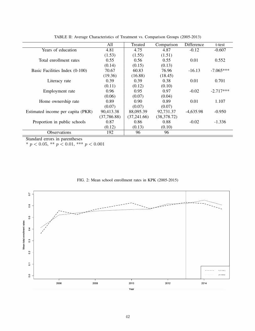
TABLE II: Average Characteristics of Treatment vs. Comparison Groups (2005-2013)

All Treated Comparison Difference t-testYears of education 4.81 4.75 4.87 -0.12 -0.607

(1.53) (1.55) (1.51)Total enrollment rates 0.55 0.56 0.55 0.01 0.552

(0.14) (0.15) (0.13)Basic Facilities Index (0-100) 70.67 60.83 76.96 -16.13 -7.065***

(19.36) (16.88) (18.45)Literacy rate 0.39 0.39 0.38 0.01 0.701

(0.11) (0.12) (0.10)Employment rate 0.96 0.95 0.97 -0.02 -2.717***

(0.06) (0.07) (0.04)Home ownership rate 0.89 0.90 0.89 0.01 1.107

(0.07) (0.07) (0.07)Estimated income per capita (PKR) 90,413.38 88,095.39 92,731.37 -4,635.98 -0.950

(37,786.88) (37,241.66) (38,378.72)Proportion in public schools 0.87 0.86 0.88 -0.02 -1.336

(0.12) (0.13) (0.10)Observations 192 96 96

Standard errors in parentheses* p < 0.05, ** p < 0.01, *** p < 0.001

FIG. 2: Mean school enrollment rates in KPK (2005-2015)

42

FIG. 3: Mean educational attainment in KPK (2005-2015)

FIG. 4: Mean school enrollment rates in KPK (2005-2015) for female respondents

43

FIG. 5: Mean educational attainment in KPK (2005-2015) for female respondents

TABLE III: Impact of Differential Investment on Educational Outcomes

(1a) (1b) (2a) (2b)Years of education Years of education Enrollment Enrollment

Treated 0.128*** -0.399* 0.247*** 0.192***(0.0177) (0.155) (0.00557) (0.0318)

Post 2013 -1.722*** -1.996*** 0.220** 0.0936(0.207) (0.317) (0.0680) (0.0843)

Treated x Post 2013 -0.227* -0.124 -0.0382 -0.0299(0.0887) (0.113) (0.0278) (0.0258)

Literacy rate 1.794** 0.134(0.626) (0.134)

Home ownership rate -0.960 0.0288(0.918) (0.158)

Employment rate 0.364 0.114(1.272) (0.0981)

Income per capita (PKR) 0.000000604 0.000000921***(0.00000225) (0.000000242)

Constant 6.139*** 6.224*** 0.281*** 0.0846(0.180) (1.315) (0.0513) (0.168)

N 240 240 240 240Standard errors in parentheses* p < 0.05, ** p < 0.01, *** p < 0.001

44

TABLE IV: Differential Investment on Educational Outcomes of Female Respondents

(3a) (3b) (4a) (4b)Years of education Years of education Enrollment Enrollment

Treated 0.506*** -0.296 0.319*** 0.254***(0.0294) (0.201) (0.00723) (0.0411)

Post 2013 -2.247*** -2.857*** -0.0347 -0.180(0.269) (0.388) (0.0872) (0.103)

Treated x Post 2013 -0.370* -0.209 -0.0648 -0.0555(0.147) (0.173) (0.0362) (0.0334)

Literacy rate 2.726** 0.155(0.791) (0.172)

Home ownership rate -0.485 -0.00434(0.981) (0.210)

Employment rate 0.792 0.150(1.209) (0.149)

Income per capita (PKR) 0.00000245 0.00000106**(0.00000293) (0.000000318)

Constant 6.145*** 5.107*** 0.401*** 0.191(0.211) (1.281) (0.0662) (0.216)

N 240 240 240 240Standard errors in parentheses* p < 0.05, ** p < 0.01, *** p < 0.001

45

Documents

Stanford Undergraduate Economics Journal Spring 2020 Volume 8