1

The Regional Economics Applications Laboratory (REAL) is a unit in the University of Illinois focusing on the development and use of analytical models for urban and region economic development. The purpose of the Discussion Papers is to circulate intermediate and final results of this research among readers within and outside REAL. The opinions and conclusions expressed in the papers are those of the authors and do not necessarily represent those of the University of Illinois. All requests and comments should be directed to Geoffrey J.D. Hewings, Director, Regional Economics Applications Laboratory, 607 South Mathews, Urbana, IL, 61801-3671, phone (217) 333-4740, FAX (217) 244-9339. Web page: www.real.illinois.edu/

The Economic Impact of a New Solar Power Plant in Arizona: Comparing

the Input-Output Results generated by JEDI vs. IMPLAN

Jinwon Bae and Sandy Dall’erba

REAL 15-T-5 August, 2015

2

The Economic Impact of a New Solar Power Plant in Arizona:

Comparing the Input-Output Results generated by JEDI vs.

IMPLAN

Jinwon Baea and Sandy Dall’erba

b,

a Regional Economics And Spatial Modeling laboratory and School of Geography and Development, University of

Arizona (email: jbae@arizona.email.edu)

b Department of Agricultural and Consumer Economics and Regional Economics Applications Laboratory,

University of Illinois at Urbana-Champaign (email: dallerba@illinois.edu)

Abstract.

As an increasingly adopted renewable energy resource, solar power has a high potential for

carbon emission reduction and economic development. This paper calculates the impact on job,

income and output creation of a new solar power plant in an input-output framework. The

contribution is twofold. First, we compare the multipliers generated by the construction and

operation/maintenance of a plant located in California with those it would have generated had it

been built in Arizona. Second, we point out the differences in the results obtained with the

popular IMPLAN software from those we get with the solar photovoltaic model of JEDI.

JEL Classification: R11, R15, Q42

Key words: Input-output, JEDI, IMPLAN, Solar photovoltaics

3

1 Introduction

Solar energy is increasingly seen as a major source of carbon emission and water consumption

reduction and its potential on human health and air quality has already been demonstrated

(Hernandez et al., 2014). Part of its growing success is technological progress that has allowed

the average price of solar silicon photovoltaic modules to drastically decrease from 65 USD/Watt

in 1976 to 1.4USD/Watt in 2010 (IPCC, 2014). The United States has arguably been a major

player in this trend. As one of the largest emitters of greenhouse gas1, the US has promoted the

deployment of low-carbon energy resources over the most recent decades (Storms et al., 2013).

For instance, more than 3.1 Gigawatts (GWs) of solar electricity generation facilities were

installed in the US in 2012 (Lacey et al., 2013). It elevated the accumulated amount of solar

photovoltaic facilities from 0.7% of the total renewable sources in the US in 2012 to 1.6% in

2013 (EIA 2013). These efforts are necessary to reduce GHG emissions because the energy

supply sector was responsible for almost a half (47%) of the increase in anthropogenic GHG

emissions between 2000 and 2010, while the industry sector produced around 30% of them

(IPCC, 2014).

Beyond the environmental benefits they generate, new solar power plants can also be seen as

a facility of which construction and operation will stimulate the local economy. There is an

increasing number of studies that compare the socio-economic impacts of multiple renewable

energy sources (Hillebrand et al., 2006; Lehr et al. 2008; Huntington, 2009; Pollin et al., 2009;

Carly et al., 2011; Tourkolias & Mirasgedis, 2011; Carley et al., 2012; De Arce et al., 2012;

Lambert & Silva, 2012; Lehr et al., 2012; Markaki et al., 2013) including solar energy. Most of

the latter studies are conducted in European countries, but increasing interest for renewable

1 6,135.03 MtCO2 (i.e. 13.5% of the world’s total) were emitted by the U.S. in 2011. It is the largest emitter after

China (10,260.32 MtCO2). However, in per capita terms, China produces 7.63 while the US produces 19.69 (WRI

2014).

4

energy in the US has led to several contributions in this country too over the last few years

(Huntington, 2009; Pollin et al., 2009; Carly et al., 2011; Carly et al., 2012). The large majority

of these studies conclude that a large impact on job and income creation takes place in the

economy of the area receiving the renewable energy facility, although its magnitude may be

smaller than the one generated by the traditional construction industry (Huntington, 2009).

As a leading source of RES, solar energy has led to a handful of economic impact analyses in

the US (Schwer & Riddle, 2004; Frisvold et al. 2009; Evans & James, 2011; Hamilton &

Berkman, 2011) as well as outside of the US (Cladés et al., 2009; Del Sol and Sauma, 2013).

Among the US-focused studies, all the applications are performed on either Nevada (Schwer &

Riddle, 2004), California (Hamilton & Berkman, 2011) or Arizona (Frisvold et al. 2009; Evans

& James, 2011) due to the large number of sunny days they experience each year.

The latter two states are the focus of this paper. Arizona ranks second only to California in

terms of solar energy generating potential in the country. Most areas in the state record more

than 6.0 kwh/m2/day of solar radiation which is among the highest levels in the nation (NREL,

2011). Yet, many feel the solar potential of the state has been barely tapped. The solar electric

capacity of Arizona was 1.8% of the state’s total electric capacity in 2013 (EIA, 2015 a) and

represents a cumulative capacity of 1093.5 MWs (Megawatts) according to Lacey et al. (2013).

In addition, in 2003 Arizona’s state legislature set the goal that 15% of its electricity would come

from renewable sources by 2025 (EIA, 2013) and at least 30% of them should come from

distributed generation (DSIRE, 2014). Furthermore, up to 70% of the distributed generation

could come from utility scale generation.

In order to examine further what would the economic impact of a new solar power plant in

Arizona be, this paper provides an input-output (I/O) analysis applied to the characteristics of the

5

Topaz Solar Farm, a 550MW facility built in California over Nov.2011-Nov.2013 and running at

full capacity since then2. It is an interesting case study in that it is the world’s largest solar farm

and its utility scale generation is expected to grow more than commercial and residential solar

panels. Indeed, it can improve cell grid reliability and stability and it already provides a

predictable and affordable source of energy to utility customers (FirstSolar, 2014). According to

Tucson Electric Power (TEP), the current unit cost per utility scale systems is as low as one-third

of rooftop systems (Hughes, 2013).

In this paper, our analysis calculates the jobs, income and output multipliers that would be

generated by a similar farm installed in Arizona and compares them with those that were

generated in California, in the counties of San Luis Obispo and Kern that host it, according to the

impact study produced by Hamilton (2011). This approach allows us to identify which of the two

regions has a competitive advantage in terms of economic multipliers. Furthermore, the 550 MW

case analyzed here can be seen as a benchmark against which the impact of future Arizona solar

farms can be estimated. The second objective of this paper is to compare the returns generated by

two different input-output software. The first one is IMPLAN (IMpact analysis for PLANning),

the leading model for economic impact analysis, and the second one is JEDI (Job and Economic

Development Impact model), a free and more recent model developed by NREL for the sole

purpose of measuring the economic impact of power generation and biofuel plants.

The rest of this paper is structured as follows: the next section provides a review of the input-

output literature applied to solar power generation as well as a description of the differences in

the two software used for the analysis. Section 3 reports the details of the investments associated

2 According to EIA, Topaz Solar Farm has been generating utility scale electricity since Feb. 2013 (239 MWh of net

generation) and the annual net generation was 1,053,373 MWh in 2014 (EIA, 2015 b), which corresponds to 121.9

MW. This amount is exactly 22.1% of 550MW installation and matches with the average annual system capacity of

utility scale in Table 1.

6

to the Topaz Solar Farm for both the construction and the operation/maintenance phases as they

are used as final demand change in the I/O model that comes in Section 4. This section shows the

direct, indirect and induced effects that result from such investments in California and in Arizona

according to both JEDI and IMPLAN. The effects are measured on job creation, labor income

and output change. While the results the two software generate are comparable, some

discrepancies are found and explained in this section. Finally, section 5 sums up the results and

provides some concluding remarks.

2 Literature Review and Basics of JEDI vs. IMPLAN

2.1 Input-output applied to solar energy production

Pioneered by Leontief in the late 1930s, input-output analysis examines the effects of a change in

final demand on the local economy. It relies on input-output tables that capture the market

transactions between the selling sectors (the providers) and the purchasing sectors or final

demand (the consumers). One of the advantages of input-output analysis is that it offers the

capacity to measure overall changes to the economy due to intersectoral (supply and purchase)

linkages (Miller and Blair, 2009), so that increasing demand for solar power in a locality will

lead to changes in demand in a large number of additional sectors which are not necessarily

directly related to electricity production. More precisely, a new solar farm creates a direct impact

in the construction sector (for the foundation, erection, electrical system of the project) and in the

services sector (for the permits, insurance) among others. It leads to an indirect impact when the

latter sectors purchase inputs, such as concrete and electric wires, necessary to support their own

activity. It also leads to an induced impact when the increased earnings generated in the previous

7

sectors are spent on local goods and services, such as food and education. In an I/O framework,

the sum of the direct, indirect and induced impacts constitutes the economic multipliers.

Based on this comprehensive framework, input-output analysis has been widely used to

measure the economic impact of various renewable energy sources and compare their relative

return. Their overall conclusion is that solar photovoltaics (PV) production provides larger

returns than other renewable energy sources per unit of production but not per dollar of

investment. For instance, Huntington (2009) finds that each MW of PV is between 4 and 11

times more effective than a MW of wind, biomass and natural gas at creating jobs in the US.

However, wind and biomass are more effective than PV when measured in dollar amount of

initial investment due to their lesser capital cost. Other studies do not provide both types of

relative returns but confirm this difference. For instance, Tourkolias and Mirasgedis (2011) use

an integrated approach to quantify the employment benefits of renewable energy resources in the

Greek economy in 2005. They find that it created an average of 265 job years/TWh for

geothermal during 35 years of lifetime, and 1503 job years/TWh for solar photovoltaics (PV)

during 20 years of lifetime. Moreno and Lopez (2008) conclude that in Spain the average job

creation per MW installed is 37.3 for solar PV, 31 for biogas, 20 for hydro, and 13.2 for wind.

On the other hand, Pollin et al. (2009) find that every $ one million of investment in biomass

energy production creates more jobs (17.4) than investments in solar (13.7) or wind (13.3) in the

US, thus confirming Huntington’s (2009) ranking based on cost.

Previous studies compare the returns of different renewable energy sources because they rely

on facilities located anywhere within a country and provide national-level impact estimates.

However, we focus in this paper on one type of facility only and it is located in a specific region.

The literature offers several regional I/O models applied to renewable energy sources. Among

8

the ones that focus on solar energy, we find Schwer and Riddle (2004) who report an

employment multiplier of 2.9 following the creation of a 100 megawatt (MWe) facility in

Nevada (2004- 2006). They found that the employment impacts are significantly less during the

O/M phase (2007 to 2035), but employment multiplier is about 3.1 because of relatively larger

indirect and induced impacts. Their work relies on the REMI model, a multivariate, multi-

equation model of the Nevada economy developed by the Regional Economic Models Inc.

Hamilton and Berkman (2011) start their input-output analysis by aggregating IMPLAN’s

440 economic sectors to a scheme that matches JEDI solar PV model. Their model is applied to a

solar farm in California and constitutes the benchmark against which our results on Arizona will

be compared. More details about their work appear in the next section. Another example is

Frisvold et al. (2009) who analyze the economic impact of the solar market growth in Arizona.

The state legislature is committed to have solar generation gradually increase from 32,300 MWh

in 2010 to 1.2 million kWh in 2025. A drop to 9,544,100 MWh in 2030 is also expected by the

authors because the share of renewable energy required in 2025 will have already been satisfied.

In their work, estimates on the future cost of energy, annual cash flow of solar technologies,

capital cost, payback and net present value are generated by Sandia National Laboratory in

collaboration with NREL. Based on this information, they use IMPLAN to quantify that opening

the needed solar power plants should have large economic and environmental benefits for the

state: the cumulative amount of new jobs is 277,759 during the construction period and 1,198 for

the O/M period corresponding to an employment multiplier of 1.95 and 1.48 respectively.

2.2 JEDI vs. IMPLAN

9

IMPLAN is one of the most-widely used tool for input-output analysis. It provides an extensive,

annually-updated data set dating back to 1977 (LLC, 2013). The version of IMPLAN we rely on

in this paper is 3.0 and the transactions among the 440 industrial sectors it encompasses are

measured in 2010. In contrast, JEDI is a free software that has been specifically designed by the

National Renewable Energy Laboratory (NREL) for analyzing the economic impact of new

renewable energy facilities. It offers the user to develop a model for 9 types of renewable energy

sources: Wind, Biofuels, Solar, Natural Gas, Coal, Marine/hydrokinetic Power, Geothermal,

Petroleum and Transmission Line Model. The solar model of interest to us allows the user to

distribute the electricity generated by residential, commercial and utility consumers. Additional

choices include the concentrated solar panel trough, the project photovoltaics and the scenario

photovoltaics (PV) in addition to user-input on the solar cell/module material, the average system

size, and the specified installation costs per materials and equipment vs. labor. Furthermore,

JEDI offers the possibility to separate the impact generated by the construction phase from that

due to the O/M phase.

The multipliers that JEDI generate are calculated at the state level3 and rely on IMPLAN’s

input-output tables. However, JEDI claims that the direct input coefficients have been modified

to reflect the actual intersectoral purchases made by the renewable energy sectors. These are

derived from extensive interviews JEDI has conducted with industry experts and professionals

alike (NREL, 2013). Another example of the specialization of JEDI is the limit on the average

annual system capacity to a value between 18.9-22.1%. It reflects that a solar power plant only

operates when the sun shines. By comparison, a coal power plant generally operates 80% of the

time (Wei et al., 2010). Table 1 below reports some of the attributes of JEDI these interviews and

3 Analysis of a specific region other than the state level can be only performed through the “User Add-in Location”

feature in JEDI that requires inputting local multipliers and other necessary information.

10

experience with the renewable energy sectors have led to. JEDI still offers the users the capacity

to modify the default values below, but we decide to keep them in this study. In contrast,

IMPLAN does not have a sector that is specifically for power plants, so that the “construction”

sector (NAICS 34-38) and the “maintenance” sector (NAICS 39) are the ones that will be used in

the rest of the analysis by IMPLAN.

Table 1. Defaults in JEDI solar PV by energy use

residential

retrofit

residential new

construction

small

commercial

large

commercial

Utility

Average annual system capacity

factor (percentage):

18.9% 18.9% 18.9% 20.4% 22.1%

Average system size– Direct

Current Nameplate Capacity (kW)

5.7 3.5 20 150 1000

Annual direct O/M cost ($/kW) < $25.22 < $25.22 < $20.25 < $18.34 < $17.84

It is important to note that, in spite of its many useful features, JEDI presents the same

shortcomings as any other input-output model such as the lack of consideration for

“technological improvements, import substitution, changes in consumption patterns, or relative

price variations over time” (Lambert and Silva, 2012, p.4668)

3. Topaz Solar Farm, our 550 MW Case study

In the absence of data specific to an existing or planned solar plant in Arizona, this study uses the

features of the Topaz Solar Farm (TSF) that was built in 2013 in San Luis Obispo County,

California. It was constructed for 3500 acres of utility-scale solar farming with a proposed

photovoltaic capacity of 550 MW. It provides power for 160,000 average homes and meets 65%

of the 1.7GWh of energy annually consumed in San Luis Obispo County. The cost of the plant is

as follows: $ 175 million are spent during the three years of the construction period (2011-2013)

whereas $ 2.475 million are expected to be spent annually during the next 25 years for the plant’s

11

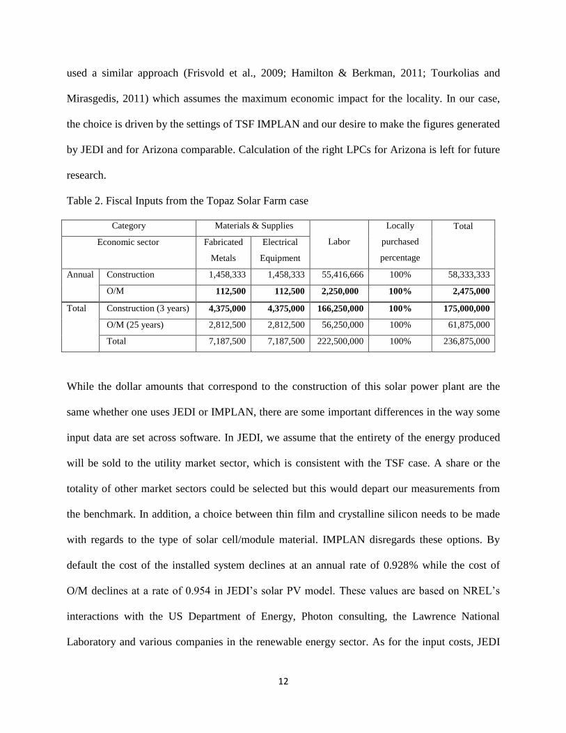
operation and maintenance ($ 61.875 million in total). All costs are for labor, materials and

supplies. In addition, it is assumed during the operating period that the spending on material and

supplies is 10% of the spending on labor. Another assumption is that the modules/inverters are

imported from outside the county. All the above figures are in 2011 dollar value and a discount

rate of 2% is used to actualize future revenues. The economic impact analysis of TSF that we use

as a benchmark in this paper was performed by Hamilton and Berkman (2011) using IMPLAN

v3. The impact they calculate takes place over two neighboring counties, San Luis Obispo and

Kern county, that constitute the area where the solar energy is sold and from which the workers

are drawn. The model assumes that at least 60% of the money is spent in the former county.

The impacts and multipliers estimated by Hamilton and Berkman (2011) will be discussed

throughout the rest of this paper and will be compared with the impacts of a similar investment

in the state of Arizona. However, several adjustments are necessary to apply the figures of TSF

to JEDI. First, all the dollar values are expressed in 2012 because it is the first year for which the

IO model can run in our version of JEDI. They appear in table 2 below. The 3-year construction

period is thus 2012-2014 and the following 25 years of O/M cover 2015-2039. Since both

IMPLAN and the JEDI solar PV model can estimate returns until 2030 only (i.e. 16 years of

O/M) we extend the O/M period by adopting an annual depreciation rate of 1.257% for 2030-

2039. It corresponds to the rate observed over the last three years (2027-2030). In that situation,

the spending for O/M increases from $39.6 million to $61.875 million in 2012 dollar. Finally, we

assume that the modules and inverter are not locally purchased, just like in the TSF case4.

Therefore, the models in this study estimates the maximum impacts on the local economy by

assuming all the inputs (materials, equipment and labor) are supplied locally. Many studies have

4 It should be noted that the local purchase percentages (LPC) of fabricated metals and electrical equipment

4 are

26.54% and 7.70% respectively based on the SAM model values found in the Arizona 2010 IMPLAN dataset during

the whole period of construction and O/M

12

used a similar approach (Frisvold et al., 2009; Hamilton & Berkman, 2011; Tourkolias and

Mirasgedis, 2011) which assumes the maximum economic impact for the locality. In our case,

the choice is driven by the settings of TSF IMPLAN and our desire to make the figures generated

by JEDI and for Arizona comparable. Calculation of the right LPCs for Arizona is left for future

research.

Table 2. Fiscal Inputs from the Topaz Solar Farm case

Category Materials & Supplies

Labor

Locally

purchased

percentage

Total

Economic sector Fabricated

Metals

Electrical

Equipment

Annual Construction 1,458,333 1,458,333 55,416,666 100% 58,333,333

O/M 112,500 112,500 2,250,000 100% 2,475,000

Total Construction (3 years) 4,375,000 4,375,000 166,250,000 100% 175,000,000

O/M (25 years) 2,812,500 2,812,500 56,250,000 100% 61,875,000

Total 7,187,500 7,187,500 222,500,000 100% 236,875,000

While the dollar amounts that correspond to the construction of this solar power plant are the

same whether one uses JEDI or IMPLAN, there are some important differences in the way some

input data are set across software. In JEDI, we assume that the entirety of the energy produced

will be sold to the utility market sector, which is consistent with the TSF case. A share or the

totality of other market sectors could be selected but this would depart our measurements from

the benchmark. In addition, a choice between thin film and crystalline silicon needs to be made

with regards to the type of solar cell/module material. IMPLAN disregards these options. By

default the cost of the installed system declines at an annual rate of 0.928% while the cost of

O/M declines at a rate of 0.954 in JEDI’s solar PV model. These values are based on NREL’s

interactions with the US Department of Energy, Photon consulting, the Lawrence National

Laboratory and various companies in the renewable energy sector. As for the input costs, JEDI

13

offers a preset allocation by expenditure type that we adjust to reflect TSF’s scenario. More

precisely, we allocate 10% of the labor cost to mounting and electrical equipment each year. By

default JEDI allocates 27.7% of the total costs to the category “other costs” which encompasses

permitting (1.7%), business overhead (20.6%) and other miscellaneous costs (5.4%). Changing

these inputs manually affects the role of ‘professional services’ and ‘other services' in the final

economic impact. Therefore, we modify the allocation of the installation costs to match our case

study and keep the default value of ‘other costs’ in JEDI. Then the rest (72.3%) is allocated for

labor (68.7%), mounting (1.8%), and electrical equipment (1.8%)

In order to guarantee the primary data in IMPLAN match the ones of JEDI, we aggregate the

economic sectors of IMPLAN based on the sectoral scheme used by NREL (2008) for the solar

industry so that construction, electric services and the manufacturing sectors are subdivided into

detailed sectors whereas other sectors are aggregated at a higher level in JEDI. As a result, the

440 industries of IMPLAN are aggregated into the following 22 sectors: 1) Agriculture, Forestry,

Fish & Hunting, 2) Mining, 3) Construction, 4) Construction/Installations - Non Residential, 5)

Construction/Installation Residential, 6) Manufacturing, 7) Fabricated Metals, 8) Machinery, 9)

Electrical Equip, 10) Battery Manufacturing, 11) Energy Wire Manufacturing, 12) Wholesale

Trade, 13) Retail trade, 14) TCPU, 15) Insurance and Real Estate, 16) Finance, 17) Other

Professional Services, 18) Office Services, 19) Architectural and Engineering Services, 20)

Other services, 21) Government, and 22) Semiconductor (solar cell/module) manufacturing.

Note that the “Electric power generation, solar” sector, which is associated to O/M of a solar

farm belongs to “Other services” (sector 20) according to the North American Industry

Classification System (NAICS) classification (see Appendix I).

14

4. Results

Table 3 reports the results of the four models under study: 1) those calculated for TSF by

Hamilton and Berkman (2010) with IMPLAN; 2) those we generate for California with the JEDI

model; while 3) and 4) are the results we obtain for Arizona based on IMPLAN and JEDI

respectively. Our calculations indicate, first, that all four cases lead to roughly the same number

of total jobs and total output created by the end of the project. The total number of job years

created ranges from 11.56 to 11.84 per $ million of investment. These results are slightly lower

than those found in Pollin et al.’s (13.7), but higher than those of Huntington (7.80 for 20%

capacity and 11.12 for 80% capacity). In this paper, we rely on an annual capacity of 22.1% in

the JEDI models, which is the default value for utility scale. All models indicate also that more

than 80% of the job years created take place during the construction period. The total outputs are

estimated to be $1.76-1.78 million in California and $ 1.54-1.57 million in Arizona for every

$ one million of spending. Overall, the installation of a solar farm in Arizona would create less

labor income and output than in California with the bulk of the difference coming from the

construction phase.

The largest source of the difference between JEDI and IMPLAN can be seen in the changes

in labor income. JEDI calculates a lower direct impact in both the CA and AZ cases. This

difference propagates to the indirect and induced effects, although in Arizona they are relatively

greater in IMPLAN than in JEDI per unit of direct effect. As a result, the overall income created

is nearly twice as large in JEDI than in IMPLAN. The difference could come from JEDI

allocating 27.7% of spending to high value-added activities such as permitting, business

overhead and “other services” by default. In contrast, IMPLAN does not reveal the direct input

coefficients allocated to any of the previous three activities. Another source of the difference

15

with the benchmark is that labor in the direct sectors is cheaper in Arizona than in California.

Indeed, the mean annual wage of solar photovoltaic installers is $35,760 in Arizona, i.e. $ 7,520

less than in California as of May 2014 (USDOL, 2014).

Table 3. Economic impacts of TSF / $ one million of spending

Local economic

impacts

TSF IMPLAN model – benchmark California JEDI model

Job

years5

Labor

Income ($)

Output

($)

Job

years

Labor

Income ($)

Output

($)

Construction

Direct Effect 5.07 710,593.72 738,786.28 4.33 571,577.63 613,311.23

Indirect Effect 0.95 51,716.64 161,763.78 2.29 149,990.75 408,000.45

Induced Effect 3.15 156,735.32 467,436.65 3.31 181,984.13 514,914.85

Construction total 9.17 919,045.69 1,367,986.71 9.93 903,552.52 1,536,226.53

O/M

Direct Effect 1.58 99,971.48 261,213.72 0.99 135,965.93 135,965.93

Indirect Effect 0.33 18,238.72 57,227.29 0.26 16,981.29 49,064.72

Induced Effect 0.49 24,302.67 72,452.80 0.40 22,918.03 64,830.89

O/M total 2.41 142,512.87 390,893.80 1.65 175,865.39 249,861.66

Total Effect 11.57 1,061,558.56 1,758,880.52 11.59 1,079,417.91 1,786,088.19

Arizona IMPLAN model Arizona JEDI model

Job

years

Labor

Income ($)

Output

($)

Job

years

Labor

Income ($)

Output

($)

Construction

Direct Effect 4.79 240,873.39 682,285.56 4.64 571,372.90 613,311.23

Indirect Effect 1.81 93,833.34 230,254.72 2.43 126,957.00 339,125.74

Induced Effect 2.68 112,264.25 328,105.36 3.11 137,546.30 388,390.92

Construction total 9.29 446,970.98 1,240,645.64 10.18 835,876.20 1,340,827.89

O/M

Direct Effect 1.22 62,777.89 171,501.80 0.99 136,045.66 136,045.66

Indirect Effect 0.39 20,694.61 50,636.14 0.27 13,504.26 41,230.62

Induced Effect 0.67 27,967.69 81,648.44 0.40 18,276.74 51,657.02

O/M total 2.28 111,440.73 303,786.40 1.66 167,826.66 228,933.30

Total Effect 11.56 558,411.71 1,544,432.04 11.84 1,003,702.86 1,569,761.18

Note: Dollar year value for all models is 2011.

The O/M period in the TSF JEDI, Arizona IMPLAN and JEDI models is extended to the year 2039 to match

the TSF case.

The difference with the Arizona JEDI model is much less obvious probably because the latter

is more familiar with the type of skills required in the renewable energy sector. For example, the

5 Job years refer to full time equivalent (FTE) employment for a year (1 FTE equals to 2080 hours)

16

mean annual wage of a construction worker is much lower ($30,470) than that of a solar

photovoltaic installers mentioned above (USDOL, 2014). However, by default JEDI sets the

labor cost to $450/kW during the construction period and to $10.70/kW during the O/M period in

Arizona or California.

On the other hand, the TSF models lead to a much greater labor income (about $ 1.08 million

per $ one million of spending) and output level (about $ 1.79 million per $ one million spending)

than the Arizona models. It is mainly due to the greater feedback in the indirect and induced

effects that emanate from the local economy of California. In addition, the California JEDI

model leads to more labor income and output than the California IMPLAN model. The larger

return is partially due to the difference in labor costs but also to the options specified in JEDI

such as the average annual system capacity factor, the procurement of materials and equipment,

the allocation by final consumers (residential, commercial and utility scale) and the solar

cell/module material. However, it is important to note that the difference is to be expected as the

California JEDI model is performed over the state as a whole while the TSF IMPLAN model is

for two counties only.

Table 4 reports the indirect and induced employment effects of a $ one million of investment

for each of our four models. The results appear for six sectors aggregated as in the sectoral

scheme available in JEDI. Unfortunately JEDI does not report the figures by sector for the O/M

period. All the models report an induced effect that is much larger than the indirect effect and

that most of the employment creation takes place during the construction period. In the TSF

IMPLAN model, the sector experiencing the largest indirect effect is ‘wholesale trade and retail’

(0.32) while ‘other services’ (1.61) experiences the largest induced effect – the bulk of it is

taking place during the construction period. On the other hand, the Arizona IMPLAN model

17

estimates the largest indirect and induced effect in ‘other services’ (0.59 and 1.34), again during

the construction period. For the JEDI models which rely on a different set of assumptions (see

section 2), the largest number of jobs created is in ‘other sectors’ and its value is more than 10

times the matching figure from IMPLAN (1.29 for TSF JEDI and 1.39 for Arizona JEDI).

Table 4. Employment effect by sectors based on spending of $ one million

Employment effect TSF IMPLAN California JEDI Arizona IMPLAN Arizona JEDI

Construction O/M Construction O/M Construction O/M Construction O/M

Indirect Effect 0.95 0.33 2.26 0.26 1.81 0.41 2.4 0.26

Manufacturing Impacts 0.04 0.01 0.19 0 0.08 0.02 0.20 -

Trade (Wholesale & Retail) 0.32 0.11 0.24 0 0.39 0.08 0.25 -

Finance, Insurance & Real Estate 0.08 0.03 0.00 - 0.15 0.03 0.00 -

Professional Services 0.23 0.08 0.14 - 0.50 0.11 0.16 -

Other Services 0.20 0.07 0.39 - 0.59 0.14 0.40 -

Other Sectors 0.07 0.02 1.29 - 0.11 0.03 1.39 -

Induced Effect 3.16 0.49 3.26 0.40 2.68 0.67 3.06 0.40

Manufacturing Impacts 0.03 0.00 - - 0.03 0.01 - -

Trade (Wholesale & Retail) 0.80 0.12 - - 0.58 0.15 - -

Finance, Insurance & Real Estate 0.50 0.08 - - 0.50 0.13 - -

Professional Services 0.11 0.02 - - 0.09 0.03 - -

Other Services 1.61 0.25 - - 1.34 0.33 - -

Other Sectors 0.11 0.02 - - 0.15 0.04 - -

‘-‘ means no information

We report in table 5 the multipliers that correspond to the figures displayed in table 3. We

focus on job, labor income and output type I and type SAM Multipliers. The difference between

the latter two is that Type I multipliers account for the indirect effects only whereas Type SAM

multipliers consider both indirect and induced effects. The multipliers range from 1.07 to 1.85 in

the TSF IMPLAN model, 1.12 to 2.50 in the California JEDI model, 1.32 to 1.94 in the Arizona

IMPLAN6 model and from 1.10 to 2.19 in the Arizona JEDI model. As a result and according to

JEDI, a new facility leads to a larger multiplier effect in terms of jobs, labor income and output

in California than in Arizona. They come from the comparatively larger indirect and induced

6 Our results by Arizona IMPLAN are in tune with those of Frisvold et al. (2009) as they find an employment

multiplier of 1.95 and 1.48 for the construction and O/M periods respectively.

18

effects as well as from the larger size of the study area (California is 1.4 and 5.7 times bigger and

more populated than Arizona). Comparison based on the two IMPLAN models is not appropriate

since they are not dealing with the same territory (two counties in CA vs. AZ as a whole).

Table 5. Multipliers of TSF and solar farm in Arizona based on spending

Multipliers TSF IMPLAN California JEDI

Job

years

Labor

Income

Output Job

years

Labor

Income

Output

Construction Type 1 1.19 1.07 1.22 1.53 1.26 1.67

Type SAM 1.81 1.29 1.85 2.29 1.58 2.50

O/M Type 1 1.21 1.18 1.22 1.26 1.12 1.36

Type SAM 1.53 1.43 1.50 1.67 1.29 1.84

Total Type 1 1.19 1.09 1.22 1.48 1.24 1.61

Type SAM 1.74 1.31 1.76 2.18 1.53 2.38

Multipliers Arizona IMPLAN Arizona JEDI

Job

years

Labor

Income

Output Job

years

Labor

Income

Output

Construction Type 1 1.38 1.39 1.34 1.52 1.22 1.55

Type SAM 1.94 1.86 1.82 2.19 1.46 2.19

O/M Type 1 1.32 1.33 1.30 1.27 1.10 1.30

Type SAM 1.87 1.78 1.77 1.68 1.23 1.68

Total Type 1 1.37 1.38 1.33 1.48 1.20 1.51

Type SAM 1.92 1.84 1.81 2.10 1.42 2.09

1) Type I Multiplier = (Direct Effect + Indirect Effect) / (Direct Effect)

2) Type SAM Multiplier= (Direct Effect + Indirect Effect + Induced Effect) / (Direct Effect)

5. Conclusion

The benefits of a new solar power plant with large utility scale go beyond the environmental

advantages of replacing fossil fuel energy sources with low carbon emission sources. New power

plants have a large impact on the economy of the area that hosts them. This paper focuses on

Arizona where solar radiation is abundant and takes place all year long. The economic impacts of

the world’s largest solar plant called Topaz recently built in California serves as a benchmark

against which we measure the impact of the same investment but in Arizona. In that purpose, we

19

use the popular IMPLAN model, as in the economic impact study performed by Hamilton (2001)

for the Topaz case, and compare the results it generates with those of the JEDI Solar module, a

free software developed by the NREL. It allows us to compare how the differences in the input

characteristics lead the two models to generate slightly different overall impacts. Indeed, while

IMPLAN provides detailed information about a very large number of sectors, it does not have a

sector specific to the construction of a solar plant. On the other hand, JEDI counts few sectors

but it is specifically designed for economic impact analyses of renewable energy facilities. It

offers a large set of options on the average annual system capacity factor, the procurement of

materials and equipment, the detailed market sector share (residential, commercial and utility

scale) and the solar cell/module material. Its creators claim that these options derive from

numerous interactions with companies in the renewable energy sector, the U.S. Department of

Energy, Photon consulting and Lawrence Berkeley National Laboratory.

One consequence of this difference is that during the construction period the direct labor

income is nearly twice larger in the JEDI Arizona model than in the IMPLAN Arizona model.

We believe that it is because IMPLAN uses the average income of a worker in the construction

sector no matter what type of facility is being built. Instead, JEDI accounts for the costs specific

to a solar plant and automatically allocates 27.4% of the construction costs to high value-added

sectors such as permitting and business overheads.

In spite of these differences, our economic impact analysis shows that all four models - TSF

IMPLAN, California JEDI, Arizona IMPLAN and Arizona JEDI model - generate reasonable

results that are fairly similar in terms of total job and output creation. For instance, all models

indicate that about 80% of the total job creation takes place during the construction period. In

addition, the total number of job years is similar at about 11.5 and the JEDI models calculate a

20

labor income multiplier (resp. output multiplier) that is only 1.08 times (resp. 1.14 times) larger

in California than in Arizona. The slightly greater overall return that California displays over

Arizona comes from its larger indirect and induced income effects. Indeed, the same of solar

photovoltaic installer would make $ 7,520 more a year in California than in Arizona (USDOL,

2014).

Our results indicate also that the JEDI solar PV model is very efficient at generating an

economic impact analysis by input-output. First of all, the input options available to the JEDI

user are very specific to the solar energy industry, which means that JEDI relies on direct input

coefficients that are more realistic. For example, the latter vary with the user’s choice of energy

use (residential, commercial, and utility) and cost per kW allocated to materials and equipment,

labor, permitting and business overhead. Second, the 22 industrial sectors integrated in JEDI

keep the sectors related to solar energy very detailed, while the others are aggregated. IMPLAN

will always have an advantage in terms of the number of industrial sectors it offers (440), but

JEDI’s aggregation scheme allows the user to focus on the most relevant sectors for his/her study.

These two advantages, combined with its free access, make JEDI a very appealing software for

economic impact analysts focusing on RES. One possible shortcoming of JEDI is its intrinsic

focus on state level analysis – because the transaction table it relies on is as such – but it can

easily be overcome by combining JEDI with a local I/O table from IMPLAN. In this case, the

direct job multipliers of the region of interest can be transferred from IMPLAN to JEDI using its

user add-in function. As for setting the appropriate LPC in JEDI, the SAM model values that are

offered in IMPLAN can help improve the accuracy of local estimates generated by JEDI.

In this paper, we have estimated the upper threshold of the local economic impact following

a new solar plant. Our choice was driven by the inputs used in the analysis of the TSF built in

21

California. However, we would like to investigate in the future whether a change in the LPCs

would affect our results. Another extension of interest for the state of Arizona consists in

investigating whether facilities built for other types of renewable energy sources, such as wind,

geothermal or biomass, could lead to greater multiplier effects on the economy. These results

could help state and local policy-makers justify their spending for more renewable energy

facilities and figure out their “right” mix based on their relative multipliers and the state’s current

and future natural resources endowment.

22

Appendix I. Industry Aggregation scheme of JEDI PV model

Aggregated JEDI industry name IMPLAN Industry code

Agriculture 1-19

Mining 20-30

Construction 34-38

Construction – Nonresidential 39

Construction – Residential 40

Other Manufacturing 41-185, 187-206, 208-221, 225-231, 234-

265, 267, 271, 274, 276-318

Fabricated Metals 186

Machinery 207, 222-224, 232-233

Electrical Equipment 266, 268-269, 273, 275

Battery Manufacturing 270

Energy Wiring Manufacturing 272

Semiconductor and related devices 243

Wholesale Trade 319

Retail Trade 320-331

Transportation, Communication, and Public Utilities 31-33, 332-335, 337

Finance 354-356

Insurance and Real Estate 357-361

Other Professional Services 367, 374-376, 381

Architectural and Engineering 369-370

Office Services 368

Other Services 336, 338-366, 371-373, 377-380, 382-426,

433-436

Government 427-432, 437-440

Edited from JEDI PV 2008 Industry Aggregation Scheme (PV model only), NREL.

23

References

Blanco, Maria Isabel and Glória Rodrigues 2009. Direct employment in the wind energy sector: An EU study.

Energy Policy 37: 2847-2857.

Caldes, N., Varela, M., Santamaria, M., & Saez, R. (2009). Economic impact of solar thermal electricity deployment

in Spain. Energy Policy, 37(5), 1628-1636.

Carley, S., Lawrence, S., Brown, A., Nourafshan, A., & Benami, E. (2011). Energy-based economic development.

Renewable and Sustainable Energy Reviews, 15(1), 282-295.

Carley, S., Brown, A., & Lawrence, S. (2012). Economic Development and Energy: From Fad to a Sustainable

Discipline? Economic Development Quarterly, 26(2), 111-123

De Arce, Rafael, Ramón Mahía, Eva Medina and Gonzalo Escribano 2012. A simulation of the economic impact of

renewable energy development in Morocco. Energy Policy 46: 335-345.

Del Sol, F., and Sauma, E. (2013). Economic impacts of installing solar power plants in northern Chile. Renewable

and Sustainable Energy Reviews, 19(0), 489-498.

DSIRE 2014. Renewable Energy Standard. In Renewable Energy Standard: Arizona Incentives/Policies for

Renewables & efficiency.

EIA 2013. Arizona State Profile and Energy Estimates. In Arizona State Profile and Energy Estimates: U.S. Energy

Information Administration.

EIA 2015 a. Electricity, Annual Data: Net Generation by State by Type of Producer by Energy Source (EIA-906,

EIA-920, and EIA-923) 1990-2013. Retrieved March 2015, from Energy Information Administration

http://www.eia.gov/electricity/data/state/

EIA 2015 b. Electric Power Monthly. In Electric Power Monthly: US Energy Information Administration. Retrieved

April 2015, from: http://www.eia.gov.

Evans, A., & James, T. (2011). Impact of Solar Generation upon Arizona's Energy (Electricity) Security: L. William

Seidman Research Institute W. P. Carey School of Business Arizona State University.

FirstSolar 2014. Utility-Scale Generation. In Utility-Scale Generation, First Solar: First Solar.

Friedman, B 2012. PV Installation Labor Market Analysis and PV JEDI Tool Developments (Presentation). In PV

Installation Labor Market Analysis and PV JEDI Tool Developments (Presentation): NREL (National

Renewable Energy Laboratory).

Frisvold, G., W. P. Patton and S. Raynold 2009. Arizona solar energy and economics outlook. Prepared for Arizona

Solar Energy and Economics Summit.

Giesken, Mark Louis 2007. Economic Impact of Wind Farm Development in Oklahoma. Department of Geography,

University of Oklahoma.

Hamilton, S. F. 2011. Economic and fiscal impacts of the Topaz Solar Farm. In Economic and fiscal impacts of the

Topaz Solar Farm: The Battle Group.

Hernandez, R. R., S. B. Easter, M. L. Murphy-Mariscal, F. T. Maestre, M. Tavassoli, E. B. Allen, C. W. Barrows, J.

Belnap, R. Ochoa-Hueso, S. Ravi and M. F. Allen 2014. Environmental impacts of utility-scale solar energy.

Renewable and Sustainable Energy Reviews 29: 766-779.

24

Hillebrand, Bernhard, Hans Georg Buttermann, Jean Marc Behringer and Michaela Bleuel 2006. The expansion of

renewable energies and employment effects in Germany. Energy Policy 34: 3484-3494.

Hughes, James A. 2013. Utilities right to seek most bang for their solar buck: Rules should be fair to all. In Utilities

right to seek most bang for their solar buck: Rules should be fair to all: AZ Central.

Huntington, H. G. (2009). Creating Jobs With ‘Green’ Power Sources. Paper presented at the Energy Modeling

Forum, Stanford.

IPCC, 2014: Summary for Policymakers, In: Climate Change 2014, Mitigation of Climate Change. Contribution of

Working Group III to the Fifth Assessment Report of the Intergovernmental Panel on Climate Change

[Edenhofer, O., R. Pichs-Madruga, Y. Sokona, E. Farahani, S. Kadner, K. Seyboth, A. Adler, I. Baum, S.

Brunner, P. Eickemeier, B. Kriemann, J. Savolainen, S. Schlomer, C. von Stechow, T. Zwickel and J.C. Minx

(eds.)]. Cambridge University Press, Cambridge, United Kingdom and New York, NY, USA.

Kammen, Daniel M., Kamal Kapadia, and Matthias Fripp (2004). “Putting Renewables to Work: How Many Jobs

Can the Clean Energy Industry Generate?” RAEL Report, University of California, Berkeley.

Lacey, S., H. Trabish and E. Wesoff 2013. Potraits of a manufacturing solar market : How key states are fairing. In

Potraits of a manufacturing solar market : How key states are fairing: Greentechmedia.com.

Lambert, Rosebud Jasmine and Patrícia Pereira Silva 2012. The challenges of determining the employment effects

of renewable energy. Renewable and Sustainable Energy Reviews 16: 4667-4674.

Lehr, Ulrike, Joachim Nitsch, Marlene Kratzat, Christian Lutz and Dietmar Edler 2008. Renewable energy and

employment in Germany. Energy Policy 36: 108-117.

LLC, IMPLAN Group 2013. About IMPLAN. In About IMPLAN.

Lorca, Alejandro and Rafael De Arce 2012. Renewable energies and sustainable development in the Mediterranean:

Morocco and the Mediterranean solar plant. Forum Euroméditerranéen des Instituts de Sciences Économiques.

Markaki, M., A. Belegri-Roboli, P. Michaelides, S. Mirasgedis and D. P. Lalas 2013. The impact of clean energy

investments on the Greek economy: An input–output analysis (2010–2020). Energy Policy 57: 263-275.

Miller, R. E. and P. D. Blair, 2009. Input-Output Analysis: Foundations and Extensions, 2nd

Edition.

Moreno, B., & López, A. J. (2008). The effect of renewable energy on employment. The case of Asturias (Spain).

Renewable and Sustainable Energy Reviews, 12(3), 732-751.

Mulligan, Gordon, Randall Jackson and Amanda Krugh 2013. Economic base multipliers: a comparison of ACDS

and IMPLAN. Regional Science Policy & Practice 5: 289-303.

NREL 2008. JEDI PV industry aggregation scheme. In JEDI PV industry aggregation scheme.

NREL 2011. Dynamic Maps, GIS Data, & Analysis Tools: Lower 48 PV 10km Resolution 1998 to 2005. Retrieved

11/20/2014, from NREL http://www.nrel.gov/gis/data_solar.html

NREL 2013. JEDI - Jobs and Economic Development Impact Models. In JEDI - Jobs and Economic Development

Impact Models: National Renewable Energy Laboratory.

Pollin, R., James Heintz, & Garrett-Peltier, H. (2009). The Economic Benefits of Investing in Clean Energy:

Department of Economics and Political Economy Research Institute (PERI) & Center For American Progress.

25

Schwer, R. K. and M. Riddel 2004. The Potential Economic Impact of Constructing and Operating Solar Power

Generation Facilities in Nevada. In The Potential Economic Impact of Constructing and Operating Solar

Power Generation Facilities in Nevada: NREL.

SEIA 2014. Solar Market Insight Report 2014 Q1. In Solar Market Insight Report 2014 Q1.

Storms, D., S. L. Dashiell and F. David 2013. Siting solar energy development to minimize biological impacts.

Renewable Energy 57: 289-298.

Tourkolias, C. and S. Mirasgedis 2011. Quantification and monetization of employment benefits associated with

renewable energy technologies in Greece. Renewable and Sustainable Energy Reviews 15: 2876-2886.

US DOL (United States Department of Labor) (2014). Occupational Employment Statistics. May 2015, from

http://www.bls.gov/oes/current/oes_az.htm#47-0000

Wei, Max, Shana Patadia and Daniel M. Kammen 2010. Putting renewables and energy efficiency to work: How

many jobs can the clean energy industry generate in the US? Energy Policy 38: 919-931.

Williams, Susan K., Tom Acker, Marshall Goldberg and Megan Greve 2008. Estimating the economic benefits of

wind energy projects using Monte Carlo simulation with economic input/output analysis. Wind Energy 11:

397-414.

WRI 2014. CAIT 2.0, WRI's Climate Data Explorer. In CAIT 2.0, WRI's Climate Data Explorer, CAIT 2.0.