Embed Size (px)
Citation preview
.'
Project 81307 No. 29August 1986
THE ECONOMETRICS OFMODELS WITH RATIONAL EXPECTATIONS
Benny Lee
,
CONTENTS
Summary
1. Introduction
2. Non-rational Expectation Models in Economics
3. The Rational Expectations Hypothesis
3.1 Properties of Muthian rationality3.2 Applications of rational expectations in economics
4. Statistical Identification
4.1 Models with current expectations4.2 Models with future expectations and other
complications
5. Estimation Problems
6. Hypothesis Testing
7. The Lucas Critique of Conventional EconometricPolicy Evalu~tion
8. Conclusion
References
THE ECONOMETRICS OF MODELS WITH RATIONAL EXPECTATIONS
Benny Lee
SUMMARY
Muth's (1961) paper has triggered off the so-called Rational Expectations
revolution in economics research. The rational expectations approach in
modelling economic behaviour has the merit of formalising expectations
according to coherent economic principles rather than ad hoc assumptions
such as those which extrapolate from the past. The hypothesis that
expectations and model structure are interdependent has, however, posed
serious problems for econometricians attempting to identify, estimate,
test and simulate models with rational expectations. Furthermore, it may
not in general be possible to infer empirically whether it is the model
structure or.the rationality hypothesis that has been refuted by the data.
This paper is a review of various econometric problems associated with
models employing rational expectations, with a discussion of possible ways
of overcoming them.
Helpful comments from Brian Fisher, John Spriggs, Steve Beare and other
colleagues at BAE are gratefully acknowledged. The author is, however,
responsible for any error that remains.
1
1. INTRODUCTION
Economics is concerned with human behaviour reacting to both current and
anticipated events. Rational economic decisions are made under conditions
w~ich are partly unknown to the decision makers. In econometric models,
anticipated events are usually represented in the form of unobservable
expectations variables. While it may be convenient to leave the nature of
expectations formation vague when developing economic theories,
quantitative policy evaluation and forecasting have to be based on exact
representation of the expectation variables. This connection becomes more
critical as conflicting forecasts are produced by econometric models using
different expectations assumptions. A notable example is the debate on the
effectiveness of countercyclical policy in the macroeconomics literature
(Sargent and Wallace 1976; Lucas and Sargent 1978).
Before the introduction of Muth's (1961) rational expectations
hypothesis, econometricians made ad hoc assumptions and used simple proxy
variables to replace the unobservable expectations variables in their
econometric models. These proxies could be data from futures markets,
sample surveys, predictions from time series models, econometric model
forecasts and/or the actual values (assuming perfect foresight). With the
introduction of the rational expectation hypothesis, econometricians can
now integrate the specification of both model structure and expectations
formation. One result is to complicate the identification and estimation
of the model. The conventional tool-kit, which originated from the Cowles
Commission (Fisher 1966) and emphasises exclusion restrictions (for
example, that, to distinguish a demand equation from a supply equation,
certain variables should occur in one of the equations), is no longer
adequate.
The object of this paper is to bring together the various
contributions in the literature and to make them more accessible to
economists who wish to familiarise .themselves with the topic. In
section 2, non-rational expectation approaches in economics are reviewed.
Section 3 is a recapitulation of the concept of rational expectations and
of· its manifestations in dif~erent contexts. Sections 4 and 5,
respectively, deal with the identification problem of models with rational
expectations and the problem of estimating these models. In sections 6
2
and 7, respectively, problems of hypothesis testing and policy evaluation
are discussed. ConcluSions and directions for further research are given
in section 8.
2. NON-RATIONAL EXPECTATION MODELS IN ECONOMICS
Expectations, in economics, are essentially forecasts of the future values
of economic variables. It should be noted that, being the personal
judgments of particular individuals, they are essentially subjective.
Usually, an expectation should better be characterised by a probability
distribution than by a single predicted value. However, provided that the
models are linear and stochastic, there is no loss of generality in
summarising the expectation by the mean of the distribution.
Keynes (1936, p.47) stressed that expectations playa major role in
influencing economic decisions. While accepting that expectations are
likely to be revised in the light of new information, Keynes argued that
there may be no explicit mechanism through which individuals assess and
revise an expectation. Thus, in short-run analysis, expectations are
assumed to be exogenously determined. Comparative static analyses of the
behaviour of current endogenous variables are then conducted, conditional
on exogenous shifts in expectations.
The ways in which expectations have been formalised in economics can
be traced through the familiar cobweb model. The essence of this model is
the delay between the formation of production plans and their realisation.
Formally, the system can be written in three simple equations.
d- I3pqt = a t
s y o eqt = + Pt
d sqt = qt
(demand)
(supply)
(market equilibrium)
where p~is some expectation of the price at time t.
3
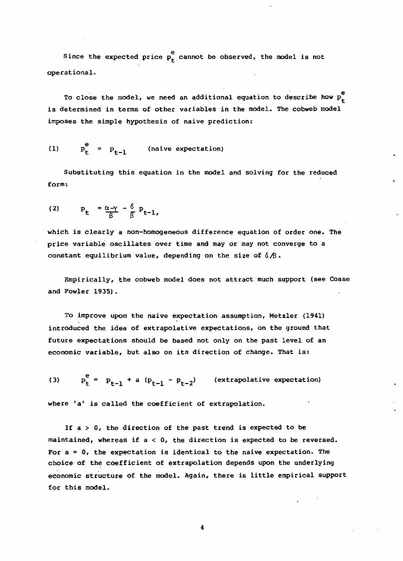
To close the model, we need an additional equation to describe how p~
is determined in terms of other variables in the model. The cobweb model
imposes the simple hypothesis of naive prediction:
(1) = (naive expectation)
Substituting this equation in the model and solving for the reduced
form:
( 2) Pt = CLi,x - 0 p8" t-l,
which is clearly a non-homogeneous difference equation of order one. The
price variable oscillates over time and mayor may not converge to a
constant equilibrium value, depending on the size of 0113.
Empirically, the cobweb model does not attract much support (see Coase
and Fowler 1935).
TO improve upon the naive expectation assumption, Metzler (1941)
introduced the idea of extrapolative expectations, on the ground that
future expectations should be based not only on the past level of an
economic variable, but also on its direction of change. That is:
( 3)e
p =t
(extrapolative expectation)
where 'a' is called the coefficient of extrapolation.
If a > 0, the direction of the past trend is expected to be
maintained, whereas if a < 0, the direction is expected to be reversed.
For a = 0, the expectation is identical to the naive expectation. The
choice-of the coefficient of extrapolation depends upon the underlying
economic structure of the model. Again, there is little empirical support
for this model.
4
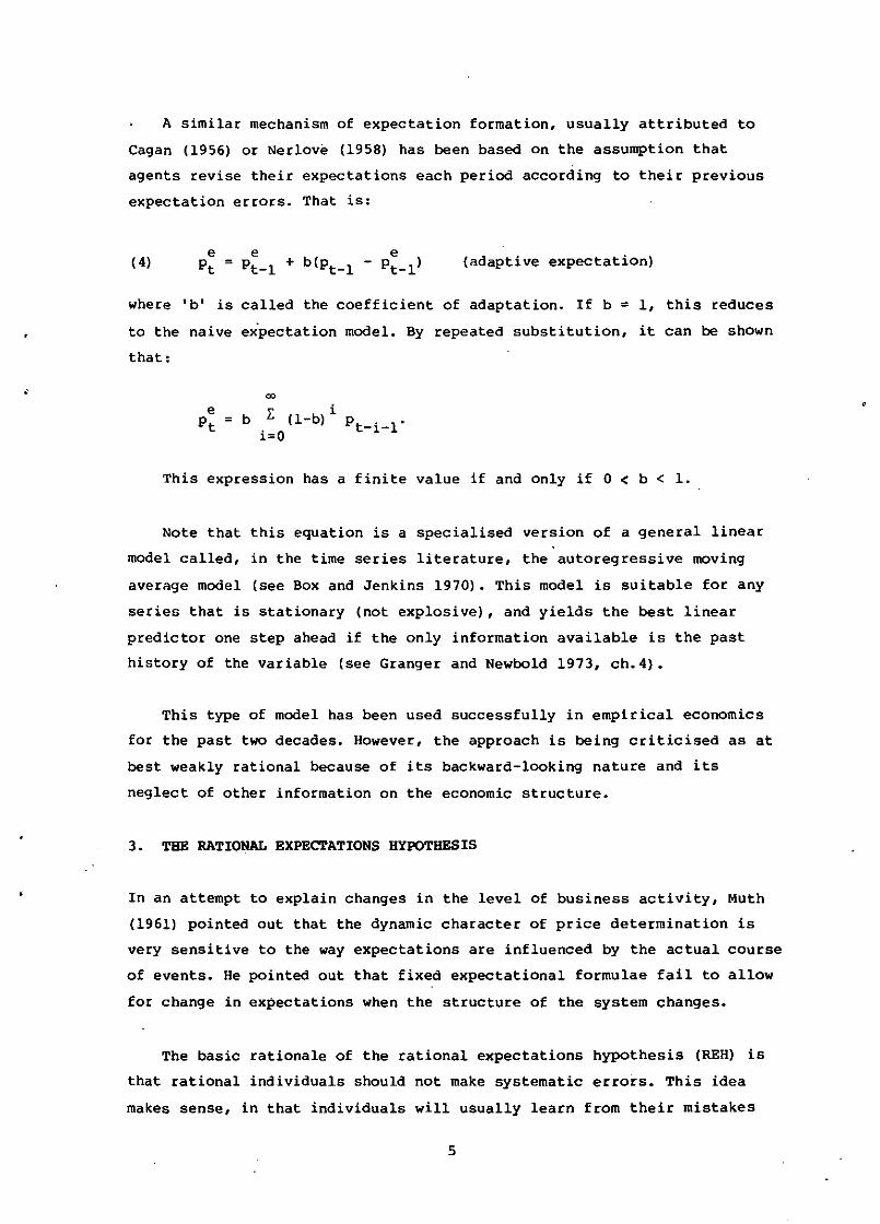
A similar mechanism of expectation formation, usually attributed to
Cagan (1956) or Nerlove (1958) has been based on the assumption that
agents revise their expectations each period according to their previous
expectation errors. That is:
( 4) (adapt I ve expectation)
where 'b' is called the coefficient of adaptation. If b = 1, this reduces
to the naive expectation model. By repeated substitution, it can be shown
that:
<X>
= b E (l_b)i P .. t-,-11=0
This expression has a finite value if and only if 0 < b < 1.
Note that this equation is a specialised version of a general linear
model called, in the time series literature, the autoregressive moving
average model (see Box and Jenkins 1970). This model is suitable for any
series that is stationary (not explosive), and yields the best linear
predictor one step ahead if the only information available is the past
history of the variable (see Granger and Newbold 1973, ch.4).
This type of model has been used successfully in empirical economics
for the past two decades. However, the approach is being criticised as at
best weakly rational because of its backward-looking nature and its
neglect of other information on the economic structure.
3. THE RATIONAL EXPECTATIONS HYPOTHESIS
In an attempt to explain changes in the level of business activity, Muth
(1961) pointed out that the dynamic character of price determination is
very sensitive to the way expectations are influenced by the actual course
of events. He pointed out that fixed expectational formulae fail to allow
for change in expectations when the structure of the system changes.
The basic rationale of the rational expectations hypothesis (REH) is
that rational individuals should not make systematic errors. This idea
makes sense, in that individuals will usually learn from their mistakes
5
and eventually discover the true structure of the underlying system. Thus,
the errors should simply be random movements due to uncertainty and should
tend to cancel each other on average.
In the absence of uncertainty, the REH reduces to the special case of
perfect foresight, because the equilibrium solution of the system is then
uniquely determined. The problem then is w:,ether individuals know the true
structure of the system. Muth did not address this problem; he conjectured
that 'expectations of firms tend to be distributed, for the same
information set, systematically about the prediction of the theory'. If
the theory is wrong and the prediction proves to be inaccurate, then an
REH model cannot be reduced to perfect foresight, even without
uncertainty, unless the rational individuals respecify the model until its
systematic errors are removed. However, for the purpose of empirical
analysis we assume that the prediction of the theory represented in the
form of an econometric model is the true value. In other words, we accept
as the maintained hypothesis that the model is a true description of the
system; rational expectations are then the mathematical expectations
implied by the model conditional on the information available at the time
when expectations must be formed.
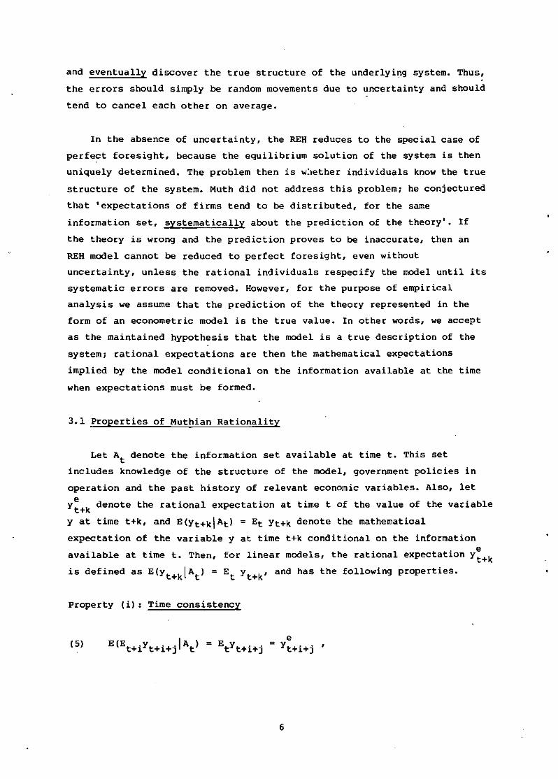
3.1 Properties of Muthian Rationality
Let At denote the information set available at time t. This set
includes knowledge of the structure of the model, government policies in
operation and the past history of relevant economic variables. Also, let
y~+k denote the rational expectation at time t of the value of the variable
y at time t+k, and E(Yt+k!At) = Et Yt+k denote the mathematical
expectation of the variable y at time t+k conditional on the information
available at time t. Then, for linear models, the rational expectation y~+k
is defined as E(Yt+kIAt) = Et Yt+k' and has the following properties.
Property (i): Time consistency
6
that is, individuals have no basis for predicting how they will change
their expectations about future values of a variable.
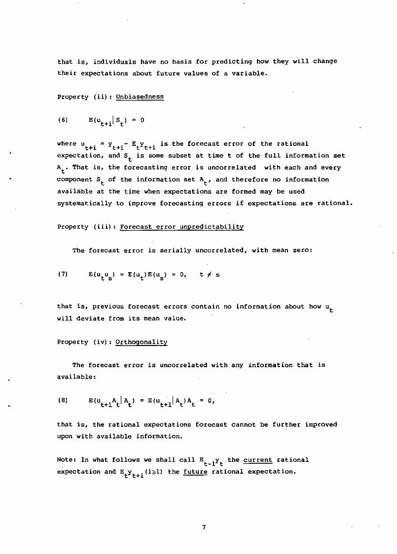
Property (ii): Unbiasedness
where u . =t+1
expectation,
At. That is,
component St
available at
y .- EtYt . is the forecast error of the rationalt+1 +1and St is some subset at time t of the full information set
the forecasting error is uncorrelated with each and every
of the information set At' and therefore no information
the time when expectations are formed may be used
systematically to improve forecasting errors if expectations are rational.
Property (iii): Forecast error unpredictability
The forecast error is serially uncorrelated, with mean zero:
( 7)t '" s
that is, previous forecast errors contain no information about how utwill deviate from its mean value.
Property (iv): Orthogonality
The forecast error is uncorrelated with any information that is
available:
.. ( 8)
that is, the rational expectations forecast cannot be further improved
upon with available information.
Note: In what follows we shall call E lY the current rational. t- t
expectation and E y .(i~l) the future rational expectation.t t+1
7
3.2 Applications of Rational Expectations in Economics
Microeconomic theory is concerned with the existence and optimality of
competitive equilibrium. The Arrow-Debreu model of markets with
uncertainty (Debreu 1959) assumes that 'markets are complete', which is
basically equivalent to assuming certainty. Such a model has been found to
be unrealistic. Radner (1982) analyses the introduction of information and
expectations in models of sequences in incomplete markets. Under the REH,
traders enter the market with different non-price information but use the
market prices to make revisions of their individual models. In
equilibrium, not only are prices determined so as to equate supply and
demand, but individual economic agents correctly perceive the true
relationship between the non-price information received by the market
participants and the resulting equilibrium market prices. A market in
which such a RE equilibrium exists is termed 'informationally efficient'.
Assuming that there is only a finite number of states of initial
information, the concept of REH requires that each trader know the
relationship between initial information and equilibrium prices.
Futia (1979) considered a special case in which there is a market for
a single commodity, the excess supply equations are linear and the
underlying information signals are stationary Gaussian processes. He
established that there exists a symmetric RE equilibrium if and only if
each trader makes as good a conditional prediction of the next period's
price as if he has the pooled information of all traders. This model leads
to an equilibrium theory of stochastic business cycles.
Work on public prediction equilibrium and the 'efficient market
hypothesis' has been done by Jordan (1980) and by Border and Jordan
(1979). Muth's (1961) classic paper used the REH to demonstrate that the
cobweb theorem of price fluctuation is consistent with longer mean cycle
lengths than those implied by extrapolative and non-RE hypotheses.
The popularity of the REH among macroeconomists is primarily due to
the seeming failures of Keynesian macroeconomics in the 1970s, when
stagnation and persistent inflation created a receptive environment for
new ideas.
8
Shiller (1978) and Kantor (1979) have reviewed applications of REH
where the concept is justified as equivalent to profit maximising
expectations for individual agents. If information were free, only the
limits of the Heisenberg uncertainty principle could prevent the REH from
being equivalent to the assumption of perfe~t foresight. Though
information can be acquired only at som~ cost, arbitrage may nevertheless
lead to behaviour corresponding to Muthian rationality.
Sargent and Wallace (1976) used REH and the aggregate supply equation
of Lucas (1972) to provide theoretical support for the controversial
Phelp-Friedman 'invariance' proposition of a vertical Phillips curve
that is, that neither monetary nor fiscal policy has any effect on
unemployment. They also explained why a large proportion of macroeconomic
models typically fail tests for structural change if they ignore rational
expectations.
Lucas's (1976) criticism of the use of conventional econometric
modelling for policy evaluation goes right to the heart of existing
econometric practice. As decision rules are likely to change when the
economic environment changes, simulations using existing models can
provide no useful information as to the actual consequences of alternative
economic policies. REH explicitly exposes this difficulty. However, to
handle models incorporating the concept of REH, the conventional
econometric techniques of identification, estimation, hypothesis testing
and policy simulation are nO longer adequate. The following sections will
deal with each of these problems in turn.
4. STATISTICAL IDENTIFICATION
The 'identification problem' in econometric theory is that of inferring
the structure of a system from information about a reduced-form model. The
classic example of an identification problem arises in demand and supply
analysis. From price and quantity data alone, it is impossible to
determine either the supply or demand curve. Additional information about
the system is needed to estimate the separate demand and supply relations.
In the aggregate supply literature, the problem takes the form of
inability to discriminate between models for which the invariance
9
proposition holds and those in which it does not. Buiter (1980) shows that
an extreme version of the 'Keynesian' model would produce the same reduced
form as a model in which both anticipated and unanticipated money growth
affect output.
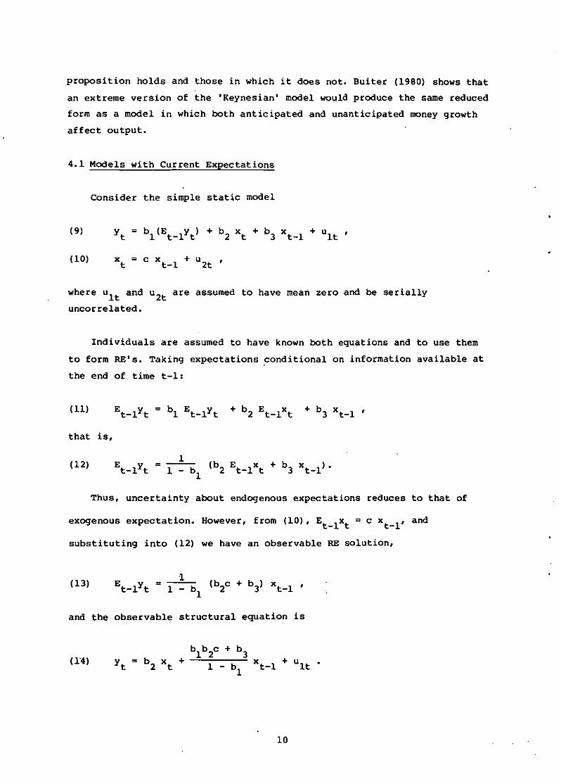
4.1 Models with Current Expectations
Consider the simple static model
where ul t and u2t are assumed to have mean zero and be serially
uncorrelated.
Individuals are assumed to have known both equations and to use them
to form RE's. Taking expectations conditional on information available at
the end of time t-l:
( 11) Et-lYt = bl Et_lyt + b2 Et_lXt+ b
3x
t_l,
that is,
(12) Et-lYt1
(b2 Et_lXt + b3 xt_l)·= 1 - b1
Thus, uncertainty about endogenous expectations reduces to that of
exogenous expectation. However, from (10), Et_lXt = c xt_l' and
substituting into (12) we have an observable RE solution,
(13)
and the observable structural equation is
(H)
10
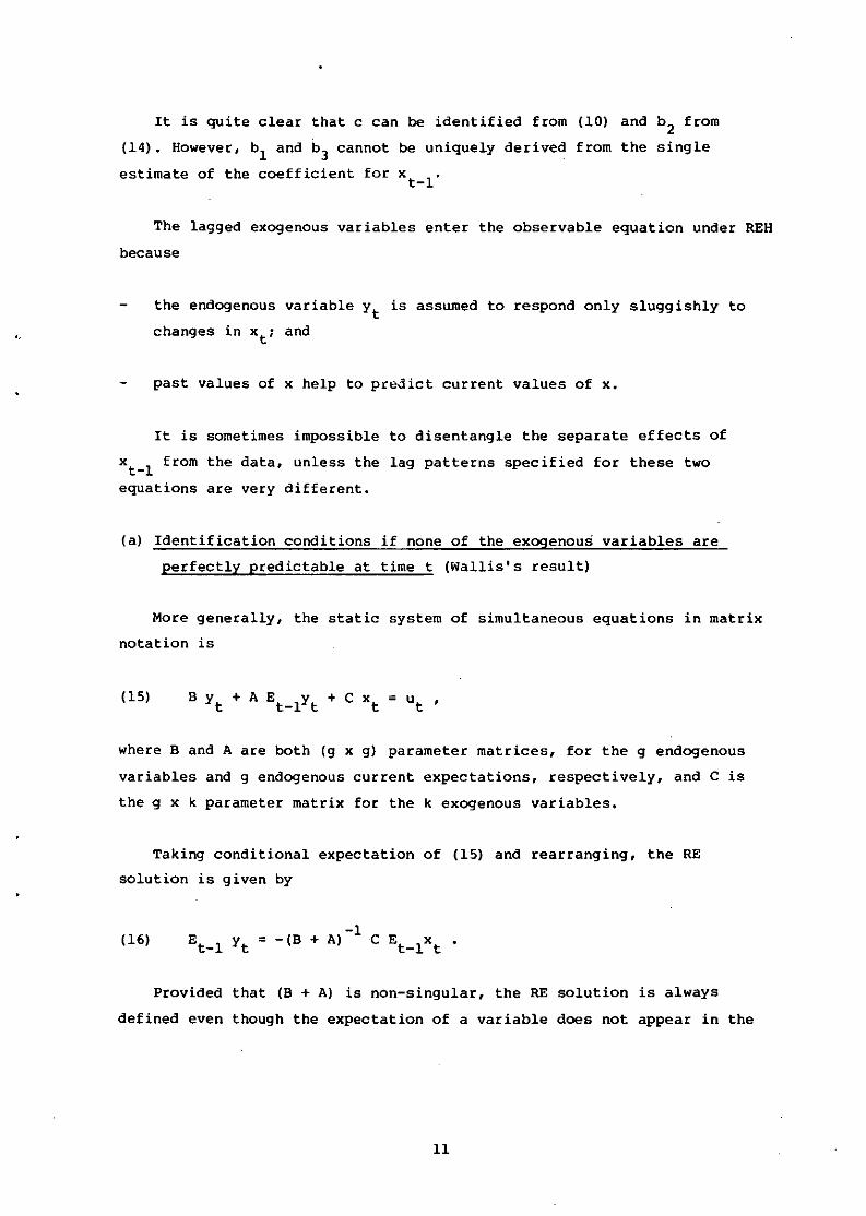
It is quite clear that c can be identified from (10) and
(14). However, bl and b3
cannot
estimate of the coefficient for
be uniquely derived from the
xt-l
b2
from
single
<,
The lagged exogenous variables enter the observable equation under REH
because
the endogenous variable Yt is assumed to respond only sluggishly to
changes in xt; and
past values of x help to predict current values of x.
It is sometimes impossible to disentangle the separate effects of
x 1 from the data, unless the lag patterns specified for these twot-equations are very different.
(a) Identification conditions if none of the exogenous variables are
perfectly predictable at time t (Wallis's result)
More generally, the static system of simultaneous equations in matrix
notation is
where B and A are both (g x g) parameter matrices, for the g endogenous
variables and g endogenous current expectations, respectively, and C is
the g x k parameter matrix for the k exogenous variables.
Taking conditional expectation of (15) and rearranging, the RE
solution is given by
(16)-1= -(B + A)C Et_lX
t
Provided that (B + A) is non-singular, the RE solution is always
defined even though the expectation of a variable does not appear in the
11
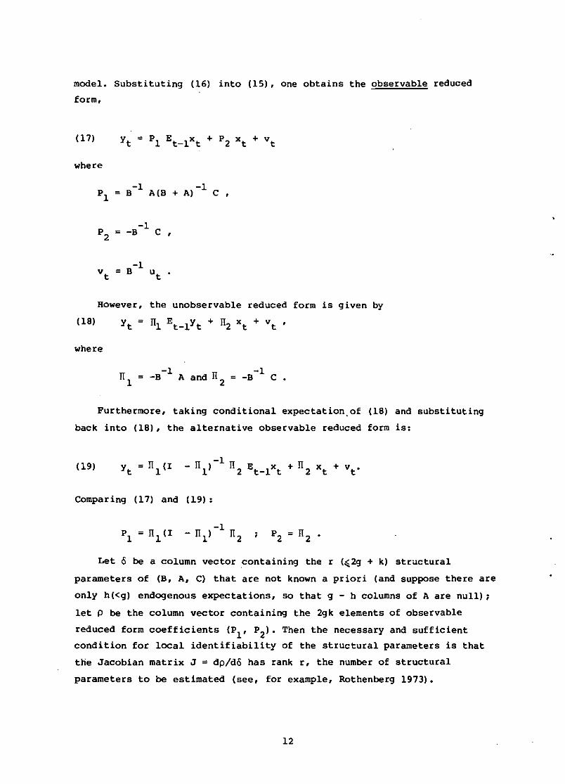
model. Substituting (16) into (15), one obtains the observable reduced
form,
where
-1 -1= B A(B + A) C,
-1= -B C,
-1v = B ut t .
However, the unobservable reduced form is given by
(18) Yt = III Et-lYt + I12 xt + vt '
where
-1 -1III = -B A and II2 = -B C.
Furthermore, taking conditional expectation,of (18) and substituting
back into (18), the alternative observable reduced form is:
Comparing (17) and (19):
Let 0 be a column vector .containing the r (~2g + k) structural
parameters of (B, A, C) that are not known a priori (and suppose there are
only h«g) endogenous expectations, so that g - h columns of A are nUll) 1
let P be the column vector containing the 2gk elements of observable
reduced form coefficients (PI' P2). Then the necessary and sufficient
condition for local identifiability of the structural parameters is that
the Jacobian matrix J = dp/do has rank r, the number of structural
parameters to be estimated (see, for example, Rothenberg 1973).
12
o·
"
e
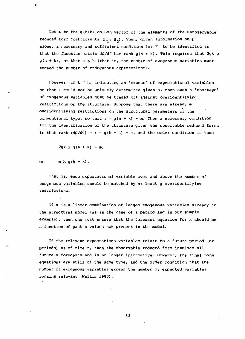
Let TI be the g(h+k) column vector of the elements of the unobservable
reduced form coefficients (TIl' TI2).
Then, given information on p
alone, a necessary and sufficient condition for TI to be identified is
that the Jacobian matrix dP/dTI has rank g(h + k). This requires that 2gk ~
g(h + k), or that k ~ h (that is, the number of exogenous variables must
exceed the number of endogenous expectations).
However, if k < h, indicating an 'excess' of expectational variables
so that TI could not be uniquely determined given P, then such·a 'shortage'
of exogenous variables must be traded off against over identifying
restrictions On the structure. Suppose that there are already m
over identifying restrictions on the structural parameters of the
conventional type, so that r = g(h + k) - m. Then a necessary condition
for the identification of the structure given the observable reduced forms
is that rank (dP/do) = r = g(h + k) - m, and the order condition is then
2gk " 9 (h + k) - m,
or m ~ g(h - k).
That is, each expectational variable over and above the number of
exogenous variables should be matched by at least 9 overidentifying
restrictions.
If x is a linear combination of lagged exogenous variables already in
the structural model (as is the case of 1 period lag in our simple
example), then one must ensure that the forecast equation for x should be
a function of past x values not present in the model.
If the relevant expectations variables relate to a future period (or
periods) as of time t, then the observable reduced form involves all
future x forecasts and is no longer informative. However, the final form
equations are still of the same type, and the order condition that the
number of exogenous variables exceed the number of expected variables
remains relevant (Wallis 1980).
13
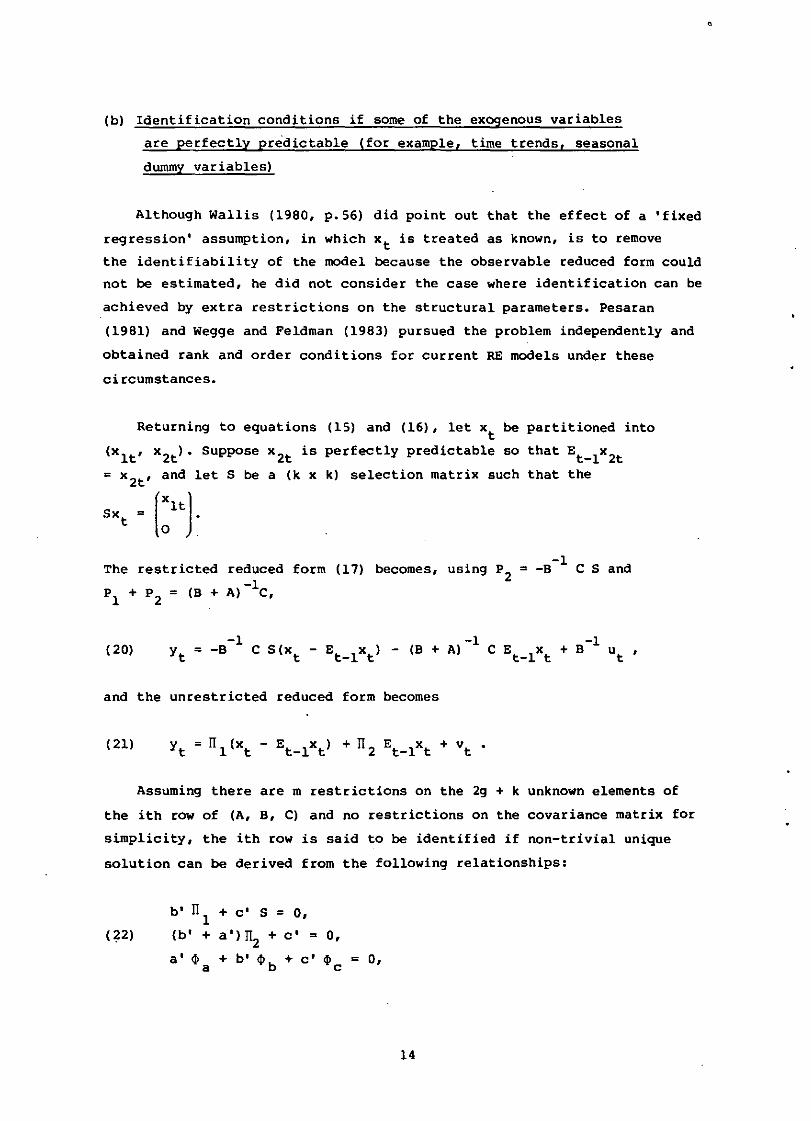
(b) Identification conditions if some of the exogenous variables
are perfectly predictable (for example, time trends, seasonal
dummy variables)
Although Wallis (1980, p.S6) did point out that the effect of a 'fixed
regression' assumption, in which x t is treated as known, is to remove
the identifiability of the model because the observable reduced form could
not be estimated, he did not consider the case where identification can be
achieved by extra restrictions on the structural parameters. Pesaran
(1981) and Wegge and Feldman (1983) pursued the problem independently and
obtained rank and order conditions for current RE models under these
circumstances.
k) selection matrix such that
Returning to equations
(x l t' x 2t)· Suppose x 2t is
= x 2t' and let S be a (k x
sXt = [:It(15) and (16), let x
tbe
perfectly predictable so
partitioned into
that
The restricted reduced
PI + P2
= (B + A)-lC,
-1form (17) becomes, using P2 = -B C Sand
( 20)
and the unrestricted reduced form becomes
Assuming there are m restrictions on the 2g + k unknown elements of
the ith row of (A, B, C) and no restrictions on the covariance matrix for
simplicity, the ith row is said to be identified if non-trivial unique
solution can be derived from the following relationships:
b' Jl + c' S = 0,1(?2) (b' + a') ~ + c· = 0,
a' 4> + b' 4> + c" 4> = 0,a b c
14
"
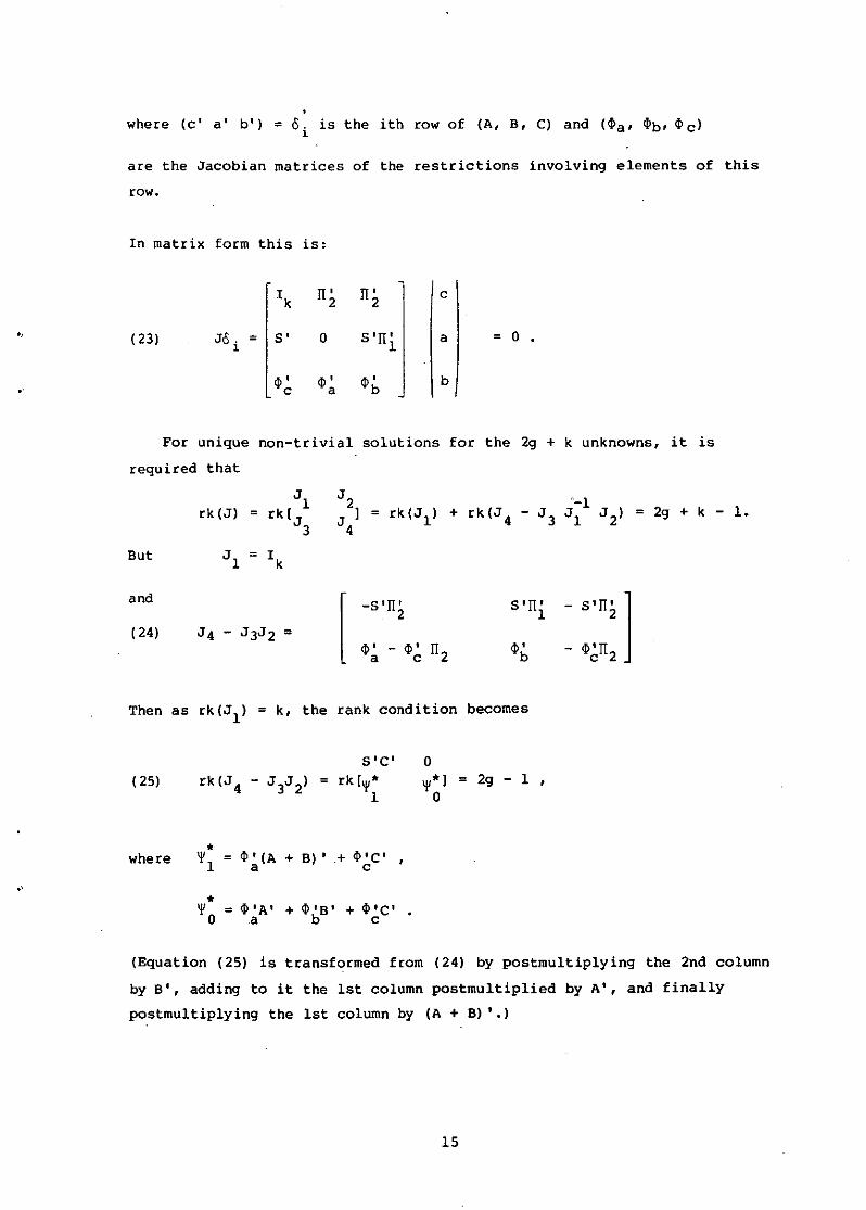
,where (c' a' b'l = '\ is the ith row of (A, B, C) and (<I>a' <l>b' <l>cl
are the Jacobian matrices of the restrictions involving elements of this
row.
In matrix form this is:
I k II' II' c2 2
( 23) J8 i = S' a S 'n ' a = a .1
<I> ' <1>' <1>' bc a b
For unique non-trivial solutions for the 2g + k unknowns, it is
required that
Jl
J 2 + rk(J 4 - J 3'-1
2g+k-1.rk (Jl = rkl J J ] = rk(Jl) Jl
J 2) =3 4
But J l = Ik
and
[_sIn' S'I1' - ,orr; ]2 1
(24) J4 - J3J2 =<1>' - <1>' I1 2
<1>' <I>'I1a c b c 2
Then as rk(Jl) = k, the rank condition becomes
( 25)S'C'
= rk ['1'*1
a'1'*] = 2g - 1 ,
a
where*
'1'1 = <1>' (A + B) , .+ <I>'C'a c
*'1'0 = ~'A' + ¢ IB' + <I>'c'
a b c
(Equation (25) is transformed from (24) by postmultiplying the 2nd column
by B', adding to it the 1st column postmultiplied by A', and finally
postmultiplying the 1st column by (A + B) '.)
15
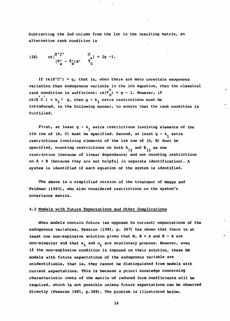
Subtracting the 2nd column from the 1st in,the resulting matrix, an
alternative rank condition is
( 26)
If rk(S'C') = g, that is, when there are more uncertain exogenous
variables than endogenous variable in the ith equation, then the classical•rank condition is sufficient: rk(~O) = g - 1. HOwever, if, ,
rk (S C ) = kl < g, then g - kl extra restrictions must be
introduced, in the following manner, to ensure that the rank condition is
fulfilled.
First, at least g - kl extra restrictions involving elements of the
ith row of (A, C) must be specified. Second, at least g - kl
extra
restrictions involving elements of the ith row of (A, B) must be
specified, counting restrictions on both A.. and B.. as one1) 1)
restriction (because of linear dependence) and not counting restrictions
on A + B (because they are not helpful in separate identification). A
system is identified if each equation of the system is identified.
The above is a simplified version of the treatment of Wegge and
Feldman (1983), who also considered restrictions on the system's
covariance matrix.
4.2 Models with Future Expectations and Other Complications
When models contain future (as opposed to current) expectations of the
endogenous variables, Pesaran (1981, p. 387) has shown that there is at
least one non-explosive solution given that B, B + A and B - A are
non-singular and that xt and ut are stationary process. However, even
if the non-explosive condition is imposed on their solution, these RE
models with future expectations of the endogenous variable are
unidentifiable, that is, they cannot be distinguished from models with
current expectations. This is because a priori knowledge concerning
characteristic roots of the matrix of reduced form coefficients will be
required, which is not possible unless future expectations can be observed
directly (Pesaran 1981, p.389). The problem is illustrated below.
16
"
.'
(a) Single equation models with future expectation
Identification of models with future RE starts from finding their
reduced forms. For the most part, these models are systems of linear
stochastic difference equations in which agents' views about the future
enter in a specific way. If these expectations are formed adaptively, the
problem of finding a reduced form is equivalent to finding the solution to
a standard difference equation. But when expectations are assumed to be
rational, the search for a reduced form is transformed into a rather more
complicated search for a fixed point. Suppose that expectations of future
variables can be written as linear functions of available information. One
can calculate the reduced form using standard techniques, and the reduced
form can be used to forecast the same variables that agents were
interested in. The model is solved when the forecasts of agents match
those of the reduced form.
Since RE models are 'expectational difference equations', special
techniques are needed to find the reduced-form solution with the fixed
point property of REH. There is a wide range of techniques suggested in
the literature to deal with the problem. One can find •state-space'
technique in Lucas (1972), 'operator' methods in Sargent (1979) and Wallis
(1980), 'methods of undetermined coefficients' in time domain in Muth
(1961) and Aoki and Canzoneri (1979), and 'forward' and 'backward'
solutions in Blanchard (1979). However, these techniques are basically of
two kinds: one transforms an expectational difference equation into
another ordinary difference equation; the other transforms the
expectationa1 difference equation into a system of non-linear algebraic
equations. All of them tend to go too far toward obtaining closed form
solutions and are often intractable or conceal the existence and
uniqueness problems •
Whiteman (1983) proposes a simplified version of the method of
'undetermined coefficients in the frequency domain' which was due to
Saracoglu and Sargent (1978) and Futia (1981). In comparison with the
standard techniques, this technique is simpler computationally due to the
availability of existing algorithms for power spectrum estimation. The
technique could be used in conjunction with a maximum likelihood procedure
for estimating the parameters of the expectational difference equation
under the cross-equation restrictions of RE.
17
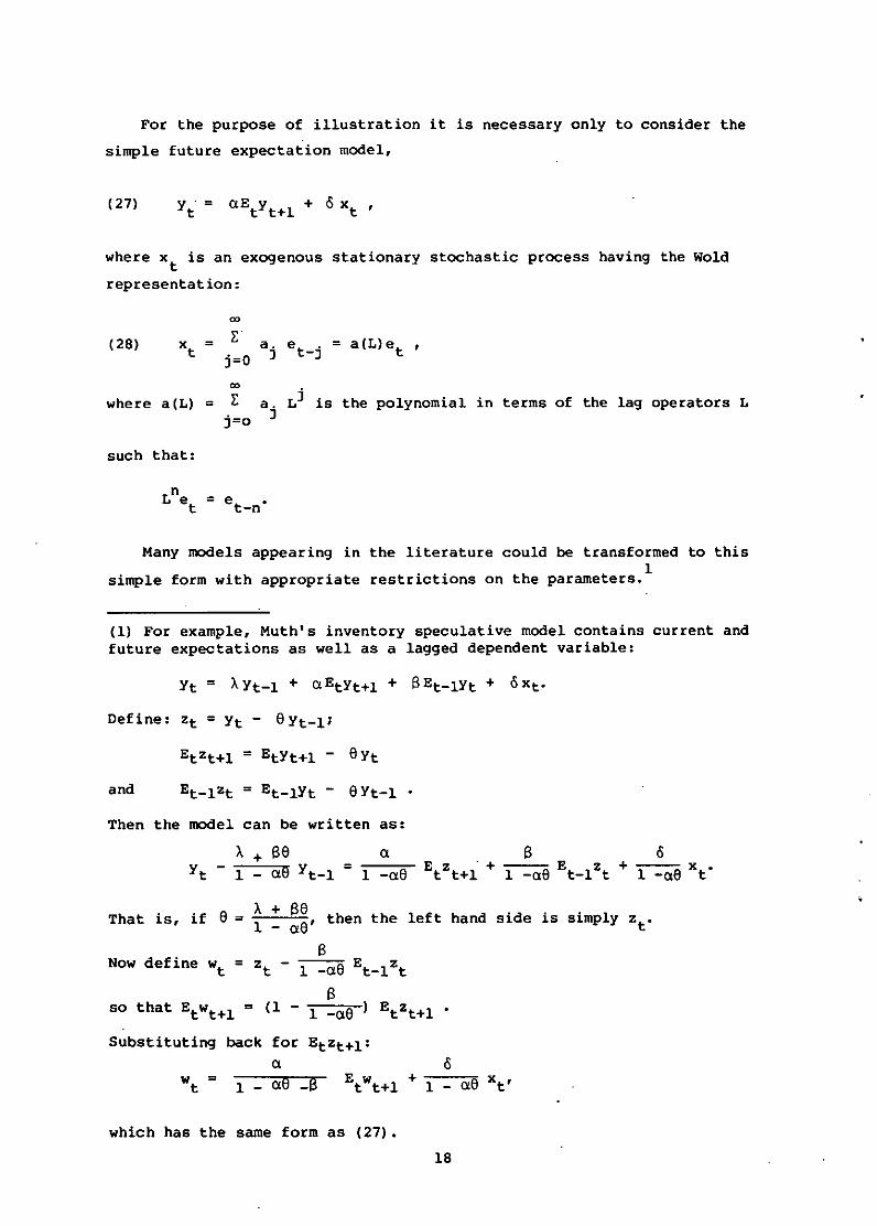
For the purpose of illustration it is necessary only to consider the
simple future expectation model,
where xt
is an exogenous stationary stochastic process having the Wold
representation:
00
xt
= 1: a. e t .j=O J -J
where a (L)
such that:
00
= 1: a.j=o J
Lj is the polynomial in terms of the lag operators L
nL e
t= e t 0
-n
Many models appearing in the literature could be transformed to this1
simple form with appropriate restrictions on the parameters.
(1) For example, Muth's inventory speculative model contains current andfuture expectations as well as a lagged dependent variable:
Define: Zt = Yt - S Yt-l1
Then the model can be written as:
a-as
o1 -as
That is, if S A + 8S= 1 _ as' then the left hand side is simply Zt O
8Now define wt = Zt - 1 -as Et_lZt
8so that Etwt+l = (1 - 1 -as ) EtZt+l
Substituting back for EtZt+l:a
wt = 1 - as -5
which has the same form as (27)0
18
"
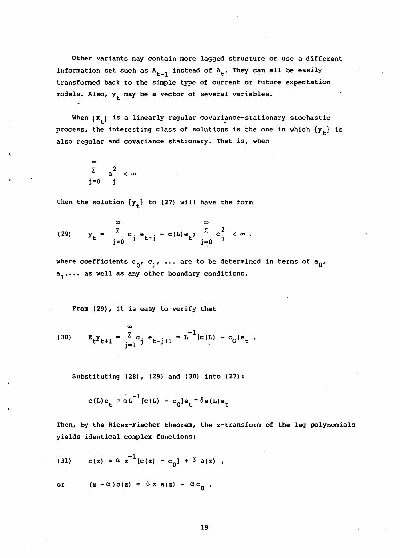
Other variants may contain more lagged structure or use a different
information set such as At_l instead of At' They can all be easily
transformed back to the simple type of current or future expectation
models. Also, Yt may be a vector of several variables.
When {Xt} is a linearly regular covariance-stationary stochastic
process, the interesting class of solutions is the one in which {Yt} is
also regular and covariance stationary. That is, when
'" 2a < co
j=O j
then the solution {Yt} to (27) will have the form
( 29)
cc
I:
j=Oc. e
t.
J -J
co
I:
j=O
2c.
J<00.
where coefficients cO' c l' ••• are to be determined in terms of aD,
a l, ••• as well as any other boundary conditions.
From (29), it is easy to verify that
00
(30) I: c.j=l J
.'
SUbstituting (28), (29) and (30) into (27):
Then, by the Riesz-Fischer theorem, the z-transform of the lag polynomials
yields identical complex functions:
( 31) c (z)-1=Q z [c(z) - cOl + 6 a(z) ,
or (z -Q )c(z) = 6 z a(z) - QC O •
19
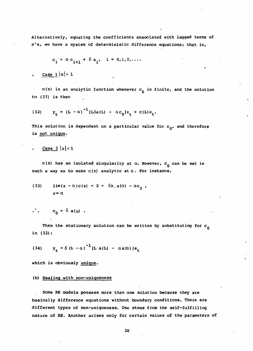
Alternatively, equating the coefficients associated with lagged terms of
e's, we have a system of deterministic difference equationsl that is,
case llal> 1
c(z) is an analytic function whenever Co is finite, and the solution
to (27) is then
( 32)
This solution is dependent on a particular value for cO' and therefore
is not unique.
Case 2 lal < 1
c(z) has an isolated singularity at a. However, Co can be set in
such a way as to make c(z) analytic at a. For instance,
(33) lim(z - a )c(z) = 0 = ca. ala) - ac O '
z-a
c = c ala) •o
Then the stationary solution can be written by sUbstituting for Coin (32):
( 34)-1
Yt = C (L - a ) [L a (L) - a a (a) )e t
which is obviously unique.
(b) Dealing with non-uniqueness
Some RE models possess more than one solution because they are
basically difference equations without boundary conditions. There are
different types of non-uniqueness. One stems from the self-fulfilling
nature of RE. Another arises only for certain values of the parameters of
20
the model. Taylor (1977) claimed that a widely publicised leading
indicator of a future variable may be taken as genuine even if in fact it
consists simply of random numbers. This 'leading indicator' problem arises
in a model-of future expectations if the information set is-At_l•
If the
information set is At then a spurious 'coincident' indicator rather than
'leading' indicator would be admitted as the source of non-uniqueness.
Thus a spurious indicator is-actually just one solution to the homogeneous
equation. When initial values are specified for the sequence Yt the
indeterminacies disappear. When such boundary conditions are not present,
some other side condition is necessary to eliminate these indeterminacies.
Two methods for dealing with non-unique solutions have been suggested.
One method is to choose the one with the smallest variance (Taylor 1977)
and the other is to choose the smallest set of variable from which a
solution can be calculated (McCallum 1983). However, these methods have
their limitations. It can be shown (see Whiteman 1983) that Taylor's
method may produce a Yt which fails to have an autoregressive
representation. Also the method may not be compatible with the unique
solution imposed by the parameters of the model. On the other hand,
McCallum's method may prove intractable, because it is possible to obtain
a solution but not recognise that it is only one of many solutions, and
the computational burden of solving non-linear equations increases as the
order of the difference equation increases.
To avoid the above mentioned problems, the following additional
strategies might be adopted. The first is to require that the sOlution
hold for a given value of Yt-l' say at t - to' This amounts to using
an initial condition to determine a solution. The second is to require
that the solutions be functions of the objective features of the
environment. However, the existence and uniqueness of such solutions are
completely determined by the parameters of the model. For a particular set
of parameters, a model may have one solution, many solutions, or no
solution. It may be argued that multiple equilibria are admissible
solutions under RE - that all of them will have a second desirable
property and it is up to the researcher to specify this within the set of
admissible solutions. Finally, Chow (1983, p.361) has proposed that the
uniqueness issue be resolved empirically: that is, that the extra
21
parameter be estimated from the data. This procedure serves to highlight
the non-uniqueness of RE solutions rather than concealing the problem.
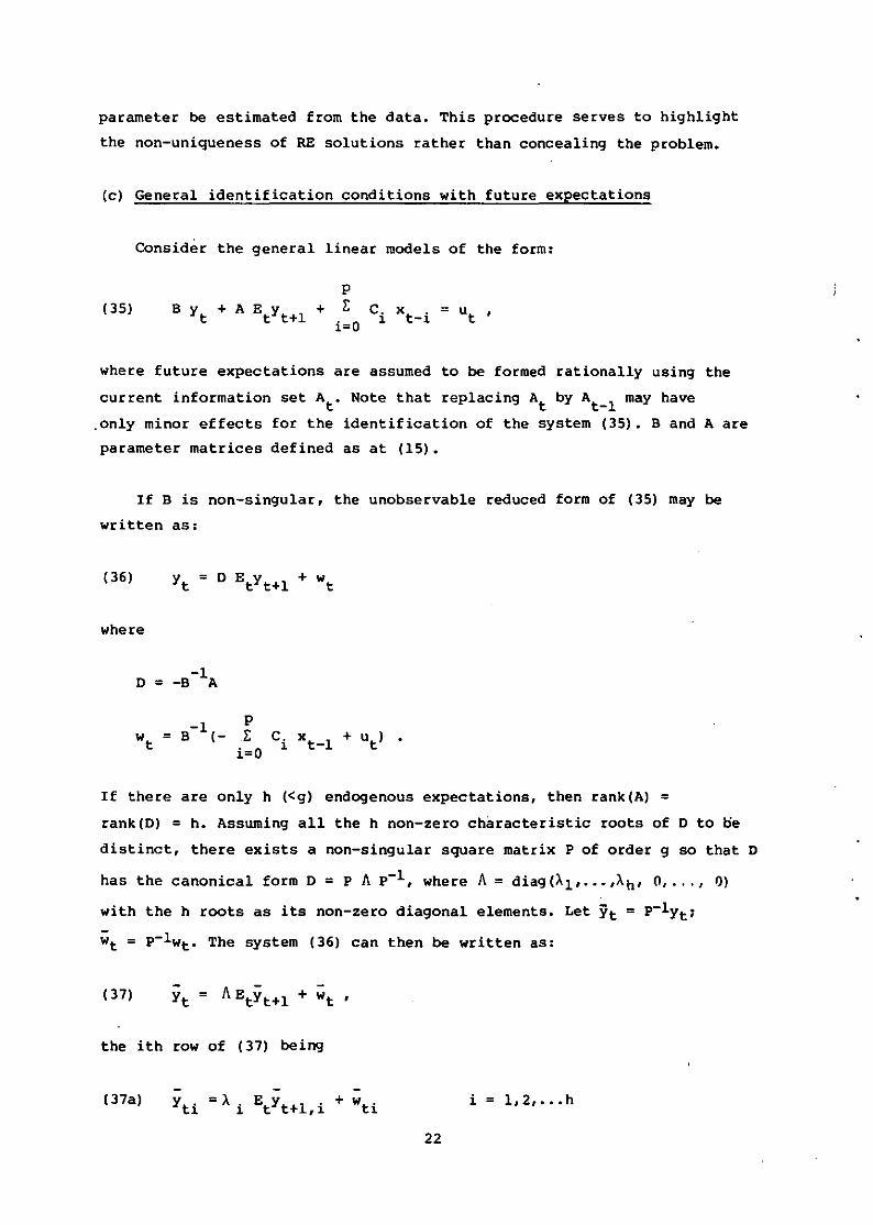
(c) General identification conditions with future expectations
Consider the general linear models of the form:
(35) B Y + A E Y +t t t+l
pE
i=O
where future expectations are assumed to be formed rationally using the
current information set At. Note that replacing At by At_lmay have
.only minor effects for the identification of the system (35). B and A are
parameter matrices defined as at (15).
If B is non-singular. the unobservable reduced form of (35) may be
written as:
where
D = _B-1A
If there are only h «g) endogenous expectations, then rank(A) =rank(D) = h. Assuming all the h non-zero characteristic roots of D to be
distinct. there exists a non-singular square matrix P of order g so that D
has the canonical form D = P A p-l. where A = diag(Al •••••Ah. 0, ... r I)
with the h roots as its non-zero diagonal elements. Let Yt = p-1Yt1
wt = p-1Wt. The system (36) can then be written as:
the ith row of (37) being
(37a) Y =A.Ey +wti 1 t t+l.i ti
22
i = 1,2, ... h
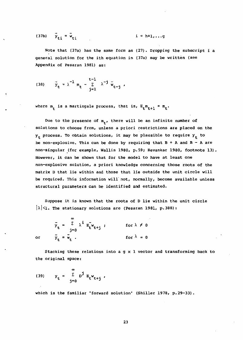
(37b) i ::: h+ 1, ••. 9
Note that (37a) has the same form as (27). Dropping the subscript i a
general solution for the ith equation in (37a) may be written (see
Appendix of Pesaran 1981) as:
(38) m t
t-lE
j=l
where mt is a martingale process, that is, Etmt +l = mt•
Due to the presence of mt, there will be an infinite number of
solutions to choose from, unless a priori restrictions are placed on the
Yt process. To obtain solutions, it may be plausible to require Yt to
be non-explosive. This can be done by requiring that B + A and B·- A are
non-singular ,(for example, Wallis 1980, p.59; Revankar 1980, footnote 13).
However, it can be shown that for the model to have at least one
non-explosive solution, a priori knowledge concerning those roots of the
matrix D that lie within and those that lie outside the unit circle will
be required. This information will· not, normally, become available unless
structural parameters can be identified and estimated.
Suppose it is known that the roots of D lie within the unit circle
jA!<l. The stationary solutions are (Pesaran 1981, p.388):
ro
E Ai -Yt = EtWt +jj=O
or Yt = wt .
Stacking these relations
the original space:
ro
(39) Yt = E Dj
EtWt +jj=O
for A to 0
for A = 0
into a g x 1 vector and transforming back to
which is the familiar 'forward solution' (Shiller 1978,.p.29-33).
23
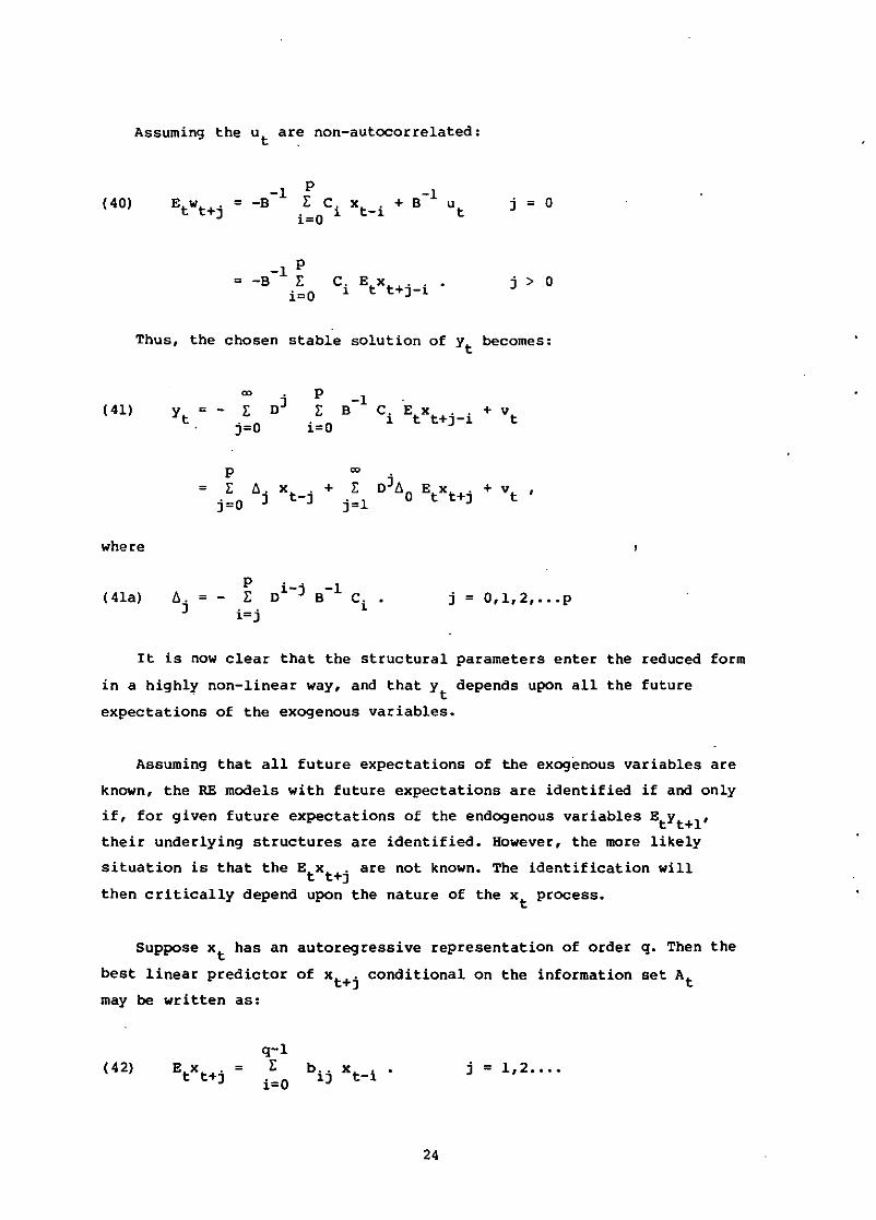
Assuming the ut are non-autocorrelated:
( 40)-1= -B
PL c.
i=O 1j = 0
-1 P= -B L
i=Oj > 0
( 41)
Thus. the chosen stable solution of Yt becomes:
00
Dj P -1
Yt = - L L B C. EtXt +j_i + vtj=O i=O 1
P 00
= L /:'. Xt . + L Dj/:,EtXt +j + vt •
j=O J -J j=l 0
where
( 41a) j = 0.1.2•••• p
It is now clear that the structural parameters enter the reduced form
in a highly non-linear way. and that Yt depends upon all the future
expectations of the exogenous variables.
Assuming that all future expectations of the exogenous variables are
known. the RE models with future expectations are identified if and only
if. for given future expectations of the endogenous variables Etyt +l•their underlying structures are identified. However. the more likely
situation is that the EtXt +j are not known. The identification will
then critically depend upon the nature of the xt
process.
Suppose xt has an autoregressive representation of order q. Then the
best linear predictor of xt +j conditional on the information set At
may be written as:
( 42)q-lL
i=O
24
j = 1.2 ••••
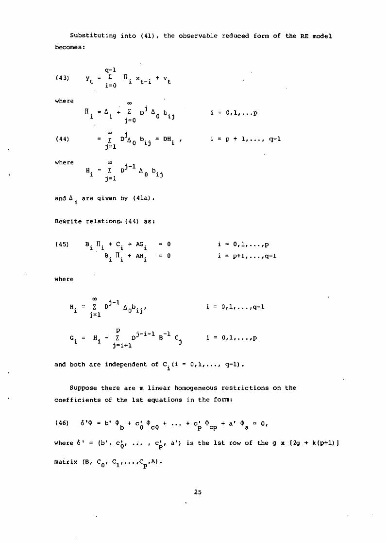
Substituting into (41), the observable reduced form of the RE model
becomes:
q-l(43) Yt
= r IT. xt
_i
+ vti=O 1
where 00
IT = (j + r oj (j b ..i i j=O
0 1)
00
oj(j( 44) = r b .. = OH.j=l 0 1) 1
where 00j-l
H. = E n (j 0 b ..1 j=l 1)
and (j . are given by (41a) •1
Rewrite relations. (44) as:
(45) B. IT. + C. + AG. = 01 1 1 1
B. IT. + AM. = 01 1 1
where
eej-l
H. = z n (jObi j,1 j=l
pj-i-l -1G. = H. - r 0 B C.
1 1 j=i+1 )
i::;;:O,l, ••• p
i = p + 1, •.. , q-l
i=O,l, ,p
i = p+l, ,q-l
i = 0,1, ... ,q-l
i=O,l, ... ,p
and both are independent of C. (i = 0,1, •.• , q-l).1
Suppose there are m linear homogeneous restrictions on the
coefficients of the 1st equations in the form:
( 46) o'<I>=b'<I>b+C'<I> + +c'<I> +a'<I> =0,o cO '" p cp a
where 0' = (b', cO' .~. , cp' a') is the 1st row of the g x [2g + k(p+l»)
25
'r~l ojni pnijujiJadUe
: asmo:)sc'
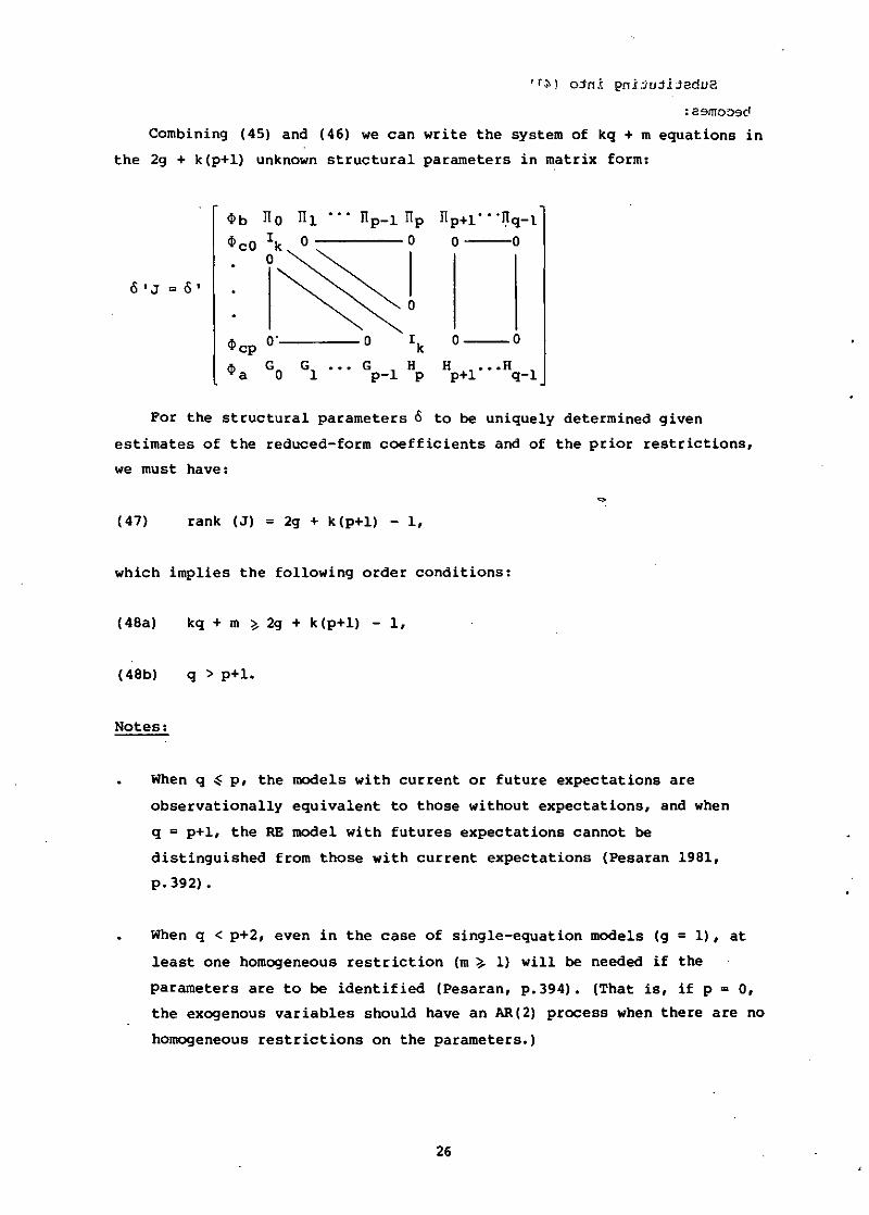
Combining (45) and (46) we can write the system of kq + m equations in
the 2g + k(p+l) unknown structural parameters in matrix form:
<l>b TIO TIl ••• TIp-l TIp
.o':~:
<l>cp 0"---- 0 I k<l>a Go Gl Gp_l Hp
TIpH" • 'TIq-l
o 0
o 0
H ••• HpH q-l
For the structural parameters 6 to be uniquely determined given
estimates of the reduced-form coefficients and of the prior restrictions,
we must have:
(47) rank (J) = 2g + k (pH) - 1,
which implies the following order conditions:
( 48a)
(48b)
Notes:
kq + m ~ 2g + k (pH) - 1,
q > p+l.
When q ~ p, the models with current or future expectations are
observationally equivalent to those without expectations, and when
q = p+l, the RE model with futures expectations cannot be
distinguished from those with current expectations (Pesaran 1981,
p. 392) •
When q < p+2, even in the case of single-equation models (g = 1), at
least one homogeneous restriction (m ~ 1) will be needed if the
parameters are to be identified (Pesaran, p.394). (That is, if p = 0,
the exogenous variables should have an AR(2) process when there are no
homogeneous restrictions on the parameters.)
26
If q ~. p+2 and k (q-p-l) < g, then the necessary condition is that qk
exceeds the number of variables included in that equation less 1
(Pesaran, p.394).
If q~. p+2 and k (q-p-l) ~ g, the necessary condition for
identification could be investigated simply by treating all the
expectation variables as if they were observable and exogenously given
(Pesaran, p.394). This becomes the classical condition for
identification, that there should be at least g - 1 independent linear
restrictions on the parameters of that equation (m ~ g-l).
5. ESTIMATION PROBLEMS
It is well known that, when structural equations are overidentified,
'full information' methods such as 3SLS will be more efficient than
'limited information' methods such as 2SLS. Since many of the RE
restrictions are cross-equation, it might seem natural to use full
information methods. However, estimation by full information methods is
very sensitive to model misspecification and incorrect restrictions. Thus,
many researchers prefer limited information methods so as to hedge against
these problems.
Another issue in the estimation of models with RE is that proxies for
anticipated and unanticipated variables have to be constructed in the form
of predictors or residuals from an estimated equation. For instance,
Anderson et al. (1976) and Duck et al. (1976) used predictors of ARMA
models to replace anticipation variables. Barro (1977) and Sheffrin (1979)
proxied unanticipated quantities with the residuals of the one-period
predictions. To overcome possible inconsistency in the resulting
estimates, Wickens (1982) and Mccallum (1976a) considered the 'errors in
variables' method and Wallis (1980) proposed a three-step method. The
latter two approaches will be examined below in reverse order.
Wallis (1980) considered estimation of model (15) assuming that the
structure is identified.
The three-step method of Wallis comprises
27
~
Step 1: Estimate Et_lxt by x t' from the exogenous process
conditional on the past history of all variables in the system,
~ ~
Step 2: Given that xt = xt + et, the observable reduced'form at
(19) becomes
(49)
~
which can be estimated consistently by OLS to obtain the predictions Yt'
Step 3: Apply 2SLS to the structural equations ,after Et_1Yt in~
(15) has been replaced by Yt'
Pagan (1984, p.230) demonstrated that while the coeffigients estimated
by Wallis are consistent, the estimated covariance matrix is generally
inconsistent. However, if Et-1Yt is to be replaced by the actual~
values, Yt' with Yt included among the set of predetermined variables
in the reduced form, the resulting estimated covariance matrix is
consistent while the parameter estimates are unaffected.
McCallum (1976a) used the actual value Yt as a proxy for the
expectations variable Et-lyt, Such a substitution induces an 'errors
in variables' problem, since Yt is now a stochastic regressor which is
correlated with the augmented disturbance term. Note that the RE
forecasting errors consist of both shocks due to exogenous variables and
reduced-form disturbances, and therefore are contemporaneously correlated
with the exogenous variables. Thus, instrumental variables are required
for both Yt
and xt in order to obtain consistent estimates for the
equation. This approach suffers from perfect multicollinearity if the
structural equation consists of the endogenous variable and its own RE
simultaneously. Furthermore, current exogenous variables can no longer be
used as instruments due to correlation with the error term, and the
identification condition is now more stringent.
One advantage of McCallum's approach is that one can now do without
specifying and estimating the autoregressive model for the exogenous
variables, In fact, consistent estimates are now obtained by a single
application of the method of instrumental variables.
28
For a dynamic model involving future expectation of endogenous
variables, the use of actual values as proxies can. also be applied
(Mccallum 1976b). But this approach must be sUbject to further
identifiability problems in large systems (Wallis 1980 p.68).
With regard to non-linear models, there has been relatively little
research done. Fair and Taylor (1983) have investigated a full information
estimation method for a nonlinear model. However, the solution procedure,
-based on the Gauss-Siedel algorithm, was found to be extremely expensive
to use. Hansen and Singleton (1982) have developed and applied -a limited
information estimator for non-linear models.
6. HYPOTHESIS TESTING
Restricting attention to linear models, the implication of the RE
hypothesis is that the expectation assessed by the market equals the
conditional expectation using all available past information. That is:
which implies that
(50)
The error of market expectation has zero mean and is uncorrelated with any
past information.
A form of the RE model that has been used extensively in empirical
work is:
(51)
This model has been used to study the rationality of interest rate and
inflation forecasts in the bond market and many other applications in the
efficient-market literature (for example, Dornbusch 1976, Frenkel 1981).
It was also used to display the policy ineffectiveness proposition by
Sargent and Wallace (1975), Barro (1979) and Grossman (1979). Lagged terms
29
have also been included in the model, to capture dynamics (see Shiller
1980, Bernanke 1982). The hyPOthesis of rationality implies thate e
Et_l Yt = Yt and Et_l xt = xt' whereas the hypothesis of neutrality (or
policy
lagged
ineffectiveness) implies thateterms of xt are also zero).
o = 0 (and that the coefficients of
To be able to test the hyPOthesis of
linear forecasting model for xt•
Suppose
where
rationality, we need to specify a
that
zt-l
= a column vector of variables used to forecast xt
which are
available at t-l,
Y = a column vector of coefficients,
ut = serially uncorrelated errors.
Taking expectation of equation (52) conditional on information available
at t-l:
,(53) Et_ l xt = Zt_l Y*
and, substituting into equation (51),
( 54)
If the y-equation is a reduced form so that all the right-hand side
variables are exogenous and are uncorrelated with the error term, then OLS
will yield consistent estimates of S. An identification problem exists if
Zt_l includes only lagged values of xt while equation (53) is a
distributed lag of x in the model (see Sargent 1976). This is the case
illustrated in section 4.1 above.
30
If the model is unidentified, then a model with 6 = 0 is
observationally equivalent to that with 6 # o. To avoid this problem, the
researcher must ensure that either (a) there is no distributed lag of x in
the y-equation or (b) the forecasting model for x includes lagged values
of at least one other variable besides x which does not enter the
y-equation as a separate variable. If the equation is identified, then a
test of rationality is equivalent to a test of the equality of the
coefficients Y estimated in (52) and (54). This cross-equation restriction
y =y. can be tested by the likelihood ratio statistic:2
that is, by
comparing the maximum likelihood function of the system (52) and (54)
estimated jointly, with and without imposing the cross-equation
restriction.
The hypotheses both of rationality (Y =Y*) and of neutrality (6 = 0)
can be tested as a joint hypothesis. However, neutrality has meaning only
if we have a theory of expectation such as the RE hypothesis. Thus, the
test of the rationality hypothesis assuming neutrality would not 'yield
useful inform~tion.
Note that the test may be rendered invalid if relevant variables are
omitted from the model and if the 'error terms are serially correlated. On
the other hand, it is known that the addition of irrelevant variables to a
model only has the disadvantage of a potential decrease in power of the
test (that is the latter becomes less likely to reject the null
hypothesis, if it is untrue) and will not result in invalid inference.
Thus, in cases of doubt, it is advisable to consider less restrictive
models.
eSpecification of Yt may be important for generating reliable tests of
of the models. For example, tests of market efficiency have often assumed
that y~, the equilibrium nominal return on a security, is constant. Despite
its being a crude model of market equilibrium, many such empirical studies
fail to reject the efficient market model (the rationality hypothesis). The
(2) The likelihood ratio statistic is defined as -2 In A where A is theratio of the maximum likelihood value of the restricted to that of theunrestricted model: in large samples, this ratio follows a chi-squaredistribution with a degree of freedom equal to the number of restrictionsimposed.
31
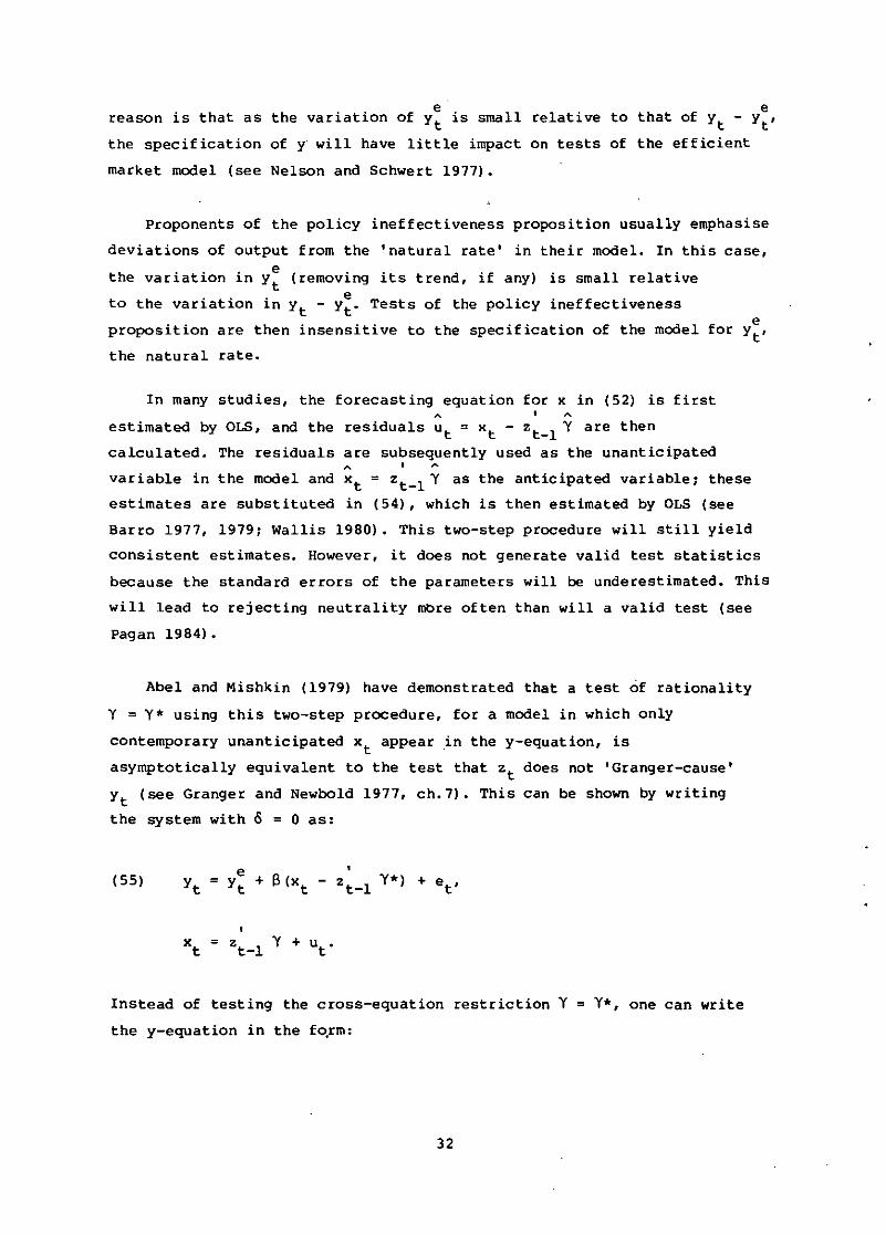
reason is that as the variation of y~ is small relative to
the spec if ication of y will have little impact on tests of
market model (see Nelson and Schwert 1977).
ethat of Yt - Yt'
the efficient
Proponents of the policy ineffectiveness proposition usually emphasise
deviations of output from the 'natural rate' in their model. In this case,
the variation in y~ (removing its trend, if any) is small relative
to the variation in Yt - y~. Tests of the policy ineffectivenesse
proposition are then insensitive to the specification of the model for Yt'
the natural rate.
~
variable in the model and K t ~ Zt_l Y as the anticipated variable: these
estimates are substituted in (54), which is then estimated by OLS (see
Barro 1977, 1979: Wallis 1980). This two-step procedure will still yield
In many studies, the forecasting equation for K in (52) is first~ ,~
estimated by OLS, and the residuals ut ~ K t - Zt_l Yare then
calculated. The residuals are subsequently used as the unanticipated, ~
consistent estimates. However, it does not generate valid test statistics
because the standard errors of the parameters will be underestimated. This
will lead to rejecting neutrality more often than will a valid test (see
Pagan 1984).
Abel and Mishkin (1979) have demonstrated that a test of rationality
y ~ y* using this two-step procedure, for a model in which only
contemporary unanticipated Kt
appear in the y-equation, is
asymptotically equivalent to the test that Zt does not 'Granger-cause'
Yt (see Granger and Newbold 1977, ch.7). This can be shown by writing
the system with 0 ~ 0 as:
( 55)
Instead of testing the cross-equation restriction Y ~ Y*, one can write
the y-equation in the fo~m:
32
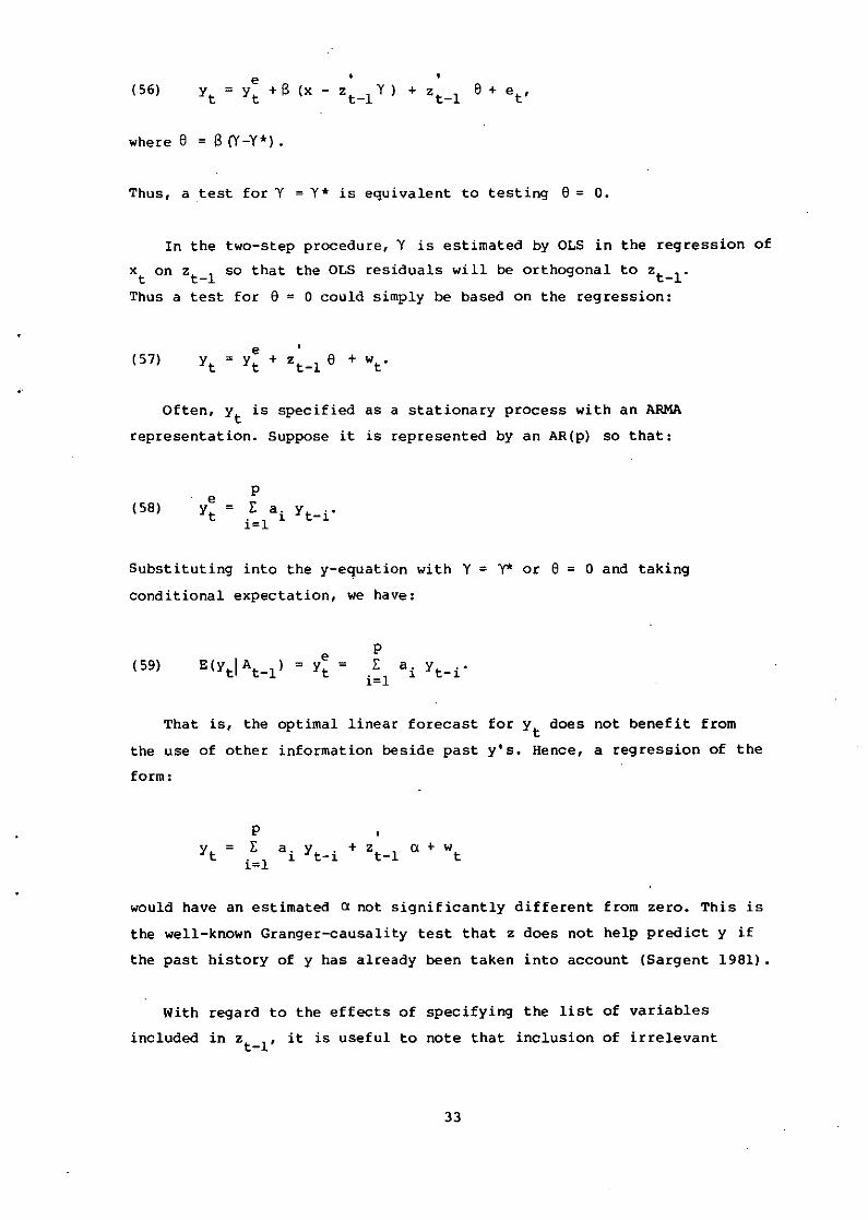
( 56)
where e = B (Y-y*) .
Thus, a test for Y = y* is equivalent to testing e = o.
In the two-step procedure, Y is estimated by OLS in the regression of
x on z 1 so that the OLS residuals will be orthogonal to Zt 1.t t- -
Thus a test for e = 0 could simply be based on the regression:
( 57)
Often, Yt is specified as a stationary process with an ARMA
representation. Suppose it is represented by an AR(p) so that:
(58)e p
Yt = E a. Yt-i.i=l 1
Substituting into the y-equation with Y = Y* or e = 0 and taking
conditional expectation, we have:
( 59)p
i:l a i Yt-i·
That is, the optimal linear forecast for Yt
does not benefit from
the use of other information beside past y's. Hence, a regression of the
form:
PE
i=la. Y + Z a + W
t1 t-i t-l
would have an estimated a not significantly different from zero. This is
the well-known Granger-causality test that z does not help predict y if
the past history of y has already been taken into account (Sargent 1981).
With regard to the effects of specifying the list of variables
included in Zt_l' it is useful to note that inclusion of irrelevant
33
predetermined variables will not lead to inconsistent parameter estimates
but will, in general, reduce the power of tests. On the other hand,
excluding relevant variables from Zt_l will lead to inconsistent
estimates of y. Even in this case, however, any rejection of the
constraint y = y. in (55) indicates a failure of rationality or of
neutrality, since a rejection of this constraint indicates that
Z 'Granger-causes' y. This shows that Luca~'s (1972) conjecture that tests
of neutrality cannot be conducted when there is a change in policy regime
(that is, new variables included in Zt_l) is not always correct.
Nevertheless, the change in policy regime could alter the variances of the
error terms and thus induce serial correlation or heteroscedasticity,
rendering the tests invalid.
Sargent (1973, 1976) pointed out that the Granger-causality tests are
valid tests of neutrality (0 = 0) and rationality (that is, Y = y.) ife(a) lagged values of xt - xt do not enter the y-equation (60) or (b) the
error term et is serially uncorrelated. The result breaks down if there
are lagged surprises (x t - x~) in (55) because the lagged OLS residuals
from the x-equation are not orthogonal to Zt_l. The Granger causality
test will no longer be a test of the hypotheses of rationality and/or
neutrality. In this case, the only valid test will be generated by
estimating both the x-equation and the y-equation jointly with and without
imposing the cross-equation restrictions and using the likelihood ratio
test.
Startz (1983) has considered Wald-type tests for the cross-equation
restr ictions.
7. THE LUCAS' CRITIQUE OF CONVENTIONAL ECONOMETRIC POLICY EVALUATION
The conventional approach to econometric policy evaluation is to take an
estimated model assuming an invariant structure. The implied reduced form
from the model is then used to predict the behaviour of the endogenous
variables under alternative specifications of the future values of policy
instruments (exogenous variables). Lucas (1976) criticises such
comparisons of alternative policy rules on the ground that the 'structure'
of econometric models - hence the implied reduced form - is not invariant
to changes in policy. For such comparisons to be meaningful, it is
34
•
necessary to assume that the nature of the economic system's reponse is
unaltered when substantial shifts in key variables occur.
Sims (1980) has also defined a structural model as one in which the
parameters can be treated as fixed over the relevant range of potential
changes in the policy rule. Some parameters of a model could be made
structural through the use of REH while other parameters were made
structural by assumption.
If adaptive expectations were used, then the coefficients of
expectation would not be policy-invariant and hence would not' be
structural. The shortcoming with these expectational assumptions is the
failure to take full account of agents' reaction to the policies
formulated. The 'problem is characteristic of both policy simulation and
formal optimal control techniques, each of which is based on the reduced
form model in which expectations are formed by fixed-coefficient
distributed lag structures. Since these lag structures show no direct
relationship to government policy, the mechanisms generating expectations
are inconsistent with those that take account of this policy.
Attempts to revise the methodology along the lines suggested by Lucas
appear to have been frustrated by the Sargent and Wallace proposition of
policy ineffectiveness under REH. However, when it was discovered that the
negative result relied heavily on a specialised structure rather than on
REH as such, the Lucas criticism was finally accepted as being
constructive rather than destructive.
The modern approach would now distinguish an underlying economic
structure incorporating the REH from a forecasting mechanism for the
exogenous policy rule which is allowed to change as policy changes.
The contribution of the Lucas critique tq econometric methodology is
now recognised as a breakthrough comparable to that of the Cowles
Commission who, in the 1950s, suggested that in policy analysis structural
simultaneous equations rather than single-equation reduced forms should be
modelled, to avoid bias. More care should now be devoted to modelling
expectations that are consistent with the model structure.
35
8. CONCLUSION
The rational expectations hypothesis takes into account the important case
of endogenous expectations formation, as was foreshadowed by Keynes in his
General Theory. While the hypothesis has generally been accepted as being
more plausible than the ad hoc approach in forming expectations, RE models
cannot guarantee to deliver unique solutions and replicate the real world.
However, if the real world is characterised by expectational confusion,
then the RE model reveals this problem and thus leads to better policies
which avoid it.
Regarding the problem of identification, economists cannot implement
the RE solution unless the structural parameters can be disentangled from
economic data. Even if the parameters are identified, individuals may have
begun from an incorrect view of the economy, forming mistaken expectations
which cause the RE model to fail to replicate reality. However, if
individuals do not make perceivable errors in forecasting the future, then
the RE hypothesis is a convenient assumption with which to begin the
analysis of endogenous expectations formation.
The idea that policy changes may induce revision of individuals'
behaviour dates back to Marschak (1953). Macroeconomic analysis of
stabilisation policy· should recognise that individuals' expectations are
endogenous, depending on the operation of government policies, as pointed
out by Lucas. What remains to be studied is how to capture more accurately
the constraints which intertemporal decision makers actually face, and to
model more realistically the information they can acquire when forming
expectations (see Blanchard 1981).
This new mode of thinking among economists has led to SUbstantial
progress in the analysis of bond and foreign exchange markets. BY
emphasising the dangers of ad hoc expectations rules, the RE approach has
encouraged a more general reconsideration of the micro foundation of
macroeconomics •
. Most of the early empirical literature uses 'limited information'
estimation of equations. Since REH imposes precise cross-equation
restrictions, this information concerning the full system should be
36
imposed a priori to obtain more efficient es~imates and more powerful
tests. The Lucas problem must also be addressed. A forecast or simulation
should involve a series of iterations until the evolution of the economy
is consistent with the expectations the model assumes.
Further insights concerning rational expectations theory may be found
in the works of Taylor (1985), Begg (1982), Mishkin (1983) and Sheffrin
(1983).
37
REFERENCES
Abel, A. and F.S. Mishkin (1979),On the Econometric Testing of Rationality
and Market Efficiency, Chicago Report No. 7933, University of Chicago.
Anderson, G.J., Pearce, I.F. and Trivedi, P.K. (1976), 'Output, expected
demand and unplanned stocks' in I.F. Pearce et al. (eds) , A Model of
Output, Employment, Wages and Prices in the United Kingdom, Cambridge
University Press, Cambridge.
Aoki, M. and Canzoneri, M. (1979), 'Reduced forms of rational expectations
models', The Quarterly Journal of Economics 93, 59-71.
Barro, R.J. (1977), 'Unanticipated money growth and unemployment in the
United States', American Economic Review 67, 101-15.
___ (1979) ,'Unanticipated money growth and unemployment in the United
States: reply'. American Economic Review 69, 1004-9.
Begg, D.K.H. (1982), The Rational Expectations Revolution in
Macroeconomics, Philip Allan, Oxford.
Bernanke, B. (1982), The financial collapse as a direct cause of the Great
Depression. Stanford University Graduate School of Business, California
(unpubli shed) •
Blanchard, O.J. (1979), 'Backward and forward solutions for economies with
rational expectations', American Economic Review 69, 114-8.
___ (1981), 'Output, the stock market, and interest rates', American
Economic Review 71, 132-43.
Box, G.E.P. and Jenkins, G.M. (1970), Time Series Analysis, Forecasting
and Control, Holden Bay, San Francisco.
Border, K.C. and Jordan, J.S. (1979), 'Expectations equilibrium with
expectations based on past data', Journal of Economic Theory 22, 395-406.
38
•Suiter, W.H. (1980), Real effects of anticipated and unanticipated money:
some problems of estimation and hypothesis testing. Working Paper No.
601, National Bureau of Economic Research, Cambridge, Massachusetts.
Cagan, P. (1956), 'The monetary dynamics of hyper-inflation' in M.
Friedman (ed.), Studies in the Quantity Theory of Money, University of
Chicago Press, Chicago.
Chow, G.C. (1983), Econometrics, McGraw-Hill, New York.
Coase, R.H. and Fowler, R.F. (1935), 'Bacon production and the pig cycle
in Great Britain', Economica, 2, 142-67.
Debreu, G. (1959), Theory of Value, Wiley, New York.
Dornbusch, R. (1976), 'Expectations and exchange rate dynamics', Journal
of Political Econo~ 84, 1161-76.
Duck, N., Parkin, M., Rose, D. and Zis, G. (1976), 'The determination of
the rate of change in wages and prices in the fixed exchange rate world
economy, 1956-1971' in M. Parkin and G. zis (eds) , Inflation in the
World Economy, Manchester University Press, Manchester, United Kingdom.
Fair, R. and Taylor, J.B. (1983), 'Solution and maximum likelihood
estimation of dynamic non-linear rational expectations models',
Econometrica 51, 1169-85.
Fisher, F.M. (1966), The Identification Problem, McGraw-Hill, New York.
Frenkel, J.A. (1981), 'The collapse of purchasing power parity during the
1970s', European Economic Review 16, 145-65.
Futia, C.A. (1981) 'Rational expectations in stationary linear models',
Econometrica 49, 171-92.
Granger, C.W.J. and Newbold, P. (1977), Forecasting Economic Time Series
Academic Press, New York.
39
Grossman, J. (1979), 'Nominal demand policy and short-run fluctuations in
unemployment and prices in the United States', Journal of Political
Economy 87, 1063-85.
Hansen, L.P. and Singleton, K.J. (1982), 'Generalised instrumental
variables estimation of non-linear rational expectations models',
Econometrica 50, 1269-86.
Jordan, J.S. (1980), 'On the predictability of economic events',
Econometrica 48, 955-86.
Kantor, B. (1979), 'Rational expectations and economic thought', Journal of
Economic Literature 17, 1422-41.
Keynes, J.M. (1936) The General Theory of Employment Interest and Money,
Macmillan, London.
Lucas, R.E. (1972), 'Expectations and the neutrality of money', Journal of
Economic Theory 4, 103-4.
___ (1976), 'Econometric policy evaulation: a critique', in K. Brunner and
A.H. Meltzer (eds) , The Phillips Curve and Labour Markets,
Carnegie-Rochester Conference Series, No.1, North Holland, New York,
19-46.
___ and Sargent, T.J. (1978), 'After Keynesian macro-economics' in After
the Phillips Curve: Persistence of High inflation and High Unemployment,
Federal Reserve Bank of Boston, Massachusetts.
Marschak, J. (1953), 'Economic measurements for policy and prediction',
W.C. Hood and T.C. Koopmans (eds) , Studies in Econometric Methods, Yale
University Press, Connecticut.
Metzler, L. (1941), 'The nature and stability of inventory cycles', Review
of Economics and Statistics 3, 113-29.
40
"
.'
Mccallum, B.T. (1976a), 'Rational expectations and the estimation of
economists' models: an alternative procedure', International Economic
Review 17, 484-90.
(1976b), 'Rational expectations and the natural rate hypothesis: some
consistent estimates', Econometrica 44, 43-52.
___ (1983), 'On non-uniqueness in rational expectations: an attempt at
perspective', Journal of Monetary Economics II, 139-68.
Mishkin, F.S. (1983) A Rational Expectations Approach to Macroeconometrics,
National Bureau of Economic Research Monograph, University of Chicago
Press, Chicago.
Muth, J.F. (1961), 'Rational expectations and the theory of price
movements', Econometrics 29, 315-35.
Nelson, C.R. and Schwert, G.w. (1977), 'Short term interest rates as
predictors of inflation: on testing the hypothesis that the real rate is
constant', American Economic Review 67, 475-86.
Nerlove, M. (1958), 'Adaptive expectations and cobweb phenomena', Quarterly
Journal of Economics 72, 227-40.
Pagan, A. (1984), 'Econometric issues in the analysis of regressions with
generalised regressors', International Economic Review 25, 221-48.
pesaran, M.H. (1981), 'Identification of rational expectations models',
Journal of Econometrics 16, 375-98.
Radner, R. (1982), 'Equilibrium under uncertainty', in K.J. Arrow and
M.D. Intriligator (eds), Handbook of Mathematical Economics, Vol. II,
North Holland, Amsterdam.
Revankar, N.S. (1980), 'Testing of the rational expectations hypothesis',
Econometrica 48, 1347-63.
41
Rothenberg R.J. (1973), Efficient Estimation with A Priori Information,
Cowles Foundation Monograph No. 23, Yale University press, Connecticut.
Saracoglu,·R. and Sargent, T.J. (1978), 'seasonality and portfolio balance
under rational expectations', Journal of Monetary Economics 4, 435-54.
Sargent, T.J. (1973), 'Rational expectations, theoretical rate of interest,
and the natural rate of unemployment', Brookings Papers on Economic
Activity 2, 429-72.
___ (1976), 'The observational equivalence of natural and unnatural rate
theories of macroeconomics', Journal of Political Economy 84, 631-640.
___ (1979), Macroeconomic Theory, Academic Press, New York.
___ (1981), 'Interpreting economic time series', Journal of Political
Economy 89, 213-48.
___ and Wallace, N. (1975), 'Rational expectations, the optimal monetary
instrument and the optimal money supply rule', Journal of Political
Economy 83, 241-54.
___ and (1976), 'Rational expectations and the theory of economic
policy', Journal of Monetary Economics 2, 169-83.
Sheffrin, S. (1979), 'Unanticipated monetary growth and output
fluctuations', Economic Inquiry 17, 1-13.
___ (1983), Rational Expectations, Cambridge University Press, United
Kingdom.
Shiller R.J. (1978), 'Rational expectations and the dynamic structure of
macroeconomic models', Journal of Monetary Economics 4,1-44.
___ (1980), 'Can the Fed control real interest rates?' in S. Fisher (ed.) ,
Rational Expectations and Economic Policy, University of Chicago Press,
Chicago.
42
•
,
•
•
Sims, C.A. (1980), 'Macroeconomics and reality', Econometrica 48, 1-48.
Startz, R. (1983), 'Testing rational expectations by the use of
overidentifying restrictions', Journal of Econometrics 23; 343-51.
Taylor, J.B. (1977), 'On conditions for unique solutions in stochastic
macroeconomic models with price expectations', Econometrica 45, 1377-86.
(1985), 'New econometric techniques for macroeconomic policy
evaluation' in Z. Griliches and M.D. Intriligator (eds), Handbook of
Econometrics, Vol. 3, North Holland, Amsterdam.
Wallis, K.F. (1980), 'Econometric implications of the rational expectations
hypothesis', Econometrica 48, 49-72.
Wegge, L.L. and M. Feldman (1983), 'Identifiability criteria for
Muth-rational expectations models', Journal of Econometrics 21, 245-54.
Whiteman, C.H. (1983), Linear Rational Expectations Models: A Users Guide,
University of Minnesota Press, Minneapolis.
Wickens, M.R. (1982), 'The efficient estimation of econometric models with
rational expectations', Review of Economic Studies 49, 55-68 •
43