TOPICS IN ADVANCED ECONOMETRICS: SVAR

MODELS

PART I

LESSON 3

Luca Fanelli

University of Bologna

luca.fanelli@unibo.it

http://www.rimini.unibo.it/fanelli

The material in these slides is based on the following

books and papers:

— Amisano, G., Giannini, C. (1997), Topics in Struc-

tural VAR Econometrics,

Springer.

— Hamilton, J.D. (1994), Time Series Analysis, Prince-

ton University Press.

— Lutkepohl, H. (2006), New Introduction to Multiple

Time Series Analysis, Berlin: Springer-Verlag, 2006.

— Pesaran, M. H., Shin, Y. (1998), Generalized Im-

pulse Response Analysis in Linear Multivariate Mod-

els, Economic Letters 58, 17-29.

— Personal processing.

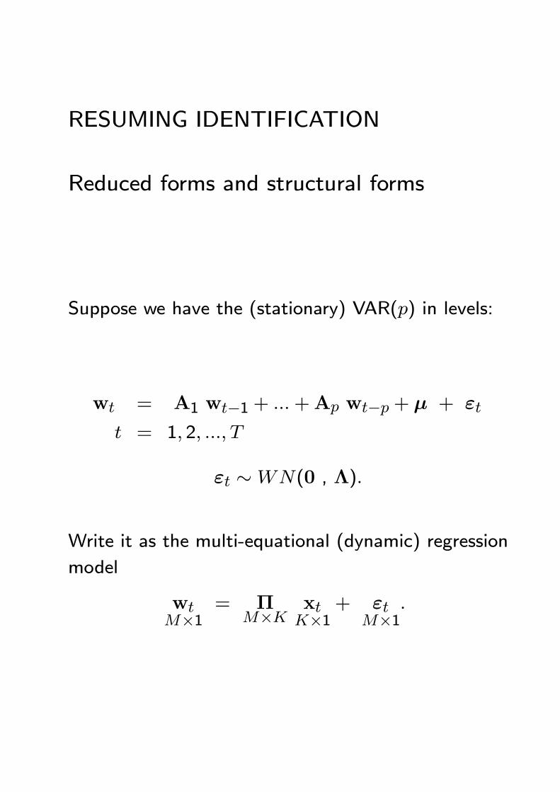
RESUMING IDENTIFICATION

Reduced forms and structural forms

Suppose we have the (stationary) VAR(p) in levels:

wt = A1 wt−1 + ...+Ap wt−p + µ + εt

t = 1, 2, ..., T

εt ∼WN(0 , Λ).

Write it as the multi-equational (dynamic) regression

model

wtM×1

= ΠM×K xt

K×1+ εt

M×1.

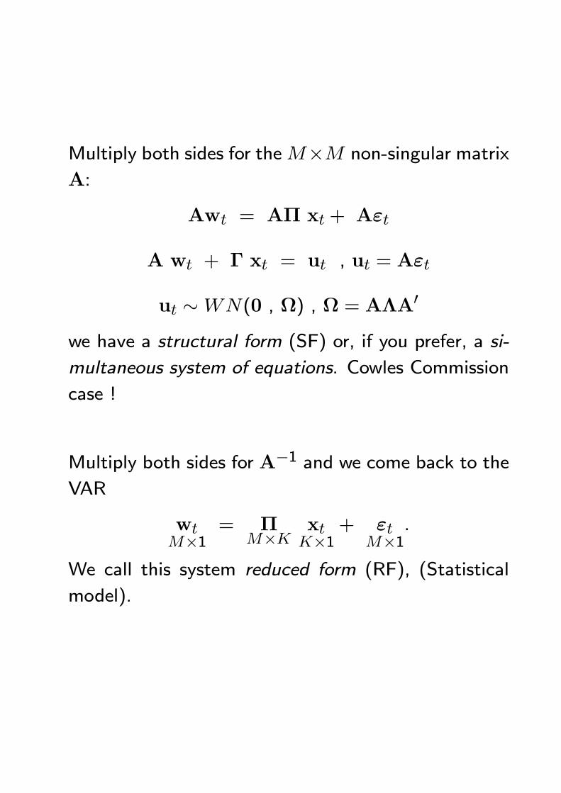
Multiply both sides for theM×M non-singular matrix

A:

Awt = AΠ xt + Aεt

A wt + Γ xt = ut , ut = Aεt

ut ∼WN(0 , Ω) , Ω = AΛA0

we have a structural form (SF) or, if you prefer, a si-

multaneous system of equations. Cowles Commission

case !

Multiply both sides for A−1 and we come back to theVAR

wtM×1

= ΠM×K xt

K×1+ εt

M×1.

We call this system reduced form (RF), (Statistical

model).

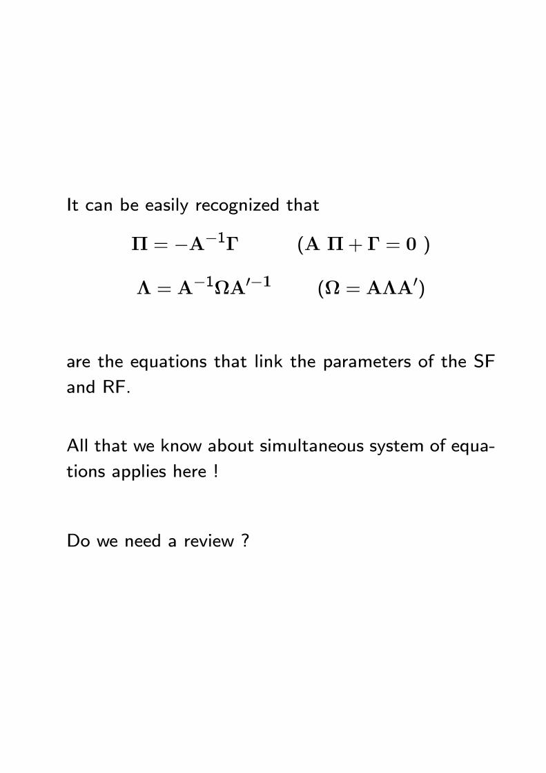
It can be easily recognized that

Π = −A−1Γ (A Π+ Γ = 0 )

Λ = A−1ΩA0−1 (Ω = AΛA0)

are the equations that link the parameters of the SF

and RF.

All that we know about simultaneous system of equa-

tions applies here !

Do we need a review ?

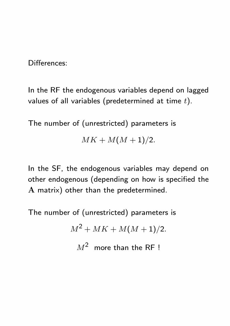
Differences:

In the RF the endogenous variables depend on lagged

values of all variables (predetermined at time t).

The number of (unrestricted) parameters is

MK +M(M + 1)/2.

In the SF, the endogenous variables may depend on

other endogenous (depending on how is specified the

A matrix) other than the predetermined.

The number of (unrestricted) parameters is

M2 +MK +M(M + 1)/2.

M2 more than the RF !

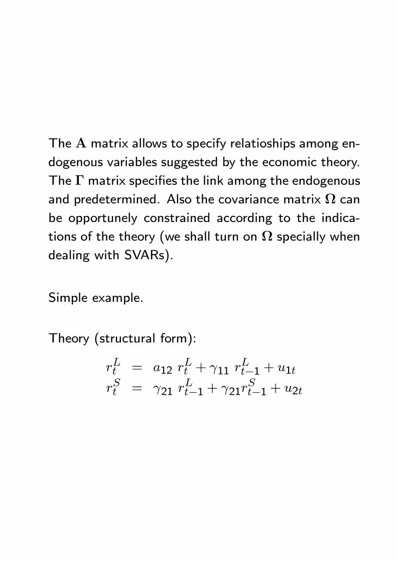
The A matrix allows to specify relatioships among en-

dogenous variables suggested by the economic theory.

The Γ matrix specifies the link among the endogenous

and predetermined. Also the covariance matrix Ω can

be opportunely constrained according to the indica-

tions of the theory (we shall turn on Ω specially when

dealing with SVARs).

Simple example.

Theory (structural form):

rLt = a12 rLt + γ11 r

Lt−1 + u1t

rSt = γ21 rLt−1 + γ21r

St−1 + u2t

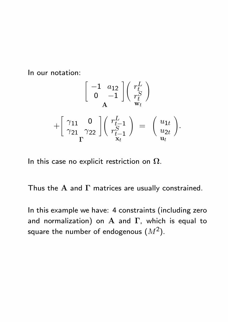
In our notation: "−1 a120 −1

#A

ÃrLtrSt

!wt

+

"γ11 0γ21 γ22

#Γ

ÃrLt−1rSt−1

!xt

=

Ãu1tu2t

!ut

.

In this case no explicit restriction on Ω.

Thus the A and Γ matrices are usually constrained.

In this example we have: 4 constraints (including zero

and normalization) on A and Γ, which is equal to

square the number of endogenous (M2).

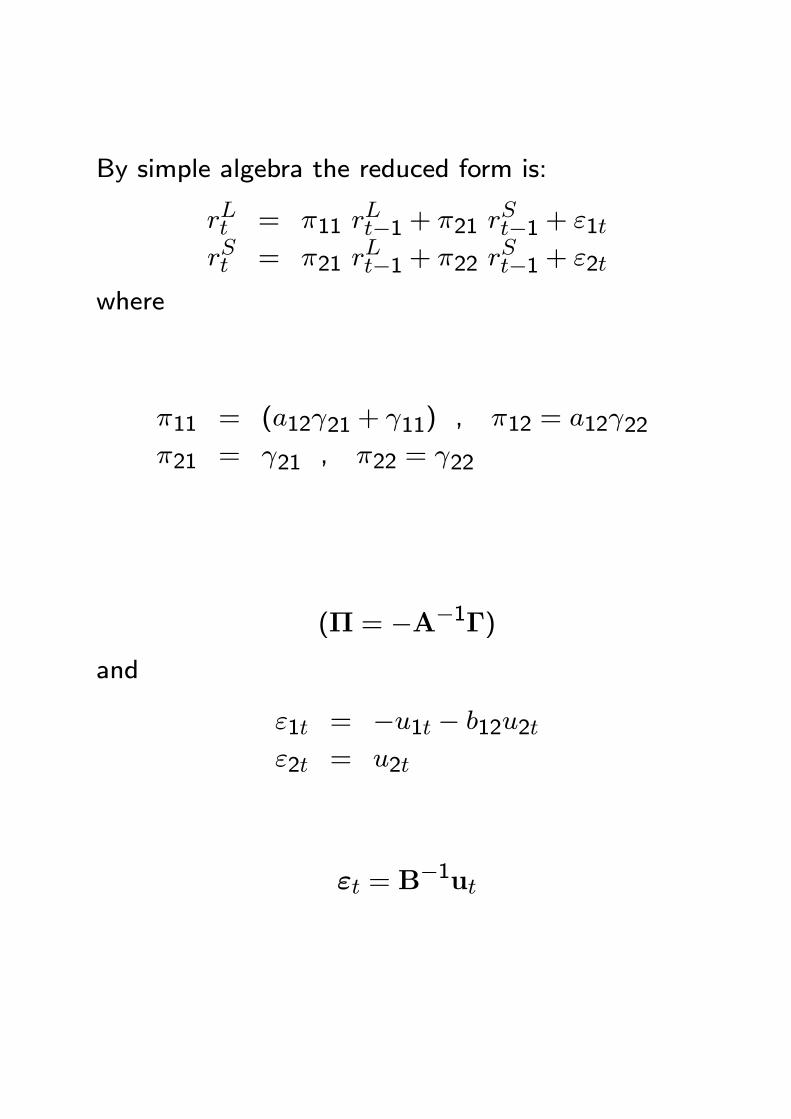
By simple algebra the reduced form is:

rLt = π11 rLt−1 + π21 r

St−1 + ε1t

rSt = π21 rLt−1 + π22 r

St−1 + ε2t

where

π11 = (a12γ21 + γ11) , π12 = a12γ22π21 = γ21 , π22 = γ22

(Π = −A−1Γ)and

ε1t = −u1t − b12u2tε2t = u2t

εt = B−1ut

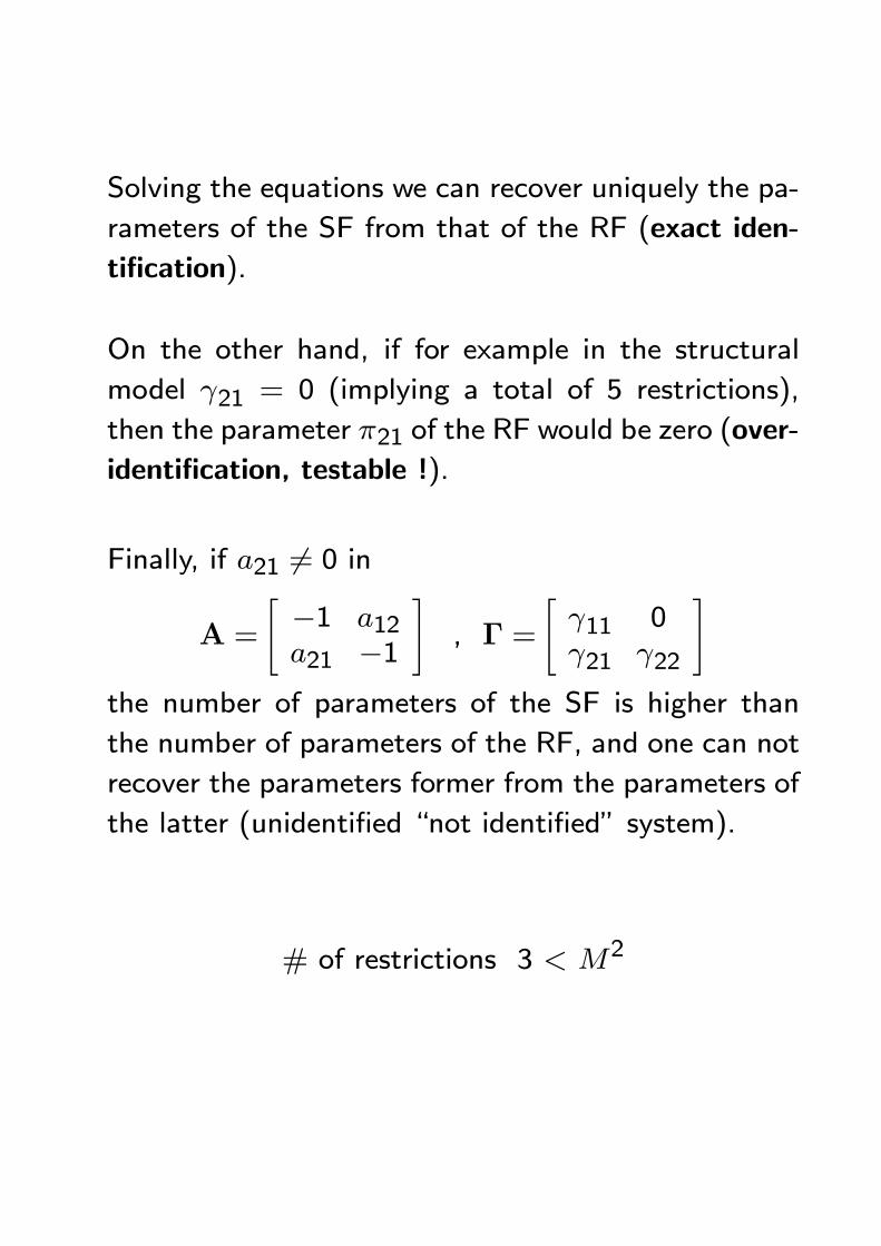
Solving the equations we can recover uniquely the pa-

rameters of the SF from that of the RF (exact iden-

tification).

On the other hand, if for example in the structural

model γ21 = 0 (implying a total of 5 restrictions),

then the parameter π21 of the RF would be zero (over-

identification, testable !).

Finally, if a21 6= 0 in

A =

"−1 a12a21 −1

#, Γ =

"γ11 0γ21 γ22

#the number of parameters of the SF is higher than

the number of parameters of the RF, and one can not

recover the parameters former from the parameters of

the latter (unidentified “not identified” system).

# of restrictions 3 < M2

Identification problem in general

In short, we known that if f(w1, w2, ..., wT ; θ) is the

likelihood function, we require a 1-1 mapping between

the elements θ ∈ Ξ, and the probability distribution

of observations.

In other words, if θ1∈ Ξ and θ2∈ Ξ we expect that

f(w1,w2, ...,wT ;θ1) 6= f(w1,w2, ...,wT ;θ2)

otherwise θ1 and θ2 would be observationally equiv-

alent. In many circumstances we are able to discuss

identification only in a neighborhood of the “true”

parameters values (local identifiability).

Recall from previous lesson that:

lnL(θ) = log f(w1, w2, ..., wT ; θ)

Hessian: H(θ) = ∂2 lnL(θ)∂θ∂θ0

Sample information matrix:

IT (θ) = E

Ã−∂

2 lnL(θ)

∂θ∂θ0

!, IT (θ0) full rank

Suppose that in our model:

εt ∼WNN(0,Λ) , ut ∼WNN(0 , Ω) , Ω = AΛA0.

The log-likelihood of the SF is then given by

lnL(A, Γ, Ω) = C+T log | det(A) | −(T/2) log(det(Ω))

−12

TXt=1

(Ayt + Γxt)0Ω−1(Ayt + Γxt)

where C is a constant.

Why ?

We known that for two given random vectors w and

u of suitable dimensions such that

wM×1 = g( u

M×1)

and g(·) invertible, it holds:fw(w) = fu(g

−1(w)) × | det[∂g−1(w)/∂w0] |where ∂g−1(w)/∂w0 is the M ×M Jacobian matrix.

Start form ut ∼WNN(0 , Ω) , hence

fη(ut , Ω) = (2π)−M/2 det(Ω)−1/2 exp

−12

TXt=1

u0tΩ−1ut

Since

wt = Πxt + A−1utit exists a linear relation between wt and ut of the

form: wt = g(ut). It is also true that ut = g−1(wt)

and that ∂ut/∂w0t = A.

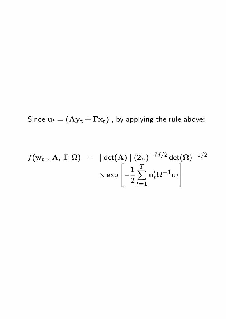
Since ut = (Ayt + Γxt) , by applying the rule above:

f(wt , A, Γ Ω) = | det(A) | (2π)−M/2 det(Ω)−1/2

× exp−12

TXt=1

u0tΩ−1ut

Now consider the SF given by the parameters

(A∗, Γ∗, Ω∗), where

A∗ = A0A, Γ∗ = A0Γ, Ω∗ = A0ΩA00

and A0 is (M ×M) non-singular.

Both (A, Γ, Ω) and (A∗, Γ∗, Ω∗) belong to the spaceof parameters of the SF and it can be easily recognized

that

lnL(A,Γ,Ω) = lnL(A∗,Γ∗,Ω∗)

i.e. (A, Γ, Ω) and (A∗, Γ∗, Ω∗) are observationallyequivalent.

The identification problem does not arise in the RF.

That is the RF is identified by construction.

It is the SF which is generally not identifiable due

to the presence of simultaneous relations through the

A matrix .... unless a given number of identifying

constraints is imposed on (A, Γ, Ω) (observe that

the number of parameters of the SF is higher than

the RF).

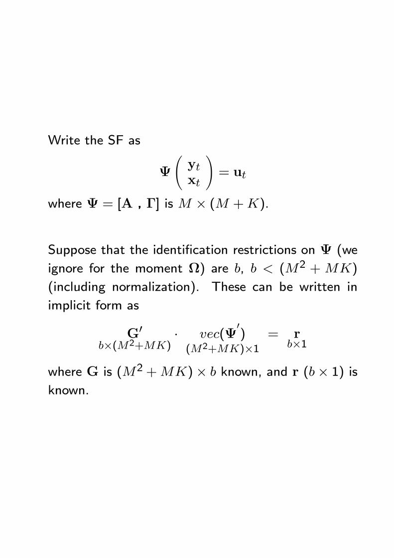
Write the SF as

Ψ

Ãytxt

!= ut

where Ψ = [A , Γ] is M × (M +K).

Suppose that the identification restrictions on Ψ (we

ignore for the moment Ω) are b, b < (M2 +MK)

(including normalization). These can be written in

implicit form as

G0b×(M2+MK)

· vec(Ψ0)

(M2+MK)×1= r

b×1

where G is (M2 +MK)× b known, and r (b× 1) isknown.

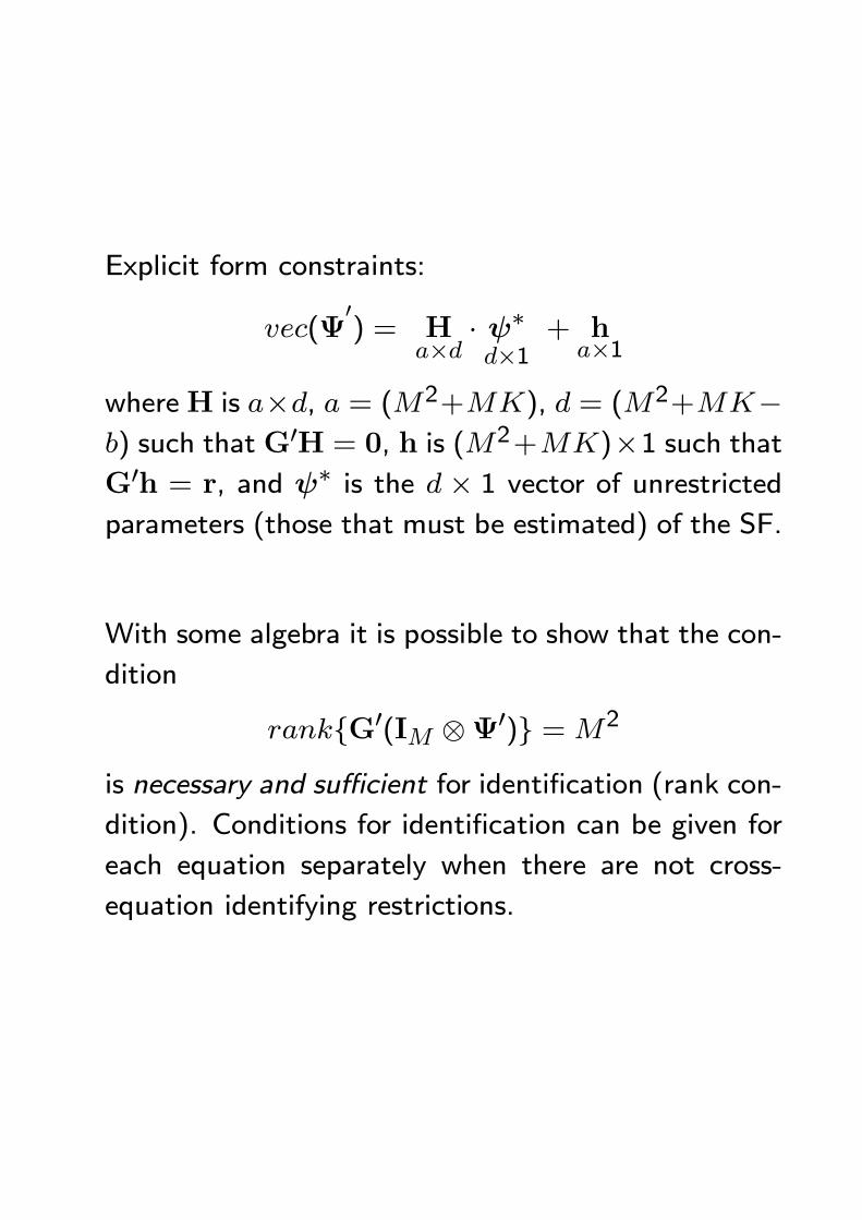
Explicit form constraints:

vec(Ψ0) = H

a×d · ψ∗

d×1+ h

a×1

whereH is a×d, a = (M2+MK), d = (M2+MK−b) such that G0H = 0, h is (M2+MK)×1 such thatG0h = r, and ψ∗ is the d × 1 vector of unrestrictedparameters (those that must be estimated) of the SF.

With some algebra it is possible to show that the con-

dition

rankG0(IM ⊗Ψ0) =M2

is necessary and sufficient for identification (rank con-

dition). Conditions for identification can be given for

each equation separately when there are not cross-

equation identifying restrictions.

From this it follows that

b ≥M2

is only necessary for identification (order condition).

(When b > M2 the system is over-identified; over-

identification entails that the parameters of the RF are

subject to (b−M2) restrictions that must be tested).

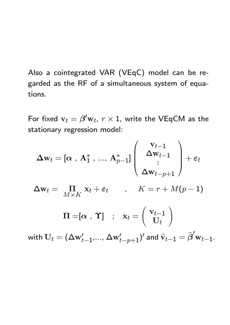
Also a cointegrated VAR (VEqC) model can be re-

garded as the RF of a simultaneous system of equa-

tions.

For fixed vt = β0wt, r × 1, write the VEqCM as the

stationary regression model:

∆wt = [α , A∗1 , ..., A∗p−1]

vt−1

∆wt−1...

∆wt−p+1

+ εt

∆wt = ΠM×K xt + εt , K = r +M(p− 1)

Π =[α , Υ] ; xt =

Ãvt−1Ut

!

withUt = (∆w0t−1,...,∆w0t−p+1)0 and bvt−1 = bβ0wt−1.

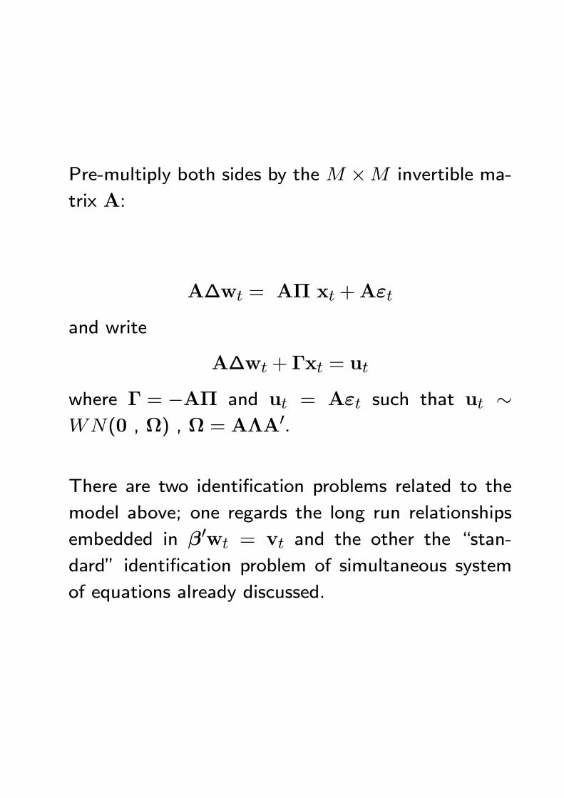
Pre-multiply both sides by the M ×M invertible ma-

trix A:

A∆wt = AΠ xt +Aεt

and write

A∆wt + Γxt = ut

where Γ = −AΠ and ut = Aεt such that ut ∼WN(0 , Ω) , Ω = AΛA0.

There are two identification problems related to the

model above; one regards the long run relationships

embedded in β0wt = vt and the other the “stan-

dard” identification problem of simultaneous system

of equations already discussed.

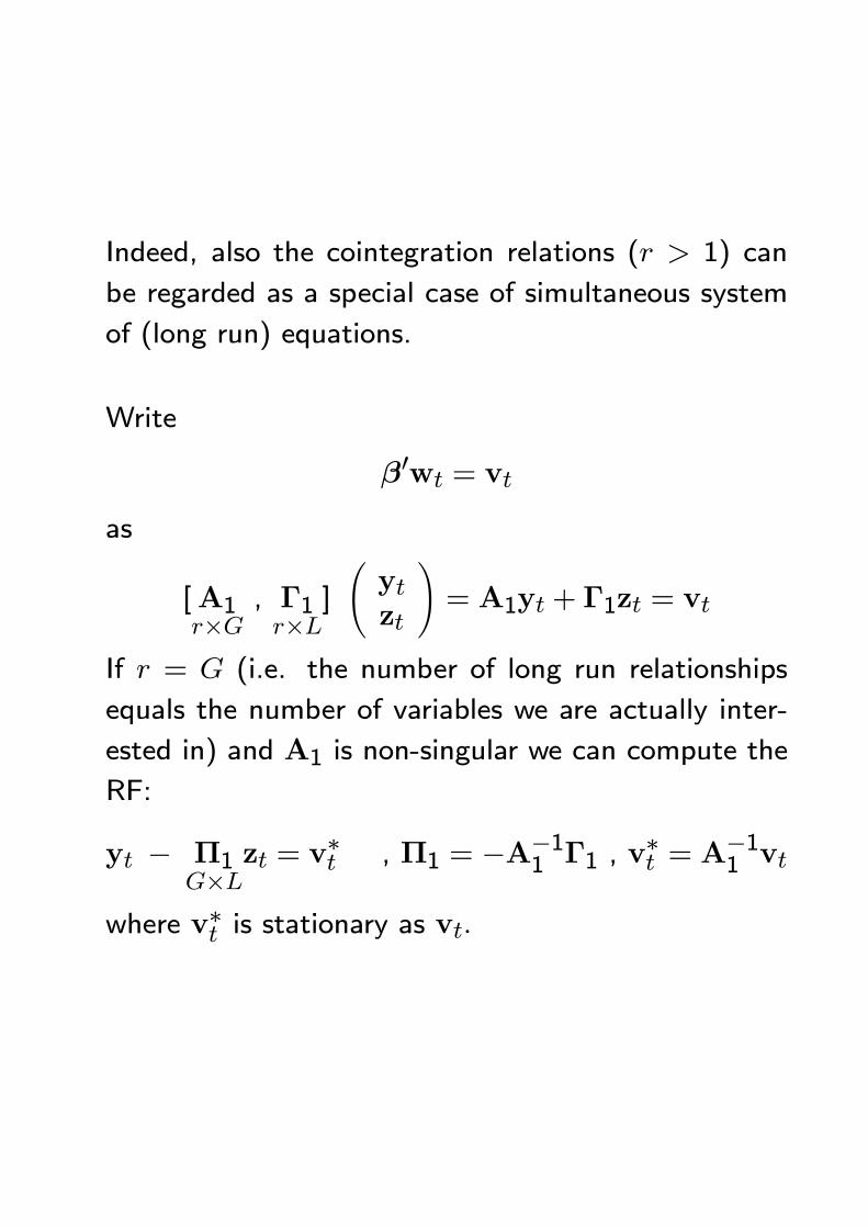
Indeed, also the cointegration relations (r > 1) can

be regarded as a special case of simultaneous system

of (long run) equations.

Write

β0wt = vt

as

[A1r×G

, Γ1r×L

]

Ãytzt

!= A1yt + Γ1zt = vt

If r = G (i.e. the number of long run relationships

equals the number of variables we are actually inter-

ested in) and A1 is non-singular we can compute the

RF:

yt − Π1G×L

zt = v∗t , Π1 = −A−11 Γ1 , v

∗t = A

−11 vt

where v∗t is stationary as vt.

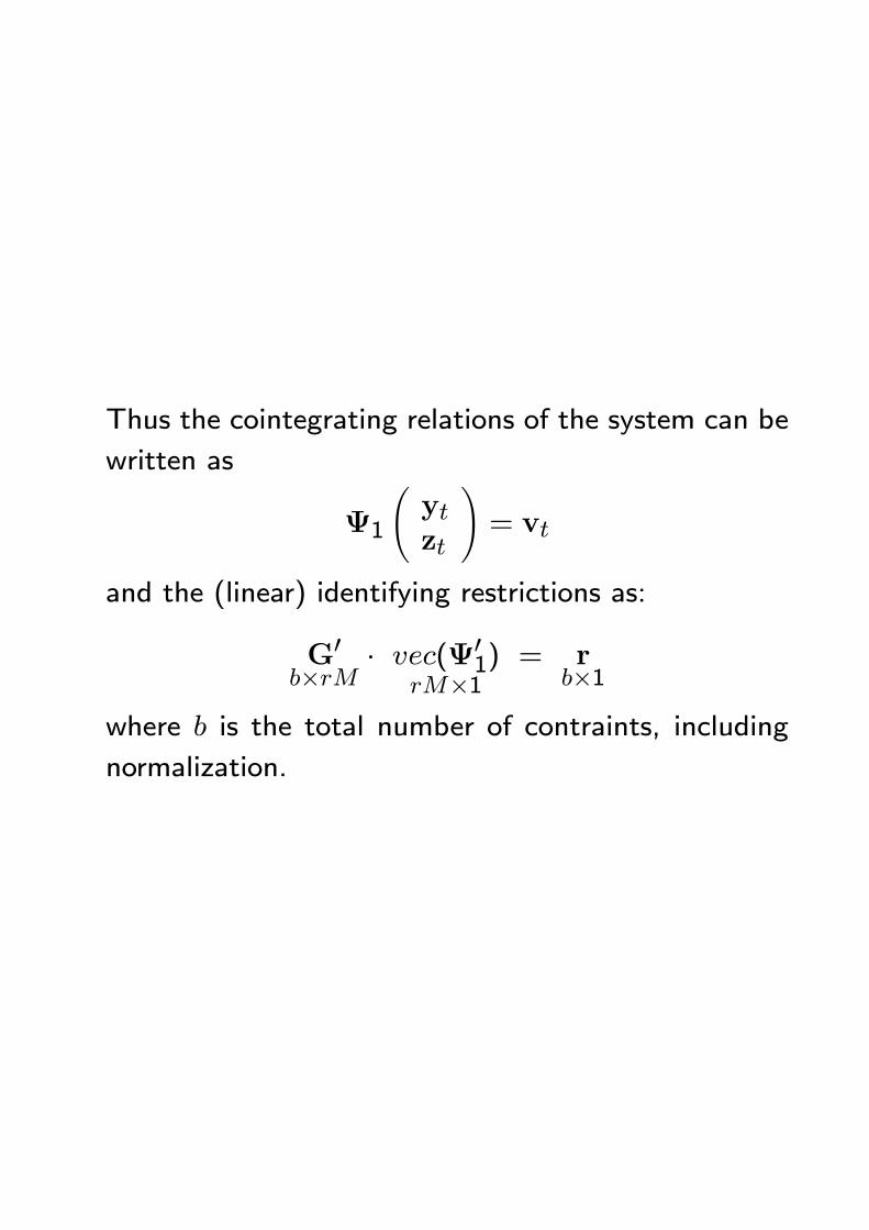
Thus the cointegrating relations of the system can be

written as

Ψ1

Ãytzt

!= vt

and the (linear) identifying restrictions as:

G0b×rM · vec(Ψ01)

rM×1= r

b×1where b is the total number of contraints, including

normalization.

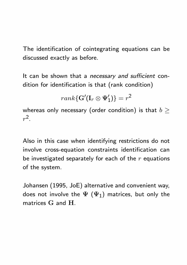
The identification of cointegrating equations can be

discussed exactly as before.

It can be shown that a necessary and sufficient con-

dition for identification is that (rank condition)

rankG0(Ir ⊗Ψ01) = r2

whereas only necessary (order condition) is that b ≥r2.

Also in this case when identifying restrictions do not

involve cross-equation constraints identification can

be investigated separately for each of the r equations

of the system.

Johansen (1995, JoE) alternative and convenient way,

does not involve the Ψ (Ψ1) matrices, but only the

matrices G and H.

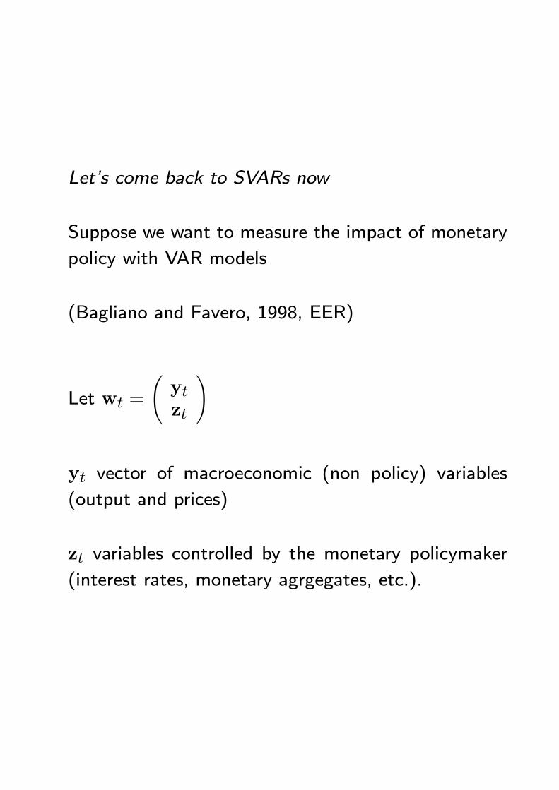
Let’s come back to SVARs now

Suppose we want to measure the impact of monetary

policy with VAR models

(Bagliano and Favero, 1998, EER)

Let wt =

Ãytzt

!

yt vector of macroeconomic (non policy) variables

(output and prices)

zt variables controlled by the monetary policymaker

(interest rates, monetary agrgegates, etc.).

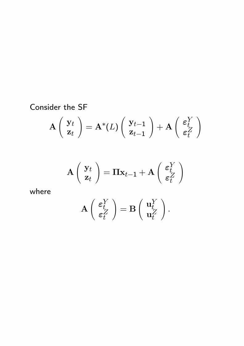
Consider the SF

A

Ãytzt

!= A∗(L)

Ãyt−1zt−1

!+A

ÃεYtεZt

!

A

Ãytzt

!= Πxt−1 +A

ÃεYtεZt

!where

A

ÃεYtεZt

!= B

ÃuYtuZt

!.

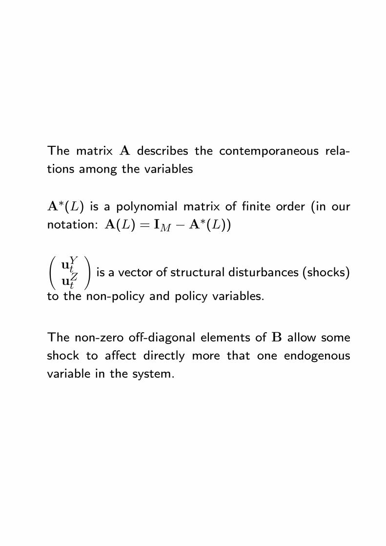
The matrix A describes the contemporaneous rela-

tions among the variables

A∗(L) is a polynomial matrix of finite order (in ournotation: A(L) = IM −A∗(L))

ÃuYtuZt

!is a vector of structural disturbances (shocks)

to the non-policy and policy variables.

The non-zero off-diagonal elements of B allow some

shock to affect directly more that one endogenous

variable in the system.

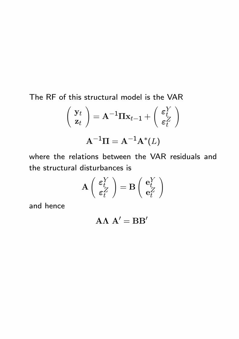
The RF of this structural model is the VARÃytzt

!= A−1Πxt−1 +

ÃεYtεZt

!

A−1Π = A−1A∗(L)

where the relations between the VAR residuals and

the structural disturbances is

A

ÃεYtεZt

!= B

ÃeYteZt

!and hence

AΛ A0 = BB0

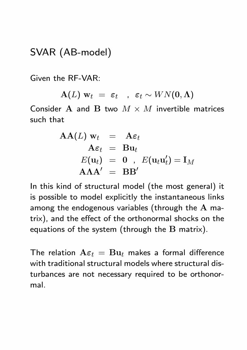
SVAR (AB-model)

Given the RF-VAR:

A(L) wt = εt , εt ∼WN(0,Λ)

Consider A and B two M × M invertible matrices

such that

AA(L) wt = AεtAεt = But

E(ut) = 0 , E(utu0t) = IM

AΛA0 = BB0

In this kind of structural model (the most general) it

is possible to model explicitly the instantaneous links

among the endogenous variables (through the A ma-

trix), and the effect of the orthonormal shocks on the

equations of the system (through the B matrix).

The relation Aεt = But makes a formal differencewith traditional structural models where structural dis-

turbances are not necessary required to be orthonor-

mal.

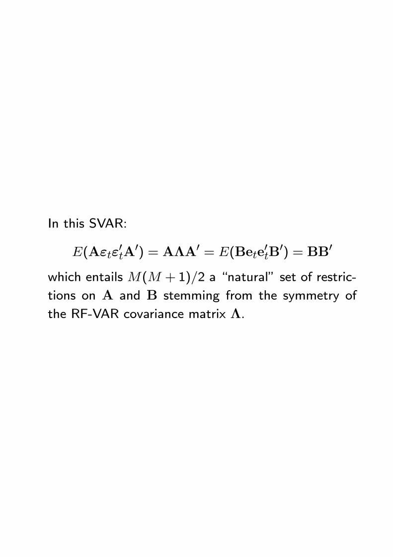
In this SVAR:

E(Aεtε0tA0) = AΛA0 = E(Bete

0tB0) = BB0

which entails M(M +1)/2 a “natural” set of restric-

tions on A and B stemming from the symmetry of

the RF-VAR covariance matrix Λ.

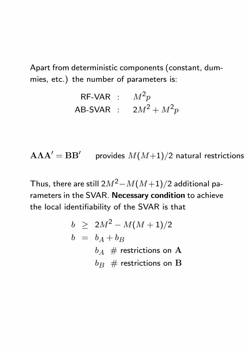
Apart from deterministic components (constant, dum-

mies, etc.) the number of parameters is:

RF-VAR : M2p

AB-SVAR : 2M2 +M2p

AΛA0 = BB0 provides M(M+1)/2 natural restrictions

Thus, there are still 2M2−M(M+1)/2 additional pa-

rameters in the SVAR. Necessary condition to achieve

the local identifiability of the SVAR is that

b ≥ 2M2 −M(M + 1)/2

b = bA + bB

bA # restrictions on A

bB # restrictions on B

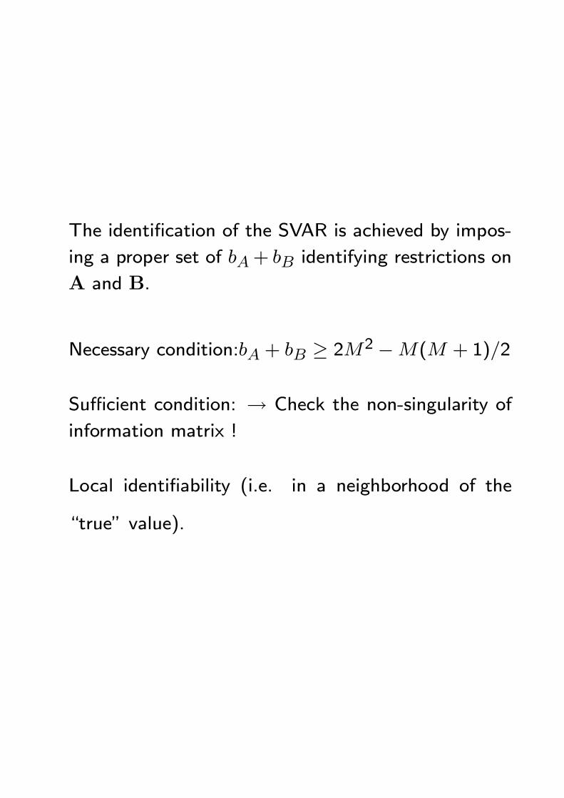
The identification of the SVAR is achieved by impos-

ing a proper set of bA+ bB identifying restrictions on

A and B.

Necessary condition:bA + bB ≥ 2M2 −M(M + 1)/2

Sufficient condition: → Check the non-singularity of

information matrix !

Local identifiability (i.e. in a neighborhood of the

“true” value).

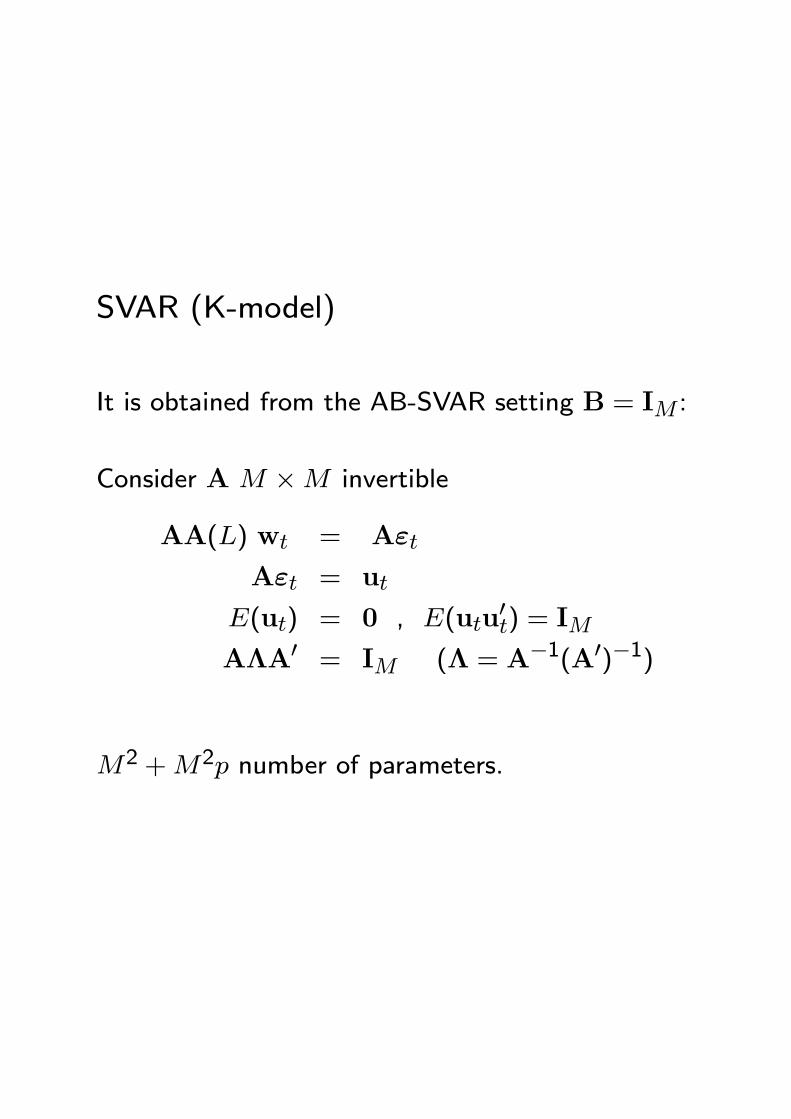
SVAR (K-model)

It is obtained from the AB-SVAR setting B = IM :

Consider A M ×M invertible

AA(L) wt = Aεt

Aεt = ut

E(ut) = 0 , E(utu0t) = IM

AΛA0 = IM (Λ = A−1(A0)−1)

M2 +M2p number of parameters.

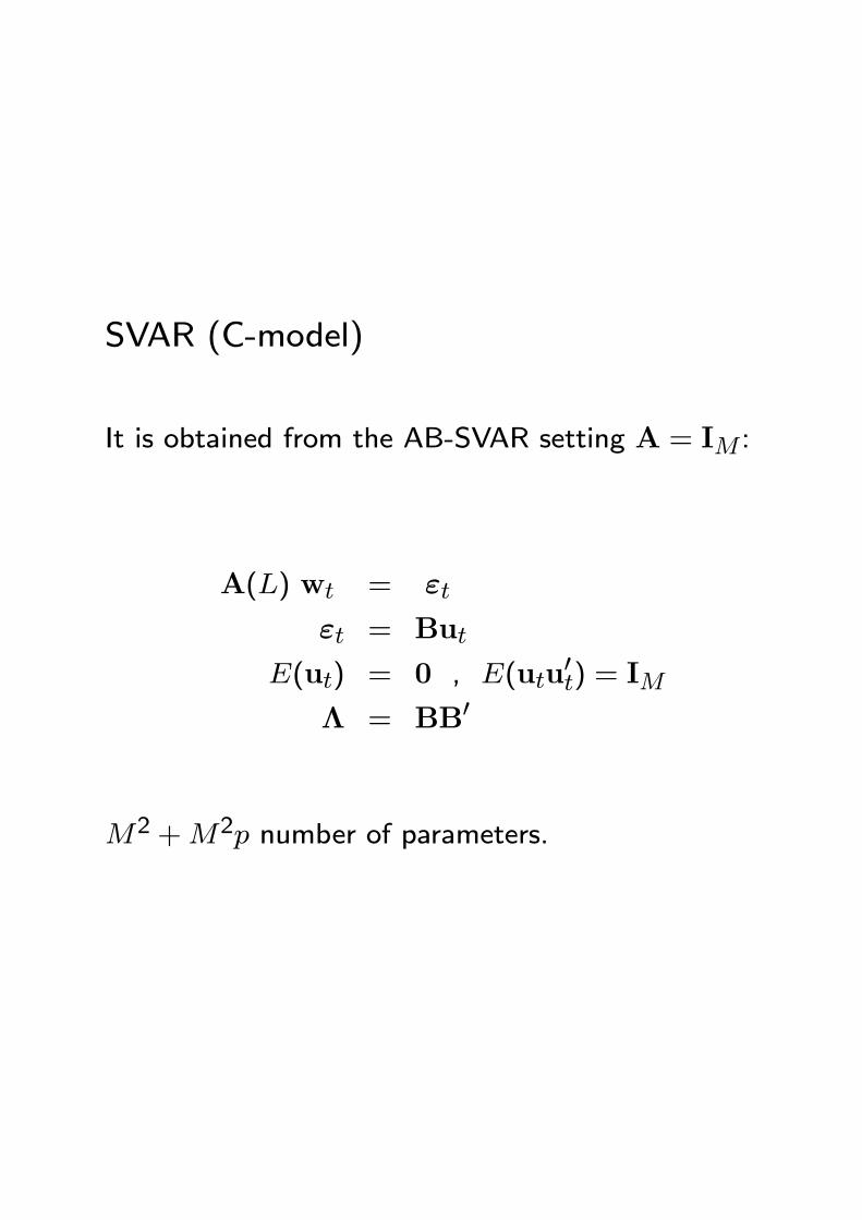
SVAR (C-model)

It is obtained from the AB-SVAR setting A = IM :

A(L) wt = εt

εt = But

E(ut) = 0 , E(utu0t) = IM

Λ = BB0

M2 +M2p number of parameters.

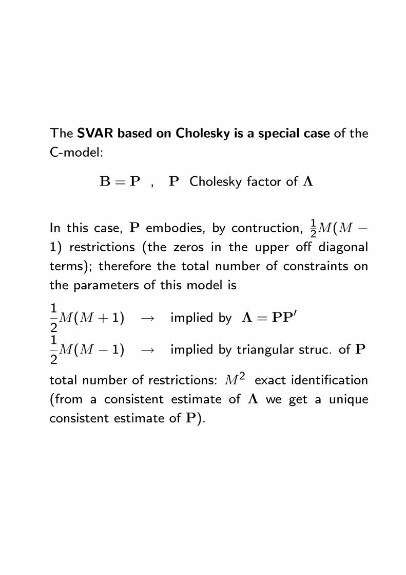
The SVAR based on Cholesky is a special case of the

C-model:

B = P , P Cholesky factor of Λ

In this case, P embodies, by contruction, 12M(M −1) restrictions (the zeros in the upper off diagonal

terms); therefore the total number of constraints on

the parameters of this model is

1

2M(M + 1) → implied by Λ = PP0

1

2M(M − 1) → implied by triangular struc. of P

total number of restrictions: M2 exact identification

(from a consistent estimate of Λ we get a unique

consistent estimate of P).

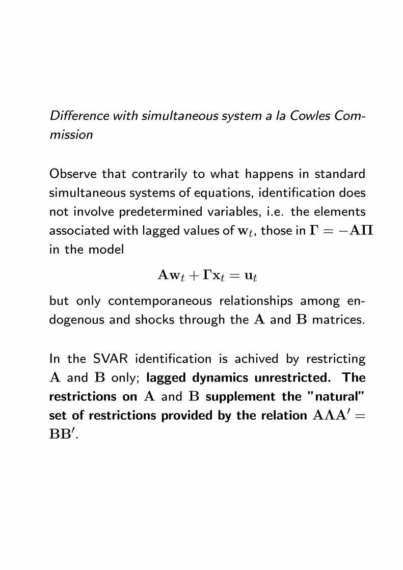
Difference with simultaneous system a la Cowles Com-

mission

Observe that contrarily to what happens in standard

simultaneous systems of equations, identification does

not involve predetermined variables, i.e. the elements

associated with lagged values ofwt, those in Γ = −AΠin the model

Awt + Γxt = ut

but only contemporaneous relationships among en-

dogenous and shocks through the A and B matrices.

In the SVAR identification is achived by restricting

A and B only; lagged dynamics unrestricted. The

restrictions on A and B supplement the ”natural”

set of restrictions provided by the relation AΛA0 =BB0.

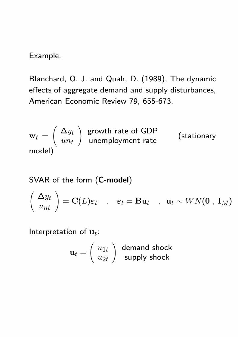
Example.

Blanchard, O. J. and Quah, D. (1989), The dynamic

effects of aggregate demand and supply disturbances,

American Economic Review 79, 655-673.

wt =

Ã∆ytunt

!growth rate of GDPunemployment rate

(stationary

model)

SVAR of the form (C-model)Ã∆ytunt

!= C(L)εt , εt = But , ut ∼WN(0 , IM)

Interpretation of ut:

ut =

Ãu1tu2t

!demand shocksupply shock

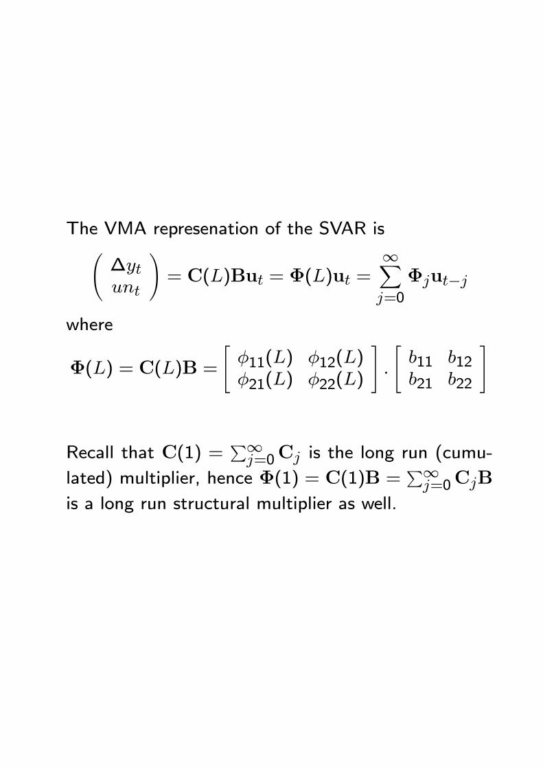
The VMA represenation of the SVAR isÃ∆ytunt

!= C(L)But = Φ(L)ut =

∞Xj=0

Φjut−j

where

Φ(L) = C(L)B =

"φ11(L) φ12(L)φ21(L) φ22(L)

#.

"b11 b12b21 b22

#

Recall that C(1) =P∞j=0Cj is the long run (cumu-

lated) multiplier, hence Φ(1) = C(1)B =P∞j=0CjB

is a long run structural multiplier as well.

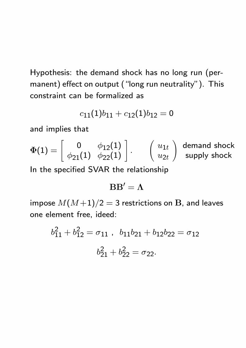
Hypothesis: the demand shock has no long run (per-

manent) effect on output (“long run neutrality”). This

constraint can be formalized as

c11(1)b11 + c12(1)b12 = 0

and implies that

Φ(1) =

"0 φ12(1)

φ21(1) φ22(1)

#.

Ãu1tu2t

!demand shocksupply shock

In the specified SVAR the relationship

BB0 = Λ

imposeM(M+1)/2 = 3 restrictions on B, and leaves

one element free, ideed:

b211 + b212 = σ11 , b11b21 + b12b22 = σ12

b221 + b222 = σ22.

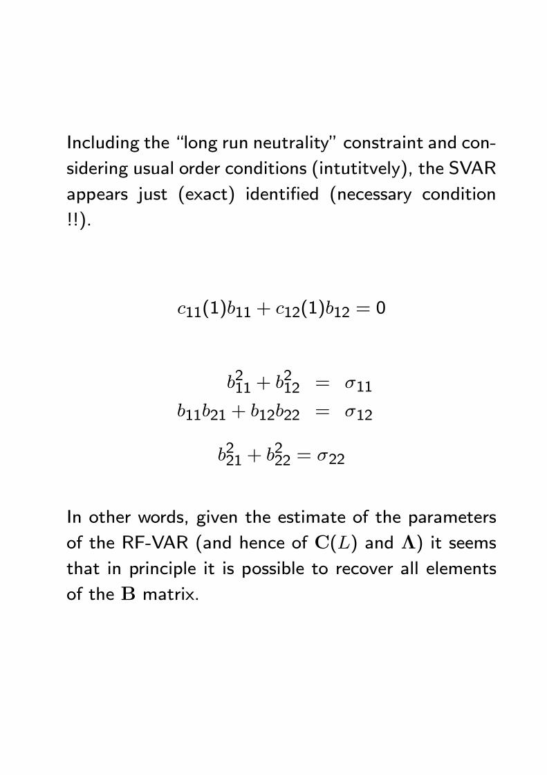
Including the “long run neutrality” constraint and con-

sidering usual order conditions (intutitvely), the SVAR

appears just (exact) identified (necessary condition

!!).

c11(1)b11 + c12(1)b12 = 0

b211 + b212 = σ11

b11b21 + b12b22 = σ12

b221 + b222 = σ22

In other words, given the estimate of the parameters

of the RF-VAR (and hence of C(L) and Λ) it seems

that in principle it is possible to recover all elements

of the B matrix.

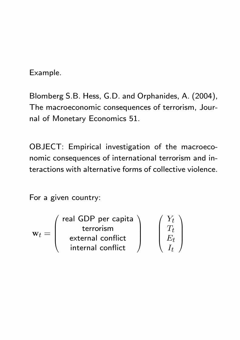
Example.

Blomberg S.B. Hess, G.D. and Orphanides, A. (2004),

The macroeconomic consequences of terrorism, Jour-

nal of Monetary Economics 51.

OBJECT: Empirical investigation of the macroeco-

nomic consequences of international terrorism and in-

teractions with alternative forms of collective violence.

For a given country:

wt =

real GDP per capita

terrorismexternal conflictinternal conflict

YtTtEtIt

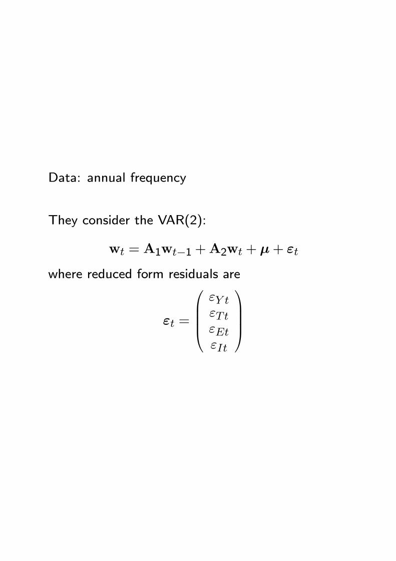
Data: annual frequency

They consider the VAR(2):

wt = A1wt−1 +A2wt + µ+ εt

where reduced form residuals are

εt =

εY tεTtεEtεIt

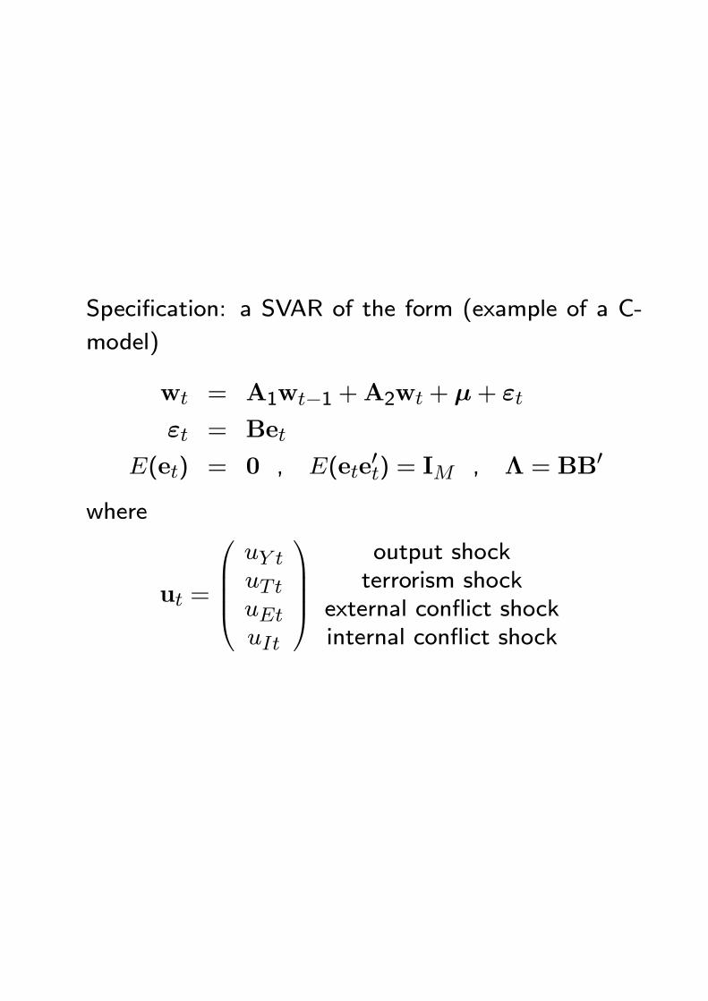
Specification: a SVAR of the form (example of a C-

model)

wt = A1wt−1 +A2wt + µ+ εt

εt = Bet

E(et) = 0 , E(ete0t) = IM , Λ = BB0

where

ut =

uY tuTtuEtuIt

output shockterrorism shock

external conflict shockinternal conflict shock

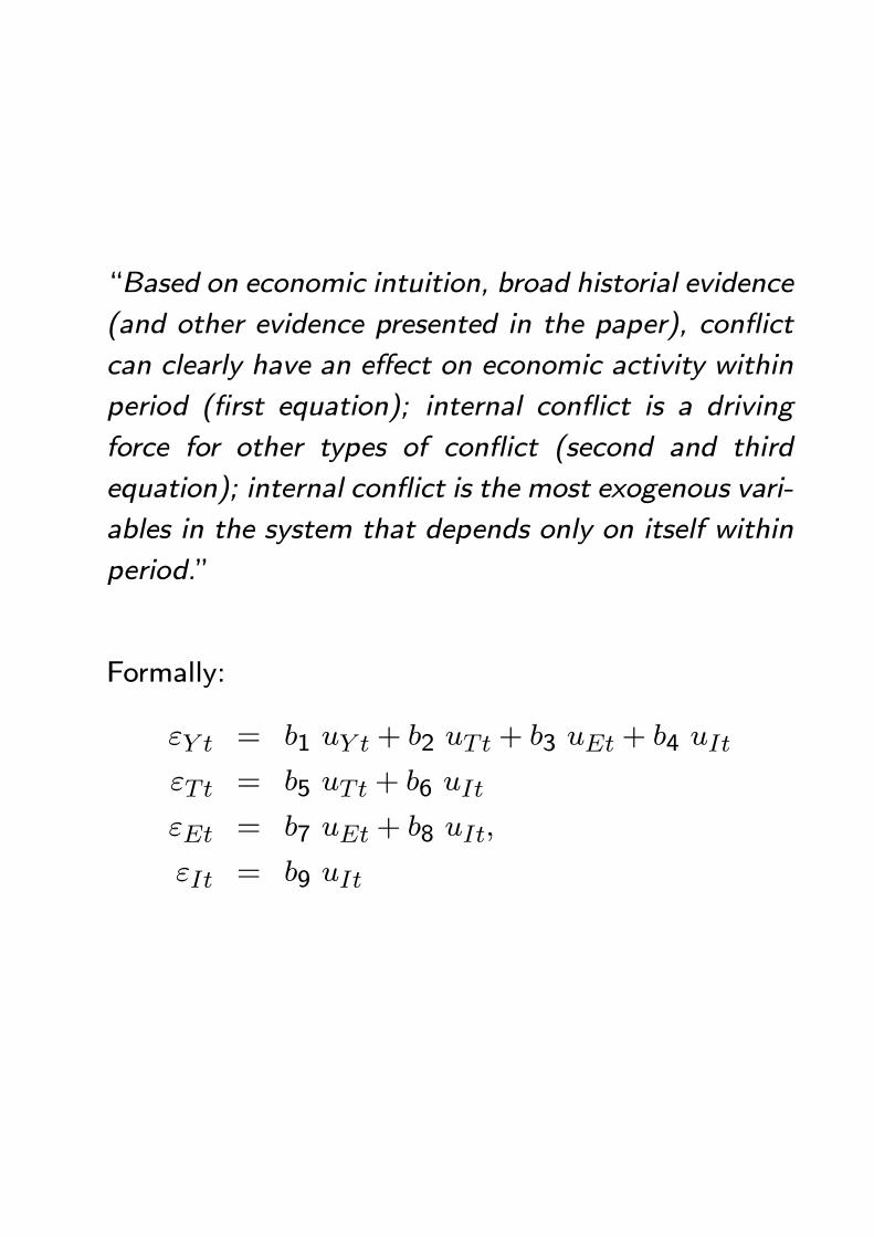
“Based on economic intuition, broad historial evidence

(and other evidence presented in the paper), conflict

can clearly have an effect on economic activity within

period (first equation); internal conflict is a driving

force for other types of conflict (second and third

equation); internal conflict is the most exogenous vari-

ables in the system that depends only on itself within

period.”

Formally:

εY t = b1 uY t + b2 uTt + b3 uEt + b4 uIt

εTt = b5 uTt + b6 uIt

εEt = b7 uEt + b8 uIt,

εIt = b9 uIt

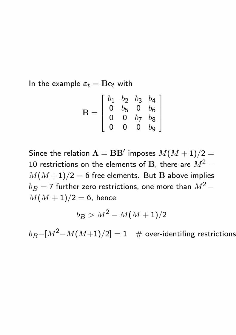
In the example εt = Bet with

B =

b1 b2 b3 b40 b5 0 b60 0 b7 b80 0 0 b9

Since the relation Λ = BB0 imposes M(M + 1)/2 =

10 restrictions on the elements of B, there are M2−M(M+1)/2 = 6 free elements. But B above implies

bB = 7 further zero restrictions, one more thanM2−

M(M + 1)/2 = 6, hence

bB > M2 −M(M + 1)/2

bB−[M2−M(M+1)/2] = 1 # over-identifing restrictions

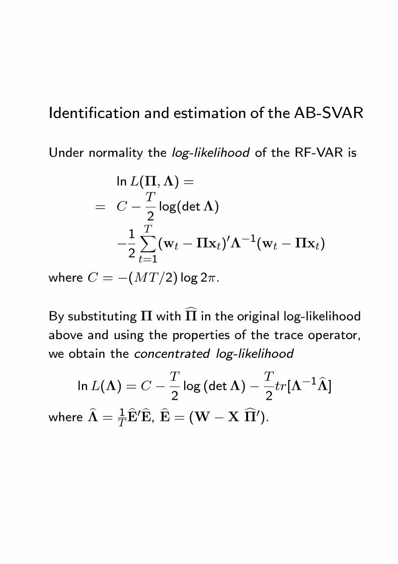
Identification and estimation of the AB-SVAR

Under normality the log-likelihood of the RF-VAR is

lnL(Π,Λ) =

= C − T

2log(detΛ)

−12

TXt=1

(wt −Πxt)0Λ−1(wt −Πxt)

where C = −(MT/2) log 2π.

By substitutingΠ with cΠ in the original log-likelihood

above and using the properties of the trace operator,

we obtain the concentrated log-likelihood

lnL(Λ) = C − T

2log (detΛ)− T

2tr[Λ−1 bΛ]

where bΛ = 1TbE0 bE, bE = (W−X cΠ0).

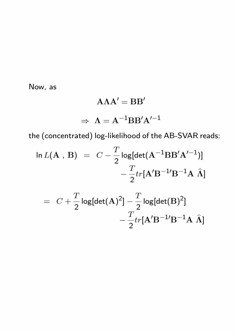
Now, as

AΛA0 = BB0

⇒ Λ = A−1BB0A0−1

the (concentrated) log-likelihood of the AB-SVAR reads:

lnL(A , B) = C − T

2log[det(A−1BB0A0−1)]

− T

2tr[A0B−10B−1A bΛ]

= C +T

2log[det(A)2]− T

2log[det(B)2]

− T

2tr[A0B−10B−1A bΛ]

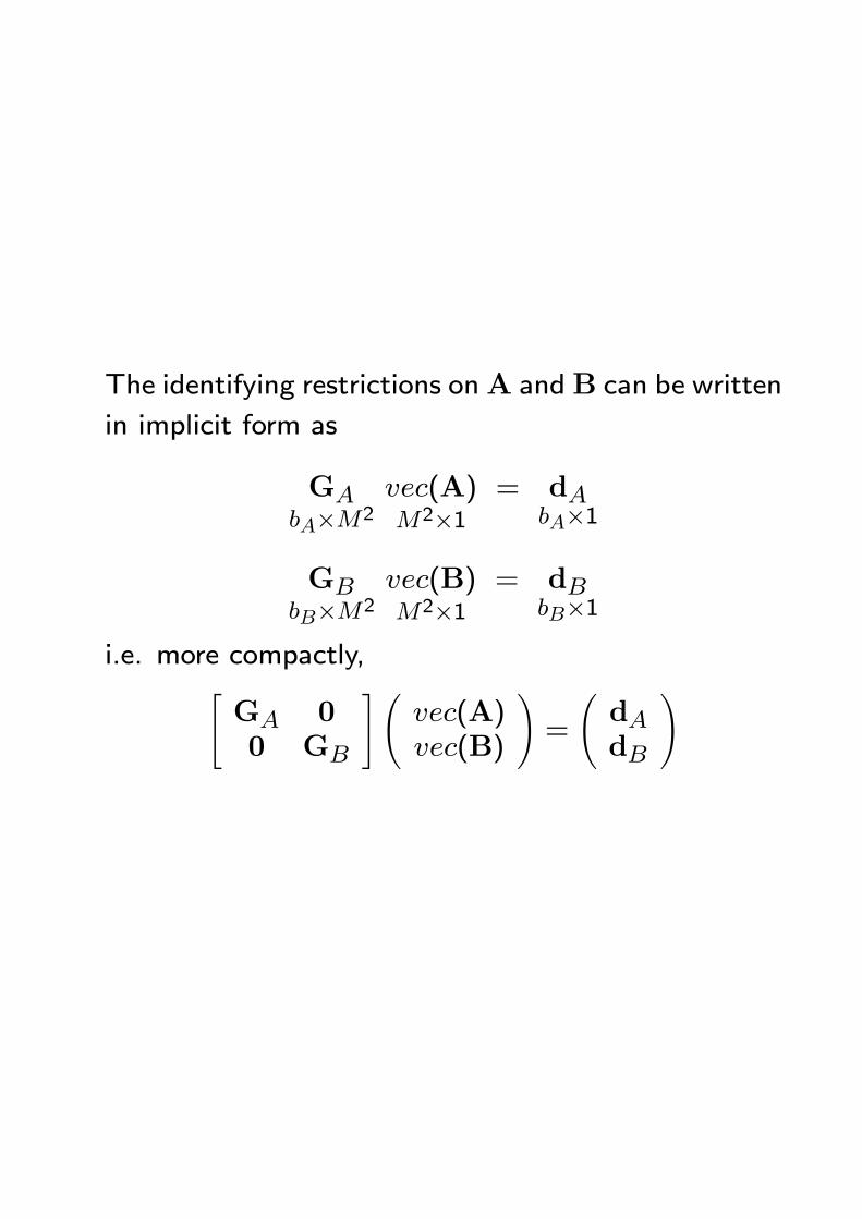
The identifying restrictions onA andB can be written

in implicit form as

GAbA×M2

vec(A)M2×1

= dAbA×1

GBbB×M2

vec(B)M2×1

= dBbB×1

i.e. more compactly,"GA 00 GB

#Ãvec(A)vec(B)

!=

ÃdAdB

!

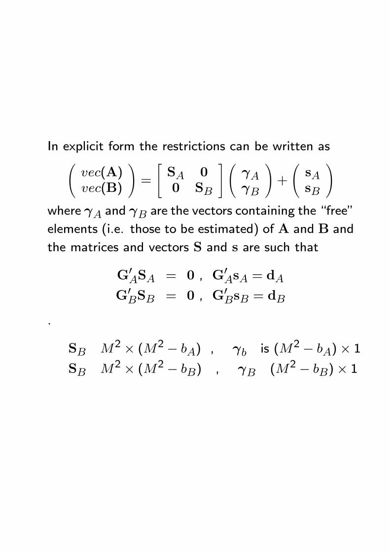
In explicit form the restrictions can be written asÃvec(A)vec(B)

!=

"SA 00 SB

#ÃγAγB

!+

ÃsAsB

!where γA and γB are the vectors containing the “free”

elements (i.e. those to be estimated) of A and B and

the matrices and vectors S and s are such that

G0ASA = 0 , G0AsA = dAG0BSB = 0 , G0BsB = dB

.

SB M2 × (M2 − bA) , γb is (M2 − bA)× 1SB M2 × (M2 − bB) , γB (M2 − bB)× 1

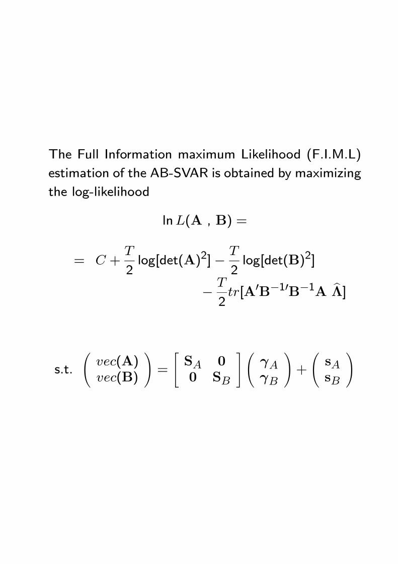
The Full Information maximum Likelihood (F.I.M.L)

estimation of the AB-SVAR is obtained by maximizing

the log-likelihood

lnL(A , B) =

= C +T

2log[det(A)2]− T

2log[det(B)2]

− T

2tr[A0B−10B−1A bΛ]

s.t.

Ãvec(A)vec(B)

!=

"SA 00 SB

#ÃγAγB

!+

ÃsAsB

!

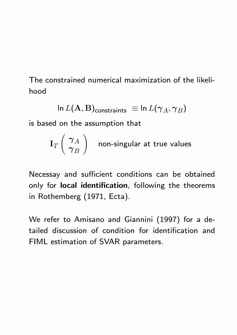
The constrained numerical maximization of the likeli-

hood

lnL(A,B)constraints ≡ lnL(γA,γB)is based on the assumption that

IT

ÃγAγB

!non-singular at true values

Necessay and sufficient conditions can be obtained

only for local identification, following the theorems

in Rothemberg (1971, Ecta).

We refer to Amisano and Giannini (1997) for a de-

tailed discussion of condition for identification and

FIML estimation of SVAR parameters.

As a rule, however, the Hessian and the sample In-

formation matrices are functions of the parameters

to be estimated, so they cannot be computed be-

fore estimation is carried out, rendering this type of

check non-operational → compute IT (·) at randompoints in the parameter space, Amisano and Giannini

(1997).

Lucchetti (2006, ET) has provided new conditions

(necessary and sufficient) for identification of SVARs

that do not involve γA and γB → algebra involved.

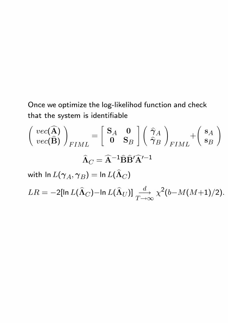
Once we optimize the log-likelihod function and check

that the system is identifiableÃvec(cA)vec( bB)

!FIML

=

"SA 00 SB

#Ã bγAbγB!FIML

+

ÃsAsB

!

bΛC =cA−1 bB bB0cA0−1

with lnL(γA,γB) = lnL(bΛC)

LR = −2[lnL( bΛC)−lnL( bΛU)]d−→

T→∞ χ2(b−M(M+1)/2).

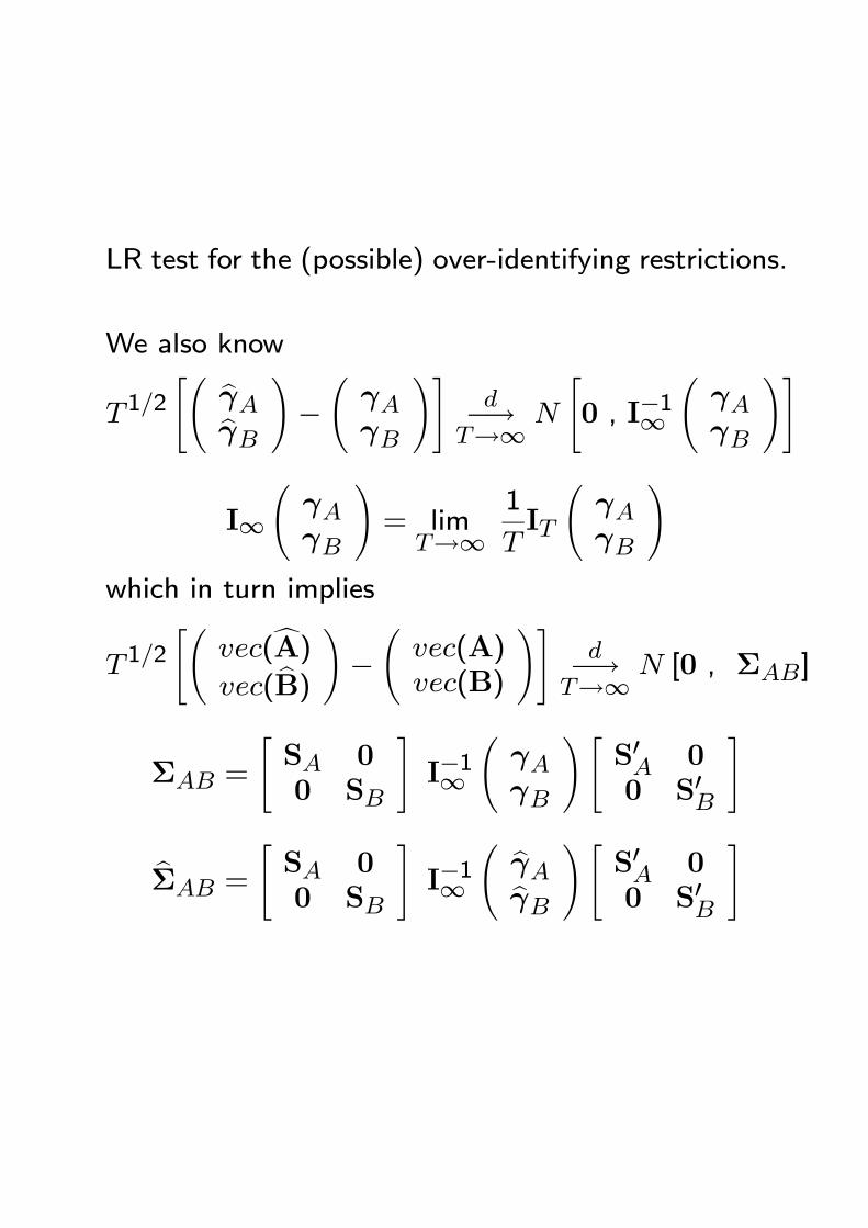
LR test for the (possible) over-identifying restrictions.

We also know

T 1/2"Ã bγAbγB

!−ÃγAγB

!#d−→

T→∞ N

"0 , I−1∞

ÃγAγB

!#

I∞ÃγAγB

!= lim

T→∞1

TIT

ÃγAγB

!which in turn implies

T 1/2"Ã

vec(cA)vec( bB)

!−Ãvec(A)vec(B)

!#d−→

T→∞ N [0 , ΣAB]

ΣAB =

"SA 00 SB

#I−1∞

ÃγAγB

!"S0A 00 S0B

#

bΣAB =

"SA 00 SB

#I−1∞

à bγAbγB!"

S0A 00 S0B

#

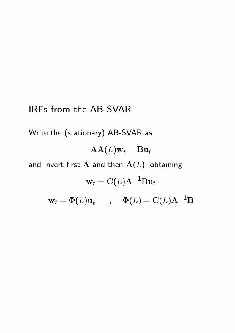
IRFs from the AB-SVAR

Write the (stationary) AB-SVAR as

AA(L)wt = But

and invert first A and then A(L), obtaining

wt = C(L)A−1But

wt = Φ(L)ut , Φ(L) = C(L)A−1B

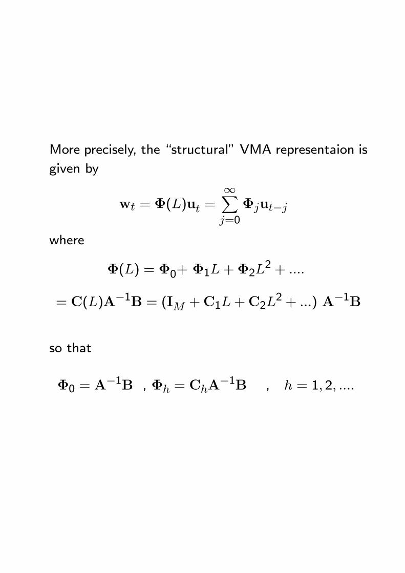
More precisely, the “structural” VMA representaion is

given by

wt = Φ(L)ut =∞Xj=0

Φjut−j

where

Φ(L) = Φ0+ Φ1L+Φ2L2 + ....

= C(L)A−1B = (IM +C1L+C2L2 + ...) A−1B

so that

Φ0 = A−1B , Φh = ChA

−1B , h = 1, 2, ....

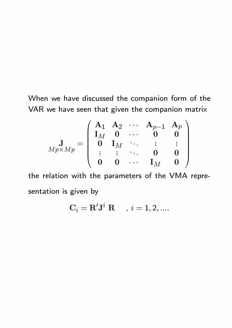
When we have discussed the companion form of the

VAR we have seen that given the companion matrix

JMp×Mp

=

A1 A2 · · · Ap−1 Ap

IM 0 · · · 0 00 IM

. . . ... ...... ... . . . 0 00 0 · · · IM 0

the relation with the parameters of the VMA repre-

sentation is given by

Ci = R0Ji R , i = 1, 2, ....

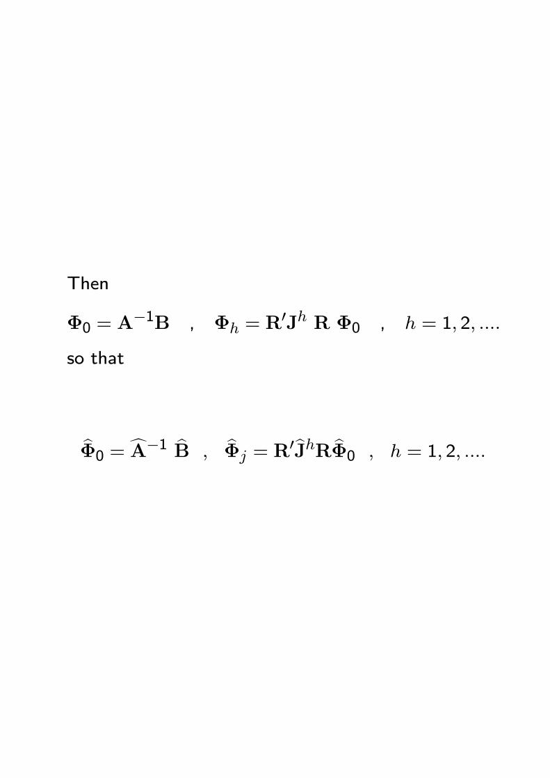
Then

Φ0 = A−1B , Φh = R

0Jh R Φ0 , h = 1, 2, ....

so that

bΦ0 = cA−1 bB , bΦj = R0bJhR bΦ0 , h = 1, 2, ....

Since cA , bB and cΠ (bJ) are consistent with Gaussianasymptotic distribution,

the bΦh, h = 0, 1, 2, .... will be consistent and asymp-

totically Gaussian as well.

It is possible to compute asymptotic confidence inter-

vals for impulse response functions.

Define the vector of structuralized impulses up to the

horizon n

φn = vec([Φ1 , Φ2 , ..., Φn]) , M2n× 1and

φ0 = vec(Φ0) , M2 × 1

φ0n = vec([Φ0, Φ1 , Φ2 , ..., Φn]) full M2(n+1)×1 vec

First, recall that

bΦ0 = cA−1 bBso that the asymptotic distribution of bφ0 will dependupon the joint distribution of vec(cA) and vec( bB) :tedious but feasible with a bit of patience, and using

matrix derivative rules.

It can be proved (Amisano, Giannini, 1997) that

T 1/2 (bφ0 − φ0)d−→

T→∞ N [0 , Σ(0)]

where Σ(0) depends on ΣAB, A and B, and can

be estimated consistently by replacing A and B in

the expression for Σ(0) with their consistent estimatesbΣAB,cA and bB.

Likewise:

T 1/2 (bφn − φn)d−→

T→∞ N [0 , Σ(n)]

where the ij-th block of Σ(n) (which isM2n×M2n),

Σ(n)ij, is M2×M2 and depends opportunely on the

elements of the companion matrix J and Φ0, and can

be estimated opportunely by replacing J andΦ0 in the

expression for Σ(n)ij with their consistent estimatesbJ and bΦ0.Observe that the Σ(n)ii block of Σ(n), i = 1, 2, ..., n

corresponds to the variance covariance matrix of vec(Φi).

Knowledge of bφ0n = vec([ bΦ0 , bΦ1 , bΦ2 , ..., bΦn])

(vector of structuralized impulse responses) and the

associated joint (estimated) covariance matrix allows

to calculate asymptotic confidence intervals for im-

pulse responses.