The E ects of Realistic Geological Heterogeneity on ... · The E ects of Realistic Geological Heterogeneity on Seismic Modeling: Applications in Shear Wave Generation and Near-Surface

The Effects of Realistic Geological Heterogeneity on Seismic Modeling:Applications in Shear Wave Generation and Near-Surface Tunnel Detection

by

Christopher Scott Sherman

A dissertation submitted in partial satisfaction of the

requirements for the degree of

Doctor of Philosophy

in

Engineering - Civil and Environmental Engineering

in the

Graduate Division

of the

University of California, Berkeley

Committee in charge:

Professor Steven D. Glaser, ChairProfessor James W. RectorProfessor Douglas Dreger

Fall 2014

The Effects of Realistic Geological Heterogeneity on Seismic Modeling:Applications in Shear Wave Generation and Near-Surface Tunnel Detection

Copyright 2014by


1

Abstract

The Effects of Realistic Geological Heterogeneity on Seismic Modeling: Applications inShear Wave Generation and Near-Surface Tunnel Detection

by


Doctor of Philosophy in Engineering - Civil and Environmental Engineering

University of California, Berkeley

Professor Steven D. Glaser, Chair

Naturally occurring geologic heterogeneity is an important, but often overlooked, aspectof seismic wave propagation. This dissertation presents a strategy for modeling the effectsof heterogeneity using a combination of geostatistics and Finite Difference simulation.

In the first chapter, I discuss my motivations for studying geologic heterogeneity and seis-mic wave propagation. Models based upon fractal statistics are powerful tools in geophysicsfor modeling heterogeneity. The important features of these fractal models are illustratedusing borehole log data from an oil well and geomorphological observations from a site inDeath Valley, California. A large part of the computational work presented in this disserta-tion was completed using the Finite Difference Code E3D. I discuss the Python-based userinterface for E3D and the computational strategies for working with heterogeneous modelsdeveloped over the course of this research.

The second chapter explores a phenomenon observed for wave propagation in heteroge-neous media - the generation of unexpected shear wave phases in the near-source region.In spite of their popularity amongst seismic researchers, approximate methods for modelingwave propagation in these media, such as the Born and Rytov methods or Radiative Trans-fer Theory, are incapable of explaining these shear waves. This is primarily due to thesemethod’s assumptions regarding the coupling of near-source terms with the heterogeneitiesand mode conversion. To determine the source of these shear waves, I generate a suite of 3Dsynthetic heterogeneous fractal geologic models and use E3D to simulate the wave propaga-tion for a vertical point force on the surface of the models. I also present a methodology forcalculating the effective source radiation patterns from the models. The numerical resultsshow that, due to a combination of mode conversion and coupling with near-source hetero-geneity, shear wave energy on the order of 10 % of the compressional wave energy may begenerated within the shear radiation node of the source. Interestingly, in some cases thisshear wave may arise as a coherent pulse, which may be used to improve seismic imagingefforts.

2

In the third and fourth chapters, I discuss the results of a numerical analysis and fieldstudy of seismic near-surface tunnel detection methods. Detecting unknown tunnels andvoids, such as old mine workings or solution cavities in karst terrain, is a challenging prob-lem in geophysics and has implications for geotechnical design, public safety, and domesticsecurity. Over the years, a number of different geophysical methods have been developedto locate these objects (microgravity, resistivity, seismic diffraction, etc.), each with varyingresults. One of the major challenges facing these methods is understanding the influence ofgeologic heterogeneity on their results, which makes this problem a natural extension of themodeling work discussed in previous chapters. In the third chapter, I present the results of anumerical study of surface-wave based tunnel detection methods. The results of this analysisshow that these methods are capable of detecting a void buried within one wavelength of thesurface, with size potentially much less than one wavelength. In addition, seismic surface-wave based detection methods are effective in media with moderate heterogeneity (ε < 5 %),and in fact, this heterogeneity may serve to increase the resolution of these methods. In thefourth chapter, I discuss the results of a field study of tunnel detection methods at a sitewithin the Black Diamond Mines Regional Preserve, near Antioch California. I use a com-bination of surface wave backscattering, 1D surface wave attenuation, and 2D attenuationtomography to locate and determine the condition of two tunnels at this site. These resultscompliment the numerical study in chapter 3 and highlight their usefulness for detectingtunnels at other sites.

i

To my mother, whose endless support has made this possible.

ii

Contents

Contents ii

List of Figures iv

1 Overview 11.1 Introduction . . . . . . . . . . . . . . . . . . . . . . . . . . . . . . . . . . . . 11.2 Geologic Heterogeneity . . . . . . . . . . . . . . . . . . . . . . . . . . . . . . 11.3 Numerical Simulations and Heterogeneity . . . . . . . . . . . . . . . . . . . . 71.4 PyE3D . . . . . . . . . . . . . . . . . . . . . . . . . . . . . . . . . . . . . . . 81.5 Case Studies . . . . . . . . . . . . . . . . . . . . . . . . . . . . . . . . . . . . 8

2 Near Source Heterogeneity 102.1 Introduction . . . . . . . . . . . . . . . . . . . . . . . . . . . . . . . . . . . . 102.2 Model of Geologic Heterogeneity . . . . . . . . . . . . . . . . . . . . . . . . . 122.3 Numerical Analysis . . . . . . . . . . . . . . . . . . . . . . . . . . . . . . . . 142.4 Effective Source Radiation Patterns . . . . . . . . . . . . . . . . . . . . . . . 152.5 Results . . . . . . . . . . . . . . . . . . . . . . . . . . . . . . . . . . . . . . . 17

2.5.1 Homogeneous velocity model . . . . . . . . . . . . . . . . . . . . . . . 172.5.2 Isotropic fractal velocity models . . . . . . . . . . . . . . . . . . . . . 182.5.3 Layered fractal velocity models . . . . . . . . . . . . . . . . . . . . . 212.5.4 Reflecting velocity models . . . . . . . . . . . . . . . . . . . . . . . . 24

2.6 Discussion . . . . . . . . . . . . . . . . . . . . . . . . . . . . . . . . . . . . . 252.7 Conclusion . . . . . . . . . . . . . . . . . . . . . . . . . . . . . . . . . . . . . 27

3 Modeling Tunnel Detection 293.1 Introduction . . . . . . . . . . . . . . . . . . . . . . . . . . . . . . . . . . . . 293.2 Background on Void Detection Methods . . . . . . . . . . . . . . . . . . . . 293.3 Surface Wave Methods and Geological Heterogeneity . . . . . . . . . . . . . 313.4 Case Study: Black Diamond Mines . . . . . . . . . . . . . . . . . . . . . . . 313.5 Modeling Geologic Heterogeneity . . . . . . . . . . . . . . . . . . . . . . . . 323.6 Numerical Analysis . . . . . . . . . . . . . . . . . . . . . . . . . . . . . . . . 323.7 Theory . . . . . . . . . . . . . . . . . . . . . . . . . . . . . . . . . . . . . . . 34

iii

3.7.1 Surface Wave Backscattering . . . . . . . . . . . . . . . . . . . . . . . 343.7.2 Surface Wave Attenuation . . . . . . . . . . . . . . . . . . . . . . . . 343.7.3 Effect of Void Size and Depth . . . . . . . . . . . . . . . . . . . . . . 35

3.8 Results . . . . . . . . . . . . . . . . . . . . . . . . . . . . . . . . . . . . . . . 363.8.1 Homogeneous Background Model . . . . . . . . . . . . . . . . . . . . 363.8.2 Heterogeneous Background Model . . . . . . . . . . . . . . . . . . . . 383.8.3 Effect of Void Depth and Location . . . . . . . . . . . . . . . . . . . 403.8.4 Effect of Heterogeneity . . . . . . . . . . . . . . . . . . . . . . . . . . 433.8.5 Effect of Array Geometry . . . . . . . . . . . . . . . . . . . . . . . . 43

3.9 Discussion . . . . . . . . . . . . . . . . . . . . . . . . . . . . . . . . . . . . . 463.10 Conclusion . . . . . . . . . . . . . . . . . . . . . . . . . . . . . . . . . . . . . 46

4 Tunnel Detection at BDM 474.1 Introduction . . . . . . . . . . . . . . . . . . . . . . . . . . . . . . . . . . . . 474.2 Description of Field Study . . . . . . . . . . . . . . . . . . . . . . . . . . . . 48

4.2.1 Black Diamond Mines Regional Preserve . . . . . . . . . . . . . . . . 484.2.2 Instrumentation . . . . . . . . . . . . . . . . . . . . . . . . . . . . . . 49

4.3 Theory / Processing . . . . . . . . . . . . . . . . . . . . . . . . . . . . . . . 514.3.1 Surface Wave Backscattering . . . . . . . . . . . . . . . . . . . . . . . 514.3.2 1D Surface Wave Attenuation . . . . . . . . . . . . . . . . . . . . . . 524.3.3 2D Surface Wave Attenuation Tomography . . . . . . . . . . . . . . . 524.3.4 Microgravity . . . . . . . . . . . . . . . . . . . . . . . . . . . . . . . . 53

4.4 Results . . . . . . . . . . . . . . . . . . . . . . . . . . . . . . . . . . . . . . . 544.5 Discussion . . . . . . . . . . . . . . . . . . . . . . . . . . . . . . . . . . . . . 574.6 Conclusion . . . . . . . . . . . . . . . . . . . . . . . . . . . . . . . . . . . . . 59

5 Conclusion 605.1 Modeling Geological Heterogeneity . . . . . . . . . . . . . . . . . . . . . . . 60

5.1.1 Shear Wave Generation . . . . . . . . . . . . . . . . . . . . . . . . . . 615.1.2 Near Surface Tunnel Detection . . . . . . . . . . . . . . . . . . . . . 61

5.2 Future Work . . . . . . . . . . . . . . . . . . . . . . . . . . . . . . . . . . . . 61

A PyE3D Manual 62

Bibliography 76

iv

List of Figures

1.1 Typical data collected for an (a) sonic log and (b) resistivity log for an oil well. . 31.2 Fourier Transform of the (a) sonic log and (b) resistivity log data shown in Figures

?? and ??. . . . . . . . . . . . . . . . . . . . . . . . . . . . . . . . . . . . . . . . 41.3 Salt crystal as seen from the floor of Death Valley, California. . . . . . . . . . . 51.4 Examples of synthetic isotropic fractal models for β = (a) 1.0, (b) 1.2, (c) 1.4,

(d) 1.6, . . . . . . . . . . . . . . . . . . . . . . . . . . . . . . . . . . . . . . . . 61.5 Examples of synthetic isotropic fractal models for β = 1.4 and az = (a) 1.0, (b)

0.5, (c) 0.25, (d) 0.125, . . . . . . . . . . . . . . . . . . . . . . . . . . . . . . . . 7

2.1 Cross-section through a synthetic fractal velocity model with VP = 3 km/s, ε =1 %, and β = 1.7. The heterogeneity is confined to the upper third of the model. 13

2.2 Model geometry for the finite difference simulations. . . . . . . . . . . . . . . . . 152.3 (left) Comparison of the effective radiation patterns, Rs

eff and Rpeff , for the ho-

mogeneous reference model (black) and the closed-form solution (red). (right)Close up view of the shear radiation patterns. . . . . . . . . . . . . . . . . . . . 18

2.4 (left) Comparison of the effective radiation patterns, Rseff and Rp

eff , for anisotropic heterogeneous model with β = 1.7, ε = 1.5 %, and r = 5λo (black),and the homogeneous reference model (red). (right) Close up view of the shearradiation patterns. . . . . . . . . . . . . . . . . . . . . . . . . . . . . . . . . . . 19

2.5 The Rseff/R

peff for an isotropic fractal model throughout the domain (β = 1.7

and ε = 1.5 %). . . . . . . . . . . . . . . . . . . . . . . . . . . . . . . . . . . . . 192.6 Horizontal wavefield directly beneath the point source for an isotropic fractal

model (β = 1.7 and ε = 1.5 %). . . . . . . . . . . . . . . . . . . . . . . . . . . . 202.7 (a) Effect of fractal amplitude (ε) on Rs

eff/Rpeff beneath the source. (b)Effect of

fractal dimension (β) on Rseff/R

peff beneath the source. . . . . . . . . . . . . . . 22

2.8 (left) Comparison of the effective radiation patterns, Rseff and Rp

eff , for a layeredfractal model with ε = 1.6 %, β = 1.7, and b = 10 (black), and the homogeneousreference model (red). (right) Close up view of the shear radiation patterns. . . 23

2.9 Horizontal wavefield directly beneath the point source for a layered fractal model(ε = 1.6 %, β = 1.7, and b = 10). . . . . . . . . . . . . . . . . . . . . . . . . . . 23

2.10 Effect of fractal amplitude (ε) on Rseff/R

peff for a layered fractal model directly

beneath the source. . . . . . . . . . . . . . . . . . . . . . . . . . . . . . . . . . . 24

v

2.11 Horizontal wavefield directly beneath the point force for a reflecting fractal model. 252.12 Correlations of ε and Rs

eff/Rpeff for the isotropic fractal models (R2 = 0.98) and

layered fractal models (R2 = 0.99). . . . . . . . . . . . . . . . . . . . . . . . . . 26

3.1 Block diagram showing numerical model geometry and a single realization of thefractal heterogeneity (β = 1.7, ε = 2 %). . . . . . . . . . . . . . . . . . . . . . . 33

3.2 (a) Measured Vz along the top of the model for a homogeneous background mate-rial. (b) Measured Vz along the top of the model for a homogeneous backgroundmaterial after applying AGC and the directional f-k filter. . . . . . . . . . . . . 37

3.3 Surface wave attenuation curve for a model with a homogenous background ma-terial. . . . . . . . . . . . . . . . . . . . . . . . . . . . . . . . . . . . . . . . . . 38

3.4 (a) Measured Vz along the top of the model for a heterogeneous backgroundmaterial (β = 1.7, ε = 2 %). (b) Measured Vz along the top of the model for theheterogeneous background material after applying AGC and the directional f-kfilter. . . . . . . . . . . . . . . . . . . . . . . . . . . . . . . . . . . . . . . . . . . 39

3.5 Surface wave attenuation curve for a model with a heterogeneous backgroundmaterial with (solid) and without (dotted) the buried tunnel. . . . . . . . . . . . 40

3.6 Effect of tunnel depth on surface wave attenuation curve for a mean frequency of(a) 100Hz, (b) 150Hz. . . . . . . . . . . . . . . . . . . . . . . . . . . . . . . . 41

3.7 (a) Effect of tunnel depth on surface wave attenuation curve for a mean frequencyof 200Hz. (b) The maximum deviation from the predicted attenuation curve forscaled depth. . . . . . . . . . . . . . . . . . . . . . . . . . . . . . . . . . . . . . 42

3.8 (a) Surface wave attenuation curves for models with heterogeneity amplitude, ε,ranging from 0.5 − 4 %. (b) Mean surface wave attenuation curves for differentvalues of ε. . . . . . . . . . . . . . . . . . . . . . . . . . . . . . . . . . . . . . . 44

3.9 Surface wave attenuation curves measured at different angles from the tunnel axisfor an (a) homogeneous background model, (b) heterogeneous background model. 45

4.1 The experimental site (BDM) is located within the Black Diamond Mines Re-gional Preserve, near Antioch, California, USA. . . . . . . . . . . . . . . . . . . 49

4.2 (a) A plan view representation of the experimental site, which shows the locationof the linear seismic array (L-Array), rectangular seismic array (R-Array), theupper tunnel (UT), and the lower tunnel (LT). The location of the upper tunnelis known from historical survey data, and the exact location of the lower tunnelis unknown. (b) A cross-section view of the site, which shows the approximatelocations of the upper and lower tunnels, the subsidence pit that opened in 1998,and the proposed location of the stoping failure associated with the pit. . . . . . 50

vi

4.3 (a) An example of the seismic data collected using the L-Array, with the sourceoffset 15.2m to the north of the array. These data have been corrected for ge-ometric spreading and are for the frequency range of 2.5 to 10Hz. [The southend of the array corresponds to a distance of 0m.] (b) Seismic records from theL-Array that have been processed to emphasize surface wave backscattering. Theprimary backscattered waves are highlighted in red, and the resonant emissionsare highlighted in blue. The two apparent sources of these waves are located ata distance of 40 and 58m from the south end of the array. . . . . . . . . . . . . 54

4.4 (a) The measured surface wave attenuation curve for the L-Array. There aresignificant deviations from the average trend at a distance of about 35m and65m from the south of the L-Array. (b) A plot of the limited microgravity dataversus distance from the south side of the L-Array. There is an anomaly of about0.15mGal near the expected location of the upper tunnel (Distance ≈ 22m). . . 55

4.5 The inverted values of Q from the 2D surface wave attenuation analysis (thesouthwest corner of the R-Array is located at [0, 0]m). There are two discreteregions of low-Q observed within the array. . . . . . . . . . . . . . . . . . . . . . 56

4.6 A schematic showing the locations of the low-Q regions observed in the 1D and2D surface wave attenuation analyses, the location of the backscatterers (B0 andB1) observed in the surface wave backscattering analysis, and the low densityregion observed in the microgravity analysis. My estimates of the location of theupper and lower tunnels are indicated. . . . . . . . . . . . . . . . . . . . . . . . 58

A.1 PyE3D GUI Main Tab . . . . . . . . . . . . . . . . . . . . . . . . . . . . . . . . 65A.2 PyE3D GUI Advanced Tab . . . . . . . . . . . . . . . . . . . . . . . . . . . . . 67A.3 PyE3D GUI Materials Tab . . . . . . . . . . . . . . . . . . . . . . . . . . . . . . 69A.4 PyE3D GUI Sources Tab . . . . . . . . . . . . . . . . . . . . . . . . . . . . . . . 71A.5 PyE3D GUI Traces Tab . . . . . . . . . . . . . . . . . . . . . . . . . . . . . . . 72A.6 PyE3D GUI Movies Tab . . . . . . . . . . . . . . . . . . . . . . . . . . . . . . . 73A.7 PyE3D GUI Rerendering Tab . . . . . . . . . . . . . . . . . . . . . . . . . . . . 74

vii

Acknowledgments

I first became interested in seismic wave propagation in heterogeneous media during acourse on advanced seismology taught by Professor Jamie Rector at the University of Cali-fornia Berkeley. The question I asked myself was that, using a simple model for heterogeneityin a numerical simulation, is it possible to generate “realistic”-looking waveforms? Wouldseismic coda wave arise from such a model? How would these relate to “reai-world” geo-logic systems and measurements? To tackle these questions, I was introduced to the FiniteDifference wave propagation code E3D, which is developed at Lawrence Livermore NationalLaboratory by Shawn Larson. With this as my starting point, I have explored the problemof generating synthetic heterogeneous geological models, the numerical aspects of modelingwave propagation in heterogeneous media, and have been fortunate to have a number of casestudies to work from.

In particular, I would like to thank my co-advisers at UC Berkeley: Steve Glaser andJamie Rector. I am grateful for the freedom they gave me to explore all of the diverse topicsof interest to me in my research, and for their encouragement to work on a variety of (andoften completely unrelated) side-projects and collaborations with other researchers.

I would like to thank my lab-mates at Berkeley for their support: Paul Selvadurai, MarioMagliocco, Greg McLaskey, Branko Kerkez, and Ziran Zhang. Their friendship and willing-ness to engage in countless hours of debate and discussion have helped me tremendously.

I would also like to give special thanks to Doug Dreger from the Berkeley SeismologicalLaboratory whom I have taught alongside, has given many hours of advice, served as acommittee member, and has taught me a great deal about seismology.

Finally, I would like to thank my close friends and family for all of their support duringmy time at UC Berkeley.

1

Chapter 1

Overview

1.1 Introduction

One of the most common assumptions applied in classical physics is that, at some criticalscale, the object of interest is homogeneous. This critical step permits us to arrive at ele-gant and powerful relationships that describe natural phenomena and to perform useful andtimely work in science and engineering. The major drawback here is that, by ignoring hetero-geneity, one steps back from the wonderful complexity of nature and smooth out informationthat could help solve problems. For problems involving seismic wave propagation throughnaturally occurring geologic materials, the assumption of homogeneity is especially criti-cal: Countless observations have shown that the earth is heterogeneous over scales rangingfrom the microscopic to the size of entire geologic formations and that these heterogeneitiescontribute to phenomena such as coda wave generation, attenuation, etc.

1.2 Geologic Heterogeneity

A convenient starting point for discussing heterogeneity in the earth is the down-hole geo-physical log. These are common tools used in the geological exploration industry for measur-ing different properties of materials such as seismic velocity, electrical resistivity, or density.An example of a typical sonic log, which measures Vp, and resistivity log for an oil well areincluded in Figures 5.1 and 1.1b. To the first order, the material in this interval could bedescribed by an average seismic velocity (Vp ≈ 3.5 km/s) and resistivity (ρ ≈ 5 Ωm), and toa second order could be described by an average velocity and resistivity that changes withdepth.

In order to characterize the heterogeneity in a borehole log, it is necessary to remove theaverage values or trends from the log. The remaining data is considered to be with depth,which may be evaluated using signal processing techniques. A log-log frequency domainplot of the detrended sonic and resistivity logs from before is shown in Figures 1.2a and1.2b. Of particular note is that in the frequency domain, the shape of these two signals is

CHAPTER 1. OVERVIEW 2

very similar. Up to some corner value of wavenumber (here, Kz ≈ 1m−1) the curves areapproximately linear, and afterwards they drop off. From geostatistics, common optionsfor fitting these curves in the frequency domain include the Gaussian, exponential, and vonKarman functions (Sato, Fehler, and Maeda 2012). In this research, I consider the linearportion of the curves to be of the form given by Equation 1.1 (an exponential curve) andconsider the remaining signal to be instrument noise.

log(A) = (−β/2) · log(Kz) + A∗ (1.1)

Here A is the amplitude, Kz is the vertical wavenumber, A∗ is the intercept value, andβ is the fractal exponent. In simple terms, β controls the degree of correlation betweenindividual regions in a material, and A∗ controls the amplitude of heterogeneity. A majorbenefit of this type of model is that it displays a feature common to many geologic systems:scale invariance. To illustrate this feature, I have included a photograph of salt crystalstaken on the floor of Death Valley, California in Figure 1.3. The surface of the single crystalin the foreground has a particular jagged topography. Looking at the next row of saltcrystals in the image, and moving from a scale of millimeters to meters, there appears to bea very similar level of topography. What is remarkable is that this same topography of themountain range in the background, which is on the scale of kilometers, displays the sametype of topography. What this means for a scale invariant system, is that if you take animage of some feature, measure its topography, seismic velocity, resistivity, etc., it wouldbe impossible to determine the scale of the image without some external reference. In asimilar manner, a synthetic model that displays scale invariance may be used to simulatethe behavior of a system regardless of scale.


2 3 4 5 6 7

300

400

500

600

700

800

VP (km/s)

Dep

th (

m)

(a)

0 20 40 60 80 100

300

400

500

600

700

800

Dep

th (

m)

Resistivity (Ω m)

(b)

Figure 1.1: Typical data collected for an (a) sonic log and (b) resistivity log for an oil well.


10-2

10-1

100

10-3

10-2

10-1

100

Kz (1/m)

Am

plit

ud

e

(a)

10-2

10-1

100

10-3

10-2

10-1

100

Kz (1/m)

Am

plit

ud

e

(b)

Figure 1.2: Fourier Transform of the (a) sonic log and (b) resistivity log data shown inFigures 5.1 and 1.1b.


Figure 1.3: Salt crystal as seen from the floor of Death Valley, California.

In order for this exponential fractal model to be of use in numerical simulations, it isnecessary to create an arbitrary number of synthetic realizations of the model. To do this,I begin by considering an n-dimensional matrix of random, normal, independent numbers(white noise): G[x]. Next, I compute the Fourier transform of the matrix to arrive at G∗[k],which is a matrix of white noise with the same amplitude and variance as G[x]. To imposethe fractal model on this matrix, I multiply G∗ by the fractal filter given in 1.2 in thefrequency domain.

S = |k|−β/2 (1.2)

Here, S is a version of Equation 1.1 that has the intercept term removed and is generalizedto n-dimensions. The inverse Fourier transform is applied to the results, and the imaginarycomponent is discarded. As a result of not including an intercept factor in Equation 1.2,it is necessary to scale the results to have the appropriate standard deviation, which maybe estimated in the spatial domain for the target. Finally, to arrive at a synthetic fractalmodel, it is necessary to add the desired mean value and/or trends to the results.

Four examples of a synthetic fractal models for different values of β are included in Figures1.4a to 1.4d. These show the degree of variability that may be achieved by modifying thefractal dimension. In general, as β becomes larger, the model becomes more smooth. Notethat, while it is preferable to estimate β directly from observations such as the sonic log inFigure 5.1, it is possible to arrive at an estimate of β by considering information such as thedepositional environment (Browaeys and Fomel 2009).

While this type of fractal model may be an appropriate fit for many materials, it ignoresthe “shape” of the target distribution. For instance, one would expect a the distribution ofobserved Vp values to be independent of the direction of the borehole for a massive materiallike granite. However, for a material that is deposited in layers, such as shale, this is notthe case. Previous research has shown that in geologic materials the observed layering isa function of direction-dependent variance, and that β is independent on direction (Barton


(a) (b)

(c) (d)

Figure 1.4: Examples of synthetic isotropic fractal models for β = (a) 1.0, (b) 1.2, (c) 1.4,(d) 1.6,

and Le Pointe 1995). To accommodate this behavior, I incorporate scaling factors into ageneralized fractal filter given in Equation 1.3.

S = [(axkx)2 + (ayky)

2 + (azkz)2]−β/4 (1.3)

Here, ax, ay, and az are the scaling factors and kx, ky, and kz are the components of thewavenumber vector. Note that for ax = ay = az the result will be an isotropic fractal, andfor ax = ay > az the result will be a have layering in the vertical direction. Four examplesof this generalized synthetic fractal are included in Figures 1.5a through 1.5d. Note that toestimate these scaling factors from well log data, one would need to consider data from holesdrilled in multiple directions. In the absence of this information, I recommend consideringthe depositional environment: For example, for an intrusive igneous deposit I recommendax/az = 1, and for a layered sedimentary deposit I recommend ax/az ≈ 10.


(a) (b)

(c) (d)

Figure 1.5: Examples of synthetic isotropic fractal models for β = 1.4 and az = (a) 1.0, (b)0.5, (c) 0.25, (d) 0.125,

1.3 Numerical Simulations and Heterogeneity

A significant challenge facing the numerical modeling of seismic wave propagation througha heterogeneous model is the balance between model resolution and size. It is necessaryto define the model with enough resolution to sufficiently match the target material. Onthe other hand this often requires models to be very large, which significant computationalresources. This is especially important for full-3D models where the required computationaleffort grows proportional to the size of the model cubed. Fortunately, recent advances inhigh-performance computing and a significant reduction in their cost have opened up a realmof opportunity for this type of research.

Another challenge facing for the numerical modeling of heterogeneous materials is thelimited information available for building a model. For instance, for an isotropic elasticmodel a total of five parameters need to be defined at each point: Vp, Vs, ρ, Qp, and Qs. Inthe ideal case, one would have measurements for each of these values throughout the model;however, it is much more common to have measurements for only a few of these values at


limited locations. This means that is necessary to rely upon a stochastic realization of thenumerical model, and by extension implies that is necessary to test multiple realizations toobtain meaningful results. The degrees of freedom permitted for these parameters is alsoan important factor for building a model. Here, there are two edge cases to consider: First,generating a single stochastic realization of a model parameter, such as Vp, and relyingupon correlations to construct the remaining model (Vs/Vp, etc.). Second, generating anindependent stochastic realization for each model parameter. In my experience, the formeroption results in a more stable numerical model, and it also makes intuitive sense that eachparameter would not vary independently of each other.

Boundary conditions are often temperamental in numerical modeling, especially nearsharp corners. I have found that prescribing a heterogenous material near an absorbingboundary may cause unpredictable and severe instabilities, which are due to the heterogene-ity interfering with the algorithm controlling the boundary gridpoints. As such, I recommendthat the amplitude of heterogeneity should be damped within a few grid points of modelboundaries and in some cases near seismic sources.

1.4 PyE3D

In my research, I use the Finite Difference code E3D, which is developed by Shawn Larsen atLawrence Livermore National Laboratory. E3D is based upon an elastodynamic formulationof the wave equation, it is 2nd order accurate in time, 4th order accurate in space, uses astaggered grid format, and is compatible with OpenMPI. A major limitation to E3D is thatit relies upon a command line only interface, has a steep learning curve, and it has limiteddocumentation. Over the course of my research, I have developed a modern user interfacefor E3D in Python called PyE3D, which is designed to generate heterogeneous numericalmodels, manage simulations, perform post-processing, and plot results. The source codefor PyE3D is available for download at https://github.com/cssherman/PyE3D. I haveincluded a copy of the user manual for PyE3D in Appendix A.

1.5 Case Studies

Aside from the novelty of creating “realistic”-looking seismographs from a numerical model,the power of modeling heterogeneous materials is determining the source of unknown phe-nomena and in testing the limitations of conventional seismic methods. In Chapter 2, Idiscuss a case study taken from the oil and gas industries. Researchers studying seismicsources for use in vertical seismic profiling had observed an odd behavior for vertical pointforces on the surface - shear waves were being generated within the a region that theorysuggested should be a shear wave node. My hypothesis was that these rogue shear wavescould be simulated using a realistic heterogeneous geologic model. The results of my analysis


of this problem show that it these waves are generated naturally in a heterogeneous modeland are the result of the interaction with the near-field seismic term.

In Chapters 3 and 4, I tackle the problem of detecting covert tunnels constructed inheterogeneous materials using surface wave-based methods. This was an intriguing problem,because although there had been some previous research to show that this method wasviable, there was a poor understanding of how this tunnel detection method would functionfor tunnels at depth or in heterogeneous materials. In Chapters 3 , I conduct a numericalstudy of the problem to predict the effect of heterogeneity on this method, and found thatsurface waves-based methods are not only resistant to the effects of heterogeneity, theymay actually may be enhanced by it. I also found that these methods may be used to locateobjects buried within one wavelength of the surface, with size much less than one wavelength.In Chapter 4, I present the results of a field experiment conducted at location within theBlack Diamond Mines Regional Preserve, near Antioch California. This study is used tovalidate the numerical results, and show that surface wave tunnel detection methods workin practice.

10

Chapter 2

The Effect of Near-SourceHeterogeneity on Shear WaveEvolution

2.1 Introduction

Many observations of geologic media show that they are heterogeneous over a wide rangeof scales (Turcotte 1989; Sato, Fehler, and Maeda 2012). In spite of this, many geophysicalanalyses assume that geologic media are effectively homogeneous for the scales of interest, orthat a simple low-frequency heterogeneous model may characterize them. These assumptionsare often necessary in order to obtain useful solutions in seismic studies, especially whileconsidering the elastic wave equation. Over the past several decades, the seismic communityhas developed a number of powerful numerical tools and approximate methods to evaluatehigher-order wave propagation effects introduced by heterogeneity.

One common approach is to consider a version of the wave equation where velocity variesrandomly as a function of position, commonly referred to as the stochastic wave equation.Because of their efficiency, approximate solutions to the stochastic wave equation such asBorn and Rytov methods are commonly used in areas dominated by low contrast and rel-atively high frequency heterogeneity. Both of these methods consider a reference Greensfunction for an equivalent homogeneous method, which may be determined using classicalgeophysical techniques, and estimate the deviations from the solution introduced by theheterogeneity. In the Born approximation, the secondary wavefield is modeled as a linearaddition to the reference solution. This method is most accurate where the seismic sourcesand receivers are in the same location (i.e. the backscattering regime) and is often usedin radar analysis. In the Rytov approximation, the secondary wavefield is modeled as anexponential function of amplitude and phase variations around the reference Greens func-tion. This method is most accurate where the separation between the seismic sources andreceivers is large (i.e. the forward scattering regime), and is the most common approxima-

CHAPTER 2. NEAR SOURCE HETEROGENEITY 11

tion in seismic analyses (Chapman and Coates 1994; Marks 2006; Sato, Fehler, and Maeda2012). Both of these approximations are limited by the amplitude of the heterogeneity, thepossibility of multiple scattering, and higher-order wave propagation effects such as modeconversion. A related, heuristic solution to the stochastic wave equation is Radiative Trans-fer Theory (RTT), which was developed for radar analysis and is useful for the analysis ofseismograph envelopes. This method considers the transfer of energy through a mediumneglecting phase information, and uses scattering coefficients determined using the aboveapproximations (Przybilla, Korn, and Wegler 2006; Sato, Fehler, and Maeda 2012).

Although these approximation methods may be employed in a deterministic analysis, itis more common to formulate them in terms of a statistical analysis. This approach im-proves the stability of the solutions, and permits tractable characterization of large volumesof heterogeneous media from measurements. For instance, by considering the log-averagevalues of the amplitude and phase fluctuations of the wavefield in the Rytov approximation,researchers have developed useful relationships for the most probable seismic pulse forma source. The statistical treatment of Born, Rytov, and RTT methods has yielded manyother important relationships for wave phenomena in heterogeneous media: seismic coda(Aki and Chouet 1975; Saito et al. 2003), scattering attenuation (Shapiro and Kneib 1993),scattering dispersion (Shapiro, Schwarz, and Gold 1996; Saito 2006), travel time anomalies(Baig, Dahlen, and Hung 2003), most probable seismic arrivals (Muller and Shapiro 2001;Muller, Shapiro, and Sick 2002), etc. Moreover, because of their efficiency, these approximatemethods have been used to develop inverse analyses for the statistical characteristics of het-erogeneity in a geologic system. Some examples of this include laboratory scale (Nishizawaand Kitagawa 2007; Nishizawa and Fukushima 2008), regional scale (Przybilla and Korn2008), and global scale analysis of heterogeneity (Shearer and Earle 2008).

The Finite Difference and Finite Element methods are additional method for solving theproblem of wave propagation in heterogeneous media. These solve for the complete Greensfunction directly from the momentum equation, and do not rely upon assumptions aboutthe amplitude or distribution of the heterogeneity (Aki and Richards 2002). Their accuracyis not limited to the forward or backward scattering regimes, and they naturally includefeatures such as multiple scattering, resonant scattering, and mode conversion (Levanderand Hill 1984; Frankel and Clayton 1986). In addition, these methods are commonly usedto verify the accuracy of the approximation methods discussed above (Shapiro and Kneib1993; Shapiro, Schwarz, and Gold 1996; Muller, Shapiro, and Sick 2002; Przybilla, Korn, andWegler 2006). The primary limitation of the FD/FE methods is that they require significantcomputational resources: In order to accurately discretize a heterogeneous model and avoidnumerical dispersion effects, a very fine grid spacing must be used. These requirements arecompounded if you consider 3D models instead of 2D models. Due to recent advances in theaccessibility of supercomputing, these numerical models are becoming more popular in theseismic community.

The purpose of my research is to investigate the effects of near-source heterogeneity onwave propagation effects. Developing the approximate methods for modeling heterogeneouswave propagation requires assumptions about the reference Greens function to make the


mathematics reasonable. A common assumption is to omit the near and intermediate fieldterms of the Greens function (Sato, Fehler, and Maeda 2012). Although these terms are verysmall in the far field, they may play an important role in the development of shear waves.In a recent study, Przybilla and Korn (2008) observed a significant amount of shear waveenergy in their finite difference models not predicted by the RTT method. They attributedthis increase to a breakdown of the Born approximation, which is used to calculate scatteringcoefficients near the source. In a recent field study of near surface vertical array data byHardage (2012), a significant amount of shear radiation was observed directly beneath thesource in the shear node, some of which arrived as a coherent pulse. This additional shearenergy was not accounted for by conventional approximation techniques, and is attributedto the interaction with near source heterogeneity.

In order to investigate the effect of near-source heterogeneity on the evolution of shearwaves, I begin by generating a set of synthetic 3-D heterogeneous isotropic velocity modelsusing fractal statistics. I use the elastodynamic finite difference code, E3D, to calculate thefull wavefield for a vertical point source on the surface in these models. By manipulating theGreens function for a general point source, I estimate the effective source radiation patternsfor each simulation. Finally, I evaluate the ratio of shear to compressional wave energybeneath the source for a range of fractal heterogeneity characteristics.

2.2 Model of Geologic Heterogeneity

One of the outstanding features of heterogeneity in a geologic system is scale invariance that,without an external reference, one cannot distinguish between images taken at very differentscales (Turcotte 1989). This behavior may be described using fractal statistics, which isa common tool in geostatistics and scattering analyses. In my models, I assume that thenear-source heterogeneity is characterized by a self-affine fractal, which permits us to employsome useful scaling relationships. This leads to three important dimensionless parameters:

• Scaled distance, r/λo, where r is the distance from the source and λo is the dominantwavelength.

• Fractal amplitude, ε, which is the percent standard deviation of the heterogeneity fromthe mean.

• Fractal exponent, β, which describes the correlation of the heterogeneity in space.

To create a synthetic fractal distribution, I begin by generating a matrix of normallydistributed random values. I apply the fractal filter, S, given by Equation 2.1 in the frequencydomain, where kx, ky, and kz are the wavenumber components and ax, ay, and az arescaling parameters (Turcotte 1989; Browaeys and Fomel 2009). Barton and Le Pointe (1995)observed that in layered and isotropic media, β does not change significantly with direction;however, in layered media ε may change significantly with direction. Therefore, for an


isotropic fractal model, I choose a single value of β, set ax = ay = az = 1, and apply thefilter. To generate a layered model, I set the scaling parameters to be ax = ay = b andaz = 1, where b is greater than one. After applying the filter, I scale the results to have thedesired fractal amplitude and mean.

S = [(axkx)2 + (ayky)

2 + (azkz)2]−β/4 (2.1)

For waves passing through this type of heterogeneous material, the choice of fractalamplitude governs the magnitude of the scattered wavefield, and the fractal exponent governsits characteristics. With an estimate of measurement noise, these values may be estimateddirectly from borehole logs, outcrop measurements, or other geophysical observations (Klimes2002). These values may also be estimated by considering the depositional environmentin which they were formed. Browaeys and Fomel (2009) recommend that quasi-cyclicaldeposition is characterized by 1 < β < 2, and that transitional deposition is characterizedby 2 < β < 3. In addition, integer values of yield interesting model behavior: for β = 0,the result is white noise; for β = 1, the result is flicker noise (a common feature in electronicsystems); and for β = 2, the result is Brownian noise (Turcotte 1989; Browaeys and Fomel2009).

Another important consideration is the number of degrees of freedom allowed in themodel. For each elastic parameter (p-wave velocity, VP , s-wave velocity, VS, density, ρ, etc.),

x / λo

z / λ

o

0 5 10 15

0

5

10

15 2.85

2.9

2.95

3

3.05

3.1

3.15

Vp (km/s)

Figure 2.1: Cross-section through a synthetic fractal velocity model with VP = 3 km/s,ε = 1 %, and β = 1.7. The heterogeneity is confined to the upper third of the model.


it is necessary to generate a synthetic model. Each of these parameters may have differentvalues of β and ε, and may be generated with different random seeds. In my models I permitonly a single degree of freedom to simplify the analysis and to prevent excessive impedancecontrasts that may occur as the result of interference between multiple random models. Thevariables VP , VS, and ρ, are generated using the same random seed, VP and VS have thesame ε, and ρ has ε = 0. In my reference geologic model, I choose an average VP = 3.0 km/s,an average VS = 1.73 km/s, and a constant ρ = 2.7 g/cm3. To facilitate the analysis ofthe secondary wavefield, I limit the fractal heterogeneity to the upper third of the syntheticmodels. In this study, I consider a range of fractal dimensions 1.4 < β < 1.8, and a rangeof fractal amplitudes 0 < ε < 3.3 %. A cross-section through a synthetic model realizationwith ε = 1 % and β = 1.7 is given in Figure 2.1.

Note that although I consider statistical anisotropy in my analysis by employing layeredfractal models, for simplicity I do not consider the influence of intrinsic anisotropy in velocity.The effects of intrinsic anisotropy on wave propagation are the subject of active research inthe literature (Tsvankin and Chesnokov 1990; Tsvankin et al. 2010).

2.3 Numerical Analysis

I choose to use the elastodynamic finite difference code E3D to calculate the Greens functionsin my analysis. E3D is developed at Lawrence Livermore National Laboratory, is 4th orderaccurate in space, 2nd order accurate in time, and uses a standard staggered grid formula-tion. It has been applied to solve problems ranging from earthquake simulation to seismicexploration, and was notably used to generate an elastic portion of the SEG/EAGE Acous-tic Numerical Model data set (Larsen and Grieger 1998). I generated about 100 distinct3D heterogeneous velocity models, each 15λo × 15λo × 15λo in size, with a grid spacing ofλo/24. A schematic of the model geometry is included in Figure 2.2. To promote numericalstability in the models, I require a time step size less than 1/10th required by the Courantcondition. I apply a free surface boundary condition to the top of the models, absorbingboundary conditions to the sides and bottom of the models, and impose a 25-grid point layerof highly attenuating material along the quiet boundaries. During my analysis, I observedthat it was necessary to damp the fractal amplitude of the models within four grid points ofthe boundaries in order to avoid numerical instabilities.

To simulate the seismic wavefield, I place a vertical point force along the top center ofthe model (x, y, z) = (7.5λo, 7.5λo, 0). I chose the source input wavelet to be the integral of aRicker wavelet with a nominal center frequency of 0.5 Hz, which corresponds to a dominantwavelength of 6 km. Every ten time steps I record the velocity, divergence, and curl ofthe wavefield within a vertical cross-section at x = 7.5λo. Each model was run two timesthe period required for the direct shear wave to traverse the model. The simulations werecompleted on a workstation containing two hex-core Xeon processors using the open MPIprotocol; total code runtime and post processing took about four hours per model.


Figure 2.2: Model geometry for the finite difference simulations.

2.4 Effective Source Radiation Patterns

In my analysis, I derive an effective radiation pattern, Reff , by manipulating the generalform of a Greens function. For reference, the far-field Greens function for a shear wave dueto a point force in a homogeneous, infinite elastic medium is given by Equation 2.2 (Aki andRichards 2002). Here, usi is the shear displacement, ρ is the density, VS is the shear wavevelocity, r is the distance from the source, t is time, δij is the Kronecker delta, γi is a directioncosine, and δ is the Dirac delta function. A more general form for the Greens function for apoint source is given in Equation 2.3, where S is the spreading function, R is the radiationpattern, θ is the polar angle, and T is the source-time function (the contributions fromEquation 2.2 are noted by the square brackets).

usi =

[1

4πρV 2S r

][δij − γiγj]

[δ

(t− r

VS

)](2.2)

ui = S(r)R(θ)T(t− r

V

)(2.3)


I use Equation 2.3 as the model for the Greens functions in my analysis. To relatethis model to the output from E3D, I begin by calculating the shear wave potential for anarbitrary wavefield, χ, which I define as the absolute value of the curl of the wavefield particlevelocity. The value of χ in spherical coordinates is given in Equation 2.4, where φ is theazimuth, the overdot indicates the time derivative, and the subscripts indicate the directionand spatial derivatives. This value naturally separates the shear energy, and allows us toobtain the effective shear radiation pattern. From symmetry, I assume that the radial andazimuthal components of u are zero to obtain an approximation for χ.

χ =1

r sin θ[(uφ sin θ),θ + (ur − uφ),φ] +

1

r[(ruθ + ruφ),r − ur,θ]

≈ 1

ruθ + uθ,r

(2.4)

I then calculate the compressional wave potential for an arbitrary wavefield, Φ, which Idefine as the divergence of the velocity wavefield. The value of Φ in spherical coordinatesis given by Equation 2.5. This value naturally separates out the compressional energy, andallows us to estimate the effective compressional wave radiation pattern. Again, I assumethat the tangential and azimuthal components of velocity are zero to obtain an approximationfor Φ.

Φ =1

r2(r2ur),r +

1

r sin θ[(uθ sin θ),θ + uφ,φ]

≈ 2

rur + ur,r

(2.5)

Next, I insert the appropriate Greens function (Equation 2.3) into the approximationsfor the shear and compressional wave potentials (Equations 2.4 and 2.5), and I exchangethe closed form radiation patterns, R, with the effective radiation pattern estimate, Reff .Because S and Reff do not vary in time, I am able to use the L2-norm to collapse the timedimension in T , χ, and Φ. The resulting expressions are given in Equations 2.6 and 2.7,where the double vertical brackets represent the norm:

‖χ‖ =

∥∥∥∥(1

r+

∂

∂r

)[S(r)Rs

eff (θ)T

(t− r

VS

)]∥∥∥∥ (2.6)

‖Φ‖ =

∥∥∥∥(2

r+

∂

∂r

)[S(r)Rp

eff (θ)T

(t− r

VP

)]∥∥∥∥ (2.7)

For my analysis, I insert the spreading function and calculate the spatial derivatives. Byrearranging these expressions and assuming that r is large, I obtain estimates for the effectiveshear and compressional wave radiation patterns in Equations 2.8 and 2.9. Although it isnot included explicitly, I expect small variations in these expressions with distance from thesource.


Rseff (θ) = ±4πρV 3

S r‖χ‖‖T‖

(2.8)

Rseff (θ) = ±4πρV 2

P r‖Φ‖∥∥∥1

rT − 1

VPT∥∥∥

≈ ±4πρV 3P r‖Φ‖‖T‖

(2.9)

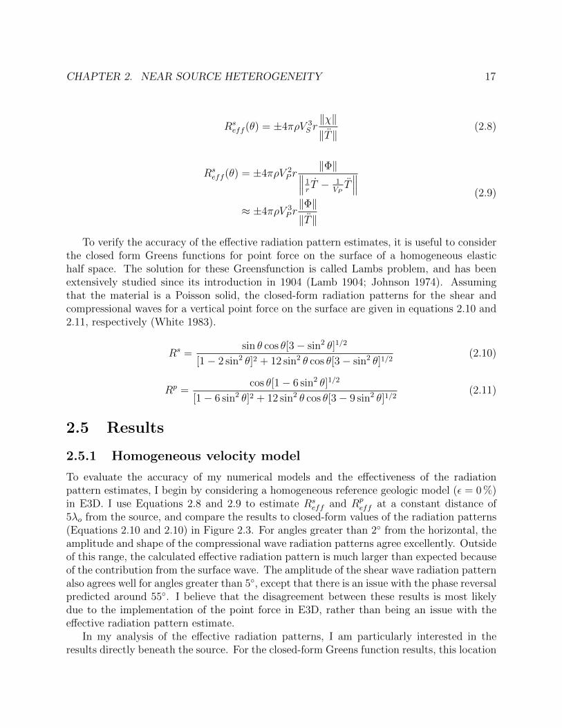
To verify the accuracy of the effective radiation pattern estimates, it is useful to considerthe closed form Greens functions for point force on the surface of a homogeneous elastichalf space. The solution for these Greensfunction is called Lambs problem, and has beenextensively studied since its introduction in 1904 (Lamb 1904; Johnson 1974). Assumingthat the material is a Poisson solid, the closed-form radiation patterns for the shear andcompressional waves for a vertical point force on the surface are given in equations 2.10 and2.11, respectively (White 1983).

Rs =sin θ cos θ[3− sin2 θ]1/2

[1− 2 sin2 θ]2 + 12 sin2 θ cos θ[3− sin2 θ]1/2(2.10)

Rp =cos θ[1− 6 sin2 θ]1/2

[1− 6 sin2 θ]2 + 12 sin2 θ cos θ[3− 9 sin2 θ]1/2(2.11)

2.5 Results

2.5.1 Homogeneous velocity model

To evaluate the accuracy of my numerical models and the effectiveness of the radiationpattern estimates, I begin by considering a homogeneous reference geologic model (ε = 0 %)in E3D. I use Equations 2.8 and 2.9 to estimate Rs

eff and Rpeff at a constant distance of

5λo from the source, and compare the results to closed-form values of the radiation patterns(Equations 2.10 and 2.10) in Figure 2.3. For angles greater than 2 from the horizontal, theamplitude and shape of the compressional wave radiation patterns agree excellently. Outsideof this range, the calculated effective radiation pattern is much larger than expected becauseof the contribution from the surface wave. The amplitude of the shear wave radiation patternalso agrees well for angles greater than 5, except that there is an issue with the phase reversalpredicted around 55. I believe that the disagreement between these results is most likelydue to the implementation of the point force in E3D, rather than being an issue with theeffective radiation pattern estimate.

In my analysis of the effective radiation patterns, I am particularly interested in theresults directly beneath the source. For the closed-form Greens function results, this location


0.2 0.4 0.6 0.8 1

30

210

60

90

120

150

330

180 0

φ (degrees)

R0.1 0.2 0.3 0.4 0.5

83

210

87

90

93

97

330

100 80

φ (degrees)

R

Figure 2.3: (left) Comparison of the effective radiation patterns, Rseff and Rp

eff , for thehomogeneous reference model (black) and the closed-form solution (red). (right) Close upview of the shear radiation patterns.

corresponds to the maximum compressional wave radiation and a node in the shear waveradiation. The numerical results also agree with this observation, except that there is asmall amount of shear radiation within the node. This unaccounted for energy is due toa combination of the near-field terms, which are not included in the closed form Greensfunction, and numerical noise in the model. As the distance to the source decreases, theratio between Rs

eff and Rpeff in the simulation increases significantly. I use this ratio as the

baseline for comparison between the homogeneous reference and the heterogeneous geologicmodels.

2.5.2 Isotropic fractal velocity models

In this section, I consider the results of several isotropic, heterogeneous geologic modelswithin a range of β and ε. For each of these models, I apply the same methodology in theprevious section to model the wavefield and calculate the effective radiation patterns. Thecalculated Rs

eff and Rpeff for a single model realization, with β = 1.7, ε = 1.5 %, and r = 5λo,

is compared to the results of the homogeneous reference model in Figure 2.4.As expected, there are significant variations from the homogeneous reference model,

although the average shape remains relatively unchanged. Note that because I do not requirethe velocity model to be axially symmetric, the effective radiation pattern is asymmetric. Inaddition, there is a significant increase in shear wave amplitude directly beneath the source.I also plot the value of Rs

eff/Rpeff , calculated throughout the model domain, in Figure 2.5.

I omit the areas in close proximity to the absorbing boundaries, because they may containa significant amount of numerical noise. The radial variations in this ratio, which tendto stabilize for z > 5λo, reflect the complex interaction of the wavefield with the modelheterogeneity. Another important observation is that Rs

eff/Rpeff within the shear wave node


0.2 0.4 0.6 0.8 1

30

210

60

90

120

150

330

180 0

φ (degrees)

R0.1 0.2 0.3 0.4 0.5

83

210

87

90

93

97

330

100 80

φ (degrees)

R


eff , for anisotropic heterogeneous model with β = 1.7, ε = 1.5 %, and r = 5λo (black), and thehomogeneous reference model (red). (right) Close up view of the shear radiation patterns.

x / λo

z / λ

o

-6 -4 -2 0 2 4 6

0

2

4

6

8

10 0.1

1

10

Rs/R

p

Figure 2.5: The Rseff/R

peff for an isotropic fractal model throughout the domain (β = 1.7

and ε = 1.5 %).


t (s)z

/ λo

0 10 20 30 400

2

4

6

8

10

Figure 2.6: Horizontal wavefield directly beneath the point source for an isotropic fractalmodel (β = 1.7 and ε = 1.5 %).

is increased significantly in this model.The increase in the shear wave energy beneath the source is likely due to scattering

of the shear wavefield, mode conversion of the compressional wavefield, and a near-fieldheterogeneity coupling effect. The timing character of this energy may give some insight asto its source: I expect that the contributions from scattering and mode conversion to bemostly incoherent and to not focus back towards the source location. In addition, I expectthat as the source-receiver distance increases, the relative contribution of mode conversionwill decrease, due to the lowering of the scattering angle. On the other hand, the near-fieldcoupling effect, which describes the interaction of the near-field energy with the heterogeneitynear the source, will likely produce a coherent shear wave arrival that will trace back towardsthe source. The horizontal wavefield, measured directly beneath the source for the modelrealization shown in the previous figures and corrected for spreading, is included in Figure2.6.

In these results, there is incoherent shear wave energy arriving immediately following thearrival of the direct P wave, which is the result of S-P-S mode-converted energy. Around theprojected arrival time of a direct shear wave from the source there is a coherent arrival thatI attribute to the near-field coupling term. In this case, the shape of the coherent arrivalis the same as is expected for the far-field arrivals. After this arrival, incoherent energycontinues to arrive in what would normally be identified as a coda wave, and is the result of


the scattered shear wave field.To explore the effect of the individual isotropic fractal parameters on the model results,

I begin by holding β constant at a value of 1.7, while I consider values of ε from 0 − 3 %.For each value of ε, I generate at least five independent, synthetic heterogeneous models,simulate the wave field using E3D, and calculate the effective radiation patterns beneaththe source. Because the variations in the effective shear radiation may differ by orders ofmagnitude for sets of β and ε, I choose to consider the log-average values of these resultsin my analysis. A plot of ratio of the shear to compression wave radiation as a function ofdepth and ε is given in Figure 2.7a. Note that because I am interested in contributions fromboth the coherenst and incoherent wavefield, I do not stack the individual realizations. Alsonote that, because of symmetry shear radiation directly beneath the source for ε = 0 % isexpected to be zero. However, due to the numerical limitations of the models, the estimatedshear radiation at this location is nonzero.

I observed that, over the range of ε considered in this analysis, the average value ofRseff/R

peff exceeds that of the reference model and increases with ε. As depth increases, this

ratio tends to increase with respect to the reference model until it reaches a steady value at5λo (the limit of the heterogeneous zone). In addition, the variation of these results decreaseswith depth, reflecting the self-averaging nature of this process (Muller and Shapiro 2001).The deviations seen for large depths and small ε are primarily due to boundary conditionissues.

Next, I investigate the effect of fractal exponent on the effective source radiation. Ichoose a range of β from 1.5 to 1.8, with a constant value of ε = 1.6 %. For each value of β, Iconsider at least five model realizations, and calculate the log average values. The resultingvalues of Rs

eff/Rpeff in this analysis are included in Figure 2.7b.

For this range of β, the variations in Rseff/R

peff are very small, and there are no trends

apparent in the results. For larger changes in β, I expect the dominant regime of scatteringto change and the character of the results to change dramatically (Browaeys and Fomel2009).

2.5.3 Layered fractal velocity models

While an isotropic fractal is a simple and useful model for many geologic media, a layeredfractal model is often more appropriate. This is especially the case for sedimentary structures,such as shale. To generate a layered model, I select values for fractal amplitude, ε, fractaldimension, β, and a horizontal scaling factor, b > 1 (see Equation 2.1). Figures 2.8 and2.9 show the effective radiation pattern and wavefield beneath the source for a model withε = 1.6 %, β = 1.7, and b = 10. In this model, I observe many of the same features as inthe isotropic case deviations from the radiation in the homogeneous model and an increasein shear wave energy beneath the source. However, compared to the isotropic model, theshear radiation beneath the source is decreased and the radiation at some lower angles isincreased.


0 2 4 6 8 10

10-2

10-1

100

z / λo

Rs /

Rp

0.0 %0.3 %0.8 %1.7 %2.5 %

(a)

0 2 4 6 8 10

10-2

10-1

100

z / λo

Rs /

Rp

Ref.1.51.61.71.8

(b)

Figure 2.7: (a) Effect of fractal amplitude (ε) on Rseff/R

peff beneath the source. (b)Effect of

fractal dimension (β) on Rseff/R

peff beneath the source.


0.2 0.4 0.6 0.8 1

30

210

60

90

120

150

330

180 0

φ (degrees)

R0.1 0.2 0.3 0.4 0.5

83

210

87

90

93

97

330

100 80

φ (degrees)

R


eff , for a layeredfractal model with ε = 1.6 %, β = 1.7, and b = 10 (black), and the homogeneous referencemodel (red). (right) Close up view of the shear radiation patterns.

t (s)

z / λ

o

0 10 20 30 400

2

4

6

8

10

Figure 2.9: Horizontal wavefield directly beneath the point source for a layered fractal model(ε = 1.6 %, β = 1.7, and b = 10).


0 2 4 6 8 10

10-2

10-1

100

z / λo

Rs /

Rp

0.0 %0.3 %0.8 %1.7 %2.5 %

Figure 2.10: Effect of fractal amplitude (ε) on Rseff/R

peff for a layered fractal model directly

beneath the source.

To evaluate the expected effect of heterogeneity shape on the effective radiation patterns,I vary ε similar to the previous section. I hold β at a constant value of 1.7, b at 10, vary εfrom 0− 3.3 %, and calculate the log-average Rs

eff/Rpeff for at least five model realizations.

The results of this analysis are given in Figure 2.10. Using a layered fractal model, thereare the same major trends as in the isotropic model. As ε increases, the expected value ofRseff/R

peff tends to increase, and as depth increases the variance decreases. A significant

difference between the results of the isotropic and layered models is that, for a given value ofε, a layered velocity model will produce twice the amount of shear wave beneath the sourceon average. Because I do not observe a strong dependence on β for the isotropic model, Iexpect the same for the layered models.

2.5.4 Reflecting velocity models

To evaluate whether the coherent shear wave pulse is useful for seismic imaging, I consideran isotropic fractal velocity model similar to those used in the previous sections, but with a30% lower average velocity in the upper layer. I use E3D to simulate the seismic wavefieldfrom a vertical point force on the surface of the model, and record the results for a verticaltrace beneath the source. The measured horizontal velocity for a model with ε = 1.6 % and


t (s)z

/ λo

0 10 20 30 400

2

4

6

8

10

Figure 2.11: Horizontal wavefield directly beneath the point force for a reflecting fractalmodel.

β = 1.7 is included in Figure 2.11.For a model with stacked homogeneous layers, I still expect a shear wave node to exist

beneath the vertical point source. However, as observed for the previous heterogeneousgeologic models, shear energy is introduced into this area from scattering, mode conversion,and near-source coupling effects. The coherent shear wave pulse in this model, and theincoherent arrivals around it, reflect off the interface at a depth of 5λo and may be tracedback to the surface. In addition to determining the location of the reflecting interface,geophysicists often attempt to determine the statistical characteristics of the geologic mediumthrough a statistical analysis of the travel time variations seen in reflection or refraction data(Iooss 1998; Kaslilar, Kravtsov, and Shapiro 2008). These additional shear waves containuseful information concerning the statistics of the source medium, as discussed in the previoussections, and may be used to supplement the seismic imaging applications.

2.6 Discussion

Approximate methods for solving the problem of elastic wave equation in heterogeneous me-dia, such as the Born approximation and RTT, are very efficient and effective at modelingthe effect of scattering, attenuation, and dispersion of waves. However, previous numericalinvestigations have discovered that shear wave energy, on the order of 10 % of the compres-


0 1 2 3 40

0.05

0.1

0.15

0.2

0.25

0.3

0.35

0.4

ε (%)

Rs /

Rp

IsotropicR

s / R

p = 1.2 ε

LayeredR

s / R

p = 0.5 ε

Figure 2.12: Correlations of ε and Rseff/R

peff for the isotropic fractal models (R2 = 0.98)

and layered fractal models (R2 = 0.99).

sional wave energy, may occur in these media that is not accounted for by the approximations(Przybilla and Korn 2008). The numerical analysis shows that, even for a small value of ε, asynthetic fractal geologic model is capable of producing this energy. I believe that becauseof the character and the timing of this additional shear energy, it is the result of S-P-S modeconversion and a near-source coupling effect. Two of the fundamental assumptions of theBorn and Rytov approximations prevent them from modeling these phenomena: These ap-proximations assume that the angle of scattering is either very high (backwards scattering) orvery low (forward scattering), which implies that mode conversion of the incident wavefield isnegligible. In addition, because each of these models rely on the far-field Greens functions asa reference, the interaction of the near-field term with the near source heterogeneity throughscattering and higher-order mechanical deformation (i.e. the near-field coupling effect) isoverlooked.

The results of my analysis suggest that I may develop some correlations between thisadditional shear energy introduced by these higher order terms, and the fractal characteristicsof the medium. A plot the log-average value of Rs

eff/Rpeff , measured in the far-field, as a

function of ε and fractal shape is given in Figure 2.12. There is a strong linear trend in theresults for both the isotropic fractal (R2 = 0.99) and layered fractal (R2 = 0.98) models.One may also draw some correlations between the characteristics of the coherent shear wave


pulse and the medium characteristics. The shape of this pulse does not vary significantlywith ε and β. However, as ε increases, the amplitude of the pulse tends to increase as isexpected.

The drop in the expected value of Rseff/R

peff for the layered velocity models is related

to the horizontal wavenumber scaling factor, b, in Equation 1. As b increases, the syntheticmodels are biased towards lower frequencies in the horizontal direction, and the average shapeof the heterogeneity changes from a sphere to an oblate spheroid. In effect, this reduces thedensity of vertically oriented velocity discontinuities in the model, which are important forthe horizontal scattering potential and the effectiveness of mode conversion of the primarywavefield.

Although I do not consider intrinsic anisotropy in my numerical models, one may drawsome conclusions about its expected effect on the shear wave radiation beneath the source.In anisotropic media, I expect that the wavefield energy will tend to focus in directions wherevelocity is maximum and will defocus where velocity is minimum (Tsvankin and Chesnokov1990; Tsvankin 1995). In my results, I expect the same trends: For a VTI medium withminimum velocity in the vertical direction, I expect a decrease in the shear energy generatedbeneath the source.

By comparing the trends in the results for ε and β (Figures 2.7a and 2.7b), I observe thatthe expected value of Rs

eff/Rpeff is much more sensitive to the choice of ε than β. This result

is expected because β influences the correlation of the heterogeneity within the medium,and therefore the character of the scattered wavefield. On the other hand, ε influencesthe amplitude of the heterogeneities, which will directly affect the amplitude of scattering.These effects are evident when attempting to invert for the fractal characteristics of anobject. While attempting to invert regional seismic data in the western Bohemia region,Klimes (2002) found that the inversion for the regional ε is both stable and reliable. Thismakes sense, considering the linear relationship observed between the scattered energy andε. Klimes also found that the inversion for the regional Hurst exponent, which is related toβ, is difficult and nonlinear. This observation is also supported by my analysis, as there didnot appear to be any straightforward trends in the results with β.

2.7 Conclusion

The interaction of the seismic wavefield with geological heterogeneity is commonly modeledusing the Born or Rytov approximations. However, due to basic assumptions about theheterogeneity characteristics, mode conversion, and the reference Greens functions, someaspects of the secondary wavefield are overlooked. I generate synthetic fractal models anduse finite differences to investigate the generation of additional shear waves directly beneatha point source on the surface. My results show that this shear energy increases linearlywith fractal amplitude and is not a strong function of fractal exponent. In addition, thepart of the additional shear energy that is coherent is due to a near-source coupling effect.These results have important implications for the predicted coverage of S-S seismic imaging,


because I have demonstrated that a significant amount of shear wave energy may be produceddirectly beneath the source without the need for a traditional shear source.

29

Chapter 3

Modeling Surface Wave-Based TunnelDetection Methods

3.1 Introduction

Tunnel and void detection is an important, yet challenging problem in geophysics and en-gineering, and it has important applications for the mining and transportation industries,public safety, and even domestic security. These range from determining the location ofold abandoned mine workings, karst features, to locating covert tunnels in sensitive areas;however, because there is often little to no surface expression of these features, conventionalmethods for locating them are limited to costly and time-consuming exploration drilling.Over the past several decades, researchers have applied geophysical methods ranging fromgravity and electrical resistivity to seismic diffraction in an attempt to identify voids. Inmany cases, these methods have been successful in determining the location of tunnels;however, they are often plagued with problems of low signal to noise ratios, non-uniqueinterpretations, and limitations with regards to geological heterogeneity.

3.2 Background on Void Detection Methods

In regions where the target void is large, shallow, and/or irregularly shaped (e.g. karst sink-holes), geophysicists tend to favor potential field geophysical methods such as microgravityand electrical resistivity (Butler 1984; Kaufmann, Romanov, and Nielbock 2011; Martinez-Moreno et al. 2013; Llopis et al. 2005; McCann, Jackson, and Culshaw 1987; Rybakov et al.2001; Schoor 2002). The observed anomalies resulting from these methods tend to be verysmall, often just above the survey resolution, and therefore tend to be most effective wherethe target is filled with water or air. Another significant challenge facing these methods isdue to the smoothness constraints required for their inversion, which tend to smear out thealready small anomalies (Riddle, Hickey, and Schmitt 2010). Some researchers have reportedsuccess in locating similar large or irregular objects using low-frequency GPR (Mochales et

CHAPTER 3. MODELING TUNNEL DETECTION 30

al. 2008). However, because of the relatively high frequencies required to locate smaller ob-jects and the highly attenuating materials in which they are located, the skin depth severelylimits the usefulness of EM methods (Llopis et al. 2005; Vesecky, Nierenberg, and Despain1980).

A range of seismic-based geophysical methods have been applied in an attempt to locatesubsurface voids. In comparison to gravity and resistivity, these are more suitable for smallerobjects with simpler geometries (e.g. tunnels). Body wave diffraction imaging is often pro-posed for detecting voids, especially where the target is deeply buried (Belfer et al. 1998;Peterie, Miller, and Steeples 2009; Sloan et al. 2010). In theory, this method should be ca-pable of detecting a tunnel, regardless of its depth. However, because the tunnel diffractionis limited to relatively high-frequencies, seismic skin depth is a severe limitation. In addi-tion, reflections and scattering from objects in the subsurface may easily obscure the targetdiffractions. The classic example for this application of diffraction imaging comes from USmilitarys attempts to locate tunnels excavated in the Korean DMZ (Vesecky, Nierenberg,and Despain 1980). Their investigation concluded that the wavelength of the seismic wavesrequired to detect the target tunnels is comparable to the average size of the local hetero-geneities. As a result, they would require an unreasonably detailed model of the local geologyfor this method to be useful.

In regions where the goal is to detect clandestine tunnels as they are being constructed(e.g. the US-Mexico border), researchers have proposed passive seismic detection methodsas an alternative (Sabatier and Matalkah 2008). Their goal is to listen for seismic sourcesassociated with excavation and blasting, which depending upon their type and frequencymakes this method potentially powerful. The primary concern for these methods is thatthey would rely upon large static seismic arrays recording continuously, and would requiresubstantial effort to monitor and process.

Because the targets of interest are often very shallow, other body wave-based methods,such as refraction or reflection, are not commonly applied. This is primarily due to surfacewaves interfering with the signals of interest. Researchers have noted in some cases, indirectobservations from these surveys may yield useful. For instance, using refraction tomography,an apparent decrease in raypath density may correspond to the targets location (Belfer et al.1998; Sloan et al. 2013).

In this study, I focus on seismic surface-wave void detection methods. Compared to bodywave diffraction, surface wave methods rely upon much lower frequencies, making them moreresistant to the effects of heterogeneity. Another major advantage to using surface wavesis that the inversion geometry is effectively limited to two dimensions, which significantlyreduces the computational requirements and makes the results simple to interpret. A numberof case-studies have reported success in locating shallow man-made tunnels using surfacewave backscattering (Ivanov et al. 2003; Sloan et al. 2010; Xia et al. 2007; Sherman, Rector,and Glaser 2014) and surface wave attenuation (Putnam et al. 2009; Sherman, Rector, andGlaser 2014). Korneev (2009) proposed a novel method for locating voids by identifying theemissions of Stoneley waves generated when a surface wave interacts with a fluid filled void.This approach is advantageous because it relies on a very persistent signal and because the


frequency content of the emitted wave may provide information regarding the size of the voidin addition to its location. Attempts to repurpose other traditional surface wave methods,such as MASW, are uncommon and rely upon indirect observations in a similar manner torefraction tomography (Sloan et al. 2013).

3.3 Surface Wave Methods and Geological

Heterogeneity

In this study I provide numerical support for the surface wave diffraction and surface waveattenuation-based void detection methods, and in particular I explore the limitations of thesemethods with regards to the depth of the target and the influence of geological heterogeneity.The effect of heterogeneity on wave propagation is commonly modeled using approximatesolutions to the stochastic wave equation or through numerical simulations (Shapiro andKneib 1993). The approximate methods, the two most common of which are the Born andRytov approximations, assume that velocity varies randomly as a function of position. Theseare very efficient and are commonly used where the incident wavefield and the geometry ofthe problem are simple, the magnitude of the heterogeneity is low, and the frequenciesof interest are relatively high (Chapman and Coates 1994; Marks 2006; Sato, Fehler, andMaeda 2012). In the case of surface wave tunnel detection, the wavefield is complex, theheterogeneity magnitude large, and the frequencies of interest low, which severely limits theusefulness of these methods.

Numerical simulations of wave propagation, using the Finite Difference or Finite Ele-ment methods, are direct solutions to the momentum equation. Because they do not relyupon assumptions regarding the amplitude or distribution of heterogeneity they are muchmore flexible than the approximate methods. In order to avoid problems with numericalinstability and dispersion effects, they require significant computational resources; however,this is offset by recent advances in inexpensive high-performance computing. I use the elas-todynamic wave propagation code, E3D, to simulate wave propagation in seismic tunneldetection experiments for a range of geometries and heterogeneous synthetic models (Larsenand Grieger 1998).

3.4 Case Study: Black Diamond Mines

As a reference point in this analysis, I selected a field site located in the Black DiamondMines Regional Preserve located near Antioch, California. Beginning in the 1850s this sitewas host to underground coal, underground sand, and surface sand mining operations. Thegeology is dominated by the Domengine formation, which has an upper unit composed ofa low-velocity sandstone and a lower unit composed of alternating mudstone, shale, andsiltstone (Sullivan and Sullivan 2012). The target void at this location is an abandonedadit, approximately 1.7 m in diameter and centered 4.3 m beneath the surface. Its exact


lateral location is unknown, and it is believed to filled with air. A group from the Universityof California Berkeley used a combination of microgravity and seismic surveys to attemptto find these features. The results of these geophysical surveys are discussed in detail inChapter 4.

3.5 Modeling Geologic Heterogeneity

One of the most common assumptions of geophysical models is that over some particularscale the earth may be adequately represented by discrete blocks of homogeneous material.This assumption is often necessary to facilitate useful work; however, extensive researchhas shown that the earth is heterogeneous over a wide range of scales (Browaeys and Fomel2009; Sato, Fehler, and Maeda 2012). This behavior is often modeled using self-affine fractalsbecause they are simple, and display scale invariance (Turcotte 1989).

To construct synthetic fractal models, I follow the methodology of Sherman et al. (2014).I begin by generating a matrix of normally distributed random values, apply the fractalfilter given by Equation 2.1, then sample and scale the results. The fractal distribution ischaracterized by a fractal amplitude, ε; fractal dimension, β; and scaling factors, ax, ay, andaz. ε describes the amplitude of the heterogeneity in the model, and is given as percentstandard deviation from the mean; β describes the way the heterogeneity is distributed inspace; and a describes the shape of the heterogeneity.

The preferred method for selecting ε and β in a synthetic model is through a carefulfrequency analysis of downhole geophysical measurements, such as a sonic log (Browaeysand Fomel 2009). In the absence of these direct measurements, an acceptable estimate of βmay be obtained by considering the geologic setting. The behavior of the scattered wavefieldis most sensitive to ε, and needs to be tuned accordingly (Sherman, Glaser, and Rector2014). As such, in this study I choose a single value of β, and vary ε when I investigate theeffect of heterogeneity on the void detection methods.

3.6 Numerical Analysis

I use the elastodynamic finite difference code E3D to model the interaction of the wavefieldwith the buried tunnel. E3D is developed at Lawrence Livermore National Laboratory, andit is 4th order accurate in space, 2nd order accurate in time, and uses a standard staggeredgrid formulation. It is been applied to solve problems ranging from earthquake simulation toseismic exploration, and is useful for modeling heterogeneous materials (Larsen and Grieger1998; Sherman, Glaser, and Rector 2014).

An illustration showing the geometry of the numerical models used in this analysis is givenin Figure 3.1. Each model is 60m long, 30m wide, 30m deep, and has a grid size of 0.08m.The embedding medium has an average Vp = 1.5 km/s, Vs = 1 km/s, and a ρ = 2.3 g/cm3.Each heterogeneous model used in this analysis is based upon an independent realization of


Figure 3.1: Block diagram showing numerical model geometry and a single realization of thefractal heterogeneity (β = 1.7, ε = 2 %).

a fractal model in Vp, with β = 1.7, and ε = 0− 8%. I maintain a single degree of freedomin these models by applying a constant Vp/Vs and density. The target void is a cylindricaltunnel, with a diameter of 1.7m and depth to the tunnel axis ranging from 4− 12m.

In the Black Diamond case study the adit is believed to be filled with air, which hasan estimated Vp = 0.35 km/s, Vs = 0 km/s, and ρ = 0.0013 g/cm3 at STP. Because theimpedance contrast between air and the background medium is very large, this introducespotential instabilities into the numerical simulations. To overcome this I artificially reducethe impedance contrast in two steps: First, I increase the density of the air within the tunnelto 1 g/cm3. Applying this heavy air reduces the impedance contrast to a more manageablelevel for the numerical simulations. Second, I linearly grade the seismic velocities and densityof these materials over eight gridpoints outwards from the tunnel boundary to further smooththe gradient in impedance in the model.

A free-surface boundary condition is applied to the top, and an absorbing (Claytonand Engquist) boundary condition is applied to the sides and bottom of each model. Tominimize undesired reflections from the absorbing boundaries, I apply a severely attenuatingmaterial to the along the side and bottom of each model. In addition, I found that placing aheterogeneous material within range of an absorbing boundary could result in unpredictablenumerical errors. To overcome this problem, I damp the heterogeneity within four gridpointsof the model boundaries.

For the seismic source, I apply a point force to the top of the model as indicated inFigure 3.1. The source shape is the integral of a Ricker wavelet with a nominal centerfrequency of 100Hz. Because I am interested in the Rayleigh wavefield, I record the verticalparticle velocity along the surface of the model perpendicular to the tunnels central axis.Simulations were conducted on a single workstation using the OpenMPI protocol, with each


model completed in approximately one day.

3.7 Theory

Because of the very large contrast between the embedding medium and a target void, whichis often filled with air or water, surface waves are a useful tool for determining a voidslateral location. In this study, I focus on the effectiveness of surface wave backscattering andattenuation-based void detection methods.

3.7.1 Surface Wave Backscattering

Surface wave backscattering occurs when the wave interacts with a void and then reflectsbackwards towards the seismic source. Because the surface waves decays exponentially withdepth for a given wavelength, the amplitude of the backscattered wave is very sensitive to thedepth of the target. Significant backscattering may still occur where the source wavelengthis much greater than the size of the void (Sloan et al. 2010).

In some cases, the backscattered waves are identifiable in an unprocessed seismic record;however, they are often obscured by the coda of the forward propagating wavefield. Toisolate the backscattered wavefield, I use a methodology adapted from Sloan et al. (2010).I begin by applying amplitude gain control (AGC) and geometric spreading correctionsto the data, use a directional f-k filter to remove the forward propagating energy, and thenremove the previous AGC. Finally, I inspect the resulting seismic record to identify any wavespropagating backward towards the source at the Rayleigh wave velocity. The apparent originof the backscattered waves should correspond to an edge of the buried void. Because theresearch presented here is numerical, I am not limited by sampling constraints or undesirednoise in the results. For field applications, it is necessary to apply a lowpass filter to thedata before the f-k filter to avoid spatial aliasing in the results. In addition, for noisyrecords, stacking the results for multiple shots after a linear moveout (LMO) correction willsignificantly improve the signal to noise ratio (Sherman, Glaser, and Rector 2014).

If a Stoneley wave is excited in the target by the forward propagating wavefield, it willemit a slowly-decaying, resonant wave back into the ground (Korneev 2009). On a seismicrecord, this will appear as a set of traces parallel to the primary forward and backscatteredwavefield. To isolate these, I use the same procedure described above for the backscatteredwaves, which will isolate the source of the backward propagating part of this wavefield andimprove the estimate of the void location.

3.7.2 Surface Wave Attenuation

In the previous section, I considered the direction and source of the waves, and in contrast,for the surface wave attenuation analysis I consider the patterns in amplitude as they interactwith the target. I first consider a case where the target extends infinitely in the out-of-plane


direction (i.e. a tunnel) and wavelength of interest is greater than the targets depth. As thesurface wave passes across the tunnel, I expect that its amplitude will decrease significantlyover a distance proportional to the targets size. Another important case to consider is wherethe void is limited in the out-of-plane direction. For a ray traveling directly through the void,the amplitude will drop as it passes over it. However, for a ray passing near the edge of thevoid, there will be an observed increase in its amplitude that occurs as the wave flows aroundthe target. As the distance and the angle from the void increases the observed increases ordecreases to the surface wave amplitude become less severe.

As before, the drop in surface wave amplitude is often apparent in unprocessed seismicrecords, but may be obscured by seismic noise. To isolate these anomalies, I generate anattenuation curve for the numerical survey as follows: I correct the data for geometricspreading effects and apply a 3-pole Butterworth bandpass filter to the seismic data. Then,assuming an average surface wave velocity, I window the data around the projected wavearrival and estimate the amplitude or energy. In this study, I calculate the L2-norm eachwindowed trace to estimate the arriving energy, E. Finally, I select some reference near thesource with energy, Eo, and normalize the data and plot the results versus distance.

To determine the location of the target within the seismic array, I look for significantdeviations from the average trend of the attenuation curve (i.e. assuming a constant back-ground Q). Lacking other information, these deviations could be interpreted as a suddenincrease in the rate of attenuation. Note that, while it is possible to obtain an estimate oflocal Q by assuming a characteristic length scale in the survey, this may be unstable in thepresence of noise. As such, I choose to limit the interpretation to the amplitude domain.

3.7.3 Effect of Void Size and Depth

To arrive at a rough estimate of the surface wave energy drop due to crossing the void, whichis also proportional to the amplitude of the backscattered wavefield, I consider a simple modelwhere there is a total reflection or absorption of the surface wave over the voids cross-section.Using an exponential model for the incident surface wave energy with depth, I obtain anestimate of the energy drop, ∆E, by integrating with depth as illustrated in Equations 3.1and 3.2.

∆E ∝∫ h+r

h−re−az/λdz (3.1)

∆E ∝ exp(−ah/λ) · sinh(ar/λ) (3.2)

Here r is the radius of the void, and h is the depth to the central axis of the void, λis the wavelength of interest, and a is a scaling parameter. As expected, the result is anexponential function of both tunnel depth and radius scaled by wavelength. The depth ofthe target is the primary limiting factor for this method for two reasons: First, becausemany of the tunnels of interest are designed for human use, their size will fall into a limited


range. Second, even if a tunnel radius is a small fraction of the wavelength, from experience,I know that it will still produce a strong effect on the incident wavefield.

3.8 Results

To demonstrate the effectiveness of the surface wave-based void detection methods, I presentthe results of homogeneous and heterogeneous background models, with each modeled afterthe abandoned adit at Black Diamond Mine site. I evaluate the effect of tunnel depth andwavelength, heterogeneity amplitude, and the effect of angle of incidence on these methods.

3.8.1 Homogeneous Background Model

Figure 3.2a shows the measured wavefield for a numerical simulation with a tunnel buriedin a homogeneous background. The seismic source is located on the surface of the model at−30m and has a center wavelength of 5m; the tunnel is centered at a depth of 3.4m andhas a radius of 1.7m. Note that the scale of Figure 3.2a is saturated to emphasize the laterarriving phases. The record is dominated by the direct Rayleigh wave, which arrives at thetunnel (offset = 0m) around 30ms. At this point, some energy is captured by the tunnel,and the rest is partitioned between a backscattered wave traveling towards the source and anattenuated transmitted wave moving forward to the opposite edge of the model. After thepassage of the direct Rayleigh wave, I observe a persistent resonant phase traveling at theRayleigh wave velocity and originating from the tunnel, which is the result of the Stoneleywave excited within the tunnel. I also observe two reflections from the side and end of themodel, which are the result of imperfect absorbing boundaries.

After applying the AGC and the f-k filter to attenuate forward propagating energy, Iobtain the wavefield given in Figure 3.2b. Here I observe that the backscattered Rayleighwave and the backward traveling portion of the resonant phase have been amplified signif-icantly. Both of these terminate and flatten near the location corresponding to the tunnelaxis (offset = 0m). The surface wave attenuation curve for this model, which is normalizedby the energy measured at an offset of −20m, is given in Figure 3.3. A sudden drop in thesignal occurs at an offset of −5m, which corresponds to an apparent increase in the rate ofattenuation. The curve stabilizes after an offset of 6− 7m, suggesting a return to a normalrate of attenuation.

In field data, the approximate location of the tunnel would be indicated by the originof the backscattered energy, and by the center of the attenuating region. Note that evenfor this ideal case, the precision of these methods is limited to about 1− 2m the horizontaldirection. Because of the asymmetry in the anomalies, which is apparent in Figure 3.3, theestimate of the void location may also be biased away from the source. To remedy this, Isuggest that the source be placed on both sides of the target, and the results averaged.


Offset (m)

Tim

e (m

s)

-30 -20 -10 0 10 20 30

0

10

20

30

40

50

60

70

80

90

100

(a)

Offset (m)

Tim

e (m

s)

-30 -20 -10 0 10 20 30

0

10

20

30

40

50

60

70

80

90

100

(b)

Figure 3.2: (a) Measured Vz along the top of the model for a homogeneous backgroundmaterial. (b) Measured Vz along the top of the model for a homogeneous background materialafter applying AGC and the directional f-k filter.


-20 -15 -10 -5 0 5 10 15 20

0.3

0.4

0.5

0.6

0.7

0.8

0.9

1

Offset (m)

E/E

o

Figure 3.3: Surface wave attenuation curve for a model with a homogenous backgroundmaterial.

3.8.2 Heterogeneous Background Model

Figure 3.4a shows the measured wavefield for the same geometry as in the previous case,except that the background material is heterogeneous with β = 1.7 and ε = 4 %. Again, thedominant direct Rayleigh wave, the backscattered Rayleigh wave, and the resonant emissionfrom the tunnel are all present. The most notable change here is the superposition of theRayleigh wave coda, which is most evident near the seismic source for low values of time.

The backward propagating wavefield for this model is shown in Figure 3.4b. In additionto the direct backscattered Rayleigh wave and resonant emission from the tunnel, the surfacewave energy is backscattered off of the heterogeneity in the background model. In this case,the location of the tunnel corresponds to the apparent source of the largest observed phases.The surface wave attenuation curve for this model is given in Figure 3.5. For comparison,I also include the attenuation curve for this same model before the tunnel is excavated. Asexpected, there are small variations in each curve that are the consequence of the backgroundheterogeneity in the model. Despite this, the attenuation curve for the model including thetunnel clearly departs from the average trend at −5m and recovers after 7− 8m.

For this particular realization of a heterogeneous geologic model, the approximate locationof the tunnel is still evident from the surface wave attenuation and backscattering methods.However, in the case of the attenuation method the anomalous region is broader and more


Offset (m)

Tim

e (m

s)

-30 -20 -10 0 10 20 30

0

10

20

30

40

50

60

70

80

90

100

(a)

Offset (m)

Tim

e (m

s)

-30 -20 -10 0 10 20 30

0

10

20

30

40

50

60

70

80

90

100

(b)

Figure 3.4: (a) Measured Vz along the top of the model for a heterogeneous background ma-terial (β = 1.7, ε = 2 %). (b) Measured Vz along the top of the model for the heterogeneousbackground material after applying AGC and the directional f-k filter.


-20 -15 -10 -5 0 5 10 15 20

0.3

0.4

0.5

0.6

0.7

0.8

0.9

1

Offset (m)

E/E

o

Figure 3.5: Surface wave attenuation curve for a model with a heterogeneous backgroundmaterial with (solid) and without (dotted) the buried tunnel.

biased away from the source. In the case of the backscattering method, the origin of thebackscattered waves is less clear. The result is an overall decrease in resolution and precisionfor the void detection methods.

3.8.3 Effect of Void Depth and Location

Because the anomaly in the surface wave attenuation method associated with the void iseasily quantifiable, I focus on it to determine the limitations of each method with regardsto the tunnel depth and the wavelength of interest. Assuming that the background mediumis homogeneous, I look at the attenuation curve for a set of models with tunnels buried atdepths ranging from 4 − 12m, with a constant radius of 1.7m. I run each model for meansource frequencies ranging from 0.10−0.20 kHz, which correspond to dominant wavelengthsfrom 9 − 4.5m, respectively. The measured attenuation curves for these models are shownin Figures 3.6a, 3.6b, and 3.7a. For a given mean source frequency, the drop in amplitudedecreases with increasing tunnel depth. I determine the maximum deviation for each modelaway from the predicted attenuation curve (assuming a homogeneous model with no tunnel),∆E, and scale the depth by the mean wavelength, λo.

The scaled results from the numerical analysis are shown in Figure 3.7b. As predictedby Equation 3.2, the observed anomaly for the surface wave attenuation method decreases


-20 -15 -10 -5 0 5 10 15 200

0.1

0.2

0.3

0.4

0.5

0.6

0.7

0.8

0.9

1

Offset (m)

E/E

o

456789101112

(a)

-20 -15 -10 -5 0 5 10 15 200

0.1

0.2

0.3

0.4

0.5

0.6

0.7

0.8

0.9

1

Offset (m)

E/E

o

456789101112

(b)

Figure 3.6: Effect of tunnel depth on surface wave attenuation curve for a mean frequencyof (a) 100Hz, (b) 150Hz.


-20 -15 -10 -5 0 5 10 15 200

0.1

0.2

0.3

0.4

0.5

0.6

0.7

0.8

0.9

1

Offset (m)

E/E

o

456789101112

(a)

0 0.5 1 1.5 2 2.5 30

0.05

0.1

0.15

0.2

0.25

0.3

0.35

0.4

0.45

0.5

Depth / λo

∆E

(b)

Figure 3.7: (a) Effect of tunnel depth on surface wave attenuation curve for a mean frequencyof 200Hz. (b) The maximum deviation from the predicted attenuation curve for scaleddepth.


exponentially with scaled depth, and at z/λo = 1 the anomaly is about 5 %. Under idealconditions, I would expect to detect a tunnel using these methods that is buried a depth lessthan one wavelength under the surface.

3.8.4 Effect of Heterogeneity

To determine the limitations of the surface wave void detection methods with regards togeological heterogeneity, I again focus on the surface wave attenuation curve. I assume thatthe tunnel is buried at a constant depth of 3.4 m with a radius of 1.7m, and assume thatthe background medium is characterized by fractal parameters β = 1.7 and ε = 0−8 %. Theattenuation curves for 24 independent heterogeneous model realizations are given in Figure3.8a.

As expected, as the heterogeneity amplitude (ε) increases, the variance in the attenua-tion curve increases. For ε4 %, the variations in the attenuation curve due to heterogeneityapproach the amplitude of the tunnel anomaly, limiting the usefulness of a single result.However, if the surface wave attenuation curve is measured at multiple locations across thetunnel and the results averaged, it is possible to extend the useful range of the methodsignificantly. In this study, this is equivalent to averaging the independent realizations fordifferent values of ε. The averaged attenuation curves for models different levels of hetero-geneity are given in Figure 3.8b. Using this approach, the tunnel is clearly identified up toε = 4 %; however, as ε continues to increase, the likelihood that a tunnel will be detecteddecreases. For the limiting case with ε = 8 %, I was unable to detect the tunnel in any modelrealization.

An interesting phenomenon occurs in models with moderate heterogeneity (ε ≈ 2− 3 %).While the attenuation curve anomaly for a single heterogeneous realization is often lower inamplitude, the average tunnel anomaly increases noticeably. This suggests that the presenceof some small heterogeneity in a system may increase the capability of the surface wavedetection methods.

3.8.5 Effect of Array Geometry

In the each of the previous models, it was assumed that the virtual string of geophones wasoriented normal to the tunnels central axis. To determine the effect of a non-normal incidenceangle on the detection methods, I consider two additional models where the wavefield ismeasured at every point on the surface of the model. I estimate the energy arriving ateach point, and then sample the results along virtual geophone strings oriented from 0− 30

(measured from the normal to the tunnel axis). The corresponding attenuation curves fora homogeneous model and a heterogeneous model are included in Figures 3.9a and 3.9b,respectively. For angles greater than 0, there is a very small, almost negligible increase inthe attenuation curve associated with the tunnel, which occurs because the surface wavesencounter a tunnel with a larger apparent size.


-20 -15 -10 -5 0 5 10 15 20

0.5

1

1.5

2

2.5

Offset (m)

E/E

o

(a)

-20 -15 -10 -5 0 5 10 15 20

0.3

0.4

0.5

0.6

0.7

0.8

0.9

1

Offset (m)

E/E

o

0.5%1%2%4%

(b)

Figure 3.8: (a) Surface wave attenuation curves for models with heterogeneity amplitude, ε,ranging from 0.5− 4 %. (b) Mean surface wave attenuation curves for different values of ε.


-20 -15 -10 -5 0 5 10 15 20

0.3

0.4

0.5

0.6

0.7

0.8

0.9

1

Offset (m)

E/E

o

0o

10o

20o

30o

(a)

-20 -15 -10 -5 0 5 10 15 20

0.3

0.4

0.5

0.6

0.7

0.8

0.9

1

Offset (m)

E/E

o

0o

10o

20o

30o

(b)

Figure 3.9: Surface wave attenuation curves measured at different angles from the tunnelaxis for an (a) homogeneous background model, (b) heterogeneous background model.


3.9 Discussion

In this analysis, I focus on the attenuation method to determine the limitations of surfacewave void detection. Due to the conservation of energy within the system, the drop insurface wave energy as it travels across the void should be proportional to the amplitude ofthe backscattered surface waves. As such, I expect that the backscattering method to beeffective under the same conditions as for the attenuation method.

As a rule of thumb, these methods are capable of detecting a void that is buried lessthan one wavelength beneath the surface and for objects much smaller than the wavelength.Due to their dependence on source wavelength, a frequency-based analysis of the results mayprovide an estimate for void depth. Because the surface wave attenuation method relies uponcareful windowing to avoid extraneous energy and the surface wave backscattering methoddoes not lend itself to frequency-domain analysis, I suggest that this should be done in thetime-domain by applying successive bandpass filters to the data.

For heterogeneous geological media, I expect that these methods will be effective for εless than about 6 %. The observed increase in the average attenuation curve for moderateheterogeneity is the result the increased wavefield complexity. The mechanism for this in-crease may be related to a concept from information theory called dithering (Wannamakeret al. 2000). Before an analog signal is quantized, a small amount of noise (dither) is addedto it, and by doing so correlatable quantization errors are attenuated. The result is that theaverage noise floor of the digital signal is decreased, and the effective resolution is increased.In a similar manner, the wavefield dither may attenuate correlated energy from the surfacewave coda, thereby increasing the tunnel anomaly within the attenuation curve.

3.10 Conclusion

The surface wave backscattering and attenuation methods are useful tools for determiningthe location of voids, such man-made tunnel, buried less than one wavelength beneath thesurface. The advantages over other methods, such as body wave diffraction, are that theyrequire minimal processing and are straightforward to interpret. As such, surface wave-basedmethods are prime candidates for field interpretation and for use over wide areas. Movingforward, my goal is to extend this analysis to include voids with a limited horizontal extent,to investigate other possible survey geometries, and to apply other processing techniquessuch as attenuation tomography to the data. The results of this work is being applied toimprove the geophysical surveys designed to detect the buried adit at Black Diamond MinesRegional Park, and I am investigating other sites to apply surface wave-based void detectiontechniques.

47

Chapter 4

Tunnel Detection Case Study at BlackDiamond Mines

4.1 Introduction

Near-surface tunnel and void detection is an important, yet challenging problem in geophysicsand engineering. It has applications in the mining and transportation industries, and is ofgreat concern for public safety and national security. In the past, a number of geophysicalmethods have been proposed as tools to detect these objects: potential field methods, suchas microgravity and electrical resistivity; traditional seismic exploration methods, such asseismic refraction and diffraction imaging; and surface wave-based methods, such as Rayleighwave attenuation and backscattering.

Potential field detection methods are commonly applied to detect large, irregularly shapedcavities, such as sinkholes and other features in karstic terrain (Butler 1984; Kaufmann, Ro-manov, and Nielbock 2011; Martinez-Moreno et al. 2013; McCann, Jackson, and Culshaw1987; Mochales et al. 2008; Riddle, Hickey, and Schmitt 2010; Rybakov et al. 2001; Schoor2002). A significant challenge for these methods is that their associated geophysical anoma-lies tend to be very small, often just above the noise-level. In addition, the smoothnessconstraints required by their inversion smears out the anomalies in space, further increasingthe level of difficulty for interpretation. As such, potential field methods are only effectivewhere the target is very large, close to the surface, and filled with a high-contrast material.

Traditional seismic exploration methods, such as body wave diffraction and reflection, aremore common where the target is small and has a regular geometry, such as with man-madetunnels (Belfer et al. 1998; Ivanov et al. 2003; Peterie, Miller, and Steeples 2009; Sloan et al.2010; Vesecky, Nierenberg, and Despain 1980). However, the useful range of these methodsis severely limited by practical concerns: For shallow targets, the seismic phases of interestmay be obscured by near-surface refractions and surface waves. For deeper targets, theconcern is that these methods rely on relatively high-frequency waves, which are susceptibleto geologic heterogeneity and have a limited depth of penetration.

CHAPTER 4. TUNNEL DETECTION AT BDM 48

I employ surface wave-based void detection methods and limited microgravity data tolocate near-surface tunnels within the Black Diamond Mines Regional Preserve near Antioch,California. Using surface waves to detect tunnels has a number of advantages over otherseismic methods (Ivanov et al. 2003; Putnam et al. 2009; Sherman, Rector, and Glaser 2014;Sloan et al. 2013; Xia et al. 2007): First, surface waves are often the largest arrivals in aseismic record, and are therefore straightforward to isolate. Second, the seismic frequenciesrequired to detect the target are much lower than the corresponding body-wave methods,making them more resistant to naturally occurring, high-frequency geologic heterogeneity.Third, the geophysical anomalies associated with tunnels are often very large and may beapparent on unprocessed seismic records, which reduces the need for intensive processingand complicated interpretation.

4.2 Description of Field Study

4.2.1 Black Diamond Mines Regional Preserve

In this case study, I discuss seismic and microgravity data collected within the Black Dia-mond Mines Regional Preserve (BDM), which is located near Antioch, California. A mapshowing its location is given in Figure 4.1. This region is named for its underground coalmining operations, which began in the 1860s and continued through the early 20th century.Beginning in the 1920s the industry shifted towards underground silica sand mining, andlater towards surface sand mining. In total, approximately 1.8 million tons of sand weremined at BDM until operations ceased in 1949. The East Bay Regional Park Service cur-rently manages the land, and has developed BDM into a mining museum (EBRPD 2012).

The predominant geologic unit at the experimental site is a white, quartz-rich sandstoneunit in the lower Domengine formation (Sullivan and Sullivan 2012). The sandstone isextremely friable, has a very low seismic velocity (VS ≈ 300m/s), and is highly attenuating(Qs < 10). In addition, there is a thin, dipping coal seam at an approximate depth of27m. There are a number of significant mining-related features at this site: First, thelower tunnel (LT), which is located within the sandstone unit at a depth of about 20m(measured from the central axis), with a diameter of 2m. Its exact lateral location and stateof repair are unknown. Second, the upper tunnel (UT), which is buried at a depth of 4.7m,is approximately 3.3m in diameter, and is the primary target of the analysis. The laterallocation of this tunnel is well constrained by historical survey records, and is believed to beintact and filled with air. The experimental site is located within an old surface sand miningexcavation, which has since been reclaimed for recreational use. During 1998, park officialsnoted a subsidence pit in the area, which was thought to be the result of a stoping failure ofthe lower tunnel. The pit has since been backfilled, and the perceived source of the failuregrouted. Figures 4.2a and 4.2b show a simplified diagram of the sites geometry. In 2012there was a smaller stoping failure that was surface filled. The relationship of this failurewith the mine workings in unknown (McKanna 2013).


123˚W 122.5˚W 122˚W 121.5˚W

37˚N

37.5˚N

38˚N

38.5˚N

BDM

Figure 4.1: The experimental site (BDM) is located within the Black Diamond Mines Re-gional Preserve, near Antioch, California, USA.

4.2.2 Instrumentation

Seismic data were collected using 24 vertical spiked 14Hz geophones manufactured by Geo-metrics. The geophones are damped 50 %, have a flat response to 250Hz, and were sampledat 2000Hz. All seismic sources were generated by swinging a 20− lb sledge hammer into analluminum plate placed on the ground. The data collection and initial processing were per-formed by a group of undergraduate and graduate students from the University of CaliforniaBerkeley.

For the seismic survey, the geophones were deployed in two distinct configurations, asindicated in Figure 4.2a. The first configuration is the linear array (L-Array), which wasoriented approximately north-south across the tunnel axis, with geophones spaced 3m (10 ft)apart. Seismic sources were placed at a spacing of 15.2m (50 ft) along the array, with amaximum offset of 76.2m (250 ft) to the north side of the array. The second configurationis the rectangular array (R-Array), which has 19 geophones placed across the tunnel axisand 5 geophones parallel to the tunnel. The geophones in the R-Array were spaced at 2.3m


UT

LTL-Array

R-Array

20m

N

(a)

Pit

Stope

UT

LT5m

5m

(b)

Figure 4.2: (a) A plan view representation of the experimental site, which shows the locationof the linear seismic array (L-Array), rectangular seismic array (R-Array), the upper tunnel(UT), and the lower tunnel (LT). The location of the upper tunnel is known from historicalsurvey data, and the exact location of the lower tunnel is unknown. (b) A cross-sectionview of the site, which shows the approximate locations of the upper and lower tunnels,the subsidence pit that opened in 1998, and the proposed location of the stoping failureassociated with the pit.


(7.5 ft), and seismic sources were placed on the opposite legs of the rectangle spaced at 1.0m(3.25 ft). In addition to the seismic data, a limited set of microseismic data were collectednear the anticipated location of the upper tunnel. These were collected using a LaCosteRomberg G-meter along a line oriented parallel to the L-Array, with a spacing of about 3m.

4.3 Theory / Processing

Because of the very large contrast in shear modulus between the earth and a target void,surface waves are useful tools for determining their location. While the geophysical anomaliesthat indicate the presence of such an object are often apparent in an unprocessed seismicrecord, I suggest a few minor processing steps to amplify them. In the following sections,I discuss the theory and processing for the three complimentary seismic methods used inthe study: surface wave backscattering, 1D surface wave attenuation, and 2D surface waveattenuation tomography. I also briefly discuss the application of microgravity data at BDM.

4.3.1 Surface Wave Backscattering

Surface wave backscattering occurs when a traveling wave encounters an object with suffi-cient impedance contrast, which causes a portion of the surface wave to reflect backwardstowards its source. Even for simple void geometries, the amplitude of the reflected wavesis difficult to calculate because of a fundamental assumption made in the analysis of sur-face waves: that they propagate along the surface of a homogeneous or layered half-space.However, considering that, in absence of a void, a surface wave will have an amplitude thatdecreases exponentially with depth, one may estimate the reflection amplitude assuming atotal reflection of the wave over the targets depth cross section. This result suggests thatthe reflection is proportional to an exponential function of void depth, the wavelength ofinterest, and to a lesser extent void radius (Sloan et al. 2010; Sherman, Rector, and Glaser2014). A numerical analysis of surface wave backscattering from tunnels by Sherman et al.(2014) suggests the limiting case for this method is a target buried one wavelength beneaththe surface.

While in many cases it is possible to see evidence of a backscattered wavefield from anunprocessed seismic record, I use the following processing steps that were adapted fromSloan et al. (2010) and Sherman et al. (2014). First, I collected seismic data using theL-Array for multiple shots on a single side of the region of interest. I applied a causal 3-poleButterworth bandpass filter, with corner frequencies of 2.5 and 10Hz, to the data. Note thatthis corresponds to a mean wavelength of about 50m, which is 10 times the upper tunnelspredicted depth. Next I applied spreading corrections and AGC to the data, and thenapplied an f-k filter designed to attenuate the entire forward propagating wavefield. Finally,I applied an LMO correction to each shot assuming an average surface wave velocity, stackeach shot, and plot the resulting wavefield. If a backscattered wavefield is present, it will


appear as a coherent surface wave traveling backwards towards the source with its origincorresponding to the approximate tunnel location.

Another phenomenon of interest for the surface wave backscattering analysis is the emis-sion of resonant seismic waves from the target void. These waves may be excited whenan incident wave interacts with a fluid filled object, and are of interest because they decayslowly and may contain information regarding the targets size (Korneev 2009). Using therecommended processing steps for the backscattering analysis, the backward propagatinghalf of the resonant wavefield will be isolated and serves to improve the accuracy of thelocation estimate.

4.3.2 1D Surface Wave Attenuation

The analysis of surface wave attenuation data is the direct compliment to the surface wavebackscattering analysis. While in the previous section I considered the arrival times of surfacewaves to determine the location of voids, for the attenuation analysis I instead considertheir observed amplitude as they interact with the target. In the case of a tunnel thatextends a long distance in the out of plane direction, I expect to observe a drop in amplitudeproportional to the wavelength of interest as it passes the tunnels central axis. Sherman etal. (2014) also considered the problem of surface wave attenuation in their numerical study,and found this method is best suited for targets buried less than one wavelength beneaththe surface.

Again, depending on the tunnel depth and frequency of interest, the drop in amplitudemay be apparent on an unprocessed seismic record. To further isolate these features, Igenerated a surface wave attenuation curve using the following procedure: First, I collectedseismic data using the same geophone array and shots in the backscattering analysis andapply the same bandpass filter (from 2.5−10Hz) and geometric spreading corrections to thedata. Next, I applied a rectangular window to the data around the projected Rayleigh wavearrival time, and estimate the maximum amplitude of the wave at each geophone. For eachshot, I normalized the measured amplitudes by the value measured at the geophone nearestto the source. Finally, I averaged the results of each shot, and plot as a function of distance inthe array. If successful, the location of the target void will correspond to a sudden deviationfrom the average trend of the curve, which in the absence of other information could beinterpreted as a sudden increase in rate of attenuation. Note that, while it is possible todirectly estimate the value of Q by assuming some characteristic length, I prefer to interpretthe results in the amplitude domain because of its stability.

4.3.3 2D Surface Wave Attenuation Tomography

To extend the surface wave backscattering analysis to multiple dimensions, I consider thesurface wave amplitude patterns using an array of geophones surrounding the target region(as opposed to a dense array passing over it). As before, for rays passing through the target,I expect to observe a drop in the surface wave amplitude proportional to the wavelength of


interest. However, for rays passing along the edge of the target, there may be an apparentincrease in the surface wave amplitude due to energy flowing around the target.

The data for the 2D surface wave attenuation analysis were collected using the R-Arrayshown in Figure 4.2a. In this array, the geophones are placed on two adjacent sides formingan L shape and seismic sources are placed on the opposite sides forming a rectangle. Iestimated the amplitude of the arriving Rayleigh wave for each source-receiver pair using thesame procedure from the 1D analysis. To diminish the effect of varying source amplitudeand coupling, I used a seismic source spacing equal to half of the geophone spacing andaverage the results for adjacent shots. Next, I considered a simplified model with a constantbackground quality factor, Q, and source amplitude, Ao. I used linear regression to estimatethese values, and then reject source-receiver pairs more than ±2.5 standard deviations fromthe trend to improve the stability of the analysis.

To invert for Q within the array, I began by discretizing the domain into 2.5×2.5m voxels,and used a straight-ray approximation and the objective function described in Equation 4.1:

C =

∥∥∥∥ln

(AiAo

)+

fπ

VRQXi

∥∥∥∥+ αGQ (4.1)

Here, Ai is the observed Rayleigh wave amplitude for the ith source-receiver pair; f is themean frequency of the bandpass filter, VR is the average Rayleigh wave velocity, Q is a vectorcontaining the quality factor estimates, Xi is a vector containing the distance through eachvoxel, α is a scaling factor, and G is the smoothness operator. I restricted the acceptablevalues of Q to range between 0.1 and 10 and use a maximum step size of 0.01. To perform theinversion, I used the COBYLA (constrained optimization by linear approximation) algorithmin the Python optimization toolbox for a maximum of 1000 steps. Finally, I plotted the Qestimates in space and searched for discrete regions with lower than average Q, which maycorrespond to the location of the target object.

4.3.4 Microgravity

Although the focus of this study is on surface wave-based methods, I chose to collect asmall amount of microgravity data at the BDM site. These data were collected along thesection of the L-Array nearest to the supposed location of the upper tunnel, and wereprocessed to recover the Bouguer anomaly with applied terrain corrections and regionaltrend removed. To determine the estimated amplitude of the gravity anomaly, I modeledthe tunnel as a buried cylinder with depth and radius equal to the values estimated bythe park management. Assuming that the tunnel is filled with air, the expected maximumgravity anomaly is approximately 0.15mGal for the upper tunnel and 0.03mGal for thelower tunnel. Considering the survey geometry and instrumental limitations, it is possibleto observe the anomaly for the upper tunnel.


(a) (b)

Figure 4.3: (a) An example of the seismic data collected using the L-Array, with the sourceoffset 15.2m to the north of the array. These data have been corrected for geometric spread-ing and are for the frequency range of 2.5 to 10Hz. [The south end of the array correspondsto a distance of 0m.] (b) Seismic records from the L-Array that have been processed toemphasize surface wave backscattering. The primary backscattered waves are highlighted inred, and the resonant emissions are highlighted in blue. The two apparent sources of thesewaves are located at a distance of 40 and 58m from the south end of the array.

4.4 Results

An example of the seismic data collected using the L-Array is shown in Figure 4.3a. Thisdata is for a single shot offset 15m to the north of the array, and it has been processed toremove the effects of geometric spreading and has been filtered to retain frequencies from 2.5to 10Hz. From this record, it is clear that the dominant phase is the Rayleigh wave, whichpropagates relatively unperturbed until it reaches a distance 40m from the south of thearray. After this point, there is a sudden and severe decrease in the surface waves amplitudethat suggests that this geophone corresponds to the location of the upper tunnel. Anotherimportant feature in this record is observed within the coda of the direct Rayleigh wave.There are subtle indications of backscattered energy from 40 to 60m from the south of thearray, although their source is unclear.


(a)

15 20 25 30-0.2

-0.15

-0.1

-0.05

0

0.05

Distance (m)

Gra

vity A

no

ma

ly (

mG

al)

(b)

Figure 4.4: (a) The measured surface wave attenuation curve for the L-Array. There aresignificant deviations from the average trend at a distance of about 35m and 65m fromthe south of the L-Array. (b) A plot of the limited microgravity data versus distance fromthe south side of the L-Array. There is an anomaly of about 0.15mGal near the expectedlocation of the upper tunnel (Distance ≈ 22m).


Figure 4.5: The inverted values of Q from the 2D surface wave attenuation analysis (thesouthwest corner of the R-Array is located at [0, 0]m). There are two discrete regions oflow-Q observed within the array.


The seismic record given in Figure 4.3b shows the result of further processing of L-Arrayseismic data to amplify the backscattered wavefield. This record includes data from five shotsoffset from 15 to 76m to the north side of the array, and has had the LMO correction removedto facilitate a direct comparison with the record in Figure 4.3a. The wavefield processingreveals a prominent source of backscattered surface wave energy near at a distance of 40m,and a smaller source near 58m. An interesting feature here is that after the passage ofthe initial backscattered wave there is a decaying harmonic wave traveling backwards atthe Rayleigh wave velocity, which is evidence of a Stoneley wave being excited within thetunnels. This is a useful feature for identifying the source of the backscattered waves, andmay yield information regarding the size of the target void.

The same seismic data from the L-Array, this time processed into an attenuation curve,is given in Figure 4.4a. In the absence of the two tunnels, I would expect to see a smoothexponential curve with terminating a value of A/Ao ≈ 0.4 at a distance of 100m for thefrequency range of interest and the expected Q within the Domengine sandstone. From theattenuation curve, I observe major drops from the expected trend around 35 and 65m fromthe south end of the array. These locations of increased apparent attenuation correspond tothe sources of backscattered surface wave energy observed in Figure 4.3b.

Extending the surface wave attenuation analysis to 2D using the R-Array, I obtain theinverted values of Q shown in Figure 4.5. For this site, the best-fit background value of Qis approximately 4.5. There are two discrete regions where the value of Q is abnormally low(≈ 2.0). The first is located from 7.5 to 15m from the south and spans the width of the R-Array. The second is located 27−40m from the south, and is limited to the right side of thearray. The northern edges of these regions corresponds with the highly attenuating regionsobserved in Figure 4.4a and the sources of backscattered surface wave energy observed inFigure 4.3b.

The measured microgravity anomaly for the BDM site is given in Figure 4.4b. Althoughthese data are too sparse to interpret on their own, the larger of the two inverted low-Qregions corresponds to the 0.15mGal gravity anomaly observed at a distance of 22m.

4.5 Discussion

Figure 4.6 highlights the regions with abnormally low-Q and/or density, the location of thetwo sources of backscattering determined from the above analyses, and my interpretation ofthe two target tunnels location. The location of the larger low-Q anomaly and the largersource of backscattering (B0) correspond to the estimated location of the upper tunnelprovided by the BDM management, and the amplitude of the gravity anomaly agrees withtheir estimates of the tunnels depth, size, and state. The location of the smaller low-Qanomaly and the smaller source of backscattering (B1) may correspond to the location ofthe lower tunnel. The stoping failure observed in 1998 at the site and the subsequentremediation efforts may give insight into the limited size of the low-Q anomaly. The anomaly


Low Q

Low Q, ρ

20m

B0

B1

N

Figure 4.6: A schematic showing the locations of the low-Q regions observed in the 1Dand 2D surface wave attenuation analyses, the location of the backscatterers (B0 and B1)observed in the surface wave backscattering analysis, and the low density region observed inthe microgravity analysis. My estimates of the location of the upper and lower tunnels areindicated.

may correspond to the section of the tunnel that remained open following the failure, and themissing section of low-Q material may correspond to a failed section that was later grouted.

The choice to use the frequency band of 2.5 − 10Hz, which corresponds to a meanwavelength (λo) of about 50m, in my analysis is significant. The numerical simulations ofsurface wave void detection completed by Sherman et al. (2014) suggests that the maximumtarget depth for these methods is z/λo < 1 and that the minimum tunnel diameter isd/λo 1. At BDM I am considering values of z/λo ≈ 0.1 and d/λo ≈ 0.07 for the uppertunnel, and z/λo ≈ 0.4 and d/λo ≈ 0.04 for the lower tunnel. Both of these tunnels fallinto the acceptable range and both were located successfully in my analysis, which lendssupport to these estimates of the methods range. As the result of the very high intrinsicattenuation of the Domengine formation sandstone, I was unable to recover much higherseismic frequencies and were unable to further test the z/λo limit. However, in theory acareful frequency-based analysis may be used to estimate the depth of target voids at otherlocations. While this could be achieved in the frequency domain, there may be issues withphases other than the direct Rayleigh wave polluting the results. Therefore, I suggest that


this analysis be completed in the time domain through the careful application of sequentialfilters.

4.6 Conclusion

In this case study, I employed surface wave attenuation, surface wave backscattering, andlimited microgravity void detection methods to locate two tunnels within the Black DiamondMines Regional Preserve. These methods are fast to perform, simple to interpret, andrequire minimal processing, which makes them useful for field interpretation. In addition,my work agrees with the numerical study of surface wave-based void detection methods bySherman et al. (2014), which suggests that these methods will be successful for voids buriedwithin one wavelength of the surface and with wavelength much larger than the voids size.Moving forward, I am working to incorporate these surface wave detection methods at otherlocations, implementing a frequency-based analysis to estimate the depth of these features,and am considering further applications of the resonant Stonely wave emissions from voids.

60

Chapter 5

Conclusion

5.1 Modeling Geological Heterogeneity

Although it is often overlooked in geophysical analyses, heterogeneity is an important featureof geologic materials. Throughout this dissertation, I have developed a methodology formodeling this heterogeneity using a fractal model. A major benefit of this model is itssimplicity - only two independent parameters (fractal dimension, β, and fractal amplitude, ε)are required to characterize an isotropic material, and three additional parameters (scalingfactors, ax, ay, and az) are required to characterize a more general anisotropic material.Where available, these parameters may be estimated directly from geophysical data such aswell-log measurements (see Figures and ). Otherwise, they may be estimated by consideringthe depositional environment (Browaeys and Fomel 2009).

Another important feature of the heterogeneity model used in my research is scale invari-ance, which implies that it is not possible to determine the scale of an observation withoutan external reference. This feature is illustrated by the model realizations shown in Figures1.4a through 1.5d, which could potentially characterize anything from a hand specimen toan entire geologic formation. The major consequence of this for my research is that I am ableto generalize my results by carefully selecting scaling factors, such as the dominant seismicwavelength.

The major challenge for modeling a heterogeneous material is the non-trivial computa-tional effort. Because it is not possible to have a perfect knowledge of a materials structureand because closed-form solutions may break down in the presence of complexity and , itis often necessary to rely upon multiple stochastic realizations of a model and numericalsimulation techniques. In my research I have worked extensively with the Finite Differencecode E3D to model wave propagation in heterogeneous media. A large part of this researchhas been devoted to developing a Python-based interface to E3D that handles heterogeneousmodel creation, simulation management, and post-processing (see Appendix A).

CHAPTER 5. CONCLUSION 61

5.1.1 Shear Wave Generation

In Chapter 2, I investigate a phenomenon involving shear wave generation from seismic pointforces on the surface. Here, an expert in the geophysical exploration industry reported thatcoherent shear waves were being generated within the shear wave node of the sources dur-ing a VSP test, which were unexplained by current theory. To investigate this problem, Iconducted an extensive numerical study of this test using my heterogeneity model and E3D.My results suggest that the rogue shear waves are the result of a complex interaction of thenear-field wavefield term with near-surface heterogeneity. This case study highlights anothermajor benefit of using a heterogeneous model for geophysical investigations. Higher-orderfeatures of wave propagation, such as scattering, scattering attenuation, coda wave gener-ation, and mode conversion, are often ignored in analyses. By applying my heterogeneousmodel to the analysis, these features arise naturally in the simulations (for example, seeFigure 2.6).

5.1.2 Near Surface Tunnel Detection

In Chapters 3 and 4, I discuss the results of a numerical analysis and field study of seismictunnel detection methods. In particular, I focus on surface wave-based methods and howgeological heterogeneity effects their resolution. My results show that these methods are veryeffective in determining the location of underground features buried up to one wavelengthbeneath the surface. They also demonstrate how considering a heterogeneous model (seeFigure 3.4a) that is calibrated against field observations (see Figure 4.3a) may help to identifyimportant phenomena in “real-world” data, extend the results to other situations, and revealunexpected behavior. An example of this is seen in how the surface wave attenuation curvebehaves in the presence of heterogeneity: This method tends to be very resistant to moderatelevels of heterogeneity, and may actually see an increase in resolution in heterogeneous media(see Figure 3.8b).

5.2 Future Work

Moving forward, I plan to pursue applications for modeling wave propagation in heteroge-neous geologic media, and to extend my approach to model other physical processes in thesemedia such as fracture propagation and fluid flow. In addition, because it has importantapplications in the transportation, exploration, and security industries, I plan to continuedeveloping my surface wave-based tunnel and void detection methodology. Up to this point,I have focused primarily on using a linear array geometry to detect long, shallow tunnelspassing perpendicular to the array. I would like to increase the reliability of my method byincluding a more general 2D array geometry into the analysis. In addition, I plan to exploreadditional case studies and determine ways to extend my method to detect other features,such as underground bunkers or collapse features.

62

Appendix A

PyE3D Manual

Prerequisites

• Python 2.7

• Numpy

• Scipy

• Matplotlib

• E3D binary

• ffmpeg codec (optional, required for video output)

• OpenMPI (optional, required for multicore processing)

Installation

PyE3D is an open-source project by Christopher Sherman at the University of CaliforniaBerkeley designed to serve as a Python-based graphical user interface to the Finite Differencecode E3D. Note that the E3D code is developed by Shawn Larsen and Lawrence LivermoreNational Laboratory, and is not available as part of this package.

To install PyE3D, begin by installing the prerequisites, downloading the source codelocated at: https://github.com/cssherman/PyE3D, and placing these files in a convenientlocation. From the command line, run the python file e3d gui.py. If this is the first time theGUI has been opened, there will be a command-line prompt asking for a username, whichis used to help organize files on the hard drive. Finally, once the GUI opens, go to theadvanced tab and set the appropriate paths for the input/output files and the E3D binary.

APPENDIX A. PYE3D MANUAL 63

Some important notes:

1. If you would like to use email alerts, you should edit the function e3d gmail, whichis located in the file e3d functions.py, and change the example gmail login criteriafromaddr and passwd to match your desired values before running the GUI.

2. This code is designed and tested to run for a Unix-style operating system. Somemodifications to the code may be necessary to work in a Windows environment.

Basic PyE3D Usage

To begin call the file e3d gui.py from the terminal, which will open the PyE3D GUI in anew window (see Figure A.1). The purpose of this GUI is to create a configuration file(./e3d default.pkl), which is sent to the program, e3 main.py. This is the bulk of the workis done to build models, communicate with E3D, and process the results. At the top of theGUI there are seven tabs that step through the model configuration process. These include:

• Main (basic model setup, boundary conditions, analysis options)

• Advanced (timesteps, material control, paths)

• Materials (material velocity, density, statistics, geometry)

• Sources (source location, type, frequency)

• Traces (seismograph output locations, types)

• Movies (movie output locations, types)

• Rendering (decimation, plot saturation, etc.)

At the base of the window, there are six buttons that are used to start the analysis andmanage configuration files. These include:

• Run PyE3D: This sends the current configuration file to e3 main.py and starts theanalysis

• Run Post: This triggers any post-processing that is requested in the Rendering tab(targets the files specified under the “Linking Directory”)

• Save: This saves the current configuration of the GUI to the file ./e3d default.pkl

• Export: This exports the current GUI configuration to a user-specified location

• Load: This reads the user-specified configuration file and updates the GUI


• Restore: This loads the default settings for the configuration file, which are found ine3d classes.py.

While running the function e3d main.py, the results will be stored in the location spec-ified by the “Output Location”, which is defined under the Advanced tab. The directorystructure created is as follows: [output location]/[username]/[date of simulation inD−M−Y format]/[model number]/. This directory may contain the following files:

• ./E3D in.txt: The main file sent to the E3D code

• ./[property].pv: Files containing the velocity model structure

• ./wav.sac: The file containing the custom input wavelet

• ./sac/: A folder containing seismograph outputs

• ./mov/: A folder containing movie outputs

To organize longer series of simulations, each of these directories are linked to the locationspecified under “Linking Directory”, which is defined in the Advanced tab: [linking directory]/[model number]/.

Main Tab

The Main tab (Figure A.1)contains information about the basic setup of the model: modelsize, origin of first grid point, spacing of the grid, and model runtime. The units of theseparameters should be consistent: if distance is specified in kilometers then the model timeshould be in seconds, and if distance is specified in meters then model time should be inmilliseconds.

The primary boundary conditions for the model are defined here: reflecting, absorbing,and surface (absorbing boundary conditions on the lower/side of the model and free surfaceat z=0). A sponge boundary condition artificially damps the wavefield within a few gridpoints of the model edge (it can be very inefficient and is not recommended by the developersof E3D). An attenuating boundary condition places a layer of severely attenuating materialon the edge of the model (this is more efficient than the sponge condition).

Other items on this page include the option to run the model, choose an elastic/acousticmodel, turn attenuation on/off, or select a 2D/3D model. Note that a 2D model is definedin the X-Z plane (Y=0).


Figure A.1: PyE3D GUI Main Tab


Advanced Tab

The Advanced tab (Figure A.2) contains other options for model setup, material control,and defines the important paths:

• Timestep size: this the ratio of the dt used in the model to the Courant condition (ct).This number should be less than one (preferably ≤ 0.1)

• Number of runs: this defines the number of times the model should run (generating anew realization at each step)

• MPI nodes: these values describe the way the problem should be discretized for Open-MPI processing. If nX=nY=nZ=1, the program will default to the single core option.

• Independent parameters: this describes how many parameters to generate an indepen-dent stochastic fractal realization

• Model generation: the options are to create a new model, link to an old model, or toedit an old model.

• Output location: This is the path to place outputs from PyE3D

• Logfile Location: This is where PyE3D places logs the work done

• Linking Directory: The path where PyE3D will place links to the files

• E3D Path: The path to the E3D binary

• Input Name: What PyE3D names the input file sent to E3D

• Alert address: The address where PyE3D will send alerts to


Figure A.2: PyE3D GUI Advanced Tab


Materials Tab

The Materials tab (Figure A.3) controls the material properties, the statistical distributionof their heterogeneities, and their geometry. A tab for each material region is included atthe top. When generating a model, PyE3D will run through each of these in sequence andwill overwrite the model in the specified region. At the bottom of the tab are buttons toadd a new region (placed at the end), remove region (current selection), and to render themodel. The p-wave velocity, s-wave velocity, and density are defined by their average valueand percent standard deviation. The material attenuation are defined by the p-wave ands-wave quality factors.

The material properties in each region may be specified to be homogeneous, independentrandom, or fractal. A fractal distribution is defined by its fractal dimension, which describesthe degree of correlation between regions, and by three scaling parameters, which describethe shape of the heterogeneities. Note that for fX = fY = fZ = 1, the result is an isotropicfractal, and for fX = fY > fZ the result is a layered fractal in the z-direction.

The options for defining a regions geometry are as follows:

• Entire Domain: region fills the entire model (by default this should be Region 1).

• Rectangle: region is specified by the x,y,z coordinates of two opposing corners.

• Sphere: region is specified by the x,y,z coordinates of the center and the radius.

• Cylinder: region is specified by the x,y,z coordinates of the to ends of the cylinder anda radius.

• Polynomial Surface: region is specified below [a0 + a1*x + a2*x**2]*[b0 + b1*y +b2*y**2]

• Planar Surface: region of thickness (T) beneath a plane that is specified by an x,y,zcoordinate, its strike (S), dip (D), roughness wavelength (L), and roughness amplitude(A).

• Open box: region of N-gridpoints around the edge of the model are specified.

• Interp: imports a file in X-Y-Z-V format and interpolates it into the model space.


Figure A.3: PyE3D GUI Materials Tab


Sources Tab

The Sources tab (Figure A.4) defines the type and characteristics of the seismic sources inthe model. At the top of the model are tabs for each specified source, and at the bottom arebuttons to add and remove sources. The options for source types include:

• P: pure compressional wave force

• S: pure shear wave force

• Moment Tensor: specified by 6-independent components of the moment tensor

• Point Force: specified by a unit force vector

• Point Fault: specified by strike, dip, rake

• Finite Fault: specified by strike, dip, rake, length, width, depth, hypocenter, andrupture velocity

The options for the wavelet include a Ricker wavelet and the derivative of a Gaussian.Amplitude is specified in units of dyne or dyne-cm. The center frequency of the wavelet isspecified in units of Hz (or kHz if length units are given in meters). The offset from timet=0 is specified by O.


Figure A.4: PyE3D GUI Sources Tab


Traces Tab

The Traces tab (Figure A.5) defines the seismograph outputs for the model. At the top aretabs listing each set of traces, and at the bottom are buttons to add/remove traces. Eachtrace is defined by its direction, the x,y,z coordinates of the origin, number of measurementpoints, spacing, and spreading corrections.

Figure A.5: PyE3D GUI Traces Tab


Movies Tab

The Movies tab (Figure A.6) defines the movie outputs for the model. At the top are tabslisting each movie specified, and at the bottom are buttons to add/remove movies. Theplane of the movie is specified by a direction and position.

Figure A.6: PyE3D GUI Movies Tab


Rerendering Tab

The Rendering tab (Figure A.7) controls the behavior of the Run Post option. Here, youcan select which types of outputs to render, the degree to decimate the results in time andspace, and the saturation of the outputs.

Figure A.7: PyE3D GUI Rerendering Tab


E3D Classes / Update Function

Another important note to discuss is the file e3d classes.py. The format and default valuesfor the configuration file, which is written in .pkl format, are defined here. Of special notehere is the update method for the Config class. This method is called before each modelis generated and sent to E3D. To instruct PyE3D to change its behavior between loops, Irecommend including the code here. For instance, to update the average p-wave velocity ofMaterial 1 between steps, you could insert the following code:

def update ( s e l f , loop ) :s e l f . path . log msg = ”Test %s ” % loop # Write a message

tmp = [ 3 . 0 , 3 . 1 , 3 . 2 , 3 . 3 , 3 . 4 , 3 . 5 ] # Model spaces e l f . mate r i a l [ 0 ] .mn[ 0 ] = tmp [ loop ] # Update the average p−v e l

76

Bibliography

Aki, K. and B. Chouet (1975). “Origin of coda waves: Source, attenuation, and scatter-ing effects”. In: Journal of Geophysical Research 80.23, pp. 3322–3342. doi: 10.1029/JB080i023p03322.

Aki, K. and P. G. Richards (2002). Quantitative seismology. University Science Books.Baig, A. M., F. A. Dahlen, and S. H. Hung (2003). “Traveltimes of waves in three-dimensional

random media”. In: Geophysical Journal International 153.2, pp. 467–482. doi: 10.1046/j.1365-246X.2003.01905.x.

Barton, C. C. and P. R. Le Pointe (1995). Fractals in petroleum geology and earth processes.Springer.

Belfer, I. et al. (1998). “Detection of shallow objects using refracted and diffracted seismicwaves”. In: Journal of Applied Geophysics 38.3, pp. 155–168. doi: 10.1016/S0926-

9851(97)00025-6.Browaeys, T. J. and S. Fomel (2009). “Fractal heterogeneities in sonic logs and low-frequency

scattering attenuation”. In: Geophysics 74.2, WA77–WA92. doi: 10.1190/1.3062859.Butler, D. K. (1984). “Microgravimetric and gravity gradient techniques for detection of

subsurface cavities”. In: Geophysics 49.7, pp. 1084–1096. doi: 10.1190/1.1441723.Chapman, C. H. and R. T. Coates (1994). “Generalized Born scattering in anisotropic me-

dia”. In: Wave Motion 19.4, pp. 309–341. doi: 10.1016/0165-2125(94)90001-9.EBRPD (2012). Black Diamond Mines Regional Park. East Bay Regional Park District. url:

www.ebparks.org/parks/black_diamond.Frankel, A. and R. W. Clayton (1986). “Finite difference simulations of seismic scattering:

Implications for the propagation of short-period seismic waves in the crust and models ofcrustal heterogeneity”. In: Journal of Geophysical Research 91.B6, pp. 6465–6489. doi:10.1029/JB091iB06p06465.

Hardage, B. (2012). Personal Communication.Iooss, B. (1998). “Seismic reflection traveltimes in two-dimensional statistically anisotropic

random media”. In: Geophysical Journal International 135.3, pp. 999–1010. doi: 10.

1046/j.1365-246X.1998.00690.x.Ivanov, J. et al. (2003). “Seismic search for underground anomalies”. In: SEG Expanded Ab-

stracts. Society of Exploration Geophysicists, pp. 1223–1226. doi: 10.1190/1.1817502.

BIBLIOGRAPHY 77

Johnson, L. R. (1974). “Green’s Function for Lamb’s Problem”. In: Geophysical Journal ofthe Royal Astronomical Society 37.1, pp. 99–131. doi: 10.1111/j.1365-246X.1974.tb02446.x.

Kaslilar, A., Y. A. Kravtsov, and S. A. Shapiro (2008). “Geometrical Optics of AcousticMedia with Anisometric Random Heterogeneities: Travel-Time Statistics of Reflected andRefracted Waves”. In: Advances in Geophysics. Ed. by R. Dmowska. Vol. 50. Elsevier.Chap. 4, pp. 95–121.

Kaufmann, G., D. Romanov, and R. Nielbock (2011). “Cave detection using multiple geo-physical methods: Unicorn cave, Harz Mountains, Germany”. In: Geophysics 76.3, B71–B77. doi: 10.1190/1.3560245.

Klimes, L. (2002). “Estimating the Correlation Function of a Self-affine Random Medium”.In: Pure appl. geophys. 159.7-8, pp. 1833–1853. doi: 10.1007/s00024-002-8711-1.

Korneev, V. (2009). “Resonant seismic emission of subsurface objects”. In: Geophysics 74.2,T47–T53. doi: 10.1190/1.3068448.

Lamb, H. (1904). “On the Propagation of Tremors over the Surface of an Elastic Solid”. In:Philosophical Transactions of the Royal Society of London. Series A, Containing Papersof a Mathematical or Physical Character 203, pp. 1–42. doi: 10.2307/90855.

Larsen, S. and J. Grieger (1998). “Elastic modeling initiative, part III: 3-D computationalmodeling”. In: SEG Expanded Abstracts.

Levander, A. R. and N. R. Hill (1984). “Finite-difference simulations of noise problemscaused by near-surface heterogeneity”. In: SEG Expanded Abstracts, pp. 392–395. doi:10.1190/1.1893992.

Llopis, J. L. et al. (2005). “Tunnel Detection Along the Southwest U.S. Border”. In: Sym-posium on the Application of Geophysics to Engineering and Environmental Problems.EEGS, pp. 430–443. doi: 10.4133/1.2923487.

Marks, D. L. (2006). “A family of approximations spanning the Born and Rytov scatteringseries”. In: Optics Express 14.19, pp. 8837–8848. doi: 10.1364/OE.14.008837.

Martinez-Moreno, F. J. et al. (2013). “Combined microgravity, electrical resistivity tomog-raphy and induced polarization to detect deeply buried caves: Algaidilla cave (SouthernSpain)”. In: Engineering Geology 162, pp. 67–78. doi: 10.1016/j.enggeo.2013.05.008.

McCann, D. M., P. D. Jackson, and M. G. Culshaw (1987). “The use of geophysical surveyingmethods in the detection of natural cavities and mineshafts”. In: Quarterly Journal ofEngineering Geology and Hydrogeology 20.1, pp. 59–73. doi: 10.1144/GSL.QJEG.1987.020.01.06.

McKanna, J. (2013). Personal Communication.Mochales, T. et al. (2008). “Detection of underground cavities by combining gravity, magnetic

and ground penetrating radar surveys: a case study from the Zaragoza area, NE Spain”.In: Environmental Geology 53.5, pp. 1067–1077. doi: 10.1007/s00254-007-0733-7.

Muller, T. M. and S. A. Shapiro (2001). “Most probable seismic pulses in single realizations oftwo- and three-dimensional random media”. In: Geophysical Journal International 144.1,pp. 83–95. doi: 10.1046/j.1365-246x.2001.00320.x.

BIBLIOGRAPHY 78

Muller, T. M., S. A. Shapiro, and C. M. A. Sick (2002). “Most probable ballistic waves inrandom media: a weak-fluctuation approximation and numerical results”. In: Waves inRandom Media 12.2, pp. 223–245. doi: 10.1088/0959-7174/12/2/305.

Nishizawa, O. and Y. Fukushima (2008). “Laboratory Experiments of Seismic Wave Propa-gation in Random Heterogeneous Media”. In: Earth Heterogeneity and Scattering Effectson Seismic Waves. Vol. 50. Elsevier, pp. 219–246.

Nishizawa, O. and G. Kitagawa (2007). “An experimental study of phase angle fluctuation inseismic waves in random heterogeneous media: time-series analysis based on multivariateAR model”. In: Geophysical Journal International 169.1, pp. 149–160.

Peterie, S. L., R. D. Miller, and D. W. Steeples (2009). “Diffraction Imaging Versus ReflectionProcessing For Shallow Void Detection”. In: SEG Expanded Abstracts.

Przybilla, J. and M. Korn (2008). “Monte Carlo simulation of radiative energy transfer incontinuous elastic random mediathree-component envelopes and numerical validation”.In: Geophysical Journal International 173.2, pp. 566–576. doi: 10.1111/j.1365-246X.2008.03747.x.

Przybilla, J., M. Korn, and U. Wegler (2006). “Radiative transfer of elastic waves versus finitedifference simulations in two-dimensional random media”. In: Journal of GeophysicalResearch: Solid Earth 111.B4, pp. 566–576. doi: 10.1029/2005JB003952.

Putnam, N. H. et al. (2009). “Attenuation Analysis of Rayleigh Waves Used to LocateShallow Manmade Tunnels”. In: Proceedings of the 43rd U.S. Rock Mechanics Symposium& 4th U.S. - Canada Rock Mechanics Symposium.

Riddle, G. I., C. J. Hickey, and D. R. Schmitt (2010). “Subsurface Tunnel Detection UsingElectrical Resistivity Tomography and Seismic Refraction Tomography: A Case Study”.In: Symposium on the Application of Geophysics to Engineering and Environmental Prob-lems, pp. 552–562. doi: 10.4133/1.3445481.

Rybakov, M. et al. (2001). “Cave detection and 4-D monitoring: A microgravity case historynear the Dead Sea”. In: The Leading Edge 20.8, pp. 896–900. doi: 10.1190/1.1487303.

Sabatier, J. M. and G. M. Matalkah (2008). “A Study on the Passive Detection of ClandestineTunnels”. In: 2008 IEEE Conference on Technologies for Homeland Security, pp. 353–358. doi: 10.1109/THS.2008.4534477.

Saito, T. (2006). “Velocity shift in two-dimensional anisotropic random media using theRytov method”. In: Geophysical Journal International 166.1, pp. 293–308. doi: 10 .

1111/j.1365-246X.2006.02976.x.Saito, T. et al. (2003). “Simulating the Envelope of Scalar Waves in 2D Random Media

Having Power-Law Spectra of Velocity Fluctuation”. In: Bulletin of the SeismologicalSociety of America 93.1, pp. 240–252. doi: 10.1785/0120020105.

Sato, H., M. C. Fehler, and T. Maeda (2012). Seismic Wave Propagation and Scattering inthe Heterogeneous Earth : Second Edition. Springer.

Schoor, M. van (2002). “Detection of sinkholes using 2D electrical resistivity imaging”. In:Journal of Applied Geophysics 50.4, pp. 393–399. doi: 10.1016/S0926-9851(02)00166-0.

BIBLIOGRAPHY 79

Shapiro, S. A. and G. Kneib (1993). “Seismic Attenuation By Scattering: Theory and Nu-merical Results”. In: Geophysical Journal International 114.2, pp. 373–391. doi: 10.

1111/j.1365-246X.1993.tb03925.x.Shapiro, S. A., R. Schwarz, and N. Gold (1996). “The effect of random isotropic inhomo-

geneities on the phase velocity of seismic waves”. In: Geophysical Journal International127.3, pp. 783–794. doi: 10.1111/j.1365-246X.1996.tb04057.x.

Shearer, P. M. and P. S. Earle (2008). “Observing and Modeling Elastic Scattering in theDeep Earth”. In: Advances in Geophysics. Ed. by R. Dmowska. Vol. 50. Elsevier. Chap. 6,pp. 167–193.

Sherman, C. S., S. D. Glaser, and J. W. Rector (2014). “The effects of near source hetero-geneity on shear wave evolution”. In: Geophysics 79.4, pp. 1–9. doi: 10.1190/GEO2013-0199.1.

Sherman, C. S., J. Rector, and S. D. Glaser (2014). “Tunnel detection using surface wave-based methods (Under review)”. In: Geophysics -.-, pp. –.

Sloan, S. D. et al. (2010). “Void Detection Using Near-Surface Seismic Methods”. In: Ad-vances in Near-surface Seismology and Ground-penetrating Radar. Ed. by R. D. Miller,J. H. Bradford, and K. Holliger. Society of Exploration Geophysicists, American Geo-physical Union, Environmental and Engineering Geophysical Society. Chap. 12, pp. 201–218.

Sloan, S. D. et al. (2013). “Using near-surface seismic refraction tomography and multichan-nel analysis of surface waves to detect shallow tunnels: A feasibility study”. In: Journalof Applied Geophysics 99, pp. 60–65. doi: 10.1016/j.jappgeo.2013.10.004.

Sullivan, R. and M. D. Sullivan (2012). “Sequence Stratigraphy and Incised Valley Archi-tecture of the Domengine Formation, Black Diamond Mines Regional Preserve and theSouthern Sacramento Basin, California, U.S.A”. In: Journal of Sedimentary Research82.10, pp. 781–800. doi: 10.2110/jsr.2012.66.

Tsvankin, I. (1995). “Body-wave radiation patterns and AVO in transversely isotropic me-dia”. In: Geophysics 60.5, pp. 1409–1425. doi: 10.1190/1.1443876.

Tsvankin, I. et al. (2010). “Seismic anisotropy in exploration and reservoir characterization:An overview”. In: Geophysics 75.5, 75A15–75A29. doi: 10.1190/1.3481775.

Tsvankin, I. D. and E. M. Chesnokov (1990). “Synthesis of body wave seismograms frompoint sources in anisotropic media”. In: Journal of Geophysical Research: Solid Earth95.B7, pp. 11317–11331. doi: 10.1029/JB095iB07p11317.

Turcotte, D. L. (1989). “Fractals in geology and geophysics”. In: Pure and Applied Geophysics131.1, pp. 171–196. doi: 10.1007/BF00874486.

Vesecky, J. F., W. A. Nierenberg, and A. M. Despain (1980). Tunnel Detection. Tech. rep.SRI International.

Wannamaker, R. A. et al. (2000). “A theory of nonsubtractive dither”. In: IEEE Transactionson Signal Processing 48.2, pp. 499–516. doi: 10.1109/78.823976.

White, J. E. (1983). Underground Sound: Application of Seismic Waves. Elsevier.

BIBLIOGRAPHY 80

Xia, J. et al. (2007). “Feasibility of detecting near-surface feature with Rayleigh-wave diffrac-tion”. In: Journal of Applied Geophysics 62.3, pp. 244–253. doi: 10.1016/j.jappgeo.2006.12.002.

Documents

The E ects of Realistic Geological Heterogeneity on ... · The E ects of Realistic Geological Heterogeneity on Seismic Modeling: Applications in Shear Wave Generation and Near-Surface