Embed Size (px)
Citation preview
Portland State University Portland State University
PDXScholar PDXScholar
Dissertations and Theses Dissertations and Theses
2000
The dynamics of the planktonic communities of two The dynamics of the planktonic communities of two
Oregon reservoirs Oregon reservoirs
Miguel Angel Estrada Portland State University
Follow this and additional works at: https://pdxscholar.library.pdx.edu/open_access_etds
Part of the Ecology and Evolutionary Biology Commons
Let us know how access to this document benefits you.
Recommended Citation Recommended Citation Estrada, Miguel Angel, "The dynamics of the planktonic communities of two Oregon reservoirs" (2000). Dissertations and Theses. Paper 4307. https://doi.org/10.15760/etd.6191
This Thesis is brought to you for free and open access. It has been accepted for inclusion in Dissertations and Theses by an authorized administrator of PDXScholar. Please contact us if we can make this document more accessible: [email protected].
THESIS APPROVAL
The abstract and thesis of Miguel Angel Estrada for the Master of Science in
Biology were presented July 28, 2000, and accepted by the thesis committee
and the department.
COMMITTEE APPROV AI.S: Richard R. Petersen, Chair
Mark D. Sytsma
Y angdong Pan Representative of the Office of Graduate Studies.
DEPARTMENT APPROVAL:

ABSTRACT
An abstract of the thesis of Miguel Angel Estrada for the Master of Science in
Biology presented July 28, 2000.
Title: The Dynamics of the Planktonic Communities of Two Oregon
Reservoirs.
From June 1998 to July 1999, the dynamics of the plankton in Hagg
Lake and Barney Reservoir were studied with the purpose to identify the
succession dynamics of the planktonic species, to test the Plankton Ecology
Group (PEG) model, and to explore the relationships between these
successions and the physical and chemical variables.
Using data from the variables measured together with a reservoir
conceptual model, inferences were made about the interactions of the
physical and chemical components and their effects on the plankton. Based
on the observed interactions, three statements are made:
1. Hagg Lake and Barney Reservoir have a mesotrophic lacustrine zone.
2. For Hagg Lake:
a) Changes in water levels appear to regulate dissolved oxygen
concentrations.
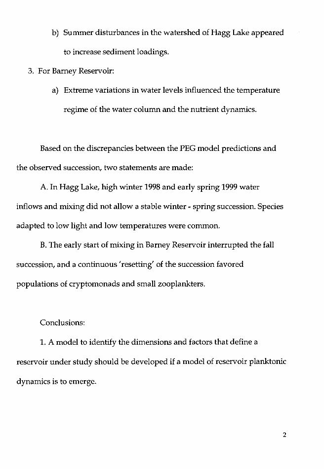
b) Summer disturbances in the watershed of Hagg Lake appeared
to increase sediment loadings.
3. For Barney Reservoir:
a) Extreme variations in water levels influenced the temperature
regime of the water column and the nutrient dynamics.
Based on the discrepancies between the PEG model predictions and
the observed succession, two statements are made:
A. In Hagg Lake, high winter 1998 and early spring 1999 water
inflows and mixing did not allow a stable winter - spring succession. Species
adapted to low light and low temperatures were common.
B. The early start of mixing in Barney Reservoir interrupted the fall
succession, and a continuous 'resetting' of the succession favored
populations of cryptomonads and small zooplankters.
Conclusions:
1. A model to identify the dimensions and factors that define a
reservoir under study should be developed if a model of reservoir planktonic
dynamics is to emerge.
2
2. The PEG model needs to be modified to include longitudinal
variations in the concentrations of nutrients and the effects of convective and
dispersive forces.
3. A hypothesis is put forth regarding the plankton dynamics should
fish stocking be initiated in Barney Reservoir: With fish exerting more
pressure on cyclopoids, calanoids will be able to colonize the reservoir; in
turn grazing-resistant algae, adapted to low nutrients, will become more
abundant.
3
THE DYNAMICS OF THE PLANKTONIC COMMUNITIES
OF TWO OREGON RESERVOIRS
by
MIGUEL ANGEL ESTRADA
A thesis submitted in partial fulfillment of the requirements for the degree of
MASTER OF SCIENCE in
BIOLOGY
Portland State University 2000

·B;asof lal{:i.owpuBl~ .Aw puB 'uoqda:mo::J lal{:J.OUI .Aw O.L
:uo!:J.B:>!paa

Acknowledgments:
I want to thank Dr. Richard R. Petersen, my advisor, for all his help. I
also want to acknowledge the help and advice of Dr. Yangdong Pan. Thanks
to Dr. Mark Sytsma for the corrections and ideas.
Advice on the methods for nutrient analysis and laboratory how-to
came generously from Kris Hueftle. The design of the field sampling also
took shape thanks to his advice, Thanks Kris.
Thanks to the personnel of the ESR office for their efforts to facilitate
the transportation to the reservoirs. Thanks to Karl Borg and the Forest
Grove Water Treatment Plan for the partial support to conduct this study.
Thanks to Kazuiro Sonoda for all his aid in the laboratory and in the
preparation of the defense of this thesis. Thanks to Paul Gill and Robert
Perkins, and to many other PSU students for their help. Thanks to Allen
Hamel, DEQ Oregon, for his help in creating the thermistor array.
Thanks to my wife Lydia for her support.
ii
TABLE OF CONTENTS
Dedication ................................................................................. i
Acknowledgements .................................................................... ii
LIST OF TABLES ........................................................................ vi
LIST OF FIGURES ..................................................................... vii
INTRODUCTION ....................................................................... 1
Reservoirs ........................................................................ 1
Models ............................................................................ 2
Assumptions .................................................................... 8
Focus and Purpose ............................................................ 9
MATERIALS AND METHODS .................................................... 10
Reservoirs ....................................................................... 10
Field methods .................................................................. 18
Laboratory Methods .......................................................... 23
Field Sampling Quality control. ............................................ 28
Laboratory quality control. .................................................. 30
RESULTS .................................................................................. 31
1. HAGG LAKE ......................................................................... 31
a) Physical Factors ............................................................. 31
b) Chemical factors ............................................................ 47
iii
c) Biological factors ............................................................ 70
2. BARNEY RESERVOIR. ............................................................. 86
a) Physical Factors ............................................................. 86
b) Chemical factors ............................................................ 102
c) Biological factors ............................................................ 124
SUMMARY ............................................................................... 139
Hagg Lake ....................................................................... 141
Barney Reservoir .............................................................. 144
DISCUSSION ............................................................................. 152
CONCLUSION ............................................................................ 157
REFERENCES ............................................................................. 17 4
APPENDIX A. LABORATORY PROCEDURES FOR WATER CHEMISTRY,
CATIONS AND CHLOROPHYLL-A ANALYSIS ............................... 179
Guidelines for the handling of samples (Jones, 1998): ................ 179
Laboratory Procedures: ...................................................... 180
Total Nitrogen: .................................................................. 182
Nitrate+ Nitrite Nitrogen: ..................................................... 183
Ammonium Nitrogen: ........................................................ 186
Total Phosphorus: .............................................................. 187
Soluble Reactive Phosphorus: .............................................. 189
Dissolved Silica .................................................................. 191 iv
Major Cations: Mg, Na, Ca and K .......................................... 193
Chlorophyll-a .................................................................... 194
APPENDIX B. PLANKTON COUNTING METHODS ....................... 197
v
LIST OF TABLES
Table 1. Reservoir and Watershed Data ............................................ 10
Table 2. Sampling dates, number of days between samples, and station
depths .......................................................................................... 1S
Table 3. Chemical analysis methods and calculation methods ................. 26
Table 4. Dominant Phytoplankton species in Hagg Lake (µm/ml) ............ 71
Table 5. Dominant Zooplankton species in Hagg Lake (µm/ml) .............. 76
Table 6. Dominant Phytoplankton species in Barney Reservoir (µm/ ml) ... 125
Table 7. Dominant Zooplankton species in Barney Reservoir (µm/ml) ..... 129
Table Sa. Descriptive statistics of Hagg Lake Data ................................ 163
Table Sa. Descriptive statistics of Hagg Lake Data (cont.) ...................... 164
Table Sb. Hagg Lake Epilimnetic Data ............................................... 165
Table 9a. Descriptive statistics of Barney Reservoir Data ........................ 16S
Table 9b. Barney Reservoir Epilimnetic Data ....................................... 170
Table 10. Anion Data from CCAL (Cameron Jones, 199S) ....................... 173
vi
LIST OF FIGURES
Figure 1. Reservoir Conceptual Model.. .............................................................. 6
Figure 2.General location of the reservoirs in the State of Oregon ................. 12
Figure 3.Hagg Lake and Barney Reservoir watersheds .................................... 12
Figure 4. Hagg Lake aerial picture (US Geological Service, 1990) .................. 15
Figure 5. Barney Reservoir aerial picture (US Geological Service, 1980) ....... 17
Figure 6. Hagg Lake. Water elevation and precipitation (data from TVID,
1999) .......................................................................................................................... 32
Figure 7. Water inflows and outflows in Hagg Lake (data from TVID,
1999) .......................................................................................................................... 33
Figure 8. Hagg Lake. Hydraulic Mean Residence Time (Years) ...................... 34
Figure 9. Hagg Lake. Water, Epilimnion, Secchi and Photic Zone Depths .... 35
Figure 10. Hagg Lake. Epilimnetic DO, Temperature and Chlorophyll-a ..... 37
Figure 11. Hagg Lake. Time-depth graph of Temperature (°C) ...................... 38
Figure 12. Hagg Lake. Temperature profiles from 9/15/1998 to
10/28/1998 .............................................................................................................. 39
Figure 13a. Hagg Lake. Time-depth graph of Dissolved Oxygen (mg/L) ... .41
Figure 13b. Hagg Lake. Time-depth graph of Dissolved Oxygen(% Sat) .... .42
Figure 14. Hagg Lake. Secchi and Photic depth ............................................... .43
Figure 15. Hagg Lake. Time-depth graph of Turbidity (NTU) ....................... .46
Figure 16. Hagg Lake. Time-depth graph of pH ............................................... .48 vii
Figure 17a. Hagg Lake. Time-depth graph of Conductivity (µS/ cm) ............ 50
Figure 17b. Hagg Lake. Conductivity profiles from July and October 1998 .51
Figure 18. Hagg Lake. Time-depth graph of Redox Potential (m V) ............... 53
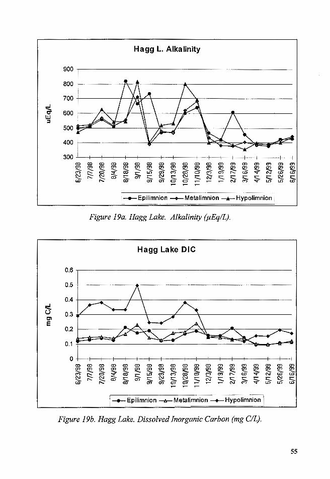
Figure 19a. Hagg Lake. Alkalinity (µEq/L) ....................................................... 55
Figure 19b. Hagg Lake. Dissolved Inorganic Carbon (mg C/L) ..................... 55
Figure 20. Hagg Lake. Chlorophyll-a (µg/l) ....................................................... 57
Figure 21. Hagg Lake. Epilimnetic Nitrogen species in µg/L ......................... 59
Figure 22. Hagg Lake. TP and Soluble Reactive Phosphorus in µg/L ........... 61
Figure 23. Hagg Lake. Silica(mg/l) and Bacillariophycea biovolumes .......... 62
Figure 24a. Hagg Lake. Cations: Na, K, Mg and Ca (mg/L) ............................ 65
Figure 24b. Hagg Lake. Anions: Cl and S04 (mg/L) ........................................ 65
Figure 25. Hagg Lake. Seasonal epilimnetic variations in Trophic State
Indices ...................................................................................................................... 67
Figure 26. Hagg Lake. TN:TP and Si:TP Nutrient Ratios ................................. 69
Figure 27. Hagg Lake. Dominant Phytoplankton Species ................................ 72
Figure 28. Hagg Lake. Total colonial vs. individual phytoplankton species. 74
Figure 29. Hagg Lake. Dominant Zooplankton Species ................................... 77
Figure 30. Hagg Lake. Predator vs. Non-predatory Zooplankton
Biovolumes .............................................................................................................. 78
Figure 31a. Hagg Lake. Calanoids and eucladocerans biovolumes ................ 79
Figure 31b. Hagg Lake. Dominant Rotifers and protozoans ............................ 80 viii
Figure 32a Hagg Lake. Shannon-Weiner Species Diversity Index .................. 84
Figure 32b Hagg Lake. Normalized (Diversity) Evenness ............................... 85
Figure 33. Barney Reservoir and its watershed. (USGS Maps) ........................ 87
Figure 34a. Barney R. Water elevation vs. precipitation, and storage versus
Releases .................................................................................................................... 89
Figure 34b. Barney Reservoir Hydraulic Mean Residence Time in Years ...... 90
Figure 35. Barney Reservoir. Epilimnion, Secchi and Photic depths ............. 91
Figure 36a. Barney Reservoir. Time-depth graph of Temperature (°C) ......... 93
Figure 36b. Barney Reservoir. Temperature profiles from July to September
1998 ........................................................................................................................... 94
Figure 37a. Barney Reservoir. Time-depth graph of Dissolved Oxygen
(mg/L) ...................................................................................................................... 96
Figure 37b. Barney R. Time-depth graph of Dissolved Oxygen(% Sat) ........ 97
Figure 38. Barney Reservoir. Secchi and Photic depth ...................................... 99
Figure 39. Barney Reservoir. Time-depth graph of Turbidity (NTU) .......... 101
Figure 40. Barney Reservoir. Time-depth graph of pH .................................. 104
Figure 41. Barney Reservoir. Time-depth graph of Conductivity (µS/ cm) 105
Figure 42. Barney Reservoir. Time-depth graph Redox Potential (m V) ...... 106
Figure 43a. Barney Reservoir. Alkalinity (µEq/L) .......................................... 108
Figure 43b. Barney Reservoir. Dissolved Inorganic Carbon (mg C/L) ....... 109
Figure 44. Barney Reservoir. Chlorophyll-a (µg/L) ....................................... 111 ix
Figure 45. Barney Reservoir. Total Nitrogen (µg N/L) .................................. 113
Figure 46. Barney Reservoir. Nitrate+nitrite and Ammonium (µg N/L) ... 113
Figure 47. Barney Reservoir. T P and SRP (µg P /L) ....................................... 115
Figure 48. Barney Reservoir. Silica (mg/L) ..................................................... 116
Figure 49. Barney Reservoir. Cations: Na, Ca, Mg and K (in mg/L) ........... 118
Figure 50. Barney Reservoir. Seasonal Trophic State Indices ........................ 121
Figure 51. Barney Reservoir. TN:TP and Si:TP Nutrient Ratios ................... 123
Figure 52. Barney Reservoir. Dominant Phytoplankton Species .................. 126
Figure 53. Barney Reservoir Total Colonial vs. Individual Species ............. 127
Figure 54. Barney Reservoir total biovolumes of phytoplankton and
zooplankton .......................................................................................................... 127
Figure 55. Barney Reservoir Dominant Zooplankton Species ...................... 130
Figure 56a. Barney Reservoir zooplankton, by feeding groups
(biovolumes) ......................................................................................................... 131
Figure 56b. Barney Reservoir Herbivore Zooplankton .................................. 132
Figure 57. Barney R. Total biovolumes of phytoplankton and herbivore
zooplankton .......................................................................................................... 134
Figure 58a. Barney Reservoir Shannon-Weiner Species Diversity Index .... 136
Figure 58b. Barney Reservoir Normalized (Diversity) Evenness ................. 138
Figure 59. The Plankton Ecology Group Model.. ............................................ 148
Figure 60a. Selected microphotographs of Hagg Lake phytoplankton ....... 149 x
Figure 60b. Selected microphotographs of Hagg Lake zooplankton ........... 150
Figure 61. Selected microphotographs of Barney R. Plankton ..................... 151
xi

INTRODUCTION
Reservoirs
Compared to natural lakes, man-made reservoirs are relatively new
features of the environment. The reasons for the existence of reservoirs are
utilitarian: to control floods, and to store water for irrigation etc. However,
the operation and management of a reservoir are not arbitrary; social and
physical or natural constraints regulate the range of their operations. Some
natural constraints on their operation include the finite amount of water
entering the reservoir and the storage capacity of the dam structure, and
social constraints manifest themselves as laws and operational procedures to
maintain a given water flow downstream, to maintain a suitable capacity in
reservoirs for drinking water and to avoid damage to the dam structure and
downstream areas.
The types and amounts of nutrients and sediment carried to the
reservoir by upland streams will reflect land use practices within the
watershed or drainage basin. Nutrients and sediment loadings will be the
governed by natural and social constraints, resulting in a reservoir that will
exhibit individual characteristics such as seasonal trophic and turbidity
levels. These attributes will change according to a yearly sequence of
meteorological events reflecting the climatic character of the larger
1
geographical area. At the local level, these events together with the action of
sedimentary and transport processes will have an impact on the biological
and physico-chemical dynamics that occur within the reservoir (Thornton et
al., 1990).
Limnological studies of reservoirs are time consuming and difficult to
conduct owing to their "lake-river" nature (Thornton et al., 1990). Ryder
(1978) described reservoirs as a distinct category of ecosystems retaining the
characteristics of lotic and lentic environments. This hybrid nature is
exemplified by the coexistence and overlap of many processes that
characterize rivers and lakes. Transport and sedimentary processes create
distinct riverine, transitional and lacustrine zones, and material gradients
that extend from headwaters to dam structures (Thornton et al., 1990). The
effect of these processes is felt throughout the length of reservoirs and take
the form of pulses of nutrients and suspended materials (Thornton et al.,
1990).
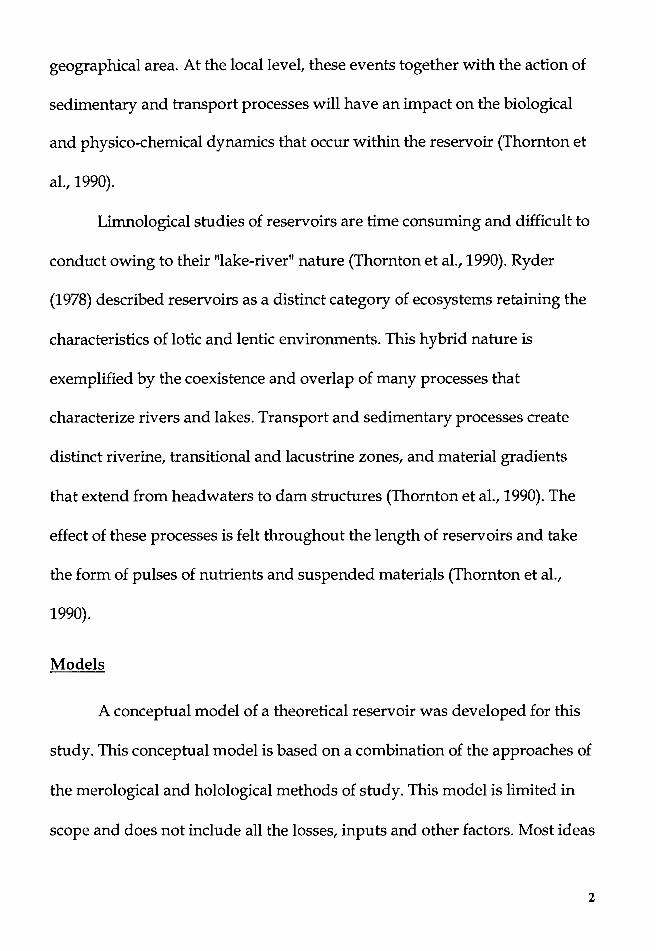
Models
A conceptual model of a theoretical reservoir was developed for this
study. This conceptual model is based on a combination of the approaches of
the merological and holological methods of study. This model is limited in
scope and does not include all the losses, inputs and other factors. Most ideas
2
and relationships used to create this model originated from Thornton et al.
(1990).
There are various theoretical models that deal directly or indirectly
with the plankton dynamics. Tilman (1982) proposed an equilibrium theory
of competition for limiting resources (consumer-resource theory), and tried
to explain the role of competition in the emergence of diver_sity. This theory
was not applied to this study because the data obtained was from non
manipulated, non-experimental fieldwork. Reynolds (1996) proposed a
demographic approach (CS R model) to interpret the interactions of the
phytoplankton. However, Reynolds (1996) approach could not be applied to
this study, as it still does not incorporates the zooplankton dynamics or
defines the place of predation in his model. The PEG (Sommer et al. 1986)
model summarizes the plankton succession in a 'generic' lake through
twenty-four verbal statements. Because these statements depict a generalized
phytoplankton- herbivorous zooplankton dynamics, they were tested on
how well they explained the plankton dynamics in the lacustrine zone of a
reservoir.
Thus, for this study, the PEG and the conceptual models were used as
the basis to understand the dynamics of the abiotic and the biotic elements
and to test its suitability in explaining the plankton dynamics of reservoirs.
3
Conceptua!Afodel
In developing this conceptual model, it was assumed that the coarse
scale factors such as land use practices, watershed geomorphology, the
meteorology and climate of the area are the components that give a
reservoirs its initial character (Thornton et al., 1990).
In this conceptual model, the transport and sedimentary processes are
affected by the residence times and the amount and kinds of inflows and
outflows. These processes help define the extent of the longitudinal zonation
(riverine, transitional and lacustrine zones) and gradients of dissolved matter
(Thornton et al., 1990). For example, extremely short residence times would
eliminate pelagic phytoplankton by causing cell washout rates greater than
phytoplankton reproduction rates (Thornton et al., 1990). Wind mixing
interactions will depend on water elevation (or depth), basin shape and
shoreline development, and will affect the dilution and settling of sediments
and nutrients entering through the inflows. Turbidity, particulate matter and
nutrient availability will interact with the physical processes described above
and impact the standing crop of phytoplankton (Thornton et al., 1990). The
phytoplankton (and bacteria) in turn will start the trophic chain by
supporting herbivorous zooplankton, predatory zooplankton, insects,
planktivorous fish and other vertebrates.
4
Although the dynamics and characteristics of reservoirs appears
complex and difficult to study, this appearance vanishes as soon as one
realizes that a methodical approach, coupled with some awareness of the
interacting factors that make a reservoir, can be used to partition or select
one particular dimension or problem of interest. Once this dimension is
selected, the elements left out can still be referenced to aid in explaining the
changes observed. The conceptual model developed here served to identify
some of the many dimensions and factors that define a theoretical reservoir.
The dimension of interest chosen for this study was the dynamics of the
planktonic successions from the June 1998 to early July 1999, and the place
that these successions occupy within the interacting components that make
up Hagg Lake and Barney Reservoir (Figure 1 ).
The Plankton Ecology Group (PEG) Model
The PEG (Sommer et al. 1986) model is composed of 24 verbal
statements. Statements 1to5 describe the planktonic spring succession and is
summarized as follows: increases in light and availability of nutrients
permits the growth of small centric diatoms and cryptomonads which in turn
support the growth of large herbivorous zooplankton until their grazing
pressure on phytoplankton is such that their elimination creates a period or
phase of 'clear water'.
5

O'I
Conceptual Model of the Plankton Dynamics in a Reservoir
Arrows indicate interactions or relationships.
Xi-Zi = Arbitrary Location along the main Longitudinal axis of the reservoir.
**Not all losses and Inputs are included**
Land Use..__ __
Meteorology
Inflow of Waters with sediments and Nutrients
Longitudinal Zonation and formation of
Concentration Gradients
Particulate Matter
Losses to Outflows
Underflow/Overflow of Waters 1 )I
with sediments and Nutrients
Transport and Sedimentary Processes
Outflows (at variable
depths)
Synoptic Cycles I ~ >I Wind Mixing Residence time I{ •
Figure 1. Reservoir Conceptual Model.
The statements 6 to 16 of the PEG model describe the summer
planktonic succession and are summarized as follows: decreases in herbivore
zooplankton due to food limitation and low fecundity and fish predation
allow the phytoplankton populations to bounce back, so that phosphorus is
almost depleted, and the small zooplankton populations begin to increase.
The two groups decrease as nutrients are consumed. Dinoflagelates or
Cyanophytes begin to dominate the phytoplankton and are replaced later by
nitrogen fixing Cyanophytes if nitrogen is depleted. At this point in late
summer, large bodied zooplankton gives way to smaller zooplankton. The
herbivore zooplankton attains high diversity by partitioning the available
food supply. Temperature affects the zooplankton composition and its
fluctuations.
The statements 17 to 20 of the PEG model describe the fall planktonic
succession and are summarized as follows: physical changes caused by the
overturn or mixing of the water column favor species adapted to low light
and continuous mixing disturbance and low fish predation favors big-bodied
zooplankton. The statements 21 to 24 of the PEG model describe the winter
planktonic succession and are summarized as follows: low light and its
consequence the low algal biomass combined with low temperatures signals
the start of the diapause period in some zooplankton or lowers the fecundity
in another zooplankton species.
7
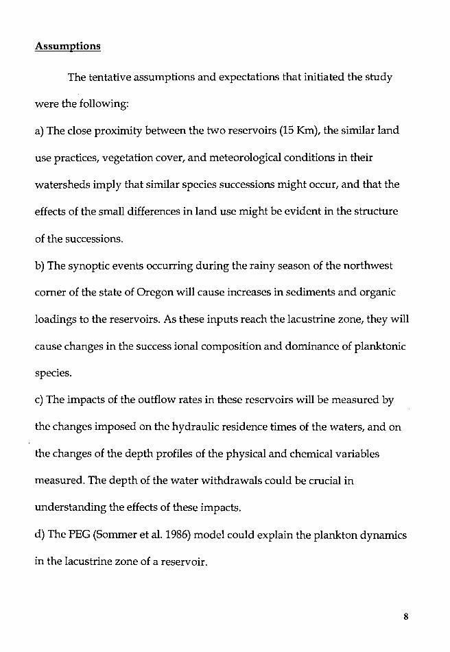
Assumptions
The tentative assumptions and expectations that initiated the study
were the following:
a) The close proximity between the two reservoirs (15 Km), the similar land
use practices, vegetation cover, and meteorological conditions in their
watersheds imply that similar species successions might occur, and that the
effects of the small differences in land use might be evident in the structure
of the successions.
b) The synoptic events occurring during the rainy season of the northwest
corner of the state of Oregon will cause increases in sediments and organic
loadings to the reservoirs. As these inputs reach the lacustrine zone, they will
cause changes in the success ional composition and dominance of planktonic
species.
c) The impacts of the outflow rates in these reservoirs will be measured by
the changes imposed on the hydraulic residence times of the waters, and on
the changes of the depth profiles of the physical and chemical variables
measured. The depth of the water withdrawals could be crucial in
understanding the effects of these impacts.
d) The PEG (Sommer et al. 1986) model could explain the plankton dynamics
in the lacustrine zone of a reservoir.
8
Focus and Purpose
This study focuses on the lacustrine zone of Hagg Lake and Barney
Reservoir, particularly on the epilimnetic layer, at 1 m below the water
surface at the sampling stations. Other samples were taken at the
metalimnion (thermocline) and the hypolimnion depths, and profiles were
created from measurements at different depths of temperature, dissolved
oxygen, pH, turbidity and conductivity. The plankton studied in this thesis
includes only microscopic algae and microscopic zooplankton living in the
pelagic zone.
The purpose of the study was to identify the succession dynamics of
the planktonic species in the reservoirs, and test the suitability of the PEG
model to explore the relationships between these successions and the
physical and chemical variables measured from June 1998 to July 1999.
9
MATERIALS AND METHODS
This section summarizes reservoir data, field sampling and the
laboratory analysis methods. Detailed laboratory analytical procedures for
water chemistry and chlorophyll-a are given in Appendix A. The
phytoplankton and zooplankton sampling and counting procedures are
given in Appendix B.
Reservoirs
The reservoirs studied were Hagg Lake and Barney Reservoirs. These
two reservoirs are located in the northwest corner of the State of Oregon
(Figure 2).
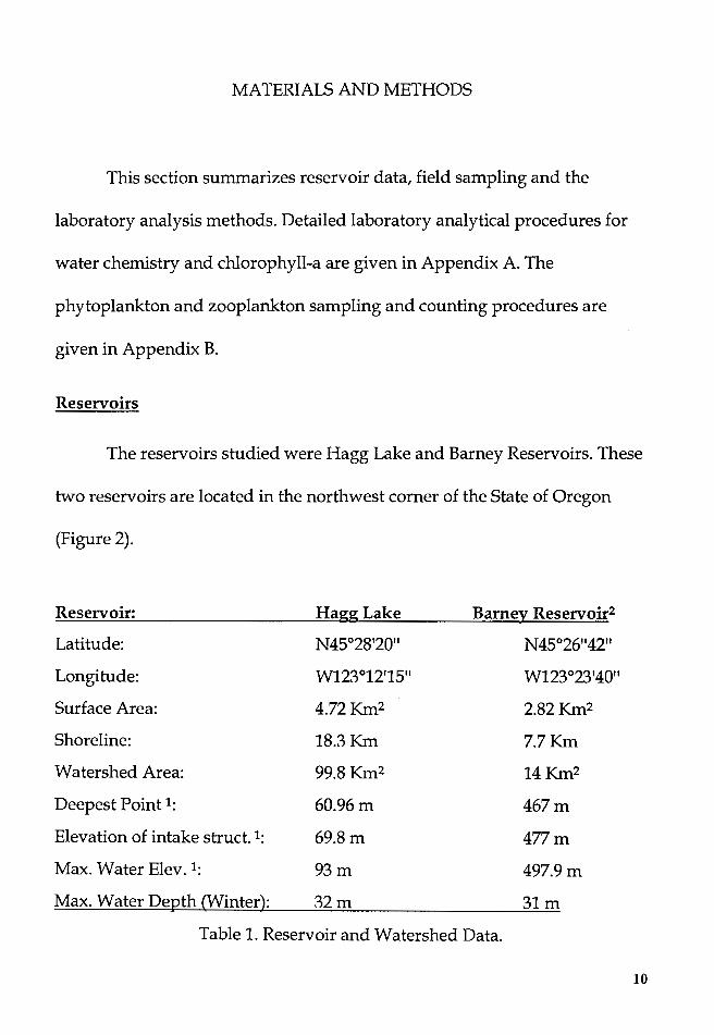
Reservoir: Hagg Lake Barney Reservoir2
Latitude: N45°28'20" N45°26"42"
Longitude: W123°12'15" w123°23'40"
Surface Area: 4.72Km2 2.82Km2
Shoreline: 18.3Km 7.7Km
Watershed Area: 99.8 Km2 14Km2
Deepest Point 1: 60.96 m 467m
Elevation of intake struct. 1: 69.Sm 477m
Max. Water Elev. 1: 93m 497.9m
Max. Water Depth (Winter): 32m 31m
Table 1. Reservoir and Watershed Data.
10
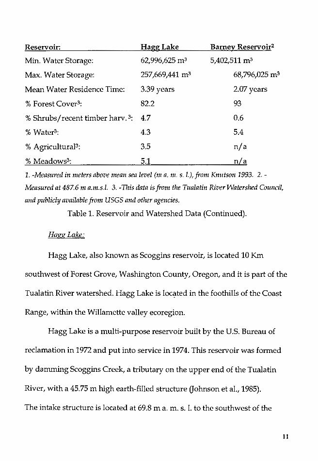
Reservoir: Hagg Lake Barney Reservoir2
Min. Water Storage: 62,996,625 m3 5,402,511 m3
Max. Water Storage: 257,669,441 m3 68,796,025 m3
Mean Water Residence Time: 3.39 years 2.07 years
% Forest Cover3: 82.2 93
% Shrubs/ recent timber harv. 3: 4.7 0.6
% Water3: 4.3 5.4
% Agricultural3: 3.5 n/a
% Meadows3; 5.1 nLa 1. -Measured in meters above mean sea level (ma. m. s. l.), from Knutson 1993. 2. -
Measured at 487.6 m a.m.s.l. 3. -This data is from the Tualatin River Watershed Council,
and publicly available from uses and other agencies.
Table 1. Reservoir and Watershed Data (Continued).
Hagg Lake:
Hagg Lake, also known as Scoggins reservoir, is located 10 Km
southwest of Forest Grove, Washington County, Oregon, and it is part of the
Tualatin River watershed. Hagg Lake is loc~ted in the foothills of the Coast
Range, within the Willamette valley ecoregion.
Hagg Lake is a multi-purpose reservoir built by the U.S. Bureau of
reclamation in 1972 and put into service in 1974. This reservoir was formed
by damming Scoggins Creek, a tributary on the upper end of the Tualatin
River, with a 45.75 m high earth-filled structure Gohnson et al., 1985).
The intake structure is located at 69.8 ma. m. s. l. to the southwest of the
11

ii fl 0
~ .. ll.
[I]
State of Oregon, U.S.A.
Figure 2. General location of the reservoirs in the State of Oregon.
~ N
River
Figure 3.Hagg Lake and Barney Reservoir watersheds.
12
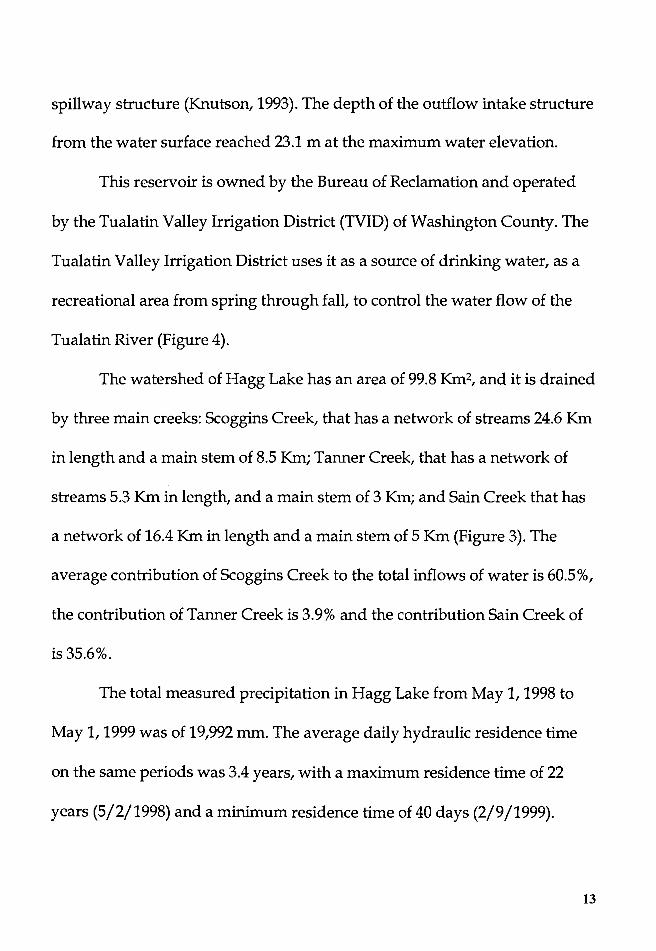
spillway structure (Knutson, 1993). The depth of the outflow intake structure
from the water surface reached 23.1 mat the maximum water elevation.
This reservoir is owned by the Bureau of Reclamation and operated
by the Tualatin Valley Irrigation District (TVID) of Washington County. The
Tualatin Valley Irrigation District uses it as a source of drinking water, as a
recreational area from spring through fall, to control the water flow of the
Tualatin River (Figure 4).
The watershed of Hagg Lake has an area of 99.8 Krn2, and it is drained
by three main creeks: Scoggins Creek, that has a network of streams 24.6 Km
in length and a main stem of 8.5 Km; Tanner Creek, that has a network of
streams 5.3 Km in length, and a main stem of 3 Km; and Sain Creek that has
a network of 16.4 Km in length and a main stem of 5 Km (Figure 3). The
average contribution of Scoggins Creek to the total inflows of water is 60.5%,
the contribution of Tanner Creek is 3.9% and the contribution Sain Creek of
is 35.6%.
The total measured precipitation in Hagg Lake from May 1, 1998 to
May 1, 1999 was of 19,992 mm. The average daily hydraulic residence time
on the same periods was 3.4 years, with a maximum residence time of 22
years (5/2/1998) and a minimum residence time of 40 days (2/9/1999).
13

This reservoir has a maximum storage capacity of 257,669,441 m3 of
water. The pool is lowered during the dry summer months by an average of
6.7 m, and filled during the winter months. The drainage basin covers an
area of 99.8 Km2 (Figure 2).
The watershed is covered mostly by thick soils of clay and silt
overlying bedrock that is a mixture of sandstone and older volcanic rocks
(Johnson et al., 1985). The forest vegetation of the watershed is composed of
western hemlock and Douglas fir (Pseodotsuga menziesii, Tsuga heterophylla)
that covers approximately 82.2%. Mountain snowberry (Symphoricarpus sp.)
and Mountain sagebrush (Artemisia sp.) cover approximately 4.7% of the
watershed. Timber harvesting and livestock grazing and other agricultural
activities take place in the watershed.
Barney Reservoir
J.W. Barney Reservoir is located 24 Km southwest of Forest Grove,
Washington County, Oregon (Figure 3), and 14.9 Km from Hagg Lake. It is in
the North fork of the Trask River, and it is part of the Trask River watershed
of the Coast Range. The watershed of Barney Reservoir neighbors the
Tualatin River watershed and straddles Washington and Yamhill Counties.
An aqueduct is used to transfer water from Barney Reservoir to the Tualatin
River. Initial construction of this reservoir was finished 1970 with an original
capacity of 16,187,300 m3. In December 1977, the height of
14

45N 29' 56' 5,038,400.(1
45N 21' 12'' 5,035,200.0
123W 15' 22"" 480 1000,I
45N 27' 20" s,o:n,100.0 ,_-
121w 1s• 2100
410,0IO.O
Hagg Lake (Scoggins Reservoir) Photo courtesy of the US Geological Survey.
Image found at: http1/www.tenaserver.microsoftcomt
123W 14' 01" 481,601.0
123w 14" or 411,HO.I
l23W 12' 54" 413,211.1
123W 12' 5 .... 4U,200.I
129:W 11' 41" 45N 30' 48"' 414,110,0 5,040,00D.I
-~!fil'JilO !tWJ i '&!\',,.~
123W 11' 40" 414,HO.O
5N 2t' 56" 031,400.0
5,035,200.0
45N 27 21" 5,0U,600,0 123W 10' 26"' 416,400.0
Figure 4. Hagg Lake aerial picture (US geological Service, 1990)
15
I
the dam was increased (Karl Borg, Forest Grove Treatment Plant, personal
communication) and the additional improvements were completed in 1999.
By March 1999 it was able to hold 4.25 times the original volume (68,796,025
m3). This reservoir is used for stream flow control, and as a supplementary
water source by the TVID (Figure 5).
The watershed of Barney Reservoir is fed by the upper 5 Km of the
North fork of the Trask River and its 3.8 Km of shorter streams; the rest of
the drainage network includes several smaller and intermittent streams. The
drainage basin of Barney Reservoir covers an area of 14 Km2. The watershed I
is largely covered by clay and silt soils over bedrock that is a mixture of
tuffaceous sedimentary rocks and tuff (Walker and MacLeod, 1991).
The forest vegetation of the watershed is composed of western
hemlock and Douglas fir (Pseodotsuga menziesii, Tsuga heterophylla) and it
covers approximately 93 % of the watershed. Human activities on the
watershed of Barney Reservoir include timber harvesting and off-road
vehicles recreation.
It is also important to note that due to recent increases in the storage
capacity of the dam, the area covered by water, and the water depth and
surface elevation also increased. Also, that during the study period, some of
the roots and other organic debris from the vegetation that covered the
inundated areas still remained on the ground.
16
Barney Reservoir, Washington Co. 55 km W of Portland, Oreqon, United States
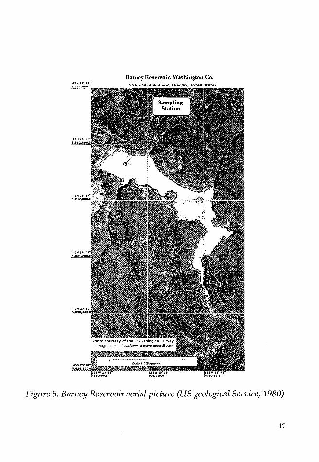
Figure 5. Barney Reservoir aerial picture (US geological Service, 1980)
17
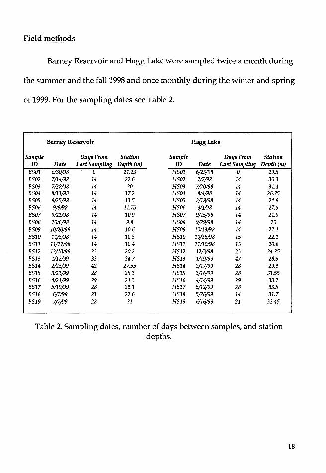
Field methods
Barney Reservoir and Hagg Lake were sampled twice a month during
the summer and the fall 1998 and once monthly during the winter and spring
of 1999. For the sampling dates see Table 2.
Barney Reservoir Hagg Lake
Sample Days From Station Sample Days From Station ID Date Last Sampling Depth (m) ID Date Last Sampling Depth (m)
8501 6/30/98 0 21.23 H501 6/23/98 0 29.5 8502 7/14/98 14 22.6 H502 7/7/98 14 30.3 8503 7,128/98 14 20 H503 7,120/98 14 31.4 8504 8/11/98 14 17.2 H504 8/4/98 14 26.75 8505 8,125/98 14 13.5 H505 8/18/98 14 24.8 8506 9/8/98 14 11.75 H506 9/1/98 14 27.5 8507 9,122/98 14 10.9 H507 9/15/98 14 21.9 8508 10/6/98 14 9.8 H508 9/29/98 14 20 8509 10,120/98 14 10.6 H509 10/13/98 14 22.1 8510 11/3/98 14 10.3 H510 10/28/98 15 22.1 8511 11/17/98 14 10.4 H511 11/10/98 13 20.8 8512 12/10/98 23 20.2 H512 12/3/98 23 24.25 8513 1/12/99 33 24.7 H513 1/19/99 47 28.5 8514 2;23/99 42 27.55 H514 2/17/99 28 29.3 8515 3,123/99 28 25.3 H515 3/16/99 28 31.55 8516 4/21/99 29 21.3 H516 4/14/99 29 33.2 8517 5/19/99 28 23.1 H517 5/12/99 28 33.5 8518 6/7/99 21 22.6 H518 5/26/99 14 31.7 8519 7/7/99 28 21 H519 6/16/99 21 32.45
Table 2. Sampling dates, number of days between samples, and station depths.
18
Main station. depth and water levels
The main stations for both reservoirs were located at least 300 m away
from their respective dam structures, and where reservoirs were deepest.
The station locations were chosen so as to locate the sampling station in the
lacustrine zone of the reservoirs. The depths were measured with a small
depth sounder (Humminbird®, Wide Vision). The water elevation in Barney
Reservoir was measured by reading the water elevation markers of the dam;
the water elevation from Hagg Lake was obtained from the official daily
measurements taken by the personnel in charge of the dam operations.
Secchi depth and irradiance
The Secchi depth was measured with a Secchi disk of 20 cm in diameter. The
light intensity, in µEinsteins m-2 ·s-1, was measured with a LICOR® spherical
underwater sensor (No. SPQA 0275) that measured the photosynthetic active
radiation (PAR). This sensor was connected by a cable to a LI-1000® data
logger (LDL 2500). The rates of light extinction and the limits of the photic
zone (depth where the light intensity measures 1 % of the incoming light at
19
the surface) were calculated from these measurements (Wetzel and Likens,
1991).
DO. turbidity. conductivity. temperature and pH
A temperature array or string of Vemco® (Minilog®) temperature monitors
was built by attaching 31 Vemco® units to an aircraft cable 30 m long. After
each trip, the temperature data were downloaded from the units through a
Vemco® optical computer interface.
Other physical and chemical variables were measured with a
Hydrolab® H20 multiprobe (SN25373) attached by a 25-meter cable to an
SVR3-DL Surveyor3® data logger (SN25371). Readings were taken at 0.1 m,
0.5 m and then 1 m intervals until reaching the bottom of the reservoir or
reaching 24.5 m. For these variables a reservoir profile was created. The
variables measured with the Hydrolab® H20 multiprobe were:
Temperature (degrees Celsius).
Dissolved oxygen (mg/L).
Conductivity (µS/ cm).
Turbidity (NTU units).
pH units.
20

Missing values (to 0.2 m above the bottom), were interpolated using
the temperature data from the array or string of Vemcos® as a reference for
the rates of change in the very few cases when the depth of the reservoirs
was greater than 24.5 m.
Water samples for chlorophyll-a, nutrient analysis and alkalinity
Water samples were from the epilimnion (1 m below the water
surface), the metalimnion (most likely point of the thermocline defined by
the temperature profile measured by the Hydrolab® unit), and the
hypolimnion (1 m above the bottom of the reservoirs). The metalimnion
sample was taken whenever there was a thermocline (or more than sixty
percent of the cases).
Water samples were collected with a vertical 3-liter Van Dorn bottle
(Scott Instruments Inc.). The water samples were placed in 250 ml Nalgene®
bottles. These bottles had been acid soaked in the laboratory in a 4 %
hydrochloric acid bath (for at least 12 hours) and rinsed eight times with
ultra pure deionized water.
For each sample, a 250 ml dark high-density polyethylene (HDPE)
Nalgene® bottle and four 250 ml clear HDPE Nalgene® bottles were used. In
the field, the HDPE bottles were rinsed with reservoir water at least twice,
21
and then filled with water from the Van Dorn unit. The bottles were then
placed in a cooler with ice.
Upon returning to shore, the sample in the dark bottle was filtered
with a Nalgene® hand pump filtration set up and a glass microfiber filter
(Whatman® GF /F 47 mm). These filters were washed with deionized water
and oven dried at 55° C. for at least 48 hours. Filtration was always within
two hours after sampling. The filtered sample was stored in a clean clear
HDPE Nalgene® bottle for chemical analysis. Three drops of saturated
MgC03 were added to the filter, it was placed in a filter holder, wrapped in
foil and placed in ice to be analyzed for chlorophyll-a.
Samples from the epilimnion, metalimnion and hypolimnion were
analyzed for alkalinity. Alkalinity was measured in mg/L of CaC03 in the
field, and in and µEq/L in the laboratory. The field method used was that of
titration with color indicators (bromcresol green-methyl red and
phenolphthalein). The laboratory method was the Gran titration (Wetzel and
Likens, 1991). Dissolved inorganic carbon in mg C/L was derived from pH
and Alkalinity data following the procedure described in Wetzel and Likens,
(1991).
22
Phytoplankton and zooplankton samples
Water samples for phytoplankton analysis were collected with the
Van Dorn bottle. 2.5 ml of Lugol's solution was added to the 250 ml HDPE
bottles marked for the phytoplankton samples to reach a 1 % final
concentration of Lugol's fixative. Once in the laboratory, the samples were
stored in the dark, in a refrigerated room at 4 ° C.
The zooplankton samples were collected with a folding plankton net
of a diameter of 49 cm. Depending on the amount of water in the sample,
from 1to3 ml of formalin (40% formaldehyde buffered with sodium acetate
(Wetzel and Likens, 1991)), were added to preserve the organisms. Once in
the laboratory, the samples were stored in the dark, in a refrigerated room at
40 c.
Laboratory Methods
Three of the 38 sets collected were submitted to the Cooperative
Chemical Analytical Laboratory (CCAL) in Corvallis, Oregon for nutrient
and major ion analysis. The CCAL is a laboratory established by the USDA
Forest Service and the Department of Forest Science, Oregon State
University. These samples are marked with an asterisk in the tables where
they are included. The rest of samples were analyzed at Portland State
University by the author.
23

Chemical analysis methods and calculation methods
Concentration of the following analytes were measured: total
nitrogen, nitrate+nitrite, ammonium, total phosphorus, soluble reactive
phosphorus, dissolved silica, dissolved magnesium, dissolved sodium,
dissolved calcium and dissolved potassium. The units of measurement were
µg/L, except in the case of silica and the cations that were measured in
mg/L. The samples were frozen as soon after they were collected, and
thawed before the analysis; the handling of the samples followed the
guidelines described in the AHPA, 1988, as modified in the CCAL
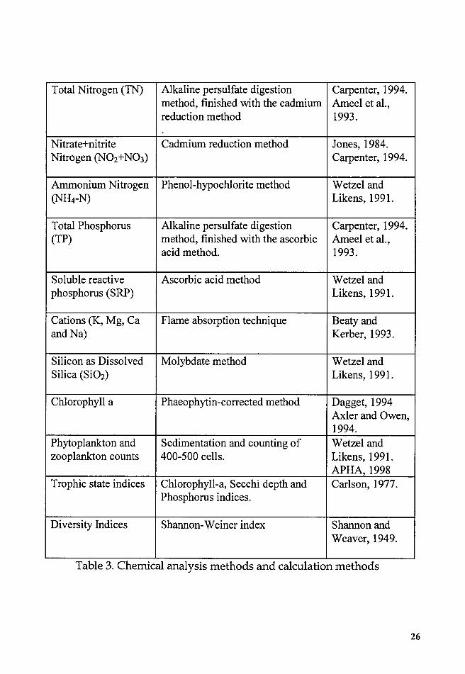
Guidelines Gones, 1998). Table 3 describes the Chemical analysis methods
and calculation methods used.
Trophic State Index ([SJ)
The trophic state indices proposed by Carlson (1977) were used here
to classify Hagg Lake and Barney Reservoir. According to Carlson (1977) and
Johnson (1985), oligotrophic lakes fall within the range of 20 to 35 TSI units,
mesotrophic lakes in the range of 35 to 50 TSI units, and eutrophic lakes in
the range of 51 to 65 TSI units, with the biomass doubling every 10 TSI units.
24
Plankton counting and identification
Dominant organisms were identified to species, and the rest to genus.
A minimum of 400-500 cells was counted from each sample using a
Nannoplankton (phytoplankton) and a Sedgwick-Rafter cell (Zooplankton).
25
Total Nitrogen (TN) Alkaline persulfate digestion Carpenter, 1994. method, finished with the cadmium Ameel et al., reduction method 1993.
Nitrate+nitrite Cadmium reduction method Jones, 1984. Nitrogen (N02+N03) Carpenter, 1994.
Ammonium Nitrogen Phenol-hypochlorite method Wetzel and (Nlli-N) Likens, 1991.
Total Phosphorus Alkaline persulfate digestion Carpenter, 1994. (TP) method, finished with the ascorbic Ameel et al.,
acid method. 1993.
Soluble reactive Ascorbic acid method Wetzel and phosphorus (SRP) Likens, 1991.
Cations (K, Mg, Ca Flame absorption technique Beaty and and Na) Kerber, 1993.
Silicon as Dissolved Molybdate method Wetzel and Silica (Si02) Likens, 1991.
Chlorophyll a Phaeophytin-corrected method Dagget, 1994 Axler and Owen, 1994.
Phytoplankton and Sedimentation and counting of Wetzel and zooplankton counts 400-500 cells. Likens, 1991.
APHA, 1998 Trophic state indices Chlorophyll-a, Secchi depth and Carlson, 1977.
Phosphorus indices.
Diversity Indices Shannon-Weiner index Shannon and Weaver, 1949.
Table 3. Chemical analysis methods and calculation methods
26
Phytoplankton counting and identification:
Cell were counted and measured to calculate their approximate
biovolumes based on simple geometric formulae (Wetzel and Likens, 1991).
Cell volumes (biovolumes) were used to achieve a better evaluation of the
cellular biomass of the species present in the samples and their importance in
the successions (Wetzel and Likens, 1991). The sources for the identification
of diatoms were Vinyard (1979), Weber (1971), Patrick and Reimer (1966) and
Krammer and Lange-Bertalot (1991). The sources for the identification of the
other algae were West and West (1971), Prescott (1962), Prescott (1978),
Lewis and Britton, (1971), Patrick and Reimer (1966), Huber-Pestalotz (1941),
Smith (1950) and Contant and Duthie (1978).
Zooplankton counting and identification:
Individuals were counted and measured. The average calculated
biovolume were compared to published biovolumes, and in some cases
biovolumes from the literature were used to calculate the final average
biovolume per species (Wetzel and Likens, 1991), (Nauwerck, 1963). The
sources for the identification of zooplankton were Corliss, (1979), Sternberger
(1979), Torke, (1974), Thorp and Covich Ed. (1991) and Pennak (1989).
27

Field Sampling Quality control
Bottles
Bottles were placed in a 4 % hydrochloric acid bath for at least 6 hours.
After rinsing the bottles with deionized water they were set to dry. Once
dried, they were tightly closed until the moment when the samples were
collected. The bottles were rinsed with reservoir water at least twice before
the water collected with the Van Dorn Bottle or plankton net was added to
them. Bottle labels were checked during filling. Sample bottles were placed
in a cooler filled with ice for transport to the laboratory. In the laboratory,
the samples for nutrient analysis were kept in a freezer until analysis. The
other samples were stored in the dark in a refrigerated room at 4 ° C.
Labeling
A set of sampling conventions was developed, and adhered to, during
the study period. Labels were made and placed on outside of the bottles used
for the sampling.
Field Notes
Sampling date, time, weather conditions, Secchi disk depth, irradiance
data, main station depth, field trip problems and other information were
recorded on rainproof paper. The temperature profiles were created using
28
these notes to identify the thermocline and the plankton net ranges. The data
from these notes were used to create electronic files.
Field Instruments
All instruments and tools were cleaned before and after each field
trip. Batteries were replaced or recharged as needed. Before and after each
trip, the Hydrolab® unit was calibrated against laboratory standards,
following the calibration guidelines described in the manual of the unit. The
Vemco® units were dried, cleaned; the data was downloaded through the
computer interface, and were re-programmed for the next trip.
Replicates and handling of samples
Replicates samples were taken whenever it was possible (65.7 % of the
time). Of the 38 sampling sets from both Barney Reservoir and Hagg Lake, 25
of these had replicates. Nutrient analysis, chlorophyll-a, ion and alkalinity
analysis were performed for all of the replicates. The plankton counts of
replicates were as follows: 20 phytoplankton counts were from replicate
samples (65.7% ), and 4 zooplankton counts were from replicate samples
(10.5%). Three of the 38 sampling sets (7.9%) were sent to be analyzed for
nutrients and ions to the CCA Laboratory, in Corvallis, Oregon.
29
Laboratory quality control
The main procedures followed to ensure accurate results were: a) the
systematic cleaning of equipment and glassware and, b) the careful handling
and measuring of the different chemical components. The glassware,
reusable tips of micropipettes and stirrer bars were acid washed in
accordance with the steps described above. The guidelines in the manual of
the instruments were heeded and the chemical recipes were strictly followed
(Appendix A). All the water samples and replicates were analyzed.
30

RESULTS
1.HAGGLAKE
In this section the physical, chemical and biological factors that were
measured during the sampling period are described and analyzed. Table 8a
and 8b list a summary of descriptive statistics for Hagg Lake data.
Microphotographs of selected specimens of the plankton are presented in
figures 60a and 60b.
a) Physical Factors
1. Water Inflow and Outflows
The data on the water inflows and outflows in Hagg Lake came from
monthly dam operations reports prepared for the Tualatin Valley Irrigation
District (TVID) by the current dam operator, Wally Otto.
In Hagg Lake the inflow and outflow regime during the study period
can be described as follows: From June to November, when most of the
weather fronts were less severe or moved to higher latitudes, the releases of
water were greater than the inflows, and the water level began to drop from
92 m above mean sea level (a.m.s.l.) to a low of 80 m a.m.s.l. (Figure 6).
During the month of November the inflows exceeded outflow, and
the water levels rose from a low of 80 m a.m.s.1. to around 86 m a.m.s.l. From
31
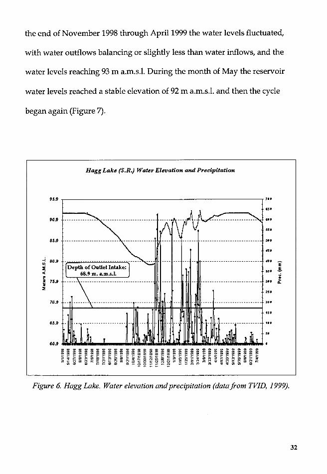
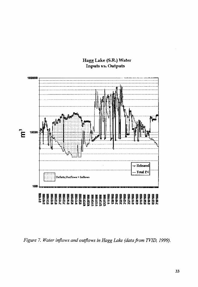
the end of November 1998 through April 1999 the water levels fluctuated,
with water outflows balancing or slightly less than water inflows, and the
water levels reaching 93 m a.m.s.l. During the month of May the reservoir
water levels reached a stable elevation of 92 m a.m.s.l. and then the cycle
began again (Figure 7).
_j ui ~ .r. ~
Hagg Lake (S.R.) Water Elevation and Precipitation
95.9 7 ..
cs•
, .. ss•
SU
4Sf
80.9 - - - - .. - - - ·- - - .. - - _.....,_ - - - -- - - - - - - - --- - -- - - - - - - - _.. 40• E Depth of Outlet Intake:
68.9 m. a.m.s.I. 3Sf .§.
.;
~ 75.9 -- .. 1-11-------------------------- ...... l•• ~ • :E 25'
70.9 ~- - •• - - - - - - -~ - - - - - - - - - - -- - - - - - - ·- - - - - - - - .......... , _____ _. __ -- ------ ------- ___ _.. 20•
1s•
65.9 ~- ···- --- - -- ------ ----- - ----·--~·· -----~- 1U
Sf
60.9 MM .. Jl.lillila els:::: ::adl111l1~iH111t\1Mi111Mi1:G11.iti1.iW11llult::Mil!Jil't II lail d m m m m m m m m m m m m m m m m m m m m m m m m m m m m m m m m m m m m m m m m m m m m m m m m m m m
~ E ~ ~ S ~ ~ i ~ ~ a ~ ~ i ~ ~ ~ ~ ~ ~ ~ ~ ~ a ~ ~ a a ~ ~ ~ ~ ~ s - - -- -
m m m m m m m m m m m m m m m m m m m m m m m m m m m m m m m m m m m m S ~ ~ ~ 5 E a ~ ~ i S 5 ~ ~ M ~ ~ ~ ~ ~ ~ ~ ~ ~
Figure 6. Hagg Lake. Water elevation and precipitation (datafrom TVID, 1999).
32
~
E
Hagg Lake (S.R.) Water Inputs vs. Outputs
10000000~~~~~~~~~~~~~~~~~~~~~~~~~~~
M"1ttr·111nwa-wi-.ir- - - - - - -- - - - - - --- - - -- - - - - - -
100000
"T" -----l~~:.::::::=:-----------------------------1~::;i UH
100) biiliMllMllllAIMllMMiiillllllllMllllliilM&MllllMlllWlaHMllllMllWIWlllllllUllMllHIWWlllMllMllHllliihiiiliWllWIWIM.
111111111111111111111111111111 ~~~~~~~~~~~~;g~g~~~~~~~t~~~~~~
Figure 7. Water inflows and outflows in Hagg Lake (data.from TVID, 1999).
33
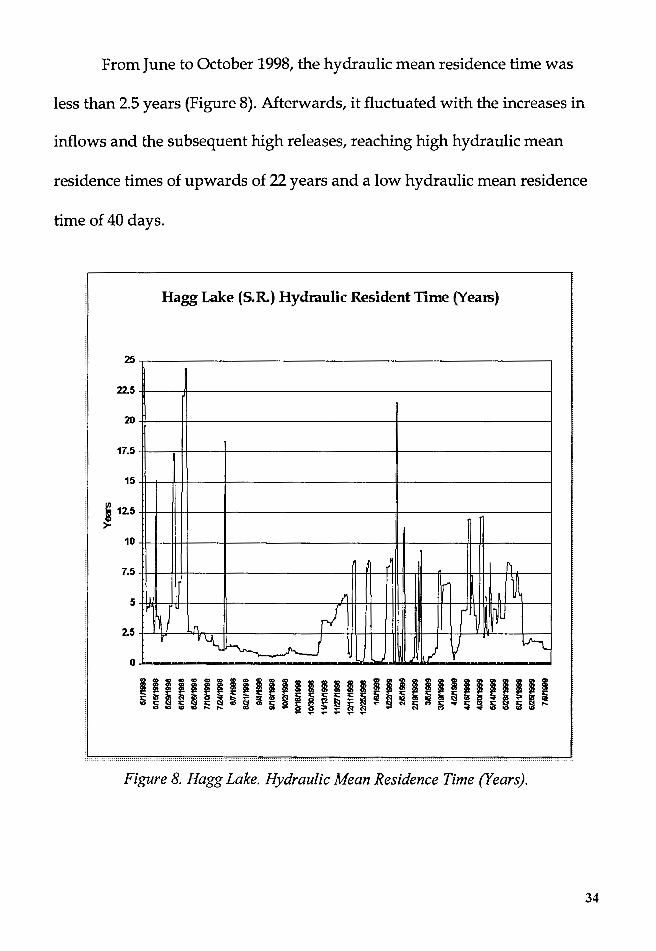
From June to October 1998, the hydraulic mean residence time was
less than 2.5 years (Figure 8). Afterwards, it fluctuated with the increases in
inflows and the subsequent high releases, reaching high hydraulic mean
residence times of upwards of 22 years and a low hydraulic mean residence
time of 40 days.
25
22.5
20
17.5
15
i 12.5 >-
10
7.5
5
2.5
0
Hagg Lake (S.R.) Hydraulic Resident 'lime (Years)
) ri _,.
I~ I I
~ I ~ r ~l 11
r '~~ 1.l ~ """-
m I I I I I I m m ! I I ! I I I I m I ; ! m I ; ! I I I I m ~ ~ i ~ ~ a ~ ~ ~ ~ ~ ~ ~ ~ ~ ~ 5 ti ~ 5 ~ 5 ~ ~ a ~ ~ ~ ~ ~ m 5 m ~ ~ ~ ~ ~ ~ i ~ a ~ ~ ~ ~ ~ - ~ ~ ~ M ~ ~ ~ 5 ~ ~ ~ ~ -- --- -
Figure 8. Hagg Lake. Hydraulic Mean Residence Time (Years).
34
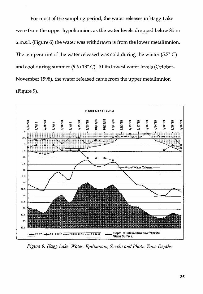
For most of the sampling period, the water releases in Hagg Lake
were from the upper hypolimnion; as the water levels dropped below 85 m
a.m.s.1. (Figure 6) the water was withdrawn is from the lower metalimnion.
The temperature of the water released was cold during the winter (5.7° C)
and cool during summer (9 to 13° C). At its lowest water levels (October-
November 1998), the water released came from the upper metalimnion
(Figure 9).
Hagg Lake (S.R.)
.. .. .. m m m m m ~ ~ ~ m ~ ~ ~ ~ ~ ~ ~
2?. : !!?. : !!?. : !!?. !?. ;:;;- ;;- ~ !?. !!!. !!?. !!?. !?. !!. !!. !!?. M ~ Q ~ ~ ~ ~ ~ ~ N ~ ~ ~ ~ ~ ~ N ~ ~
~ ~ ~ ~ ~ ~ ~ ~ g ~ ~ N ~ ~ ~ ~ ~ ~ ~ ~ ~ ~ ~ ~ ~ m m - - - ~ - N M T ~ ~ ~
0
~: ::\:}TT t~ :::t ::~ i :;! :::T::bn: :)E : . :!: ' :Ln ' .!; :::'uWdLL t ::: :~ 2.5
7.5 'f1\JJl :; • :: :i ;WilHl?'t • HHJ; H•HH#(H ~ I I ~ ~ 10 t-~~~~~~~~~~~~~~~-<111-~~~~"o::::::--~-r~~~~~~~~~~~-t-~~~~---i
12.5 +-~~~~~~~~~~~~~~/C-~~~-:l\.~~~....,,,."'-~->11--~~~~~~~~~~~-+-~~~~~--l
15
17.5 t-~~~~~~..,,....~~~~~t--~~~~~~~~~~~~~t-~~....-~~~~~~~~-t-~~~~~--t
20 +-~~~~~+-~~~~~~~~~~
22.5 I =-......-!
25
27.5
30
32.5
35
37.5
1--Depth ..._Epi·depth -+-PhoticZone _,,,_secchi I __ Depth of lntakeStructurefromthe Water Surface.
Figure 9. Hagg Lake. Water, Epilimnion, Secchi and Photic Zone Depths.
35

2. Temperature
Hagg Lake had a strong temperature stratification that began in May
and lasted through the middle of November. From the end of November to
early May Hagg Lake was under constant mixing due to strong winds
associated with synoptic cycles or cold fronts, and due to increased inflows
of Scoggins, Sain and Tanner Creeks.
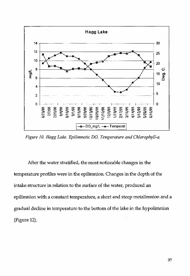
The epilimnetic temperature had a high of 25.2° C in August 1998 and
a low of 5.8° C in February 1999. The temperature graph had a sinusoidal
shape with a maxima and minima occurring at around two months after the
longest and shortest days of the year (Figure 10).
The seasonal temperature isotherms (Time-depth) graph shows the
extent of the stratification and its depths. The influence of the changing
depth levels is reflected in the relatively cool hypolimnion, which changed
from 7° C in June 1998 to 8.6° C in October 1998. The depth of the epilimnetic
layer increased as the water level dropped, and as more water from the
metalimnion was released through the intake structure (Figure 11).
36
Hagg Lake
::1¥0 ~' -~~~-F 20
~ : I --'Ir""~ :s
c: L t 15 l 10
41 • L
ls ~ 2
0 0 00 00 00 00 00 00 00 00 00 00 00 00 en en en en en en en en en en en en en en en en en en en en en en en en en en ..._ ..._ ..._ ..._ ..._ ..._ ..._ ..._ ..._ ..._ ..._ ..._ ..._ ..._ ..._ ..._ ..._ ..._ ..._ ("') !'- 0 .... 00 ..-- LO en ("') 00 0 ("') en !'- tD .... N tD tD N
..._ N
..._ ..-- ..._ ..-- N ..-- N i::::. ..._ ..-- ..-- ..-- i::::. ..-- N ..--..._ !'- ..._ 00 ..._ en ..._ ..._ ..._ ..._ N -... ..._ ..._ ..._ ..._ ..._
tD !'- 00 en en 0 0 ..-- ..-- ..-- N ("') .... LO LO tD ..-- ..-- ..--
1--o- DO_mg/L - Temperat I Figure 10. Hagg Lake. Epilimnetic DO, Temperature and Chlorophyll-a.
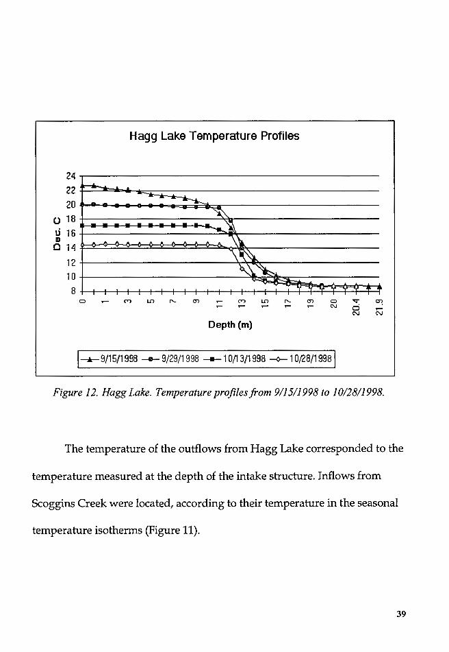
After the water stratified, the most noticeable changes in the
temperature profiles were in the epilimnion. Changes in the depth of the
intake structure in relation to the surface of the water, produced an
epilimnion with a constant temperature, a short and steep metalimnion and a
gradual decline in temperature to the bottom of the lake in the hypolimnion
(Figure 12).
37

w
00
5
10
.s 1
5
.c - a. v 0
20
25
30
6/2
3/9
8
8/4
/9 8
Ha
gg
La
ke (
S.R
.) T
em
pera
ture D
ata
(°C
)
9/1
6/9
8
... ... "' !"
1 0
/2 9
/9 8
1
2 /1
1 /
9 8
.-.~-·
l·
( .•
•·
t .
1/2
3/9
9
3/7
/9 9
4
/19
/99
Sa
m p
iing
Da
te
• P
lace
men
t of S
cog
gin
s C
reek
lnn
ow
s B
y W
ater
Tem
pera
ture
. D
epth
of
Inta
ke S
truc
ture
fro
m th
e ---
Wat
er S
urfa
ce.
Fig
ure
11.
Hag
g L
ake.
Tim
e-de
pth
grap
h o/
Tem
pera
ture
(°C
).
~-----------------·----------
6/1
/99
24 22 20
(.) 18 u 16 II)
0 14
12 10 8
C)
Hagg Lake Temperature Profiles
("") LO I"- 01 .-- ("") LO .....
Depth (m)
I".-
01 ..... C) ... (.'J •
Cl N
1~9/15/1998 __._ 9/29/1998 - 10/13/1998 ---¢--10/28/19981
en .-N
Figure 12. Hagg Lake. Temperature profiles.from 911511998to1012811998.
The temperature of the outflows from Hagg Lake corresponded to the
temperature measured at the depth of the intake structure. Inflows from
Scoggins Creek were located, according to their temperature in the seasonal
temperature isotherms (Figure 11 ).
39
---,
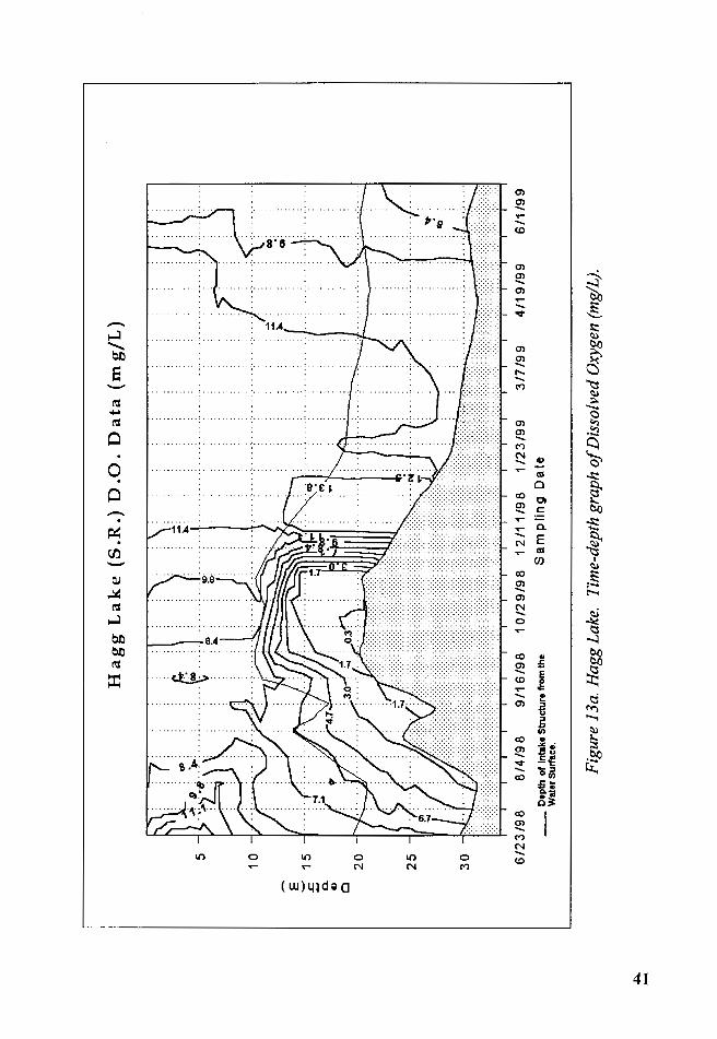
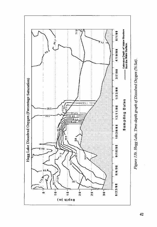
3. Dissolved Oxygen
The epilimnetic layer was oxygenated throughout the year, with a low
concentration of 7.5 mg/Lin August and a high concentration of 12.2 mg/L
in April 1999. The highest levels of dissolved oxygen occurred from
November 1998 to May 1999. The peak levels of dissolved oxygen coincided
with the peak values in chlorophyll-a indicating the strong influence of the
photosynthetic activity of the phytoplankton.
The effects that the changes in depth of intake structure depth relative
to the water surface had on dissolved oxygen was as follows: with water
withdrawn from higher and higher layers of water, a pocket of anoxic water
appeared near the bottom of the lake. From 8/18/1998to10/28/1998, the
water levels were at their lowest and a layer of anoxic water 4.5 m thick was
measured on October 13, 1998.
These low water levels isolated the hypolimnion from withdrawals of
the intake structure contributing to the formation of a clinograde curve of
D.O. with low values measured at the depth of the intake structure that
decrease further as they are measured near the bottom of the reservoir, until
reaching the anoxic layer (Figure 13a and 13b). In figure 11, the placement
according to their temperature of the waters entering the reservoir through
Scoggins Creek is portrayed. Their dissolved oxygen contribution appeared
limited to the depths at which they were placed.
40
,,., ,_.
Hag
g L
ak
e (
S.R
.) D
.O.
Data
(m
g/L
)
~ sr:E~
.. :r=
J\ . .
. .
. .
.
: fl
:
. .
. .
1 0
~
E
:;;
15
- 0. Q
)
0 2
0
25
30
6/2
3 /9
8
8/4
/9 8
9
/16
/98
1
0/2
9/9
8
12
/11
/98
1
/23
/99
__
Dep
th o
f In
take
Str
uctu
re f
rom
the
Wat
er S
urfa
ce.
Sa
mp
lin
g D
ate
3/7
/9 9
4
/19
/99
Fig
ure
J 3a.
Hag
g La
ke.
Tim
e-de
pth
grap
h o
f Dis
solv
ed O
xyge
n (m
g/L)
.
6/1
/99
.io.
N
5
10
E
.s::: ~
15
Q
) c
30
6/2
3/9
8
8/4
/98
Hag
g L
ake
Dis
solv
ed O
xy
gen
(P
erce
ntag
e S
atur
atio
n)
9/1
6/9
8
10
/29
/98
1
2/1
1/9
8
112
3/9
9
Sa
m p
iin
g D
ate
s
3/7
/99
4
/19
/99
6
/1 /
99
Est
imat
ed D
epth
of
Inta
ke S
truc
ture
---
from
the
Wat
er S
urfa
ce.
Fig
ure
13b.
Hag
g La
ke.
Tim
e-de
pth
grap
h o
f Dis
solv
ed O
xyge
n (%
Sat)
.

4. Secchi depth and Irradiance
In Hagg Lake the Secchi depth was greater from June to the end of
October 1998. The highest Secchi depth was measured on August 18, (4.3 m)
and September 29, 1998. The average Secchi depth form June to October 28,
1998 was 2. 9 m. The Secchi depth decreased with the beginning of the winter
storms and had a low of 0.4 min March 1999(Figure14).
Hagg Lake
00 00 00 00 co 00 01 01 m en en en (5) (5) en (5) en en en (5) (5) (5) en en m en ..-- ..-- m en en en ..-- ..-- c ..-- - - c z:::::. ..-- z:::::. "-- "-- "-- ("") C) "--("") C) co LO ..-- ..-- m = C'J = C'J C'J .- ~ - - .- ~ .-- ~ ....._ ....._ ...._ C) ,... ...._ ....._ = I"'- co en .-- .-- .- ("") LO =
0 I I I I I I I I I I I I I I I I I I 1- I 0 1 10 2 3 20
Cl) 4 30 ~ .....
E 5 z 6 40 7 8
50
9 60
1---tr-Secchi -----EuphoticZone --.-NTU_Turb I
Figure 14. Hagg Lake. Secchi and Photic depth.
43
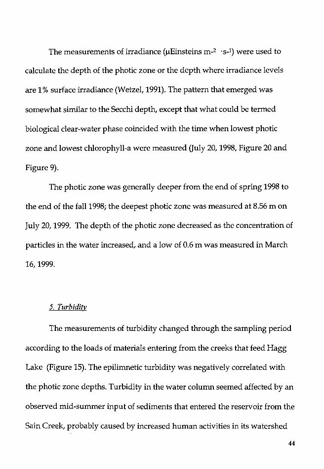
The measurements of irradiance (µEinsteins m-2 ·s-1) were used to
calculate the depth of the photic zone or the depth where irradiance levels
are 1 % surface irradiance (Wetzel, 1991). The pattern that emerged was
somewhat similar to the Secchi depth, except that what could be termed
biological clear-water phase coincided with the time when lowest photic
zone and lowest chlorophyll-a were measured Guly 20, 1998, Figure 20 and
Figure 9).
The photic zone was generally deeper from the end of spring 1998 to
the end of the fall 1998; the deepest photic zone was measured at 8.56 m on
July 20, 1999. The depth of the photic zone decreased as the concentration of
particles in the water increased, and a low of 0.6 m was measured in March
16, 1999.
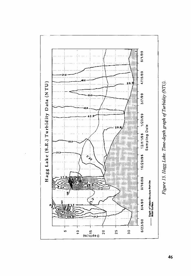
5. Turbidity
The measurements of turbidity changed through the sampling period
according to the loads of materials entering from the creeks that feed Hagg
Lake (Figure 15). The epilimnetic turbidity was negatively correlated with
the photic zone depths. Turbidity in the water column seemed affected by an
observed mid-summer input of sediments that entered the reservoir from the
Sain Creek, probably caused by increased human activities in its watershed
44

(logging or road construction). These mid-summer events occurred July 20
and September 19, 1998, and in these occasions the maximum turbidity
readings in the water column were 141and195 NTU respectively. Some rain
events, road construction or clear-cutting occurred around these dates. From
these events it was evident that small human impacts on the watershed
during the dry season had a greater impact on turbidity than during the
rainy season when sediments and other materials entering the reservoir are
diluted in large volumes of water.
45
.,. 0-.
5
10
~
E
:5 1
5 0
..
G>
Cl 2
0
25
30
Hag
g L
ak
e (
S.R
.) T
urb
idit
y D
ata
(N
TU
)
6/2
3/9
8
8/4
/9 8
9
/16
/98
1
0/2
9/9
8
1 2
/11
/98
1
/23
/99
3
/7 /9
9
4/1
9/9
9
__
_ D
epth
of
Inta
ke S
tru
ctu
re f
rom
the
Wat
er S
urfa
ce.
Sa
mp
lin
g D
ate
Fig
ure
15.
Hag
g La
ke.
Tim
e-de
pth
grap
h o
f Tur
bidi
ty (
NTU
) .
6/1
/9
9
b) Chemical factors
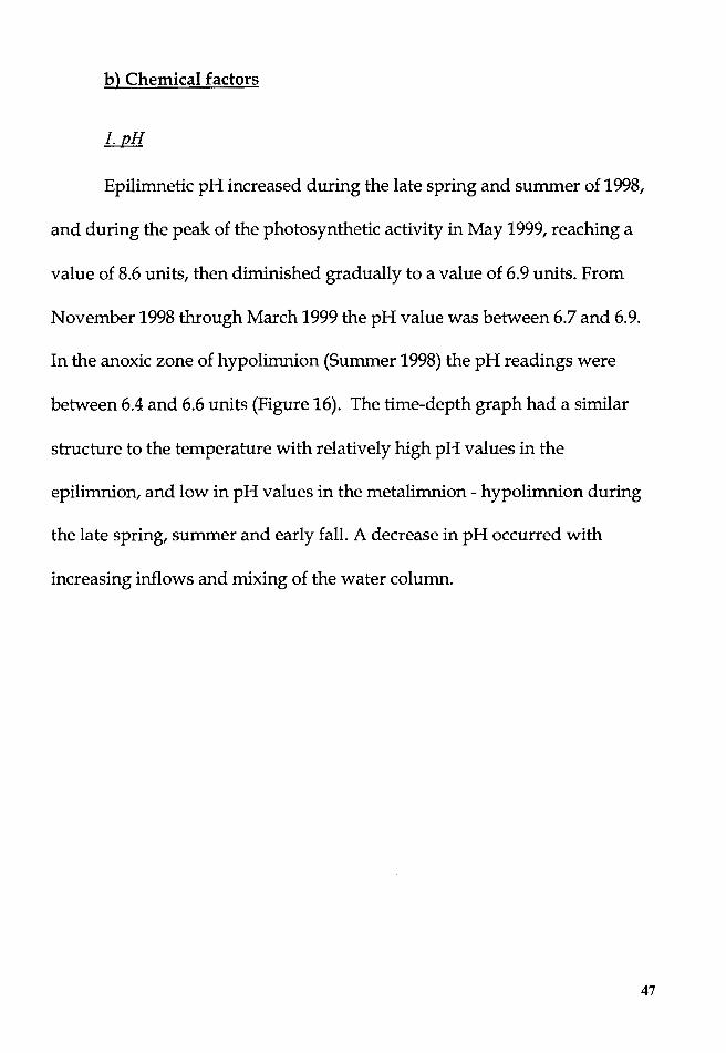
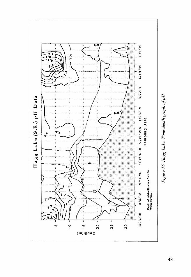
1. pH
Epilimnetic pH increased during the late spring and summer of 1998,
and during the peak of the photosynthetic activity in May 1999, reaching a
value of 8.6 units, then diminished gradually to a value of 6.9 units. From
November 1998 through March 1999 the pH value was between 6.7 and 6.9.
In the anoxic zone of hypolimnion (Summer 1998) the pH readings were
between 6.4 and 6.6 units (Figure 16). The time-depth graph had a similar
structure to the temperature with relatively high pH values in the
epilimnion, and low in pH values in the metalimnion- hypolimnion during
the late spring, summer and early fall. A decrease in pH occurred with
increasing inflows and mixing of the water column.
47
~
QO
5
10
E ~
15
a.
Q
)
0 2
0
25
30
Ha
gg
La
ke (
S.R
.) p
H D
ata
Q •l
) ()
--~°!···
····
.. ! ..
. l
.. l
6/2
3/9
8
8/4
/9 8
9
/16
/98
1
0/2
9/9
8
12
/11
/98
1
/23
/99
3
/7 /9
9
Dep
th o
f In
take
Str
uctu
re f
rom
the
---
Wat
er S
urfa
ce.
Sa
m p
iin
g D
ate
Fig
ure
16.
Hag
g La
ke.
Tim
e-de
pth
grap
h o
f pH
/\
. io
. : .
a>
4/1
9/9
9
6 /1
/99
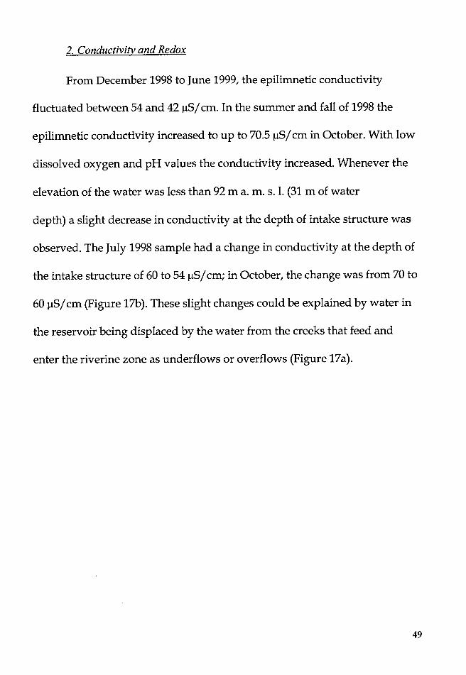
2. Conductivity and Redox
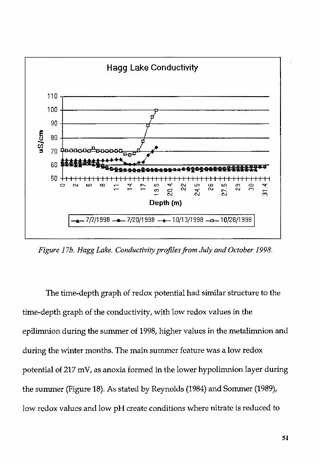
From December 1998 to June 1999, the epilimnetic conductivity
fluctuated between 54 and 42 µS/ cm. In the summer and fall of 1998 the
epilimnetic conductivity increased to up to 70.5 µS/ cm in October. With low
dissolved oxygen and pH values the conductivity increased. Whenever the
elevation of the water was less than 92 ma. m. s. l. (31 m of water
depth) a slight decrease in conductivity at the depth of intake structure was
observed. The July 1998 sample had a change in conductivity at the depth of
the intake structure of 60 to 54 µS/ cm; in October, the change was from 70 to
60 µS/ cm (Figure 17b). These slight changes could be explained by water in
the reservoir being displaced by the water from the creeks that feed and
enter the riverine zone as underflows or overflows (Figure 17a).
49

u-. =
5 ..
. .,; :· ~+- •
10
E
Hag
g L
ak
e (
S.R
.) C
on
du
cti
vit
y D
ata
(u
S/c
m)
c:n:
.....
.• ..... •
,... ..
~. '°
.,,. -:
~:
~ ...
····
····
··.·
···.
··
--~·
'•'
:;;
15
i:
a ......
- Cl. Q)
0 2
0
-_;_;~
25
30
6/2
3/9
8
8/4
/98
9
/16
/98
1
0/2
9/9
81
2/1
1/9
8
1/2
3/9
9
3/7
/99
4
/19
/99
6
/1/9
9
De
pth
of
Inta
ke S
tru
ctu
re f
rom
the
---
Wat
er S
urfa
ce.
Sa
m p
iin
g D
ate
•
Pla
cem
en
t of S
cog
gin
s C
reek
lnft
ow
s B
y W
ater
Te
mp
era
ture
.
Fig
ure
17
a. H
agg
Lak
e. T
ime-
dept
h gr
aph
of C
ondu
ctiv
ity
(µSi
em).
110
100
90
e 80 u -Cl)
::3 70
60
50 0 N LO co
Hagg Lake Conductivity
V ~ ~ V N ~ ~ LO ~ 0 V ~ ~ Q N V N ~ N M ~
~ N N N M
Depth (m)
,_.__ 11111998-e-112011998 -+-10113/1998 --a--1012011990 I
Figure I 7b. Hagg Lake. Conductivity profiles from July and October 1998.
The time-depth graph of redox potential had similar structure to the
time-depth graph of the conductivity, with low redox values in the
epilimnion during the summer of 1998, higher values in the metalimnion and
during the winter months. The main summer feature was a low redox
potential of 217 mV, as anoxia formed in the lower hypolimnion layer during
the summer (Figure 18). As stated by Reynolds (1984) and Sommer (1989),
low redox values and low pH create conditions where nitrate is reduced to
51

ammonia, and other nutrients are released from the sediments into the
waters. These nutrients can reach the epilimnion and cause blooms of algae
that might interfere with the water treatment and human consumption of
these waters. In Hagg Lake an increase in hypolimnetic ammonium was
observed during the period of anoxia and low redox potential.
52

Ul ~
5
1 0
E
:;;
1 5
Cl.
<I)
Cl
20
25
30
Hag
g L
ak
e (
S.R
.) R
ed
ox
Data
(m
V)
6/2
3/9
8
8/4
/9 8
9
/16
/98
1
0/2
9/9
8
12
/11
/98
1
/23
/99
Sa
mp
lin
g D
ate
3/7
/9 9
4
/19
/99
--
De
pth
of
Inta
ke S
truc
ture
fro
m th
e W
ate
r Sur
face
.
Fig
ure
18.
Hag
g L
ake.
Tim
e-de
pth
grap
h o
f Red
ox P
oten
tial
(m V
).
6/1
/99
------------~---------------·--------------------·------------------------------------------'

3. Alkalinity and Dissolved Inorganic Carbon (DIC)
Alkalinity (Acid Neutralizing Capacity) was measured in
µEquivalent/L units. Average epilimnetic alkalinity from June to October
1998 was calculated at 582 µEq/L. From October 1998 to June 1999 the
average was 533 µEq/L. The highest alkalinity was measured in August
1998. This increase was concurrent with an increase in conductivity (Figure
19a). From June to July 1998 and April to June 1999, measured epilimnetic
and hypolimnetic alkalinity were similar. The summer 1998 and winter 1999
measured epilimnetic and hypolimnetic alkalinity were different, and these
differences appeared related to changes in water levels and inflows.
The summer 1998 distribution of DIC in the water column seemed
affected by biological reactions (Wetzel 1983). The dissolved inorganic
carbon (DIC) was derived from pH and alkalinity measurements (Wetzel
and Likens, 1991). The trends of DIC followed the trends of alkalinity, and
had a calculated high concentration of 0.22 mg C/L in August 1998. Other
high values were measured in October 1998 and February 1999. DIC was
higher in the metalimnion and hypolimnion, except during late Fall 1998 and
winter 1999 when it was either equal or lower than the calculated epilimnetic
DIC (Figure 19b).
54
mg
C/L
u
Eq
/L
~
!==>
0 0
0 0
0 c..>
~
(11
(1
) "'-
! CX
> CD
0
0 0
0 0
0 0
s:: 0
.....
N
<..>
~
<.n
en 0
0 0
0 0
0 0
""'I
6/23
/98
6/23
/98
(I:> ........
. \Q
7/
7/98
~
7/7/
98
SJ"' ~
7/20
/98
~·
7/20
/98
s:: ""'I
~
(I:>
t 8/
4/98
.....
.... 8/
4/98
t--
< \Q
s:::
i 8/
18/9
8 ~
t 8/
18/9
8 ~
m
'C
~ :c
~
~r
9/1/
98
:c
~
m
9/1/
98
1:11
-· ::
I 1:1
1 'C
cc
~
9/15
/98
9/15
/98
~
O'
cc
t--<
~r
cc
0 ::
I cc
s:::
i ~
::I
r (I:
>
+
9/29
/98
r ~
a· 9/
29/9
8 $:)
,.. 1:1
1 ::
I )>
~
10/1
3/98
~
::i....
t 10
/13/
98
s:: C1
)
~ ~
0 CD
c
1:11
~
!if
10/2
8/98
.....
s::
10/2
8/98
-·
::s
s:::i
~~j'
(')
~
CD
;:::;:
~
11/1
0/98
-·
!if
11/1
0/98
-.
::I
~
'<
(',)
5·
3·
g ::
I 12
/3/9
8 ~
::I
12/3
/98
t ~
a· ""'
I ::
I CJ
" 1/
19/9
9 1 /
19/9
9 0
~
+
~
I ':-
--
~
'<
2/17
/99
2/17
/99
'C
0 I
~
3· 3/
16/9
9 '<
3/
16/9
9 Q
'C
::
I 0
~
5·
4/14
/99
3· 4/
14/9
9 ::
I ::
I
5/12
/99
a· 5/
12/9
9 ::
I
5/26
/99
5/26
/99
Ul
I 6/
16/9
9 6/
16/9
9 U
l
---------------------------------·-··-·-··----.--
.. -------·
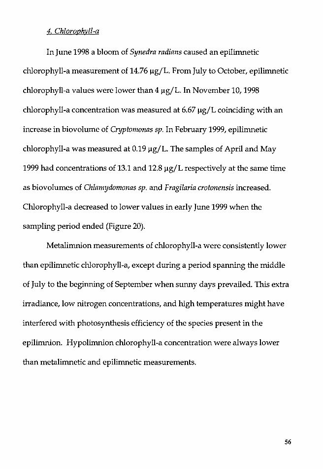
4. Chlorophyll-a
In June 1998 a bloom of Synedra radians caused an epilimnetic
chlorophyll-a measurement of 14.76 µg/L. From July to October, epilimnetic
chlorophyll-a values were lower than 4 µg/L. In November 10, 1998
chlorophyll-a concentration was measured at 6.67 µg/L coinciding with an
increase in biovolume of Cryptomonas sp. In February 1999, epilimnetic
chlorophyll-a was measured at 0.19 µg/L. The samples of April and May
1999 had concentrations of 13.1and12.8 µg/L respectively at the same time
as biovolumes of Chlamydomonas sp. and Fragilaria crotonensis increased.
Chlorophyll-a decreased to lower values in early June 1999 when the
sampling period ended (Figure 20).
Metalimnion measurements of chlorophyll-a were consistently lower
than epilimnetic chlorophyll-a, except during a period spanning the middle
of July to the beginning of September when sunny days prevailed. This extra
irradiance, low nitrogen concentrations, and high temperatures might have
interfered with photosynthesis efficiency of the species present in the
epilimnion. Hypolimnion chlorophyll-a concentration were always lower
than metalimnetic and epilimnetic measurements.
56
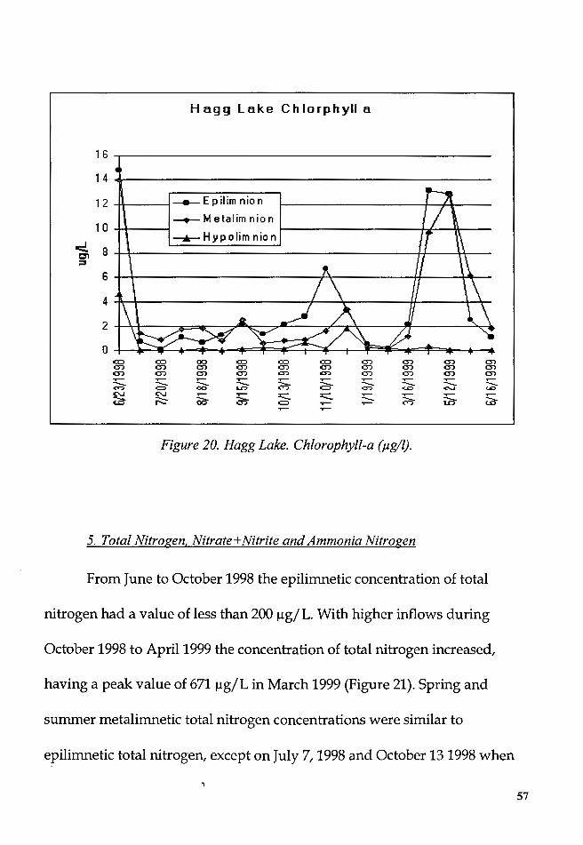
Hagg Lake Chlorphyll a
16
14
12 1• , ____ E p ii im n ion
10 --1'- M etalim nion
I ) I
-=:!. 8 i:;,'I
_...,_ Hypolim nion
;::,
6
4
2
0 co co co co co co O') O') O') = O') O') = O') O') O') O') O') O') = O') O') = O') """ """ O') O') O') = ..-----~ ..-- .-- ..--
~ ~ ..-- ..-- ..-- .----- ......_ --- --- --- --- ......_
c:> 00 ..,,,, oO? -<.:::> ........ u:> C'\J (:a-
C'\J
~ ..-- :r::::. :r::::. ..-- ..-- i:a- £-~ ;:n- --- ~ c:::> ..-- ..--..--
Figure 20. Hagg Lake. Chlorophyll-a (µg/l).
5. Total Nitrogen, Nitrate+Nitrite and Ammonia Nitrogen
From June to October 1998 the epilimnetic concentration of total
nitrogen had a value of less than 200 µg/L. With higher inflows during
October 1998 to April 1999 the concentration of total nitrogen increased,
having a peak value of 671 µg/L in March 1999 (Figure 21). Spring and
summer metalimnetic total nitrogen concentrations were similar to
epilimnetic total nitrogen, except on July 7, 1998 and October 131998 when
57
the concentrations were much higher. On these occasions rain events had
occurred in the previous week, and underflow waters could have carried a
delayed nutrient pulse. From October 1998 to April 1999 epilimnetic total
nitrogen increased with a high measurement of 671 µg/L.
Summer hypolimnetic total nitrogen was always greater than the
epilimnetic measurements. From October 1998 to April 1999 hypolimnetic
concentrations of total nitrogen were similar to epilimnetic and metalimnetic
concentrations, but from May to June 1999, the total nitrogen concentration
in the hypolimnion remained high while epilimnetic and metalimnetic total
nitrogen decreased. The explanation offered at this time by the author is that
wind induced mixing and high water inflows homogenized the distribution
of total nitrogen in the water column.
58
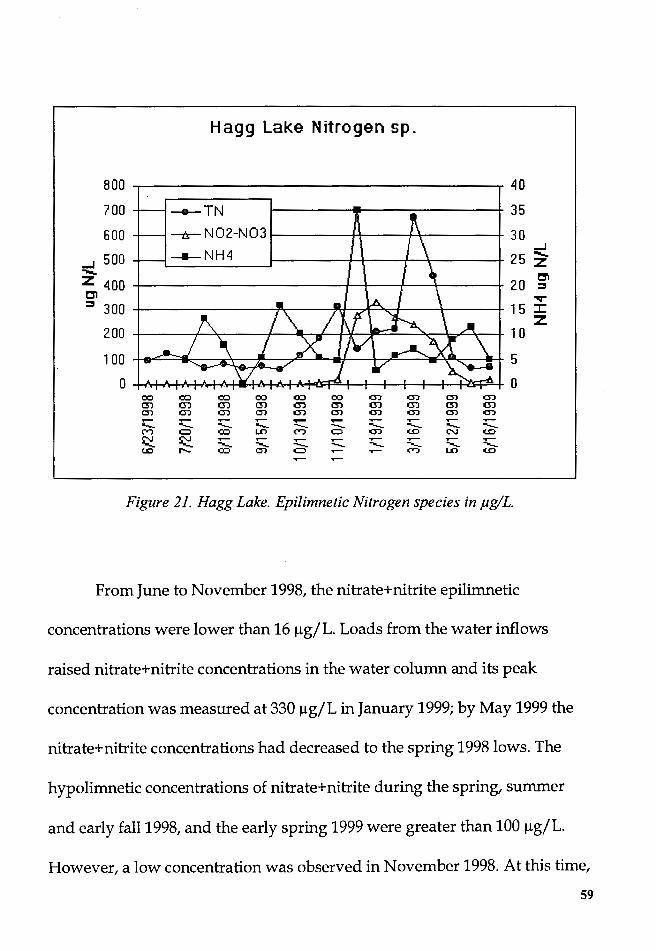
Hagg Lake Nitrogen sp.
800 40
700 _._TN 35
600 --n-N02-N03 30
---NH4 ....J
....J 500 25 z
....... "' z 400 20 ::I
Cl """ ::I 300 1 5 :I: z 200 10
100 5
0 0 00 co co 00 co 00 C') C') = C')
C3"J OJ OJ C3"J ~ = OJ OJ C3"J OJ = C') C') = C') = C') C') = C')
.- ..-- ..-- .- ..... .... ..-- ..-- .- ..--...._ ..._ ..._ ...._ - -- ..._ ..._ ...._ ..._ M C) co U"l ("") = C') (.0 C'J (.0
C'J oC\J ~ ' ..-- .- ~ ~
.- ..--...._ ....._ - -- ...._ ....._ U) ...,_ co = C) .- ..-- ("") U"l (.0
Figure 21. Hagg Lake. Epilimnetic Nitrogen species in µg/L.
From June to November 1998, the nitrate+nitrite epilimnetic
concentrations were lower than 16 µg/L. Loads from the water inflows
raised nitrate+nitrite concentrations in the water column and its peak
concentration was measured at 330 µg/L in January 1999; by May 1999 the
nitrate+nitrite concentrations had decreased to the spring 1998 lows. The
hypolimnetic concentrations of nitrate+nitrite during the spring, summer
and early fall 1998, and the early spring 1999 were greater than 100 µg/L.
However, a low concentration was observed in November 1998. At this time,
59

low redox potential and low D.0. was observed in the hypolirnnion. High
water inflows were beginning to occur while water releases decreased; at the
same time a peak in biovolumes of Cryptomonas sp. occurred in the
epilirnnion.
Ammonium nitrogen concentrations in the water column were lower
than 50 µg/L throughout the sampling period, except for a noticeable
increase in the hypolimnetic ammonium during the anoxic period as
nitrate+nitrate was reduced. At this time ammonium nitrogen concentration
reached a maxima of 195 µg/L (11/13/1998). With increases in inflows, the
concentration of ammonium nitrogen decreased again to low levels
6. Total Phosphorous and Soluble Reactive Phosphorous
Total phosphorous concentrations seemed to be controlled by the
water levels (inflows) and water pH. Epilimnetic, metalimnetic and
hypolimnetic values had similar seasonal patterns. Epilimnetic total
phosphorous had a high concentration of 29 µg/L (June 23, 1998), it
decreased to 7 µg/L and increased again as low dissolved oxygen conditions
occurred in the hypolirnnion (Figure 22).
60
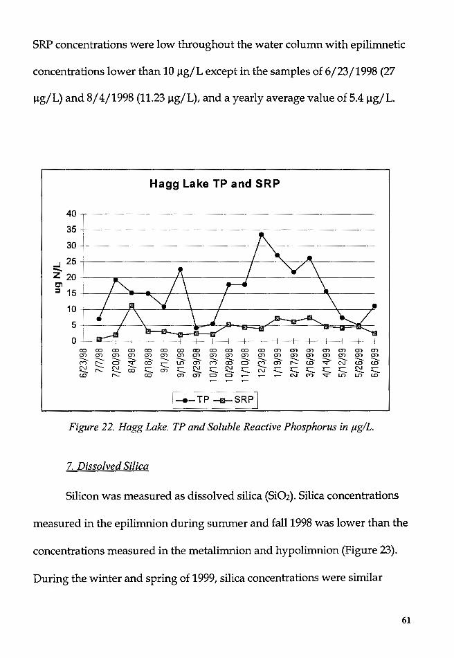
SRP concentrations were low throughout the water column with epilimnetic
concentrations lower than 10 µg/L except in the samples of 6/23/1998 (27
µg/L) and 8/ 4/1998 (11.23 µg/L), and a yearly average value of 5.4 µg/L.
Hagg Lake TP and SRP
40~~~~~~~~~~~~~~~~~~~~~~
35-+-~~~~~~~~~~~~~~~~~~~~-
30-+-~~~~~~~~~~~~-+-~~~~~~~~
~ 25+-~~~~~~~~~~~~__,~~--~---~~~~~ -z 20 -t----...------r-+---------.1-------'1------C'I ::I 15 +---1----....... -.--1------i.----+--------~----
10 •
5 I I \::: ......_ _. ,.,s -m=:iii'....- ... "m- m ::a.: 0
co ro co co co co co ro ro ro ro co en en en en en en en en en en en en en en en en en en en en en en en en en en - - - - - - - - - - - - - - - - - - -M I'- C) v co .-- Ln en M co C) ("") en I'- U) v N (.0 U)
N - N - .-- - ,....- N .-- N .-- - ,....- .-- .-- ,....- .-- N .--- I'- - co - en - - - - - N - - - - - - -U) I'- co en en C) C) .-- ,....- .-- N ("") v LO Ln U)
I---TP -m-SRP I Figure 22. Hagg Lake. TP and Soluble Reactive Phosphorus in µg!L.
7. Dissolved Silica
Silicon was measured as dissolved silica (Si02). Silica concentrations
measured in the epilimnion during summer and fall 1998 was lower than the
concentrations measured in the metalimnion and hypolimnion (Figure 23).
During the winter and spring of 1999, silica concentrations were similar
61
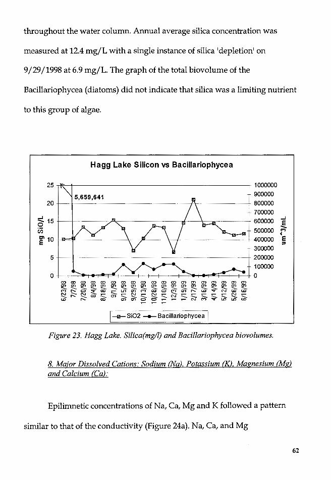
throughout the water column. Annual average silica concentration was
measured at 12.4 mg/L with a single instance of silica 'depletion' on
9/29/1998 at 6.9 mg/L. The graph of the total biovolume of the
Bacillariophycea (diatoms) did not indicate that silica was a limiting nutrient
to this group of algae.
Hagg Lake Silicon vs Bacillariophycea
25~-+-~~~~~~~~~~~~~~---i-
5,659,641 20+---+~~~~~~~~~~~~----f4,~~~~~--+
=:!. 15 +--, -0 (:jj
~ 10
5-+--+~~~~~~~~~~~~~~~~~~~--+-
0 I I -J'-e • • ff I • I =-i--. • ...,...... I ... I CD a:> CD a:> CD en en en en en ---------(T') I'- 0 V CD
~f::-~00-c (D "" (X)
CD a:> a:> CD en en en en -- -- -- -r- LO C") ('V")
en :c:.. ~ :c:.. en en o
a:> CD a:> en en en en en en en -- -- -- -- -CD 0 ("") en I'-
~ :c:.. N- :c:.. c 0 r- .,.- r- N
en en en en en en en en en en -- -- -- -- -(D v C'J (D (D r- r- r- N .,.--- -- -- -- -("") V LO LO tD
1--e-Si02 --+-- Bacillariophycea I
1000000 900000 800000 700000 600000 500000 400000 300000 200000 100000 0
Figure 23. Hagg Lake. Silica(mg/l) and Bacillariophycea biovolumes.
..J E -t"')
(
E :I
8. Major Dissolved Cations: Sodium (Na), Potassium (K), Magnesium (Mg) and Calcium (Ca):
Epilimnetic concentrations of Na, Ca, Mg and K followed a pattern
similar to that of the conductivity (Figure 24a). Na, Ca, and Mg
62
concentrations were greater than 1 mg/L. The concentrations of K never
reached beyond 0.4 mg/L.
Ca had greater concentrations from June to December 1998 with high
concentrations in July and November, followed by a decrease (1.7 mg/L in
Feb. 1999) and a slow increases afterwards.
Na concentrations were greater from June and December 1998 with
higher concentrations in September 1998 (6.5 mg/Lin 9/29/1998), followed
by a decrease in February 1999 (2.78 mg/L} and a slow increase in
concentration.
K had an initial concentration of 0.34 mg/Land a low concentration of
0.14 mg/Lin September. Overall, the concentrations of K from June to
December 1998 were greater than the winter and spring 1999 concentrations.
Concentrations of Mg were greater from June and December 1998
with a high concentration in November 1998 (2.45 mg/L), followed by a
decrease in February 1999 (1.2 mg/L) and slow increase in concentration.
Late spring, summer and fall 1998 concentrations were higher that
winter concentrations. This could have been the result of outflow levels that
were kept constant while inflows diminished rapidly. Another possibility is
that as the sediments settled, the temperatures rose, and changes in pH and
redox potential occurred in the reservoir, more cations were released from
63
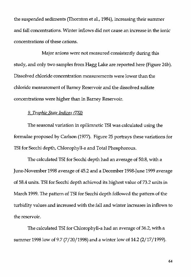
the suspended sediments (Thornton et al., 1984), increasing their summer
and fall concentrations. Winter inflows did not cause an increase in the ionic
concentrations of these cations.
Major anions were not measured consistently during this
study, and only two samples from Hagg Lake are reported here (Figure 24b).
Dissolved chloride concentration measurements were lower than the
chloride measurement of Barney Reservoir and the dissolved sulfate
concentrations were higher than in Barney Reservoir.
9. Trophic State Indices O'S!)
The seasonal variation in epilimnetic TSI was calculated using the
formulae proposed by Carlson (1977). Figure 25 portrays these variations for
TSI for Secchi depth, Chlorophyll-a and Total Phosphorous.
The calculated TSI for Secchi depth had an average of 50.8, with a
June-November 1998 average of 45.2 and a December 1998-June 1999 average
of 58.4 units. TSI for Secchi depth achieved its highest value of 73.2 units in
March 1999. The pattern of TSI for Secchi depth followed the pattern of the
turbidity values and increased with the fall and winter increases in inflows to
the reservoir.
The calculated TSI for Chlorophyll-a had an average of 36.2, with a
summer 1998 low of 9.7 (7 /20/1998) and a winter low of 14.2 (2/17 /1999).
64
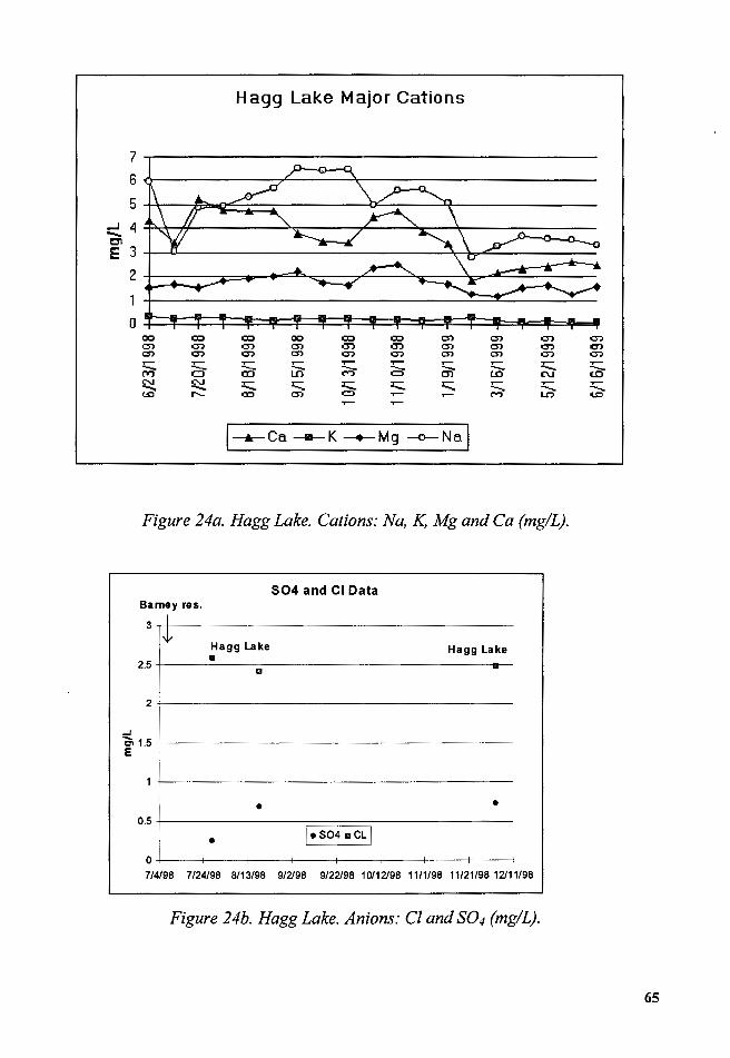
Hagg Lake Major Cations
7
6
5
...J 4 -Cl E 3
2
1
0 CX) co co CX) co co = = ()") ()")
= ()") ()") = (:p (:p = = ()") ()") = ()") ()") = ()") ()") = = ()") ()")
.-- ..-- ..-- .-- .,... .,... .-- .-- ..-- ..--- - - - - - - - - -(Y") a co LO ("") c::> 01 lO C\.J (!) N oC'J ..-- .-- ..-- ..-- .-- c.. :i:::. ..--- ............ ............ - - - - ............ = I"- co = c::> ..-- .-- ("") LO (.0
!__._ca --K -+-Mg -o-Na I
Figure 24a. Hagg Lake. Cations: Na, K, Mg and Ca (mg!L).
504 and Cl Data Barney res.
31± Hagg Lake • Hagg Lake
2.5 El
2
~ -a. 1.5 e
1
• • 0.5
• [ eS04 11CL f
0 7/4/98 7/24/98 8/13/98 9/2/98 9/22/98 10/12/98 11/1/98 11/21/98 12111/98
Figure 24b. Hagg Lake. Anions: Cl and S04 (mg/L).
65
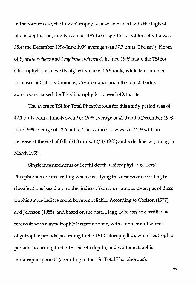
In the former case, the low chlorophyll-a also coincided with the highest
photic depth. The June-November 1998 average TSI for Chlorophyll-a was
35.4; the December 1998-June 1999 average was 37.7 units. The early bloom
of Synedra radians and Fragilaria crotonensis in June 1998 made the TSI for
Chlorophyll-a achieve its highest value of 56.9 units, while late summer
increases of Chlamydomonas, Cryptomonas and other small bodied
autotrophs caused the TSI Chlorophyll-a to reach 49.1 units
The average TSI for Total Phosphorous for this study period was of
42.1 units with a June-November 1998 average of 41.0 and a December 1998-
June 1999 average of 43.6 units. The summer low was of 24.9 with an
increase at the end of fall (54.8 units, 12/3/1998) and a decline beginning in
March 1999.
Single measurements of Secchi depth, Chlorophyll-a or Total
Phosphorous are misleading when classifying this reservoir according to
classifications based on trophic indices. Yearly or summer averages of these
trophic status indices could be more reliable. According to Carlson (1977)
and Johnson (1985), and based on the data, Hagg Lake can be classified as
reservoir with a mesotrophic lacustrine zone, with summer and winter
oligotrophic periods (according to the TSI-Chlorophyll-a), winter eutrophic
periods (according to the TSI- Secchi depth), and winter eutrophic
mesotrophic periods (according to the TSI-Total Phosphorous).
66
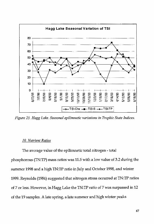
Hagg Lake Seasonal Variation of TSI
ao~~~~~~~~~~~~~~~~~~~~~~~~-
70-+-~~~~~~~~~~~~~~~~------T~~~~-
60+-~~~~~~~~~~~~~1--~~~~__...,~~~-
508 ... ......___ .J/ ~~At .. / ~
40 I\ \ I ',.P..,,,/ \ '-...,r _;;/ll "\ J "\. 'a \ ..
30 ~ ,,.._, :/' \ ,/; \ I -.... ... / ..
20-+--~+-----1-~~~~~~~~~~~~~~1--~~~~~-
10-+--~-<1>--~~~~~~~~~~~~~~~~~~~~-
0 c:o c:o c:o c:o c:o c:o c:o c:o c:o c:o c:o c:o C") C") C") C") C") C") C") C") C") C") C") C") C") C") C") C") C") C") C") C") C") C") C") C") C") C") ........ ........ ........ ........ ........ ........ ........ ........ ........ ........ ........ ........ ........ ........ ........ ........ ........ ........ ........ ("") I'-- 0 "" c:o ..- LO en ("") c:o 0 ("") C") I'-- U) "" C\J U) U)
C\J ........ C\J ........ ..- ........ ..- C\J ..- C\J ..- ........ ..- ..- ..- ..- i:::. C\J ..-........ I'-- ........ c:o ........ C") ........ ........ ........ ........ ........ C\J ........ ........ ........ ........ ........ ........ U) I'-- c:o C") C") 0 0 ..- ..- ..- C\J ("") "" LO LO U)
j-e-TSl-Cha --TSl-S -+-TSl-TP j
Figure 25. Hagg Lake. Seasonal epilimnetic variations in Trophic State Indices.
10. Nutrient Ratios
The average value of the epilimnetic total nitrogen - total
phosphorous (TN:TP) mass ratios was 11.5 with a low value of 3.2 during the
summer 1998 and a high TN:TP ratio in July and October 1998, and winter
1999. Reynolds (1984) suggested that nitrogen stress occurred at TN:TP ratios
of 7 or less. However, in Hagg Lake the TN:TP ratio of 7 was surpassed in 12
of the 19 samples. A late spring, a late summer and high winter peaks
67
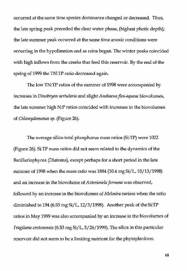
occurred at the same time species dominance changed or decreased. Thus,
the late spring peak preceded the clear water phase, (highest photic depth);
the late summer peak occurred at the same time anoxic conditions were
occurring in the hypolimnion and as rains began. The winter peaks coincided
with high inflows from the creeks that feed this reservoir. By the end of the
spring of 1999 the TN:TP ratio decreased again.
The low TN:TP ratios of the summer of 1998 were accompanied by
increases in Dinobryon sertularia and slight Anabaena fios-aqueae biovolumes,
the late summer high N:P ratios coincided with increases in the biovolumes
of Chlamydomonas sp. (Figure 26).
The average silica-total phosphorus mass ratios (Si:TP) were 1022
(Figure 26). Si:TP mass ratios did not seem related to the dynamics of the
Bacillariophycea (Diatoms), except perhaps for a short period in the late
summer of 1998 when the mass ratio was 1884 (10.4 mg Si/L, 10/13/1998)
and an increase in the biovolume of Asterionela formosa was observed,
followed by an increase in the biovolumes of Melosira varians when the ratio
diminished to 194 (6.53 mg Si/L, 12/3/1998). Another peak of the Si:TP
ratios in May 1999 was also accompanied by an increase in the biovolumes of
Fragi.laria crotonensis (6.53 mg Si/L, 5/26/1999). The silica in this particular
reservoir did not seem to be a limiting nutrient for the phytoplankton.
68
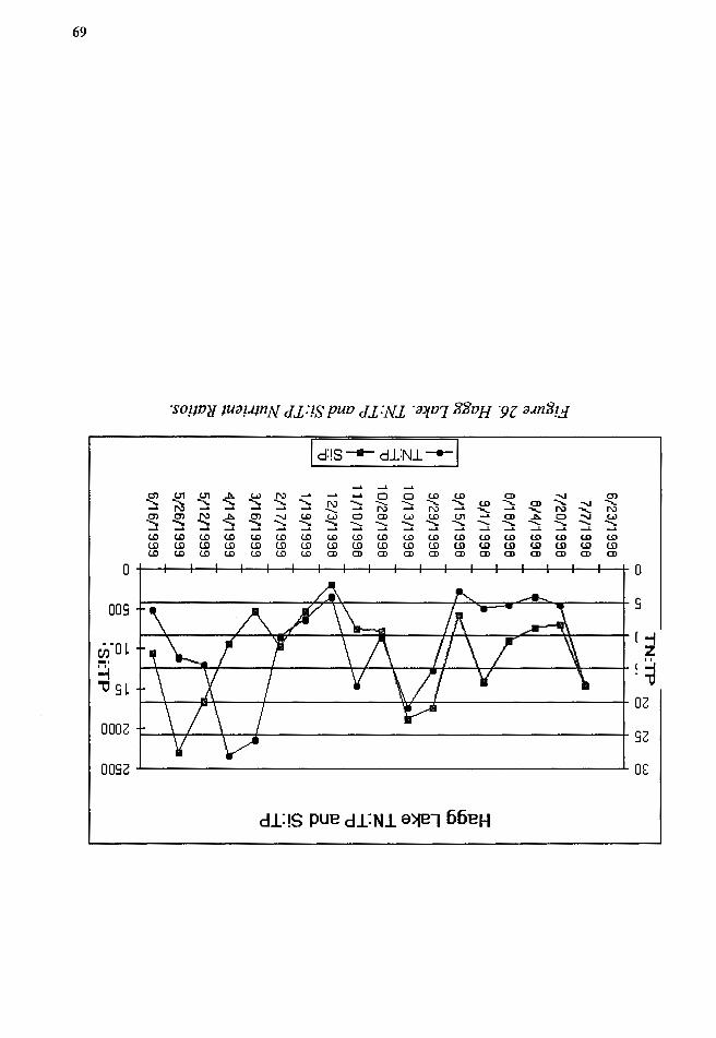
69
I d!S - dJ_NJ_ ---1 ......
0) (;1 (;1 A c...l N ...... ..... a a U) U) CD ...... 0)
-::::. -.... -::::. -::::. -.... -::::. -.... I\) -::::. ...... ...... -.... -.... ~
-.... CD -.... ...... -.... N ...... ...... ...... N ...... N ...... ...... ...._ N ...._ N
0) 0) N A 0) ...... U) c...l C) CD c...l U) (;1 CD A C) ...... c...l ....... ~ ....... ....... ~ ~ ~ ~ ...... -::::. -::::. ~ ~ ...... ~ ...... ~ """" ~ ...... ...... ...... ...... ...... ...... ...... U) U) U) U) U) U) U) U) U) U) U) U) U) U) U) U) U) U) U) CJ) CJ) CJ) CJ) CJ) CJ) CJ) CJ) U) U) U) CJ) CJ) ~ CJ) ~ Ul ~ CJ) U) U) U) U) U) U) U) CD CD CD CD CD CD CD CD CD CD CD CD
0 0
009
1--......... ~~~'---'t;11T--~~+...-=--11t-~~+-+-+-~-::;::>"'-~'tt-~--+(~
z 1--~~___;i~~~~-1--~~~~+-1-----'r~~......,r--~..........,~~~~~-'9r-~~+c ~
- "'O
l--4-~~~~~~~~~~~--J.....,.__---1-~~~~~~~~~-+0Z
0006
c) Biological factors
1. Phytoplankton
Ten species contributed to 95.6% of the total annual biovolumes (Table
4), seven of these formed colonies (including Asterionela formosa and Synedra
radians), and four of them had at times biovolumes that coincided with
smaller peaks in chlorophyll-a (Figure 27). In June 1998 a bloom of Synedra
radians and Fragilaria crotonensis contributed to the higher chlorophyll-a
measurements. This bloom was followed by a bloom of Dinobryon bavaricum
(7 /20/1998). An increase in Cryptomonas sp. biovolumes in the sample of
November 11, 1998 occurred at the same time chlorophyll-a readings were
6.67 µg/L; another Cryptomonas sp. increase in May 1999 corresponded to
12.8 µg/L. An increase in the biovolumes of Chlamydomonas sp. caused the
next highest chlorophyll-a reading (13.1 µg/L).
70

--.l .......
Sa
mp
e I
D
HS
Ol
HS
02
H
S0
3
HS
04
H
S0
5
HS
06
H
S0
7
HS
08
H
S0
9
HS
lO
Da
te
6/23
/98
7171
98
7/20
/98
8/4/
98
8/18
/98
9/1/
98
9/15
/98
9/29
/98
10/1
3/98
10
/28/
98
Ast
erio
ne//a
for
mos
a 20
93.1
06
7720
.135
45
12.7
73
0 64
2.07
23
0 0
2983
9.57
11
4398
.1
2957
.36
Mel
osira
var
ians
31
0.93
67
36.1
2137
0
1578
.842
90
2.53
95
1370
.808
14
79.8
74
4092
.144
18
704.
81
6281
3.8
An
ab
ae
na
flo
s-aq
uae
0 48
1.96
64
4310
4.2
4512
6.35
30
893.
39
7113
.955
57
591.
92
5889
9.78
19
246.
1 17
119.
39
Sph
aero
cist
is s
chro
ete
ri
499.
0332
52
113.
56
8483
.769
25
33. 9
4 25
35.2
23
0 79
1.70
05
8483
.152
67
20.7
63
2223
.361
D
inob
ryon
ser
tula
ria
0 0
3946
.862
62
012.
35
8614
0.3
2158
29
3794
33.8
61
119.
01
0 0
Chl
amyd
omon
as s
p.
0 34
6.03
09
2249
.052
19
8.90
82
8876
.394
26
24.8
57
2658
.51
6674
2.14
48
779.
87
1373
00.7
F
ragi
/aria
cro
tone
nsis
11
3831
6 30
138.
03
0 16
06.3
45
0 21
453.
72
1220
04.2
0
0 14
10.3
78
Cry
p to
mon
as
sp.
0 83
59.6
27
1328
9.94
37
79.2
26
8754
5.29
12
29.8
16
4075
2.04
46
544.
83
5214
3.48
24
5530
.9
Din
obry
on b
avar
icum
51
13.4
12
6425
2.74
32
6007
7 14
6297
.9
1621
8.9
1086
7.17
60
217.
74
4325
.039
0
0 S
yned
ra r
adia
ns
4505
123
9402
.405
85
6.59
6 15
16.3
67
1511
8.62
0
1066
.011
25
79.2
65
301.
6524
49
9.09
08
Sa
mp
e I
D
HS
ll
HS
12
H
S1
3
HS
14
H
S1
5
HS
16
H
S1
7
HS
18
H
S1
9
Dat
e 11
/10/
98
12/3
/98
1/19
/99
2/17
/99
3/16
/99
4/14
/99
5/12
/99
5/26
/99
6/16
/99
Ast
erio
ne//a
for
mos
a 0
342.
911
491.
8943
40
3.61
1 0
0 0
234.
3792
0
Mel
osira
va
ria
ns
8426
8.29
40
006.
26
3180
5.97
32
14.6
5 48
55.9
10
662.
49
6059
.004
34
04.4
1 80
70.3
34
An
ab
ae
na
flo
s-aq
uae
4422
.404
0
0 0
0 0
0 0
0 S
phae
roci
stis
sch
roet
eri
5685
.042
0
0 0
0 0
0 0
3911
60.4
D
inob
ryon
ser
tula
ria
0 15
99.8
4 0
0 0
0 0
546.
7443
0
Chl
amyd
omon
as s
p.
8164
9.66
38
28.2
74
1608
2.34
15
556.
19
8355
7.26
24
4981
.1
9774
6.18
74
13.7
59
0 F
ragi
laria
cro
tone
nsis
0
1471
8.15
0
0 0
0 11
56.2
75
3822
6.9
704.
0564
C
rypt
omon
as s
p.
5410
72.2
80
795.
76
1192
10.2
24
453.
7 68
674.
07
1101
08.8
26
3874
.2
3155
.646
0
Din
obry
on b
avar
icum
0
509.
4514
0
0 0
0 0
0 0
Syn
edra
rad
ians
0
520.
825
0 0
0 28
80.2
78
2577
7.8
1376
4.69
0
Tab
le 4
. Dom
inan
t Phy
topl
ankt
on s
peci
es i
n H
agg
Lak
e (µm~ m
l).
----
. --r.,..._---,----~-.-~.---,.--.~~~---~-
-•·-~---·-·-----~·~----
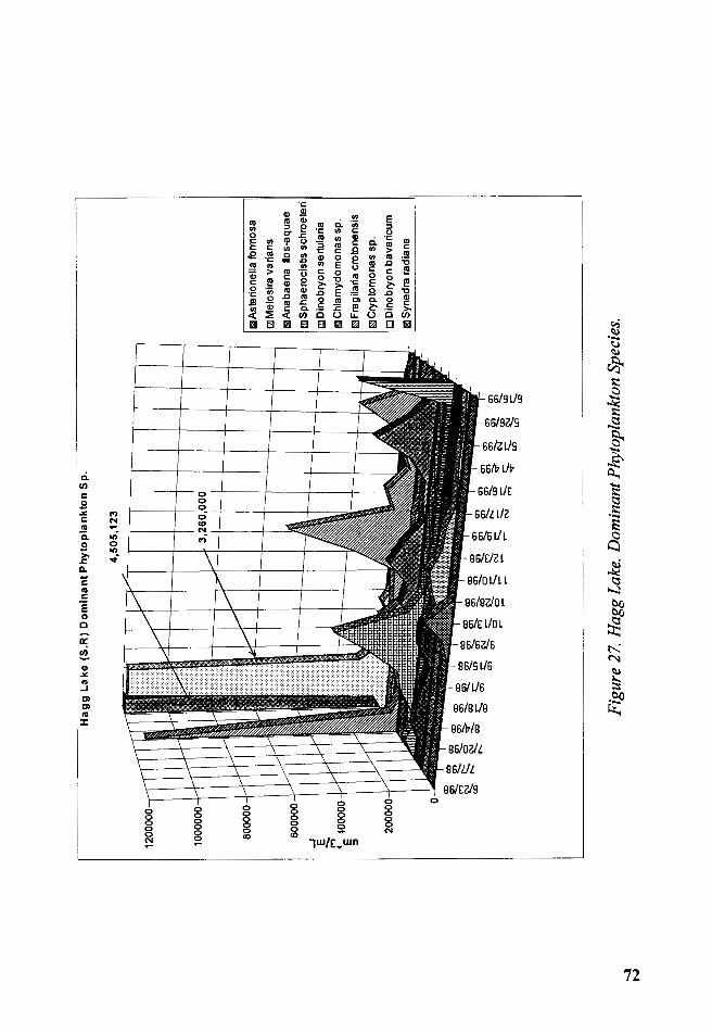
-1
N
1200
000
1000
000
...J ~ <E io
oooo
::J
Ha
gg
La
ke
(S
.R)
Do
min
an
t P
hyto
pla
nkto
n S
p.
4,5
05
, 12
3
3,2
60
,00
0
>:::::.
U>
--~-en-~~
m
01
;;;>
-N"
--
..... '1:::!.cS~,, ~
$
m
O
.......,
, N
-
m
m
$-$-
I:::!.
c "'
«>
ISIA
ster
ione
lla f
orm
osa
lllM
elo
sira
va
ria
ns
111A
naba
ena
flos-
aq
ua
e
Ill S
phae
roci
stis
sch
roet
eri
Ill D
ino
bry
on
ser
tula
ria
1111
Chl
amyd
omon
as s
p.
~ F
ragi
lari
a cr
oto
ne
nsi
s
~Cryptomonas s
p.
o D
ino
bry
on
ba
vari
cum
1111
Syne
dra
rad
ian
s
Fig
ure
27.
Hag
g L
ake.
Dom
inan
t Phy
topl
ankt
on S
peci
es.
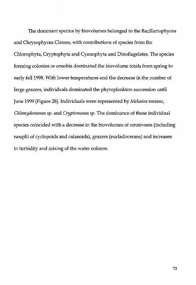
The dominant species by biovolumes belonged to the Bacillariophycea
and Chrysophycea Classes, with contributions of species from the
Chlorophyta, Cryptophyta and Cyanophyta and Dinoflagelates. The species
forming colonies or cenobia dominated the biovolume totals from spring to
early fall 1998. With lower temperatures and the decrease in the number of
large grazers, individuals dominated the phytoplankton succession until
June 1999 (Figure 28). Individuals were represented by Melosira varians,
Chlamydomonas sp. and Cryptomonas sp. The dominance of these individual
species coincided with a decrease in the biovolumes of omnivores (including
nauplii of cyclopoids and calanoids), grazers (eucladocerans) and increases
in turbidity and mixing of the water column.
73

Hagg Lake (S.R.) TotalCobrial w. lnd,,.rual Sp.
:a::o:rm
18IOCO
18lDD
14IDD ----5.fHl!Hi------------------------------------·
1JlllD ..,._ lrdi\id..asl
10IllD ---------------------------! -+-Cdcrias .J
~ amo 1
~ Elm()
4CDIO
JJlID
0 (I) (I) (I) (I) (I) (I) Cl) (/> (/> Cl) (/> Oi
(/> (/> (/> $ $ Cl) (/> (/> Cl) Oi Oi Oi 0) Oi Oi 0) - - - - .- .- ... - - ...
~ ~ <rl' ~ (is O' Of ~ tq- «J' .- .- - - r- .- .- r-Ui m- ~
..... - M' iiS' «s" .- T"' T"" T""
Figure 28. Hagg Lake. Total colonial vs. individual phytoplankton species.
2. Zooplankton
Five species of organisms, including calanoid and cyclopoid nauplii,
dominated the total zooplankton biovolumes in Hagg Lake (Figure 29 and
Table 4). The phyla and classes encountered were protozoans, eucladocerans,
calanoids, cyclopoids and rotifers. They were grouped according to their
feeding habits: raptorials, filter feeders, omnivores (including the nauplii in
74
the omnivores group) and grazers. In the spring of 1998 and 1999 raptorial
zooplankton and its cohort of nauplii and copepodites dominated the
succession of zooplankton. During the summer 1998, fall 1998 and winter
1999 the filter feeders, grazers and omnivores (non-predators) had lower
biovolumes when compared to predatory zooplankton.
75
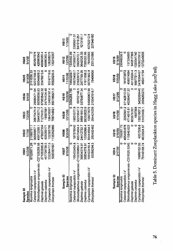
-...!
Q'-.
Sam
ple
ID
HS0
1 H
S02
HS0
3 H
S04
HSO
S H
S06
S[!
ecie
s 6/
23/9
8 7/
7/98
7/
20/9
8 8/
4/98
8/
18/9
8 9/
1/98
B
osm
ina
long
irost
ris
8702
6871
.26
2106
8791
.1
0 0
2111
536.
33
0 C
alan
oid
cope
podi
ds 1
-V
0 36
5688
67.1
20
6754
74.9
29
9864
71.0
4 62
2373
98.8
46
2987
978
Ski
stod
iapt
omus
ore
goni
ensi
s -C
2712
5258
.58
4597
2290
.1
3544
3671
.2
5535
9638
.83
6934
8809
.2
4209
0364
2 D
aphn
ia g
a:ea
ta
2712
5258
5.8
4780
0733
4 71
2791
51. 7
67
9638
42.3
2 33
4760
13.6
45
0903
60.4
D
aphn
ia c
ataw
ba
4577
3873
8.5
6050
8917
1 18
9876
81
2471
4124
.48
0 45
0903
60.4
C
yc/o
poid
s co
pepo
dids
1-V
33
2284
417.
5 10
2385
795
1064
3650
1 12
4559
187.
4 15
7477
19.6
12
6268
079
Dia
cycl
ops
thom
asi
5063
3816
01
1135
3628
60
7687
4992
1 56
0186
821.
5 55
8292
35.9
12
0212
257
Sam
ple
ID
HS0
7 H
S08
HS0
9 H
S10
HS1
1 H
S12
HS1
3 S
[!ec
ies
9/15
/98
9/29
/98
10/1
3/98
10
/28/
98
11/1
0/98
12
/3/9
8 1/
19/9
9 B
osm
ina
long
irost
ris
0 0
0 30
9428
8. 7
56
1965
3209
.7
1335
592.
99
0 C
alan
oid
cope
podi
ds 1
-V
1954
3246
4.8
1879
7804
2 19
8315
77. 9
0
1667
5450
.7
4759
5677
.4
3396
851.
07
Ski
stod
iapt
omus
ore
goni
ensi
s-C
1023
6986
4.7
4557
0434
.4
3021
9547
.3
6976
2146
.5
2382
2072
.4
Dap
hnia
ga/
eata
36
8343
78.9
1 24
4127
32.7
56
6616
51.2
33
7558
77.3
4 29
7775
9.05
D
aphn
ia c
ataw
ba
3683
4378
.91
1220
6366
.4
2833
0825
.6
0 11
9110
36.2
C
yc/o
poid
s co
pepo
dids
1-V
19
5422
418.
4 85
4445
64.5
10
9073
679
6498
0063
.88
6670
1802
.8
Dia
cycl
ops
thom
asi
9305
8294
.5
Sam
ple
ID
HS1
4 S
pec
ies
2/17
/99
Bos
min
a lo
ngiro
stris
0
Cal
anoi
d co
pepo
dids
1-V
O
S
kist
odia
ptom
us o
rego
nien
sis
-C21
1525
.524
3 D
aphn
ia g
alea
ta
O
Dap
hnia
cat
awba
O
C
yclo
poid
s co
pepo
dids
1-V
19
9891
62.0
5 D
iacy
clop
s th
omas
i 76
1491
88.7
4
2604
0248
2
HS
15
3/16
/99
1592
87.7
3 40
5459
.676
11
5845
.622
0 0 42
5732
6.6
4633
824.
87
2644
2103
9 27
0047
018.
7
HS1
6 H
S17
4/14
/99
5/12
/99
0 0
2250
301.
2 91
1428
10.0
3 47
1491
6.81
46
2954
27.2
2 80
3679
.001
0
1607
358
0 13
5018
07.2
34
3320
9446
51
4354
56.1
26
0420
0270
7940
6908
HS1
8 5/
26/9
9 0
1910
7287
2 45
8574
894
4913
3024
.4
9007
7211
.3
2476
3044
27
4804
1179
4
3302
5572
.1
6470
19.2
51
3642
526.
33
1213
161.
1 72
8505
2.66
0
7649
3053
40
7622
12.8
23
3121
685
HS1
9 6/
16/9
9 29
0489
38.3
0 13
7324
003
9408
1736
5 10
2004
1742
16
3603
3912
13
7324
0035
2070
4616
0
Tab
le 5
. D
omin
ant Z
oopl
ankt
on s
peci
es i
n H
agg
Lak
e (µ
mo/
ml).

-...)
-.
..)
5000
0000
00
4500
0000
00
4000
0000
00
3500
0000
00
-g 00
0000
000
- fl 50000
0000
E
:::J
.. 00
0000
000
1500
0000
00
1000
0000
00
Ha
gg
Lak
e D
om
ina
ntZ
oo
pla
nk
ton
--
...,,
C')
.....
..... ~
~~
C')
--~
_ ~
m ~
to
to
::a-cn
-~S23-
~i::::
.;:;:-
;-i:::
:.~~
~
i::::.
N
----
... L
O
LO
C')
~
to
i::::.
to
• B
osm
ina
long
irost
ris
D C
alan
oid
cop
e p
od
ids
1-V
• S
kist
od
iap
tom
us
ore
go
nie
nsi
s
o D
aphn
ia g
ale
ata
m Da
phni
a ca
taw
ba
oC
yclo
po
ids
cop
ep
od
ids
1-V
m Di
a cy
clo
ps
thom
asi
Fig
ure
29.
Hag
g L
ake.
Dom
inan
t Zoo
plan
kton
Spe
cies
.
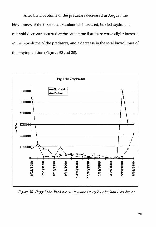
After the biovolume of the predators decreased in August, the
biovolumes of the filter-feeders calanoids increased, but fell again. The
calanoid decrease occurred at the same time that there was a slight increase
in the biovolume of the predators, and a decrease in the total biovolumes of
the phytoplankton (Figures 30 and 28).
1-b]] l..d<e Za:pml<lm
nn I ,--N:mPredax:r_t-------------------,ll"----*-Aedms
fil((((l])-tt--------------------------t-t---
40JDIO))++--------------------+--+--
..J
~ rnm:m (
E :I
:ITQlllID+--+------------------------1----
10lilDJ)J-Mr'"---.-"""<"'7------------------+---+--
0 co (I) (I) (I) co co (I) (!) 0) 0) Cl) Cl) 0) 0) (!) (!) Cl) Cl) 0) 0) 0) O> Q) Q) 0) 0) 0) 0) Q) Q) ... ... .,.. .,.. ... ... ... ... .,.. .,..
~ ~ (i}' i2t (:)- er OJ' ~ ~ i3" ..- ..- ..- ..- ..- ..- ..- ..-Cr (;) Cs ...... - ~ Mi (0 I"" I""
I"" I""
Figure 30. Hagg Lake. Predator vs. Non-predatory Zooplankton Biovolumes.
78
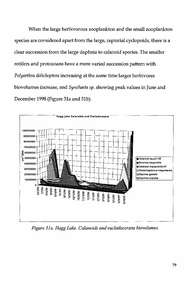
When the large herbivorous zooplankton and the small zooplankton
species are considered apart from the large, raptorial cyclopoids, there is a
clear succession from the large daphnia to calanoid species. The smaller
rotifers and protozoans have a more varied succession pattern with
Polyarthra dolichoptera increasing at the same time larger herbivores
biovolumes increase, and Synchaeta sp. showing peak values in June and
December 1998 (Figure 31a and 31b).
Hagg Lake Calanoids and Eucladocerans
1000000000
900000000
800000000
700000000
...J E iOOOOOOOO ;:;-'e iOOOOOOOO ::I
400000000
300000000
200000000
100000000
0 1 1 1 r , i
~~~~~~~~~ £1~~~~~~~~ w ~ m m m o
' I
- i !S $ $ <::. <::. - <::. ~ z:::. NM;r--LnLnC.D
•Calanoid nauplii I-VI
• Bosmina longirostris
Ill Ca la no id copepodids 1-V
oSkistodiaptomus oregoniensis
aDaphnia galeata
Ill Oaptviia catawba
Figure 31 a. Hagg Lake. Calanoids and eucladocerans biovolumes.
79
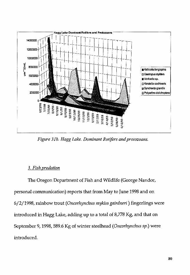
14CXXXXXl
1mmJ
1roxxXX>
...J
~ roxxm Pl < E :3 roxxXX>
Hagg Lake Dominant Rotifers and Protozoans
• t<ellicotia lorgispina
El C:Sstropu; slyliE!s
• Vor1icella sp.
o t<era1ella cocHearis
iil Syn:haeta grardis
o Polyar1tra dolicrop1era
CDCDCD[ [ -
~°'~1ll1llgicoCDCDCDCDa> I [ ~~c~~-~~~~~-~~mm ••• ~~~~,~~~~~~Q·~~~~~~ co "'"'C3°C3';:-~S-~s.cci:::!.~
~ ~ ~ ,. • v "' "' '°'
Figure 31 b. Hagg Lake. Dominant Rotifers and protozoans.
3. Fish predation
The Oregon Department of Fish and Wildlife (George Nandor,
personal communication) reports that from May to June 1998 and on
6/2/1998, rainbow trout (Oncorhynchus mykiss gairdneri) fingerlings were
introduced in Hagg Lake, adding up to a total of 8,778 Kg, and that on
September 9, 1998, 589.6 Kg of winter steelhead (Oncorhynchus sp.) were
introduced.
80

In 1999, from January to March 1998 5,100 Kg of steelhead fingerlings
were liberated in Hagg Lake. From May to June 1999 and on 6/1/1999, 9,908
Kg of rainbow trout fingerlings were introduced in Hagg Lake.
The impact of fish on the zooplankton and phytoplankton was not
measured directly. However, I infer that when fish are small in size, they will
feed on some of the larger zooplankton Gune 1998, September 1998 and May
1999 declines of larger zooplankton), and in turn the disappearance of the
larger zooplankton will allow smaller zooplankton to thrive (Stewart, 1980),
(Figure 29).
4. Species diversity
In this study, the Shannon-Weiner index of diversity was used to
measure the information content of the samples. The Shannon-Weiner index
is used here to explore the diversity-stability relationships, with the
understanding that diversity is an aspect of the community and stability is
an aspect of the community functions (Washington, 1984). The Shannon-
Weiner function described by:
s s
H' = - L:[(p;)·(Log2p;)] or H' = - L:[(p; ·Ln(p;))! Ln(2)] (formula 1.0) i=l i=l
Were s= number of species, pi= proportion of that species over the
total value in a sample (Washington, 1984).
81

Reynolds (1984) suggested that diversity indices using biovolumes
instead of cell counts could be more sensitive to changes in dominance. Thus,
in this thesis, p; = proportion of the biovolume of the species i over the total
biovolume in a sample.
The calculated values of this index, for zooplankton and
phytoplankton in Hagg Lake, are given in Figure 32a. The average diversity
measured was 1.77 bits per individual for the zooplankton and 1.80 for the
phytoplankton.
The graph shows that the Shannon-Weiner index for the
phytoplankton decreased at the same time dominance of one or two species
(Dinobryon sp., Synedra radians) occurred, and increased as these species
ceased to dominate and were replaced by smaller and non-colonial forms
(Fall of 1998).
The zooplankton index followed a different trend with increases in its
value as the summer and fall contribution of smaller bodied zooplankton
increased. The diversity index value declined during the winter as the
biovolume contribution of the species decreased and high inflows, wind
mixing, high turbidity and low temperatures occurred.
The normalized evenness or redundancy with a range of 0 to 1.0 was
calculated as well, with 1 indicating even samples (many co-dominant
species). In Hagg Lake, the average value of evenness was 0.27 for
82
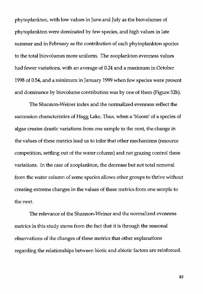
phytoplankton, with low values in June and July as the biovolumes of
phytoplankton were dominated by few species, and high values in late
summer and in February as the contribution of each phytoplankton species
to the total biovolumes more uniform. The zooplankton evenness values
had fewer variations, with an average of 0.24 and a maximum in October
1998 of 0.54, and a minimum in January 1999 when few species were present
and dominance by biovolume contribution was by one of them (Figure 32b).
The Shannon-Weiner index and the normalized evenness reflect the
succession characteristics of Hagg Lake. Thus, when a 'bloom' of a species of
algae creates drastic variations from one sample to the next, the change in
the values of these metrics lead us to infer that other mechanisms (resource
competition, settling out of the water column) and not grazing control these
variations. In the case of zooplankton, the decrease but not total removal
from the water column of some species allows other groups to thrive without
creating extreme changes in the values of these metrics from one sample to
the next.
The relevance of the Shannon-Weiner and the normalized evenness
metrics in this study stems from the fact that it is through the seasonal
observations of the changes of these metrics that other explanations
regarding the relationships between biotic and abiotic factors are reinforced.
83
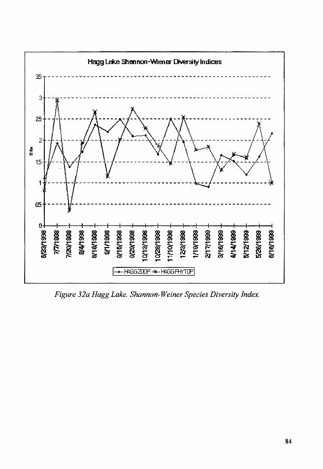
Ji8
--------------------------------------------------------~
--------------------------------------------------------£
---------------------------------------------------------S'£
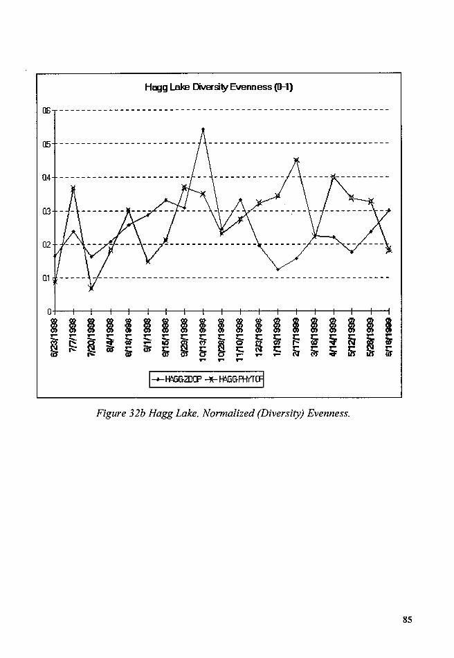
S8
-------------------------90
------------------------------------------------------------so

2. BARNEY RESERVOIR
In this section the physical, chemical and biological factors that were
measured during the sampling period are described and analyzed. Table 9a
and 9b list a summary of descriptive statistics for Barney Reservoir data.
Microphotographs of selected specimens of the plankton are presented in
figure 61.
a) Physical Factors
1. Water Inflows and Outflows
Barney Reservoir inflows were not measured but observations
indicated that the sources of inflows is varied and that the contribution of
small streams reaching the reservoir might be equal or greater than the
contributions of the North fork of the Trask River (Figure 33).
The data on the water outflows comes from weekly monitoring
reports of the dam operation prepared by the operators at the Forest Grove
Water Treatment Plant.
The reservoir, as operated during the study period, had extreme
changes in storage volumes (Table 1). It reached a maximum water surface
elevation of 497.9 ma. m. s. l., and a minimum elevation of 479.1 ma. m. s. l.
The difference between maximum and minimum elevation was 18.8 m. The
86
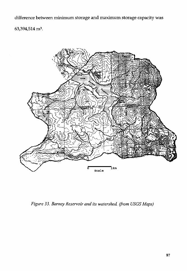
difference between minimum storage and maximum storage capacity was
63,394,514 m3.
Figure 33. Barney Reservoir and its watershed (from USGS Maps)
87
Due to lack of precipitation data from Barney Reservoir, the
precipitation data from Hagg Lake was used as a proxy to help explain the
changes in water levels, storage and outflow regime of Barney Reservoir.
The changes in water elevation can be described as follows: from May
to June 1998, the water levels remained at a stable elevation (492 ma. m. s. l.),
and releases were relatively small (65,504 m3 /Day). From June to the end of
October 1998, the water elevation decreased steadily to 480 m a.m.s.l.
From November First to December 15, 1998 as precipitation increased
and outflows remained unchanged, the water levels rose 10 min this period.
By the end of the winter the water level had reached a high of 497.9 ma. m. s.
1. (3/1/1999). In consequence the outflows were increased to 440,383
m3/Day. Decreases in precipitation in April 1999 resulted in a sharp decrease
in the outflows (19,572 m3/Day) to keep the water levels at around 490 m.
a.m.s.l. until June 1999 (Figure 34a).
88
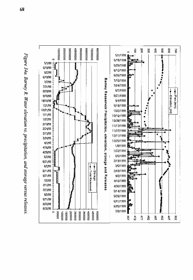
68
5/1/98
5/18/98
6/2198
6/18/98
7/7/98
7/31/98
8/28/98
9/18/98
10/19/98
12/1/98 12/21/98
l/11/99
1/27/99
2/10/99 2/24/99
3/13/99
3/24/99
4/7/99 4/16/99
4/28/99
5/7/99
5/21/99 6/2199
6/11/99
6/21/99
7/2/99
7/12/99
7/23/99
8/2/99
8/11/99
8/20/99
N w .i:.. <.n m .....,. ca g g g g g g g g 0 0 0 0 0 0 0 0 0 0 0 0 0 0 0 0 0 0 0 0 0 0 0 0 0 0 0 0 0 0 0 0
0 0 0 0 0 0 0 0 0
t t -l en 0 -lit ~ - .. ;u cc CD CD
CD" .. "' CD c.
8/30/99 +---J-"L-+-'-+-'"-'-+---+---+'--+-'-1----'-f-----j 0 <.n N N W W .i:.. .i:.. <.n
0 0 <.n 0 <.n 0 <.n 0 <.n 0 0 0 0 0 0 0 0 0 0 0 0 0 0 0 0 0 0 0 0 0 0 0 0 0 0 0 0 0 0 0
0 0 0 0 0 0 0 0 0
Ill DI ... :I CD '< :;o CD Ill Ill CD
<! 0 ::;· -a iii 0 -s· ;::;: DI -c;· :I
CD iD" ~ -c;· 3 Ill -0 iil IC
CD
DI :I c. :;o CD iD" DI Ill CD Ill
N
0 8 "' 0 0 "" 0
0 "' m 8 8
..... 0 0
5/1/1998 lil=:z.-t--t------t--+--+--+------1
5/15/1998 -~Piii=f~ 5/29/1998
6/12/1998
6/26/1998
7/10/1998
7/24/1998
8/7/1998
8/21/1998
9/4/1998
9/18/1998 li==AP--o • •
10/2/1998 ~~3~ : 10/16/1998 •
• • •
t • • t t m -c CD CD < 0 "' ;.... "" 3 g 3 I ~
3 e
10/30/1998 ~~... •
11/13/1998 liiiE~~=f.1~t 11/27/1998
12/11/1998 ••
12/25/1998 1"':;:+.=~--r..-+-1~. _, 1/8/1999 •
2/5/1999 ~i==i~t1 2/19/1999 ~~~~~~-1-3/5/1999 Ii
3/19/1999 4/2/1999 u~~-
4/16/1999
4/30/1999
5/14/1999
5/28/1999
6/11/1999
6/25/1999
7/9/1999 v---~r--+~-+-~+---;~-+----1
"" ..... N "" CX>
N "" "" CX> <D -..i N "" "' <D 0
-..i N
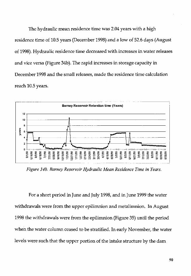
The hydraulic mean residence time was 2.04 years with a high
residence time of 10.5 years (December 1998) and a low of 52.6 days (August
of 1998). Hydraulic residence time decreased with increases in water releases
and vice versa (Figure 34b). The rapid increases in storage capacity in
December 1998 and the small releases, made the residence time calculation
reach 10.5 years.
Barney Reservoir Retention time (Years)
12~~~~~~~~~~~~~~~~~~~~~~~~~~~~~~~~~~~~~~~-
10 +--~~~~~~~~~~~+-~~~~~~~~~~~~~~~~~~~~~~~~~~-
8 +-~~~~~~~~~~--Jc+-~~~~~~~~~~~~~~~~~~~~~~~~~~-
"' ii 6 I I I ~ lr-t u~ t 4+------1~--~~~~~~-+-+~~~~~~~~~~-+-~~~-+-+">--~~~~~~~~-
: l11111111111~''"'~111S::::1nmmrmmmfttt11111111111111~1:=::::::::::::::::::::: ro ro ro ro ro oo oo oo oo ro ro m m m m m m m m m m m m m m m m m m m m m ~~~~~~~~~~~~~~~~~~~~~~~~~~~~~~~~ c 00 ~ 00 ~ - 00 00 m - - - ~ 0 v M v ~ w ro ~ - ~ - - ~ N M ~ - 0 0 ~cwc~~~cc~~c~c~c~~c~~~wc~~c~roc~~
~ W ~ 00 m 0 - N - - N N M M V V W W W ~ ~ 00 00 00
Figure 34b. Barney Reservoir Hydraulic Mean Residence Time in Years.
For a short period in June and July 1998, and in June 1999 the water
withdrawals were from the upper epilimnion and metalimnion. In August
1998 the withdrawals were from the epilimnion (Figure 35) until the period
when the water column ceased to be stratified. In early November, the water
levels were such that the upper portion of the intake structure by the dam
90
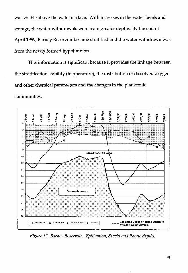
was visible above the water surface. With increases in the water levels and
storage, the water withdrawals were from greater depths. By the end of
April 1999, Barney Reservoir became stratified and the water withdrawn was
from the newly formed hypolimnion.
This information is significant because it provides the linkage between
the stratification stability (temperature), the distribution of dissolved oxygen
and other chemical parameters and the changes in the planktonic
communities.
.. .. " "' "' c.. tl
.. "' "' "' "' "' "' "' "S "S " " c.. "' "' .... .... "' "' "' "' "' ... ...
" tl ~ .... 0 .... .... ..... .... ..... ~ ~ 7 7 7 ~ ~ "' c.;i 9 :::::. :::::. "" "" "' ... "' Cll 0 :::::. N N N
~ .... ....
0 .. "' ... "' .0 N I 0 ... ... "" ~ ;;;- ~ i'il" ;:::-"" ... N ... N N "' N ... - - -0
10 ~ 1' I =z'.'.t~ :' \ I I 12 I'\. f 7~
14 +-----------#'
16 +---------'
1 B +-------"
20 +----....,.
22
24
26
28 f : ::: -<::: ::::::>·· .. .-: ::-: ·. :·:-. ·-: .· . . . . : ::: :::: :::~ : :::::: : : ::: ::: ::: :::::::::::::::! -+-0 eplh (m I --o-E pi· de plh -.-Pho tic Zone -o-S ecchi __ Estimated Depth or Intake structure
from the Water Surface.
Figure 35. Barney Reservoir. Epilimnion, Secchi and Photic depths.
91
2. Temperature
From spring to the mid-fall 1998, Barney Reservoir was stratified. At
the same time, as the water elevation dropped, the water column began to
mix (Figure 35). However, these lower water levels alone do not explain the
early mixing of the water column. The general West-to East orientation of the
surrounding hills force the westerly winds to increase their velocities by a
'canyon effect' and to transfer some of their energy to the surface water of the
reservoir. Since the main axis of reservoir (fetch) is also oriented in the same
general direction of the hills the resulting effect is a mixed water column. As
a result, from early September 1998 to April 1999 this reservoir had a mixed
water column (Figure 36).
The epilimnetic temperature had an average value of 13. 9° C, a high of
26.1° C in July 28, 1999, and a low of 5.8° C in February 1999. The time-depth
graph of the temperature (Figure 36a) shows the extent of the stratification
and the changes in depth at the main sampling station.
The changes in the water elevation of Barney Reservoir and the
changes in the depth from the water surface of the intake structure had an
impact on the metalimnion and hypolimnion. This impact was in the form of
increased hypolimnetic temperatures, which ranged from 9.1° C in July 1998
to 18.2° C at the end of stratification.
92
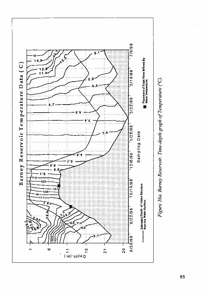
\C
w
6
E 1
1
.c::. ... a.
Q)
0 1
6
21
26
6/3
Barn
ey
Reserv
oir
Tem
pera
ture
Data
( C
)
Est
imat
ed D
ep
th o
f In
take
Str
uct
ure
fr
om th
e W
ater
Sur
face
.
Sa
m p
iin
g D
ate
•
Pla
cem
ent o
f Tra
sk R
ive
r In
flo
ws
By
Wat
er T
empe
ratu
re.
Fig
ure
36a.
Bar
ney
Res
ervo
ir.
Tim
e-de
pth
grap
h o
f Tem
pera
ture
(°C
).
-~---_._,_,_,_·---~--
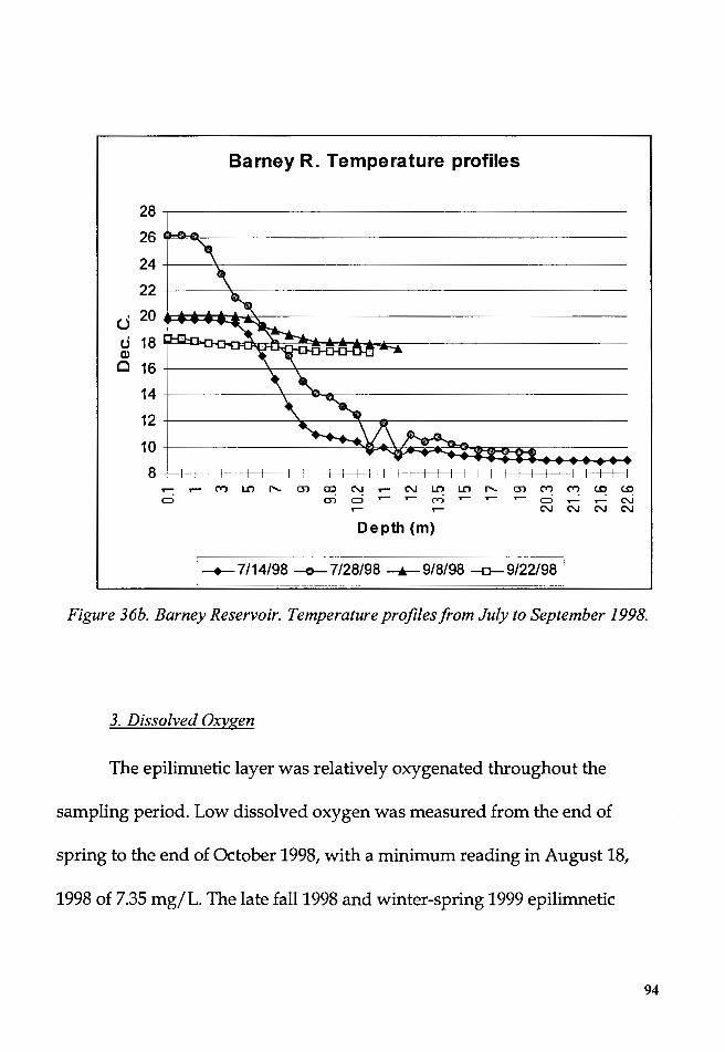
Barney R. Temperature profiles
28~--------------------26a,,e.a_ __________________ _
24_[_-~------------------
22-"---~--------------------
~ ~~ ~····~~----------Q)
0 16j__---~-----4---------------
14_[_-----4-------8---------------
12-"------~-.--~--------------
1~ I 1 I I I I I I I I I I I : =~~!!!!! t t t t t t ~ ~ ~ M ~ ~ m w N ~ N ~ ~ ~ m M M ~ ~
ci m 0 ~ ~ ~ ~ ~ ~ ci ~ ~ N N N N N
Depth (m)
I-+-7/14/98 -e- 7/28/98 __.__918/98 --o-9/221981
Figure 36b. Barney Reservoir. Temperature profiles from July to September 1998.
3. Dissolved Oxygen
The epilimnetic layer was relatively oxygenated throughout the
sampling period. Low dissolved oxygen was measured from the end of
spring to the end of October 1998, with a minimum reading in August 18,
1998 of 7.35 mg/L. The late fall 1998 and winter-spring 1999 epilimnetic
94

dissolved oxygen concentrations were higher with the maximum
concentration measured on January 12, 1999at13.3 mg/L.
During the stratification of the summer 1998, anoxia conditions
formed in the hypolimnion. Some decomposition of organic material could
be responsible for this depletion of dissolved oxygen; this explanation is
supported in part by the pH values (Figure 40). However, another plausible
explanation for the anoxic conditions in the hypolimnion is that increases in
water temperatures related to falling water levels, could cause losses of
dissolved oxygen to the atmosphere. As the solubility of oxygen depends on
water temperature, atmospheric pressure and ionic concentrations, generally
at higher water temperatures, the dissolved oxygen saturation values
diminish (Wetzel and Likens, 1991).
The profiles of dissolved oxygen appeared less influenced by the
changes in the depth from the water surface of the intake structure, as was
the case in Hagg Lake.
95
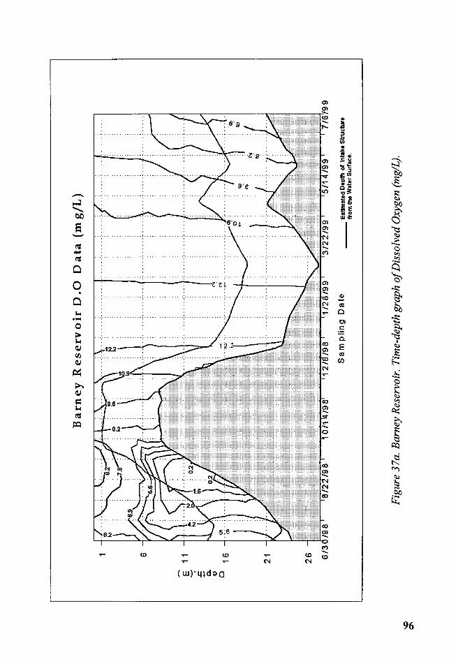
\C
Q'\
6
E
11
.s::. - 0.. Q,) D
16
21
26
6/3
Barn
ey
Reserv
oir
D.O
Data
(m
g/L
)
"" ..., "'
N
....
....
....
....
....
....
.
Sa
m p
iin
g D
ate
E
stim
ated
Dep
th o
f In
take
Str
uct
ure
---
fro
m th
e W
ater
Sur
face
.
Fig
ure
3 7 a
. B
arne
y R
eser
voir
. T
ime-
dept
h gr
aph
of D
isso
lved
Oxy
gen
(mg!
L).
--"···---~----·--· ~---
----
··--
·-··
--

\,/;;
......
)
Bar
ney
Res
erv
oir
D
isso
lved
Ox
yg
en (
Per
cen
tag
e S
atu
rati
on
)
1 6
11
E
._. =
a.
Q)
0 1
6
21
26
6/3
0/9
8
8/4
/98
9
/8/9
8
10
/14
/98
11
/18
/98
12
/24
/98
1/2
8/9
9
3/4
/99
4
/9/9
9
5/1
4/9
9
6/1
9/9
9
7/1
7/9
8
8/2
2/9
8
9/2
6/9
8 1
0/3
1/9
8 1
2/6
/98
1
/10
/99
2
/15
/99
3
/22
/99
4
/27
/99
6
/1/9
9
7/6
/99
E
stim
ated
De
pth
of
Inta
ke S
tru
ctu
re
---
fro
m th
e W
ater
Sur
face
. S
am
plin
g D
ates
Fig
ure
3 7b
. B
arne
y R.
Tim
e-de
pth
grap
h o
f Dis
solv
ed O
xyge
n (%
Sat
).

4. Secchi depth and lrradiance:
Barney Reservoir average Secchi depth was 3.14 m. The Secchi depth
was higher during the spring and early summer of 1998 (average 4 m) and
lower during fall 1998 and winter 1999 (average 2 m). In 1998 the highest
Secchi depth was measured at 4.75 m on June 30. The 1999 highest Secchi
depth was measured in April at 4.9 m. The lowest Secchi depth was
measured in October 1998at1.75 m (Figure 38). Secchi depth appeared to be
more affected by changes in the water levels than by the high inflows caused
by the late fall and winter storms. However, high inflows also decreased
water transparency (i.e. Secchi depth of 2 min February 1999).
98

Barney Reservoir __. -'
01 - ........ ..... ............
(3") ........ - ....._ w N
CD (0 a ..... __. w - ....._ -...... ""' ....._ -N N l\J -' - N
Cl OJ 01 l\J a ~ l\J w w -..J ...._ "'- ...._ "'- -...... ""' "'- ...._ ...._ -...... -' __. -' __. __. -' __. -' -' -m (.0 m (.0 <.Q <.Q (.0 m m <.Q w (D w (0 (0 w (0 w w (D
CD OJ CD OJ OJ CD (.Q m m (.Q
0 0
1 5
2
3 10
15 ~ z
~ 4 ... E 5
6 20
7 25
8
9 30
I-¢- Secchi ____,,__ Eupho1icZore __.___ NTU_Turb I Figure 38. Barney Reservoir. Secchi and Photic depth.
Irradiance (µEinsteins m-2 ·s-1) was used to calculate the depth of the
photic zone (Wetzel, 1991). The pattern that emerged was somewhat similar
to the Secchi depth, with the shallowest photic zone occurring in September
1998 at 2.86 m, and the deepest photic zone in June 1998 at 7.25 m and July
99
1999 at 7.76 m. The photic zone was deeper during the spring and early
summer of 1998 and the spring of 1999. As with Secchi depth, the depth of
the photic zone was influenced by the biovolumes of plankton, the low water
levels, the short, unstable stratification period and the greater winter inflows
of water.
5. Turbidity
Epilimnetic turbidity in Barney Reservoir was relatively low, with a
minimum value of 4 NTUs in May 1999 and a maximum value of 28 NTUs in
August 1998. Increases in turbidity in Barney Reservoir during the spring
and fall of 1998 were related to low water levels, and to increased water
inputs during winter 1999. The turbidity throughout the water column
during all the sampling dates was relatively homogeneous, except in the
sample that coincided with the maximum drop in the water levels (Figure
38). An explanation offered is that as the water levels fell, sediments from the
coves and shores were disturbed by the waves and carried back to the
pelagic waters. When the water levels ceased to drop, the sediments sank
and the turbidity values decreased (Figure 39). The overall relatively low
observed turbidity could be the result of a combination of factors such as a
smaller watershed with a high percentage covered by vegetation, low human
impacts, and many sources of low volume inflows (Table 1, Figure 33).
100
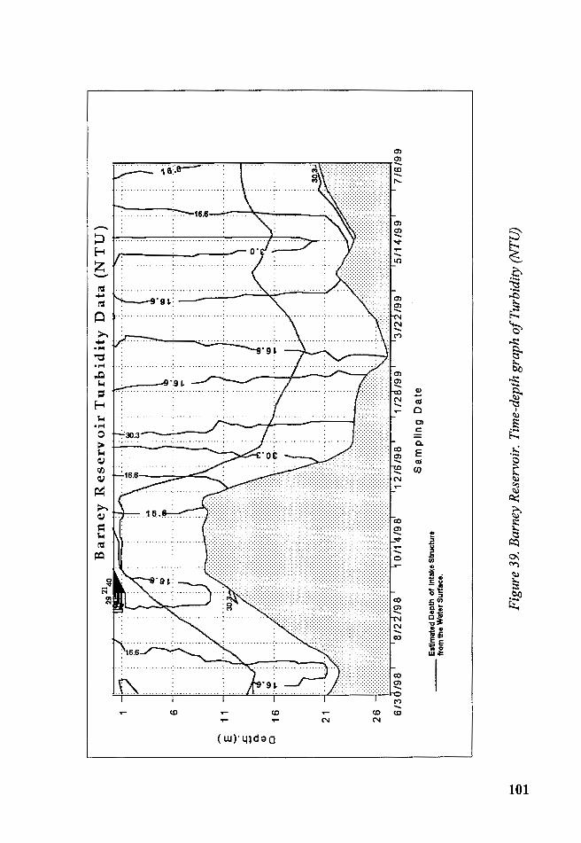
.... = ....
---~--
·-~·
6
E
11
.c
0.
Cl)
0 1
6
21
26
'/
Barn
ey
Reserv
oir
Tu
rbid
ity
Data
(N
TU
)
Est
imat
ed D
ep
th o
f In
take
Str
uctu
re
from
the
Wat
er S
urfa
ce .
'.l!j :(.)
":"C
a.
Sa
mp
lin
g D
ate
fO
.· ...
~--:
··
Fig
ure
39.
Bar
ney
Res
ervo
ir.
Tim
e-de
pth
grap
h o
f Tur
bidi
ty (
NTU
}
-: 1
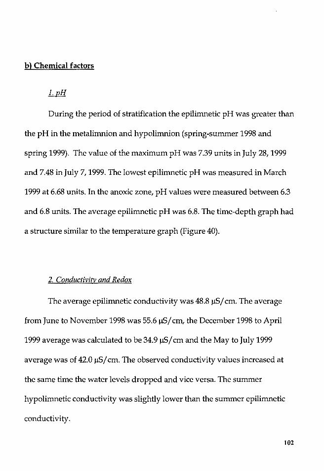
b) Chemical factors
1. pH
During the period of stratification the epilirnnetic pH was greater than
the pH in the metalirnnion and hypolirnnion (spring-summer 1998 and
spring 1999). The value of the maximum pH was 7.39 units in July 28, 1999
and 7.48 in July 7, 1999. The lowest epilirnnetic pH was measured in March
1999 at 6.68 units. In the anoxic zone, pH values were measured between 6.3
and 6.8 units. The average epilirnnetic pH was 6.8. The time-depth graph had
a structure similar to the temperature graph (Figure 40).
2. Conductivity and Redox
The average epilirnnetic conductivity was 48.8 µS/ cm. The average
from June to November 1998 was 55.6 µS/cm, the December 1998 to April
1999 average was calculated to be 34.9 µS/ cm and the May to July 1999
average was of 42.0 µS/ cm. The observed conductivity values increased at
the same time the water levels dropped and vice versa. The summer
hypolirnnetic conductivity was slightly lower than the summer epilirnnetic
conductivity.
102

Unlike in the case of Hagg Lake the depth of the intake structure from
the water surface had no effect on the profiles of conductivity (Figure 41 ).
The epilimnetic redox values (m V) were low during the stratified summer of
1998, and higher when the water column was mixed or the water levels were
high. Hypolimnetic redox values in the summer of 1998 were higher and
conductivity was lower than the epilimnetic values. When the water column
was mixed or the water levels were high, the redox measurements were
homogeneous throughout the water column. The epilimnetic low redox
values coincided with some increases in the ammonium and nitrate+nitrite
nitrogen, as well with the highest epilimnetic and metalimnetic chlorophyll-a
measurements (Figure 42 and 44). The dynamic or pattern of the redox
values in Barney Reservoir during the period of this study seemed
influenced by the elevation of the water levels (depth of the water column),
the temperature and the biological activity occurring in the epilimnion,
particularly during stratified conditions.
103
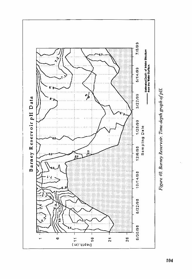
.... Q """
----~--
~.·; --~· --·
1 6
E 1
1
.s::. a.
Cl)
0 1
6
21
26
6/3
0/9
8
8/2
2 /9
8
Barn
ey
Reserv
oir
pH
D
ata
10
/14
/98
1
2/6
/98
1
/28
/99
3
/2 2
/9 9
5
/14
/99
71
619
9
Sa
mp
lin
g D
ate
E
stim
ated
Dep
th o
f In
take
Str
uctu
re
---
fro
m th
e W
ater
Sur
face
.
Fig
ure
40.
Bar
ney
Res
ervo
ir.
Tim
e-de
pth
grap
h o
f pH
----~------~-~----·---~---.--·------·---
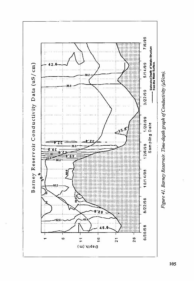
.....
Q u.
6
E
11
.c. .....
0..
11
)
0 1
6
21
26
6/3
0 /9
8
8/2
2/9
8
Barn
ey
Reserv
oir
Co
nd
ucti
vit
y D
ata
(u
S/
cm
)
1 0
/1 4
/98
1
2/6
/98
1
/28
/99
S
am
plin
g D
ate
3
/22
/9 9
:C.1
·U
I : C
o
~
N
5/1
4/9
9
71
61
99
Est
ima
ted
De
pth
of
Inta
ke S
tru
ctu
re
---
fro
m th
e W
ater
Sur
face
.
Fig
ure
41.
Bar
ney
Res
ervo
ir.
Tim
e-de
pth
grap
h o
f Con
duct
ivit
y (µ
Siem
) .
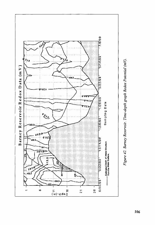
.....
Q
O"I
1 6
e-11
.t::: ~
a.
Q) 01
6
21
26
Ba
rn
ey
Rese
rv
oir
Red
ox
Da
ta (
mV
)
Est
imat
ed D
epth
of
Inta
ke S
tru
ctu
re
from
the
Wat
er S
urfa
ce.
Sa
mp
lin
g D
ate
Fig
ure
42.
Bar
ney
Res
ervo
ir.
Tim
e-de
pth
grap
h R
edox
Pot
enti
al (m
V) .
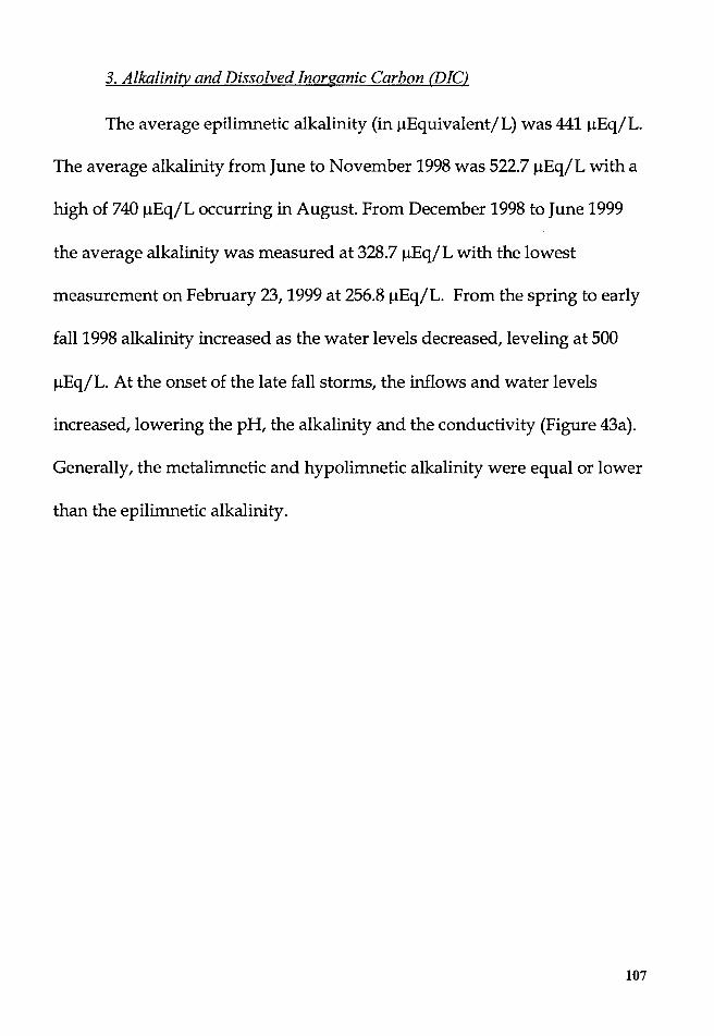
3. Alkalinity and Dissolved Inorganic Carbon (DIC)
The average epilimnetic alkalinity (in µEquivalent/L) was 441 µEq/L.
The average alkalinity from June to November 1998 was 522.7 µEq/L with a
high of 740 µEq/L occurring in August. From December 1998 to June 1999
the average alkalinity was measured at 328.7 µEq/L with the lowest
measurement on February 23, 1999 at 256.8 µEq/L. From the spring to early
fall 1998 alkalinity increased as the water levels decreased, leveling at 500
µEq/L. At the onset of the late fall storms, the inflows and water levels
increased, lowering the pH, the alkalinity and the conductivity (Figure 43a).
Generally, the metalimnetic and hypolimnetic alkalinity were equal or lower
than the epilimnetic alkalinity.
107
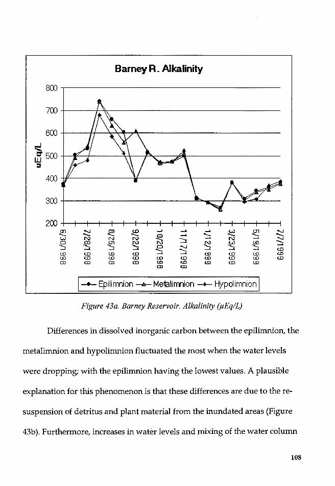
Barney R. Alkalinity
800
700
600 ...J ....... C" 500
LU =
400
300
200 en -....J CD (D -' __. -' w (Jl -....J -o;..J D ...._ -'
...._ - ...._ 0 ....... - ...._ - ...._
N N N ........ - ---' N ---' ---..I co (Jl r\:) N ....... N w U) ............ .....__ ...._ .....__
D -....J ...._ .....__ ...._ ....... __. -' __. - ...._ -' __. -' (D
(£) (.0 (£) (.0 ---' ....... (£) (.0 (£) u::, U) (D U) (D U) (D U) (D U) (.0
CD co CD co '"'° u::, (£) (.0 (£) CD co
I__._ Epilimnion ___._ Meialimnion-+- Hypolimnion I Figure 43a. Barney Reservoir. Alkalinity (µEq/L)
Differences in dissolved inorganic carbon between the epilimnion, the
metalimnion and hypolimnion fluctuated the most when the water levels
were dropping; with the epilimnion having the lowest values. A plausible
explanation for this phenomenon is that these differences are due to the re-
suspension of detritus and plant material from the inundated areas (Figure
43b). Furthermore, increases in water levels and mixing of the water column
108
did not cause increases in the DIC. The average DIC was calculated at 0.139
mg C /Land the highest value calculated at 0.21 mg C / L for the sample of
August 11, 1998. The lowest DIC was calculated for the February 1999
sample at 0.105 mg C/L. The DIC presented here was derived from pH and
alkalinity measurements (Wetzel, 1991).
Barney R. DIC 0.5
0.45
0.4
0.35 ..J 0.3 CJ' 5 0.25
0.2
0.15
0.1
0.05 13) -w C) ....._ -1.
UJ
-...J CD (.0 -1. - - - 0 N N N ........... CD (Tl l'\J r\) ....._ ....._ ....._
C) -1. -1. -1. -UJ UJ UJ -L
--' --' w 01 "'-J ...... - - - -......... ...... N ...... -.J ...... N w (.D -"'-J ...._ ...._ ...._ ...... - _.. --' --' (.D ...... ~ ~ ~ (..,:,
(.0 (.0 (.0 (D (D (.D (.D (.D (.D ~ CD CD CD CD © (..,:, ~ ~ ~
CD co
I--- Epilimnion -m.-Me1alimnion --+-Hypolimrion I Figure 43b. Barney Reservoir. Dissolved Inorganic Carbon (mg CIL).
109
4. Chlorophyll-a
The average epilimnetic chlorophyll-a measurement was 2.1 µg/L.
The highest measurement of chlorophyll-a was 4.53 µg/L made on
September 8, 1998, and the lowest was 0.61 µg/L on December 10, 1998. The
increases in chlorophyll-a did not correlate with a dominant species. The
only observable relationships between increasing chlorophyll-a and
phytoplankton was that all the species contributed to the chlorophyll-a
readings particularly Cryptomonas sp. By biovolumes, Dinobryon sertularia
was the dominant species, however their contribution to chlorophyll-a
measurements was not as proportional. For example, in May 1999 the
biovolumes of Dinobn1on sertularia corresponded to more than 70% of the
total biovolumes but the epilimnetic chlorophyll-a was only measured at 2.98
µg/L (Figure 44). Metalimnetic chlorophyll-a was generally lower than
epilimnetic chlorophyll-a, except in September 8, 1998 when the
metalimnetic chlorophyll a was 9.12 µg/L.
From June to September 1998 chlorophyll-a increased at the same time
water levels decreased and water temperature increased. Once stratification
was lost, chlorophyll-a values from October to November 1998 were between
2.67 and 3.06 µg/L. Cold temperatures increases in the water levels, and low
light condition caused a decrease in chlorophyll-a during the period of
110
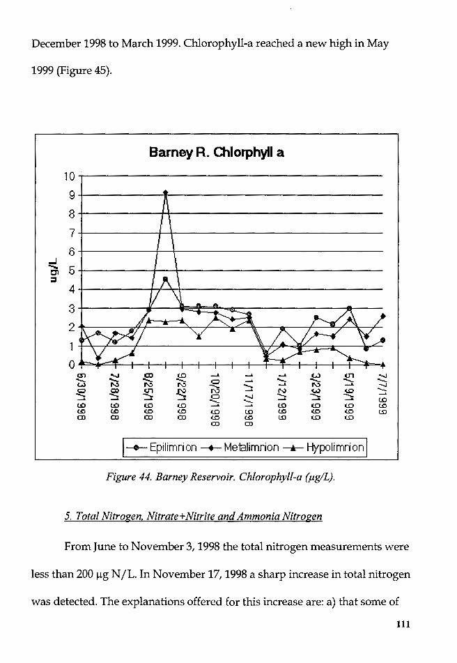
December 1998 to March 1999. Chlorophyll-a reached a new high in May
1999 (Figure 45).
Barney R. 0.lorphyll a
10~~~~~~~~~~~~~~~~~-
9-+-~~~--'lf--~~~~~~~~~~~
s---~~~---1'--~~~~~~~~~~~-
7---~~~-+---~~~~~~~~~~~-
6-+-~~~-+---~~~~~~~~~~~-
~ 5[=-~~-/--;-\-~~~~~~---===== :::i
;! ;&.~A~,) 2 - ..,
0 en "..I (D (.0 __. --' --' w (]1 "..I - - - - 0 ..... - - - -w N N N - ......... --' N __.
-..J Q Q;I "Jl N l'IJ ..... N 'w.:I ~ --::::: ......... ~ ~ a "..I ......... - - ..... ..... - - ..... - - (.0 (.0 (.0 (.0 (.0 - ..... (.0 (.0 (.0 c.,o c.,o U":l 1(1:} 1(1:} (.0 (.0 U":l 1(1:} 1(1:} (£) CD CD (D (D 1(1:} c.,o m (.0 (.0
(D CD
I__.__ Epilimri on --+- Me1alimrion __..._ Hypo Ii mri on I
Figure 44. Barney Reservoir. Chlorophyll-a (µg/L).
5. Total Nitrogen, Nitrate+Nitrite and Ammonia Nitrogen
From June to November 3, 1998 the total nitrogen measurements were
less than 200 µg N/L. In November 17, 1998 a sharp increase in total nitrogen
was detected. The explanations offered for this increase are: a) that some of
111
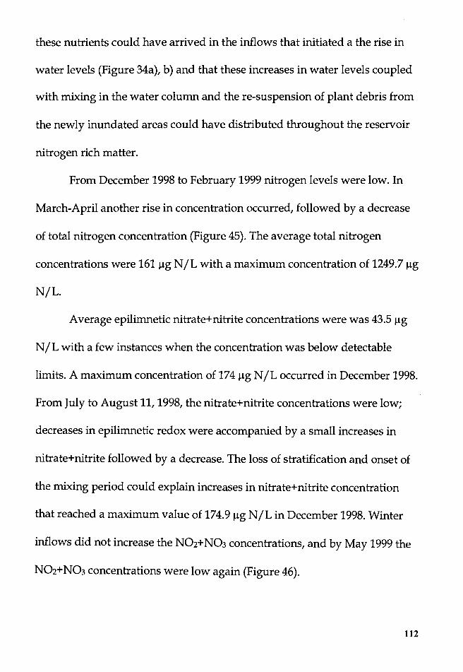
these nutrients could have arrived in the inflows that initiated a the rise in
water levels (Figure 34a), b) and that these increases in water levels coupled
with mixing in the water column and the re-suspension of plant debris from
the newly inundated areas could have distributed throughout the reservoir
nitrogen rich matter.
From December 1998 to February 1999 nitrogen levels were low. In
March-April another rise in concentration occurred, followed by a decrease
of total nitrogen concentration (Figure 45). The average total nitrogen
concentrations were 161 µg N/L with a maximum concentration of 1249.7 µg
N/L.
Average epilimnetic nitrate+nitrite concentrations were was 43.5 µg
N/L with a few instances when the concentration was below detectable
limits. A maximum concentration of 174 µg N/L occurred in December 1998.
From July to August 11, 1998, the nitrate+nitrite concentrations were low;
decreases in epilimnetic redox were accompanied by a small increases in
nitrate+nitrite followed by a decrease. The loss of stratification and onset of
the mixing period could explain increases in nitrate+nitrite concentration
that reached a maximum value of 174.9 µg N/L in December 1998. Winter
inflows did not increase the N02+ N03 concentrations, and by May 1999 the
N02+ N03 concentrations were low again (Figure 46).
112
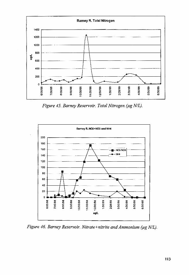
Barney R. Total Nitrogen
1400
1200
1000
800 ~ Cl
" 600
400
200
0 co co co co co co co "' "' "' "' "' "' Q? Q? Q? Q? Q? Q? Q? Q? Q? Q? Q? Q? Q? 0 0 0 0 0 0 0 0 co 0 0 0 0 !'.! !'.! !'.! !'.! !'.! !'.! !'.! !'.! ~ !'.! !'.! !'.! !'.! CD I'- co "' 0 ~ N ~ N "' .... "' CD
~
Figure 45. Barney Reservoir. Total Nitrogen (µg NIL).
Barney R. N02+N03 and NH4
200
180
160 ---N02-N03
140 --111--14
120
100
80
60
40
20
0
"' "' Q? Q? 0 0 <:? <:? co I'-
co "' "' "' Q) "' "' "' "' "' "' Q? Q? Q? Q? Q? Q? Q? Q? Q? Q? Q? 0 0 0 0 0 0 Q) a a 0 a <:? <:? <:? <:? c:! c:! I::! <:? <:? <:? c:! Q) "' 0 ~ N ~ N M .... "' co
~ ~ ~
ug/L
Figure 46. Barney Reservoir. Nitrate+nitrite and Ammonium (µg NIL).
113
Epilimnetic anunonium nitrogen concentrations were low, with an
average of 8 µg N/L and a maximum value of 25.23 µg/L in November 1998.
No particular pattern emerged from the plot of the measured anunonium
nitrogen concentrations, and the only statement that can be made is that it
increased slightly during the period of mixing from September 1998 to April
1999 (Figure 46).
6. Total Phosphorous and Soluble Reactive Phosphorous
The average concentration of total phosphorous was 11.2 µg P /L with
a high concentration of 23.7 µg P /Lin September 11, 1998, and a low of 2.8
µg P /Lin May 1999. Total phosphorus concentrations were generally low
and did not follow a discernible pattern or show a particular relationship
with other variables. The average total phosphorous concentrations during
the period of mixed water column (September 1998- April 1999) were 12.4
µg P/L.
Concentrations of SRP in Barney Reservoir had an average of 2.4 µg
P /L, a value that according to Reynolds (1984) describes a phosphorous
limited phytoplankton conununity. The maximum SRP concentration was 5.1
µg P /L measured in September 1998, the minimum SRP concentration
measured was of 1.32 µg P /Lin July 1998. These low SRP and Total
114
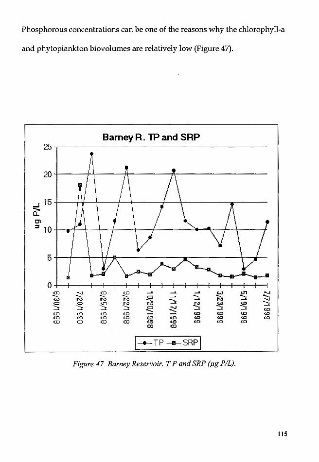
Phosphorous concentrations can be one of the reasons why the chlorophyll-a
and phytoplankton biovolumes are relatively low (Figure 47).
BarneyR. lPand SRP 25-.-~~~~~~~~~~~~~~~~~
20-+-~--+-+-~~H-~~---,p,...-~~~~~~~
...J 15 CC' Cl :;, 1 Q I •--'I l '• J ~rtl -j-1 ~Ji -.---( I I --{
5-+--+---t-~-f"-llt--~~~~---~~~~-T----
0 G) -....J co (.0 -A -A -A w (.J1 -....J - - - - 0 ....... - - - -w N N N - - -A N -A --..I 0 QJ ....,., N r'IJ ....... N -....;> ~ """'-- - ~ - CJ -....J ~ - ~
....... ....... ....... ....... - - ....... (.0 (.0 (.0 (.0 (.0 _.. ....... (.0 (.0 (.0 o'.!:) o'.!:) o'.!:) o'.!:) o'.!:) (.0 (.0 o'.!:) o'.!:) o'.!:) (.0
co co co co o'.!:) o'.!:) (D (.0 (.0
co co
1--+-TP -sRPI
Figure 47. Barney Reservoir. T P and SRP (µg PIL).
115
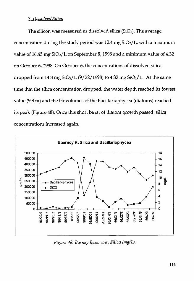
7. Dissolved Silica
The silicon was measured as dissolved silica (Si02). The average
concentration during the study period was 12.4 mg Si02/L, with a maximum
value of 16.43 mg Si02/L on September 8, 1998 and a minimum value of 4.32
on October 6, 1998. On October 6, the concentrations of dissolved silica
dropped from 14.8 mg Si02/L (9/22/1998) to 4.32 mg Si02/L. At the same
time that the silica concentration dropped, the water depth reached its lowest
value (9.8 m) and the biovolumes of the Bacillariophycea (diatoms) reached
its peak (Figure 48). Once this short burst of diatom growth passed, silica
concentrations increased again.
Baerney R. Silica and Bacillariophycea
500000 18
450000 16 400000 14 350000 12
- 300000 10 o::!
~ 250000 Cl
~ 200000 8 E
150000 6
100000 4
50000 2
0 0 ~ ~ ~ ~ ~ se ~
...... ...... ...... ...... ...... ...... ~ ~ ~ ~ ~ ~ Q Q ...... ...... ~ -(,) ...... ...... I\) ~ - - ...... I\) I\) I\) ...... ~ ~
Q ~ ~ ...... ~ ~ ~ I\) ~ ...... ...... ~ ~ ~ ...... se (i5 <O Q ~ Q (i5 <O <O
<O <O <O CX> <O <O <O <O <O <O <O <O <O CX> CX> CX> CX> CX> CX> CX> <O CX> <O <O <O <O <O <O <O
CX> CX> CX>
Figure 48. Barney Reservoir. Silica (mg/L).
116
8. Major Dissolved Cations: Na. K Mg and Ca
The concentrations of Na, Ca and Mg were between 1.5 to 6.6 mg/L
whereas the concentrations of K never rose above 0.46 mg K/L.
Ca measurements were higher during the period of diminishing water
volumes and low water levels CTune-November 1998). Inputs of water and
increases in water levels appeared to 'diluted' the Ca concentrations. At the
end of the winter 1999, Ca concentrations began to rise again (Figure 49a).
The average Ca concentration was 2.9 mg. Ca/L with a high of 4.98 mg.
Ca/Lin July 28, 1998, and a low concentration of 1.6 mg Ca/Lin February
1999.
Dissolved Na concentrations were also higher during the decreasing
water elevation and the period of constant low water levels. With increases
in water volumes and elevation, Dissolved Na concentrations increased
somewhat, but by mid-winter the concentrations of Na were at its lowest. By
the end of the winter 1999, sodium concentrations began to rise again. The
average concentration of Na was 4.4 mg Na/L with a maximum of 6.5 mg
Na/Lin October 6, 1998, and a minimum concentration of 2.4 mg Na/Lin
February 1999 (Figure 49).
117

Barmey R. Major Cations ?-.--~~~~~~~~~~~~~~~~-
611-~~~~--~~_,.__,..,.~~~~~~~-
5-H---<a----in---+-~~~~~-+-~~~~~~-
..I 4 ...... Cl E <I~ \ I i) 3 I " ".c -....... \ 'I \ I
2 I i:: ..i: --. ', ...,.. .A'""
0 rn -...J (D (.Q ---' ---' ___. w 01 - - ........... ........... a __. ........... ........... ........... WJ N N N -.... -.... __.. N __.. a CD 01 f\.) N ---' f\.) w (0 ..._ ..._ ............ ............ a --.I ............ ............ ............ ---' ---' ___. ___. -.... -.... ___. ___. ....... (£) (£) U) U) ---' ---' U) U) U) UJ UJ (.Q (.Q UJ UJ (.Q (0 (0
CD CD OJ OJ UJ UJ U) U) U)
CD CD
l__._ca --+-K __.__Mg --0- Na I
Figure 49. Barney Reservoir. Cations: Na, Ca, Mg and K (in mg/L).
-...J ---.I -.... .... UJ UJ (£)
Dissolved Mg had relatively higher concentrations during the period
of decreasing water elevation and the period of constantly low water levels
Gune-November 1998). The result of the increased water volumes was a
decrease in Mg concentrations. By the end of the winter 1999, Mg
concentrations began to rise (Figure 49). The average Mg concentrations
were 1.39 mg Mg/L, with a maximum concentration of 1.97 mg Mg/Lin
118

November 1998, and a minimum concentration of 0.64 mg Mg/Lin February
1999.
The concentrations of dissolved K were higher when water elevation
was decreasing and when the water elevation was constant although low
Gune-November 1998). The result of the increased water volumes was a
further decrease in potassium concentrations. After the winter 1999 the
concentrations of potassium began to rise (Figure 49). The average K
concentration was 0.21 mg K/L, with a maximum concentration of 0.46 mg
K/L in July 28, 1998, and a minimum concentration of 0.06 mg K/L in April
1999.
Low inflows and decreased water levels from June to November 1998
appeared to increase the concentration of cations present in Barney
Reservoir. High precipitation and inflows associated with late fall 1998 and
winter 1999 increased the volume of the reservoir and 'diluted' the
concentrations of cations. On the other hand, epilimnetic conductivity had a
similar pattern, with high conductivity during low water volumes and vice
versa. The major anions (Chloride and Sulfate) were not measured
consistently during this study, and only one sample from Barney Reservoir is
reported here (Figure 24b). The dissolved chloride concentration
measurement was higher than the chloride measurements for Hagg Lake,
119
and the dissolved sulfate concentrations were lower than the Hagg Lake
measurements.
9. Trophic State Indices
TSI for Barney Reservoir was calculated using the formulae proposed
by Carlson (1977). Figure 50 portrays these variations for TSI for Secchi
depth, Chlorophyll-a and Total Phosphorous.
The calculated TSI for Secchi depth had an average of 44.27 units, with
the highest values occurring October 20, 1998 at 51.9, during the period of
mixed water column (Late September, 1998 to April 1999). Decreases
occurred before and after the mixing period. The effects of increased water
volumes and elevations on the TSI for Secchi depth were minimal. This
occurred probably because there was little human activity in the watershed
and most of the suspended materials came from the shores of the reservoir
and the newly inundated areas.
The calculated TSI for chlorophyll-a had an average of 37.06, with the
highest value calculated for September 8, 1998 at 45.4 units, and the lowest
on December 1999 at 25.7 units. The pattern of the TSI for Chlorophyll-a was
identical to the actual chlorophyll-a measurements.
The calculated TSI for total phosphorus had an average of 36.8 units.
Low TSI-TP occurred on September 22, 1998 and May 1999 (19.7 and 19.05
units respectively), outside of the period of mixing. Also, there was some
120
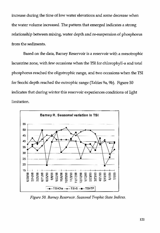
increase during the time of low water elevations and some decrease when
the water volume increased. The pattern that emerged indicates a strong
relationship between mixing, water depth and re-suspension of phosphorus
from the sediments.
Based on the data, Barney Reservoir is a reservoir with a mesotrophic
lacustrine zone, with few occasions when the TSI for chlorophyll-a and total
phosphorus reached the oligotrophic range, and two occasions when the TSI
for Secchi depth reached the eutrophic range (Tables 9a, 9b). Figure 50
indicates that during winter this reservoir experiences conditions of light
limitation.
Barney R. Seasonal variation in TSI
55~----
50+---~~---
::&Jfl\"~ ~ - -
25 +----lc-t---~------t---7-
20 ~--------;lit---
15 (X) (X) (X) (X) (X) (X) (X) (X) (X) (X) (X) (X) en en en en en en en en en en en en en en en en en en en en en en ~ en en en -.... -.... -.... -.... -.... -.... -.... -.... -.... -.... -.... -.... -.... -.... -.... -.... -.... -.... C> v (X) ~ U') (X) C\J UJ C> C"') I"- C> C\J C"') C"')
~ en I"- I"-
C"') :i::::::. C\J :i::::::. C\J -.... C\J -....
~ -....
:i::::::. :i::::::. :i::::::. C\J C\J ~ -.... -.... -.... -.... -.... en en- C> ~ -.... -.... -.... UJ I"-UJ I"- I"- (X) (X) ~ C> ~ ~ C\J ~ C\J C"') v U')
~
[--+--TSl-Cha -+-TSl-S ----- TSl-TP [
Figure 50. Barney Reservoir. Seasonal Trophic State Indices.
121

10. Nutrient Ratios
The average value of Barney Reservoir epilimnetic total nitrogen -
total phosphorous (TN:TP) mass ratios was 14.67, with a high ratio of 60.5
calculated for November 17, 1998, and a low ratio of 2.2 calculated for July
1999. The three high TN:TP ratios occurred when either total nitrogen
increased (Nov. 1998) or total phosphorus decreased. Only in five of the
eighteen calculated TN:TP ratios the values were lower than 7, indicating
that some nitrogen limitation occurred (Figure 51). However, total
phosphorus was generally low when compared to total nitrogen, the
biological activity of the phytoplankton was also low (chlorophyll-a),
therefore the information contained in the TN:TP is more difficult to assess
without first analyzing the individual nutrient concentration measurements.
The effects on the nutrient concentrations of increased flows and water
volumes were minimal, particularly if compared with the effects of increased
flows on nutrient concentrations in Hagg Lake
The average dissolved silica - total phosphorus (Si:TP) mass ratio was
1486.2 units. The highest Si:TP ratios were calculated at 5267.2 in September
22, 1998, and at 4007 in May 1999. These two highs occurred outside the
period of the mixed water column. The average Si:TP during the period of
mixing was 1063.7 or 485 units lower than the average for the study period,
and 4203.5 units lower than the maximum Si:TP ratios. High water inflows
122
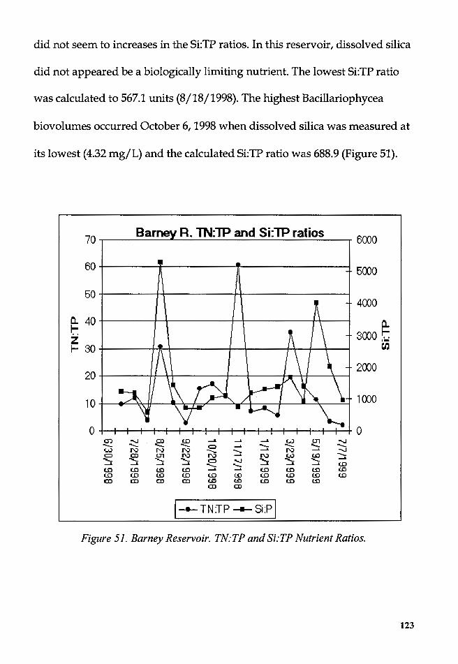
did not seem to increases in the Si:TP ratios. In this reservoir, dissolved silica
did not appeared be a biologically limiting nutrient. The lowest Si:TP ratio
was calculated to 567.1 units (8/18/1998). The highest Bacillariophycea
biovolumes occurred October 6, 1998 when dissolved silica was measured at
its lowest (4.32 mg/L) and the calculated Si:TP ratio was 688.9 (Figure 51).
70 , Barney R. lN:TP and Si:TP ratios , 6000
60+-~~-,1-~~~~~~~~~~~-1 5000
50-+-~~-+--i--~~~-++~~~~~~-l
4000
o.. 40-!-~~+-+~~~-r-t--~-:-~rx---i ~
~ so-L-~~HH~~~-t-T-~-r\1-"\~ 0..
3000 t ·-~ 2000
20-+-~~------~~~-+--+-~--+~..+----'l--t
10 I .,c \\ II • \= I ,r '-w/ 1 J • '\ • I 1000
0 I I I I I I I I I I I I I I I I I I 1-1 0 en --..I CD (0 __.. ....... __.. w (J'j --..I
--- --- - --- 0 ..... --- --- - ---w N N N - - ...... N ..... ........ C) (D (J'j I\) J\) ..... I\) w U)
......_ ...._ ...._ .._ ....._ C) "-.I
...._ ...._ .._ ...... __.. __.. ....... __..
--- - __.. __. ....... (0 (£) (£) c.:o (£) ...... ..... (£) (£) c.:o .:.0 (£) (£) U) (0 (0 U) (0 (0 U) (£) (D (D CD (D .:.0 t.:. (£) (£) c.:o
(D CD
I---TN :TP ------ Si:P I Figure 51. Barney Reservoir. TN:TP and Si:TP Nutrient Ratios.
123

c) Biological factors
1. Phytoplankton:
During this period of this study 11 species dominated the measured
total biovolumes (96.1 % ). However, limited phosphorus availability and
unstable physical conditions in the lacustrine zone of Barney Reservoir could
have interfered with the development of a biologically active phytoplankton
community, as measured by the concentrations of chlorophyll-a. Whenever
peaks in the chlorophyll-a measurements occurred, the biovolumes of
Dinobryon sertularia and Cryptomonas sp. were the most dominant. Of the 11
species, five were colonial species and six were not (Figure 52).
Chrysophytes (Dinobryon sp.) dominated the total biovolumes, followed by
cryptophytes (Cryptomonas sp.), chlorphyceas (Oocystis borgei, Chlamydomonas
sp.) and bacillariophyceas. Euglenophytas and Cyanophytes were also
represented in low biovolumes during the period of low water elevation.
Dinoflagelates were present throughout the sampling period as well (Table
6).
124
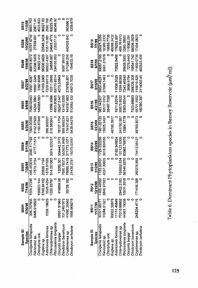
.....
N
UI
Sam
ple
ID
seec
ies
Cru
cige
nia
tetr
aped
ia
Nav
icu/
oid
sp.
Ch/
orph
yta
unk.
E
ugle
na s
p.
Ast
eri
on
ela
form
osa
Ch
/am
ydo
mo
na
s sp
. R
hizo
sole
nia
long
iset
a O
ocy
stis
bo
rge
i D
ino
bry
on
ba
vari
cum
C
ryp
tom
on
as
sp.
Din
ob
ryo
n s
ertu
/aria
Sam
ple
ID
Se_e
cies
C
ruci
geni
a te
trap
edia
N
avi
culo
id s
p.
Chl
orph
yta
unk.
E
ugle
na s
p.
Ast
eri
on
ela
form
osa
Ch
/am
ydo
mo
na
s sp
. R
hizo
sole
nia
/ong
iset
a O
ocy
stis
bo
rge
i D
inob
ryon
ba
vari
cum
C
ryp
tom
on
as
sp.
Din
obry
on s
ertu
lari
a
8S01
8S
02
8S03
8S
04
8S
05
8S
06
8S
07
8S
08
8S
09
8S
10
6/30
/98
7/14
/98
7/28
/98
8/11
/98
8/25
/98
9/8/
98
9/22
/98
10/6
/98
10/2
0/98
11
/3/9
8 30
6.70
7905
15
54.2
1249
44
6.45
3019
36
40.1
1719
2 15
04.0
0395
75
99.0
2483
19
561.
6287
46
878.
8072
16
797.
6716
90
93.7
53
6406
.916
522
0 17
579.
3154
47
77.7
1571
91
42.8
7929
14
248.
3561
18
887.
3345
32
336.
5305
27
559.
037
2387
1.41
0
1568
23.1
44
0 0
1190
.879
48
1469
85.5
93
3382
.658
8 66
922.
411
0 40
23.8
03
0 37
46.9
4152
23
558.
7194
0
0 0
4745
9.33
69
9630
0.96
29
2954
6.34
39
9032
7.53
13
59.1
9629
55
26.4
294
1678
.915
26
0 39
6.90
5507
0
7328
.091
19
9093
3.43
67
1351
10.8
81
2682
.168
0
1039
.837
87
914.
0010
83
3974
.523
237
518.
5806
41
1355
6.90
66
1031
1.09
35
2465
8.66
7 24
645.
4776
83
229.
79
0 0
0 0
0 49
53.8
0805
69
770.
8514
33
4155
.882
22
0377
.01
6834
8.92
68
951.
9196
3 41
9899
.98
1308
2.30
1 30
4442
.317
2 78
107.
1704
29
247.
5147
40
75.5
3849
0
0 0
131.
2467
973
0 76
90.7
8373
553
621.
9465
58
9.66
9234
13
140.
9355
0
5097
.991
13
0 0
4109
2.20
502
2972
8.18
2 78
886.
7 41
9 27
1773
.137
1 17
4147
.621
14
3187
.663
27
9785
.801
37
1289
.256
44
2426
.843
26
3590
.3
1595
.968
219
0 21
436.
3751
15
079.
0315
7 64
38.9
4219
51
2652
.122
64
013.
7035
15
4633
.16
0 12
08.6
79
8S11
8S
12
8S13
8
S1
4
8S
15
8S
16
8S
17
8S
18
8S
19
11
/17/
98
12/1
0/98
1/
1219
9 2/
23/9
9 3/
23/9
9 4/
21/9
9 5/
19/9
9 6/
7/99
71
7/99
10
321.
9527
1 14
65.4
9562
11
53.5
0107
17
25.0
2025
5 19
81.6
3135
98
3.14
2927
59
52.4
8251
39
067.
2165
28
021.
3256
11
084.
5132
7 38
46.9
7583
40
37.3
0605
30
18.8
2455
6 15
605.
5491
16
517.
0152
27
084.
1463
30
61.2
7678
18
389.
2332
0
0 0
0 0
3549
7.70
99
0 0
1505
5.77
38
6932
2.32
678
0 0
0 48
798.
3977
0
0 0
4928
8.24
32
1117
4.40
849
0 0
2162
.349
834
0 19
71.8
2514
11
938.
5029
73
822.
8486
17
6253
.897
70
310.
6660
2 29
402.
3163
15
9952
.634
10
7123
.630
6 24
1790
.967
55
873.
6532
12
99.8
6365
0
409.
7619
13
4496
1.19
338
1003
1.25
18
5614
6.93
79
8396
5.76
975
1356
4.17
78
5383
.655
44
7243
.462
42
2660
8.29
32
2283
.389
51
0 0
0 0
0 0
9590
.579
4 72
78.4
443
1163
62.0
91
0 0
0 0
0 73
23.6
8663
28
8220
.308
15
8541
.742
68
026.
2629
24
5204
.471
6 17
1416
.368
26
0276
.859
74
412.
5512
7 88
769.
8073
58
721.
5902
11
8510
.825
11
609.
0735
17
434.
0623
0
0 0
0 0
1803
80.3
97
2114
303.
45
4005
23.4
06
0
Tab
le 6
. Dom
inan
t Phy
topl
ankt
on s
peci
es in
Bar
ney
Res
ervo
ir (
µm1
ml)
.
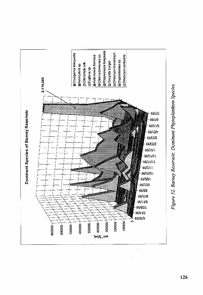
.....
N a--
-·"'~
r-,_
,._
_
••-·-
· -·-···-••
••••
-
""'
•
9000
00
8000
00
7000
00
6000
00
5000
00
...J .€.
4000
00
M
c E
3000
00
:I
2000
00
1000
00
Do
min
ant
Sp
ecie
s o
f B
arn
ey R
eser
voir
····
····
-·-·
Iii
Cru
cige
nia
tetr
ap
ed
ia
l!ll N
avi
culo
id s
p.
D C
hlor
phyt
a un
k.
o E
ugle
na s
p.
ll!IA
ster
ione
la f
orm
osa
mC
hla
myd
om
on
as
sp.
lml R
hizo
sole
nia
long
iset
a
EJO
ocys
tis b
org
ei
I E:J D
ino
bry
on
ba
vari
cum
1I1C
rypt
omon
as s
p.
o D
ino
bry
on
ser
tula
ria
...... ~
::: ~ ~
en
en
en
~
;:::-
l.l:?.
LC>"
to" ~
Fig
ure
52.
Bar
ney
Res
ervo
ir.
Dom
inan
t Phy
topl
ankt
on S
peci
es .
~~--~---
·---
--
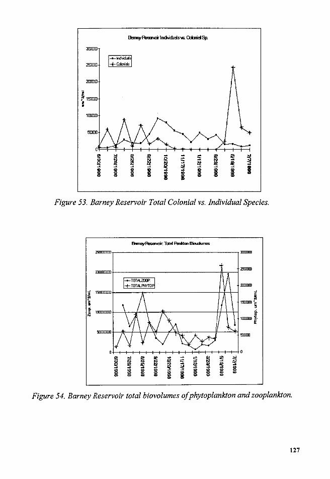
JJllllJ
2DllD
:milD
~ 19lDll ! •
lCIIIlD
!DlDl
0
~ I
Ebn~Feserwi"lnd\idJds\S. Qbilll Sp.
~ ~
~
~ I
~ I
~ I
-.Q
~ ... I
--::i: ~ ... 4D
i
--... ~ I
~ I
~ ! I
~ :I
I
Figure 53. Barney Reservoir Total Colonial vs. Individual Species.
flmnl¥F'lesm0r. Tcid Pmldcro 80\durnes
2DJIDlll Dlllll
.+
2ID1UID I ~ imon I\ A 1--rnrrn I :mxm { ~I
~ 7\ K m\l,-t g 100lIDlll \ 1- I N I I 1 8-
lCDJlD f ml ~ v l ~. L~ ~. v ±>ti
!ilDlJ
O I I I I I I I I I I I I I I I I I I I I 0
.e ~ .e le Q - - ~ .ll! ~ .., "' "' "' - "' ~ .Q ~ ~ ~ "' - ~ 3 ~
i8 s ~ l8 l8 l8 l8 l8 l8 l8 l8 l8 U> (I) (I) (I) (I) U> U> U>
(I) (I)
Figure 54. Barney Reservoir total biovolumes of phytoplankton and zooplankton.
127

2. Zooplankton
The total biovolumes of the zooplankton populations in Barney
Reservoir was dominated by four species. The most dominant was a species
of cyclopoid, Diacyclops thomasi, a raptorial, which exerted predation
pressure on the herbivorous zooplankton. The other dominant species were
two species of Eucladocerans: Bosmina longirostris, a bosminid, Daphnia
catawba, a daphnid, and Asplanchna priodonta, a rotifer. However, protozoans
and many other species of rotifers and eucladocerans were also present in
this reservoir. During this study, no live calanoids (a herbivorous
zooplankton present in Hagg Lake) were encountered, only residual
exoskeletons were seen.
The zooplankton species encountered in Barney Reservoir were
grouped according to their feeding habits as raptorials, filter feeders, grazers
and omnivores (including in the omnivores the nauplii of the copepods). The
dominant groups of zooplankton according to their feeding habits were the
raptorials (cyclopoids) and grazers (eucladocerans). Their dominance
diminished during the period of mixing and omnivores (rotifers) increased
their biovolumes. From December 1998 to March 1999 high water volumes,
high outflows, and low phytoplankton biovolumes might have helped to
decrease the biovolumes of all the zooplankton species.
128

.... N
\C
Sa
mp
le ID
B
S02
B
S03
B
S04
B
S05
B
S06
B
S07
B
SO
S
BS
09
BS
10
S~ecles
7/14
/98
7/28
/98
8/11
/98
8/25
/98
9/8/
98
9/22
198
10/6
/98
10/2
0/98
11
/3/9
8 B
osm
ina
long
irost
ris
2674
349.
568
0 0
4871
662.
952
0 61
8857
7.51
33
1530
9.38
0
2952
5308
.2
Asp
lanc
hna
prio
dont
a 0
0 0
0 13
3938
49.9
0
0 17
6484
969
2180
3304
5 D
aphn
ia c
ataw
ba
8023
0487
.03
1053
3642
1 13
6470
190
1993
9576
6.5
5783
7079
.1
7097
7759
.9
2712
5258
.6
2440
4360
.7
3097
0603
C
yclo
poid
s (c
opep
odid
s 1-
V)
7658
3646
.71
2433
5877
8 18
5193
182
4094
3066
2.2
8097
1910
.8
6210
8470
.1
3164
6135
78
1307
91.1
69
3741
50.6
D
iacy
clop
s th
omas
i 10
1139
0382
28
0856
937
6188
5775
1 85
0728
480.
1 56
8223
935
1892
7402
7 12
0556
705
2046
3384
4 33
0353
098
Sa
mp
le ID
B
S11
B
S12
B
S13
B
S14
B
S15
B
S16
B
S17
B
S18
B
S19
S~ecies
11/1
7/98
12
110/
98
1/12
/99
2123
/99
3/23
/99
4/21
/99
5/19
/99
617/
99
7171
99
Bos
min
a lo
ngiro
stris
17
0113
7.64
8 13
0071
0.07
0
2376
297.
241
2529
844.
09
8538
857.
7 76
1791
44.5
48
2556
48.9
10
4868
73.6
A
sp/a
nchn
a pr
iodo
nta
5613
7542
.39
2341
2781
.2
0 0
0 0
2856
7179
.2
3537
0277
1 15
7303
10.4
D
aphn
ia c
ataw
ba
1391
8398
.94
2660
5433
.2
1331
0284
.2
2657
1323
.7
9199
433.
04
4657
5587
.4
2597
0162
9 33
7789
542
7865
1552
.2
Cyc
/opo
ids
(cop
epod
ids
1-V)
19
4857
58.5
2 12
4158
68.8
62
1146
5.96
46
2729
88.1
32
1980
15.7
20
3768
19.5
10
9074
684
1903
9046
9 90
0917
78
Dia
cycl
ops
thom
asi
1113
4719
1.5
8986
7241
.1
3943
7879
.1
1036
9297
0.5
1042
6024
1 17
0777
154
6232
8390
9 98
2660
487
4576
0903
1
Tab
le 7
. Dom
inan
t Zoo
plan
kton
spe
cies
in
Bar
ney
Res
ervo
ir (
µm
j ml)
.

on
I\.) .j>. 0
m
8 8 0 umAJfml 0
0
g 0
0
0 0 C5
0 0
0 0
0 0
g g 0 0
0 0
0 ......
0 I\.)
~ 0
§ 0
0 g
m DI
~ '<
iii Ill CD
~ 0 ::;· c 0 3 :;· DI ::i -N 0 0 'C iii ::i
~ ::i Ill 'C CD n ;· Ill

14CXXJOOOOO
1200000000
1000000000
-~----Barney Zooplankton by Feeding gropus
•Eggs
•Protozoans
E!Rotifers
o Eucladocerans
11 Cyclopods
~ ~
g;_ g;_ ~ ~ ~
. L - ~ - N
Figure 56a. Barney Reservoir zooplankton, by feeding groups (biovolumes).
When the large herbivores zooplankton and the small zooplankton
species are considered apart from the large, raptorial cyclopoids, there is a
clear dominance of the large bodied daphnids during the periods of
stratification Gune-early September 1998 and Spring 1999) and their decline
occurs at the same time water levels drop and the period of mixed water
column begins. From December 1998 to March 1999 a slight dominance of
daphnids and Synchaeta sp. (Figure 56a and 56b).
131
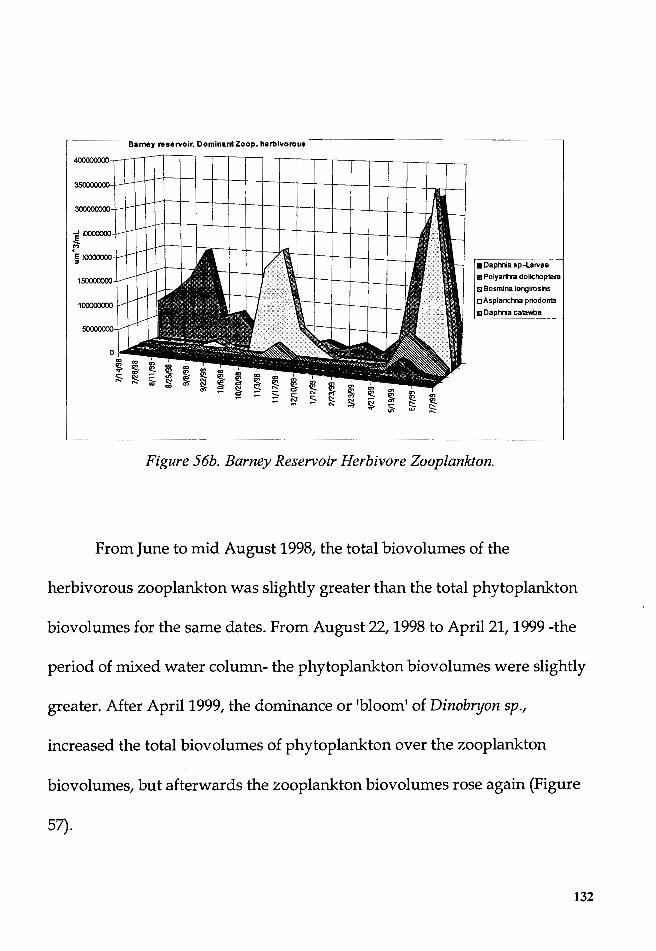
400000000
350000000
300000000
...J 0000000
~ . E XlOOOOOO " 150000000
Bamey reservoir. Dominant Zoop. herbivorous
~ ~
• Daphnia sp.-Larvae
11 Polyarthra dolichoptera
Ill Bosmina longiros1ris
oAsplanchna priodonta
111 Daphnia catawba
Figure 56b. Barney Reservoir Herbivore Zooplankton.
From June to mid August 1998, the total biovolumes of the
herbivorous zooplankton was slightly greater than the total phytoplankton
biovolumes for the same dates. From August 22, 1998 to April 21, 1999-the
period of mixed water column- the phytoplankton biovolumes were slightly
greater. After April 1999, the dominance or 1bloom1 of Dinobryon sp.,
increased the total biovolumes of phytoplankton over the zooplankton
biovolumes, but afterwards the zooplankton biovolumes rose again (Figure
57).
132
The prolonged mixing of the water column seemed to be an important
factor controlling the plankton dynamics of Barney Reservoir, with more
photosynthetic activity by the phytoplankton and greater zooplankton
biovolumes occurring during the periods of stratification. While the water
levels decreased or were low (September to November 1998), the effects of
mixing on the phytoplankton were positive because nutrients from lower
depths reached the photic zone favoring the growth of Cryptomonas sp.,
Rhizosolenia sp., Asterionela sp., and euglenoids among other species. As
individual species dominated this short period of low water levels and
mixing, small-bodied zooplankton, having less predatory and competitive
pressure from larger zooplankton, were able to increase their biovolumes.
The onset of high precipitation and water volumes, low light and
lower temperatures was followed by a decrease in the phytoplankton and
zooplankton biovolumes. The return of stratification and more stable
conditions, at the end of April 1999, favored increases in the biovolumes of
cyclopoids, eucladocerans and fast swimming rotifers.
133

Barney R: Total Biov. of Phytop. and Herb. Zoop.
Ph:ytop. (um"31ml) Herb. Z'oop. (um"31ml)
3XlODJ "BJOODJO --o- Total Phytop.
2&JOJX) I , --Herb. Z.Oop. 1 rj"' 'A I 4lJOOllJO
3&10:0000
2000JX)+-~~~~~~~~~~~~~~~~~~~~~~-+--+-+-~-+ 3X)oo:JOOO
2&lOOllJO 1&JODJ-l--~~~----:-~~~~~~~~~~~~~~~t--t---\~
20000llJO
100COD I Jr }\\ / >n 11
11 1
1 I 1&JOODJO
10000llJO rococo
&JOOOll)
0 0 !n-..J-..JCDCD (.0 (.0
8~~:!§;! ~ ~ ~ ~ s s; ~ ~ ::::i: ::::i: ::::i: ::::i: ::::i: to::::i:::::i:a::::i:-...ia::::i:
!:8 !:8 !:8 !:8 !:8 ffi !:8 !:8 ffi !:8 ffi ffi !:8 CD CD CD CD CD CD CD (.0 CD (.0 (.0 UJ
"-.) w ~ ui
8 8 !S! ffi ::::i: ::::i: ::::i: ::::i:
!:8 !:8 !:8 !:8 (.0 (.0 (.0 (.0
en ~ (.0
!:8 CD CD CD
Figure 57. Barney R. Total biovolumes of phytoplankton and herbivore zoop.
3. Fish predation
Cutthroat trout (Oncorhynchus clarki clarki) were observed in the
reservoir. During the study period, however, the reservoir was not being
stocked with fish, nor was it open to recreational fishing.
134
4. Species richness
In this study, the Shannon-Weiner index of diversity was used to
measure the information content of the sample. The calculated values of this
index, for zooplankton and phytoplankton in Barney Reservoir, are given in
figure 58a. The average diversity measured was 1.62 bits per individual for
the zooplankton and 2.04 for the phytoplankton (formula 1.0, Species
diversity heading of Hagg Lake section).
The graph shows that the index for both the zooplankton and
phytoplankton increases as the summer and fall 1998 progresses, and only
decreases for the phytoplankton in December 1998 (1.009 bits). This decrease
in the phytoplankton index could be related to increases in water volumes.
The winter 1999 conditions did not seem to have a great impact on either the
zooplankton and phytoplankton. During the spring of 1998, (May 1999) the
phytoplankton index decreased when the Dinobryon sp. was dominant. In all
of the cases when the phytoplankton index was low, dominance in the
proportions to the total biovolumes was exerted by one of the species
present.
The trends for the zooplankton Shannon-Weiner index is less variable
since the species composition did not change much during the period of this
135
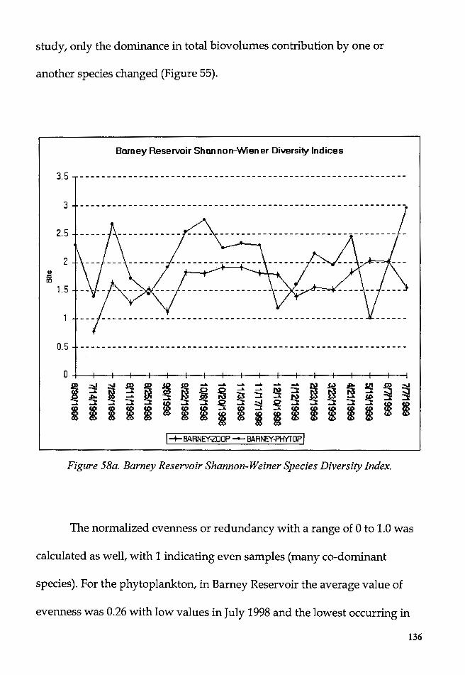
study, only the dominance in total biovolumes contribution by one or
another species changed (Figure 55).
Q .c: m
Barney Reservoir Shonnon-'Wiener Diversity Indices
3.5 --------------------------------------------------------------
3 ·-------------------------------------------------------------
2.5
2
1.5
0.5 ·-------------------------------------------------------------
0+--+---l~-+--+----11---t--+-~----+--+~t---+---+~+--+---+~-+--i
! ~ ~ ~ ~ ~ ~ i ~ ~ s i i i i i I i i i i j
.... 5;1~~~ .... Q? ..... llJ. ...... ~ I m m m i m m m I-+- 8.6.RNEY·ZDOP --8.6.RNEY·PHYTOP I
Figure 58a. Barney Reservoir Shannon-Weiner Species Diversity Index.
The normalized evenness or redundancy with a range of 0 to 1.0 was
calculated as well, with 1 indicating even samples (many co-dominant
species). For the phytoplankton, in Barney Reservoir the average value of
evenness was 0.26 with low values in July 1998 and the lowest occurring in
136
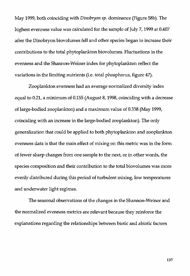
May 1999, both coinciding with Dinobryon sp. dominance (Figure 58b). The
highest evenness value was calculated for the sample of July 7, 1999 at 0.407
after the Dinobryon biovolumes fell and other species began to increase their
contributions to the total phytoplankton biovolumes. Fluctuations in the
evenness and the Shannon-Weiner index for phytoplankton reflect the
variations in the limiting nutrients (i.e. total phosphorus, figure 47).
Zooplankton evenness had an average normalized diversity index
equal to 0.21, a minimum of 0.155 (August 8, 1998, coinciding with a decrease
of large-bodied zooplankton) and a maximum value of 0.338(May1999,
coinciding with an increase in the large-bodied zooplankton). The only
generalization that could be applied to both phytoplankton and zooplankton
evenness data is that the main effect of mixing on this metric was in the form
of fewer sharp changes from one sample to the next, or in other words, the
species composition and their contribution to the total biovolumes was more
evenly distributed during this period of turbulent mixing, low temperatures
and underwater light regimes.
The seasonal observations of the changes in the Shannon-Weiner and
the normalized evenness metrics are relevant because they reinforce the
explanations regarding the relationships between biotic and abiotic factors
137
Barney Reservoir Diversity Even esss (1-0)
0.45
0.4
0.35
0.3
0.25
0.2
0.15
0.1
0.05
0-t---+---i~-+--+-~l---+---+~+---+--t-~-t--t---+~-t---+---i~-+----1
~ ~ ~ ~ ~ ~ ~ - - - - - - ~ ~ ~ ~ ~ ~ ~ ~ ~ ~ ~ ~ ~ ~ § ~ ~ ~ ~ ~ ~ ~ ~ ~ ~ i i i i i ~ i i i i i i i i i i i I I
I+ 8/l.RNEY-ZDOP _.._ 8/l.RNEY-PHYTOP I
Figure 58b. Barney Reservoir Normalized (Diversity) Evenness.
138
SUMMARY
Understanding the dynamics and characteristics of reservoirs is a
complex and difficult task, but nonetheless achievable if a methodical
approach, coupled with some awareness of the interacting factors at work,
can be used to partition or select one particular dimension or problem of
interest. Once this dimension is selected, the other elements left out can still
be referenced to aid in explaining the changes observed.
A conceptual model was developed to identify the many dimensions
and factors that define a theoretical reservoir. The chosen dimension of
interest for this study, based on the theoretical model, was the dynamics of
the planktonic successions from the June 1998 to early July 1999.
The PEG model for lakes was adapted to describe the plankton
dynamics of Hagg Lake and Barney Reservoir. To do this the climatic regime
and the geographic location were taken into consideration.
The northwest corner of the state of Oregon had a rainy, storm driven
season; it began in November 1998 and lasted until April 1998 (Figure 6).
The passage of these weather fronts and their accompanying winds caused
constant mixing of the water columns, and changes in water levels of Hagg
139
Lake and Barney Reservoir. These constant disturbances could be
interpreted, from the point of view of the plankton, as a fall overturn that
persists until the end of winter, when the operators of the dams allows the
water levels to stabilize.
It is at this point that the PEG model begins to describe the succession
of the plankton. Human influences, in terms of watershed land use practices,
were also taken in consideration.
In Hagg Lake, the impact of human activities on the watershed could
have caused more sediments and nutrients to enter the reservoir. For
example the percentage of land used in human activities is only 3.5% and yet
the overall water quality of the reservoir at the lacustrine zone is lesser than
the water quality of Barney Reservoir, where no permanent human
settlements existed in its watershed boundaries during the study period.
Another human activity that deserves to be considered is the annual stocking
of the reservoir with warm water fish, and the impact that this has on the
predatory zooplankton - herbivorous zooplankton and the phytoplankton
relationships.
140

Hagg Lake
The geographical elements such as vegetation cover of the watershed,
the orientation and closeness of the surrounding hills, the geometry of the
reservoirs and the general orientation of the main axis in relation to the
predominant weather patterns were important for both Hagg Lake and
Barney Reservoir.
In Hagg Lake, the differences between the maximum and minimum
water elevations and the water volumes were important to the yearly
hypolimnetic dissolved oxygen concentrations. The hydraulic mean
residence times were long enough as to be considered irrelevant in terms of
the planktonic losses by washout (Reynolds, 1984). Human influences such
as clear-cutting of the forests and housing developments need to be taken in
consideration.
The distribution of the temperature in the water column appeared
influenced by the water elevation. However the high water storage capacity
of Hagg Lake could have made this influence less important by its effect on
the residence times and high volumes of inflows.
141
The photic zone and Secchi depth were affected by the amount of
suspended materials carried into the reservoir by the main tributaries. This
was evident in the observed turbidity measurements. The summer
disturbances that occurred in the watershed, which increased sediment
loadings to the reservoir, had a more noticeable impact on the turbidity than
the larger inputs occurring during the winter.
During winter conditions, a dilution effect caused by the high inflows,
the mixing of the water column and rapid settling of the particles keeps the
turbidity low. During summer, inflows are less and the thermal stratification
prevents mixing of the water column, as sediments enter the reservoir they
will be concentrated in the underflows or overflows within the stratified
water column.
The pH in Hagg Lake during the period of stratification seemed
influenced by the photosynthetic activity of the algae in the photic zone
(summer 1998). Increases in winter inflows and mixing of the water column
kept the pH between 6.7 and 6.9. The close relationship between
conductivity, redox, and pH was also evident in the time-depth diagrams.
Low redox and dissolved oxygen values in the hypolimnion explained the
observed increases in reduced nitrogen. Alkalinity, cations and dissolved
inorganic carbon concentrations followed similar trends with decreases
during high water inflows and high water storage. However, dissolved
142
potassium was found in the low concentrations, when compared to the other
cations.
Hagg Lake chlorophyll-a concentrations were a good reflection of the
levels of phytoplankton activity. Summer peak values occurred at the same
time that biovolumes peaks of Synedra radians, Fragilaria crotonensis and
Cryptomonas sp. were noted. Winter lows of chlorophyll-a were in agreement
with low phytoplankton biovolumes, low temperatures and low irradiance.
Nitrogen concentrations in the epilimnion during the study period were low
when precipitation and inflows were low, and increased as the rainy season
progressed. Ammonium nitrogen was low, with some hypolimnetic
increases during the period of summer anoxia. Epilimnetic total phosphorus
concentrations were correlated with the water levels and the chlorophyll-a
measurements whereas SRP concentrations were generally low ( 4.26 µg
P/L).
Silicon measured as dissolve silica (Si02) was found in relatively high
concentrations, and the biovolumes of the diatoms (Bacillariophycea)
indicated that silicon was not a limiting nutrient for these algae.
The average of the trophic state indices (TSI) indicated that Hagg Lake
could be identified as having a mesotrophic lacustrine zone. The total
nitrogen- total phosphorus (TN:TP) mass ratios showed that for 37% of the
time Hagg Lake was under nitrogen limitation conditions, with high TN:TP
143

peaks that coincided with enhanced biological activity or with high inflows
during the rainy season (November 1998 to March 1999).
Barney Reservoir
The influence of the geographical elements was more evident in the
case of Barney Reservoir. Generally, the winds came from the West (Pacific
Ocean), and since the main axis of Barney Reservoir is oriented in an east to
west direction, these winds generated waves and influenced most of the
reservoir surface and its shores.
The differences between the maximum and minimum water
elevations and water volumes in Barney Reservoir were extreme (Table 1).
The impact of these extreme changes was noticeable on the water column
mixing dynamics. As a result the changes in water volume and period of
mixing played an important role in determining the succession of both the
phytoplankton and the zooplankton.
The hydraulic mean residence time was moderate and could not be
linked to planktonic losses by washout. Another important element
controlling the planktonic dynamics of this reservoir during this study
period was the low impact of human activities reflected in the percentage of
vegetation cover of the watershed (93.6 % ). High vegetation cover and low
144
human influences had as consequence a surface runoff with low nitrogen,
phosphorus and sediment loadings from runoff. This in turn caused the
waters of Barney Reservoir to have low concentration of nutrients, higher
average photic depth and relatively low chlorophyll-a concentrations,
particularly when compared with Hagg Lake.
The distribution of the temperature in the water column was
definitely influenced by the changes in water elevation and water storage.
These changes forced the hypolimnetic waters to warm up considerably and
the dissolved oxygen concentration to diminish. Also, as water levels
dropped, the kinetic energy necessary for the wind to mix the water column
was less, and thus mixing began in the middle of September 1998. With
increases in the water elevation and water volumes, the photic zone and
Secchi depth were affected but not in the same degree that Hagg Lake was.
Turbidity was more influenced by falling water levels than by increased
water levels, likely due to sediments being disturbed as the waters receded
from the small coves of the reservoir.
The epilimnetic pH of Barney increased during the period of
stratification and high biological activity, and decreased in the hypolimnion.
Epilimnetic redox was low during the summer and appeared influenced by
the biological activity. Hypolimnetic redox was slightly higher that
145

epilimnetic redox and reinforced the hypothesis that hypolimnetic anoxia in
Barney Reservoir was temperature controlled.
The pattern of the epilimnetic conductivity was similar to the pattern
for the cations and alkalinity concentrations, with higher values during the
period of low and decreasing water levels (concentration effect), and lower
concentrations when inflows and water volumes began rise (dilution effect).
However, dissolved potassium was found in the low concentrations, when
compared to the other cations.
The epilimnetic chlorophyll-a in Barney Reservoir was relatively low,
with higher activity during the period of low water elevation and higher
temperatures. Low light conditions and lower temperatures could have
contributed to low chlorophyll-a measurements during the winter of 1999.
As in the case of Hagg Lake high chlorophyll-a values were linked to high
phytoplankton biovolumes (Cryptomonads sp. and Dinobryon sp.).
Total nitrogen concentrations were generally less than 200 µg N/L
and the only increase occurred at the start of the rainy season. The likely
explanation was that nitrogen trapped in the sediments might have been re
suspended by the onset of the rainy season and increases in water volumes.
Nitrate+nitrite nitrogen had a similar occurrence. Ammonium nitrogen was
generally low, with concentrations near the detection limits. The dynamics of
phosphorus was difficult to appraise because of the low total phosphorus
146
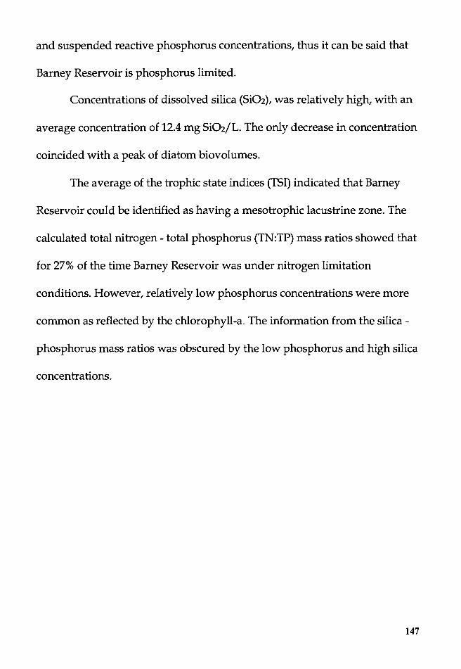
and suspended reactive phosphorus concentrations, thus it can be said that
Barney Reservoir is phosphorus limited.
Concentrations of dissolved silica (Si02), was relatively high, with an
average concentration of 12.4 mg Si02/L. The only decrease in concentration
coincided with a peak of diatom biovolumes.
The average of the trophic state indices (TSI) indicated that Barney
Reservoir could be identified as having a mesotrophic lacustrine zone. The
calculated total nitrogen- total phosphorus (TN:TP) mass ratios showed that
for 27% of the time Barney Reservoir was under nitrogen limitation
conditions. However, relatively low phosphorus concentrations were more
common as reflected by the chlorophyll-a. The information from the silica -
phosphorus mass ratios was obscured by the low phosphorus and high silica
concentrations.
147

.... "'" QC
I Pla
nk
ton
Eco
logy
Gro
up
Mo
del
I 1.
End
of W
inte
r. M
ore
light
an
d N
utrie
nts.
Unl
imite
d ~ 2
.Zoo
plan
kton
population~ 3
. F
ast g
row
ing
herb
ivor
es ~ 4
. Hig
h co
mm
unity
filtr
atio
n ra
te H
5. 'C
lear
wat
er'
phas
e.
grow
th s
mal
l; ce
ntric
dia
tom
s an
d ar
azin
a in
crea
ses.
fo
llow
ed b
y sl
ow g
row
ing
by
zoo
p.
Dec
reas
es in
N
utrie
nt r
ecyc
ling
by
graz
ing
and/
or C
rypt
ophy
cea
zoop
lank
ton
phyt
opla
nkto
n po
pula
tions
I
.L 6.
D
ecr
ea
ses
in h
erbi
voro
us
7.
Fis
h pr
edat
ion
acce
lera
tes
decl
ine
8. P
hyto
plan
kton
sum
mer
cro
p bu
ilds
9. C
rypt
ophy
ceae
and
~ 1
0. A
lgal
gro
wth
nut
rient
-zo
opla
nkto
n.
of h
erbi
voro
us z
oo
p.
and sh
i~ to
up
. S
pe
cie
s ric
hnes
s in
crea
ses.
co
loni
als
pred
omin
ate.
lim
ited.
Con
trol
led
alga
l sm
alle
r for
ms.
S
RP
dep
letio
n.
grow
th b
y gr
azin
g.
I
.L 11
1 .
Gre
ens
are ~ 1
2. S
ilica
dep
letio
n. D
iato
ms
H
13
. Nitr
ogen
dep
letio
n fa
vors
14
. La
rge
zoop
lank
tone
rs ·~ 1
5. C
oexi
sten
ce o
f sm
all
rep
lace
d b
y la
rge
are
repl
aced
by
dino
flage
llate
s ·
Blu
e gr
eens
. re
plac
ed b
y sm
alle
r sp
eci
es
zoop
lank
ton
unde
r fis
h di
atom
s.
and/
or C
yano
phyt
es.
and
rotif
ers.
pr
edat
ion
I .I.
17
. Phy
sica
l cha
nges
; 16
. Zo
o p
lank
ton population~
incr
ease
d m
ixin
g de
pth.
1
8.
Alg
ae a
dapt
ed to
19
. P
oorly
inge
stib
le a
lgae
~ 2
0. A
utum
nal m
axim
a o
f zoo
plan
kton
. Lo
w
I de
nsiti
es a
nd c
ompo
sitio
n N
utrie
nt r
eple
nish
men
t ~ m
ixin
g. D
iato
ms,
lar
ge
H
acco
pani
ed b
y sm
all
fish
pred
atio
n pr
essu
re. L
arge
and
sm
all f
orm
s.
fluct
uate
. an
d p
oo
r un
derw
ater
ligh
t un
icel
lula
rs o
r fil
amen
tous
. bi
omas
s o
f edi
ble
alga
e.
clim
ate.
I
J 21
. Lo
w li
ght a
nd p
rodu
ctio
n.
22
. H
erbi
vore
bio
ma
ss d
ecl
ine
s 23
. R
estin
g st
ages
of s
om
e z
oopl
ankt
on.
24
. So
me
cyc
lopo
ids
'aw
ake'
fro
m d
iapa
use.
, D
eclin
e in
alg
al b
iom
ass.
Z
oopl
ankt
on o
verw
inte
ring
popu
latio
ns.
1 [T
o S
tata
men
t # 1
. J
l•~~::*:
~::i~t:z
i::7,$.a
;~~~c~~;
~~#5~••1
l•:•~:
;=;:~:aj
r~~0 c~~t:W
;!~#~~
~Z7:#•
·•:••1
Fig
ure
59.
The
Pla
nkto
n E
colo
gy G
roup
Mod
el.
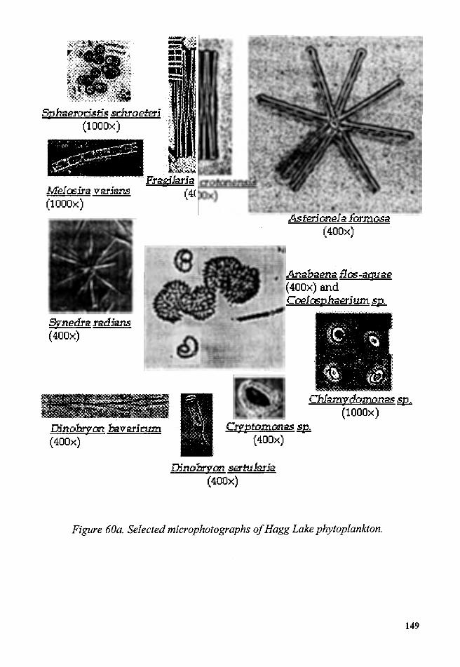
Sphae.rodstis sch.roeted (1000x)
Mel O!;i:ra varjan.s (1000x)
Synedra j'adjan.s (400x)
Fj'agilari a c::rofal:e. (400x)
As teri an.el a fcuomosa (400x)
Chlamydomonas & (1000x)
Dinobiyan ~varj cum (400x)
Czyptomanas ~ (400x)
Dinobiyan Si21'ftdarfa (400x)
Figure 60a. Selected microphotographs of Hagg Lake phytoplankton.
149
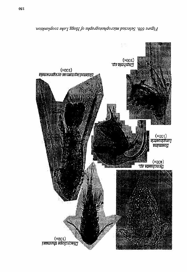
OSI
(xooi)
(xooi) =r:rew:=o=~= Sdop:<Gii.ra
(xooi)
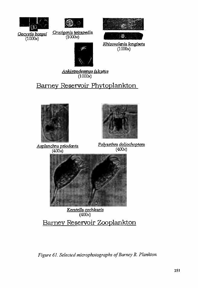
.. Ooc:;ystis borgei
(lOOOx) Crudgenia tetrapedia
(1000x)
Rhizosolenia Jongiseta (lOOOx)
Ankistrodesmus falcatus (lOOOx)
Barney Reservoir Phytoplankton
Asplandma priodanta (400x)
Polyarthra doliochoptera (400x)
Keratella cochlearis (400x)
Barney Reservoir Zooplankton
Figure 61. Selected microphotographs of Barney R. Plankton.
151

DISCUSSION
Conceptua!Afodel
A conceptual model was developed to identify the dimensions and
interacting factors that define a theoretical reservoir. Based on this model,
data from the variables measured were used to make inferences between the
interactions of the physical and chemical components and the effects or
responses of the plankton to these interactions.
PEGAfodel
The verbal model of plankton ecology group (PEG) was used to
describe the plankton dynamics in both Hagg Lake and Barney Reservoir.
This model, although suited to natural lakes, was a good predictor of the late
spring to late fall 1998 and spring 1999 planktonic successions (Figure 59).
PEG Af odel and Hagg Lake
The PEG model was used to describe the plankton dynamics in the
lacustrine zone of Hagg Lake (Figure 59). Statements 1 to 5: These statements
described the spring phytoplankton- herbivorous zooplankton dynamics. In
Hagg Lake what could be termed a 'clear phase' period (in the form of photic
152

zone depth) occurred in June 1998 and July 1999 with depths of around 7.5
m.
The statements 6 to 16 of the PEG model described the summer
planktonic succession. In Hagg Lake these statements apply, although in not
the same order. For example, as fish are used to stock the reservoir, the
impacts of its predation are perceptible through the decline of the large
bodied zooplankton (including the cyclopoids). However, unlike in natural
lakes, the decreases in water levels can cause a particular sequence to repeat
itself, as nutrients can be re-suspended while water temperatures are
relatively high or if light limitation caused by mixing-induced turbidity
occurs. In late summer, when most of the fish predation pressure is gone,
calanoids (grazers) biovolumes increased partly because the biovolumes of
adult cyclopoids were minimal. These large grazers can potentially out
compete smaller zooplankton. Thus, in the late summer of 1998,
phytoplankton species such as Dinobn;on sertularia, Chlamydomonas sp. and
Cryptomonas sp. increased providing support for a late summer population of
calanoids, bosminids, small Keratella sp., fast swimming Polyarthra sp. and big
transparent Synchaeta sp.
The statements 17 to 24 described the fall and winter planktonic
succession. For Hagg Lake the rainy season (November 1998 to March 1999)
153
causes increases in the inflows and the water storage of the reservoir.
Turbidity increases and the light regime deteriorates. The effects of these
physical changes are low photosynthesis and a decrease in the biovolumes of
the large-bodied zooplankton. During this period, Hagg Lake can be
described by two fall (17, 18) and three winter statements (21, 22, 23). It is
interesting to note that it was during the late winter period that the diversity
index for zooplankton was higher.
At the beginning of spring 1999 the waters stratified, and the
succession was started again with increases in biovolumes of small
phytoplankton and herbivorous zooplankters (Chlamydomonas sp.,
Cryptomonas sp. eucladocerans, copepods, and some rotifers).
PEG model and Barney Reservoir
The PEG model was used to describe the plankton dynamics in the
lacustrine zone of Barney Reservoir (Figure 59). The study period of Barney
Reservoir began at the time of the June 1998 clear-water phase, and ended at
the time of clear phase in 1999. The dominant species of the phytoplankton
by biovolume were colonial species rather than centric diatoms; daphnids
and rotifers dominated the herbivorous zooplankton succession. The
phytoplankton and zooplankton diversity were relatively high, particularly
after the Dinobryon sp. ceased to dominate the phytoplankton succession
(Statements 1-5).
154
In Barney Reservoir, the PEG statements 6to16 apply, although in not
the same order. Information on all the kinds of fish living in the reservoir
was not available and some fish predation on the zooplankton is suspected.
The dominance of daphnids (by biovolumes) decreased slowly during the
summer of 1998 and was replaced by the slight dominance of rotifers and
bosminids. Colonials (Chrysophytes and Chlorophytes) were replaced by
smaller cryptomonads and some colonial diatoms. The early start of the
period of mixing interrupted the planktonic succession, and non-colonial
species dominated the succession for the rest of the summer and early fall.
During this period of mixing (September 1998 to March 1999), Barney
Reservoir can be described by two of the PEG fall (17, 18) and two PEG
winter statements (21, 23). In Barney Reservoir, the early start of the period
of mixing together with the relatively high water temperatures and the re
suspension of nutrients allowed for a standing crop of cryptomonads and
other algae. These algae in turn appeared to sustain many rotifers, and these
in turn supported a population of predatory Asplanchna sp. (another rotifer).
With a decrease in temperatures, and increases in water volumes the
biovolumes of the zooplankton and phytoplankton diminished for the
remaining of the winter. Cryptomonads and Chlamydomonas were the
dominant phytoplankton groups; eucladocerans and a few rotifers were the
155

dominant phytoplankton groups; eucladocerans and a few rotifers were the
dominant zooplankton. In the spring of 1999 the reservoir stratified,
cryptomonads were replaced by colonial phytoplankton and the biovolumes
of the zooplankton increased again.
156
CONCLUSION
From June 1998 to July 1999, the dynamics of the plankton in Hagg
Lake and Barney Reservoir were studied through the identification of their
seasonal succession. The relationships between the planktonic successions
and the physical and chemical variables were explored with the aim of
identifying the abiotic conditions that could be used as indicators or
predictors of shifts in the successions of the plankton.
The close proximity between the two reservoirs and similar land soils
and vegetation cover within their watersheds justified the assumption of
similar species succession. However, the species that dominated the
successions (by biovolumes) in each reservoir were different.
Human activities in the form of agricultural and logging practices had
an impact on the turbidity and nutrient dynamics of Hagg Lake, particularly
during the summer season. The watershed of Barney Reservoir during the
study period had no permanent human settlements, logging or agricultural
activities. This reservoir also had a less variable nutrient dynamics and a
higher average photic zone depths.
A conceptual model was developed to identify the dimensions and
interacting factors that define a theoretical reservoir. Based on this model,
157
data from the variables measured were used to make inferences about the
interactions of the physical and chemical components and the effects or
responses of the plankton to these interactions. From the observations of
these interactions the following statements can be made:
1. Hagg Lake and Barney Reservoir have a mesotrophic lacustrine
zone.
2. Human impacts in the watershed (logging, road construction and
human habitation) of Hagg Lake have important consequences to the
nutrient and turbidity regimes at the sampling station, during the study
period. In Barney Reservoir the human impacts were almost non-existent
and this resulted in low but stable nutrient and turbidity regimes during the
study period.
Hagg Lake:
3. Dissolved oxygen in Hagg Lake appeared to be regulated by
changes in the water levels, and by the changing depth from the water
surface to the intake structure. Hypolimnetic anoxic conditions occurred in
the late summer at the same time withdrawals from the lower epilimnion
occurred.
4. Summer disturbances in the watershed of Hagg Lake that increased
the sediment loadings in the creeks that feed the reservoir, had a greater
impact on the turbidity than the normal winter loadings. However these
158
summer turbidity impacts were localized by the placements of the inflows
(according to the water temperature of the water of the creeks) in the water
column.
5. The concentrations of nutrients in Hagg Lake were low when
inflows were low, and increased as the rainy season progressed. Relatively
high concentrations of nutrients make Hagg Lake less likely to be under
nutrient stress than Barney Reservoir, despite the fact that according to the
TN:TP mass rations, Hagg Lake had slightly more instances of TN:TP mass
ratios less than 7 than Barney Reservoir did.
Barney Reservoir:
6. Changes in the water elevation influenced the temperature regime
of the water column of Barney Reservoir; the hypolimnetic waters warmed
as the water levels dropped, and could have caused temperature-related
anoxia.
7. The extreme differences between the highest and lowest water
levels had as consequence an early start of the long period of wind-induced
mixing (September 1998 to April 1999).
8. Low water levels caused re-suspension of nutrients in Barney
Reservoir. This was more noticeable in the case of total nitrogen
concentrations.
159
The PEG model was used to describe the plankton dynamics in both
reservoirs. This model, although suited to natural lakes, was a good
predictor of the late spring to late fall 1998 and spring 1999 planktonic
successions. Based on the fall 1998 to early spring 1999 discrepancies
between the predicted sequence and the observed succession two general
statements could be made.
1. In Hagg Lake, the high winter inflows and mixing caused by the
prevailing winds from the late fall to early spring weather systems, did not
allow a stable winter - spring succession. Species adapted to low light,
mixing, and low temperatures were common, and supported small and a few
large herbivorous zooplankton population. Predation by cyclopoids and fish
seemed to be the factors controlling the succession of the herbivorous
zooplankton in Hagg Lake.
2. The early start of mixing in Barney Reservoir interrupted the fall
succession as described in the PEG model, and a continuous resetting of the
succession favored population of cryptomonads, which sustained small
zooplankters. With increases in water volumes, lower temperatures and low
available light the biovolumes of the phytoplankton and zooplankton
decreased. If calanoids reach Barney Reservoir, they appear to be killed off
by the cyclopoids since planktivorous fish and insect larvae did not seem to
exert much predatory pressure on the cyclopoid population.
160

From the previous statements, I conclude that:
a) The development of conceptual models to identify the dimensions
and interacting factors that define a reservoir under study is not only useful
but should be a requirement if a more general model of planktonic dynamics
is to emerge.
b) The PEG model needs to be modified when applying it to
reservoirs. This is true for those periods when the water levels and water
volumes change dramatically such as during the period of winter storms or
late fall withdrawals. The PEG model needs to be modified to include
longitudinal variations in the concentrations of nutrients and the effects of
the convective and dispersive forces on the distribution of other variables as
water volumes change and synoptic cycles occur.
Finally, a hypothesis is put forth regarding the changes in plankton
dynamics should fish stocking be initiated in Barney Reservoir: as fish exert
more pressure on cyclopoids, calanoids will be able to colonize the reservoir.
In turn Dinobryon sp. or other grazing-resistant colonial algae, adapted to low
nutrients, will become more abundant, and the resulting succession will
resemble more closely the planktonic successions in Hagg Lake. If changes in
the land use practices occur, such as more human impact in the form of
161
settlements or clear-cutting of the forested areas, nutrient inputs and
turbidity will increase with a detrimental effect on the water quality of
Barney Reservoir.
162
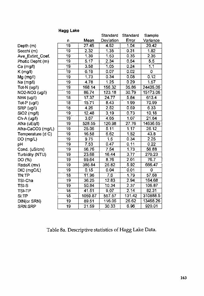
Depth (m) Secchi (m) Ave_Extint_Coef. Photic Depht (m) Ca (mg/I) K (mg/I) Mg (mg/I) Na (mg/I) Tot-N (ug/I) N02-N03 (ug/I) NH4 (ug/I) Tot-P (ug/I) SRP (ug/I) Si02 (mg/I) Ch-A (ug/I) Alka (uEq/I) Alka-CaC03 (mg/L) Temperature (d C) DO (mg/L) pH Cond. (uS/cm) Turbidity (NTU) DO(%) RedoX (mv) DIC (mgC/L) TN:TP TS I-Cha TSl-S TSl-TP Si:TP DIN( or SRN) SRN:SRP
Hagg Lake Standard Standard Sample
n Mean Deviation Error Variance 19 27.45 4.52 1.04 20.42 19 2.32 1.35 0.31 1.82 19 1.39 1.53 0.35 2.35 19 5.17 2.34 0.54 5.5 19 3.58 1.05 0.24 1.1 19 0.19 0.07 0.02 0 19 1.73 0.34 0.08 0.12 19 4.78 1.25 0.29 1.57 19 168.14 156.32 35.86 24435.06 16 86.74 123.18 30.79 15173.06 18 17.37 24.77 5.84 613.4 18 15.71 8.43 1.99 70.99 18 4.26 2.52 0.59 6.33 19 12.48 3.19 0.73 10.18 19 3.67 4.65 1.07 21.64 19 528.55 120.98 27.76 14636.65 19 25.06 5.11 1.17 26.12 19 16.58 6.62 1.52 43.8 19 9.75 1.5 0.34 2.25 19 7.53 0.47 0.11 0.22 19 56.76 7.54 1.73 56.88 19 23.68 16.44 3.77 270.23 19 99.64 8.76 2.01 76.7 19 386.84 25.82 5.92 666.47 19 0.15 0.04 0.01 0 18 11.96 7.6 1.79 57.68 19 36.25 12.83 2.94 164.68 19 50.84 10.34 2.37 106.87 18 41.51 9.07 2.14 82.31 18 1059.87 557.57 131.42 310888.5 19 89.51 116.05 26.62 13468.26 19 21.59 30.33 6.96 920.01
Table Sa. Descriptive statistics of Hagg Lake Data.
163

Depth (m) Secchi (m) Ave_Extint_Coef. Photic Depht (m) Ca (mg/I) K (mg/I) Mg (mg/I) Na (mg/I) Tot-N (ug/I) N02-N03 (ug/I) NH4 (ug/I) Tot-P (ug/I) SRP (ug/I) Si02 (mg/I) Ch-A (ug/I) Alka (uEq/I) Alka-CaC03 (mg/L) Temperature (d C) DO (mg/L) pH Cond. (uS/cm) Turbidity (NTU) DO(%) RedoX (mv) DIC (mgC/L) TN:TP TS I-Cha TSl-S TSl-TP Si:TP DIN( or SRN) SRN:SRP
Hagg Lake Range 95% Cont.
Median Kurtosis Skewness Minimum Maximum Level 28.5 -1.38 -0.31 20 33.5 2.18 2.1 -0.5 0.46 0.4 5 0.65
0.78 11.99 3.28 0.54 7.15 0.74 5.88 -0.88 -0.49 0.64 8.56 1.13 3.46 -1.27 -0.15 1.8 5.21 0.5 0.18 -0.54 0.34 0.09 0.34 0.03 1.66 0.13 0.6 1.19 2.45 0.16 4.99 -1.39 -0.18 2.79 6.52 0.6 105.9 5.6 2.31 61.87 671.43 75.34 10.95 -0.7 1.05 0.13 329.47 65.64 7.5 4.44 2.34 2.73 82.43 12.32 15.4 -0.51 0.39 4.04 33.5 4.19 4.11 2.21 1.27 0.75 11.23 1.25 13.03 2.35 0.53 6.53 21.11 1.54 2.18 1.54 1.7 0.12 14.76 2.24 499.2 0.39 0.96 378.8 820 58.31 23.58 0.07 0.76 17.84 36.75 2.46 17.87 -1.32 -0.39 5.77 25.28 3.19 9.56 -1.51 0.24 7.57 12.16 0.72 7.54 0.03 0.64 6.88 8.55 0.23 59.3 -0.55 -0.27 42.6 70.5 3.64 18 -0.84 0.59 2 57 7.92
96.9 3.83 1.56 88.6 126.4 4.22 386 0.65 0.86 349 449 12.44 0.14 -0.81 0.4 0.09 0.21 0.02 10.25 -0.35 0.77 3.23 28.02 3.78 38.21 0.02 -0.18 9.77 56.98 6.19 49.3 -0.34 0.71 36.78 73.22 4.98 43.59 -0.79 -0.54 24.29 54.81 4.51
911.44 -0.18 0.71 194.93 2293.28 277.28 20.22 -0.07 1.23 1.13 332.2 55.94 5.01 3.13 1.85 0.36 109.91 14.62
Table Sa. Descriptive statistics of Hagg Lake Data (cont.).
164
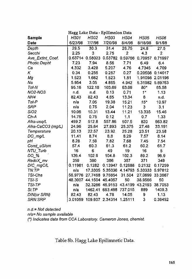
Hagg Lake Data - Epilimnion Data Sample HS01 HS02 HS03 HS04 HS05 HS06 Date 6/23/98 7/7/98 7/20/98 8/4/98 8/18/98 9/1/98 Depth 29.5 30.3 31.4 26.75 24.8 27.5 Secchi 2.25 3 2.75 2 4.3 2 Ave_Extint_ Coef. 0.63714 0.58023 0.53782 0.59766 0.70957 0.71997 Photic Oepht 7.23 7.94 8.56 7.71 6.49 6.4 Ca 4.332 3.428 5.207 4.76 4.7345 4.709 K 0.34 0.255 0.257 0.27 0.20508 0.14017 Mg 1.523 1.662 1.523 1.81 1.91098 2.01196 Na 5.954 3.05 4.865 4.942 5.31982 5.69763 Tot-N 95.16 122.18 103.69 63.09 80* 65.58 N02-N03 n.d. n.d. 0.13 0.71 1* 1.13 NH4 82.43 82.43 4.65 13.34 8 n.d. Tot-P n/a 7.05 19.38 15.21 15* 10.97 SRP n/a 0.75 2.04 11.23 3 3.1 Si02 10.06 10.31 13.44 11.21 13.335 15.46 Ch-A 14.76 0.75 0.12 1.1 0.7 1.33 Alka-ueq/L 499.2 512.8 557.86 507.5 820 663.82 Alka-CaC03 (mg/L) 24.96 25.64 27.893 25.375 27.48 33.191 Temperature 20.13 22.57 23.92 25.28 23.51 23.58 OO_mg/L 11.41 8.74 8.8 8.29 7.57 8.14 pH 8.28 7.59 7.82 7.68 7.45 7.54 Cond_uSlcm 57.4 60.3 61.3 61.2 60.2 61.7 NTU_Turb 16 6 49 19 16 5 00_% 126.4 102.9 104.8 102.3 89.2 96.9 RedoX_mv 359 380 386 357 371 349 OIC_mgC/L 0.11981 0.1282 0.13947 0.12688 0.2132 0.17259 TN:TP n/a 17.3305 5.35036 4.14793 5.33333 5.97812 TS I-Cha 56.9776 27.7468 9.76854 31.504 27.0699 33.3667 TSl-S 48.3007 44.1504 45.4057 50 38.9566 50 TSl-TP n/a 32.3266 46.9153 43.4199 43.2193 38.7053 Si:TP n/a 1462.41 693.498 737.015 889 1409.3 DIN(orSRN) 82.43 82.43 4.78 14.05 9 1.13 SRN:SRP 3.01059 109.907 2.34314 1.25111 3 0.36452
n.d.= Not detected nla= No sample available (j Indicates data from CCA Laboratory. Cameron Jones, chemist.
Table 8b. Hagg Lake Epilimnetic Data.
165
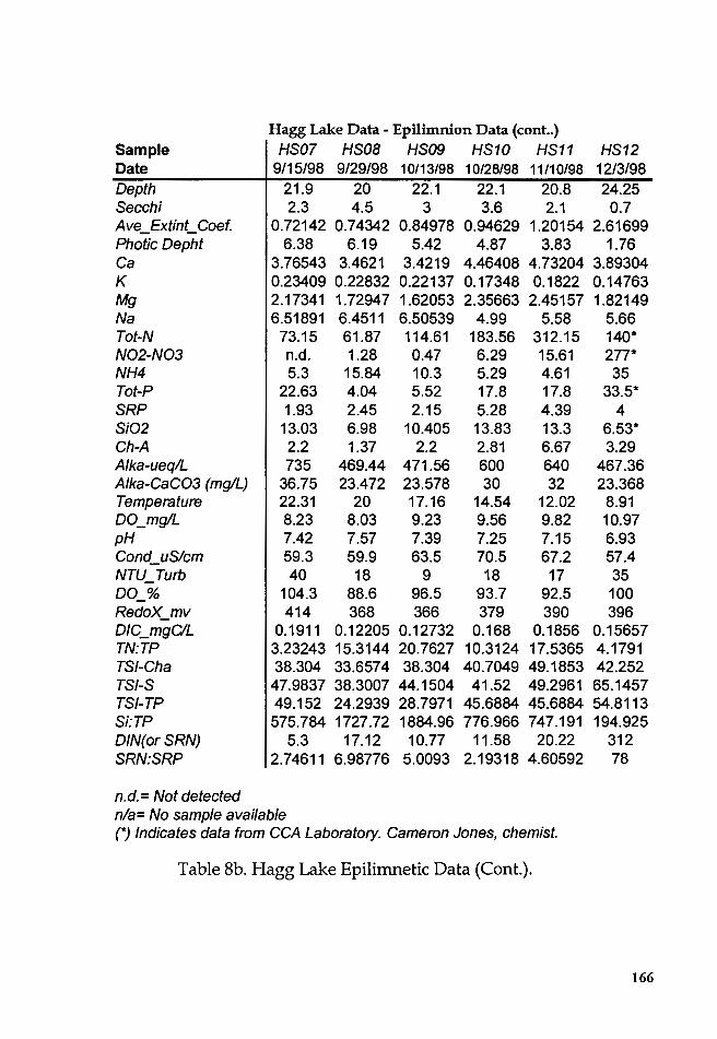
Sample Date Depth Secchi Ave_ExtinLCoef. Photic Depht Ca K Mg Na Tot-N N02-N03 NH4 Tot-P SRP Si02 Ch-A Alka-ueq!L Alka-CaC03 (mg/L) Temperature DO_mg/L pH Cond_uS/cm NTU_Turb 00_% RedoX_mv DIC_mgC/L TN:TP TS I-Cha TSl-S TSl-TP Si:TP DIN(orSRN) SRN:SRP
n.d.= Not detected
Hagg Lake Data - Epilimnion Data (cont .. ) HS07 HSOB HS09 HS10 HS11 HS12
9/15/98 9/29/98 10/13/98 10/28/98 11/10/98 12/3/98 21.9 20 22.1 22.1 20.8 24.25 2.3 4.5 3 3.6 2.1 0.7
0.72142 0.74342 0.84978 0.94629 1.20154 2.61699 6.38 6.19 5.42 4.87 3.83 1. 76
3.76543 3.4621 3.4219 4.46408 4.73204 3.89304 0.23409 0.22832 0.22137 0.17348 0.1822 0.14763 2.17341 1.72947 1.62053 2.35663 2.45157 1.82149 6.51891 6.4511 6.50539 4.99 5.58 5.66
73.15 61.87 114.61 183.56 312.15 140* n.d. 1.28 0.4 7 6.29 15.61 277* 5.3 15.84 10.3 5.29 4.61 35
22.63 4.04 5.52 17.8 17.8 33.5* 1.93 2.45 2.15 5.28 4.39 4 13.03 6.98 10.405 13.83 13.3 6.53* 2.2 1.37 2.2 2.81 6.67 3.29 735 469.44 471.56 600 640 467.36
36.75 23.472 23.578 30 32 23.368 22.31 20 17.16 14.54 12.02 8.91 8.23 8.03 9.23 9.56 9.82 10.97 7.42 7.57 7.39 7.25 7.15 6.93 59.3 59.9 63.5 70.5 67.2 57.4 40 18 9 18 17 35
104.3 88.6 96.5 93. 7 92.5 100 414 368 366 379 390 396
0.1911 0.12205 0.12732 0.168 0.1856 0.15657 3.23243 15.3144 20.7627 10.3124 17.5365 4.1791 38.304 33.6574 38.304 40.7049 49.1853 42.252
47.9837 38.3007 44.1504 41.52 49.2961 65.1457 49.152 24.2939 28.7971 45.6884 45.6884 54.8113 575.784 1727.72 1884.96 776.966 747.191 194.925
5.3 17.12 10.77 11.58 20.22 312 2.74611 6.98776 5.0093 2.19318 4.60592 78
nla= No sample available (*) Indicates data from CCA Laboratory. Cameron Jones, chemist.
Table Sb. Hagg Lake Epilimnetic Data (Cont.).
166

Hagg Lake Data - Epilimnion Data (cont .. ) Sample HS13 HS14 HS15 HS16 HS17 HS18 HS19 Date 1/19/99 2/17/99 3/16/99 4/14/99 5/12/99 5/26/99 6/16/99 Depth 28.5 29.3 31.55 33.2 33.5 31.7 32.45 Secchi 0.75 0.7 0.4 0.9 1.75 2 5 Ave_Extint_ Coef. 2.51592 2.01307 7.14989 1.44312 1.06641 0.78313 0.62801 Photic Depht 1.83 2.29 0.64 3.19 4.32 5.88 7.33 Ca 3.37 1.79863 2.15515 2.34923 2.42749 2.63127 2.47388 K 0.166 0.26312 0.14183 0.1006 0.12299 0.11362 0.091 Mg 1.68 1.27725 1.18978 1.5457 4 1.63889 1.26998 1.60846 Na 5.09 2.78944 3.26136 3.69675 3.59757 3.56891 3.3204 Tot-N 208.19 222.4 671.43 436.5 105.9 65.97 69.21 N02-N03 329.47 268.58 241.55 169.71 53.38 5.78 15.78 NH4 2.73 5.81 6.99 4.62 9 11.54 4.86 Tot-P 26.98 21.83 26.14 15.58 7.33 4.91 11.04 SRP 7.22 6.01 7.29 4.57 4.22 4.65 2.45 Si02 14.6 21.11 13.98 14.55 12.14 11.26 11.62 Ch-A 0.56 0.19 2.18 13.1 12.84 2.53 1.1 Alka-ueq!L 421.1 606.1 455 383.68 378.8 425.2 428 Alka-CaC03 (mg!L) 21.105 17.842 22.75 19.184 18.94 21.26 21.4 Temperature 6.03 5.77 7.11 10.64 13.02 17.87 20.73 DO_mg/L 11.4 11.73 11.6 12.16 11.22 9.59 8.67 pH 6.88 6.91 7.03 8.31 8.55 7.72 7.54 Cond_uS!cm 49.4 45.3 42.6 46.3 51 52.5 51.5 NTU_Turb 45 39 57 35 8 16 2 00_% 91.8 93.7 95.9 109.4 106.5 101.1 96.7 RedoX_mv 407 449 433 387 393 368 398 DIC_mgC/L 0.15581 0.20607 0.14333 0.09208 0.0947 0.1063 0.11128 TN:TP 7.71646 10.1878 25.6859 28.0167 14.4475 13.4358 6.26902 TS I-Cha 24.8808 14.2767 38.2145 55.8072 55.6105 39.6752 31.504 TS/-S 64.1504 65.1457 73.2193 61.52 51.9265 50 36.7807 TSl-TP 51.6886 48.6328 51.2322 43.7666 32.8885 27.1076 38.7971 Si:TP 541.142 967.018 534.813 933.89 1656.21 2293.28 1052.54 DIN(orSRN) 332.2 274.39 248.54 174.33 62.38 17.32 20.64 SRN:SRP 46.0111 45.6556 34.0933 38.1466 14.782 3.72473 8.42449
Table Sb. Hagg Lake Epilimnetic Data (Cont.).
167
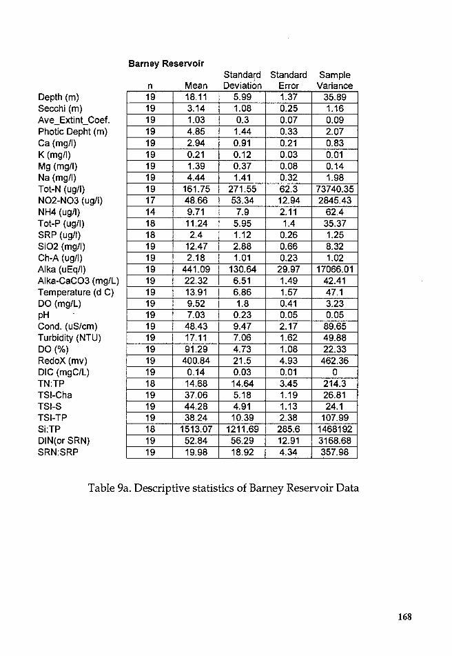
Depth (m) Secchi (m) Ave_Extint_Coef. Photic Depht (m) Ca (mg/I) K (mg/I) Mg (mg/I) Na (mg/I) Tot-N (ug/I) N02-N03 (ug/I) NH4 (ug/I) Tot-P (ug/I) SRP (ug/I) Si02 (mg/I) Ch-A (ug/I) Alka (uEq/I) Alka-CaC03 (mg/L) Temperature (d C) DO (mg/L) pH Cond. (uS/cm) Turbidity (NTU) DO(%) RedoX (mv) DIC (mgC/L) TN:TP TS I-Cha TSl-S TSl-TP Si:TP DIN( or SRN) SRN:SRP
Barney Reservoir Standard Standard Sample
)
n Mean Deviation Error Variance 19 18.11 5.99 1.37 35.89 19 3.14 1.08 0.25 1.16 19 1.03 0.3 0.07 0.09 19 4.85 1.44 0.33 2.07 19 2.94 0.91 0.21 0.83 19 0.21 0.12 0.03 0.01 19 1.39 0.37 0.08 0.14 19 4.44 1.41 0.32 1.98 19 161.75 271.55 62.3 73740.35 17 48.66 53.34 12.94 2845.43 14 9.71 7.9 2.11 62.4 18 11.24 5.95 1.4 35.37 18 2.4 1.12 0.26 1.25 19 12.47 2.88 0.66 8.32 19 2.18 1.01 0.23 1.02 19 441.09 130.64 29.97 17066.01 19 22.32 6.51 1.49 42.41 19 13.91 6.86 1.57 47.1 19 9.52 1.8 0.41 3.23 19 7.03 0.23 0.05 0.05 19 48.43 9.47 2.17 89.65 19 17.11 7.06 1.62 49.88 19 91.29 4.73 1.08 22.33 19 400.84 21.5 4.93 462.36 19 0.14 0.03 0.01 0 18 14.68 14.64 3.45 214.3 19 37.06 5.18 1.19 26.81 19 44.28 4.91 1.13 24.1 19 38.24 10.39 2.38 107.99 18 1513.07 1211.69 285.6 1468192 19 52.84 56.29 12.91 3168.68 19 19.98 18.92 4.34 357.98
Table 9a. Descriptive statistics of Barney Reservoir Data
168
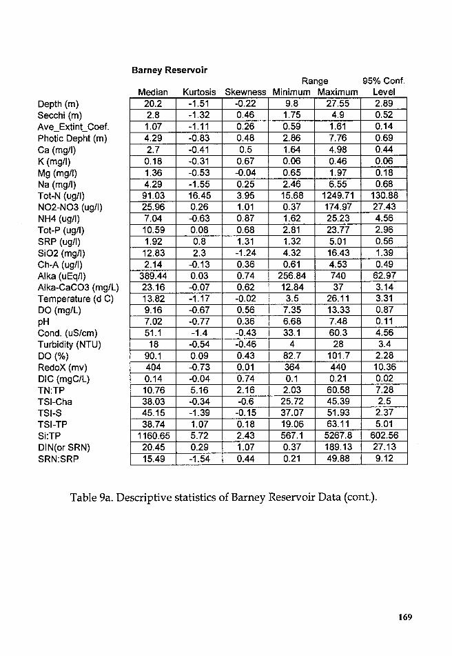
Depth (m) Secchi (m) Ave_Extint_Coef. Photic Depht (m) Ca (mg/I) K (mg/I) Mg (mg/I) Na (mg/I) Tot-N (ug/I) N02-N03 (ug/I) NH4 (ug/I) Tot-P (ug/I) SRP (ug/I) Si02 (mg/I) Ch-A (ug/I) Alka (uEq/I) Alka-CaC03 (mg/L) Temperature (d C) DO (mg/L) pH Cond. (uS/cm) Turbidity (NTU) DO(%) RedoX (mv) DIC (mgC/L) TN:TP TS I-Cha TSl-S TSl-TP Si:TP DIN( or SRN) SRN:SRP
Barney Reservoir Range 95% Conf.
Median Kurtosis Skewness Minimum Maximum Level 20.2 -1.51 -0.22 9.8 27.55 2.89 2.8 -1.32 0.46 1.75 4.9 0.52 1.07 -1.11 0.26 0.59 1.61 0.14 4.29 -0.83 0.48 2.86 7.76 0.69 2.7 -0.41 0.5 1.64 4.98 0.44 0.18 -0.31 0.67 0.06 0.46 0.06 1.36 -0.53 -0.04 0.65 1.97 0.18 4.29 -1.55 0.25 2.46 6.55 0.68 91.03 16.45 3.95 15.68 1249.71 130.88 25.96 0.26 1.01 0.37 174.97 27.43 7.04 -0.63 0.87 1.62 25.23 4.56 10.59 0.08 0.68 2.81 23.77 2.96 1.92 0.8 1.31 1.32 5.01 0.56 12.83 2.3 -1.24 4.32 16.43 1.39 2.14 -0.13 0.36 0.61 4.53 0.49
389.44 0.03 0.74 256.84 740 62.97 23.16 -0.07 0.62 12.84 37 3.14 13.82 -1.17 -0.02 3.5 26.11 3.31 9.16 -0.67 0.56 7.35 13.33 0.87 7.02 -0.77 0.36 6.68 7.48 0.11 51.1 -1.4 -0.43 33.1 60.3 4.56 18 -0.54 -0.46 4 28 3.4
90.1 0.09 0.43 82.7 101.7 2.28 404 -0.73 0.01 364 440 10.36 0.14 -0.04 0.74 0.1 0.21 0.02 10.76 5.16 2.16 2.03 60.58 7.28 38.03 -0.34 -0.6 25.72 45.39 2.5 45.15 -1.39 -0.15 37.07 51.93 2.37 38.74 1.07 0.18 19.06 63.11 5.01
1160.65 5.72 2.43 567.1 5267.8 602.56 20.45 0.29 1.07 0.37 189.13 27.13 15.49 -1.54 0.44 0.21 49.88 9.12
Table 9a. Descriptive statistics of Barney Reservoir Data (cont.).
169
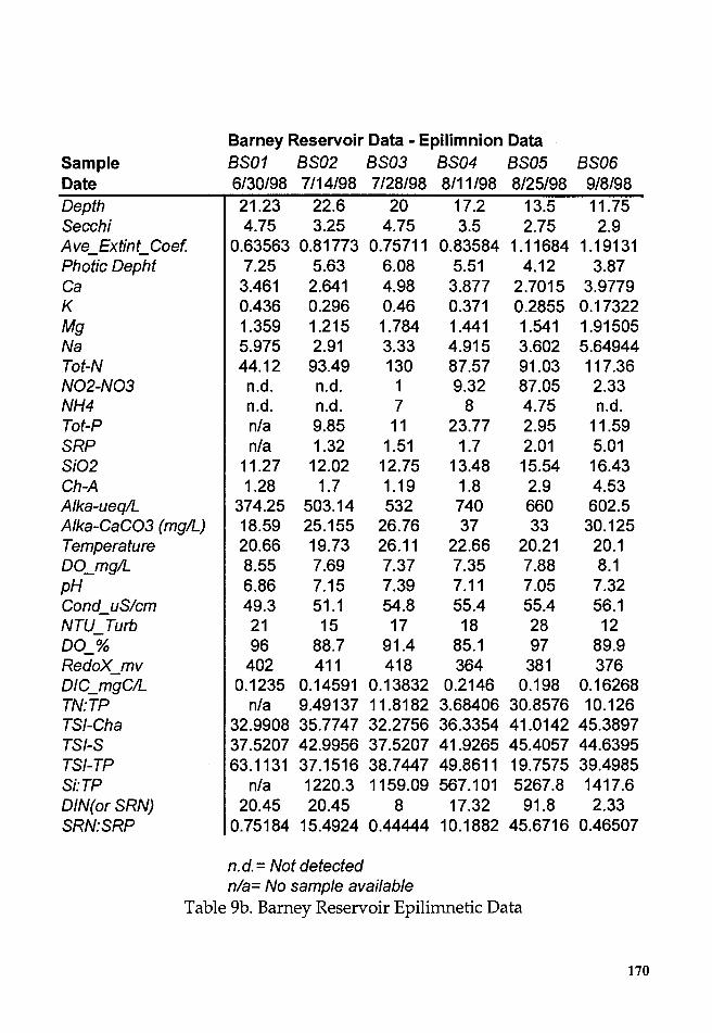
Barney Reservoir Data - Epilimnion Data Sample BS01 BS02 BS03 BS04 BS05 BS06 Date 6/30/98 7 /14/98 7 /28/98 8/11 /98 8/25/98 9/8/98 Depth 21.23 22.6 20 17.2 13.5 11.75 Secchi 4.75 3.25 4.75 3.5 2.75 2.9 Ave_Extint_Coef. 0.63563 0.81773 0.75711 0.83584 1.11684 1.19131 Photic Depht 7.25 5.63 6.08 5.51 4.12 3.87 Ca 3.461 2.641 4.98 3.877 2.7015 3.9779 K 0.436 0.296 0.46 0.371 0.2855 0.17322 Mg 1.359 1.215 1.784 1.441 1.541 1.91505 Na 5.975 2.91 3.33 4.915 3.602 5.64944 Tot-N 44.12 93.49 130 87.57 91.03 117.36 N02-N03 n.d. n.d. 1 9.32 87.05 2.33 NH4 n.d. n.d. 7 8 4.75 n.d. Tot-P n/a 9.85 11 23.77 2.95 11.59 SRP n/a 1.32 1.51 1.7 2.01 5.01 Si02 11.27 12.02 12.75 13.48 15.54 16.43 Ch-A 1.28 1.7 1.19 1.8 2.9 4.53 Alka-ueq/L 374.25 503.14 532 740 660 602.5 Alka-CaC03 (mg/L) 18.59 25.155 26.76 37 33 30.125 Temperature 20.66 19.73 26.11 22.66 20.21 20.1 DO_mg!L 8.55 7.69 7.37 7.35 7.88 8.1 pH 6.86 7.15 7.39 7.11 7.05 7.32 Cond_uS/cm 49.3 51.1 54.8 55.4 55.4 56.1 NTU_Turb 21 15 17 18 28 12 00_% 96 88.7 91.4 85.1 97 89.9 RedoX_mv 402 411 418 364 381 376 DIC_mgCIL 0.1235 0.14591 0.13832 0.2146 0.198 0.16268 TN:TP n/a 9.49137 11.8182 3.68406 30.8576 10.126 TS I-Cha 32.9908 35.7747 32.2756 36.3354 41.0142 45.3897 TSl-S 37.5207 42.9956 37.5207 41.9265 45.4057 44.6395 TSl-TP 63.1131 37.1516 38.7447 49.8611 19.7575 39.4985 Si:TP n/a 1220.3 1159.09 567.101 5267.8 1417.6 DIN(orSRN) 20.45 20.45 8 17.32 91.8 2.33 SRN:SRP 0.75184 15.4924 0.44444 10.1882 45.6716 0.46507
n.d.= Not detected nla= No sample available
Table 9b. Barney Reservoir Epilimnetic Data
170

Barney Reservoir Data - Epilimnion Data (cont.)
Sample BS07 BSOB BS09 BS10 BS11 BS12 BS13 Date 9/22/98 10/6/98 10/20/98 11/3/98 11/17/98 12/10/98 1/12/99 Depth 10.9 9.8 10.6 10.3 10.4 20.2 24.7 Secchi 2.2 2 1.75 2.5 2.8 2.25 2 Ave_Extint_ Coef. 1.60809 1.3846 1.39279 1.276 1.35273 1.07404 1.28052 Photic Depht 2.86 3.33 3.31 3.61 3.4 4.29 3.6 Ca 3.21091 3.24912 3.02682 3.98135 3.94899 2.51998 2.4 K 0.27793 0.2652 0.24744 0.17985 0.17094 0.17227 0.131 Mg 1.70854 1.52248 1.52104 1.97219 1.9531 1.24177 1.17 Na 6.42726 6.54775 6.48294 5.31 5.9 4.57 4.29 Tot-N 56.46 97.41 145.65 176.85 1249.71 81.81 79.88 N02-N03 6.89 14.36 58 67.1 119.43 174.97 124.84 NH4 2.74 n.d. 20.8 14.13 25.23 14.16 7.07 Tot-P 21.18 6.27 8.5 14.17 20.63 11.59 9.98 SRP 1.63 2.45 1.85 3.79 2.9 4.68 3.18 Si02 14.8 4.32 8.6 15.39 15.34 13.47 12.83 Ch-A 3.06 3.06 3.05 2.91 2.67 0.61 1.9 Alka-ueq!L 389.44 514.4 463.2 471.47 500 311.56 290.52 Alka-CaC03 (mg/L) 19.472 25.72 23.16 23.55 25 15.578 14.526 Temperature 18.15 16.3 12.4 10.33 8.45 5.08 3.94 DO_mg!L 7.4 8.88 9.4 9.75 10.73 12.11 13.33 pH 6.94 7.29 7.04 6.87 6.92 6.69 6.86 Cond_uS/cm 55.3 58.4 60.3 58.8 57.2 38.5 34.8 NTU_Turb 20 19 25 18 6 26 25 00_% 82.7 90.1 87.4 86.8 93 98.3 101.7 RedoX_mv 376 371 414 401 393 407 404 D/C_mgCIL 0.12267 0.14403 0.14359 0.16501 0.1675 0.12462 0.10895 TN:TP 2.66572 15.5359 17.1353 12.4806 60.5773 7.05867 8.00401 TS I-Cha 41.541 41.541 41.5089 41.048 40.2035 25.7198 36.8658 TS/-S 48.625 50 51.9265 46. 7807 45.1457 48.3007 50 TSl-TP 48.1967 30.635 35.025 42.3981 47.8171 39.4985 37.3408 Si:TP 698.772 688.995 1011.76 1086.1 743.577 1162.21 1285.57 DIN(orSRN) 9.63 14.36 78.8 81.23 144.66 189.13 131.91 SRN:SRP 5.90798 5.86122 42.5946 21.4327 49.8828 40.4124 41.4811
Table 9b. Barney Reservoir Epilimnetic Data (Cont.).
171

Sample Date Depth Secchi Ave_Extint_Coef. Photic Depht Ca K Mg Na Tot-N N02-N03 NH4 Tot-P SRP Si02 Ch-A Alka-ueq!L Alka-CaC03 (mg/L) Temperature DO_mg/L pH Cond_uS/cm NTU_Turb 00_% RedoX_mv DIC_mgC/L TN:TP TS I-Cha TSl-S TSl-TP Si:TP DIN(orSRN) SRN:SRP
Barney Reservoir Data - Epilimnion Data (cont.) BS14 BS15 BS16 BS17 BS18 BS19 2123199 3/23/99 4121199 5/19/99 an 199 1n199 27.55 25.3 21.3 23.1 2.05 2.55 4.9 4
1.08318 0.88652 0.79418 0.72471 4.25 5.19 5.8 6.35
22.6 4.4
0.7695 5.98
21 4.4
0.59334 7.76
1.64248 1.78022 1.86245 2.07206 2.30139 2.31274 0.18336 0.07333 0.06198 0.09533 0.06988 0.11135 0.64735 0.92065 1.24142 1.24573 1.04433 0.98637 2.45782 3.02319 2.94724 3.57551 3.29347 3.18156
57.48 256.32 237.24 31.99 15.68 23.2 71.78 60.74 25.96 1.44 1.59 0.37 3. 79 20.82 3.36 2.41 1.62 n.d. 10.18 7.11 14.58 2.81 4.64 11.44 2.77 1.71 1.5 1.98 1.4 1.74 13.93 11.91 13.36 11.26 9.36 10.78 1.04 2.49 2.14 2.98 0.86 1.29
256.84 380 309.46 345.2 360 376.8 12.842 24 15.473 17.26 18 18.84
3.5 5.67 8.88 11.2 13.82 17.08 11.84 11.37 10.89 10.34 9.16 8.67 6.76 6.68 6.87 7.02 7.24 7.48 33.5 33.1 37 .6 41. 7 44.3 44.5 11 22 5 4 19 14
89.2 90.6 93.9 94.2 88.6 89.9 440 427 434 409 406 382
0.1053 0.1672 0.11295 0.10701 0.1008 0.09797 5.64637 36.0506 16.2716 11.3843 3.37931 2.02797 30.9538 39.5188 38.0328 41.2811 29.0894 33.0671 49.6438 46.495 37.0722 40 38.625 38.625 37.627 32.4489 42.8096 19.0561 26.2916 39.3105 1368.37 1675.11 916.324 4007.12 2017.24 942.308 75.57 81.56 29.32 3.85 3.21 0.37
27.2816 47.6959 19.5467 1.94444 2.29286 0.21264
Table 9b. Barney Reservoir Epilimnetic Data (Cont.).
172
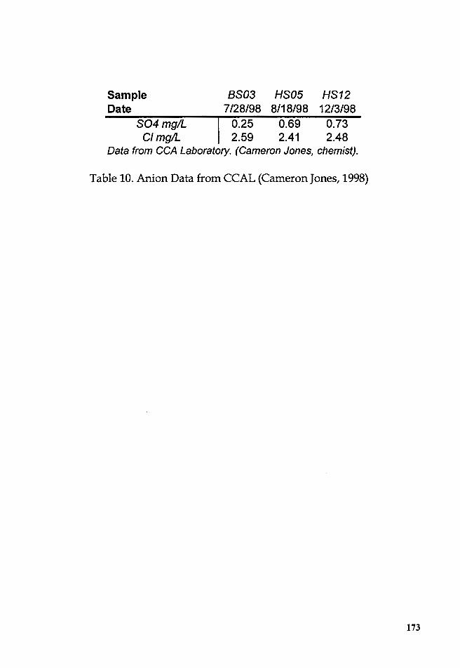
Sample BS03 HS05 HS12 Date 7 /28/98 8/18/98 12/3/98
S04 mg!L I 0.25 0.69 0. 73 Cl mg!L 2.59 2.41 2.48
Data from CCA Laboratory. (Cameron Jones, chemist).
Table 10. Anion Data from CCAL (Cameron Jones, 1998)
173
REFERENCES
Ameel, J. J. Ameel, Axler, R. P., Owen, C. J. 1995. Persulfate digestion for determination of total nitrogen and phosphorus in low-nutrient waters. Am. Env. Lab. 5(6), 4 pages.
American Public Health Association. 1995. Standard Methods for the Examination of Water and Wastewater. 19th Ed. American Public Health Association, Washington, DC. 1555 pp.
Axler, R. P., Owen, C. J. 1994. Measuring chlorophyll and phaeophytin: Whom should you believe? Lake and Reserv. Manage. 8(2):143-151.
Beaty R. D., Kerber, J. D. 1993. Concepts, instrumentation and techniques in atomic adsorption spectrophotometry. The Perkin-Elmer Corp., Norwalk, Connecticut.
Cameron Jones, 1998. Cooperative Central Analytical Laboratory, sample collection, handling and preservation document. Personal communication.
Carlson, R. E. 1977. A trophic state index for lakes. Limnol. and Ocean. 22:361-369
Carpenter, K. D. 1994. Indicators of nutrient limited plankton growth in lakes near mount Saint Helens, WA. M.S. Thesis, Portland State University. 175 pp.
Contant, H. and Duthie, H.C. 1978. The phytoplankton of Lac St-Jean, Quebec. (Bibliotheca Phycologica, Band 40). J. Cramer-Strauss and Cramer GmbH, Hirsheberg II, Germany. 165 pp (30 Plates).
Corliss, John Ozro, 1979. The ciliated protozoa, characterization, classification and guide to the literature. 2nd. Ed., Pergamon Press Ltd., New York, New York. 455 pp.
174
Honea, J.M. (1997). The periphyton community of a second order subalpine stream following salmon carcass decomposition: a potential facilitator of energy flow from adult to juvenile salmonids. Portland State University M.A. Thesis, 52pp.
Huber-Pestalotz, G., 1941. Das Phytoplankton des SillSwassers, sistematik und Biologie. Die Binnengewasser Limnologie und ihren Nachbargebieten, Band XVI, 2 Teil, Stuggart, Germany.
Johnson, D. M., Petersen, R. P., Lycan, R. D., Sweet, J. W., Neuhaus, M.E., Schaedel A. L. 1985. Atlas of Oregon Lakes. Oregon State University Press, Corvallis, Oregon.
Jones, M. N. 1984. Nitrate reduction by shaking with cadmium, alternative to cadmium columns. Water Res. 18(5):643-646.
Knutson, M. T. 1993. Modelling of flow and water quality in Henry Hagg Lake near Forest Grove, Oregon. M.S. Thesis, Portland State University. 146 pp.
Krammer, K. and Lange-Bertalot, H. 1991. Bacillariophyceae 1., Herausgegeben von H. et al. Ed. Band 2/1. SillSwasserflora von Mitteleuropa. Gustav Fisher Verlag. Stuttgart, Germany.
Krammer, K. and Lange-Bertalot, H. 1991. Bacillariophyceae 2., Herausgegeben von H. et al. Ed. Band 2/ 2. SillSwasserflora von Mitteleuropa. Gustav Fisher Verlag. Stuttgart, Germany.
Krammer, K. and Lange-Bertalot, H. 1991. Bacillariophyceae 3., Herausgegeben von H. et al. Ed. Band 2/3. SillSwasserflora von Mitteleuropa. Gustav Fisher Verlag. Stuttgart, Germany.
Krammer, K. and Lange-Bertalot, H. 1991. Bacillariophyceae 4., Herausgegeben von H. et al. Ed. Band 2/ 4. SillSwasserflora von Mitteleuropa. Gustav Fisher Verlag. Stuttgart, Germany.
Lewis, T.H. and Britton, M.E., 1971. The Algae of Illinois. Hafner Publishing Co., New York, N. Y.
Nauwerck, A. 1963. Die Beziehungen zwischen Zooplankton und Phytoplankton im See Erken. Symbol. Bot. Upsaliensis 17(5):1-163.
175
Patrick, R. and Reimer, C. W., 1966. The Diatoms of the United States Exclusive of Alaska and Hawaii. Vol. I and II. Monographs of the Academy of Natural Sciences of Philadelphia. No. 13. Livingston Publishing Co. Philadelphia.
Pennak, R. W. 1989. Fresh-Water invertebrates of the United States: Protozoa to Mollusca. 3rd. Edition. Wiley and Sons, Pub. New York.
Prescott, G.W. 1978. How to Know the Freshwater Algae. 3rd. Edition. Wm. C. Brown Co. Publishers. Dubuque, Iowa, USA.
Prescott, G.W., 1962. Algae of the Western Great Lakes Area. Cranbrook Institute of Science, Bulletin No. 31., Reprint 1982 by Otto Koeltz Science Publishers. Koenigstein. W. Germany.
Reynolds, C.S. 1996. The plant life of the pelagic. Verh. Internat. Verein. Limnol. 26:97-113.
Reynolds, C. S. 1984. The ecology of Freshwater Phytoplankton. Cambridge University Press. Cambridge, Great Britain.
Ryder, R. A. 1978. Ecological heterogeneity between north-temperate reservoirs and glacial lakes systems due to different succession rates and cultural uses. Verh. Int. Verein. Limnol. 20:1568-1574.
Shannon C. E. and Weaver W. 1949. The mathematical theory of communication. The University of Illinois Press. Urbana, Illinois.
Smith, G.M., 1950. The Freshwater Algae of the United States. 2nd. Edition. McGraw-Hill Book Co. New York, N.Y., USA.
Sternberger, R. S. 1979. A Guide to Rotifers of the Laurentian Great Lakes. EPA-600/4-79-021. Environmental monitoring and support laboratory. U.S. Environmental Protection Agency. Cincinnati, Ohio, U.S.A.
176
Stewart, A.R. 1980. Relationships between trout and invertebrate species as predators and the structure of the crustaceans and rotiferans plankton in Mountain Lakes (625-634). Herfoot, W.C. Editor. Evolution and Ecology of Zooplankton Communities, University Press of New England, New Hampshire, U.S.A.
Sommer U. 1993. Disturbance diversity relationships in two lakes of similar nutrient chemistry but contrasting disturbance regimes. Hydrobiologia 249: 59-65.
Sommer, U., Ed. 1989. Plankton Ecology: Succession in Plankton Communities. Springer-Verlag, New York.
Sommer, U., Maciej, G., Lampert, W. and Duncan, A. 1986. The PEG model of seasonal succession of planktonic events in fresh waters. Archiv. f Hydrobiologie 106: 433-471
Tilman D. 1982. Resource Competition and Community Structure. Princeton University Press. Princeton, New Jersey. 296 pp.
Torke, B. G. 1974. An illustrated guide to the identification of the planktonic Crustacea of Lake Michigan with notes on their ecology. Special report no. 17. Center for great lakes studies, University of WisconsinMilwaukee, Wisconsin. U.S.A.
Thornton K.W., Kimmel B. L. and Payne F. E. Editors. 1990. Reservoir Limnology. Wiley and Sons Inc.: New York. 246 pp.
Thorp, J. H. and Covich, A. P. Ed. (1991) Ecology and Classification of North American Freshwater Invertebrates. Academic Press, Inc. San Diego, California.
U.S. Environmental Protection Agency (1979). Methods for chemical analysis of water and wastes. EP A-600 / 4-79-020. Cincinnati, Ohio.
Vinyard, W.C., 1979. Diatoms of North America. Mad River Press-Eureka Printing Co., Eureka, California.
177
Walker, G. W., MacLeod, N. S. 1991. Geologic Map of Oregon. U.S. Geological Survey Publications.
Weber, C. I., 1971. A Guide to the Common Diatoms at Water Pollution Surveillance System Stations. U.S. Environmental Protection Agency, Cincinnati, Ohio.
West W. and West, G.S., 1971. A Monograph of the British Desmidaceae. Volumes I-IV. Johnson Reprint Co., New York, New York
Wetzel, R. G., Likens, G. E. 1991. Limnological Analysis, 2nd. Ed. SpringerVerlag, New York. 391 pp.
178
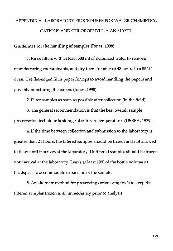
APPENDIX A. LABORATORY PROCEDURES FOR WATER CHEMISTRY,
CATIONS AND CHLOROPHYLL-A ANALYSIS.
Guidelines for the handling of samples (Jones, 1998):
1. Rinse filters with at least 500 ml of deionized water to remove
manufacturing contaminants, and dry them for at least 48 hours in a 55° C
oven. Use flat-edged filter paper forceps to avoid handling the papers and
possibly puncturing the papers Gones, 1998).
2. Filter samples as soon as possible after collection (in the field).
3. The general recommendation is that the best overall sample
preservation technique is storage at sub-zero temperatures (USEPA, 1979).
4. If the time between collection and submission to the laboratory is
greater than 24 hours, the filtered samples should be frozen and not allowed
to thaw until it arrives at the laboratory. Unfiltered samples should be frozen
until arrival at the laboratory. Leave at least 10% of the bottle volume as
headspace to accommodate expansion of the sample.
5. An alternate method for preserving cation samples is to keep the
filtered samples frozen until immediately prior to analysis.
179
\
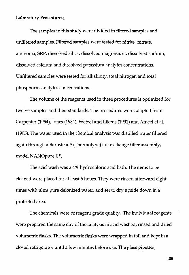
Laboratory Procedures:
The samples in this study were divided in filtered samples and
unfiltered samples. Filtered samples were tested for nitrite+nitrate,
ammonia, SRP, dissolved silica, dissolved magnesium, dissolved sodium,
dissolved calcium and dissolved potassium analytes concentrations.
Unfiltered samples were tested for alkalinity, total nitrogen and total
phosphorus analytes concentrations.
The volume of the reagents used in these procedures is optimized for
twelve samples and their standards. The procedures were adapted from
Carpenter (1994), Jones (1984), Wetzel and Likens (1991) and Ameel et al.
(1993). The water used in the chemical analysis was distilled water filtered
again through a Barnstead® (Thermolyne) ion exchange filter assembly,
model NANOpure II®.
The acid wash was a 4 % hydrochloric acid bath. The items to be
cleaned were placed for at least 6 hours. They were rinsed afterward eight
times with ultra pure deionized water, and set to dry upside down in a
protected area.
The chemicals were of reagent grade quality. The individual reagents
were prepared the same day of the analysis in acid washed, rinsed and dried
volumetric flasks. The volumetric flasks were wrapped in foil and kept in a
closed refrigerator until a few minutes before use. The glass pipettes,
180

borosilicate vials and its caps, the reusable tips of micropipettes, and the
stirrer bars were also acid washed, rinsed and dried.
The chlorophyll-a analysis was performed with a Turner Designs
Fluorometer Model 10-005R (No.5564) calibrated for chlorophyll. A Milton
Roy Spectronic® 401 spectrophotometer, with a wavelength range of 325 to
900 nanometers (nm) and equipped with a cell of 5 cm in length, was used
for the nutrient analysis. Concentrations were determined from the plot of
the absorbances of the standards versus their known concentrations (Wetzel
and Likens, 1991).
The cations analysis was performed with an AAnalyzer300®
manufactured by the Perkin-Elmer Corporation, and utilizing the flame
atomic adsorption technique. For the cations analysis, one blank and three
standards were always used.
For the titrations and other tasks in the laboratory that required pH
readings, an Orion® portable pH/Temperature/ m V 290A meter was used.
This meter was equipped with an Orion triode® electrode, with automatic
temperature compensation. The shaker machine was a Lab-Line Orbit Shaker
3590 from Lab-Line Instruments Inc.
181

Total Nitrogen:
Total nitrogen concentrations were determined after an alkaline
potassium persulfate digestion (Carpenter, 1994); (Ameel et al., 1993) and
followed by the cadmium reduction method (Jones, 1984).
Reagents:
A. -- Dissolve 0.722 grams of KN03 (previously oven dried at 105° C. for 24
hours) in 500 ml of ultra pure deionized water and then dilute this to 1 liter
using ultra pure deionized water, to produce a 100,000 µg. N/L stock
solution. Make a working solution of 1,000 µg. N/L by diluting the stock by
a ratio of 1:100; from this make six different standard solutions with
concentrations ranging from 2 to 200 µg N/L. Make an independent control
blank.
B. -- Dissolve 20 grams of potassium persulfate in 250 ml of ultra pure
deionized water and then dilute this to 500 ml using ultra pure deionized
water to obtain a solution with a concentration of 0.148 M
C. -- Dissolve 12 grams of NaOH in 75 ml of ultra pure deionized water and
then dilute this to 100 ml using ultra pure deionized water to obtain a 3 N
concentration. Let it cool before using.
182
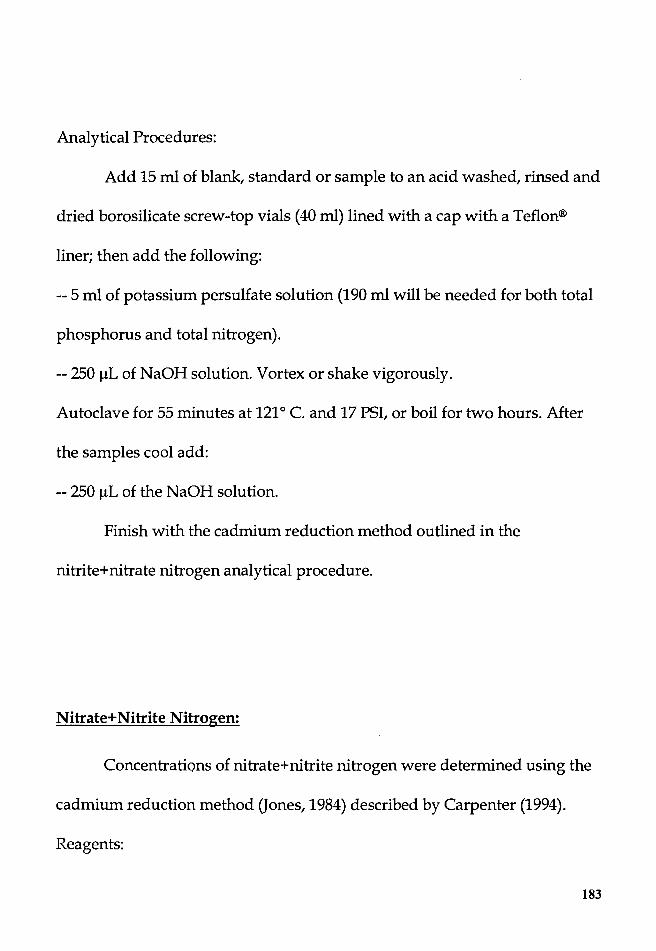
Analytical Procedures:
Add 15 ml of blank, standard or sample to an acid washed, rinsed and
dried borosilicate screw-top vials (40 ml) lined with a cap with a Teflon®
liner; then add the following:
-- 5 ml of potassium persulfate solution (190 ml will be needed for both total
phosphorus and total nitrogen).
--250 µL of NaOH solution. Vortex or shake vigorously.
Autoclave for 55 minutes at 121° C. and 17 PSI, or boil for two hours. After
the samples cool add:
-- 250 µL of the NaOH solution.
Finish with the cadmium reduction method outlined in the
nitrite+nitrate nitrogen analytical procedure.
Nitrate+Nitrite Nitrogen:
Concentrations of nitrate+nitrite nitrogen were determined using the
cadmium reduction method Gones, 1984) described by Carpenter (1994).
Reagents:
183
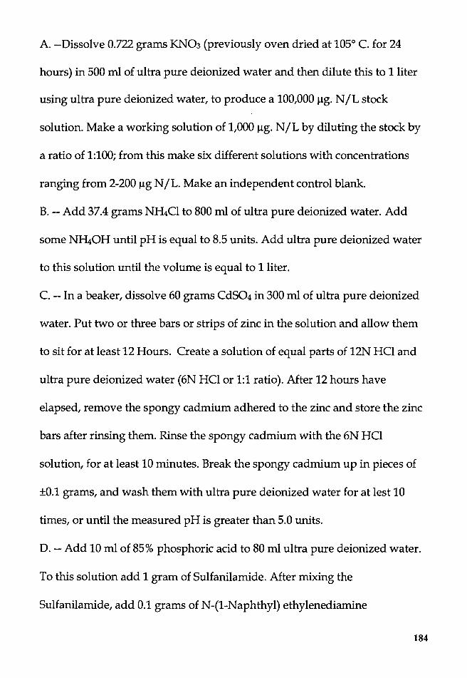
A. --Dissolve 0.722 grams KN03 (previously oven dried at 105° C. for 24
hours) in 500 ml of ultra pure deionized water and then dilute this to 1 liter
using ultra pure deionized water, to produce a 100,000 µg. N/L stock
solution. Make a working solution of 1,000 µg. N/L by diluting the stock by
a ratio of 1:100; from this make six different solutions with concentrations
ranging from 2-200 µg N/L. Make an independent control blank.
B. -- Add 37.4 grams NfuCl to 800 ml of ultra pure deionized water. Add
some NfuOH until pH is equal to 8.5 units. Add ultra pure deionized water
to this solution until the volume is equal to 1 liter.
C. - In a beaker, dissolve 60 grams CdS04 in 300 ml of ultra pure deionized
water. Put two or three bars or strips of zinc in the solution and allow them
to sit for at least 12 Hours. Create a solution of equal parts of 12N HCl and
ultra pure deionized water (6N HCl or 1:1 ratio). After 12 hours have
elapsed, remove the spongy cadmium adhered to the zinc and store the zinc
bars after rinsing them. Rinse the spongy cadmium with the 6N HCl
solution, for at least 10 minutes. Break the spongy cadmium up in pieces of
±0.1 grams, and wash them with ultra pure deionized water for at lest 10
times, or until the measured pH is greater than 5.0 units.
D. -- Add 10 ml of 85% phosphoric acid to 80 ml ultra pure deionized water.
To this solution add 1 gram of Sulfanilamide. After mixing the
Sulfanilamide, add 0.1 grams of N-(1-Naphthyl) ethylenediamine
184
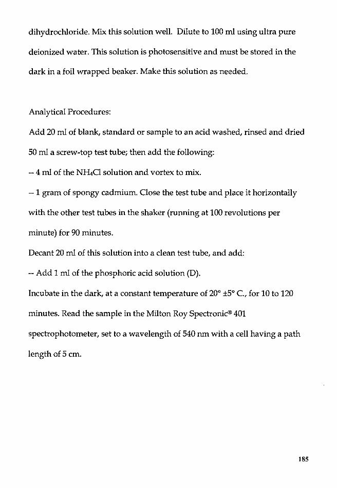
dihydrochloride. Mix this solution well. Dilute to 100 ml using ultra pure
deionized water. This solution is photosensitive and must be stored in the
dark in a foil wrapped beaker. Make this solution as needed.
Analytical Procedures:
Add 20 ml of blank, standard or sample to an acid washed, rinsed and dried
50 ml a screw-top test tube; then add the following:
-- 4 ml of the NH!Cl solution and vortex to mix.
-- 1 gram of spongy cadmium. Close the test tube and place it horizontally
with the other test tubes in the shaker (running at 100 revolutions per
minute) for 90 minutes.
Decant 20 ml of this solution into a clean test tube, and add:
-- Add 1 ml of the phosphoric acid solution (D).
Incubate in the dark, at a constant temperature of 20° ±5° C., for 10to120
minutes. Read the sample in the Milton Roy Spectronic® 401
spectrophotometer, set to a wavelength of 540 nm with a cell having a path
length of 5 cm.
185

Ammonium Nitrogen:
Concentrations of ammonium nitrogen were determined using the
phenol-hyplochlorite method outlined in Wetzel and Likens (1991) and
described by Carpenter (1994).
Reagents:
A. --Dissolve 3.819 grams NfuCl (Oven Dried at 105° C for 24 Hours) in 500
ml of ultra pure deionized water and then dilute this to 1 liter using ultra
pure deionized water, to produce a solution of 1,000,000 µg Nfu-N/L.
Make a working solution of 5,000 µg. N/L by diluting the stock by a ratio of
1:200; from this make six different solutions with concentrations ranging
from 10-400 µg N/L. Make an independent control blank.
B. -- Dissolve 5 grams N<13P04 in 250 ml of ultra pure deionized water and
then dilute this to 1 liter using ultra pure deionized water.
C. -- Dissolve 25 grams of phenol in 40 ml of methanol. This solution can be
stored refrigerated for up to 6 months.
D. -- Dissolve 27 grams of NaOH in 100 ml of ultra pure deionized water. Let
this solution cool.
Solution 1. -- Dissolve 0.01 grams of sodium nitroprusside in 7.5 ml of the
phenol solution (C). Add ultra pure deionized water to this solution until the
volume is equal to 50 ml This solution is photosensitive and must be stored
in the dark, in a foil wrapped beaker.
186
Solution 2. -- To 15 ml of NaOH solution (D) add 15 ml of sodium
hypochloride (or chlorine bleach of 5% chlorine). Add ultra pure deionized
water to this solution until the volume equals to 50 ml This solution is
photosensitive and must be stored in the dark in a foil wrapped beaker.
Analytical Procedures:
Add 25 ml of blank, standard or sample to an acid washed, rinsed and dried
50 ml a screw-top test tube; then add the following:
-- Add 1 ml of the NagPQ4 solution and vortex to mix well.
--Add 2.5 ml of the solution 1 (phenol+ sodium nitroprusside), and vortex
to mix well.
-- Add 1.5 ml of the solution 2 (NaOH and Chlorine), and vortex to mix well.
Incubate in the dark, at a constant temperature for 1 to 24 hours. Read the
sample in the Milton Roy Spectronic® 401 spectrophotometer, set to a
wavelength of 630 nm with a cell having a path length of 5 cm.
Total Phosphorus:
Concentrations of total phosphorus were determined after the alkaline
potassium persulfate digestion outlined by Ameel et. al. (1993) followed by
the ascorbic acid method (Wetzel and Likens 1991); Carpenter (1994).
Reagents:
187
A. -- Dissolve 0.2197 grams KH2P04 (Oven Dried at 105° C for 24 Hours) plus
1 ml of chloroform in 500 ml of ultra pure deionized water and then dilute
this to 1 liter using ultra pure deionized water, to produce a solution of
50,000 µg P /L. Make a working solution of 500 µg. P /L by diluting the stock
by a ratio of 1:100, from this make six different solutions with concentrations
ranging from 1-100 µg P /L. Make an independent control blank.
B. -- Dissolve 20 grams of potassium persulfate in 250 ml of ultra pure
deionized water and then dilute this to 500 ml using ultra pure deionized
water to obtain a solution with a concentration of 0.148 M
C. -- Dissolve 12 grams of NaOH in ultra pure deionized water and dilute
this to 100 ml using ultra pure deionized water to obtain a 3 N concentration.
Let it cool before using.
Analytical Procedures:
Add 15 ml of blank, standard or sample to an acid washed, rinsed and dried
borosilicate screw-top vials (40 ml) lined with a Teflon liner; then add the
following:
-- 5 ml of potassium persulfate solution.
-- 250 µL of NaOH solution. Vortex or shake vigorously.
Autoclave for 55 minutes at 121° C. and 17 PSI, or boil for two hours. After
the samples cool add:
188

-- 250 µL of the NaOH solution.
If necessary, refrigerate samples for up to 28 days. Finish analysis with the
ascorbic acid method outlined in the soluble reactive phosphorus analytical
procedure.
Soluble Reactive Phosphorus:
Concentrations of SRP were determined using the ascorbic acid
method described in Wetzel and Likens (1991) and modified by Carpenter
(1994).
Reagents:
A. -- Dissolve 0.2197 grams KH2P04 (Oven Dried at 105° C for 24 Hours) plus
1 ml of chloroform in 500 ml of ultra pure deionized water and then dilute
this to 1 liter using ultra pure deionized water, to produce a solution of
50,000 µg P /L. Make a working solution of 500 µg. P /L by diluting the stock
by a ratio of 1:100, from this make six different solutions with concentrations
ranging from 1-100 µg P /L. Make an independent control blank.
B. -- Dissolve 15 grams of ammonium (paramolybdate) molybdate in 250 ml
of ultra pure deionized water and then dilute this to 500 ml using ultra pure
deionized water. Store in the dark. The shelf life of this solution is of 2-3
months.
189
C. -- Dilute 135 ml of H2S04to1 liter using ultra pure deionized water. Store
in a stoppered glass bottle.
D. -- Dissolve 0.34 grams of potassium antimonyl-tartrate in 100 ml of ultra
pure deionized water and then dilute this to 250 ml using ultra pure
deionized water. Warm this solution if necessary, and store in a stoppered
glass bottle.
E. -- Dilute 2.7 grams of L-ascorbic acid to 50 ml using ultra pure deionized
water.
Composite solution: Make this solution just before using it. This composite
solution is photosensitive. Accordingly, it is kept in the dark, in an
Erlenmeyer flask with its mouth covered with parafilm. Mix this composite
in the following order.
-- Add 50 ml of the H2S04 solution.
-- Add 10 ml of the potassium antimonyl-tartrate solution.
-- Add 20 ml of the ammonium (paramolybdate) molybdate solution.
-- Add 20 ml of the L-ascorbic acid solution.
Analytical Procedures:
Add 20 ml of blank, standard or sample to an acid washed, rinsed and dried
50 ml a screw-top test tube; then add the following:
190
-- Add 2 ml of the composite solution, and vortex or shake well.
Incubate in the dark, at a constant temperature for 10 to 120 minutes.
Read the sample in the Milton Roy Spectronic® 401 spectrophotometer, set to
a wavelength of 880 nm with a cell having a path length of 5 cm.
Dissolved Silica
The concentrations of silica were determined using the method
described in Wetzel and Likens (1991) and by Carpenter (1994). If the silica
analysis is made on thawed samples, then these samples should be allowed
to stand for a period of time (1-7 days) to allow the silica to become reactive
again (Wetzel and Likens, 1991).
Reagents:
A. -- Dissolve 1.765 grams of sodium silica pentahydrate (previously
stabilized by placing in a dissector, for at least 3 hours) in 1 liter of ultra pure
deionized water. Dilute 100 ml of stock in 1 liter of ultra pure deionized
water to produce a working solution of 50 mg/L of Si02; from this make six
different solutions with concentrations ranging from 2.5 to 20 mg/L of Si02.
Make an independent control blank.
B. -- Dilute 22 ml of HCl to 1 liter (1000 ml) using ultra pure deionized water.
This will create a solution of a concentration of 0.25 N HCI.
191
C. -- Dissolve 52 grams of ammonium molybdate in (Nfu)6 Mo702 4H20) in
250 ml of ultra pure deionized water and then dilute this to 1 liter.
D. -- Dissolve 10 grams of EDTA in 250 ml of ultra pure deionized water and
dilute to 1 liter.
E. -- Dissolve 170 grams of sodium sulfate in 500 ml of ultra pure deionized
water and dilute to 1 liter.
Analytical Procedures:
Add 10 ml of blank, standard or sample to an acid washed, rinsed and dried
50 ml a screw-top test tube; then add the following:
-- 5 ml of the HCl solution, and vortex to mix well.
-- 5 ml of the ammonium molybdate solution and vortex to mix well. The
remaining reagents must be added five minutes of adding the ammonium
molybdate solution.
-- 5 ml of the EDTA solution, vortex to mix well.
-- 10 ml of the sodium sulfate solution, vortex to mix well.
Incubate in the dark, at a constant temperature for at least 30 minutes. Read
the sample in the Milton Roy Spectronic® 401 spectrophotometer, set to a
wavelength of 700 nm with a cell having a path length of 5 cm.
192
Major Cations: Mg, Na, Ca and K
The concentrations of major cations were determined from filtered
and pre-acidified samples using (flame) atomic absorption methods. The
procedures followed were those recommended by the manufacturer of the
instrument (Perkin-Elmer AAnalyst-300 spectrometer) and Beaty and Kerber
(1993). The handling of the sample followed the recommendations of Jones,
(1994).
Reagents:
A. -- The calcium, sodium, potassium and magnesium standards used in this
study came from commercial stock solutions (Sigma corporation). Make
three different solutions with concentrations ranging from 0.5-10 mg
Cation/L. Make an independent control blank Standards can be made in
the laboratory as follows:
K standard: stock standard: 1000 mg/L
Dissolve 1.907 grams of KCl in 250 ml of ultra pure deionized water
and then dilute this to 1 liter. For interferences add 0.1 % or more Cs or La to
samples (Perkin-Elmer, 1993).
Mg standard: stock standard: 100,000 µg/L
Dissolve 0.1658 gram of MgO in 50 ml of ultra pure deionized water,
add 10 ml of concentrated HN03, and then dilute this to 1 liter. (APHA,
1998).
193

Na standard: stock standard: 1000 mg/L
Dissolve 2.542 grams of NaCl in 50 ml of ultra pure deionized water
and then dilute this to 1 liter. For interferences add 0.1 % or more Kor Cs to
samples (Perkin-Elmer, 1993).
Ca standard: stock standard: 500 mg/L
Dissolve 1.249 grams of CaC03 in 50 ml of ultra pure deionized water.
Dissolve by adding the water drop-wise (slowly), add 10 ml of HCl, and then
dilute this to 1 liter. For interferences add alkali salt (0.1 % or more of K as
KCl) to samples (Perkin-Elmer, 1993).
Chlorophyll-a
The phaeophytin-corrected chlorophyll-a analysis followed the
procedure outlined in Daggett (1994), Axler and Owen (1994) and Honea
(1997).
Collect water sample in a dark bottle and filter in the dark within two
hours of collection. Use a glass microfiber filter (Whatman® GF /F 47 mm)
with a nominal pore size of 0.45 um. Wash filters with deionized water, and
oven-dry at 55° C. for at least 48 hours. To filter use a Nalgene® hand pump
filtration set up or a similar filtration set-up. After filtering add three drops
of saturated MgC03 to the filter. Place the filter in a filter holder, wrap in foil
194

and place it in ice and freeze until analysis. Before start of analysis create
standards to calibrate the instrument (Wetzel and Likens, 1991).
Materials:
Chlorophyll-a standards.
95% methanol (spectrophotometric grade).
0.12N HCl (1part36.5-38% HCl to 99 parts deionized water).
20 ml of saturated MgC03 solution.
Two 15 ml fluorometry cuvettes with caps per sample.
One 15 ml fluorometry cuvettes with caps per standard.
Pipettes (10 to 200 ml).
Turner Designs Fluorometer Model 10-005R (No.5564) calibrated for
chlorophyll. Turn on the fluorometer 30 minutes before use.
Procedures:
Label the fluorometric cuvettes. Cut up the filters with the samples using
tweezers, and place them in the 15 ml fluorometry cuvettes. Add 10 ml of
95 % methanol. Cap the cuvettes and shake it. Put cuvette rack in refrigerator
for 6-8 hrs (4° C).
Remove rack from refrigerator and invert tubes a couple times. If there is too
much debris or cloudiness in suspension, filter or centrifuge the sample.
Decant extract or pour the filtrate into clean cuvettes.
195
Read samples on fluorometer at room temperature and record
fluorometer setting (settings 1-4, 1 being the lowest).
Acidify with 200 ml 0.12 N HCl and invert it 4-5 times to mix. Immediately
neutralize with 4 drops saturated MgC03 solution. Invert 4-5 times to mix.
Read on fluorometer at same setting as pre-acidified sample. Use
equations listed here (Wetzel and Likens, 1991) to calculate chlorophyll-a
concentration corrected for Phaeophytin.
Using the chlorophyll-a standards, and for each setting, calculate the
values of 't and F. Where 't =Rb/Ra (Rb is the reading before acidification, and
Ra is the reading after acidification) and F = chl-a standard
concentration/ scale reading.
To calculate the chlorophyll-a concentration using (Wetzel and Likens, 1991):
Chlorophyll-a (µg/l) =
{(F)[('t/ ('t-1))] (Rb-Ra)} ·(vol. of extract/vol. of sample filtered)
Phaeopigment (µg/l) =
{(F)[('t/ ('t-1))] ('t (Ra -Rb)} (vol. of extract/vol. of sample filtered)
Finally, pour methanol waste into receptacle, and take to the
chemistry waste lab when the receptacle is full.
196
APPENDIX B. PLANKTON COUNTING METHODS.
Phytoplankton counting methods
Water samples for phytoplankton analysis were collected with the
Van Dorn bottle. To reach a 1 % final concentration of Lugol's fixative, 2.5 ml
of Lugol's solution was added to the 250 ml HDPE bottles marked for the
phytoplankton samples. Once in the laboratory, this sample was stored in
the dark, in a refrigerated room.
A modified sedimentation procedure was implemented to count the
phytoplankton. Dominant organisms were identified to species, and the rest
to genus. A minimum of 400-500 cells was counted from each sample.
Phytoplankton samples were placed on 250 ml beaker, 10 cm tall, and
allowed to settle for at least 5 days (1.2 hours/ ml). Supernatant was decanted
(±200 ml) and the remaining 50 ml were placed on a test tube. This test tube
was placed on a centrifuge (3000 rpm for 10 minutes) and the supernatant
was decanted again until only 20 ml remained. Samples from this
concentrate were placed on a Nannoplankton® counting chamber
(PhycoTech, Inc., Minnesota).
The Nannoplankton® counting chamber is a modified Palmer
Maloney counting cell. Most dominant organisms were identified to species,
197
and most others to genus. At least 500 cells were counted using a Nikon
Eclipse 600 microscope (magnifications of lOOx and 400x). The cells/ml
counts were transformed to µm/ ml.
Zooplankton counting methods
The zooplankton samples were collected using a folding plankton net
having a diameter of 49.5 cm, and a pore-mesh size of 130 µm. The filtration
efficiency of the net was 100%. The efficiency calculation was based on the
following formula: volume of water filtered/ (Area of the mouth of the net
times the distance or depth sampled (Wetzel and Likens, 1991).
Based on the temperature profile, and if a thermocline was present,
the vertical ranges for sampling were decided as follows: The epilimnion
sample covered the range from the surface of the reservoir to the beginning
of the metalimnion. The composite hypolimnion-metalimnion sample
covered the range from 1 m above the bottom of the reservoir to the
boundary between the metalimnion and the epilimnion. These ranges varied
in depth according to the water levels. During part of the fall 1998, the winter
1999 and part of the spring of 1999, when there was no stratification, the
range covered the entire water column.
198

The zooplankton was concentrated in the built-in collector bottle that
had a window covered with a fine mesh (48 µm). From the collector the
sample was transferred to the HDPE bottle marked for the zooplankton
samples. These bottles had been acid washed in the lab, and rinsed with
water from the reservoir. Depending on the amount of water in the sample,
from 1to3 ml of buffered formalin (40% formaldehyde) was added to
preserve the organisms; the aim was to achieve a final concentration of 4%.
Once in the laboratory, this sample was stored in the dark, in a refrigerated
room.
Zooplankton samples were mixed by shaking, and 50 ml were placed
on a test tube. This test tube was placed on a centrifuge (3000 rpm for 10
minutes) and the supernatant was decanted again until only 20 ml remained.
Samples from this concentrate were placed on a Sedgwick-Rafter counting
cell. Most dominant organisms were identified to species, and most others to
genus. At least 400 individuals were counted using a Nikon Eclipse 600
microscope (magnifications of lOOx and 400x). The individuals per ml counts
were transformed to µm per ml.
199