The Dynamics of Perception and Action - IGERT

The Dynamics of Perception and Action

William H. WarrenBrown University

How might one account for the organization in behavior without attributing it to an internal controlstructure? The present article develops a theoretical framework called behavioral dynamics that inte-grates an information-based approach to perception with a dynamical systems approach to action. For agiven task, the agent and its environment are treated as a pair of dynamical systems that are coupledmechanically and informationally. Their interactions give rise to the behavioral dynamics, a vector fieldwith attractors that correspond to stable task solutions, repellers that correspond to avoided states, andbifurcations that correspond to behavioral transitions. The framework is used to develop theories ofseveral tasks in which a human agent interacts with the physical environment, including bouncing a ballon a racquet, balancing an object, braking a vehicle, and guiding locomotion. Stable, adaptive behavioremerges from the dynamics of the interaction between a structured environment and an agent with simplecontrol laws, under physical and informational constraints.

Keywords: perception and action, perceptual–motor control, dynamical systems, self-organization,locomotion

The organization of behavior has been a central concern ofpsychology for well over a century. How is it that humans andother animals can generate behavioral patterns that are tightlycoordinated with the environment, in the service of achieving aspecific goal? This ability to produce stable yet adaptive behaviorraises two constituent issues. On the one hand, it implicates thecoordination of action, such that the many neuromusculoskeletalcomponents of the body become temporarily organized into anordered pattern of movement. On the other, it implicates percep-tion, such that information about the world and the body enablesappropriate actions to be selected and adapted to environmentalconditions. At a basic level, the problem of the organization ofbehavior is thus synonymous with the problem of perception andaction. Moreover, an adequate theory of perceptually controlledaction would provide a platform for understanding more “cogni-tive” behavior such as extended action sequences, anticipatorybehavior oriented to remote goals, or predictive behavior that takesaccount of hidden environmental properties.

It seems natural to presume that observed organization in be-havior implies ipso facto the existence of a centralized control-ler—a pattern generator, action plan, or internal model that isresponsible for its organization and regulation. Such an assumptionhas been commonplace in psychology, cognitive science, neuro-science, and robotics. In each domain, organization in behavior hasbeen attributed to prior organization in the structure of the nervous

system (the neuroreductionist view), the structure of internal rep-resentations (the cognitivist view), or in the contingencies pre-sented by the environment (the behaviorist view). This is unsatis-fying because it merely displaces the original problem ofbehavioral organization to a preexisting internal or external struc-ture, begging the question of why that particular organizationobtains and how that specific structure originated.

The challenge of accounting for organized behavior withoutresorting to an a priori controller was articulated by Gibson (1979):

Locomotion and manipulation . . . are controlled not by the brain butby information. . . . Control lies in the animal–environment system. . . .The rules that govern behavior are not like laws enforced by anauthority or decisions made by a commander; behavior is regularwithout being regulated. The question is how this can be. (p. 225)

Although the quotation asserts Gibson’s belief that behavior isregular without being centrally controlled, the question of how thiscan be remains open. His suggestion is that, rather than beinglocalized in an internal (or external) structure, control is distributedover the agent–environment system. I interpret this statement toimply that biology capitalizes on the regularities of the entiresystem as a means of ordering behavior. Specifically, the structureand physics of the environment, the biomechanics of the body,perceptual information about the state of the agent–environmentsystem, and the demands of the task all serve to constrain thebehavioral outcome. Adaptive behavior, rather than being imposedby a preexisting structure, emerges from this confluence of con-straints under the boundary condition of a particular task or goal.In the present article, I attempt to synthesize recent ideas to showhow the organization of behavior can be attributed to the dynamicsof the agent–environment interaction under such constraints andseek to develop a coherent theoretical framework for understand-ing perception and action.

Human and animal behavior exhibits two complementary at-tributes that need to be accounted for: stability and flexibility. On

Preparation of this article was supported by the National Eye Institute(Grant EY10923) and the National Institute of Mental Health (Grant K02MH01353). I thank Benoit Bardy and the University of Paris XI for theirgenerosity during preparation of the manuscript, and Elliot Saltzman andPeter Beek for their comments on an earlier draft.

Correspondence concerning this article should be addressed to WilliamH. Warren, Department of Cognitive and Linguistic Sciences, BrownUniversity, Providence, RI 02912. E-mail: [email protected]

Psychological Review Copyright 2006 by the American Psychological Association2006, Vol. 113, No. 2, 358–389 0033-295X/06/$12.00 DOI: 10.1037/0033-295X.113.2.358

358

the one hand, behavior is characterized by stable and reproduciblelow-dimensional patterns.1 These patterns are stable in the sensethat the functional form of movement is consistent over time andresists perturbation and reproducible in that a similar pattern mayrecur on separate occasions. On the other hand, behavior is notstereotyped and rigid but flexible and adaptive. Although actionpatterns exhibit regular morphologies, the agent is not locked intoto a rigidly stable solution but can modulate the behavioral pattern.To the extent that such flexibility is tailored to current environ-mental conditions or task demands, it implicates perceptualcontrol.

Let me state the proposal intuitively at the outset. Adaptivebehavior can be characterized on (at least) two levels of analysis.At the level of perception and action, the agent and the environ-ment can be treated as a pair of mutually coupled dynamicalsystems.2 They are coupled mechanically, through forces exertedby the agent, and informationally, through sensory fields that arestructured by the environment (optic, acoustic, haptic, olfactory,etc.). Agent–environment interactions give rise to emergent be-havior that has a dynamics of its own, which I call the behavioraldynamics. At this second level of analysis, the time evolution ofbehavior can be formally described by a dynamical system, whichmay represented as a vector field. The core claim is that stablebehavioral solutions correspond to attractors in the behavioraldynamics, and transitions between behavioral patterns correspondto bifurcations. Such stabilities do not inhere a priori in thestructure of the environment or in the structure of the agent but arecodetermined by the confluence of task constraints andperceptual–motor control laws. It is in this sense that, as Gibson(1979) proposed, control lies in the agent–environment system.

One consequence of this account is that behavior can be under-stood as self-organized, in contrast to organization being imposedfrom within or without. Behavior patterns emerge in the course oflearning, development, and even evolution through a bootstrappingprocess in which agent–environment interactions give rise to thebehavioral dynamics, and stabilities in these dynamics in turn actto capture the behavior of the agent. During bootstrapping, theagent actively explores the vector field for a task, both contributingto and locating its stabilities; to express this combination of cre-ation and discovery, one might say that stable solutions are enactedby the agent (Varela, Thompson, & Rosch, 1991). Reciprocally,attractors in the behavioral dynamics feed back to fix the agent’saction patterns and control laws, in a form of circular causality.Thus, rather than a central controller dictating the intended behav-ior, the agent develops perceptual–motor mappings that tweak thedynamics of the system in which it is embedded so that the desiredbehavior arises from the entire ensemble. From the agent’s point ofview, the task is to exploit physical and informational constraintsto stabilize the intended behavior. As shown below, the solutionmay rely more or less upon physical or informational regularities,depending on the nature of the task. Consequently, behavior is notprescribed by internal or external structures, yet within the givenconstraints there are typically a limited number of stable solutionsthat achieve the desired outcome.

The study of adaptive behavior can, of course, be extended tomore micro (e.g., neuromuscular) levels of analysis but at the priceof introducing a higher dimensional and hence less tractable de-scription. The approach taken here is to adopt a scale of description

that is commensurate with the scale of observed regularity. Sys-tematicity in goal-directed behavior is manifested in low-dimensional action patterns directed at medium-scale features ofthe environment and guided by higher order informational vari-ables, whereas at the level of neuromuscular degrees of freedom,such behavior exhibits considerable contextual variation. Althoughit is important to study the correlates between the neural supportfor action and observed behavioral patterns, I would argue that thisrelationship is complementary rather than reductive. A theoreticalaccount of behavior must incorporate goals, information, physics,and properties of the world that are not directly reducible to aneural level (Koenderink, 1999). Thus, the aim of this article is toseek a lawful account of behavior at a functional level.

Background

Explaining behavioral organization by postulating an antecedentinternal representation that specifies the movement pattern has along history in theories of motor control and has also been influ-ential in recent theories of perception and action. In this section, Icursorily review the major modern approaches, including the re-cent disenchantment with a representational view.

Model-Based Approaches

Beginning in the 1960s and 1970s, the motor programmingapproach attributed movement patterns to motor plans that speci-fied a sequence of muscle commands (Keele, 1968) or to moreabstract motor schemata that specified the form of a class ofmovements, with the details filled in through a hierarchical controlscheme (Greene, 1972; R. A. Schmidt, 1975). Environmental andbiomechanical constraints played little role in the formulation ofsuch programs, and perception was simply assumed to deliver therequired input, such as the coordinates of a target. This approachessentially redescribed the organization of action in the form of atime-independent internal representation, without resolving thequestion of how that representation was arrived at to begin with. Arelated problem was that motor programs tended to ignore thetime-dependent kinematics and dynamics of the peripheral mus-culoskeletal system involved in the execution of movement (Bern-stein, 1967), one that became apparent with the advent of roboticcontrol. Specifically, because the relation between a motor com-mand or muscle activation and the resulting movement is nonlinearand context dependent, the motor system must somehow determinethe command that is required to achieve a desired outcome.

To address this problem, work in computational motor controlincreased the demands on representation, introducing internalmodels of the controlled system or “plant” (M. I. Jordan & Wol-pert, 1999; Kawato, 1999). First, inverse models of the dynamics

1 One indication of their low dimensionality is that principal-components analysis of the kinematics of whole-body movements withmany degrees of freedom reveals that the variability can be largely ac-counted for by the first several modes (Daffertshofer, Lamoth, Meijer, &Beek, 2004; Hollands, Wing, & Daffertshofer, 2004).

2 Exactly where lines between agent and environment are drawn islargely a matter of convenience, because in the end this analysis applies tothe coupled system.

359DYNAMICS OF PERCEPTION AND ACTION

of the musculoskeletal system were proposed to compute thecommand that, given the current state of the system, will producethe desired movement (Kawato, Furawaka, & Suzuki, 1987; Shad-mehr & Mussa-Ivaldi, 1994). More recently, forward models of themusculoskeletal system have been proposed to compensate forsensory delays by rapidly predicting the movement outcome, giventhe current state of the system and an efference copy of the motorcommand (Wolpert, Ghahramani, & Jordan, 1995). As M. I. Jor-dan and Wolpert (1999) put it, the controller in effect controls theinternal model, not the physical body. Finally, because both typesof models depend on knowing the current state of the musculo-skeletal system, a process of state estimation based on a Kalmanfilter has also been proposed (Wolpert et al., 1995).

This control engineering approach is committed to particularmechanisms at Marr’s (1982) algorithmic level of description thatrepresent prior knowledge on the part of the nervous system aboutthe motor apparatus and its context, which must ultimately beaccounted for by the theory. To the extent that internal models canbe learned on the basis of motor practice alone (M. I. Jordan &Wolpert, 1999), they gain in plausibility. For example, forwardmodels might be learned by comparing the predicted movementoutcome for a given motor command with the actual outcome andusing the difference as an error signal. Inverse models, by contrast,are more difficult to learn because of nonlinearities in the input–output mapping and the absence of a “correct” motor command toserve as a teaching signal, although Kawato et al. (1987; Wolpert& Kawato, 1998) developed a feedback error learning scheme todo so. For the most part, motor theories have not addressedagent–environment interactions. One exception is the recent ex-tension of forward models to anticipate the weight of environmen-tal objects (Wolpert & Ghahramani, 2000). Whether these partic-ular architectures and assumptions offer an appropriate descriptionof biological systems remain an open question.

Recent work within an optimal control framework (Engelbrecht,2001; Todorov & Jordan, 2002) considers the problem at the levelof computational theory (Marr, 1982). Optimal control is a set oftechniques for determining the control signals for a system withgiven dynamics that will minimize an objective or cost functionwhile satisfying specified constraints (Kirk, 1970). In this ap-proach, movement trajectories are not explicitly planned but are aconsequence of the objective function and the system’s dynamics.Most work in this vein has focused on the nature of the objectivefunction, such as minimizing jerk, energy, motor variance, orperformance error (Flash & Hogan, 1985; C. M. Harris & Wolpert,1998). But Berthier, Rosenstein, and Barto (2005) pointed out thattaking full advantage of the natural dynamics of the task is oftenthe essence of the problem. Indeed, using a method such asreinforcement learning (Kaelbling, Littman, & Moore, 1996; Sut-ton & Barto, 1998) to acquire a sensor–effector mapping thatexploits the natural dynamics can yield stable movement patternswithout explicit internal models (Berthier et al., 2005; Collins,Ruina, Tedrake, & Wisse, 2005; Ng, Kim, Jordan, & Sastry, 2004).This points theorists toward a richer analysis of the natural dy-namics and other task constraints as a basis for understanding thestructure of behavior.

A reliance on internal models has recurred in theories of per-ception and action, which seek to account for adaptive behavior asan agent interacts with its environment. Consistent with this view,

the function of perception is commonly taken to be the construc-tion of an internal 3-D representation of the environment frominadequate sensory data (Knill & Richards, 1996; Marr, 1982).This representation is thought to be sufficiently rich and generalpurpose to provide the basis for any action, such that neither therelevant information nor the structure of the representation de-pends on the particular task. In robotics, for example, a standardcontrol architecture has used what Brooks (1995) called the“sense–model–plan–act” framework, in which sensor input is usedto construct a 3-D model of the immediate environment. Thisworld model provides the basis for computing an explicit actionplan, which is finally executed by the robot’s effector system.

An analogous model-based framework has recently been ap-plied to perception and action in biological systems. Loomis andBeall (2004) argued that the control of complex action requiresboth a perceptual representation of the surrounding environmentand an internal model of the plant dynamics—including the body,manipulated objects, controlled vehicles, and other aspects of thephysical world with which the agent interacts. The primary evi-dence for a perceptual representation is that “visually directed”actions, such as blind walking to a previously viewed target, can beperformed for a short time after vision is removed, implying apersisting representation of the spatial layout. However, suchoff-line behavior might also be supported by partial, task-specificknowledge of a few target locations rather than a world model(Ballard, Hayhoe, & Peltz, 1995), and in either case, it does notfollow that representations are invoked in ordinary online controlwhen occurrent information is available. In an interactive task suchas steering a slalom course, accurate performance actually dependson seeing the next upcoming target, and error increases dramati-cally if it goes out of sight (Duchon & Warren, 1997). Similarly,Loomis and Beall (2004) argued that an internal model of plantdynamics would be supported by successful control of a vehicleafter vision is removed, but current evidence shows that drivingperformance degrades sharply under these conditions (Hildreth,Beusmans, Boer, & Royden, 2000; Wallis, Chatziastros, &Bulthoff, 2002).

A middle path has been proposed in the form of the two visualsystems hypothesis (Milner & Goodale, 1995; Norman, 2002). Inthis view, online, visual–motor behavior is ascribed primarily tothe dorsal visual pathway, whereas off-line, model-based behavioris ascribed to the ventral visual pathway. However, positing neuralloci for these functions does not constitute a theory of either one,and an account of the informational and dynamical bases ofperception and action is still called for. Another sort of compro-mise might be to accept a role for inverse and forward models inlow-level motor control, for example to solve the inverse dynamicsproblem, without generalizing them to world and plant models inperception and action.

The model-based approach leads to a somewhat solipsistic viewof perception and action, in which the perceiver is not actually incontact with the environment but only an internal representationthereof (Fodor, 1980), and the actor does not actually control his orher own body but only an internal model thereof (M. I. Jordan &Wolpert, 1999). The fact that behavior is generally effective andadaptive is attributed to the functional fidelity of these represen-tations, which presumes they are grounded in the physical world.However, this reliance on internal representations in cognitive

360 WARREN

theory faces numerous conceptual and philosophical obstacles(Bickhard & Terveen, 1995; Searle, 1980; Shannon, 1993; Shaw,2003). For instance, one must account for the origin of represen-tational content without appealing in circular fashion to the veryperception and action abilities they purport to explain. If percep-tual states are representations, how is it possible for the agent toknow what they stand for without presuming some other directaccess to the world? Similarly, invoking representations in actionalso runs the risk of an explanatory regress, accounting for orga-nization in behavior by attributing it to prior organization in therepresentational realm. Such considerations have led other re-searchers to seek an account of behavior that minimizes the role ofinternal representations.

Non-representational Approaches

The dynamical approach to human movement developed in the1980s and 1990s and has had a significant impact in the motorcontrol literature (Kelso, 1995; Kugler, Kelso, & Turvey, 1980;Kugler & Turvey, 1987; Saltzman & Kelso, 1987). This viewemphasizes physical principles and concepts from nonlinear dy-namics to explain interlimb coordination as a natural process ofpattern formation. One strength of the approach is its promotion ofdynamics as a common theoretical language for describing theworld, the body, and the neural and sensory couplings involved incoordination.

In his seminal research on coordination, Kelso and his col-leagues (Haken, Kelso, & Bunz, 1985; Kelso, Scholz, & Schoner,1986; Scholz, Kelso, & Schoner, 1987) found that two oscillatinglimbs are stably entrained at phase relations of 0° and 180° andundergo a spontaneous phase transition from an antiphase to anin-phase pattern as the frequency of movement is increased. Bor-rowing from the analysis of physical systems (Haken, 1977), Kelsoand colleagues refer to phase as an order parameter, because itindexes the order or organization of the movement, and refer tofrequency as a control parameter, because it induces a qualitativechange in phase at a critical value. Kelso and colleagues christenedthe formal analysis of such coordination phenomena coordinationdynamics.

The observation that similar coordination phenomena occurbetween perceptually coupled oscillators, such as a swarm ofMalaysian fireflies (Ermentrout & Rinzel, 1984), the limbs of twopeople (R. C. Schmidt, Carello, & Turvey, 1990), and even theperceived stability of two moving lights (Bingham, Zaal, Shull, &Collins, 2001), led Kelso to view coordination dynamics as fun-damentally informational rather than physical (Kelso, 1994, 1995;Schoner & Kelso, 1988a). Information can serve as a couplingmedium and can specify required coordinative relations (i.e., thedesired limb phasing) but must be expressed in the same dimen-sions as the order parameter itself (i.e., phase). This view ofinformational variables emphasizes their mirroring of coordinationdynamics rather than their specification of environmental condi-tions. The varied interactions an agent has with a complex envi-ronment call for a richer account of the information that guidesbehavior.

In addition, most research on coordination dynamics to date hasfocused on fairly simple tasks with stationary dynamics, such asrhythmic movement or interlimb coordination. For perception and

action in a complex world, the dynamics are often nonstationary,evolving as the interaction between agent and environment un-folds. The present article thus shifts emphasis from the dynamicsof movement coordination to the behavioral dynamics—the dy-namics of temporal and spatial coordination between an agent andits environment. Although this bears similarities to what Saltzmanand Kelso (1987) have called “task dynamics,” I use the termbehavioral dynamics to emphasize adaptive behavior by an agentin an environment, coupled by perceptual information.

Alongside the dynamical approach to movement there devel-oped the ecological perception–action approach to the control ofbehavior (Gibson, 1958/1998, 1979; Lee, 1976, 1980; Shaw, Ku-gler, & Kinsella-Shaw, 1990; Turvey & Carello, 1986; Warren,1988, 1998). This view emphasizes the role of occurrent informa-tion in guiding behavior, in the form of optic, acoustic, haptic, orolfactory fields that are structured by and are specific to the stateof the agent–environment system. The research program involvesdetermining what informational quantities govern naturalistic be-haviors like reaching, catching, hitting, standing posture, or loco-motion. Information is viewed as regulating action directly, in atask-specific manner, rather than contributing to a general-purposeworld model for the planning of action. The strength of thisinformation-based approach is its analysis of action-relevant in-formational variables, but it has yet to show how they can beintegrated with the dynamics of action (Beek & van Wieringen,1994). That is a central aim of the present article.

Related developments also transpired in artificial intelligence,with the questioning of model-based vision and model-based con-trol. The active vision approach (Bajcsy, 1988; Ballard, 1991)sought alternatives to the difficulty of computing a sufficientlydetailed general-purpose world model and instead advocated tak-ing advantage of task constraints to arrive at simple, special-purpose solutions for specific tasks. To steer a robot vehicle, forexample, several groups developed visual servoing systems thatexploited specific image features, such as the boundary corre-sponding to the edge of the road, to directly control the vehicle,rather than computing a 3-D reconstruction of the scene (Raviv &Herman, 1993). As Brooks (1991a) put it, the world is its own bestmodel, and sensor systems can obtain information as needed forthe task at hand. This point has been echoed in human vision byresults on change blindness (O’Regan, 1992; Rensink, O’Regan, &Clark, 1997) and gaze behavior in natural tasks (Ballard et al.,1995; Hayhoe, 2000), which suggest that perception is stronglydependent on the attended information and that any visual repre-sentation of the world is fragmentary and fleeting.

At the same time, researchers in behavior-based robotics(Brooks, 1986, 1991b) and the simulation of behavior (Beer, 1990;Meyer & Wilson, 1991) sought alternatives to model-based con-trol. Emphasizing that an agent is embodied in a physical platformand embedded in a physical world, they proposed exploiting suchconstraints to simplify the control architecture. In behavior-basedrobots, behavior emerges from the interaction between a structuredworld and an agent endowed with elementary behavioral routines,rather than being planned in advance on the basis of a worldmodel. However, such systems are purely reactive, and their be-havioral repertoire has been limited; they also tend to have ahierarchical control structure, thus preserving a discrete logic atopa continuous physics.


An instructive alternative has been developed by Schoner andhis colleagues (Schoner & Dose, 1992; Schoner, Dose, & Engels,1995), in which behavior is governed by a dynamical systemdefined over the state of the robot and the sensed state of theenvironment. Flexibility is obtained from nonlinearity by havingelementary behaviors compete with one another, rather than hav-ing a fixed dominance hierarchy. Thus, both agent and environ-ment contribute to control, and a common dynamical language isapplied at all levels of description. Similar ideas have been for-mulated by Shaw (Shaw, Kadar, Sim, & Repperger, 1992; Shaw etal., 1990, Beer (1995, 1997), and Smithers (1994). The presentframework for biological control is indebted to the approach ofSchoner and his colleagues.

My argument synthesizes four themes that run through thisspectrum of research: (a) Embodiment and embeddedness. Theagent possesses a physical body and is embedded in a physicalenvironment, which provide nontrivial sources of constraint onstable behavioral solutions. (b) Information-based control. Behav-ior is guided by occurrent information about the state of theagent–environment system. The available information providesanother important source of constraint on stable solutions. (c)Task-specificity. Control relations are task specific, mapping rel-evant informational quantities to relevant action variables. Thisallows the agent to adopt special-purpose solutions that makeminimal demands on internal representation, rather than general-purpose solutions that depend on elaborated world and plant mod-els. (d) Emergent, self-organized behavior. Behavior emerges fromthe interaction of the agent and the environment, under physical,informational, and task constraints. By emergent I mean a patternof behavior that does not reside a priori in the individual compo-nents of the system but is a consequence of their interdependenceand interaction (Bar-Yam, 2004; Corning, 2002). Reciprocally, thedynamics of this interaction feed back to capture the individualcomponents, serving to stabilize particular action patterns. In thisway, new forms of adaptive behavior are self-organized.

In what follows, my aim is to understand the stabilization ofadaptive, goal-directed behavior. First, some pertinent conceptsfrom nonlinear dynamics are introduced, prefatory to a formaldescription of the dynamics of perception and action. I then de-scribe a taxonomy of tasks based on physical and informationalstability and illustrate the framework by developing three exam-ples: ball bouncing, pole balancing, and braking. Finally, I putthese ideas to work in a theory of the behavioral dynamics ofhuman locomotion.

Dynamics

Before we can consider the dynamics of perception and action,some basic concepts must be introduced. (Readers already familiarwith these topics can skip to the next section.) The field ofnonlinear dynamics offers useful tools for analyzing and modelingpatterns of stability and change in a system’s behavior. In thepresent context, the dynamical hypothesis proposes that the mor-phology of human and animal behavior can be formalized in termsof low-dimensional dynamical systems (Kugler et al., 1980; Yates& Iberall, 1973). In particular, preferred stable modes of behaviorcan be identified with attractors, and qualitative transitions be-tween them with bifurcations in the system’s dynamics.

Dynamics is the study of change in a system over time (seeAcheson, 1997; D. W. Jordan & Smith, 1977; Strogatz, 1994). Oneway to represent change is in the form of a time series, which plotsthe value of a particular variable as an explicit function of time.Over time, for example, a variable might settle down to a stableequilibrium, blow up to infinity, repeat in a regular periodicpattern, exhibit irregular chaotic patterns, behave randomly, orswitch suddenly from one pattern to another. More generally, asystem can be described by a set of state variables (x1, x2,. . . xn),and its current state by a location in the state space defined bythose variables. The behavior of the system is thus characterizedby changes in the state variables and can be represented as atrajectory in state space, so that time is implicit.

The aim of analysis is to formalize this behavior as a dynamicalsystem, a system of first-order differential equations in which therate of change in each variable is a function of the current state ofthe system:

x1 � f1(x1, x2, . . . , xn)

x2 � f2(x1, x2, . . . , xn)

···xn � fn(x1, x2, . . . , xn). (1)

Exhibited behavior corresponds to solutions of these equations ofmotion for given initial conditions and can be represented astrajectories in state space. Loci in state space toward which tra-jectories converge from different initial conditions are known asattractors, and those from which trajectories diverge as repellers.Continuous change in system parameters can produce suddenchanges in the number or stability of attractors or repellers, whichare known as bifurcations. By formally expressing behavior in thisway, one can achieve a deeper understanding of the underlyingmorphology of stabilities and instabilities that govern observedbehavior.

Dynamical systems can be classified in terms of their dimen-sionality, the number of state variables minimally required topredict the future state of the system, and their linearity, whetherthe equations of motion contain nonlinear terms.3 A one-dimensional system has a single state variable x. For example,

x � �rx (2)

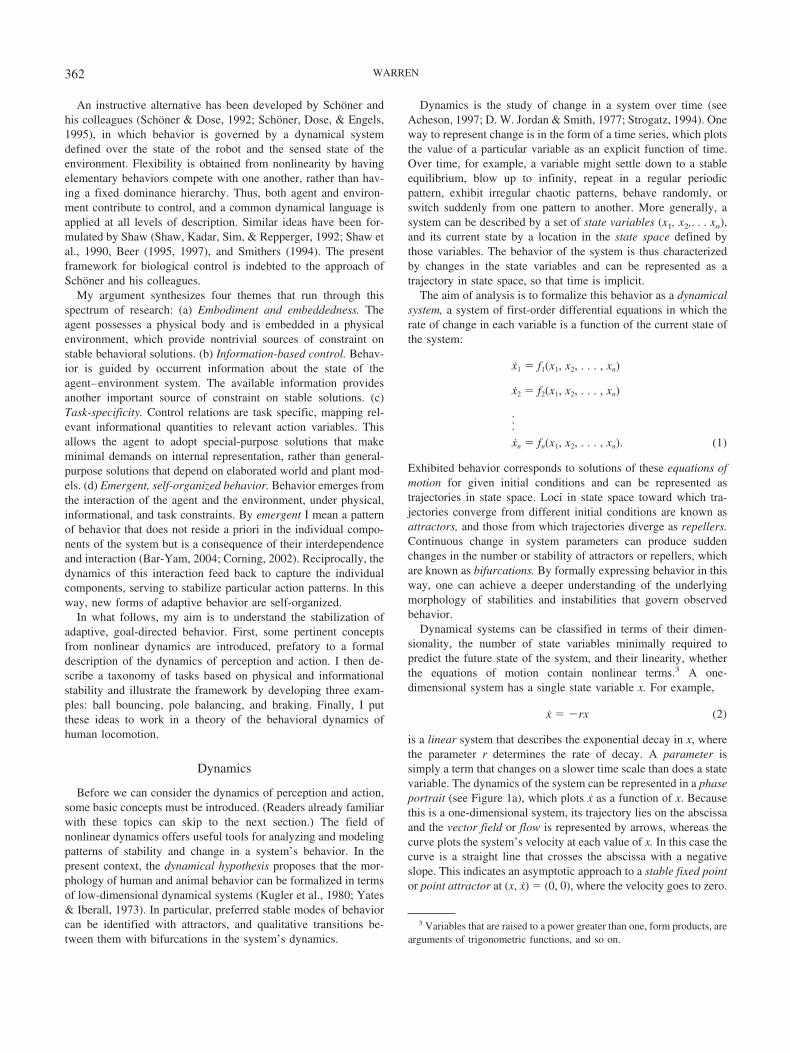
is a linear system that describes the exponential decay in x, wherethe parameter r determines the rate of decay. A parameter issimply a term that changes on a slower time scale than does a statevariable. The dynamics of the system can be represented in a phaseportrait (see Figure 1a), which plots x as a function of x. Becausethis is a one-dimensional system, its trajectory lies on the abscissaand the vector field or flow is represented by arrows, whereas thecurve plots the system’s velocity at each value of x. In this case thecurve is a straight line that crosses the abscissa with a negativeslope. This indicates an asymptotic approach to a stable fixed pointor point attractor at (x, x) � (0, 0), where the velocity goes to zero.

3 Variables that are raised to a power greater than one, form products, arearguments of trigonometric functions, and so on.

362 WARREN

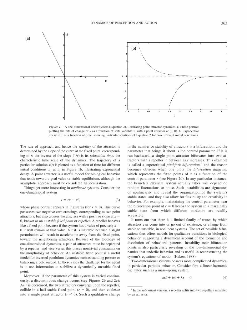
The rate of approach and hence the stability of the attractor isdetermined by the slope of the curve at the fixed point, correspond-ing to r; the inverse of the slope (1/r) is its relaxation time, thecharacteristic time scale of the dynamics. The trajectory of aparticular solution x(t) is plotted as a function of time for differentinitial conditions x0 at t0 in Figure 1b, illustrating exponentialdecay. A point attractor is a useful model for biological behaviorthat tends toward a goal value or stable equilibrium, although theasymptotic approach must be considered an idealization.

Things get more interesting in nonlinear systems. Consider theone-dimensional system

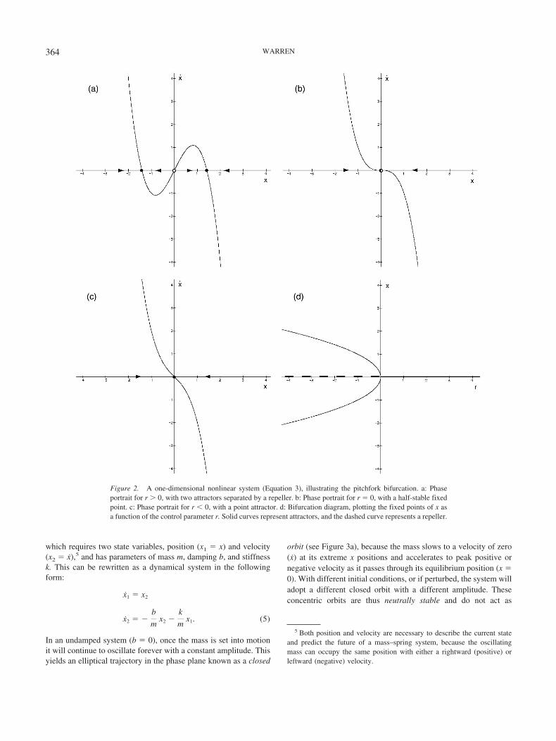
x � rx � x3, (3)

whose phase portrait appears in Figure 2a (for r � 0). This curvepossesses two negative zero crossings, corresponding to two pointattractors, but also crosses the abscissa with a positive slope at x �0, known as an unstable fixed point or repeller. A repeller behaveslike a fixed point because if the system has a value of precisely x �0 it will remain at that value, but it is unstable because a slightperturbation will result in acceleration away from the fixed point,toward the neighboring attractors. Because of the topology ofone-dimensional dynamics, a pair of attractors must be separatedby a repeller, and vice versa; this places nontrivial constraints onthe morphology of behavior. An unstable fixed point is a usefulmodel for inverted pendulum dynamics such as standing posture orbalancing a pole on end. In these cases the challenge for the agentis to use information to stabilize a dynamically unstable fixedpoint.

Moreover, if the parameter of this system is varied continu-ously, a discontinuous change occurs (see Figures 2b and 2c):As r is decreased, the two attractors converge upon the repeller,collide in a half-stable fixed point (r � 0), and then coalesceinto a single point attractor (r � 0). Such a qualitative change

in the number or stability of attractors is a bifurcation, and theparameter that brings it about is the control parameter. If it isrun backward, a single point attractor bifurcates into two at-tractors with a repeller in between as r increases. This exampleis called a supercritical pitchfork bifurcation,4 and the reasonbecomes obvious when one plots the bifurcation diagram,which represents the fixed points of x as a function of thecontrol parameter r (see Figure 2d). In any particular instance,the branch a physical system actually takes will depend onrandom fluctuations or noise. Such instabilities are signaturesof nonlinearity and reveal the organization of the system’sstable states, and they also allow for flexibility and creativity inbehavior. For example, maintaining the control parameter nearthe bifurcation point at r � 0 keeps the system in a marginallystable state from which different attractors are readilyaccessible.

It turns out that there is a limited family of routes by whichattractors can come into or go out of existence, or change fromstable to unstable, in nonlinear systems. The set of possible bifur-cations thus offers models for qualitative transitions in biologicalbehavior, suggesting a dynamical account of the formation anddissolution of behavioral patterns. Instability near bifurcationpoints is also particularly revealing of the low-dimensional dy-namics that underlie behavior and is useful in reconstructing thesystem’s equations of motion (Haken, 1988).

Two-dimensional systems possess more complicated dynamics,in particular periodic behavior. Consider first a linear harmonicoscillator such as a mass–spring system,

mx � bx � kx � 0, (4)

4 In the subcritical version, a repeller splits into two repellers separatedby an attractor.

Figure 1. A one-dimensional linear system (Equation 2), illustrating point-attractor dynamics. a: Phase portraitplotting the rate of change of x as a function of state variable x, with a point attractor at (0, 0). b: Exponentialdecay in x as a function of time, showing particular solutions of Equation 2 for two different initial conditions.


which requires two state variables, position (x1 � x) and velocity(x2 � x),5 and has parameters of mass m, damping b, and stiffnessk. This can be rewritten as a dynamical system in the followingform:

x1 � x2

x2 � �b

mx2 �

k

mx1. (5)

In an undamped system (b � 0), once the mass is set into motionit will continue to oscillate forever with a constant amplitude. Thisyields an elliptical trajectory in the phase plane known as a closed

orbit (see Figure 3a), because the mass slows to a velocity of zero(x) at its extreme x positions and accelerates to peak positive ornegative velocity as it passes through its equilibrium position (x �0). With different initial conditions, or if perturbed, the system willadopt a different closed orbit with a different amplitude. Theseconcentric orbits are thus neutrally stable and do not act as

5 Both position and velocity are necessary to describe the current stateand predict the future of a mass–spring system, because the oscillatingmass can occupy the same position with either a rightward (positive) orleftward (negative) velocity.

Figure 2. A one-dimensional nonlinear system (Equation 3), illustrating the pitchfork bifurcation. a: Phaseportrait for r � 0, with two attractors separated by a repeller. b: Phase portrait for r � 0, with a half-stable fixedpoint. c: Phase portrait for r � 0, with a point attractor. d: Bifurcation diagram, plotting the fixed points of x asa function of the control parameter r. Solid curves represent attractors, and the dashed curve represents a repeller.

364 WARREN

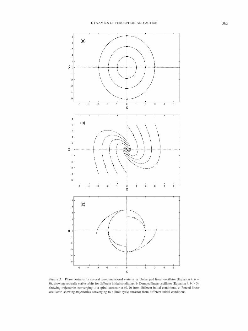
Figure 3. Phase portraits for several two-dimensional systems. a: Undamped linear oscillator (Equation 4, b �0), showing neutrally stable orbits for different initial conditions. b: Damped linear oscillator (Equation 4, b � 0),showing trajectories converging to a spiral attractor at (0, 0) from different initial conditions. c: Forced linearoscillator, showing trajectories converging to a limit cycle attractor from different initial conditions.


attractors. If damping is added (b � 0), the mass slows to rest atthe static equilibrium point in the center (x, x) � (0, 0), which isa stable focus or spiral attractor (see Figure 3b).

In nonlinear systems, closed orbits can form periodic attractorsknown as limit cycles. For example, suppose we force the har-monic oscillator,

mx � bx � kx � F(�), (6)

using an intrinsic forcing function that depends on the system’sown phase �, like a grandfather clock with an escapement. Thisrenders the oscillator nonlinear because the forcing function isperiodic and autonomous because it does not depend explicitly ontime. The system now displays self-sustained oscillation with astable frequency and amplitude. In the phase plane (see Figure 3c),the trajectories all spiral asymptotically toward a single closedorbit and return to it following a perturbation. Hence, the orbit isa stable limit-cycle attractor,6 and the point in the center is anunstable fixed point that repels the system toward the limit cycle.

Another autonomous limit cycle is the van der Pol oscillator,

x � b(x2 � 1)x � kx � 0. (7)

Rather than being externally forced, it has a nonlinear dampingterm that depends on the oscillator’s position. This acts like normalpositive damping when �x� � 1 but changes to negative dampingwhen �x� � 1. Thus, if the amplitude of oscillation is either toolarge or too small, it is returned to the limit cycle that passesthrough �x� � 1. Other examples include the Rayleigh oscillator,which has a nonlinear damping that depends on velocity, and theDuffing oscillator, which has a nonlinear stiffness. Periodic attrac-tors have an associated family of bifurcations as well. For exam-ple, the onset of oscillation is captured by the Hopf bifurcation. Inits subcritical version, a stable fixed point that is surrounded by alimit cycle suddenly becomes unstable, so the system jumps to thelimit cycle.

Such self-sustained periodic behavior is ubiquitous in biology,ranging from locomotor gaits and circadian rhythms to skills suchas hammering, dribbling, hopping on a pogo stick, or bouncing aball on a racquet. Coupled nonlinear oscillators can exhibit stableentrainment, in which their phases and frequencies become modelocked (D. W. Jordan & Smith, 1977). Local interactions betweenoscillatory components thus offer a natural basis for explainingtemporal coordination in biological systems (Haken et al., 1985;Kopell, 1988; Strogatz & Steward, 1993; von Holst, 1980).

Finally, three-dimensional nonlinear systems can exhibit com-plex, chaotic dynamics. For example, by extrinsically forcing anonlinear oscillator such as the Duffing, one can observe strangeattractors, chaotic oscillations that remain in a bounded region ofstate space but never settle down into a stable orbit. In this case theoscillator is nonautonomous because the forcing function dependsexplicitly on time, and hence the system has three state variables(x, x, t). Such chaotic systems may also undergo bifurcations. Forexample, the classic period-doubling route to chaos proceedsthrough a series of bifurcations to a chaotic regime, doubling thenumber of oscillations per cycle at each critical value of a controlparameter.

There is thus a limited bestiary of attractors and bifurcations outof which behavior can be assembled. This suggests the hypothesis

that the essential forms of all stable patterns of biological behaviorare composed of low-dimensional fixed points, limit cycles, orstrange attractors, with a restricted topology of layouts. Similarly,transitions between behavioral patterns should take the form of alimited set of bifurcations. Nonlinear dynamics thus provides apowerful theoretical language for characterizing the morphologyof behavior, in terms of which specific theoretical claims aboutparticular tasks can be formulated.

Behavioral Dynamics

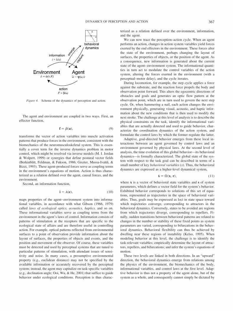
Armed with this array of concepts, let us return to the originalquestion of adaptive behavior in biological systems. In this sectionI propose an approach to goal-directed behavior at two levels ofanalysis (see Figure 4). The first level is that of the components ofthe system—the agent and environment—and their interactions inthe course of detecting information and controlling action, whichhave been referred to as the perception–action cycle (Kugler &Turvey, 1987; Warren, 1988). Local interactions between thesecomponents give rise to the global behavior of the system. Thesecond level of analysis is a low-dimensional description of thisglobal behavior, the behavioral dynamics (Fajen & Warren, 2003).My aim is to show how the behavioral dynamics both arise fromthe specifics of perception and action and reciprocally act toconstrain them.

Let us begin by supposing that the agent and the environmentcan be treated as a pair of coupled dynamical systems, with thefollowing equations of motion:

e � ��e, f )a � � (a, i), (8)

where e is a vector of environmental state variables, f is a vectorof external forces, a is a vector of agent state variables (whichdescribes the current state of the action system), and i is a vectorof informational variables. This is trivially true of the environment,which is governed by laws of physics � that can be expressed inthe form of differential equations. Change in the environment isthus a function of its current state together with any external forcesthat act on it.

Following the dynamical approach to action, I also assume thisto be the case for the agent. Specifically, the action system, with itsmany neuromuscular and biomechanical degrees of freedom, be-haves as a low-dimensional dynamical system for a given task(Saltzman & Kelso, 1987; Scholz & Schoner, 1999). Although thisformulation does not explicitly represent biological noise, stochas-tic models of coordination dynamics have been developed(Schoner, Haken, & Kelso, 1986). However, adaptive behaviordoes not consist in coordinated movement per se but in goal-directed action that is tailored to the environment. Hence, a fewcontrol variables must be left free to vary, which may be regulatedby perceptual information. Thus, an action is some function of thecurrent state of the action system together with informationalvariables i, according to a law of control �.

6 Conversely, an unstable limit cycle would repel the system away fromits closed orbit. Note that in a deterministic two-dimensional system,trajectories in the phase plane cannot cross, for the system cannot move intwo different directions from a given state.

366 WARREN

The agent and environment are coupled in two ways. First, aneffector function,

f � ��a, (9)

transforms the vector of action variables into muscle activationpatterns that produce forces in the environment, consistent with thebiomechanics of the neuromusculoskeletal system. This is essen-tially a cover term for the inverse dynamics problem in motorcontrol, which might be resolved via inverse models (M. I. Jordan& Wolpert, 1999) or synergies that define postural vector fields(Berkinblitt, Feldman, & Fukson, 1986; Giszter, Mussa-Ivaldi, &Bizzi, 1993). These agent-produced forces serve as coupling termsin the environment’s equations of motion. Action is thus charac-terized as a relation defined over the agent, causal forces, and theenvironment.

Second, an information function,

i � �(e), (10)

maps properties of the agent–environment system into informa-tional variables, in accordance with what Gibson (1966, 1979)called laws of ecological optics, acoustics, haptics, and so on.These informational variables serve as coupling terms from theenvironment in the agent’s laws of control. Information consists ofpatterns of stimulation at the receptors that are specific to theecological state of affairs and are therefore useful in controllingaction. For example, optical patterns reflected from environmentalsurfaces to a point of observation provide information about thelayout of surfaces, the properties of objects and events, and theposition and movement of the observer. Of course, these variablesmust be detected and used by perceptual systems that are tuned toparticular patterns of stimulation, with attendant issues of sensi-tivity and noise. In many cases, a presumptive environmentalproperty (e.g., euclidean distance) may not be specified by theavailable information or accurately recovered by the perceptualsystem; instead, the agent may capitalize on task-specific variables(e.g., declination angle; Ooi, Wu, & He, 2001) that suffice to guidebehavior under ecological conditions. Perception is thus charac-

terized as a relation defined over the environment, information,and the agent.

We can now trace the perception–action cycle. When an agentperforms an action, changes in action system variables yield forcesexerted by the end effectors in the environment. These forces alterthe state of the environment, perhaps changing the layout ofsurfaces, the properties of objects, or the position of the agent. Asa consequence, new information is generated about the currentstate of the agent–environment system. The informational quanti-ties in turn act to modulate the control variables of the actionsystem, altering the forces exerted in the environment (with aperceptual–motor delay), and the cycle iterates.

During locomotion, for example, the step cycle applies a forceagainst the substrate, and the reaction force propels the body andobservation point forward. This alters the egocentric directions ofobstacles and goals and generates an optic flow pattern at theobservation point, which are in turn used to govern the next stepcycle. Or, when hammering a nail, each action changes the envi-ronment physically, generating visual, acoustic, and haptic infor-mation about the new conditions that is then used to modify thenext stroke. The challenge at this level of analysis is to describe thephysical constraints on the task, identify the informational vari-ables that are actually detected and used to guide behavior, char-acterize the coordination dynamics of the action system, andformulate the control laws by which the former regulate the latter.

Adaptive, goal-directed behavior emerges from these local in-teractions between an agent governed by control laws and anenvironment governed by physical laws. At the second level ofanalysis, the time evolution of this global behavior—its behavioraldynamics—is formally characterized. The global state of the sys-tem with respect to the task goal can be described in terms of asmall number of key behavioral variables (x). Thus, the behavioraldynamics are expressed as a higher-level dynamical system,

x � �x, r, (11)

where x is a vector of behavioral state variables and s of systemparameters, which defines a vector field for the system’s behavior.Exhibited behavior corresponds to solutions of this set of equa-tions, represented as trajectories in the space of behavioral vari-ables. Thus, goals may be expressed as loci in state space towardwhich trajectories converge, corresponding to attractors in thebehavioral dynamics. Conversely, states to be avoided are regionsfrom which trajectories diverge, corresponding to repellers. Fi-nally, sudden transitions between behavioral patterns are related tochanges in the number or stability of these fixed points as systemparameters are varied, corresponding to bifurcations in the behav-ioral dynamics. Behavioral flexibility can thus be achieved bydwelling near these regions of instability (Kelso, 1995). Whenmodeling behavior at this level, the challenge is to identify thetask-relevant variables; empirically determine the layout of attrac-tors, repellers, and bifurcations; and infer the system’s equations ofmotion.

These two levels are linked in both directions. In an “upward”direction, the behavioral dynamics emerge from relations amongthe physics of the environment, the biomechanics of the body,informational variables, and control laws at the first level. Adap-tive behavior is thus not a property of the agent alone, but of thesystem as a whole, and consequently cannot simply be dictated by

Figure 4. Schema of the dynamics of perception and action.


the nervous system. Rather, the role of the nervous system is toadjust the mapping between informational variables and controlvariables (i.e., control laws) so as to give rise to stabilities in thebehavioral dynamics that correspond to the intended behavior. Ina “downward” direction, attractors in the behavioral dynamics actto capture the perception–action cycle. Specifically, the morphol-ogy of this vector field has behavioral consequences that can beperceived, such as sensing one’s own energy expenditure, thevariability of action, or task success. These observations provide afeedback that serves to fix control laws and index parameter valuesthat yield effective behavior. Perception and action systems thusmanifest the properties of upward and downward causality that arecharacteristic of emergent behavior and self-organization (Bar-Yam, 2004; Haken, 1977).

As the agent interacts with the world, the behavioral dynamicsare likely to evolve. Previous work on coordination dynamics hasfocused on fairly simple tasks with stationary dynamics, such asrhythmic movement or bimanual coordination. But in more com-plex adaptive behavior, the dynamics may depend on the agent’sinteraction with the environment. The landscape of attractors andrepellers can shift as the agent navigates through it, and bifurca-tions open up new behavioral avenues as others are closed off. Thetrajectory of behavior thus unfolds as agent and environmentinteract, guided by tracking the evolving stabilities. Moreover,because the system is nonlinear, this behavioral trajectory is highlysensitive to initial conditions and susceptible to noise. The body isa complex system with many interdependent neuromusculoskeletalcomponents, and these processes contribute to high-dimensionalcomplexity in what is essentially a low-dimensional action pattern(Newell & Corcos, 1993). Such effects can cascade through abehavioral sequence, altering the initial conditions for the nextaction and sending behavior down qualitatively different paths(Van Orden, Holden, & Turvey, 2003). Such historical contin-gency can make individual behavior notoriously difficult to pre-dict, particularly in noisy biological systems. Consequently, re-searchers may need to be satisfied with theories that capture thedynamical “deep structure” of behavior—the morphology of at-tractors, repellers, and bifurcations for a given task—rather thanone that can precisely predict individual behavior on particularoccasions.

In summary, a formal description of behavior requires identify-ing a system of differential equations whose vector field corre-sponds to the observed pattern of behavior, with attractors corre-sponding to goal states, repellers to avoided states, andbifurcations to qualitative behavioral transitions. But an explana-tion of adaptive behavior further requires showing how thesebehavioral dynamics arise from interactions among the system’scomponents, that is, how a stable solution is codetermined byphysical and informational constraints. Ultimately, it must beshown how behavior is self-organized through feedback from thebehavioral dynamics.

Control Laws

The control problem with which we began is now recast in termsof the dynamics of the agent–environment system. From theagent’s perspective, the problem becomes one of tweaking thedynamics of the system in which it is embedded so as to enact

stabilities for the intended behavior. The lever at the agent’sdisposal is the law of control, and here lies the psychological heartof the matter.

Typically, a control law in perception and action is thought of asa mapping from task-specific information to a movement variable,m � f (i) (see Warren & Fajen, 2004). But the way in whichinformation can influence movement is by means of modulatingthe dynamics of the action system. Thus, it is more appropriate towrite control laws as a function in which informational variablesmodulate the control variables of a dynamical system:

a � �(a, i). (12)

This control law has two implicit parts: First is a dynamical systemthat represents the organization of the action system for a partic-ular task, a � �(a), which Kelso (1995) referred to as the “in-trinsic dynamics.” Second is an informational coupling term inwhich optic, acoustic, haptic, and so forth variables i modify thecontrol variables of the dynamical system. The resulting controllaw does not specify the kinematics of movement per se but ratherrelaxes to an attractor in the action variables a that corresponds tothe desired action. The effector function � then converts this limitvalue of the action variable into muscle activation and thence limbkinematics and endpoint forces, given the biomechanics of themusculoskeletal system.

For information to modulate the action system, it is essential thatinformational variables be commensurate with control variables.That is, low-dimensional informational terms, which reflect higherorder relations among many elementary variables, must map tolow-dimensional control terms, which reflect higher order relationsamong the many degrees of freedom of the musculoskeletal sys-tem. To be commensurate, these informational and control termsmust have the same dimensions and are typically expressed in thesame variables.

A pertinent example is the optic flow field, the pattern of opticalmotion produced at a moving point of observation during terres-trial locomotion (Gibson, 1950; Warren, 2004). Here, relationsdefined over many elementary local motions form a global flowpattern, which contains a focus of expansion in the direction ofself-motion or heading. The focus of expansion constitutes ahigher order variable that specifies the current heading direction(azimuth angle), relative to which the directions of goals andobstacles can also be defined. Thus, high-dimensional local mo-tions are compressed into a low-dimensional variable that is com-mensurate with behavior. On the action side, gait patterns reflectthe compression of many neuromusculoskeletal degrees of free-dom into a task-specific organization, such that the action systembehaves as a low-dimensional dynamical system with a few freecontrol variables. One of these control variables is the direction offorce applied against the ground, which determines the currentheading direction. The informational and control terms are thus ofthe same dimensionality and are expressed in the same variable(azimuth angle), such that the direction of a goal with respect to thecurrent heading can directly control the direction of force appli-cation. I develop this case in some detail below. Other controlrelations may not be quite as transparent, of course, and caninvolve more complex variables and scaling factors. But the pointis that, for a given task, the agent need only map low-dimensional

368 WARREN

information to low-dimensional control variables, thereby simpli-fying the control problem.7

Control variables may be of two types: state variables or pa-rameters. In addition, information may regulate a control variableby three possible manners of coupling: continuous modulation,periodic adjustment, or discrete resetting. Crossing control vari-ables with manners of coupling yields six logically possible con-trol modes that an agent can exploit to shape the dynamics for thetask at hand, which are illustrated below.

State Control

First, information may influence the state variables of a system(e.g., its position and velocity). This is achieved by allowinginformational quantities to contribute to the dynamics, altering theattractive states (Schoner & Kelso, 1988b; Schoner, Zanone, &Kelso, 1992). In the simple one-dimensional system of Equation 2,for instance, the intrinsic dynamics possess a fixed point at a � 0.However the goal state may be at another value that is specified byinformation, a � i. Adding an informational coupling term ci,

a � �ra � ci, (13)

shifts the attractor along the abscissa toward i. The magnitude ofthe shift is determined by the relative strength of the informationand action terms (determined by coefficients c and r). A specialcase occurs when c � r, so information about the goal statecompletely determines the resulting fixed point:

a � �r(a � i). (14)

In this case, the attractor shifts to the specified location at a � i,and the system relaxes to the goal state. An early example is theequilibrium-point model of single joint movement (Asatryan &Feldman, 1965; Latash, 1993). Note that i might be discretely resetto a fixed value so the attractor is stationary (Asatryan & Feld-man’s, 1965, original proposal), continuously modulated so thatthe attractor location evolves in time (an equilibrium point trajec-tory), or adjusted periodically so that the attractor regularly shiftsposition (yielding a rhythmic movement). Information and controlare commensurate because the informational variable specifies thegoal state of the system in the terms of the state variable a.

An illustrative case of state control is provided by Schoner’s(Dijkstra, Schoner, & Gielen, 1994; Schoner, 1991) model of thevisual regulation of standing posture. The intrinsic postural dy-namics are modeled as a second-order system similar to Equation6, with a fixed point at (x, x) � (0, 0) corresponding to uprightstance. Visual information about postural sway is provided by therelative rate of optical expansion e(x, t) � �/�, the inverse of Lee’s(1976; Lee & Lishman, 1975) time-to-contact variable, where � isthe visual angle of a frontal surface patch. Information is treated asa continuous forcing function, such that a coupling term is addedinto the dynamics,

x � ��x � �2x � �Qt � ce(x, t) (15)

where c is the coupling strength, � is the damping, � is theeigenfrequency of the postural system, and �Qt is a stochasticterm that introduces random fluctuations. Information effectivelyshifts the resulting fixed point along the x dimension, such that

optical expansion leads to backward postural acceleration, andoptical contraction to forward acceleration. Because the optic flowis itself determined by postural position and velocity, the informa-tion is defined in the same terms as the control variables.

Parametric Control

Second, information may modulate the parameters of a system,affecting its state indirectly. For the one-dimensional system ofEquation 2, this is equivalent to adding the informational couplingterm i to parameter r, so the control law becomes

a � �(r � i)a. (16)

In this case, the parameter affects the slope of the function inFigure 1a and hence the relaxation time to the fixed point, whoselocation remains constant. For the nonlinear system of Equation 3,on the other hand, modulation of the control parameter can take thesystem through a bifurcation, changing its stability and the numberof fixed points.

In a two-dimensional system such as Equation 4, discrete reset-ting of the stiffness parameter k changes its frequency of oscilla-tion and in some cases its amplitude as well (Kay, Kelso, Saltz-man, & Schoner, 1987). Continuous modulation of the parametercan also amplify the system’s oscillation, a phenomenon known asparametric excitation (Hayashi, 1964; Nayfeh & Mook, 1979). Afamiliar example is pumping on a swing: Periodically raising andlowering one’s center of mass decreases and increases the effectivelength (and hence the natural frequency) of the pendulum, boostingits amplitude (Post, 2000).8

Kay and Warren (1998, 2001) first demonstrated parametricexcitation in biological coordination by showing that gait synchro-nizes to posture during walking (see also Jirsa, Fink, Foo, & Kelso,2000). Specifically, when postural sway is driven by an oscillatingvisual display at various frequencies, the step cycle becomesentrained to the visual driver at specific integer mode lockingratios (1:1, 2:1, 3:2, etc.). Such superharmonic entrainment, inwhich the natural frequency of the driven oscillator (gait) is higherthan the frequency of the driver (visual display), is only stable inparametrically forced systems. The results are consistent withcontinuous modulation of a gait “stiffness” parameter.

In summary, control laws involve mapping informational vari-ables to state variables or parameters of a dynamical system, withthree manners of coupling. This offers six possible control modesby which information can influence the dynamics of behavior.

Stabilization of Goal-Directed Behavior

The function of perception and action is to stabilize behavior onthe goal for a given task while maintaining adaptive flexibility. To

7 For simplicity, informational variables themselves appear in the con-trol law of Equation 12, ignoring for the moment the complexities of thedetection process. In principle, this term could be expanded to incorporatea perceptual transduction function, so that the registered values of thesevariables appear in the control law.

8 A swing actually combines parametric and state control, becausepumping both changes the length of the pendulum and shifts the center ofmass backward and forward, changing its state.


this end, control laws use information to modulate the dynamics ofthe action system. The behavioral outcome is a consequence of theinteraction among the control laws, the biomechanics of the body,and the physics of the environment. In many instances, thesephysical constraints can simplify the control problem by determin-ing stable or preferred solutions. The degree to which a stablesolution is sitting in the physics of the task awaiting discovery oris created by the appropriate use of information depends on thenature of the task. The agent contributes to the solution by dis-covering the relevant physical and informational quantities andidentifying control laws that yield successful, stable behavior.Finally, to avoid getting locked into a rigidly stable solution, theagent also uses information to maintain adaptive flexibility (Beek,1989; Kelso, 1995).

A taxonomy of tasks can be developed on the basis of theirinherent physical stability. First are those that possess passivelystable solutions given by the physics of the task, for example, apoint attractor or limit cycle. This is perhaps the simplest case,because the solution is highly constrained and can be discoveredvia perceptual–motor exploration. Second are tasks that are inher-ently unstable, such as those characterized by an unstable fixedpoint. These require active stabilization, by means of control lawsthat use information to counteract the physical instability. This isa more challenging case because, although the solution is physi-cally constrained in the sense that the goal state is picked out bythe fixed point, the agent must discover the relevant informationand identify an effective control law. Moreover, there is no guar-antee that a realizable solution exists. Third are tasks that areneutrally stable, with no intrinsic fixed points. A stable solutionthus depends on identifying informational variables that allow thegoal to be realized. This case is difficult because, in the absence ofphysical constraints, the solution space is a level playing field untilfixed points are created by the appropriate use of information. Toshow the process of stabilization at work, I present examples of thethree basic cases from the recent literature.

Stabilizing a Passively Stable System: Follow theBouncing Ball

Consider first a deceptively simple task that is a textbookexample in nonlinear dynamics: bouncing a ball on a racquet inone (vertical) dimension. As racquet frequency increases, thebouncing ball system actually exhibits the period-doubling route tochaos (Guckenheimer & Holmes, 1983; Tufillaro, Abbott, &Reilly, 1992). But our interest is in stable Period 1 bouncing, inwhich the period of the ball is equal to one racquet period and itbounces to a constant height. In the purely passive case, theracquet oscillates sinusoidally with a constant frequency (�) andamplitude (A) without active control, and the ball falls with grav-itational acceleration (g) and rebounds from the racquet with acoefficient of restitution (�) less than 1.

Counterintuitively, Period 1 bouncing is passively stable whenimpact occurs during the decelerative phase of racquet motion(Dijkstra, Katsumata, de Rugy, & Sternad, 2004; Schaal, Sternad,& Atkeson, 1996)—that is, in the upward swing between theracquet’s approximately horizontal position (where its velocity ismaximum and deceleration is zero) and its highest position (whereits velocity is zero and deceleration is maximum). Specifically,

bouncing is qualitatively stable when impact acceleration is be-tween zero and a negative value equal to �2g(1 � �2)/(1 � �)2

and is maximally stable in a smaller region within this range. Inthis regime, if the system is perturbed, it will self-correct to aconstant impact acceleration and bounce height. This means thatthe ball can be bounced blindly as long as the racquet keeps goingat a constant frequency, requiring no sensory information.

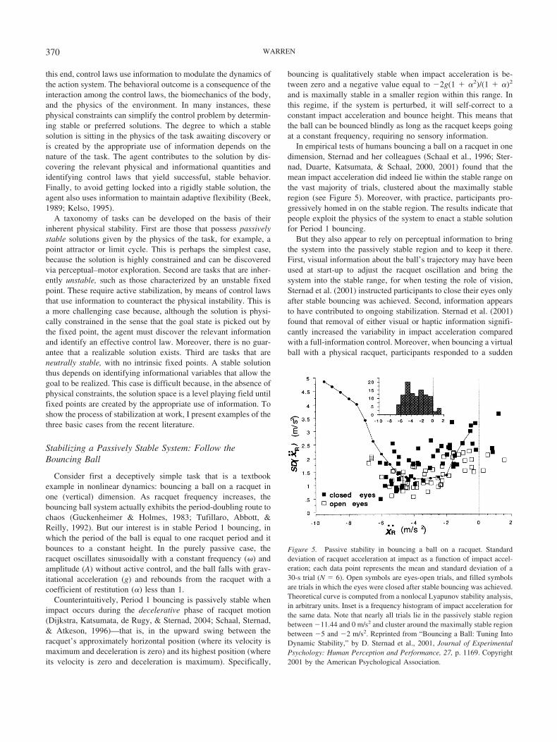
In empirical tests of humans bouncing a ball on a racquet in onedimension, Sternad and her colleagues (Schaal et al., 1996; Ster-nad, Duarte, Katsumata, & Schaal, 2000, 2001) found that themean impact acceleration did indeed lie within the stable range onthe vast majority of trials, clustered about the maximally stableregion (see Figure 5). Moreover, with practice, participants pro-gressively homed in on the stable region. The results indicate thatpeople exploit the physics of the system to enact a stable solutionfor Period 1 bouncing.

But they also appear to rely on perceptual information to bringthe system into the passively stable region and to keep it there.First, visual information about the ball’s trajectory may have beenused at start-up to adjust the racquet oscillation and bring thesystem into the stable range, for when testing the role of vision,Sternad et al. (2001) instructed participants to close their eyes onlyafter stable bouncing was achieved. Second, information appearsto have contributed to ongoing stabilization. Sternad et al. (2001)found that removal of either visual or haptic information signifi-cantly increased the variability in impact acceleration comparedwith a full-information control. Moreover, when bouncing a virtualball with a physical racquet, participants responded to a sudden

Figure 5. Passive stability in bouncing a ball on a racquet. Standarddeviation of racquet acceleration at impact as a function of impact accel-eration; each data point represents the mean and standard deviation of a30-s trial (N � 6). Open symbols are eyes-open trials, and filled symbolsare trials in which the eyes were closed after stable bouncing was achieved.Theoretical curve is computed from a nonlocal Lyapunov stability analysis,in arbitrary units. Inset is a frequency histogram of impact acceleration forthe same data. Note that nearly all trials lie in the passively stable regionbetween �11.44 and 0 m/s2 and cluster around the maximally stable regionbetween �5 and �2 m/s2. Reprinted from “Bouncing a Ball: Tuning IntoDynamic Stability,” by D. Sternad et al., 2001, Journal of ExperimentalPsychology: Human Perception and Performance, 27, p. 1169. Copyright2001 by the American Psychological Association.

370 WARREN

change in g or � within one cycle (Siegler, Mantel, Warren, &Bardy, 2003). Indeed, de Rugy, Wei, Muller, and Sternad (2003)observed that when � was randomly perturbed on a single bounce,participants adjusted the racquet period to bring the ball back intothe stable range on the next impact. They successfully modeledthis behavior with a “period controller,” which uses the perceivedperiod of the ball’s flight to modulate the period of racquet motion.These results indicate that visual information is used to regulateracquet motion on a cycle-to-cycle basis, suggesting that ballbouncing involves a mixed regime that blends passive stability andactive control. In addition, bouncing can be sustained outside thestable region with positive impact accelerations, by using visionalone to actively stabilize the system (Siegler et al., 2003).

To adjust the period of racquet motion, it is reasonable toassume that observers use visual information about the duration ofthe ball’s flight, specifically, the time (tc) remaining until the ballwill arrive the height of the previous contact (hc). Several candi-date variables that specify this arrival time can be identified. First,the arrival time can be determined from the peak height of theball’s trajectory (hp), given that g is known:

tc � �2hp/g.

Second, the arrival time can be predicted from the ball’s launchvelocity (v0), given that g is known: tc � v0/g. Third, the arrivaltime from the peak of the ball’s trajectory is equal to the first halfperiod of the ball’s flight: tc � /2. The advantage of this variableis that it holds irrespective of the gravitational constant and thusdoes not depend on a known g. Finally, arrival time is alsospecified haptically because the flight period is related to the forceat impact, which also depends on a known g. Siegler et al. (2003)found that participants recover from a sudden change in g asquickly as they do from a sudden change in �, indicating thatvisual control does not depend on a known g. Furthermore, theyadapt to a change in g by adjusting both the racquet’s period andamplitude but adapt to a change in � by adjusting only amplitude.The results are consistent with the use of information about theball’s flight period to control the period of racquet motion.

The behavioral dynamics of the bouncing task can thus beconceptualized as follows. The environment consists of the ball–racquet system in a gravitational field with constants g and �,governed by the mechanics of falling bodies and collisions (�).Given the task of Period 1 bouncing, the action system is organizedas a nonlinear limit-cycle oscillator generating vertical periodicmovements of the arm. A control variable such as the stiffnessparameter scales the period of oscillation. These two dynamicalsystems are coupled mechanically by the force applied to the balland informationally by optic (and haptic) variables that specify theball’s flight period. The control law (�) uses these variables tomodulate the stiffness parameter on each cycle, so that the racquetperiod matches the specified ball period. At the level of thebehavioral dynamics, these cyclic interactions have regions ofpassive stability with minimal active adjustments, which feed backduring learning to capture the preferred impact acceleration andphase. The stable solution for bouncing a ball on a racquet thustakes advantage of both physical constraints, which define passivestability, and informational constraints, which allow the agent tofind and sustain the stable regime.

Active Stabilization of an Unstable System: PoleBalancing

Now consider the problem of functionally stabilizing an unsta-ble fixed point. A good example is the task of balancing aninverted pendulum, a staple of control theory (Barto, Sutton, &Anderson, 1983; Kwakernaak & Sivan, 1972). A pole will balanceunaided if its angle to the vertical (�) is precisely zero, but givena slight perturbation it will fall with an angular acceleration in-versely proportional to its length. With a bit of practice, people canlearn to balance a pole upended on one hand (or a chair on thechin) by applying appropriate horizontal forces to its base.

The control-theoretic approach to such a planar cart–pole prob-lem is to derive a linear control strategy in which the horizontalforce F is computed as a weighted sum of the state variables of thesystem, typically the angle (�) and angular velocity (�) of the poleand the position (x) and velocity (x) of the cart that supports it. Theproblem thus boils down to determining fixed coefficients for eachstate variable, given the mechanics of a particular pendulum. Thisgenerally results in successful solutions in which the pole oscil-lates about the vertical without falling. But do biological systemsstabilize an inverted pendulum in this manner? In the present view,rather than a general solution based on elementary state variables,it is likely that people find a control law that maps higher orderinformational variables into higher order control variables.

To address these questions, Foo, Kelso, and Guzman (2000)recorded people’s behavior as they tried to balance a pole attachedto a cart that was moved by hand along a horizontal track. Duringsuccessful 30-s trials, the pole tended to oscillate by a few degreesin a regular pattern of overshooting the vertical and being recov-ered again by a hand adjustment, occasionally punctuated byundershooting. The authors hypothesized a higher order informa-tional variable called “time-to-balance” (bal), an angular versionof Lee’s time-to-contact variable (Lee, Young, & Rewt, 1992).Specifically, the ratio between the current pole angle (with respectto the vertical) and its rate of change specifies the time remaininguntil the pole arrives at the vertical position, if angular velocityremains constant:

bal ��

�. (18)

Foo et al. (2000) pointed out that rate of change in this variable(bal) can be interpreted in terms of the angular deceleration of thepole as it approaches the vertical (Lee, 1976). A value in the range0 � bal � 0.5 specifies that the current deceleration is too great,and if maintained, the pole will undershoot the vertical and couldfall. A value of bal � 0.5 indicates that the current deceleration,if held constant, will bring the pole to rest precisely at the vertical.However, because this fixed point is unstable the subsequentmotion of the pole would be unpredictable, so control wouldbecome reactive. A value in the range 0.5 � bal � 1.0 specifiesthat the current deceleration is too low and the pole will overshootthe vertical—but it will remain controllable with subsequent ad-justments. A bal � 1.0 corresponds to a constant angular velocity,and bal � 1.0 specifies that the pole is accelerating toward thevertical, which will lead to a large overshoot. If maintained in thisregime over several cycles, the amplitude of oscillation wouldincrease and the system would become uncontrollable.


Consistent with this analysis, the data show that prior to over-shoots, the time series of bal hovers between 0.87 and 0.97 at peakhand velocity. In contrast, prior to undershoots the mean values ofbal are between 0.18 to 0.36 at peak hand velocity. Foo et al.(2000) argued that the hand’s peak velocity is a critical controlpoint at which information is used to initiate a new adjustment,such as reversing hand direction or launching a new movement inthe same direction.

These findings lead Foo et al. (2000) to propose a visual controlstrategy based on bal: To stabilize an inverted pendulum, keep bal

between 0.5 and 1.0 at peak hand velocity. To implement thisstrategy, they defined a control law in which the force to be appliedby the hand (scaled to the length and mass of the pendulum) is alinear weighted function of pole angle and hand position,

F � �bal� � �x, (19)

where � is a constant as in a standard controller. Stabilization isachieved by using time-to-balance information bal to periodicallymodulate the “stiffness” parameter � at each control point in thecycle. In brief, � is adjusted by an amount based on how far thecurrent value of bal is outside the interval {0.5, 1.0}. The resultingforce returns bal into the controllable range, keeping the polebalanced. Simulations of this strategy applied to a model cart–polesystem produced time series that are qualitatively similar to thehuman data, including antiphase coordination between hand andpole velocity, bal values near zero for most of a cycle, and bal

values near 1.0 at peak hand velocity.This analysis can be cast into the behavioral dynamics frame-

work as follows. The environment is governed by the physics ofthe inverted pendulum in a gravitational field (�). The actionsystem is organized as an oscillator that generates horizontalmovements of the hand, with both state and parametric controlvariables. The agent is mechanically coupled to the pole via theforce exerted on the cart and informationally coupled via visualinformation about the pole angle � and bal and visual or hapticinformation about hand position x. The control law (�) uses thisinformation to continuously modulate the state variables determin-ing applied force F and to periodically adjust the “stiffness”parameter �. At the level of the behavioral dynamics, this givesrise to small periodic fluctuations in pole angle, stabilizing it in theneighborhood about the fixed point at (�, �) � (0, 0).

Thus, the pole is dynamically balanced by exploiting a combi-nation of physical and informational constraints that allow theagent to functionally stabilize the system. Although the invertedpendulum is physically unstable, the solution to the pole balancingproblem is still constrained by the existence of an unstable fixedpoint that clearly picks out a goal state.

Active Stabilization of a Neutrally Stable System: Braking

In the previous example, the physics of the inverted pendulumlimits the solution space for stabilizing the system. But in manyperceptual–motor tasks, the physical and biomechanical con-straints are weak or nonexistent. The system is thus neutrally stablein the sense that there are no intrinsic fixed points and no inher-ently preferred or unpreferred states. However, informational con-straints can play a role analogous to physical constraints when the

agent can identify higher order variables that permit the functionalstabilization of a behavioral pattern.

A good example is provided by Lee’s (1976) theory of the visualcontrol of braking. Imagine that the agent is traveling toward anobstacle at a distance z, and the task is to decelerate to a stop rightin front of it, such that (z, z) � (0, 0). The intrinsic physics of thesituation offer little constraint, for left to itself the body or vehiclewill continue to hurtle toward a collision, slowing slightly due tofriction. There is no fixed point in this case because the position atwhich the vehicle will finally stop depends entirely on initialconditions. Thus, the active stabilization of braking at (z, z) � (0,0) must rely upon informational constraints.

Lee (1976) based his analysis of braking on the variable,which denotes the ratio of an object’s visual angle (�) over its rateof change (�) and corresponds to the first-order time to contact(limits to this analysis have been discussed by Tresilian, 1990,1999). The time derivative of this variable () specifies the ade-quacy of the current deceleration, as just described for the case ofpole balancing. Specifically, a value of � �1.0 indicates aconstant velocity approach and hence an eventual crash.9 A valuein the range �1.0 � � �0.5 specifies that the current deceler-ation is too low and, if maintained, would result in a collision, sothe agent should increase the brake. A � �0.5 indicates that thecurrent deceleration will bring the agent to a precise stop at theobstacle if held constant. And finally, a � �0.5 specifies that thecurrent deceleration is too high and would lead one to stop short ofthe obstacle, so the agent should decrease the brake. Thus, ��0.5 corresponds to the boundary between a crash state and a safestate if the current deceleration is maintained. Note that the visualsystem need not be sensitive to per se, which depends ondetecting an optical acceleration, but could be sensitive to a suf-ficiently small difference �, which depends on detecting a thresh-old change in optical velocity.

Yilmaz and Warren (1995) experimentally tested several strat-egies as well as alternative hypotheses based on the simple rate ofexpansion (�) or computing deceleration from spatial variables.Participants viewed an interactive display of approach to a roadsign, with or without a ground plane that added information aboutspeed and distance. They controlled their deceleration with a linear“brake,” a spring-loaded mouse in which deceleration was propor-tional to position. The data were quite consistent with a strategy,with an overall mean of �0.51. However, the time series ofbraking behavior revealed that participants did not hold constantat �0.5, as some have suggested (Kaiser & Phatak, 1993; Kim,Turvey, & Carello, 1993; Lee, 1976), but rather made a series ofbrake adjustments at a rate of about one per second. A detailedanalysis showed that the direction and magnitude of each adjust-ment depended upon the current value of . This relationship isrepresented in Figure 6, which plots the mean change in duringa brake adjustment as a function of the value of at the onset ofthe adjustment. The slope of the function is exactly �1.04, and itcrosses the abscissa at a value of � �.52 (r � .98). This meansthat if � �0.52, participants increase their deceleration, and if

9 The signs of these values are negative, consistent with Lee’s (1976)original analysis. Otherwise, this is analogous to the pole-balancing anal-ysis in the preceding section.

372 WARREN

� �0.52, they reduce their deceleration—by an amount that onaverage brings back to a criterial value of �0.52.10

Note that Figure 6 actually represents the phase portrait of theinformational variable . It reveals that participants stabilize theirbraking behavior by enacting a point attractor in the dynamics of. This is not an arbitrary solution but reflects the informationalstructure of the task, specifically the relation between higher ordervariables and deceleration conditions, which corresponds to theboundary between a crash state and a safe state. Note also thatbraking is effected via periodic discrete adjustments of a controlvariable, in this case the state variable of brake position, whichdirectly determines the braking force and deceleration.

The visual control of braking can be placed in the behavioraldynamics framework as follows. The environment consists of theobstacle, the vehicle and brake dynamics, and the road surface,governed by the laws of physics (�). The action system is pre-sumably organized as a second-order system similar to Equation 6,with an equilibrium point at a desired brake position x. The agentis mechanically coupled to the environment via force exerted onthe brake and informationally coupled via . Provisionally, thecontrol law can be modeled by a difference equation in which the

change in brake position (�x) is proportional to the distance of from its criterial value,

�x � b(�0.52 � ) � �, (20)

where depends on brake position x, b scales the amplitude ofbrake adjustment, and � is a noise term that produces random over-and undercorrection. This works because is roughly proportionalto deceleration and hence to brake position during most of thecontrolled approach. The control law thus uses the current value of(�0.52 � ) to regulate the change in brake position. This exertsa braking force on the vehicle and produces a deceleration accord-ing to physical laws, which in turn affects the informationalvariable . At the level of the behavioral dynamics, this use ofinformation serves to stabilize braking behavior in the neighbor-hood of (z, z) � (0, 0).

These three examples illustrate how biological systems useinformation to find a passively stable solution, to actively stabilizean unstable system, or to actively stabilize a neutrally stablesystem. In the first case, a solution is given by the physics of thetask and can be discovered through perceptual–motor exploration.In the second case, information is used to stabilize an unstablesystem, but the solution is narrowly constrained by the physics ofthe task. Finally, in the third case, information is used to enactstable states based on the informational structure of the task.Information may be used to influence a state variable, such asbrake position, or to modulate a parameter, such as the stiffness ofthe oscillator in bouncing or pole balancing. Finally, such controlvariables may be modulated continuously, periodically adjusted oneach cycle, or discretely reset to a fixed value. Empirical researchon such whole agent–environment systems is required to modelthe specifics of the perception–action cycle and to formally char-acterize the behavioral dynamics of a given task.

A Case Study: Behavioral Dynamics of Locomotion

The time has come to put these concepts to work. The goal ofthis section is to show how adaptive behavior actually arises fromagent–environment interactions by pursuing a model system insome depth. Fajen and I have recently developed a theory of thedynamics of locomotor behavior, in which the elements of thecurrent framework have been modeled and empirically tested(Fajen & Warren, 2003, 2004; Fajen, Warren, Temizer, & Kael-bling, 2003). Our approach to modeling human locomotor pathformation is influenced by the work of Schoner et al. (1995) on acontrol system for mobile robots.

Imagine yourself walking through Grand Central Station in NewYork City. To reach the exit, you must adopt a route through acomplex dynamic environment. First, you must steer toward astationary goal—the exit. At the same time, you must avoidstationary obstacles, such as benches and luggage. Worse, you alsohave to avoid moving obstacles, such as baggage carts and otherpassengers—some of which are simultaneously trying to avoidyou. Along the way, you might spot a passing acquaintance and try

10 There are small individual differences in this criterial value, indicatingmore risky or conservative braking, and in the slope of the line, indicatinga tendency to over- or undercorrect.

Figure 6. Active stabilization of a neutrally stable system: Phase portraitfor braking to stop at an obstacle. Mean change in during a brakeadjustment as a function of at the onset of the adjustment, based on 4,800trials (N � 12). Note that the regression line indicates a point attractor ata of �0.52, close to the theoretical value of �0.50, with a slope of �1.04(r � .98). Reprinted from “Visual Control of Braking: A Test of the Hypothesis,” by E. H. Yilmaz and W. H. Warren, 1995, Journal ofExperimental Psychology: Human Perception and Performance, 21, p.1010. Copyright 1995 by the American Psychological Association.


to intercept this moving target—which may also seek to interceptor evade you. Locomotion in a complex changing environmentrequires integrating these four elementary behaviors (stationarygoal, stationary obstacle, moving target, moving obstacle) to gen-erate a locomotor path, a surprisingly difficult task that mobilerobots have yet to master. Below I show that human locomotorpaths can be understood as dynamic trajectories that unfold onlineas the agent interacts with its environment.

The path of locomotion is unconstrained, which puts it in theclass of neutrally stable systems that must be functionally stabi-lized by information. Most interesting, the dynamics evolve as theagent moves through the environment, making this the first case inwhich the dynamical approach has been applied to a nonstationaryreal-world behavior. To address this problem, Fajen and I (Fajen &Warren, 2003) developed a model of the behavioral dynamics oflocomotion. In this research program, we record human walking insimple cases and use the data to specify a component model foreach of the four basic behaviors. We then fix the parameter valuesand attempt to predict locomotor paths in more complex situationsby linearly combining these components. Finally, we infer possiblecontrol laws that give rise to the observed behavior. If we canformalize the locomotor dynamics for an individual agent, thismay ultimately allow us to model interactions among multipleagents in a complex environment like Grand Central Station.

Steering to a Goal

Recall that exhibited behavior can be analyzed as a trajectory inthe state space of behavioral variables, where attractors correspondto goal states and repellers to avoided states. The desired aim is todescribe the behavioral dynamics of the task by formalizing adynamical system with a vector field that corresponds to theobserved behavior.

Consider first the task of steering to a stationary goal. Thebehavioral variables are defined as the current heading direction �with respect to an arbitrary reference axis (see Figure 7) and thecurrent turning rate �. Walking speed is fairly constant in the data,so for the moment assume a constant speed v. From the agent’scurrent (x, z) position, a goal lies in the direction �g at a distancedg. The simplest description of steering is to bring the headingerror, the angle between the current heading direction and the goaldirection, to zero (� � �g � 0). The goal direction is thus anattractor of heading in state space at (�, �) � (�g, 0). The distanceof the goal (or equivalently, its time to contact) might also beexpected to influence steering, because the agent may need to turnfaster to hit a nearer goal.

Because the agent is embodied, the physical body must undergoangular acceleration to change its direction of travel, and thus it isreasonable to assume that a description of steering behavior re-quires at least a second-order system. To get an intuition, imaginethat the agent’s current heading direction is attached to the goaldirection by a damped spring (see Figure 7). Angular accelerationtoward the goal direction would thus depend on the stiffness of thespring and be resisted by the damping. To make the attractivenessof the goal depend on its distance, the goal distance is used tomodulate the spring stiffness parameter continuously.

To specify these functions, a series of studies determined howthe locomotor path is influenced by the directions and distances of

goals and obstacles (Fajen & Warren, 2003). The research wascarried out in the Virtual Environment Navigation Lab (VENLab)at Brown University, a 12 m � 12 m room in which a participantcan walk freely wearing a head-mounted display (60° horizontal �40° vertical) while head position is recorded with a sonic–inertialtracking system. On each trial, the participant walked forward ona textured ground plane for 1 m, then a goal post appeared, and thetask was simply to walk to the goal. The first experiments variedthe initial heading error (0° to 25°) and goal distance (2 m to 8 m).

The data revealed that participants turned onto a straight path tothe goal (see Figure 8a) but did so more rapidly when the goal hada larger heading error or was at a closer distance. The time seriesof heading error showed that it converged to zero from all initialconditions (see Figure 8b), with an angular acceleration that in-creased linearly with heading error and decreased exponentiallywith goal distance. Thus, the goal direction does in fact behave likean attractor of heading.

We modeled this behavior with an angular version of the “mass–spring” equation (Equation 4), in which angular acceleration � isa function of both heading error (� ��g) and goal distance (dg),

� � �b� � kg(� � �g)(e�c1dg � c2). (21)

The “damping” term indicates that the resistance to turning isproportional to the turning rate; the b parameter determines theslope of this function, expressing the ratio of damping to bodymass (in units of s�1). The “stiffness” term reflects the finding thatangular acceleration increases linearly with heading error, at leastover the tested range of �25° to �25°.11 The kg parameterdetermines the slope of this function and hence the attractivenessof the goal, expressing the ratio of stiffness to mass (in units of

11 It is interesting that Reichardt and Poggio (1976) determined a similarfunction for steering in the housefly that was also linear over this range.

Figure 7. Definition of variables for locomotor behavior: Heading direc-tion in an extrinsic coordinate frame �, direction of goal or obstacle �, andheading error in an intrinsic coordinate frame � � � � �. Steering behavesas though the heading direction were attached to the goal direction by aspring with stiffness k and damping b.

374 WARREN

s�2). Finally, the attractiveness of the goal decreases exponentiallywith distance, where c1 determines the rate of decay and c2 aminimum value (to ensure that one will steer toward distant goals).The slope of the “stiffness” function is thus modulated by distance.Least squares fits to the mean time series of heading error yieldedparameter values of b � 3.25, kg � 7.50, c1 � 0.40, and c2 � 0.40.

Simulations of the experimental conditions generate locomotorpaths that are very close to the human data (see Figure 9a) and timeseries of heading error that converge to zero in a similar manner(see Figure 9b). The fits to the mean time series accounted for aproportion of .980 of the variance, indicating that model behavioris highly similar to the mean human behavior. Thus, the modelsuccessfully captures the basic form of walking to a goal, in whichthe goal direction behaves like an attractor of heading whosestrength increases with angle and decreases with distance. Al-though four free parameters may seem to be overkill, it turns outthat simpler models do not account for the observed variation inhuman paths. Recall as well that the modeling strategy is to fixthese values and predict behavior in more complex environmentswith no free parameters.

Rushton, Wen, and Allison (2002) proposed but did not test asimpler hypothesis for steering to a goal in which, rather thanbringing the heading error to zero, the agent holds the goal at afixed eccentricity from the body’s midline, corresponding to onefree parameter. This generates paths in the form of equiangularspirals, with greater curvature (higher turning rate) near the end ofthe trajectory, as the target is approached. However, data fromFajen and Warren (2003) clearly show the opposite pattern: Hu-mans turn onto a straight path to the target with greater curvature

at the beginning of the trajectory. An alternative hypothesis pro-poses that the agent steers to cancel target drift, the optical velocityof the target (Llewellyn, 1971; Rushton et al., 2002). As formal-ized by Wilkie and Wann (2003), the model has only two param-eters, analogous to a stiffness term and a damping term, andgenerates more humanlike trajectories that depend on target ec-centricity and distance. However, simulations of their model pro-duced spiral paths to the goal that differ from the human data (seeFajen & Warren, 2005). The heading error does not go to zero butgets stuck at a constant nonzero value. This may be ameliorated bychoosing appropriate stiffness and damping values for each initialcondition, but that effectively adds free parameters that depend ongoal distance and direction. Thus, apparently simpler models basedon fixed eccentricity or target drift do not generate realistic humanpaths.

Obstacle Avoidance

Now consider the task of avoiding a stationary obstacle. Fromthe agent’s current position, an obstacle lies in the direction �o ata distance do. The simplest description of obstacle avoidance is theconverse of steering to a goal: to increase the heading errorbetween the current heading and the obstacle direction (� � �o �0 ). The obstacle direction thus acts like a repeller of heading at (�,�) � (�o, 0). In addition, its distance (or time to contact) is alsolikely to influence steering behavior, for nearby obstacles must beavoided before more distant ones. Returning to our intuitivemodel, imagine that the heading direction is repelled from the

Figure 8. Human steering to a goal at a distance of 2, 4, or 8 m. a: Mean walking paths for an initial headingerror of 20°. b: Mean time series of heading error, with initial values of 10° or 20°. Adapted from“Behavioral Dynamics of Steering, Obstacle Avoidance, and Route Selection,” by B. R. Fajen and W. H.Warren, 2003, Journal of Experimental Psychology: Human Perception and Performance, 29, p. 348. Copyright2003 by the American Psychological Association.


obstacle direction by a second angular spring, whose stiffness ismodulated by the distance of the obstacle.

Fajen and Warren (2003) recorded detours taken around a singleobstacle en route to a goal. On each trial, the participant beganwalking toward a goal post, and after 1 m, an obstacle postappeared. The initial angle between the obstacle and the path (1°to 8°) as well as the obstacle’s initial distance (3 m to 5 m) weremanipulated. Once again, both the direction and distance of theobstacle influenced the path (see Figure 10a), and the heading wasrepelled from the obstacle direction such that the heading errordiverged from zero in all conditions (see Figure 10b). In this case,angular acceleration decreased exponentially with both headingerror and obstacle distance.

We (Fajen & Warren, 2003) modeled this behavior with acomponent having a repeller in the direction of the obstacle byflipping the sign on the stiffness term,

� � �b� � ko(� � �o)(e�c3��o�)(e�c4do). (22)

The form of the stiffness term reflects the finding that angularacceleration decreases exponentially to the right or left of theobstacle; the amplitude of this function is determined by theparameter ko and its decay rate by c3 (in units of rad�1), and itasymptotes to zero. The stiffness also decreases exponentially tozero with obstacle distance, where parameter c4 is the decay rate(in units of m�1). To fit the model to the mean time series ofheading error, Fajen and I kept the previous parameter values forthe goal component fixed and added the obstacle component to it,

yielding parameter values of ko � 198.0, c3 � 6.5, and c4 � 0.8.Simulations reproduced the mean human paths (e.g., see Fig-ure 11a) and time series (see Figure 11b), accounting for a pro-portion of .975 of the variance. The model thus captures thebehavioral dynamics of obstacle avoidance, such that the directionof the obstacle behaves like a repeller of heading whose strengthdecreases with both heading error and obstacle distance.

Note that the model relies only on a limited perceptual sampleof the environment, not a full world model. The influence ofobstacles asymptotes to zero at a distance of around 4 m and anangle of 60° about the heading direction. Moreover, because thedistance functions are gradually decreasing exponentials, themodel is not sensitive to error in perceived distance. Adding 10%Gaussian noise into all perceptual variables and model parametersinduces a standard deviation of only a few centimeters in the path’slateral position around an obstacle, demonstrating the robustnessof the model. Currently, the model treats obstacles as points, so alarger obstacle or surface must be represented as a set of points atfinite intervals, such that the repulsion functions sum over space.

Routes as Emergent Behavior

Now that elementary goal and obstacle components have beenformulated, can they be used to predict more complex behavior? Inthe model, routes emerge from the agent’s interaction with theenvironment, rather than being explicitly planned in advance.Fajen and I began with the simplest case of route selection,

Figure 9. Model simulations of steering to a goal at 2, 4, and 8 m. a: Paths for an initial heading error of 20°.b: Time series of heading error for initial values of 10° or 20°. Adapted from “Behavioral Dynamics ofSteering, Obstacle Avoidance, and Route Selection,” by B. R. Fajen and W. H. Warren, 2003, Journal ofExperimental Psychology: Human Perception and Performance, 29, p. 350. Copyright 2003 by the AmericanPsychological Association.

376 WARREN

comparing a shorter “inside” path around an obstacle to a longer“outside” path (Fajen & Warren, 2003). Given initial conditionsfor an outside path, the model predicts that the route will switch toan inside path as the angle between the goal and the obstacleincreases to 7°–10° and as the distance of the goal decreases,making it more attractive. Humans exhibited both of these effects,but the switch occurred at a somewhat smaller angle of 2°–4°. Thismay be because the first experiments did not sample cases inwhich the participant had to cross in front of an obstacle. However,adjusting the obstacle parameter c4 from 0.8 to 1.6 is sufficient forthe model to exhibit switching in the human range. Parameter c4

might be thought of as a “risk” parameter, for higher values causethe repulsion function to decay more rapidly with distance, allow-ing a closer approach to obstacles. The agent’s body size is thusimplicitly represented in the model by the repulsion parameters.

Route switching results from competition between the attractionof the goal and the repulsion of the obstacle, and the choice ofwhether to steer right or left appears as a bifurcation in the modeldynamics. The vector field of the behavioral dynamics, in this casean acceleration field computed from Equations 21 and 22, isplotted in Figure 12 for an agent at different locations in theenvironment. When the agent is far from the obstacle at (0, 0) (seeFigure 12a) it exerts no influence, so there is a simple attractor inthe goal direction (see Figure 12b). But as the agent moves throughthe environment, the vector field evolves. If the obstacle is be-

tween the agent and the goal, the model is bistable, such that bothoutside and inside paths are attractive with a repeller in between(see Figure 12c); the selected route then depends upon the agent’sinitial conditions. As the agent moves around the obstacle, thecurve lifts off the abscissa and the vector field undergoes a tangentbifurcation, such that only one route remains stable (see Figure12d). The “choice” of a particular route can thus be understood asa consequence of bifurcations in the system’s dynamics.

One advantage of the model is that it scales linearly with thecomplexity of the scene, simply adding one “spring” term for eachobject. Essentially, the heading direction at any moment is theresultant of all spring forces acting on the agent. The next step incomplexity is a configuration of two obstacles en route to a goal,creating three possible routes (Fajen & Warren, 2001). In thisexperiment, the goal and the near obstacle were in fixed positions,while the lateral position of a slightly farther obstacle was manip-ulated. As the angle between the far obstacle and the goal increasesfrom 0° to 10°, the model predicts a particular sequence of routeswitching: from outside the far obstacle, to outside the near ob-stacle, to in between them. Participants demonstrated exactly thissequence of switching behavior.

The success of the model is that it enables one to understand the“surface structure” of exhibited locomotor paths and route switch-ing in terms of the “deep structure” of the underlying dynamics ofattractors, repellers, and bifurcations. As the agent moves through

Figure 10. Human obstacle avoidance, with an initial distance of 3, 4, or 5 m and an initial heading error of�4°. a: Mean walking paths. b: Mean time series of heading error. Adapted from “Behavioral Dynamics ofSteering, Obstacle Avoidance, and Route Selection,” by B. R. Fajen and W. H. Warren, 2003, Journal ofExperimental Psychology: Human Perception and Performance, 29, pp. 352 and 353. Copyright 2003 by theAmerican Psychological Association.


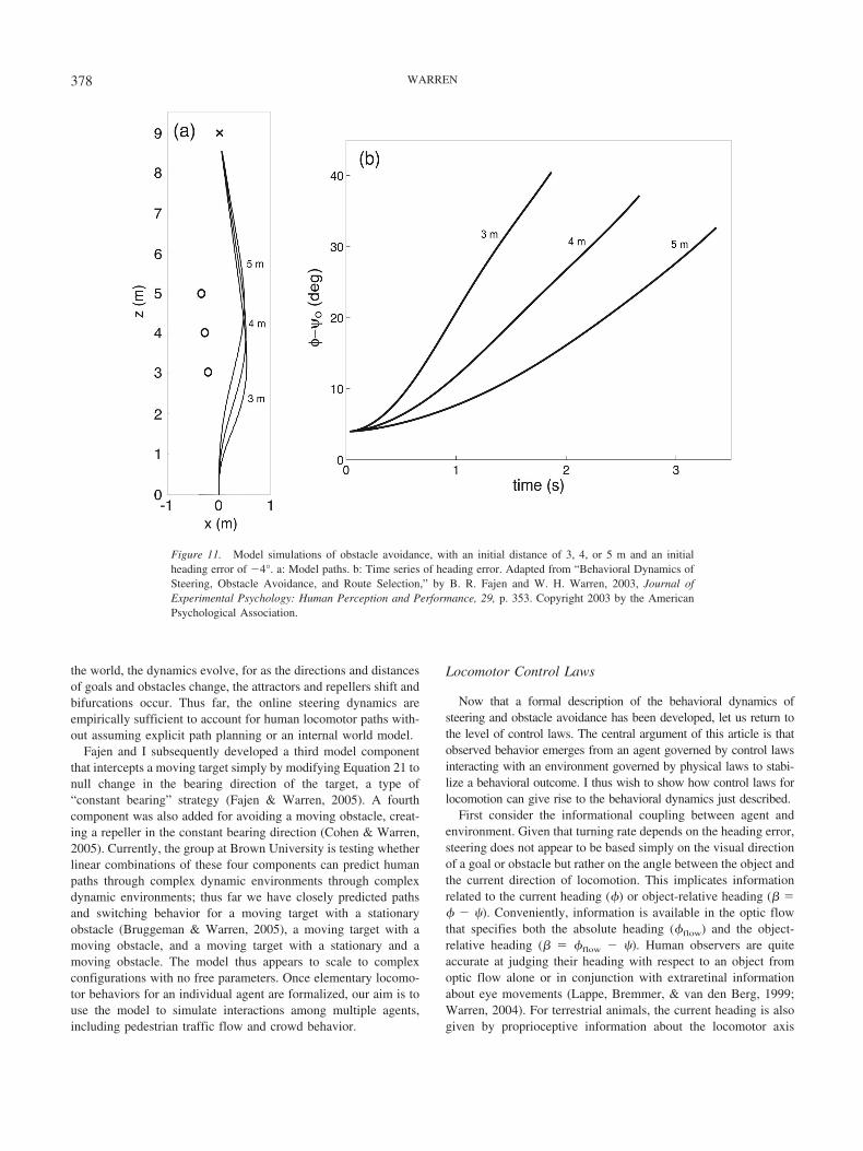
the world, the dynamics evolve, for as the directions and distancesof goals and obstacles change, the attractors and repellers shift andbifurcations occur. Thus far, the online steering dynamics areempirically sufficient to account for human locomotor paths with-out assuming explicit path planning or an internal world model.

Fajen and I subsequently developed a third model componentthat intercepts a moving target simply by modifying Equation 21 tonull change in the bearing direction of the target, a type of“constant bearing” strategy (Fajen & Warren, 2005). A fourthcomponent was also added for avoiding a moving obstacle, creat-ing a repeller in the constant bearing direction (Cohen & Warren,2005). Currently, the group at Brown University is testing whetherlinear combinations of these four components can predict humanpaths through complex dynamic environments through complexdynamic environments; thus far we have closely predicted pathsand switching behavior for a moving target with a stationaryobstacle (Bruggeman & Warren, 2005), a moving target with amoving obstacle, and a moving target with a stationary and amoving obstacle. The model thus appears to scale to complexconfigurations with no free parameters. Once elementary locomo-tor behaviors for an individual agent are formalized, our aim is touse the model to simulate interactions among multiple agents,including pedestrian traffic flow and crowd behavior.

Locomotor Control Laws

Now that a formal description of the behavioral dynamics ofsteering and obstacle avoidance has been developed, let us return tothe level of control laws. The central argument of this article is thatobserved behavior emerges from an agent governed by control lawsinteracting with an environment governed by physical laws to stabi-lize a behavioral outcome. I thus wish to show how control laws forlocomotion can give rise to the behavioral dynamics just described.

First consider the informational coupling between agent andenvironment. Given that turning rate depends on the heading error,steering does not appear to be based simply on the visual directionof a goal or obstacle but rather on the angle between the object andthe current direction of locomotion. This implicates informationrelated to the current heading (�) or object-relative heading (� �� ). Conveniently, information is available in the optic flowthat specifies both the absolute heading (�flow) and the object-relative heading (� � �flow � �). Human observers are quiteaccurate at judging their heading with respect to an object fromoptic flow alone or in conjunction with extraretinal informationabout eye movements (Lappe, Bremmer, & van den Berg, 1999;Warren, 2004). For terrestrial animals, the current heading is alsogiven by proprioceptive information about the locomotor axis

Figure 11. Model simulations of obstacle avoidance, with an initial distance of 3, 4, or 5 m and an initialheading error of �4°. a: Model paths. b: Time series of heading error. Adapted from “Behavioral Dynamics ofSteering, Obstacle Avoidance, and Route Selection,” by B. R. Fajen and W. H. Warren, 2003, Journal ofExperimental Psychology: Human Perception and Performance, 29, p. 353. Copyright 2003 by the AmericanPsychological Association.

378 WARREN

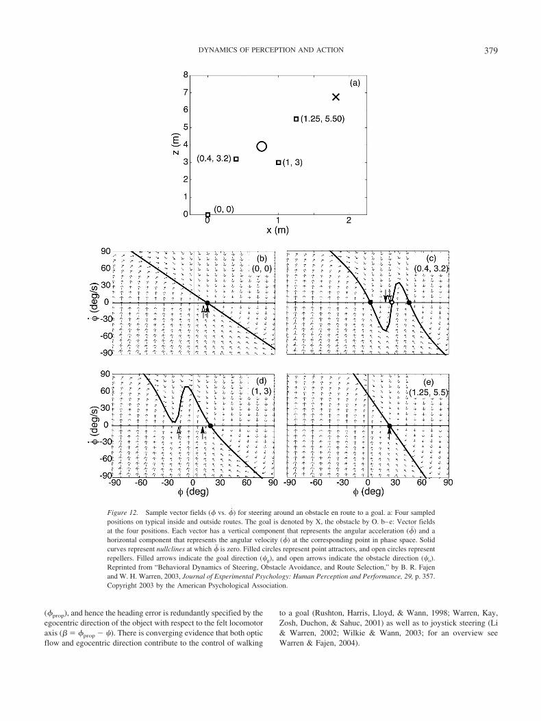
(�prop), and hence the heading error is redundantly specified by theegocentric direction of the object with respect to the felt locomotoraxis (� � �prop � �). There is converging evidence that both opticflow and egocentric direction contribute to the control of walking

to a goal (Rushton, Harris, Lloyd, & Wann, 1998; Warren, Kay,Zosh, Duchon, & Sahuc, 2001) as well as to joystick steering (Li& Warren, 2002; Wilkie & Wann, 2003; for an overview seeWarren & Fajen, 2004).

Figure 12. Sample vector fields (� vs. �) for steering around an obstacle en route to a goal. a: Four sampledpositions on typical inside and outside routes. The goal is denoted by X, the obstacle by O. b–e: Vector fieldsat the four positions. Each vector has a vertical component that represents the angular acceleration (�) and ahorizontal component that represents the angular velocity (�) at the corresponding point in phase space. Solidcurves represent nullclines at which � is zero. Filled circles represent point attractors, and open circles representrepellers. Filled arrows indicate the goal direction (�g), and open arrows indicate the obstacle direction (�o).Reprinted from “Behavioral Dynamics of Steering, Obstacle Avoidance, and Route Selection,” by B. R. Fajenand W. H. Warren, 2003, Journal of Experimental Psychology: Human Perception and Performance, 29, p. 357.Copyright 2003 by the American Psychological Association.


These findings led me and my colleagues to propose a controllaw for steering to a goal (Warren et al., 2001) in which turning isa function of the current heading error given by a linear combi-nation of egocentric direction and optic flow:

� � �kg[(�prop � �g) � wv(�flow � �g)]. (23)

The coefficient kg is a rate constant. The contribution of the flowis weighted by the observer’s velocity v, which influences the flowrate, and by w, a measure of the visual area and magnitude of opticflow due to environmental structure. Thus, as the observer travelsfaster or as there is more visual structure, steering will be increas-ingly dominated by the optic flow, consistent with experimentalevidence (Fink & Warren, 2002; M. G. Harris & Carre, 2001;Warren et al., 2001; Wilkie & Wann, 2002; Wood, Harvey,Young, Beedie, & Wilson, 2000). Conversely, with little visualstructure, the egocentric direction of the target will dominate (J. M.Harris & Bonas, 2002; Rushton, Harris, & Wann, 1999). Suchredundancy is highly adaptive, for it allows locomotor guidance tobe robust under varying environmental conditions.

In the preceding experiments on steering dynamics, it was alsofound that the influence of the goal decays exponentially withdistance (or equivalently, time to contact). The control law canthus be expanded as

�� kg[(�prop � �g) � wv(�flow � �g)](e�c1dg � c2).

(24)

This control law is represented as a first-order dynamical systemthat relaxes to an attractor for the intended heading in a direction�� with a relaxation rate ��. The prime indicates that the intendedheading is a control variable, and its relaxation rate is distinct froma physical turning rate. In principle, the equation can be expandedfurther by adding the obstacle term:

�� kg[(�prop � �g) � wv(�flow � �g)](e�c1dg � c2)

� ko[(�prop � �g) � wv(�flow � �g)](e�c3��o�)(e�c4do). (25)

The system relaxes to a heading that is determined by the currentconfiguration of goals and obstacles. This control law thus mapslow-dimensional informational variables that specify heading errorinto a low-dimensional control variable for the intended heading.The control law is what the agent’s perceptual–motor system mustlearn, including the form of the first-order function (which is thesame for each component), the relaxation rates kg and ko, thespread of the obstacle repulsion function (which reflects theagent’s body size), and the decay rates for obstacles and goals withdistance.

Next consider the mechanical coupling between agent and en-vironment. Given an intended heading direction, the locomotorsystem transforms this control variable into forces exerted in theenvironment. Effectively, this means changing the direction ofmotion of the body’s center of mass and simultaneously rotatingthe trunk via forces applied through the supporting foot against theground (Patla, Adkin, & Ballard, 1999). Reaction forces produce achange in the direction of travel in accordance with the laws ofphysics. Given that the physical body is an inertial system, it mustundergo angular acceleration and will necessarily lag behind the

intended heading. Body motion can thus be represented as alumped second-order system,

� � �bb� � kb(� � ��), (26)

where the mass term is incorporated in the parameters as before,and the parameter values are fixed. The damping parameter isinterpreted as a physical constraint related to centripetal force andthus need not be learned. The observed angular acceleration is thusa function of the discrepancy between the current and intendedheading (� � ��). Finally, the resulting change in heading altersthe information available at the moving eye in accordance with thelaws of ecological optics, resulting in a shift of the optic flow aswell as the visual directions of goals and obstacles.

It is now possible to see how the behavioral dynamics emergefrom the interaction between an agent governed by control lawsand an environment governed by physical laws. As described inFajen and Warren (2003), Philip Fink simulated this perception–action cycle for steering around an obstacle to a goal, by embed-ding the first-order control law (Equation 22) within a second-order body (Equation 23). The resulting paths wereindistinguishable from those generated by the model of the behav-ioral dynamics (Equation 19). Moreover, the time series of headingerror fit the mean human data and accounted for a proportion of.991 of the variance (parameter values kg � 59.1625, c1 � .0555,c2 � .01125, ko � 842, c3 � 2.74063, c4 � .04653, bb � .0375,kb � 592).12 This result demonstrates formally how theperception–action cycle gives rise to the behavioral dynamics.

Bootstrapping Adaptive Behavior

We are now in a position to consider how such adaptive behav-ior patterns might come about. The aim is to show how stablebehavior could arise through a process of self-organization,thereby circumventing an appeal to a priori internal organization.Such pattern formation processes typically occur in physical sys-tems with many simple interacting components (Haken, 1977;Nicolis & Prigogine, 1989), but they also occur in biologicalsystems with more complex components that are coupled togetherby sensory information (Camazine et al., 2001; Murray, 1989;Yates, 1987). I wish to extend such an analysis to the interactionsbetween a complex individual and a complex environment undercertain physical and informational constraints.

Self-organization is the spontaneous formation of ordered statesin complex systems under specific boundary conditions. First, it istypically observed in open systems composed of many individualcomponents with many degrees of freedom. Second, the compo-nents must be coupled together so that they are interacting locallyand simultaneously. Third, the presence of fluctuations or insta-bilities produces a symmetry-breaking event, which launches thepattern-formation process. Most important, there must be a non-linear positive feedback that amplifies the initial instability, so thatthe emerging pattern feeds back to capture the behavior of indi-vidual components. In effect, this acts to compress or enslave the

12 These parameter values are different from those for the behavioraldynamics because they reflect the relaxation rate for a first-order controllaw, which is embedded in a second-order physical system.

380 WARREN

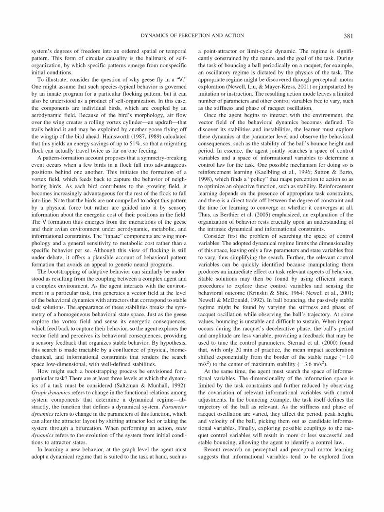
system’s degrees of freedom into an ordered spatial or temporalpattern. This form of circular causality is the hallmark of self-organization, by which specific patterns emerge from nonspecificinitial conditions.

To illustrate, consider the question of why geese fly in a “V.”One might assume that such species-typical behavior is governedby an innate program for a particular flocking pattern, but it canalso be understood as a product of self-organization. In this case,the components are individual birds, which are coupled by anaerodynamic field. Because of the bird’s morphology, air flowover the wing creates a rolling vortex cylinder—an updraft—thattrails behind it and may be exploited by another goose flying offthe wingtip of the bird ahead. Hainsworth (1987, 1989) calculatedthat this yields an energy savings of up to 51%, so that a migratingflock can actually travel twice as far on one feeding.

A pattern-formation account proposes that a symmetry-breakingevent occurs when a few birds in a flock fall into advantageouspositions behind one another. This initiates the formation of avortex field, which feeds back to capture the behavior of neigh-boring birds. As each bird contributes to the growing field, itbecomes increasingly advantageous for the rest of the flock to fallinto line. Note that the birds are not compelled to adopt this patternby a physical force but rather are guided into it by sensoryinformation about the energetic cost of their positions in the field.The V formation thus emerges from the interactions of the geeseand their avian environment under aerodynamic, metabolic, andinformational constraints. The “innate” components are wing mor-phology and a general sensitivity to metabolic cost rather than aspecific behavior per se. Although this view of flocking is stillunder debate, it offers a plausible account of behavioral patternformation that avoids an appeal to genetic neural programs.

The bootstrapping of adaptive behavior can similarly be under-stood as resulting from the coupling between a complex agent anda complex environment. As the agent interacts with the environ-ment in a particular task, this generates a vector field at the levelof the behavioral dynamics with attractors that correspond to stabletask solutions. The appearance of these stabilities breaks the sym-metry of a homogeneous behavioral state space. Just as the geeseexplore the vortex field and sense its energetic consequences,which feed back to capture their behavior, so the agent explores thevector field and perceives its behavioral consequences, providinga sensory feedback that organizes stable behavior. By hypothesis,this search is made tractable by a confluence of physical, biome-chanical, and informational constraints that renders the searchspace low-dimensional, with well-defined stabilities.

How might such a bootstrapping process be envisioned for aparticular task? There are at least three levels at which the dynam-ics of a task must be considered (Saltzman & Munhall, 1992).Graph dynamics refers to change in the functional relations amongsystem components that determine a dynamical regime—ab-stractly, the function that defines a dynamical system. Parameterdynamics refers to change in the parameters of this function, whichcan alter the attractor layout by shifting attractor loci or taking thesystem through a bifurcation. When performing an action, statedynamics refers to the evolution of the system from initial condi-tions to attractor states.

In learning a new behavior, at the graph level the agent mustadopt a dynamical regime that is suited to the task at hand, such as

a point-attractor or limit-cycle dynamic. The regime is signifi-cantly constrained by the nature and the goal of the task. Duringthe task of bouncing a ball periodically on a racquet, for example,an oscillatory regime is dictated by the physics of the task. Theappropriate regime might be discovered through perceptual–motorexploration (Newell, Liu, & Mayer-Kress, 2001) or jumpstarted byimitation or instruction. The resulting action mode leaves a limitednumber of parameters and other control variables free to vary, suchas the stiffness and phase of racquet oscillation.

Once the agent begins to interact with the environment, thevector field of the behavioral dynamics becomes defined. Todiscover its stabilities and instabilities, the learner must explorethese dynamics at the parameter level and observe the behavioralconsequences, such as the stability of the ball’s bounce height andperiod. In essence, the agent jointly searches a space of controlvariables and a space of informational variables to determine acontrol law for the task. One possible mechanism for doing so isreinforcement learning (Kaelbling et al., 1996; Sutton & Barto,1998), which finds a “policy” that maps perception to action so asto optimize an objective function, such as stability. Reinforcementlearning depends on the presence of appropriate task constraints,and there is a direct trade-off between the degree of constraint andthe time for learning to converge or whether it converges at all.Thus, as Berthier et al. (2005) emphasized, an explanation of theorganization of behavior rests crucially upon an understanding ofthe intrinsic dynamical and informational constraints.

Consider first the problem of searching the space of controlvariables. The adopted dynamical regime limits the dimensionalityof this space, leaving only a few parameters and state variables freeto vary, thus simplifying the search. Further, the relevant controlvariables can be quickly identified because manipulating themproduces an immediate effect on task-relevant aspects of behavior.Stable solutions may then be found by using efficient searchprocedures to explore these control variables and sensing thebehavioral outcome (Krinskii & Shik, 1964; Newell et al., 2001;Newell & McDonald, 1992). In ball bouncing, the passively stableregime might be found by varying the stiffness and phase ofracquet oscillation while observing the ball’s trajectory. At somevalues, bouncing is unstable and difficult to sustain. When impactoccurs during the racquet’s decelerative phase, the ball’s periodand amplitude are less variable, providing a feedback that may beused to tune the control parameters. Sternad et al. (2000) foundthat, with only 20 min of practice, the mean impact accelerationshifted exponentially from the border of the stable range (�1.0m/s2) to the center of maximum stability (�3.6 m/s2).

At the same time, the agent must search the space of informa-tional variables. The dimensionality of the information space islimited by the task constraints and further reduced by observingthe covariation of relevant informational variables with controladjustments. In the bouncing example, the task itself defines thetrajectory of the ball as relevant. As the stiffness and phase ofracquet oscillation are varied, they affect the period, peak height,and velocity of the ball, picking them out as candidate informa-tional variables. Finally, exploring possible couplings to the rac-quet control variables will result in more or less successful andstable bouncing, allowing the agent to identify a control law.

Recent research on perceptual and perceptual–motor learningsuggests that informational variables tend to be explored from


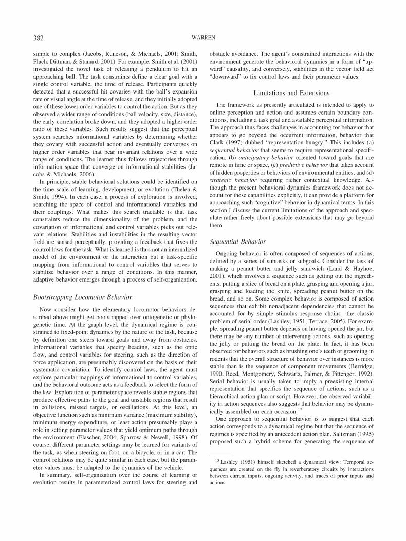
simple to complex (Jacobs, Runeson, & Michaels, 2001; Smith,Flach, Dittman, & Stanard, 2001). For example, Smith et al. (2001)investigated the novel task of releasing a pendulum to hit anapproaching ball. The task constraints define a clear goal with asingle control variable, the time of release. Participants quicklydetected that a successful hit covaries with the ball’s expansionrate or visual angle at the time of release, and they initially adoptedone of these lower order variables to control the action. But as theyobserved a wider range of conditions (ball velocity, size, distance),the early correlation broke down, and they adopted a higher orderratio of these variables. Such results suggest that the perceptualsystem searches informational variables by determining whetherthey covary with successful action and eventually converges onhigher order variables that bear invariant relations over a widerange of conditions. The learner thus follows trajectories throughinformation space that converge on informational stabilities (Ja-cobs & Michaels, 2006).

In principle, stable behavioral solutions could be identified onthe time scale of learning, development, or evolution (Thelen &Smith, 1994). In each case, a process of exploration is involved,searching the space of control and informational variables andtheir couplings. What makes this search tractable is that taskconstraints reduce the dimensionality of the problem, and thecovariation of informational and control variables picks out rele-vant relations. Stabilities and instabilities in the resulting vectorfield are sensed perceptually, providing a feedback that fixes thecontrol laws for the task. What is learned is thus not an internalizedmodel of the environment or the interaction but a task-specificmapping from informational to control variables that serves tostabilize behavior over a range of conditions. In this manner,adaptive behavior emerges through a process of self-organization.

Bootstrapping Locomotor Behavior

Now consider how the elementary locomotor behaviors de-scribed above might get bootstrapped over ontogenetic or phylo-genetic time. At the graph level, the dynamical regime is con-strained to fixed-point dynamics by the nature of the task, becauseby definition one steers toward goals and away from obstacles.Informational variables that specify heading, such as the opticflow, and control variables for steering, such as the direction offorce application, are presumably discovered on the basis of theirsystematic covariation. To identify control laws, the agent mustexplore particular mappings of informational to control variables,and the behavioral outcome acts as a feedback to select the form ofthe law. Exploration of parameter space reveals stable regions thatproduce effective paths to the goal and unstable regions that resultin collisions, missed targets, or oscillations. At this level, anobjective function such as minimum variance (maximum stability),minimum energy expenditure, or least action presumably plays arole in setting parameter values that yield optimum paths throughthe environment (Flascher, 2004; Sparrow & Newell, 1998). Ofcourse, different parameter settings may be learned for variants ofthe task, as when steering on foot, on a bicycle, or in a car: Thecontrol relations may be quite similar in each case, but the param-eter values must be adapted to the dynamics of the vehicle.

In summary, self-organization over the course of learning orevolution results in parameterized control laws for steering and

obstacle avoidance. The agent’s constrained interactions with theenvironment generate the behavioral dynamics in a form of “up-ward” causality, and conversely, stabilities in the vector field act“downward” to fix control laws and their parameter values.

Limitations and Extensions

The framework as presently articulated is intended to apply toonline perception and action and assumes certain boundary con-ditions, including a task goal and available perceptual information.The approach thus faces challenges in accounting for behavior thatappears to go beyond the occurrent information, behavior thatClark (1997) dubbed “representation-hungry.” This includes (a)sequential behavior that seems to require representational specifi-cation, (b) anticipatory behavior oriented toward goals that areremote in time or space, (c) predictive behavior that takes accountof hidden properties or behaviors of environmental entities, and (d)strategic behavior requiring richer contextual knowledge. Al-though the present behavioral dynamics framework does not ac-count for these capabilities explicitly, it can provide a platform forapproaching such “cognitive” behavior in dynamical terms. In thissection I discuss the current limitations of the approach and spec-ulate rather freely about possible extensions that may go beyondthem.

Sequential Behavior

Ongoing behavior is often composed of sequences of actions,defined by a series of subtasks or subgoals. Consider the task ofmaking a peanut butter and jelly sandwich (Land & Hayhoe,2001), which involves a sequence such as getting out the ingredi-ents, putting a slice of bread on a plate, grasping and opening a jar,grasping and loading the knife, spreading peanut butter on thebread, and so on. Some complex behavior is composed of actionsequences that exhibit nonadjacent dependencies that cannot beaccounted for by simple stimulus–response chains—the classicproblem of serial order (Lashley, 1951; Terrace, 2005). For exam-ple, spreading peanut butter depends on having opened the jar, butthere may be any number of intervening actions, such as openingthe jelly or putting the bread on the plate. In fact, it has beenobserved for behaviors such as brushing one’s teeth or grooming inrodents that the overall structure of behavior over instances is morestable than is the sequence of component movements (Berridge,1990; Reed, Montgomery, Schwartz, Palmer, & Pittenger, 1992).Serial behavior is usually taken to imply a preexisting internalrepresentation that specifies the sequence of actions, such as ahierarchical action plan or script. However, the observed variabil-ity in action sequences also suggests that behavior may be dynam-ically assembled on each occasion.13

One approach to sequential behavior is to suggest that eachaction corresponds to a dynamical regime but that the sequence ofregimes is specified by an antecedent action plan. Saltzman (1995)proposed such a hybrid scheme for generating the sequence of

13 Lashley (1951) himself sketched a dynamical view: Temporal se-quences are created on the fly in reverberatory circuits by interactionsbetween current inputs, ongoing activity, and traces of prior inputs andactions.

382 WARREN

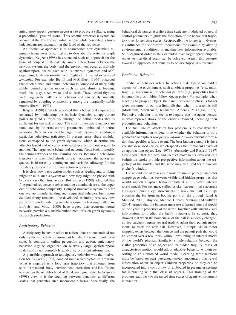
articulatory speech gestures necessary to produce a syllable, usinga predefined “gestural score.” This scheme preserves a dynamicalaccount at the level of individual actions while conceding a time-independent representation at the level of the sequence.

An alternative approach is to characterize how dynamical re-gimes change over time, that is, to describe the system’s graphdynamics. Keijzer (1998) has sketched such an approach on thebasis of coupled multiscale dynamics. Interactions between thenervous system, the body, and the environment occur at multiplespatiotemporal scales, each with its intrinsic dynamics and self-organizing tendencies—what one might call a nested behavioraldynamics. For example, Iberall and McCulloch (1969) observedthat much human and animal behavior is composed of marginallystable, periodic action modes such as gait, drinking, feeding,work–rest, play, sleep–wake, and so forth. These nested rhythmsyield large-scale patterns of behavior and can be dynamicallyregulated by coupling or switching among the marginally stablemodes (Iberall, 1977).

Keijzer (1998) similarly proposed that a behavioral sequence isgenerated by modulating the intrinsic dynamics at appropriatepoints to yield a trajectory through the action modes that issufficient for the task at hand. The short time-scale dynamics aremodulated by “internal control parameters” embodied in neuralnetworks; they are coupled to larger scale dynamics, yielding aparticular behavioral trajectory. In present terms, these modula-tions correspond to the graph dynamics, which determine theattractor layout and when the system bifurcates from one regime toanother. The large-scale behavioral outcome feeds back to modifythe neural networks so that learning occurs. Because a behavioraltrajectory is assembled afresh on each occasion, the action se-quence is historically contingent and variable, allowing for theflexibility observed in ordinary action sequences.

It is clear how basic action modes such as feeding and drinkingmight arise in such a system and how they might be phased withbehavior on other time scales. But Keijzer (1998) admitted thatfine-grained sequences such as making a sandwich are at the upperend of behavioral complexity. Coupled multiscale dynamics offerone avenue to understanding such sequential behavior, but a moredetailed theory remains to be developed, including precisely howpatterns of mode switching may be acquired in learning. Saltzman,Lofqvist, and Mitra (2000) have argued that recurrent neuralnetworks provide a plausible embodiment of such graph dynamicsin speech production.

Anticipatory Behavior

Anticipatory behavior refers to actions that are constrained notonly by the immediate environment but also by some remote goalstate. In contrast to online perception and action, anticipatorybehavior may be organized on relatively large spatiotemporalscales and is not completely guided by occurrent information.

A plausible approach to anticipatory behavior was the motiva-tion for Keijzer’s (1998) coupled multiscaled dynamics program.What is required is a long-term trajectory that emerges fromshort-term neural–body–environment interactions and is sufficientto arrive in the neighborhood of the desired goal state. In Keijzer’s(1998) view, it is the coupling between dynamics at differentscales that generates such macroscopic forms. Specifically, the

behavioral dynamics at a short time scale are modulated by neuralcontrol parameters to guide the formation of the behavioral trajec-tory over longer time scales. Reciprocally, the longer term dynam-ics influence the short-term interactions, for example by alteringenvironmental conditions or making new information available.Self-organized order is thus extended over larger spatiotemporalscales so that distal goals can be achieved. Again, this gesturestoward an approach that remains to be developed in substance.

Predictive Behavior

Predictive behavior refers to actions that depend on hiddenaspects of the environment, such as object properties (e.g., mass,fragility, slipperiness) or behavior patterns (e.g., projectiles travelin parabolic arcs, rabbits follow zigzag paths). For example, whenreaching to grasp an object, the hand deceleration phase is longerwhen the target object is a lightbulb than when it is a tennis ball(Marteniuk, MacKenzie, Jeannerod, Athenes, & Dugas, 1987).Predictive behavior thus seems to require that the agent possessinternal representations of the entities involved, including theirproperties and behaviors.

The first line of attack on this problem is to reanalyze theavailable information to determine whether the behavior is trulypredictive or exploits prospective information—occurrent informa-tion that specifies a future event. The best-known example is the

variable described earlier, which specifies the immanent arrival ofan approaching object (Lee, 1976). Abernathy and Russell (1987)have shown that the arm and racquet movements involved in abadminton stroke provide prospective information about the tra-jectory of the shuttle, and the same may also hold for a baseballpitcher’s windup.

The second line of attack is to look for simple perceptual–motormappings or relations between visible and hidden properties thatwould support adaptive behavior without a full-blown internalworld model. For instance, skilled cricket batsmen make accuratehigh-speed pursuit eye movements to track the ball as it ap-proaches the bat from its bounce point on the ground (Land &McLeod, 2000). Hayhoe, Mennie, Gorgos, Semrau, and Sullivan(2004) argued that the batsmen must use a learned internal modelof the dynamic properties of the world, together with current visualinformation, to predict the ball’s trajectory. In support, theyshowed that when the bounciness of the ball is suddenly changed,novice catchers require several trials to adapt their pursuit move-ments to track the new ball. However, a simple visual–motormapping exists between the bounce and the pursuit path that couldbe learned over a few trials, without presuming an internal modelof the world’s physics. Similarly, simple relations between thevisible properties of an object and its hidden fragility, mass, orcharacteristic motion would allow adaptive behavior without re-sorting to an elaborated world model. Learning these relationsmust be based on past perceptual–motor encounters that revealinformation about an object’s hidden properties, so they can beincorporated into a control law or embodied in parameter settingsfor interacting with that class of objects. This framing of theproblem leads back to the nested time scales of agent–environmentinteraction.


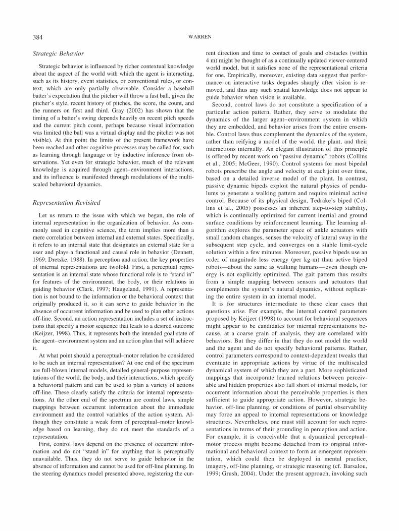
Strategic Behavior

Strategic behavior is influenced by richer contextual knowledgeabout the aspect of the world with which the agent is interacting,such as its history, event statistics, or conventional rules, or con-text, which are only partially observable. Consider a baseballbatter’s expectation that the pitcher will throw a fast ball, given thepitcher’s style, recent history of pitches, the score, the count, andthe runners on first and third. Gray (2002) has shown that thetiming of a batter’s swing depends heavily on recent pitch speedsand the current pitch count, perhaps because visual informationwas limited (the ball was a virtual display and the pitcher was notvisible). At this point the limits of the present framework havebeen reached and other cognitive processes may be called for, suchas learning through language or by inductive inference from ob-servations. Yet even for strategic behavior, much of the relevantknowledge is acquired through agent–environment interactions,and its influence is manifested through modulations of the multi-scaled behavioral dynamics.

Representation Revisited

Let us return to the issue with which we began, the role ofinternal representation in the organization of behavior. As com-monly used in cognitive science, the term implies more than amere correlation between internal and external states. Specifically,it refers to an internal state that designates an external state for auser and plays a functional and causal role in behavior (Dennett,1969; Dretske, 1988). In perception and action, the key propertiesof internal representations are twofold. First, a perceptual repre-sentation is an internal state whose functional role is to “stand in”for features of the environment, the body, or their relations inguiding behavior (Clark, 1997; Haugeland, 1991). A representa-tion is not bound to the information or the behavioral context thatoriginally produced it, so it can serve to guide behavior in theabsence of occurrent information and be used to plan other actionsoff-line. Second, an action representation includes a set of instruc-tions that specify a motor sequence that leads to a desired outcome(Keijzer, 1998). Thus, it represents both the intended goal state ofthe agent–environment system and an action plan that will achieveit.

At what point should a perceptual–motor relation be consideredto be such an internal representation? At one end of the spectrumare full-blown internal models, detailed general-purpose represen-tations of the world, the body, and their interactions, which specifya behavioral pattern and can be used to plan a variety of actionsoff-line. These clearly satisfy the criteria for internal representa-tions. At the other end of the spectrum are control laws, simplemappings between occurrent information about the immediateenvironment and the control variables of the action system. Al-though they constitute a weak form of perceptual–motor knowl-edge based on learning, they do not meet the standards of arepresentation.

First, control laws depend on the presence of occurrent infor-mation and do not “stand in” for anything that is perceptuallyunavailable. Thus, they do not serve to guide behavior in theabsence of information and cannot be used for off-line planning. Inthe steering dynamics model presented above, registering the cur-

rent direction and time to contact of goals and obstacles (within4 m) might be thought of as a continually updated viewer-centeredworld model, but it satisfies none of the representational criteriafor one. Empirically, moreover, existing data suggest that perfor-mance on interactive tasks degrades sharply after vision is re-moved, and thus any such spatial knowledge does not appear toguide behavior when vision is available.

Second, control laws do not constitute a specification of aparticular action pattern. Rather, they serve to modulate thedynamics of the larger agent– environment system in whichthey are embedded, and behavior arises from the entire ensem-ble. Control laws thus complement the dynamics of the system,rather than reifying a model of the world, the plant, and theirinteractions internally. An elegant illustration of this principleis offered by recent work on “passive dynamic” robots (Collinset al., 2005; McGeer, 1990). Control systems for most bipedalrobots prescribe the angle and velocity at each joint over time,based on a detailed inverse model of the plant. In contrast,passive dynamic bipeds exploit the natural physics of pendu-lums to generate a walking pattern and require minimal activecontrol. Because of its physical design, Tedrake’s biped (Col-lins et al., 2005) possesses an inherent step-to-step stability,which is continually optimized for current inertial and groundsurface conditions by reinforcement learning. The learning al-gorithm explores the parameter space of ankle actuators withsmall random changes, senses the velocity of lateral sway in thesubsequent step cycle, and converges on a stable limit-cyclesolution within a few minutes. Moreover, passive bipeds use anorder of magnitude less energy (per kg-m) than active bipedrobots—about the same as walking humans— even though en-ergy is not explicitly optimized. The gait pattern thus resultsfrom a simple mapping between sensors and actuators thatcomplements the system’s natural dynamics, without replicat-ing the entire system in an internal model.

It is for structures intermediate to these clear cases thatquestions arise. For example, the internal control parametersproposed by Keijzer (1998) to account for behavioral sequencesmight appear to be candidates for internal representations be-cause, at a coarse grain of analysis, they are correlated withbehaviors. But they differ in that they do not model the worldand the agent and do not specify behavioral patterns. Rather,control parameters correspond to context-dependent tweaks thateventuate in appropriate actions by virtue of the multiscaleddynamical system of which they are a part. More sophisticatedmappings that incorporate learned relations between perceiv-able and hidden properties also fall short of internal models, foroccurrent information about the perceivable properties is thensufficient to guide appropriate action. However, strategic be-havior, off-line planning, or conditions of partial observabilitymay force an appeal to internal representations or knowledgestructures. Nevertheless, one must still account for such repre-sentations in terms of their grounding in perception and action.For example, it is conceivable that a dynamical perceptual–motor process might become detached from its original infor-mational and behavioral context to form an emergent represen-tation, which could then be deployed in mental practice,imagery, off-line planning, or strategic reasoning (cf. Barsalou,1999; Grush, 2004). Under the present approach, invoking such

384 WARREN

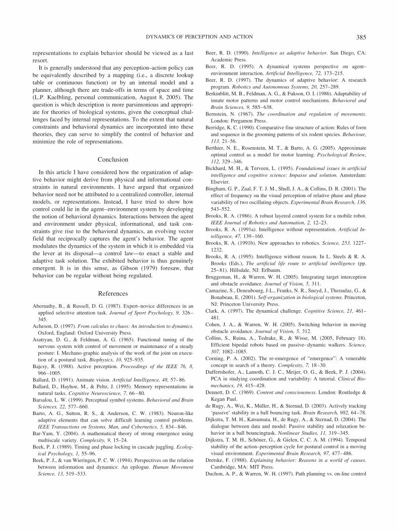
representations to explain behavior should be viewed as a lastresort.

It is generally understood that any perception–action policy canbe equivalently described by a mapping (i.e., a discrete lookuptable or continuous function) or by an internal model and aplanner, although there are trade-offs in terms of space and time(L.P. Kaelbling, personal communication, August 8, 2005). Thequestion is which description is more parsimonious and appropri-ate for theories of biological systems, given the conceptual chal-lenges faced by internal representations. To the extent that naturalconstraints and behavioral dynamics are incorporated into thesetheories, they can serve to simplify the control of behavior andminimize the role of representations.

Conclusion

In this article I have considered how the organization of adap-tive behavior might derive from physical and informational con-straints in natural environments. I have argued that organizedbehavior need not be attributed to a centralized controller, internalmodels, or representations. Instead, I have tried to show howcontrol could lie in the agent–environment system by developingthe notion of behavioral dynamics. Interactions between the agentand environment under physical, informational, and task con-straints give rise to the behavioral dynamics, an evolving vectorfield that reciprocally captures the agent’s behavior. The agentmodulates the dynamics of the system in which it is embedded viathe lever at its disposal—a control law—to enact a stable andadaptive task solution. The exhibited behavior is thus genuinelyemergent. It is in this sense, as Gibson (1979) foresaw, thatbehavior can be regular without being regulated.

References

Abernathy, B., & Russell, D. G. (1987). Expert–novice differences in anapplied selective attention task. Journal of Sport Psychology, 9, 326–345.

Acheson, D. (1997). From calculus to chaos: An introduction to dynamics.Oxford, England: Oxford University Press.

Asatryan, D. G., & Feldman, A. G. (1965). Functional tuning of thenervous system with control of movement or maintenance of a steadyposture: I. Mechano-graphic analysis of the work of the joint on execu-tion of a postural task. Biophysics, 10, 925–935.

Bajcsy, R. (1988). Active perception. Proceedings of the IEEE 76, 8,966–1005.

Ballard, D. (1991). Animate vision. Artificial Intelligence, 48, 57–86.Ballard, D., Hayhoe, M., & Peltz, J. (1995). Memory representations in

natural tasks. Cognitive Neuroscience, 7, 66–80.Barsalou, L. W. (1999). Perceptual symbol systems. Behavioral and Brain

Sciences, 22, 577–660.Barto, A. G., Sutton, R. S., & Anderson, C. W. (1983). Neuron-like

adaptive elements that can solve difficult learning control problems.IEEE Transactions on Systems, Man, and Cybernetics, 5, 834–846.

Bar-Yam, Y. (2004). A mathematical theory of strong emergence usingmultiscale variety. Complexity, 9, 15–24.

Beek, P. J. (1989). Timing and phase locking in cascade juggling. Ecolog-ical Psychology, 1, 55–96.

Beek, P. J., & van Wieringen, P. C. W. (1994). Perspectives on the relationbetween information and dynamics: An epilogue. Human MovementScience, 13, 519–533.

Beer, R. D. (1990). Intelligence as adaptive behavior. San Diego, CA:Academic Press.

Beer, R. D. (1995). A dynamical systems perspective on agent–environment interaction. Artificial Intelligence, 72, 173–215.

Beer, R. D. (1997). The dynamics of adaptive behavior: A researchprogram. Robotics and Autonomous Systems, 20, 257–289.

Berkinblitt, M. B., Feldman, A. G., & Fukson, O. I. (1986). Adaptability ofinnate motor patterns and motor control mechanisms. Behavioral andBrain Sciences, 9, 585–638.

Bernstein, N. (1967). The coordination and regulation of movements.London: Pergamon Press.

Berridge, K. C. (1990). Comparative fine structure of action: Rules of formand sequence in the grooming patterns of six rodent species. Behaviour,113, 21–56.

Berthier, N. E., Rosenstein, M. T., & Barto, A. G. (2005). Approximateoptimal control as a model for motor learning. Psychological Review,112, 329–346.

Bickhard, M. H., & Terveen, L. (1995). Foundational issues in artificialintelligence and cognitive science: Impasse and solution. Amsterdam:Elsevier.

Bingham, G. P., Zaal, F. T. J. M., Shull, J. A., & Collins, D. R. (2001). Theeffect of frequency on the visual perception of relative phase and phasevariability of two oscillating objects. Experimental Brain Research, 136,543–552.

Brooks, R. A. (1986). A robust layered control system for a mobile robot.IEEE Journal of Robotics and Automation, 2, 12–23.

Brooks, R. A. (1991a). Intelligence without representation. Artificial In-telligence, 47, 139–160.

Brooks, R. A. (1991b). New approaches to robotics. Science, 253, 1227–1232.

Brooks, R. A. (1995). Intelligence without reason. In L. Steels & R. A.Brooks (Eds.), The artificial life route to artificial intelligence (pp.25–81). Hillsdale, NJ: Erlbaum.

Bruggeman, H., & Warren, W. H. (2005). Integrating target interceptionand obstacle avoidance. Journal of Vision, 5, 311.

Camazine, S., Deneubourg, J-L., Franks, N. R., Sneyd, J., Theraulaz, G., &Bonabeau, E. (2001). Self-organization in biological systems. Princeton,NJ: Princeton University Press.

Clark, A. (1997). The dynamical challenge. Cognitive Science, 21, 461–481.

Cohen, J. A., & Warren, W. H. (2005). Switching behavior in movingobstacle avoidance. Journal of Vision, 5, 312.

Collins, S., Ruina, A., Tedrake, R., & Wisse, M. (2005, February 18).Efficient bipedal robots based on passive–dynamic walkers. Science,307, 1082–1085.

Corning, P. A. (2002). The re-emergence of “emergence”: A venerableconcept in search of a theory. Complexity, 7, 18–30.

Daffertshofer, A., Lamoth, C. J. C., Meijer, O. G., & Beek, P. J. (2004).PCA in studying coordination and variability: A tutorial. Clinical Bio-mechanics, 19, 415–428.

Dennett, D. C. (1969). Content and consciousness. London: Routledge &Kegan Paul.

de Rugy, A., Wei, K., Muller, H., & Sternad, D. (2003). Actively tracking‘passive’ stability in a ball bouncing task. Brain Research, 982, 64–78.

Dijkstra, T. M. H., Katsumata, H., de Rugy, A., & Sternad, D. (2004). Thedialogue between data and model: Passive stability and relaxation be-havior in a ball bouncingtask. Nonlinear Studies, 11, 319–345.

Dijkstra, T. M. H., Schoner, G., & Gielen, C. C. A. M. (1994). Temporalstability of the action–perception cycle for postural control in a movingvisual environment. Experimental Brain Research, 97, 477–486.

Dretske, F. (1988). Explaining behavior: Reasons in a world of causes.Cambridge, MA: MIT Press.

Duchon, A. P., & Warren, W. H. (1997). Path planning vs. on-line control


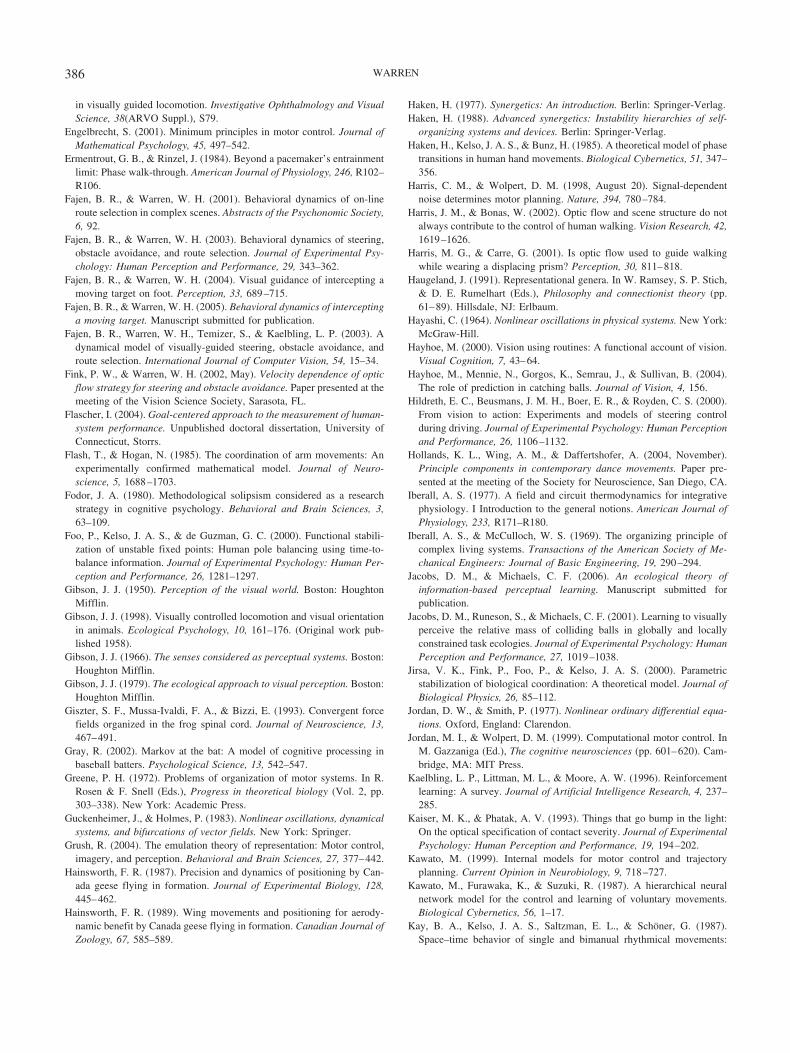
in visually guided locomotion. Investigative Ophthalmology and VisualScience, 38(ARVO Suppl.), S79.

Engelbrecht, S. (2001). Minimum principles in motor control. Journal ofMathematical Psychology, 45, 497–542.

Ermentrout, G. B., & Rinzel, J. (1984). Beyond a pacemaker’s entrainmentlimit: Phase walk-through. American Journal of Physiology, 246, R102–R106.

Fajen, B. R., & Warren, W. H. (2001). Behavioral dynamics of on-lineroute selection in complex scenes. Abstracts of the Psychonomic Society,6, 92.

Fajen, B. R., & Warren, W. H. (2003). Behavioral dynamics of steering,obstacle avoidance, and route selection. Journal of Experimental Psy-chology: Human Perception and Performance, 29, 343–362.

Fajen, B. R., & Warren, W. H. (2004). Visual guidance of intercepting amoving target on foot. Perception, 33, 689–715.

Fajen, B. R., & Warren, W. H. (2005). Behavioral dynamics of interceptinga moving target. Manuscript submitted for publication.

Fajen, B. R., Warren, W. H., Temizer, S., & Kaelbling, L. P. (2003). Adynamical model of visually-guided steering, obstacle avoidance, androute selection. International Journal of Computer Vision, 54, 15–34.

Fink, P. W., & Warren, W. H. (2002, May). Velocity dependence of opticflow strategy for steering and obstacle avoidance. Paper presented at themeeting of the Vision Science Society, Sarasota, FL.

Flascher, I. (2004). Goal-centered approach to the measurement of human-system performance. Unpublished doctoral dissertation, University ofConnecticut, Storrs.

Flash, T., & Hogan, N. (1985). The coordination of arm movements: Anexperimentally confirmed mathematical model. Journal of Neuro-science, 5, 1688–1703.

Fodor, J. A. (1980). Methodological solipsism considered as a researchstrategy in cognitive psychology. Behavioral and Brain Sciences, 3,63–109.

Foo, P., Kelso, J. A. S., & de Guzman, G. C. (2000). Functional stabili-zation of unstable fixed points: Human pole balancing using time-to-balance information. Journal of Experimental Psychology: Human Per-ception and Performance, 26, 1281–1297.

Gibson, J. J. (1950). Perception of the visual world. Boston: HoughtonMifflin.

Gibson, J. J. (1998). Visually controlled locomotion and visual orientationin animals. Ecological Psychology, 10, 161–176. (Original work pub-lished 1958).

Gibson, J. J. (1966). The senses considered as perceptual systems. Boston:Houghton Mifflin.

Gibson, J. J. (1979). The ecological approach to visual perception. Boston:Houghton Mifflin.

Giszter, S. F., Mussa-Ivaldi, F. A., & Bizzi, E. (1993). Convergent forcefields organized in the frog spinal cord. Journal of Neuroscience, 13,467–491.

Gray, R. (2002). Markov at the bat: A model of cognitive processing inbaseball batters. Psychological Science, 13, 542–547.

Greene, P. H. (1972). Problems of organization of motor systems. In R.Rosen & F. Snell (Eds.), Progress in theoretical biology (Vol. 2, pp.303–338). New York: Academic Press.

Guckenheimer, J., & Holmes, P. (1983). Nonlinear oscillations, dynamicalsystems, and bifurcations of vector fields. New York: Springer.

Grush, R. (2004). The emulation theory of representation: Motor control,imagery, and perception. Behavioral and Brain Sciences, 27, 377–442.

Hainsworth, F. R. (1987). Precision and dynamics of positioning by Can-ada geese flying in formation. Journal of Experimental Biology, 128,445–462.

Hainsworth, F. R. (1989). Wing movements and positioning for aerody-namic benefit by Canada geese flying in formation. Canadian Journal ofZoology, 67, 585–589.

Haken, H. (1977). Synergetics: An introduction. Berlin: Springer-Verlag.Haken, H. (1988). Advanced synergetics: Instability hierarchies of self-

organizing systems and devices. Berlin: Springer-Verlag.Haken, H., Kelso, J. A. S., & Bunz, H. (1985). A theoretical model of phase

transitions in human hand movements. Biological Cybernetics, 51, 347–356.

Harris, C. M., & Wolpert, D. M. (1998, August 20). Signal-dependentnoise determines motor planning. Nature, 394, 780–784.

Harris, J. M., & Bonas, W. (2002). Optic flow and scene structure do notalways contribute to the control of human walking. Vision Research, 42,1619–1626.

Harris, M. G., & Carre, G. (2001). Is optic flow used to guide walkingwhile wearing a displacing prism? Perception, 30, 811–818.

Haugeland, J. (1991). Representational genera. In W. Ramsey, S. P. Stich,& D. E. Rumelhart (Eds.), Philosophy and connectionist theory (pp.61–89). Hillsdale, NJ: Erlbaum.

Hayashi, C. (1964). Nonlinear oscillations in physical systems. New York:McGraw-Hill.

Hayhoe, M. (2000). Vision using routines: A functional account of vision.Visual Cognition, 7, 43–64.

Hayhoe, M., Mennie, N., Gorgos, K., Semrau, J., & Sullivan, B. (2004).The role of prediction in catching balls. Journal of Vision, 4, 156.

Hildreth, E. C., Beusmans, J. M. H., Boer, E. R., & Royden, C. S. (2000).From vision to action: Experiments and models of steering controlduring driving. Journal of Experimental Psychology: Human Perceptionand Performance, 26, 1106–1132.

Hollands, K. L., Wing, A. M., & Daffertshofer, A. (2004, November).Principle components in contemporary dance movements. Paper pre-sented at the meeting of the Society for Neuroscience, San Diego, CA.

Iberall, A. S. (1977). A field and circuit thermodynamics for integrativephysiology. I Introduction to the general notions. American Journal ofPhysiology, 233, R171–R180.

Iberall, A. S., & McCulloch, W. S. (1969). The organizing principle ofcomplex living systems. Transactions of the American Society of Me-chanical Engineers: Journal of Basic Engineering, 19, 290–294.

Jacobs, D. M., & Michaels, C. F. (2006). An ecological theory ofinformation-based perceptual learning. Manuscript submitted forpublication.

Jacobs, D. M., Runeson, S., & Michaels, C. F. (2001). Learning to visuallyperceive the relative mass of colliding balls in globally and locallyconstrained task ecologies. Journal of Experimental Psychology: HumanPerception and Performance, 27, 1019–1038.

Jirsa, V. K., Fink, P., Foo, P., & Kelso, J. A. S. (2000). Parametricstabilization of biological coordination: A theoretical model. Journal ofBiological Physics, 26, 85–112.

Jordan, D. W., & Smith, P. (1977). Nonlinear ordinary differential equa-tions. Oxford, England: Clarendon.

Jordan, M. I., & Wolpert, D. M. (1999). Computational motor control. InM. Gazzaniga (Ed.), The cognitive neurosciences (pp. 601–620). Cam-bridge, MA: MIT Press.

Kaelbling, L. P., Littman, M. L., & Moore, A. W. (1996). Reinforcementlearning: A survey. Journal of Artificial Intelligence Research, 4, 237–285.

Kaiser, M. K., & Phatak, A. V. (1993). Things that go bump in the light:On the optical specification of contact severity. Journal of ExperimentalPsychology: Human Perception and Performance, 19, 194–202.

Kawato, M. (1999). Internal models for motor control and trajectoryplanning. Current Opinion in Neurobiology, 9, 718–727.

Kawato, M., Furawaka, K., & Suzuki, R. (1987). A hierarchical neuralnetwork model for the control and learning of voluntary movements.Biological Cybernetics, 56, 1–17.

Kay, B. A., Kelso, J. A. S., Saltzman, E. L., & Schoner, G. (1987).Space–time behavior of single and bimanual rhythmical movements:

386 WARREN

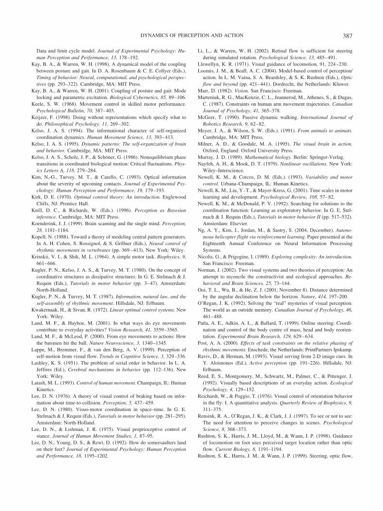
Data and limit cycle model. Journal of Experimental Psychology: Hu-man Perception and Performance, 13, 178–192.

Kay, B. A., & Warren, W. H. (1998). A dynamical model of the couplingbetween posture and gait. In D. A. Rosenbaum & C. E. Collyer (Eds.),Timing of behavior: Neural, computational, and psychological perspec-tives (pp. 293–322). Cambridge, MA: MIT Press.

Kay, B. A., & Warren, W. H. (2001). Coupling of posture and gait: Modelocking and parametric excitation. Biological Cybernetics, 85, 89–106.

Keele, S. W. (1968). Movement control in skilled motor performance.Psychological Bulletin, 70, 387–403.

Keijzer, F. (1998). Doing without representations which specify what todo. Philosophical Psychology, 11, 269–302.

Kelso, J. A. S. (1994). The informational character of self-organizedcoordination dynamics. Human Movement Science, 13, 393–413.

Kelso, J. A. S. (1995). Dynamic patterns: The self-organization of brainand behavior. Cambridge, MA: MIT Press.

Kelso, J. A. S., Scholz, J. P., & Schoner, G. (1986). Nonequilibrium phasetransitions in coordinated biological motion: Critical fluctuations. Phys-ics Letters A, 118, 279–284.

Kim, N,-G., Turvey, M. T., & Carello, C. (1993). Optical informationabout the severity of upcoming contacts. Journal of Experimental Psy-chology: Human Perception and Performance, 19, 179–193.

Kirk, D. E. (1970). Optimal control theory: An introduction. EnglewoodCliffs, NJ: Prentice Hall.

Knill, D. C., & Richards, W. (Eds.). (1996). Perception as Bayesianinference. Cambridge, MA: MIT Press.

Koenderink, J. J. (1999). Brain scanning and the single mind. Perception,28, 1181–1184.

Kopell, N. (1988). Toward a theory of modeling central pattern generators.In A. H. Cohen, S. Rossignol, & S. Grillner (Eds.), Neural control ofrhythmic movements in vertebrates (pp. 369–413). New York: Wiley.

Krinskii, V. I., & Shik, M. L. (1964). A simple motor task. Biophysics, 9,661–666.

Kugler, P. N., Kelso, J. A. S., & Turvey, M. T. (1980). On the concept ofcoordinative structures as dissipative structures. In G. E. Stelmach & J.Requin (Eds.), Tutorials in motor behavior (pp. 3–47). Amsterdam:North-Holland.

Kugler, P. N., & Turvey, M. T. (1987). Information, natural law, and theself-assembly of rhythmic movement. Hillsdale, NJ: Erlbaum.

Kwakernaak, H., & Sivan, R. (1972). Linear optimal control systems. NewYork: Wiley.

Land, M. F., & Hayhoe, M. (2001). In what ways do eye movementscontribute to everyday activities? Vision Research, 41, 3559–3565.

Land, M. F., & McLeod, P. (2000). From eye movements to actions: Howthe batsmen hit the ball. Nature Neuroscience, 3, 1340–1345.

Lappe, M., Bremmer, F., & van den Berg, A. V. (1999). Perception ofself-motion from visual flow. Trends in Cognitive Science, 3, 329–336.

Lashley, K. S. (1951). The problem of serial order in behavior. In L. A.Jeffires (Ed.), Cerebral mechanisms in behavior (pp. 112–136). NewYork: Wiley.

Latash, M. L. (1993). Control of human movement. Champaign, IL: HumanKinetics.

Lee, D. N. (1976). A theory of visual control of braking based on infor-mation about time-to-collision. Perception, 5, 437–459.

Lee, D. N. (1980). Visuo-motor coordination in space–time. In G. E.Stelmach & J. Requin (Eds.), Tutorials in motor behavior (pp. 281–295).Amsterdam: North-Holland.

Lee, D. N., & Lishman, J. R. (1975). Visual proprioceptive control ofstance. Journal of Human Movement Studies, 1, 87–95.

Lee, D. N., Young, D. S., & Rewt, D. (1992). How do somersaulters landon their feet? Journal of Experimental Psychology: Human Perceptionand Performance, 18, 1195–1202.

Li, L., & Warren, W. H. (2002). Retinal flow is sufficient for steeringduring simulated rotation. Psychological Science, 13, 485–491.

Llewellyn, K. R. (1971). Visual guidance of locomotion, 91, 224–230.Loomis, J. M., & Beall, A. C. (2004). Model-based control of perception/

action. In L. M. Vaina, S. A. Beardsley, & S. K. Rushton (Eds.), Opticflow and beyond (pp. 421–441). Dordrecht, the Netherlands: Kluwer.

Marr, D. (1982). Vision. San Francisco: Freeman.Marteniuk, R. G., MacKenzie, C. L., Jeannerod, M., Athenes, S., & Dugas,

C. (1987). Constraints on human arm movement trajectories. CanadianJournal of Psychology, 41, 365–378.

McGeer, T. (1990). Passive dynamic walking. International Journal ofRobotics Research, 9, 62–82.

Meyer, J. A., & Wilson, S. W. (Eds.). (1991). From animals to animats.Cambridge, MA: MIT Press.

Milner, A. D., & Goodale, M. A. (1995). The visual brain in action.Oxford, England: Oxford University Press.

Murray, J. D. (1989). Mathematical biology. Berlin: Springer-Verlag.Nayfeh, A. H., & Mook, D. T. (1979). Nonlinear oscillations. New York:

Wiley–Interscience.Newell, K. M., & Corcos, D. M. (Eds.). (1993). Variability and motor

control. Urbana–Champaign, IL: Human Kinetics.Newell, K. M., Liu, Y.-T., & Mayer-Kress, G. (2001). Time scales in motor

learning and development. Psychological Review, 108, 57–82.Newell, K. M., & McDonald, P. V. (1992). Searching for solutions to the

coordination function: Learning as exploratory behavior. In G. E. Stel-mach & J. Requin (Eds.), Tutorials in motor behavior II (pp. 517–532).Amsterdam: Elsevier.

Ng, A. Y., Kim, J., Jordan, M., & Sastry, S. (2004, December). Autono-mous helicopter flight via reinforcement learning. Paper presented at theEighteenth Annual Conference on Neural Information ProcessingSystems.

Nicolis, G., & Prigogine, I. (1989). Exploring complexity: An introduction.San Francisco: Freeman.

Norman, J. (2002). Two visual systems and two theories of perception: Anattempt to reconcile the constructivist and ecological approaches. Be-havioral and Brain Sciences, 25, 73–144.

Ooi, T. L., Wu, B., & He, Z. J. (2001, November 8). Distance determinedby the angular declination below the horizon. Nature, 414, 197–200.

O’Regan, J. K. (1992). Solving the “real” mysteries of visual perception:The world as an outside memory. Canadian Journal of Psychology, 46,461–488.

Patla, A. E., Adkin, A. L., & Ballard, T. (1999). Online steering: Coordi-nation and control of the body centre of mass, head and body reorien-tation. Experimental Brain Research, 129, 629–634.

Post, A. A. (2000). Effects of task constraints on the relative phasing ofrhythmic movements. Enschede, the Netherlands: PrintPartners Ipskamp.

Raviv, D., & Herman, M. (1993). Visual serving from 2-D image cues. InY. Aloimonos (Ed.), Active perception (pp. 191–226). Hillsdale, NJ:Erlbaum.

Reed, E. S., Montgomery, M., Schwartz, M., Palmer, C., & Pittenger, J.(1992). Visually based descriptions of an everyday action. EcologicalPsychology, 4, 129–152.

Reichardt, W., & Poggio, T. (1976). Visual control of orientation behaviorin the fly: I. A quantitative analysis. Quarterly Review of Biophysics, 9,311–375.

Rensink, R. A., O’Regan, J. K., & Clark, J. J. (1997). To see or not to see:The need for attention to perceive changes in scenes. PsychologicalScience, 8, 368–373.

Rushton, S. K., Harris, J. M., Lloyd, M., & Wann, J. P. (1998). Guidanceof locomotion on foot uses perceived target location rather than opticflow. Current Biology, 8, 1191–1194.

Rushton, S. K., Harris, J. M., & Wann, J. P. (1999). Steering, optic flow,


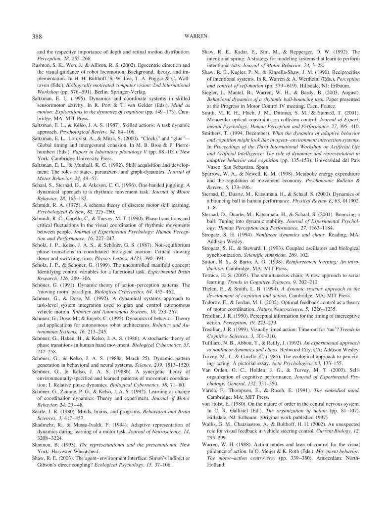
and the respective importance of depth and retinal motion distribution.Perception, 28, 255–266.

Rushton, S. K., Wen, J., & Allison, R. S. (2002). Egocentric direction andthe visual guidance of robot locomotion: Background, theory, and im-plementation. In H. H. Bulthoff, S.-W. Lee, T. A. Poggio & C. Wall-raven (Eds.), Biologically motivated computer vision: 2nd InternationalWorkshop (pp. 576–591). Berlin: Springer-Verlag.

Saltzman, E. L. (1995). Dynamics and coordinate systems in skilledsensorimotor activity. In R. Port & T. van Gelder (Eds.), Mind asmotion: Explorations in the dynamics of cognition (pp. 149–173). Cam-bridge, MA: MIT Press.

Saltzman, E. L., & Kelso, J. A. S. (1987). Skilled actions: A task dynamicapproach. Psychological Review, 94, 84–106.

Saltzman, E. L., Lofqvist, A., & Mitra, S. (2000). “Clocks” and “glue”—Global timing and intergestural cohesion. In M. B. Broe & P. Pierre-humbert (Eds.), Papers in laboratory phonology V (pp. 88–101). NewYork: Cambridge University Press.

Saltzman, E. L., & Munhall, K. G. (1992). Skill acquisition and develop-ment: The roles of state-, parameter-, and graph-dynamics. Journal ofMotor Behavior, 24, 49–57.

Schaal, S., Sternad, D., & Atkeson, C. G. (1996). One-handed juggling: Adynamical approach to a rhythmic movement task. Journal of MotorBehavior, 28, 165–183.

Schmidt, R. A. (1975). A schema theory of discrete motor skill learning.Psychological Review, 82, 225–260.

Schmidt, R. C., Carello, C., & Turvey, M. T. (1990). Phase transitions andcritical fluctuations in the visual coordination of rhythmic movementsbetween people. Journal of Experimental Psychology: Human Percep-tion and Performance, 16, 227–247.

Scholz, J. P., Kelso, J. A. S., & Schoner, G. S. (1987). Non-equilibriumphase transitions in coordinated biological motion: Critical slowingdown and switching time. Physics Letters, A123, 390–394.

Scholz, J. P., & Schoner, G. (1999). The uncontrolled manifold concept:Identifying control variables for a functional task. Experimental BrainResearch, 126, 289–306.

Schoner, G. (1991). Dynamic theory of action–perception patterns: The‘moving room’ paradigm. Biological Cybernetics, 64, 455–462.

Schoner, G., & Dose, M. (1992). A dynamical systems approach totask-level system integration used to plan and control autonomousvehicle motion. Robotics and Autonomous Systems, 10, 253–267.

Schoner, G., Dose, M., & Engels, C. (1995). Dynamics of behavior: Theoryand applications for autonomous robot architectures. Robotics and Au-tonomous Systems, 16, 213–245.

Schoner, G., Haken, H., & Kelso, J. A. S. (1986). A stochastic theory ofphase transitions in human hand movement. Biological Cybernetics, 53,247–258.

Schoner, G., & Kelso, J. A. S. (1988a, March 25). Dynamic patterngeneration in behavioral and neural systems. Science, 239, 1513–1520.

Schoner, G., & Kelso, J. A. S. (1988b). A synergetic theory ofenvironmentally-specified and learned patterns of movement coordina-tion: I. Relative phase dynamics. Biological Cybernetics, 58, 71–80.

Schoner, G., Zanone, P. G., & Kelso, J. A. S. (1992). Learning as changeof coordination dynamics: Theory and experiment. Journal of MotorBehavior, 24, 29–48.

Searle, J. R. (1980). Minds, brains, and programs. Behavioral and BrainSciences, 3, 417–457.

Shadmehr, R., & Mussa-Ivaldi, F. (1994). Adaptive representation ofdynamics during learning of a motor task. Journal of Neuroscience, 14,3208–3224.

Shannon, B. (1993). The representational and the presentational. NewYork: Harvester Wheatsheaf.

Shaw, R. E. (2003). The agent–environment interface: Simon’s indirect orGibson’s direct coupling? Ecological Psychology, 15, 37–106.

Shaw, R. E., Kadar, E., Sim, M., & Repperger, D. W. (1992). Theintentional spring: A strategy for modeling systems that learn to performintentional acts. Journal of Motor Behavior, 24, 3–28.

Shaw, R. E., Kugler, P. N., & Kinsella-Shaw, J. M. (1990). Reciprocitiesof intentional systems. In R. Warren & A. Wertheim (Eds.), Perceptionand control of self-motion (pp. 579–619). Hillsdale, NJ: Erlbaum.

Siegler, I., Mantel, B., Warren, W. H., & Bardy, B. (2003, August).Behavioral dynamics of a rhythmic ball-bouncing task. Paper presentedat the Progress in Motor Control IV meeting, Caen, France.

Smith, M. R. H., Flach, J. M., Dittman, S. M., & Stanard, T. (2001).Monocular optical constraints on collision control. Journal of Experi-mental Psychology: Human Perception and Performance, 27, 395–410.

Smithers, T. (1994, December). What the dynamics of adaptive behaviorand cognition might look like in agent–environment interaction systems.In Proceedings of the Third International Workshop on Artificial Lifeand Artificial Intelligence: The role of dynamics and representation inadaptive behavior and cognition (pp. 135–153). Universidad del PaisVasco, San Sebastian, Spain.

Sparrow, W. A., & Newell, K. M. (1998). Metabolic energy expenditureand the regulation of movement economy. Psychonomic Bulletin &Review, 5, 173–196.

Sternad, D., Duarte, M., Katsumata, H., & Schaal, S. (2000). Dynamics ofa bouncing ball in human performance. Physical Review E, 63, 011902.1–8.

Sternad, D., Duarte, M., Katsumata, H., & Schaal, S. (2001). Bouncing aball: Tuning into dynamic stability. Journal of Experimental Psychol-ogy: Human Perception and Performance, 27, 1163–1184.

Strogatz, S. H. (1994). Nonlinear dynamics and chaos. Reading, MA:Addison Wesley.

Strogatz, S. H., & Steward, I. (1993). Coupled oscillators and biologicalsynchronization. Scientific American, 269, 102.

Sutton, R. S., & Barto, A. G. (1998). Reinforcement learning: An intro-duction. Cambridge, MA: MIT Press.

Terrace, H. S. (2005). The simultaneous chain: A new approach to seriallearning. Trends in Cognitive Sciences, 9, 202–210.

Thelen, E., & Smith, L. B. (1994). A dynamic systems approach to thedevelopment of cognition and action. Cambridge, MA: MIT Press.

Todorov, E., & Jordan, M. I. (2002). Optimal feedback control as a theoryof motor coordination. Nature Neuroscience, 5, 1226–1235.

Tresilian, J. R. (1990). Perceptual information for the timing of interceptiveaction. Perception, 19, 223–239.

Tresilian, J. R. (1999). Visually timed action: Time-out for ‘tau’? Trends inCognitive Sciences, 3, 301–310.

Tufillaro, N. B., Abbott, T., & Reilly, J. (1992). An experimental approachto nonlinear dynamics and chaos. Redwood City, CA: Addison Wesley.

Turvey, M. T., & Carello, C. (1986). The ecological approach to perceiv-ing–acting: A pictorial essay. Acta Psychologica, 63, 133–155.

Van Orden, G. C., Holden, J. G., & Turvey, M. T. (2003). Self-organization of cognitive performance. Journal of Experimental Psy-chology: General, 132, 331–350.

Varela, F., Thompson, E., & Rosch, E. (1991). The embodied mind.Cambridge, MA: MIT Press.

von Holst, E. (1980). On the nature of order in the central nervous system.In C. R. Gallistel (Ed.), The organization of action (pp. 81–107).Hillsdale, NJ: Erlbaum. (Original work published 1937)

Wallis, G. M., Chatziastros, A., & Bulthoff, H. H. (2002). An unexpectedrole for visual feedback in vehicle steering control. Current Biology, 12,295–299.

Warren, W. H. (1988). Action modes and laws of control for the visualguidance of action. In O. Meijer & K. Roth (Eds.), Movement behavior:The motor–action controversy (pp. 339–380). Amsterdam: North-Holland.

388 WARREN

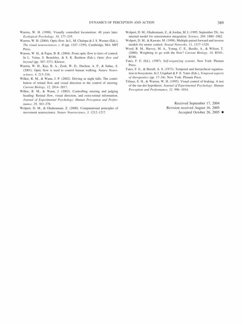
Warren, W. H. (1998). Visually controlled locomotion: 40 years later.Ecological Psychology, 10, 177–219.

Warren, W. H. (2004). Optic flow. In L. M. Chalupa & J. S. Werner (Eds.),The visual neurosciences, v. II (pp. 1247–1259). Cambridge, MA: MITPress.

Warren, W. H., & Fajen, B. R. (2004). From optic flow to laws of control.In L. Vaina, S. Beardsley, & S. K. Rushton (Eds.), Optic flow andbeyond (pp. 307–337): Kluwer.

Warren, W. H., Kay, B. A., Zosh, W. D., Duchon, A. P., & Sahuc, S.(2001). Optic flow is used to control human walking. Nature Neuro-science, 4, 213–216.

Wilkie, R. M., & Wann, J. P. (2002). Driving as night falls: The contri-bution of retinal flow and visual direction to the control of steering.Current Biology, 12, 2014–2017.

Wilkie, R. M., & Wann, J. (2003). Controlling steering and judgingheading: Retinal flow, visual direction, and extra-retinal information.Journal of Experimental Psychology: Human Perception and Perfor-mance, 29, 363–378.

Wolpert, D. M., & Ghahramani, Z. (2000). Computational principles ofmovement neuroscience. Nature Neuroscience, 3, 1212–1217.

Wolpert, D. M., Ghahramani, Z., & Jordan, M. I. (1995, September 29). Aninternal model for sensorimotor integration. Science, 269, 1880–1882.

Wolpert, D. M., & Kawato, M. (1998). Multiple paired forward and inversemodels for motor control. Neural Networks, 11, 1317–1329.

Wood, R. M., Harvey, M. A., Young, C. E., Beedie, A., & Wilson, T.(2000). Weighting to go with the flow? Current Biology, 10, R545–R546.

Yates, F. E. (Ed.). (1987). Self-organizing systems. New York: PlenumPress.

Yates, F. E., & Iberall, A. S. (1973). Temporal and hierarchical organiza-tion in biosystems. In J. Urquhart & F. E. Yates (Eds.), Temporal aspectsof therapeutics (pp. 17–34). New York: Plenum Press.

Yilmaz, E. H., & Warren, W. H. (1995). Visual control of braking: A testof the tau-dot hypothesis. Journal of Experimental Psychology: HumanPerception and Performance, 21, 996–1014.

Received September 17, 2004Revision received August 16, 2005

Accepted October 26, 2005 �


Documents

The Dynamics of Perception and Action - IGERT