HAL Id: hal-01025351https://hal-polytechnique.archives-ouvertes.fr/hal-01025351

Submitted on 11 Sep 2014

HAL is a multi-disciplinary open accessarchive for the deposit and dissemination of sci-entific research documents, whether they are pub-lished or not. The documents may come fromteaching and research institutions in France orabroad, or from public or private research centers.

L’archive ouverte pluridisciplinaire HAL, estdestinée au dépôt et à la diffusion de documentsscientifiques de niveau recherche, publiés ou non,émanant des établissements d’enseignement et derecherche français ou étrangers, des laboratoirespublics ou privés.

The dynamics of a viscous soap film with solublesurfactant

Jean-Marc Chomaz

To cite this version:Jean-Marc Chomaz. The dynamics of a viscous soap film with soluble surfactant. Jour-nal of Fluid Mechanics, Cambridge University Press (CUP), 2001, 442 (september), pp.387-409.�10.1017/s0022112001005213�. �hal-01025351�

J. Fluid Mech. (2001), vol. 442, pp. 387–409. Printed in the United Kingdom

c© 2001 Cambridge University Press

387

The dynamics of a viscous soap film withsoluble surfactant

By JEAN-MARC CHOMAZ

LadHyX, CNRS–Ecole Polytechnique, 91128 Palaiseau, France

(Received 25 October 1999 and in revised form 24 March 2001)

Nearly two decades ago, Couder (1981) and Gharib & Derango (1989) used soap filmsto perform classical hydrodynamics experiments on two-dimensional flows. Recentlysoap films have received renewed interest and experimental investigations publishedin the past few years call for a proper analysis of soap film dynamics. In the presentpaper, we derive the leading-order approximation for the dynamics of a flat soap filmunder the sole assumption that the typical length scale of the flow parallel to the filmsurface is large compared to the film thickness. The evolution equations governingthe leading-order film thickness, two-dimensional velocities (locally averaged acrossthe film thickness), average surfactant concentration in the interstitial liquid, andsurface surfactant concentration are given and compared to similar results from theliterature. Then we show that a sufficient condition for the film velocity distributionto comply with the Navier–Stokes equations is that the typical flow velocity besmall compared to the Marangoni elastic wave velocity. In that case the thicknessvariations are slaved to the velocity field in a very specific way that seems consistentwith recent experimental observations. When fluid velocities are of the order of theelastic wave speed, we show that the dynamics are generally very specific to a soapfilm except if the fluid viscosity and the surfactant solubility are neglected. In thatcase, the compressible Euler equations are recovered and the soap film behaves like atwo-dimensional gas with an unusual ratio of specific heat capacities equal to unity.

1. Introduction

Water films have been studied since the pioneering papers of Savart (1833a, b), Boys(1890), and, later, of Squire (1953) and Taylor (1959) because of their natural beauty,their theoretical interest, and the variety of applications ranging from atomizationand sprays in combustion to curtain coating processes. Water films sustain wavesoriginating from the interactions between the capillary waves which develop on theirinterfaces.

When soap is added to water, the dependence of surface tension on the superficialsoap concentration makes the film elastic and therefore reduces its tendency tobreak. In this case, the soap film may sustain large-scale in-plane motions. Thisproperty has allowed soap films to be used as a convenient two-dimensional fluid.In Couder’s (1981) experiments a membrane, stretched on a large frame, was usedas a two-dimensional towing tank. Further investigations were reported by Gharib& Derango (1989) who designed a soap tunnel by pulling a horizontal membranedownstream of the test section with a clear water jet. Recently, a new way to producea soap tunnel has been proposed and tested by Kellay, Wu & Goldburg (1995). Intheir experiment a vertical membrane is continuously stretched between two wires

388 J.-M. Chomaz

emerging from a reservoir from which soap solution is twinkling down. These soap filmexperiments have attracted the curiosity of numerous scientists who have performedmodern, careful, and precise mesurements of various two-dimensional flows such as,in particular, Wu et al. (1995), Kellay et al. (1995, 1998), Rutgers, Wu & Bhagavatula(1996), Goldburg, Rutgers & Wu (1997), Afenchenko et al. (1998), Martin et al.(1998), Rivera, Vorobieff & Ecke (1998), Vega, Higuera & Wiedman (1998), Vorobieff,Rivera & Ecke (1999), Boudaoud, Couder & Ben Amar (1999), Burgess et al. (1999),Horvath et al. (2000), Rivera & Wu (2000).

Despite this continuous interest, a fundamental question remains unanswered:whether soap films obey the classical two-dimensional Navier–Stokes equations and,for example, demonstrate the existence of the inverse cascade in two-dimensionalturbulence, or soap films suffer specific dynamics that make them useless for theinvestigation of fundamental problems of two-dimensional hydrodynamics? On thesolution of this dilemma depends the pertinence of soap film experiments. On thebasis of appropriate physical considerations, Couder, Chomaz & Rabaud (1989) (andlater on Chomaz & Cathalau 1990, and Chomaz & Costa 1998) have shown thata two-dimensional description may be achieved if the velocity is small compared tothe elastic wave velocity. But as yet, no proper demonstrations have validated theirassumptions; furthermore no results at all are at present available for when the soapfilm velocity is close to the elastic wave velocity.

In § 3 of the present contribution a complete analysis of the three-dimensional soapfilm dynamics is presented using the asymptotic lubrication theory which assumesonly that the thickness of the film is small compared to the characteristic length scaleof the in-plane flow. The analysis gives both the physics of the equilibrium at playin the free film and the order of magnitude of the neglected effects. The paper willmake systematic use of the notations and results of recent contributions by Edwards& Oron (1995) and Oron, Davis & Bankoff (1997) to which the reader shouldrefer. The mathematical analysis of thin film dynamics using asymptotic expansions,multiple scale analysis, the long wave assumption or equivalently the homogenizationtechnique is standard and applications to free films and films coating a solid surfacehave been reviewed in Oron et al. (1997) and Ida & Miksis (1998a). Only a fewparticular contributions are mentioned here. Evolution equations for the surfactanthave been derived in Waxman (1984) and Stone (1990). The nonlinear dynamics oftwo-dimensional free films may be found in Prevost & Gallez (1986) and in Erneux& Davis (1993) for the case without surfactant, and in Sharma & Ruckenstein (1986)and De Wit, Gallez & Christov (1994) for the case with insoluble surfactant. Thethree-dimensional dynamics of an arbitrary film have been analysed by van de Fliert,Howell & Ockendon (1995) and extended by Ida & Miksis (1998a) to take surfactanteffects into account. Section 3 of the present contribution may be viewed as anapplication to a planar geometry of the general description given by Ida & Miksis(1998b). It extends the latter study by including surfactant solubility and derivingthe associated evolution equation for the averaged surfactant concentration in theinterstitial liquid.

Although the present derivation of § 3 shares results with De Wit et al. (1994) andIda & Miksis (1998a, b) it differs from them by the scaling assumption: previousstudies concentrate on the motion induced by surfaces or van der Waals forceswhereas, here, we consider the fate of pre-existing motion. As a result, the order ofmagnitude of the planar velocity is treated as a free parameter instead of being fixedby viscous effects. This leads to new scalings for the velocity, the pressure, the thicknessvariation, and the time scales and imposes the introduction of new non-dimensional

Soap film dynamics 389

2Hy

x

z

n

c

è

C

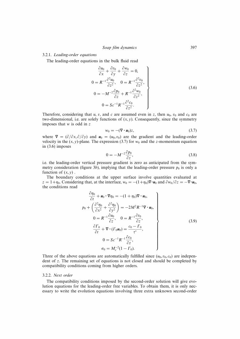
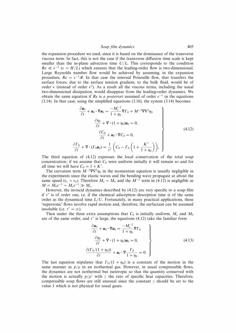
Figure 1. Soap film internal structure.

parameters. The leading-order equations so obtained are specific to soap films andtheir relations to the Navier–Stokes equations are discussed in § 4. We make use ofthe flexibility brought by the new scaling assumptions and consider different limitcases, only one of which results in incompressible two-dimensional Navier–Stokesdynamics and another in the compressible Euler equations for a two-dimensional gaswith an unusual ratio of specific heats γ = 1. In no cases will a soap film satisfythe compressible two-dimensional Navier–Stokes equations. The importance of theratio between the typical planar velocity and the elastic Marangoni wave velocity isrigorously established.

2. Soap film equations

As described in Couder et al. (1989), soap films used in hydrodynamics experimentsmay be seen as a three-layer structure: two surfaces and a bulk fluid in-between (fig-ure 1). For simplicity, a single species of surfactant will be considered, this surfactant(from now on called the soap) being allowed to migrate between the three phases(soluble surfactant). The film is considered flat as is indeed the case in vertical soapfilm experiments or when the bending of the soap film under its weight is compen-sated by a pressure difference between the two surfaces (see Couder et al. 1989 fordetails). Only symmetric perturbations will be considered and, therefore, each surfacephase will be a mirror of the other. The surface concentration of soap will be denotedby Γ whereas c will designate the interstitial soap concentration.

The bulk fluid moves with a three-dimensional velocity u = (u, v, w). The fluidis assumed incompressible with a density ρ and a kinematic viscosity ν = µ/ρindependent of the amount of soap. The pressure inside the film is denoted p.The two surface phases are symmetrically deformed and located at the elevationz = ±η(x, y, t), the film being assumed flat on average in the plane (x, y). A surfacetension σ applies to each surface.

The bulk fluid flow is governed by the incompressible Navier–Stokes equation andthe bulk soap concentration by the advection diffusion equation:

∇∗

· u = 0,

∂u

∂t+ u · ∇

∗u = −

1

ρ∇

∗p + ν∇∗2u,

∂c

∂t+ u · ∇

∗c = D∇∗2c,

(2.1)

390 J.-M. Chomaz

where D is the soap diffusivity in the bulk fluid and ∇∗ stands for the three-dimensional

nabla operator in order to differentiate it from its two-dimensional counterpart (inthe x, y-plane) denoted ∇.

Although potential volume forces, like gravity or van der Waals forces, may betaken into account by adding a ∇

∗φ term on the right-hand side of the momentumequation (2.1) (see Edwards & Oron 1995; Ida & Miksis 1995, 1998a; and Oron et al.1997 for details), they will be ignored as a first step. This assumption is realistic, sincesoap films used in experiments are a few microns thick, so that direct interactionsbetween surfaces (van der Waals forces possibly represented by a disjoining pressure)are negligible.

This system of bulk fluid equations is completed by boundary conditions at bothfree surfaces and because of the assumed symmetry only the conditions at the uppersurface will be explicitly given. The kinematic condition, at the interface z = η(x, y, t),reads

∂η

∂t+ u · ∇

∗η = w, (2.2)

whereas the force balance at each interface may be written

(p − pa + 2Cσ)n = ∇sσ + µ(∇∗u + ∇

∗ut) · n, (2.3)

following Levich & Krylov (1969) and using the notation of Edwards & Oron (1995).The pressure in the air surrounding the film is denoted by pa, the unit vector normalto the upper surface and oriented toward the air by n with

n =

(

−∂η

∂x,−

∂η

∂y, 1

)

(

1 +

(

∂η

∂x

)2

+

(

∂η

∂y

)2)−1/2

, (2.4)

2C is the mean surface curvature (defined by 2C = −∇∗

· n)

2C =

∂2η

∂x2

(

1 +

(

∂η

∂y

)2)

− 2∂η

∂x

∂η

∂y

∂2η

∂x∂y+

∂2η

∂y2

(

1 +

(

∂η

∂x

)2)

(

1 +

(

∂η

∂x

)2

+

(

∂η

∂y

)2)3/2

, (2.5)

∇s the surface gradient operator

∇s = Is · ∇∗, (2.6)

with Is the surface idemfactor

Is = I − nn (I the spatial idemfactor). (2.7)

The left-hand side of equation (2.3) corresponds simply to the Young–Laplace lawwhich states that surface tension induces a jump in pressure when the interface iscurved. Equation (2.3) projected on the normal n gives

p − pa + 2Cσ = n · µ(∇∗u + ∇

∗ut) · n. (2.8)

The right-hand side of equation (2.3) expresses the balance at the interface betweenthe surface tension gradient and the tangential shear stress in the bulk fluid µ(∇∗

u +∇

∗ut) · n. Projected on the two tangents to the interface (not normalized) t1 =

(1, 0, ∂η/∂x) and t2 = (0, 1, ∂η/∂y) equation (2.3) gives

0 = ∇sσ · ti + ti · µ(∇∗u + ∇

∗ut) · n. (2.9)

Soap film dynamics 391

Terms, like for example µs∇2s u, may also be added to equation (2.3) to express

dissipation in the surface layer due to surface shear viscosity µs generated by theadsorbed surfactant. In the present study, such terms will not be considered, althoughtheir introduction is straightforward, because the dissipation in the bulk fluid isassumed to dominate for such a thick film.

Except when soap films are flowing into vacuum, air friction should also enterequation (2.3) through an extra term −µa(∇

∗ua + ∇

∗ua

t) · n on the right-hand side,where ua and −µa are the air velocity and viscosity. This effect has been discussedin Couder et al. (1989), and although it has been shown to be important (see inparticular Rivera & Wu 2000), it is not included here to ease the derivation. Furthercomments are made later on. Furthermore evaporation of water, essential for thinnerfilms, might be also considered as discussed in Oron et al. (1997).

The present paper will concentrate on the leading-order equation governing theevolution of large-scale motions imposed by moving boundaries normal to the filmsurface (as moving disks or cylinders). The precise details of the interaction withthe boundary that involves a meniscus (see Couder et al. 1989) will not be de-scribed. We will simply consider the initial-value problem without lateral (normalto the film surface) boundaries where a large-scale flow (generally non-potential) isinitially imposed arbitrarily. Experimentally the generation of vorticity by laterallymoving walls could be avoided by using an electromagnetic field to generate a bodyforce in the plane of the film. This technique was very efficient in generating two-dimensional turbulence in thin stratified extended layers by Paret & Tabeling (1997).It has been very recently implemented with soap films by Riviera & Wu (2000) whohave experimentally demonstrated the validity of the two-dimensional Navier–Stokesapproximation for soap film dynamics. Another technique to generate initial motionin the film without a wall in conttact with the soap film uses air friction and has beensuccessfully applied by Burgess et al. (1999) to study the stability of Kolmogorovflow.

To solve the last equation of the system (2.1), we need a condition on the bulksoap concentration c at the boundary. Following Levich & Krylov (1969), let us callthe flux of soap from the bulk film to the surface j, then

Dn · ∇∗c = −j,

∂Γ

∂t+ ∇s · (uΓ ) = Ds∇

2sΓ + j,

}

(2.10)

where Ds is the surface diffusivity of a soap molecule that will be neglected (as wedid for the surface viscosity) since the typical length scale of the in-plane motionis considered to be large compared to the thickness of the film. We shall assumethat the flux j is dictated by an adsorption–desorption process given by a first-orderkinetics:

j = (Kc − Γ )/τ, (2.11)

where τ is the adsorption–desorption time and Kc is the instantaneous equilibriumsurface density, K being a coefficient with the dimension of a length that maybe interpreted as the virtual thickness of the interface in terms of soap moleculeadsorption. Since soap molecules, composed of a hydrophilic polar head associatedwith an hydrophobic carbon tail, tend to settle at the surface, K is large (of theorder of 4 µm for sodium dodecyl sulfate (SDS) following Rusanov & Krotov 1979)and τ may be large too (from an order of 10−2 s for a pure single surfactant agentto an order of 1 s or more when impurities or different surfactants are present;

392 J.-M. Chomaz

(a)

(b)

(c)

c i

c i

c f

r f

r f

r f

r f

ri

riC i

C f

C f

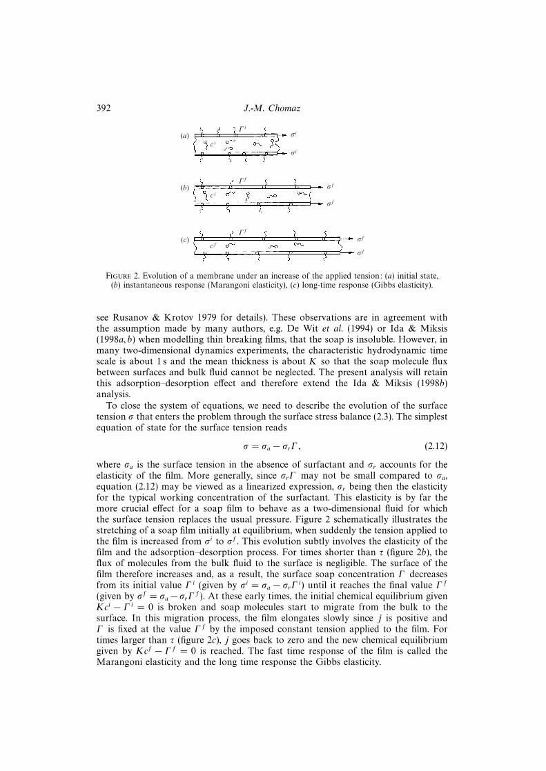
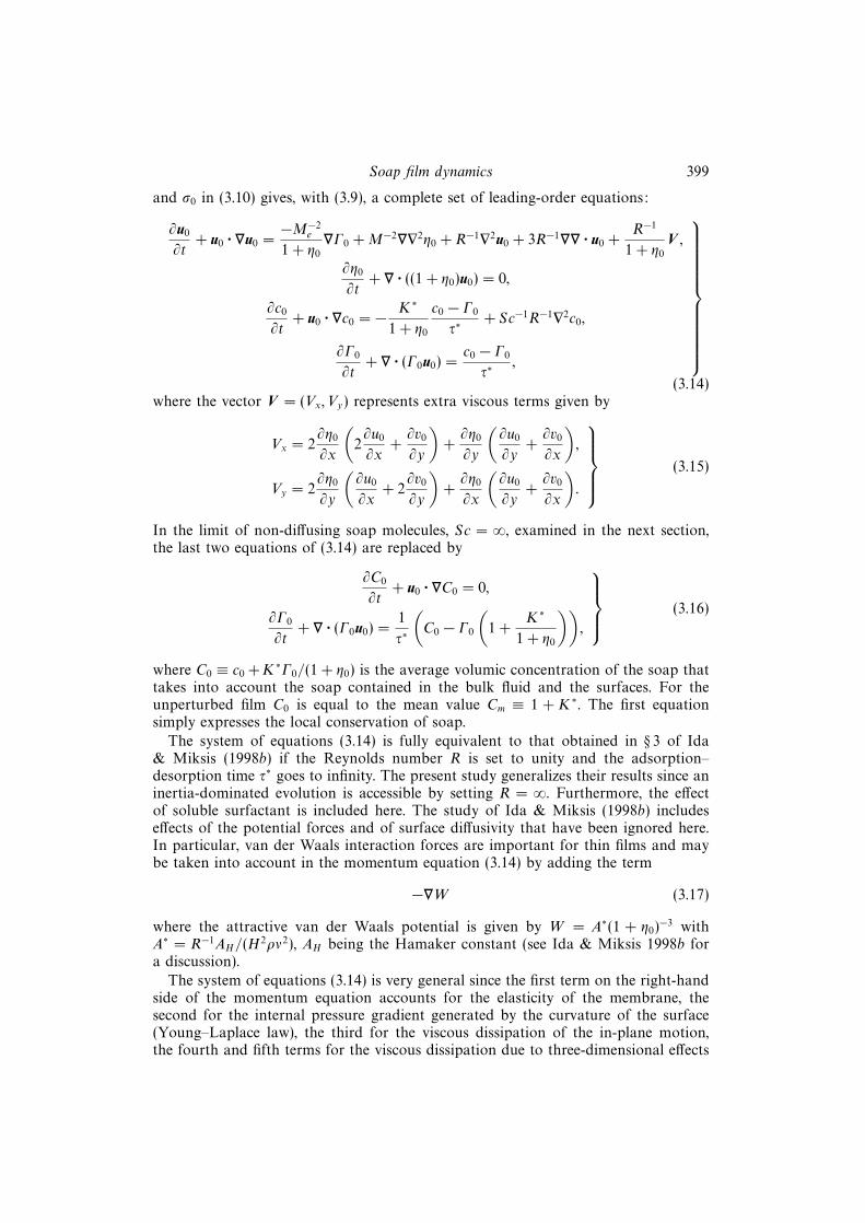
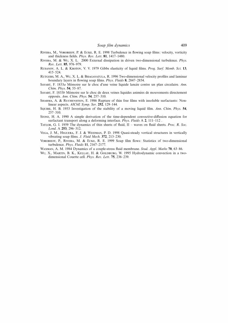
Figure 2. Evolution of a membrane under an increase of the applied tension: (a) initial state,(b) instantaneous response (Marangoni elasticity), (c) long-time response (Gibbs elasticity).

see Rusanov & Krotov 1979 for details). These observations are in agreement withthe assumption made by many authors, e.g. De Wit et al. (1994) or Ida & Miksis(1998a, b) when modelling thin breaking films, that the soap is insoluble. However, inmany two-dimensional dynamics experiments, the characteristic hydrodynamic timescale is about 1 s and the mean thickness is about K so that the soap molecule fluxbetween surfaces and bulk fluid cannot be neglected. The present analysis will retainthis adsorption–desorption effect and therefore extend the Ida & Miksis (1998b)analysis.

To close the system of equations, we need to describe the evolution of the surfacetension σ that enters the problem through the surface stress balance (2.3). The simplestequation of state for the surface tension reads

σ = σa − σrΓ , (2.12)

where σa is the surface tension in the absence of surfactant and σr accounts for theelasticity of the film. More generally, since σrΓ may not be small compared to σa,equation (2.12) may be viewed as a linearized expression, σr being then the elasticityfor the typical working concentration of the surfactant. This elasticity is by far themore crucial effect for a soap film to behave as a two-dimensional fluid for whichthe surface tension replaces the usual pressure. Figure 2 schematically illustrates thestretching of a soap film initially at equilibrium, when suddenly the tension applied tothe film is increased from σi to σf . This evolution subtly involves the elasticity of thefilm and the adsorption–desorption process. For times shorter than τ (figure 2b), theflux of molecules from the bulk fluid to the surface is negligible. The surface of thefilm therefore increases and, as a result, the surface soap concentration Γ decreasesfrom its initial value Γ i (given by σi = σa − σrΓ

i) until it reaches the final value Γ f

(given by σf = σa − σrΓf). At these early times, the initial chemical equilibrium given

Kci − Γ i = 0 is broken and soap molecules start to migrate from the bulk to thesurface. In this migration process, the film elongates slowly since j is positive andΓ is fixed at the value Γ f by the imposed constant tension applied to the film. Fortimes larger than τ (figure 2c), j goes back to zero and the new chemical equilibriumgiven by Kcf − Γ f = 0 is reached. The fast time response of the film is called theMarangoni elasticity and the long time response the Gibbs elasticity.

Soap film dynamics 393

(a) (b)

r

r

r

r

pa

pa

r

r

r

r

pa

pa

¢

p

¢

p

¢

p

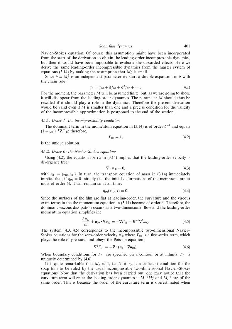
Figure 3. Pressure gradient in the case of (a) antisymmetric mode (bending mode)and (b) symmetric mode.

3. Non-dimensional problem and asymptotic expansion

Before presenting the asymptotic expansion of the problem, it is worth pointingout that the soap film hydrodynamics considered here involve in-plane motion with alarge length scale L compared to the mean film thickness 2H . Therefore, we anticipatethat the pressure will be everywhere constrained by the Young–Laplace law, varyingas σa2C, the mean curvature C being at most of order H/L2. At leading order, thepressure gradient will play no role and only viscous forces will be able to balancethe surface tension gradient (describing the elasticity of the membrane) in the surfacestress equation (2.3). In turn, viscous terms due to velocity shear in the z-direction willdominate in the Navier–Stokes equation (2.1) and transfer the surface force (due tothe elasticity) to the bulk fluid. As already pointed out by Taylor (1959) the balancesat work in free films radically differ from those in thin films on a solid surface. Inthe latter case, the pressure is given by the hydrostatic balance at leading order andis compensated by viscous stresses with inertia terms being important at the nextorder. Therefore, the non-dimensionalization will differ from that of Edwards & Oron(1995).

In Ida & Miksis (1998a) the film is not flat. Curvature is then of order L−1, thepressure gradient is dominant and it is balanced by the inertia normal to the centre-surface (see figure 3 and the discussion of § 3.2). This effect deforms the centre-surfaceas if it were an elastic membrane. At next order the balance described above isrecovered.

3.1. Non-dimensional problem

The indirect balance between surface forces and bulk film inertia, anticipated above,has already been described in Couder et al. (1989) and analysed in De Wit et al. (1994)and Ida & Miksis (1998a, b) (referred to herein as DWGC & IM) for the breakingof a film initially at rest. We shall extend their analysis to the situation where thevelocity in the plane of the film is arbitrarily prescribed initially. The typical velocityin the present analysis is a free parameter (whereas in DWGC & IM it is imposedby the surface interaction and viscosity). Therefore, the non-dimensionalization willdiffer from DWGC & IM to allow more flexibility. Furthermore, we shall considersoluble surfactants and this will add a new degree of freedom in the asymptoticleading-order equations. The basic structure of the flow will turn out to be the onedescribed physically by Couder et al. (1989), i.e. a leading-order flow, uniform overthe depth of the film, coupled to a Poiseuille secondary flow that uniformly transfersthe surface elasticity forces to the bulk fluid. The following asymptotic expansioninspired by DWGC & IM will rigorously establish this particular interplay betweensurface and bulk forces and between primary and secondary flows. The full derivation

394 J.-M. Chomaz

is still given since it throws light on the origin of each term of the leading-orderequation and is therefore necessary to understand the physical mechanism at playin the various dominant balances considered in § 4. For the first time, the governingequations for mean velocities, the bulk and surface surfactant concentrations, andfilm thickness are given for three-dimensional motion of a free film with solublesurfactant.

Let ǫ = H/L be the expansion parameter and anticipating the dominant balanceprinciple we non-dimensionalize the variables as

x = x′L, y = y′L, z = z′H = ǫz′L,

u = u′U, v = v′U, w = ǫw′U,

t = t′L/U, p = pa + p′ǫσm/L, σ = σm + σ′ρHU2 = σm + ǫσ′ρLU2,

η = (1 + η′)H, Γ = Γ ′Γm, c = c′cm,

(3.1)

where U is the characteristic velocity, Γm and cm are, respectively, the surfaceand bulk mean concentrations of soap defined by Γm = Kcm such that Cm ≡Γm/H + cm = cm(1 + K/H) is the typical total soap concentration of the solutionfrom which the membrane has been made. The mean surface tension of the film isσm = σa − σrΓm. The pressure variations have been scaled by ǫσm/L anticipating adominant balance due to the Young–Laplace law. Then, the non-dimensional bulkequations reduce to, dropping the primes of all non-dimensionalized quantities forconvenience,

∂u

∂x+

∂v

∂y+

∂w

∂z= 0,

∂u

∂t+ u

∂u

∂x+ v

∂u

∂y+ w

∂u

∂z= −M−2 ∂p

∂x+ R−1

(

∂2u

∂x2+

∂2u

∂y2+ ǫ−2 ∂

2u

∂z2

)

,

∂v

∂t+ u

∂v

∂x+ v

∂v

∂y+ w

∂v

∂z= −M−2 ∂p

∂y+ R−1

(

∂2v

∂x2+

∂2v

∂y2+ ǫ−2 ∂

2v

∂z2

)

,

∂w

∂t+ u

∂w

∂x+ v

∂w

∂y+ w

∂w

∂z= −ǫ−2M−2 ∂p

∂z+ R−1

(

∂2w

∂x2+

∂2w

∂y2+ ǫ−2 ∂

2w

∂z2

)

,

∂c

∂t+ u

∂c

∂x+ v

∂c

∂y+ w

∂c

∂z= Sc−1R−1

(

∂2c

∂x2+

∂2c

∂y2+ ǫ−2 ∂

2c

∂z2

)

,

(3.2)

where M = Mbǫ−1, with Mb = U/vb the bending Mach number since it compares the

bending mode speed vb =√

σm/Hρ (the bending mode is the antisymmetric modeof the membrane motion due to the tension of the film and for which the elasticityplays no role, see figure 3a) to the flow velocity U, and R = UL/ν is the Reynoldsnumber. The Schmidt number of the soap is Sc = ν/D.

This set of equations is closed by boundary conditions at z = 1 + η (the con-ditions at z = −1 − η are symmetric). The non-dimensional equations (2.2), (2.8),(2.9), (2.10), (2.11), (2.12) read at the lowest order in ǫ required to carried on thepresent asymptotic analysis (see Edwards & Oron 1995 for a systematic expansion of

Soap film dynamics 395

all the relevant quantities)

∂η

∂t+ u

∂η

∂x+ v

∂η

∂y= w,

p + 2C(1 + ǫ2M2σ) = 2M2R−1

(

∂w

∂z−

∂η

∂x

∂u

∂z−

∂η

∂y

∂v

∂z+ O(ǫ2)

)

,

2C =∂2η

∂x2+

∂2η

∂y2+ O(ǫ2),

∂σ

∂x= ǫ−2R−1

(

∂u

∂z+ ǫ2

(

−2∂η

∂x

∂u

∂x−

∂η

∂y

(

∂u

∂y+

∂v

∂x

)

+∂w

∂x

−∂η

∂x

2 ∂u

∂z−

∂η

∂x

∂η

∂y

∂v

∂z+ 2

∂η

∂x

∂w

∂z

)

+ O(ǫ4)

)

,

∂σ

∂y= ǫ−2R−1

(

∂v

∂z+ ǫ2

(

−2∂η

∂y

∂v

∂y−

∂η

∂x

(

∂v

∂x+

∂u

∂y

)

+∂w

∂y

−∂η

∂y

2 ∂v

∂z−

∂η

∂x

∂η

∂y

∂v

∂z+ 2

∂η

∂y

∂w

∂z

)

+ O(ǫ4)

)

,

∂Γ

∂t+

∂(uΓ )

∂x+

∂(vΓ )

∂y=

c − Γ

τ∗+ O(ǫ2),

−K∗(c − Γ )

τ∗= ǫ−2Sc−1R−1

(

∂c

∂z+ O(ǫ2)

)

,

σ = M−2e (1 − Γ ),

(3.3)

where all the quantities are evaluated at z = 1+η, η being a priori of order unity. Thenon-dimensional adsorption–desorption time is represented by τ∗ = τU/L and thevirtual thickness of the interface by K∗ = K/H . The elastic Mach number Me = U/veis the ratio of the flow velocity U to the elastic wave velocity ve defined by (seeLucassen et al. 1970)

ve =

√

σrΓm

ρH. (3.4)

3.2. Asymptotic expansion

We shall now proceed to an asymptotic expansion in ǫ. To do so we have to imposesome constraints on the magnitude of the parameters (R, Sc, M, Me, τ

∗, K∗) in order toensure the well posedness of the expansion while keeping as many physical phenomenaas possible (see Bender & Orszag 1978). Of course, if one is interested in a particularlimit, such as the two-dimensional incompressible or inviscid case, a much simpleranalysis of equations (3.2), (3.3) may be carried out directly using more restrictiveassumptions on the magnitude of the parameters. However, a general approach willbe adopted here and particular limits will be derived from the master leading-orderequations by letting parameters become large or small. One might wonder about thevalidity of such a posteriori changes in the magnitude of the parameters. In fact, thedynamics given by the master equations are identical to those that would have been

396 J.-M. Chomaz

obtained directly provided the dominant term, at present the vertical viscous term,in the bulk equation is not modified. When a different magnitude of the Reynoldsnumber will be considered a special comment on the validity of the expansion willbe made. In all other cases the direct derivation is left to the curious readers.

Although the gauge functions (R, Sc, M) could be fixed using the dominant balanceprinciple, we shall infer them from simple physical considerations. The crucial con-dition is that the transverse diffusion time scale H2/ν should be small comparedto the spanwise advection time scale L/U for the motion to be two-dimensional atleading order. This implies that Rǫ2 ≪ 1 and corresponds to the usual lubricationapproximation. We shall choose the gauge function R = O(1) in order to keep thein-plane viscous effect of the same order as the inertia. The choice R = O(ǫ−1) will bementioned in the last section and corresponds to the in-plane inviscid limit. Similarly,the condition that the soap concentration be at leading-order homogeneous acrossthe film, imposes ScRǫ2 ≪ 1. We shall simply choose Sc of order unity even thoughactually Sc may be relatively large.

One must be careful about the pressure term in the z-momentum equation (3.2)since this term is large, ǫ−2M−2 = Mb

−2 = v2b/U

2, and would be unbalanced withoutany further assumptions. Indeed, the bending wave velocity, which typically variesbetween 2 and 8 m s−1 in the experiments, is much larger than the mean velocity of theflow (10−2 to 1 m s−1). The symmetry of the perturbation must be invoked to clarifythis apparent paradox. If the perturbations of the two surfaces were antisymmetric(figure 3a), the pressure gradient normal to the film would be indeed the dominantterm. This effect corresponds to the transfer (thanks to the pressure gradient in the z-direction) of the force resulting from the curvature of both surfaces of the membraneto the bulk fluid. The whole film, when antisymmetrically deformed (figure 3a), is thenbrought back to the horizontal position as if it were a solid membrane under a tensionequal to twice the surface tension of the soap film. However, since only symmetricperturbations of the interfaces are considered in the present case, the pressure mustbe even in z implying that the leading-order transverse pressure gradient is zero(figure 3b). Only the in-plane pressure gradient may contribute in the leading-orderdynamics. The scaling M = O(1), equivalent to Mb = Mǫ, realizes the balance withthe inertia. Note that in Ida & Miksis (1998a) Mb is kept order unity. Under suchcircumstances, the leading-order dynamics correspond to the bending motion and thedynamics described here arise at the next order.

Finally, the non-dimensional adsorption–desorption time τ∗ and the virtual thick-ness of the interface K∗ will be assumed of order unity. This means that the chemicalrelaxation is allowed to act on the dynamical time scale L/U and that bulk fluid is asoap reservoir with, per unit surface of film, a number soap molecules diluted in thebulk fluid of the same magnitude as the number of soap molecules adsorbed on thesurfaces. Fast adsorption–desorption processes will simply correspond to τ∗ = 0 andthe surface soap concentration Γ will follow instantaneously the bulk concentrationc evaluated at the interface. Equilibrium between the surface soap concentration andthe bulk mean concentration will then be only limited by the diffusion of soap in theinterstitial liquid as described by the last equation in the system (3.2).

Last but not least, the order of magnitude of the elastic Mach number Me doesnot need to be specified since it appears in a single equation and may be consideredas an independent expansion parameter.

Then, all the variables are expanded in series of ǫ2 with the notation

f = f0 + ǫ2f2 + · · · . (3.5)

Soap film dynamics 397

3.2.1. Leading-order equations

The leading-order equations in the bulk fluid read

∂u0

∂x+

∂v0

∂y+

∂w0

∂z= 0,

0 = R−1 ∂2u0

∂z2, 0 = R−1 ∂

2v0

∂z2,

0 = −M−2 ∂p0

∂z+ R−1 ∂

2w0

∂z2,

0 = Sc−1R−1 ∂2c0

∂z2.

(3.6)

Therefore, considering that u, v, and c are assumed even in z, then u0, v0 and c0 aretwo-dimensional, i.e. are solely functions of (x, y). Consequently, since the symmetryimposes that w is odd in z

w0 = −(∇ · u0)z, (3.7)

where ∇ = (∂/∂x, ∂/∂y) and u0 = (u0, v0) are the gradient and the leading-ordervelocity in the (x, y)-plane. The expression (3.7) for w0 and the z-momentum equationin (3.6) imposes

0 = −M−2 ∂p0

∂z, (3.8)

i.e. the leading-order vertical pressure gradient is zero as anticipated from the sym-metry consideration (figure 3b), implying that the leading-order pressure p0 is only afunction of (x, y) .

The boundary conditions at the upper surface involve quantities evaluated atz = 1+η0. Considering that, at the interface, w0 = −(1+η0)∇·u0 and ∂w0/∂z = −∇·u0,the conditions read

∂η0

∂t+ u0 · ∇η0 = −(1 + η0)∇ · u0,

p0 +

(

∂2η0

∂x2+

∂2η0

∂y2

)

= −2M2R−1∇ · u0,

0 = R−1 ∂u0

∂z, 0 = R−1 ∂v0

∂z,

∂Γ0

∂t+ ∇ · (Γ0u0) =

c0 − Γ0

τ∗,

0 = Sc−1R−1 ∂c0

∂z,

σ0 = M−2e (1 − Γ0).

(3.9)

Three of the above equations are automatically fulfilled since (u0, v0, c0) are indepen-dent of z. The remaining set of equations is not closed and should be completed bycompatibility conditions coming from higher orders.

3.2.2. Next order

The compatibility conditions imposed by the second-order solution will give evo-lution equations for the leading-order free variables. To obtain them, it is only nec-essary to write the evolution equations involving three extra unknown second-order

398 J.-M. Chomaz

fields (u2, v2, c2):

∂u0

∂t+ u0 · ∇u0 = −M−2 ∂p0

∂x+ R−1

(

∂2u0

∂x2+

∂2u0

∂y2+

∂2u2

∂z2

)

,

∂v0

∂t+ u0 · ∇v0 = −M−2 ∂p0

∂y+ R−1

(

∂2v0

∂x2+

∂2v0

∂y2+

∂2v2

∂z2

)

,

∂c0

∂t+ u0 · ∇c0 = Sc−1R−1

(

∂2c0

∂x2+

∂2c0

∂y2+

∂2c2

∂z2

)

,

(3.10)

and three boundary conditions at z = 1+η0 (these equations do not involve η2 terms):

∂σ0

∂x= R−1

(

∂u2

∂z− Ax

)

,

∂σ0

∂y= R−1

(

∂v2

∂z− Ay

)

,

−K∗ c0 − Γ0

τ∗= Sc−1R−1 ∂c2

∂z,

(3.11)

where Ax and Ay are shear stresses at the interface coming from the zeroth-ordersolution:

Ax = 2∂η0

∂x

∂u0

∂x+

∂η0

∂y

(

∂u0

∂y+

∂v0

∂x

)

+ (1 + η0)∂∇ · u0

∂x+ 2

∂η0

∂x∇ · u0,

Ay = 2∂η0

∂y

∂v0

∂y+

∂η0

∂x

(

∂u0

∂y+

∂v0

∂x

)

+ (1 + η0)∂∇ · u0

∂y+ 2

∂η0

∂y∇ · u0.

(3.12)

Recalling that the symmetry imposes that (u, v, c) are even in z, equations (3.10) showthat (u2, v2, c2) are parabolic in z (Poiseuille like) since all the other terms involvethe zeroth-order solution which does not vary with z. The boundary conditions (3.11)state that shear stresses associated with the vertical variations of (u2, v2) compensatezeroth-order shear stresses and surface tension gradient. Similarly, the second-ordersoap diffusive flux in the bulk fluid equilibrates the soap flux from the surface dueto zeroth-order quantities. These boundary conditions (3.11) gives the expressions for(u2, v2, c2):

u2 =

(

R∂σ0

∂x+ Ax

)

z2

2(1 + η0)+ U2,

v2 =

(

R∂σ0

∂y+ Ay

)

z2

2(1 + η0)+ V2,

c2 = ScRK∗ (c0 − Γ0)

τ∗

z2

2(1 + η0)+ C2,

(3.13)

where (U2, V2, C2) are functions of x and y only and do not need to be given explicitlyfurther since we stop the expension at the present order. Elimination of u2, v2, c2, p0

Soap film dynamics 399

and σ0 in (3.10) gives, with (3.9), a complete set of leading-order equations:

∂u0

∂t+ u0 · ∇u0 =

−M−2e

1 + η0

∇Γ0 + M−2∇∇2η0 + R−1∇2

u0 + 3R−1∇∇ · u0 +

R−1

1 + η0

V ,

∂η0

∂t+ ∇ · ((1 + η0)u0) = 0,

∂c0

∂t+ u0 · ∇c0 = −

K∗

1 + η0

c0 − Γ0

τ∗+ Sc−1R−1∇2c0,

∂Γ0

∂t+ ∇ · (Γ0u0) =

c0 − Γ0

τ∗,

(3.14)where the vector V = (Vx, Vy) represents extra viscous terms given by

Vx = 2∂η0

∂x

(

2∂u0

∂x+

∂v0

∂y

)

+∂η0

∂y

(

∂u0

∂y+

∂v0

∂x

)

,

Vy = 2∂η0

∂y

(

∂u0

∂x+ 2

∂v0

∂y

)

+∂η0

∂x

(

∂u0

∂y+

∂v0

∂x

)

.

(3.15)

In the limit of non-diffusing soap molecules, Sc = ∞, examined in the next section,the last two equations of (3.14) are replaced by

∂C0

∂t+ u0 · ∇C0 = 0,

∂Γ0

∂t+ ∇ · (Γ0u0) =

1

τ∗

(

C0 − Γ0

(

1 +K∗

1 + η0

))

,

(3.16)

where C0 ≡ c0 +K∗Γ0/(1 + η0) is the average volumic concentration of the soap thattakes into account the soap contained in the bulk fluid and the surfaces. For theunperturbed film C0 is equal to the mean value Cm ≡ 1 + K∗. The first equationsimply expresses the local conservation of soap.

The system of equations (3.14) is fully equivalent to that obtained in § 3 of Ida& Miksis (1998b) if the Reynolds number R is set to unity and the adsorption–desorption time τ∗ goes to infinity. The present study generalizes their results since aninertia-dominated evolution is accessible by setting R = ∞. Furthermore, the effectof soluble surfactant is included here. The study of Ida & Miksis (1998b) includeseffects of the potential forces and of surface diffusivity that have been ignored here.In particular, van der Waals interaction forces are important for thin films and maybe taken into account in the momentum equation (3.14) by adding the term

−∇W (3.17)

where the attractive van der Waals potential is given by W = A∗(1 + η0)−3 with

A∗ = R−1AH/(H2ρν2), AH being the Hamaker constant (see Ida & Miksis 1998b for

a discussion).

The system of equations (3.14) is very general since the first term on the right-handside of the momentum equation accounts for the elasticity of the membrane, thesecond for the internal pressure gradient generated by the curvature of the surface(Young–Laplace law), the third for the viscous dissipation of the in-plane motion,the fourth and fifth terms for the viscous dissipation due to three-dimensional effects

400 J.-M. Chomaz

(acting either through the pressure or through the shear stresses at the interface). Thesystem (3.14) also takes into account the possibility of soluble soap (the insolublelimit corresponding to τ∗ = ∞) and variable bulk fluid soap concentration. Thebalance between these physical effects has been achieved by choosing an adequategauge function for each parameter and each gives rise to terms in the set (3.14) thatare weighted by the corresponding non-dimensional parameter.

In the next section, we show that the two-dimensional Navier–Stokes equationsmay only be recovered under specific limiting conditions. Indeed, the momentumequation in (3.14) closely resembles the two-dimensional Navier–Stokes equation withvarying density, the surface soap density (through the surface tension σ0 gradient)playing the role of the classical pressure while the thickness of the membrane (1+ η0)is equivalent to a density. However it differs from the two-dimensional Navier–Stokesequation by the presence of curvature and viscous effects. Indeed three-dimensionalpressure gradients introduce two extra effects coming from the curvature of the sur-face −M−2

∇(∇2η0) and from the diagonal part of the shear stress tensor 2R−1∇(∇ · u0).

Similarly, viscous stresses tangent to the surface induce additional terms R−1∇(∇ · u0)

and R−1V /(1 + η0). The two terms −M−2

∇(∇2η0) and R−1V /(1 + η0) have no coun-

terparts in the two-dimensional Navier–Stokes equation. On the other hand the term4R−1

∇(∇ · u0) is familiar and may be reinterpreted as a dilatational viscosity. It is ofthe same order of magnitude as the two-dimensional viscous effect and always ariseswhen averaging across a narrow dimension (see Ida & Miksis 1998a for references).

4. Particular limit flows

System (3.14) encompasses several different experimental situations if differentlimits of the parameters are considered. These limits may be obtained from themaster system (3.14) by varying the order of magnitude of the non-dimensionalparameters (R, Sc, Mb, Me, τ

∗, K∗).

4.1. The incompressible limit

The incompressible limit, certainly the most important for practical applications ofsoap tunnels, is obtained when the elastic Mach number Me is small, i.e. when thetypical velocity U is small compared to the Marangoni elastic wave velocity. Thesewaves propagate at the speed ve =

√

σrΓm/ρH as already given in equation (3.4).Taking the example of SDS soap molecules the waves travel at 4 m s−1 in a 10 µmthick film and at 13 m s−1 in a 1 µm thick film for a soap concentration of order 0.1%(see Couder et al. 1989 for details).

In the same way as for classical flows, small Mach number Me implies that therelative variations of Γ0 and therefore of η0 are at most of order M2

e . Variations of Γ0

and η0 which are equivalent to compressible effects are therefore weak for small elasticMach number. These estimates are correct only if variations in bulk and surface soapconcentrations are assumed to be small. Thickness variations due to compressibilityand to bulk soap concentration become of the same order of magnitude if bulk soapconcentration variations are of order M2

e . This hypothesis excludes experiments wherelarge thickness variations are initially present. This may be the case if vorticity isgenerated by moving a body through the film because of the presence of a meniscusthat may detach from the body. Special care should be taken to avoid this artifact sincethen variations of thickness will be present in the leading-order momentum equationthrough the inertial term and the dynamics will be specific. Under these assumptionsthe system (3.14) simplifies considerably and follows at leading order the classical

Soap film dynamics 401

Navier–Stokes equation. Of course this assumption might have been incorporatedfrom the start of the derivation to obtain the leading-order incompressible dynamics,but then it would have been impossible to evaluate the discarded effects. Here wederive the same leading-order incompressible dynamics from the master system ofequations (3.14) by making the assumption that M2

e is small.Since δ ≡ M2

e is an independent parameter we start a double expansion in δ withthe chain rule:

f0 = f00 + df01 + d2f02 + · · · . (4.1)

For the moment, the parameter M will be assumed finite, but, as we are going to show,it will disappear from the leading-order dynamics. The parameter M should thus berescaled if it should play a role in the dynamics. Therefore the present derivationwould be valid even if M is smaller than one and a precise condition for the validityof the incompressible approximation is postponed to the end of the section.

4.1.1. Order-1: the incompressibility condition

The dominant term in the momentum equation in (3.14) is of order δ−1 and equals(1 + η00)

−1∇Γ00; therefore,

Γ00 = 1, (4.2)

is the unique solution.

4.1.2. Order 0: the Navier–Stokes equations

Using (4.2), the equation for Γ0 in (3.14) implies that the leading-order velocity isdivergence free:

∇ · u00 = 0, (4.3)

with u00 = (u00, v00). In turn, the transport equation of mass in (3.14) immediatelyimplies that, if η00 = 0 initially (i.e. the initial deformations of the membrane are atmost of order δ), it will remain so at all time:

η00(x, y, t) = 0. (4.4)

Since the surfaces of the film are flat at leading-order, the curvature and the viscousextra terms in the the momentum equation in (3.14) become of order δ. Therefore, thedominant viscous dissipation occurs as a two-dimensional flow and the leading-ordermomentum equation simplifies in:

∂u00

∂t+ u00 · ∇u00 = −∇Γ01 + R−1∇2

u00. (4.5)

The system (4.3, 4.5) corresponds to the incompressible two-dimensional Navier–Stokes equations for the zero-order velocity u00 where Γ01 is a first-order term, whichplays the role of pressure, and obeys the Poisson equation:

∇2Γ01 = −∇ · (u00 · ∇u00). (4.6)

When boundary conditions for Γ01 are specified on a contour or at infinity, Γ01 isuniquely determined by (4.6).

It is quite remarkable that Me ≪ 1, i.e. U ≪ ve, is a sufficient condition for thesoap film to be ruled by the usual incompressible two-dimensional Navier–Stokesequations. Now that the derivation has been carried out, one may notice that thecurvature term will enter the leading-order dynamics if M−2M2

e and M−2e are of the

same order. This is because the order of the curvature term is overestimated when

402 J.-M. Chomaz

M−2 and M−2e are small since the membrane is not deformed at leading order (since

η0 is order M−2e when Me is small). Therefore the weakest constraints under which

(4.6) describes the leading-order dynamics is that Me should be small and M shouldbe such that M−2

e ≫ M−2M2e for the curvature effect to be really negligible. This

imposes, recalling that M = MbL/H , that U ≪ v2eL/Hvb. This condition is in practice

always verified: the small elastic Mach number assumption imposes U ≪ ve andve ≪ ve(veL/Hvb) since vb and ve are, usually in experiments, of the same order andL/H is extremely large. This result is good news for the validity of experiments sinceoften vb is smaller than ve and U/vb is larger than unity.

4.1.3. Order-1: a decoupled equation for the thickness variations

In his pioneering experiments, Couder (1981) observed that the thickness variationsprovided an excellent visualization of the film motion. When the film is lit by a whitespot, rainbow iridescence appears on the surface, the colours varying with the localthickness of the membrane. When a monochromatic lamp (a yellow low-pressuresodium lamp usually used for street and parking lot lighting) is used, bright fringesmark the film wherever its thickness is an odd multiple of quarter-wavelength. Gharib& Derango (1989) used the white light technique in their soap film experiments andso did Wu et al. (1995), Afenchenko et al. (1998) and others. In all those studies, manydetails were revealed by visualization such as filaments between vortices, pairing ofvortices, and fine-scale structures inside vortex cores. A purely elastic model of the soapfilm that will intuitively link thickness variations to the variation of pressure cannotexplain the appearance of such small flow structures. New experiments by Rivera etal. (1998) and Vorobieff et al. (1999) have shown that the thickness field behaves bothas a passive scalar and as a visualization of the vorticity. Such behaviour has beenalready anticipated by Chomaz & Cathalau (1990) and Chomaz & Costa (1998) wheredynamical equations for the in-plane velocity, film thickness, and soap concentrationswere guessed using the idea of soap film particle and integrated conservation of mass,momentum and soap. Compared to the present asymptotic theory their heuristicapproach turns out to give the correct dynamics except for the dissipative and for thecurvature term. Therefore the thickness dynamics at small elastic Mach number theyhave analysed are also correct. The analysis identifies precisely different contributionsto the thickness variations that seem to explain even the more recent experimentalobservations. In particular they show that the chemical relaxation may explain whythe thickness correlates to the vorticity field. This section will follow the same spiritas these early studies. The expansion will be carried out to the next order to get anevolution equation for the thickness variations η01 since they are small and are notaccounted for in the leading-order dynamics.

For simplicity only the case with non-diffusive soap, Sc = ∞, will be consideredand equations (3.16) will be used. To be compatible with (4.4) we set C00 = 1 + K∗.This correspond to the hypothesis that initial variations of total soap concentrationare small. If this were not the case, the initial thickness variations would not havebeen small and η00 would not have been zero. The useful first-order equations read

∂η01

∂t+ u00 · ∇η01 + ∇ · u01 = 0,

∂C01

∂t+ u00 · ∇C01 = 0,

∂Γ01

∂t+ u00 · ∇Γ01 + ∇ · u01 =

C01 + K∗η01 − Γ01(1 + K∗)

τ∗,

(4.7)

Soap film dynamics 403

with u01 = (u01, v01). The first-order velocity, u01, is eliminated by subtracting the firstand third equations. The resulting evolution equation applies on the field (η01−Γ01). Asa result, we introduce the new field h1 representing the thickness variations departingfrom the Marangoni equilibrium. More precisely h1 is defined by

h1 = K∗(η01 − Γ01) + C01, (4.8)

where the effect of the variations of total soap concentration C01 has been taken intoaccount. With this definition, h1 obeys the relaxation equation:

∂h1

∂t+ u00 · ∇h1 =

h1 − Γ01

τ′, (4.9)

with τ′ = τ∗/K∗.This equation is closed since Γ01 was determined at the previous order and is

given by (4.6). According to equation (4.8), three terms contribute to the thicknessvariations: η01 = Γ01 − C01/K

∗ + h1/K∗. The two last contributions are weighted by

1/K∗ so that they may be extremely large for thick films (K ≪ H). The physicalmeaning of these three terms is the following:

(i) the surface concentration of soap Γ01, computed in (4.6), accounts for theMarangoni elasticity of the film. It plays the role of the pressure and induces thicknessvariations in the same way as pressure variations generate density variations in anisothermal gas.

(ii) the total concentration of soap C01 is simply advected as a passive scalar(second equation of (4.7)). However, variations of soap concentration play a key rolethrough the state laws (equations (2.12), (2.11)) linking locally the surface tensionto the surface soap concentration: the higher C01 the thinner the film for a givensurface tension. This term induces thickness variations in the same manner as thetemperature variations induce density variations in a classical gas.

(iii) the additional field h1 has no equivalent in gas. The chemical kinetics for theadsorption–desorption of soap forces the thickness to follow the pressure perturbationon a time scale τ′. The evolution of the field h1 is not trivial. If we set C01 = 0 forclarity then three cases can be considered that throw light on the dynamics of h1:– for small τ′ equation (4.9) imposes that h1 = Γ01 at all times, and therefore equation(4.8) gives

η01 = Γ01 + h1/K∗ =

1 + K∗

K∗Γ01, (4.10)

the Gibbs response of the thickness to a variation of pressure Γ01;– for large τ′, the right-hand side of equation (4.9) is close to zero implying h1 = 0 atall times if h1 = 0 initially. Thus, η01 follows a Marangoni type variation:

η01 = Γ01; (4.11)

– for τ′ of order unity, the field h1 should be computed via numerical simulation foreach particular flow. Results obtained by Chomaz & Costa (1998) on the evolutionof the field h1 governed by the same equation (4.8) are reported in table 1. Intheir simulations the field h1 is initially set to zero and the computed velocity fieldcorresponds to the nonlinear evolution of a wake profile, in a very large computationalbox, initially subjected to random perturbations (see Chomaz & Costa 1998 fordetails). The numerical simulation shows, as reported on table 1, that for τ′ of orderunity the amplitude of h1 is large and the field h1 is well correlated to the enstrophyfield ω2. The correlation is even higher if only the zones where the enstrophy is largerthan 5% of the enstrophy maximum are considered. We see from table 1 that the

404 J.-M. Chomaz

τ′ 0.2 2 10 20 100 1000

Correlation with ω2 0.65 0.90 0.95 0.94 0.94 0.93

Correlation with ω2 0.70 0.93 0.98 0.98 0.98 0.98with a 5% threshold

Maximum amplitude of h1 0.29 0.26 0.14 0.083 0.02 0.002

Same rescaled by the 1. 0.9 0.5 0.3 0.07 0.007maximum amplitude of Γ01

Table 1. A summary of the results from the prototype experiment by Chomaz & Costa (1998). Thecorrelation coefficient between h1 and ω2 and the maximum amplitude of h1 have been computed attime t = 16, the wake velocity defect and the Bickley wake width being both unity. At time t = 16,pairing events are already taking place in the numerical simulation. The field h1 was initially zerosince prior to the start of the experiment the film was at equilibrium. The maximum amplitude ofh1 is compared to 0.29, the maximum amplitude of the pressure contribution Γ01.

correlation between h1 and ω2 increases with τ′ and is already equal to 93% for τ′ = 2.The corresponding amplitude of h1 equals 0.26 and decreases with increasing τ′.

The value of τ′ is therefore crucial to evaluate the variations of thickness due tothe chemical relaxation. This effect may explain the correlation between the soap filmthickness and the vorticity observed in experiments and measured by Vorobieff et al.(1999). From the present analysis, we see that, since the contribution to the thicknessvariations of the relaxing field h1 is weighted by 1/K∗ in equation (4.8), it will bedominant when K∗ is small. The smallness of K∗ means that the reservoir effect ofthe interstitial fluid is large. This will be the case for highly soluble surfactant andrelatively thick films for which the amount of soap adsorbed on the surface is smallcompared to the amount in solution in the bulk fluid. For SDS soap molecules ina 10 µm thick film, 1/K∗ is approximately 3 and if τ′ is assumed about unity, therelaxing field h1 will account for 70% of the total thickness variations.

In Vorobieff et al.’s (1999) experiment, the thickness of the film was not uniformeven at the first instants of the experiment, i.e. close to the grid that was generatingthe turbulence. These initial variations of thickness are accounted for through theinstantaneous elasticity of the film (the Marangoni elasticity corresponding to the Γ01

term in equation (4.8)). Vorobieff et al. (1999) invoke the shedding of vortices withnon-uniform thickness due to a meniscus effect. In the present framework, this effectwould be modelled by an initial variation in the total soap concentration C01. Thiscontribution, governed by the second equation of (4.7), evolves as a passive scalarin qualitative agreement with their observations. Since Vorobieff et al. are able tomeasure experimentally both the velocity field and the thickness variations they mayeventually test the validity of (4.8) using a numerical simulation to compute both theC01 and the h1 contributions and their weight compared to the pressure effect Γ01.

4.2. The inviscid limit and supersonic soap film

Since some soap film experiments are carried out with a soap Mach number Me oforder unity, one should determine whether or not the flow obeys compressible two-dimensional Navier–Stokes equations. By inspection of (3.14), it is clear that this willnever be the case if viscous effect are important. Therefore the only hope of using soapfilms to perform two-dimensional compressible hydrodynamics experiments is whenthe Reynolds number is large R ≫ 1. This assumption seems a priori contradictory to

Soap film dynamics 405

the expansion procedure we used, since it is based on the dominance of the transverseviscous term. In fact, this is not the case if the transverse diffusion time scale is keptsmaller than the in-plane advection time U/L. This corresponds to the conditionRe ≪ ǫ−2 (ǫ = H/L) which ensures that the leading-order flow is two-dimensional.Large Reynolds number flow would be achieved by assuming, in the expansionprocedure, Re = ǫ−1R. In that case the internal Poiseuille flow, that transfers thesurface forces, due to the surface tension gradient, to the bulk fluid, would be oforder ǫ (instead of order ǫ2). As a result all the viscous terms, including the usualtwo-dimensional dissipation, would disappear from the leading-order dynamics. Weobtain the same equation if Re is a posteriori assumed of order ǫ−1 in the equations(3.14). In that case, using the simplified equations (3.16), the system (3.14) becomes

∂u0

∂t+ u0 · ∇u0 =

−M−2e

1 + η0

∇Γ0 + M−2∇∇2η0

∂η0

∂t+ ∇ · (1 + η0)u0 = 0,

∂C0

∂t+ u0 · ∇C0 = 0,

∂Γ0

∂t+ ∇ · (Γ0u0) =

1

τ∗

(

C0 − Γ0

(

1 +K∗

1 + η0

))

,

(4.12)

The third equation of (4.12) expresses the local conservation of the total soapconcentration; if we assume that C0 were uniform initially it will remain so and forall time we will have C0 = 1 + K∗.

The curvature term M−2∇∇2η0 in the momentum equation is usually negligible in

the experiments since the elastic waves and the bending wave propagate at about thesame speed (ve ∼ vb). Therefore Me ∼ Mb and the M−2 term in (4.12) is negligible asM = Mbǫ

−1 ∼ Meǫ−1 ≫ Me.

However, the inviscid dynamics described by (4.12) are very specific to a soap filmif τ∗ is of order one, i.e. if the chemical adsorption–desorption time is of the sameorder as the dynamical time L/U. Fortunately, in many practical applications, these‘supersonic’ flows involve rapid motion and, therefore, the surfactant can be assumedinsoluble (i.e. τ∗ = ∞).

Then under the three extra assumptions that C0 is initially uniform, Me and Mb

are of the same order, and τ∗ is large, the equations (4.12) take the familiar form

∂u0

∂t+ u0 · ∇u0 =

−M−2e

1 + η0

∇Γ0

∂η0

∂t+ ∇ · (1 + η0)u0 = 0,

∂(Γ0/(1 + η0))

∂t+ u0 · ∇

Γ0

1 + η0

= 0.

(4.13)

The last equation stipulates that Γ0/(1 + η0) is a constant of the motion in thesame manner as p/ρ in an isothermal gas. However, in usual compressible flows,the dynamics are not isothermal but isentropic so that the quantity conserved withthe motion is actually p/ργ with γ the rato of specific heat capacities. Therefore,compressible soap flows are still unusual since the constant γ should be set to thevalue 1 which is not physical for usual gases.

406 J.-M. Chomaz

5. Conclusion

Under the assumption that the motion in the plane of the film occurs on a large scalecompared to the thickness of the film, a very general system of equations describingsoap film dynamics has been derived. This master model takes into account a largenumber of physical effects: film elasticity, film stiffness (curvature effect), viscosity,diffusion, arbitrary large variations of thickness, adsorption and desorption of thesoap (solubility of the soap) and non-uniform initial soap concentration. It extendsthe work of Ida & Miksis (1998a, b) to arbitrary inertial effects and to a solublesurfactant. Following Ida & Miksis (1998a, b), De Wit et al. (1994), Erneux & Davis(1993), Edwards & Oron (1995), and Oron et al. (1997) many other effects, ignored herefor the sake of clarity, such as van der Waals forces, gravity forces, surface viscosity,surface diffusivity, or evaporation may be incorporated directly in the model whensuggested by experimental evidence. Except when soap films are flowing in vacuum,air friction should be taken into account. It can be physically modelled as discussedin Couder et al. (1989) by a Rayleigh damping term proportional to velocity. Recentexperiments by Rivera & Wu (2000) have confirmed the validity of this model.

The major novelty of the present study is the systematic analysis of the dynamicsencompassed in the master model by considering limit values for the non-dimensionalparameters. The equations describing leading-order soap films are two-dimensionalbut do not correspond to any classical two-dimensional dynamics except in two limitcases:

(i) If the elastic Mach number Me is small, i.e. if the flow velocity is smallerthan the Marangoni elastic wave speed and if the initial non-uniformities of thefilm thickness and total soap concentration are small, then the soap film does obeythe incompressible Navier–Stokes equations. This is not the case if initial thicknessvariations are large. In particular when the motion is generated by a moving transverseboundary, one has to avoid the detachment of the meniscus. Therefore the presenttheory legitimates the use of soap films for turbulence studies. In that case, despitethe fact that the leading-order flow in the film is decoupled from the thicknessvariations, we have shown that the thickness variations are linked to the motionof the film in a non-trivial manner. Three different contributions to the thicknessvariations have been identified, with weight depending on K∗, the ratio betweenthe amount of soap adsorbed on the surface and in solution in the bulk fluid.The instantaneous Marangoni elasticity induces thickness variations proportionalto the two-dimensional pressure field. The long-time Gibbs elasticity, due to soapmolecules migrating between the surface and the bulk fluid, produces thicknessvariations correlated to the vorticity field as demonstrated by numerical simulations.The initial thickness variations associated with initial inhomogeneities in total soapconcentrations produces thickness variations that evolve as if the thickness were apassive scalar. In a particular experiment, one of these three effects may dominatedepending on the mean thickness of the film, the solubility and mobility of the soapused, and the initial inhomogeneities in thickness produced by the specific device thatcreates the soap film flow.

(ii) If the elastic Mach number Me is order one, the Reynolds number is large,and the solubility of the soap is neglected, then soap films obey at leading order thecompressible Euler equation but for a two-dimensional gas with an unusual γ = 1constant.

In all the other cases the dynamics are specific to soap films since physical effects,that have no equivalent in classical fluids, enter the leading-order dynamics describedby the master equation (3.14).

Soap film dynamics 407

In all published works using soap films to model two-dimensional flows, theparameter values involved in the present analysis are unknown. In particular elasticityis strongly dependent on the experimental device that creates the film and theadsorption–desorption time is known to vary dramatically according to the presenceof minor chemical species (pollutants). The physical parameters appearing in themaster equation set might be retrieved by conducting simple wave propagationexperiments. Indeed, the master system predicts that elastic waves should obey thedispersion relation:

iω(ω2 − k2v2e ) −

1 + K∗

τ

(

ω2 − k2v−2e

K∗

1 + K∗

)

= 0, (5.1)

where k is the modulus of the dimensional wave vector k, and ω the dimensionalfrequency. Measuring in experiments the phase speed of the elastic waves as a functionof the frequency should give access to ve, K

∗, and τ. When ω ≫ τ−1, the soap isinsoluble and (5.1) describes the Marangoni elastic waves. These waves are non-dispersive and propagate at the speed ve =

√

σrΓm/ρH as already given in equation(3.4). Taking the example of SDS soap molecules, the waves travel at 4 m s−1 ina 10 µm thick film and at 13 m s−1 in a 1 µm thick film for a soap concentrationof order 0.1%. The limit ω ≪ τ−1 corresponds to an instantaneous equilibriumbetween the bulk film and the soap. The elastic waves then propagate at the speedvG = ve

√

K∗/(1 + K∗).Using the present analysis, such measurements should enable all the possible

artifacts associated with the use of a soap film to be precisely quantified. This wouldbe crucial for the interpretation of soap film experimental results. If the elastic Machnumber is really small then such a determination should allow a precise analysisof the thickness variation measurements. But, in many experiments, the velocitiesused are not so small and the elastic Mach number is very often of the order0.3 or larger. In that case, once the elasticity and adsorption–desorption time aremeasured, the present theory should give precise estimates of the neglected effects.In particular for two-dimensional turbulence experiments it should define a lowerbound for the vorticity cascade, below which neither three-dimensional dissipationnor curvature effects can be neglected. Similarly it should predict an upper boundto the inverse energy cascade beyond which compressibility and relaxation due toadsorption–desorption can no longer be ignored. As already discussed, air frictionshould also be taken into account to make this upper bound more precise.

P. Billant, F. Gallaire, and R. Lingwood are kindly acknowledged for their supportand the careful and patient reading of the manuscript. Y. Couder is greatly acknowl-edged for giving me a role in the first episode of the Soap Film Opera back in theeigthies. W. S. has inspired the present theoretical work since two-dimensional or nottwo-dimensional?: that is the question I have tried to answer, despite the slings andarrows of asymptotic expansion, to secure the fortune of soap film experiments, andthat was the original title of the present article.

REFERENCES

Afenchenko, V. O., Ezersky, A. B., Kiyashko, S. V., Rabinovich, M. I. & Weidman, P. D. 1998The generation of two-dimensional vortices by transverse oscillation of a soap film. Phys.Fluids 10, 390–399.

Bender, C. M. & Orszag, S. A. 1978 Advanced Mathematical Methods for Scientists and Engineers.McGraw-Hill.

408 J.-M. Chomaz

Boudaoud, A., Couder, Y. & Ben Amar, M. 1999 Self-adaptation in vibrating soap films. Phys.Rev. Lett. 82, 3847–3850.

Boys, C. V. 1890 Soap Bubbles and the Forces which Mould them. Society for promoting Christianknowledge, London and Anchor books, New York.

Burgess, J. M., Bizon, C., McCormick, W. D., Swift, J. B. & Swinney, H. L. 1999 Instability ofthe Kolmogorov flow in a soap film. Phys. Rev. E 60, 715–721.

Chomaz, J.-M. & Cathalau, B. 1990 Soap films as two-dimensional classical fluids. Phys. Rev. A41, 2243–2246.

Chomaz, J.-M. & Costa, M. 1998 Thin films dynamics. In Free Surface Flows (ed. H. C. Kuhlmann& H.-J. Rath), pp. 44–99, CISM Courses & Lectures No. 391, Springer.

Couder, Y. 1981 The observation of a shear flow instability in a rotating system with a soapmembrane. J. Phys. Lett. 42, 429–431.

Couder, Y., Chomaz, J. M. & Rabaud, M. 1989 On the hydrodynamics of soap films. Physica D37, 384–405.

De Wit, A., Gallez, D. & Christov, C. I. 1994 Nonlinear evolution equations for thin liquid filmswith insoluble surfactants. Phys. Fluids 6, 3256–3266.

Edwards, D. A. & Oron, A. 1995 Instability of a non-wetting film with interfacial viscous stress.J. Fluid Mech. 298, 287–309.

Erneux, T. & Davis, S. H. 1993 Nonlinear rupture of free films. Phys. Fluids A 5, 1117–1122.

Fauve, S. 1988 Waves on interfaces. In Free Surface Flows (ed. H. C. Kuhlmann & H.-J. Rath),pp. 44–99, CISM Courses & Lectures No. 391, Springer.

Fliert, B. W. van de, Howell, P. D. & Ockendon, J. R. 1995 Pressure-driven flow of a thin viscoussheet. J. Fluid Mech. 292, 359–376.

Gharib, M. & Derango, P. 1989 A liquid film tunnel to study two-dimensional flows. Physica D37, 406–416.

Goldburg, W. I., Rutgers, M. A. & Wu, X. L. 1997 Experiments on turbulence in soap films.Physica A 239, 340–346.

Gibbs, J. W. 1931 The Collected Works. Longmans Green.

Horvath, V. K., Cressman, J. R., Goldburg, W. I. & Wu X. L. 2000 Hysteresis at low Reynoldsnumber: Onset of two-dimensional vortex shedding. Phys. Rev. E 65, 4702–4705.

Ida, M. P. & Miksis, M. J. 1995 Dynamics of a lamella in a capillary tube. SIAM J. Appl. Maths55, 23–57.

Ida, M. P. & Miksis, M. J. 1998a Dynamics of thin films I: general theory. SIAM J. Appl. Maths58, 456–473.

Ida, M. P. & Miksis, M. J. 1998b Dynamics of thin films II: applications. SIAM J. Appl. Maths 58,474–500.

Kellay, H., Wu, X. L. & Goldburg, W. 1995 Experiments with turbulent soap films. Phys. Rev.Lett. 74, 3875–3878.

Kellay, H., Wu, X. L. & Goldburg, W. 1998 Vorticity measurements in turbulent soap films. Phys.Rev. Lett. 80, 277–280.

Levich, V. G. & Krylov, V. S. 1969 Surface-tension-driven phenomena. Ann. Rev. Fluid Mech. 1,293–316.

Lucassen, J., Van Den Tempel, M., Vrij, A. & Hesselink, F. 1970 Proc. K. Ned. Akad. Wetensch.B 73, 109–124.

Martin, B. K., Wu, X. L., Goldburg, W. I. & Rutgers, M. A. 1998 Spectra of decaying turbulencein soap films. Phys. Rev. Lett. 80, 3964–3967.

Mysels, K. J., Shinoda, K. & Frankel, S. 1959 Soap Films, Studies of their Thinning. Pergamon.

Oron, A., Davis, S. H. & Bankoff, S. G. 1997 Long-scale evolution of thin liquid film. Rev. Mod.Phys. 69, 931–980.

Paret, J. & Tabeling, P. 1997 Experimental observation of the two-dimensional inverse energycascade. Phys. Rev. Lett. 79, 4162–4165.

Plateau, J. 1870 Statique Experimentale et Theorique des Liquides Soumis aux Seules ForcesMoleculaires. Gauthier Villars.

Prevost, M. & Gallez, D. 1986 Nonlinear rupture of thin free liquid films. J. Chem. Phys. 84,4043–4048.

Soap film dynamics 409

Rivera, M., Vorobieff, P. & Ecke, R. E. 1998 Turbulence in flowing soap films: velocity, vorticityand thickness fields. Phys. Rev. Lett. 81, 1417–1480.

Rivera, M. & Wu, X. L. 2000 External dissipation in driven two-dimensional turbulence. Phys.Rev. Lett. 85, 976–979.

Rusanov, A. L. & Krotov, V. V. 1979 Gibbs elasticity of liquid films. Prog. Surf. Memb. Sci. 13,415–524.

Rutgers, M. A., Wu, X. L. & Bhagavatula, R. 1996 Two-dimensional velocity profiles and laminarboundary layers in flowing soap films. Phys. Fluids 8, 2847–2854.

Savart, F. 1833a Memoire sur le choc d’une veine liquide lancee contre un plan circulaire. Ann.Chim. Phys. 54, 55–87.

Savart, F. 1833b Memoire sur le choc de deux veines liquides animees de mouvements directementopposes. Ann. Chim. Phys. 54, 257–310.

Sharma, A. & Ruchenstein, E. 1986 Rupture of thin free films with insoluble surfactants: Non-linear aspects. AIChE Symp. Ser. 252, 129–144.

Squire, H. B. 1953 Investigation of the stability of a moving liquid film. Ann. Chim. Phys. 54,257–310.

Stone, H. A. 1990 A simple derivation of the time-dependent convective-diffusion equation forsurfactant transport along a deforming interface. Phys. Fluids A 2, 111–112 .

Taylor, G. I. 1959 The dynamics of thin sheets of fluid, II – waves on fluid sheets. Proc. R. Soc.Lond. A 253, 296–312.

Vega, J. M., Higuera, F. J. & Weidman, P. D. 1998 Quasi-steady vortical structures in verticallyvibrating soap films. J. Fluid Mech. 372, 213–230.

Vorobieff, P., Rivera, M. & Ecke, R. E. 1999 Soap film flows: Statistics of two-dimensionalturbulence. Phys. Fluids 11, 2167–2177.

Waxman, A. M. 1984 Dynamics of a couple-stress fluid membrane. Stud. Appl. Maths 70, 63–86.

Wu, X., Martin, B. K., Kellay, H. & Goldburg, W. 1995 Hydrodynamic convection in a two-dimensional Couette cell. Phys. Rev. Lett. 75, 236–239.