The Dynamic Systems approach in the study of L1 and L2 acquisition

The Dynamic Systems approach in the study of L1 and L2

acquisition: an introduction

Paul van Geert

University of Groningen

Abstract

The basic properties and concepts of dynamic systems theory are introduced by means of an

imaginary, literary example, namely Alice (from Wonderland) walking to the Queen in

Trough the Looking Glass (Carroll, 1872). The discussion encompasses notions such as time

evolution, evolution term, attractor, self-organization, time scales and so forth. These abstract

notions are then applied to the study of L2 and L1. A description is given of the steps that

should be taken towards the construction of dynamic systems models of L2 learning,

including a discussion of the difficulties but also of the theoretical opportunities that

accompany this model building. Finally, a concrete example is given of model building and of

the study of variability as an indicator of developmental transitions in first language

acquisition.

Dynamic Systems Introduction – Van Geert 2

About twenty years ago the term dynamic systems began to appear in the titles of articles in

developmental psychology. Since then, dynamic systems has been steadily but rather slowly

increasing in the field, in terms of numbers of publications and areas of application.

Nevertheless, and to my view rather disappointingly, the dissemination has not been very

spectacular. Disappointing, because I believe dynamic systems should be the central approach

in studies of development, learning and acquisition, because these phenomena are prime

examples of dynamic systems. They cannot be truly understood if they are treated in the way

we got used to, which is through investigating associations between variables across

populations (for a discussion of this viewpoint, see Van Geert, 1998a; Van Geert and

Steenbeek, 2005). Part of the explanation of why dynamic systems has not really taken off

lies in the confusion that exists (in developmental psychology, that is) about what dynamic

systems are and what dynamic systems theory means. In this article I will first present a

description of what I think dynamic systems means and show how it differs from the

descriptive, explanatory and methodological practice that prevails in the scientific disciplines

that address psychological development, learning and acquisition, including language

acquisition. I will also try to explain my thesis that dynamic systems provides the primary

approach to processes of change in general. I will then proceed with a discussion of complex

systems and discuss some issues in the acquisition of first and second language that the theory

of complex dynamic systems might fruitfully address.

Through the Looking Glass: Basic properties of dynamic systems

In Lewis Carroll’s Through the Looking Glass, the following intriguing dialog appears.

"Well, in our country," said Alice, still panting a little, "you'd generally get to somewhere

else — if you run very fast for a long time, as we've been doing."

"A slow sort of country!" said the Queen. "Now, here, you see, it takes all the running you

can do, to keep in the same place. If you want to get somewhere else, you must run at least

twice as fast as that!" (http://www.cs.indiana.edu/metastuff/looking/looking.txt.gz)

To provide some more of the context, Alice and the Queen move about in the Queen’s “most

curious country”, with “…a number of tiny little brooks running straight across it from side to

side, and the ground between was divided up into squares by a number of little green

hedges…”.

Let us try to look at this little scene from the viewpoint of dynamic systems.


The state and state space of a system

To begin with, we must identify the main variable of interest here, which is place or position

in the Looking Glass world that is occupied by either Alice or the Queen. The places or

positions form a system. A system can be defined as any collection of identifiable elements –

abstract or concrete – that are somehow related to one another in a way that is relevant to the

dynamics we wish to describe. Trivially, the possible places or positions in the chessboard

world are related through distances, and specified by at least two measurement dimensions,

longitude and latitude (or the geographical x- and y-axis). At any point in time, the presence

of Alice, or of the Queen for that matter, will define a particular place, which is the position

they occupy at that time, for instance under the tree or on a particular square surrounded by

green hedges. That is, the state of system, for instance on 9/22/2006 12:09:01 PM, is defined

by Alice’s position (or the Queen’s, or both, depending on what one wishes the system to

contain). The chessboard landscape is the state space, i.e. the space of possible states or

positions of Alice. Alice’s – or the Queen’s – position can be specified by two numbers, one

for the longitude, one for the latitude. That is, the state space is a two-dimensional manifold (a

two-fold, as Alice would probably call it).

The time evolution of a system and the evolution rule

What matters to Alice in the first place is: how to get from one place to another. That is, if

Alice is in one place, what does she do to get in another place and how does she get there?

Alice provides the answer: run. To run means to make steps, one at a time and in succession,

in a particular direction and with a particular speed (in Alice’s slow country, walking is a

form of running slowly, and standing still is a form of running VERY slowly). If you run,

your position on the map will change over time (if you are in Alice’s country). The change of

positions over time is called the time evolution of Alice’s position (including standing still, if

you run VERY slowly) and the making of one particular step at a time is the evolution rule (or

evolution term). That is, if you apply the evolution rule – making a step – to any particular

place in the chessboard land, it will bring you to another place in the chessboard land (and

since this is a form of wonderland, the same place is among the set of other places, as the

Queen clearly demonstrates). In order to be of interest, the evolution rule must be applied

iteratively. For instance, to bring Alice from the entrance (the first position or first state of the

Alice-wonderland system) to the Queen, Alice must make one step to get to her next position,

then from that position make another step to get to the next position from there and so forth.


Why describe Alice’s path from the entrance to the Queen in the form of such small steps?

The reason is obvious: the reason why Alice gets there is by making one step at a time. If you

want to understand Alice’s path, you must understand it as an iterative sequence of steps. For

instance, if there’s a brook between Alice and the Queen, Alice will make a detour, for

instance to find a bridge.

Constraints and parameters

In order to understand why she makes the detour, we must know that in order to make a step

you must have a firm underground that supports you, and water does not have those qualities

(assume that Alice were a bird, in which case the evolution rule of her position would obey

very different rules, and thus lead to very different time evolutions, including crossing the

brook without a bridge). The necessity of a firm underground is an example of a constraint

that governs the application of the evolution rule. Many other such constraints can be

specified and a particularly interesting one is that it requires less effort to make a step down a

slope than up a slope. If the chessboard landscape is very hilly, we should in fact expand our

manifold to three dimensions, including height, in order to be able to explain why Alice

prefers a particular path (for instance, avoiding steep slopes). But if the slopes are weak, we

can just as well stick to the two original dimensions, since adding height will not add to our

understanding of Alice’s path.

The evolution rule – the making of a step – requires three parameters for its specification.

One is the length of the step, another the frequency (how many steps per unit time) and the

third is the direction of the step. Some parameters can be constants, such as the length of the

step which, for the sake of simplicity, is assumed to depend solely on the length of Alice’s

legs (which, as you might well remember, changed in Wonderland, as Alice unexpectedly

changed length). Others are variable, in that they can be made to vary, e.g. making more steps

at a time as in running. These are the control parameters, because they control, i.e. determine,

the form of the path that Alice will take. For instance, if each step (of similar length, as we

agreed on) changes 90 degrees direction in comparison to the preceding step, Alice will get

back at her point of departure after four steps.

In the chessboard landscape, the direction of Alice’s steps is determined by the position of the

Queen, because that is where she wants to go to. Now we are getting closer to complex

systems, as the direction of Alice’s steps seems to be determined by another element in the

system, which is the position of the Queen relative to her own position.


Complex systems are systems with many components that interact, meaning that they co-

determine each other’s time evolution. Adding the Queen makes the Alice-system just a little

more complex, but sufficiently more complex to understand the notion of a control system. As

Alice wants to get to the Queen, the direction of her steps is not directly determined by the

Queen’s real physical position, simply because Alice has no direct contact with the Queen’s

real position (that will have to wait until she has reached that position physically). A good

rule-of-thumb here is to try to make steps in such a direction that the view of the Queen

remains as closely to the middle of your visual field as you look in the direction where you

make your step). That is why it is so easy for Alice to have a flexible neck, as she can use that

property to fix the view of the Queen even if her steps lead her in a temporary unsuitable

direction, as when she approaches a brook.

(In fact, all this would be wonderfully functional in the real world, as Alice knows it, but in

the world through the looking glass the evolution rules are exactly opposite:

“This sounded nonsense to Alice, so she said nothing, but set off at once towards the Red

Queen. To her surprise, she lost sight of her in a moment, and found herself walking in at

the front-door again. A little provoked, she drew back, and after looking everywhere

for the queen (whom she spied out at last, a long way off), she thought she would try the

plan, this time, of walking in the opposite direction. It succeeded beautifully. She had not

been walking a minute before she found herself face to face with the Red Queen”

However, the principle is similar, there exists an evolution rule that carves out a particular

path. In order to keep things as little complicated as possible, I shall stick to the principles that

govern the world as we know and so proceed with my explanation of dynamic systems).

Attractors and perturbations

Based on this more complex evolution rule – making one step at a time in a direction

controlled by the view of the Queen – Alice will arrive at the Queen’s position after some

time, irrespective of where she starts her journey, if there are no obstacles in the landscape.

This point, the Queen’s position, is the attractor state of the system, given the system’s

particular evolution rule (steps governed by the stochastic principle of trying to keep the view

of the Queen in the central field of vision when looking ahead). Since we are in wonderland

anyhow, we can assume that Alice tries to keep the Queen’s view at a 30 degree angle from

her central field of vision when looking ahead. With such an evolution rule, Alice can start

from any place in the chessboard land and arrive at a place where her path will automatically


begin to circle around the Queen, because that circle maximally obeys the 30-degree rule. In

this strange case, the system’s attractor is a cyclical attractor, i.e. given the particular

evolution rule Alice will end up in a circle, irrespective of where she starts.

Note that since we describe the chessboard landscape in the form of a two-dimensional

manifold (longitude and latitude) our system of places does not include information about

brooks or hedges. It is as if we observe an Alice who is equipped with a global positioning

system transmitting her coordinates to us every second, thus reducing the actual landscape to

something that appears as a black box to us, the observers. However, if we know the

evolution rule that governs Alice’s path and we notice that at some places she diverges from

the path that the evolution rule predicts, we can be pretty sure that this is because there are

obstacles in the landscape, such as hedges, brooks, bushes, poison ivy fields and so forth.

Assuming that we have no direct observational access to these obstacles, we can infer them

on the basis of the divergence between the real path and the path that should be followed if

the evolution rule could be applied without disturbance. When Alice gets stuck somewhere,

for instance because she sees her path blocked by brooks and other obstacles, she will most

likely tend to move away from them in an attempt to find a path that leads to her goal. Such

places are the opposite of attractors, they are repellors, they are places that push Alice away

from them. However, their function as repellors depends on Alice’s evolution rule, i.e. the

rules that govern her steps.

Another term for an external disturbance of a path or time evolution of a system is

perturbation. For instance, we can block an often walked path, but given Alice’s evolution

rule, it will mostly be simple for her to bypass the obstacle and reach her goal. The effect of

perturbations on the course of the trajectory can thus be very informative of the nature of the

rules that govern the dynamics.

Self-organization and emergence

Technically speaking, the chessboard landscape is a multidimensional or even infinite-

dimensional manifold, consisting of dimensions describing each place in the landscape as

being occupied by pavement, hedges, poison ivy, water and so forth. We can specify all the

places in the landscape in terms of their likelihood of their being visited by Alice. Some

places, like the place where the Queen stands, or some cul-de-sacs in the landscape where

Alice will get stuck (e.g. between two brooks) will stand out as particular features, i.e. salient

attractors ore repellors, in the landscape. Likewise, some paths will occur more often, for


instance because they are easier to walk on. As time goes by and Alice tends to visit the

Queen more often, some of the paths will become more and more salient, as Alice’s steps

create clearly visually discernable paths through the grass. Thus, before Alice ever tries to

reach the Queen, the chessboard landscape contains literally an infinite number of possible

paths to the Queen. However, given Alice’s principle of walking, the infinite number of

possibilities will soon be reduced to a small number of actual trajectories or paths. That is, the

landscape gets organized into a limited number of endpoints and a limited number of paths.

Thus, after a while, the landscape – qua collection of possible paths for Alice – becomes more

orderly, more structured or organized. This organization, i.e. the reduction of the number of

most likely paths, is a direct consequence of the (mostly hidden or unknown) properties of the

chessboard landscape and of Alice’s dynamics. For this reason – i.e. the organization being a

direct consequence of the dynamics itself – we might call it self-organization, which amounts

to the spontaneous formation of patterns. Self-organization is a characteristic property of

(complex) dynamic systems. Self-organization has interesting properties: it is flexible and it is

adaptive. Thus, if the Queen’s pawns were to change the position of the brooks and hedges

overnight (a nice example of a perturbation), Alice would soon create alternative paths, hence

the flexibility of this self-organization. The number of preferred paths is likely to be small in

any case, but there are many possibilities for establishing such paths. The adaptive nature of

the self-organization implies that the paths are optimally adapted to the nature of the evolution

rules, i.e. Alice’s walking, but this adaptation arises from the fact that the means (the

preferred paths) are to a great extent created by the function (the walking to the Queen).

Self-organization, the spontaneous occurrence of patterns due to the dynamics itself, is a

particular form of emergence (Pessa, 2004; Crutchfield, 1994). Emergence is the spontaneous

occurrence of something new, as a result of the dynamics of the system. To give a different

sort of example, as long as Alice walks below a certain speed, her pattern of locomotion will

be walking. However, as Alice increases the speed with which she moves one leg in front of

the other, her walking will suddenly shift towards a new pattern of locomotion, running. The

walking and running patterns are not built into Alice’s legs or brain, they emerge under the

influence of the control parameter, which in this case, is speed. The speed of putting one leg

in front of another is the control parameter here. A continuous increase of the parameter, e.g.

slowly driving the speed up, results in a sudden shift to a new pattern of locomotion

(running), and the speed at which this occurs is the critical parameter value. The pattern of

locomotion (either the typical walking or the typical running pattern) can also be called a

phase, and the sudden shift from walking to running or from running back to walking is a


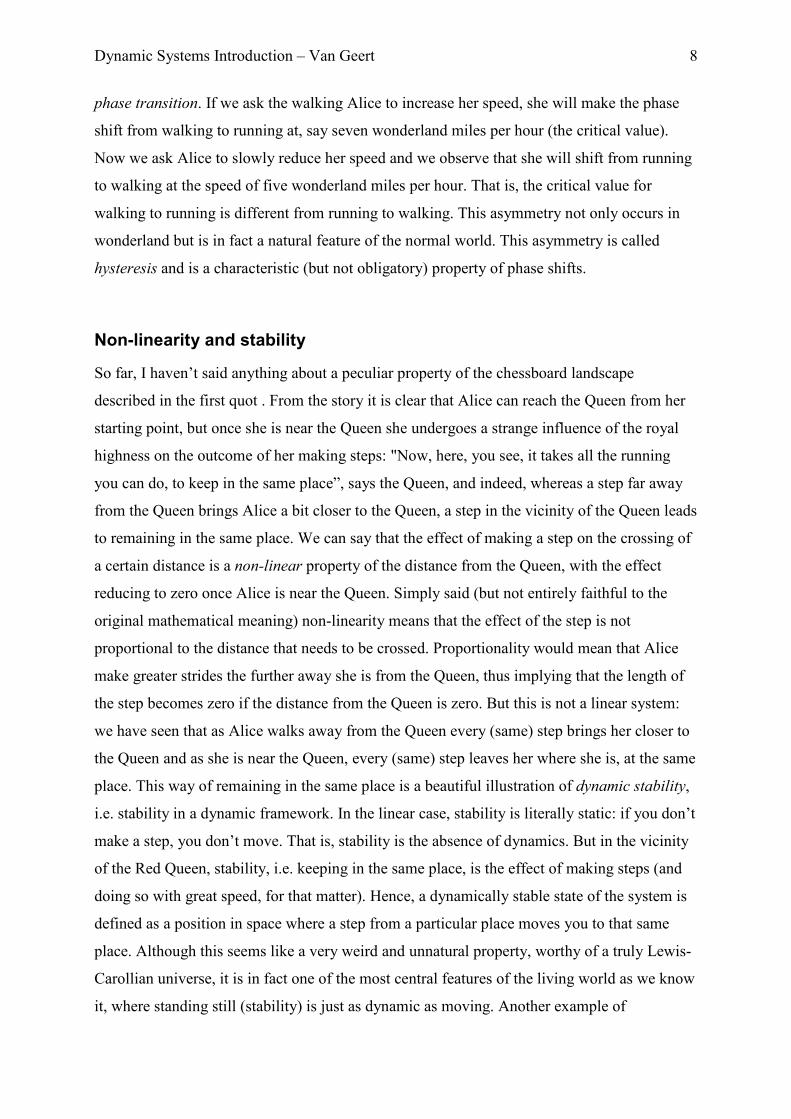
phase transition. If we ask the walking Alice to increase her speed, she will make the phase

shift from walking to running at, say seven wonderland miles per hour (the critical value).

Now we ask Alice to slowly reduce her speed and we observe that she will shift from running

to walking at the speed of five wonderland miles per hour. That is, the critical value for

walking to running is different from running to walking. This asymmetry not only occurs in

wonderland but is in fact a natural feature of the normal world. This asymmetry is called

hysteresis and is a characteristic (but not obligatory) property of phase shifts.

Non-linearity and stability

So far, I haven’t said anything about a peculiar property of the chessboard landscape

described in the first quot . From the story it is clear that Alice can reach the Queen from her

starting point, but once she is near the Queen she undergoes a strange influence of the royal

highness on the outcome of her making steps: "Now, here, you see, it takes all the running

you can do, to keep in the same place”, says the Queen, and indeed, whereas a step far away

from the Queen brings Alice a bit closer to the Queen, a step in the vicinity of the Queen leads

to remaining in the same place. We can say that the effect of making a step on the crossing of

a certain distance is a non-linear property of the distance from the Queen, with the effect

reducing to zero once Alice is near the Queen. Simply said (but not entirely faithful to the

original mathematical meaning) non-linearity means that the effect of the step is not

proportional to the distance that needs to be crossed. Proportionality would mean that Alice

make greater strides the further away she is from the Queen, thus implying that the length of

the step becomes zero if the distance from the Queen is zero. But this is not a linear system:

we have seen that as Alice walks away from the Queen every (same) step brings her closer to

the Queen and as she is near the Queen, every (same) step leaves her where she is, at the same

place. This way of remaining in the same place is a beautiful illustration of dynamic stability,

i.e. stability in a dynamic framework. In the linear case, stability is literally static: if you don’t

make a step, you don’t move. That is, stability is the absence of dynamics. But in the vicinity

of the Red Queen, stability, i.e. keeping in the same place, is the effect of making steps (and

doing so with great speed, for that matter). Hence, a dynamically stable state of the system is

defined as a position in space where a step from a particular place moves you to that same

place. Although this seems like a very weird and unnatural property, worthy of a truly Lewis-

Carollian universe, it is in fact one of the most central features of the living world as we know

it, where standing still (stability) is just as dynamic as moving. Another example of


nonlinearity is the hysteresis effect described in the preceding section: the critical value

depends on the direction from which you reach it.

Time scales

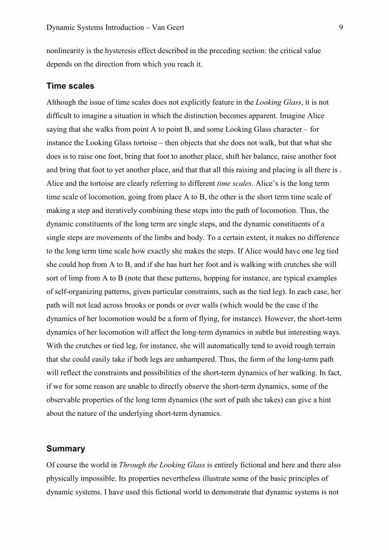
Although the issue of time scales does not explicitly feature in the Looking Glass, it is not

difficult to imagine a situation in which the distinction becomes apparent. Imagine Alice

saying that she walks from point A to point B, and some Looking Glass character – for

instance the Looking Glass tortoise – then objects that she does not walk, but that what she

does is to raise one foot, bring that foot to another place, shift her balance, raise another foot

and bring that foot to yet another place, and that that all this raising and placing is all there is .

Alice and the tortoise are clearly referring to different time scales. Alice’s is the long term

time scale of locomotion, going from place A to B, the other is the short term time scale of

making a step and iteratively combining these steps into the path of locomotion. Thus, the

dynamic constituents of the long term are single steps, and the dynamic constituents of a

single steps are movements of the limbs and body. To a certain extent, it makes no difference

to the long term time scale how exactly she makes the steps. If Alice would have one leg tied

she could hop from A to B, and if she has hurt her foot and is walking with crutches she will

sort of limp from A to B (note that these patterns, hopping for instance, are typical examples

of self-organizing patterns, given particular constraints, such as the tied leg). In each case, her

path will not lead across brooks or ponds or over walls (which would be the case if the

dynamics of her locomotion would be a form of flying, for instance). However, the short-term

dynamics of her locomotion will affect the long-term dynamics in subtle but interesting ways.

With the crutches or tied leg, for instance, she will automatically tend to avoid rough terrain

that she could easily take if both legs are unhampered. Thus, the form of the long-term path

will reflect the constraints and possibilities of the short-term dynamics of her walking. In fact,

if we for some reason are unable to directly observe the short-term dynamics, some of the

observable properties of the long term dynamics (the sort of path she takes) can give a hint

about the nature of the underlying short-term dynamics.

Summary

Of course the world in Through the Looking Glass is entirely fictional and here and there also

physically impossible. Its properties nevertheless illustrate some of the basic principles of

dynamic systems. I have used this fictional world to demonstrate that dynamic systems is not


a specific theory but that it is a general view on phenomena of whatever kind, with one basic

restriction, namely that they entail change. Concrete application of the principles and

properties illustrated by means of Alice’s adventures will of course depend on the actual part

of reality one wishes to observe and on particular choices the investigator needs to make in

order to keep the work manageable. In the next major section I will discuss some possible

applications of dynamic systems to the study of L2 acquisition, and where examples are not

available I will resort to illustrations from L1.

Dynamic systems and L2

Resolving a potential confusion

Dynamic systems already have a long history (see for instance Van Geert, 2005a for an

overview) and there is comparatively little disagreement in mathematics, physics or biology

what dynamic systems theory means. However, the situation is different for the

developmental sciences. If one searches the developmental literature on dynamic systems –

which is not extensive, but steadily increasing in terms of publications and fields of

application – one is likely to first run against publications that define dynamic systems theory

as a theory of embodied and embedded action (especially in the publications of Thelen and

Smith, see for instance Thelen and Smith, 1994 and Smith et al., 1999). In essence, cognition,

thinking and action are explained as dynamic patterns unfolding from the continuous, “here-

and-now” interaction between the person and the immediate environment. A particularly clear

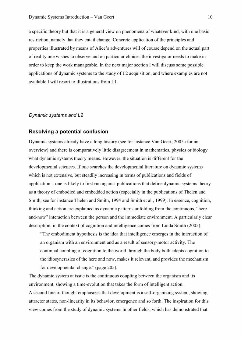
description, in the context of cognition and intelligence comes from Linda Smith (2005):

“The embodiment hypothesis is the idea that intelligence emerges in the interaction of

an organism with an environment and as a result of sensory-motor activity. The

continual coupling of cognition to the world through the body both adapts cognition to

the idiosyncrasies of the here and now, makes it relevant, and provides the mechanism

for developmental change.” (page 205).

The dynamic system at issue is the continuous coupling between the organism and its

environment, showing a time-evolution that takes the form of intelligent action.

A second line of thought emphasizes that development is a self-organizing system, showing

attractor states, non-linearity in its behavior, emergence and so forth. The inspiration for this

view comes from the study of dynamic systems in other fields, which has demonstrated that


such systems show the properties in question. An eloquent defender of this view is Marc

Lewis, who has primarily focused on social interaction, emotions and personality and,

recently, has shifted his attention to brain development (Lewis, 2000, Lewis, Lamey, and

Douglas, 1999; Lewis,1995; Lewis, 2005).

A third approach is the one that has been defended by the current author for about fifteen

years now, which is that dynamic systems is basically a very general approach to describing

and explaining change, focusing on the time evolution of some phenomenon of interest,

including the principles or “rules” that describe this time evolution (for general overviews, see

Van Geert, 1994, 2003 and Van Geert and Steenbeek, 2005; note that this entire overview of

names and publications is highly selective and that it does not do justice to many others who

have made contributions).

Fortunately, the differences in viewpoints are to a considerable extent only apparent (although

some points of disagreement remain, especially with regard to the way in which cognition or

language for that matter should be studied in a dynamic systems framework). If we apply the

general approach to systems that are complex and sufficiently permanent – such as human

beings, societies, but also more transient phenomena such as an action or a conversation – we

will soon find out that they display a host of interesting properties, namely emergence, self-

organization, attractor states, non-lnearity and so forth. Thus, the application of the general

approach to systems that are of interest, say, to students of second language acquisition, leads

to the second approach. The relationship with the first approach is a little more complicated

and requires some understanding of the concept of dynamics on various time scales, as

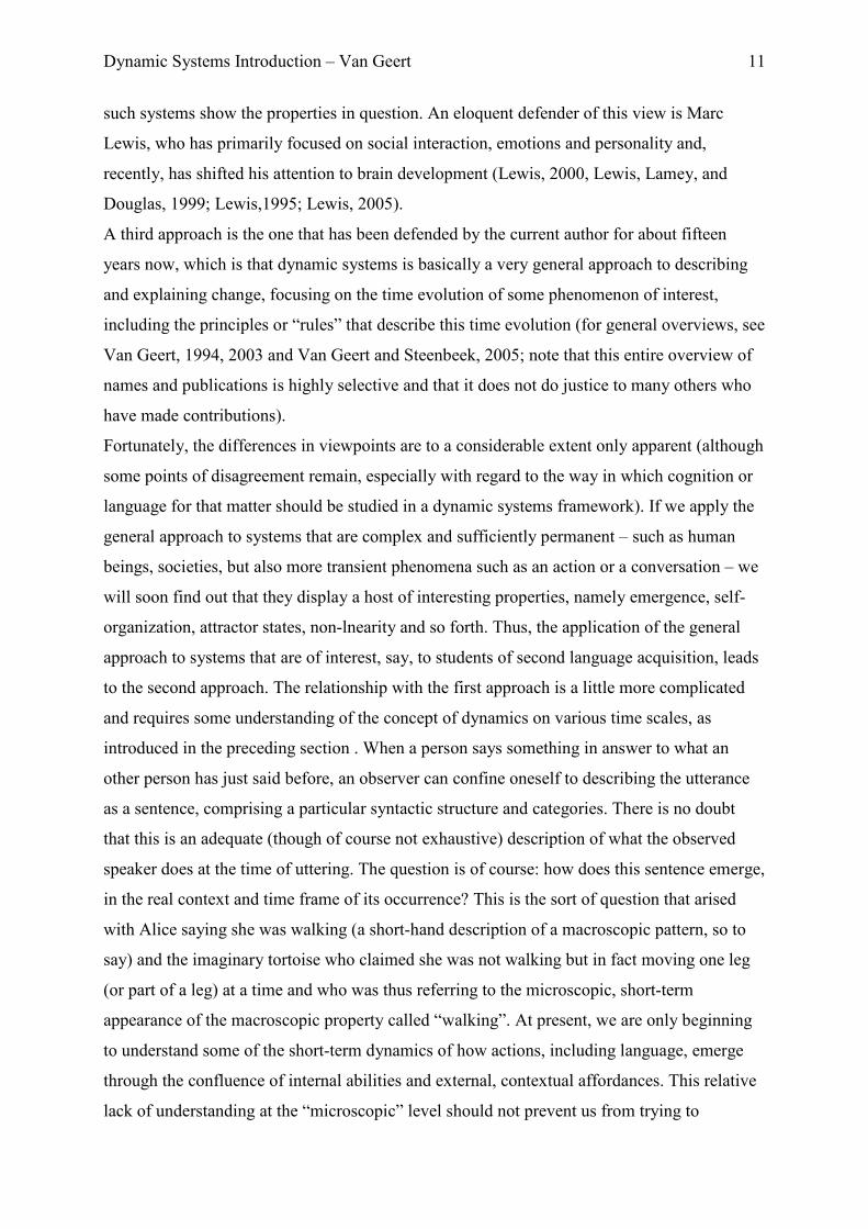
introduced in the preceding section . When a person says something in answer to what an

other person has just said before, an observer can confine oneself to describing the utterance

as a sentence, comprising a particular syntactic structure and categories. There is no doubt

that this is an adequate (though of course not exhaustive) description of what the observed

speaker does at the time of uttering. The question is of course: how does this sentence emerge,

in the real context and time frame of its occurrence? This is the sort of question that arised

with Alice saying she was walking (a short-hand description of a macroscopic pattern, so to

say) and the imaginary tortoise who claimed she was not walking but in fact moving one leg

(or part of a leg) at a time and who was thus referring to the microscopic, short-term

appearance of the macroscopic property called “walking”. At present, we are only beginning

to understand some of the short-term dynamics of how actions, including language, emerge

through the confluence of internal abilities and external, contextual affordances. This relative

lack of understanding at the “microscopic” level should not prevent us from trying to


understand the dynamics of a particular phenomenon, such as L2 learning, at the macroscopic

level of longer time frames (e.g. months or years during which the L2 is learned). However,

the short-term dynamics explaining the actual production an understanding of sentences on

the spot is characterized by a number of interesting properties, one of which is fluctuation and

variability (e.g. Thelen and Smith, 1994). These properties must be taken into account by any

model focusing on longer-term time scales and not be disregarded as, for instance,

measurement error. I will come back to this issue later.

In summary, the first approach to dynamic systems discussed in this section refers to a

particular, in general short-term time scale of the phenomena that can also be dealt with on the

long-term time scale of macroscopic change. However, the basic principles of dynamic

systems theory in the general sense must apply to all time scales (and this is the reason why

connectionist network models, which operate on the time scale of input-output relations in the

brain, are entirely compatible with dynamic systems principles and are thus examples of

dynamic systems, Pessa, 2004; Thelen and Bates, 2003).

Steps in the Construction of a dynamic system for L2

Searching for the state space description and the notion of order parameter

In its simplest possible form the acquisition of a second language, or a first language for that

matter, is a process that leads from a state of absence of any L2-specific linguistic proficiency

to a state (or collection of states) where proficiency of L2 is high enough to be interpreted as

“L2 has been acquired”. There is a lot more to say about this simplification, but let us

nevertheless take it as our starting point. From a UG point of view, one might object that even

if there is no apparent, observable expression of L2 or L1, there nevertheless is a lot of L1- or

L2-specific knowledge present in the form of UG. However, this remark does not exclude the

applicability of the principle that there is some – eventually arbitrarily chosen – initial state

and some final state, which need not be “initial and final” in any philosophical sense of the

word, but which simply mark the first and last state covered by a particular dynamic system

description. It goes without saying that the choice of the first and last state must make

empirical, theoretical or practical sense (e.g. as initial state one may take a student’s entry at a

particular L2-class and as final state the level after finishing the course, but this is of course

just one of the many possibilities).


Implicit in the above description is that individuals at any time of their life span can be rank-

ordered in terms of this proficiency. Hence, the proficiency dimension can be used as the state

space for the system in question, which in this case is a one-dimensional state space. Of

course one can easily object that L2-proficiency is in fact a summary of many aspects, such as

lexical knowledge, syntactic knowledge, fluency, pronunciation etc. and that there is no such

thing as L2-proficiency “tout court”. Be that as it may, but the central question is not if L2-

proficiency is the “real” state space for an L2-acquisition system. The question is: to what

extent does the reduction of the many degrees of freedom (incorporating lexicon, syntax etc.

etc.) to “proficiency” allow us to capture some of the theoretically and empirically relevant

aspects of the L2-acquisition dynamics?

To begin with, proficiency is a simple and yet powerful way of summarizing the many aspects

of a person’s familiarity with a language, and thus it serves as a macroscopic dimension along

which we can order the steps that a person takes on the path to L2-acquisition (and it also

serves as a ruler along which we can at least partially order various individuals in terms of L2

proficiency).

The choice of the state space dimension(s) reflects the organization of the system under

observation. A complex system (i.e. the sort of system we are interested in) shows a high

degree of organization, i.e. a high amount of coordination of its many components. In the case

of complex, developing and psychological systems, such as an L2-learner, this organization or

coordination is expressed in the form of a dominant or salient variable or category, the

application of which is often fuzzy but always very convenient. Take an example from a

different domain, namely an emotional expression, which is a combination of muscle

contractions in a person’s face, contextual elements and so forth, which are readily recognized

as, say, a smile (and not as a grin, or an angry face, etc.) Thus, the emotional expression is the

so-called order parameter of the facial, vocal and contextual system. This order parameter

specifies a number of distinguishable modes, the emotional expressions, which are separated

by fuzzy boundaries. An example from linguistics might refer to the distinction among

phonemes. Phoneme distinctions constitute an order parameter for the acoustic system. They

are categorically perceived, but separated by fuzzy boundaries, the fuzziness of which

depends, among others, on the fact that the underlying dimensions, such as voice onset time,

can be continuous). The order parameter must specify the most salient or distinguishable

aspect of a system’s behavior. It is clear that the choice of convenient state space dimensions

depends greatly on this notion of order parameter. That is, there is nothing that prevents us

from describing the L2-system of a person as a multi-dimensional space consisting of all


possible kinds of variables that are components of L2, whatever their nature. However, this

multi-dimensional description will often (but not necessarily always) just be too big, i.e. make

it very difficult for us to understand anything of the underlying dynamics. Hence, applying

dynamic systems to a complex phenomenon such as L2 amounts to trying to simplify the

system to its most salient or dominant mode, for the mere reason of making the dynamics

understandable. Psychologists tend to ask if such a dimension is “psychologically real”, which

they then try to answer by invoking results from basically correlational studies that present

associations between variables in populations. However, the question is whether such a

dimension is observationally adequate, or feasible, i.e. whether it suffices for us to see

essential features of an underlying dynamics (to the extent that a doctor is able to see essential

features of the dynamics of a person’s illness by plotting the person’s temperature over time,

without ever implying that the temperature and the illness are the same thing).

Whereas the emotions and phonemes examples refer to a form of categorical order parameter

(categories with fuzzy boundaries, thus suggesting certain continuities between the

categories), the hypothetical L2-proficiency order parameter is more easily represented as a

continuous order parameter, and thus, as a continuous state space dimension. Such

dimensions come close to the notion of a metric, let us say a ruler, along which the states of

the system can be measured in the classical sense of the word. In linguistics and psychology,

continuous order parameters are often represented in the form of tests providing a continuous

or quotient score (think about an intelligence test as a prime example). However, the test and

the state space dimension are not the same thing: they refer to each other, but it is not

necessary to have a test (e.g. of L2-proficiency) in order to fruitfully apply a particular state

space dimension or order parameter to a system (e.g. L2-proficiency as a convenient

descriptive construct). In some cases, the dimension or order parameter can be empirically

mapped onto a series of variables for which several tests are available, without implying that

the dynamics must be described by means of a state space with as many dimensions as there

are tests (or as many dimensions as there are factors in a factor analysis or principal

component analysis).

Static versus dynamic accounts of L2

In psychology, or any other science that deals with human behavior, including language, it is

customary to indirectly approach the dynamics of a phenomenon by finding out how the

distribution of a particular phenomenon in a group (population or sample) is related to


distributions of other phenomena in the group. For instance, one might wish to know the

association between a student’s oral performance on the one hand and the student’s task goal

orientation on the other hand. One can approach this question by taking a large sample of

students, measure their oral performance and goal orientation and calculate the correlation or

some other indicator of association, between the two measures, which, as we will find out,

takes a positive value. This association indicator is a so-called static measure (there is

absolutely no pejorative or evaluative meaning associated to that term), meaning that it

reflects the position of students in a group relative to each other (for a recent example relating

to adaptive language learning, see Woodrow, 2006, which appeared in this journal; note that I

am using this relationship as an example, about which I will speculate freely in order to try to

illuminate the difference between a static and a dynamic model; I am in no way claiming to

discuss or criticize Woodrow’s findings here). We can assume that the positive correlation

means that we will tend to find higher or better task orientation with students that have better

oral performance and, by definition, also the other way round. Technically, we can specify

this relationship as follows

yi = f(xi)

for y representing oral performance and x task orientation (or vice versa). The f stands for

function and means a positive association here, which allows us to predict a value for x, given

a value of y, within certain limits (the error term, or percentage explained variance).

However – and this is a very important point – the fact that an association holds over a

population or sample does not necessarily imply that such an association holds for a time

evolution or trajectory, i.e. a dynamic system. Thus, if we follow the time evolution of oral

performance and the time evolution of task orientation in a particular subject – which is where

the evolution takes place – we do not necessarily find that higher task orientation is related to

higher performance. This possible absence of positive relationship has nothing to do with

eventual random fluctuation or error. What I mean to say is that it is very well thinkable that a

static positive relationship over a population (including all kinds of error fluctuation) might

correspond with a negative dynamic relation (or anything else) in any or eventually all of the

individual members of the population. Think for instance – and this is purely speculative but

not impossible in my view – that a person’s goal orientation, including the strength of his

intention to perform well, invest more effort in accomplishing the task and so forth, increases

as the person perceives the task as more difficult and demanding, for instance reading and

understanding texts of high lexical and syntactic complexity. It is not unlikely that such

demanding tasks require the student to invest more effort in aspects other than oral


performance, and thus that the student’s oral performance in such tasks is on average lower

than in tasks that the student considers easy and not requiring a stronger task orientation than

the student is used to. Thus, seen in a dynamical perspective against the student’s own

standards of performance and perception of competence, the relationship between task

orientation and oral performance might be a negative one, whereas that same relationship is

positive if the topic of analysis is the sample of students.

The finding that a static relationship between two variables holding for a collection of

subjects (a sample) is not necessarily equal to the dynamic relationship between these

variables holding for each subject from the sample separately, is an example of the so-called

ergodicity problem, which statistical and methodological theorists in the humanities begin to

find increasingly interesting (See for instance Molenaar, 2004, for a particularly clear

example). The problem refers to the possible similarity of a space average (e.g. an average or

association or whatever) calculated for an ensemble of subjects, and a time average (i.e. an

average calculated over a sequence of steps in an individual). The speculative example of the

oral performance and task orientation relationship is an illustration of a situation in which this

similarity does not necessarily apply. Although this example is speculative, there exists

research in a different field that shows this inequality empirically. A study by Musher-

Eizenman, Nesselroade and Schmitz (2002) showed that the relation between perceived

control and academic performance found in a cross-sectional or classical longitudinal design

(few repeated measurements over a comparatively long time) was different from the relation

found when relatively short-term within-person change-patterns were studied. Thus, the short-

term dynamics of perceived control and academic performance in individuals is different from

the long-term or cross-sectional relationship. If this reasoning is applied to the oral

performance versus task orientation example, it would hold that whereas in the short run the

relationship between the two is negative, in the long run the relationship becomes positive

again, in that a long-term increase in goal orientation in an individual can be associated with a

long-term increase in that person’s oral performance (for an example of a distinction between

relationships holding over a sample and holding between time points in a dynamics of

language learning and instruction, see Van Geert and Steenbeek, 2005). .

Finding the evolution term and explaining the dynamics

In order to try to obtain a better understanding of this ergodicity problem and of the principles

of dynamics in general, consider the simplest possible format of a dynamic system, which is


yt+1 = f(yt) and xt+1 = g(xt)

which says that the next state (t+1) of a variable y or x is a function (f or g)of its preceding

state (t). If this is so, then any next state is a function of its preceding state, and the equation

produces a picture of the time evolution of y and x

yt → yt+1 → yt+2 → yt+3 → yt+4 → …. and xt → xt+1 → xt+2 → xt+3 → xt+4 → ….

which is a simple application of the iterativeness (or recursiveness) explained earlier. Thus,

the first question to answer is: what is the content of or the mechanism behind the enigmatic f

assuming that y represents L2-proficiency, i.e. the variable quality or level of L2 performance

of a person?. The simplest possible answer to this question is that, if L2-performance is part

of a learning-teaching process, the change of L2-performance is likely to be some form of

accretion, i.e. of adding some performance quality to the preceding state of L2-performance

quality. Earlier we have seen that an expression such as yt, say a person’s particular level of

language performance at time t, is in itself the result of a short-term dynamic process,

involving an intertwining of person and context characteristics. One consequence of this is

that performance, or y in general, will spontaneously fluctuate. Thus, the process of accretion

will be far from a neat linear increase and in fact will show the effect of the natural fluctuation

of performance. Since the fluctuation itself is a product of the underlying short-term dynamics

(e.g. the dynamics of sentence formation, or the dynamics of a conversation), the fluctuation

must not be treated as noise, i.e. as variability due to some independent, external source of

disturbance. Rather, the fluctuation, if properly described and understood, may contain

information about the underlying short-term dynamics and its effect on the long-term

dynamics of increasing L2-performance. For instance, in a study with Dominique Bassano,

we found that the pattern of sentence length during early L1-acquisition in two French-

speaking children showed two temporal increases in fluctuation magnitude. These variability

peaks coincided with rapid changes in the frequencies of holophrastic versus combinatorial

sentence constructions on the one hand and combinatorial versus typical syntactical

constructions on the other hand (the example will be discussed in more detail later, see

Bassano and Van Geert, in press). Another example, also in early L1-acquisition comes from

a study with Marijn van Dijk on variability peaks in the use of spatial prepositions, marking

the transition to rule-governed use of those preposition types in the child’s language (Van

Dijk and Van Geert, in press). Other examples of this phenomenon are presented in the article

by Lowie and Verspoor (this issue). In short, the theoretical specification of the evolution

term explaining the time evolution of L2-performance on the long term, will have to reckon

with the consequences of the short term dynamics, such as variability. These short term


dynamics are the subject of study of disciplines such as cognitive psychology (Costa, La Heij

and Navarrete, E., 2006) or neurocognition, or dynamic systems as defined by Thelen and

Smith (see for instance Colunga and Smith, 2006 and Jones and Smith, 2005, for an

application to word learning and use).

The accretion model of change in a context of teaching and learning, as in L2-learning

in a scholarly context, is likely to be too simplistic. Studies of learning of very different kinds

have shown that learning, i.e. the amount of increase of performance, skill or knowledge over

time, is proportional to the performance level already attained, proportional to the difference

between what is already learned and what has yet to be learned, and proportional to the

available resources (e.g. the quality of the teaching, the student’s motivation etc.). This

proportionality leads to various models of long-term change, the most likely or applicable of

which is the so-called logistic growth model, i.e. the model of growth under limited resources.

This dynamic growth model has been thoroughly explained elsewhere (Van Geert, 1991,

1996; De Bot, Lowie and Verspoor, 2006). Under ideal conditions, it leads to a smooth S-

shaped pattern of increase of performance, which stabilizes at a level it is able to maintain

given the available resources. For L2, those resources might imply the frequency with which

high-quality (native) L2 is heard by the L2-learner, the frequency of use, the speaker’s

linguistic talent (whatever that may mean) and so forth. However, as stated before, the

dynamic growth model must reckon with the properties of the short-term dynamics of actual

L2-production and L2-reception, which require explanation at a different time scale. As stated

before, a prime example of such a property is the natural fluctuation of performance over

time.

In the preceding section I discussed the example of oral performance and task

orientation, which demonstrated the importance of a particular coupling between variables.

Thus, task orientation is likely to affect oral performance over time, and we have seen that

this relationship need not be the same as the relationship found over a sample of subjects. The

relationship between variables relates to a particular property of dynamic systems, namely the

possibility to dynamically couple the variables in various ways. The formal format of a

coupled dynamic system is as follows

yt+1 = f(yt, xt) and xt+1 = g(xt, yt)

meaning that the next step of y depends on the preceding value of itself and of an other

variable, namely x, whereas the next step of x depends on its preceding value and the

preceding value of y.


In the simplest possible sort of model, the relationship between a variable and another can be

positive, as is the case if increased task orientation results in better oral performance, or

negative, as is the case if an increase in task orientation is due to perceived task difficulty

eventually resulting in lower performance than if the task is easy or less demanding. These

relationships are uni-directional, i.e. from one variable to another but not the other way

around.

More interesting dynamics result from mutual relationships between variables. Take for

instance the following speculative example. It is likely that in the early stages of L2-learning,

L2-use requires considerable effort, in that it is not yet a more or less automatic task and

requires monitoring, explicit attention and so forth. More effort will in principle result in

better performance (all other things being equal) and good performance, if it is recognized as

such by a more competent L2 conversation partner, will in principle help to maintain the

speaker’s motivation and thus the investment of effort. However, high levels of effort lead to

fatigue and fatigue is likely to affect performance negatively. Hence , the relationship between

performance and fatigue, via effort, is mutual but asymmetrical. It is positive from high

performance (via high effort) to fatigue in that high effort makes fatigue increase. It is

negative from fatigue to performance, in that higher fatigue results in lower performance. This

type of asymmetrical relationship, which can be compared to a predator-prey relationship, is

likely to produce oscillating patterns, i.e. waves of high performance and high fatigue (this is

of course an idealized example). However, the effort component depends clearly on the level

of mastery of L2. The more L2 usage becomes an automatic task performance, the less it will

appeal to the effort component and the less it will be a cause of fatigue. But fatigue from a

different source (e.g. a jet lag at the beginning of a conference) will still affect L2-

performance, even in an experienced L2-speaker. Thus, the nature of the dynamic

relationships changes over time and is also context- and origin-dependent.

To get back to the ergodicity problem and the issue of static versus dynamic models, assume

that a researcher has a sample of subjects at different levels of performance and at different

levels of effort required to achieve that performance. The relationship between performance

and fatigue over this sample will likely to be anomalous, that is, the correlation may be small

and statistically not significant. However, there is no direct link between this null-relationship

over the sample and the fatigue-performance relationships that govern the dynamics of L2-

acquisition and –performance in all the independent individuals forming the sample. In

individuals, the link is still present, and influencing the individual dynamics to a considerable


extent. However, the nature of the link itself is subject to developmental change and thus not

uniform over subjects.

Transitions in early language development: an example of dynamic

systems model building

A hypothetical model of three stages in early language acquisition

In a study carried out in collaboration with Dominique Bassano, an attempt was made to build

a dynamic model of long-term changes in language production, focusing on sentence length

as an indicator of underlying principles of first language production (for details see Bassano

and Van Geert, 2006). The model that we wished to check goes back to a hypothesis about

first language production that has been around for almost thirty years now. It assumes that, in

the construction of a genuine syntactic language, children begin with a stage in which one

word expresses a complex referential meaning (“holophrase”). The hypothesized generating

mechanism of language at this stage is therefore called the holophrastic generator. In a second

stage, the child is assumed to simply combine these complex holophrases into utterances

consisting of a few (two or three) such units, and thus generates language by means of

combination, hence the stage of the combinatorial generator. It is assumed that. while

combining words, children become sensitive to the way the language spoken by the linguistic

environment solves the combinatorial problem, which involves the use of syntax (order rules,

word correspondence etc.). Thus, the third and final stage in this respect is the stage at which

language is supposed to be based on a syntactic generator. These stages are assumed to occur

in the form of overlapping waves. The alternative hypothesis is that language development is

a continuous process (whatever the exact nature of the underlying continuous processes).

Data and method

The main set of data used in this study came from the longitudinal corpus of one French girl,

Pauline, who was studied from ages 1;2 to 3;0. Additional data are from another French child,

Benjamin, who was studied from age 2;0 to 3;0 (see for analyses of the children’s language

development Bassano, 1996). Data were obtained using a free speech sampling method. For

each child, frequencies of one-word, two-words, three words utterances, etc. (, W2, W3, etc.)

were calculated, for each monthly sample (120 utterances) and for the sub-samples (60


utterances and 30 utterances respectively). Figure 1 shows the smoothed curves of the raw

data, based on a Loess smoothing procedure (locally-weighted least-squares smoothing),

which provides a representation of the changes in the sentence frequencies and is able to

capture eventual temporal regressions, accelerations in the growth rate etc.

Insert Figure 1 about here

A dynamic model of stepwise grammatical development

The aim of this model is to explain the quantitative evolution of three types of utterances or

phrases, namely one-word, two-and-three-word and four-word-and-more phrases, called W1,

W23 and W4+ respectively. These types of phrases are supposed to be linked with the

linguistic generators described above. Before proceeding with the model, two remarks should

be made. The first is that the relationship between a particular type of phrase, for instance W1,

and its assumed underlying generator, is in itself a transient relationship, i.e. it changes over

developmental time. Thus, an early W1 is considered a product of the holophrastic generator,

but a late W1, occurring in the midst of W23 and W4+ phrases, is most likely an expression

of the assumed syntactic generator. This changing relationship must be taken into account

when interpreting the meaning of the linguistic data. Second, the model we wish to build does

not explain the emergence of a new generator out of an old one. In order to do so, a different

type of model would be required, showing how a procedure of word combination, for

instance, grows out of a procedure of using holophrases. Moreover, the model – which is a

model of long-term change – does also not intend to explain the short-term dynamics of

phrase production, for instance it does not provide an explanation of how and why children, in

their actual speech producing processes, make a choice between a holophrastic and

combinatorial generator at developmental stages when both are available.

The term “ explain” might give rise to confusion. Of course, the dynamic model might be

said to “explain” this choice by invoking the notion of a random selection between two

available generators, given the expected frequencies at some particular moment in time.

However, this model-theoretic random selection is not intended as a literal description of the

actual short-term process of phrase production and does not in itself imply that a language-

producing child literally makes a stochastic response choice. In fact, for reasons of simplicity,

the long-term model treats the short-term process as if it where a stochastic choice as

convenient for the time being and leaves the description of how the process actually occurs on


the short-term of phrase production to a theory and design that studies this short-term time

scale directly.

In line with comparable growth models of long-term change, we postulated that the

hypothesized generators – which are hierarchically ordered in terms of assumed

developmental complexity and order – were characterized by bi-directional asymmetric

relationships (see figure 2).

Insert figure 2 about here

Relationships run from the less to the more advanced generator and from the more to the less

advanced.

First, the relationships from the less advanced to the more advanced generator are supportive

and conditional. For instance, the holophrastic generator explains the increase in the

production of one-word phrases. It is assumed that a minimal level of one-word phrase

production is necessary to make the transition to a combinatorial grammar, which generates

two- and three-word phrases. This minimal required level or critical mass is needed for the

combinatorial generator to emerge, hence the notion of a conditional relationship from

holophrastic to combinatorial generator. The supportive relationship between holophrastic to

combinatorial generator implies that there is a linear, positive relationship between the

number of W1-phrases actually produced and the increase in the number of W23-phrases.

That is, “simpler” formats such as W1- phrases produced by a holophrastic generator are

assumed to stimulate the production of more complex formats, such as W23-phrases produced

by a combinatorial generator. I see this as a very simple, but basic developmental assumption,

which can be explained on the basis of classical developmental and learning theoretical rules

or principles (see Van Geert, 1998b).

Second, the relationships from the more advanced to the less advanced generator are

competitive. This relationship implies that the more the more advanced generator is used, the

less the less advanced generator will be used and the more it will decline. The reasons for this

relationship are diverse. For instance, the more advanced generator is likely to produce

phrases that are more similar to the linguistic input as the child perceives the latter, or are

more similar to the phrase that the other speakers produce in response to the child, etc. (see

for instance MacWhinney, 1998).

The competitive relationship is, in all likelihood, a transitive relationship. That is, it holds for

all generators that are less complex or less mature. Thus, a competitive relationship from the

syntactic to the combinatorial generator implies also a competitive relationship from the

syntactic to the still older holophrastic generator.


The next step is to specify a mathematical model that provides a formal representation of the

set of relationships. For instance, the supportive relationship entails a positive effect of the

productivity of a more mature generator on a less mature one. Thus, if Ct represents the

frequency of W23 at time t and St represents the frequency of W4+ phrases at time t, the

increase in St, which we can write as ∆S/∆t, is proportional to Ct, and thus, if the parameter d

stands for that proportion, ∆S/∆t depends on d* Ct (for * the multiplication symbol). In one of

the preceding sections, we have seen that the effect of a growth factor or learning factor on a

variable, is likely to be proportional to the current level of that variable. That is, the

magnitude of the effect of C on S is proportional to the current level of S. If e is a parameter

that stands for that particular proportion, we can now combine the two effects in a simple

equation that specifies the effect of C of S, as follows

∆S/∆t = d* Ct * e * St

If, for simplicity, we set d * e equal to a value c, we find that

∆S/∆t = c* Ct * St

which is the expression for a supportive relationship. If c takes a negative value, the equation

expresses a competitive relationship.

It can be shown that growth and learning processes are processes of limited increase (see Van

Geert, 1991). A trivial example of a limitation is the amount of time a person can spend

producing phrases (which is certainly limited by a person’s life span). A less trivial example,

relating to growth of the lexicon, is that such growth is limited by the number of words

available in the language. This reasoning leads to the following model, which, for simplicity

will be applied to the increase, over time, of the number of W1-phrases uttered by a child, for

instance on an average day. Given that a child must, logically, begin with one word that is its

first, the number of one-word phrases, represented by H for holophrases, will grow over time,

and this growth is, as we have seen, most likely proportional to the level of H already

attained. Thus, the increase of H, ∆H/∆t = b* Ht , for b a proportion that specifies the rate of

increase. However, we have just stated that increase is limited. The simplest way of

specifying this limitation is that b, the rate of increase, will decrease as H gets bigger and thus

approaches its limitations, and this decrease is proportional to H (let us say the symbol a


represents this proportion). This verbally stated relationship can be expressed in mathematical

format in the following way

∆H/∆t = ( b - a* Ht )* Ht

We have also stated that H “suffers” from the increase of more complex phrases, based on the

combinatorial generator. Thus, the increase in H over some time t can be expressed as follows

∆H/∆t = ( b - a* Ht )* Ht - g* Ct * Ht

Applying a comparable logic to the growth of W23 (the C-generator utterances) and W4+ (the

S-generator utterances), we arrive at the following coupled dynamic system

∆H/∆t = ( b - a* Ht )* Ht - g* Ct * Ht - h* St * Ht

∆C/∆t = ( i - j* Ct )* Ct + k* Ht * Ct - l* St * Ct

∆S/∆t = ( m - n* St )* St + s* Ct * St

which describes the time evolution of W1, W23 and W4+ phrases (remember that the

connection between a type of phrase and a generator, e.g. W1 and the H-generator, changes

over time, which makes the connection between the model and the empirical data more

complicated). This is a dynamic system described by a three-dimensional state space (the H,

C and S dimension). For simplicity, it can be represented by three separate one-dimensional

time evolutions (the time evolution of H, C and S separately).

Mathematically, this model is equivalent to the following notation (for reasons of simplicity

and without loss of generality, we can confine ourselves to the H-variable):

Ht+1 = Ht + b * (1 – Ht / KH) - g* Ct * Ht - h* St * Ht

for KH the limit level of H (the highest possible level H can attain under the present limiting

circumstances). This K-parameter has an interesting property: since the limit level, specified

by K, is a function of all the available resources, whether they be internal or external, K

amounts to a single-value representation of all the available resources. The fact it is at all

possible to represent the very complex structure of resources (memory, effort, help given,

motivation, talent, available books, etc. etc. …) by a single value is a direct consequence of


the fact that the resources are represented in function of the dynamic effect they have on the

growth and stabilization of the variable at issue (H in this case).

Finally, the coupled-dynamics model specifies only the supportive and competitive

relationships, not the conditional relationships which have been left out from the above

equations to avoid further complication. They can be added to the equations in the following

way (the example is limited to the C-component):

∆C/∆t = 0 if Ht < HP

∆C/∆t = ( i - j* Ct )* Ct + k* Ht * Ct - l* St * Ct if Ht ≥ HP

for HP the conditional value H must have for C to grow.

The next question is of course what the value of these a, b … parameters should be. They can

be estimated by mere guessing and then trying out the model with these guessed values to see

whether it fits the data. However, they can also be estimated by means of parameter

optimization programs that calculate the best possible set of parameters, i.e. the set for which

the model produces the best possible fit with the data. Since the W23 and W1 phrases

occurring later in developmental time are “ absorbed” by the emerging syntactic generator

(thus meaning that a late W1 is produced by the S-generator, and no longer by the original H-

generator, for instance), the data must be rescaled in order to account for this absorption

process. This rescaling was done by normalizing the data to values between 0 and 1 and by

subtracting a baseline value. Figure 3 shows the result of this optimization procedure,

showing that the model provides a good fit with the normalized and rescaled data.

Insert figure 3 about here

Evidence of stage transitions?

The dynamic model predicts that the probabilities of W1, W23 and W4+ sentences increase

an decrease in a smooth way. For instance, every day the expected frequency of W1 phrases

decreases a little bit, whereas the expected frequency of the W23 gradually increases. This

means that for any episode of language production long enough to arrive at reliable frequency

counts – say an episode of a couple of hours or days maybe – the expected frequencies will

change smoothly. Since the observed frequencies depend on the expected frequencies, which

are in fact probabilities of production, the observed frequencies will of course fluctuate over

days or hours. These fluctuations must be within the bounds predicted by the probabilities of

production, represented by the smoothed frequencies which the dynamic model so nicely


simulates. So far, all this is an expression of an orderly world. However, we began this article

by visiting Alice’s Looking Glass, and so we will end. Thus, it is time to imagine some weird

events.

Just assume that around the age of 22 months, Pauline produces only W1-phrases on even

calendar days and only W23-phrases on uneven calendar days. Thus, in a truly Alicean way,

it’s either Holophrase or Combinatorics for Pauline (around the age of 22 months, that is,

things might change afterwards). That is, the two generators are in harsh competition, and

there is an age (e.g. 22 months) where both have the same chance to win the contest and thus

to determine the sort of phrases that will be uttered during a particular day. If this were so, we

would observe a maximal fluctuation over days between 100% W1 and 100% W23 for some

time. This day-to-day fluctuation will thus be considerably greater than the fluctuation we

expect to find if the generators wax and wane in the smooth way of the dynamic model, which

so nicely fits the smoothed data. However, this condition of increased fluctuation is less

“through-the-looking-glass”-like as one might expect. In fact, increased fluctuation was

exactly what we found in Pauline’s and Benjamin’s data. We found two periods of fluctuation

were the variability was significantly greater than should be expected on statistical grounds,

given the observed probabilities of the three phrase types (details can be found in Bassano and

Van Geert, 2006-in press). What this finding means is that reality lies somewhere between the

continuous dynamic model and the discontinuous world inspired by the looking-glass magic.

That is, as a new generator emerges, there is a short period during which the child feels

(moderately) “torn between two generators”, and this is the kind of thing one expects to find

during true developmental transitions (see for instance Ruhland and van Geert, 1998, for an

application of catastrophe theory to language development). To put it differently, the study of

fluctuations and intra-individual variability may add to our understanding of the underlying

developmental processes, which testify both of continuity and gradualness on the one hand

and discontinuity and transition on the other hand (see Van Dijk and Van Geert, 2006 – in

press).

Conclusion

In the current example of L1-learning I have discussed the possibilities and limitations of a

dynamic systems approach to language development. These principles are not limited to early

language acquisition but are general enough to apply to L1 as well as L2, spontaneous as well

as formalized scholarly learning, learning and acquisition as well as language loss and


deterioration of a language(for an application to L2-learning, see de Bot, Lowie and Verspoor,

2006-in press). As the reader will have noticed, there are various ways in which dynamic

systems theory can be applied to language learning and acquisition, there are different time

scales and phenomena to be explained, one can resort to making mathematical models or to

detailed analysis of fluctuations in the data. These possibilities do still not exhaust the

richness of this approach. It must be emphasized that it is not an approach that allows for

simple general answers and there is so much that has yet to be explored and tried out. It is not

an approach that aims to abandon and pretends to be a replacement for the current, established

way of studying language growth, learning and change. However, the view of dynamic

systems is crucial if we want to go beyond the static or structural relationships between

properties or variables and wish to understand the mechanism of development and learning as

it applies to individual persons. The road towards an understanding of the dynamics of L1-

and L2-acquisition and learning is steep and long and paved with difficulties, but it is a road

well worth taking.

References

Bassano, D. (1996). Functional and formal constraints on the emergence of epistemic

modality: A longitudinal study on French. First Language, 16, 77-113.

Bassano, D. and Van Geert, P. (2006). Modeling Continuity and Discontinuity in

Utterance Length: A quantitative approach to changes, transitions and intra-individual

variability in early grammatical development. Developmental Science, in press.

Bates, E. & Goodman, J. C. (1997). On the inseparability of grammar and the lexicon:

Evidence from acquisition, aphasia, and real-time processing. Language and Cognitive

Processes, 12, 507-584.

Colunga, E., & Smith, L. B. (2005). From the lexicon to expectations about kinds: A

role for associative learning. Psychological Review, 112, 347–382.

Costa, A., La Heij, W and Navarrete, E. (2006). The dynamics of bilingual lexical

access. Bilingualism: Language and Cognition 9 (2), 2006, 137–151.


De Bot, K, Lowie, W. and Verspoor, M. (2006). A Dynamic Systems Theory

Approach to Second Language Acquisition. Bilingualism, 9, in press.

Jones, S. S., & Smith, L. B. (2005). Object name learning and object perception: A

deficit in late talkers. Journal of Child Language, 32, 223–240.

Lewis, M. D. (1995). Cognition-emotion feedback and the self-organization of

developmental paths. Human Development, 38, 71-102.

Lewis, M. D. (2000). The promise of dynamic systems approaches for an integrated

account of human development. Child Development, 71, 36-43.

Lewis, M. D. (2005). Self-organizing individual differences in brain development.

Developmental Review, 25, 252-277.

Lewis, M. D., Lamey, A. V., & Douglas, L. (1999). A new dynamic systems method

for the analysis of early socioemotional development. Developmental Science, 2, 457-475.

MacWhinney, B. (1998). Models of the emergence of language. Annual Review of

Psychology, 49, 199-227.

Molenaar, P. C. M. (2004). A Manifesto on Psychology as Idiographic Science:

Bringing the Person Back Into Scientific Psychology, This Time Forever. Measurement:

Interdisciplinary Research & Perspectives, 2, 201-218.

Musher-Eizenman, D. R., Nesselroade, J. R., & Schmitz, B. (2002). Perceived control

and academic performance: a comparison of high- and low-performing children on within-

person change-patterns. International Journal of Behavioral Development, 26, 540-547.

Pessa, E. (2004). Quantum connectionism and the emergence of cognition. In

G.G.Globus, K. H. Pribram, & G. Vitiello (Eds.), Brain and being: At the boundary between

science, philosophy, language and arts (pp. 127-145). Amsterdam (NL): John Benjamins

Publishing Company.

Ruhland, R. & van Geert, P. (1998). Jumping into syntax: Transitions in the

development of closed class words. British Journal of Developmental Psychology, 16, 65-95.

Smith, L. B., Thelen, E., Titzer, R., & McLin, D. (1999). Knowing in the context of

acting: The task dynamics of the A-not-B error. Psychological Review, 106, 235-260.

Thelen, E. & Bates, E. (2003). Connectionism and dynamic systems: are they really

different? Developmental Science, 6, 378-391.

Smith, L. B. (2005). Cognition as a dynamic system: Principles from embodiment.

Developmental Review, 25, 278-298.

Thelen, E. & Smith, L. B. (1994). A dynamic systems approach to the development of

cognition and action. Cambridge (MA): Bradford Books/MIT Press.


Van Dijk, M and Van Geert, P. (2006). Wobbles, Humps and Sudden Jumps: A Case

Study of Continuity, Discontinuity and Variability in Early Language Development, Infant

and Child Development, 15, in press.

Van Geert, P. (1991). A dynamic systems model of cognitive and language growth.

Psychological Review, 98, 3-53

van Geert, P. (1998a). We almost had a great future behind us: The contribution of

non-linear dynamics to developmental-science-in-the-making. Developmental Science, 1,

143-159.

Van Geert, P. (1998b). A dynamic systems model of basic developmental

mechanisms: Piaget, Vygotsky and beyond. Psychological Review, 105, Vol. 5, No. 4, 634–

677

Van Geert, P. (2003). Dynamic systems approaches and modeling of developmental

processes. In J. Valsiner and K. J. Conolly (Eds.), Handbook of developmental Psychology.

London: Sage. Pp. 640-672.

Van Geert, P. and Steenbeek, H. (2005). Explaining after by before. Basic aspects of a

dynamic systems approach to the study of development. Developmental Review, 25 (3-4),

408-442.

Woodrow, L.J. (2006). A Model of Adaptive Language Learning. The Modern

Language Journal, 90, 297- 319.

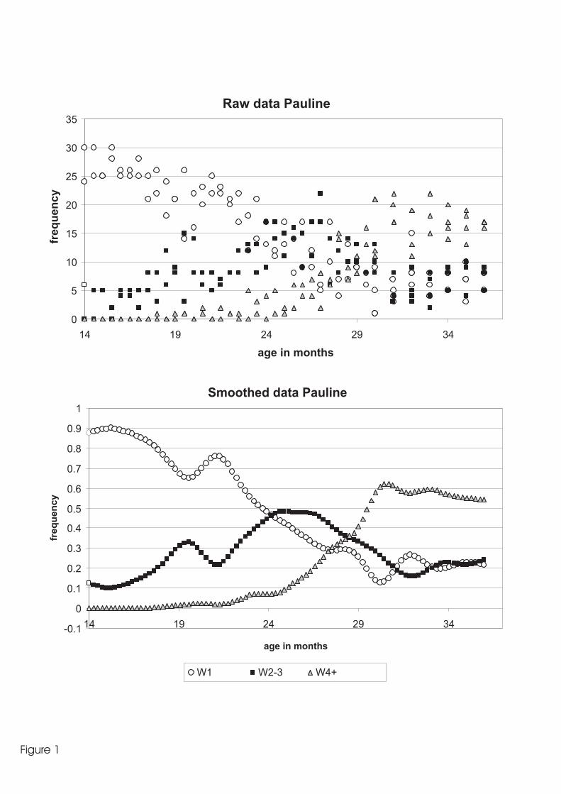
Raw data Pauline

0

5

10

15

20

25

30

35

14 19 24 29 34

age in months

fre

qu

en

cy

Figure 1

Smoothed data Pauline

-0.1

0

0.1

0.2

0.3

0.4

0.5

0.6

0.7

0.8

0.9

1

14 19 24 29 34

age in months

fre

qu

en

cy

W1 W2-3 W4+

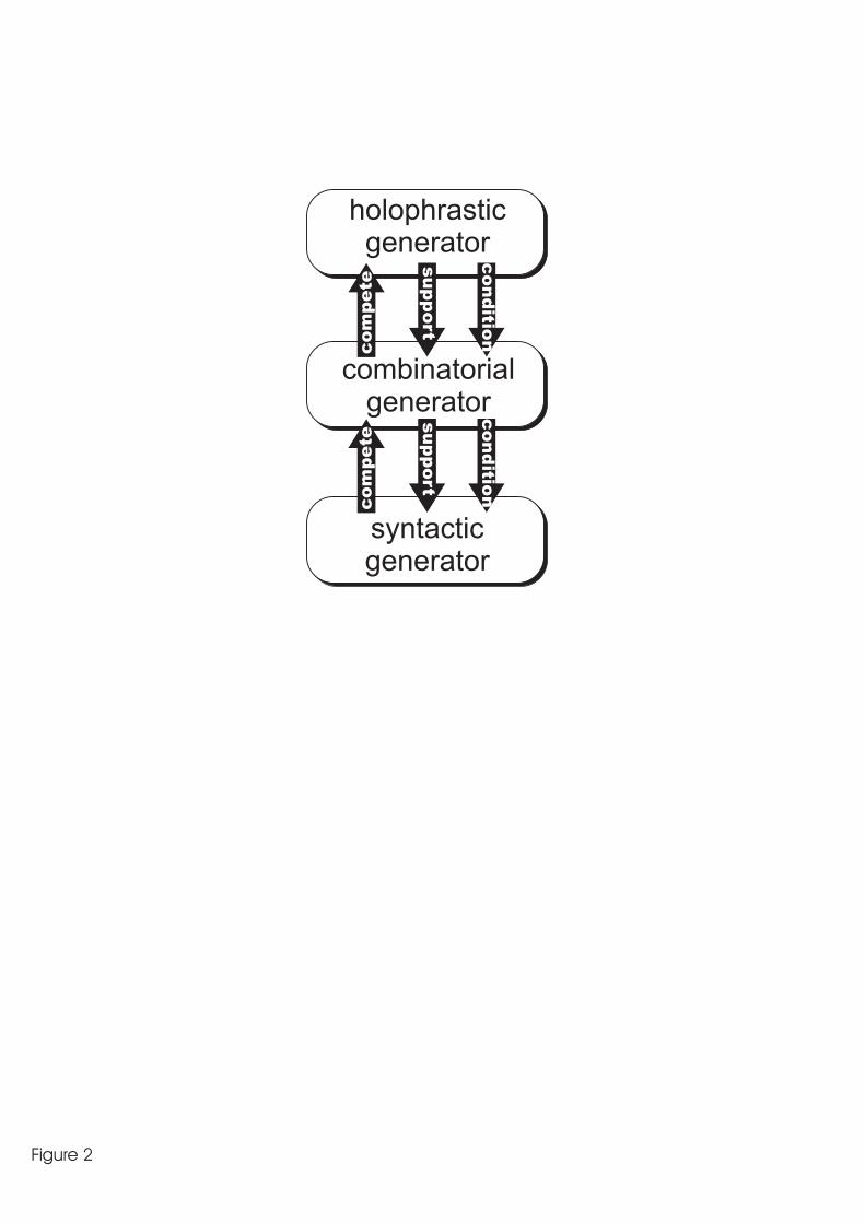
holophrasticgenerator

combinatorialgenerator

support

conditio

ncom

pete

syntacticgenerator

support

conditio

ncom

pete

Figure 2

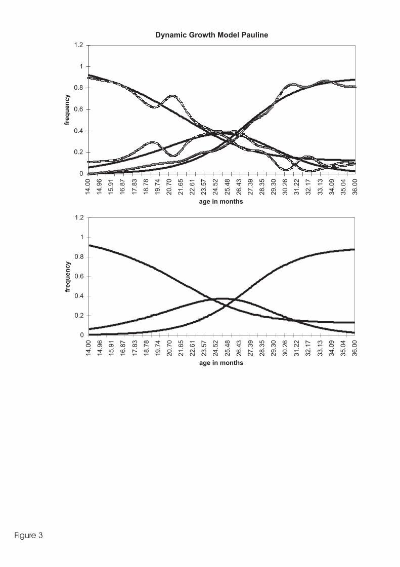
Dynamic Growth Model Pauline

0

0.2

0.4

0.6

0.8

1

1.2

14.0

0

14.9

6

15.9

1

16.8

7

17.8

3

18.7

8

19.7

4

20.7

0

21.6

5

22.6

1

23.5

7

24.5

2

25.4

8

26.4

3

27.3

9

28.3

5

29.3

0

30.2

6

31.2

2

32.1

7

33.1

3

34.0

9

35.0

4

36.0

0

age in months

freq

uen

cy

0

0.2

0.4

0.6

0.8

1

1.2

14.0

0

14.9

6

15.9

1

16.8

7

17.8

3

18.7

8

19.7

4

20.7

0

21.6

5

22.6

1

23.5

7

24.5

2

25.4

8

26.4

3

27.3

9

28.3

5

29.3

0

30.2

6

31.2

2

32.1

7

33.1

3

34.0

9

35.0

4

36.0

0

age in months

freq

uen

cy

Figure 3

Documents

The Dynamic Systems approach in the study of L1 and L2 acquisition