Embed Size (px)
Citation preview

Faculté des sciences économiques
et de gestion
PEGE 61, avenue de la Forêt Noire
67085 STRASBOURG Cedex Tél. : (33) 03 90 24 21 52 Fax : (33) 03 90 24 20 64
www-ulp.u-strasbg.fr/large
Institut d’Etudes Politiques 47, avenue de la Forêt Noire
67082 STRASBOURG Cedex
Laboratoire de Recherche
en Gestion & Economie
LARGELARGE
PapierPapiern° 2008-09
Are French Individual Investors reluctant to realize their losses ?
Shaneera Boolell-Gunesh / Marie-Hélène Broihanne / Maxime Merli
Avril 2008
1
Are French Individual Investors reluctant to realize their losses?
Boolell-Gunesh. S1 – Broihanne M-H2. – Merli M. January 2009
Abstract
We investigate the presence of the disposition effect for 90 244 individual investors using a unique large brokerage account database between 1999 and 2006. Our main results show that individual investors demonstrate a strong preference for realizing their winning stocks rather than their losing ones. However, the fiscal impact in France appears to be moderate relative to the one observed in other countries. Taking French specificities such as, the way short sales are realized and the existence of tax free account (PEA account) into account, show that: a) the behavioral bias is not eliminated for sophisticated individual investors; b) the change of “tax account type” does not imply any change in investors’ behavior JEL Classification : G 10
Résumé
Nous étudions la présence d’un effet de disposition pour 90 244 investisseurs individuels français à partir d’une base de données de transactions individuelles sur la période 1999-2006. Les principaux résultats montrent que ces investisseurs ont une préférence marquée pour la réalisation de leurs gains plutôt que de leurs pertes. L’impact fiscal semble en France plus modéré que dans d’autres pays En outre, l’existence de possibilités de ventes à découvert (SRD) et de comptes PEA en France permet de mettre en lumière de façon originale a) la persistance de ce biais pour des investisseurs sophistiqués et b) le faible impact du régime fiscal sur le comportement des investisseurs.
1Corresponding author : LaRGE / EM Strasbourg Business School, Strasbourg University, 61 avenue de la forêt noire, 67085 Strasbourg Cedex, France. E-mail :
JEL Classification : G 10
[email protected] 2 LaRGE / EM Strasbourg Business School, Strasbourg University E-mail: [email protected]/ [email protected].
2
I-Introduction Recent research in behavioral finance has demonstrated that investment behavior is not
always consistent with the assumptions of perfect rationality generally made in the field.
More precisely, this behavior has sometimes been shown to be systematically different from
what is implied by normative models of standard finance theory.
One of the most widely documented behavioral biases is the disposition effect. This effect
describes the tendency, at any given point in time, to more readily sell winners than losers,
winners and losers referring to assets that have appreciated or depreciated since purchase. In
this framework, researchers have shown that investors who are prone to the bias earn poor
subsequent returns on their portfolio (Odean, 1998). Of course, rational reasons can justify
this behavior: portfolio rebalancing or higher trading costs of low priced assets, for instance.
However, none of these reasons has been found convincing enough by researchers.
Starting with Shefrin and Statman (1985), a number of researchers among others have
documented the effect: Lakonishok and Smidt (1986) on aggregate volumes, Odean (1998),
Shapira and Venezia (2001), Dhar and Zhu (2006) on individual data3
Our paper fits this loophole by investigating the trading records of 90 244 individual investors
at a French discount brokerage house between 1999 and 2006. As a result, the first
contribution of this study is to be the first one on the French market and the most
comprehensive in the European context
.
However, if the presence of the disposition effect has been answered in some countries, no
such research has yet been carried out in France.
4
3 Note that Weber and Camerer (1998) and Weber and Welfens (2006) bring experimental evidence of this biais. 4 The only European research dealing with the disposition effect on individual data concerns 3 079 accounts (Weber and Welfens, 2006).
. We find that investors show a strong preference for

3
realizing paper gains rather than their paper losses and that this behavior cannot be explained,
for instance, by a desire to rebalance portfolios.
We expect some investors to be more sophisticated than others. To be precise, investors are
ranked as sophisticated ones if they trade derivative assets, internationally diversify their
portfolio or use short selling facilities (French SRD). Based on this original approach, our
second contribution demonstrates that sophisticated traders are also subject to the bias which
leads us to conclude that sophistication attenuates but does not eliminate the disposition
effect.
At the aggregate level, we show that the impact of the tax year effect is clearly less important
in France than in other countries. French specificities i.e the existence of PEA account (Plan
d'Epargne en Actions) give a unique opportunity to investigate more deeply the global impact
of tax on the selling behavior of investors on the financial market. Actually, these accounts
offer an interesting tax framework to their holders in the sense that capital gains are tax free if
the account has been kept for more than 5 years. In this framework, we study the disposition
effect for holders of PEA accounts before and after the end of the 5-year period. We show that
individual investors do not seem to change their investment behavior according to the type of
fiscal account held (PEA or traditional). This original is our third important contribution.
The rest of the article is organized as follows. The second section presents an overview of
previous research on the disposition effect. Section III describes the data and introduces the
methodology. Section IV is dedicated to the description of our main results and comments and
finally we conclude in section V.

4
II-The Disposition Effect
The disposition effect is the tendency of investors to hold losers (losing stocks) too long and
sell winners (winning stocks) too soon. This phenomenon was first documented by Shefrin
and Statman (1985) in a study of mutual fund performance. Subsequent papers based on
market data (Lakonishok and Smidt, 1986; Ferris, Haugen and Makhija, 1988) showed that
volume for winning stocks on the NYSE and the Amex exceeds that for losers.
From a theoretical point of view5, many explanations of the disposition effect have been
proposed in the literature. The most common explanation is based on the assumption of
prospect theory preferences (Tversky and Kahneman, 1979, Kahneman and Tversky 1992)
and, more precisely, on the S-shaped valuation function assumed in this model. According to
this theory, investors evaluate gains and losses with respect to a reference point; the buying
price is the most commonly used reference point. When a stock price is higher than the
buying price (or more generally than the reference price), the investor is in the concave part of
his valuation function and is hence risk averse. He may sell the stock if the expected return is
perceived as too low. After a price drop, the investor is in the convex part and keeps the stock
because he has become risk seeking. Following Shefrin and Statman (1985), some authors
have used this argument to justify the existence of disposition investors (Odean (1998) and
Weber and Camerer (1998), for example). In other words, when agents are risk-averse over
gains and risk lovers over losses, they prefer to realize paper gains and to keep paper losses6
5 For experimental studies of this bias, see for example, Weber and Camerer (1998), Chui (2001), Weber and Welfens (2006) and Rubaltelli et al. (2005). 6 Barberis and Xiong (2006) (see also Hens and Vlcek (2005)) show that the disposition effect is observed for some values of the expected stock return and the horizon of the investor, but they also find the opposite effect for other reasonable values of these parameters. Note that Barberis and Xiong (2008) give some new theoretical explanation of the disposition effect based on a “realization utility”.
.
5
A second explanation is based on an irrational belief in mean reversion of stock prices, which
states that investors believe poorer-performing stocks will rebound, and that better-performing
stocks will decline in price. Briefly speaking, after a price increase, the investor believes that
the probability of a price drop in the next period is higher than the one of another price
increase (Shu et al. (2005), Weber and Camerer (1998)).
A third group of explanations argue that the disposition effect may be due to the desire to
rebalance portfolios or to avoid higher transactions costs on low-priced assets. However, it
has been shown in many studies that when controlling for rebalancing and share prices, the
disposition effect is still observed and that the investments the investors choose to sell
continue in subsequent months to outperform the losers they keep (see Odean (1998), Brown
et al. (2006), for example).
A last explanation of the disposition effect is proposed by psychologists who work on the
theory of entrapment or escalation of commitment (Staw (1979), Brockner (1992)). In an
investment context, the question is to know if it is better to keep a losing investment, to
increase the stake (to break even), or to sell the losers and choose other stocks to invest in
(Zuchel, 2001).
Finally, the disposition effect can also refer to preferences, including the idea that investors
seek pride and want to avoid regret when choosing investment (Shefrin and Statman (1985)).
This interpretation has recently been developed by Muermann and Volkman (2006). The
authors argue that loss aversion alone cannot explain the disposition effect as shown by
Barberis and Xiong (2006) and Hens and Vlcek (2005) and they include the anticipation of
regret and pride in a dynamic portfolio choice setting7
7 For experimental evidence, see O’Curry, Fogel and Berry (2006).
.
6
From an empirical point of view, the disposition effect is now well documented on individual
data. Odean (1998) was the first to study the decision process of individuals on an important
database of 10 000 accounts with a total of 97 483 transactions between 1987 and 1993.
He found that the proportion of realized gains is significantly higher than the proportion of
realized losses (except in December), giving evidence of a disposition effect in individual
investors’ behavior.
Later studies on individual data gave rise to similar results for the behavior of employees
(Heath et al., 1999), and for stocks in other countries than the US (Shapira and Venezia, 2001,
for Israel, Grinblatt and Keloharju, 2001, for Finland, Chen et al., 2004, for China, and Shu et
al. (2005), for Taiwan, Brown et al., 2006, for Australia). The disposition effect also appears
to be positive on average but of different magnitude across countries and across investors. For
example, Barber et al. (2007) show that Taiwanese investors are much more reluctant to
realize their losses than U.S investors. They interpret their findings by the fact that Taiwanese
traders exhibit a stronger belief in mean reversion than U.S traders.
Note that at the individual level, the disposition effect could vary across individual investors.
Concerning this level of analysis, Dhar and Zhu (2006) confirm the presence of a significant
disposition effect on average but show that one-fifth of the investors exhibit the opposite
behavior and that the disposition effect is stronger for less sophisticated investors. Finally, the
disposition effect is also detected in the investment decisions of professional traders. (Shapira
and Venezia (2001), Genesove and Mayer (2001), and Barber et al. (2007), for example)8
.
The next section presents the original and proprietary dataset over which we analyze the
disposition effect.
8 Coval and Shumway (2005), Frino et al. (2005) and Locke and Mann (2003) obtain the same kind of results on different futures markets.
7
III- Data and empirical design
The anonymous data for this study comes from Cortal Consors, a large French discount
brokerage house. We obtained transaction data for all active9
In order to study the disposition effect, we extracted a dataset that only includes trades for
common stocks. This dataset contains 8 464 518 trades, with 4 447 678 buy orders and
4 016 840 sell orders, made by 90 244 investors over 4 377 assets. For each stock, we build a
file containing historical daily prices over the period 1999-2006. In this respect, securities
ISIN codes are used to collect price data and information on splits and dividends through
Fininfo
accounts over the period 1999-
2006, that is a total of 9 619 898 transactions, with 5 074 732 buy orders and 4 545 166 sell
orders, for 92 603 investors. Data are contained in three files: trades, investors and fees. The
trades file combines the following information for each trade: ISIN code of the asset, type of
asset (common stocks, bonds, certificates, warrants), buy-sell indicator, sell short indicator,
date, quantity and amount in Euros, place of quotation, account type (taxable versus tax-free
account or French “PEA”), media used to place the order, order type. In the investors file,
some demographical characteristics of investors are gathered: date of birth, sex, date of entry
in and exit of the database, opening and/or closing dates of all accounts, place of living, and
yearly number of trades. Finally, the fees file contains monthly fees paid by each investor and
indicates whether they are trade fees or short sales fees.
10
9Over the period 1999-2005, active accounts are those with at least one transaction over 2 years (consecutive or not). For the last year of the sample, accounts are active if they hold at least one transaction over the entire year.
, the French data provider. At this step, some trades (less than 1%) were deleted from
the dataset because, either we did not find data corresponding to the ISIN code (534 codes out
of 4377 ones). The final database, for which all prices are available, gathers 8 438 885 trades
(4 426 894 purchases and 4 011 991 sales) for 90 079 investors.
10 www.Fininfo.com
8
In the context of French markets, three points should be outlined. First, individual investors
may trade shares on a tax-free account, called PEA (Plan d’Epargne en Actions), or, as in
other countries, on a traditional asset account. PEA accounts are very popular because banks
mainly distribute these accounts to their customers as a first experience with trading on the
stock market. Moreover, and more importantly for the scope of this paper, PEA accounts
allow to realize tax-free capital gains if the account was opened at least 5 years ago. In our
dataset, 10911 investors hold only PEA accounts and 35 598 investors hold both PEA and
traditional accounts.
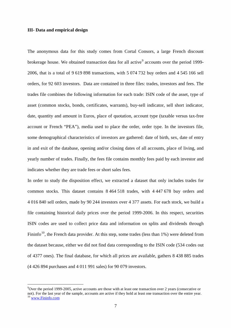
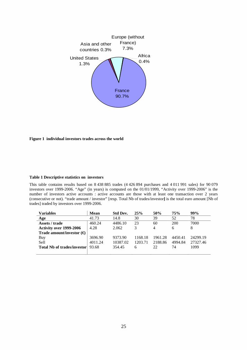
The second point relies on the international diversification of investors’ trades. Only 9,3% of
trades deal with non-French shares. it is not a surprising result because of the well-
documented home-bias (Huberman, 2001). Figure 1 provides precisely the distribution of
transactions across regions on our dataset. At the individual level, 54% of investors realize at
least one trade on these foreign assets and we call them “international traders”. Third, French
individual investors have a very easy access to short sales and 1095 investors realize all trades
using SRD orders; we call them “SRD investors” 11
The typical investor is a male (86,42%) and is 42 years old on average. Table 1 provides
descriptive statistics on trading behavior of investors. The average number of assets per trade
is nearly
.
Figure 1 about here
12
11Note that SRD (“Système à Règlement Différé”) is a French market specificity which allows investors to leverage and short sell. 12 This relatively high number of stocks per trade is mainly due to some huge trades on penny stocks.
460. During the period 1999-2006, investors realized more than 90 trades
amounting to an average of more than 3 800€ per trade (3 696€ for buy and 4 011€ for sell).
As the median trade size, number and amount are respectively 60 assets, 22 trades and

9
roughly 2000 €, we conclude that there is a considerable heterogeneity in the trading behavior
of investors. On average, investors are active half of the time (4 years over the 8).
Table 1 about here
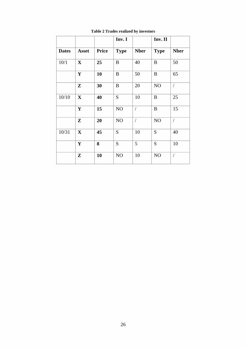
In this paper, we use the methodology given in Odean (1998) to compute the disposition
effect and the following example provides an explicit example. Suppose that two investors (I
and II) are active and that 3 stocks (X, Y, Z) are quoted on the financial market. Table 2
summarizes all investor’s trades on the whole period of study (one month for this example).
This table contains the dates (first column) when at least one of the two investors takes a
position (Buy or Sell). “Asset” and “Price” indicate respectively the number of assets and the
average price of the asset during the day. Columns “type” give the investor trade indicator:
purchase (B for Buy), sale (S for sell) or nothing (NO). “Nber” indicates the trade volume.
Table 2 about here
Each day an investor sells securities, we determine whether the security is sold for a gain or a
loss by comparing its selling price to its average purchase price. When the position changes
and stocks are bought, the average purchase price is then adjusted.
Therefore, each sale is counted as a realized gain (RG) or a realized loss (RL). Each stock in
the portfolio at the beginning of each day that is not sold during that day is considered to be
an unrealized (paper) gain or loss. Paper gains or losses are defined by comparing the high
and low daily price of the stock to its average purchase price. If these daily prices are above
their average purchase price, the trade is counted as a paper loss (PL); in the opposite case, it
is counted as a paper gain (PG); otherwise, neither a paper gain nor a loss is accounted for.

10
All gains and losses are calculated after adjusting for splits. Following Odean, we choose the
reference price to be the average purchase price.
To illustrate this methodology, in the example of table 2, on October the 10th, prices of X and
Y are higher than their average purchase prices (contrary to the price of Z) and the first
investor chooses to sell 10 stocks X and to keep his position on Y and Z.
Then, on this date and for this investor, we compute 1 realized gain (stocks X sold), 0 realized
loss, 1 paper gain (stocks Y) and 1 paper loss (stocks Z). Table 3 summarizes for the two
investors, the values of RG, RL, PG, PL, for all selling days.
Table 3 about here
It is important to notice that the four estimates, RG, RL, PG and PL could obviously not be
computed for portfolios containing only purchases or sales, portfolios with only one trade or
only one asset traded and for sales for which no previous purchase was identified. In this
article, the final number of trades for which the preceding methodology can be applied is
8 230 826.
The last step of the methodology consists of using these key values (RG, RL, PG and PL) to
compute the proportion of realized gains (PGR) and the proportion of realized losses (PLR)
according to the following rules:
RG
RG PG
RL
RL PL
NPGRN N
NPLRN N
DE PGR PLR
=+
=+
= −
where , , , denote the number of realized gains, the number of potential gains (paper gains),
the number of realized losses and the number of potential losses (paper losses).
11
In this paper, the measure of the disposition effect is defined as the difference DE = PGR -
PLR. When this difference takes a positive value, it indicates that investors are more prone to
realize gains than losses. In our example, the last row of Table 3 (TOTAL) gives RGN = 3,
RLN = 2, PGN = 1 and PLN = 3. Finally, PGR = 0.75, PLR = 0.4 and DE = 0.35.
It is important to notice that these values are computed across investors assuming that each
sale for a gain (or a loss) and paper gain (or paper loss) on the day of the sale are separate
independent observations. In this context, we test the following hypothesis:
PLRLPGRG NNPLRPLR
NNPGRPGR
PLRPGRZ
+−
++−
−=
)1()1(
: Proportion of Gains Realized ≤ Proportion of Losses Realized
The Z-statistic (distributed normally) is applied to test this hypothesis where:
Note that assuming the independence at an account level (instead of at a transaction level)
PGR, PLR and DE could be measured for each investor (instead of at an aggregate level) 13.
The global disposition effect is then defined as the average account disposition effect. In our
example, Total I and Total II give the values of , , , that are used to compute the
disposition effect at an individual level. After basic calculations the value of the average
disposition effect is 0.415 (0.33 for the first investor and 0.5 for the second)14
13 For a discussion on the limits of these measures, see for example Feng and Seasholes (2005) 14 Contrary to our simple illustration, in order to control for independence at an account level, the sale of a stock is counted only if no sale has been previously counted for that stock in any account within a week before or after the sale date (Odean, 1998).
.
This simple illustration shows that the two measures of ED give obviously different results
and even if at an aggregated level investors seem to suffer from the disposition effect, the
disparity between investors may be very important.
12
In the following sections, the disposition effect is first studied globally based on the
assumption on independence at the transaction level. Then we study the presence of the
disposition effect among sub-groups of traders. In the last section, we measure the impact of
the tax account type on the behavior of investors and then use an individual measure of the
disposition effect.
IV – General results and discussion
IV – 1 Disposition effect and sophistication
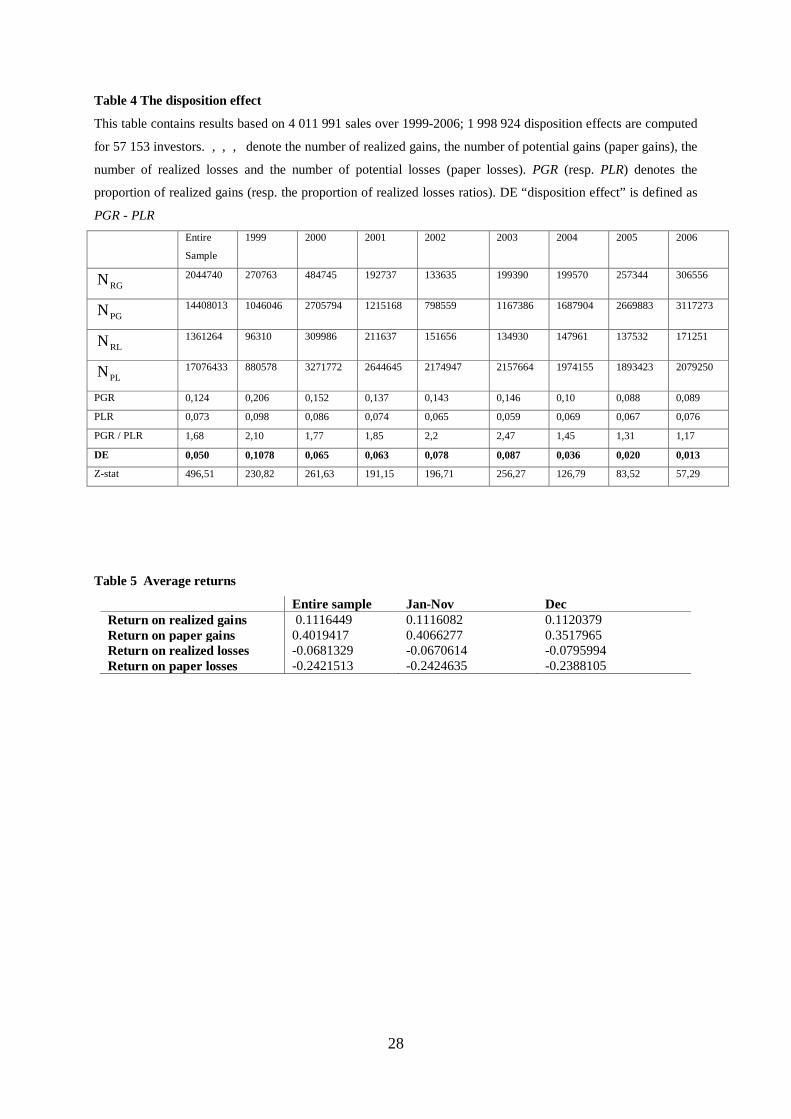
In this section, we present the results at the aggregate level. Based on 4 011 991 sales, we
compute a total of 1 998 924 disposition effects for 57 153 investors15. For sake of simplicity,
investors for whom a disposition effect is computed are called “investors” in the rest of the
paper. We study the aggregate disposition effect (see tables 2 and 3 for an example) by
considering that each sale that results in a realized or paper gain/loss constitutes an
independent observation. An alternative way to study the disposition effect is to consider that
realized/paper gains and losses are independent, not at the transaction level, but at the account
or investor level. In Table 4, we provide the average values of PGR, PLR and DE over
1 998 924 independent observations16
.
Table 4 about here
15 Note that if many operations are recorded on the same day, a unique disposition effect is computed. 16 We also use this methodology over our dataset (see figure 4 in the appendix) and find that approximately 20 % of the investors do not exhibit any DE or exhibit the opposite behaviour (DE < 0). This result confirms the ones obtained by Dhar and Zhu (2006) on US individual investors.

13
On the entire sample, the null hypothesis (PGR ≤ PLR ) is rejected with a high degree of
statistical significance. Investors are prone to the disposition effect over our sample period.
Note that the results differ across years. For example, in 1999 the aggregate disposition effect
is the highest (0.1078) whereas 2006 exhibits the lowest DE value (0.013).
However, looking at the evolution of the average DE and of the ratio PGR/PLR, we cannot
highlight any distinct monotonic trend over time. For example, PGR/PLR values gradually
increase from 2000 to 2002, peaking in 2003 and falling off as from 2004. The ratio PGR to
PLR is the rate at which the individual investors prefer to sell winning stocks rather than
losing ones. On the average, a stock that is up in value is more than 60% (1.68) more likely to
be sold that a stock that is down. These results are quite in line with those generally obtained
in the literature: Odean (1998) and Weber and Welfens (2006) compute a ratio of 1.5 while
Brown et al. (2006) and Chen et al. (2007) get 1.6.
For a better understanding of the behavior of the investors, Table 5 (column 1) gives the
average returns since the day of purchase for realized and paper gains and losses for the entire
sample. Returns on paper gains are fourfold greater than those on realized gains. The same
type of conclusion is obtained for losses (last two rows of Table 5). As noted by Odean
(1998), these results seem to confirm that investors are more likely to realize smaller, rather
than larger, gains and losses
Table 5 about here
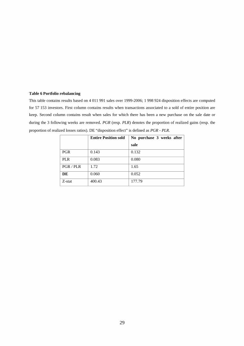
We also test whether the disposition effect observed in our sample can be explained by the
desire of individuals to rebalance their portfolios (Table 6, column 1) or to restore
diversification (Table 6, column 2). For the first test, we eliminate any sale for which the
entire position in a stock has not been cleared (53 502 investors sold their entire position in
14
the database). To eliminate any transaction resulting from a desire to restore diversification,
we also remove sales for which there has been a new purchase on the sale date or during the 3
following weeks (21 days). 48 523 traders are concerned. Our results confirm previous results
by demonstrating that traders still prefer to sell winners. The magnitude of the disposition
effect is not reduced on this restricted sample.
Table 6 about here
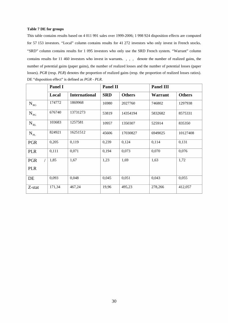
In order to investigate the influence of traders’ sophistication on the disposition effect, we
build different groups of traders and check whether they exhibit any disposition effect. Three
proxies for investors skills are retained; the geographical diversification of trades (presence of
trades outside France), the use of the French SRD (“Système à Règlement Différé”) and the
investment in warrants. Briefly speaking, although individual investors are not usually
supposed to be sophisticated ones, we assume that among them, those who internationally
diversify portfolios (or are subject to a less important home bias), trade with SRD or trade
warrants are at least more familiar with financial markets.
According to the ISIN of stocks, we divide investors in two categories: 40 430 among them
only invest in French stocks, and we call them “local traders”, the others are “international
traders”. Results in Table 7 panel I indicate that both groups are prone to the bias. More
precisely, the disposition effect for “local traders” is 0.093 which is twofold the value of the
disposition effect of “international traders”.
Table 7 about here
15
Note that PGR and PLR measures are dependent on the portfolio size; we could obtain a
lower disposition bias for an individual trading frequently but realizing the same number of
winners/ losers. We should however point out that Dhar and Zhu (2006) compare measures of
DE over sub groups. They justify such comparisons by the relative homogeneity of portfolios
size among groups. Therefore, we computed the number of stocks held by individuals in each
of our sub-groups: local traders have on average 14 securities while international investors
hold 33 stocks. Given the difference in portfolio sizes, we do not compare our measures of
DE17. The same argument applies to the other two proxies for sophistication (warrants and
SRD use) although these proxies are not directly linked to trading behavior18
Results in Table 7, panels II (SRD) and III (warrants), indicate that the 4 groups are prone to
the bias and that the disposition effect appears to be slightly lower for sophisticated traders
(DE is 0.045 for SRD investors and 0.043 for warrant investors against 0.051 and 0.055 for
the respective non sophisticated investors). Though more investigation is clearly needed,
sophistication seems to attenuate the DE which order of magnitude is 0.04 for all
sophisticated investors (0.048 for international traders)
during the
sample period as they rely on the presence of specific trades in each investor account. A
“SRD” investor always chooses to use the leverage and short selling facility; there are 1 095
such investors. A “warrant” investor trades warrants at least once during the sample period;
there are 11 460 such investors.
19
.
17 For a discussion of DE determinants, see for example Feng and Seasholes (2005). 18 Note that “warrants” trades are excluded from our dataset. 19 We also use the trading activity (based on the number of annual transactions) as another proxy and find DE=0.04 for frequent investors. We do not report these results because we think trading activity constitutes a proxy for experience that does not always hint to sophistication.

16
IV – 2 Disposition effect and taxes
In this subsection, we first analyze the existence of end-of-the-year effect on the disposition
effect (tax impact). Secondly, with respect to French specificities, we also investigate whether
account types and tax regime shifts influence investment behavior.
In order to investigate whether individual investors pay attention to tax considerations at the
end of the fiscal year, we also compute PGR, PLR and DE over the two intra year periods,
January-November and December. Drawing on the work of Constantinides (1984), we expect
investors to gradually increase their tax-loss selling from January to December. Table 8
provides the results.
Table 8 about here
We test the differences in proportions over the two sub-periods. Formally, for two
independent samples (1) and (2), we test the following hypothesis:
and
: Proportion of Gains Realized in (2) = Proportion of Gains Realized in (1)
’
: Proportion of Losses Realized in (2) = Proportion of Losses Realized in (1)
The following statistic (normally distributed) is applied to test
( ) ( )( ) ( )
( ) ( )
0
2 2 1 1
2 2 1 1
2 2 1 1
2 1
2 1
1 1ˆ ˆ(1 )
ˆ
H
RG PG RG PG
RG PG RG PG
RG PG RG PG
PGR PGRT
N N N N
N N PGR N N PGRwith
N N N N
π π
π
−=
− + + +
+ + +=
+ + +
where:

17
jRGN and jPGN denote the number of realized gains and of potential gains (paper gains) in
sample j.
In previous studies, DE is generally negative and the PGR/PLR ratio is lower than 1 in the last
month of the fiscal year (December in US market for Odean (1998) and June for Brown et al.
(2006) in Australia, for example).
In table 8, the disposition effect seems to be lower in December when compared with the
average value of January-November but it is still positive. Tests of differences in proportions
indicate that the following results are significant: -Nov > and > -Nov
Moreover, looking in table 8 at PGR/PLR indicates that on average, traders realize fewer
gains and more losses in December: the ratio of PGR over PLR being 1.57 in December
against 1.68 for the entire year. However, the fiscal impact in France appears to be moderate
relative to the one observed in other countries as PGR/PLR remains higher than one in
December.
. These tests show that
the lower DE in December is due to an average lower PGR and a higher PLR in December.
This result differs from Odean’s conclusion of a lower DE in December which was due to
both significantly higher PLR and PGR in December.
The results in Table 5 (column 2 and 3) also help to confirm the presence of a moderate fiscal
impact at the end of the year. Returns on realized paper losses are –0,079 in December against
-0,068 for the entire year. These results are clearly different from Odean ones who obtain a
greater difference between these two values (-0,366 in December against -0,228).
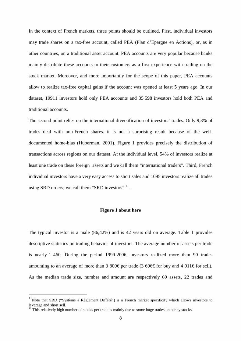
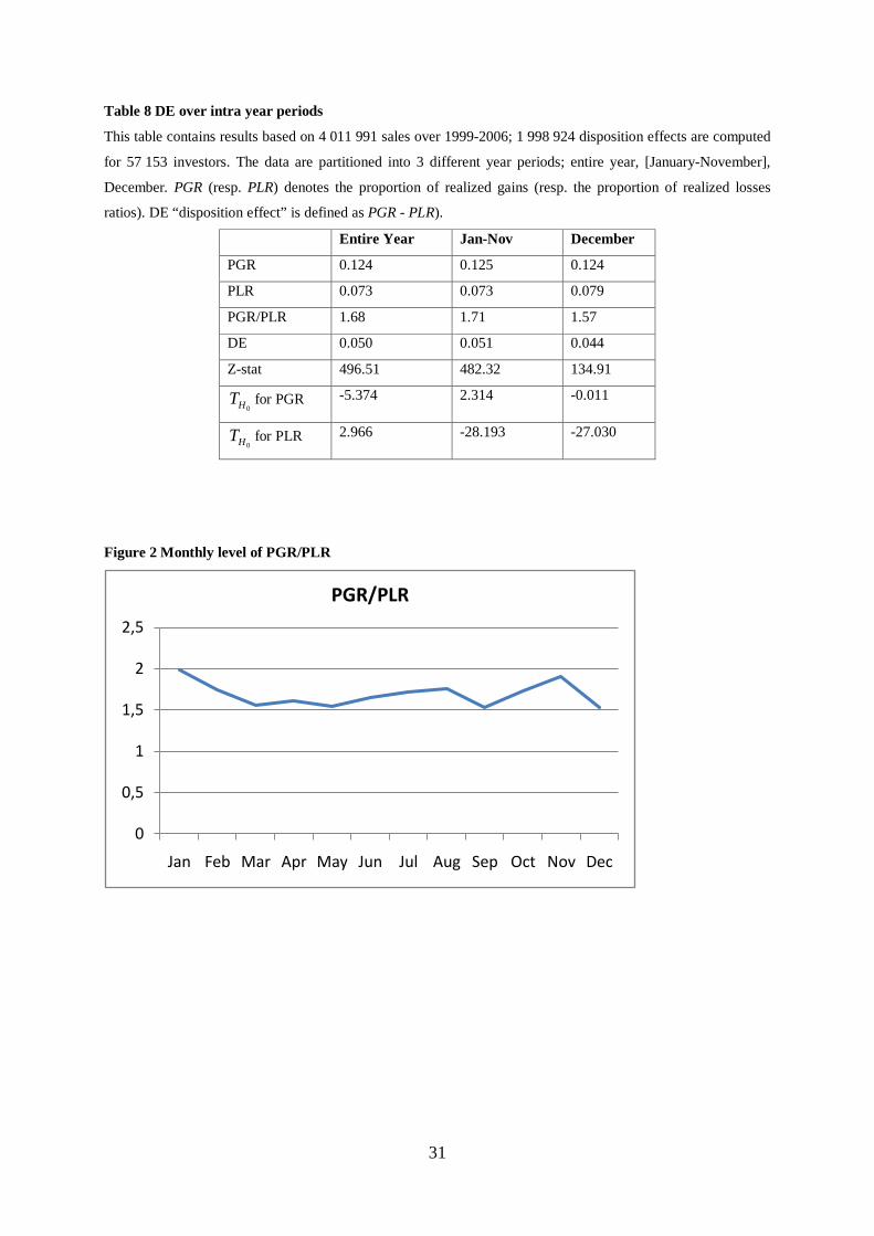
Finally, Figure 2 plots the average ratio of PGR/PLR on a monthly basis. We notice that
contrary to Constantinides’ (1984) arguments, investors do not gradually decrease the rate at
which they sell winning stocks compared to losing ones during the year.
18
Figure 2 about here
In the French case, the fiscal impact on the selling behavior of investors could be tested in an
original way due to the tax regime of some accounts (PEA accounts). Actually, capital gains
are tax-free for all trades occurring 5 years after the opening date of the account. To be more
precise, it is important to understand that fiscal exoneration occurs even if stocks were not
kept for more than 5 consecutive years. The only legal restriction imposed before 5 years is
that investors can’t withdraw cash resulting from sales. For example, a capital gain on a
round-trip trade made five years after the inception date of the account is tax-free.
Therefore, as investors may choose to trade on both accounts, we expect to measure the
impact of tax on selling behavior by highlighting different behaviors on PEA accounts and
traditional accounts. To serve our purpose, we focus our analysis on investors trading both on
PEA and traditional accounts20
Table 9 gives the results obtained for the 2 116 investors (Group I) at an aggregate level.
Global results indicate that the disposition effect is clearly positive and significant before and
. In this context, for any holder of a PEA account, 5 years
represents a focal point (beginning of the tax-free period). If investors are sensitive to taxes,
we expect buy and sell decisions to be affected by the tax shift on the PEA account after 5
years. To control our results, we study the same behavioral patterns for the same investors on
traditional accounts.
We identify traders holding more than five years old PEA and traditional accounts (2 116
investors that we call “GROUP I”) and classify trades made on these accounts according to
their execution date. In other words, we distinguish trades that were realized before and those
realized after the accounts reached the focal point of five years. This ensures a good
comparative basis for any analysis of possible different behaviors.
20 On the entire sample, there are 35 598 such traders. Note that there are 46 094 holders of only traditional accounts and 10 911 holders of only PEA in the database.
19
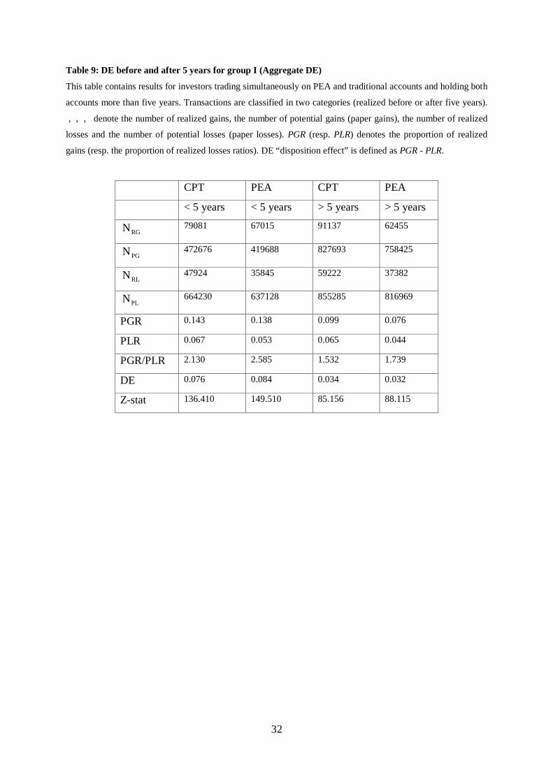
after five years on both accounts. Accurately, on traditional accounts, the DE before five years
is 0.076 (column 1) and 0.034 for trades made after five years (column 3). For PEA accounts
values are 0.084 (column 2) and 0.032 (column 4). At an aggregate level we observe that DE
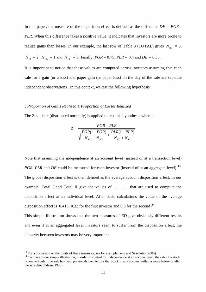
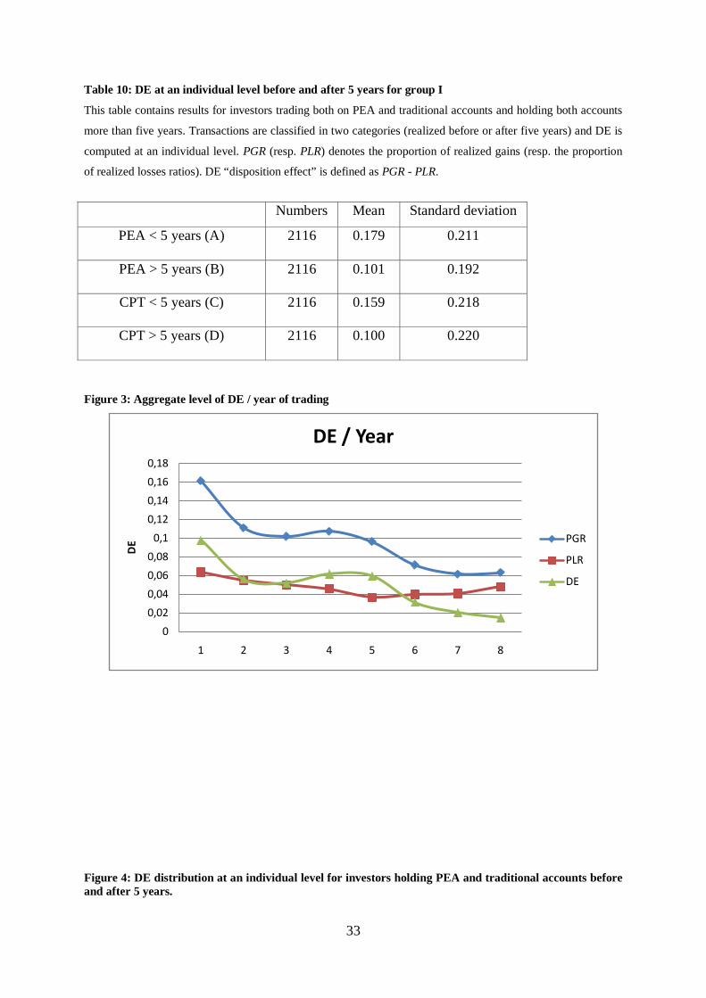
decreases between the two sub-periods whatever the account type21. Figures 3 confirms this
result and gives a more precise illustration of the evolution of the aggregate DE with respect
to experience (years of trading) for the 2110 investors. For example, at the end of the second
year of trading DE is 0,056 and at the end of the seventh year of trading the value is about
0,02. This curve could be seen as an “experience curve” and the decreasing trend could be
linked to the role played by the number of years of trading ; the impact of this variable was
demonstrated in previous studies (Dhar and Zhu, 2006, Shu et al. 2005, Brown et al., 2006 for
example) 22.
Table 9 about here
To investigate more accurately the hypothetic tax impact on selling behaviors, we compute
the disposition effect at an individual level for the 2 116 investors belonging to Group I before
and after the
21 Note that results for the 1665 investors trading only on PEA accounts and keeping this account for more than five years (Group II) and for the 5114 investors trading only on traditional accounts and keeping this account for more than five years (Group III) confirm this point (see table 12 in the appendix). 22 Note that the decrease of DE is essentially imparted to the decrease of PGR, investors seems to correct this bias in an asymmetrical way.
birthday of both accounts.
The results for these investors are given in Table 10. Accurately, on traditional accounts, the
DE before five years is 0.159 and 0.1 for trades made after five years. For PEA accounts
values are 0.179 and 0.101. This table confirms the decrease of the individual average
disposition effect after 5 years on the two account types and again highlights the results
obtained at the aggregate level.
20
However, to control for any global compensation between investors, we conduct a Wilcoxon
signed rank test of individual DE differences.
This test uses both the information on the direction and the relative magnitude of the
differences within pairs of an identical trader average DE. For two distributions X and Y, the
null hypothesis of the test is the following:
: X and Y are samples from populations with same continuous distributions.
Table 10 about here
Figure 3 about here
Table 11 gives the results of the tests for the differences in distributions between types of
accounts and detention duration. We denote (A) [resp. B] the distribution of the individual DE
for trades over PEA before 5 years [resp. after 5 years] and (C) [resp. D] is the distribution of
DE for trades on traditional account before 5 years [resp. after 5 years]. V is the number of
ranks of positive differences. Note that as N=2116 is a large sample size, the number of the
ranks of positive differences, V, is approximately normal.
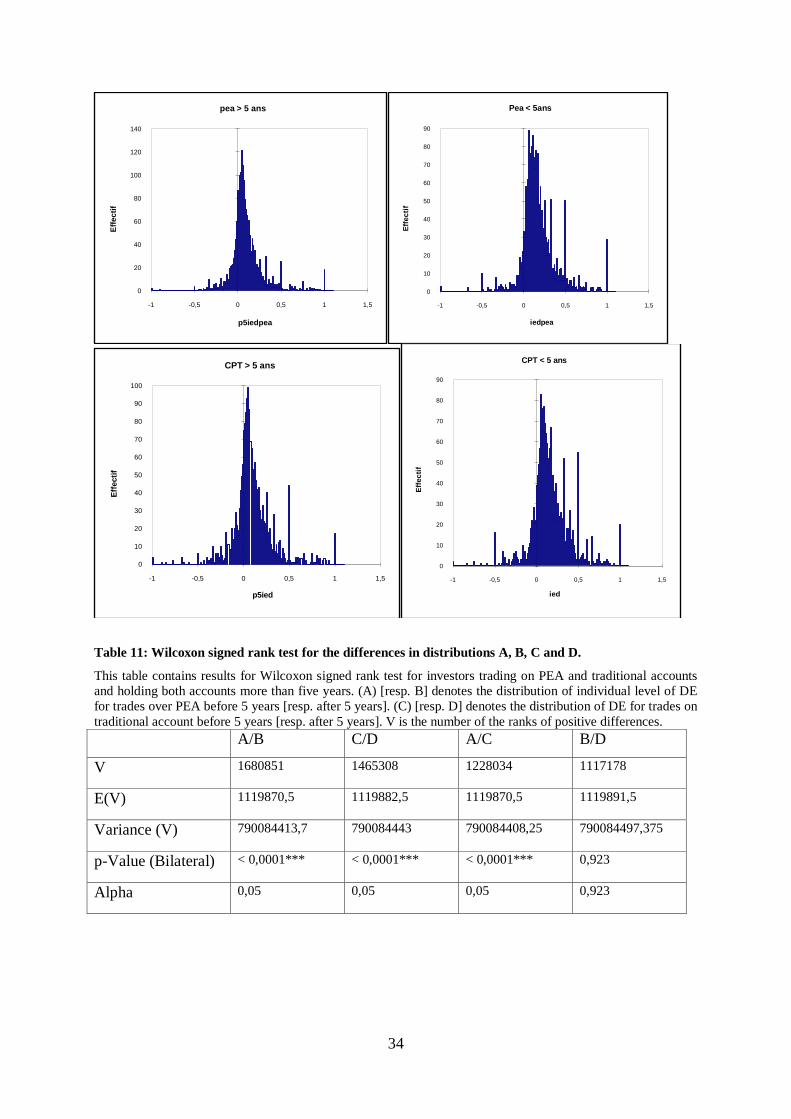
The two first columns (A/B and C/D) show that individual distributions before and after are
significantly different given account types. The behavior of investors seems to be clearly
different as experience increases; this confirms the importance of learning already highlighted
at an aggregate level (see figure 3). The test on B/D distributions allows us to reject the tax
argument for the PEA account. Actually, in the period of different taxation between both
accounts, no difference of trading behavior in any direction could be detected at an individual
level.

21
Table 11 about here
V Conclusion
We provide first and original results on the behavior of investors in the French context. On a
large and proprietary anonymous database provided by Cortal Consors, a French broker, we
find strong evidence that the disposition effect is observed for different categories of investors
and for all time periods. Moreover this mistaken behavior does not seem to be motivated by a
desire to rebalance portfolios.
As we expect some particular traders to be more sophisticated than others, based on original
proxies (international diversification, SRD use, for example) we demonstrate that
sophistication does not eliminate the existence of a disposition bias.
In this paper we conduct two tests of the impact of taxes on the selling behavior. First, at an
aggregate level we find that investors are less prone to the disposition effect in December than
during the rest of the year (due to a higher PGR and a lower PLR). Moreover, investors seem
to realize losses of slightly stronger magnitude in December. However, unlike previous
studies, DE is still positive (and PGR/PLR is higher than 1) in the last month of the fiscal year
(Odean (1998), Brown et al. (2006), for example). Secondly, an analysis of a French
specificity, i.e. the existence of tax free accounts (PEA more than 5 years old) allows us to
demonstrate that accounts tax regimes have no impact on selling behavior.
Finally, this work could be extended at least in order to highlight characteristics of individual
investors explaining the level of the disposition effect and its dynamics.
22
References Barber, B. M., Y. T. Lee, Y. J. Liu and T. Odean. 2007. Is the Aggregate Investor Reluctant to Realize
Losses? Evidence from Taiwan. European Financial Management, 13(3), 423–447.
Barberis, N. and W. Xiong. 2006. What Drives the Disposition Effect? An Analysis of a Longstanding
Preference Based Explanation. Forthcoming Journal of Finance.
Barberis, N. and W. Xiong. 2008. Realization Utility. Working Paper, Yale University.
Brockner, J. 1992. The Escalation of Commitment to a Failing Course of Action: Toward Theoretical
Progress. The Academy of Management Review, 17, 39-61.
Brown, P., N. Chappel, R. da Silva Rosa, and T. Walter. 2006. The reach of the disposition effect:
Large sample evidence across investor classes, International Review of Finance, 6(1-2), 43-78.
Chen, G.M, K. A. Kim, J. R. Nofsinger and O. M. Rui . 2004. Behavior and performance of emerging
market investors: Evidence from China. Working paper.
Chui, P. 2001. An Experimental Study of the Disposition Effect: Evidence From Macau. The Journal
of Psychology and Financial Markets, 2(4), 216-222.
Constantinides, G. 1984. Optimal Stock Trading with Personal Taxes: Implications for Prices and the
Abnormal January Returns. Journal of Financial Economics, 13, 65-89.
Coval, J. D. and T. Shumway 2005. Do Behavioral Biases Affect Prices? Journal of Finance, 60(1), 1-
34.
Dhar, R. and N. Zhu. 2006. Up Close and Personal: Investor Sophistication and the Disposition Effect.
Management Science, 52(5) 726-740.
Feng, L. and M. Seasholes 2005. Do Investor Sophistication and Trading Experience Eliminate
Behavioral Biases in Financial Markets ? Review of Finance, 9, 305-351.
Ferris, S., R. Haugen and A. Makhija. 1988. Predicting Contemporary Volume with Historic Volume
at Differential Price Levels: Evidence Supporting the Disposition Effect. Journal of Finance, 43(3),
677-697.
Frino, A., D. Johnstone and H. Zheng. 2005. The Propensity for Local Traders in Futures Markets to
Ride Losses: Evidence of Irrational or Rational Behavior? Journal of Banking and Finance, 28 ,353-
372.
Genesove, D. and C. Mayer. 2001. Loss Aversion and Seller Behavior: Evidence from the Housing
Market. The Quarterly Journal of Economic, 116(4), 1233-1260.
Grinblatt, M., et M. Keloharju. 2001. What Makes Investors Trade? Journal of Finance, 56, 589-616.
Heath, C., S. Huddart and M. Lang. 1999. Psychological Factors and Stock Option Exercise. The
Quarterly Journal of Economics, 114 (2), 601-627.
Hens, T. and M.Vlcek. 2005. Does Prospect Theory Explain the Disposition Effect? NHH Dept. of
Finance & Management Science, Discussion Paper No. 18.
23
Huberman, G. 2001. Familiarity breeds investment. Review of Financial Studies, 14, 659-680.
Kahneman, D. and A. Tversky. 1979. Prospect Theory: an Analysis of Decision under Risk.
Econometrica, 47, 263-291.
Kyle, S.A., H. Ou-Yang and W. Xiong. 2006. Prospect Theory and Liquidation Decisions. Journal of
Economic Theory, 129, 273-288.
Lakonishok, J. and S. Smidt. 1986. Volume for Winners and Losers: Taxation and Other Motives for
Stock Trading. Journal of Finance, 41(4), 951-974.
Locke, P. and S. Mann. 2003. Professional Trader Discipline and Trade Disposition. Working Paper,
George Washington University.
Muermann, A. And J.M. Volkman. 2006. Regret, Pride and the Disposition Effect. Working Paper,
Wharton School.
O’Curry Fogel, S. and T. Berry. 2006. The disposition effect and individual investor decisions: the
roles of regret and counterfactual alternatives. Journal of Behavioral Finance, 7(2), 107-116.
Odean, T. 1998. Are Investors Reluctant to Realize Their Losses? Journal of Finance, 53(5), 1775-
1798.
Rubaltelli, E., S. Rubichi, L. Savadori, M. Tedeshi and R. Ferretti. 2005. Numerical Information
Format and Investment Decisions: Implications for the Disposition Effect and the Status Quo Bias.
The Journal of Behavioral Finance, 6(1), 19-26.
Shapira, Z. and I. Venezia. 2001. Patterns of Behavior of Professionally Managed and Independent
Investors. Journal of Banking and Finance, 25(8), 1573-1587.
Shefrin, H. and M. Statman. 1985. The Disposition to Sell Winners Too Early and Ride Losers Too
Long: Theory and Evidence, Journal of Finance, 40, 777-790.
Shu, P.G., Y.H. Yeh, S.B. Chiu and H.C. Chen. 2005. Are Taiwanese individual investors reluctant to
realize their losses? Pacific Basin Finance Journal, 25(2), 201-223.
Staw, B.M. 1979. Knee-deep in the Big Muddy: a Study of Escalating Commitment to a Chosen
Course of Action. Organizational Behavior and Human Performance, 16, 27-44.
Thaler, R. H. and E. J. Johnson. 1990. Gambling with the House Money and Trying to Break Even;
the Effects of Prior Outcomes on Risky Choice. Management Science, 36(6), 643-660.
Tversky, A. and D. Kahneman. 1992. Advances in prospect theory: cumulative representation of
uncertainty. Journal of Risk and Uncertainty, 5, 232– 297.
Weber, E. and Hsee, C. (1998). Cross-cultural differences in risk perception but cross-cultural
similarities in attitudes towards risk. Management Science, 44, 1205-1217.
Weber, M. and C. F. Camerer. 1998. The Disposition Effect in Securities Trading: An Experimental
Analysis. Journal of Economic Behaviour and Organization, 33(2), 167-184.
Weber, M. and H. Zuchel. 2005. How Do Prior Outcomes Affect Risk Attitude? Comparing
Escalation of Commitment and the House Money Effect. Decision Analysis, 2(1), 30-43.

24
Weber, M. and F. Welfens. 2006. An individual Level Analysis of the disposition Effect: Empirical
and Experimental Evidence. Working Paper. University of Mannheim.
Zuchel, H. 2001. Why Drives the Disposition Effect? Working Paper, University of Mannheim.
25
Figure 1 individual investors trades across the world
Table 1 Descriptive statistics on investors
This table contains results based on 8 438 885 trades (4 426 894 purchases and 4 011 991 sales) for 90 079 investors over 1999-2006. “Age” (in years) is computed on the 01/01/1999, “Activity over 1999-2006” is the number of investors active accounts : active accounts are those with at least one transaction over 2 years (consecutive or not). “trade amount / investor” [resp. Total Nb of trades/investor] is the total euro amount [Nb of trades] traded by investors over 1999-2006.
Variables Mean Std Dev. 25% 50% 75% 99% Age 41.73 14.8 30 39 52 78 Assets / trade 460.24 4486.10 23 60 200 7000 Activity over 1999-2006 4.28 2.062 3 4 6 8 Trade amount/investor (€) Buy 3696.90 9373.90 1168.18 1961.28 4450.41 24299.19 Sell 4011.24 10387.02 1203.71 2188.86 4994.84 27327.46 Total Nb of trades/investor 93.68 354.45 6 22 74 1099
France 90.7%
Africa0.4%
Europe (without France)7.3%
United States1.3%
Asia and other countries 0.3%
26
Table 2 Trades realized by investors
Inv. I Inv. II
Dates Asset Price Type Nber Type Nber
10/1 X 25 B 40 B 50
Y 10 B 50 B 65
Z 30 B 20 NO /
10/10 X 40 S 10 B 25
Y 15 NO / B 15
Z 20 NO / NO /
10/31 X 45 S 10 S 40
Y 8 S 5 S 10
Z 10 NO 10 NO /

27
Table 3 Key values for the two investors
RG RL PG PL
INV I
10/10 1 0 1 1
10/31 1 1 0 1
Total I 2 1 1 2
INV II
10/31 1 1 0 1
Total II 1 1 0 1
TOTAL (I +II) 3 2 1 3
28
Table 4 The disposition effect This table contains results based on 4 011 991 sales over 1999-2006; 1 998 924 disposition effects are computed
for 57 153 investors. , , ,
denote the number of realized gains, the number of potential gains (paper gains), the
number of realized losses and the number of potential losses (paper losses). PGR (resp. PLR) denotes the
proportion of realized gains (resp. the proportion of realized losses ratios). DE “disposition effect” is defined as
PGR - PLR Entire
Sample
1999 2000 2001 2002 2003 2004 2005 2006
RGN 2044740 270763 484745 192737 133635 199390 199570 257344 306556
PGN 14408013 1046046 2705794 1215168 798559 1167386 1687904 2669883 3117273
RLN 1361264 96310 309986 211637 151656 134930 147961 137532 171251
PLN 17076433 880578 3271772 2644645 2174947 2157664 1974155 1893423 2079250
PGR 0,124 0,206 0,152 0,137 0,143 0,146 0,10 0,088 0,089
PLR 0,073 0,098 0,086 0,074 0,065 0,059 0,069 0,067 0,076
PGR / PLR 1,68 2,10 1,77 1,85 2,2 2,47 1,45 1,31 1,17
DE 0,050 0,1078 0,065 0,063 0,078 0,087 0,036 0,020 0,013
Z-stat 496,51 230,82 261,63 191,15 196,71 256,27 126,79 83,52 57,29
Table 5 Average returns
Entire sample Jan-Nov Dec Return on realized gains 0.1116449 0.1116082 0.1120379 Return on paper gains 0.4019417 0.4066277 0.3517965 Return on realized losses -0.0681329 -0.0670614 -0.0795994 Return on paper losses -0.2421513 -0.2424635 -0.2388105
29
Table 6 Portfolio rebalancing
This table contains results based on 4 011 991 sales over 1999-2006; 1 998 924 disposition effects are computed
for 57 153 investors. First column contains results when transactions associated to a sold of entire position are
keep. Second column contains result when sales for which there has been a new purchase on the sale date or
during the 3 following weeks are removed. PGR (resp. PLR) denotes the proportion of realized gains (resp. the
proportion of realized losses ratios). DE “disposition effect” is defined as PGR - PLR.
Entire Position sold No purchase 3 weeks after
sale
PGR 0.143 0.132
PLR 0.083 0.080
PGR / PLR 1.72 1.65
DE 0.060 0.052
Z-stat 400.43 177.79
30
Table 7 DE for groups
This table contains results based on 4 011 991 sales over 1999-2006; 1 998 924 disposition effects are computed
for 57 153 investors. “Local” column contains results for 41 272 investors who only invest in French stocks.
“SRD” column contains results for 1 095 investors who only use the SRD French system. “Warrant” column
contains results for 11 460 investors who invest in warrants. , , ,
denote the number of realized gains, the
number of potential gains (paper gains), the number of realized losses and the number of potential losses (paper
losses). PGR (resp. PLR) denotes the proportion of realized gains (resp. the proportion of realized losses ratios).
DE “disposition effect” is defined as PGR - PLR.
Panel I Panel II Panel III
Local International SRD Others Warrant Others
RGN 174772 1869968 16980
2027760
746802
1297938
PGN 676740 13731273 53819
14354194
5832682
8575331
RLN 103683 1257581 10957
1350307
525914
835350
PLN 824921 16251512 45606
17030827
6949025
10127408
PGR 0,205 0,119 0,239
0,124
0,114
0,131
PLR 0,111 0,071 0,194
0,073
0,070
0,076
PGR /
PLR
1,85 1,67 1,23
1,69
1,63
1,72
DE 0,093 0,048 0,045
0,051
0,043
0,055
Z-stat 171,34 467,24 19,96
495,23
278,266
412,057
31
Table 8 DE over intra year periods
This table contains results based on 4 011 991 sales over 1999-2006; 1 998 924 disposition effects are computed
for 57 153 investors. The data are partitioned into 3 different year periods; entire year, [January-November],
December. PGR (resp. PLR) denotes the proportion of realized gains (resp. the proportion of realized losses
ratios). DE “disposition effect” is defined as PGR - PLR).
Entire Year Jan-Nov December
PGR 0.124 0.125 0.124
PLR 0.073 0.073 0.079
PGR/PLR 1.68 1.71 1.57
DE 0.050 0.051 0.044
Z-stat 496.51 482.32 134.91
0HT for PGR -5.374 2.314 -0.011
0HT for PLR 2.966 -28.193 -27.030
Figure 2 Monthly level of PGR/PLR
0
0,5
1
1,5
2
2,5
Jan Feb Mar Apr May Jun Jul Aug Sep Oct Nov Dec
PGR/PLR
32
Table 9: DE before and after 5 years for group I (Aggregate DE)
This table contains results for investors trading simultaneously on PEA and traditional accounts and holding both
accounts more than five years. Transactions are classified in two categories (realized before or after five years). , , ,
denote the number of realized gains, the number of potential gains (paper gains), the number of realized
losses and the number of potential losses (paper losses). PGR (resp. PLR) denotes the proportion of realized
gains (resp. the proportion of realized losses ratios). DE “disposition effect” is defined as PGR - PLR.
CPT PEA CPT PEA
< 5 years < 5 years > 5 years > 5 years
RGN 79081 67015 91137 62455
PGN 472676 419688 827693 758425
RLN 47924 35845 59222 37382
PLN 664230 637128 855285 816969
PGR 0.143 0.138 0.099 0.076
PLR 0.067 0.053 0.065 0.044
PGR/PLR 2.130 2.585 1.532 1.739
DE 0.076 0.084 0.034 0.032
Z-stat 136.410 149.510 85.156 88.115
33
Table 10: DE at an individual level before and after 5 years for group I
This table contains results for investors trading both on PEA and traditional accounts and holding both accounts
more than five years. Transactions are classified in two categories (realized before or after five years) and DE is
computed at an individual level. PGR (resp. PLR) denotes the proportion of realized gains (resp. the proportion
of realized losses ratios). DE “disposition effect” is defined as PGR - PLR.
Numbers Mean Standard deviation
PEA < 5 years (A) 2116 0.179 0.211
PEA > 5 years (B) 2116 0.101
0.192
CPT < 5 years (C) 2116 0.159
0.218
CPT > 5 years (D) 2116 0.100
0.220
Figure 3: Aggregate level of DE / year of trading
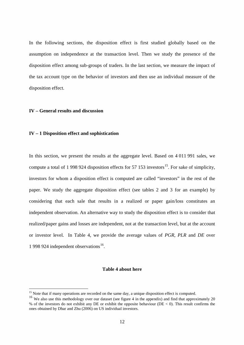
Figure 4: DE distribution at an individual level for investors holding PEA and traditional accounts before and after 5 years.
0
0,02
0,04
0,06
0,08
0,1
0,12
0,14
0,16
0,18
1 2 3 4 5 6 7 8
DE
DE / Year
PGR
PLR
DE
34
Table 11: Wilcoxon signed rank test for the differences in distributions A, B, C and D.
This table contains results for Wilcoxon signed rank test for investors trading on PEA and traditional accounts and holding both accounts more than five years. (A) [resp. B] denotes the distribution of individual level of DE for trades over PEA before 5 years [resp. after 5 years]. (C) [resp. D] denotes the distribution of DE for trades on traditional account before 5 years [resp. after 5 years]. V is the number of the ranks of positive differences. A/B C/D A/C B/D
V 1680851
1465308
1228034
1117178
E(V) 1119870,5
1119882,5
1119870,5
1119891,5
Variance (V) 790084413,7
790084443
790084408,25
790084497,375
p-Value (Bilateral) < 0,0001*** < 0,0001***
< 0,0001***
0,923
Alpha 0,05 0,05 0,05 0,923
0
20
40
60
80
100
120
140
-1 -0,5 0 0,5 1 1,5
Effe
ctif
p5iedpea
pea > 5 ans
0
10
20
30
40
50
60
70
80
90
-1 -0,5 0 0,5 1 1,5
Effe
ctif
iedpea
Pea < 5ans
0
10
20
30
40
50
60
70
80
90
100
-1 -0,5 0 0,5 1 1,5
Effe
ctif
p5ied
CPT > 5 ans
0
10
20
30
40
50
60
70
80
90
-1 -0,5 0 0,5 1 1,5
Effe
ctif
ied
CPT < 5 ans
35
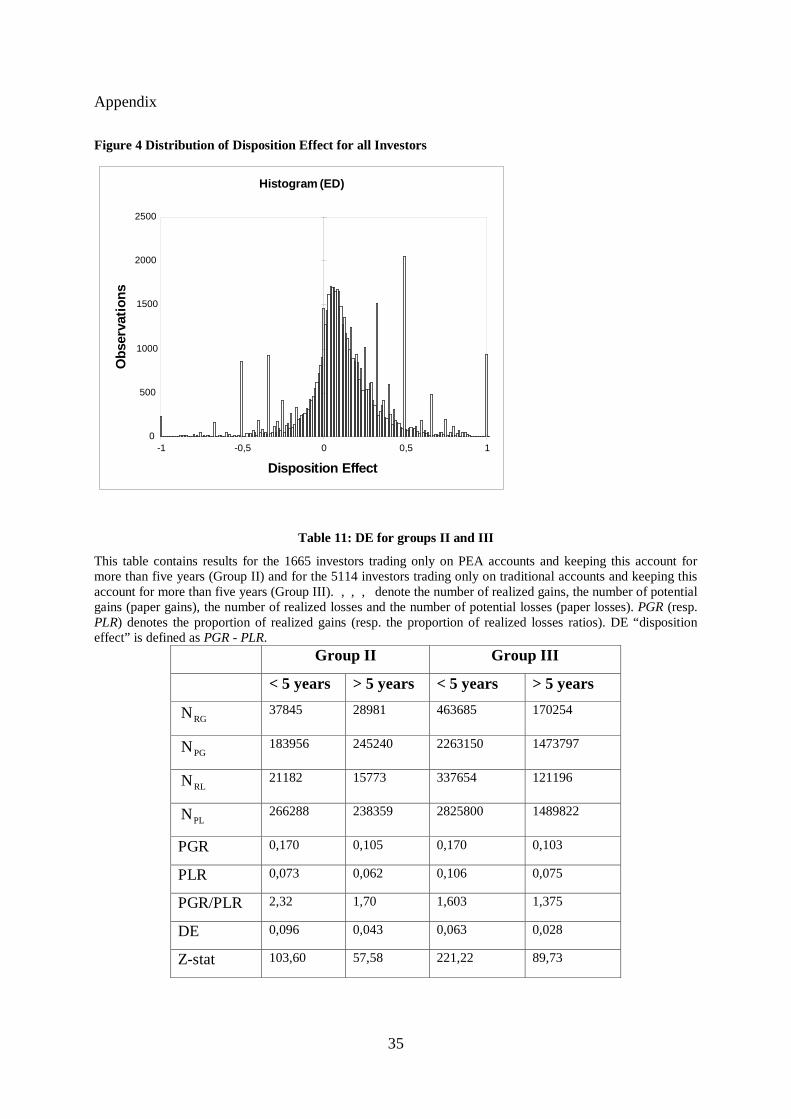
Appendix Figure 4 Distribution of Disposition Effect for all Investors
Table 11: DE for groups II and III
This table contains results for the 1665 investors trading only on PEA accounts and keeping this account for more than five years (Group II) and for the 5114 investors trading only on traditional accounts and keeping this account for more than five years (Group III). , , ,
denote the number of realized gains, the number of potential gains (paper gains), the number of realized losses and the number of potential losses (paper losses). PGR (resp. PLR) denotes the proportion of realized gains (resp. the proportion of realized losses ratios). DE “disposition effect” is defined as PGR - PLR.
Group II Group III
< 5 years > 5 years < 5 years > 5 years
RGN 37845 28981 463685 170254
PGN 183956 245240 2263150 1473797
RLN 21182 15773 337654 121196
PLN 266288 238359 2825800 1489822
PGR 0,170 0,105 0,170 0,103
PLR 0,073 0,062 0,106 0,075
PGR/PLR 2,32 1,70 1,603 1,375
DE 0,096 0,043 0,063 0,028
Z-stat 103,60 57,58 221,22 89,73
Histogram (ED)
0
500
1000
1500
2000
2500
-1 -0,5 0 0,5 1
Disposition Effect
Obs
erva
tions

PAPIERS
Laboratoire de Recherche en Gestion & Economie (LARGE)
______
D.R. n° 1 "Bertrand Oligopoly with decreasing returns to scale", J. Thépot, décembre 1993
D.R. n° 2 "Sur quelques méthodes d'estimation directe de la structure par terme des taux d'intérêt", P. Roger - N. Rossiensky, janvier 1994 D.R. n° 3 "Towards a Monopoly Theory in a Managerial Perspective",
J. Thépot, mai 1993 D.R. n° 4 "Bounded Rationality in Microeconomics", J. Thépot, mai 1993 D.R. n° 5 "Apprentissage Théorique et Expérience Professionnelle", J. Thépot, décembre 1993 D.R. n° 6 "Stratégic Consumers in a Duable-Goods Monopoly",
J. Thépot, avril 1994
D.R. n° 7 "Vendre ou louer ; un apport de la théorie des jeux", J. Thépot, avril 1994 D.R. n° 8 "Default Risk Insurance and Incomplete Markets", Ph. Artzner - FF. Delbaen, juin 1994 D.R. n° 9 "Les actions à réinvestissement optionnel du dividende",
C. Marie-Jeanne - P. Roger, janvier 1995 D.R. n° 10 "Forme optimale des contrats d'assurance en présence de coûts administratifs pour l'assureur", S. Spaeter, février 1995 D.R. n° 11 "Une procédure de codage numérique des articles",
J. Jeunet, février 1995 D.R. n° 12 Stabilité d'un diagnostic concurrentiel fondé sur une approche markovienne du comportement de rachat du consommateur",
N. Schall, octobre 1995 D.R. n° 13 "A direct proof of the coase conjecture", J. Thépot, octobre 1995 D.R. n° 14 "Invitation à la stratégie", J. Thépot, décembre 1995 D.R. n° 15 "Charity and economic efficiency", J. Thépot, mai 1996

D.R. n° 16 "Princing anomalies in financial markets and non linear pricing rules", P. Roger, mars 1996
D.R. n° 17 "Non linéarité des coûts de l'assureur, comportement de prudence de l'assuré et contrats optimaux", S. Spaeter, avril 1996 D.R. n° 18 "La valeur ajoutée d'un partage de risque et l'optimum de Pareto : une note", L. Eeckhoudt - P. Roger, juin 1996 D.R. n° 19 "Evaluation of Lot-Sizing Techniques : A robustess and Cost Effectiveness Analysis", J. Jeunet, mars 1996 D.R. n° 20 "Entry accommodation with idle capacity", J. Thépot, septembre 1996 D.R. n° 21 "Différences culturelles et satisfaction des vendeurs : Une comparaison internationale", E. Vauquois-Mathevet - J.Cl. Usunier, novembre 1996 D.R. n° 22 "Evaluation des obligations convertibles et options d'échange",
A. Schmitt - F. Home, décembre 1996 D.R n° 23 "Réduction d'un programme d'optimisation globale des coûts et diminution du temps de calcul, J. Jeunet, décembre 1996 D.R. n° 24 "Incertitude, vérifiabilité et observabilité : Une relecture de la théorie de l'agence", J. Thépot, janvier 1997 D.R. n° 25 "Financement par augmentation de capital avec asymétrie d'information : l'apport du paiement du dividende en actions",
C. Marie-Jeanne, février 1997 D.R. n° 26 "Paiement du dividende en actions et théorie du signal",
C. Marie-Jeanne, février 1997 D.R. n° 27 "Risk aversion and the bid-ask spread", L. Eeckhoudt - P. Roger, avril 1997 D.R. n° 28 "De l'utilité de la contrainte d'assurance dans les modèles à un risque et à deux risques", S. Spaeter, septembre 1997 D.R. n° 29 "Robustness and cost-effectiveness of lot-sizing techniques under revised demand forecasts", J. Jeunet, juillet 1997 D.R. n° 30 "Efficience du marché et comparaison de produits à l'aide des méthodes d'enveloppe (Data envelopment analysis)", S. Chabi, septembre 1997 D.R. n° 31 "Qualités de la main-d'œuvre et subventions à l'emploi : Approche microéconomique", J. Calaza - P. Roger, février 1998 D.R n° 32 "Probabilité de défaut et spread de taux : Etude empirique du marché français",
M. Merli - P. Roger, février 1998
D.R. n° 33 "Confiance et Performance : La thèse de Fukuyama",

J.Cl. Usunier - P. Roger, avril 1998 D.R. n° 34 "Measuring the performance of lot-sizing techniques in uncertain environments", J. Jeunet - N. Jonard, janvier 1998 D.R. n° 35 "Mobilité et décison de consommation : premiers résultas dans un cadre monopolistique", Ph. Lapp, octobre 1998 D.R. n° 36 "Impact du paiement du dividende en actions sur le transfert de richesse et la dilution du bénéfice par action", C. Marie-Jeanne, octobre 1998 D.R. n° 37 "Maximum resale-price-maintenance as Nash condition", J. Thépot,
novembre 1998
D.R. n° 38 "Properties of bid and ask prices in the rank dependent expected utility model", P. Roger, décembre 1998 D.R. n° 39 "Sur la structure par termes des spreads de défaut des obligations »,
Maxime Merli / Patrick Roger, septembre 1998 D.R. n° 40 "Le risque de défaut des obligations : un modèle de défaut temporaire de l’émetteur",
Maxime Merli, octobre 1998 D.R. n° 41 "The Economics of Doping in Sports", Nicolas Eber / Jacques Thépot,
février 1999
D.R. n° 42 "Solving large unconstrained multilevel lot-sizing problems using a hybrid genetic algorithm", Jully Jeunet, mars 1999
D.R n° 43 "Niveau général des taux et spreads de rendement", Maxime Merli, mars 1999 D.R. n° 44 "Doping in Sport and Competition Design", Nicolas Eber / Jacques Thépot,
septembre 1999 D.R. n° 45 "Interactions dans les canaux de distribution", Jacques Thépot, novembre 1999 D.R. n° 46 "What sort of balanced scorecard for hospital", Thierry Nobre, novembre 1999 D.R. n° 47 "Le contrôle de gestion dans les PME", Thierry Nobre, mars 2000 D.R. n° 48 ″Stock timing using genetic algorithms", Jerzy Korczak – Patrick Roger,
avril 2000
D.R. n° 49 "On the long run risk in stocks : A west-side story", Patrick Roger, mai 2000 D.R. n° 50 "Estimation des coûts de transaction sur un marché gouverné par les ordres : Le cas des
composantes du CAC40", Laurent Deville, avril 2001 D.R. n° 51 "Sur une mesure d’efficience relative dans la théorie du portefeuille de Markowitz",
Patrick Roger / Maxime Merli, septembre 2001

D.R. n° 52 "Impact de l’introduction du tracker Master Share CAC 40 sur la relation de parité call-put", Laurent Deville, mars 2002
D.R. n° 53 "Market-making, inventories and martingale pricing", Patrick Roger / Christian At /
Laurent Flochel, mai 2002 D.R. n° 54 "Tarification au coût complet en concurrence imparfaite", Jean-Luc Netzer / Jacques
Thépot, juillet 2002 D.R. n° 55 "Is time-diversification efficient for a loss averse investor ?", Patrick Roger,
janvier 2003 D.R. n° 56 “Dégradations de notations du leader et effets de contagion”, Maxime Merli / Alain
Schatt, avril 2003 D.R. n° 57 “Subjective evaluation, ambiguity and relational contracts”, Brigitte Godbillon,
juillet 2003 D.R. n° 58 “A View of the European Union as an Evolving Country Portfolio”,
Pierre-Guillaume Méon / Laurent Weill, juillet 2003 D.R. n° 59 “Can Mergers in Europe Help Banks Hedge Against Macroeconomic Risk ?”,
Pierre-Guillaume Méon / Laurent Weill, septembre 2003 D.R. n° 60 “Monetary policy in the presence of asymmetric wage indexation”, Giuseppe Diana /
Pierre-Guillaume Méon, juillet 2003 D.R. n° 61 “Concurrence bancaire et taille des conventions de services”, Corentine Le Roy,
novembre 2003 D.R. n° 62 “Le petit monde du CAC 40”, Sylvie Chabi / Jérôme Maati D.R. n° 63 “Are Athletes Different ? An Experimental Study Based on the Ultimatum Game”,
Nicolas Eber / Marc Willinger D.R. n° 64 “Le rôle de l’environnement réglementaire, légal et institutionnel dans la défaillance des
banques : Le cas des pays émergents”, Christophe Godlewski, janvier 2004 D.R. n° 65 “Etude de la cohérence des ratings de banques avec la probabilité de défaillance
bancaire dans les pays émergents”, Christophe Godlewski, Mars 2004 D.R. n° 66 “Le comportement des étudiants sur le marché du téléphone mobile : Inertie, captivité
ou fidélité ?”, Corentine Le Roy, Mai 2004 D.R. n° 67 “Insurance and Financial Hedging of Oil Pollution Risks”, André Schmitt / Sandrine
Spaeter, September, 2004 D.R. n° 68 “On the Backwardness in Macroeconomic Performance of European Socialist
Economies”, Laurent Weill, September, 2004 D.R. n° 69 “Majority voting with stochastic preferences : The whims of a committee are smaller
than the whims of its members”, Pierre-Guillaume Méon, September, 2004

D.R. n° 70 “Modélisation de la prévision de défaillance de la banque : Une application aux banques
des pays émergents”, Christophe J. Godlewski, octobre 2004 D.R. n° 71 “Can bankruptcy law discriminate between heterogeneous firms when information is
incomplete ? The case of legal sanctions”, Régis Blazy, october 2004
D.R. n° 72 “La performance économique et financière des jeunes entreprises”, Régis Blazy/Bertrand Chopard, octobre 2004
D.R. n° 73 “Ex Post Efficiency of bankruptcy procedures : A general normative framework”,
Régis Blazy / Bertrand Chopard, novembre 2004 D.R. n° 74 “Full cost pricing and organizational structure”, Jacques Thépot, décembre 2004 D.R. n° 75 “Prices as strategic substitutes in the Hotelling duopoly”, Jacques Thépot,
décembre 2004 D.R. n° 76 “Réflexions sur l’extension récente de la statistique de prix et de production à la santé et
à l’enseignement”, Damien Broussolle, mars 2005 D. R. n° 77 “Gestion du risque de crédit dans la banque : Information hard, information soft et
manipulation ”, Brigitte Godbillon-Camus / Christophe J. Godlewski D.R. n° 78 “Which Optimal Design For LLDAs”, Marie Pfiffelmann D.R. n° 79 “Jensen and Meckling 30 years after : A game theoretic view”, Jacques Thépot D.R. n° 80 “Organisation artistique et dépendance à l’égard des ressources”, Odile Paulus,
novembre 2006 D.R. n° 81 “Does collateral help mitigate adverse selection ? A cross-country analysis”,
Laurent Weill –Christophe J. Godlewski, novembre 2006 D.R. n° 82 “Why do banks ask for collateral and which ones ?”, Régis Blazy - Laurent Weill,
décembre 2006 D.R. n° 83 “The peace of work agreement : The emergence and enforcement of a swiss labour
market institution”, D. Broussolle, janvier 2006. D.R. n° 84 “The new approach to international trade in services in view of services specificities :
Economic and regulation issues”, D. Broussolle, septembre 2006. D.R. n° 85 “Does the consciousness of the disposition effect increase the equity premium” ?,
P. Roger, juin 2007
D.R. n° 86 “Les déterminants de la décision de syndication bancaire en France”, Ch. J. Godlewski D.R. n° 87 “Syndicated loans in emerging markets”, Ch. J. Godlewski / L. Weill, mars
2007 D.R. n° 88 “Hawks and loves in segmented markets : A formal approach to competitive
aggressiveness”, Claude d’Aspremont / R. Dos Santos Ferreira / J. Thépot, mai 2007
D.R. n° 89 “On the optimality of the full cost pricing”, J. Thépot, février 2007 D.R. n° 90 “SME’s main bank choice and organizational structure : Evidence from
France”, H. El Hajj Chehade / L. Vigneron, octobre 2007 D.R n° 91 “How to solve St Petersburg Paradox in Rank-Dependent Models” ?,
M. Pfiffelmann, octobre 2007
D.R. n° 92 “Full market opening in the postal services facing the social and territorial cohesion goal in France”, D. Broussolle, novembre 2007
D.R. n° 2008-01 A behavioural Approach to financial puzzles, M.H. Broihanne, M. Merli,
P. Roger, janvier 2008
D.R. n° 2008-02 What drives the arrangement timetable of bank loan syndication ?, Ch. J. Godlewski, février 2008
D.R. n° 2008-03 Financial intermediation and macroeconomic efficiency, Y. Kuhry, L. Weill,
février 2008 D.R. n° 2008-04 The effects of concentration on competition and efficiency : Some evidence
from the french audit market, G. Broye, L. Weill, février 2008 D.R. n° 2008-05 Does financial intermediation matter for macroeconomic efficiency?, P.G.
Méon, L. Weill, février 2008 D.R. n° 2008-06 Is corruption an efficient grease ?, P.G. Méon, L. Weill, février 2008 D.R. n° 2008-07 Convergence in banking efficiency across european countries, L. Weill,
février 2008 D.R. n° 2008-08 Banking environment, agency costs, and loan syndication : A cross-
country analysis, Ch. J. Godlewski, mars 2008 D.R. n° 2008-09 Are French individual investors reluctant to realize their losses ?, Sh.
Boolell-Gunesh / M.H. Broihanne / M. Merli, avril 2008 D.R. n° 2008-10 Collateral and adverse selection in transition countries, Ch. J. Godlewski /
L. Weill, avril 2008.