Embed Size (px)
Citation preview
DI
SC
US
SI
ON
P
AP
ER
S
ER
IE
S
Forschungsinstitut zur Zukunft der ArbeitInstitute for the Study of Labor
Losers and Losers: Some Demographics of Medical Malpractice Tort Reforms
IZA DP No. 5921
August 2011
Andrew I. FriedsonThomas J. Kniesner
Losers and Losers:
Some Demographics of Medical Malpractice Tort Reforms
Andrew I. Friedson Syracuse University
Thomas J. Kniesner
Syracuse University and IZA
Discussion Paper No. 5921 August 2011
IZA
P.O. Box 7240 53072 Bonn
Germany
Phone: +49-228-3894-0 Fax: +49-228-3894-180
E-mail: [email protected]
Any opinions expressed here are those of the author(s) and not those of IZA. Research published in this series may include views on policy, but the institute itself takes no institutional policy positions. The Institute for the Study of Labor (IZA) in Bonn is a local and virtual international research center and a place of communication between science, politics and business. IZA is an independent nonprofit organization supported by Deutsche Post Foundation. The center is associated with the University of Bonn and offers a stimulating research environment through its international network, workshops and conferences, data service, project support, research visits and doctoral program. IZA engages in (i) original and internationally competitive research in all fields of labor economics, (ii) development of policy concepts, and (iii) dissemination of research results and concepts to the interested public. IZA Discussion Papers often represent preliminary work and are circulated to encourage discussion. Citation of such a paper should account for its provisional character. A revised version may be available directly from the author.
IZA Discussion Paper No. 5921 August 2011
ABSTRACT
Losers and Losers: Some Demographics of Medical Malpractice Tort Reforms
Our research examines individual differences in the effects of medical malpractice tort reforms on pre-trial settlement speed and settlement amounts by age and most likely settlement size. Findings of note include that, unlike previously assumed, both absolute and percentage losses from tort reform are small for infants in an asset value sense and that the prime-aged working population is the group most negatively affected by tort reform. Maximum entropy quantile regressions highlight the robustness of our conclusions and reveal that the settlement losses most informative for policy evaluation differ greatly from mean regression estimates. JEL Classification: C21, I18 Keywords: medical malpractice, tort reform, Texas closed claims, damage caps,
quantile regression, maximum entropy Corresponding author: Thomas J. Kniesner Department of Economics Syracuse University 426 Eggers Hall Syracuse, NY 13244 USA E-mail: [email protected]
2
The medical malpractice tort system in the United States has several purposes.
Most noted is the goal of incenting doctors to practice so-called appropriate medicine
through the negligence rule of liability. The negligence aspect of the malpractice system
has been widely studied for its implications on physician behavior, particularly the
practice of defensive medicine (Kessler and McClellan 1996, Kim 2007) or physician
work choices (Kessler, Sage, and Becker 2005; Matsa 2007). Another purpose of the
malpractice tort system is to compensate injured patients. The compensation is intended
to offset economic damages from lost wages and the psychic costs of pain and suffering.
The medical malpractice tort system therefore provides implicit insurance against adverse
outcomes among patients when they consume medical services. Here we examine an
under-appreciated dimension of the insurance aspect of the medical malpractice tort
system, which is how tort reforms have affected interpersonal differences in patients’
implicit insurance.1
In particular, we use closed claims from the state of Texas to examine
econometrically how a reform package impacts people seeking recompense under their
implicit insurance – people who have been negligently injured and are trying to get quick
compensation. The particular reform package of interest was part of the Texas 2003 HB 4
law, which introduced two changes to the Texas malpractice liability system: (1) a cap on
non-economic damages and (2) an early offer system.
The most widespread policy reform of medical malpractice has been a cap on
non-economic damages. Caps have been implemented in about half the states and their
effects widely studied in terms of their total cost implications for the medical care system
1 A parallel line of research examines differences in damage cap effects across insurance providers (Viscusi and Born 2005).
3
(Danzon 1985, Donohue and Ho 2007, Lakdawalla and Seabury 2009, and Mello et al.
2010 to name a few). Damage caps put a maximum on how much can be paid out and, as
such, lower the likelihood of a so-called blockbuster case.2
Early offer schemes create incentives for plaintiffs and defendants to settle early
and punish them for passing up so-called good deals. In Texas, if it can be shown after
the case that the party in question would have been better off accepting the offer the early
offer scheme forces the side that turned down the early offer to pay the other side’s legal
fees. Not only do early offer reforms save considerable time in the litigation process
(Hersch, O’Connell, and Viscusi 2007) but they also lower the payouts in malpractice
litigation (Black, Hyman, and Silver 2009).
Because caps reduce the
variance between the plaintiff’s and defendant’s expected values of the case they have the
dual consequences of a lower average payout per case plus a shorter length of time to
settlement (Abraham 2001, Avraham 2007).
The components of the Texas reforms, damage caps and early offer schemes, have
similar effects on the insurance that is implicit in the medical malpractice liability system.
The implicit insurance claims have smaller, quicker payouts after the reforms. Whether or
not the reforms improve the economic well-being of the holder of the policy depends on
two factors. The first is the cost of the insurance paid implicitly through changes in
2 Although not a perfect match, damage caps parallel bankruptcy law. One has an asset with uncertain value (the right to sue here/the right to declare bankruptcy). It could be worth zero (you lose the case/cannot declare for legal reasons or benefits could be totally offset by a lowered credit score). It could also be worth a lot (you win the case/you are able to declare bankruptcy and protect your assets). The outcome is ambiguous as risk abounds (juries/uncertainty as to the law or how severely your credit score will be affected). In both tort cases and bankruptcy there is an intermediate way out (settlement/ debt restructuring that is less protection of assets or less of a disruption to one’s credit score).
4
patients’ costs of medical services. Evidence is far from plentiful, but research suggests
that physicians respond to changes in malpractice liability mainly via services quantities
and not prices (Danzon 1990, Lakdawalla and Seabury 2009, Kessler 2011). Second, the
ultimate welfare effect of the reforms depends on the change in the value of a settlement,
which involves both the size of the settlement and the time it takes to reach the
settlement, and is the focal point of our empirical research.
Specifically, we look at how the value of a settlement changes across different age
demographics after the reform was enacted. The change in settlement value comes from
three channels: a direct effect of the reform lowering the amount of the average
settlement, an indirect effect of the reform lowering the average amount that a claimant
asks for, and a timing effect of the reform speeding up the time until settlement. We find
that claimants in their prime working years suffer the largest economic loss in settlement
value. The age pattern is true for the mean, median and maximum entropy quantile of
settlement amounts across age groups although the most informative location in the
distribution is most often the median. Our results differ from the common belief that
medical malpractice reforms have the largest negative impact on the settlements of the
very young and the elderly.3
2. Theoretical Considerations
To understand the fundamental economics of the decision to settle and why there
may be age and other interpersonal differences in malpractice insurance damage caps’
effects consider two actors and B. Here both have been negligently injured and now
3 Medical malpractice damage caps supposedly reduce settlements for the young and the elderly most because they do not have large earnings and, as such, do not have large economic damages to claim (Finley 2004; Rubin and Shepherd 2008).

5
have the right to sue. The right to sue is a risky asset that takes on two values. An actor
can go to court and will win with probability , in which case takes on the value >
0, or may lose with probability 1 , in which case takes on the value zero. For
simplicity, assume that = 1 = 0.5, although the implications of the theoretical
exercise that follows does not depend on the assumption of a 50-50 chance of winning
the case.
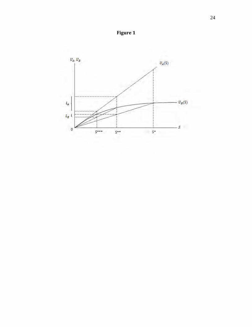
A and B have different risk preferences: A is risk neutral and B is risk averse.
More formally, the actors have respective utility functions ( ) and ( ) such that
( ) , ( ) > 0 and ( ) = 0, ( ) < 0. We also assume that (0) =
(0) = 0 and that the utility functions do not cross. This gives the two utility functions
shown in Figure 1.
Let [ ] = . Each actor receives utility from the asset, person A
receives ( ) = [ ( )], which can be seen in Figure 1 by tracing up from to
( ) and over to the vertical axis. B receives expected utility [ ( )], which can be
seen in Figure 1 by tracing up from to the ray connecting the origin to ( ) and
over to the vertical axis. Both actors are indifferent between going to court and a
settlement that gives them their expected utility of the risky asset, and will settle for that
amount or any greater amount. Person B is willing to accept a settlement of less than
due to risk aversion.4
4 The more risk averse actor accepting a smaller settlement appears in a more general case of two risk averse bargainers who will go to an uncertain arbitrator if they cannot reach a settlement by Crawford (1984). In Crawford’s model, an increase of an actor’s risk aversion leads to a decrease in their settlement all else equal.
There will then be age differences in settlement willingness to the
extent that risk aversion varies by age (Halek and Eisenhauer 2001, Anderson et al.
2008).
6
Now consider a cap on the amount that can be recovered in damages in a court
award. This will change the maximum amount of the risky asset. The new asset can
now either take on the value zero or with equal probability. Let [ ] = . We can
find each actor’s utility from the new asset in a similar fashion as before. Person A
receives ( ) = [ ( )], which can be seen in Figure 1 by tracing up from to
( ) and over to the vertical axis; B receives expected utility [ ( )], which can be
seen in Figure 1 by tracing up from to the ray connecting the origin to ( ) and
over to the vertical axis.
If we take the difference between the utility from the original asset , and the
capped asset we get for actor A, and for actor B. It is immediately noticeable
that > , or that the less risk averse actor has a larger reduction in utility from the
implementation of a cap on damages. The implication is that risk aversion differences by
age or predicted settlement size can lead to age and other differences in the welfare loss
from damage caps.
There are a few remarks that should be made about the above theoretical exercise.
The first is that the behavioral implications do not depend on one of the actors being risk
neutral. If actor A is also risk averse the result that the less risk averse party suffers a
larger utility loss is maintained as long as the other assumptions are still met. It is also
important to note that actors’ changes in minimum acceptable settlements do not follow
as clean a rule as their changes in utility. A careful inspection of Figure 1 may make it
look as if there is a clear association between changes in minimum acceptable settlement
and the relative risk aversion of the actors, but that is an artifice of A being risk neutral.
Any systematic effects of possible interpersonal differences in relative risk aversion and
7
their attendant implications for how damage caps affect the size (asset value) of the
settlement needs to be discovered empirically.
3. Data
The data we use to estimate the distributional consequences of malpractice
reforms come from the Texas Department of Insurance Closed Claims Database (CCD),
which include every insurance claim over $10,000 closed in Texas during 1988-2007.
The data include indications of the type of insurance and the party purchasing the
insurance so that one can identify cases that deal specifically with medical malpractice.
The subset of the data we use includes 21,733 claims on medical malpractice insurance
policies of health care providers including physicians, dentists, hospitals, and nursing
homes.
Each of our data points is a closed claim. Although there are data for 2007, there
can be cases originating prior to 2007 that closed after 2007 and so are not represented.
Each claim provides information on the time, location, and type of injury (the closed
claims report uses broad definitions such as brain damage or back injury rather than
diagnosis codes). For the injured party the data include age, employment status, and
availability of compensation other than torts. The CCD also has comprehensive
information concerning any and all legal action that took place including all settlement
amounts and jury awards. Finally there is limited information on the defendants,
including the type of entity plus information about the payout limits associated with its
policies, and the estimates of litigation and indemnity costs by its insurance providers.
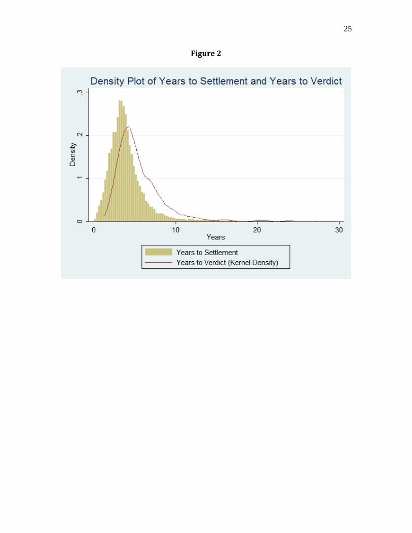
To ensure that we are not looking at people who are deliberately holding out for a
try at a so-called blockbuster jury award we limit our sample to cases settled in three
8
years or less (the average length of a case that reaches a verdict is 5.5 years).5
The main outcomes we examine are (1) the total amount of a settlement
conditional on settlement before a verdict, (2) the amount of compensation demanded by
the claimant conditional on settlement before a verdict, and (3) the time until settlement.
Because it is a claims database, the CCD contains plentiful information on the relevant
insurer and its behavior during the claims process. Of much importance is the indemnity
reserve, which is the amount of money that the insurance company has set aside to pay
for damages. The indemnity reserve is the insurance company’s best estimate of the risk
associated with a possible jury award or settlement, and effectively controls for many
characteristics of the injury. Last, the claims database that we use also contains
information on the specific policies’ per accident maximum payout limits.
The result
is a sample of 6,130 observations. Figure 2 shows the density of claims by year for both
settled claims and claims that go to verdict. By limiting our sample to three years we
exclude most cases that would have been settled close to verdict.
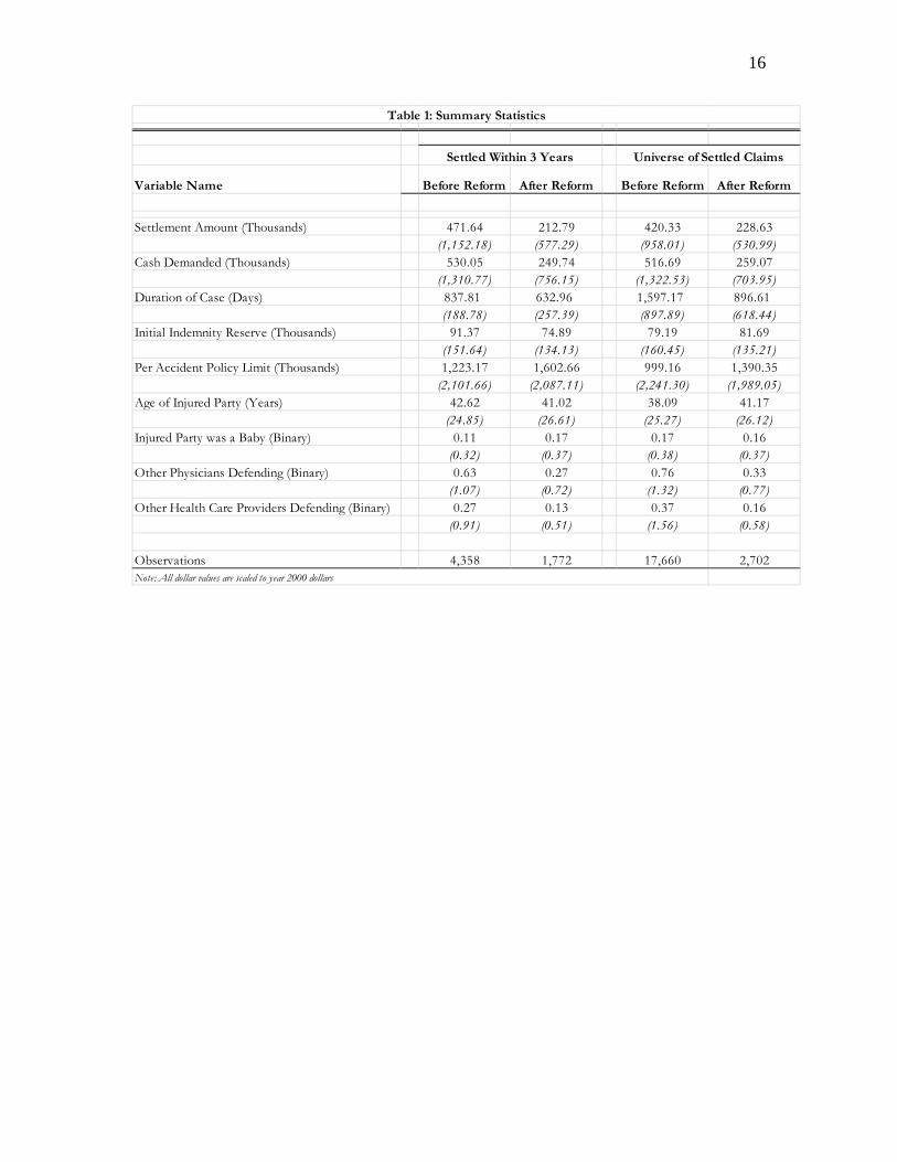
Table 1 contains the summary statistics for the data we use in the econometric
estimation to follow. The first row documents the substantial reduction (about 55 percent)
in the settlement amount after the reform, the second row documents a similar (50
percent) reduction in cash demanded, and the third row documents the notable reduction
(33-45 percent) in case duration. There is clear evidence that the Texas reforms affected
the ceiling of damages and encouraged quicker settlements on average. Our subsequent
econometric models clarify the distributional consequences and the channels at work in
the tort reforms producing the outcomes summarized in Table 1.
5 Later we examine the robustness of our results to the length of the settlement window.
9
4. Empirical Methods and Results
Estimating the component effects of the tort reform can be done with a multi-step
procedure. First we estimate the amount that average settlement compensation decreased
directly. Next we estimate the indirect effect in settlement amount via changes in cash
demanded. Finally, we estimate the reduction in time to settlement after the reform. In all
cases we consider distributional issues such as heterogeneity by age, settlement amounts
or time to settlement.
4.1 Settlement Amounts and Initial Cash Demanded
To begin to separate the direct and indirect effects of tort reform from other
variables that are also related to the size and speed of compensation, we estimate two
multivariate OLS regressions:
(1) Yit = 01 + 11X1it + 1Cit + 1Rt and
(2) Cit = 02 + 12 X2it + 2Rt.
Here Y is a claim settlement amount, X is a vector of time varying control variables
whose effect we wish to remove from our estimate of the effect of the reform, C is initial
cash demanded, and R is an indicator variable equal to one in the time period after the
reform has been enacted, and zero otherwise. Thus, k (k = 1, 2) is the estimated effect of
the reform on either the amount of the settlement or the amount initially demanded by the
claimant.
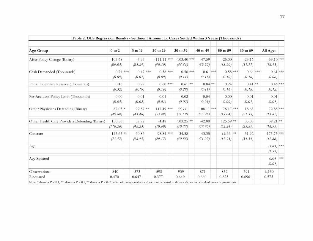
The OLS results in Table 2 illustrate the post-reform settlement amount holding
constant other factors, including cash demanded, which we view as an indicator of an
initial signal of how likely the claimant is willing to settle. The results for the all ages
regression reported in the last column indicate a $59,000 reduction in the settlement
10
amount post-reform, which is about 13 percent of the pre-reform mean. The
disaggregated results show that the groups most affected by the reform are people in the
20s and 30s, and that the reform is clearly non-neutral by age.
A final result of note in Table 2 is that for all the age groups there is a significant
effect of initial cash demanded on settlements, with the largest impact on babies, where
settlements rise by about $0.74 for every $1 of cash demanded initially. The consequence
is that one also need examine the effect of damage caps on the initial demands which, as
noted, may indicate bargaining rigidity of the claimant.
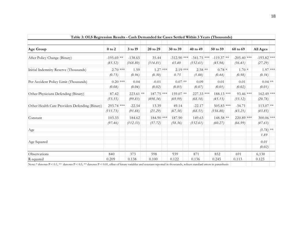
There is a substantial change in the post-reform period in initial cash demanded.
For the pooled (N = 6,130) regression in Table 3 there is about a 40 percent reduction in
initial cash demanded. So, when paired with the results of Table 2, the percentage total
effect of the reform, 100( 1 + 1 2)/ Y(pre-reform), is to reduce settlements by an average of
about 38 percent of the pre-reform average settlement, or by a total of $177,000. Once
again the results are heterogeneous by age, so that the largest dollar effects in Table 3 are
in the prime working years. This may indicate that working age people care about getting
back to work quickly compared to those close to retirement who may be more willing to
endure a protracted settlement period.
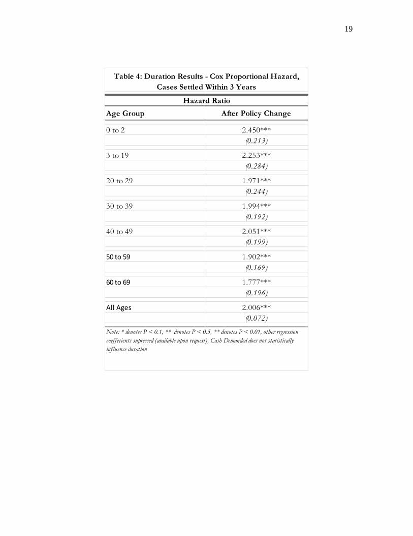
4.2 Time to Settlement
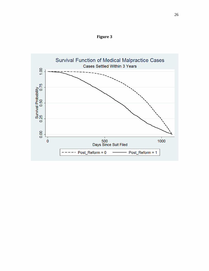
To examine the issue of how the reform affected time to payment we also
estimated Cox (1972) proportional hazard models
(3) hi(t) = h0(t)exp( 13Xit + 3Cit + 3Rt),
with standard errors calculated using the robust method in Lin and Wei (1979). Here the
antilog of the coefficient of the reform dummy implies the hazard ratios in Table 4, which
11
are revealed in the survival functions illustrated in Figure 3. Note, for example, that pre-
reform virtually no case had settled by the 500 day mark, while post-reform about one-
third had settled. Similarly, it took about 50 percent longer for half the cases to have
settled pre reform versus post reform.
From the estimated hazard ratios in Table 4 we see that, on average, people settle
about 50 percent faster with the largest effect ( 60 percent) on cases involving infants.
Again there is substantial heterogeneity in the estimated effect of the reform on time until
settlement, as cases involving the elderly are settled 40 percent more quickly. Finally, we
note that, unlike the level of settlements, time to settlement is not affected by initial cash
demanded so that there is no influence of the policy reform on time to settlement via a
moderation of cash demanded channel.
4.3 Effect of the Reform on the Economic Value of Settlements
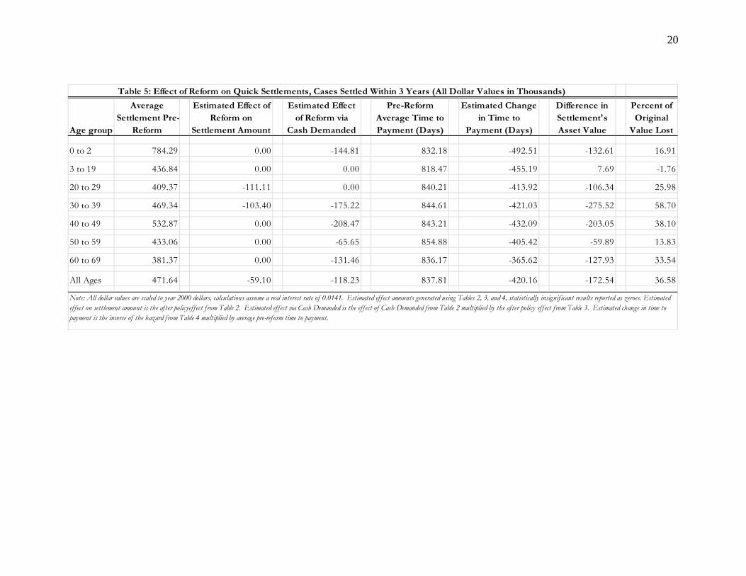
Using the procedure described in the Appendix we display in Table 5 the
economic effects of the reform in terms of its impact on the asset value of a malpractice
settlement. Table 5 breaks the effect of the policy out by channels, the direct effect on the
settlement amount, the indirect effect via decreased cash demands, and then the change in
timing from speedier settlements.
For all ages, while speeding up the time to payment by about 420 days, the effect
of reform on settlements is to reduce the present value by 36 percent.6
6 Present value calculations use the average of the real interest rate on a 3-month T-bill over the time period of our sample.
Once again there is
substantial heterogeneity by age. Persons in their 30s demand about $175,000 less and
then have an average settlement that is about $103,000 lower that is paid only about 421
days (50 percent) faster so that the implicit asset value of the settlement is about 60
12
percent ($276,000) lower. The tort reforms are not welfare improving in a basic
economic sense. One possible explanation for the heterogeneity by age is that claimants
in their prime working age have a different level of relative risk aversion than those with
injured children or the elderly. It is also possible that working age claimants settle for less
in an attempt to expedite the settlement process and return to work as quickly as possible.
4.4 Additional Dimensions of the Distributional Consequences of the Reform
There is much research demonstrating the usefulness of quantile regression in
examining the distributional consequences of economic interventions in the labor market
(Kniesner, Viscusi, and Ziliak 2010) and in the case of medical malpractice insurance
(Viscusi and Born 2005). The standard quantile regression model has an expression for
the fitted residual that in our case is
(4) = + + or
(5) = + .
Next there is a multiplier where
(6) = 2 , > 02(1 ),
with q the quantile of interest. The quantile regression is then
(7) | | ,
which is solved via linear programming (Armstrong, et al. 1975).
Recent research adds a parameter ( ) that, when minimized in conjunction with (4)-(7),
reveals the most probable or maximum entropy quantile (Golan 2006, Bera et al. 2010).7
7 One can also intuit as a penalty for deviating from the median as the most likely quantile.
13
In terms of policy interventions one should be particularly interested in the most likely
effect size, which comes from the most likely quantile.
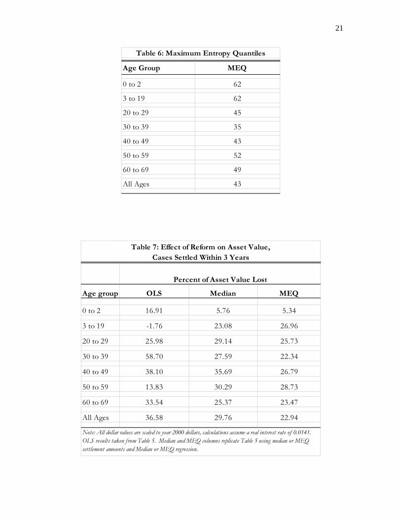
Table 6 presents the estimated maximum entropy quantile for the various age
groups. The point of the exercise is to reveal more of the policy heterogeneity. Note that
the estimated maximum entropy quantile is lower for older people. Although it is close to
the median for ages 50-69, in no other age group is the median outcome the place in the
fitted settlement distribution that is most likely.
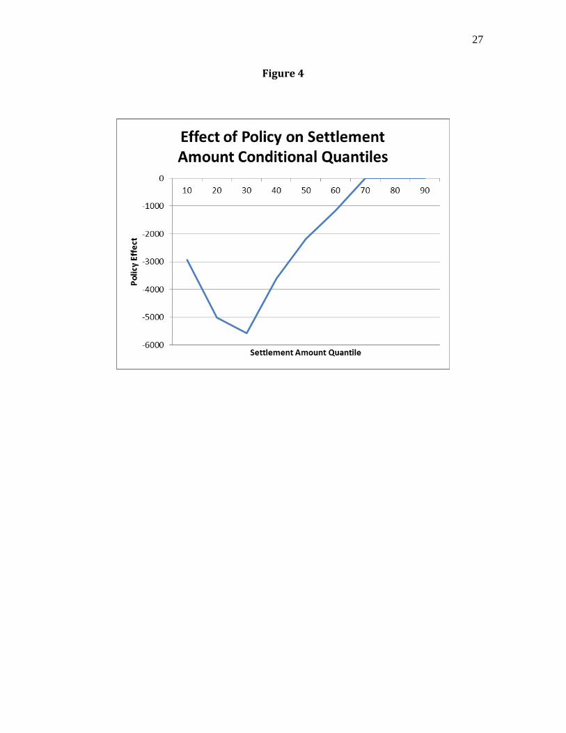
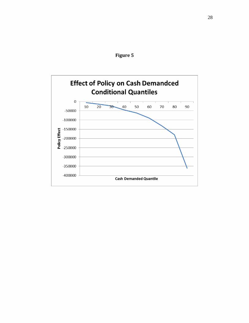
There is substantial heterogeneity in the impact of the reform across conditional
quantiles of cash demanded and settlement amounts. The differing effects of the policy
are presented in Figure 4 for conditional quantiles of settlement amount and in Figure 5
for conditional quantiles of cash demanded. For the pooled sample the negative effect of
the policy on settlement amounts peaks at the 30th conditional quantile and then drops off
at the quantiles increase. For cash demanded the effect of the policy is monotonically
increasing in magnitude with the conditional quantile. Because of the differing effects, if
a part of the distribution other than the mean is most likely, then using the estimated
policy effect at the maximum entropy quantile will make a sizable difference in the
estimated value of the settlement.
The heterogeneity in policy effects and the difference it makes in focusing on the
most likely place in the distribution of potential outcomes are highlighted in Table 7.
There we compare estimated mean, median, and maximum entropy quantile malpractice
reform effects on asset value lost. Note that for people in their 30s the most likely effect
is less than half the mean effect. Alternatively, the most likely effect is much larger ( 28
percent) than the mean effect (0) in the case of young people 3-19. It is also the case that
14
(1) there is little heterogeneity in effect by age group for the vast majority of the groups
and (2) the most likely quantile estimates are often fairly similar to the estimates one
would get from a median regression. When estimating medical malpractice reform
effects, a simple least absolute deviation regression, which trims the outliers, is an
important improvement over OLS.
The conclusion again emerging from maximum entropy quantile regressions is
that on pure economic asset returns grounds the policy is welfare reducing. Claimants
would have benefitted economically from a slower larger settlement typical of the pre-
reform period. Unlike what has been inferred previously (Finley 2004; Rubin and
Shepherd 2008), the results in Table 7 show that infants and the elderly are not the
hardest hit. In addition to infants having the smallest expected effects from damage caps
the largest percentage asset loss is among people in their 50s.
4.5 Robustness Check
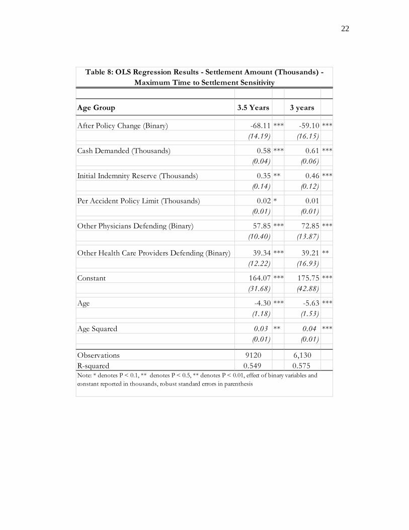
The final econometric issue we confront is whether our results are sensitive to
small changes in the assumed settlement period window of three years. Table 8 presents
settlement results for a 3.5 year time frame compared to a 3 year window, which enlarges
the sample size by 50 percent. Note the similarity of results of interest, the estimated
values of and , with those in Table 2.8
8 Results not tabulated are similar for settlement windows of 3.25 or 3.75 years.
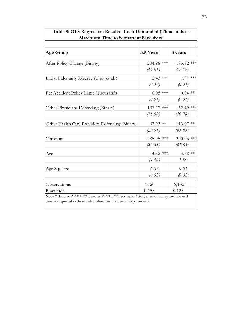
Table 9 repeats the robustness checking exercise
for the dependent variable of cash demanded by the claimant. Again, the results are
similar to those found in the three year window.
15
5. Conclusion
Because of its many perceived benefits state legislatures have found tort reform
attractive. Reforms such as damage caps and early offer systems speed up cases and help
reduce caseloads in the courts. They also lower the size of claims, which possibly
decreases so-called wasteful defensive medicine and decreases the related stress costs on
physicians. Another touted benefit of tort reforms are that they cut down on claims that
lack merit and help prevent blockbuster jury awards that are perceived to increase the
overall cost of health care. The benefits we have mentioned are not without a downside.
Our evidence is that although injured parties who may desire quicker payment are
compensated more quickly after the reforms, the cost of doing so is large. It may
certainly be the case that given the choice specified in clear economic terms claimants,
particularly those of prime working ages, would have preferred the pre-reform medical
malpractice tort system.
16
Variable Name Before Reform After Reform Before Reform After Reform
Settlement Amount (Thousands) 471.64 212.79 420.33 228.63(1,152.18) (577.29) (958.01) (530.99)
Cash Demanded (Thousands) 530.05 249.74 516.69 259.07(1,310.77) (756.15) (1,322.53) (703.95)
Duration of Case (Days) 837.81 632.96 1,597.17 896.61(188.78) (257.39) (897.89) (618.44)
Initial Indemnity Reserve (Thousands) 91.37 74.89 79.19 81.69(151.64) (134.13) (160.45) (135.21)
Per Accident Policy Limit (Thousands) 1,223.17 1,602.66 999.16 1,390.35(2,101.66) (2,087.11) (2,241.30) (1,989.05)
Age of Injured Party (Years) 42.62 41.02 38.09 41.17(24.85) (26.61) (25.27) (26.12)
Injured Party was a Baby (Binary) 0.11 0.17 0.17 0.16(0.32) (0.37) (0.38) (0.37)
Other Physicians Defending (Binary) 0.63 0.27 0.76 0.33(1.07) (0.72) (1.32) (0.77)
Other Health Care Providers Defending (Binary) 0.27 0.13 0.37 0.16(0.91) (0.51) (1.56) (0.58)
Observations 4,358 1,772 17,660 2,702
Table 1: Summary Statistics
Settled Within 3 Years Universe of Settled Claims
Note: All dollar values are scaled to year 2000 dollars
17
Age Group 0 to 2 3 to 19 20 to 29 30 to 39 40 to 49 50 to 59 60 to 69 All Ages
After Policy Change (Binary) -105.68 -4.95 -111.11 *** -103.40 *** -47.59 -25.00 -23.16 -59.10 ***(69.63) (63.84) (40.19) (35.54) (39.92) (18.20) (31.77) (16.15)
Cash Demanded (Thousands) 0.74 *** 0.47 *** 0.38 *** 0.56 *** 0.61 *** 0.55 *** 0.64 *** 0.61 ***(0.09) (0.07) (0.09) (0.14) (0.15) (0.10) (0.16) (0.06)
Initial Indemnity Reserve (Thousands) 0.46 0.29 0.60 *** 0.61 ** 0.84 ** 0.24 0.41 ** 0.46 ***(0.32) (0.19) (0.16) (0.29) (0.41) (0.16) (0.18) (0.12)
Per Accident Policy Limit (Thousands) 0.00 0.01 -0.01 0.02 0.04 0.00 -0.01 0.01(0.03) (0.02) (0.01) (0.02) (0.03) (0.00) (0.01) (0.01)
Other Physicians Defending (Binary) 87.03 * 99.57 ** 147.49 *** 35.14 108.11 *** 76.17 *** 18.63 72.85 ***(49.68) (43.46) (53.48) (31.59) (33.25) (19.04) (21.55) (13.87)
Other Health Care Providers Defending (Binary) 150.56 57.72 -4.48 103.25 ** -42.00 125.59 ** 35.08 39.21 **(110.26) (48.23) (10.69) (50.77) (37.70) (52.24) (23.87) (16.93)
Constant 143.63 ** 60.86 98.84 *** 34.58 -43.35 43.99 ** 31.92 175.75 ***(71.57) (98.45) (29.17) (30.85) (71.07) (17.93) (54.54) (42.88)
Age (5.63) ***(1.53)
Age Squared 0.04 ***(0.01)
Observations 840 373 598 939 871 852 691 6,130R-squared 0.470 0.647 0.377 0.640 0.660 0.823 0.696 0.575Note: * denotes P < 0.1, ** denotes P < 0.5, ** denotes P < 0.01, effect of binary variables and constant reported in thousands, robust standard errors in parenthesis
Table 2: OLS Regression Results - Settlment Amount for Cases Settled Within 3 Years (Thousands)
18
Age Group 0 to 2 3 to 19 20 to 29 30 to 39 40 to 49 50 to 59 60 to 69 All Ages
After Policy Change (Binary) -195.69 ** -138.65 35.44 -312.90 *** -341.75 *** -119.37 ** -205.40 *** -193.82 ***(85.52) (168.80) (114.81) 65.40 (152.61) (45.94) (36.41) (27.29)
Initial Indemnity Reserve (Thousands) 2.70 *** 1.59 1.27 *** 2.19 *** 2.58 ** 0.78 * 1.70 * 1.97 ***(0.73) (0.96) (0.30) 0.75 (1.00) (0.44) (0.98) (0.34)
Per Accident Policy Limit (Thousands) 0.20 *** 0.04 -0.01 0.07 ** 0.09 0.01 0.01 0.04 **(0.08) (0.04) (0.02) (0.03) (0.07) (0.01) (0.02) (0.01)
Other Physicians Defending (Binary) 87.42 223.61 ** 187.75 *** 159.07 ** 227.33 *** 188.13 *** 93.46 *** 162.49 ***(53.55) (99.83) (498.34) (69.99) (68.18) (45.13) (33.12) (20.78)
Other Health Care Providers Defending (Binary) 293.74 *** -22.54 13.39 49.14 -22.17 505.83 *** -34.71 113.07 **(111.73) (91.88) (21.29) (67.38) (68.51) (156.80) (43.21) (43.85)
Constant 103.33 184.62 184.90 *** 187.90 149.63 148.58 ** 220.89 *** 300.06 ***(97.46) (112.33) (37.72) (58.36) (152.61) (60.27) (66.99) (47.63)
Age (3.78) **1.89
Age Squared 0.01
(0.02)
Observations 840 373 598 939 871 852 691 6,130R-squared 0.209 0.138 0.100 0.122 0.136 0.245 0.113 0.123Note: * denotes P < 0.1, ** denotes P < 0.5, ** denotes P < 0.01, effect of binary variables and constant reported in thousands, robust standard errors in parenthesis
Table 3: OLS Regression Results - Cash Demanded for Cases Settled Within 3 Years (Thousands)
19
Age Group After Policy Change
0 to 2 2.450***(0.213)
3 to 19 2.253***(0.284)
20 to 29 1.971***(0.244)
30 to 39 1.994***(0.192)
40 to 49 2.051***(0.199)
50 to 59 1.902***(0.169)
60 to 69 1.777***(0.196)
All Ages 2.006***(0.072)
Table 4: Duration Results - Cox Proportional Hazard, Cases Settled Within 3 Years
Hazard Ratio
Note: * denotes P < 0.1, ** denotes P < 0.5, ** denotes P < 0.01, other regression
coef f ecients supressed (available upon request), Cash Demanded does not statistically
inf luence duration
20
Age group
Average Settlement Pre-
Reform
Estimated Effect of Reform on
Settlement Amount
Estimated Effect of Reform via
Cash Demanded
Pre-Reform Average Time to Payment (Days)
Estimated Change in Time to
Payment (Days)
Difference in Settlement's Asset Value
Percent of Original
Value Lost
0 to 2 784.29 0.00 -144.81 832.18 -492.51 -132.61 16.91
3 to 19 436.84 0.00 0.00 818.47 -455.19 7.69 -1.76
20 to 29 409.37 -111.11 0.00 840.21 -413.92 -106.34 25.98
30 to 39 469.34 -103.40 -175.22 844.61 -421.03 -275.52 58.70
40 to 49 532.87 0.00 -208.47 843.21 -432.09 -203.05 38.10
50 to 59 433.06 0.00 -65.65 854.88 -405.42 -59.89 13.83
60 to 69 381.37 0.00 -131.46 836.17 -365.62 -127.93 33.54
All Ages 471.64 -59.10 -118.23 837.81 -420.16 -172.54 36.58
Table 5: Effect of Reform on Quick Settlements, Cases Settled Within 3 Years (All Dollar Values in Thousands)
Note: All dollar values are scaled to year 2000 dollars, calculations assume a real interest rate of 0.0141. Estimated ef f ect amounts generated using Tables 2, 3, and 4, statistically insignif icant results reported as zeroes. Estimated
ef f ect on settlement amount is the af ter policyef f ect f rom Table 2. Estimated ef f ect via Cash Demanded is the ef f ect of Cash Demanded f rom Table 2 multiplied by the af ter policy ef f ect f rom Table 3. Estimated change in time to
payment is the inverse of the hazard f rom Table 4 multiplied by average pre-reform time to payment.
21
Age Group MEQ
0 to 2 62
3 to 19 62
20 to 29 45
30 to 39 35
40 to 49 43
50 to 59 52
60 to 69 49
All Ages 43
Table 6: Maximum Entropy Quantiles
Age group OLS Median MEQ
0 to 2 16.91 5.76 5.34
3 to 19 -1.76 23.08 26.96
20 to 29 25.98 29.14 25.73
30 to 39 58.70 27.59 22.34
40 to 49 38.10 35.69 26.79
50 to 59 13.83 30.29 28.73
60 to 69 33.54 25.37 23.47
All Ages 36.58 29.76 22.94
Table 7: Effect of Reform on Asset Value, Cases Settled Within 3 Years
Percent of Asset Value Lost
Note: All dollar values are scaled to year 2000 dollars, calculations assume a real interest rate of 0.0141.
OLS results taken f rom Table 5. Median and MEQ columns replicate Table 5 using median or MEQ
settlement amounts and Median or MEQ regression.
22
Age Group 3.5 Years 3 years
After Policy Change (Binary) -68.11 *** -59.10 ***(14.19) (16.15)
Cash Demanded (Thousands) 0.58 *** 0.61 ***(0.04) (0.06)
Initial Indemnity Reserve (Thousands) 0.35 ** 0.46 ***(0.14) (0.12)
Per Accident Policy Limit (Thousands) 0.02 * 0.01(0.01) (0.01)
Other Physicians Defending (Binary) 57.85 *** 72.85 ***(10.40) (13.87)
Other Health Care Providers Defending (Binary) 39.34 *** 39.21 **(12.22) (16.93)
Constant 164.07 *** 175.75 ***(31.68) (42.88)
Age -4.30 *** -5.63 ***(1.18) (1.53)
Age Squared 0.03 ** 0.04 ***(0.01) (0.01)
Observations 9120 6,130R-squared 0.549 0.575
Table 8: OLS Regression Results - Settlement Amount (Thousands) - Maximum Time to Settlement Sensitivity
Note: * denotes P < 0.1, ** denotes P < 0.5, ** denotes P < 0.01, effect of binary variables and constant reported in thousands, robust standard errors in parenthesis
23
Age Group 3.5 Years 3 years
After Policy Change (Binary) -204.98 *** -193.82 ***(43.81) (27.29)
Initial Indemnity Reserve (Thousands) 2.43 *** 1.97 ***(0.39) (0.34)
Per Accident Policy Limit (Thousands) 0.05 *** 0.04 **(0.01) (0.01)
Other Physicians Defending (Binary) 137.72 *** 162.49 ***(18.00) (20.78)
Other Health Care Providers Defending (Binary) 67.93 ** 113.07 **(29.01) (43.85)
Constant 285.95 *** 300.06 ***(43.81) (47.63)
Age -4.32 *** -3.78 **(1.56) 1.89
Age Squared 0.02 0.01
(0.02) (0.02)
Observations 9120 6,130R-squared 0.153 0.123
Table 9: OLS Regression Results - Cash Demanded (Thousands) - Maximum Time to Settlement Sensitivity
Note: * denotes P < 0.1, ** denotes P < 0.5, ** denotes P < 0.01, effect of binary variables and constant reported in thousands, robust standard errors in parenthesis
24
Figure 1
25
Figure 2
26
Figure 3
27
Figure 4
28
Figure 5
29
References
Abraham, K. S. (2001). “The Trouble with Negligence.” Vanderbilt Law Review 54(3):
1187-1224.
Anderoni, J. and C. Sprenger. (2010). “Risk Preferences are not Time Preferences:
Discounted Expected Utility with a Disproportionate Preference for Certainty.”
National Bureau of Economic Research, Working Paper 16348.
Andersen, S., G. W. Harrison, M. I. Lau, and E. E. Rutström. (2008). “Eliciting Risk and
Time Preferences.” Econometrica 76(3): 583-618.
Armstrong, R. D., E. L. Frome, and D. S. Kung. (1979). “Algorithm 79-01: A Revised
Simplex Algorithm for the Absolute Curve Fitting Problem.” Communications in
Statistics, Simulation and Computation 8: 175-190.
Avraham, R. (2007). “An Empirical Study of the Impact of Tort Reforms on Medical
Malpractice Settlement Payments.” Journal of Legal Studies 36(S2): S183-S229.
Baicker, K. and A. Chandra. (2006). “The Labor Market Effects of Rising Health
Insurance Premiums.” Journal of Labor Economics 24(3): 609-634.
Becker, G.S. and C. B. Mulligan. (1997). “The Endogenous Determination of Time
Preference.” The Quarterly Journal of Economics 112(3): 729-758.
Bera, A. K., A. F. Galvao Jr., G. V. Montes-Rojas, and S. Y. Park. (2010). “Which
Quantile is the Most Informative? Maximum Likelihood, Maximum Entropy and
Quantile Regression.” Working Paper, Department of Economics, University of
Illinois.
30
Black, B., D. A. Hyman, and C. Silver (2009), “The Effects of ‘Early Offers’ in Medical
Malpractice Cases: Evidence from Texas.” Journal of Empirical Legal Studies
6(4): 723-767.
Cox, D. R. (1972). “Regression Models and Life-Tables (with discussion).” Journal of
the Royal Statistical Society, Series B 34:187-220.
Crawford, V. P. (1982). “Compulsory Arbitration, Arbitral Risk and Negotiated
Settlements: A Case Study in Bargaining Under Imperfect Information.” The
Review of Economic Studies 49(1): 69-82.
Danzon, P. M. (1985). Medical Malpractice. Cambridge: Harvard University Press.
Donohue, J. J. and D. E. Ho. (2007). “The Impact of Damage Caps on Malpractice
Claims: Randomization Inferences with Difference-in-Differences.” Journal of
Empirical Legal Studies 4(1): 69-102.
Finley, L. M. (2004). “The Hidden Victims of Tort Reform: Women, Children, and the
Elderly.” Emory Law Journal 53(3): 1263-1314.
Golan, A. (2006). “Information and Entropy Econometrics – A Review and Synthesis.”
Foundations and Trends in Econometrics. 2(1-2).
Halek, M. and J. G. Eisenhauer. (2001). “Demography of Risk Aversion.” Journal of Risk
and Insurance 68(1): 1-24.
Hersch, J., J. O’Connell, and W. K. Viscusi. (2007). “An Empirical Assessment of Early
Offer Reform for Medical Malpractice.” Journal of Legal Studies 36(S2): S231-
S256.
31
Hyman, D. A., B. Black, C. Silver, and W. M. Sage (2009), “Estimating the Effect of
Damages Caps in Medical Malpractice Cases: Evidence from Texas.” Journal of
Legal Analysis 1(1): 355-409.
Keenan, D. C., D. C. Rudow, and A. Snow. (2008). “Risk Preferences and Changes in
Background Risk.” Journal of Risk and Uncertainty 36(2): 139-152.
Kessler, D. P. (2011). “Evaluating the Medical Malpractice System and Options for
Reform.” Journal of Economic Perspectives 25(2): 93-110.
Kessler, D. P. and M. McClellan. (1996). “Do Doctors Practice Defensive Medicine?”
Quarterly Journal of Economics 111(2): 353-390.
Kessler, D. P., W. M. Sage, and D. J. Becker. (2005). “Impact of Malpractice Reforms on
the Supply of Physician Services.” Journal of the American Medical Association
293(21): 1831-1834.
Kim, B. (2007). “The Impact of Malpractice Risk on the Use of Obstetrics Procedures.”
Journal of Legal Studies 36(2): 79-116.
Kniesner, T. J., W. K. Viscusi, and J. P. Ziliak. (2010). “Policy Relevant Heterogeneity in
the Value of a Statistical Life: New Evidence from Panel Data Quantile
Regressions.” Journal of Risk and Uncertainty 40(1): 15-32.
Lakdawalla, D. N. and S. A. Seabury. (2009). “The Welfare Effects of Medical
Malpractice Liability.” National Bureau of Economic Research, Working Paper
15383.
Lin, D. Y. and L.J. Wei. (1989). “The Robust Inference for the Cox Proportional Hazards
Model,” Journal of the American Statistical Association 84: 1074-1078.
32
Matsa, D. A. (2007). “Does Malpractice Liability Keep the Doctor Away? Evidence from
Tort Reform Damage Caps.” Journal of Legal Studies 36(2): 143-230.
Mello, M. M., A. Chandra, A. A. Gawande, and D. M. Studdert. (2010). “National Costs
of the Medical Liability System.” Health Affairs 29(9): 1569-1577.
Rubin, P. H., and J. M. Shepherd. (2008). “The Demographics of Tort Reform.” Review
of Law and Economics 4(2): 591-620.
Sloan, F. A., and L. M. Chepke. (2008). Medical Malpractice. Cambridge: The MIT
Press.
Sloan, F. A., P. M. Mergenhagen, and R. R. Bovbjerg. (1989). “Effects of Tort Reforms
on the Value of Closed Medical Malpractice Claims: A Microanalysis.” Journal
of Health Politics, Policy and Law 14(4): 663-689.
Sunstein, C. R., R. Hastie, J. W. Payne, D. A. Schkade and W. K. Viscusi. (2002).
Punitive Damages, How Juries Decide. Chicago: The University of Chicago
Press.
Viscusi, W. K. (1991). Reforming Products Liability. Cambridge: Harvard University
Press.
Viscusi, W. K. and P. H. Born (2005). “Damages Caps, Insurability, and the Performance
of Medical Malpractice Insurance.” Journal of Risk and Uncertainty 72(1): 23-
43.
33
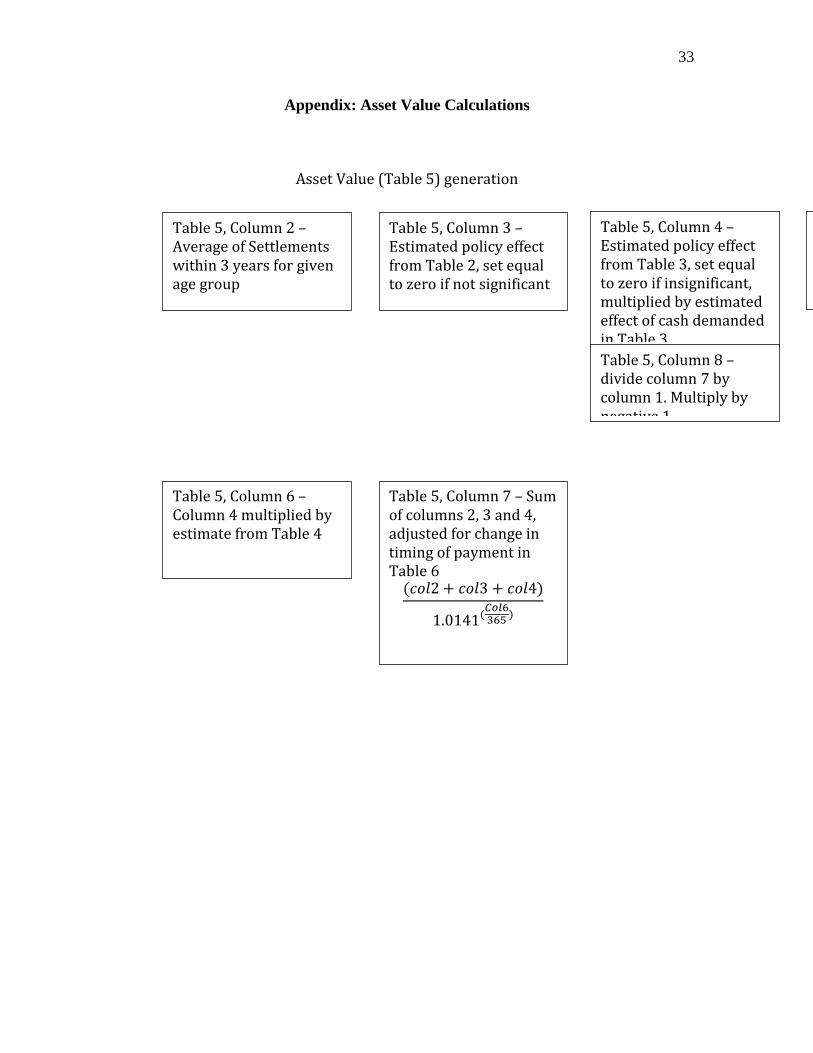
Appendix: Asset Value Calculations
Asset Value (Table 5) generation
Table 5, Column 2 – Average of Settlements within 3 years for given age group
Table 5, Column 3 – Estimated policy effect from Table 2, set equal to zero if not significant
Table 5, Column 4 – Estimated policy effect from Table 3, set equal to zero if insignificant, multiplied by estimated effect of cash demanded in Table 3
Table 5, Column 5 – Average duration of case in pre-‐policy period
Table 5, Column 6 – Column 4 multiplied by estimate from Table 4
( 2 + 3 + 4)1.0141( )
Table 5, Column 7 – Sum of columns 2, 3 and 4, adjusted for change in timing of payment in Table 6
Table 5, Column 8 – divide column 7 by column 1. Multiply by negative 1
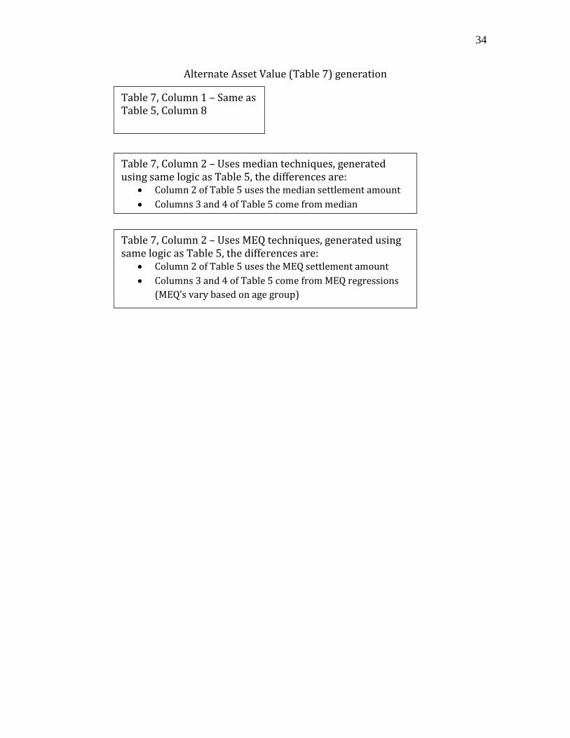
34
Alternate Asset Value (Table 7) generation
Table 7, Column 1 – Same as Table 5, Column 8
Table 7, Column 2 – Uses median techniques, generated using same logic as Table 5, the differences are:
Column 2 of Table 5 uses the median settlement amount Columns 3 and 4 of Table 5 come from median
Table 7, Column 2 – Uses MEQ techniques, generated using same logic as Table 5, the differences are:
Column 2 of Table 5 uses the MEQ settlement amount Columns 3 and 4 of Table 5 come from MEQ regressions (MEQ’s vary based on age group)