Embed Size (px)
Citation preview
THE DISAPPEARANCE OF
FUSION-FISSION AND THE ONSET OF
MULTIFRAGMENTATION
by
EUGENE EDWARD GUALTIERI
A DISSERTATION
Submitted to
Michigan State University
in partial ful�llment of the requirements
for the Degree of
DOCTOR OF PHILOSOPHY
Department of Physics and Astronomy
1995
ABSTRACT
THE DISAPPEARANCE OF FUSION-FISSION AND THE ONSET OF
MULTIFRAGMENTATION
By
Eugene Edward Gualtieri
Information about the evolution of momentum transfer and excitation energy in
intermediate energy heavy ion collisions of a �ssile target was extracted through an
analysis of �ssion fragment folding angles and charged particle production as beam
energy is increased. An exclusive measurement of central events is performed using
the MSU 4� Array as an impact parameter �lter. For central collisions, a saturation is
found in linear momentum transfer but evidence is presented that excitation energy
increases steadily with beam energy. The implications of these measurements are
discussed.
The space time aspects of the collisions are probed using an analysis which is
sensitive to the shape of the ellipsoidal ow envelope of the reaction products in
momentum space. This event shape analysis is used to determine whether the dom-
inant reaction mechanism is of a sequential-binary or simultaneous nature and was
performed in order to determine at what energy the multifragmentation channel be-
comes the dominant mode of decay. Such a transition is expected to occur when the
excitation energy of the system approaches that of the total binding energy of the
system. We deduce that 55 AMeV is the lower limit of the bombarding energy at
which multifragmentation becomes dominant in this system.

For Mary
iii

ACKNOWLEDGEMENTS
Here I sit, actually writing the acknowledgements page of my dissertation. I have
been dreaming about this for �ve years. Of course, in order to actually reach this
point, I needed the help of several people and I would like to thank them here.
First I must thank my parents, Edward and Lola Gualtieri, who taught me the
basic values that helped me to persevere and �nish this program. They experienced
the ups and downs of a graduate student's life right along with me.
My deepest thanks go to my advisor, Gary Westfall. How he put up with such
a paranoid graduate student I will never know. His con�dence in me �lled in when
my own self-con�dence waned, and kept me on track toward my degree. Gary's
enthusiasm for his work and for the accomplishments of his colleagues is a great
source of inspiration and something I admire greatly. I will consider myself a success
if I can give to just one person what Gary has given me.
Working with Skip Vander Molen has been both a pleasure and a privilege. He
is incredibly dedicated to his work, and more than willing to go above and beyond
the call of duty in order to ensure the success of an experiment. I owe a great deal
of what I know about nuclear electronics to time spent in the vault with Skip and an
oscilloscope.
The post-docs that have come and gone during my time with the 4� group { Roy
Lacey, Sherry Yennello, and Bill Llope { have all provided invaluable guidance and
advice. Though their styles and personalities di�ered, they all shared a real devotion
to their work and were all willing to take the time to help me and other graduate
students. From their examples, I learned what qualities are necessary in order to
succeed.
iv
A huge \thank you" goes to my fellow graduate students in the 4� group: Stefan
Hannuschke, Robert Pak, Nathan Stone, and Jaeyong Yee. One of the greatest
joys in my graduate career has been working in collaboration with them on physics
experiments. When it came time to run my thesis experiment it was reassuring to
know that they were there to back me up at 3:00 in the morning.
Special thanks go to Salvatore Fahey, my friend and partner during the �rst two
years of classes and the candidacy exam. The memory of the expression on Sal's face
as we opened the results of that exam is indelibly etched in my mind, and kept me
going whenever I was frustrated or depressed.
Finally, I must thank my wife, Mary McManus. I could not have made it through
this program without her unconditional support and tireless faith in me. Although
she was struggling along the same path as I, in pursuit of her own degree, she was
absolutely sel ess in her support of me, and was always there whenever I needed her
to listen.
v

vi
Contents
LIST OF TABLES ix
LIST OF FIGURES x
1 Introduction 1
2 Experimental Details 11
2.1 Introduction : : : : : : : : : : : : : : : : : : : : : : : : : : : : : : : : 11
2.2 Michigan State University 4� Array : : : : : : : : : : : : : : : : : : : 12
2.2.1 Plastic Phoswich Counters : : : : : : : : : : : : : : : : : : : : 12
2.2.2 Bragg Curve Counters : : : : : : : : : : : : : : : : : : : : : : 24
2.2.3 Multi-Wire Proportional Counters : : : : : : : : : : : : : : : : 31
3 Momentum Transfer and Deposited Energy 41
3.1 Introduction : : : : : : : : : : : : : : : : : : : : : : : : : : : : : : : : 41
3.2 Folding Angle Distributions : : : : : : : : : : : : : : : : : : : : : : : 41
3.3 Azimuthal Distributions : : : : : : : : : : : : : : : : : : : : : : : : : 48
3.4 IMF and LCP Production : : : : : : : : : : : : : : : : : : : : : : : : 50
3.5 Calculations of Momentum Transfer and Excitation Energy : : : : : : 57
3.5.1 Linear Momentum Transfer : : : : : : : : : : : : : : : : : : : 57
3.5.2 Excitation Energy : : : : : : : : : : : : : : : : : : : : : : : : : 61
3.6 Summary and Discussion : : : : : : : : : : : : : : : : : : : : : : : : : 64
4 Event Shape Analysis 67
4.1 Introduction : : : : : : : : : : : : : : : : : : : : : : : : : : : : : : : : 67
4.2 The Flow Tensor : : : : : : : : : : : : : : : : : : : : : : : : : : : : : 67
4.2.1 Sphericity and Coplanarity : : : : : : : : : : : : : : : : : : : : 70
4.3 Relationship of the Event Shape to the Reaction Mechanism : : : : : 72
4.4 E�ects Which May Distort the Event Shape : : : : : : : : : : : : : : 74
vii
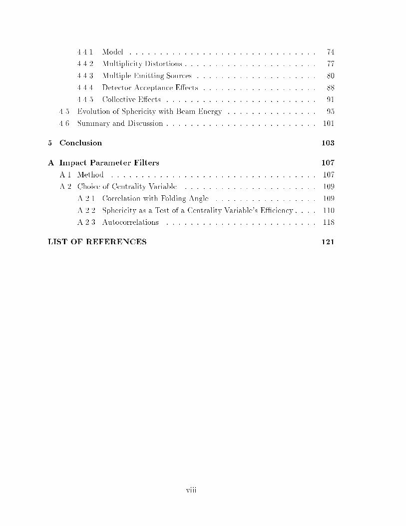
4.4.1 Model : : : : : : : : : : : : : : : : : : : : : : : : : : : : : : : 74
4.4.2 Multiplicity Distortions : : : : : : : : : : : : : : : : : : : : : : 77
4.4.3 Multiple Emitting Sources : : : : : : : : : : : : : : : : : : : : 80
4.4.4 Detector Acceptance E�ects : : : : : : : : : : : : : : : : : : : 88
4.4.5 Collective E�ects : : : : : : : : : : : : : : : : : : : : : : : : : 91
4.5 Evolution of Sphericity with Beam Energy : : : : : : : : : : : : : : : 95
4.6 Summary and Discussion : : : : : : : : : : : : : : : : : : : : : : : : : 101
5 Conclusion 103
A Impact Parameter Filters 107
A.1 Method : : : : : : : : : : : : : : : : : : : : : : : : : : : : : : : : : : 107
A.2 Choice of Centrality Variable : : : : : : : : : : : : : : : : : : : : : : 109
A.2.1 Correlation with Folding Angle : : : : : : : : : : : : : : : : : 109
A.2.2 Sphericity as a Test of a Centrality Variable's E�ciency : : : : 110
A.2.3 Autocorrelations : : : : : : : : : : : : : : : : : : : : : : : : : 118
LIST OF REFERENCES 121
viii
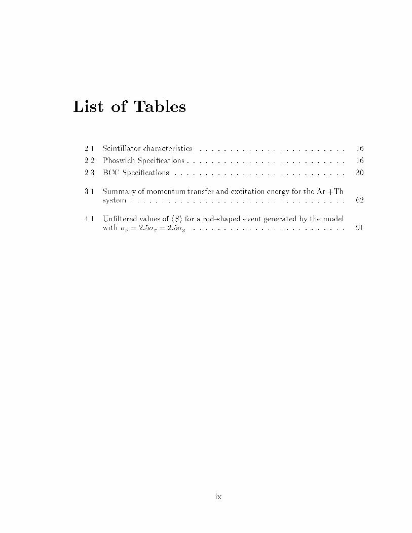
List of Tables
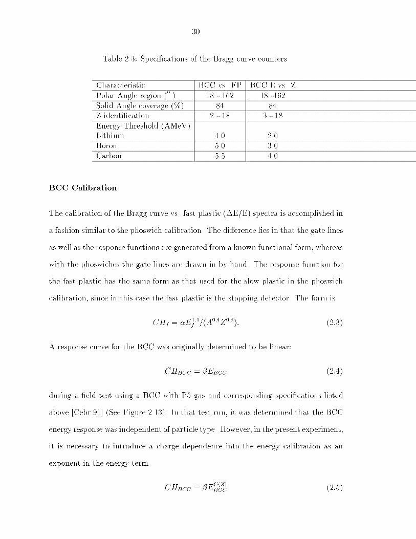
2.1 Scintillator characteristics : : : : : : : : : : : : : : : : : : : : : : : : 16
2.2 Phoswich Speci�cations : : : : : : : : : : : : : : : : : : : : : : : : : : 16
2.3 BCC Speci�cations : : : : : : : : : : : : : : : : : : : : : : : : : : : : 30
3.1 Summary of momentum transfer and excitation energy for the Ar +Thsystem. : : : : : : : : : : : : : : : : : : : : : : : : : : : : : : : : : : : 62
4.1 Un�ltered values of hSi for a rod-shaped event generated by the modelwith �z = 2:5�x = 2:5�y. : : : : : : : : : : : : : : : : : : : : : : : : : 91
ix

x
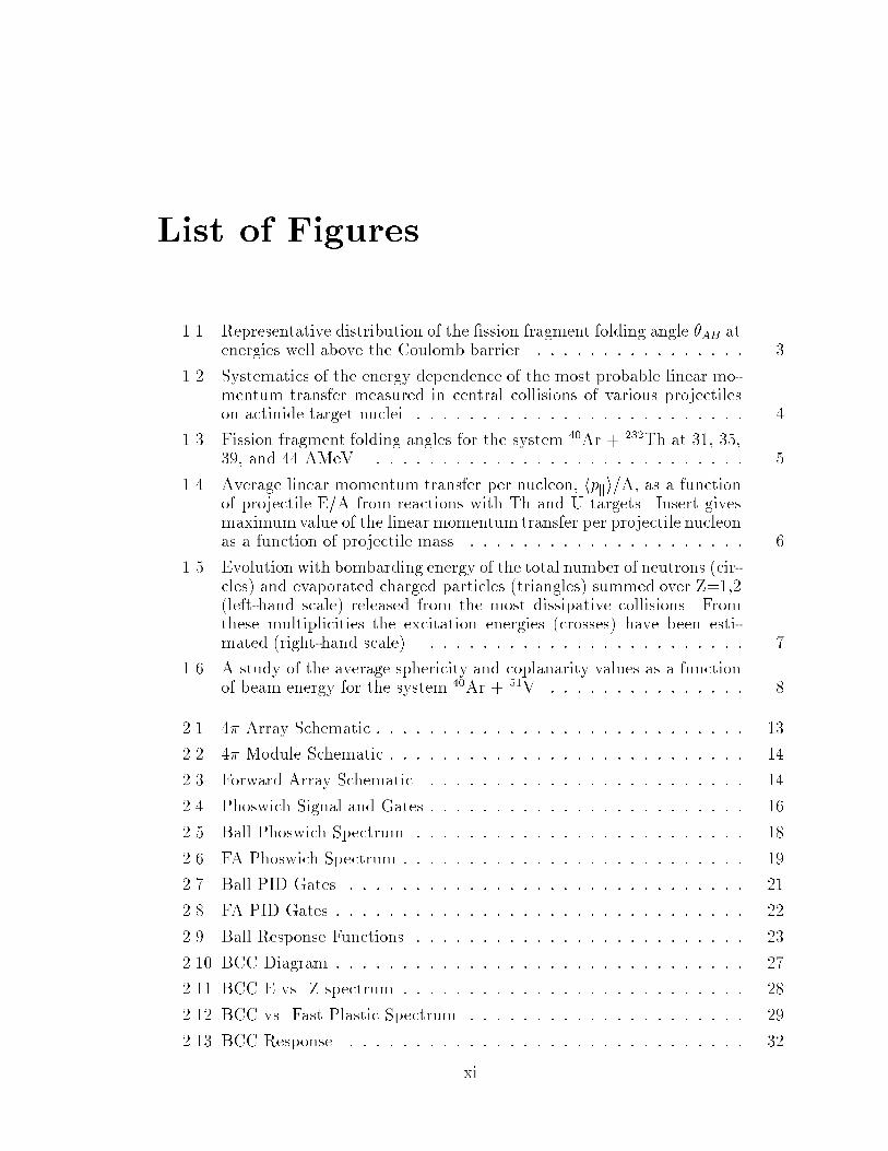
List of Figures
1.1 Representative distribution of the �ssion fragment folding angle �AB atenergies well above the Coulomb barrier. : : : : : : : : : : : : : : : : 3
1.2 Systematics of the energy dependence of the most probable linear mo-mentum transfer measured in central collisions of various projectileson actinide target nuclei. : : : : : : : : : : : : : : : : : : : : : : : : : 4
1.3 Fission fragment folding angles for the system 40Ar + 232Th at 31, 35,39, and 44 AMeV. : : : : : : : : : : : : : : : : : : : : : : : : : : : : 5
1.4 Average linear momentum transfer per nucleon, hpki/A, as a functionof projectile E/A from reactions with Th and U targets. Insert givesmaximumvalue of the linear momentum transfer per projectile nucleonas a function of projectile mass. : : : : : : : : : : : : : : : : : : : : : 6
1.5 Evolution with bombarding energy of the total number of neutrons (cir-cles) and evaporated charged particles (triangles) summed over Z=1,2(left-hand scale) released from the most dissipative collisions. Fromthese multiplicities the excitation energies (crosses) have been esti-mated (right-hand scale). : : : : : : : : : : : : : : : : : : : : : : : : 7
1.6 A study of the average sphericity and coplanarity values as a functionof beam energy for the system 40Ar + 51V. : : : : : : : : : : : : : : : 8
2.1 4� Array Schematic : : : : : : : : : : : : : : : : : : : : : : : : : : : : 13
2.2 4� Module Schematic : : : : : : : : : : : : : : : : : : : : : : : : : : : 14
2.3 Forward Array Schematic : : : : : : : : : : : : : : : : : : : : : : : : 14
2.4 Phoswich Signal and Gates : : : : : : : : : : : : : : : : : : : : : : : : 16
2.5 Ball Phoswich Spectrum : : : : : : : : : : : : : : : : : : : : : : : : : 18
2.6 FA Phoswich Spectrum : : : : : : : : : : : : : : : : : : : : : : : : : : 19
2.7 Ball PID Gates : : : : : : : : : : : : : : : : : : : : : : : : : : : : : : 21
2.8 FA PID Gates : : : : : : : : : : : : : : : : : : : : : : : : : : : : : : : 22
2.9 Ball Response Functions : : : : : : : : : : : : : : : : : : : : : : : : : 23
2.10 BCC Diagram : : : : : : : : : : : : : : : : : : : : : : : : : : : : : : : 27
2.11 BCC E vs. Z spectrum : : : : : : : : : : : : : : : : : : : : : : : : : : 28
2.12 BCC vs. Fast Plastic Spectrum : : : : : : : : : : : : : : : : : : : : : 29
2.13 BCC Response : : : : : : : : : : : : : : : : : : : : : : : : : : : : : : 32
xi
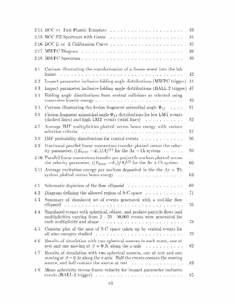
2.14 BCC vs. Fast Plastic Template : : : : : : : : : : : : : : : : : : : : : 33
2.15 BCC EZ Spectrum with Gates. : : : : : : : : : : : : : : : : : : : : : 34
2.16 BCC E vs. Z Calibration Curve : : : : : : : : : : : : : : : : : : : : : 35
2.17 MWPC Diagram : : : : : : : : : : : : : : : : : : : : : : : : : : : : : 38
2.18 MWPC Spectrum : : : : : : : : : : : : : : : : : : : : : : : : : : : : : 39
3.1 Cartoon illustrating the transformation of a �ssion event into the labframe. : : : : : : : : : : : : : : : : : : : : : : : : : : : : : : : : : : : 42
3.2 Impact parameter inclusive folding angle distributions (MWPC trigger) 44
3.3 Impact parameter inclusive folding angle distributions (BALL 2 trigger) 47
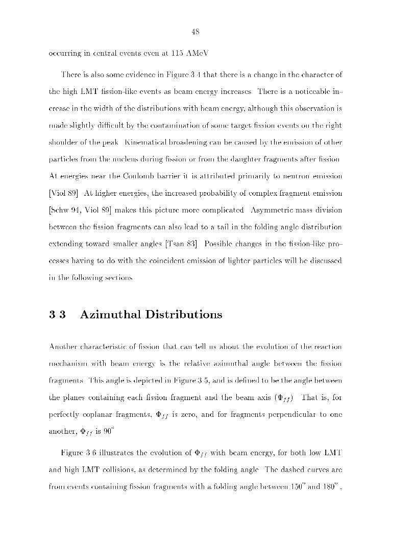
3.4 Folding angle distributions from central collisions as selected usingtransverse kinetic energy. : : : : : : : : : : : : : : : : : : : : : : : : : 49
3.5 Cartoon illustrating the �ssion fragment azimuthal angle �ff . : : : : 51
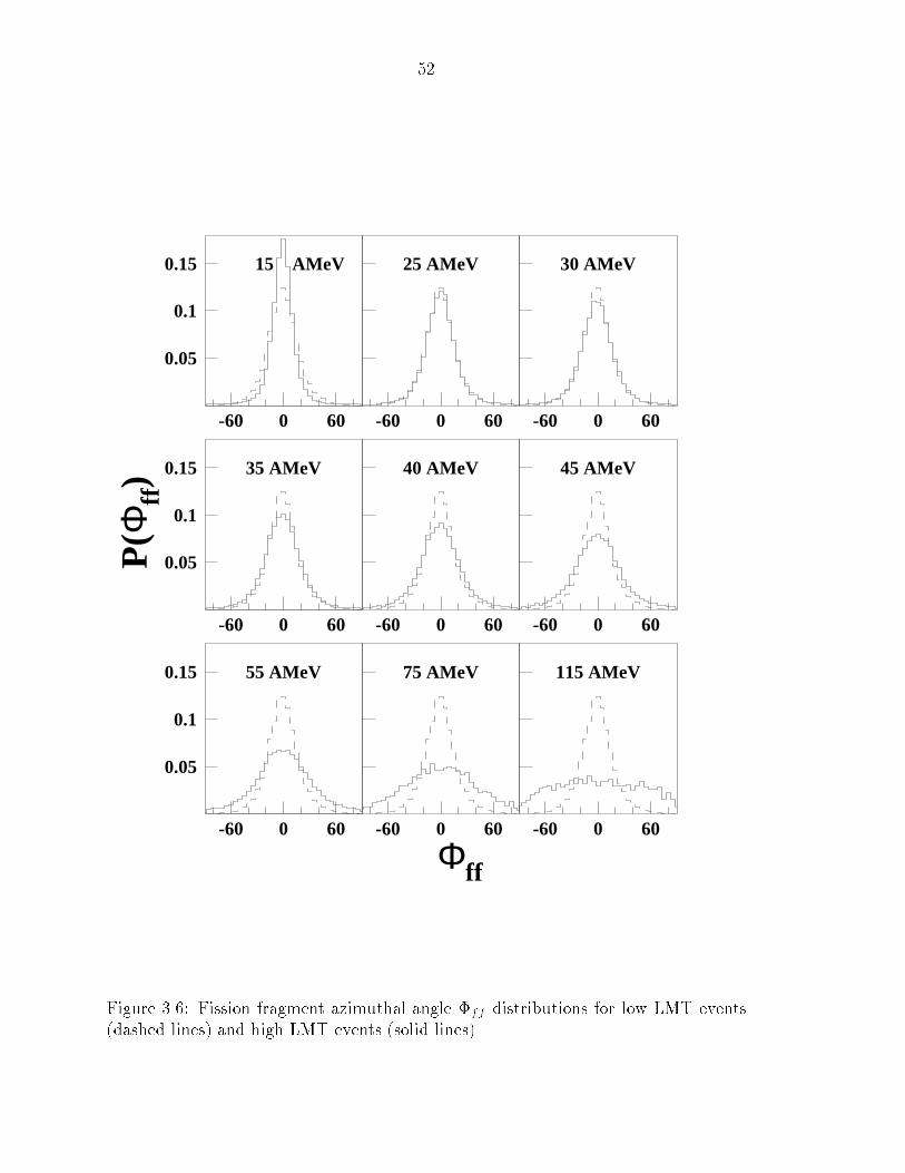
3.6 Fission fragment azimuthal angle �ff distributions for low LMT events(dashed lines) and high LMT events (solid lines). : : : : : : : : : : : 52
3.7 Average IMF multiplicities plotted versus beam energy with variousselection criteria. : : : : : : : : : : : : : : : : : : : : : : : : : : : : : 54
3.8 IMF probability distributions for central events. : : : : : : : : : : : : 56
3.9 Fractional parallel linear momentum transfer plotted versus the veloc-ity parameter, ((Ebeam � Ec)=A)
1=2 for the Ar +Th system. : : : : : : 59
3.10 Parallel linear momentumtransfer per projectile nucleon plotted versusthe velocity parameter, ((Ebeam � Ec)=A)
1=2 for the Ar +Th system. : 60
3.11 Average excitation energy per nucleon deposited in the the Ar + Thsystem plotted versus beam energy. : : : : : : : : : : : : : : : : : : : 63
4.1 Schematic depiction of the ow ellipsoid. : : : : : : : : : : : : : : : : 69
4.2 Diagram de�ning the allowed region of S-C space. : : : : : : : : : : : 71
4.3 Summary of simulated set of events generated with a rod-like owellipsoid. : : : : : : : : : : : : : : : : : : : : : : : : : : : : : : : : : : 76
4.4 Simulated events with spherical, oblate, and prolate particle ows andmultiplicities varying from 2 - 20. 50,000 events were generated foreach multiplicity and shape. : : : : : : : : : : : : : : : : : : : : : : : 78
4.5 Contour plot of the area of S-C space taken up by central events forall nine energies studied. : : : : : : : : : : : : : : : : : : : : : : : : : 79
4.6 Results of simulation with two spherical sources in each event, one atrest and one moving at � = 0.2c along the z-axis. : : : : : : : : : : : 82
4.7 Results of simulation with two spherical sources, one at rest and onemoving at � = 0.2c along the z-axis. Half the events contain the movingsource, and half contain the source at rest. : : : : : : : : : : : : : : : 83
4.8 Mean sphericity versus frame velocity for impact parameter inclusiveevents (BALL-2 trigger). : : : : : : : : : : : : : : : : : : : : : : : : : 85
xii
4.9 Mean sphericity versus frame velocity for the 10% most central eventsas determined using total transverse charge (ZT ). The ow tensornormalization constant used is 1
2m. : : : : : : : : : : : : : : : : : : : 87
4.10 Mean sphericity versus frame velocity for the 10% most central eventsas determined using total transverse charge (ZT ). The ow tensornormalization constant used is 1
p2. : : : : : : : : : : : : : : : : : : : : 89
4.11 Mean sphericity versus beam energy for 9 event sets each generatedwith a spherical ow ellipsoid, and boosted to one of the center-of-mass velocities corresponding to the 9 beam energies. The data wasthen �ltered through a software replica of the 4� Array. : : : : : : : : 92
4.12 Sphericity probability distribution for events with multiplicity Nc = 10,from experimental data, un�ltered simulation, and �ltered simulation. 93
4.13 Mean sphericity versus beam energy for 9 event sets each generatedwith a rod-like ow ellipsoid, and boosted to one of the center-of-massvelocities corresponding to the 9 beam energies. The data was then�ltered through a software replica of the 4� Array. : : : : : : : : : : : 94
4.14 Mean values of sphericity plotted versus charged particle multiplicity(Nc), for four incident beam energies of 40Ar + 232Th. : : : : : : : : : 96
4.15 Mean sphericity versus beam energy for central collisions as determinedusing total transverse charge (ZT ). Fission fragments not included. : : 98
4.16 Mean sphericity versus beam energy for central collisions as determinedusing total transverse charge (ZT ). Fission fragments included. : : : : 99
4.17 Mean sphericity versus beam energy for central collisions as determinedusing total transverse charge (ZT ). The
12m
normalization is used here.Fission fragments not included. : : : : : : : : : : : : : : : : : : : : : 100
A.1 Contour plot of total transverse kinetic energy (ET ) versus �ssion frag-ment folding angle (�ff). : : : : : : : : : : : : : : : : : : : : : : : : : 111
A.2 Contour plot of total transverse charge (ZT ) versus �ssion fragmentfolding angle (�ff). : : : : : : : : : : : : : : : : : : : : : : : : : : : : 112
A.3 Contour plot of midrapidity charge (Zmr) versus �ssion fragment fold-ing angle (�ff). : : : : : : : : : : : : : : : : : : : : : : : : : : : : : : 113
A.4 Contour plot of identi�ed charged particle multiplicity (Nc) versus �s-sion fragment folding angle (�ff ). : : : : : : : : : : : : : : : : : : : : 114
A.5 Folding angle distributions for central collisions as de�ned by the fourvariables ET (solid), ZT (dot-dash), Zmr (dashed), and Nc (dotted). : 115
A.6 Mean sphericity versus frame velocity for the 10% most central eventsas determined using total transverse charge (ZT ). : : : : : : : : : : : 116
A.7 Mean sphericity versus frame velocity for the 10% most central eventsas determined using total transverse kinetic energy (ET ). : : : : : : : 117
xiii

A.8 Means (top frame), widths(middle frame) and reduced widths (bottomframe) for NIMF distributions in the 10% most central events as deter-mined by Nc (solid circle), ET (open square), Zmr (open crosses), andZT (solid triangles). : : : : : : : : : : : : : : : : : : : : : : : : : : : : 119
xiv
Chapter 1
Introduction
The study of nuclear �ssion as a means to probe the nature of nuclear reactions
began in the 1950s. The determination of the linear momentum transfer in nuclear
collisions from the angular correlation between �ssion fragments was used as a tool to
study the mechanisms governing the reactions between two nuclei [Nich 59, Sikk 62].
Bombarding energies available at this time were very close to the Coulomb barrier
for systems of light projectiles (A� 20) and heavy targets (A� 100), and much work
was done studying collisions of this type.
Heavy ion reactions at the Coulomb barrier can be categorized into two groups
based on impact parameter. Very peripheral collisions result in direct reactions in-
volving the transfer of a few nucleons and very little linear momentum. In central
collisions, complete fusion of the target and projectile occurs, and a compound nucleus
is formed which then either decays by �ssion or evaporation, depending on the system
mass. At bombarding energies 1-4 MeV above the Coulomb barrier, a third type of re-
action mechanism, \deep-inelastic processes", develops at intermediate impact param-
eters. This process involves a large amount of mass and energy transfer between the
projectile and target, but because of high angular momentum barriers does not result
in the formation of a true compound system. Rather, the dinuclear character remains
while many of the degrees of freedom are relaxed [Plas 78, Zoln 78, Ngo 86, Viol 89].
1
2
As beam energies are increased to �10 - 15 AMeV, the probability for complete
fusion to occur begins to decrease dramatically. In its place occurs an incomplete
fusion, or \massive transfer" process, in which some portion of the projectile mass
fuses with the target, and the remaining mass is lost in a forward-peaked spray of
particles which is emitted before equilibration can occur. Momentum transferred to
the fused system is less than in the case of complete fusion, and this is apparent in
the angular correlations of the �ssion fragments [Zoln 78, Back 80, Viol 82, Sain 84,
Lera 84]. For highly �ssile targets, very peripheral collisions in this beam energy range
can also lead to �ssion, but the reaction dynamics in this case are very di�erent. Since
there is little linear momentum transferred to the �ssioning system, the correlation
angle, or folding angle, between the �ssion fragments is much closer to 180oin the
lab frame.
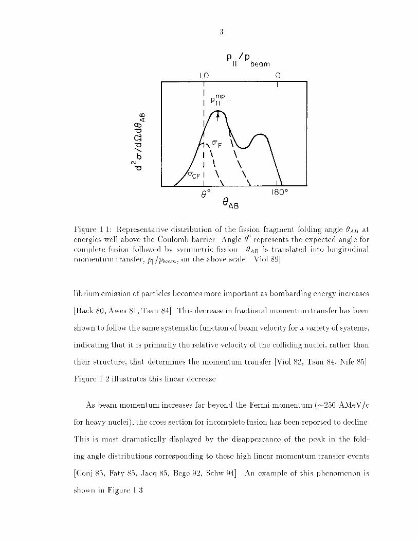
Figure 1.1 shows a typical �ssion fragment folding angle distribution with contri-
butions from complete fusion, incomplete fusion, and target �ssion. The complete
fusion component (�CF ) is peaked at an angle corresponding to complete momen-
tum transfer, whereas the inclusive component for central collisions (�F ), containing
incomplete and complete fusion, peaks at a slightly larger angle corresponding to in-
complete momentum transfer (pmp
k ). The low momentum transfer component is also
visible near 180o.
As beam energy is further increased from 10 AMeV up to � 50 AMeV, complete
fusion continues to become less probable, and more of the fusion-like cross section is
dominated by massive transfer processes. In the 14N + 238U system, for example, the
maximum estimated cross section for complete fusion has been measured to decrease
from 56% to 21% of the total �ssion cross section as beam energy increases from 15 to
30 AMeV [Tsan 84]. Correspondingly, the most probable momentum transfer, as a
fraction of beam momentum for fusion-like events decreases, indicating that preequi-
3
Figure 1.1: Representative distribution of the �ssion fragment folding angle �AB at
energies well above the Coulomb barrier. Angle �orepresents the expected angle for
complete fusion followed by symmetric �ssion. �AB is translated into longitudinalmomentum transfer, pk=pbeam, on the above scale. [Viol 89]
librium emission of particles becomes more important as bombarding energy increases
[Back 80, Awes 81, Tsan 84]. This decrease in fractional momentumtransfer has been
shown to follow the same systematic function of beam velocity for a variety of systems,
indicating that it is primarily the relative velocity of the colliding nuclei, rather than
their structure, that determines the momentum transfer [Viol 82, Tsan 84, Nife 85].
Figure 1.2 illustrates this linear decrease.
As beam momentum increases far beyond the Fermi momentum (�250 AMeV/c
for heavy nuclei), the cross section for incomplete fusion has been reported to decline.
This is most dramatically displayed by the disappearance of the peak in the fold-
ing angle distributions corresponding to these high linear momentum transfer events
[Conj 85, Faty 85, Jacq 85, Bege 92, Schw 94]. An example of this phenomenon is
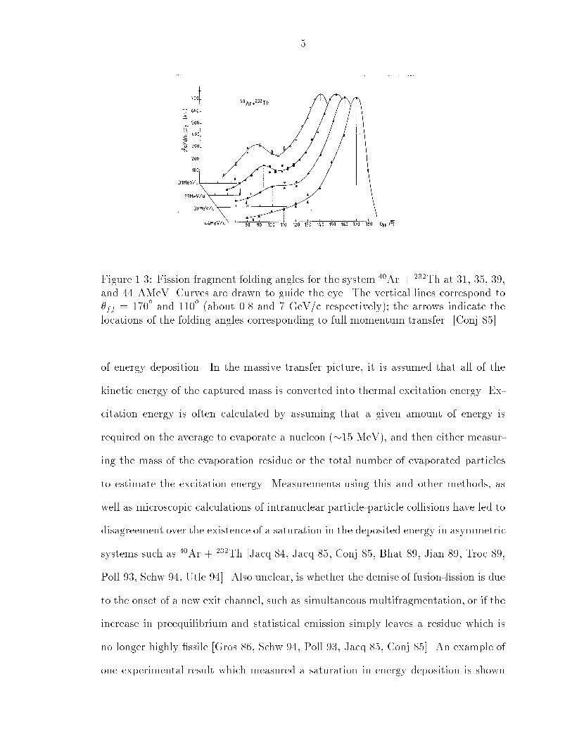
shown in Figure 1.3.
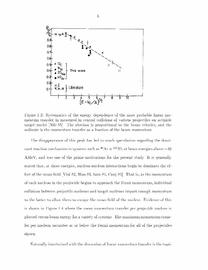
4
Figure 1.2: Systematics of the energy dependence of the most probable linear mo-mentum transfer in measured in central collisions of various projectiles on actinidetarget nuclei [Nife 85]. The abscissa is proportional to the beam velocity, and the
ordinate is the momentum transfer as a fraction of the beam momentum.
The disappearance of this peak has led to much speculation regarding the domi-
nant reaction mechanism in systems such as 40Ar + 232Th at beam energies above �40AMeV, and was one of the prime motivations for the present study. It is generally
stated that, at these energies, nucleon-nucleon interactions begin to dominate the ef-
fect of the mean �eld [Viol 82, Woo 83, Sain 84, Conj 85]. That is, as the momentum
of each nucleon in the projectile begins to approach the Fermi momentum, individual
collisions between projectile nucleons and target nucleons impart enough momentum
to the latter to allow them to escape the mean �eld of the nucleus. Evidence of this
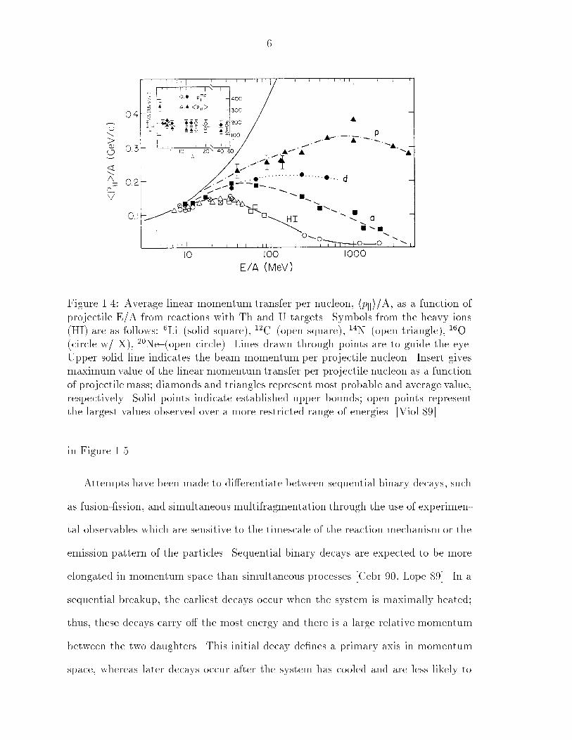
is shown in Figure 1.4 where the mean momentum transfer per projectile nucleon is
plotted versus beam energy for a variety of systems. The maximummomentum trans-
fer per nucleon saturates at or below the Fermi momentum for all of the projectiles
shown.
Naturally intertwined with the discussion of linear momentum transfer is the topic
5
Figure 1.3: Fission fragment folding angles for the system 40Ar + 232Th at 31, 35, 39,and 44 AMeV. Curves are drawn to guide the eye. The vertical lines correspond to�ff = 170
oand 110
o(about 0.8 and 7 GeV/c respectively); the arrows indicate the
locations of the folding angles corresponding to full momentum transfer. [Conj 85]
of energy deposition. In the massive transfer picture, it is assumed that all of the
kinetic energy of the captured mass is converted into thermal excitation energy. Ex-
citation energy is often calculated by assuming that a given amount of energy is
required on the average to evaporate a nucleon (�15 MeV), and then either measur-
ing the mass of the evaporation residue or the total number of evaporated particles
to estimate the excitation energy. Measurements using this and other methods, as
well as microscopic calculations of intranuclear particle-particle collisions have led to
disagreement over the existence of a saturation in the deposited energy in asymmetric
systems such as 40Ar + 232Th [Jacq 84, Jacq 85, Conj 85, Bhat 89, Jian 89, Troc 89,
Poll 93, Schw 94, Utle 94]. Also unclear, is whether the demise of fusion-�ssion is due
to the onset of a new exit channel, such as simultaneous multifragmentation, or if the
increase in preequilibrium and statistical emission simply leaves a residue which is
no longer highly �ssile [Gros 86, Schw 94, Poll 93, Jacq 85, Conj 85]. An example of
one experimental result which measured a saturation in energy deposition is shown
6
Figure 1.4: Average linear momentum transfer per nucleon, hpki/A, as a function of
projectile E/A from reactions with Th and U targets. Symbols from the heavy ions(HI) are as follows: 6Li{(solid square), 12C{(open square), 14N{(open triangle), 16O{(circle w/ X), 20Ne{(open circle). Lines drawn through points are to guide the eye.Upper solid line indicates the beam momentum per projectile nucleon. Insert givesmaximum value of the linear momentum transfer per projectile nucleon as a function
of projectile mass; diamonds and triangles represent most probable and average value,respectively. Solid points indicate established upper bounds; open points representthe largest values observed over a more restricted range of energies. [Viol 89]
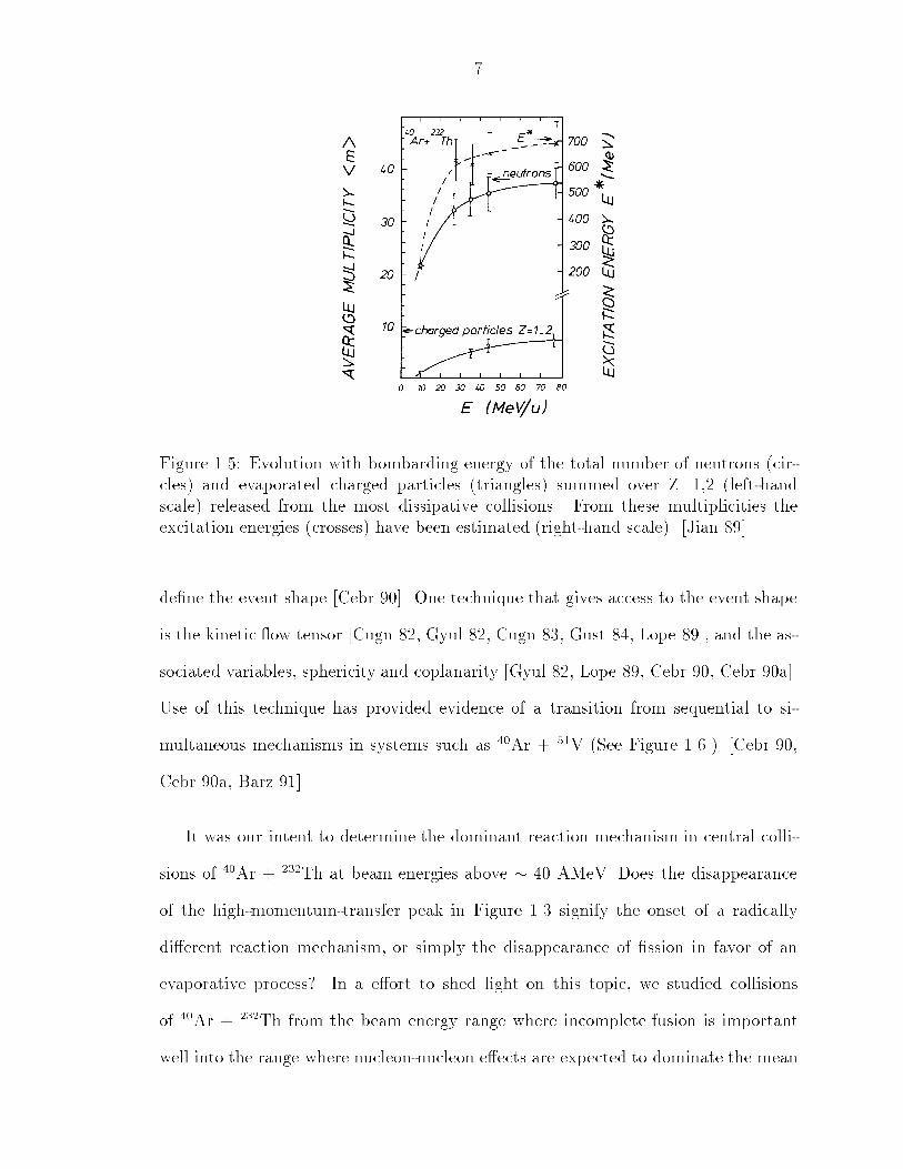
in Figure 1.5.
Attempts have been made to di�erentiate between sequential binary decays, such
as fusion-�ssion, and simultaneous multifragmentation through the use of experimen-
tal observables which are sensitive to the timescale of the reaction mechanism or the
emission pattern of the particles. Sequential binary decays are expected to be more
elongated in momentum space than simultaneous processes [Cebr 90, Lope 89]. In a
sequential breakup, the earliest decays occur when the system is maximally heated;
thus, these decays carry o� the most energy and there is a large relative momentum
between the two daughters. This initial decay de�nes a primary axis in momentum
space, whereas later decays occur after the system has cooled and are less likely to
7
Figure 1.5: Evolution with bombarding energy of the total number of neutrons (cir-cles) and evaporated charged particles (triangles) summed over Z=1,2 (left-handscale) released from the most dissipative collisions. From these multiplicities theexcitation energies (crosses) have been estimated (right-hand scale). [Jian 89]
de�ne the event shape [Cebr 90]. One technique that gives access to the event shape
is the kinetic ow tensor [Cugn 82, Gyul 82, Cugn 83, Gust 84, Lope 89], and the as-
sociated variables, sphericity and coplanarity [Gyul 82, Lope 89, Cebr 90, Cebr 90a].
Use of this technique has provided evidence of a transition from sequential to si-
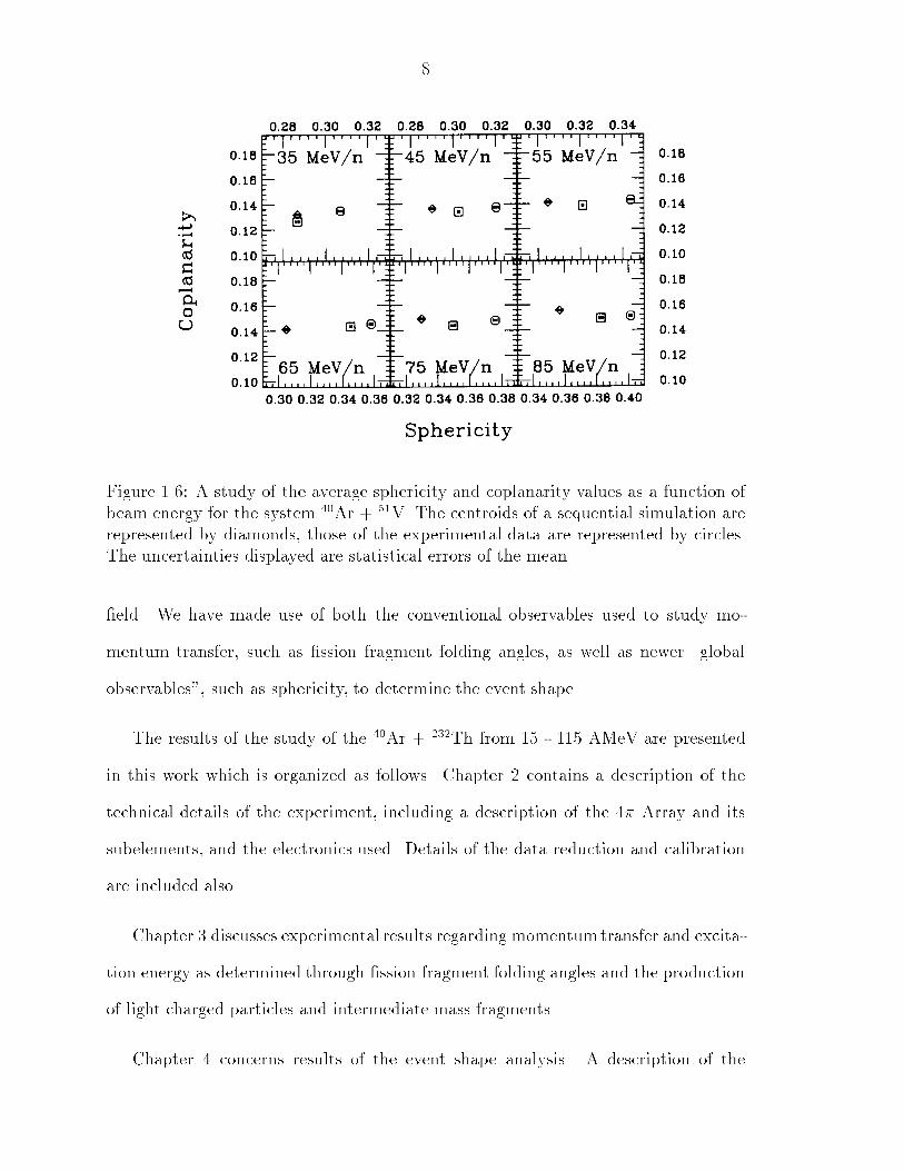
multaneous mechanisms in systems such as 40Ar + 51V (See Figure 1.6.) [Cebr 90,
Cebr 90a, Barz 91].
It was our intent to determine the dominant reaction mechanism in central colli-
sions of 40Ar + 232Th at beam energies above � 40 AMeV. Does the disappearance
of the high-momentum-transfer peak in Figure 1.3 signify the onset of a radically
di�erent reaction mechanism, or simply the disappearance of �ssion in favor of an
evaporative process? In a e�ort to shed light on this topic, we studied collisions
of 40Ar + 232Th from the beam energy range where incomplete fusion is important
well into the range where nucleon-nucleon e�ects are expected to dominate the mean
8
Figure 1.6: A study of the average sphericity and coplanarity values as a function of
beam energy for the system 40Ar + 51V. The centroids of a sequential simulation are
represented by diamonds, those of the experimental data are represented by circles.The uncertainties displayed are statistical errors of the mean.
�eld. We have made use of both the conventional observables used to study mo-
mentum transfer, such as �ssion fragment folding angles, as well as newer \global
observables", such as sphericity, to determine the event shape.
The results of the study of the 40Ar + 232Th from 15 - 115 AMeV are presented
in this work which is organized as follows. Chapter 2 contains a description of the
technical details of the experiment, including a description of the 4� Array and its
subelements, and the electronics used. Details of the data reduction and calibration
are included also.
Chapter 3 discusses experimental results regarding momentumtransfer and excita-
tion energy as determined through �ssion fragment folding angles and the production
of light charged particles and intermediate mass fragments.
Chapter 4 concerns results of the event shape analysis. A description of the
9
method for determining the event shape is presented, along with details regarding
various e�ects which must be considered in the analysis.
Chapter 5 contains a summary and brief conclusions. Appendix A discusses the
experimental determination of the centrality of an event, and the technique of impact
parameter selection based on global observables is explained. Also discussed are
the concept of autocorrelations and the reasoning behind the choices of the global
observables used.

10
Chapter 2
Experimental Details
2.1 Introduction
The experiment was performed at the National Superconducting Cyclotron Labora-
tory (NSCL) at Michigan State University (MSU) where 40Ar beams of E = 15 to
115 AMeV accelerated by the K1200 cyclotron bombarded a 1 mg/cm2 232Th tar-
get. Reaction products of nuclear collisions were detected with the MSU 4� Array
[West 85]. Event information from each collision was digitized on an event-by-event
basis, written to magnetic tape, and analyzed o�-line.
The 4� Array, as out�tted for this experiment, provided nearly 4� detection of
light charged particles, intermediate mass fragments, and �ssion fragments. Most
previous experiments studying this system did not have coverage as comprehensive
as that provided by the Array, either in geometric acceptance or range of particle
types identi�ed. It was our hope that with the extensive coverage of this system over
such a wide range of beam energies we could determine the evolution of the reaction
mechanism in central collisions. The following sections in this chapter describe in
detail the 4� Array, its various components and their acceptance, and the methods
used to calibrate them.
11

12
2.2 Michigan State University 4� Array
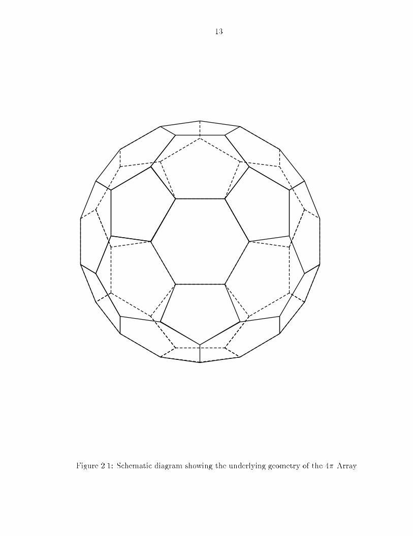
Figure 2.1 depicts the underlying geometry of the MSU 4� Array. The 4� Array
consists of 30 separate sub-modules enclosed within a 32-faced, aluminum, truncated
icosahedron. Externally, it resembles a soccer ball, having 20 hexagonal faces, and
12 pentagonal ones. All of the hexagonal faces, and 10 of the pentagonal ones serve
as backplates upon which the 30 modules are mounted. The remaining pentagonal
faces serve as an entrance and exit for the incident beam.
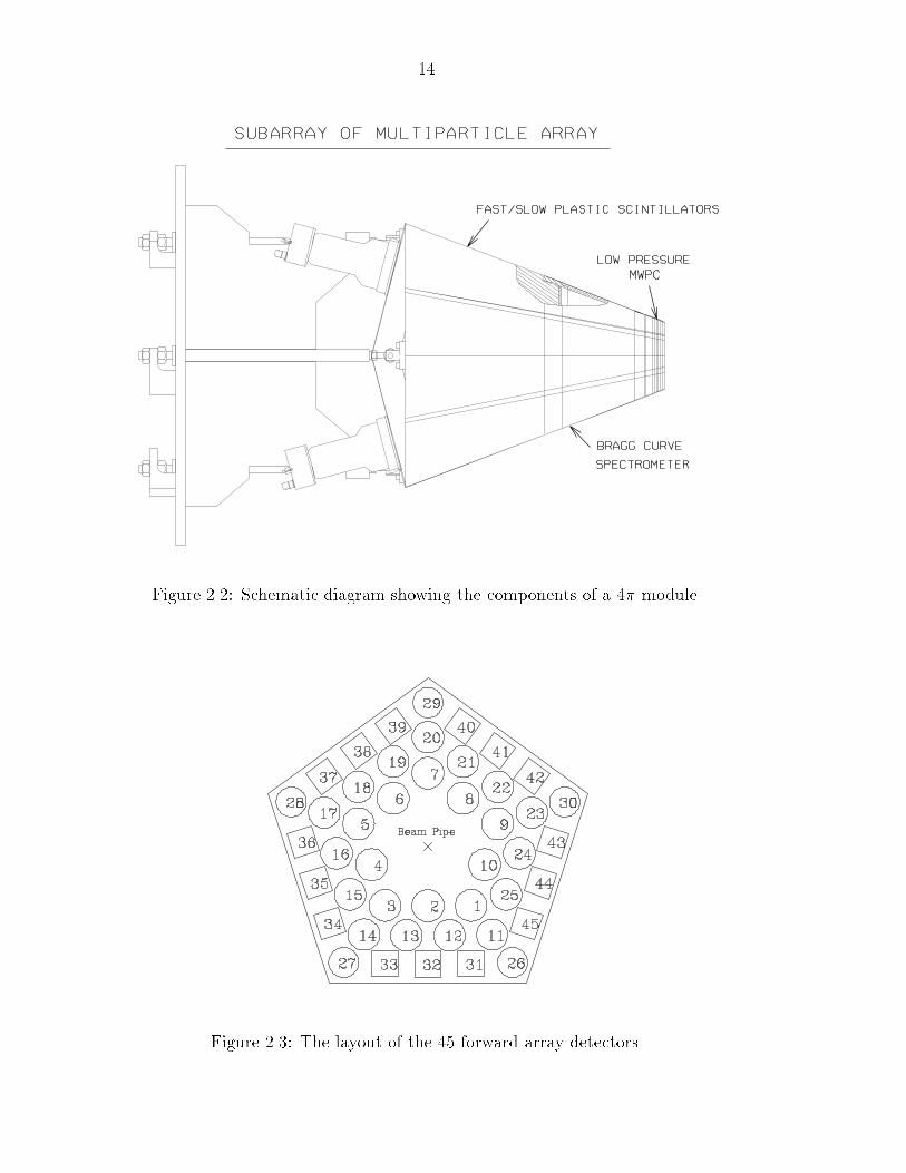
Figure 2.2 shows a diagram of a hexagonal module of the 4� Array. Each hexag-
onal(pentagonal) module consists of 6(5) close packed plastic phoswich detectors.
Mounted in front of each phoswich is a gas chamber which can be used as a �E
detector for particles stopping in the thin layer of the phoswich detector, and as a
standalone Bragg Curve counter (BCC). The BCCs in the 5 most forward modules
are subdivided into 6 separate detectors. In front of each BCC is a low pressure
multi-wire proportional counter (MWPC) for the detection of slow, heavy fragments.
In total, these sub-modules making up the main ball consist of 170 phoswich detec-
tors, 55 BCCs, and 30 MWPCs, and cover lab polar angles from approximately 18oto
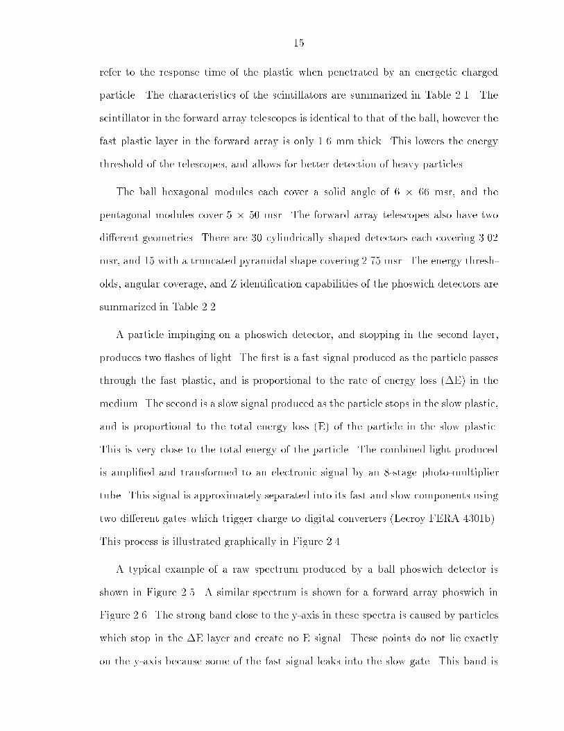
162o. In addition to the detectors in the main ball, the 4� Array also contains a
forward array consisting of 45 plastic phoswiches. These are not close packed, and
cover approximately 54% of the solid angle from 7oto 18
o. The layout of the forward
array is shown in Figure 2.3.
2.2.1 Plastic Phoswich Counters
The 170 ball plastic phoswiches are composed of 3 mm thick sheet of Bicron BC-412
fast plastic scintillator (�E component) optically coupled to 25 cm thick block of
Bicron BC-444 slow plastic scintillator (E component). The terms \fast" and \slow"
13
Figure 2.1: Schematic diagram showing the underlying geometry of the 4� Array.
14
Figure 2.2: Schematic diagram showing the components of a 4� module.
Figure 2.3: The layout of the 45 forward array detectors.
15
refer to the response time of the plastic when penetrated by an energetic charged
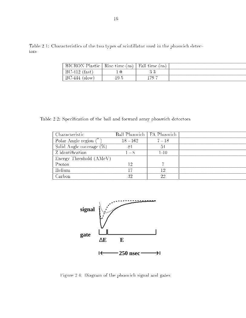
particle. The characteristics of the scintillators are summarized in Table 2.1. The
scintillator in the forward array telescopes is identical to that of the ball, however the
fast plastic layer in the forward array is only 1.6 mm thick. This lowers the energy
threshold of the telescopes, and allows for better detection of heavy particles.
The ball hexagonal modules each cover a solid angle of 6 � 66 msr, and the
pentagonal modules cover 5 � 50 msr. The forward array telescopes also have two
di�erent geometries. There are 30 cylindrically shaped detectors each covering 3.02
msr, and 15 with a truncated pyramidal shape covering 2.75 msr. The energy thresh-
olds, angular coverage, and Z identi�cation capabilities of the phoswich detectors are
summarized in Table 2.2.
A particle impinging on a phoswich detector, and stopping in the second layer,
produces two ashes of light. The �rst is a fast signal produced as the particle passes
through the fast plastic, and is proportional to the rate of energy loss (�E) in the
medium. The second is a slow signal produced as the particle stops in the slow plastic,
and is proportional to the total energy loss (E) of the particle in the slow plastic.
This is very close to the total energy of the particle. The combined light produced
is ampli�ed and transformed to an electronic signal by an 8-stage photo-multiplier
tube. This signal is approximately separated into its fast and slow components using
two di�erent gates which trigger charge to digital converters (Lecroy FERA 4301b).
This process is illustrated graphically in Figure 2.4.
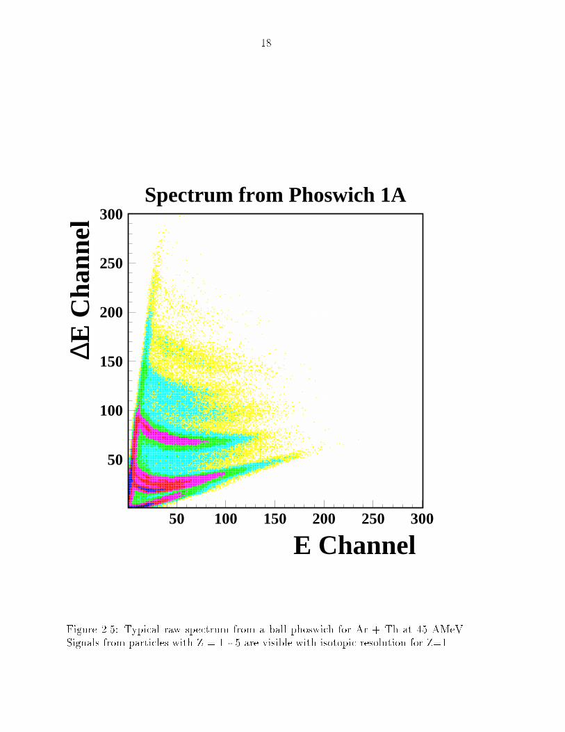
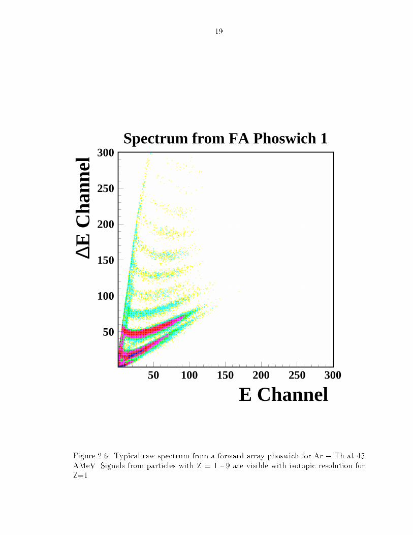
A typical example of a raw spectrum produced by a ball phoswich detector is
shown in Figure 2.5. A similar spectrum is shown for a forward array phoswich in
Figure 2.6. The strong band close to the y-axis in these spectra is caused by particles
which stop in the �E layer and create no E signal. These points do not lie exactly
on the y-axis because some of the fast signal leaks into the slow gate. This band is
16
Table 2.1: Characteristics of the two types of scintillator used in the phoswich detec-tors.
BICRON Plastic Rise time (ns) Fall time (ns)
BC-412 (fast) 1.0 3.3
BC-444 (slow) 19.5 179.7
Table 2.2: Speci�cation of the ball and forward array phoswich detectors.
Characteristic Ball Phoswich FA Phoswich
Polar Angle region (o) 18 - 162 7 - 18
Solid Angle coverage (%) 84 54
Z identi�cation 1 - 8 1-10
Energy Threshold (AMeV)Proton 12 7
Helium 17 12
Carbon 32 22
signal
gate∆E E
250 nsec
Figure 2.4: Diagram of the phoswich signal and gates.
17
known as the punch-in line. Similarly, the band near the x-axis is caused by particles
such as neutrons or gamma rays, which leave little or no signal in the �E layer but
leave a large signal in the E layer. This band is called the neutral line. Both of these
spectra are displayed in 512 channel resolution, but the data are recorded in 2048
channel resolution.
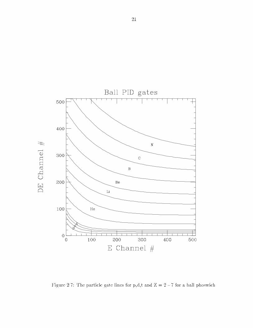
Phoswich Calibration
Because of the large number of detectors in the 4� Array, a system has been devised
to minimize the amount of time required to calibrate each detector. This process
involves creating a two-dimensional calibrated template to which all of the phoswich
spectra are then matched. There are two components to this template: the gate lines
and the response function.
The gate lines are created by drawing them directly onto a typical spectrum using
a mouse driven graphics program. Before this is done, the spectrum is transformed
such that the punch-in line and neutral line lie exactly on the x and y axes. This is
done using the following transformations [Cebr 90]:
CHf = (�Echannel � Y0)� (Echannel �X0)Mn
CHs = (Echannel �X0) � (�Echannel � Y0)=Mp; (2.1)
where �Echannel and Echannel are the fast and slow channel numbers recorded during
the experiment,Mn and Mp are the slopes of the neutral and punch-in lines, and X0
and Y0 are the coordinates of the crossing point of the neutral and punch-in lines,
representing the o�set of the ADCs. The quantitiesCHf and CHs are the transformed
channel numbers. The gatelines are used to produce a map �le which converts the
transformed channel numbers into the correct atomic number for each particle. As
isotopic resolution is possible only for Z=1, all other elements are assigned a mass
18
Spectrum from Phoswich 1A
E Channel
∆E C
hann
el
50
100
150
200
250
300
50 100 150 200 250 300
Figure 2.5: Typical raw spectrum from a ball phoswich for Ar + Th at 45 AMeV.
Signals from particles with Z = 1 - 5 are visible with isotopic resolution for Z=1.
19
Spectrum from FA Phoswich 1
E Channel
∆E C
hann
el
50
100
150
200
250
300
50 100 150 200 250 300
Figure 2.6: Typical raw spectrum from a forward array phoswich for Ar + Th at 45
AMeV. Signals from particles with Z = 1 - 9 are visible with isotopic resolution for
Z=1.
20
number corresponding to the most common isotope. Phoswich spectra from each
detector are then transformed and gain matched to �t these gate lines using another
program with a graphical interface, and the gain parameters are stored in a �le on
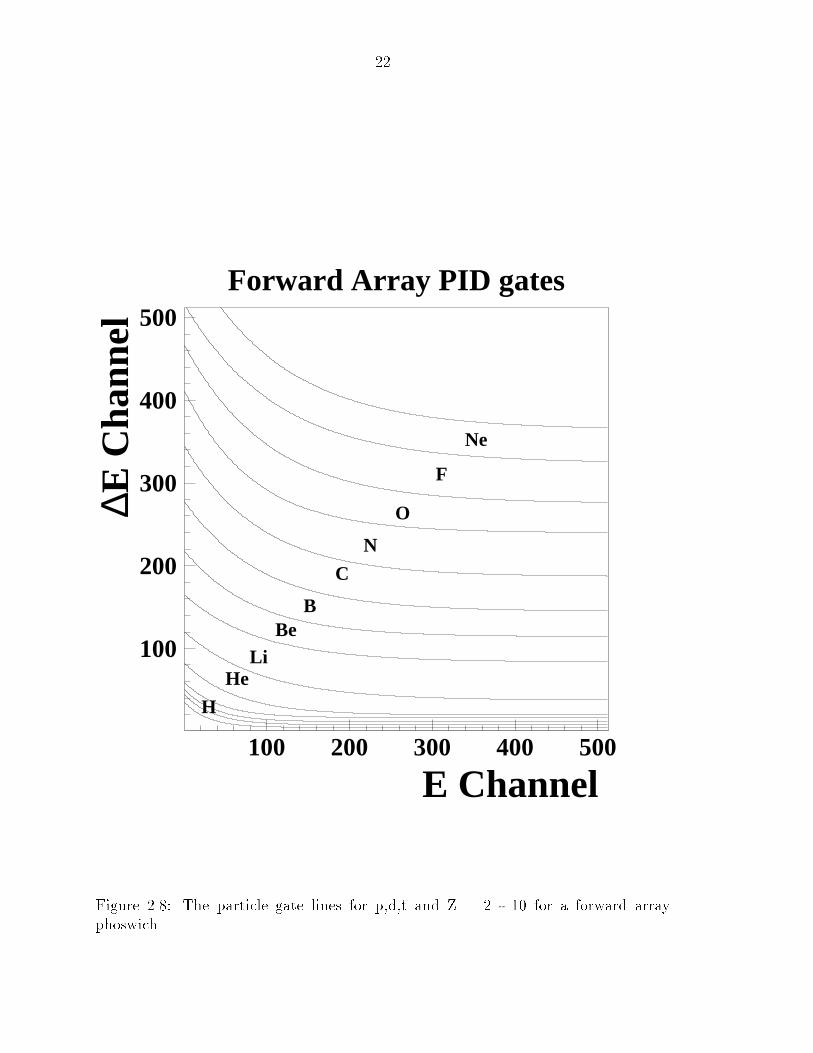
a hard disk. Figure 2.7 and Figure 2.8 show the gate lines for the ball and forward
array phoswiches used for these data.
The response functions used are determined from a previous calibration experi-
ment [Cebr 90], and have the form:
CHs = aE1:4s=A
0:4Z
0:8
CHf = bE0:5f� c: (2.2)
These equations convert the transformed fast and slow channel numbers into the
energy lost in the corresponding plastic. The arbitrary constants a,b, and c are de-
termined by �tting the lines following this functional form to the same representative
spectrum used to create the gate lines. Thus, when the spectra are �t to the gate line
template for particle identi�cation, a map is also obtained between the raw channel
number and the energy lost in the slow and fast plastic. The �nal response functions
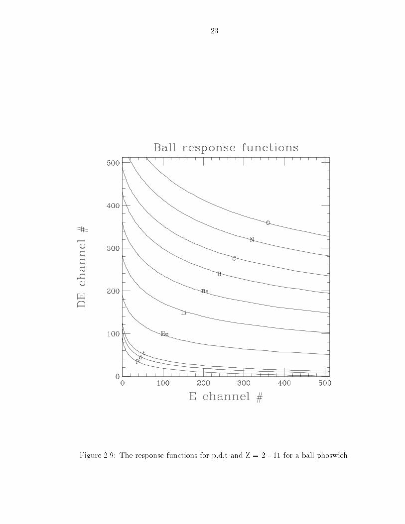
used for the ball are shown in Figure 2.9.
Thus far, we have described a process to convert the raw channel number associ-
ated with a detected particle into the correct atomic number and kinetic energy lost
in the fast and slow plastic. The �nal step is to determine an incident energy for the
particle based on its energy loss. This is done using the energy loss program DONNA.
By providing DONNA with the densities and thickness of the detector media we ob-
tained the �nal link which, in combination with the response functions, allowed us to
convert the raw channel number directly into incident kinetic energy.
To summarize, a template is produced for the ball and forward array which all
phoswich spectra are matched to. From this template look-up tables are made which
21
Figure 2.7: The particle gate lines for p,d,t and Z = 2 - 7 for a ball phoswich.
22
Forward Array PID gates
E Channel
∆E C
hann
el
H
HeLi
BeB
C
N
O
F
Ne
100
200
300
400
500
100 200 300 400 500
Figure 2.8: The particle gate lines for p,d,t and Z = 2 - 10 for a forward array
phoswich.
23
Figure 2.9: The response functions for p,d,t and Z = 2 - 11 for a ball phoswich.
24
map raw channel number into particle type and incident energy. Angles of the de-
tected particles are assigned as the geometric mean angle of the corresponding detec-
tor. Using these tables, the raw data tapes are �ltered onto \physics" tapes which
contain information regarding the Z,A,�,�, and kinetic energy of each particle de-
tected.
2.2.2 Bragg Curve Counters
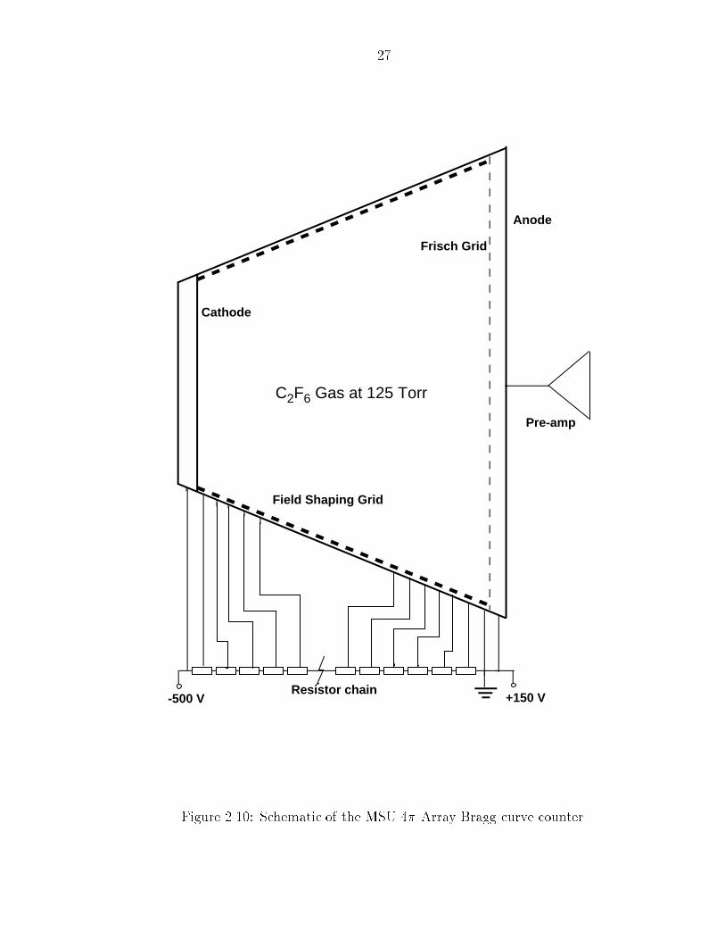
The 4� Array contains 55 Bragg Curve spectrometers (BCC) which are gas-�lled ion-
ization chambers. The chambers each consist of a hexagonal or pentagonal pyramidal
housing of G10 �berglass which is mounted directly on the face of the phoswich mod-
ule. (See Figure 2.10.) A 2.5 �m thick aluminum coating is evaporated on the face
of the phoswich fast plastic, and this serves as the anode for the BCC. In the �rst
ring (closest to the beam axis) of �ve hexagonal modules, the anode is separated into
6 electrically isolated segments corresponding to the 6 fast plastic segments. Thus
there are e�ectively 55 BCCs in the 4� Array, even though there are only 30 separate
gas volumes. The front pressure windows of the BCCs are made of 900 �g/cm2 thick,
aluminized kapton. The windows are epoxied to a stainless steel frame and serve as
the cathodes for the BCCs. The distance between the cathode and the anode is 13.36
cm.
A Frisch grid is installed in the BCCs parallel to and 1 cm above the anode. The
Frisch grid is made of 12.5�m gold plated tungsten wires spaced .5 mm apart, and
epoxied with conductive epoxy to a copper strip on the BCC frame. The grid is held
at ground potential and serves to shield the anode from the induced image charge
caused by the drifting electrons. An approximately radial �eld within the chamber
is produced by using a �eld shaping grid which lines the inside of the housing. The
grid consists of 21 copper strips, each encircling the the volume of the chamber and
25
spaced between the Frisch grid and the cathode. The strips are linked by 21 1.55 M
resistors creating a 21 stage voltage drop between the negative cathode potential and
ground.
Charged particles (positive ions) entering the chamber ionize the gas within, and
lose energy as they travel. If one plots the rate of this energy loss against the distance
of penetration, the functional form is called a Bragg curve. The Bragg curve typically
peaks close to the end of the ight path of the particle since the rate of energy loss is
greatest when the particle is moving very slowly and spending more time in the �eld
of each particle it encounters. At the very end of ight path, the charge of the ion
is reduced due to electron pickup and the energy loss curve decreases quickly. The
energy loss falls to zero when the ion becomes a neutral atom.
The electron-ion pairs created by the impinging particle drift along the radial �eld
lines to the cathode and anode. The negative signal produced on the anode is fed into
a charge-sensitive preampli�er and integrated. This signal is in turn fed into a shaping
ampli�er with both a fast and slow time constant. The fast channel di�erentiates the
input signal to obtain the shape of the original signal before integration. A small
amount of integration is used to suppress noise. This results in a Bragg curve signal
with peak height proportional to the charge of the particle which created it. The slow
channel shapes the integrated signal with two stages of di�erentiation and integration
producing a signal whose peak is proportional to the energy of the incident particle.
Each of these signals is fed into a separate peak sensing ADC (Silena 4418/v), digitized
and written to magnetic tape.
This method of identi�cation will not work if the particle does not stop in the
gas volume because the peak of the Bragg curve will not occur in the detector. In
that case, the particles that punch through and stop in the fast plastic behind the
BCC are identi�ed by the �E signal left in the BCC and the E signal left in the
26
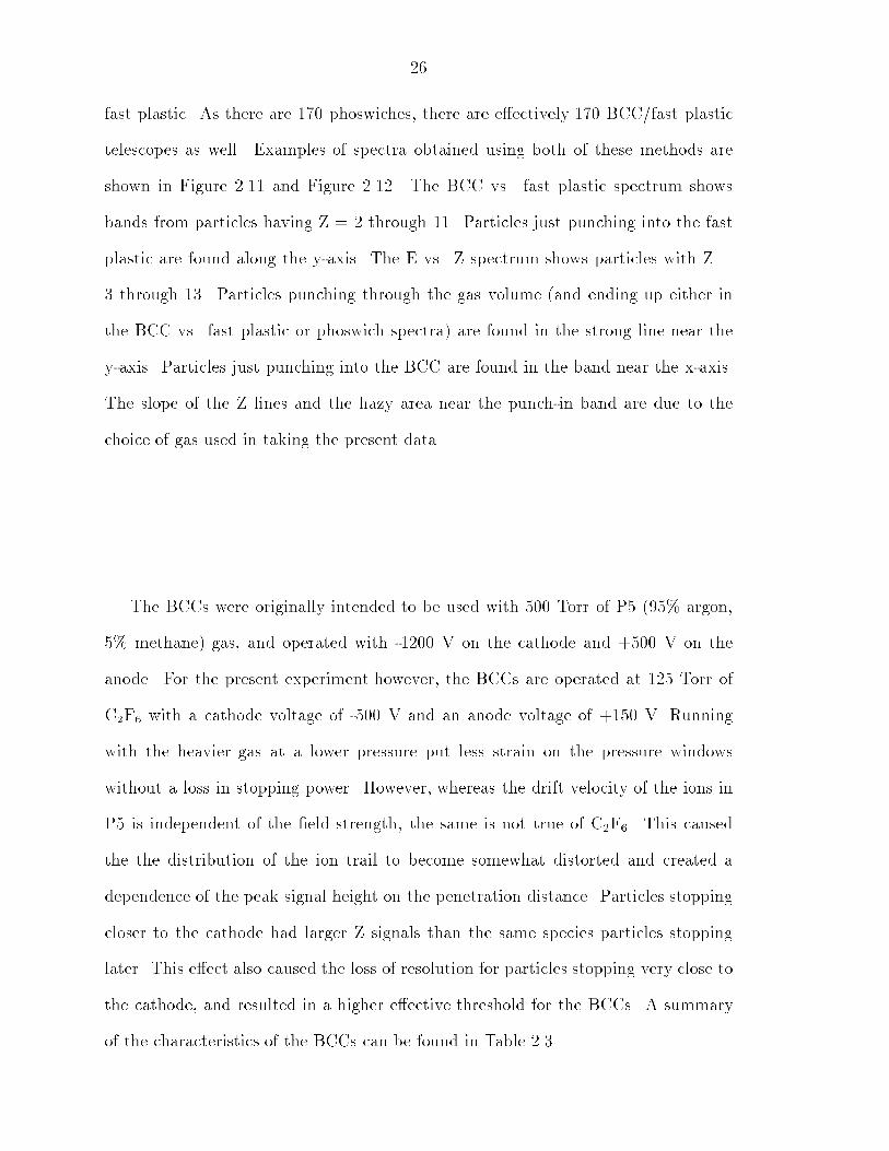
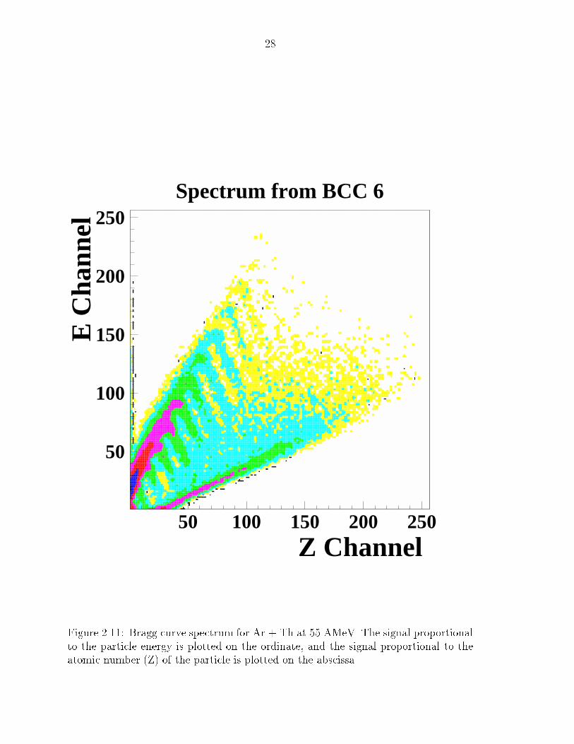
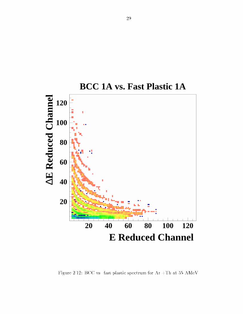
fast plastic. As there are 170 phoswiches, there are e�ectively 170 BCC/fast plastic
telescopes as well. Examples of spectra obtained using both of these methods are
shown in Figure 2.11 and Figure 2.12. The BCC vs. fast plastic spectrum shows
bands from particles having Z = 2 through 11. Particles just punching into the fast
plastic are found along the y-axis. The E vs. Z spectrum shows particles with Z =
3 through 13. Particles punching through the gas volume (and ending up either in
the BCC vs. fast plastic or phoswich spectra) are found in the strong line near the
y-axis. Particles just punching into the BCC are found in the band near the x-axis.
The slope of the Z lines and the hazy area near the punch-in band are due to the
choice of gas used in taking the present data.
The BCCs were originally intended to be used with 500 Torr of P5 (95% argon,
5% methane) gas, and operated with -1200 V on the cathode and +500 V on the
anode. For the present experiment however, the BCCs are operated at 125 Torr of
C2F6 with a cathode voltage of -500 V and an anode voltage of +150 V. Running
with the heavier gas at a lower pressure put less strain on the pressure windows
without a loss in stopping power. However, whereas the drift velocity of the ions in
P5 is independent of the �eld strength, the same is not true of C2F6. This caused
the the distribution of the ion trail to become somewhat distorted and created a
dependence of the peak signal height on the penetration distance. Particles stopping
closer to the cathode had larger Z signals than the same species particles stopping
later. This e�ect also caused the loss of resolution for particles stopping very close to
the cathode, and resulted in a higher e�ective threshold for the BCCs. A summary
of the characteristics of the BCCs can be found in Table 2.3.
27
C2F6 Gas at 125 Torr
Field Shaping Grid
Frisch Grid
Anode
Cathode
-500 V +150 VResistor chain
Pre-amp
Figure 2.10: Schematic of the MSU 4� Array Bragg curve counter.
28
Spectrum from BCC 6
Z Channel
E C
hann
el
50
100
150
200
250
50 100 150 200 250
Figure 2.11: Bragg curve spectrum for Ar + Th at 55 AMeV. The signal proportional
to the particle energy is plotted on the ordinate, and the signal proportional to theatomic number (Z) of the particle is plotted on the abscissa.
29
BCC 1A vs. Fast Plastic 1A
E Reduced Channel
∆E R
educ
ed C
hann
el
20
40
60
80
100
120
20 40 60 80 100 120
Figure 2.12: BCC vs. fast plastic spectrum for Ar +Th at 55 AMeV.
30
Table 2.3: Speci�cations of the Bragg curve counters.
Characteristic BCC vs. FP BCC E vs. Z
Polar Angle region (o) 18 - 162 18 -162
Solid Angle coverage (%) 84 84
Z identi�cation 2 - 18 3 - 18
Energy Threshold (AMeV)
Lithium 4.0 2.0
Boron 5.0 3.0
Carbon 5.5 4.0
BCC Calibration
The calibration of the Bragg curve vs. fast plastic (�E/E) spectra is accomplished in
a fashion similar to the phoswich calibration. The di�erence lies in that the gate lines
as well as the response functions are generated from a known functional form, whereas
with the phoswiches the gate lines are drawn in by hand. The response function for
the fast plastic has the same form as that used for the slow plastic in the phoswich
calibration, since in this case the fast plastic is the stopping detector. The form is
CHf = �E1:4f=(A0:4
Z0:8): (2:3)
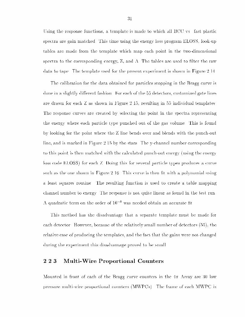
A response curve for the BCC was originally determined to be linear:
CHBCC = �EBCC (2:4)
during a �eld test using a BCC with P5 gas and corresponding speci�cations listed
above [Cebr 91] (See Figure 2.13). In that test run, it was determined that the BCC
energy response was independent of particle type. However, in the present experiment,
it is necessary to introduce a charge dependence into the energy calibration as an
exponent in the energy term.
CHBCC = �EC(Z)BCC
(2:5)
31
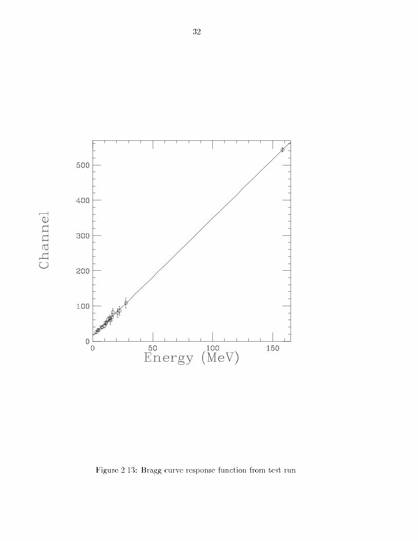
Using the response functions, a template is made to which all BCC vs. fast plastic
spectra are gain matched. This time using the energy loss program ELOSS, look-up
tables are made from the template which map each point in the two-dimensional
spectra to the corresponding energy, Z, and A. The tables are used to �lter the raw
data to tape. The template used for the present experiment is shown in Figure 2.14.
The calibration for the data obtained for particles stopping in the Bragg curve is
done in a slightly di�erent fashion. For each of the 55 detectors, customized gate lines
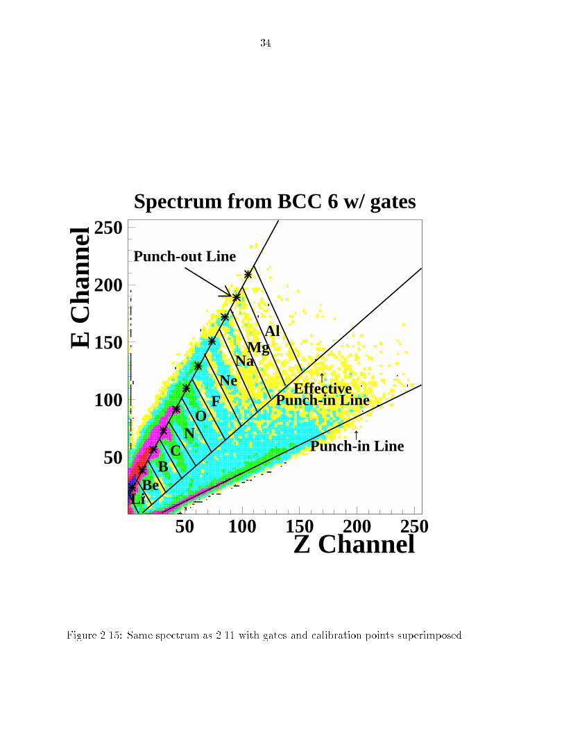
are drawn for each Z as shown in Figure 2.15, resulting in 55 individual templates.
The response curves are created by selecting the point in the spectra representing
the energy where each particle type punched out of the gas volume. This is found
by looking for the point where the Z line bends over and blends with the punch-out
line, and is marked in Figure 2.15 by the stars. The y-channel number corresponding
to this point is then matched with the calculated punch-out energy (using the energy
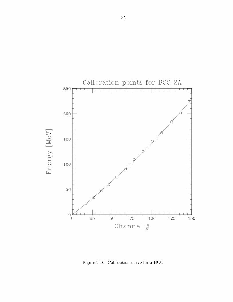
loss code ELOSS) for each Z. Doing this for several particle types produces a curve
such as the one shown in Figure 2.16. This curve is then �t with a polynomial using
a least squares routine. The resulting function is used to create a table mapping
channel number to energy. The response is not quite linear as found in the test run.
A quadratic term on the order of 10�3 was needed obtain an accurate �t.
This method has the disadvantage that a separate template must be made for
each detector. However, because of the relatively small number of detectors (55), the
relative ease of producing the templates, and the fact that the gains were not changed
during the experiment this disadvantage proved to be small.
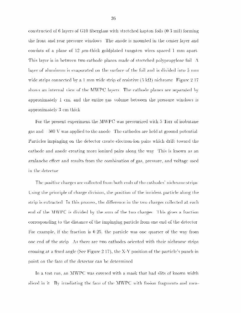
2.2.3 Multi-Wire Proportional Counters
Mounted in front of each of the Bragg curve counters in the 4� Array are 30 low
pressure multi-wire proportional counters (MWPCs). The frame of each MWPC is
32
Figure 2.13: Bragg curve response function from test run.
33
BCC v. Fast Plastic PID gates
E Channel
∆E C
hann
el
HeLi
BeB
CN
OF
NeNa
MgAl
SiP
S
Cl
Ar
100
200
300
400
500
100 200 300 400 500
Figure 2.14: Template for a BCC vs. Fast Plastic spectrum.
34
Spectrum from BCC 6 w/ gates
50
100
150
200
250
50 100 150 200 250Z Channel
E C
hann
el
Punch-in Line
EffectivePunch-in Line
Punch-out Line
↑
↑
LiBe
BC
NO
FNe
NaMg
Al
Figure 2.15: Same spectrum as 2.11 with gates and calibration points superimposed.
35
Figure 2.16: Calibration curve for a BCC.
36
constructed of 6 layers of G10 �berglass with stretched kapton foils (0.3 mil) forming
the front and rear pressure windows. The anode is mounted in the center layer and
consists of a plane of 12 �m-thick goldplated tungsten wires spaced 1 mm apart.
This layer is in between two cathode planes made of stretched polypropylene foil. A
layer of aluminum is evaporated on the surface of the foil and is divided into 5 mm
wide strips connected by a 1 mm wide strip of resistive (5 k) nichrome. Figure 2.17
shows an internal view of the MWPC layers. The cathode planes are separated by
approximately 1 cm, and the entire gas volume between the pressure windows is
approximately 3 cm thick.
For the present experiment the MWPC was pressurized with 5 Torr of isobutane
gas and +500 V was applied to the anode. The cathodes are held at ground potential.
Particles impinging on the detector create electron-ion pairs which drift toward the
cathode and anode creating more ionized pairs along the way. This is known as an
avalanche e�ect and results from the combination of gas, pressure, and voltage used
in the detector.
The positive charges are collected from both ends of the cathodes' nichrome strips.
Using the principle of charge division, the position of the incident particle along the
strip is extracted. In this process, the di�erence in the two charges collected at each
end of the MWPC is divided by the sum of the two charges. This gives a fraction
corresponding to the distance of the impinging particle from one end of the detector.
For example, if the fraction is 0.25, the particle was one quarter of the way from
one end of the strip. As there are two cathodes oriented with their nichrome strips
crossing at a �xed angle (See Figure 2.17), the X-Y position of the particle's punch-in
point on the face of the detector can be determined.
In a test run, an MWPC was covered with a mask that had slits of known width
sliced in it. By irradiating the face of the MWPC with �ssion fragments and mea-
37
suring the resulting position spectrum, we were able to determine that the MWPCs
have an angular resolution of 1o.
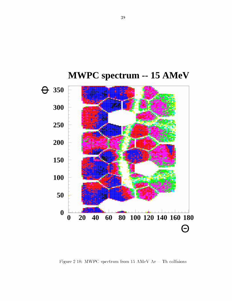
A position spectrum of particles produced in 15 AMeV Ar + Th collisions and
measured in the MWPCs is shown in Figure 2.18. In the �gure, the polar and
azimuthal angular positions of the detected particles are unfolded and displayed.
Most of the MWPCs were working when this spectrum was recorded; dead detectors
are identi�able as white regions. Shadowing due to the target frame can be seen in
the region near 90o(lab).
The MWPCs were designed to detect �ssion fragments. Due to the low pressure
and small volume of gas used, they are not as e�cient for very light, fast particles.
However, IMFs can leave signi�cant signals in the MWPCs and must be separated
from the �ssion fragments. This is done by using the BCC behind the MWPC as a
veto detector. Particles leaving a signal in the MWPC and punching into the BCC
are designated as not being �ssion fragments.

38
Y
x
QL
QR
(QL QR- )/ (QL + QR)
L
X = L*
Figure 2.17: Exploded view of the MWPC. The X in the equation is the position ofthe particle along the x-axis. QL and QR are the charge collected on the left and
right ends of the cathode, respectively.
39
MWPC spectrum -- 15 AMeV
Θ
Φ
0
50
100
150
200
250
300
350
0 20 40 60 80 100 120 140 160 180
Figure 2.18: MWPC spectrum from 15 AMeV Ar + Th collisions

40
Chapter 3
Momentum Transfer and
Deposited Energy
3.1 Introduction
In this chapter we discuss the evolution of the momentum transfer and energy deposi-
tion in 40Ar + 232Th collisions as beam energy is increased from 15 to 115 AMeV. We
will study these topics via inclusive and exclusive measurements of �ssion fragment
folding angles, �ssion fragment azimuthal angles, and charged particle production.
3.2 Folding Angle Distributions
In investigating heavy �ssionable systems, a great deal can be learned from studying
the �ssion fragment folding angle distributions. The folding angle is simply the angle
between the two vectors de�ning the trajectory of each �ssion fragment in the lab
frame. In the frame of the �ssioning nucleus, these vectors would be approximately
180oapart as required by momentum conservation. However, when the fragments are
boosted into the lab frame, the folding angle is reduced by an amount directly related
to the velocity of the moving source [Back 80, Viol 82, Viol 89]. This is illustrated
graphically in Figure 3.1.
41
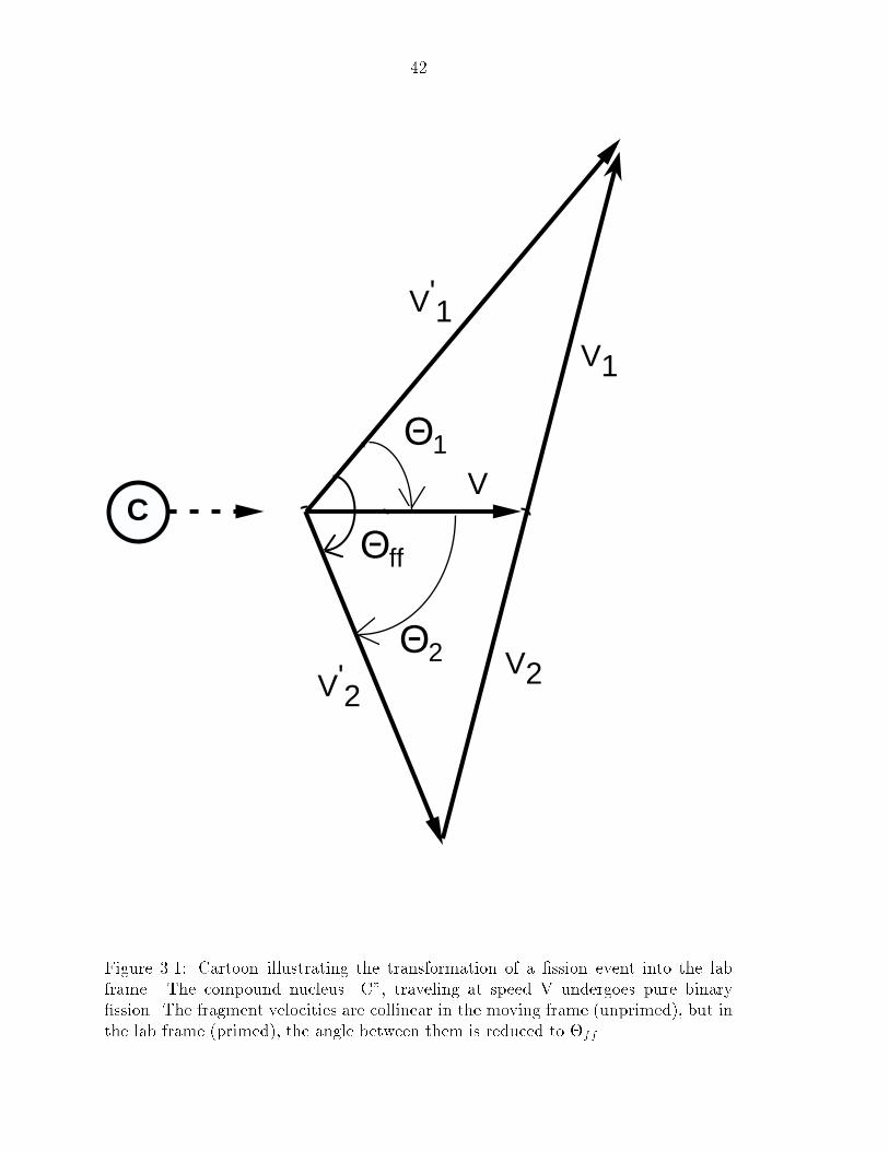
42
CΘff
V1
V2V'2
V'1
V
Θ2
Θ1
Figure 3.1: Cartoon illustrating the transformation of a �ssion event into the lab
frame. The compound nucleus \C", traveling at speed V undergoes pure binary
�ssion. The fragment velocities are collinear in the moving frame (unprimed), but inthe lab frame (primed), the angle between them is reduced to �ff .
43
The folding angle is usually de�ned as the sum of the polar angles of the two
�ssion fragments in the lab frame [Viol 82, Tsan 84, Viol 89]. That is
�ff = �1 +�2; (3:1)
where �1 and �2 are measured with respect to the beam axis. This de�nition is
adequate if the �ssion fragments are emitted close to a common plane with the beam
axis. However, as will be shown below, this is often not the case at high bombarding
energies. Because of the ability of the 4� Array to detect �ssion fragments in almost
all possible planes, we need a more general de�nition of opening angle. For this reason
we use
�ff = cos�1(f1.f2); (3:2)
where f1 and f2 are the unit vectors of the lab trajectories of the �ssion fragments,
assuming an emission from the center of the lab coordinate system.
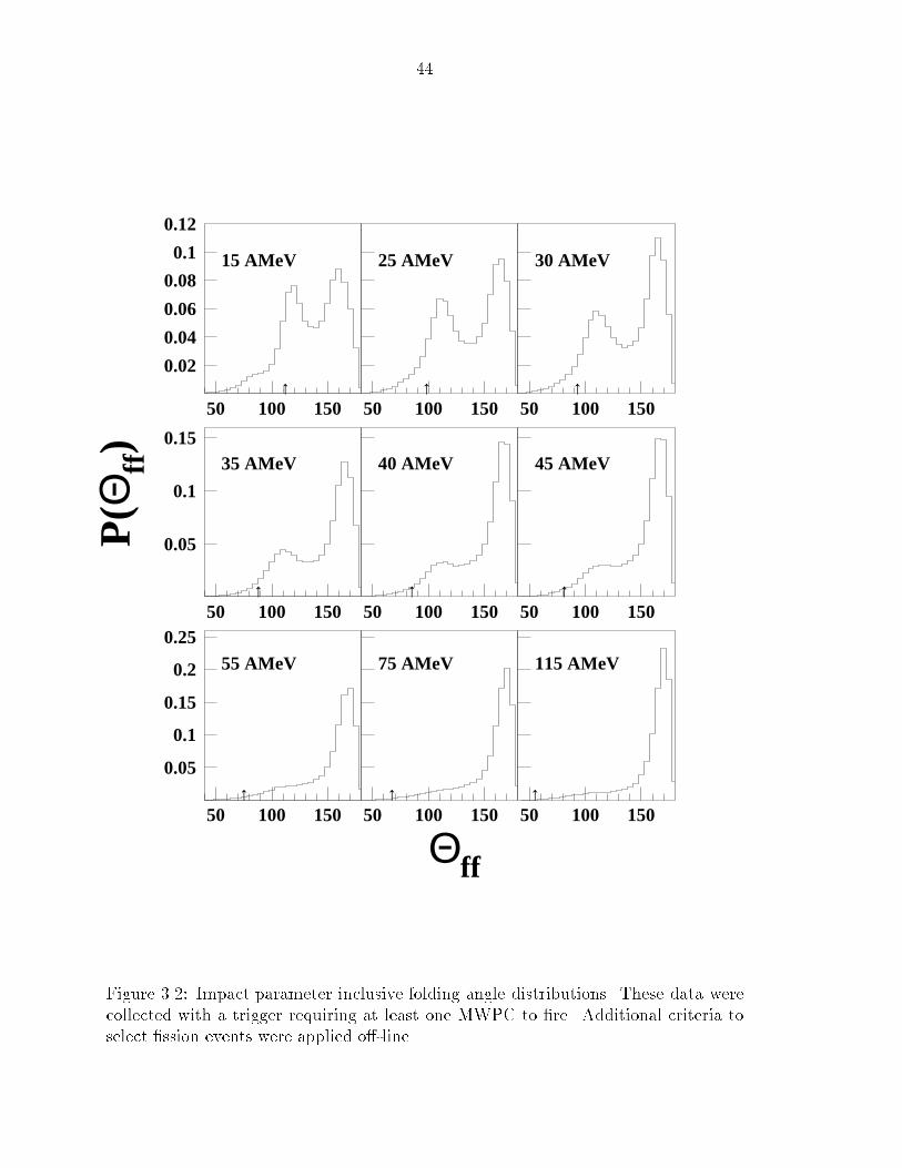
Figure 3.2 shows the inclusive distributions of �ssion fragment folding angles for
the 40Ar + 232Th system at all nine energies studied. These data were taken with a
trigger (called MWPC 1) requiring one MWPC to �re. There are two main charac-
teristics in each of these distributions resulting from di�erent interactions that can
be loosely classi�ed into two groups. The peak that appears in all the distributions
at a folding angle of �165o is produced by peripheral collisions in which the projec-
tile grazes the target [Viol 82, Poll 84, Conj 85, Viol 89, Leeg 92]. Very little linear
momentum transfer (LMT) occurs, but the 232Th target is excited su�ciently to �s-
sion. The resulting fragments are emitted almost colinearly in the lab frame. It has
been shown in a previous experiment [Conj 85] that the cross section for this reaction
increases only slightly in the 25 - 45 AMeV energy range, and other work with the
present data [Yee 95, Yee 95b] extends this conclusion up to 115 AMeV.
44
Θff
P(Θ
ff)
15 AMeV
↑
25 AMeV
↑
30 AMeV
↑
35 AMeV
↑
40 AMeV
↑
45 AMeV
↑
55 AMeV
↑
75 AMeV
↑
115 AMeV
↑
0.02
0.04
0.06
0.08
0.1
0.12
50 100 150 50 100 150 50 100 150
0.05
0.1
0.15
50 100 150 50 100 150 50 100 150
0.05
0.1
0.15
0.2
0.25
50 100 150 50 100 150 50 100 150
Figure 3.2: Impact parameter inclusive folding angle distributions. These data werecollected with a trigger requiring at least one MWPC to �re. Additional criteria to
select �ssion events were applied o�-line.
45
The other obvious characteristic of these folding angle distributions does change
with beam energy, and it is this phenomenon that motivated the present study. At
the energies between 15 and 35 AMeV, a sharp peak appears between 110oand 120
o.
This peak results from central, high LMT collisions that have been studied extensively
[Back 80, Awes 81, Viol 82, Poll 84, Tsan 84, Conj 85, Viol 89, Leeg 92]. In these
collisions, the projectile and target form a fused system that subsequently �ssions.
If this fusion is complete, this system moves with the velocity of the center of mass
[Viol 82]. At higher energies, the mass transfer is not complete; both the size and
velocity of the system formed are smaller than in the complete fusion case [Viol 82,
Zoln 78]. This e�ect has been explained as being due to two distinct processes, each
important in a particular energy range. At energies between �10 AMeV and �40AMeV the decrease in the momentum transfer in central collisions has been attributed
to the growing importance of preequilibrium emission of nucleons and light particles
[Viol 89, Awes 81, Troc 89]. This process carries away momentum in a spray of
particles and reduces the momentum available to accelerate the compound system.
At higher energies, the probability of the statistical emission of heavier fragments
(A� 7) in coincidence with the �ssion fragments increases [Poll 93, Schw 94]. These
heavier fragments are capable of carrying o� large amounts of momentum and the
pure binary nature of �ssion is lost. Momentum transfer in this system will be treated
quantitatively later in the chapter.
Even at the lowest energy studied here, incomplete fusion is already occurring
more predominately than complete fusion, and this is re ected in the location of the
fusion-�ssion peak. Were complete fusion occurring predominately, the peak would
be at the location indicated in each frame by the arrow. As beam energy increases,
this peak gradually diminishes until, at 115 AMeV, it has apparently vanished. This
result has been seen before, and has been interpreted as signifying the disappearance
46
of the process of fusion-�ssion and perhaps the onset of a new decay mechanism
[Conj 85]. Whether or not either of these scenarios is actually occurring will be the
main focus of this thesis.
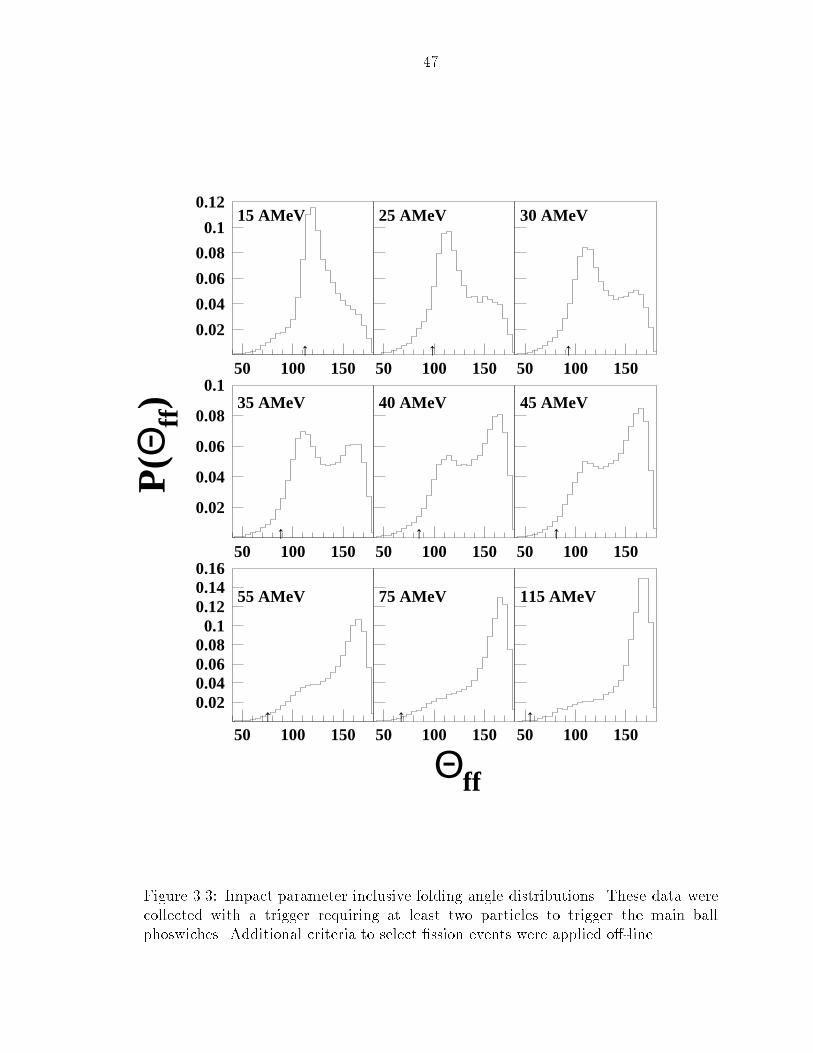
In Figure 3.3, the folding angle distributions are again displayed, but in this case
the data were taken with a di�erent hardware trigger. This trigger (called BALL-
2) required two particles to be detected in the main ball phoswiches in order for
the event to be recorded. This trigger has the e�ect of reducing the contribution of
peripheral collisions, which is helpful as we are interested in isolating central events.
The e�ect of the trigger is obvious in the 15 AMeV case where the low LMT peak is
almost completely absent and the dominant feature is the fusion-�ssion peak. With
the low LMT component suppressed, a shoulder in the distribution that could be the
remainder of a high LMT component is visible even at 115 AMeV, perhaps signifying
that a �ssion-like process is still occurring at this energy. However, we will need to
further exclude the peripheral collisions in order to make this determination.
Figure 3.4 displays the folding angle distributions for central collisions as de�ned
using transverse kinetic energy (ET ). (This method of selecting central collisions
is explained in detail in Appendix A.) The number of events in this distribution is
approximately 10% of the number in the inclusive distribution shown in Figure 3.3.
At all energies, there is a single peak which can be associated with high LMT, �ssion-
like events. If one compares the distributions in Figure 3.4 to those in Figure 3.3 in
which a high LMT component is visible, it is apparent that the peak selected with ET
is in the same place (�110o ) as the high LMT peak in the impact parameter inclusive
distribution. However, as the high LMT peak in Figure 3.3 becomes di�cult to make
out, the peak in Figure 3.4 remains easily distinguishable. Although, this high LMT
component is diminished in absolute size as beam energy increases [Yee 95], this
continuity with the lower energies is strong evidence that a �ssion-like process is still
47
Θff
P(Θ
ff)
15 AMeV
↑
25 AMeV
↑
30 AMeV
↑
35 AMeV
↑
40 AMeV
↑
45 AMeV
↑
55 AMeV
↑
75 AMeV
↑
115 AMeV
↑
0.02
0.04
0.06
0.08
0.1
0.12
50 100 150 50 100 150 50 100 150
0.02
0.04
0.06
0.08
0.1
50 100 150 50 100 150 50 100 150
0.020.040.060.080.1
0.120.140.16
50 100 150 50 100 150 50 100 150
Figure 3.3: Impact parameter inclusive folding angle distributions. These data werecollected with a trigger requiring at least two particles to trigger the main ball
phoswiches. Additional criteria to select �ssion events were applied o�-line.
48
occurring in central events even at 115 AMeV.
There is also some evidence in Figure 3.4 that there is a change in the character of
the high LMT �ssion-like events as beam energy increases. There is a noticeable in-
crease in the width of the distributions with beam energy, although this observation is
made slightly di�cult by the contamination of some target �ssion events on the right
shoulder of the peak. Kinematical broadening can be caused by the emission of other
particles from the nucleus during �ssion or from the daughter fragments after �ssion.
At energies near the Coulomb barrier it is attributed primarily to neutron emission
[Viol 89]. At higher energies, the increased probability of complex fragment emission
[Schw 94, Viol 89] makes this picture more complicated. Asymmetric mass division
between the �ssion fragments can also lead to a tail in the folding angle distribution
extending toward smaller angles [Tsan 83]. Possible changes in the �ssion-like pro-
cesses having to do with the coincident emission of lighter particles will be discussed
in the following sections.
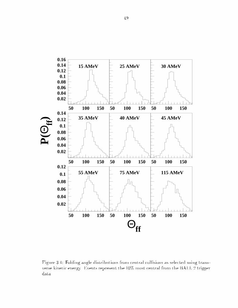
3.3 Azimuthal Distributions
Another characteristic of �ssion that can tell us about the evolution of the reaction
mechanism with beam energy is the relative azimuthal angle between the �ssion
fragments. This angle is depicted in Figure 3.5, and is de�ned to be the angle between
the planes containing each �ssion fragment and the beam axis (�ff). That is, for
perfectly coplanar fragments, �ff is zero, and for fragments perpendicular to one
another, �ff is 90o.
Figure 3.6 illustrates the evolution of �ff with beam energy, for both low LMT
and high LMT collisions, as determined by the folding angle. The dashed curves are
from events containing �ssion fragments with a folding angle between 150oand 180
o,
49
Θff
P(Θ
ff)
15 AMeV 25 AMeV 30 AMeV
35 AMeV 40 AMeV 45 AMeV
55 AMeV 75 AMeV 115 AMeV
0.020.040.060.080.1
0.120.140.16
50 100 150 50 100 150 50 100 150
0.020.040.060.080.1
0.120.14
50 100 150 50 100 150 50 100 150
0.02
0.04
0.06
0.08
0.1
0.12
50 100 150 50 100 150 50 100 150
Figure 3.4: Folding angle distributions from central collisions as selected using trans-
verse kinetic energy. Events represent the 10% most central from the BALL 2 trigger
data.
50
i.e. in the target �ssion peak. These distributions show no change in width as beam
energy increases, giving an indication that there is little change in the character of
these peripheral reactions as beam energy increases. The solid curves are selected
from events in the high LMT peak, and these show signi�cant widening as a function
of beam energy to the point where the distribution is almost at at 115 AMeV.
The widening of the the �ff distributions for high LMT events indicates a change
in the character of the reaction mechanism as beam energy increases much more
dramatically than does the widening of the �ff distributions. The �ff distributions
suggest that the �ssion process is not purely binary at the highest energies. It is well
known that light charged particles emitted either from the nucleus during �ssion or
from the daughter fragments after �ssion can de ect the trajectories of the fragments
out of a common plane with the beam axis [Tsan 84, Viol 89]. However, the degree of
non-coplanarity of the fragments in the highest energy systems studied suggest that
there must be more massive fragments emitted most likely simultaneously with the
�ssion fragments in order for the values �ff to be so drastically altered from zero
[Schw 94]. In the following section we will present evidence that supports this claim
of massive fragment production in conjunction with the �ssion fragments.
3.4 IMF and LCP Production
One of the most fundamental observables one can examine when investigating nuclear
reactions is the production of charged particles. Trends in the mean number of
intermediate mass fragments and light charged particles can provide insights into the
amount of energy that is being deposited into the composite system as beam energy
increases. A large body of evidence links excitation energy deposited in the nucleus
with the production of IMFs [Fiel 86, Troc 89, Pori 89, Ogil 91, deSo 91, Sang 92],
51
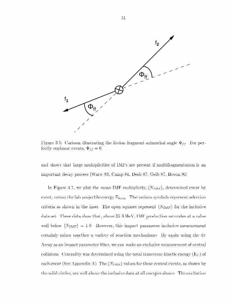
Φff
Φff
f1
f2
Figure 3.5: Cartoon illustrating the �ssion fragment azimuthal angle �ff . For per-
fectly coplanar events, �ff = 0.
and shows that large multiplicities of IMFs are present if multifragmentation is an
important decay process [Warw 83, Camp 84, Desb 87, Gelb 87, Bowm 91].
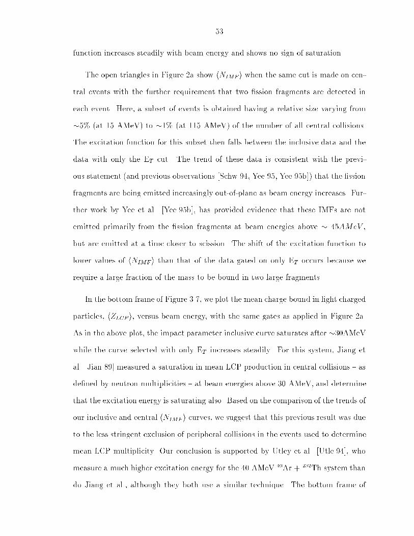
In Figure 3.7, we plot the mean IMF multiplicity, hNIMF i, determined event by
event, versus the lab projectile energy Ebeam. The various symbols represent selection
criteria as shown in the inset. The open squares represent hNIMF i for the inclusivedata set. These data show that, above 35 AMeV, IMF production saturates at a value
well below hNIMF i = 1.0. However, this impact parameter inclusive measurement
certainly mixes together a variety of reaction mechanisms. By again using the 4�
Array as an impact parameter �lter, we can make an exclusive measurement of central
collisions. Centrality was determined using the total transverse kinetic energy (ET ) of
each event (See Appendix A). The hNIMF i values for these central events, as shown bythe solid circles, are well above the inclusive data at all energies shown. The excitation
52
Φff
P(Φ
ff)
15 AMeV 25 AMeV 30 AMeV
35 AMeV 40 AMeV 45 AMeV
55 AMeV 75 AMeV 115 AMeV
0.05
0.1
0.15
-60 0 60 -60 0 60 -60 0 60
0.05
0.1
0.15
-60 0 60 -60 0 60 -60 0 60
0.05
0.1
0.15
-60 0 60 -60 0 60 -60 0 60
Figure 3.6: Fission fragment azimuthal angle �ff distributions for low LMT events
(dashed lines) and high LMT events (solid lines).
53
function increases steadily with beam energy and shows no sign of saturation.
The open triangles in Figure 2a show hNIMF i when the same cut is made on cen-
tral events with the further requirement that two �ssion fragments are detected in
each event. Here, a subset of events is obtained having a relative size varying from
�5% (at 15 AMeV) to �1% (at 115 AMeV) of the number of all central collisions.
The excitation function for this subset then falls between the inclusive data and the
data with only the ET cut. The trend of these data is consistent with the previ-
ous statement (and previous observations [Schw 94, Yee 95, Yee 95b]) that the �ssion
fragments are being emitted increasingly out-of-plane as beam energy increases. Fur-
ther work by Yee et al. [Yee 95b], has provided evidence that these IMFs are not
emitted primarily from the �ssion fragments at beam energies above � 45AMeV ,
but are emitted at a time closer to scission. The shift of the excitation function to
lower values of hNIMF i than that of the data gated on only ET occurs because we
require a large fraction of the mass to be bound in two large fragments.
In the bottom frame of Figure 3.7, we plot the mean charge bound in light charged
particles, hZLCP i, versus beam energy, with the same gates as applied in Figure 2a.
As in the above plot, the impact parameter inclusive curve saturates after �30AMeV
while the curve selected with only ET increases steadily. For this system, Jiang et
al. [Jian 89] measured a saturation in mean LCP production in central collisions { as
de�ned by neutron multiplicities { at beam energies above 30 AMeV, and determine
that the excitation energy is saturating also. Based on the comparison of the trends of
our inclusive and central hNIMF i curves, we suggest that this previous result was dueto the less stringent exclusion of peripheral collisions in the events used to determine
mean LCP multiplicity. Our conclusion is supported by Utley et al. [Utle 94], who
measure a much higher excitation energy for the 40 AMeV 40Ar + 232Th system than
do Jiang et al., although they both use a similar technique. The bottom frame of
54
Et cut only
Et and FF cut
Inclusive
a
<NIM
F>
b
Ebeam [AMeV]
<ZL
CP>
0
0.5
1
1.5
2
2.5
02468
10121416
20 40 60 80 100 120
Figure 3.7: Top frame: Average IMF multiplicities plotted versus beam energy. Thevarious symbols represent criteria used to select subsets of events, and are de�ned
in the inset. Bottom frame: Average charge bound in light charged particles versus
beam energy for the same selection criteria.
55
Figure 3.7 also shows that there is little di�erence between the curve gated on ET and
FFs and the curve gated on only ET . This would seem to indicate an insensitivity of
LCP production to the formation of �ssion fragments versus IMFs in these data.
The steady increase of the curves gated on ET in Figure 3.7 suggests that increas-
ing amounts of energy are being deposited in this system in central collisions. The
evidence of this increase is contrary to the results of at least one previous experiment,
[Jian 89] but in qualitative agreement with several others [Conj 85, Ethv 91, Utle 94].
This observation leaves open the possibility that a change in the dominant reaction
mechanism to multifragmentation could be occurring as beam energy increases. How-
ever this determination is di�cult to make based on IMF multiplicities alone. If a
system of this size is multifragmenting one may expect to see more IMFs on average
than the hNIMF i reached at 115 AMeV, which is less than 2.5. Recent measurements
of the 36Ar + 197Au system have found hNIMF i = 4 in central collisions [deSo 91].
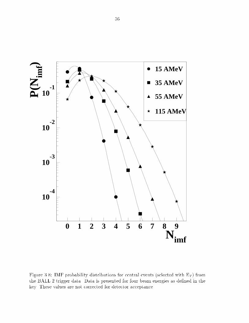
However, at 115 AMeV, the standard deviation of the IMF probability distribution for
central events is quite large (�IMF = 1.3), as can be seen in Figure 3.8. A signi�cant
fraction (�40%) of the central events contains three or more IMFs.
As mentioned in the previous section, there are multiple sources for IMF and LCP
emission, including preequilibrium emission and statistical emission from an fusion-
like source. Work by Fatyga et al. [Faty 87a, Faty 87b], has shown that particles
from these sources can be separated through the selection of emission angle. Based
�ts to energy spectra, Fatyga states that IMFs emitted at backward angles seem to
come from the fusion-like source, whereas particles emitted at more forward angles
are most likely from preequilibrium processes. We have made no such distinction in
the above results, and therefore claim only to be accessing overall deposition energy
thus far, rather than thermal excitation energy.
56
15 AMeV
35 AMeV
55 AMeV
115 AMeV
Nimf
P(N
imf)
10-4
10-3
10-2
10-1
0 1 2 3 4 5 6 7 8 9
Figure 3.8: IMF probability distributions for central events (selected with ET ) from
the BALL 2 trigger data. Data is presented for four beam energies as de�ned in the
key. These values are not corrected for detector acceptance.
57
3.5 Calculations of Momentum Transfer and Ex-
citation Energy
In the previous sections, we have presented measurements of observables which are
related to the momentum transfer and energy deposition in the 40Ar + 232Th system.
In the next sections, we will quantitatively determine these properties, and study
their evolution with bombarding energy.
3.5.1 Linear Momentum Transfer
The momentum transferred to the �ssioning nucleus can be calculated if one measures
the mass and velocity of the �ssion fragments. While these observables were not di-
rectly available for the present analysis, a calculation of the average linear momentum
transfer, relative to the beam momentum hpipbeam
can still be performed as shown in
Reference [Leeg 92],
hpipbeam
=
MhEkiMpEp
!1=2sin�ff
[2sin2(�1) + 2sin2(�2)� sin2(�ff)]1=2; (3:3)
where Mp and Ep are the mass and kinetic energy of the projectile, and M is the
mass of the the �ssioning nucleus. For hEki, the updated formula from Viola was
used [Viol 85]:
hEki = (:1189Z
2
A1=3+ 7:3)MeV: (3:4)
The angles �1 and �2 are the angles of the �ssion fragments with respect to the
trajectory of the �ssioning nucleus. It is assumed this trajectory is the same as the
beam direction, so the lab angles of the �ssion fragments are used for �1 and �2.
The mass M is extrapolated from values measured by Conjeaud et al. [Conj 85] at
energies near the middle of the present range studied. Using equation 3.10, the linear
momentum transfer is calculated event by event, and an average is found.
58
In Figure 3.9, the fractional linear momentum transferpk
pbeamis plotted versus the
velocity parameter [(Ebeam - Ec)/A]1=2. Ec is the Coulomb barrier which is �200 MeV
for this system. The solid line represents a systematic dependence of the momentum
transfer on the beam momentum which has been determined empirically from data
collected by several investigators [Viol 82]. The parameterization used here is from
the work of Nifenecker et al. [Nife 85]. The solid circles represent the most probable
linear momentum transfer, pmp
k , determined by �tting a gaussian to the momentum
transfer distribution from the high LMT events in the most central collisions, i.e., the
events shown in Figure 3.4. In previous experiments with this system, this variable
could not be extracted at energies above 40 AMeV, because the high LMT peak could
not be resolved in the inclusive folding angle distribution [Schw 94]. The values we
extract agree quite well with the systematic curve even at the highest beam energies
where there had been no data previously for this system.
The open squares represent the mean linear momentum transfer, hpki, from the
impact parameter inclusive data in Figure 3.3. These values are always below the
data from the central collisions because of the contribution to the �ssion cross section
from peripheral collisions. The relative size of this contribution increases with beam
energy, and so the discrepancy between the two data sets increases as well.
Figure 3.10 shows the evolution of the linear momentum transfer per projectile
nucleonp
Abeamas a function of the velocity parameter [(Ebeam - Ec)/A]
1=2. The solid
line indicates the beam momentum or full momentum transfer, and the symbol de�-
nitions are the same as in Figure 3.9. The momentum transfer per projectile nucleon
is always less than full beam momentum in this energy range, even for the central
collisions. This indicates, as stated in section 3.2, that primarily incomplete mass
transfer is occurring. The impact parameter inclusive measurement of average mo-
mentum transfer is maximumat 25 AMeV, and then decreases with beammomentum.
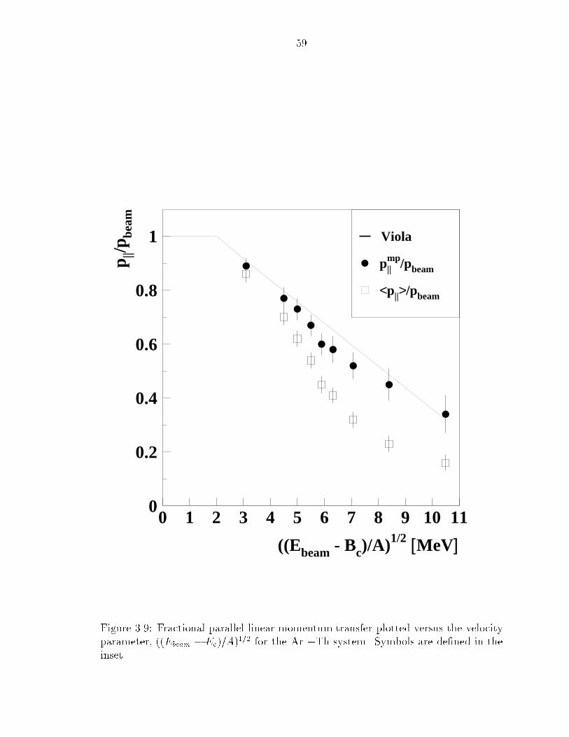
59
((Ebeam - Bc)/A)1/2 [MeV]
p ||/p be
am
<p||>/pbeam
p||mp/pbeam
Viola
0
0.2
0.4
0.6
0.8
1
0 1 2 3 4 5 6 7 8 9 10 11
Figure 3.9: Fractional parallel linear momentum transfer plotted versus the velocity
parameter, ((Ebeam � Ec)=A)1=2 for the Ar +Th system. Symbols are de�ned in the
inset.
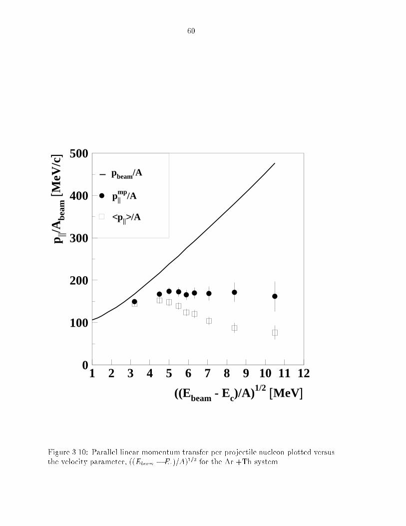
60
((Ebeam - Ec)/A)1/2 [MeV]
p ||/A
beam
[MeV
/c]
<p||>/A
p||mp/A
pbeam/A
0
100
200
300
400
500
1 2 3 4 5 6 7 8 9 10 11 12
Figure 3.10: Parallel linear momentum transfer per projectile nucleon plotted versus
the velocity parameter, ((Ebeam � Ec)=A)1=2 for the Ar +Th system.
61
Both the location of this maximum and the rate of decline of hpiAbeam
beyond that point
are in agreement with data from similar systems [Viol 89, Faty 85].
The momentum transfer for the isolated high LMT events does not decline with
beam energy. The solid points show that it increases with beam energy from 15
AMeV to 25 AMeV and then saturates at approximately 170 MeV/c per projectile
nucleon.
3.5.2 Excitation Energy
As one might expect, linear momentum transfer is closely linked to deposited ex-
citation energy [Jacq 85, Bege 92, Blai 92]. Intranuclear cascade calculations from
the 1960s provided an empirical relationship between these two quantities [Pori 60].
In order to quantitatively determine the energy deposited in the 40Ar + 232Th sys-
tem we performed a calculation of the average total excitation energy, hE�i, using a
method similar to that described in Reference [Bege 92], and based on new calcula-
tions presented in Reference [Blai 92]. In [Bege 92], excitation energy as calculated
through
E� = E
�CF
pkpbeam
AP +AT
Asys
(3:5)
was shown to reasonably describe the mass loss of the �ssioning nucleus. E�CF
rep-
resents the excitation energy for complete fusion, AP and AT are the atomic mass of
the projectile and target, respectively, and Asys is the atomic mass of the �ssioning
system. The quantity E� is calculated from the most probable LMT measured in the
most central �ssion-like reactions (the solid circles in Figure 3.9) using the method
described in the previous section. The average excitation energies, hE�i, extracted inthis way are summarized in Table 3.1. The values we obtained for the energies studied
in Reference [Conj 85] agree well with the values cited in that work. Uncertainties
were calculated from the width of the momentum transfer distributions coupled with
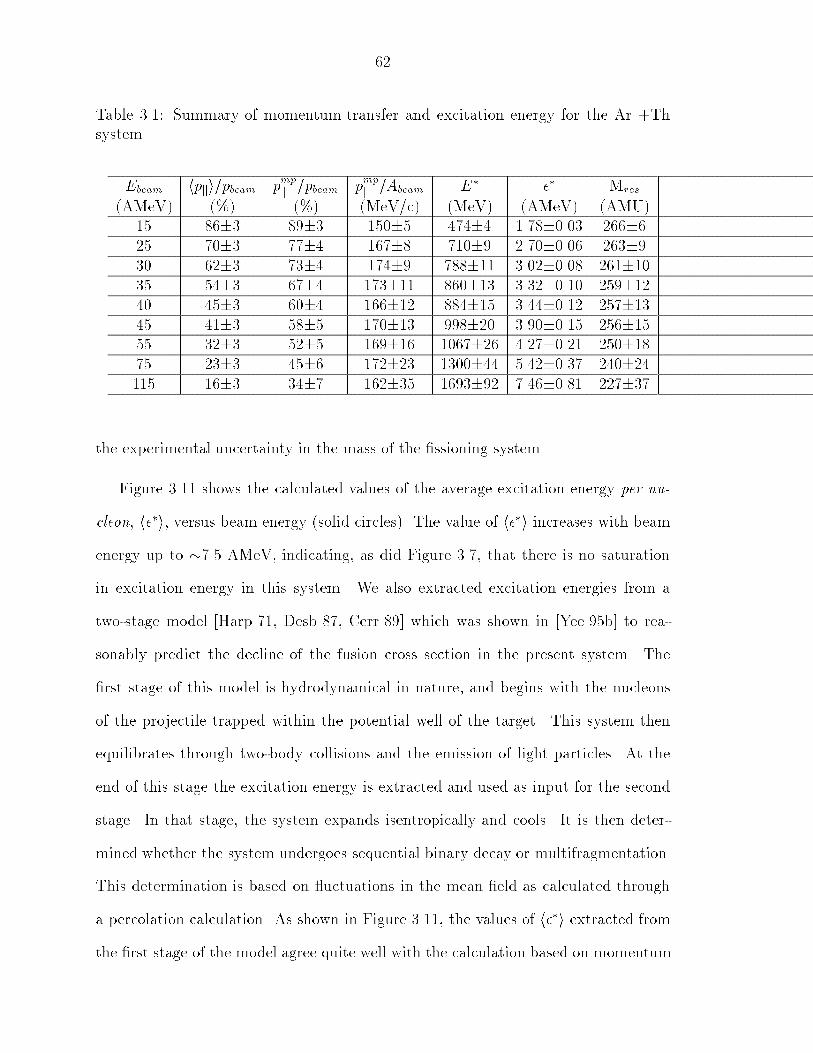
62
Table 3.1: Summary of momentum transfer and excitation energy for the Ar +Th
system.
Ebeam hpki=pbeam pmp
k =pbeam pmp
k =Abeam E�
�� Mres
(AMeV) (%) (%) (MeV/c) (MeV) (AMeV) (AMU)
15 86�3 89�3 150�5 474�4 1.78�0.03 266�625 70�3 77�4 167�8 710�9 2.70�0.06 263�930 62�3 73�4 174�9 788�11 3.02�0.08 261�1035 54�3 67�4 173�11 860�13 3.32�0.10 259�1240 45�3 60�4 166�12 884�15 3.44�0.12 257�1345 41�3 58�5 170�13 998�20 3.90�0.15 256�1555 32�3 52�5 169�16 1067�26 4.27�0.21 250�1875 23�3 45�6 172�23 1300�44 5.42�0.37 240�24115 16�3 34�7 162�35 1693�92 7.46�0.81 227�37
the experimental uncertainty in the mass of the �ssioning system.
Figure 3.11 shows the calculated values of the average excitation energy per nu-
cleon, h��i, versus beam energy (solid circles). The value of h��i increases with beam
energy up to �7.5 AMeV, indicating, as did Figure 3.7, that there is no saturation
in excitation energy in this system. We also extracted excitation energies from a
two-stage model [Harp 71, Desb 87, Cerr 89] which was shown in [Yee 95b] to rea-
sonably predict the decline of the fusion cross section in the present system. The
�rst stage of this model is hydrodynamical in nature, and begins with the nucleons
of the projectile trapped within the potential well of the target. This system then
equilibrates through two-body collisions and the emission of light particles. At the
end of this stage the excitation energy is extracted and used as input for the second
stage. In that stage, the system expands isentropically and cools. It is then deter-
mined whether the system undergoes sequential binary decay or multifragmentation.
This determination is based on uctuations in the mean �eld as calculated through
a percolation calculation. As shown in Figure 3.11, the values of h��i extracted from
the �rst stage of the model agree quite well with the calculation based on momentum
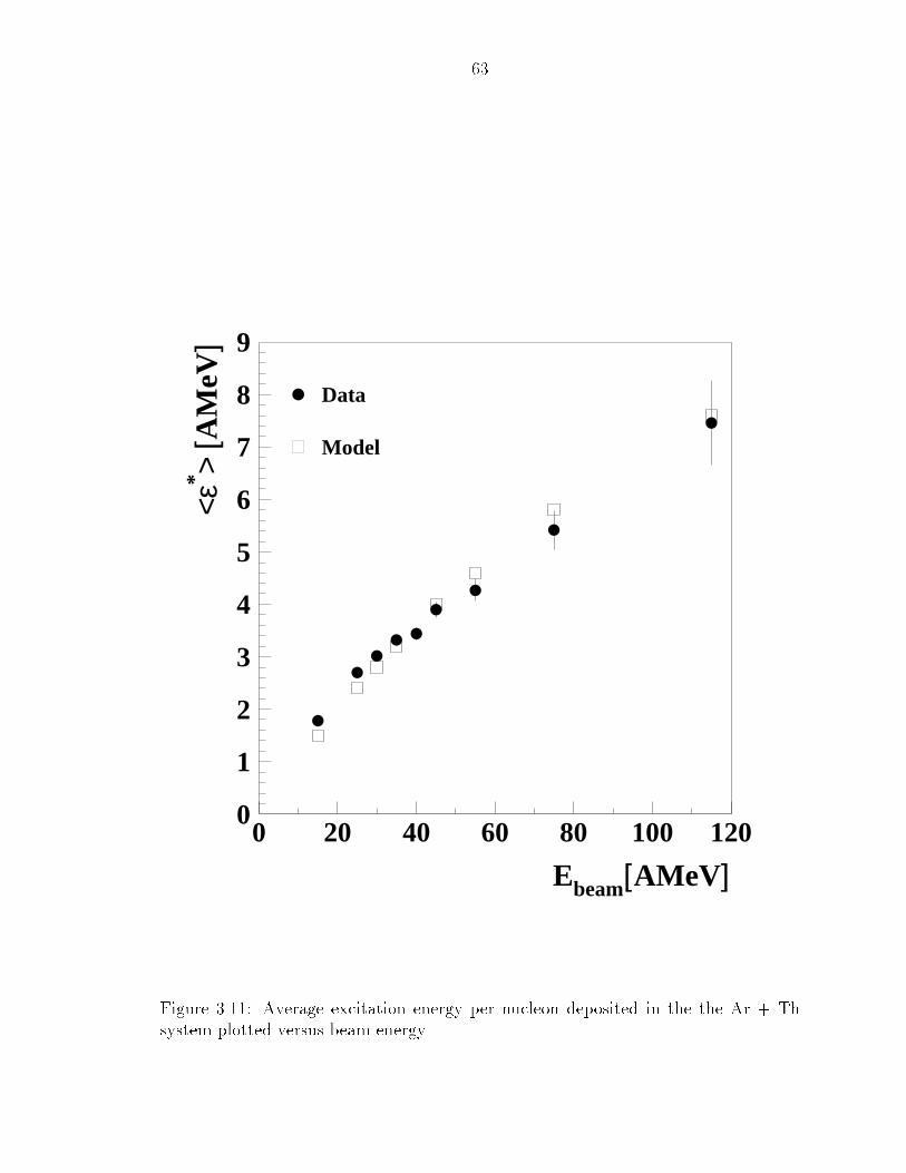
63
Ebeam[AMeV]
<ε* >
[AM
eV]
Data
Model
0
1
2
3
4
5
6
7
8
9
0 20 40 60 80 100 120
Figure 3.11: Average excitation energy per nucleon deposited in the the Ar + Th
system plotted versus beam energy.
64
transfer.
3.6 Summary and Discussion
In this chapter we have studied the evolution of �ssion fragment angular distributions,
momentum transfer and excitation energy in 40Ar + 232Th collisions, as bombarding
energy is increased from 15 to 115 AMeV. Fission fragment folding angle distributions
support previous measurements that indicate the process of fusion-�ssion declines
with bombarding energy. However, through the use of impact parameter �lters, we
have determined that a high LMT, �ssion-like process still occurs even at 115 AMeV.
Fission fragment azimuthal distributions indicate that the nature of the �ssion at
these energies has changed from an essentially binary to a many-fragment process.
Momentum transfer per projectile nucleon in high LMT, �ssion-like events has
been found to saturate at 170 MeV/c for beam energies above 30 AMeV. Fractional
momentum transfer for these events has been found to agree quite well with an
empirically determined functional form for all beam energies studied, including the
highest energies for which this variable has not been measured before in this system.
The saturation of momentum transfer as it approaches the value of the Fermi mo-
mentum (�250 MeV/c [Moni 71]) has been interpreted as indicating the increased
e�ect of nucleon-nucleon interactions over the in uence of the dinuclear mean-�eld
[Jacq 84, Faty 85, Viol 89].
Energy deposited in this system in central collisions has been shown to increase
steadily with beam energy through the measurement of IMF and LCP multiplicities
as well as through a calculation involving the measured momentum transfer. These
observations about momentum transfer and deposited energy lead one to ask if the
dominant reaction mechanism is changing as beam energy increases. In the Ar +

65
Au system, for example, evidence has been presented there is a possible transition to
multifragmentation at excitation energies of 5 AMeV, a value we reach in this system
at bombarding energies near 55 - 75 AMeV [Biza 93]. In the next chapter we present
evidence for a similar transition in this system.

66
Chapter 4
Event Shape Analysis
4.1 Introduction
This chapter will discuss changes in the reaction mechanism in 40Ar + 232Th collisions
as function of beam energy, as viewed through the technique of event shape analysis
[Cugn 82, Gyul 82, Cebr 90a, Cebr 91]. Topics that will be dealt with include mul-
tiplicity distortions inherent in this method, the e�ects of detector acceptance, and
the separation of projectile-like sources from center-of-mass sources.
4.2 The Flow Tensor
The event shape analysis begins with the event by event construction of the ow
tensor [Cugn 82, Gyul 82]. Each event is transformed into the center-of-mass reference
frame, and the ow tensor is then constructed by summing over the momentum
components of each fragment in the event as follows:
F =Xi;j
Fij (4:1)
where
Fij =NcXn=1
!npi
npj
n: (4:2)
67
68
The sum runs over the total event multiplicity Nc, and the variables i and j represent
the cartesian coordinates x, y, and z. Thus, the quantity pinis the ith momentum
component of the nth particle in the event. The quantity !n is the weighting factor for
each particle and is needed to make the tensor coalescence invariant. That is, since
the sum runs over particles of various masses, a factor must be included to ensure
that heavy fragments do not dominate the ow tensor. This factor is often chosen to
be 12mn
, making F the kinetic energy tensor, however 1p2n
is also a valid choice. The
end result is an ellipsoid that describes either the energy or particle ow of the event.
Once the tensor is constructed, an orthogonal similarity transformation is per-
formed to reduce it to diagonal form. This corresponds to rotating the coordinate
axes so that they coincide with the principal axes of the three-dimensional momen-
tum spheroid. The ellipsoid can be completely described by three eigenvalues (fi) and
three eigenvectors (ei):
F = f1e1e1y + f2e2e2
y + f3e3e3y; (4:3)
where the eigenvectors give the direction of the principal axes, and the square root
of the eigenvalues (pfi) give the length of those axes. Figure 4.1 depicts such an
ellipsoid. It is extremely important that the tensor be constructed in the frame of the
emitting source. If the frame of calculation moves quickly with respect to the emitting
frame, all of the momentum vectors will appear elongated due to the relative motion
of the source and the ellipsoid will thus be arti�cially elongated as well.
The eigenvalues of the tensor satisfy the cubic equation
f3i+ a2f
2i+ a1fi + a0 = 0; (4:4)
with
a2 = �(F11 + F22 + F33); (4:5)
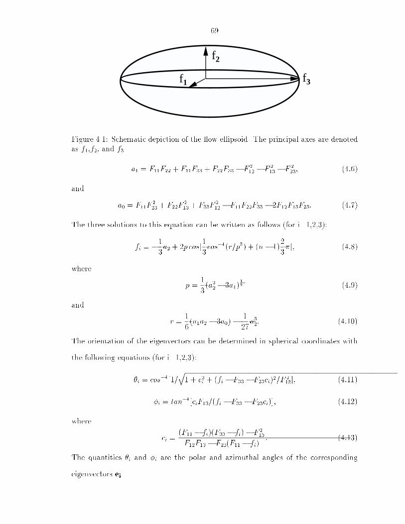
69
f2
f3f1
Figure 4.1: Schematic depiction of the ow ellipsoid. The principal axes are denotedas f1,f2, and f3
a1 = F11F22 + F11F33 + F22F33 � F212 � F
213 � F
223; (4:6)
and
a0 = F11F223 + F22F
213 + F33F
212 � F11F22F33 � 2F12F13F23: (4:7)
The three solutions to this equation can be written as follows (for i=1,2,3):
fi = �1
3a2 + 2p cos[
1
3cos
�1(r=p3) + (n� 1)2
3�]; (4:8)
where
p =1
3(a22 � 3a1)
1
2 (4:9)
and
r =1
6(a1a2 � 3a0)� 1
27a32: (4:10)
The orientation of the eigenvectors can be determined in spherical coordinates with
the following equations (for i=1,2,3):
�i = cos�1[1=
q1 + c
2i + (fi � F33 � F23ci)2=F 2
13]; (4:11)
�i = tan�1[ciF13=(fi � F33 � F23ci)]; (4:12)
where
ci =(F11 � fi)(F33 � fi)� F
213
F12F13 � F23(F11 � fi): (4:13)
The quantities �i and �i are the polar and azimuthal angles of the corresponding
eigenvectors ei.
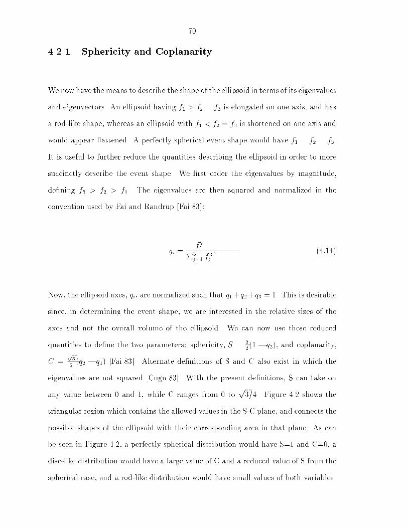
70
4.2.1 Sphericity and Coplanarity
We now have the means to describe the shape of the ellipsoid in terms of its eigenvalues
and eigenvectors. An ellipsoid having f1 > f2 = f3 is elongated on one axis, and has
a rod-like shape, whereas an ellipsoid with f1 < f2 = f3 is shortened on one axis and
would appear attened. A perfectly spherical event shape would have f1 = f2 = f3.
It is useful to further reduce the quantities describing the ellipsoid in order to more
succinctly describe the event shape. We �rst order the eigenvalues by magnitude,
de�ning f3 > f2 > f1. The eigenvalues are then squared and normalized in the
convention used by Fai and Randrup [Fai 83]:
qi =f2iP3
j=1 f2j
: (4:14)
Now, the ellipsoid axes, qi, are normalized such that q1+q2+q3 = 1. This is desirable
since, in determining the event shape, we are interested in the relative sizes of the
axes and not the overall volume of the ellipsoid. We can now use these reduced
quantities to de�ne the two parameters: sphericity, S = 32(1 � q3), and coplanarity,
C =p32(q2 � q1) [Fai 83]. Alternate de�nitions of S and C also exist in which the
eigenvalues are not squared [Cugn 83]. With the present de�nitions, S can take on
any value between 0 and 1, while C ranges from 0 top3=4. Figure 4.2 shows the
triangular region which contains the allowed values in the S-C plane, and connects the
possible shapes of the ellipsoid with their corresponding area in that plane. As can
be seen in Figure 4.2, a perfectly spherical distribution would have S=1 and C=0, a
disc-like distribution would have a large value of C and a reduced value of S from the
spherical case, and a rod-like distribution would have small values of both variables.
71
Sphericity
Cop
lana
rity
Disk
SphereRod Prolate
Oblate
Tri-axial
Oval
0
0.05
0.1
0.15
0.2
0.25
0.3
0.35
0.4
0 0.1 0.2 0.3 0.4 0.5 0.6 0.7 0.8 0.9 1
Figure 4.2: Diagram de�ning the allowed region of S-C space. Shapes along theline connecting (0,0) and (0.75,0.43) are 2-dimensional and range from a perfect rod(f2 = f3 = 0) to a perfect circle (f3 = f2 =
12; f1 = 0). Shapes along the bottom axis
range from a perfect rod to a sphere (f1 = f2 = f3 =13) with f2 and f3 increasing
with sphericity. Shapes on the line from (0.75,0.43) to (0,1) range from a perfect
circle to a sphere, with f1 increasing as coplanarity decreases.
72
4.3 Relationship of the Event Shape to the Re-
action Mechanism
In section 4.2 the basis of the technique of event shape analysis was described. In this
section, we will relate the usefulness of this technique to the study of the evolution
of the reaction mechanism in 40Ar + 232Th collisions.
L�opez and Randrup have proposed that the shape of the ow tensor should be
sensitive to the timescale of the breakup process [Lope 89]. At beam energies well
below the Fermi energy, the sequential decay of particles is known be the dominant
breakup process [Gelb 87]. This type of time-ordered process should lead to elongated
event shapes due to the kinematical constraints of the fragment emission. That is, the
compound nucleus emits a particle and recoils, that particle then emits another and
so on. The trajectories of the subsequently emitted particles are in uenced strongly
by the initial axis of emission.
At beam energies above the Fermi energy, multifragmentation processes are be-
lieved to become dominant [Fai 83, Bond 90, Bowm 91, Ogil 91]. These processes
occur on a much faster time scale than sequential processes and are characterized by
the nearly simultaneous breakup of the colliding system into many intermediate size
particles. In this scenario, the emission of the fragments may be isotropic as there
are no longer one or two large fragments to de�ne an axis [Cebr 90a, Ogil 91].
As discussed in the previous chapter, in the 40Ar + 232Th system at beam energies
below �40 AMeV, it is known that the fusion-�ssion process dominates the cross sec-
tion [Viol 89, Viol 82, Conj 85]. In the frame of the �ssioning nucleus, the two �ssion
fragments are emitted roughly back-to-back as required by momentum conservation,
and their trajectories de�ne the �ssion axis. While particles may be emitted isotrop-
ically from the daughter fragments, their momenta in the frame of the compound
73
nucleus will be folded toward the �ssion axis. A study by Yee et al., has shown that
the emission angles of particles with charge Z=2 and higher are highly correlated with
the trajectory of either of the �ssion fragments in this system at energies below 40
AMeV [Yee 95b].
The �ssion plane is formed by the �ssion axis and the beam axis. Work by Tsang
et al. has shown that light and intermediate mass charged particles are emitted pref-
erentially in the �ssion plane for systems similar to the present one. This anisotropy
was shown to increase with the mass and kinetic energy of the emitted particles
[Tsan 84, Tsan 90, Tsan 91]. These types of focussing e�ects will suppress sphericity
since the ellipsoid described by the ow tensor will be attened towards the �ssion
plane and elongated along the �ssion axis.
At the highest energies studied here (>50 AMeV), it has been suggested that
multifragmentation takes over as the dominant reaction mechanism [Conj 85, Viol 89,
Schw 94]. In this case, the emission may be isotropic, and sphericity should be close
to the maximum value allowed. Work by Wilson et al. [Wils 91] has shown that
for symmetric systems, the aforementioned anisotropy all but disappears for beam
energies near 100 AMeV, providing a clue that the reaction mechanism is undergoing
a transition. In asymmetric systems, polar angle distributions of complex fragments
indicate increasingly isotropic emission as excitation energy increases [Yenn 90]. Like
the decline of this anisotropy, an increase in sphericity may also be interpreted as a
signal that there has been a change in the dominant reaction mechanism from fusion-
�ssion to multifragmentation. However, there are some issues that must be discussed
before this connection can be made.
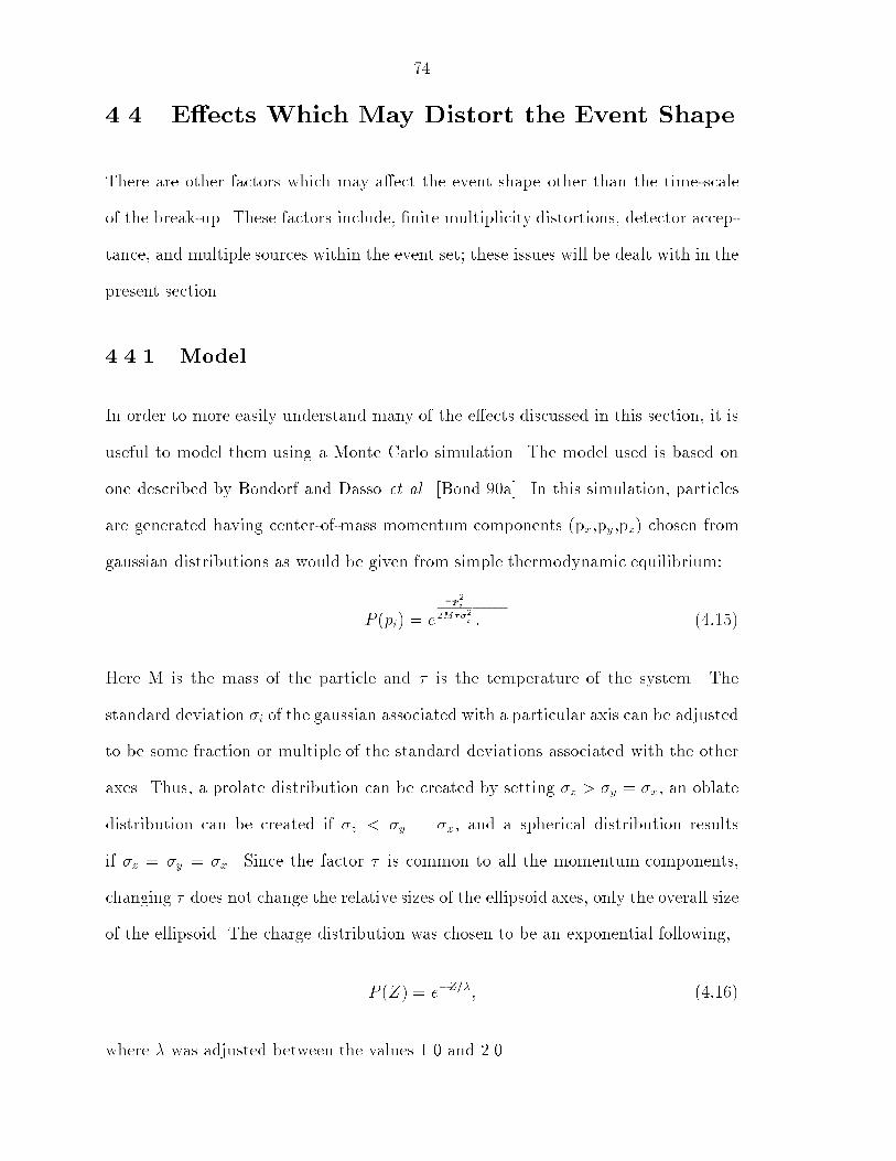
74
4.4 E�ects Which May Distort the Event Shape
There are other factors which may a�ect the event shape other than the time-scale
of the break-up. These factors include, �nite multiplicity distortions, detector accep-
tance, and multiple sources within the event set; these issues will be dealt with in the
present section.
4.4.1 Model
In order to more easily understand many of the e�ects discussed in this section, it is
useful to model them using a Monte Carlo simulation. The model used is based on
one described by Bondorf and Dasso et al. [Bond 90a]. In this simulation, particles
are generated having center-of-mass momentum components (px,py,pz) chosen from
gaussian distributions as would be given from simple thermodynamic equilibrium:
P (pi) = e
�p2i
2M��2i : (4:15)
Here M is the mass of the particle and � is the temperature of the system. The
standard deviation �i of the gaussian associated with a particular axis can be adjusted
to be some fraction or multiple of the standard deviations associated with the other
axes. Thus, a prolate distribution can be created by setting �z > �y = �x, an oblate
distribution can be created if �z < �y = �x, and a spherical distribution results
if �z = �y = �x. Since the factor � is common to all the momentum components,
changing � does not change the relative sizes of the ellipsoid axes, only the overall size
of the ellipsoid. The charge distribution was chosen to be an exponential following,
P (Z) = e�Z=�
; (4:16)
where � was adjusted between the values 1.0 and 2.0.
75
A set of 50,000 events with multiplicity Nc=10, and temperature � = 6 MeV was
generated from a prolate momentum distribution with 2�x = 2�y = �z = 2, and a
summary of this event set is shown in Figure 4.3. The frame of the emitting source
was at rest in the lab. The frames in Figure 4.3 contain plots of key aspects of the
simulated events as described in the �gure caption. Shown explicitly in this �gure is
the e�ect of making �z largest of the three standard deviations, since the projection
of the momentum distribution along the z-axis (Pz) is much wider that along the
y-axis (Py).
In the bottom right frame of Figure 4.3, the mean value of sphericity, hSi, for theevent set is plotted versus the velocity of the frame in which the momentum tensor
was constructed. This demonstrates the e�ect of constructing the momentum tensor
in a frame other than the emitting frame. The frame is boosted along the z-axis and
this induces an apparent elongation of the momentum ellipsoid in the boost direction.
Thus, the value of hSi diminishes as we leave �frame = 0. The sphericity probability
distributions for the correct frame are shown in the bottom left frame of Figure 4.3.
These two frames demonstrate another important aspect of the the sphericity
measurement. This aspect is the di�erence in hSi when the 1p2
normalization is used
for the ow tensor elements as opposed to the 12m
normalization. In the former case,
all of the momentum vectors are made into unit vectors, thus, hSi must necessarilybe larger than in the latter case because all of the vectors now lie with their ends on a
sphere. Only the directions of the particle momenta matter with this normalization;
variations in particle energy have no e�ect on the sphericity. The usefulness of this
feature will be made apparent in section 4.4.3.
76
Z
P(Z
)
Eα (MeV)
P(E
α)
Py (MeV/c)
P(P
y)
Pz (MeV/c)
P(P
z)
S
P(S
)
Nc = 10
βframe
<S>
1/p2 1/2m
10-4
10-3
10-2
10-1
1
2 4 6 8 10
10-4
10-3
10-2
10-1
0 50 100 150 200
10-5
10-4
10-3
10-2
-1000 -500 0 500 1000
10-4
10-3
10-2
-1000 -500 0 500 1000
0
0.02
0.04
0.06
0.08
0.1
0 0.2 0.4 0.6 0.8 10
0.2
0.4
0.6
-0.2 0 0.2 0.4 0.6
Figure 4.3: Set of 50,000 events with multiplicity Nc = 10 and � = 6 MeV. 2�x =
2�y = �z = 2. The source of the emitting frame was at rest in the lab. The framescontain \snapshots" of key aspects of the simulated events as follows: Z probability
distribution (top left), energy probability distribution for alpha particles (top right),y-axis component of the momentum distribution (middle left), z-axis component of
the momentum distribution (middle right), sphericity distributions as calculated in
the rest frame with 12m
(solid) and 1p2
(dashed) normalizations (bottom left), and the
average sphericity for the event set as calculated for several di�erent boost frameswith both normalizations. The boost direction is along the z-axis.
77
4.4.2 Multiplicity Distortions
It is well known that there are �nite multiplicity distortions that a�ect the measured
values of sphericity [Dani 83, Bond 90a]. For events with a �nite number of particles,
measurements of sphericity will uctuate about an average value which is shifted
from the theoretical value by a factor of order 1/pNc. For events with multiplicities
of Nc > 200, this e�ect is small, however, for particle multiplicities on the order of
those in the present study, it is extremely important. In our case, this means that
completely isotropic event may yield a value of sphericity signi�cantly less than 1.0.
The average value of sphericity for a set of such events may be equivalent to the value
of sphericity corresponding to a prolate event with an in�nite number of particles As
multiplicity increases, and the distortion becomes less important, the measured value
of hSi for these isotropic events begins to increase towards its theoretical (in�nite
particle) value. This means that a simple increase in multiplicity will have the same
e�ect on sphericity as a change to a more spherical emission pattern of the particles.
This could be falsely interpreted as indicating a change in the particle ow and
reaction dynamics.
This e�ect has been simulated in Figure 4.4 using the above mentioned Monte
Carlo model. Events were generated with a prolate (rod-like), oblate (disc-like), or
spherical distribution for event multiplicities Nc = 2 � 20. The input parameters �x,
�y, and �z are chosen as in Bondorf et al. [Bond 90a]. In Figure 4.4a, as Nc increases,
so does hSi for the disk-like and spherical distributions. The rod-like distribution
increases and then attens. Even for events with Nc = 20, the value of hSi for thespherical events is much less 1.0.
For multiplicities below Nc = 5, values of hSi for the three shapes are very close toone another, however, as Figure 4.4b shows, there are measurable di�erences in hSi
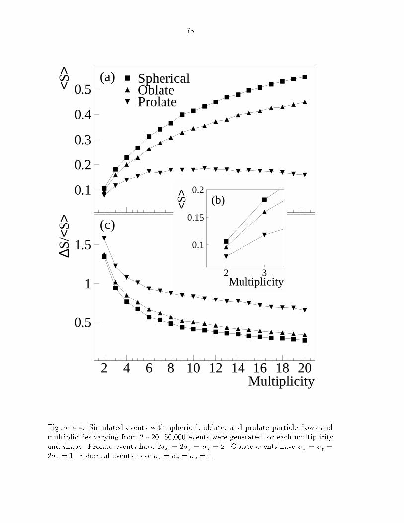
78
0.1
0.2
0.3
0.4
0.5
0.5
1
1.5
2 4 6 8 10 12 14 16 18 20
<S>
SphericalOblateProlate
(a)
Multiplicity
∆S/<
S> (c)0.1
0.15
0.2
2 3Multiplicity
<S>
(b)
Figure 4.4: Simulated events with spherical, oblate, and prolate particle ows andmultiplicities varying from 2 - 20. 50,000 events were generated for each multiplicity
and shape. Prolate events have 2�x = 2�y = �z = 2. Oblate events have �x = �y =
2�z = 1. Spherical events have �x = �y = �z = 1.
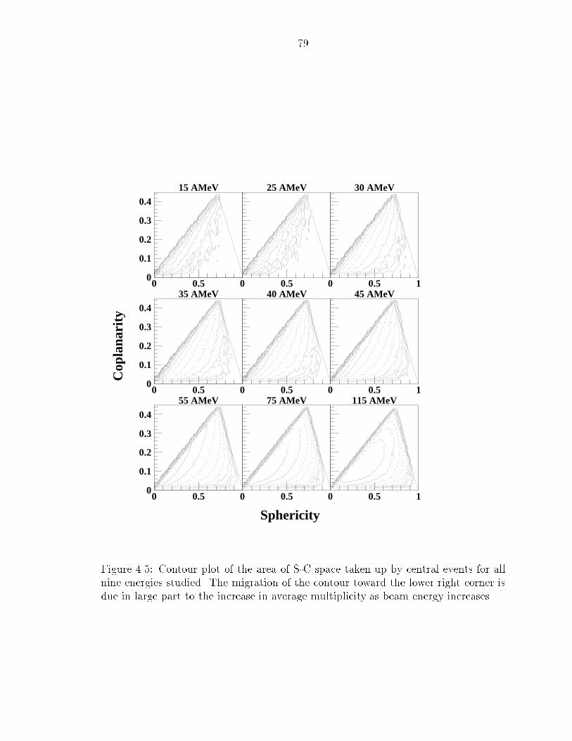
79
Sphericity
Cop
lana
rity
15 AMeV 25 AMeV 30 AMeV
35 AMeV 40 AMeV 45 AMeV
55 AMeV 75 AMeV 115 AMeV
0
0.1
0.2
0.3
0.4
0 0.5 0 0.5 0 0.5 1
0
0.1
0.2
0.3
0.4
0 0.5 0 0.5 0 0.5 1
0
0.1
0.2
0.3
0.4
0 0.5 0 0.5 0 0.5 1
Figure 4.5: Contour plot of the area of S-C space taken up by central events for all
nine energies studied. The migration of the contour toward the lower right corner is
due in large part to the increase in average multiplicity as beam energy increases.
80
even for Nc = 2. Figure 4.4c shows the reduced widths of the sphericity distributions
�S=hSi. The widths decrease steadily with multiplicity as they are also caused by
�nite number uctuations, and would vanish for an in�nite number of particles.
The e�ect of multiplicity distortions can also be seen in the present data as shown
in Figure 4.5. This �gure depicts the S-C distributions for central collisions at the
nine beam energies studied. There is no explicit selection on speci�c multiplicities,
and the shift of the contour toward the lower right corner is due in great part to
the increase in average multiplicity with beam energy. This problem of multiplicity
distortions will be dealt with in the present analysis by explicitly separating events
based on their multiplicity and comparing changes in sphericity only for events that
have the same multiplicity.
4.4.3 Multiple Emitting Sources
It has already been stated that in order for the sphericity analysis to be meaningful,
the ow tensor must be constructed in the correct frame, i.e., the frame in which the
particles are being emitted. This naturally brings up the question of what happens
when there is more than one emitting source in an event or when events in which
the source velocity is di�erent are included in the average over sphericity. We will
begin to deal with these issues using our Monte Carlo model. Figure 4.6 shows the
event summary for 50,000 events generated with two spherically emitting sources.
One source is at rest and the other source is moving with a velocity of � = 0.2c along
the z-axis. Each event contains 20 particles, 10 from each source, and both sources
were given a temperature � = 6 MeV for the sake of symmetry. The double humped
energy distribution and Pz distribution are the trivial result of this two-source event
set. The interesting result is in the plot of hSi versus �frame.
For the 12m
normalization, hSi peaks at a frame velocity halfway between the
81
frames of the two sources. Also, the maximum value of hSi attained is less than the
case of one spherical source with 20 or even 10 particles (see Figure 4.4). Looking
from the frame of the source at rest, the momenta originating from the moving source
are elongated along the z-axis, and this reduces the rest source's sphericity in its own
frame. The inverse of this is true looking from the moving frame as well. Since the
two sources are symmetric, a maximum is reached halfway between the two frames
where the combined elongation e�ect is minimized for both sources.
For the 1p2
normalization, the e�ect is quite di�erent. Since only the emission
angles of the particles are important and not the magnitudes of the momenta, the
sources do not interfere with each other nearly as much as with the other normaliza-
tion, and there are two distinct peaks located at the correct frame velocities. The
two sources do still a�ect one another however, as the maximum value of hSi is stillless than if there were only one spherical source emitting 10 particles.
A simulation was also run in which the two spherical sources are isolated in sepa-
rate events. Half of the events contain the source at rest, and half contain the moving
source. Figure 4.7 shows the summary for this set of events. In this case either nor-
malization provides two distinct peaks at the correct frame velocities in the hSi versus�frame plot. The sphericity probability distributions in the lower left frame also show
two peaks coming from the two distinct groups of events. While the maximum values
of hSi are still lower than the case of one spherically emitting source of 20 particles,
the averaging over two sources in di�erent events does not have as large an e�ect on
hSi as does averaging over two sources in the same event.
In the present data, we are interested in studying the evolution of central collisions
in which the emitting source is presumed to be moving at close to the center-of-mass
velocity. Clearly, if there is a contribution from particles emitted from a faster frame,
as in either of the previous scenarios, this will have an e�ect on the sphericity measure-
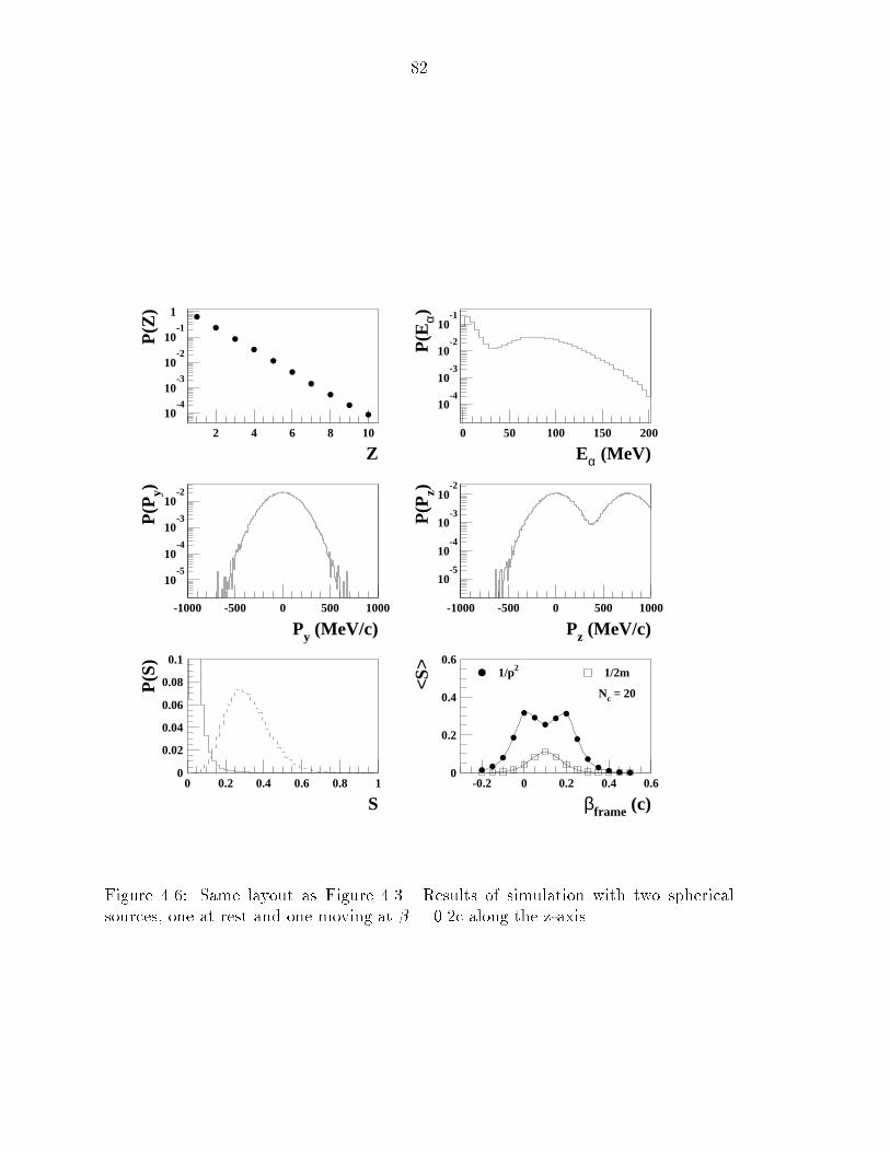
82
Z
P(Z
)
Eα (MeV)
P(E
α)
Py (MeV/c)
P(P
y)
Pz (MeV/c)
P(P
z)
S
P(S
)
Nc = 20
βframe (c)
<S>
1/p2 1/2m
10-4
10-3
10-2
10-1
1
2 4 6 8 10
10-4
10-3
10-2
10-1
0 50 100 150 200
10-5
10-4
10-3
10-2
-1000 -500 0 500 1000
10-5
10-4
10-3
10-2
-1000 -500 0 500 1000
0
0.02
0.04
0.06
0.08
0.1
0 0.2 0.4 0.6 0.8 10
0.2
0.4
0.6
-0.2 0 0.2 0.4 0.6
Figure 4.6: Same layout as Figure 4.3. Results of simulation with two sphericalsources, one at rest and one moving at � = 0.2c along the z-axis.
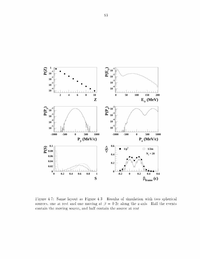
83
Z
P(Z
)
Eα (MeV)
P(E
α)
Py (MeV/c)
P(P
y)
Pz (MeV/c)
P(P
z)
S
P(S
)
Nc = 20
βframe (c)
<S>
1/p2 1/2m
10-4
10-3
10-2
10-1
1
2 4 6 8 10
10-4
10-3
10-2
10-1
0 50 100 150 200
10-5
10-4
10-3
10-2
-1000 -500 0 500 1000
10-5
10-4
10-3
10-2
-1000 -500 0 500 1000
0
0.02
0.04
0.06
0.08
0.1
0 0.2 0.4 0.6 0.8 10
0.2
0.4
0.6
-0.2 0 0.2 0.4 0.6
Figure 4.7: Same layout as Figure 4.3. Results of simulation with two spherical
sources, one at rest and one moving at � = 0.2c along the z-axis. Half the events
contain the moving source, and half contain the source at rest.
84
ment. This e�ect will be dealt with in two ways: selecting events based on variables
known to be related to impact parameter and the careful choice of normalization for
the ow tensor.
Figure 4.8 shows plots of hSi versus �frame for four of the incident energies studied.
The data in these plots were taken with the trigger requiring two particles to be
detected in the main ball phoswiches (BALL-2 trigger). Other than this hardware
requirement, the data are impact parameter inclusive. The normalization used for
the ow tensor is 12m.
The data have been sorted into subsets based on the multiplicity of charged par-
ticles detected and fully identi�ed (Nc) in each event. Particles detected with the
MWPCs are not included here. The di�erent curves in each plot represent these
subsets as indicated by the various symbols superimposed on them (see key). Each
multiplicity curve has a shape somewhat reminiscent of the curves generated by the
model. That is, there are two peaks (or at least one peak with a large shoulder),
one closer to the center-of-mass frame, and one closer to the projectile frame for each
energy. We can interpret this as evidence that there is more than one source con-
tributing to these events, as would be expected for impact parameter inclusive data.
Notice that the peak at the lower velocity is somewhat to the right of the center-of-
mass velocity, while we might expect it occur at exactly that velocity. Most likely
this shift is caused by the other source moving at the faster velocity, as described
with the simulation. Our �rst step must be to try to reduce the contribution from
this faster source.
In Figure 4.9 mean sphericity versus frame velocity is again shown, but this time
only for the 10%most central collisions as determined using the total transverse charge
of the event. (Choice of this centrality variable is discussed in Appendix A.) In this
�gure, The peak at the faster velocities is signi�cantly reduced in size, indicating that
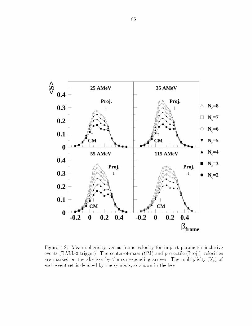
85
βframe
<S>
Nc=2
Nc=3
Nc=4
Nc=5
Nc=6
Nc=7
Nc=8
25 AMeV
Proj.↓
↑CM
35 AMeV
Proj.↓
↑CM
55 AMeV
Proj.↓
↑CM
115 AMeV
Proj.↓
CM↑
0
0.1
0.2
0.3
0.4
0
0.1
0.2
0.3
0.4
-0.2 0 0.2 0.4 -0.2 0 0.2 0.4
Figure 4.8: Mean sphericity versus frame velocity for impact parameter inclusive
events (BALL-2 trigger). The center-of-mass (CM) and projectile (Proj.) velocitiesare marked on the abscissa by the corresponding arrows. The multiplicity (Nc) of
each event set is denoted by the symbols, as shown in the key.
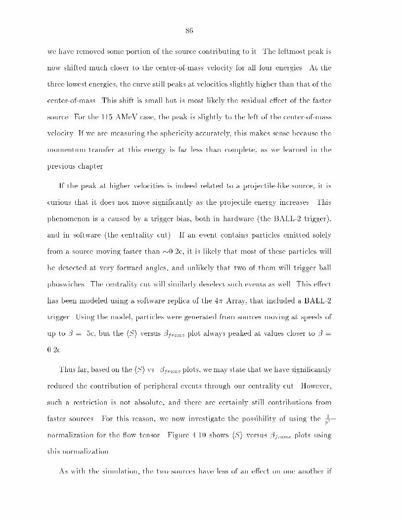
86
we have removed some portion of the source contributing to it. The leftmost peak is
now shifted much closer to the center-of-mass velocity for all four energies. At the
three lowest energies, the curve still peaks at velocities slightly higher than that of the
center-of-mass. This shift is small but is most likely the residual e�ect of the faster
source. For the 115 AMeV case, the peak is slightly to the left of the center-of-mass
velocity. If we are measuring the sphericity accurately, this makes sense because the
momentum transfer at this energy is far less than complete, as we learned in the
previous chapter.
If the peak at higher velocities is indeed related to a projectile-like source, it is
curious that it does not move signi�cantly as the projectile energy increases. This
phenomenon is a caused by a trigger bias, both in hardware (the BALL-2 trigger),
and in software (the centrality cut). If an event contains particles emitted solely
from a source moving faster than �0.2c, it is likely that most of these particles will
be detected at very forward angles, and unlikely that two of them will trigger ball
phoswiches. The centrality cut will similarly deselect such events as well. This e�ect
has been modeled using a software replica of the 4� Array, that included a BALL-2
trigger. Using the model, particles were generated from sources moving at speeds of
up to � = .5c, but the hSi versus �frame plot always peaked at values closer to � =
0.2c.
Thus far, based on the hSi vs. �frame plots, we may state that we have signi�cantly
reduced the contribution of peripheral events through our centrality cut. However,
such a restriction is not absolute, and there are certainly still contributions from
faster sources. For this reason, we now investigate the possibility of using the 1p2
normalization for the ow tensor. Figure 4.10 shows hSi versus �frame plots using
this normalization.
As with the simulation, the two sources have less of an e�ect on one another if
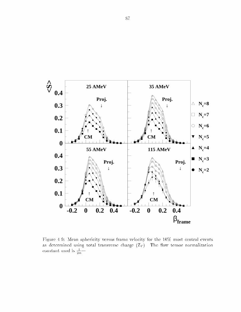
87
βframe
<S>
Nc=2
Nc=3
Nc=4
Nc=5
Nc=6
Nc=7
Nc=8
25 AMeV
Proj.↓
↑CM
35 AMeV
Proj.↓
↑CM
55 AMeV
Proj.↓
↑CM
115 AMeV
Proj.↓
CM↑
0
0.1
0.2
0.3
0.4
0
0.1
0.2
0.3
0.4
-0.2 0 0.2 0.4 -0.2 0 0.2 0.4
Figure 4.9: Mean sphericity versus frame velocity for the 10% most central eventsas determined using total transverse charge (ZT ). The ow tensor normalization
constant used is 12m.
88
we use 1p2, and we can see this in the change in the relative size of the two peaks.
There is a much greater change in the size of the faster component relative to the
change in the size of the center-of-mass component. This may be attributable to the
fact that fewer particles in the event set should be coming from this more peripheral
source because we are selecting central collisions. When we reduce the in uence of the
center-of-mass source on this smaller source by using the 1p2
normalization, there is a
large change in the sphericity. Conversely, we can infer that removing the in uence of
the faster source on the center-of-mass source has a smaller but qualitatively similar
e�ect. For this reason, we determine that the 1p2
normalization is superior in cases
when the source of interest cannot be completely isolated.
4.4.4 Detector Acceptance E�ects
An attempt must always be made to determine the extent to which detector accep-
tance e�ects alter the data. In studies like the present one in which observables are
being measured over a wide range of beam energies, these acceptance e�ects may
change as the velocity of the emitting source changes. In this study in particular,
we are interested in learning if the acceptance will distort the event shape, e.g., will
a \rod" become a \sphere" or vice versa, and if this distortion change with beam
energy.
We again call on our model to aid in this determination. Nine sets of events
with with a spherical momentum distribution (�z = �x = �y=1), were generated
and boosted to the velocity corresponding to the centers-of-mass of the nine systems
studied. These events were then �ltered through a software replica of the 4� Array.
In order to ensure that the �ltered data were realistic, some gross features of the the
simulated data, namely Z-distributions, proton energy spectra, and helium energy
spectra were compared with the experimental data and adjusted to be a reasonable
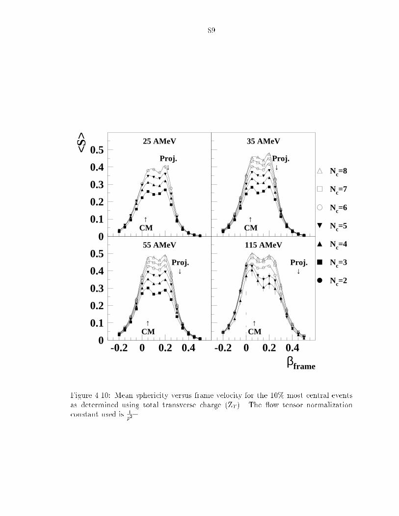
89
βframe
<S>
Nc=2
Nc=3
Nc=4
Nc=5
Nc=6
Nc=7
Nc=8
25 AMeV
Proj.↓
↑CM
35 AMeV
Proj.↓
↑CM
55 AMeV
Proj.↓
↑CM
115 AMeV
Proj.↓
CM↑
0
0.1
0.2
0.3
0.4
0.5
0
0.1
0.2
0.3
0.4
0.5
-0.2 0 0.2 0.4 -0.2 0 0.2 0.4
Figure 4.10: Mean sphericity versus frame velocity for the 10% most central events
as determined using total transverse charge (ZT ). The ow tensor normalizationconstant used is 1
p2.
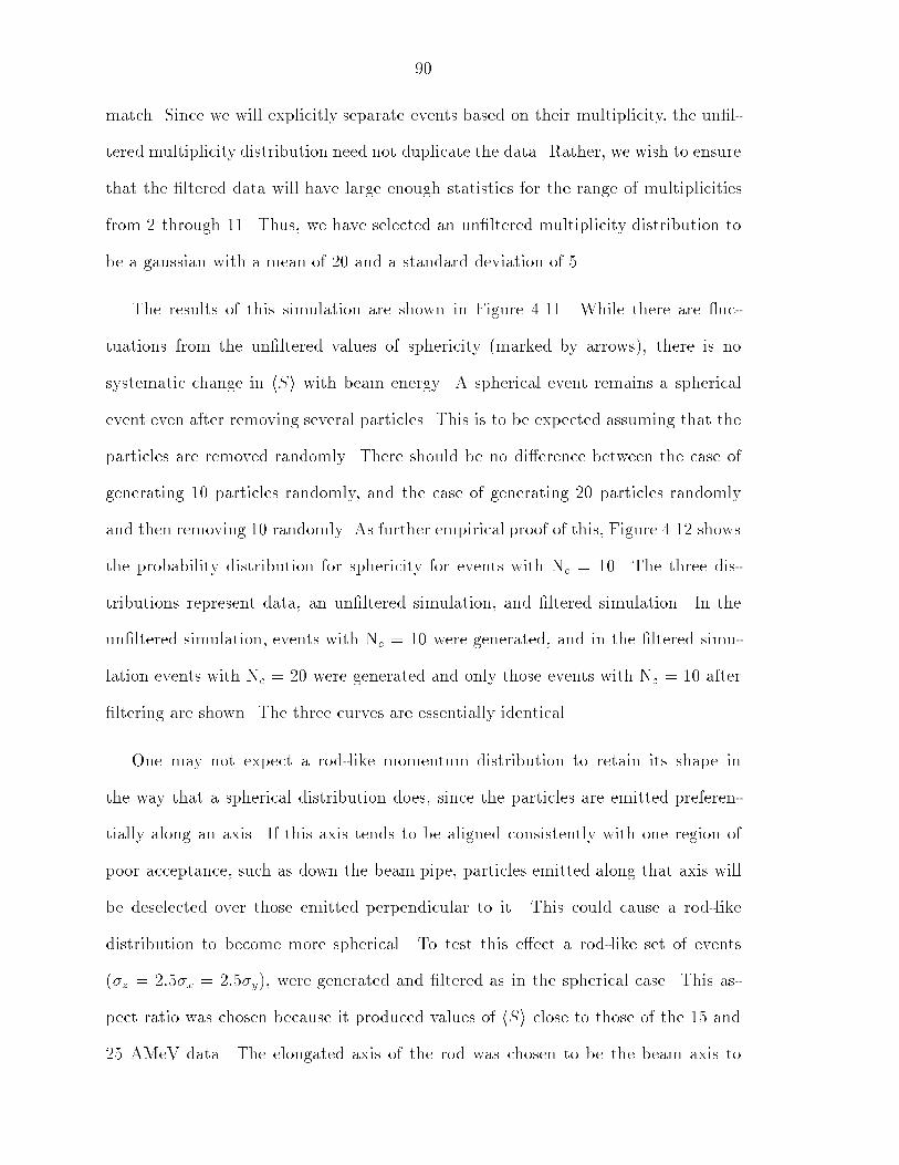
90
match. Since we will explicitly separate events based on their multiplicity, the un�l-
tered multiplicity distribution need not duplicate the data. Rather, we wish to ensure
that the �ltered data will have large enough statistics for the range of multiplicities
from 2 through 11. Thus, we have selected an un�ltered multiplicity distribution to
be a gaussian with a mean of 20 and a standard deviation of 5.
The results of this simulation are shown in Figure 4.11. While there are uc-
tuations from the un�ltered values of sphericity (marked by arrows), there is no
systematic change in hSi with beam energy. A spherical event remains a spherical
event even after removing several particles. This is to be expected assuming that the
particles are removed randomly. There should be no di�erence between the case of
generating 10 particles randomly, and the case of generating 20 particles randomly
and then removing 10 randomly. As further empirical proof of this, Figure 4.12 shows
the probability distribution for sphericity for events with Nc = 10. The three dis-
tributions represent data, an un�ltered simulation, and �ltered simulation. In the
un�ltered simulation, events with Nc = 10 were generated, and in the �ltered simu-
lation events with Nc = 20 were generated and only those events with Nc = 10 after
�ltering are shown. The three curves are essentially identical.
One may not expect a rod-like momentum distribution to retain its shape in
the way that a spherical distribution does, since the particles are emitted preferen-
tially along an axis. If this axis tends to be aligned consistently with one region of
poor acceptance, such as down the beam pipe, particles emitted along that axis will
be deselected over those emitted perpendicular to it. This could cause a rod-like
distribution to become more spherical. To test this e�ect a rod-like set of events
(�z = 2:5�x = 2:5�y), were generated and �ltered as in the spherical case. This as-
pect ratio was chosen because it produced values of hSi close to those of the 15 and25 AMeV data. The elongated axis of the rod was chosen to be the beam axis to
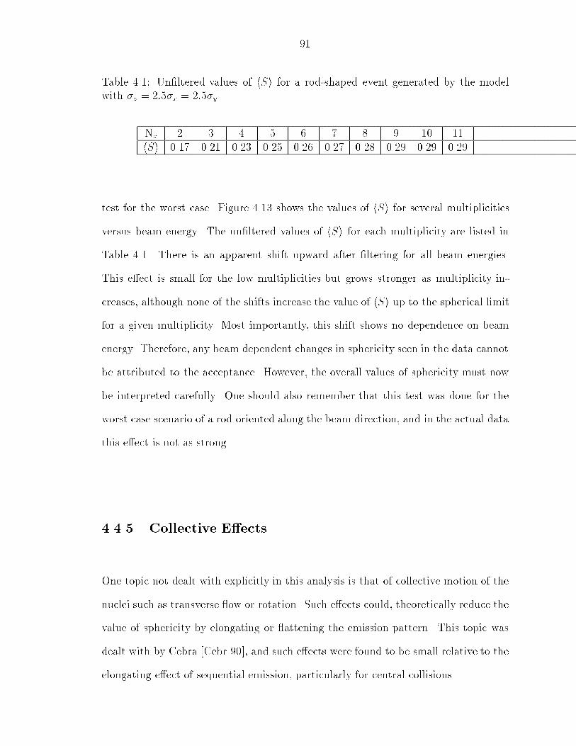
91
Table 4.1: Un�ltered values of hSi for a rod-shaped event generated by the modelwith �z = 2:5�x = 2:5�y.
Nc 2 3 4 5 6 7 8 9 10 11
hSi 0.17 0.21 0.23 0.25 0.26 0.27 0.28 0.29 0.29 0.29
test for the worst case. Figure 4.13 shows the values of hSi for several multiplicitiesversus beam energy. The un�ltered values of hSi for each multiplicity are listed in
Table 4.1. There is an apparent shift upward after �ltering for all beam energies.
This e�ect is small for the low multiplicities but grows stronger as multiplicity in-
creases, although none of the shifts increase the value of hSi up to the spherical limit
for a given multiplicity. Most importantly, this shift shows no dependence on beam
energy. Therefore, any beam dependent changes in sphericity seen in the data cannot
be attributed to the acceptance. However, the overall values of sphericity must now
be interpreted carefully. One should also remember that this test was done for the
worst case scenario of a rod oriented along the beam direction, and in the actual data
this e�ect is not as strong.
4.4.5 Collective E�ects
One topic not dealt with explicitly in this analysis is that of collective motion of the
nuclei such as transverse ow or rotation. Such e�ects could, theoretically reduce the
value of sphericity by elongating or attening the emission pattern. This topic was
dealt with by Cebra [Cebr 90], and such e�ects were found to be small relative to the
elongating e�ect of sequential emission, particularly for central collisions.
92
Ebeam [AMeV]
<S>
← Smax2
← Smax3
← Smax4
← Smax5
← Smax6
← Smax7
← Smax8
← Smax9
← Smax10
← Smax11
Nc=2
Nc=3
Nc=4
Nc=5
Nc=6
Nc=7
Nc=8
Nc=9
Nc=10
Nc=11
0.1
0.15
0.2
0.25
0.3
0.35
0.4
0.45
0.5
0.55
0.6
20 40 60 80 100 120
Figure 4.11: Mean sphericity versus beam energy for 9 event sets each generatedwith a spherical ow ellipsoid, and boosted to one of the center-of-mass velocities
corresponding to the 9 beam energies. The data was then �ltered through a software
replica of the 4� Array.
93
Sphericity
P(S
pher
icit
y)
Data
Simulation (Unfiltered)
Simulation (Filtered)
0
0.01
0.02
0.03
0.04
0.05
0.06
0.07
0 0.1 0.2 0.3 0.4 0.5 0.6 0.7 0.8 0.9 1
Figure 4.12: Sphericity probability distribution for events with multiplicity Nc = 10,
from experimental data, un�ltered simulation, and �ltered simulation. For the un�l-
tered simulation, all events were generated with Nc = 10. For the �ltered simulation,
events were generated with Nc = 20, and only those events with Nc = 10 after �ltering
are plotted.
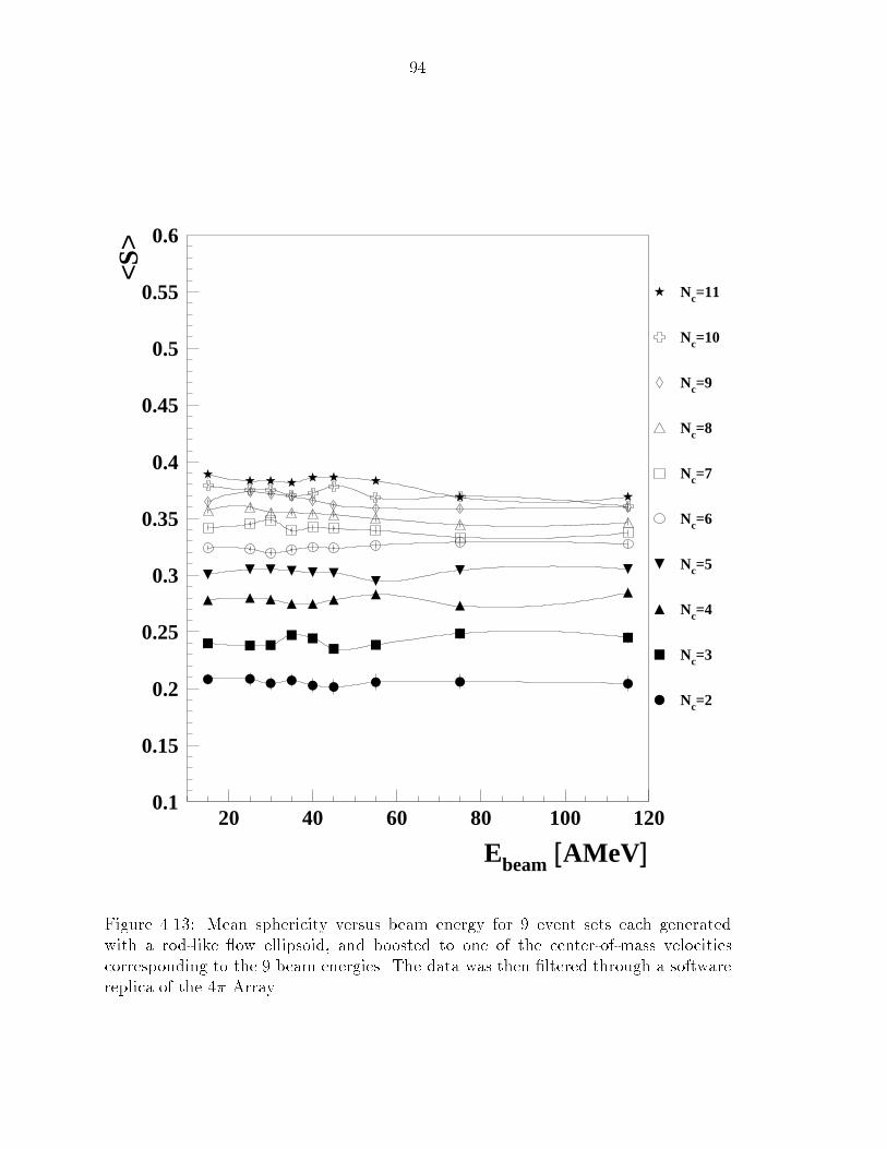
94
Ebeam [AMeV]
<S>
Nc=2
Nc=3
Nc=4
Nc=5
Nc=6
Nc=7
Nc=8
Nc=9
Nc=10
Nc=11
0.1
0.15
0.2
0.25
0.3
0.35
0.4
0.45
0.5
0.55
0.6
20 40 60 80 100 120
Figure 4.13: Mean sphericity versus beam energy for 9 event sets each generatedwith a rod-like ow ellipsoid, and boosted to one of the center-of-mass velocities
corresponding to the 9 beam energies. The data was then �ltered through a software
replica of the 4� Array.
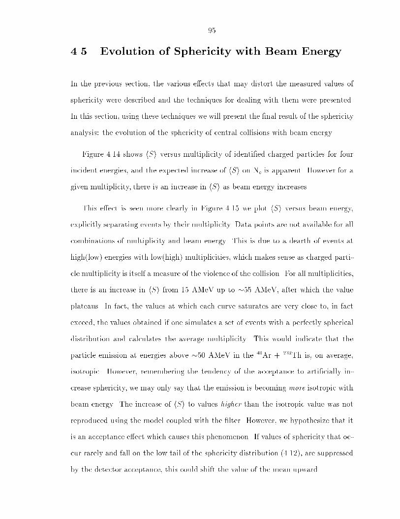
95
4.5 Evolution of Sphericity with Beam Energy
In the previous section, the various e�ects that may distort the measured values of
sphericity were described and the techniques for dealing with them were presented.
In this section, using these techniques we will present the �nal result of the sphericity
analysis: the evolution of the sphericity of central collisions with beam energy.
Figure 4.14 shows hSi versus multiplicity of identi�ed charged particles for four
incident energies, and the expected increase of hSi on Nc is apparent. However for a
given multiplicity, there is an increase in hSi as beam energy increases.
This e�ect is seen more clearly in Figure 4.15 we plot hSi versus beam energy,
explicitly separating events by their multiplicity. Data points are not available for all
combinations of multiplicity and beam energy. This is due to a dearth of events at
high(low) energies with low(high) multiplicities, which makes sense as charged parti-
cle multiplicity is itself a measure of the violence of the collision. For all multiplicities,
there is an increase in hSi from 15 AMeV up to �55 AMeV, after which the value
plateaus. In fact, the values at which each curve saturates are very close to, in fact
exceed, the values obtained if one simulates a set of events with a perfectly spherical
distribution and calculates the average multiplicity. This would indicate that the
particle emission at energies above �50 AMeV in the 40Ar + 232Th is, on average,
isotropic. However, remembering the tendency of the acceptance to arti�cially in-
crease sphericity, we may only say that the emission is becoming more isotropic with
beam energy. The increase of hSi to values higher than the isotropic value was not
reproduced using the model coupled with the �lter. However, we hypothesize that it
is an acceptance e�ect which causes this phenomenon. If values of sphericity that oc-
cur rarely and fall on the low tail of the sphericity distribution (4.12), are suppressed
by the detector acceptance, this could shift the value of the mean upward.
96
Nc
<S>
25 AMeV
35 AMeV
55 AMeV
115 AMeV
0.2
0.3
0.4
0.5
0.6
0 2 4 6 8 10 12 14
Figure 4.14: Mean values of sphericity plotted versus charged particle multiplicity(Nc), for four incident beam energies of 40Ar + 232Th. The data is for central collisions.
97
Thus far, we have only included fully identi�ed particles in the sphericity analysis.
That is, we have excluded �ssion fragments since we do not have easy experimental
access to their energy. However, in using the 1p2
normalization, the energy of the
particles is not needed explicitly in the ow tensor. Only the angles of emission are
needed, and these are very well known for the �ssion fragments due to the excellent
angular resolution of the MWPCs. However, the velocity of the fragments is needed
in order to correctly transform the angles them to the center of mass frame. The ve-
locity can be estimated quite accurately using the Viola prescription [Poll 84, Viol 85]
described in the previous chapter. The results of including the �ssion fragments in
the sphericity calculation are shown in Figure 4.16. This plot is very similar to the
preceding one except for two features. First, since we have added particles, the statis-
tics are improved and we are able to include data points for energy and multiplicity
combinations not possible without including the �ssion fragments. Second, the values
of hSi are slightly suppressed at the lower energies. This latter point makes sense as
we are adding particles that are emitted along, in fact de�ne, a particular axis, and
would tend to elongate the shape of the particle ow ellipsoid.
For completeness, we include a plot of hSi versus beam energy using the 12m
nor-
malization, for the same set of central events used in the preceding two plots. In
Figure 4.17, the same upward trend is seen in the curves from 15 AMeV, up to 55
AMeV. However, beyond that point the curves fall back down again. This is a veri�-
cation that the faster source has a large in uence on the value of sphericity calculated
in the center-of-mass frame, and justi�es our choice of the 1p2
normalization. As the
projectile velocity grows increasingly larger than the center-of-mass velocity, the value
of hSi becomes increasingly suppressed. Since switching to the 1p2
normalization in-
creases the values of hSi at the highest energies relative to those at the lower energies,we conclude that the e�ect of the faster source is relatively small at the lower energies.
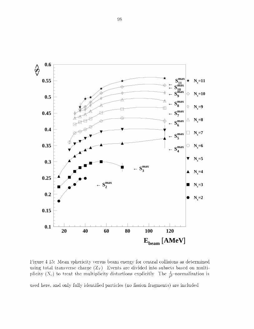
98
Ebeam [AMeV]
<S>
← Smax2
← Smax3
← Smax4
← Smax5
← Smax6
← Smax7
← Smax8
← Smax9
← Smax10
← Smax11
Nc=2
Nc=3
Nc=4
Nc=5
Nc=6
Nc=7
Nc=8
Nc=9
Nc=10
Nc=11
0.1
0.15
0.2
0.25
0.3
0.35
0.4
0.45
0.5
0.55
0.6
20 40 60 80 100 120
Figure 4.15: Mean sphericity versus beam energy for central collisions as determined
using total transverse charge (ZT ). Events are divided into subsets based on multi-
plicity (Nc) to treat the multiplicity distortions explicitly. The 1p2
normalization is
used here, and only fully identi�ed particles (no �ssion fragments) are included.
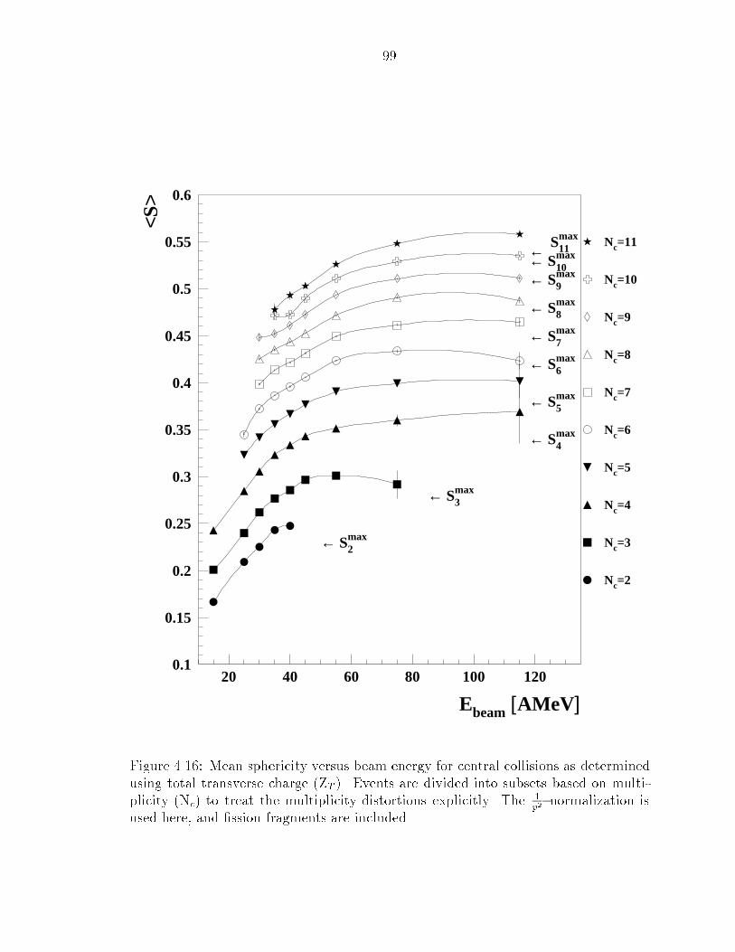
99
Ebeam [AMeV]
<S>
← Smax2
← Smax3
← Smax4
← Smax5
← Smax6
← Smax7
← Smax8
← Smax9
← Smax10
← Smax11
Nc=2
Nc=3
Nc=4
Nc=5
Nc=6
Nc=7
Nc=8
Nc=9
Nc=10
Nc=11
0.1
0.15
0.2
0.25
0.3
0.35
0.4
0.45
0.5
0.55
0.6
20 40 60 80 100 120
Figure 4.16: Mean sphericity versus beam energy for central collisions as determinedusing total transverse charge (ZT ). Events are divided into subsets based on multi-
plicity (Nc) to treat the multiplicity distortions explicitly. The 1p2
normalization is
used here, and �ssion fragments are included.
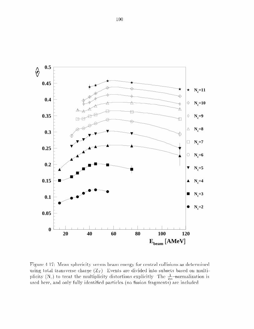
100
Ebeam [AMeV]
<S>
Nc=2
Nc=3
Nc=4
Nc=5
Nc=6
Nc=7
Nc=8
Nc=9
Nc=10
Nc=11
0
0.05
0.1
0.15
0.2
0.25
0.3
0.35
0.4
0.45
0.5
20 40 60 80 100 120
Figure 4.17: Mean sphericity versus beam energy for central collisions as determined
using total transverse charge (ZT ). Events are divided into subsets based on multi-
plicity (Nc) to treat the multiplicity distortions explicitly. The 12m
normalization isused here, and only fully identi�ed particles (no �ssion fragments) are included.
101
4.6 Summary and Discussion
In this chapter we have shown that there is a signi�cant increase in the average spheric-
ity of central collisions of 40Ar + 232Th as bombarding energy increases. For energies
above �50 AMeV, the measured value of hSi is close to the value obtained from an
isotropic distribution. This increase is similar to what has been seen previously in
studies of symmetric systems [Cebr 90, Cebr 90a, Barz 91]. It has been suggested
through various model calculations that sphericity is expected to be higher for the si-
multaneous breakup of a system than for sequential breakup through a series of binary
decays, and may approach isotropy [Lope 89, Cebr 90, Cebr 90a, Harm 90, Barz 91].
We interpret our results as signifying a gradual change in the dominant reaction mech-
anism from a sequential binary decay (e.g fusion-�ssion) to a more prompt scenario
(e.g. multifragmentation). However, due to acceptance e�ects which cause an overall
upward shift in hSi for all beam energies, we can only place a lower limit on the
bombarding energy at which we believe the prompt mechanism becomes dominant.
We report this bombarding energy to be 50 AMeV.

102
Chapter 5
Conclusion
To study the evolution of the reaction mechanism in central collisions of heavy ions
on �ssionable targets, we studied the 40Ar + 232Th system at bombarding energies
ranging from 15 - 115 AMeV using the MSU 4� Array. At the time of the experiment,
the Array consisted of the 30, recently completed, multi-wire proportional counters
for the detection of �ssion fragments, backed by 55 Bragg Curve Counters for the
detection of intermediate mass fragments, and �nally backed by 170 high dynamic
range fast/slow plastic phoswiches for the detection of particles with charges from Z=
1-8. An additional array of 45 plastic phoswiches covered forward angles.
Disappearance of Fusion-�ssion
While the fusion-�ssion process was found to decline steadily in central collisions as
bombarding energy is increased, in agreement with previous measurements, evidence
of a �ssion-like reaction mechanism has been found in the 40Ar + 232Th system in
the most central collisions at all bombarding energies studied, including 115 AMeV.
That this process is seen at this energy suggests that nuclei are indeed capable of
containing large amounts of excitation energy long enough for an inherently slow
collective process, such as �ssion, to occur. However, the probability for this scenario
103
104
to occur becomes increasingly unlikely as excitation energies are increased up through
� 1 GeV.
Momentum Transfer and Excitation Energy
Average momentum transfer has been measured for the impact parameter inclusive
�ssion event set in this system, and the most probable momentum transfer has been
measured for the most central events leading to �ssion. The most probable momentum
transfer, as a fraction of beam momentum, is found to follow known systematics as
beam velocity is increased [Viol 82, Nife 85], including the two highest energies for
which this observable was not previously available for this system. The average
momentum transfer was found to fall below the values predicted by the systematics
as beam energy increases and the �ssion channel is fed increasingly by peripheral
collisions. The most probable momentum transfer per projectile nucleon saturates
at �170 MeV/c for bombarding energies above 25 AMeV. This is in agreement with
previous experimental results [Tsan 84, Conj 85], and provides further evidence that
momenta above the Fermi momentum are not easily imparted to a compound system
[Woo 83, Sain 84].
Trends in average IMF and LCP production indicate that increasing amounts of
energy are being deposited in the 40Ar + 232Th system as beam energy increases. A
calculation of excitation energy based on an empirical relationship with momentum
transfer also indicates that excitation energy is increasing, and agrees well with the
values predicted by a schematic, hydrodynamic model [Harp 71, Desb 87, Cerr 89].
105
Event Shape Analysis
An analysis of the evolution of the event shape shows an increase in the average
sphericity of the most central events as beam energy increases. This increase is most
rapid in the 15 - 45 AMeV range and then saturates near the the value corresponding
to an isotropic distribution. This can be interpreted as a transition in the dominant
reaction mechanism from a sequential binary decay to a simultaneous one [Lope 89,
Cebr 90a]. However, due to acceptance e�ects which can shift the measured value of
sphericity uniformly upward for all energies studied, we can only put a lower limit
on the beam energy at which this transition might be complete. This energy is 55
AMeV.

106
Appendix A
Impact Parameter Filters
A.1 Method
In many experiments, including the present one, it is desirable to make exclusive
measurements of the properties of central collisions. One of the most powerful ad-
vantages of a 4� device is its ability to act as an impact parameter �lter and aid in
these measurements. Impact parameter is not directly accessible experimentally, but
there are several \centrality" variables which have been shown to be correlated with
impact parameter [Cava 90, Phai 92], and which the MSU 4� Array can determine
rather well. These variables include total charged particle multiplicity (Nc), midra-
pidity charge (Zmr), total transverse kinetic energy (ET ), and total transverse charge
(ZT ).
Total transverse kinetic energy is de�ned as the sum over the transverse kinetic
energy of each particle in an event:
ET =Xi
Eisin2�i =
Xi
(pisin�i)2=2mi: (A:1)
Similarly total transverse charge is de�ned as the sum over the charge of each particle
in the event, weighted by its polar angle:
ZT =Xi
Zisin�i: (A:2)
107
108
Midrapidity charge is the sum over the charge of all particles having a rapidity in the
center-of-mass which is greater that 75% of the center-of-mass target rapidity (y')
and less than 75% of the center-of-mass projectile rapidity, i.e.:
0:75y0targ
� y0 � 0:75y0
proj: (A:3)
The lab rapidity , y, of a particle is de�ned as
y =1
2lnf(
qm2 + p2 + pcos�)=(
qm2 + p2 � pcos�)g = tanh
�1(�cos�; ) (A:4)
where m, �, and p denote the particle's mass, velocity, and momentum, respectively.
To obtain a quantitative estimate of impact parameter from these variables, we use
the geometrical prescription of Reference [Cava 90]. It is assumed that each variable
(q) is monotonically related to impact parameter (b) and the following relation can
be written:
2�bdb
�b2max
= �f(q)dq; (A:5)
where bmax is the maximum impact parameter of the reaction and f(q) is the proba-
bility density function of q. That is, f(q)dq is the probability of detecting a collision
with a value of q' between q and q+ dq. The function f(q) is normalized to unity;
the plus/minus signs indicate that the variable q increases/decreases as b increases.
Integrating Equation A.5 from b to bmax we obtain:
Zbmax
b
2bdb
b2max
= �Z
q(bmax)
q(b)f(q0)dq0: (A:6)
If we let
F (q) = �Z
q(bmax)
q(b)f(q0)dq0; (A:7)
then
b=bmax =q1 � F (q): (A:8)

109
Using Equation A.8 one can easily make an estimate of impact parameter. The
experimental distribution of the centrality variable, q is integrated, and the value
of q corresponding to the desired value of b/bmax is determined. This value is then
used as a threshold to accept or reject events. In the present data, q was chosen
such that the largest values of b allowed are � 0:31bmax. This corresponds to � 10%
of the measured cross section. If the measured cross section were assumed to be
equivalent to the geometric (hard sphere) cross section, then bmax would be the sum
of the target and projectile radii (Rp + Rt). However, due to trigger bias and detector
acceptance, the actual impact parameter leading to a triggering event is less than (Rp
+ Rt) [Llop 95]. Thus, we can consider 0.31(Rp + Rt) to be an upper limit for our
maximum impact parameter.
A.2 Choice of Centrality Variable
In order to decide which of these variables to use, one must determine which is most
e�cient at selecting central collisions for the system under study. One must also
check the degree to which the observables of interest autocorrelate with the chosen
centrality variable [Conr 93, Llop 95].
A.2.1 Correlation with Folding Angle
In Chapter 3, the correlation between impact parameter and �ssion fragment folding
angle was discussed. It was explained that central, high LMT events lead to folding
angles of �100o - 110o, and peripheral, low LMT collisions give folding angles of
�160o - 170o , for this system. In Figures A.1-A.4, the four centrality variables are
plotted versus folding angle (�ff ). While there is a general correlation between all of
the centrality variables and the folding angle which grows stronger as beam energy
increases, the degree of this correlation is not the same for all of the variables.
110
Figure A.5 shows this e�ect more dramatically. In this plot, the folding angle
distributions from central collisions as de�ned by the various centrality variables
mentioned above, are shown. All of the variables suppress the target �ssion peak,
relative to the high LMT peak (compare Figure 3.2). However, at the low energies
there are some qualitative di�erences. We can state that ET and ZT are superior at
suppressing the peripheral component and are the preferred choices.
A.2.2 Sphericity as a Test of a Centrality Variable's E�-
ciency
Sphericity can also be used to test a centrality variables ability to suppress peripheral
collisions. As stated in Chapter 4, sphericity is maximum when it is calculated in
the frame of the emitting source. Thus, if there is more than one source velocity,
there should be more than one frame in which sphericity reaches a (local) maximum.
This was shown to be true in Chapter 4 as there were two bumps in the hSi vs.�frame curves for central events chosen with ZT , one near the center-of-mass velocity
and one at much faster velocities. By plotting hSi versus �frame for central collisions
selected with di�erent variables, we can roughly compare the relative size of this
faster, projectile-like contribution. We can also compare the positions of the center-
of-mass peaks, assuming that this peak will be shifted to faster velocities if there is a
stronger contribution from peripheral collisions.
As Figures A.6 and A.7 show, ZT seems to do a better job suppressing the
projectile-like source. The size of this contribution is smaller, and the peak is lo-
cated at slower velocities than when ET is used. Thus we can say that ZT is our �rst
choice as a centrality variable, with ET also being acceptable.
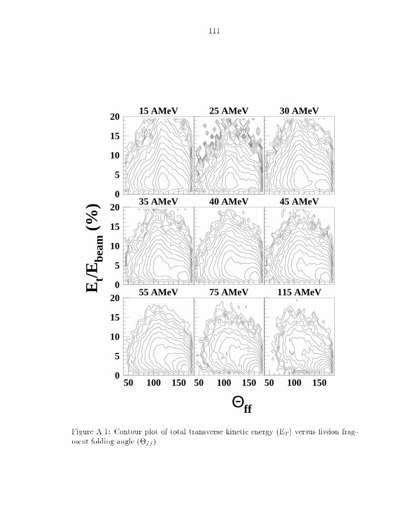
111
Θff
Et/E
beam
(%
)
15 AMeV 25 AMeV 30 AMeV
35 AMeV 40 AMeV 45 AMeV
55 AMeV 75 AMeV 115 AMeV
0
5
10
15
20
0
5
10
15
20
0
5
10
15
20
50 100 150 50 100 150 50 100 150
Figure A.1: Contour plot of total transverse kinetic energy (ET ) versus �ssion frag-
ment folding angle (�ff).
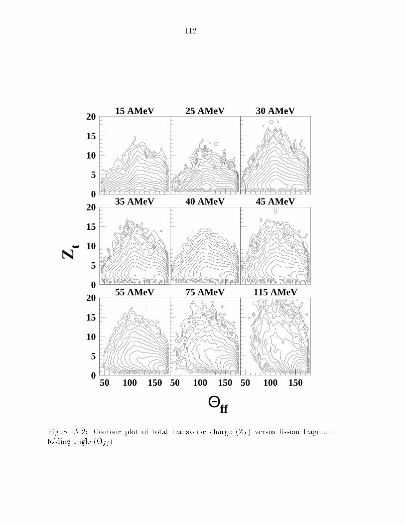
112
Θff
Zt
15 AMeV 25 AMeV 30 AMeV
35 AMeV 40 AMeV 45 AMeV
55 AMeV 75 AMeV 115 AMeV
0
5
10
15
20
0
5
10
15
20
0
5
10
15
20
50 100 150 50 100 150 50 100 150
Figure A.2: Contour plot of total transverse charge (ZT ) versus �ssion fragment
folding angle (�ff).
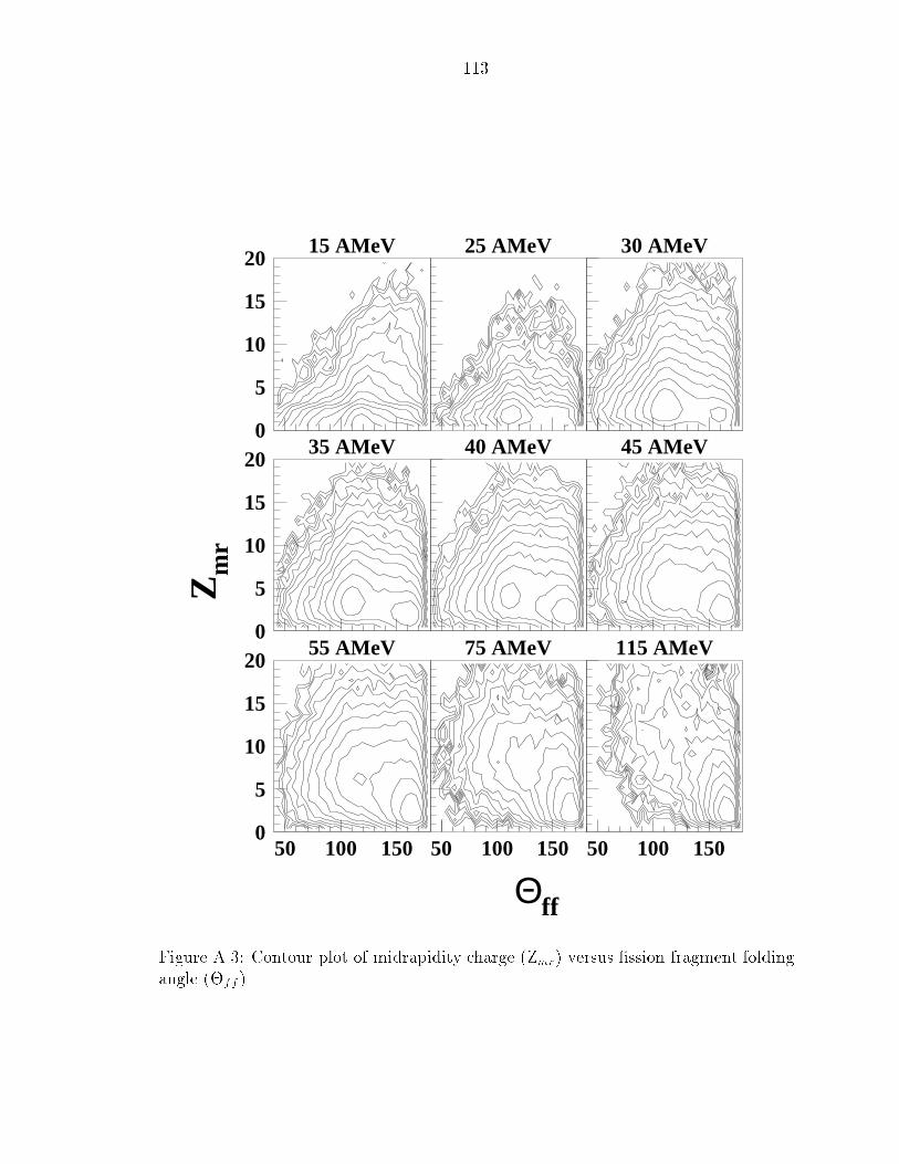
113
Θff
Zm
r
15 AMeV 25 AMeV 30 AMeV
35 AMeV 40 AMeV 45 AMeV
55 AMeV 75 AMeV 115 AMeV
0
5
10
15
20
0
5
10
15
20
0
5
10
15
20
50 100 150 50 100 150 50 100 150
Figure A.3: Contour plot of midrapidity charge (Zmr) versus �ssion fragment folding
angle (�ff ).
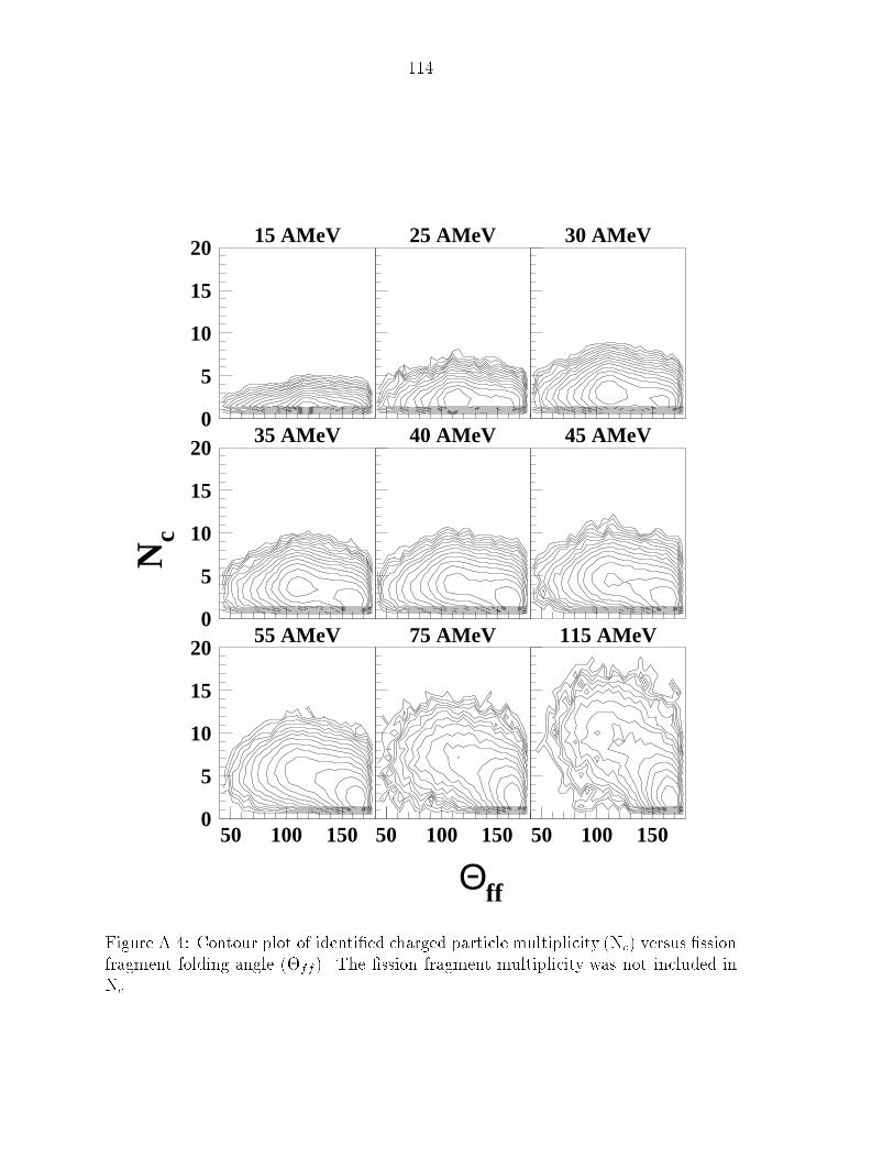
114
Θff
Nc
15 AMeV 25 AMeV 30 AMeV
35 AMeV 40 AMeV 45 AMeV
55 AMeV 75 AMeV 115 AMeV
0
5
10
15
20
0
5
10
15
20
0
5
10
15
20
50 100 150 50 100 150 50 100 150
Figure A.4: Contour plot of identi�ed charged particle multiplicity (Nc) versus �ssion
fragment folding angle (�ff). The �ssion fragment multiplicity was not included in
Nc.
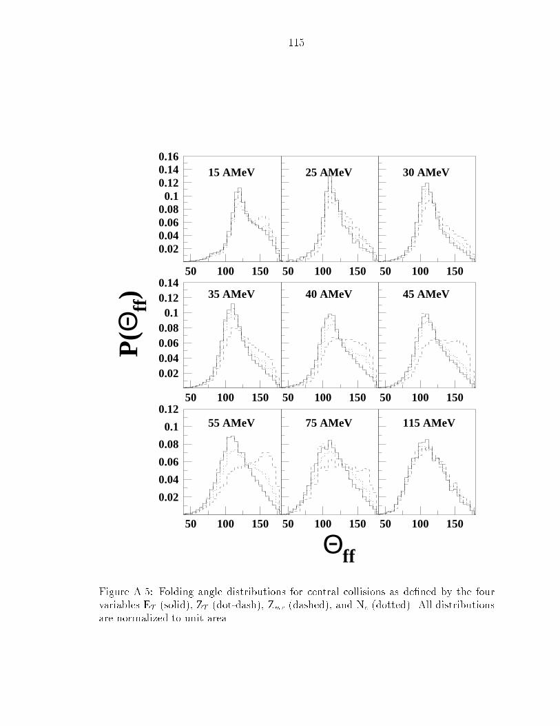
115
Θff
P(Θ
ff)
15 AMeV 25 AMeV 30 AMeV
35 AMeV 40 AMeV 45 AMeV
55 AMeV 75 AMeV 115 AMeV
0.020.040.060.080.1
0.120.140.16
50 100 150 50 100 150 50 100 150
0.020.040.060.080.1
0.120.14
50 100 150 50 100 150 50 100 150
0.02
0.04
0.06
0.08
0.1
0.12
50 100 150 50 100 150 50 100 150
Figure A.5: Folding angle distributions for central collisions as de�ned by the fourvariables ET (solid), ZT (dot-dash), Zmr (dashed), and Nc (dotted). All distributions
are normalized to unit area.
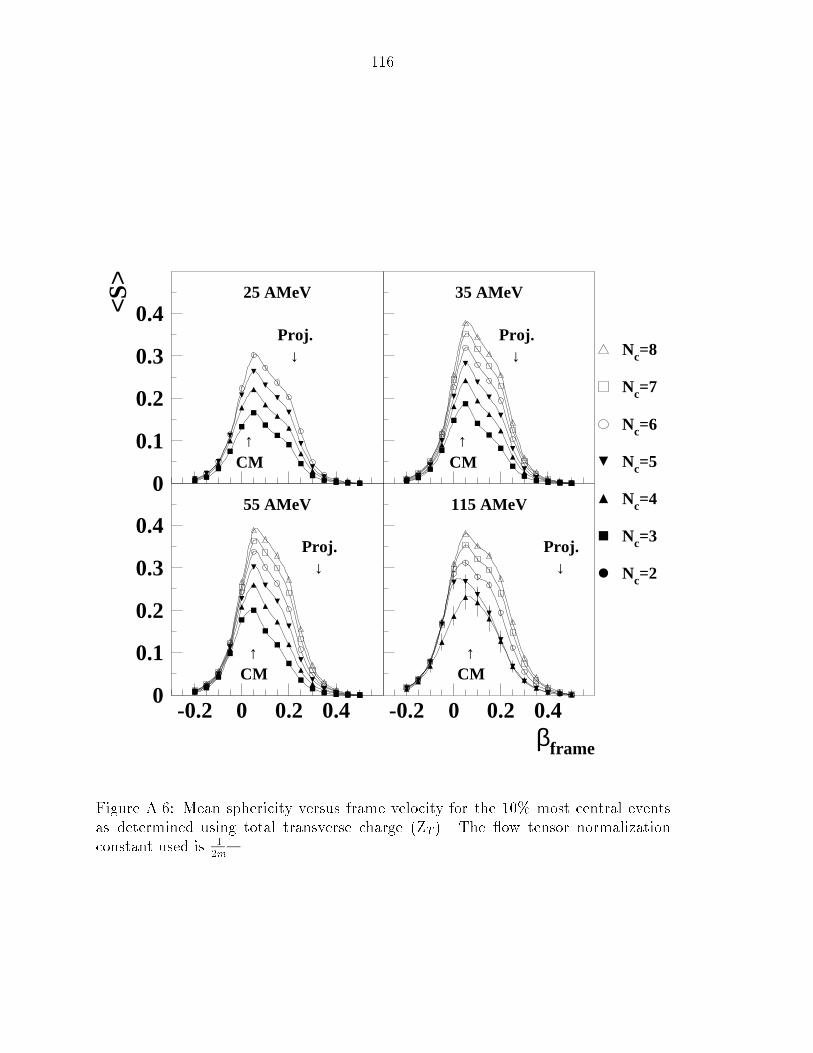
116
βframe
<S>
Nc=2
Nc=3
Nc=4
Nc=5
Nc=6
Nc=7
Nc=8
25 AMeV
Proj.↓
↑CM
35 AMeV
Proj.↓
↑CM
55 AMeV
Proj.↓
↑CM
115 AMeV
Proj.↓
CM↑
0
0.1
0.2
0.3
0.4
0
0.1
0.2
0.3
0.4
-0.2 0 0.2 0.4 -0.2 0 0.2 0.4
Figure A.6: Mean sphericity versus frame velocity for the 10% most central eventsas determined using total transverse charge (ZT ). The ow tensor normalization
constant used is 12m.
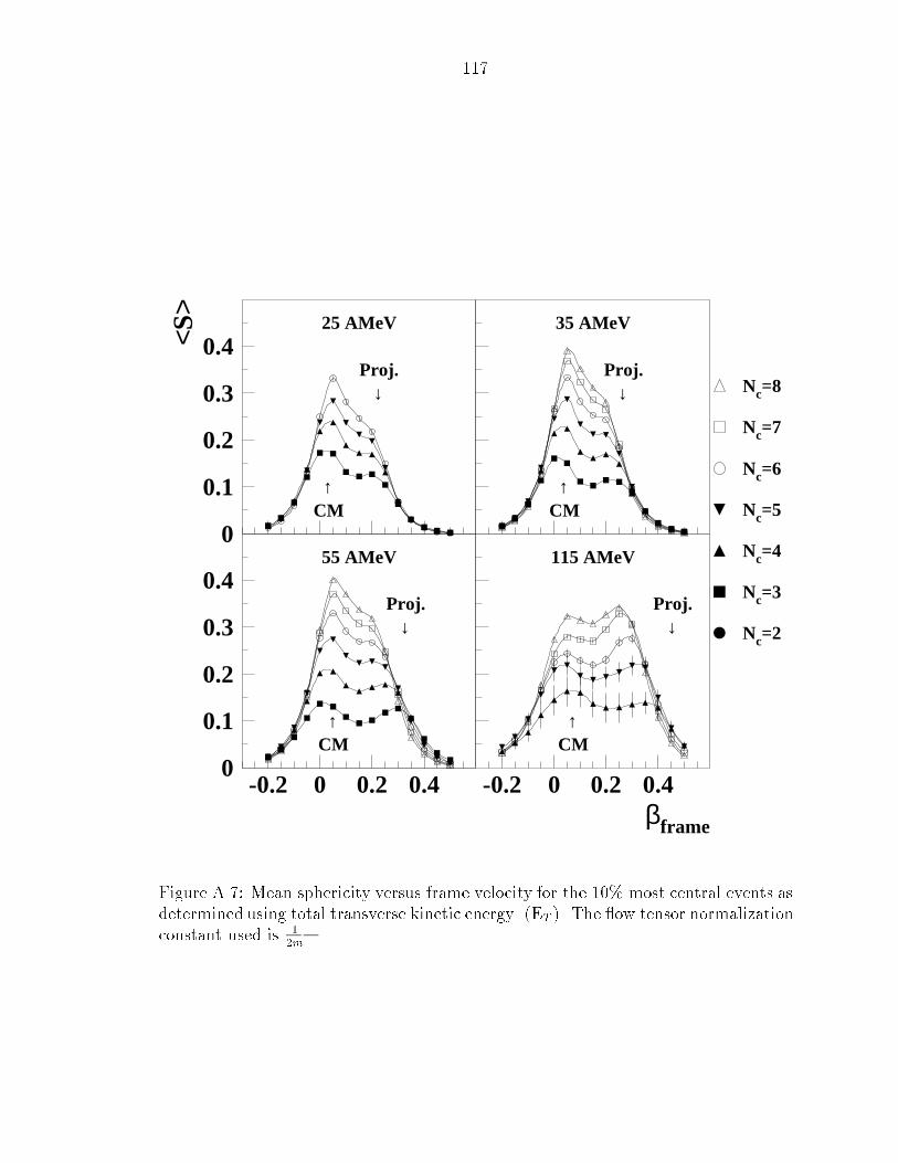
117
βframe
<S>
Nc=2
Nc=3
Nc=4
Nc=5
Nc=6
Nc=7
Nc=8
25 AMeV
Proj.↓
↑CM
35 AMeV
Proj.↓
↑CM
55 AMeV
Proj.↓
↑CM
115 AMeV
Proj.↓
CM↑
0
0.1
0.2
0.3
0.4
0
0.1
0.2
0.3
0.4
-0.2 0 0.2 0.4 -0.2 0 0.2 0.4
Figure A.7: Mean sphericity versus frame velocity for the 10% most central events asdetermined using total transverse kinetic energy. (ET ). The ow tensor normalization
constant used is 12m.
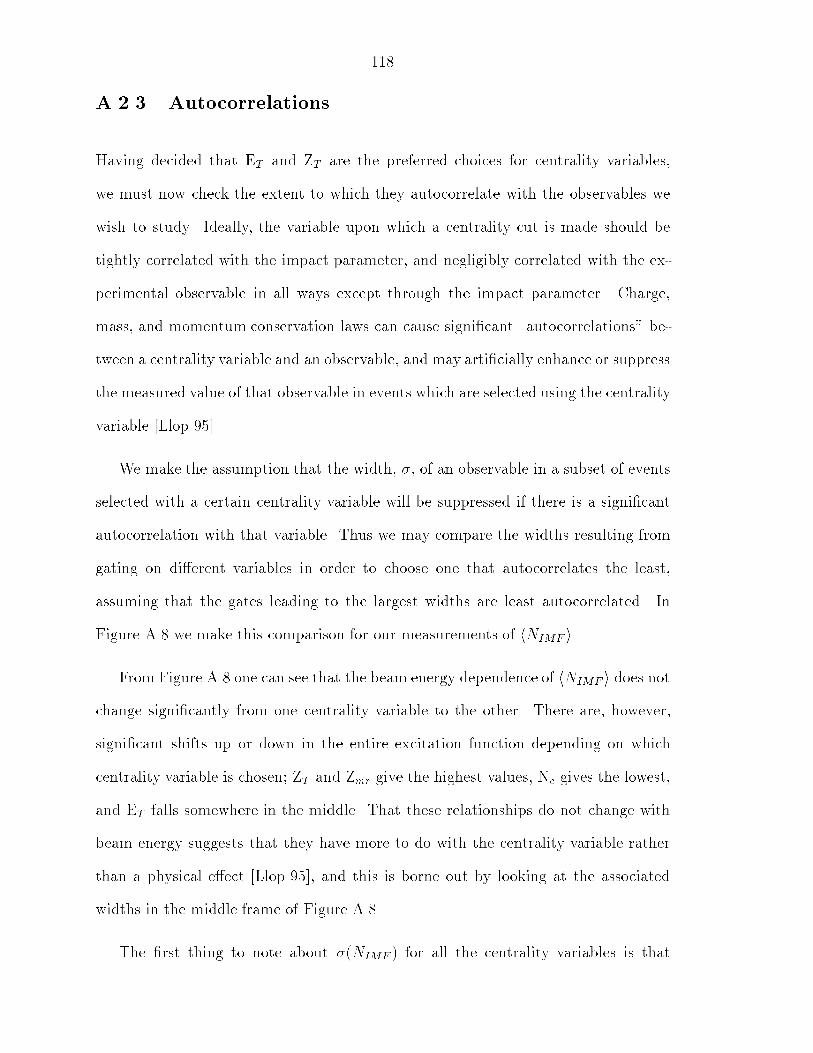
118
A.2.3 Autocorrelations
Having decided that ET and ZT are the preferred choices for centrality variables,
we must now check the extent to which they autocorrelate with the observables we
wish to study. Ideally, the variable upon which a centrality cut is made should be
tightly correlated with the impact parameter, and negligibly correlated with the ex-
perimental observable in all ways except through the impact parameter. Charge,
mass, and momentum conservation laws can cause signi�cant \autocorrelations" be-
tween a centrality variable and an observable, and may arti�cially enhance or suppress
the measured value of that observable in events which are selected using the centrality
variable [Llop 95].
We make the assumption that the width, �, of an observable in a subset of events
selected with a certain centrality variable will be suppressed if there is a signi�cant
autocorrelation with that variable. Thus we may compare the widths resulting from
gating on di�erent variables in order to choose one that autocorrelates the least,
assuming that the gates leading to the largest widths are least autocorrelated. In
Figure A.8 we make this comparison for our measurements of hNIMF i.
From Figure A.8 one can see that the beam energy dependence of hNIMF i does notchange signi�cantly from one centrality variable to the other. There are, however,
signi�cant shifts up or down in the entire excitation function depending on which
centrality variable is chosen; ZT and Zmr give the highest values, Nc gives the lowest,
and ET falls somewhere in the middle. That these relationships do not change with
beam energy suggests that they have more to do with the centrality variable rather
than a physical e�ect [Llop 95], and this is borne out by looking at the associated
widths in the middle frame of Figure A.8.
The �rst thing to note about �(NIMF ) for all the centrality variables is that
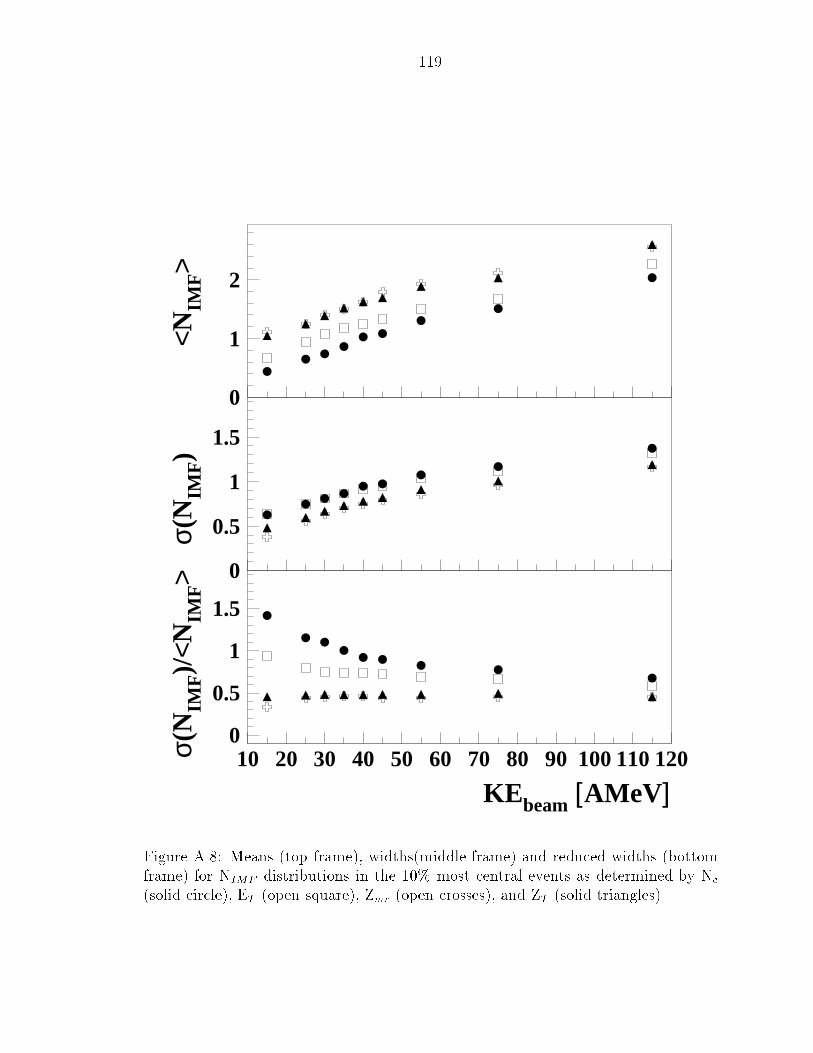
119
<NIM
F>
σ(N
IMF)
KEbeam [AMeV]
σ(N
IMF)/
<NIM
F>
0
1
2
0
0.5
1
1.5
0
0.5
1
1.5
10 20 30 40 50 60 70 80 90 100 110 120
Figure A.8: Means (top frame), widths(middle frame) and reduced widths (bottom
frame) for NIMF distributions in the 10% most central events as determined by Nc
(solid circle), ET (open square), Zmr (open crosses), and ZT (solid triangles).
120
they are quite large relative to hNIMF i. However, two distinct groups are evident:
one containing Zmr and ZT , and one containing ET and Nc. The widths resulting
from the Zmr and ZT cuts are smaller than those resulting from the ET and Nc cuts,
indicating that the former variables autocorrelate more strongly than latter ones, and
should be avoided. This result agrees with that of Reference [Llop 95].
The bottom frame of Figure A.8 shows that the reduced widths, �(NIMF )
hNIMF i , for the
ET and Nc selected events are similar for the highest three energies, but di�er greatly
at the lower energies with�(NIMF )
hNIMF i being much higher for Nc. This can be explained
by what we have already shown in Section A.2.1: Nc is not a sensitive indicator of
central events at low energies, most likely due to the relatively low numbers of charged
particles produced in these collisions. Thus, we are left with ET as an appropriate
variable to use in our studies of hNIMF i.
A similar study has been done by Llope et al. [Llop 93] to test the autocorrelation
of sphericity with six di�erent centrality variables including most of those presented
here. This study included data from �ve symmetric systems ranging in size from C
+ C to Xe + La, and beam energies ranging from 15 AMeV to 155 AMeV. It was
found that for cuts on the order of 10%, such as those used in this analysis, there
are no signi�cant autocorrelations for any of the centrality variables. We make the
assumption that the same is true in this data, and choose ZT as our centrality variable
for sphericity studies based on the arguments of Section A.2.2.
Bibliography
[Awes 81] T.C. Awes, G. Poggi, C.K. Gelbke, B.B. Back, B.G. Glagola, H. Breuer,and V.E.Viola, Jr., Phys. Rev. C24, 89 (1981).
[Back 80] B.B. Back, K.L. Wolf, A.C. Mignerey, C.K. Gelbke, T.C. Awes, H. Breuer,V.E. Viola, Jr., P. Dyer, Phys. Rev. C22, 1927 (1980).
[Barz 91] H.W. Barz, D.A. Cebra, H. Schulz, G.D. Westfall, Phys. Lett. B267, 317(1991).
[Bege 92] M. Begemann-Blaich, Th. Blaich, M.M.Fowler, J.B. Wilhelmy, H.C. Britt,D.J. Fields, L.F Hansen, R.G. Lanier, D.J. Massoletti, M.N. Bamboodiri,B.A. Remington, T.C. Sangster, G.L. Struble, M.L. Webb, Y.D. Chan, A.Dacal, A. Harmon, J. Pouliot, R.G. Stokstad, S. Kaufman, F. Videbaek,Z.Fraenkel, Phys. Rev. C45, 677 (1992).
[Bhat 89] S. Bhattacharya, J.N. De, K. Krishan, S.K. Samaddar, Phys. Rev. Lett.62, 2589, (1989).
[Biza 93] G. Bizard, R. Bougault, R. Brou, J. Colin, D. Durand, A. Genoux-Lubain,J.L. laville, C. Le Brun, J.F. Lecolley, M. Louvel, J. P�eter, J.C. Steckmeyer,B. Tamain, A. Badala, T. Motobayashi, G. Rudolf, L. Stuttg�e, Phys. Lett.B302, 162 (1992).
[Bowm 91] D.R. Bowman, G.F. Peaslee, R.T. de Souza, N. Carlin, C.K. Gelbke,W.G. Gong, Y.D. Kim, M.A. Lisa, W.G. Lynch, L. Phair, M.B. Tsang,C. Williams, N. Colonna, K. Hanold, M.A. McMahan, G.J. Wozniak, L.G.Moretto, W.A. Friedman, Phys. Rev. Lett. 67, 1527 (1991).
[Blai 92] Th. Blaich, M. Begemann-Blaich, M.M. Fowler, J.B. Wilhelmy, H.C. Britt,D.J. Fields, L.F. Hansen, M.N. Namboodiri, T.C. Sangster, Z. Fraenkel,Phys. Rev. C45, 689 (1992).
[Bond 90] J.P. Bondorf et al., Phys. Lett 150B, 57 (1985).
[Bond 90a] J.P. Bondorf, C.H. Dasso, R. Donangelo, and G. Pollarolo, Phys. Lett.240B, 28 (1990).
[Camp 84] X. Campi, J. Desbois, E. Lipparini, Phys. Lett. B142, 8 (1984).
[Cava 90] C. Cavata, M. Demoulins, J. Gosset, M.-C. Lemaire, D. L'Hote, J. Poitou,O. Valette, Phys. Rev. C42, 1760 (1990).
121
122
[Cebr 90] D.A. Cebra, Ph.D. Thesis, Michigan State University,1990.
[Cebr 90a] D.A. Cebra, S. Howden, J. Karn, A. Nadasen, C.A. Ogilvie, A. VanderMolen, G.D. Westfall, W.K. Wilson, J.S. Win�eld, and E. Norbeck, Phys.Rev. Lett. 64, 2246 (1990).
[Cebr 91] D.A. Cebra, S. Howden, J. Karn, D. Kataria, M. Maier, A. Nadasen, E.Norbeck, C.A. Ogilvie, N. Stone, D. Swan, A. Vander Molen, W.K. Wilson,J.S. Win�eld, J. Yurkon and G.D. Westfall, Nucl. Inst. and Meth A300,518 (1991).
[Cerr 89] C.Cerruti, R. Boisgard, C. Ngo, and J. Desbois, Nucl. Phys. A492, 322(1989).
[Conj 85] M. Conjeaud, S. Harar, M. Mostefai, E.C. Pollacco, C. Volant, Y. Cassag-nou, R. Dayras, R. Legrain, H. Oeschler, and F. Saint-Laurent, Phys. Lett.159B, 244 (1985).
[Conr 93] J.A. Conrad, M.S. Thesis, Michigan State University, 1993.
[Cugn 82] J. Cugnon, J. Knoll, C. Riedel, and Y. Yariv, Phys. Lett. 109B, 167 (1982).
[Cugn 83] J. Cugnon and D. L'Hote, Nucl. Phys. A397, 519 (1983).
[Dani 83] P. Danielewicz and M. Gyulassy, Phys. Lett 129B, 283 (1983).
[Desb 87] J. Desbois, R. Boisgard, C. Ngo, and J. Nemeth, Z. Phys. A328, 101(1987).
[deSo 91] R.T. de Souza, L. Phair, D.R. Bowman, N. Carlin, C.K. Gelbke, W.G.Gong, Y.D. Kim, M.A. Lisa, W.G. Lynch, G.F. Peaslee, M.B. Tsang, H.M.Xu, F. Zhu, W.A. Friedman, Phys. Lett. B268, 6 (1991).
[Ethv 91] T. Ethvignot, A. Elmaani, N.N. Ajitanand, J.M. Alexander, E. Bauge, P.Bier, L. Kowalski, M.T. Magda, P. D�esesquelles, H. Elhage, A. Giorni, D.Heuer, S. Kox, A. Lleres, F. Merchez, C. Morand, D. Rebreyend, P. Stassi,J.B. Viano, S. Benrachi, B. Chambon, B. Cheynis, D. Drain, C. Pastor,Phys. Rev. C43, R2035 (1991).
[Fai 83] G. Fai and J. Randrup, Nucl. Phys. A404, 551 (1983).
[Faty 85] M. Fatyga, K. Kwiatkowski, V.E. Viola, C.B. Chitwood, D.J. Fields, C.K.Gelbke, W.G. Lynch, J. Pochodzalla, M.B. Tsang, Phys. Rev. Lett 55,1376 (1985).
[Faty 87a] M. Fatyga, K. Kwiatkowski, V.E. Viola, W.G. Wilson, M.B. Tsang, J.Pochodzalla, W.G. Lynch, C.K. Gelbke, D.J. Fields, C.B. Chitwood, Z.Chen, T. Nayak, Phys. Rev. Lett. 58, 2527 (1987).
[Faty 87b] M. Fatyga, R.C. Byrd, K. Kwiatkowski, W.G. Wilson, L.W. Woo, V.E.Viola Jr., H.J. Karwowski, J. Jastrzebski, W. Skulski, Phys. Lett. B185,321 (1987).
123
[Fiel 86] D.J. Fields, W.G. Lynch, T.K. Nayak, M.B. Tsang, C.B. Chitwood, C.K.Gelbke, R. Morse, J. Wilczynski, T.C. Awes, R.L. Ferguson, F. Plasil, F.E.Obenshain, G.R. Young, Phys. Rev. C34, 536 (1986).
[Gelb 87] Claus-Konrad Gelbke and David H. Boal, Prog. Part. Nuc. Phys., 19, 33(1987).
[Gros 86] D.H.E. Gross, Zhang Xiao-ze, Xu Shu-yan, Phys. Rev. Lett. 56, 1544(1986).
[Gros 89] D.H.E. Gross, G. Klotz-Engmann, H. Oeschler, Phys. Lett. B224, 29(1989).
[Gual 95] E. Gualtieri, J. Yee, D. Craig, S.A. Hannuschke, T. Li, W.J. Llope, R.Pak, N.T.B. Stone, A.M. Vander Molen, G.D. Westfall, J.S. Win�eld, S.J.Yennello, Roy A. Lacey, A. Nadasen, E. Norbeck, Submitted to Phys. Lett.
[Gust 84] H.A. Gustafsson, H.H. Gutbrod, B. Kolb, H. L�ohner, B. Ludewigt, A.M.Poskanzer, T. Renner, H. Riedesel, H.G. Ritter, A. Warwick, F. Weik, H.Wieman, Phys. Rev. Lett. 52, 1590 (1984).
[Gyul 82] M. Gyulassy, K.A. Frankel, and H. St�ocker, Phys. Lett. 110B, 185 (1982).
[Harm 90] B.A. Harmon, J. Pouliot, J.A. L�opez, J. Suro, R. Knop, Y. Chan, D.E.Digregorio, R.G. Stokstad, Phys. Lett. B235, 234 (1990).
[Harp 71] G.D. Harp and J.M. Miller, Phys. Rev. C3, 1847 (1971).
[Jacq 84] D. Jacquet, E. Duek, J.M. Alexander, B. Borderie, J. Galin, D. Gard�es,D. Guerreau, M. Lefort, F. Monnet, M.F. Rivet, X. Tarrago, Phys. Rev.Lett. 53, 2226 (1984).
[Jacq 85] D. Jacquet, J. Galin, M.F. Rivet, R. Bimbot, B. Borderie, D. Gard�es,B. Gatty, D. Guerreau, L. Kowalski, M. Lefort, X. Tarrago, Nucl. Phys.A445, 140 (1985).
[Jian 89] D.X. Jiang, H. Doubre, J. Galin, D. Guerreau, E. Piasecki, J. Pouthas,A. Sokolov, G. Cramer, G. Ingold, U. Jahnke, E. Schwinn, J.L. Charvet,J. Frehaut, B. Lott, C. Magnago, M. Morjean, Y. Patin, Y. Pranal, J.L.Uzureau, B. Gatty, and D. Jacquet, Nucl. Phys. A503, 560 (1989).
[Leeg 92] H.K.W. Leegte, A.L. Boonstra, J.D. Hinnefeld, E.E. Koldenhof, R.H.Siemssen, K.Siwek-Wilczy�nska, Z. Sosin, J. Wilczy�nski, and H.W.Wilschut, Phys. Rev. C46, 991 (1992).
[Lera 84] S. Leray, G. Nebbia, C. Gregoire, G. La Rana, P. Lhenoret, C. Mazur, C.Ngo, S. Chiodelli, J.L. Charvet, C. Lebrun, Nucl. Phys. A425, 345 (1984).
[Llop 93] W.J. Llope, D. Craig, E. Gualtieri, S. Hannuschke, R.A. Lacey, T. Li,A. Nadasen, E. Norbeck, R. Pak, N. Stone, A.M. Vander Molen, G.D.Westfall, J.S. Win�eld, J. Yee, S.J. Yennello, Michigan State UniversityPreprint, MSUCL-900.
124
[Llop 95] W.J. Llope, J.A. Conrad, C.M. Mader, G. Peilert, W. Bauer, D. Craig,E. Gualtieri, S. Hannuschke, R.A. Lacey, J. Lauret, T. Li, A. Nadasen,E. Norbeck, R. Pak, N.T.B. Stone, A.M. Vander Molen, G.D. Westfall, J.Yee, S.J. Yennello, Phys. Rev. C51, 1325 (1995).
[Lope 89] J.A. L�opez and J. Randrup, Nucl. Phys. A491, 477 (1989).
[Moni 71] E.J. Moniz, I. Sick, R.R. Whitney, J.R. Ficenec, R.D. Kephart, W.P.Trower, Phys. Rev. Lett. 26, 445 (1971).
[Nich 59] W.J. Nicholson, I. Halpern, Phys. Rev. 116, 175 (1959).
[Ngo 86] Ch. Ngo, Prog. in Part. and Nucl. Phys., 16, 139 (1986).
[Nife 85] H. Nifenecker, J. Blachot, J. Crancon, A. Gizon, A. Lleres, Nucl. PhysA447, 533c (1985).
[Ogil 91] C.A. Ogilvie, J.C. Adlo�, M. Begemann-Blaich, P. Bouissou, J. Hubele, G.Imme, I. Iori, P. Kreutz, G.J. Kunde, S. Leray, V. Lindenstruth, Z. Liu,U. Lynen, R. J. Meijer, U. Milkau, W.F.J. M�uller, C. Ngo, J. Pochodzalla,G. Raciti, G. Rudolf, H. Sann, A. Sch�uttauf, W. Seidel, L. Stuttge, W.Trautmann, A. Tucholski, Phys. Rev. Lett. 67, 1214 (1991).
[Phai 92] L. Phair, D.R. Bowman, C.K. Gelbke, W.G. Gong, Y.D. Kim, M.A. Lisa,W.G. Lynch, G.F. Peaslee, R.T. de Souza, M.B. Tsang, F. Zhu, Nucl.Phys. A548, 489 (1992).
[Plas 78] F. Plasil, R.L. Ferguson, H.C. Britt, B.H. Erkkila, P.D. Goldstone, R.H.Stokes, H.H. Gutbrod, Phys. Rev. C18, 2603 (1978).
[Poll 84] E.C. Pollacco, M. Conjeaud, S. Harar, C. Volant, Y. Cassagnou, R. Dayras,R. Legrain, M.S. Nguyen, H. Oeschler, and F. Saint-Laurent, Phys. Lett.146B, 29 (1984).
[Poll 93] E.C. Pollacco, C. Volant, Y. Cassagnou, M. Conjeaud, R. Dayras, S. Harar,R. Legrain, J. Sauvestre, Z. Phys. A346, 63 (1993).
[Pori 60] N.T. Porile, Phys. Rev. 120, 572 (1960).
[Pori 89] N.T. Porile, A.J. Bujak, D.D. Carmony, Y.H. Chung, L.J. Gutay, A.S.Hirsch, M. Mahi, G.L. Paderewski, T.C. Sangster, R.P. Scharenberg, B.C.Stringfellow, Phys. Rev. C39, 1914 (1989).
[Sain 84] F. Saint-Laurent, M. Conjeaud, R. Dayras, S. Harar, H. Oeschler, C.Volant, Nucl. Phys. A422, 307 (1984).
[Sang 92] T.C. Sangster, H.C. Britt, D.J. Fields, L.F. Hansen, R.G. Lanier, M.N.Namboodiri, B.A. Remington, M.L. Webb, M. Begemann-Blaich, T.Blaich, M.M. Fowler, J.B. Wilhelmy, Y.D. Chan, A. Dacal, A. Harmon, J.Pouliot, R.G. Stokstad, S. Kaufman, F. Videbaek, Z. Fraenkel, G. Pielert,H. St�ocker, W. Greiner, A. Botvina, I.N. Mishustin, Phys. Rev. C46, 1404(1992).
125
[Schw 94] E. Schwinn, U. Jahnke, J.L. Charvet, B. Cramer, H. Doubre, J. Fr�ehaut, J.Galin, B. Gatty, D. Guerreau, G. Ingold, D. Jacquet, D.X. Jiang, B. Lott,M. Morjean, C. Magnago, Y. Patin, J. Pouthas, E. Piasecki, A. Sokolow,Nucl. Phys. A568 (1994).
[Sikk 62] T. Sikkeland, V.E. Viola, Phys. Rev. 125, 1350 (1962).
[Troc 89] R. Trockel, K.D. Hildenbrand, U. Lynen, W.F.J. M�uller, H.J. Rabe, H.Sann, H. Stelzer, W. Trautmann, and R. Wada, Phys. Rev. C39, 729(1989).
[Tsan 83] M.B. Tsang, D. Ardouin, C.K. Gelbke, W.G. Lynch, Z.R. Xu, B.B. Back,R. Betts, S. Saini, P.A. Baisden, and M.A. McMahan, Phys. Rev. C28,747 (1983).
[Tsan 84] M.B. Tsang, C.B. Chitwood, D.J. Fields, C.K. Gelbke, D.R. Klesch, W.G.Lynch, K. Kwiatkowski, and V.E. Viola, Jr., Phys. Rev. Lett. 52, 1967(1984).
[Tsan 89] M.B. Tsang, Y.D. Kim, N. Carlin, Z. Chen, R. Fox, C.K. Gelbke, W.G.Gong, W.G. Lynch, T. Murakami, T.K. Nayak, R.M. Ronningen, H.M. Xu,F. Zhu, L. Sobotka, D. Stracener, D.G. Sarantites, Z. Majka, V. Abenante,H. Gri�n, Phys. Lett. B220, 492 (1989).
[Tsan 90] M.B. Tsang, Y.K. Kim, N. Carlin, Z. Chen, C.K. Gelbke, W.G. Gong,W.G. Lynch, T. Murakami, T. Nayak, R.M. Ronningen, H.M. Xu, F.Zhu, L.G. Sobotka, D.W. Stracener, D.G. Sarantites, Z. Majka, and V.Abenante, Phys. Rev. C42, R15 (1990).
[Tsan 91] M.B. Tsang, R.T. de Souza, Y.D. Kim, D.R. Bowman, N. Carlin, C.K.Gelbke, W.G. Gong, W.G. Lynch, L. Phair, and F. Zhu, Phys. Rev. C44,2065 (1991).
[Utle 94] D. Utley, R. Wada, K. Hagel, J. Li, X. Bin, M. Gui, Y. Lou, R. Tezkratt,J.B. Natowitz, and M. Gonin, Phys. Rev. C49, R1737 (1994).
[Viol 82] V.E. Viola Jr., B.B. Back, K.L. Wolf, T.C. Awes, C.K. Gelbke, andH.Breuer, Phys. Rev. C26, 178 (1982).
[Viol 85] V.E. Viola, K. Kwiatkowski, M. Walker, Phys. Rev. C31, 1550 (1985).
[Viol 89] V.E. Viola, Nuclear Physics A502, 531c (1989).
[Warw 83] A.I. Warwick, H.H. Wieman, H.H. Gutbrod, M.R. Maier, J. P�eter, H.G.Ritter, H. Stelzer, F. Weik, M. Freedman, D.J Henderson, S.B. Kaufman,E.P. Steinberg, B.D. Wilkins, Phys. Rev. C27, 1083 (1983).
[West 85] G.D. Westfall et al., Nucl. Inst. and Meth. A300, 518 (1991).
[Wils 91] W.K. Wilson, Ph.D. Thesis, Michigan State University, 1991.
[Woo 83] L.W. Woo, K. Kwiatkowski, V.E. Viola Jr., Phys. Lett B132, 283 (1983).
126
[Yee 95] J. Yee, E. Gualtieri, D. Craig, S.A. Hannuschke, T. Li, W.J. Llope, R.Pak, N.T.B. Stone, A.M. Vander Molen, G.D. Westfall, J.S. Win�eld, S.J.Yennello, Roy A. Lacey, A. Nadasen, E. Norbeck, Submitted to Phys. Lett.
[Yee 95b] J. Yee, Ph.D. Thesis, Michigan State University, 1995.
[Yenn 90] S.J. Yennello, K. Kwiatkowski, D.E. Fields, R. Planeta, V.E. Viola, E.C.Pollacco, C. Volant, R. Dayras, R. Legrain, Y. Cassagnou, S. Harar, E.Hourani, Phys. Lett. B246, 26 (1990).
[Zoln 78] D.R. Zolnowski, H. Yamada, S.E. Cala, A.C. Kahler, T.T. Sugihara, Phys.Rev. Lett. 41, 92, (1978).