1

The Dirac Equation

Lecture Notes

Lars Gislén

2

3

The Dirac Equation

We will try to find a relativistic quantum mechanical description of the electron. The Schrödinger equation is not relativistically invariant. Also we would like to have a consistent description of the spin of the electron that in the non-relativistic theory has to be added by hand. 1. First try Classically we have the Hamiltonian for a free particle H =

12m

p2

and in an electromagnetic field H =

12m(p − eA)2 + eΦ

Note that out conventions are such that the charge of the electron e < 0 Relativistically we have H = (p − eA)2 + m2 + eΦ We now try to quantize

p→ −i∇ H → i∂∂t

which implies

i∂Ψ∂t

= ( (−i∇− eA)2 +m2 + eΦ)Ψ

This equation is nasty, it is hard to see the relativistic invariance and the square root is difficult to interpret quantum mechanically. 2 Second try Strat with the relation E2 = p2 + m2 = p02 Using

pµ → i∂µ = i( ∂∂x0

, −∇)

we get (∂µ∂

µ +m2 )Ψ = 0

which is the Klein-Gordon equation. In an electromagnetic field we make the substitution

p = −i∇→ p − eA = −i∇ + eA = i(−∇ + ieA)

E = i ∂∂x0

→ E − eΦ = i ∂∂x0

− eΦ = i( ∂∂x0

+ ieΦ)

4

or ∂ µ → Dµ = ∂µ + ieAµ giving us (DµD

µ + m2 )Ψ = 0 = [(∂µ + ieAµ )(∂µ + ieAµ) +m2 ]Ψ

For a free particle we have for the complex conjugate field (∂µ∂

µ +m2 )Ψ * = 0

The differential equation is of second order, something we don’t like, as we want the wave equation to be uniquely determined by its initial value. We can avoid this problem by letting the wave function have two components:

Ψ± =Ψ ±im∂Ψ∂t

Each of these components then satisfies a first order differential equation of time. But we still have problems with the probability current. Multiply the Klein-Gordon equation by Ψ * from the left and the complex conjugate equation by Ψ from the right and subtract the equation member wise. We get Ψ *∂µ∂

µΨ −Ψ∂µ∂µΨ * = 0 = ∂µ (Ψ

*∂µΨ −Ψ∂µΨ )

the conserved four-current for probability is then J µ =Ψ *∂ µΨ −Ψ∂ µΨ The probability density is

ρ = J0 =Ψ * ∂Ψ∂t

−Ψ∂Ψ *

∂t

which is not positive definite. Another problem withy the Klein-Gordon equation is that it gives solutions with negative energy. 3. Third try We can describe a spin ½ particle non-relativistically by giving the wave function two components:

Ψ =χ1χ2

⎛ ⎝ ⎜

⎞ ⎠ ⎟

The probability density is then ρ =Ψ 2 = χi

i=1,2∑ 2

We assume that in the relativistic case the wave function has N components

5

Ψ =

Ψ1

Ψ2

…ΨN

⎛

⎝

⎜ ⎜ ⎜ ⎜

⎞

⎠

⎟ ⎟ ⎟ ⎟

We want that the time development of the state be uniquely described by the initial state. This makes us want a differential equation of first order in time. We assume

i∂Ψ∂t

= HΨ

The Hamiltonian H has to be hermitian because of charge conservation. Exercise: Show this from d

dtd3x

hela rymden∫ ρ = 0.

We want a relativistically invariant equation. This implies that it must also have first order derivatives of the space coordinates. Assume ( c = ! = 1) H = α⋅p + βm Here is as usual p = −i∇ ; α and β are hermitian operators (matrices) and do not operate on the space-time components. The Hamiltonian for e free particle cannot depend on the coordinates, as it has to be invariant under translations.

With E = i ∂∂t

we can write

(E − αp− βm)Ψ = 0 . We now require (E2 − p2 −m 2 )Ψ = 0 the relativistic relation between energy, momentum and mass. Multiply by the operator (E + αp+ βm) from the left. The condition above implies

αk2 = 1, β 2 =1,

αkα l +αlα k = 0, k ≠ lellerαkβ + βα k = 0

αk ,αl{ } = 2δ kl αk ,β{ } = 0

.

Now consider the ordinary Pauli spin operators σ = 2s with σ i

2 = 1 (i =1,2,3) and σk = −iσ lσ m k, l,m cyclically. If we choose σ3 diagonal we have with the eigenfunctions ±

6

σ3 ± = ± ±

σ2 ± = ±i ∓σ1 ± = ∓

These operators form (together with the unit operator) a group under multiplication. We can represent them by three 2 x 2 matrices. We define

σ1 =0 11 0

⎛ ⎝ ⎜

⎞ ⎠ ⎟ σ2 =

0 −ii 0

⎛ ⎝ ⎜

⎞ ⎠ ⎟ σ3 =

1 00 −1

⎛ ⎝ ⎜

⎞ ⎠ ⎟

Exercise: Check that these operators have the required behaviour. The eigenfunctions can be represented by the base vectors

+ =10⎛ ⎝ ⎜ ⎞ ⎠ ⎟ and − =

01

⎛ ⎝ ⎜ ⎞ ⎠ ⎟ .

Further we have the anticommutation relations σk ,σ l{ } = 2δ kl i.e. the same relations as

for the Dirac operators above. But we have four Dirac operators and only three Pauli operators. Thus we study a system where we have two independent spins, one with the spin operator σ and another one with spin operator ρ . The product space of these operators has four base eigenvectors 1 = + σ + ρ , 2 = − σ + ρ , 3 = + σ − ρ , 4 = − σ − ρ ,

Now define

σ1 = −iα2α 3 σ2 = −iα3α1 σ3 = −iα1α2

ρ1 = −iα1α2α 3 ρ2 = −βα1α 2α 3 ρ3 = β

It is easy to verify that these operators have the correct commutation relations. Exercise: Do this. Further, the two spin operators are independent, [σ , ρ] = 0. We can also define our original Dirac operators expressed in the spin operators: αk = ρ1σk β = ρ3 As we have four independent eigenvectors we can represent the Dirac operators as 4 x 4 matrices. The wave function will have four components. We will also introduce a set of matrices on (formally) covariant form by the definition γ µ = γ 0 ,γ( ) with γ 0 = β, γ = βα .

These new matrices fulfil the relations {γ µ ,γ ν} = 2 ⋅ 1 ⋅ gµν , γ 0† = γ 0 γ k† = −γ k

7

i.e. the “space” parts are antihermitian. Exercise: Show this! We can write the two last relations as γ µ† = γ 0γ µγ 0 We now rewrite the wave equation using these definitions:

i∂Ψ∂t

= (αp + βm)Ψ

Multiply from the left by β

iβ ∂Ψ∂t

= (βαp +m)Ψ or

(iγ 0 ∂∂t

+ iγ∇ − m)Ψ = 0 or

(iγ µ∂µ − m)Ψ = 0 .

In an electromagnetic field we make the canonical substitution ∂µ → Dµ = ∂µ + ieAµ giving the Dirac equation γ µ(i∂µ − eAµ ) −m( )Ψ = 0

We will now investigate the hermitian conjugate field. Hermitian conjugation of the free particle equation gives −i∂µΨ

†γ µ† −mΨ † = 0

It is not easy to interpret this equation because of the complicated behaviour of the gamma matrices. We therefor multiply from the right by γ 0 : −i∂µΨ

†γ 0γ 0γ µ†γ 0 − mΨ †γ 0 = 0

Introduce the conjugated wave Ψ =Ψ †γ 0 that gives −i∂µΨ γ µ −mΨ = 0

Multiply the non-conjugated Dirac equation by the conjugated wave function from the left and multiply the conjugated equation by the wave function from right and subtract the equations. We get ∂µ Ψ γ µΨ( ) = 0 .

We interpret this as an equation of continuity for probability with jµ =Ψ γ µΨ being a four dimensional probability current. We test the first component that should behave as a probability density

j0 = ρ =Ψ γ 0Ψ =Ψ †γ 0γ 0Ψ =Ψ †Ψ = Ψr2

r=1

4

∑

8

This looks fine. The probability is evidently positive definite. The conjugated equation with an electromagnetic field finally is (−i∂µ − eAµ )Ψ γ µ −mΨ = 0 where we made the substitution ∂µ →∂µ − ieAµ

Note the change of sign of e. The conjugated equation describes a positron!! A representation of the gamma matrices (The Dirac representation) Not that this is only one of several possible representation. We introduce the following matrices for the base vectors

1 =

1000

⎛

⎝

⎜ ⎜ ⎜ ⎜

⎞

⎠

⎟ ⎟ ⎟ ⎟

=+0

⎛ ⎝ ⎜

⎞ ⎠ ⎟ 2 =

0100

⎛

⎝

⎜ ⎜ ⎜ ⎜

⎞

⎠

⎟ ⎟ ⎟ ⎟

=−0

⎛ ⎝ ⎜

⎞ ⎠ ⎟ 3 =

0010

⎛

⎝

⎜ ⎜ ⎜ ⎜

⎞

⎠

⎟ ⎟ ⎟ ⎟

=0+

⎛ ⎝ ⎜

⎞ ⎠ ⎟ 4 =

0001

⎛

⎝

⎜ ⎜ ⎜ ⎜

⎞

⎠

⎟ ⎟ ⎟ ⎟

=0−

⎛ ⎝ ⎜

⎞ ⎠ ⎟

we then have

β =

1 0 0 00 1 0 00 0 −1 00 0 0 −1

⎛

⎝

⎜ ⎜ ⎜ ⎜

⎞

⎠

⎟ ⎟ ⎟ ⎟

=1 00 −1

⎛ ⎝ ⎜

⎞ ⎠ ⎟ diagonal

where we interpret in the right expression each element as a 2 x 2 matrix. IN the same way we have

αk =0 σ k

σ k 0⎛ ⎝ ⎜

⎞ ⎠ ⎟

In this representation the gamma matrices become

γ 0 =1 00 −1

⎛ ⎝ ⎜

⎞ ⎠ ⎟ γ k =

0 σk

−σ k 0⎛ ⎝ ⎜

⎞ ⎠ ⎟

It is usual to introduce also the operator γ 5 ≡ iγ 0γ 1γ 2γ 3 that in our representation is

γ 5 =0 11 0

⎛ ⎝ ⎜

⎞ ⎠ ⎟ . Check!!

Exercise: what are the commutation relations of γ 5 with the other gamma matrices? Plane wave solutions of the free Dirac equation Assume solutions of the form

Ψ (x) =

1V

u(r) (p)v(r )(p)⎧ ⎨ ⎩

⎫ ⎬ ⎭ e∓ px

with p = (E,p), E = + m2 + p2 . Formally this corresponds the upper solution corresponds to a particle with momentum p and energy E while the lower solution has

9

–p and –E. The index r=1,2 marks the two independent solutions for each momentum p. We choose these two to be orthogonal. Insert the ansatz in the Dirac equation

(γp − m)u(r )(p) = 0(γp + m)v (r) (p) = 0

u (r )(p)(γp − m) = 0, u (r) = u†(r )γ 0

v (r )(p)(γp + m) = 0

The equation for u can be written (in our representation)

E −m 00 −E −m

⎛ ⎝ ⎜

⎞ ⎠ ⎟ ubus⎛ ⎝ ⎜

⎞ ⎠ ⎟ −

0 σp−σp 0⎛ ⎝ ⎜

⎞ ⎠ ⎟ ubus⎛ ⎝ ⎜

⎞ ⎠ ⎟ = 0

or

(E −m)ub − σpus = 0−(E +m)us + σpub = 0

or us =

σp(E +m)

ub

We see that when the particle is at rest the component us disappears, this component is small, therefor the notation s = small. For the big component we choose the independent spin matrices

ub(r ) = ξ (r ) , ξ (1) =

10

⎛ ⎝ ⎜ ⎞ ⎠ ⎟ ξ (2) =

01

⎛ ⎝ ⎜ ⎞ ⎠ ⎟

We can now write the normalised solutions

u(r ) =E + m2E

⎛ ⎝ ⎜ ⎞

⎠ ⎟ 12 ξ (r )

σp(E + m)

ξ (r )⎛

⎝ ⎜ ⎜

⎞

⎠ ⎟ ⎟

Note that the solutions depend on the representation. For v we get in the same way

v (r) =

E + m2E

⎛ ⎝ ⎜ ⎞

⎠ ⎟ 12

σp(E + m)

ξ (r)

ξ (r )

⎛

⎝ ⎜ ⎜

⎞

⎠ ⎟ ⎟

It is easy the show the orthogonality relations

u†( r) (p)u(s) (p) = v†( r) (p)v(s )(p) = δrsu†(r ) (p)v(s )(−p) = 0

Exercise. Do this! We will also need the completeness relations when we later on sum over the spin:

10

uα(r )(p)u β(r )(p)

r =1

2

∑ = 12E(γp + m)αβ

vα(r) (p)v β(r) (p)r =1

2

∑ = 12E(γp − m)αβ

These results are independent of the representation. Exercise. Show these relations by using the Dirac representation. Note that you here have an outer matrix product with

⎛ ⎝ ⎜ ⎞ ⎠ ⎟ ( ) =

⎛ ⎝ ⎜

⎞ ⎠ ⎟ .

For small speeds the solutions degenerate into the two spinors, something that we would expect. Non-relativistic approximation of the Dirac equation in an electromagnetic field. In an electromagnetic field (Φ,A) the Dirac equation for plane waves with fixed energy is

(E −m − eΦ)ub − σ(p − eA)us = 0−(E +m − eΦ)us + σ(p − eA)ub = 0

or, if the small component is eliminated (E −m)ub =

1E +m − eΦ

σ ⋅ (p − eA)σ ⋅ (p − eA)ub + eΦub

In the denominator we approximate E ≈ m and E −m is the non-relativistic energy. Further in the denominator we can assume that the electrostatic energy is much smaller than the rest mass energy. This implies that the non-relativistic Hamiltonian can be written Hir =

12m

σ ⋅(p − eA)σ ⋅(p − eA) + eΦ

We now use the identity (σ ⋅ a)(σ ⋅b) = a ⋅b + iσ ⋅(a × b) Exercise. Show this! We get

Hnr =

12m

(p− eA)2 + i2ms ⋅(p− eA)× (p− eA)+ eΦ

Study the expression (p − eA) × (p − eA) = p × p + e2A ×A − ep ×A − eA × p

11

The first two terms are zero. In the third term we have to remember that the momentum is a differential operator that operates on both the vector potential and the wave function to the right. We have (p − eA) × (p − eA) = +ie(∇×A) + eA × p − eA × p = −ieB with (p − eA) × (p − eA) = +ie(∇×A) + eA × p − eA × p = −ieB and we get

Hnr =1

2m(p− eA)2 − e

2ms ⋅B+ eΦ =

= 12m

(p− eA)2 − 2 e2m

s ⋅B+ eΦ

We note that we automatically get the term that describes the interaction between the magnetic moment of the electron (due to the spin) and the external magnetic field. In the classical Hamiltonian this is something that we have to add by hand. Further this term is multiplied by a factor 2 which cannot be understood classically but which is required for the theory experimentally. Experimentally the factor (the g factor of the electron) is slightly different from 2, being 2 ⋅(1+ 0.00116) The small difference is explained by quantum electrodynamics. It is also possible to show (with some difficulty) that the relativistic Hamiltonian does not commute with the angular momentum L (thus not being a constant of motion) but instead commutes with the total angular momentum J = L + s. Exercise. Show that the Dirac Hamiltonian commutes with J = L + s The Dirac equation and the hydrogen atom Using the same technique as in the non-relativistic case we can solve the Dirac equation for a particle in a Coulumb potential. You get two coupled differential equations as you have large and small components. We only give the result of such a calculation. The energy levels are given by

Enj = m 1 +Z 2e2

n − ( j + 12) + ( j + 1

2 )2 − Z 2e2[ ]2⎡

⎣

⎢ ⎢ ⎢

⎤

⎦

⎥ ⎥ ⎥

− 12

We note that the degeneracy in j is removed If we Taylor expand in powers of Z2e2 we get

Enj = m 1 − Z2e2

2n2−(Z 2e2 )2

2n4nj + 1

2

−34

⎛

⎝ ⎜

⎞

⎠ ⎟ + …

⎡

⎣ ⎢

⎤

⎦ ⎥

12

The first term is the rest energy. The second term is identical with what we have in the non-relativistic theory and the following terms give the relativistic corrections. The spectrum will look like this:

We see that the Hα level will have a fine structure consisting of five levels. Numerically we get ΔE0 = 10949 MHz = 4.51·10–5 eV ΔE1 = 2737 MHz = 1.13·10–5 eV ΔE2 = 1019 MHz = 4.20·10–6 eV Experimentally you find ΔE0 = 10971.6 MHz . You also find that 2s1

2 and 2 p1

2 are not

degenerate but differ by 1057.8 MHz the so called Lamb shift. This is due to that the electronic charge causes a vacuum polarisation that results in the s level will feel a stronger Coulumb force. The discrepancy is fully explained by the quantum electrodynamics. Difficulties with the Dirac equation Consider a measurement of the speed in one of the axis directions of a free particle. We use ˙ x k = i H,xk[ ] = i α k pk, xk[ ] = α k From a measurement of the speed we thus expect to find one of the eigenvalues of αk . However, it is easy to show that these eigenvalues are ±1 = ±c . This appears strange. Assume we have a state with definite energy: ˙ α k = i H,αk[ ] = i 2pk − 2iαk E

or

αk = α0 −pkE

⎛ ⎝ ⎜

⎞ ⎠ ⎟ e− iEt +

pkE

n = 1

n = 2

n = 3

1s12

2s122p1

2

2p32

3s123p1

2

3p323d3

2

3d52

ΔE0

ΔE1

ΔE2

13

and thus

xk = x0 +pkE

t + i1E

α0 −pkE

⎛ ⎝ ⎜

⎞ ⎠ ⎟ e− iEt

The first two terms correspond to the classical motion while the last term describes a vibrational movement (Zitterbewegung) with frequency ω ≈ E = mc2 /! ≈ 1021Hz . The uncertainty relations makes that this vibration is not observable unless we give the electron a very large uncertainty in speed. For a speed measurement we have to make two position measurements in sequence. Further it can be shown that the vibrational movement disappears if we let the particle be a superposition of purely positive or negative energy solutions. A more serious problem is that for the solutions with negative energy, velocity and momentum will be in opposite direction, i.e. they correspond to a particle with negative mass in the non-relativistic limit. The energy spectrum for a free particle looks like this

A good question is then why a particle at rest does not fall down to the negative levels radiating the excess energy as electromagnetic radiation. Dirac suggested the following solution. In what we call vacuum, all the negative energy states are occupied by electrons. If a singular electron is placed in this vacuum it cannot fall into a negative energy level because of the Pauli exclusion principle. We also redefine the energy such that it is zero for our vacuum, we can do this as we only can measure energy differences. Assume that we have this vacuum and add energy, for instance in the form of electromagnetic radiation. We then can lift an electron from the negative “sea” to a positive energy level. This requires at least 2mc2 . The electron will leave a hole in the negative sea. This hole will behave as a positive real particle with positive mass and velocity and momentum in the same direction. Conversely, an electron and a hole can disintegrate each other radiating electromagnetic radiation. One problem with Dirac’s solution is that the theory stops being a one-particle theory. For instance, we should take into account the interactions between the negative sea electrons. Secondly the theory becomes asymmetric with respect to electrons and positrons. The problem is solved by

mc2−mc2

14

introducing quantized fields. We should also note that for the Klein-Gordon equation, that describes particles with spin zero (i.e. bosons) we don’t have the Pauli exclusion principle and we cannot use Dirac’s solution. The Dirac equation and Lorentz transformations Using different products of gamma matrices we can form 16 linearly independent quantities: 1 (the unit matrix) 1 matrix γ µ 4 matrices γ µγ ν (µ <ν ) 6 matrices γ 5γ µ 4 matrices γ 5 1 matrix In total 16 matrices as we have 16 4 x 4 matrices. It is possible to show (with some difficult, see the appendix) that under a Lorentz transformation Ψ Ψ is a scalar Ψ γ µΨ transforms as a four-vector Ψ γ µγ νΨ transforms as a tensor Ψ γ 5γ µΨ transforms as a pseudo four-vector Ψ γ 5Ψ transforms as a pseudo scalar Computation of traces of gamma matrices When we sum over the spins in the final stat in reactions involving fermions, we often get sums of the type

15

u2,α( ′r )Oαλu1,λ

(r) 2 =spinnr , ′r =1,2

∑ u2,α( ′r )Oαλu1,λ

(r )( )†u2,β ( ′r )Oβσu1,σ(r ) =

spinnr, ′r =1, 2

∑

u1,λ(r)†Oλα

† γ 0†u2,α( ′r )u2,β

( ′r )Oβσu1,σ(r ) =

spinnr , ′r =1,2

∑ u1,λ(r )†γ 0γ 0Oλα

† γ 0 †u2,α( ′r )u2, β

( ′r )Oβσu1,σ(r) =

spinnr, ′r =1,2

∑

u1,λ(r)

spinnr , ′r =1,2

∑ !Oλαu2,λ( ′r )u2,α

( ′r )Oβσu1,σ =1

4E ′E(γ p +m)σλ !Oλα (γ ′p + ′m )αβOβσ =

14E ′E

(γ p + m) !O(γ ′p + ′m )O⎡⎣ ⎤⎦σσ =1

4E ′ETr (γ p + m) !O(γ ′p + ′m )O⎡⎣ ⎤⎦

with

!O = γ 0O†γ 0† = γ 0O†γ 0

= O (in general)

Here O is often a product of gamma matrices. Tr [M] means the trace of the matrix M and is the sum of its diagonal elements. Thus we have to compute traces of type Tr γ aγ β…[ ] We then have Tr ABC[ ] = Tr CAB[ ] cyclic invariance Tr 1[ ] = 4 Tr γ µ[ ] = 0 Tr γ µγ ν[ ] = 4gµν Tr γ µγ ν…[ ] = 0 if odd number of gamma matrices Tr γ µγ νγ λγ ρ…[ ] = gµνTr γ λγ ρ…[ ] − gµλTr γ νγ ρ…[ ] + gµρTr …[ ] −… Tr γ 5[ ] = Tr γ 5γ µ[ ] = Tr γ 5γ µγ ν[ ] = Tr γ 5γ µγ νγ ρ[ ] = 0 Tr γ 5γ µγ νγ ργ σ[ ] = iεµνρσ

εµνρσ =

1 if µνρσ is a cyclic permutation of 0123−1 otherwise

⎧⎨⎩

Exercise: Show these relations! Exercise. Compute Tr[(γp + m)(1−γ 5 )γ ′ p (1+ γ 5)]

16

Particles with zero mass. The high energy representation We can represent the gamma matrices by

γ 0 =0 11 0

⎛ ⎝ ⎜

⎞ ⎠ ⎟ γ i =

0 −σ i

σ i 0⎛ ⎝ ⎜

⎞ ⎠ ⎟ γ 5 =

1 00 −1⎛ ⎝ ⎜

⎞ ⎠ ⎟

Exercise. Show that this representation has the correct commutation relations. Consider the Dirac equation for plane waves (γp −m)u = 0 Assume

u =φR

φL

⎛ ⎝ ⎜

⎞ ⎠ ⎟

where R and L stand "right" and "left". This notation is motivated later on. This gives

−m E + σp

E − σp −m⎛ ⎝ ⎜

⎞ ⎠ ⎟ φR

φL

⎛ ⎝ ⎜

⎞ ⎠ ⎟

or

mφR = E + σp( )φL

E − σp( )φR = mφL

We see that if the mass is small and the speed large, in the first equation φR >>φL if σn = 1 and in the second equation φR <<φL if σn = −1 Now put the mass to zero whereby the equations decouple and we get

1 + σp

E⎛ ⎝ ⎜ ⎞

⎠ ⎟ φL = 0

1− σpE

⎛ ⎝ ⎜ ⎞

⎠ ⎟ φR = 0

Now put the quantization axis (z) along the direction of movement of the particle, this describes the helicity of the particle

σzφL = −φLσzφR = φR

Nature chooses the two following possibilities: Particle σz = −1, the spin is antiparallel to the direction of movement

17

0φL

⎛ ⎝ ⎜

⎞ ⎠ ⎟ , left-handed particle

Antiparticle σz = +1, the spin is parallel to the direction of movement

φR

0⎛ ⎝ ⎜

⎞ ⎠ ⎟ , right-handed particle

We can define a projection operator that projects the particle out of a “mixture”

12 1 −γ 5( ) φR

φL

⎛ ⎝ ⎜

⎞ ⎠ ⎟ =

0 00 1

⎛ ⎝ ⎜

⎞ ⎠ ⎟ φR

φL

⎛ ⎝ ⎜

⎞ ⎠ ⎟ =

0φL

⎛ ⎝ ⎜

⎞ ⎠ ⎟

A massless particle always appears in the combination 1 −γ 5( )u

From the reasoning above we see that an electron (particle) with an energy large compared to its rest mass will be mostly left-handed (and a positron will be mostly right-handed). We can illustrate this by looking at the decay of a π meson in an electron and an electron neutrino. The π meson has spin zero and the decay due to momentum conservation looks like this in the rest system of the π meson

Both particles must be right-handed. This is only possible if the electron due to its mass has a right-handed component. More about this in an appendix. More about particle-antiparticle Study the Dirac equation γ µ(i∂µ − eAµ ) −m( )Ψ = 0

We could as well have started with particles with opposite charge and the got the equation γ µ(i∂µ + eAµ ) −m( )ΨC = 0

Now start with a complex conjugate of the first equation γ *µ (−i∂µ − eAµ ) −m( )Ψ * = 0

Define the operator C = iγ 2γ 0 with

πe ν

18

C = −C−1 = −C† = −CT and C−1γ µC = −γ Tµ Exercise: Show this! Further (Cγ 0 )γ µ* (Cγ 0 )−1 = −γ µ Using this in the complex conjugate equation gives Cγ 0 γ *µ (−i∂µ − eAµ) −m( )(Cγ 0 )−1Cγ 0Ψ * = 0

or γ µ(i∂µ + eAµ ) −m( )Cγ 0Ψ * = 0

or γ µ(i∂µ + eAµ ) −m( )CΨ T = 0

From this we see ΨC = CΨ T Consider the negative energy solution for an electron with spin down, moving along the positive x axis

Ψ = Nσz pE + m

ξ−

ξ−

⎛

⎝ ⎜ ⎜

⎞

⎠ ⎟ ⎟ e

ipx = N− pE + m

ξ−

ξ−

⎛

⎝ ⎜ ⎜

⎞

⎠ ⎟ ⎟ e

ipx

We then have

ΨC = Cγ 0Ψ * = iγ 2Ψ * = iN0 σ 2

−σ 2 0⎛ ⎝ ⎜

⎞ ⎠ ⎟ −

pE + m

ξ−

ξ−

⎛

⎝ ⎜ ⎜

⎞

⎠ ⎟ ⎟ e

−ipx =

iNσ 2ξ

−

pE + m

σ 2ξ−

⎛

⎝ ⎜ ⎜

⎞

⎠ ⎟ ⎟ e

− ipx = iN−iξ+

−i pE + m

ξ+

⎛

⎝ ⎜ ⎜

⎞

⎠ ⎟ ⎟ e

− ipx = Nξ+

pE + m

ξ+

⎛

⎝ ⎜ ⎜

⎞

⎠ ⎟ ⎟ e

− ipx

Obviously this corresponds to a solution to the charge conjugated Dirac equation i.e. a positron with spin up and positive energy. In the exponent there is s switch p –>–p. In a diagram form we can thus describe all these interactions with the same diagram and interpret an incoming particle as an outgoing antiparticle and vice versa.

e–e+e– e– e– e+ e+ e+

19

Appendix. Proof of transformation properties Define γ µ ≡ gµνγ

ν

Obviously γ µ = [γ µ ]−1

We now form the sixteen canonical matrix products of the gamma matrices. We have then the following facts (true by inspection): A product of two of these matrices will always give back a canonical matrix except for a sign or i. γ Aγ B = λγ C λ = ±1, ± i We realise γ Bγ A =

1λγ C

Further

Tr[γ A]=

4 if γ A = 10 otherwise⎧⎨⎩

As the matrices are linearly independent, any 4 x 4 matrix M can be written

M = mA

A=1

16

∑ γ A with mA = 14 Tr[γ AM]

Exercise: Show this. If M ,γ µ[ ] = 0 (µ = 1..4) ⇒ M ,γ A[ ] = 0 A =1..16 then M is a multiple of the unit

matrix. Fundamental theorem. Letγ µ and ˆ γ µ be two sets of 4 x 4 matrices that fulfil the ordinary commutation relations for gamma matrices. Then there is a non-singular matrix, S, such that γ µ = S ˆ γ µS−1 Form two sets of canonical matrices by multiplying the gamma matrices in the same way. Define S = ˆ γ A

A∑ Fγ A with F an arbitrary 4 x 4 matrix.

Then ˆ γ BSγ B = ˆ γ B ˆ γ A

A∑ Fγ Aγ B = λC

ˆ γ CC∑ Fγ C

1λC

= S

that is the searched relation. We now have to show that the inverse exists. Form

20

T = γ AGγ̂ A

A∑ , G arbitrary

As earlier we have γ BT = T ˆ γ B that implies γ BTS = TSγ B Thus TS commutes with arbitrary gamma matrices and is then a multiple of the unit matrix. TS = c ⋅1 Take the trace of both sides

c = 14 Tr TS[ ] = 1

4 Tr γ AG ˆ γ A ˆ γ BFγ B[ ]B∑

A∑ = 1

4 Tr G ˆ γ A ˆ γ BFγ BγA

B∑

A∑⎡

⎣ ⎢ ⎤ ⎦ ⎥ = 4Tr GS[ ]

Thus we can choose F such that S has at least one element different from zero l. We then can choose G such that c = 1. Exercise. Determine a and b in ′ γ µ = (a − ibγ 5 )γ µ such that { ′ γ µ , ′ γ ν} = 2 ⋅1 ⋅ gµν . Also determine an S, such that ′ γ µ = S−1γ µS Now study the Dirac equation (iγ µDµ −m)Ψ (x) = 0

We make a Lorentz transformation that transforms the coordinates and retains the sign of the time component. ′ x = Lx x = L−1 ′ x Under this transformation Dµ is transformed like a covariant vector Dµ = Ων

µ ′ D ν

We get (iγ

µΩνµ ′ D ν − m)Ψ (L−1 ′ x ) = 0

Introduce ˆ γ ν = γ µΩν

µ These matrices can easily be shown to have the canonical commutation realations. i.e. ˆ γ ν = γ µΩν

µ = Λ−1γ νΛ (**) with Λ non-singular. Using the Dirac equation and multiply by Λ from the left we get (iγ µ ′ D µ − m) ′ Ψ ( ′ x ) = 0 with ′ Ψ ( ′ x ) = ΛΨ (L−1 ′ x ) We will soon need the complex conjugated Λ thus we complex conjugate (**), the elements of the transformation tensor are real, γ †

µΩν

µ = Λ†γ †νΛ−1†

21

or γ 0γ µγ 0Ων

µ = γ 0Λ−1γ νΛγ 0 = Λ†γ 0γ νγ 0Λ−1† Multiply from the left by Λγ 0 and from the right by Λ†γ 0 , this gives γ ν ,Λγ 0Λ†γ 0[ ] = 0

i.e. Λγ

0Λ†γ 0 = c ⋅1 or Λ† = c ⋅γ 0Λ−1γ 0

We now show that c real and positive. Form Λ†Λ = c ⋅γ 0Λ−1γ 0Λ = c ⋅ (Ω0

0 + γ 0γ kΩ0k

k∑ )

Take the trace of both sides Tr Λ†Λ[ ] = 4c ⋅ Ω 0

0

The left member is necessarily real and positive implying that c > 0. We can now always rescale Λ such that c = 1. Finally ′ Ψ ( ′ x ) = ′ Ψ †( ′ x )γ 0 =Ψ † (x)Λ†γ 0 =Ψ †(x)γ 0γ 0Λ†γ 0 =Ψ † (x)Λ−1 Evidently ′ Ψ ( ′ x ) ′ Ψ ( ′ x ) =Ψ (x)Ψ (x) invariant ′ Ψ ( ′ x )γ µ ′ Ψ ( ′ x ) =Ψ (x)Λ−1γ µΛΨ (x) = Ωµ

νΨ (x)γ νΨ (x) a vector

′ Ψ ( ′ x )γ 5 ′ Ψ ( ′ x ) =Ψ (x)Λ−1γ 5ΛΨ (x) =

iΩ 0µΩ0

νΩ0ρΩ0

σΨ (x)γ µγ νγ ργ σΨ (x) = det(Ω)Ψ (x)γ 5Ψ (x)

pseudo scalar and so on. Exercise. Show that for a space inversion ( ) , Λ = ±γ 0 What is Λ explicitly? Consider the Lorentz transformation ′ x µ = Ωµ

νxν ′ x µ = Ωµλxλ

′ x µ ′ x µ = ΩµνΩµ

λ xν xλ = xλ xλ ⇒ ΩµνΩµ

λ = δνλ

Consider an infinitesimal Lorentz transformation Ω µ

ν = δνµ + εµ

ν Ωµλ = δµ

λ + εµλ

Now Ω µ

νΩµλ = δν

λ = (δνµ + ε µ

ν )(δµλ + εµ

λ ) = δνλ +ε λ

ν + ενλ

This implies ε

λν + εν

λ = 0, ελν = −ενλ antisymmetric

We now use

r→ −r

22

γ µΩνµ = Λ−1γ νΛ

Let Λ = 1+ ερσT

ρσ where T ρσ has to be antisymmetric

Insertion gives γ µ(δµ

ν + ενµ ) = (1 − ερσT

ρσ )γ ν (1 + ερσTρσ )

γ µε νµ = γ σερσ g

νρ = γ ν ,ερσTρσ[ ]

As the infinitesimal Lorentz transformation is arbitrary we γ σgνρ = γ ν ,T ρσ[ ] We switch summation index ρ↔σ and get γ ρgνσ = γ ν ,Tσρ[ ] = − γ ν ,T ρσ[ ] Subtract and divide by 2 1

4 γ σ 2gνρ −γ ρ 2gνσ( ) = γ ν ,T ρσ[ ] Use the commutation relations for the gamma matrices 1

4 γ σγ νγ ρ +γ σγ ργ ν − γ ργ νγ σ −γ ργ σγ ν( ) = γ ν ,T ρσ[ ] or 1

4 −γ σγ ργ ν + γ σ 2gνρ + γ σγ ργ ν + γ νγ ργ σ − γ σ2gνρ −γ ργ σγ ν( ) = γ ν ,T ρσ[ ] or γ ν ,T ρσ − 1

4 γργ σ[ ] = 0

This implies T ρσ = 1

4 γργ σ + cρσ

or Λ = 1+ 1

4ε ρσγργ σ + c, c = ερσc

ρσ

The number c can be shown to be zero by using the expression for the hermit conjugated Λ giving that c is purely imaginary. This corresponds to an arbitrary phase in the wave function and can be chosen to be zero. Now study an infinitesimal Lorentz transformation along the negative 1 axis. ε10 = ε, ε10 = −ε Λ = 1+ 1

2εγ0γ 1

For a finite transformation we have Λ = e12ζγ

0γ 1 = cosh ζ2 + γ 0γ 1 sinh ζ

2 From the expression for the Lorentz transformation we have that

coshζ = γ =

11− v2

sinhζ = vγ =v1− v2

By using

cosh ζ

2 = 12 coshζ +1

sinh ζ2 =

12 coshζ −1

we can write

23

Λ =12

1γ +1

γ +1+ γ 0γ 1 γ 2 −1( ) =E + m2m

1 +γ 5 σpE + m

⎛ ⎝

⎞ ⎠

Now consider the normalized wave function of an electron at rest

Ψ =1V0

ξ0⎛ ⎝ ⎜ ⎞ ⎠ e− imt

By a Lorentz transformation this is changed to

Ψ =1V0

ξ0⎛ ⎝ ⎜ ⎞

⎠ e− imt →

1V0

Λξ0⎛ ⎝ ⎜ ⎞

⎠ e−ipx =

1V

VV0

E + m2m

ξσpE + m

ξ

⎛

⎝ ⎜

⎞

⎠ ⎟ e

−ipx =

1V

E + m2E

ξσpE + m

ξ

⎛

⎝ ⎜

⎞

⎠ ⎟ e− ipx

where we have used that the normalization volume shrinks uner a Lorentz transformation. Under a rotation around for instance the y axis we have Λ = e

ϕ2 γ

3γ 1 = cos ϕ2 + iσ2 sin

ϕ2

An 360˚ rotation gives Λ = −1, typically for spin ½ particles. Appendix. Weak decay of π mesons Consider the decays

π− →e− +ν eµ− +ν µ

⎧ ⎨ ⎩

Intuitively we would expect the first decay to be much more probable than the second one as we have more accessible energy. Experimentally we find that the probability ratio between the two reactions is of order 1/10000. We want to describe the decay by a weak current that we assume couples universally to leptons. We work in the momentum space. The four-momentum of the π meson is P, that of the lepton is p, and that of the neutrino is q. The current is given by u lγ

µ(1− γ 5)uν where we have projected out the left-handed part of the lepton. The only possible Lorentz invariant coupling we can make with the π meson is Pµu lγ

µ(1 −γ 5 )uν = u l(p + q)γ (1− γ 5)uν = mu l(1 − γ5 )uν

24

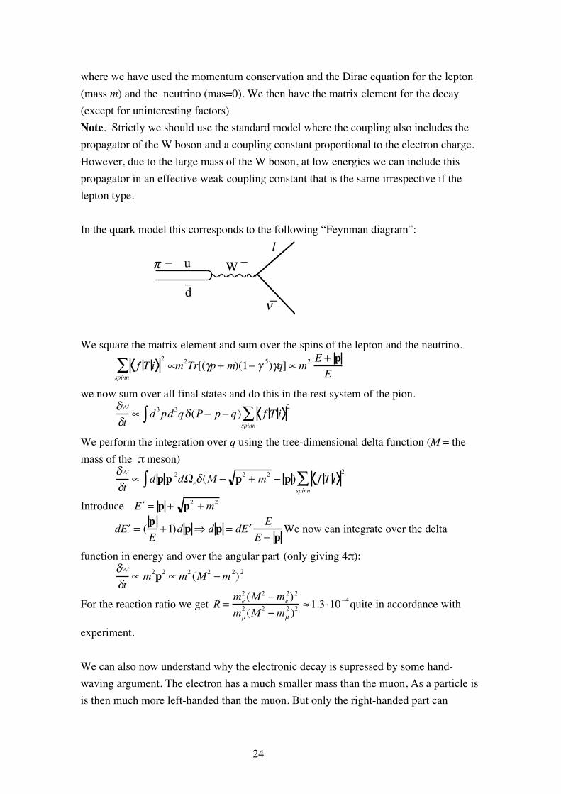
where we have used the momentum conservation and the Dirac equation for the lepton (mass m) and the neutrino (mas=0). We then have the matrix element for the decay (except for uninteresting factors) Note. Strictly we should use the standard model where the coupling also includes the propagator of the W boson and a coupling constant proportional to the electron charge. However, due to the large mass of the W boson, at low energies we can include this propagator in an effective weak coupling constant that is the same irrespective if the lepton type. In the quark model this corresponds to the following “Feynman diagram”:

We square the matrix element and sum over the spins of the lepton and the neutrino.

f T i2∝

spinn∑ m2Tr[(γp + m)(1− γ 5)γq]∝m2 E + p

E

we now sum over all final states and do this in the rest system of the pion.

δwδt

∝ d3∫ pd3qδ(P− p − q) f T i2

spinn∑

We perform the integration over q using the tree-dimensional delta function (M = the mass of the π meson)

δwδt

∝ dp∫ p 2dΩeδ(M − p2 + m2 − p ) f T i2

spinn∑

Introduce ′ E = p + p2 + m2

d ′ E = ( pE

+1)dp⇒ dp = d ′ E EE + p

We now can integrate over the delta

function in energy and over the angular part (only giving 4π):

δwδt

∝ m2p2 ∝m2 (M2 −m 2)2

For the reaction ratio we get R =me2 (M2 −me

2)2

mµ2 (M2 −mµ

2 )2≈1.3 ⋅10−4quite in accordance with

experiment. We can also now understand why the electronic decay is supressed by some hand-waving argument. The electron has a much smaller mass than the muon, As a particle is is then much more left-handed than the muon. But only the right-handed part can

π – u

d–W –

l

ν–

25

interact in the reaction. With its large mass the muon is almost at rest and is more or less equally left- and right-handed. Appendix. Local gauge invariance The Lagrangian density for a free Dirac particle is given by L = i∂µΨγ µΨ + mΨΨ Using Lagrange’s equations

∂µ

∂L∂µΨ( ) −

∂L∂Ψ

= 0

we get the Dirac equation: ∂µ iγ µΨ( )− mΨ = iγ µ ∂µ− m( )Ψ = 0 A local gauge transformation is a transformation where we do the replacement Ψ →Ψ eiqΛ(x) ,Ψ →Ψ e− iqΛ(x) It is easily seen the the Lagrangian above is not invariant under such a transformation because of the coordinate dependence on the gauge function Λ Exercise. Show this. However, if we replace the derivative according to ∂µ→ Dµ = ∂µ− iqAµ the covariant derivative, the new Lagrangian is invariant under a local gauge transformation provided that the vector field Aµ transforms according to Aµ → Aµ + ∂µΛ Proof: L = iDµΨγ µΨ + mΨΨ = i ∂µ− iqAµ( )Ψγ µΨ + mΨΨ

L → iΨ e− iΛqγ µe+ iΛq iqΨ ∂µΛ + ∂µΨ − iqAµΨ − iqΨ ∂µΛ( ) + mΨΨ We see that the offending derivative of Λ disappears and thus the new Lagrangian is invariant. The Dirac equation derived from the modified Lagrangian is then

iγ µDµ − m( )Ψ = iγ µ ∂µ− iqAµ( )− m( )Ψ = 0

The extra term in the Lagrangian is an interaction term between the electron and the vector field −qΨγ µΨ Aµ . We have earlier seen that Ψγ µΨ is the (four-dimensional) probability current so with the identification q = e we identify the quantity

Jµ = −eΨγ µΨ with the electrical current and Aµ with the electromagnetic field. We

can add a term to generate the differential equation for the electromagnetic field

14 FµνFµν , Fµν = ∂µ Aν − ∂ν Aµ

The equation for the electromagnetic field will be ∂

µ∂µ Aν =!Aν = Jν that is precisely the equation you get from Maxwell’s equations.

26

Local gauge invariance generates precisely the correct interaction between the electron and the electromagnetic field.