Embed Size (px)
Citation preview

1
Lecture 7Lecture 7From Dirac equation to From Dirac equation to Feynman diagrammsFeynman diagramms
SS2011SS2011: : ‚‚Introduction to Nuclear and Particle Physics, Part 2Introduction to Nuclear and Particle Physics, Part 2‘‘

The Dirac equation - the wave-equation for free relativistic fermions follows the requirements :
1) that the wave-equation – as in case of the Schrödinger equation – should be of1st order in ∂/∂t ≡∂/∂x0
2) to allow for a continuity equation with a positive density ψ*ψ:
3) relativistic covariance (with respect to Lorentz transformations) then requires that the wave-equation also has to be of 1st order in the spacial derivatives ∂/∂xk (k = 1, 2, 3) , i.e.:
2
Dirac equation*Dirac equation*
(1)
This equation can be rewritten in covariant notation:
* * cf. Lecture 10 WS2010/2011cf. Lecture 10 WS2010/2011

3
Dirac equationDirac equation
(2)
(3)
The covariant form of the Dirac equation:
4-momentum
4-coordinate
covariant derivative
electromagnetic 4-potential
4-current
(4)
then involves
with the four-vector coefficients
Further four-vectors are given by:

4
Dirac equationDirac equation
(7)
where we have employed the pseudometric (Lorentz invariant) tensor:
Scalar products are Lorentz invariant, e.g. the invariant mass
with
Thus we have:
(5)
(6)

5
Dirac equationDirac equation
(11)
Including the interaction with vector fields Aμ implies:
Then the Dirac equation reads:
The (anti-commutator) algebra of the γ-matrices has to follow:
with the properties:
By counting the number of boundary conditions (cf. Eq. (6) for cf. Eq. (6) for ααk, k, ββ in Lecture 10 in Lecture 10 WS2010/2011)WS2010/2011) the γ-matrices have to be 4x4 matrices and consequently the wavefunctions Ψ(x)must have 4 components
(8)
(9)
(10)

6
Dirac equationDirac equation
Then we get:
which reads explicitly:
(12)
(13)
(14)
(15)
The solution of the Dirac equation are plane waves with positive and negative energiesseparate the four components wave vector ψ into two vectors with 2 components ϕ, χ
for spin ‚up‘ and ‚down‘ (relative to the z-direction = direction of motion):
using

7
Dirac equation: fermionsDirac equation: fermions
The solution of the coupled equation (15) reads:
where σk (k=1,2,3) are the Pauli matrices.
(16)
I. Consider the positive energy
Since the components are two-vectors, we may expand them as
spin ‚up‘ spin ‚down‘N is the normalization factor
(17)

8
Dirac equation: fermionsDirac equation: fermions
Then
In matrix notation:
The solutions of the Dirac equation then read explicitlyfor fermions with spin ‚up‘ and spin ‚down‘:
(18)
(19)
(20)

8
Dirac equation: antiDirac equation: anti--fermionsfermions
II. Consider the negative energy states = anti-fermions
Using
we obtain for the anti-fermion components with spin ‚up‘ and ‚down‘:
Accordingly free (anti-)fermions are fully defined by the spinors specified above!
(21)

Commonly one uses 2 ways of normalization:
1) as in Bjorken, Drell *:
thus,
in the rest-frame (E=m):
8
Dirac equation: normalizationDirac equation: normalization
2) the normalization used here (e.g. as Aitchison, Hey):
(22)
(23)
Constrain for the normalization:
* * used in Lecture 10 WS2010/2011used in Lecture 10 WS2010/2011
(24)

8
Dirac spinorsDirac spinors
Free (anti-)fermions are fully defined by the spinors specified above (with normalization (24)):
1) Spinors with positive energy (fermions):
2) Spinors with negative energy (anti-fermions):
Wave vector ψ : fermions
anti-fermions
spin ‚up‘ : spin ‚down‘
(27)
(26)
(25)

Dirac equation: positive and negative energy statesDirac equation: positive and negative energy states
Interpretation of the solutions with positive and negative energies:
1) Dirac (1930): particle-hole picture
E > 0: particlesE < 0: hole states =anti-paticles
Dirac sea
particles
anti-particles=holes2) Feynman picture:
E<0, e<0 anti-particles: travelling back in time
Emission of an antiparticle with 4-momentum pμ is equivalent to the absorption of a particle with 4-momentum - pμ
Absorption of an antiparticle with 4-momentum pμ is equivalent to the emission of a particle with 4-momentum - pμ

13
π+ scattering
1) π+ - scatteringon a time dependent electromagnetic potential V(t)~e-iωt Interaction by
electromagnetic potential
Matrix element:
at time t : π+ -meson absorbs the photon of energy and increases its energyωh
absorbtion at time t of the photon of energy ωh

14
π - scattering
2) π - - scattering
Matrix element:
π- - scattering π + - scatteringwith positive energy with negative energy
Energy of π – is equal to the energy of π+ -meson

15
π+ π - -pair production
3) π+ π - - pair production/creation
Matrix element:
The sum of π – and π+ meson energies is equal to the energy of the absorbed photon

16
π+ π - -pair annihilation
4) π+ π - - pair annihilation
Matrix element:
The energy of π – and π+ mesons is equal to the energy of the produced photon

In order to see how to solve the inhomogenuous Dirac equation (30) for electrons in an electromagnetic field let‘s first consider the example from electrostatics -
solution of Poisson equation:
17
Dirac equation: Green functionsDirac equation: Green functionsThe Dirac equation for electrons in an electromagnetic field can be obtained from the free Dirac equation (2) by the substitution (minimal coupling)
Notation:
(28)
(29)
(30)
(31)
Here ρ(x) is the free charge density.
• For a pointlike charge, i.e.
the static Coulomb potential - solution of (31) - is known:
(32)
(33)
18
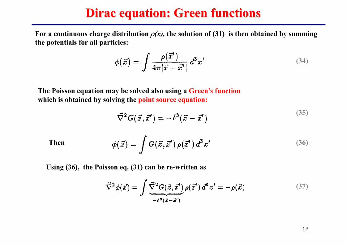
Dirac equation: Green functionsDirac equation: Green functionsFor a continuous charge distribution ρ(x), the solution of (31) is then obtained by summing the potentials for all particles:
(34)
(35)
The Poisson equation may be solved also using a Green's functionwhich is obtained by solving the point source equation:
Then (36)
Using (36), the Poisson eq. (31) can be re-written as
(37)

19
Dirac equation: Green functionsDirac equation: Green functions
(38)
The solution of eq. (36) is the spatial Green‘s function:
To solve the Dirac eq. (30) one defines the Green function K(x,x‘) (where x,x‘ are 4-vectors)by the requirement
(39)
(40)Thus, the solution of the inhomogenuous Dirac eq. (30) reads
Green function = integration kernel
Indeed:

20
Electron propagatorElectron propagator
The general solution of the inhomogenuous Dirac eq. (30) reads
homogenuous solution of free Dirac equation
inhomogenuous solution of Dirac equation with electromagnetic potential
Since the coupling constant is weak, one can use the perturbation theory:
(41)
(42)

21
Electron propagatorElectron propagator
The explicit form of the Green‘s function can be written as a Fourier transform
(42)
(43)
Substitute (42) in the eq. for the Green‘s function (39)
Multiply (43) by and one gets
(44)forElectron propagator:
Note: propagator (44) is defined only for virtual electrons, since for real electrons

22
Electron propagatorElectron propagator
Thus, the Green‘s function is
for positive energy states:
(45)
In (45) integral over p0 has 2 poles:
The integral in (45) can be evaluated by the method of residues by closing the contour in the lower(upper) half of the p0 -plane
23
Electron propagatorElectron propagator
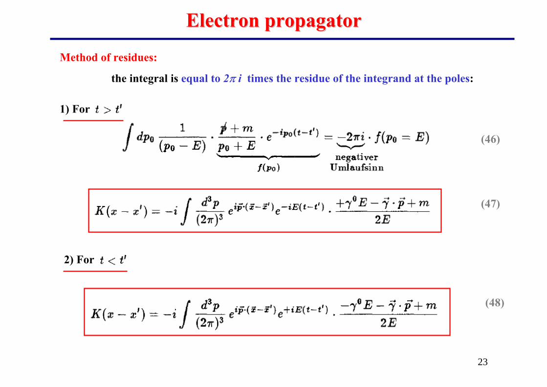
Method of residues:
the integral is equal to 2π i times the residue of the integrand at the poles:
1) For
(46)
(47)
(48)
2) For

24
Electron propagatorElectron propagator
The integral (45) can be evaluated also by integration along Re(p0) line, however, by shifting the poles by an infinitesimal positive value ε (ε 0):
(49)
Thus, the electron propagator reads:
(50)

25
Electron propagatorElectron propagator
The name ‚propagator‘ is also used for the Green‘s function since K(x,x‘) describes the propagation of the particles from x to x‘ :•The wavefunction at the final space time point x‘ w.f. of a free particle with positive energy = free plane waves:
•The wavefunction at space-time point x:
(51)
(52)
Indeed, for t > t‘ using eq.(47)
(53)

26
Electron propagatorElectron propagator
A wave function of positive energy will spread only forward in time and not backward in time, i.e. for t < t’ one gets:
Thus, for the wave function with positive energy (k0 > 0):
=0 from Dirac eq.
In a similar way one can show that for negative energy (k0 < 0) by virtue of K(x-x’) the wave function only propagates backward in time.
(54)
(55)