Embed Size (px)
Citation preview

arX
iv:h
ep-t
h/04
0727
7v4
22
Oct
200
5
The Dilatation Operatorof N = 4 Super Yang-Mills Theory
and Integrability
DissertationEingereicht an der Humboldt-Universitat zu Berlin
Uberarbeitete Fassung
O1(x) O2(y)
Niklas Beisert
22. Oktober 2005
hep-th/0407277
AEI-2004-057
Max-Planck-Institut fur GravitationsphysikAlbert-Einstein-Institut
Am Muhlenberg 1, 14476 Potsdam, Deutschland


iii
Zusammenfassung
Der Dilatationsoperator der
N = 4 Super Yang-Mills Theorie
und Integrabilitat
Der Dilatationsoperator mißt Skalendimensionen von lokalen Operatoren in einer konfor-men Feldtheorie. In dieser Dissertation betrachten wir ihn am Beispiel der maximal super-symmetrischen Eichtheorie in vier Raumzeit-Dimensionen. Wir entwicken und erweiternTechniken um den Dilatationsoperator abzuleiten, zu untersuchen und anzuwenden. DieseWerkzeuge sind ideal geeignet um Prazisionstests der dynamischen AdS/CFT-Vermutunganzustellen. Insbesondere wurden er im Zusammenhang mit Stringtheorie auf dem plane-waves Hintergrund (ebenfrontige planare Wellen) und dem Thema spinning strings erfol-greich angewendet.
Wir konstruieren den Dilatationsoperator ausschließlich mittels algebraischer Metho-den: Indem wir die Symmetriealgebra und strukturelle Eigenschaften von Feynman-Dia-grammen ausnutzen, konnen wir aufwendige, feldtheoretische Berechnungen auf hoherenSchleifen umgehen. Auf diese Weise erhalten wir den kompletten ein-schleifen Dilata-tionsoperator und die planare drei-schleifen Deformation in einem interessanten Untersek-tor. Diese Resultate erlauben es uns auf das Thema Integrabilitat in vier-dimensionalenplanaren Eichtheorien einzugehen: Wir beweisen, daß der komplette Dilatationsopera-tor auf einer Schleife integrabel ist, und prasentieren den dazugehorigen Bethe-Ansatz.Weiterhin argumentieren wir, daß die Integrabilitat sich bis drei Schleifen und daruberhinaus fortsetzt. Unter der Annahme der Integrabilitat konstruieren wir schließlich einneuartiges Spinketten-Modell auf funf Schleifen und schlagen einen Bethe-Ansatz vor, dersogar auf beliebig vielen Schleifen gultig sein mag!
Wir veranschaulichen den Nutzen unserer Methoden in zahlreichen Beispielen undstellen zwei wichtige Anwendungen im Rahmen der AdS/CFT-Korrespondenz vor: Wirleiten aus dem Dilatationsoperator den Hamiltonoperator der plane-wave String-Feld-theorie her und berechnen damit die Energieverschiebung auf dem Torus. Weiterhinwenden wir den Bethe-Ansatz an, um Skalendimensionen von Operatoren mit großenQuantenzahlen zu finden. Der Vergleich mit der Energie von spinning strings Konfigura-tionen zeigt eine erstaunliche Ubereinstimmung.

iv
Abstract
The dilatation generator measures the scaling dimensions of local operators in a con-formal field theory. In this thesis we consider the example of maximally supersymmetricgauge theory in four dimensions and develop and extend techniques to derive, investigateand apply the dilatation operator. These tools are perfectly suited for precision tests ofthe dynamical AdS/CFT conjecture. In particular, they have been successfully appliedin the context of strings on plane waves and spinning strings.
We construct the dilatation operator by purely algebraic means: Relying on the sym-metry algebra and structural properties of Feynman diagrams we are able to bypassinvolved, higher-loop field theory computations. In this way we obtain the completeone-loop dilatation operator and the planar, three-loop deformation in an interestingsubsector. These results allow us to address the issue of integrability within a planarfour-dimensional gauge theory: We prove that the complete dilatation generator is inte-grable at one-loop and present the corresponding Bethe ansatz. We furthermore arguethat integrability extends to three-loops and beyond. Assuming that it holds indeed, wefinally construct a novel spin chain model at five-loops and propose a Bethe ansatz whichmight be valid at arbitrary loop-order!
We illustrate the use of our technology in several examples and also present two keyapplications for the AdS/CFT correspondence: We derive the plane-waves string fieldtheory Hamiltonian from the dilatation operator and compute the energy shift on thetorus. Furthermore, we use the Bethe ansatz to find scaling dimensions of operators withlarge quantum numbers. A comparison to the energy of spinning strings shows an intricatefunctional agreement.

v
Contents
Title i
Zusammenfassung iii
Abstract iii
Contents v
Introduction 1
Overview 13
1 Field Theory and Symmetry 15
1.1 N = 4 Super Yang-Mills Theory . . . . . . . . . . . . . . . . . . . . . . . . 151.2 The Quantum Theory . . . . . . . . . . . . . . . . . . . . . . . . . . . . . 191.3 The Gauge Group . . . . . . . . . . . . . . . . . . . . . . . . . . . . . . . . 221.4 The ’t Hooft Limit . . . . . . . . . . . . . . . . . . . . . . . . . . . . . . . 241.5 The Superconformal Algebra . . . . . . . . . . . . . . . . . . . . . . . . . . 251.6 Fields and States . . . . . . . . . . . . . . . . . . . . . . . . . . . . . . . . 281.7 Highest-Weight Modules and Representations . . . . . . . . . . . . . . . . 291.8 Unitarity and Multiplet Shortenings . . . . . . . . . . . . . . . . . . . . . . 311.9 The Field-Strength Multiplet . . . . . . . . . . . . . . . . . . . . . . . . . 331.10 Correlation Functions . . . . . . . . . . . . . . . . . . . . . . . . . . . . . . 341.11 The Current Multiplet . . . . . . . . . . . . . . . . . . . . . . . . . . . . . 36
2 The Dilatation Operator 39
2.1 Scaling Dimensions . . . . . . . . . . . . . . . . . . . . . . . . . . . . . . . 392.2 Perturbation Theory . . . . . . . . . . . . . . . . . . . . . . . . . . . . . . 452.3 Subsectors . . . . . . . . . . . . . . . . . . . . . . . . . . . . . . . . . . . . 502.4 The su(2) Quarter-BPS Sector . . . . . . . . . . . . . . . . . . . . . . . . . 552.5 Field Theoretic Considerations . . . . . . . . . . . . . . . . . . . . . . . . . 612.6 The Planar Limit and Spin Chains . . . . . . . . . . . . . . . . . . . . . . 65

vi Contents
3 One-Loop 71
3.1 The Form of the Dilatation Generator . . . . . . . . . . . . . . . . . . . . 713.2 The Fermionic su(1, 1)× u(1|1) Subsector . . . . . . . . . . . . . . . . . . 743.3 The Lift to psu(2, 2|4) . . . . . . . . . . . . . . . . . . . . . . . . . . . . . 793.4 The Bosonic su(1, 1) Subsector . . . . . . . . . . . . . . . . . . . . . . . . . 803.5 Planar Spectrum . . . . . . . . . . . . . . . . . . . . . . . . . . . . . . . . 813.6 Plane Wave Physics . . . . . . . . . . . . . . . . . . . . . . . . . . . . . . . 88
4 Integrability 95
4.1 Integrable Spin Chains . . . . . . . . . . . . . . . . . . . . . . . . . . . . . 954.2 One-Loop Integrability . . . . . . . . . . . . . . . . . . . . . . . . . . . . . 1014.3 The Algebraic Bethe Ansatz . . . . . . . . . . . . . . . . . . . . . . . . . . 1054.4 Spectrum . . . . . . . . . . . . . . . . . . . . . . . . . . . . . . . . . . . . 1134.5 The Thermodynamic Limit . . . . . . . . . . . . . . . . . . . . . . . . . . . 1154.6 Stringing Spins . . . . . . . . . . . . . . . . . . . . . . . . . . . . . . . . . 118
5 Higher-Loops 125
5.1 The su(2|3) Eighth-BPS Sector . . . . . . . . . . . . . . . . . . . . . . . . 1255.2 Tree-Level . . . . . . . . . . . . . . . . . . . . . . . . . . . . . . . . . . . . 1295.3 One-Loop . . . . . . . . . . . . . . . . . . . . . . . . . . . . . . . . . . . . 1305.4 Two-Loops . . . . . . . . . . . . . . . . . . . . . . . . . . . . . . . . . . . . 1345.5 Three-Loops . . . . . . . . . . . . . . . . . . . . . . . . . . . . . . . . . . . 1385.6 Spectrum . . . . . . . . . . . . . . . . . . . . . . . . . . . . . . . . . . . . 139
6 Higher-Loop Integrability 149
6.1 Higher-Loop Spin Chains . . . . . . . . . . . . . . . . . . . . . . . . . . . . 1496.2 The su(2) Sector at Higher-Loops . . . . . . . . . . . . . . . . . . . . . . . 1546.3 Spectrum . . . . . . . . . . . . . . . . . . . . . . . . . . . . . . . . . . . . 1616.4 Long-Range Bethe Ansatz . . . . . . . . . . . . . . . . . . . . . . . . . . . 1656.5 Stringing Spins at Higher Loops . . . . . . . . . . . . . . . . . . . . . . . . 171
Conclusions 177
Outlook 181
A An Example 185
A.1 Non-Planar Application . . . . . . . . . . . . . . . . . . . . . . . . . . . . 185A.2 Planar Application . . . . . . . . . . . . . . . . . . . . . . . . . . . . . . . 186
B Spinors in Various Dimensions 189
B.1 Four Dimensions . . . . . . . . . . . . . . . . . . . . . . . . . . . . . . . . 189B.2 Six Dimensions . . . . . . . . . . . . . . . . . . . . . . . . . . . . . . . . . 189B.3 Ten Dimensions . . . . . . . . . . . . . . . . . . . . . . . . . . . . . . . . . 190
C SYM in Ten Dimensions 191
C.1 Ten-Dimensional Gauge Theory in Superspace . . . . . . . . . . . . . . . . 191C.2 Ten-Dimensional Gauge Theory in Components . . . . . . . . . . . . . . . 192C.3 N = 4 SYM from Ten Dimensions . . . . . . . . . . . . . . . . . . . . . . . 193

Contents vii
D The Algebra u(2, 2|4) 195
D.1 Commutation Relations . . . . . . . . . . . . . . . . . . . . . . . . . . . . 195D.2 Labels . . . . . . . . . . . . . . . . . . . . . . . . . . . . . . . . . . . . . . 196D.3 The Quadratic Casimir . . . . . . . . . . . . . . . . . . . . . . . . . . . . . 197D.4 The Oscillator Representation . . . . . . . . . . . . . . . . . . . . . . . . . 197
E Tools for the su(2) Sector 201
E.1 States . . . . . . . . . . . . . . . . . . . . . . . . . . . . . . . . . . . . . . 201E.2 Interactions . . . . . . . . . . . . . . . . . . . . . . . . . . . . . . . . . . . 201E.3 Spectrum . . . . . . . . . . . . . . . . . . . . . . . . . . . . . . . . . . . . 202E.4 An Example . . . . . . . . . . . . . . . . . . . . . . . . . . . . . . . . . . . 202E.5 Commutators . . . . . . . . . . . . . . . . . . . . . . . . . . . . . . . . . . 203
F The Harmonic Action 205
F.1 Generic Invariant Action . . . . . . . . . . . . . . . . . . . . . . . . . . . . 205F.2 The Harmonic Action . . . . . . . . . . . . . . . . . . . . . . . . . . . . . . 205F.3 Proof . . . . . . . . . . . . . . . . . . . . . . . . . . . . . . . . . . . . . . . 206F.4 An Example . . . . . . . . . . . . . . . . . . . . . . . . . . . . . . . . . . . 207
Acknowledgements a
References c

viii

1
Introduction
Probably the two most important advances in the deeper understanding of our worldin terms of theoretical physics were made at the beginning of the twentieth century: Thetheory of general relativity and quantum mechanics. On the one hand, Einstein’s theory ofgeneral relativity (GR) has replaced Newton’s theory of gravity and, in its original form, isstill the most accurate theory to describe forces between massive bodies. It brought abouta major change in the notion of space and time. Both were unified into spacetime which,in addition, is curved by the masses that propagate on it. Two of the most importantconceptual improvements of GR are symmetry and locality. The symmetry of GR is calleddiffeomorphism-invariance and allows to label points of spacetime in an arbitrary way, theequations of GR do not depend on this. Furthermore, GR is a local field theory, thereis no action at a distance, but instead, just like in Maxwell’s Electrodynamics, forces aremediated by a field.
On the other hand, there is Quantum Mechanics. It proposes a completely new notionof particles and forces, both of which should be considered as two manifestations of thesame object. It also departed from a deterministic weltanschauung; a measurement isinevitably probabilistic and moreover must be considered as an action which influencesthe outcome of future measurements. Many aspects of quantum mechanics seem odd atfirst and second sight and truly make sense only in a quantum field theory (QFT). QFTintroduced the notion of particle creation and annihilation, an essential element for localinteractions. The price that has to be paid are spurious divergencies due to particlesbeing created and annihilated at the same place and instant. It required some effort tounderstand, regularise and renormalise the divergencies in order to obtain finite, physicalresults.
The first fully consistent physical QFT was Quantum Electrodynamics (QED), thequantum counterpart of Electrodynamics. A guiding principle in the construction ofQED is, again, symmetry. Here, the symmetry is given by gauge transformations; theyallow to change some unphysical degrees of freedom of the theory by an arbitrary amount.Consequently, QED is termed a gauge theory and, in particular, it has an Abelian U(1)gauge group. Amplitudes in QED can be expanded in a coupling constant g related to thefundamental charge of an electron. This perturbative treatment leads to Feynman dia-grams which describe interactions in a rather intuitive fashion. Besides electromagnetism,two other interactions between particles have been observed in particle accelerators: theweak and the strong interactions. Let us discuss the second kind. The strong nuclearforce is responsible for the binding of nucleons to nuclei, which would otherwise dispersedue to their electromagnetic charge. One of the earlier candidates for a description ofthese interactions was a string theory, a theory of string-like extended objects instead ofpoint-like particles. It explained some qualitative aspects of particle (excitation) spectra

2 Introduction
correctly; yet, soon it was found that it embodies some insurmountable theoretical as wellas phenomenological shortcomings and interest in it declined.
In the meantime, an alternative description of strong (and weak) interactions hademerged. Like QED, it is based on a gauge theory, the so-called Quantum Chromody-namics (QCD). The gauge group for strong interactions is SU(3), which may, for instance,be inferred indirectly from the spectrum of hadrons. Here, symmetry is important for sev-eral reasons. First of all, and even more so for QCD than for QED, symmetry is essentialfor the theoretical consistency of the model. Furthermore, the particular gauge group ofQCD leads to a feature called asymptotic freedom/confinement. It implies that QCD iseffectively weak at very short distances, but becomes infinitely strong at larger dimensions(on the scale of nucleons). On a qualitative level, this may be understood as follows: Theattraction/repulsion between two charges is mediated by flux lines. As opposed to QED,in QCD flux lines attract each other and will form a small tube stretching between thecharges. The tube effectively behaves like a string with tension and binds the particlesirrespective of their distance. This explains why it is not possible to observe an individualcharged particle and leads us to confinement, which allows only uncharged particles topropagate freely.
A peculiarity of generic gauge theories with gauge group U(N), which we will makeheavy use of, was observed by ’t Hooft [1]: He derived a relationship between the topolog-ical structure of a Feynman graph and its N -dependence. When 1/N is interpreted as acoupling constant, he observed that the perturbative expansion in 1/N is very similar innature to the perturbative genus expansion in a generic interacting string theory (stringfield theory).
Not only due to their mathematical beauty, the theory of General Relativity andQuantum Mechanics/QFT have become the foundations of modern physics, but mainlybecause of the accuracy to which they describe the world. On the one hand, gravity is avery weak force and it requires a large amount of matter to feel its effects. Consequently,GR describes the world at very large scales. For instance, GR was first confirmed when theaberration of light near the perimeter of the sun was investigated. On the other hand, theremaining three forces described by QFT’s are incomparably stronger. Therefore quantumfield theories chiefly describe the microcosm. In particular, the standard model of particlephysics, the union of the above three gauge theories, has led to some non-trivial predictionswhich have been confirmed with unprecedented accuracy, e.g. the electric moment of theelectron and muon.
One of the major open problems of theoretical physics is to understand what happenswhen an enormous amount of matter is concentrated on a very small region of space. Forexample, this situation arises at the singularity of a black hole or shortly after the bigbang. To describe such a situation, we would need to combine General Relativity withthe concepts of quantum field theory and consider quantum gravity (QG). Despite thebetter part of a century of research, such a unification correctly describing our world hasnot yet been found. The main obstacle for the direct construction of a quantum theory ofgravity are the divergencies mentioned above, which cannot be renormalised in this caseand render the quantum theory meaningless.
Currently, the most favoured theory for a consistent quantisation of gravity is su-perstring theory. It is a refinement of the (bosonic) string theory found in connectionwith strong interactions and involves an additional symmetry which relates fermions and

Introduction 3
bosons, namely supersymmetry. Supersymmetry makes string theory very appealing totheorists: It overcomes several of the shortcomings of bosonic string theory and restrictsthe form such that there are only five types of string theories (IIA,IIB,I,HO,HE), whichwere, moreover, argued to be equivalent via duality. This is a very good starting point fora theory of everything, given that string theory not only naturally incorporates gravity,but also gauge theories, the type of theory on which the standard model is based.
With the advent of superstring theory, supersymmetry has been applied to field the-ories as well, giving rise to beautiful structures. One important aspect is that many ofthe divergencies observed in ordinary QFT’s are absent in supersymmetric ones. Indeed,this is the case for the unique, maximally supersymmetric gauge theory in four spacetimedimensions, N = 4 super Yang-Mills theory (N = 4 SYM) [2]. This remarkable feature [3]allows the theory to be conformally invariant, even at the quantum level! Conformal sym-metry is a very constraining property in field theory. Most importantly, two-point andthree-point correlation functions are completely determined by the scaling dimensions andstructure constants of the involved local operators. For instance, the two-point functionof a scalar operator O of dimension D must be of the form
⟨O(x)O(y)
⟩=
M
|x− y|2D , (1)
whereM is an unphysical normalisation constant. In two dimensions, conformal symmetryis even more powerful, it makes a theory mathematically quite tractable and leads to anumber of exciting phenomena such as integrability. Consequently, it plays a major rolein the world-sheet description of string theory and was thoroughly investigated. In fourdimensions, however, conformal invariance appeared to be more of a shortcoming at firstsight: It makes the model incompatible with particle phenomenology, which might be thereason why N = 4 SYM was abandoned soon after its discovery.
New interest in this theory was triggered by the AdS/CFT correspondence. Inspired bythe studies of string/string dualities and D-branes, Maldacena conjectured that IIB stringtheory on the curved background1 AdS5 × S5 should be equivalent to N = 4 SYM [4–6](see [7] for comprehensive reviews of the subject) and thus substantiated the gauge/stringduality proposed earlier by ’t Hooft. The correspondence is supported by the well-knownfact that the symmetry groups of both theories, PSU(2, 2|4), match. Consequently, therepresentation theory of the superconformal algebra psu(2, 2|4) [8] was investigated moreclosely [9, 10], and numerous non-renormalisation theorems were derived (see e.g. [11]).In addition, some unexpected non-renormalisation theorems, which do not follow frompsu(2, 2|4) representation theory, were found [12]. Once thought to be somewhat boring,it gradually became clear that conformal N = 4 gauge theory is an extremely rich andnon-trivial theory with many hidden secrets; eventually, the correspondence has helpedin formulating the right questions to discover some of them.
Yet, the conjecture goes beyond kinematics and claims the full dynamical agreementof both theories. For example, it predicts that the spectrum of scaling dimensions D inthe conformal gauge theory should coincide with the spectrum of energies E of stringstates
{D} = {E}. (2)
1This manifold consists of the five-sphere and the five-dimensional anti-de Sitter spacetime, which isan equivalent of hyperbolic space but with Minkowski signature.

4 Introduction
Unfortunately, like many dualities, Maldacena’s conjecture is of the strong/weak type:The weak coupling regime of gauge theory maps to the strong coupling (i.e. tensionless)regime in string theory and vice versa. The precise correspondence is given by
g2YMN = λ =
R4
α′ 2 ,1
N=
4πgs
λ, (3)
where gYM is the Yang-Mills coupling constant and α′ is the inverse string tension.2 Fur-thermore, N is the rank of the U(N) gauge group of Yang-Mills theory, λ is the effective’t Hooft coupling constant in the large N limit, gs is the topological expansion parame-ter in string theory and R is the radius of the AdS5 × S5 background. It is not knownhow to fully access the strong coupling regime in either theory, let alone how to rigor-ously quantise string theory on the curved background. Therefore, the first tests of theAdS/CFT correspondence were restricted to the infinite tension regime of string theorywhich is approximated by supergravity and corresponds to the strong coupling regime onthe gauge theory side. Gauge theory instanton calculations of four-point functions of op-erators which are protected by supersymmetry were shown to agree with the supergravityresults see e.g. [13].
Despite a growing number of confirmations of the conjecture in sectors protected bysymmetry, the fundamental problem of a strong/weak duality remained. For example, theAdS/CFT correspondence predicts that the scaling dimensions D of generic, unprotectedoperators in gauge theory should scale as
D ∼ λ1/4 (4)
for large λ, but how could this conjecture be tested? It was Berenstein, Maldacena andNastase (BMN) who proposed a limit where this generic formula may be evaded [14]: Inaddition to a large λ, consider local operators with a large charge J on S5, whose scalingdimension D is separated from the charge J by a finite amount only. More explicitly, thelimit proposed by BMN is
λ, J −→∞ with λ′ =λ
J2and D − J finite. (5)
In this limit, the AdS5 × S5 background effectively reduces to a so-called plane-wavebackground [15] on which the spectrum of string modes can be found exactly and thetheory can be quantised [16]. Remarkably, the light-cone energy ELC of a string-modeexcitation
ELC =√
1 + λ′n2 = 1 + 12λ′n2 + . . . (6)
has a perturbative expansion at a small effective coupling constant λ′. As the light-coneenergy corresponds to the combination D−J in gauge theory, suddenly the possibility ofa quantitative comparison for unprotected states had emerged! Indeed, BMN were able toshow the agreement at first order in λ′ for a set of operators. Their seminal article [14] hassparked a long list of further investigations and we would like to refer the reader to [17]for reviews. Let us only comment on one direction of research: In its original form, theBMN limit was proposed only for non-interacting strings and gauge theory in the planar
2The actions are inversely related to these constants, SYM ∼ 1/g2YM
and Sstring ∼ 1/α′. Therefore,quantum effects are suppressed at small gYM and small α′ in the respective theories.
Introduction 5
limit. Soon after the BMN proposal, it was demonstrated that also non-planar correctionscan be taken into account in gauge theory [18, 19], they correspond to energy shifts dueto string interactions [20]. In gauge theory, the effective genus counting parameter inthe so-called double-scaling limit is g2 = J2/N . The first order correction in λ′ and g2
2
was computed in [21, 22] and was argued to agree with string theory [23, 24]. This is yetanother confirmation of the AdS/CFT correspondence, but for the first time within aninteracting string theory!
In the study of the BMN correspondence, the attention has been shifted away fromlower dimensional operators to operators with a large number of constituent fields [18,19,21,22,25]. There, the complications are mostly of a combinatorial nature. It was thereforedesirable to develop efficient methods to determine anomalous dimensions without havingto deal with artefacts of the regularisation procedure. This was done in various papers,on the planar [14,25–28] and non-planar level [18,19,21,22,29,30], extending earlier workon protected half-BPS [31–33] and quarter-BPS operators [34]. In [35] it was realised,following important insights in [36,37], that these well-established techniques can be con-siderably simplified and extended by considering the Dilatation Operator. The dilatationoperator D is one of the generators of the conformal algebra and it measures the scalingdimension D of a local operator3 O
DO = DO. (7)
In general, there are many states and finding the scaling dimension is an eigenvalueproblem which requires to resolve the mixing of states. Once the dilatation operator hasbeen constructed, it will generate the matrix of scaling dimensions for any set of localoperators of a conformal field theory in a purely algebraic way (in App. A we present anintroductory example of how to apply the dilatation operator). What is more, scalingdimensions can be obtained exactly for all gauge groups and, in particular, for the groupU(N) with finite N [38]. Even two or higher-loop calculations of anomalous dimensions,which are generically plagued by multiple divergencies, are turned into a combinatorialexercise! Using the dilatation operator techniques, many of the earlier case-by-case studiesof anomalous dimensions [33,39–46] were easily confirmed [38]. They furthermore enableda remarkable all-genus comparison between BMN gauge theory and plane-wave stringtheory [47]. The subject of this dissertation is the construction and investigation of thedilatation operator in N = 4 SYM, a conformal quantum field theory, in perturbationtheory.
Classical scaling dimensions of states are easily found by counting the constituent fieldsweighted by their respective scaling dimensions. It is just as straightforward to constructthe classical dilatation operator to perform this counting. Scaling dimensions in a fieldtheory generally receive quantum corrections, D = D(g) and consequently the dilatationoperator must receive radiative corrections D = D(g), too. In the path integral frameworkthere will be no natural way to obtain quantum corrections to the dilatation operator;we will have to derive them from correlators, for example from two-point functions. Nowwhat is the benefit in considering the dilatation operator if a conventional calculationuses two-point correlators as well? There are two major advantages: Firstly, the dilatationgenerator is computed once and for all, while a two-point function will have to be evaluated
3To avoid confusion, we will later speak of ‘states’ instead of local operators.

6 Introduction
for each pair of states (unless one makes use of some effective vertex e.g. [21,22]). Secondly,the dilatation operator computes only the scaling dimension D(g). The two-point functionalso includes a contribution M(g) from the normalisation of states. These two quantitieswill have to be disentangled before the scaling dimension can be read off from the two-pointfunction (1). Here, a complicating issue is that in general the normalisation coefficientM(g) obtained in field theory is divergent.
A radiative correction to the dilatation operator in the context of N = 4 SYM hasfirst been computed in [48, 35].4 This one-loop correction was restricted to the sector ofstates composed from the six scalar fields of the theory only, the so-called so(6) subsector,on which the one-loop dilatation operator closes.
However, there is nothing special about the scalar fields, except maybe their conceptualsimplicity. Generic local operators can as well consist of fermions or gauge fields (inthe guise of a field strength). What is more, we can also apply an arbitrary numberof (covariant) derivatives to the basic constituent fields. In principle, one could nowcompute the one-loop dilatation operator for all fields (we shall denote a generic fieldwith derivatives by the symbol W). This is feasible, but certainly much more involvedthan the calculations for the so(6) subsector due to infinitely many types of fieldsW and acomplicated structure of spacetime indices in the expected conformal two-point function,see e.g. [30, 28, 49].
In [38] a different approach to obtain contributions to the dilatation generator hasbeen proposed: Just as in field theory, all contributing diagrams to a two-point functionare written down. The most complicated part of their computation is to evaluate thespacetime integrals due to vertices of the Feynman diagram. Nevertheless, the structuralresult of the integrals is known; it is some power of the distance |x− y|a of the local oper-ators multiplied to some function f(ǫ) of the regulator.5 The power a can be inferred bymatching dimensions, but the function f(ǫ) is a genuine result of the integral. The crucialidea is not to compute the function, but to assume the most general singular behaviourwhen the regulator is removed, e.g. f(ǫ) = c−1/ǫ + c0 + c1ǫ + . . . . This allows to writedown the contributions to the dilatation operator in terms of the unknown coefficients ck.Now one can investigate the structure of the dilatation generator to simplify and combinethe contributions. Usually, it turns out that there are only a few independent coefficientswhich actually contribute to anomalous dimensions. The proposed trick is to make use ofknown results or other constraints to determine these coefficients.
To derive the complete one-loop dilatation operator, it is useful to consider its sym-metry. A common practice in physics is to derive some result only for one component of amultiplet of objects; symmetry will then ensure that the result applies to all componentsof the same multiplet. The same simplification can be applied to the one-loop dilatationoperator: It was shown in [50] that superconformal symmetry considerably reduces thenumber of independent coefficients to just a single infinite sequence. This sequence wassubsequently evaluated in field theory. Furthermore, it was conjectured that this laststep might be unnecessary and making full use the symmetry algebra would constrainthe complete one-loop dilatation operator uniquely up to an overall constant (the couplingconstant). This is indeed the case as we shall prove in this work. Put differently, su-
4Note that the correction is precisely given by the effective vertices found earlier in [19, 21].5For integrals with open spacetime indices the result is a linear combination of such terms with
spacetime indices on (x− y)µ or ηµν .

Introduction 7
perconformal symmetry and some basic facts from field theory (i.e. the generic structureof a one-loop contribution) completely determine all two-point functions at the one-looplevel! To outline the form of the dilatation operator, let us just note that the radiativecorrection acts on two fields at a time. The contribution D12 from a pair of fields dependson their ‘total spin’6 j; it is proportional to the harmonic number
D12 ∼ h(j) =
j∑
k=1
1
k. (8)
Inspired by the strongly constraining nature of the superconformal algebra at one-loop,it is natural to expect it to be very powerful at higher-loops as well. This is a very excitingprospect, since direct higher-loop computations are exceedingly labourious and not muchis known beyond the one-loop level. Although one might think that one-loop accuracyis sufficient for many purposes, one should keep in mind that it is only the first non-trivial order. Easily one can imagine some unexpected behaviour at next-to-leading orderand, indeed, we shall encounter an example of a mismatch starting only at three-loops.Furthermore, taken that the one-loop dilatation operator is completely constrained, thereis hardly any freedom for the quantum theory to decide in either direction. Therefore,a one-loop computation does not provide much information about the quantum theoryitself.
The trick of writing down the most general structure for the dilatation operator with anumber of undetermined coefficients can be used at higher-loops as well. We will, however,not try to generalise the complete dilatation operator to higher-loops. The derivation ofthe one-loop computation depends heavily on a particular feature of perturbation theorywhich allows us to restrict to classical superconformal invariance. Unfortunately, it doesnot apply at higher-loops and we would be left with a very large number of independentcoefficients to be fixed. To obtain some higher-loop results with as little work as possible,we may restrict to a subsector. The so(6) subsector of scalar fields, however, is notsuitable, there will be mixing with states involving fermions and other fields; only atone-loop it happens to be closed. To proceed to higher-loops, one could therefore restrictto an even smaller subsector. This so-called su(2) subsector consists of only two chargedscalar fields (which we shall denote by Z and φ) and charge conservation protects thestates from mixing with more general states. Here we can derive the two-loop dilatationoperator by employing some known results without performing a full-fledged two-loopfield theory computation [38].
We cannot go much further at the moment because there are no known results besidesa few basic facts from representation theory. Symmetry is not very constraining in thesu(2) sector because the dilatation operator is abelian and not part of a bigger algebra.A better choice is the su(2|3) subsector: It consists of only five fields and the symmetryalgebra includes the dilatation generator. These properties make it both, convenient tohandle and sufficiently constraining. Furthermore, not only the dilatation generator, butalso the other generators of the algebra receive radiative corrections, a generic feature ofthe higher-loop algebra. In [51] this subsector was investigated in the planar limit and
6The total spin is a quantity of the representation theory of the superconformal symmetry similar tothe total spin of the rotation group.
8 Introduction
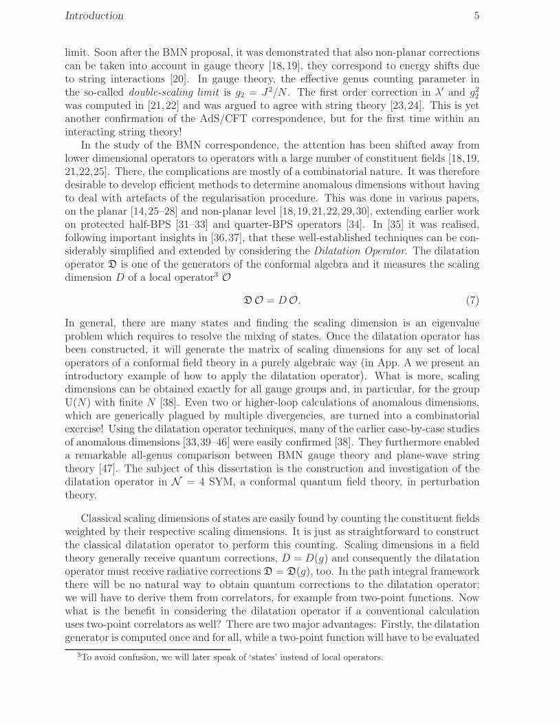
up to three-loops with an astonishing result: Although there are hundreds of independentcoefficients at three-loops, closure of the symmetry algebra
[JM(g), JN(g)
}= FPMN JP (g) (9)
constrains nearly all of them in such a way that only a handful remain. Moreover, allof them can be related to symmetries of the defining equations. Again, symmetry incombination with basic field theory provides a unique answer.
Spectral studies of all the above radiative corrections to the dilatation operator reveala property with tremendous importance: One finds a huge amount of pairs of states O±whose scaling dimensions are exactly degenerate in the planar limit
D+ = D−. (10)
This would not be remarkable if there was an obvious symmetry to relate those states.This symmetry, however, cannot be superconformal symmetry (or any subalgebra) fortwo reasons. Firstly, the degeneracy is actually broken by non-planar corrections whilesuperconformal symmetry is exact. Secondly, the degenerate states have a different paritywhich is preserved by superconformal transformations. Here, as in the remainder ofthis thesis, parity refers to complex conjugation of the SU(N) gauge group. To explainthe degeneracy we need some generator Q which inverts parity and commutes with thedilatation generator.
This curiosity of the spectrum is merely the tip of an iceberg; it will turn out that theconjectured generatorQ is part of an infinite set of commuting charges due to integrability.Integrability of a planar gauge theory will be the other major topic of this dissertation.The statement of integrability is equivalent to the existence of an unlimited number ofcommuting scalar charges Qr
[Qr,Qs] = [J,Qr] = 0. (11)
The planar dilatation operator δD = g2Q2 is related to the second charge Q2. It turnsout that the odd charges are parity odd, therefore the existence of the charge Q = Q3
explains the pairing of states. Only a few states have no partner and are unpaired.Integrable structures play a crucial role in two dimensional field theories. One of the
many intriguing features of two-dimensional CFT’s is that they are intimately connectedto integrable 2+0 dimensional lattice models in statistical mechanics or, equivalently, to1+1 dimensional quantum spin chains. The infinite set of charges is directly related tothe infinite-dimensional conformal (Virasoro) algebra in D = 2. Given the huge success inunderstanding CFT’s in two dimensions, one might hope that at least some of the aspectsallowing their treatment might fruitfully reappear in four dimensions. One might wonderabout standard no-go theorems that seem to suggest that integrability can never existabove D = 2. These may be potentially bypassed by the fact that there appears to be ahidden ‘two-dimensionality’ in U(N) gauge theory when we look at it at large N whereFeynman diagrams can be classified in terms of two-dimensional surfaces.
The first signs of integrability in N = 4 gauge theory were discovered by Minahanand Zarembo [48]. They found that the planar one-loop dilatation operator in the so(6)sector is isomorphic to the Hamiltonian of a so(6) integrable quantum spin chain. The

Introduction 9
analogy between planar gauge theory and spin chains is as follows: In the strict large Nlimit, the structure of traces within local operators cannot be changed and therefore wemay consider each trace individually or, for simplicity, only single-trace states. We theninterpret the trace as a cyclic spin chain and the fields within the trace are the spinsites. For example, the su(2) sector with two fields Z, φ maps directly to the Heisenbergspin chain, in which the spin at each site can either point up (Z) or down (φ). Forthe so(6) sector one considers a more general spin chain for which the spin can pointin six distinct abstract directions. The spin chain Hamiltonian alias the planar one-loopdilatation generator acts on the spin chain and returns a linear combination of states. Theaction is of a nearest-neighbour type, it can only modify two adjacent spins at a time.Likewise the higher charges Qr act on r adjacent spins and are therefore local (along thespin chain).
Integrable spin chains had appeared before in four-dimensional gauge theories throughthe pioneering work of Lipatov on high energy scattering in planar QCD [52]. The modelwas subsequently identified as a Heisenberg sl(2) spin chain of non-compact spin zero[53]. More recently, and physically closely related to the present study, further integrablestructures were discovered in the computation of planar one-loop anomalous dimensionsof various types of operators in QCD [54] (see also the review [55]).7
The full symmetry algebra of SYM is neither so(6) nor sl(2), but the full supercon-formal algebra psu(2, 2|4). If the discovered integrable structures are not accidental, weshould expect that the so(6) results of [48] and the sl(2) results suggested from one-loopQCD [54,55] (see also [43,57]) can be combined and ‘lifted’ to a full psu(2, 2|4) super spinchain. Indirect evidence can be obtained by the investigation of the spectrum of anoma-lous dimensions. As we have mentioned above, the occurrence of pairs of states hintsat the existence of at least one conserved charge. Indeed, the spectrum of the completeone-loop planar dilatation operator displays many such pairs. Obviously, they are foundin the so(6) and sl(2) subsectors where integrability is manifest, but also generic states dopair up. Subsequently, it was shown in [58] that the complete one-loop planar dilatationoperator is isomorphic to a psu(2, 2|4) supersymmetric spin chain.
Integrability is not merely an academic issue, for it opens the gates for very precise testsof the AdS/CFT correspondence. It is no longer necessary to compute and diagonalisethe matrix of anomalous dimensions. Instead, one may use the Bethe ansatz (c.f. [59] for apedagogical introduction) to obtain the one-loop anomalous dimensions directly [48, 58].In the thermodynamic limit of very long spin chains, which is practically inaccessibleby conventional methods, the algebraic Bethe equations turn into integral equations.With the Bethe ansatz at hand, it became possible to compute anomalous dimensions ofoperators with large spin quantum numbers [60].
Via the AdS/CFT correspondence, these states correspond to highly spinning stringconfigurations. Even though quantisation of string theory on AdS5 × S5 is an openproblem, these spinning strings can be treated in a classical fashion, c.f. [61, 62], wheninterested in the leading large spin behaviour. It was shown by Frolov and Tseytlin [63,64]that quantum (1/
√λ) corrections in the string theory sigma model are suppressed by
powers of 1/J , where J is a large spin on the five-sphere S5. In direct analogy to the
7While QCD is surely not a conformally invariant quantum field theory [56], it still behaves like oneas far as one-loop anomalous dimensions are concerned.
10 Introduction
plane-wave limit, one obtains an effective coupling constant
λ′ =λ
J2. (12)
What makes the low-energy spinning string configurations very appealing is that theirenergies permit an expansion in integer powers of λ′ around λ′ = 0 [65]. Just as in thecase of the plane-wave/BMN limit one can now compare to perturbative gauge theory ina quantitative fashion. It was found that indeed string energies and gauge theory scalingdimensions agree at first order in λ′ [66, 67]. Moreover, the comparison is not based ona single number, but on a function of the ratio of two spins. Except in a few specialcases, this function is very non-trivial; it involves solving equations of elliptic or evenhyperelliptic integrals. The agreement can also be extended to the commuting chargesin (11), c.f. [68–70]. These are merely tests of the spinning string correspondence andthere have been two recent proposals to prove the equivalence of classical string theoryand perturbative gauge theory in the thermodynamic limit. The proposal of Kruczenski isbased on comparing the string Hamiltonian to the dilatation operator [71–73] (see also therelated work [74]) while Kazakov, Marshakov, Minahan and Zarembo find a representationof string theory in terms of integral equations and compare them to the Bethe ansatz [75].For a review of the topic of spinning strings please refer to [76].
We have argued that integrability of the planar gauge theory is, on the one hand,an interesting theoretical aspect of N = 4 SYM and, on the other hand, it allows forprecision tests of the AdS/CFT correspondence. So far, however, integrability is onlya firm result at the one-loop level. At higher-loops, it may seem to be inhibited forthe following simple reason: The Hamiltonian of an integrable spin chain is usually ofnearest-neighbour type (as for one-loop gauge theories) or, at least, involves only two,non-neighbouring spins at a time (as for the Haldane-Shastry and Inozemtsev integrablespin chains [77, 78]). This structure may appear to be required by the elastic scatteringproperties in integrable models. In contrast, higher-loop corrections to the dilatationgenerator require interactions of more than two fields. Moreover, the number of fields isnot even conserved in general (as in the su(2|3) subsector). Nevertheless, there are twomajor reasons to believe in higher-loop integrability: Firstly, the observation of pairingof states in the spectrum of anomalous dimensions has been shown to extend to at leastthree-loops in the su(2|3) subsector [51] (see [79] for the related issue of integrability inthe BMN matrix model)
D+(g) = D−(g). (13)
At one-loop this degeneracy is explained by integrability, but there is no obvious reasonwhy it should extend to higher-loops unless integrability does.8 Moreover, it is possible toconstruct a four-loop correction in the su(2) sector with this property [38, 81]. Secondly,one might interpret the AdS/CFT correspondence as one important indication of thevalidity of integrability: The classical world sheet theory, highly non-trivial due to thecurved AdS5 × S5 background, is integrable [82–84] (for the simpler but related case ofplane-wave backgrounds see also [85, 86]).
8Pairing may appear to be a weaker statement, but there are some indications that it is sufficient toensure integrability, see e.g. [80, 38].

Introduction 11
It seems that spin chains with interactions of many spins or dynamic spin chains witha fluctuating number of spin sites have not been considered so far.9 Yet, their apparentexistence [38,79,81,51] is fascinating. The novelty of such a model, however, comes alongwith a lack of technology to investigate it. For instance, we neither know how to constructhigher commuting charges or even prove integrability, nor is there an equivalent of theBethe ansatz to push the comparison with spinning strings to higher loops.
A first step to overcome those difficulties has been taken by Serban and Staudacherwho found a way to match the Inozemtsev integrable spin chain [78] to the three-loopresults in gauge theory [87]. The Bethe ansatz for the Inozemtsev spin can thus beused to obtain exact planar three-loop anomalous dimensions in gauge theory. Theyhave furthermore pushed the successful comparison of [66] to higher-loops and found thatthe agreement persists at two-loops. The agreement was subsequently generalised to amatching of integral equations or Hamiltonians in [75, 72].
However, at three-loops the string theory prediction turned out not to agree with gaugetheory. This parallels a discrepancy starting at three-loops which has been observed earlierin the near plane-wave/BMN correspondence [88]. These puzzles have not been resolvedat the time this work was written and we shall comment on some possible explanations,such as an order of limits problem and wrapping interactions, in the main text. Here wemention only one, even if unlikely: The AdS/CFT correspondence might not be exactafter all. Irrespective of the final word on this issue, we have learned that it is not alwayssufficient to restrict to the leading, one-loop order, but there are interesting and relevanteffects to be found at higher-loops.
To deepen our understanding of the string/gauge correspondence, whether or notexact, it would be useful to know the quantitative difference. Unfortunately, starting atfour-loops, the Inozemtsev spin chain has a scaling behaviour in the thermodynamic limitwhich does not agree with the one of string theory; consequently it makes no sense tocompare beyond three-loops. However, there is a proposal for an integrable spin chainwith the correct scaling behaviour even at four-loops [81]. In [89] a Bethe ansatz ispresented which accurately reproduces the spectrum of the four-loop (and even five-loop)spin chain. What is more, the Bethe ansatz has a natural generalisation to all-loops, whichincidentally reproduces the BMN energy formula (6). In principle, this allows to computescaling dimensions as a true function of the coupling constant10 and thus overcome someof the handicaps of perturbation theory. One may hope that the ansatz gives some insightinto gauge theory away from the weak coupling regime.
Note added: This work is based on the author’s PhD thesis, which was submitted toHumboldt University, Berlin.
9The higher charges of an integrable spin chain are indeed of non-nearest neighbour type. Nevertheless,they cannot yield higher-loop corrections because they commute among themselves, whereas the higher-loop corrections in general do not.
10The ansatz cannot deal with short states correctly, it should only be trusted when the number ofconstituent fields is larger than the loop order.

12

13
Overview
This thesis is organised as follows: The main text is divided into six chapters, in thefirst two we investigate generic aspects of the dilatation operator and in the remainingfour we will explicitly construct one-loop and higher-loop corrections and investigate theirintegrability.
1. We start by presenting the N = 4 supersymmetric field theory and review some usefulresults concerning the representation theory of the superconformal algebra psu(2, 2|4)on which we will base the investigations of the following chapters.
2. We will then investigate some scaling dimensions and introduce the dilatation operatoras a means to measure them. Most of the chapter is devoted to the discussion of variousaspects of the dilatation operator and its structure. These include the behaviour inperturbation theory and how one can consistently restrict to certain subsectors ofstates in order to reduce complexity. From an explicit and a conceptual computationof two-point functions in a subsector we shall learn about the structure of quantumcorrections to the dilatation generator. Finally, we will investigate the planar limitand introduce some notation.
3. Having laid the foundations, we will now turn towards explicit algebraic constructions.In this chapter we will derive the complete one-loop dilatation operator ofN = 4 SYM.The derivation is similar to the one presented in the article [50], but here we improveit by replacing the field theory calculations by algebraic constraints.
4. Next, we introduce the notion of integrability and a framework to investigate integrablequantum spin chains. We will then prove the integrability of the just derived dilatationgenerator in the planar limit. We extend the results of the article [58] by a proofof a Yang-Baxter equation. This allows us to write down the Bethe ansatz for thecorresponding supersymmetric quantum spin chain.
5. At this point, the investigations of one-loop scaling dimensions is complete and weproceed to higher-loops. For simplicity we will restrict to a subsector with finitelymany fields and the planar limit. We demand the closure of the pertinent symmetryalgebra, determine its most general three-loop deformations [51] and find an essentiallyunique result. An interesting aspect of the deformations is that they do not conservethe number of component fields within a state.
6. In the final chapter we consider integrability at higher-loops and argue why it shouldapply to planar N = 4 SYM. We will then construct deformations to the Heisenbergspin chain to model higher-loop interactions; they turn out to be unique even at five-loops. Finally, we present an all-loop Bethe ansatz which reproduces the energies ofthis model.

14 Overview
The developed techniques are illustrated by several sample calculations at various places inthe text. In particular, we will present two important computations of scaling dimensionsin the context of the AdS/CFT correspondence. In Sec. 3.6 we shall compute the genus-one energy shift of two-excitation BMN operators to be compared to strings on planewaves. The agreement represents the first dynamical test including string interactions. InSec. 4.6 we consider classical spinning strings on AdS5 × S5 and compare them to stateswith a large spin of so(6) to find an intricate functional agreement.
We then conclude and present a list of interesting open questions. To expand on themain text we present some miscellaneous aspects in the appendices:
A. An example to illustrate the application of the dilatation operator, at finite N or inthe planar limit.
B. Spinor identities in four, six and ten dimensions.
C. A short review of the ten-dimensional supersymmetric gauge theory, either in super-space or in components.
D. The algebra u(2, 2|4), its commutation relations and the oscillator representation.
E. Some Mathematica functions to deal with planar interactions in the su(2) subsectorwhich can be used in the application and construction of the dilatation operator.
F. The harmonic action to compute one-loop scaling dimensions in a more convenientfashion than by using the abstract formula (8).

15
Chapter 1
Field Theory and Symmetry
In this chapter we will discuss various, loosely interrelated aspects of N = 4 superYang-Mills theory, the superconformal algebra and its representation theory. We lay thefoundations for the investigations of the following chapters and introduce our notation,conventions as well as important ideas.
We will start with a review of classical N = 4 SYM in Sec. 1.1 and its path-integralquantisation in Sec. 1.2. In the following two sections we consider the gauge group (ageneric group in Sec. 1.3 or a group of large rank in Sec. 1.4) in a quantum field theory.In Sec. 1.5 we introduce the superconformal algebra, a central object of this thesis. Theremainder of this chapter deals with representation theory. Firstly, we present our notionof fields and local operators and relate it to the algebra in Sec. 1.6. In Sec. 1.7,1.8 weconsider generic highest-weight modules and special properties of multiplets close theunitarity bounds. The multiplet of fields and the current multiplet is investigated inSec. 1.9,1.11. Finally, in Sec. 1.10 we review correlation functions in a conformal fieldtheory.
1.1 N = 4 Super Yang-Mills Theory
We start by defining the field theory on which we will focus in this work, N = 4maximally supersymmetric gauge theory in four dimensions [2].1 It consists of a covariantderivative D constructed from the gauge field A, four spinors Ψ as well as six scalarsΦ to match the number of bosonic and fermionic on-shell degrees of freedom. We willcollectively refer to the fields by the symbol W 2
WA = (Dµ, Ψαa, Ψ aα, Φm). (1.1)
Our index conventions are as follows: Greek letters refer to spacetime so(4) = su(2)×su(2)symmetry.3 Spacetime vector indices µ, ν, . . . take four values, spinor indices α, β, . . . ofone su(2) and spinor indices α, β, . . . of the other su(2) take values 1, 2. Latin indices
1It is convenient to derive the four-dimensional theory with N = 4 supersymmetry from a ten-dimensional theory with N = 1 supersymmetry. In App. C we shall present this ancestor theory.
2Of course, the covariant derivative D is not a field. Instead of the gauge field A, we shall place ithere so that all ‘fields’ W have uniform gauge transformation properties.
3As we are dealing with algebras only, global issues such as the difference between a group and itsdouble covering need not concern us.

16 1 Field Theory and Symmetry
signature ηµν ηmn spacetime sym. internal sym.physical (3, 1) (6, 0) sl(2,C) su(4)
Euclidian (4, 0) (5, 1) sp(1)× sp(1) sl(2,H)Minkowski, non-compact (3, 1) (4, 2) sl(2,C) su(2, 2)maximally non-comapct (2, 2) (3, 3) sl(2,R)× sl(2,R) sl(4,R)
complex 4 6 sl(2,C)× sl(2,C) sl(4,C)
Table 1.2: Possible signatures of spacetime, internal space and symmetry algebras.
belong to the internal so(6) = su(4) symmetry; internal vector indices m,n, . . . take sixvalues whereas spinor indices a, b, . . . take values 1, 2, 3, 4. Calligraphic indices A,B, . . .label the fundamental fields in W.
Let us comment on the signature of the field theory and the algebras. In order towrite down a real-valued Lagrangian, the signatures of spacetime and internal space mustbe correlated, we have listed the possible choices in Tab. 1.2. The physical choice hasMinkowski signature and a positive-definite norm for internal space. The other choicesrequire an internal metric of indefinite signature and possibly a spacetime with two time-like directions. As far as perturbation theory and Feynman diagrams are concerned,the signature is irrelevant because we can perform Wick rotations at any point of theinvestigation. It may therefore be convenient to work with the maximally non-compactsignature which leads to a completely real theory and where conjugation does not play arole. Alternatively, we can use a complexified spacetime and algebra. In the following wewill not pay much attention to signatures and assume either the maximally non-compactor complex version of the algebra.
We define the covariant derivative
Dµ = ∂µ − igAµ, DµW := [Dµ,W] = ∂µW − igAµW + igWAµ, (1.2)
where we have introduced a dimensionless coupling constant g. Later on, in the quantumtheory, g will be an important parameter; however, on a classical level, we can absorb itcompletely by rescaling the fields, this corresponds to g = 1. Throughout this work wewill assume the gauge group to be SU(N) or U(N) and represent all adjoint fields W by(traceless) hermitian N × N matrices. Under a gauge transformation U(x) ∈ U(N) thefields transform canonically according to
W 7→ UWU−1, Aµ 7→ UAµU−1 − ig−1 ∂µU U−1. (1.3)
The gauge field A transforms differently from the other fields to compensate for the non-covariant transformation of the partial derivative within D. The covariant derivative D isnot truly a field, it must always act on some other field. Nevertheless we can construct afield from the gauge connection alone, the field strength F . Together with the associatedBianchi identity, it is given by
Fµν = ig−1[Dµ,Dν ] = ∂µAν − ∂νAµ − ig[Aµ,Aν ], D[ρFµν] = 0. (1.4)
After these preparations we can write down the Lagrangian of N = 4 supersymmetricYang-Mills theory. It is
LYM[W] = 14TrFµνFµν + 1
2TrDµΦnDµΦn − 1
4g2 Tr [Φm, Φn][Φm, Φn] (1.5)
+ Tr Ψ aασαβµ DµΨβa − 1
2igTrΨαaσ
abmε
αβ[Φm, Ψβb]− 12ig Tr Ψ aασ
mabε
αβ[Φm, Ψbβ].

1.1 N = 4 Super Yang-Mills Theory 17
In addition to the standard kinetic terms for the gauge field, spinors and scalars, thereis a quartic coupling of the scalars and a cubic coupling of a scalar and two spinors.The symbols ε are the totally antisymmetric tensors of su(2) and su(4). The matricesσµ and σm are the chiral projections of the gamma matrices in four or six dimensions,respectively. They have the symmetry properties σµαβ = σµβα, σ
mab = −σmba and satisfy the
relations4
σ{µσν} = ηµν , σ{mσn} = ηmn, (1.6)
when considered as matrices which are summed over a pair of alike upper and lower inter-mediate indices. Please refer to App. B for a number of useful identities and conventions.The equations of motion which follow from this action are
DνFµν = ig[Φn,DµΦn]− igσαβµ {Ψ aα, Ψβa},DνDνΦm = −g2[Φn, [Φ
n, Φm]] + 12igσm,abεαβ{Ψαa, Ψβb}+ 1
2igσmabε
αβ{Ψ aα, Ψ bβ},σαβµ DµΨβa = igεαβσmab[Φm, Ψ
bβ],
σαβµ DµΨ aβ = igεαβσabm [Φm, Ψβb]. (1.7)
It can be shown that the action and the equations of motion are invariant under theN = 4 super Poincare algebra. It consists of the manifest Lorentz and internal rotationsymmetries L, L,R of su(2) × su(2) × su(4) as well as the (super)translations Q, Q,P.The (super)translation variations are parameterised by the fermionic and bosonic shiftsǫαa , ǫ
αa and eµ
δǫ,ǫ,e = ǫαaQaα + ǫαaQαa + eµPµ. (1.8)
The action of the variation on the fundamental fields δǫ,ǫ,eW := [δǫ,ǫ,e,W] is given by
δǫ,ǫ,eDµ = igǫαaεαβσβγµ Ψ aγ + igǫaαεαβσ
βγµ Ψγa + igeνFµν ,
δǫ,ǫ,eΦm = ǫαaσabmΨαb + ǫaασm,abΨ
bα + eµDµΦm,
δǫ,ǫ,eΨαa = −12σµαβεβγσνγδǫ
δaFµν + 1
2igσmabσ
bcn εαβǫ
βc [Φm, Φ
n]
+ σnabσµ
αβǫbβDµΦn + eµDµΨαa,
δǫ,ǫ,eΨaα = −1
2σµαβε
βγσνγδǫaδFµν + 1
2igσabmσ
nbcεαβ ǫ
cβ[Φm, Φn]
+ σabn σµαβǫ
βbDµΦn + eµDµΨ aα. (1.9)
The algebra of supertranslations resulting from these variations is given by
{Qaα,Q
bβ} = −2igǫαβσ
abmΦ
m, [Pµ,Qaα] = −igεαβσβγµ Ψ aγ ,
{Qαa, Qβb} = −2igǫαβσmabΦm, [Pµ, Qαa] = −igεαβσβγµ Ψγa,
{Qaα, Qbβ} = 2δabσ
µ
αβPµ, [Pµ,Pν ] = −igFµν , (1.10)
up to terms proportional to the equations of motion.5 Note that the action of the gen-erators J on a combination of fields X should be read as [J, X]. When X is a covariant
4The brackets {. . .} at index level indicate a symmetric projection of enclosed indices. Likewise [. . .]and (. . .) correspond to a antisymmetric and symmetric-traceless projection with respect to the metric η.
5It is a common feature of supersymmetric theories that the algebra closes only on-shell. Here, it isrelated to the fact that the equations of motion (C.9) are implied by the constraint (C.7) which is usedin the reduction of superspace fields to their top level components. For theories with less supersymmetryone can introduce auxiliary fields or work in superspace to achieve off-shell supersymmetry.

18 1 Field Theory and Symmetry
Φab
ΨαbΨ bα
DαβΦabFαβ Fαβ
DαβΨγdDαβΨdγ
. . .. . . . . .
Q
P
Q
Figure 1.2: Classical supertranslation variations of the fields in spinor notation. Left, verticaland right arrows correspond to generators Q, P and Q, respectively. We have dropped allcommutators of fields which are suppressed for a vanishing coupling constant g.
combination of fields, the above commutators therefore yield [W, X], whereW is the fieldwhich appears on the right-hand side of (1.10). For a gauge invariant combination X allfields drop out and only the momentum generator P acts non-trivially [Pµ, X] = ∂µX.
As a more unified notation, it is possible to replace all vector indices µ, ν, . . . ,m, n, . . .by a pair of spinor indices by contracting with the σ symbols
Dµ ∼ σαβµ Dαβ,Fµν ∼ σαγµ εγδσ
δβν Fαβ + σαγµ εγδσ
δβν Fαβ,
Φm ∼ σbamΦab. (1.11)
In this notation Φab is antisymmetric while Fαβ and Fαβ are both symmetric. Usingidentities in App. B, one can remove all explicit σ’s from the action and equations ofmotion and replace them by totally antisymmetric ε tensors of su(2), su(2), su(4). Wewill not do this explicitly here, but note that the set of fields (together with the covariantderivative) is given by
W = (Dαβ, Φab, Ψαb, Ψ bα,Fαβ, Fαβ), (1.12)
all of which are bi-spinors. For Minkowski signature the dotted fields would be relatedto the undotted ones by complex conjugation. Here we will consider them to be inde-pendent and real as for a spacetime of signature (2, 2). The structure of supersymmetrytransformations of these fields, depicted in Fig. 1.2, is of elegant simplicity. GeneratorsQ simply change a su(4) index into an undotted su(2) index, whereas generators Q addboth a su(4) index and a dotted su(2) index. The momentum generator adds both anundotted su(2) index and a dotted su(2) index. We will come back to this in Sec. 1.9,where we will represent the fields and generator in terms of a set of harmonic oscillators.
The N = 4 gauge theory is pure in the sense that it consists only of the superspacegauge field, c.f. App. C.1. As such it must be a massless theory and enjoys an enhance-ment of Poincare symmetry to conformal symmetry. Even more, conformal symmetryand super(translation)symmetry join to form superconformal symmetry. We will discussthis symmetry in detail in Sec. 1.5, here we only note that it yields additional specialconformal generators or boosts. The (super)boosts S, S,K are essentially the conjugatetransformations of (super)translations Q, Q,P.

1.2 The Quantum Theory 19
1.2 The Quantum Theory
There are various ways to quantise a field theory, we will consider only the path integralapproach. The path integral measures the expectation value of some operator functionalO[W] by summing over all field configuration weighted by the exponential of the action6
⟨O[W]
⟩:=
∫DWO[W] exp
(−S[W]
). (1.13)
We assume the path integral to be normalised, 〈1〉 = 1. The Yang-Mills action S is thespacetime integral of the gauge theory Lagrangian (1.5)
S[W] =2
g2YM
∫d4xLYM[W, g = 1], (1.14)
where we have used the common definition of the Yang-Mills coupling constant gYM. Fora reason to be explained in Sec. 1.4, it will be more convenient to work with a differentcoupling constant
g2 :=g2
YMN
8π2, (1.15)
where N is the rank of the gauge group U(N). We can easily recast the action in thefollowing form
S[W] =N
4π2
∫d4xLYM[W/g, g =
√g2
YMN/8π2 ]. (1.16)
This form yields a convenient normalisation for spacetime correlators when the fields Ware rescaled by g. The rescaling can be absorbed into the normalisation of the pathintegral and we obtain the action to be used in this work
S[W] = N
∫d4x
4π2LYM[W]. (1.17)
There are various expectation values which one might wish to compute, let us state afew: A frequent application is scattering of particles. Particles are represented by fieldswith well-prepared momenta pi and spins ǫi. One inserts these into the path integral
F (pi, ǫi) =⟨ǫ1·Ψ (p1)Φ(p2) . . .
⟩(1.18)
and obtains the scattering function F which describes the scattering process of the in-volved particles. Another possibility is to insert Wilson loops O[γ]
F [γ] =⟨O[γ]
⟩. (1.19)
Wilson loops are operators which are supported on a curve x = γ(τ) in spacetime. Thefunction F [γ] can, for example, be used to describe the potential between two heavycharged objects. In this work we shall consider local operators O(x), objects supportedat a single point x in spacetime, and their correlators
F (xi) =⟨O(x1)O(x2) . . .
⟩. (1.20)
6We assume the signature of spacetime to be Euclidean. For Minkowski signature the weight wouldbe exp iS.

20 1 Field Theory and Symmetry
In particular we will focus on two-point functions
F (x1, x2) =⟨O(x1)O(x2)
⟩, (1.21)
which are used to measure some generic properties of the local operators in question.They describe how a particle which is created/annihilated by that operator propagatesthrough spacetime. Local operators will be discussed in detail in Sec. 1.6.
The symmetries of the theory will be reflected by the correlation functions F . Forexample, due to translation invariance, the Wilson-loop expectation value will not dependon a global shift of the contour, F [γ+ c] = F [γ]. For the same reason two-point functionscan only depend on the distance of the two points F (x1, x2) = F (x1 − x2). There arefurther constraints on two-point functions due to superconformal symmetry which will bediscussed in Sec. 1.10.
However, there is a possible catch about symmetries: Classical symmetries of theaction might not survive in the quantum theory. In the path integral formalism suchanomalies arise when it is impossible to consistently define a measure DW which obeysthe symmetry. In particular, conformal symmetry usually is anomalous. When quantisinga field theory, it is necessary to regularise it first in order to remove divergencies; thisinevitably requires the introduction of a mass scale µ. In the regularised theory µ breaksconformal symmetry for which scale invariance is indispensable. When, after quantisation,the regulator is removed, the correlation functions F usually still depend on the scale µ.Of course, a physically meaningful result must not depend on the arbitrary scale. Thisapparent puzzle is resolved by assuming that the parameters of the quantum theory alsodepend on the scale µ in such a way that the explicit and implicit dependence cancel out.In the case at hand, the only parameter is the coupling constant g and its dependence onthe scale is described by the beta function
β = µ∂g
∂µ. (1.22)
The appearance of the beta function is related to the breakdown of scale invarianceand conformal symmetry in a massless gauge theory. For N = 4 SYM, however, thebeta function is believed to vanish to all orders in perturbation theory as well as non-perturbatively [3]
β = 0. (1.23)
In other words, (super)conformal symmetry is preserved even at the quantum level! Thisdoes not imply, however, that there are no divergencies in N = 4 SYM; it merely meansthat, once the operators are properly renormalised, all divergencies and scale dependenciesdrop out in physically meaningful quantities.
Let us evaluate the expectation value 〈O[W]〉 in perturbation theory. Using standardpath integral methods we find the generator of Feynman diagrams
⟨O[W]
⟩=(exp(W0[∂/∂W]) exp(−Sint[g,W])O[W]
)W=0
, (1.24)
where we have split up the action S(g) = S0 + Sint(g) into the free part, quadratic in thefields, and the interacting part, which is (at least) cubic.7 The free connected generating
7Apart from the trivial vacuum, in which all fields are identically zero, other classical solutions to the

1.2 The Quantum Theory 21
O
−Sint
−Sint
−Sint −Sint
W0
W0
W0
W0W0
W0
W0
W0
Figure 1.4: A contribution to the quantum expectation value of the operator O (Feynmangraph).
functional is given by
W0[J ] =1
N
∫dx dy 1
2TrJ (x)∆(x, y)J (y). (1.25)
Here, ∆(x, y) is the free propagator which is the inverse of the kinetic term in the free ac-tion S0. The source fields J will usually be replaced by variations ∂/∂W. The expression(1.24) can be read as follows, see also Fig. 1.4: There are arbitrarily many propagatorsW0 and arbitrarily many vertices Sint. Each propagator connects two fields W within thevertices or the operator O. In the end, all fields must be saturated.
For a perturbative treatment of a quantum gauge theory one must modify the actionslightly. Firstly, the divergencies which appear in a QFT need to be regularised. Aconvenient scheme which preserves most of the symmetries is dimensional regularisation.In this scheme the number of spacetime dimensions is not fixed to four, but rather assumedto be 4 − 2ǫ with a regularisation parameter ǫ. Correlators are thus analytic functionsof ǫ and divergencies become manifest as poles at ǫ = 0. The other issue is gaugefixing: Gauge invariance leads to non-propagating modes of the gauge field and a naivegauge field propagator is ill-defined. We need to fix a gauge and a consistent treatmentmay require the introduction of ghosts. The ghosts are auxiliary fermionic fields whichinteract with the gauge fields at a cubic vertex. They are an artefact of the quantisationprocedure and can appear only in the bulk of Feynman graphs; they are forbidden inexternal states (operators). These two issues are important for a consistent quantisation;they will however hardly affect our investigations which are algebraic in nature. We willmerely have to assume that the perturbative contributions can be obtained consistently.
Let us comment on the counting of quantum loops. For simplicity, we will assume onlycubic interactions. In gauge theories there are also quartic interactions, but these maybe represented by two cubic interactions connected by an auxiliary field. This fits wellwith the fact that cubic interactions are suppressed by one power of the coupling constantand quartic ones by two. A Feynman graph can then be characterised by the number ofvertices V , propagators I, fields within the operator E and connected components C. Asthe number of fields W and variations ∂/∂W must match exactly, we have 3V +E = 2I.Counting of momentum integrals L (loops) furthermore implies L = I−V −E+C: Eachpropagator introduces one new momentum variable, while each vertex and external field
equations of motion exist. For example, there are instantonic vacua with non-trivial topological chargeand non-conformal vacua in which some of the scalar fields have a constant value. One can also expandaround these configurations which leads to qualitatively very different results. For simplicity we shallonly consider the trivial vacuum in this work.

22 1 Field Theory and Symmetry
Wab Wc
d
a b c d
Figure 1.6: The contraction of a matrix-valued variation W and field W.
introduces a constraint. Due to momentum conservation the external momenta withineach component must add up to zero, reducing the number of constraints by one for eachcomponent. In total we can write
V = 2L+ 2(E/2− C). (1.26)
In the free theory, there are neither vertices nor loops. Therefore we have C0 = E/2independent pairwise contractions of fields. In the interacting theory E/2− C = C0 − Cgives the number of components that are now connected due to interactions. The aboveformula states that it takes two vertices to construct a loop or to connect two components.The number of vertices is important because it gives the order in perturbation theory gV .We will consider a graph of order g2ℓ in perturbation theory to be an ‘ℓ-loop’ graph
‘ℓ-loop’ : O(g2ℓ). (1.27)
Note that these ‘loops’ are not the momentum-loops counted by L. The motivation forthis terminology is that, when working in position space, connecting two componentsof a graph may produce the same kind of divergency as adding a loop. This is quitedifferent in momentum space, where divergencies can only arise from true loops in thegraph. At any rate, the counting scheme is different there, as one usually considers onlyconnected graphs with external propagators removed. For Wilson loops the counting isagain different, because each external leg also contributes one power of g.
1.3 The Gauge Group
In the following we will present some useful notation to deal with the matrix-valuedfields WA. For a start, let us introduce explicit matrix indices for the fields (WA)a
b. Forvariations with respect to these fields we introduce the notation WA, see also Fig. 1.6,8
(WA)ab :=
δ
δ(WA)ba
, (WA)ab(WB)
cd = δA
Bδadδ
cb. (1.28)
When, for the gauge group SU(N), the matrices are traceless Waa = 0, the trace of the
variation must vanish as well and we define the variation by
(WA)ab(WB)
cd = δA
Bδadδ
cb−N−1δA
Bδabδ
cd. (1.29)
We furthermore introduce normal ordering :. . .: which suppresses all possible contractionsbetween fields and variations by moving all variations to the right, for example
:. . . (WA)ab . . . (WB)
cd . . .: := . . . (WB)
cd . . . (WA)a
b. (1.30)
8In a canonical quantisation scheme, W and W correspond to creation and annihilation operators.

1.3 The Gauge Group 23
For all practical purposes we need not write out the matrix indices writing simply
WA :=δ
δWA
. (1.31)
It is useful to write down the action of a variation on a field (1.28) when both are insertedwithin traces. There are two cases to be considered: The variation and field might bewithin different traces or within the same; these are the fusion and fission rules, respec-tively
TrXWA Tr YWB = δA
BTrXY,
TrXWAYWB = δA
BTrX Tr Y. (1.32)
Clearly, W also acts on further fields W within Y in the same way. For the case of agauge group SU(N), the fusion and fission rules following from (1.29) are
TrXWA Tr YWB = δA
B(TrXY −N−1 TrX TrY ),
TrXWAYWB = δA
B(TrX Tr Y −N−1 TrXY ). (1.33)
Commonly, variations will appear within commutators only. The appropriate rules are
TrX[Z, WA] Tr YWB = δA
BTrX[Z, Y ],
TrX[Z, WA]YWB = δA
B(TrXZ Tr Y − TrX TrZY ), (1.34)
which are valid for both, U(N) and SU(N) (the abelian trace does not contribute incommutators). Note that when normal ordering expressions, it is sometimes impossible tosimply move all variations to the right in this notation. Instead, the possible contractionshave to be removed by hand, for example
:TrWAWBWCWD: = TrWAWBWCWD − δB
CN TrWAWD. (1.35)
This notation is convenient to express, for example, gauge transformationsW 7→ UWU−1,which are generated infinitesimally by
δǫW = i[ǫ,W]. (1.36)
Using our notation for matrix-valued variations this becomes
δǫ = Tr ǫj, where j = i:[WA, WA]:. (1.37)
We can also consider a more general gauge group. We will start with the gauge theoryLagrangian as defined in (1.5) for SU(N). Let us parameterise the fields using SU(N)generators tm
WA =WmAtm. (1.38)
We assume the generators and structure constants fpmn to be normalised in a way suchthat
Tr tmtn = gmn, [tm, tn] = ifpmntp. (1.39)
The more general variations will be defined as
WA := tmgmn δ
δWnA
,δ
δWmA
WnB
= δA
Bδnm. (1.40)

24 1 Field Theory and Symmetry
This allows us to rewrite the gauge theory and all our results purely in terms of the metricgmn and the structure constants fpmn. In that form the results generalise to arbitrary gaugegroups. Nevertheless the matrix notation is most convenient and we will stick to it in thiswork. On rare occasions we shall use generators tm to write down expressions valid forgeneric groups; for example, it is better to write instead of (1.35)
:TrWAWBWCWD: = TrWAWBWCWD − δB
Cgmn TrWAtmtnWD. (1.41)
For a unitary group we can define a parity operation. It replaces a matrix by itsnegative transpose
‘parity operation’ : pW 7→ −WT. (1.42)
For hermitian matrices the conjugate equals the transpose, therefore this parity is equiva-lent to charge conjugation. Its eigenvalues ±1 will be denoted by the letter P . It is easilyseen that the Lagrangian (1.5) is invariant under this operation. Therefore parity is anexact symmetry of U(N) or SU(N) gauge theory. Note that this parity is a unique featureof the unitary groups, it does not generalise to the orthogonal or symplectic groups.
1.4 The ’t Hooft Limit
A field theory with U(N) gauge symmetry has remarkable properties when N is inter-preted as an additional coupling constant: In the article [1] ’t Hooft realised that, in thelarge-N limit, for any Feynman graph there is an associated two-dimensional surface. TheN -dependence of a graph is given by the Euler characteristic (genus) of the correspondingsurface. This makes the large-N field theory very similar to a string field theory whosecoupling constant also counts the genus of the world sheet.
Let us consider a gauge invariant Feynman graph and investigate its structure in termsof the gauge group. The structure may be represented graphically using ‘double lines’or a ‘fat graph’. For that purpose we represent every upper (lower) U(N) vector indexof a field within the operators or vertices by a black (white) dot. Consequently, every(adjoint) field provides one black and one white dot. For all external contractions betweentwo vector indices, i.e. those in the operator or in the vertex, draw an arrow from theblack to the white dot. For a gauge invariant graph all indices must be contracted, sothere are no unconnected dots. Now we perform the contractions generated by the pathintegral, i.e. due to the propagators (1.25)
W0[J ] =1
N
∫dx dy 1
2J a
b(x)∆(x, y)J ba(y), (1.43)
where we made the gauge indices visible. The propagator connects two fields, we shouldnow connect the corresponding two pairs of dots by antiparallel arrows along the propaga-tor. Here, we will draw the arrows from white dot to black dot. In this way all propagatorsof the Feynman graph are represented by two parallel lines or, alternatively, a fat line,c.f. Fig. 1.8. In this representation it is easy to perform all U(N) contractions: All dotshave exactly one incoming and one outgoing arrow. The arrows thus form closed circles,which are known as index loops. Each index loop provides δa
a = Tr 1 = N and furthermorethere are explicit factors of N in the action and propagators (1.17,1.43). The result is

1.5 The Superconformal Algebra 25
Figure 1.8: A fat graph. The circles are U(N) traces of the vertices and operators and the fatlines are propagators. For each face of the graph there is a closed empty trace Tr 1 = N .
given by NF+V−I where F is the number of closed (index) loops, V the number of ver-tices and I the number of (double) lines. Assume now that the graph has C componentsand that each component will be drawn on a surface of minimal genus without crossingof any lines. Let G be the total genus of all component surfaces and T the number oftraces within the local operators. Then Euler’s theorem relates these numbers as followsT + V + F = I + 2C − 2G. In total the N -dependence is given by9
O(N2C−2G−T ) = O(Nχ). (1.44)
Note that the coupling constant g2 as defined in (1.15) is proportional to the ’t Hooftcoupling λ = g2
YMN
g2 =g2
YMN
8π2=
λ
8π2. (1.45)
Note also that (1.44) gives precisely the Euler characteristic χ = 2C − 2G− T of the setof surfaces. This led ’t Hooft to his conjecture of the emergence of a string field theoryin the large N limit of a gauge theory: In string field theory, an amplitude on a worldsheet with Euler characteristic χ is proportional to g−χs , where gs is the string couplingconstant. This matches with the N -dependence in gauge theory when we identify
gs ∼1
N. (1.46)
With some additional work, the large N limit can also be taken for gauge groupsSU(N), SO(N), Sp(N) as well as fields in the fundamental representation. Then, alsounoriented surfaces as well as surfaces with boundaries10 may appear.
1.5 The Superconformal Algebra
The Lagrangian (1.5) and action (1.14) of N = 4 SYM in four spacetime dimensionsdo not involve any dimensionful coupling constants. Therefore the action is invariantunder the scale transformation
x 7→ c−1x, A 7→ cA, Ψ 7→ c3/2Ψ. (1.47)
9A contribution NV which commonly appears at V/2 quantum loops has already been absorbed intothe definition of the coupling constant (1.15).
10Here we mean boundaries which are not associated to an operator insertion.
26 1 Field Theory and Symmetry
For a gauge theory this implies also conformal invariance and, in the case of a supersym-metric theory, also superconformal invariance. This symmetry is especially important forN = 4 SYM, because it is believed to be an exact symmetry even in the quantum theory,where the beta function (1.23) is apparently exactly zero.
The super Poincare symmetry algebra consisting of Lorentz rotations L, L, internal ro-tations R and (super)translations Q, Q,P is enlarged by (super)conformal boosts S, S,Kand the scaling operator D which is also known as
‘The Dilatation Operator ’ D. (1.48)
The boosts are essentially the conjugate transformations of the translations. The actionof the translations and boosts on the fields in the free theory is depicted in Fig. 1.2. Thearrows correspond to momenta whereas boosts act in the inverse direction of the arrows.
The conformal symmetry algebra in four spacetime dimensions is so(4, 2) = su(2, 2),the superconformal algebra is su(2, 2|N ). In the case of maximal N = 4 supersymmetry,the algebra su(2, 2|4) is reducible and the superconformal algebra is considered to be onlythe irreducible part psu(2, 2|4). Let us, for the moment, consider the supermatrix algebrau(2, 2|4) and later restrict to psu(2, 2|4). It consists of the generators
J ∈ {L, L,R,P,K,D,B,C|Q, Q,S, S}. (1.49)
These are the su(2), su(2), su(4) rotations L, L,R, the (super)translations Q, Q,P, the(super)boosts S, S,K as well as the dilatation generator D, hypercharge B and centralcharge C. Please refer to App. D for details of this superalgebra and its commutationrelations. The signature of spacetime will not be important here; for algebraic purposes wecan safely assume to work with a complexified algebra. In the irreducible superconformalalgebra psu(2, 2|4), the generators B,C are absent: The u(1) hypercharge B of pu(2, 2|4) =u(1)⋉psu(2, 2|4) is an external automorphism which consistently assigns a charge to all thegenerators of psu(2, 2|4). The u(1) central charge C of su(2, 2|4) = psu(2, 2|4)⋉u(1) mustvanish to be able to reduce to psu(2, 2|4). The Lorentz algebra so(3, 1) = su(2)× su(2) isformed by L, L. Together with P,K,D one gets the conformal algebra so(4, 2) = su(2, 2).
Note that only the Lorentz and internal symmetries, su(2)×su(2) and su(4), are man-ifestly realised in the quantum theory; the other generators receive radiative corrections,i.e. they depend on the coupling constant g, see (1.9). In particular the dilatation gen-erator D receives loop corrections. As we shall see, it makes sense to define an operatorwhich measures the classical dimension, the
‘Classical Dilatation Operator ’ D0, (1.50)
even in the quantum theory. The shift of scaling dimensions by quantum effects, theanomalous dimension, is measured by the
‘Anomalous Dilatation Operator ’ δD = D−D0. (1.51)
This is a u(1) abelian generator. It is also reasonable to identify δD with a ‘Hamiltonian’H(g) in the following way, c.f. Sec. 2.2.4
‘The Hamiltonian’ H = g−2 δD. (1.52)

1.5 The Superconformal Algebra 27
Figure 1.10: The Dynkin diagram of psu(2, 2|4) convenient for N = 4 SYM.
Its eigenvalues, the energies, will be denoted by the letter E.For a bosonic, semi-simple Lie algebra the Dynkin diagram is unique. In the case of
superalgebras, however, there is some freedom to distribute the simple fermionic roots.Different choices of fermionic roots correspond to different assignments of positive andnegative roots. In the context of N = 4 SYM one particular choice of Dynkin diagramturns out to be very useful [90], see Fig. 1.10.11 For this particular Dynkin diagram thegenerators associated to positive and negative roots and elements of the Cartan subalgebraJ+, J−, J0 are given by
J+ ∈ {Kαβ,Sαb, S
aβ,Lαβ (α < β), Lα
β (α < β),Rab (a < b)},
J0 ∈ {Lαβ (α = β), Lα
β (α = β),Rab (a = b),D,B,C},
J− ∈ {Pαβ,Qaβ, Qαb,L
αβ (α > β), Lα
β (α > β),Rab (a > b)}. (1.53)
All the elements of the Cartan subalgebra, spanned by {J0}, commute among each other.One can therefore find simultaneous eigenstates with respect to all its elements, the eigen-values are the charges or ‘labels ’ of that state. There are many useful bases for the Cartansubalgebra which give rise to different labellings of states, we will use two of them.
Let us first note the Dynkin labels corresponding to the diagram in Fig. 1.10 ofsu(2, 2|4), see also [91]12
w = [s1; r1; q1, p, q2; r2; s2]; (1.54)
these are defined as the following linear combinations of the eigenvalues Lαβ, Lαβ , R
ab of
Cartan generators Lαβ, L
αβ,R
ab (α = β, α = β, a = b)
s1 = L22 − L1
1, s2 = L22 − L1
1,
r1 = 12D − 1
2C − L1
1 +R11, r2 = 1
2D + 1
2C − L1
1 −R44,
q1 = R22 −R1
1, q2 = R44 −R3
3,
p = R33 −R2
2, r = −D + L11 + L1
1.
(1.55)
The charges [q1, p, q2] are the Dynkin labels of the su(4) subalgebra. Equivalently [s1, s2]are the Dynkin labels of the Lorentz algebra so(3, 1) = su(2) × su(2). Together with rthey give the Dynkin labels [s1, r, s2] of the conformal algebra su(2, 2). Note that we shallalways use integer valued Dynkin labels s1, s2 instead of the more common half-integervalued spin labels for su(2), i.e. s1, s2 equal twice the spin. The labels q1, q2 will also beintegers, only for the labels r1, r2, r we have to allow irrational numbers corresponding toanomalous dimensions. For the su(2, 2|4) labels (1.54) we do not need the label r whichis given by r = −r1 − q1 − p− q2 − r2.
11One might be tempted to denote the superconformal algebra by psu(2|4|2).12There is no obvious choice for the sign of the odd labels r1, r2. Our choice implies, e.g., for the
product of two fundamental representations [1; 0; . . .]× [1; 0; . . .] = [2; 0; . . .] + [0;−1; . . .].

28 1 Field Theory and Symmetry
Often, we will consider states of the classical theory at g = 0.13 To label them we willuse a notation which is based on more physical quantities
w = (D0; s1, s2; q1, p, q2;B,L). (1.56)
Here, [q1, p, q2] and [s1, s2] are as above. The label D0 is the classical scaling dimension asmeasured by D0. These are the six labels for a weight of the algebra psu(2, 2|4) of ranksix. All of them are non-negative integers except D0, which can take half-integer values.
We further introduce labels B,C, L which do not belong to psu(2, 2|4); they are im-portant to describe a state of the classical theory. The hypercharge B, measured by B
of pu(2, 2|4), is half-integer valued and is defined via Tab. 1.4. The ‘length’ L, measuredby the operator L, counts the number of constituent fields of a state and is therefore apositive integer. The central charge C, measured by C of su(2, 2|4), will always be zero.The anomalous dimension δD = D −D0 is not part of this set of labels, it will be givenelsewhere.
1.6 Fields and States
In this work we will be interested in the properties of local, gauge invariant operators,which we will also refer to as ‘states ’ and which will usually be denoted by the symbol ‘O’.Local operators are constructed as linear combinations of products of the fundamentalfields and their derivatives14
‘states ’: O(x) = Φ∗(x)·Φ∗(x)·D∗D∗Ψ∗(x)·D∗F∗(x) . . .+ . . . . (1.57)
Note that the coordinate x is the same for all the fields and hence we can drop it al-together.15 We demand states to be gauge invariant. Due to the inhomogeneous gaugetransformation (X 7→ UXU−1 + . . .) of the gauge field A and partial derivative ∂, thesecannot be used in the construction of states. Instead, we can use field strengths F andcovariant derivatives D, which transform homogeneously (W 7→ UWU−1). In the case ofgauge groups SU(N), SO(N), Sp(N) and adjoint fields, a basis for the space of states isgiven by the multi-trace operators
‘state basis ’:{TrW∗ · · ·W∗ TrW∗ · · ·W∗ . . .
}, (1.58)
where each W is one of the fields
‘field basis ’: WA ∈{DkΦ,DkΨ,DkΨ ,DkF
}. (1.59)
Here we slightly change the definition of the symbol WA: By including arbitrarily manyderivatives, in the sense of a Taylor expansionW(x) =W0+xW1 + 1
2x2W2+ . . . , we trade
in spacetime-dependence for infinitely many components.16 Roughly speaking, the index
13To use this set of labels makes sense even in the interacting theory: There, the labels should bedefined as the labels in the limit g → 0.
14The ∗’s refer to some unspecified indices15Moreover, we consider fields and states as abstract objects which are not positioned at some point in
space. They are merely elements of the space of fields or states, respectively.16This is analogous to moving from a superspace to ordinary spacetime when one trades in the depen-
dence on fermionic coordinates θ for component fields.

1.7 Highest-Weight Modules and Representations 29
field D0 su(2)× su(2) su(4) B LDkF k + 2 [k + 2, k ] [0, 0, 0] +1 1DkΨ k + 3
2[k + 1, k ] [0, 0, 1] +1
21
DkΦ k + 1 [k , k ] [0, 1, 0] ±0 1
DkΨ k + 32
[k , k + 1] [1, 0, 0] −12
1
DkF k + 2 [k , k + 2] [0, 0, 0] −1 1
Table 1.4: Basis fields WA of the N = 4 SYM field strength multiplet VF.
A now comprises also the coordinate x, but in a fashion more suitable for local operators.The basis (1.58) is in general over-complete. One reason is the Bianchi identity (1.4)which defines the field strength
[D,D]X ∼ g[F , X], (1.60)
which tells us that the left hand side is reducible, i.e. it can be written as a product offields. As products of fields appear naturally within the basis states (1.58), there is noreason to use reducible fields W. By avoiding them, one eliminates obscure identitiesbetween basis states (1.58) and reduces the ambiguity. Consequently, for an irreduciblefield, all derivatives in (1.59) should be totally symmetrised. Furthermore, the Bianchiidentity (1.4)
D ∧ F = 0 (1.61)
implies that none of the derivatives can be antisymmetrised with the field strength. Fi-nally, the equations of motion (1.7)
D·DΦ,D·Ψ,D·Ψ ,D·F = . . . , (1.62)
lead to further reducible terms Φ3, ΦDΦ, Ψ 2, . . . .17 Therefore, contractions between in-dices are not allowed for irreducible fields. In total these constraints lead to the set ofirreducible fields as presented in Tab. 1.4. In the table we have split up the field strengthsinto their chiral and antichiral parts according to (1.11). We will use index letters A,B, . . .to label precisely the elements of this set of irreducible fields. For the rest of this workwe will consider only irreducible fields and speak of ‘fields ’ for short.
Matrix identities are another source of linear dependencies between the basis states(1.58) at finite N . These involve traces of L > N fields and become irrelevant when Nis sufficiently large, e.g., in the large N limit. Note also that traces are cyclic and statesrelated by cyclic permutations within the traces are to be identified.
An alternative way of representing local operators is to use the state-operator map forN = 4 SYM on R×S3, which is conformally equivalent to flat R4. When decomposing thefundamental fields into spherical harmonics on S3 one gets precisely the same spectrumof fields W as in Tab. 1.4.
1.7 Highest-Weight Modules and Representations
There are various types of representations of u(2, 2|4); for example the defining one 4|4or the adjoint 30|32+1+1 have finitely many components. In the context of field theory
17In a quantum theory the equations of motion might be modified, but the modifications are againreducible.
30 1 Field Theory and Symmetry
we have to deal mainly with a different kind, namely non-compact or infinite-dimensionalhighest-weight representations. A (Verma) module, i.e. the vector space on which therepresentation acts, is characterised by its highest-weight or primary state |0〉. In fieldtheory this corresponds to a field or local operator,18 for example the primary field Z orthe primary Konishi state K
|Z〉 = Φ34 or |K〉 = εabcd TrΦabΦcd ∼ ηmn TrΦmΦn. (1.63)
A highest-weight state |0〉 is defined as being annihilated by all raising operators J+ in(1.53)
J+|0〉 = 0, J0|0〉 = w|0〉; (1.64)
the action of the Cartan subalgebra J0 in (1.53) measures the charge vector w of thehighest weight, see (1.54,1.56). Application of the lowering operators yields new states
|0〉, J−|0〉, J−J−|0〉, . . . , (1.65)
which belong to the highest-weight module. These are called descendants. For example
Q32|Z〉 = Ψ24 or P22P22|K〉 = 2εabcd
(TrD22ΦabD22Φcd + TrΦabD22D22Φcd
)(1.66)
belong to the modules with highest weights |Z〉 or |K〉, respectively. See Fig. 1.2 for anillustration of the module with highest weight |Z〉.
In general one can apply any number of lowering operators to the highest weightand obtain an infinite multiplet of states. The space spanned by the states is a moduleof u(2, 2|4) because applying any of the generators yields another element: For loweringoperators this is obvious while raising and Cartan generators have to be commuted all theway to the vacuum |0〉 first. In the most general case, the obtained module is irreducible.However, for very special highest weights, one will find further states which are annihilatedby all the raising operators. In that case the multiplet is reducible and the irreduciblemodule which contains |0〉 is called short, see Sec. 1.8 for the cases relevant to N = 4SYM. Finite-dimensional representations are just extremely short: By repeatedly applyinglowering operators to the highest weight, one will inevitably leave the irreducible modulethat belongs to the highest weight |0〉. In a conformal field theory, the modules willcommonly be very short, only a few of the shortening conditions are not satisfied. Thismeans that, when one considers a fairly large subalgebra, here su(2)× su(2)× su(4), themodules will split into (infinitely many) finite-dimensional modules of the subalgebra.
Let us demonstrate this feature in terms of a simple example using the algebra of sl(2)spanned by J±, J0. The algebra of generators is
[J0, J±] = ±2J±, [J+, J−] = J0. (1.67)
We specify a highest-weight state |s〉 by
J+|s〉 = 0, J0|s〉 = s|s〉. (1.68)
A module is spanned by the states
|s, k〉 = (J−)k|s〉. (1.69)
18A local operator can be viewed as an abstract object, i.e. not based at some point in spacetime.

1.8 Unitarity and Multiplet Shortenings 31
J−
J+
|3, 0〉|3, 1〉|3, 2〉|3, 3〉|3, 4〉|3, 5〉. . .
Figure 1.12: A reducible highest-weight module. All states can be obtained from the highest-weight state |3, 0〉 by the action of J−, but there is no way back from |3, 4〉 to |3, 3〉 using J+.Consequently |3, 4〉 is a highest-weight state.
Let us act with J+ on some state |s, k〉, using the algebra relations we find
J+|s, k〉 = k(s+ 1− k)|s, k − 1〉. (1.70)
The state |s, 0〉 = |s〉 with k = 0 is a highest-weight state by construction. However, if sis a non-negative integer, the state |s, s+ 1〉 is another highest weight, see Fig. 1.12. Ithas J0 charge s′ = −2− s, it is therefore equivalent to |s′〉
|s, s+ 1〉 = |−2− s〉. (1.71)
The charge s′ of this highest weight is negative and the ‘lower’ module therefore irre-ducible. By defining |s, s+ 1〉 = 0 we can also make the ‘upper’ highest weight moduleirreducible. As one can see, this is compatible with the algebra (1.67).
1.8 Unitarity and Multiplet Shortenings
The real algebra psu(2, 2|4) of indefinite signature does not have any non-trivial finite-dimensional unitary representations. Unitary representations, which are relevant to quan-tum physics, are necessarily infinite-dimensional. These have been classified [8] and thefollowing two bounds have been found19
D ≥ 2 + s1 + p+ 32q1 + 1
2q2 or D = p+ 3
2q1 + 1
2q2, s1 = 0,
and D ≥ 2 + s2 + p+ 12q1 + 3
2q2 or D = p+ 1
2q1 + 3
2q2, s2 = 0. (1.72)
Unitary multiplets fall into different series, the first one is the ‘half-BPS’ series withhighest weights given by20
w = (p; 0, 0; 0, p, 0; 0, p). (1.73)
These are the shortest physical multiplets. Multiplets which are of this type in the classicaltheory are protected, the scaling dimension of the classical theory is preserved exactly inthe quantum theory, D = p. In field theory the highest weight state is composed onlyfrom fields Z and all states of this form are half-BPS.
Furthermore, there are two ‘eighth-BPS’ conditions21
‘eighth-BPS ’:I : D = p+ 3
2q1 + 1
2q2, s1 = 0,
II : D = p+ 12q1 + 3
2q2, s2 = 0,
(1.74)
19Using the fermionic labels r1, r2 (D.11) these conditions simplify to ri − si ≥ 1 or ri = si = 0.20Alternatively w = [0; 0; 0, p, 0; 0; 0].21Alternatively ri = si = 0.

32 1 Field Theory and Symmetry
δwi δwii
Figure 1.14: A long multiplet can split in up to four short submultiplets at the unitarity bounds.Short arrows correspond to O(1) generators whereas dashed arrows correspond to O(
√D −D0)
generators.
and two shortening22 conditions23
‘short ’:i : D = 2 + s1 + p+ 3
2q1 + 1
2q2,
ii : D = 2 + s2 + p+ 12q1 + 3
2q2.
(1.75)
These condition can be combined into a quarter-BPS condition (I+II), two short-eighth-BPS conditions (i+II,I+ii) and a doubly-short condition (i+ii).
In perturbation theory multiplets close to the unitarity bound have some special fea-tures, see for example [8, 10, 92]. Consider a multiplet whose classical dimension D0
saturates one of the bounds in (1.72) and whose anomalous dimension δD is non-zero.When we send the coupling constant to zero, the anomalous dimension δD vanishes andthe highest-weight multiplet becomes short (1.75). Nevertheless, the remaining statesof the interacting long multiplet cannot disappear, instead they form an additional shorthighest-weight multiplet, see Fig. 1.14. For s1,2 > 0 the highest weight of the submultipletis offset from the highest weight of the long multiplet by
δwi = (+0.5;−1, 0; +1, 0, 0;−0.5,+1),
δwii = (+0.5; 0,−1; 0, 0,+1; +0.5,+1). (1.76)
The new highest-weight multiplet is also of short type. For s1,2 = 0 the above shift wouldlead to a negative spin; then the new highest weight is shifted further by in total
δwI = (+1.0; 0, 0; +2, 0, 0; 0.0,+1),
δwII = (+1.0; 0, 0; 0, 0,+2; 0.0,+1); (1.77)
this multiplet is of eighth-BPS type.
22These are usually called semi-shortening conditions. Here we shall distinguish between short andBPS multiplets.
23Alternatively ri − si = 1.

1.9 The Field-Strength Multiplet 33
Naively, if one of the eighth-BPS conditions is satisfied in the classical theory, onemight think that the dimension is protected because an anomalous dimension wouldviolate unitarity (1.72). However, the eighth-BPS multiplet may join, in similarity withthe Higgs mechanism, with short multiplets and form a generic, long multiplet. Notethat the shift δwI,II yields multiplets with q1,2 ≥ 2, therefore eighth-BPS multiplets withq1,2 = 0, 1 are indeed protected.
1.9 The Field-Strength Multiplet
Let us now reconsider the fields WA and understand their transformation properties.For that purpose we have another look at Tab. 1.4. All representations of su(2)×su(2) aresymmetric tensor products of the fundamental representation, while the representations ofsu(4) are antisymmetric. Using two bosonic oscillators (aα, a†
α), (bα,b†α) with α, α = 1, 2
and one fermionic oscillator (ca, c†a) with a = 1, 2, 3, 4 we can thus write [93]24
DkF = (a†)k+2(b†)k (c†)0|0〉,DkΨ = (a†)k+1(b†)k (c†)1|0〉,DkΦ = (a†)k (b†)k (c†)2|0〉,DkΨ = (a†)k (b†)k+1(c†)3|0〉,DkF = (a†)k (b†)k+2(c†)4|0〉. (1.78)
Each of the oscillators a†α,b
†α, c
†a carries one of the su(2), su(2), su(4) spinor indices of the
fields, for exampleDαβ Ψ aγ ∼ εabcda†
βb†αb
†γc
†bc
†cc
†d|0〉. (1.79)
The statistics of the oscillators automatically symmetrises the indices in the desired wayas explained in Sec. 1.6. We will further assume the commutation relations
[aα, a†β] = δαβ , [bα,b†
β] = δα
β, {ca, c†b} = δab . (1.80)
Finally, the oscillators aα,bα, ca are taken to annihilate the state |0〉.Using oscillators we can construct a representation of the unitary superalgebra. We
assemble the oscillators (a,b†|c) into a 4|4-dimensional superoscillator A, whereas A†
consists of (a†,−b|c†). The generators of u(2, 2|4) are then given by25
JAB = A†
AAB,
[AB,A†
A
}= δBA . (1.81)
It is straightforward to verify that the generators satisfy the commutation relations of aunitary superalgebra. In App. D.4 we split up the generators into su(2) × su(2) × su(4)notation.
Using the expressions in App. D.4 one can see that the set of fields (1.78) is closedunder the action of the generators, the fields thus span a module of u(2, 2|4). This modulewill be denoted by VF and is spanned by all the fields WA
‘field-strength module’: VF = [WA] = [DkΦ,DkΨ,DkΨ ,DkF ,DkF ]. (1.82)
24In a complex algebra we can assume the oscillators (aα,bα, ca) and (a†α,b†
α, c†a) to be independent.25[A, B} is the graded commutator: It equals [A, B] if A or B is bosonic and {A, B} if both A and B
are fermionic.

34 1 Field Theory and Symmetry
This module is also called the singleton. It is furthermore a module of psu(2, 2|4) becausethe central charge vanishes for all fields
C = 1− 12na + 1
2nb − 1
2nc = 0. (1.83)
Let us now identify the highest weight. The supercharge S transforms an a† into a c†.Annihilation of a state by all S’s requires there to be no excitation of type a† or themaximum number of 4 excitations of type c†. Conversely, annihilation by S requiresthere to be no excitation of type b† or no excitation of type c†. Among the fields (1.78),these conditions are satisfied only by the scalar fields Φ = (c†)2|0〉. Annihilation by Ra
b
with a < b picks outΦ34 = c†3c
†4|0〉 = |Z〉 (1.84)
as the highest weight state or superconformal primary field. The field |Z〉 is a scalar[s1, s2] = [0, 0], an so(6) vector [q1, p, q2] = [0, 1, 0] and has dimension D = 1 as well ascentral charge C = 0. The highest weight is therefore
wF = (1; 0, 0; 0, 1, 0; 0, 1) = [0; 0; 0, 1, 0; 0; 0], (1.85)
where we have defined the hypercharge B = 0 and length L = 1.The vacuum state |0〉 is invariant under su(4), but it is not physical. Conversely, the
highest weight state |Z〉 is physical, but superficially breaks su(4) to su(2)×su(2). Whendealing with physical states it is convenient to employ a notation suited for su(2)× su(2)invariance. We define the oscillator da with index a = 1, 2
d†1 = c4, d†
2 = c3, d1 = c†4, d2 = c†3. (1.86)
The benefit of this notation is that now the highest weight state |Z〉 = c†3c†4|0〉, see (1.84),
is annihilated by a1,2,b1,2, c1,2,d1,2. The drawback is that the notation breaks the su(4)invariant notation and the expressions for the u(2, 2|2 + 2) generators thus complicate.Let us also state the central charge constraint
C = 12(nb + nd)− 1
2(na − nc) = 0, (1.87)
i.e. the number of a†, c†’s must equal the number of b†,d†’s.In this context it is useful to know how to represent a state in terms of excitations of
the oscillators. We introduce a multi-particle vacuum operator |Z, L〉 which is the tensorproduct of L vacua |Z〉. The oscillators a†
p,α,b†p,α, c
†p,a,d
†p,a now act on a site specified by p
and commutators of two oscillators vanish unless they act on the same site. Equivalently,we define the unphysical multi-particle vacuum state |0, L〉. A generic state is written as
(a†)na(b†)nb(c†)nc(d†)nd|Z, L〉 or (a†)na(b†)nb(c†)nc|0, L〉. (1.88)
The individual oscillator excitation numbers n for a state with given weight can be foundin App. D.4.
1.10 Correlation Functions
In a conformal field theory, correlation functions of local operators obey certain rela-tions due to conformal symmetry. These are especially tight for two-point and three-point
1.10 Correlation Functions 35
functions: For example, two-point functions are allowed only between multiplets of equallabels and involve only one free parameter. A similar result holds for superconformalsymmetry, but we will not consider it explicitly because it would require working in su-perspace. For example, let us consider scalar primary or highest-weight operators O1,2,3
with scaling dimensions D1,2,3 at points x1,2,3. For two-point functions the dimensionsmust agree exactly D = D1 = D2, the correlator is
⟨O1(x1)O2(x2)
⟩=
M12
|x12|2D, (1.89)
where xij is the distance xi − xj . Three-point functions are constrained to
⟨O1(x1)O2(x2)O3(x3)
⟩=
C123
|x12|D1+D2−D3 |x23|D2+D3−D1 |x31|D3+D1−D2. (1.90)
The structural uniqueness of those correlators can be understood by the fact that allconfigurations of two or three (non coinciding) points can be transformed to a standardset, say {0, 1} and {−1, 0, 1}, by means of conformal transformations. The value of thecorrelator for this configuration determines the value for all configurations when the pointsare shifted back to {x1, x2} or {x1, x2, x3}.
For non-scalar primary operators the story is similar, but we have to take care ofspacetime indices. Although we consider flat R
4, from the point of view of conformalsymmetry, spacetime is not flat; it is rather the coset space of the conformal group bythe Poincare group and dilatations. As such we cannot simply compare the tangentspaces at two different points, but we must introduce a connection. For spinor indices theconnection is
J αβ12 =xµ12σ
αβµ
|x12|. (1.91)
A vector may be represented as a bi-spinor and the vector connection is
Jµν12 = −12σµαβJ
αδ12 J
βγ12 σ
νγδ = ηµν − 2
xµ12xν12
|x12|2. (1.92)
The two-point function for primary vector operators is thus
⟨Oµ1 (x1)Oν2(x2)
⟩=M12 J
µν12
|x12|2D. (1.93)
In addition to primary operators there are also descendant operators
O′µν... = PµPν . . .O. (1.94)
Although correlators of descendants follow immediately from the corresponding correla-tors of primaries by differentiation
⟨O′µν...(x) . . .
⟩= ∂µ∂ν . . .
⟨O(x) . . .
⟩, (1.95)
it is sometime hard to distinguish between primaries and descendants when mixing oc-curs. Therefore it is useful to know the difference in correlation functions explicitly. Forexample, the two point function of descendants of a scalar operator of dimension D− 1 is
⟨O′µ
1 (x1)O′ν2 (x2)
⟩= ∂µ1 ∂
ν2
M12
|x12|2D−2=
2(D − 1)M12
(Jµν12 − 2(D − 1) xµ12x
ν12/x
212
)
|x12|2D. (1.96)

36 1 Field Theory and Symmetry
Up to normalisation this is similar to (1.93) but for the extra piece in the numerator. Ifmixing between primaries and descendants has not been resolved, one will see traces ofthe extra piece in all correlators.
Starting with four-point functions, conformal invariants appear, e.g.
s =x2
13x224
x212x
234
, t =x2
14x223
x212x
234
. (1.97)
Naturally, four-point functions may depend on s, t and their form is not fully restricted.However, in a conformal field theory one may expect to have an operator product ex-pansion (OPE), which enables one to write products of two local operators at sufficientlyclose point x, x+ δx as a sum of local operators at point x
O1(x)O2(x+ δx) =∑
kF k
12 e12,k(δx)Ok(x), (1.98)
where e12,k(δx) is the conformal partial wave corresponding to the involved operators. Thestructure constants F k
12 can be determined by inserting this expression in the three-pointfunction and comparing to the two-point function; roughly speaking one obtains
F nklMnm ∼ Ckln. (1.99)
Equivalently, one obtains for a four-point function where two pairs of points are close⟨O1O2O3O4
⟩∼∑
klF k
12Fl34 e12,k(δx12)e34,l(δx34)
⟨OkOl
⟩. (1.100)
1.11 The Current Multiplet
Superconformal symmetry is an exact global symmetry. As such it should give rise toone conserved current Qµ for each of its generators J,
∂µQµ = 0. (1.101)
In the Hamiltonian picture, a conserved charge Q is obtained as the integral of the timecomponent Qt over a time slice at t0
Q =
∫d3xQt(t0, x). (1.102)
The charge is indeed independent of the time slice t0 due to the conservation of Qµ.It acts as a symmetry generator J when inserted within Poisson brackets J = {Q, . . .}.Furthermore, the currents satisfy an algebra {Q,Q} ∼ Q, the current algebra. This givesrise to the symmetry algebra at the level of charges {Q,Q} = FQ. All this naturallytranslates into a quantum field theory in canonical quantisation.
The transformation properties of the current Qµ... translate into the transformationproperties of the generator J. For example, the conserved current associated to themomentum generator Pν is the stress-energy tensor Qµν . It has canonical dimension 4,one for Pν and three for d3x in (1.102). The stress-energy tensor also gives rise to thecurrents corresponding to the other generators of the conformal algebra26
QPµν ∼ Qµν , QL
µρσ ∼ ηρνQµ[νxσ], QD
µ ∼ Qµνxν , QKµν ∼ x2Qµν − 2Qµρxρxν . (1.103)
26Note that the stress energy tensor is part of the reducible module with highest weight [1, 0, 1], theadjoint of su(4), as described in Sec. 1.7

1.11 The Current Multiplet 37
D su(2, 2)× su(4)2 [0,−2, 0]× [0, 2, 0]2.5 [1,−3, 0]× [0, 1, 1] + [0,−3, 1]× [1, 1, 0]3 [2,−4, 0]× [0, 1, 0] + [1,−4, 1]× [1, 0, 1] + [0,−4, 2]× [0, 1, 0] +
[0,−3, 0]× [0, 0, 2] + [0,−3, 0]× [2, 0, 0]3.5 [2,−5, 1]× [1, 0, 0] + [1,−5, 2]× [0, 0, 1] +
[1,−4, 0]× [0, 0, 1] + [0,−4, 1]× [1, 0, 0]4 [2,−6, 2]× [0, 0, 0] + [0,−4, 0]× [0, 0, 0] + [0,−4, 0]× [0, 0, 0]
Table 1.6: The supercurrent multiplet decomposed in su(2, 2) × su(4).
One easily verifies that all currents Qµ are indeed conserved despite the appearance ofxν . However, conservation of QD
µ and QKµν requires the trace of the stress-energy tensor
to vanishηµνQµν = 0. (1.104)
In a quantum theory it is often impossible to construct a stress-energy tensor Qµν whichobeys (1.101) and (1.104) at the same time. This indicates the breakdown of conformalsymmetry; only Poincare symmetry remains because conservation of QL
µρσ and QP
µν isindependent of the tracelessness of Qµν . In fact, the trace of the stress-energy tensor isrelated to the beta function (1.22).
Before we proceed to superconformal symmetry we note that it is useful to write theconserved currents in spinor notation. The stress-energy tensor becomes Qαγβδ which issymmetric in both pairs of indices. Now it is straightforward to construct the currents bycontracting the indices of Qαγβδ by xµσµ, for example
QDαβ ∼ xµσγδµ Qαγβδ, QK
αβγδ ∼ xµxνσγλµ σ
δκν Qακβλ. (1.105)
The currents are conserved due to the symmetry of the indices.For superconformal symmetry there are four conserved currents
Qαβcd, Qcαβδ, Qαγβd, Qαγβδ. (1.106)
The first three correspond to rotations Rcd and supertranslations Qc
δ and Qγd. Further-
more, upon contraction with one xµ the second and third ones correspond to Scδ andSγ
d. All of these currents are part of the supercurrent multiplet with highest weight
wcurr = (2; 0, 0; 0, 2, 0; 0, 2) = [0; 0; 0, 2, 0; 0; 0]. (1.107)
This multiplet, decomposed in terms of representations of su(2, 2)× su(4), is presented inTab. 1.6. The labels [s1, r, s2] of su(2, 2) are the spins s1, s2 as well as r = −D− 1
2s1− 1
2s2.
It is worth noting that the two scalars at D = 4 are the on-shell Lagrangian LYM and thetopological charge density TrF ∧ F .

38

39
Chapter 2
The Dilatation Operator
The dilatation generator is a means to investigate scaling dimensions in a conformalfield theory. We will start in Sec. 2.1 by comparing different methods of obtaining scalingdimensions. We will then go on to study aspects of the dilatation operator which will beuseful in the following chapters. In Sec. 2.2 we will consider the symmetry algebra andstates in perturbation theory. Sec. 2.3 contains an investigation of closed subsectors [50]and in Sec. 2.4 we will compute the one-loop dilatation operator within a subsector [38].General perturbative contributions in field theory are investigated in Sec. 2.5. Finally, inSec. 2.6 we will consider the planar limit and introduce the notation to be used in mostparts of this dissertation.
2.1 Scaling Dimensions
There are many ways to calculate scaling dimensions for local operators in a conformalfield theory. We will explain a few, paying special attention to two-point functions becausetheir structure will be guiding us in the construction of the dilatation operator.
2.1.1 Two-Point Functions
In Sec. 1.10 we have described how scaling dimensions affect correlation functions. Itseems that they appear in the most direct way within two-point functions, see (1.89). Letus make the dependence on the coupling constant in the two-point function explicit
⟨O(x1)O(x2)
⟩=
M(g)
|x12|2D(g). (2.1)
We are aiming for a perturbative investigation and we can only expect to reproducethe form predicted by conformal symmetry in a series expansion in g. Here we pause andreconsider the above equation noting that |x12| is a dimensionful quantity and its exponent−2D(g) depends on g. A perturbative expansion in g will lead to a formally meaninglessexpression involving log |x12|. This is related to the fact that the mass dimension of theoperator changes with g. The only fully consistent way to treat this issue in a seriesexpansion is to introduce an arbitrary scale µ and rescale O by µ−δD(g) to a fixed mass

40 2 The Dilatation Operator
O(x2)
O(x1)nm
qp
∆12 ∆12
O(x2)
O(x1)nm
pq
∆12 ∆12
Figure 2.2: Tree-level contributions to the two-point function of Omn = Tr ΦmΦn.
dimension D0 = D(0). We can now expand and obtain
µ−2δD(g)⟨O(x1)O(x2)
⟩=
M0
|x12|2D0+ g2M2 +M0D2 log |µx12|−2
|x12|2D0+ . . . . (2.2)
The very same problem occurs in perturbative quantum field theories and requires forthe introduction of an auxiliary scale. Let us now go ahead and calculate the scalingdimension of the operator
Omn = TrΦmΦn. (2.3)
Using the free generating functional (1.25) with scalar propagator
∆(x, y) =1
(x− y)2, (2.4)
the tree-level two point function is readily evaluated using SU(N) as gauge group and thediagrams in Fig. 2.21
⟨Omn(x1)Opq(x2)
⟩=ηmpηnq gmpgnq Tr tmtn Tr tptq
N2|x12|4+ηmqηnp gmqgnp Tr tmtn Tr tptq
N2|x12|4+O(g)
=2(1−N−2) ηm{pηq}n
|x12|4+O(g). (2.5)
We can read off the classical dimension D0 = 2 from this expression.Trying to compute the one-loop correction we will inevitably fail and get a divergent
result unless we first regularise the theory. We will chose the dimensional regularisa-tion/reduction scheme in which we assume to have a 4− 2ǫ dimensional spacetime. Thedifference between the two schemes is that in dimensional regularisation we work with 6internal directions, i.e. 6 flavours of scalars, whereas in dimensional reduction this numberis assumed to be 6 + 2ǫ. The dimensional reduction scheme [94,95] is convenient for reg-ularising extended supersymmetric theories.2 We will work with the action (see App. C.2for the ten-dimensional Lagrangian)
SDR[W] = N
∫d4−2ǫx
(2π)2−ǫ LYM[W, gµǫ]. (2.6)
1We have neglected contractions between fields at the same point. Their (divergent) contribution willhave to be absorbed into the definition of O. This is always possible and we will assume that this stephas already been performed. In other words, the operator O is considered to be ‘normal ordered’.
2Apparently, the dimensional reduction scheme proposed in [94] leads to problems at higher loops [96].Certainly, at one-loop it is fine.

2.1 Scaling Dimensions 41
O(x2)
O(x1)
O(x2)
O(x1)
O(x2)
O(x1)
O(x2)
O(x1)
O(x2)
O(x1)
O(x2)
O(x1)
O(x2)
O(x1)
Figure 2.4: One-loop contributions to the two-point function. The solid, wiggly, dashed lines rep-resent scalars, gluons, fermions, respectively. The dotted lines correspond to a non-propagatingauxiliary field that represents a quartic interaction.
This action is dimensionless if the fields Φ,A have canonical dimensions 1− ǫ and Ψ hasdimension 3
2− ǫ. The dimensionally regularised propagator is
∆(x, y) =2−ǫ Γ(1− ǫ)|x− y|2−2ǫ
. (2.7)
We need to evaluate a couple of diagrams, see Fig. 2.4, and find for the one-loop correlator
⟨Omn(x1)Opq(x2)
⟩= 2(1−N−2) ηm{pηq}n∆
212 (2.8)
+ (1−N−2)g2(
12ηm{pηq}n H12,12 − 1
4ηmnηpqX1122
)+O(g3).
The following functions and integrals appear at the one-loop level
Ix1x2= 1
2∆(x1 − x2),
Yx1x2x3= µ2ǫ
∫d4−2ǫz
(2π)2−ǫ Ix1zIx2zIx3z,
Xx1x2x3x4= µ2ǫ
∫d4−2ǫz
(2π)2−ǫ Ix1zIx2zIx3zIx4z, (2.9)
Hx1x2,x3x4= 1
2µ2ǫ
(∂
∂x1+
∂
∂x3
)2 ∫d4−2ǫz1 d
4−2ǫz2(2π)4−2ǫ
Ix1z1Ix2z1Iz1z2Iz2x3Iz2x4
.
where the shape of the letter represents the connections in terms of scalar propagators.In two-point functions they evaluate to [97]
Y112 =ξ I12
ǫ(1− 2ǫ), X1122 =
2(1− 3ǫ)κ ξ I212
ǫ(1− 2ǫ)2, H12,12 = −2(1− 3ǫ)(κ− 1) ξ I2
12
ǫ2(1− 2ǫ). (2.10)
These involve two convenient combinations ξ, κ
ξ =Γ(1− ǫ)∣∣12µ2x2
12
∣∣−ǫ , κ =Γ(1− ǫ) Γ(1 + ǫ)2 Γ(1− 3ǫ)
Γ(1− 2ǫ)2 Γ(1 + 2ǫ)= 1 + 6ζ(3) ǫ3 +O(ǫ4). (2.11)
At this point, it is useful to split up the operator into irreducible representations ofso(6). There are two, the symmetric-traceless [0, 2, 0] and the singlet [0, 0, 0]
Qmn = O(mn) = Omn − 16+2ǫ
ηmnηpqOpq, K = ηmnOmn. (2.12)

42 2 The Dilatation Operator
These have classical weights
wQ = (2; 0, 0; 0, 2, 0; 0, 2), wK = (2; 0, 0; 0, 0, 0; 0, 2), (2.13)
which are indeed highest weights, essentially because there are no states of lower dimen-sion. For the symmetric-traceless operator the correlator reduces to
⟨Qmn(x1)Qpq(x2)
⟩= 2(1−N−2) ηm(pηq)n
(∆2
12 + 14g2H12,12
)+O(g3). (2.14)
Here we can take the limit ǫ → 0, it turns out that the one-loop correction vanishesidentically and we obtain precisely the tree-level result [31]. This remarkable cancellationis intimately related to the vanishing of the beta function. The operator Q is part of thehalf-BPS multiplet with weight (2.13), see Sec. 1.8. In fact it is part of the current multi-plet of superconformal symmetry, see also Sec. 1.11, were it not protected, superconformalsymmetry would be broken.
For the Konishi operator K the result is very different⟨K(x1)K(x2)
⟩= 4(1−N−2)(3 + ǫ)
(∆2
12 + 14g2H12,12 − 1
4g2(3 + ǫ)X1122
)+O(g3)
= 4(1−N−2)(3 + ǫ)∆212(1− g2γ ξ/ǫ) +O(g3). (2.15)
We see that the coefficient
γ =2(1− 3ǫ)(κ− 1)
ǫ(1− 2ǫ)+
2(3 + ǫ)(1− 3ǫ)κ
(1− 2ǫ)2→ 6 (2.16)
is finite in the limit ǫ→ 0 and the correlator is thus ill-defined. We should first renormalisethe operator in order to remove the 1/ǫ pole
ZK = (1 + 12g2γ ξ0/ǫ)K, where ξ0 = 2−ǫ Γ(1− ǫ). (2.17)
In a correlator of ZK’s, this replaces ξ in (2.15) by ξ − ξ0. We can now evaluate theone-loop term which is regular at ǫ→ 0
− g2γ limǫ→0
ξ − ξ0ǫ
= −g2γ limǫ→0
(|µx12|−2
)−ǫ − 1
ǫξ0
= −g2γ limǫ→0
∂(|µx12|−2
)−ǫ
∂ǫ= g2γ log |µx12|−2 (2.18)
and take the limit. We find
⟨ZK(x1)ZK(x2)
⟩=
12(1−N−2)
|x12|4(1 + 6g2 log |µx12|−2
)+O(g3). (2.19)
By comparing to (2.2) we obtain the one-loop anomalous dimension D2 = 6 or altogether,after inserting the definition g2 = g2
YMN/8π2 (1.14), in agreement with [39]
D = 2 + 6g2 +O(g3) = 2 +3g2
YMN
4π2+O(g3). (2.20)
The calculation presented above resulted in the simplest non-trivial scaling dimension.In a generic computation one has to deal with more involved operator mixing and manymore diagrams. We have seen only a glimpse of that here, luckily representation theoryalone was sufficient to resolve the mixing.
2.1 Scaling Dimensions 43
2.1.2 Higher-Point Functions
There are other ways in which to obtain scaling dimensions. One could, for example,calculate three-point functions. They contain information not only about the scalingdimension of all three involved operators, but at the same time also about the coefficientsC123. These are interesting because they are related to the structure constants F 3
12 of theoperator product expansion. The price one has to pay is the added difficulty due to theadditional spacetime point in the Feynman diagrams. In practice three-point functions arerarely considered. More interesting are four-point functions, although they might appeareven more difficult at first sight. The simplification comes about when one considersprotected operators at all four points [41]. Using superspace techniques these correlatorsturn out to be manifestly finite without the need to regularise or renormalise [98, 41].Furthermore, there are some constraints from superconformal field theory which can beused to reduce the complexity of the calculation [99]. Despite their simplicity, these four-point functions are interesting due to the OPE (c.f. Sec. 1.10) which allows for unprotectedoperators in the intermediate channel. A single four-point function can be shown toencode the information about scaling dimensions and also structure constants of infinitelymany local operators [44]. A number of scaling dimensions, even at two-loops, have beenobtained in this way [41, 42, 44–46].
2.1.3 Violation of Current Conservation
A completely different method to evaluate scaling dimensions due to Anselmi led toa few early results [40]. It is rather algebraic in nature and does not require quantumfield theoretic computations as those presented above. It makes use of multiplet split-ting at the unitarity bounds, see Sec. 1.8. Multiplet splitting occurs when the classicaldimension D0 is on one of the unitarity bounds. When δD is precisely zero, the multipletsplits up into several short multiplets. A superconformal generator which would usuallytranslate between states of different submultiplets, must annihilate the state. Therefore,in the interacting theory the action of this generator is proportional to
√δD ∼ g when
g approaches zero.3 When the states are properly normalised, the anomalous dimensionδD can be read off from the action of the generator. In practice, to compute a one-loopanomalous dimension, this method requires to normalise the operators, i.e. their two-point functions, at tree level. For the generator one may use the semi-classical expression(1.9) which does involve the coupling constant. In principle, this trick allows also to ob-tain higher-loop anomalous dimensions from a field theory calculation at one loop below.However, one has to take into account modifications of the generators due to the Konishianomaly [100].
2.1.4 The Dilatation Generator
The dilatation generator offers a different perspective on scaling dimensions. As de-scribed in Sec. 1.5, it measures the scaling dimension of states transforming under thesuperconformal algebra. In Sec. 1.6 we have emphasised that local operators can beviewed as such states in an abstract space. Therefore the dilatation generator D should
3This square root explains why multiplet splitting takes place at the unitarity bound δD ≥ 0: Anegative δD would yield an imaginary action and thus violate unitarity.

44 2 The Dilatation Operator
yield the scaling dimension D when acting on an eigenstate O. In particular, we havelearned in Sec. 2.1.1 that
DQmn = 2Qmn, DK = (2 + 6g2)K +O(g3). (2.21)
Clearly, the dilatation operator can act on any state, not just eigenstates. The action ofD on the mixed operator Omn is
DOmn = (2δpmδqn + ηmnη
pq g2)Opq +O(g3). (2.22)
We obtain (2.21) when we project the indices to irreducible representations of so(6).So far not much is gained by considering the dilatation generator; we have merely
rephrased the physical results of Sec. 2.1.1 into a single equation (2.22). Notice, however,that (2.22) describes the eigenoperators along with their scaling dimensions. In contrast,a two-point function also contains the normalisation coefficients. In practice, this fact israther disadvantageous because the normalisation coefficients obscure the scaling dimen-sion and their proper calculation usually involves a large amount of work. The dilatationgenerator clearly distinguishes between scaling dimensions and normalisation coefficientsand thus avoids this complication.
To make true progress we need to find a way to obtain the action of the dilatationgenerator on the set of states in a more direct fashion. There are several ways in whichthis could be done. To compute classical scaling dimensions is a rather trivial task, wewill describe how to implement this at the level of the classical dilatation operator D0
in Sec. 2.2. Quantum corrections δD to the dilatation generator are much harder toobtain. In Sec. 2.4 we will show how to extract some information from the calculation ofa two-point function of abstract operators.
2.1.5 Canonical Quantisation
From the path integral point of view there seems to be no obvious way in which torepresent the dilatation operator, but in the Hamiltonian formalism and its canonicalquantisation there is. In that picture, the generators of the symmetry group correspondto conserved currents as explained in Sec. 1.11. In particular, the dilatation operator isgiven by
D =
∫d3xQtµxµ, (2.23)
where Qµν is the stress energy tensor ofN = 4 SYM. This we can apply to a local operatorstate |O(x)〉 = O†(x)|0〉
D |O(x)〉 (2.24)
and thus obtain its scaling dimension. However, it is questionable whether in practicethis leads to a reasonable simplification as compared to Sec. 2.1.1. As the eigenvalues ofthe dilatation operator are finite, naively one might think that regularisation would beunnecessary. Unfortunately, the bare D can only act on renormalised states Z|O〉. Whenthe dilatation operator is intended to act on bare states, we need to renormalise it instead
Dren = Z−1 Dbare Z. (2.25)
The renormalised Dren is finite and Dbare and Z do not commute, therefore Dbare isexpected to diverge.

2.2 Perturbation Theory 45
2.1.6 Matrix Quantum Mechanics
A nice representation for the dilatation operator is offered in gauge theory on thecurved manifold R × S3, which is conformally equivalent to flat R
4. The map from R4
to R × S3 is best described in radial coordinates on R4. The spherical coordinates mapdirectly to S3 whereas the radial coordinate r is mapped logarithmically to the coordinatet along R of R× S3
(r, θ, φ, ψ) 7→ (t, θ, φ, ψ) with t = log r. (2.26)
Therefore the dilatation generator, which generates scale transformations r 7→ cr, mapsstraightforwardly to the Hamiltonian, i.e. the generator of time translations, on R × S3.Spacetime rotations so(4) naturally map to rotations of the sphere, whereas translationsand boosts act on both, R and S3. In this picture, it is natural to Kaluza-Klein decomposefields on a time-slice, S3, in terms of spherical harmonics. For N = 4 SYM this yieldsprecisely the spectrum of fields as given in Tab. 1.4. The decomposition turns the quantumfield theory into a quantum mechanical system of infinitely many matrices. This matrixquantum mechanics is equivalent to N = 4 SYM and one could attempt to derive thedilatation operator in this system. Unfortunately, the Hamiltonian, which is derived asthe Legendre transform of the Lagrangian, is not of the desired form, see Sec. 2.2.3. Toperform the proposed diagonalisation might turn out to be very labourious in practicedue to the infinite number of matrices.
A simpler model which appears to have a lot in common with N = 4 SYM is the BMNmatrix model [14]. It can be obtained from N = 4 on R× S3 by removing all non-singletfields under one of the su(2) symmetry algebras [101]. From the infinite set of fields inTab. 1.4, only finitely many remain: D0Φ,D0Ψ,D0F [101]. Explicit calculations up toa relatively high order in perturbation theory are feasible in this model and they showqualitative agreement with N = 4 [101, 79], even if the results cannot agree in all casesdue to the different multiplet structure.
2.2 Perturbation Theory
In this section we will investigate the corrections to the generators of the symmetryalgebra in perturbation theory. Attention is payed to the dilatation operator which willtake a special role.
2.2.1 Quantum Representations
The superconformal symmetry algebra psu(2, 2|4) is spanned by the generators J.They satisfy the algebra relations4
[JA, JB ] = FC
ABJC, (2.27)
where FC
ABare the structure constants of psu(2, 2|4). The generators can act on the set of
states, or, more precisely, there is a representation which we shall also denote by J. When
4Although psu(2, 2|4) is a superalgebra, for the sake of presentation, we shall assume that all operatorsand fields are bosonic. Everything generalises to fermions in a straightforward fashion, but at the cost ofobscure signs at various places.

46 2 The Dilatation Operator
quantum corrections are turned on, the transformation properties of states change. Inother words, the representation J(g) depends on the coupling constant g. For all valuesof g the generators must satisfy the psu(2, 2|4) algebra
[JA(g), JB(g)] = FC
ABJC(g). (2.28)
The structure constants are, in particular, independent of the coupling constant. We willconsider a perturbative quantum theory, therefore we shall expand the (representationof) generators in powers of the coupling constant
J(g) =∞∑
k=0
gk Jk. (2.29)
In perturbation theory the algebra relations can be written as
l∑
k=0
[JA,k, JB,l−k] = FC
ABJC,l. (2.30)
Not all generators receive quantum corrections. The Lorentz and internal rotations su(2)×su(2), su(4) are manifest symmetries and thus independent of g. We do not intend tomodify them
L(g)αβ = Lαβ, L(g)αβ = Lα
β, R(g)ab = Rab. (2.31)
2.2.2 Tree-Level Algebra
Let us start by investigating the classical algebra spanned by J0 = J(0). In the classicaltheory the fields transform among themselves
J0WA = (J0)ABWB. (2.32)
When interactions are turned off, none of the fields can feel the presence of the others in thestate. Therefore it is natural for a state to transform in the tensor product representationof its composite fields. A generator J0 of psu(2, 2|4) at tree-level can thus be written interms of its action on a single field WA as
J0WA · · ·WB = (J0)ACWC · · ·WB + . . .+ (J0)B
CWA · · ·WC. (2.33)
Using the notation of variations with respect to fields introduced in Sec. 1.3 we shall writethis as
J0 = (J0)AB TrWBWA. (2.34)
The variation will pick any of the fields within the state and replace it by the transformedfield. In particular, the tree-level dilatation generator is
D0 =∑
Adim(WA) TrWAWA. (2.35)
This isolates any of the fields and returns the same state multiplied by the dimension ofthe field. When summed over all constituent fields, the dilatation operator returns thesame state multiplied by the total dimension being the sum of constituent dimensions
dim(WA · · ·WB) = dim(WA) + . . .+ dim(WB). (2.36)

2.2 Perturbation Theory 47
Similarly, we can determine the classical dimension of any operator X acting on the setof states
X =WA · · ·WBWC · · · WD, [D0, X] = dim(X)X, (2.37)
where the dimension is given by
dim(X) = dim(WA) + . . .+ dim(WB)− dim(WC)− . . .− dim(WD). (2.38)
2.2.3 Pre-Diagonalisation
Our aim is to diagonalise the full dilatation operator D(g). We cannot expect this tobe possible at the level of generators. However, as a first step, we can obtain a dilatationgenerator D(g) which commutes with the classical dimension
[D0,D(g)] = 0. (2.39)
This serves two purposes: On the practical side we will have to diagonalise D(g) onlyon the subspace of states with equal classical dimension, which is most easily determinedthrough (2.36). On the theoretical side, this removes the possibility of states decayinginto the vacuum or being created from it. This would be an obstacle for the definitionof a planar limit. For the rest of this work we will assume (2.39) to hold. This has aninteresting side-effect, it specialises the dilatation generator D with respect to the othergenerators J of the superconformal algebra, see Sec. 2.2.4.
In dimensional regularisation we can take (2.39) for granted. If (2.39) does not holdfrom the beginning,5 we can diagonalise D(g) perturbatively with respect to D0 by meansof a similarity transformation
J(g) 7→ T (g) J(g)T−1(g). (2.40)
This is possible on the operatorial level, i.e. without acting on explicit states, because allelementary interactions for the construction of Dk have a definite dimension as given by(2.37,2.38). Let us state the resulting dilatation operator up to second order. AssumeδD(g) = D(g)−D0 decomposes as
δD =∑
dδDd with dim(δDd) = d. (2.41)
Then the transformation
T (g) = 1 +∑
d6=0
1
dδDd + . . . (2.42)
yields the diagonalised dilatation operator
δD 7→ δD0 +∑
d6=0δDd
1
dδD−d + . . . . (2.43)
Note that this is merely standard perturbation theory: The first terms is the first orderenergy shift and the second term is the second order energy shift of two interactionsconnected by a propagator. For a given order in g the series terminates, because δD is atleast of first order.
5This is the case for the canonically quantised matrix quantum mechanics of N = 4 SYM on R× S3.

48 2 The Dilatation Operator
2.2.4 The Hamiltonian
Conservation of classical dimensions by D(g) also implies that the other interactinggenerators have a definite classical dimension
[D0, J(g)] = dim(J) J(g), (2.44)
which can be shown as follows: Let Πd project to the states of classical dimension d.Then Πd commutes with Dm for arbitrary d,m due to (2.39). Now we project the algebrarelation [D(g), J(g)] = dim(J) J(g) to subspaces of dimension d, d′ from the left and right,respectively, and expand in the coupling constant g. The contribution at O(gl) reads
l∑
k=1
Πd[Dk, Jl−k]Πd′ =(dim(J)− (d− d′)
)Πd JlΠd′. (2.45)
where we have moved the term with k = 0 from the left to the right hand side makinguse of ΠdD0 = D0Πd = dΠd. We assume that [D0, Jk] = dim(J) Jk for all k < l. This isequivalent to the statementΠd JkΠd′ = 0 for all d−d′ 6= dim(J). Choosing d−d′ 6= dim(J)in (2.45) we find that Πd JlΠd′ must also vanish. The claim is proved by induction.
We can now combine (2.44) with the algebra relation (D.3)
[D(g), J(g)] = dim(J) J(g) (2.46)
and infer that the anomalous dimension is conserved by the interacting algebra
[J(g), δD(g)] = 0. (2.47)
Thus we have constructed a u(1) charge δD in addition to the superconformal algebrapsu(2, 2|4). A very important consequence of (2.47) is that, at leading order, the anoma-lous dilatation operator δD must commute with the classical algebra J0,
[D0,Dl] = 0. (2.48)
We will see in Ch. 3 that the leading order is one-loop or g2, i.e. l = 2. For some purposes,it will therefore turn out that Dk+l should be treated on equal footing with Jk. To makethis manifest we introduce the notion of the ‘Hamiltonian’ which is just the anomalousdilatation order shifted by l = 2 powers of g
‘The Hamiltonian’: H(g) = g−2δD(g), [J(g),H(g)] = 0. (2.49)
The Hamiltonian is an invariant operator under superconformal symmetry. Note thatits leading order is H0 and corresponds to one-loop, H0 = D2. The eigenvalues of theHamiltonian are called ‘energies’, E, and are related to the scaling dimension by
D(g) = D0 + g2E(g). (2.50)

2.2 Perturbation Theory 49
2.2.5 Eigenstates
Let us investigate the eigenstates of the dilatation operator. For this purpose, we willintroduce some basis of states EM. We have seen that the classical dilatation operatorD0 commutes with D(g). To find eigenstates of D(g) we need to consider only a basiswith fixed classical dimension D0.
6 As there are only a finite number of fields with adimension bounded from above, see Tab. 1.4, also the basis EM is finite. When we expandthe operator in the basis as O = OMEM, we can write the eigenstate equation in a finitematrix form. The matrix of scaling dimensions DM
N is obtained by acting with thedilatation operator on the basis
Dop(g) EM = EN DN
M(g). (2.51)
We will often find such a basis and write down the action of the dilatation operator inmatrix form. The eigenstate equation is turned into an eigenvector equation
DM
N (g)ON(g) = Dev(g)OM(g). (2.52)
In general the matrix depends on g and so should an eigenvector OM(g). We can expandthe eigenstate equation in powers of the coupling constant, at l-th order we find
l∑
k=0
DM
k NON
l−k =l∑
k=0
Dev,kOM
l−k . (2.53)
Note that we chose a basis of fixed classical dimension D0, therefore DM
0 N = δM
ND0. The
equation for l = 0 naturally requires D0,ev = D0. The equation at leading non-trivialorder (l = 2) simplifies to
DM
l N ON
0 = Dev,lOM
0 . (2.54)
In general the eigenvalue problem is an algebraic equation which can only be solved nu-merically. Once that is done and the spectrum of DM
l Nhappens to be non-degenerate,
solving (2.53) for any value of l involves only linear algebra. If the leading order spec-trum is degenerate, the diagonalisation of DM
l+1Nin the degenerate subspace is again an
eigenvalue problem. This continues as long as there are eigenvalues which are degenerateup to some order in perturbation theory.
The expansion of scaling dimensions is expected to be in even powers of g,
Dev(g) = Dev,0 + g2Dev,2 + g4Dev,4 + . . . , (2.55)
even though Dop involves also odd powers
D(g) = D0 + g2D2 + g3D3 + g4D4 + . . . . (2.56)
The odd powers play a special role as we will see in Ch. 5. This pattern may in principlebe broken when there are degenerate eigenvalues at leading order. Similar problems occurin a double series expansion in g and 1/N . There are cases in which the leading orderdegeneracy is lifted by both, higher-loop and higher genus effects. The eigenstates forexpansion in g and 1/N are not expected to agree, consequently the double expansionwill turn out to be inconsistent [38].
6The generators L, L, R do not depend on g and commute with D(g). Therefore one can also restrictto definite representations of su(2)× su(2)× su(4).

50 2 The Dilatation Operator
2.3 Subsectors
In principle it would be desirable to derive the dilatation operator which is valid forall fields of N = 4 SYM. In most practical cases, however, this will turn out to be tooinvolved. Therefore it is useful to know how to consistently restrict to subsectors of fieldsin such a way that D(g) closes on the subsector. Within a subsector the number offields as well as the symmetry algebra is reduced. This reduction of complexity leadsto a simplification of the dilatation generator within the subsector. Thus, restricting tosubsectors one can efficiently compute anomalous dimensions.
2.3.1 Construction of Subsectors
To construct subsectors, we note that the number of excitations in the oscillator pic-ture, see Sec. 1.9,D.4 and Tab. D.2, naturally puts constraints on the weights of opera-tors. Certainly, there cannot be negative excitations. Furthermore, the oscillators c† arefermionic, therefore there can only be one excitation on each site. In total we find twelvebounds
na ≥ 0, nb ≥ 0, nc ≥ 0, nd = L− nc ≥ 0. (2.57)
All these excitation numbers will turn out to be conserved by D(g) at the one-loop level(c.f. Sec. 3.1.3), i.e. they commute with D2. This means that the action of the one-loopdilatation operator closes on operators with fixed excitation numbers. Therefore, we canconstruct ‘one-loop subsectors’ by considering operators for which several of the boundsare met and thus some of the oscillators are not excited. In some cases the subsectorsremain closed even at higher loops. We will refer to these as ‘closed subsectors’.
Let us investigate all closed subsectors. Using Tab. D.2 we can express the oscillatorexcitation numbers in terms of the charges D0, s1, s2, p, q1, q2, B, L. We know that D(g)commutes with the Cartan generators s1, s2, p, q1, q2 which are independent of the couplingconstant. Also the classical dimension D0 is preserved by construction, see Sec. 2.2.3.Only the charges B and L which are not part of psu(2, 2|4) do not commute with D(g)in general. To construct a closed subsector we therefore need to find a positive linearcombination of the bounds that is independent of B and L. Put differently, it must beindependent of L−B and L+B. The number of excitations na involves the combinationB − L. This can only be cancelled by L− B in nc. Therefore, we can remove oscillatorsof type a if and only if we also remove oscillators of type c. Equivalently, we can removeoscillators of type b if and only if we also remove oscillators of type d.
In the following we will construct all possible closed subsectors and determine the set offields as well as the residual symmetry that transforms states within the subsector. Notethat for local operators we can enhance the superconformal algebra by the anomalousdimension operator δD(g) = D(g)−D0 and consider
psu(2, 2|4)× u(1) (2.58)
as the full algebra.

2.3 Subsectors 51
2.3.2 The Half-BPS Subsector
Let us demonstrate how to obtain a rather trivial subsector. We will consider thesubsector of operators with no oscillator excitations
na1= na2
= nb1= nb2
= nc1= nc2
= nd1= nd2
= 0. (2.59)
Using Tab. D.2, the constraints (2.59) force the weight to be
w = (L; 0, 0; 0, L, 0; 0, L). (2.60)
Here we have removed oscillators of all types, therefore the subsector is closed not onlyat one-loop but to all orders in perturbation theory. We can express the length in termsof a conserved charge, L = p, which implies that the length is protected even at higherloops. Equivalently, the hypercharge B is exactly zero.
In conventional language the operators within this subsector consist only of the highestweight of the field-strength multiplet
Z = |Z〉 = c†3c†4|0〉 = Φ34. (2.61)
These are the half-BPS operators TrZL and its multi-trace cousins, the subsector willtherefore be called ‘half-BPS’ subsector. The anomalous dilatation operator within thissubsector vanishes identically, as required by protectedness of half-BPS operators. Notethat almost all elements of a half-BPS multiplet are outside this subsector. The importantpoint is that every half-BPS multiplet has one component, its highest weight, within thissubsector. Due to superconformal invariance this is enough to obtain information aboutthe complete supermultiplet.
The subalgebra of psu(2, 2|4)×u(1) which closes on this subsector is psu(2|2)2×u(1)3.Effectively, however, the symmetry is only u(1) which measures p = D0 = D = L, theother factors act trivially. Therefore we will only consider
u(1) (2.62)
as the residual symmetry.
2.3.3 Short Subsectors
Suppose we require either i or ii in
i : na1= nc1
= 0,
ii : nb1= nd1
= 0, (2.63)
which is equivalent to
i : D0 = s1 + 12q2 + p+ 3
2q1, L−B = D0 − s1,
ii : D0 = s2 + 12q1 + p+ 3
2q2, L+B = D0 − s2. (2.64)
In perturbation theory (D0 ≈ D) the weight is beyond the unitarity bound (c.f. Sec. 1.8)and cannot be the highest weight state of a unitary multiplet of psu(2, 2|4).7 However,
7The only exception is s1,2 = 0 and δD = 0 which is the highest weight of an eighth-BPS multiplet.

52 2 The Dilatation Operator
δwI,II
δwi,iiδw′i,ii
δwi,ii
w0
w1w′0
w′1
Figure 2.6: Structure of highest weights in short subsectors. The superconformal highest weightis w0. It is at a unitary bound and w1 is the highest weight of the splitting submultiplet. Theshort subsector is marked as shaded. The highest weight within is w′
0 and w′1 is the highest
weight of the submultiplet. For an eighth-BPS state at w0, the multiplet at w′0 is absent.
there is exactly one supersymmetry generator that decreases the combination D − s1 −12q2 − p− 3
2q1 and one that decreases D− s2 − 1
2q1 − p− 3
2q2. These are Q1
2 and Q24 andthey shift a weight by
δw′i = (+0.5; +1, 0; +1, 0, 0; +0.5, 0), δ(D − s1 − 1
2q2 − p− 3
2q1) = −2,
δw′ii = (+0.5; 0,+1; 0, 0,+1;−0.5, 0), δ(D − s2 − 1
2q1 − p− 3
2q2) = −2. (2.65)
Due to the fermionic nature of the generators, the shift can only be applied once andthe highest weight must be close to the unitarity bound. In the classical theory thedimensions are exactly at the unitarity bound and the multiplets become short. Thesubsectors i, ii will be called short subsectors, because all short multiplets of psu(2, 2|4)are represented by their highest weight shifted by the above δw′
i,ii. Shortening also impliesthat the multiplet splits up, the weight of the additional submultiplet is reached from thehighest weight by adding (1.76)8
δwi = (+0.5;−1, 0; +1, 0, 0;−0.5,+1), δ(D0 − s1 − 12q2 − p− 3
2q1) = 0,
δwii = (+0.5; 0,−1; 0, 0,+1; +0.5,+1), δ(D0 − s2 − 12q1 − p− 3
2q2) = 0, (2.66)
which correspond to Q11 and Q14.
9 An interesting aspect is that also the additionalsubmultiplet has a descendant in the subsector. The descendants of the submultiplets inthe subsector are thus related by Q1
1 and Q14. In the classical theory these generatorscannot act at all because the corresponding oscillators are disabled, see (2.63). In thequantum theory this changes and the submultiplets join. The relationship between theabove highest weights is illustrated in Fig. 2.6.
The residual symmetry within this subsector is
u(1) ⋉ psu(1, 2|3)× psu(1|1) ⋉ u(1). (2.67)
The psu(1, 2|3) subgroup classically transforms all oscillators except a1, c1 or b1,d1. Thepsu(1|1) is associated to the supercharges which shift by ±δwi and relate the two sub-multiplets. The u(1) charge L ∓ B and the u(1) anomalous dimension δD are externalautomorphisms and central charges, respectively, for both psu factors.
8In the case of s1,2 = 0 for the highest weight, the shift would lead to a negative s1,2. In this particularcase, δwi,ii + δw′
i,ii leads to the highest weight of the other submultiplet which is eighth-BPS.9Note that the shifts have anomalous values δB, δL and manifestly break the associated symmetries.

2.3 Subsectors 53
In addition to na1= nc1
= 0 we can further demand (similarly for the other subsector)
nc2= 0, nc2
= nc3= 0 or nc2
= nc3= nc4
= 0. (2.68)
This restricts to states which have charges
q1 = 0, q1 = p = 0 or q1 = p = q2 = 0 (2.69)
and leads to even shorter subsectors with residual symmetries
su(1, 2|2)× u(1), su(1, 2|1)× u(1) or su(1, 2)× u(1). (2.70)
2.3.4 BPS Subsectors
Assume we now remove both oscillators of either type a or b
I : na1= na2
= nc1= 0,
II : nb1= nb2
= nd1= 0. (2.71)
Using Tab. D.2, these conditions are equivalent to
I : D0 = 12q2 + p+ 3
2q1, s1 = 0, L− B = D0,
II : D0 = 12q1 + p+ 3
2q2, s2 = 0, L+B = D0. (2.72)
For D0 = D these are precisely the eighth-BPS conditions, see Sec. 1.8, and thereforeevery eighth-BPS multiplet has components in these subsectors. Consequently we callthem eighth-BPS sectors. In perturbation theory when δD ≈ 0 the states are beyondthe unitarity bound. As discussed below (2.66) we need to apply two supersymmetry
generators εαβQ1αQ
1β or εαβQα4Qβ4 to reach any state within the subsector from the
highest weight. The highest weight is shifted by
δwI = δwi + δw′i = (1; 0, 0; 2, 0, 0; 0, 1),
δwII = δwii + δw′ii = (1; 0, 0; 0, 0, 2; 0, 1). (2.73)
The residual symmetry within this sector is
su(2|3)× u(1), (2.74)
where u(1) corresponds to the anomalous dimension δD. Note that, as there are nooscillators of either type a or type b, we can only have a finite number of oscillatorexcitations for an elementary field. Therefore there are only finitely many fields withinthis subsector, for type II they are
Φa4 = c†ac†4|0〉, Ψα4 = a†
αc†4|0〉, (2.75)
with a = 1, 2, 3, α = 1, 2. These transform in the fundamental representation of su(2|3).This sector will be discussed in detail in Ch. 5.
As opposed to Sec. 2.3.3 we cannot disable more of the c’s, here. Requiring na1=
na2= nc1
= nc2= 0 leads, via the central charge constraint, c.f. Sec. 1.9, to nb1
= nb2=
nd1= nd2
= 0, i.e. the half-BPS sector of Sec. 2.3.2.
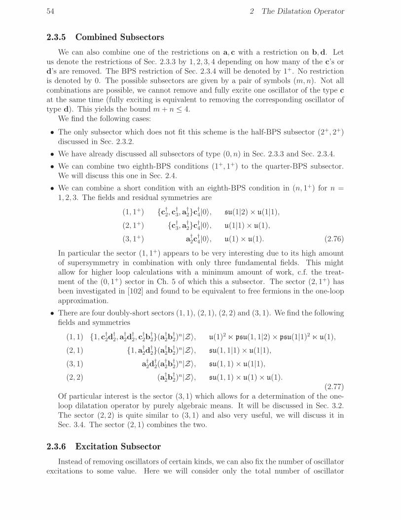
54 2 The Dilatation Operator
2.3.5 Combined Subsectors
We can also combine one of the restrictions on a, c with a restriction on b,d. Letus denote the restrictions of Sec. 2.3.3 by 1, 2, 3, 4 depending on how many of the c’s ord’s are removed. The BPS restriction of Sec. 2.3.4 will be denoted by 1+. No restrictionis denoted by 0. The possible subsectors are given by a pair of symbols (m,n). Not allcombinations are possible, we cannot remove and fully excite one oscillator of the type cat the same time (fully exciting is equivalent to removing the corresponding oscillator oftype d). This yields the bound m+ n ≤ 4.
We find the following cases:
• The only subsector which does not fit this scheme is the half-BPS subsector (2+, 2+)discussed in Sec. 2.3.2.
• We have already discussed all subsectors of type (0, n) in Sec. 2.3.3 and Sec. 2.3.4.
• We can combine two eighth-BPS conditions (1+, 1+) to the quarter-BPS subsector.We will discuss this one in Sec. 2.4.
• We can combine a short condition with an eighth-BPS condition in (n, 1+) for n =1, 2, 3. The fields and residual symmetries are
(1, 1+) {c†2, c†3, a†2}c†4|0〉, su(1|2)× u(1|1),
(2, 1+) {c†3, a†2}c†4|0〉, u(1|1)× u(1),
(3, 1+) a†2c
†4|0〉, u(1)× u(1). (2.76)
In particular the sector (1, 1+) appears to be very interesting due to its high amountof supersymmetry in combination with only three fundamental fields. This mightallow for higher loop calculations with a minimum amount of work, c.f. the treat-ment of the (0, 1+) sector in Ch. 5 of which this a subsector. The sector (2, 1+) hasbeen investigated in [102] and found to be equivalent to free fermions in the one-loopapproximation.
• There are four doubly-short sectors (1, 1), (2, 1), (2, 2) and (3, 1). We find the followingfields and symmetries
(1, 1) {1, c†2d†2, a
†2d
†2, c
†2b
†2}(a†
2b†2)n|Z〉, u(1)2 ⋉ psu(1, 1|2)× psu(1|1)2 ⋉ u(1),
(2, 1) {1, a†2d
†2}(a†
2b†2)n|Z〉, su(1, 1|1)× u(1|1),
(3, 1) a†2d
†2(a
†2b
†2)n|Z〉, su(1, 1)× u(1|1),
(2, 2) (a†2b
†2)n|Z〉, su(1, 1)× u(1)× u(1).
(2.77)Of particular interest is the sector (3, 1) which allows for a determination of the one-loop dilatation operator by purely algebraic means. It will be discussed in Sec. 3.2.The sector (2, 2) is quite similar to (3, 1) and also very useful, we will discuss it inSec. 3.4. The sector (2, 1) combines the two.
2.3.6 Excitation Subsector
Instead of removing oscillators of certain kinds, we can also fix the number of oscillatorexcitations to some value. Here we will consider only the total number of oscillator

2.4 The su(2) Quarter-BPS Sector 55
excitations above the physical vacuum |Z, L〉; this is an even number because oscillatorscan only be excited in pairs due to the central charge constraint. A state with 2Moscillator excitations will be said to have M excitations
‘M excitations ’: (A†)M(A†)M |Z, L〉, (2.78)
where A = (a, c) and A = (b,d). According to Tab. D.2 the excitation number is relatedto the charges by
M = 12(na + nb + nc + nd) = D0 − p− 1
2q1 − 1
2q2, (2.79)
it is thus exactly conserved by the dilatation operator. In other words, the sector of stateswith M excitations is closed. This type of sector is different from the above subsectors inthat no type of oscillator is excluded. Instead, there is an upper bound on the numberof excitations on a single field; this also leads to a simplification of the representation ofgenerators.
The excitation subsectors are somewhat similar to the half-BPS subsector discussedin Sec. 2.3.2, which is in fact the sector with zero excitations. The residual symmetry inthis type of subsector is
(u(1) ⋉ psu(2|2)× psu(2|2) ⋉ u(1)
)× u(1). (2.80)
The generators of psu(2|2) are given by a pair of su(2) generators Lαβ,R
ab and a pair of
supercharges Qaα,S
αa. Classically, they transform between oscillators a and c. Equiva-
lently, the other psu(2|2) is given by Lαβ, R
ab, Q
aα, S
αa. A u(1) external automorphism
for both psu(2|2)’s is given by D0. The u(1) central charge for both psu(2|2)’s is givenby M + δD. Another central charge is δD. The four sets of su(2) generators transformindices canonically. The non-vanishing anticommutators of supergenerators are given by
{Sαa,Q
bβ} = δbaL
αβ + δαβRb
a + 12δbaδ
αβ (M + δD),
{Sαa, Q
bβ} = δbaL
αβ + δα
βRb
a + 12δbaδ
αβ(M + δD). (2.81)
The Dynkin labels of a weight of one of the psu(2|2)’s are given by (i = 1, 2)
[si; ri; qi], ri = 12M + 1
2δD + 1
2si − 1
2qi. (2.82)
For a unitary representation the highest weights should obey ri ≥ si + 1 or si = ri = 0.A multiplet is short for ri = si + 1 and BPS for si = ri = 0. At the unitarity boundri = si + 1, a long multiplet [si; ri; qi] splits off a short multiplet [si − 1; ri − 1; qi + 1] or,when si = 0, a BPS multiplet [0; ri − 1; qi + 2].
A subsector of this kind is suited perfectly to investigate plane-wave physics and BMNoperators [14]. The number of excitations M equals the classical BMN energy D0 − Jor impurity number. The residual symmetry in this sector maps directly to parts of thesymmetries of the dual plane-wave string theory.
2.4 The su(2) Quarter-BPS Sector
In this section we will demonstrate how to extract the dilatation generator from aperturbative calculation of the two-point function. We will restrict to the one-loop leveland to the quarter-BPS subsector.

56 2 The Dilatation Operator
2.4.1 The su(2) Subsector
First of all let us describe the subsector. The quarter-BPS subsector is obtained bycombining both eighth-BPS conditions described in Sec. 2.3.4.
na1= na2
= nb1= nb2
= nc1= nd1
= 0. (2.83)
There are only two charged scalar fields in this subsector
Z := ϕ1 := Φ34 = c†3c†4|0〉 = |Z〉,
φ := ϕ2 := Φ24 = c†2c†4|0〉 = c†2d
†2|Z〉, (2.84)
therefore it is the smallest non-trivial subsector and we will often make use of it. Thepossible weights are
w = (L; 0, 0;K,L− 2K,K; 0, L), (2.85)
where K counts the number of φ’s and L is the total number of fields. The residualsymmetry is
su(2)× u(1)× u(1). (2.86)
The su(2) factor transforms ϕ1 = Z and ϕ2 = φ in the fundamental representation,whereas the u(1)’s measure the classical dimension D0 = L and the anomalous dimensionδD. With respect to su(2)× u(1)× u(1) a state is thus described by the charges
[L− 2K], L, δD, (2.87)
where [L − 2K] is the Dynkin label10 of su(2) corresponding to a third component ofspin L/2−K. In terms of the superconformal algebra, a state with δD = 0 is (at least)quarter-BPS, a generic state, however, will not be protected. In that case the weight wis beyond the unitarity bounds and cannot be primary. The highest weight within thesubsector is obtained from the highest weight of the psu(2, 2|4) multiplet by a shift of
δwI+II = (2; 0, 0; 2, 0, 2; 0, 2). (2.88)
The psu(2, 2|4) highest weight is on both unitarity bounds and has no spin.
2.4.2 Tree-Level
We will now compute the two-point function of states within the su(2) sector. From theformal expression we will then extract the dilatation operator. Let us start at tree-level.The state Oϕ at point x1 is constructed from fields ϕi of the su(2) subsector. Conversely,the other operator Oϕ at point x2 is constructed from fields ϕi of a conjugate su(2)subsector. Note the charge conjugation requires us to use two different su(2) subsectors.The operators are constructed as (not necessarily equal) products of traces of fields
Oϕ[W] = Trϕ∗ · · ·ϕ∗ Trϕ∗ · · ·ϕ∗ . . . , ϕi = ϕi(x1),
Oϕ[W] = Tr ϕ∗ · · · ϕ∗ Tr ϕ∗ · · · ϕ∗ . . . , ϕi = ϕi(x2). (2.89)
10The Dynkin label for su(2) equals twice the spin.

2.4 The su(2) Quarter-BPS Sector 57
Written in this way, the operators become abstract objects in the tensor product space offields and are not necessarily based at some point in spacetime.
According to the path integral (c.f. Sec. 1.2) the two-point function at tree-level isgiven by ⟨
Oϕ Oϕ⟩
= exp(W0[∂/∂W])Oϕ[W] Oϕ[W]∣∣W=0
+O(g). (2.90)
In fact, we do not need to work with generic x-dependent fields W, but only the valuesof the scalar fields ϕ, ϕ at points x1,2 are relevant. The correlator now becomes
⟨Oϕ Oϕ
⟩= exp
(W0(x12, ∂/∂ϕ, ∂/∂ϕ)
)Oϕ(ϕ) Oϕ(ϕ)
∣∣ϕ=ϕ=0
+O(g)
= exp(W0(x12, ϕ, ˇϕ)
)Oϕ Oϕ
∣∣ϕ=ϕ=0
+O(g), (2.91)
where W0 is the free generating functional of connected Graphs
W0(x12, ϕ, ˇϕ) = N−1∆12 Tr ϕi ˇϕi. (2.92)
The scalar propagator ∆12 = ∆(x1, x2) is defined in (2.7). Note that the second line in(2.91) merely involves performing ordinary derivatives ϕ, ˇϕ with respect to the matricesϕ, ϕ. In order for the result to be non-vanishing, all the fields ϕ in Oϕ need to becontracted to fields ϕ in Oϕ with propagators ∆12. In particular, the numbers of fields ofthe two states must be equal.
2.4.3 One-Loop
To compute higher-loop correlators, we insert the interactions Sint[g,W] into the pathintegral
⟨Oϕ Oϕ
⟩= exp(W0[∂/∂W]) exp(−Sint[g,W])Oϕ[W] Oϕ[W]
∣∣W=0
. (2.93)
All the fields W in Sint need to be contracted to propagators before setting W = 0,therefore we can combine the first two exponentials into one and write
⟨Oϕ Oϕ
⟩= exp(W [g, ∂/∂W])Oϕ[W] Oϕ[W]
∣∣W=0
= exp(W (g, x12, ϕ, ˇϕ)
)OϕOϕ
∣∣ϕ=ϕ=0
. (2.94)
Again, it will be sufficient to evaluate the full generating functional of connected graphsW [g,J ] only for fields ϕ, ϕ at points x1,2.
Let us now consider the connected graphs at one-loop. There is no diagram atO(g) which conserves the charges. The O(g2) connected Green functions are depictedin Fig. 2.8. To evaluate them we make use of the regularised N = 4 SYM action in(2.6,1.5). The one-loop Green functions evaluate to
W2,a = 132N−3 X1122 Tr [ˇϕi, ˇϕj ][ϕ
i, ϕj],
W2,b = 132N−3 X1122 Tr [ˇϕi, ϕ
j][ϕi, ˇϕj],
W2,c = 132N−3
(−2H12,12 − 4Y112I12 +X1122
)Tr [ˇϕi, ϕ
i][ ˇϕj , ϕj],
W2,d = −14N−2 Y112 gmn Tr [ˇϕi, tm][tn, ϕ
i] (2.95)

58 2 The Dilatation Operator
a b c d1 d2 d3 d4
Figure 2.8: Connected graphs at one-loop. The solid, wiggly and dashed lines represent scalars,gluons and fermions, respectively. The dotted lines correspond to a non-propagating auxiliaryfield that represents a quartic interaction. The diagrams display the combinatorial structurewith respect to the gauge group rather than their space-time configuration: The white andblack dots are at the spacetime points x1 and x2, respectively.
with the integrals X, Y, H defined in (2.9). We use a Jacobi identity to transform thesecond structure in W2,b
Tr [ˇϕi, ϕj][ϕi, ˇϕj] = Tr [ˇϕi, ˇϕj ][ϕ
i, ϕj]− Tr [ϕi, ˇϕi][ϕj, ˇϕj] (2.96)
and order the terms according to their spacetime integrals
W2,X = 116N−3 X1122 Tr [ˇϕi, ˇϕj ][ϕ
i, ϕj],
W2,H = − 116N−3 H12,12 Tr [ˇϕi, ϕ
i][ˇϕj, ϕj],
W2,IY = −18N−3 I12Y112
(Tr [ˇϕi, ϕ
i][ ˇϕj, ϕj ] +N∆−1
12 gmn Tr [ˇϕi, tm][tn, ϕi]). (2.97)
We refrain from evaluating these functions until later and insert them as they stand intothe expression for the one-loop correlator
⟨Oϕ Oϕ
⟩= exp
(W0(x12, ϕ, ˇϕ)
)(1 + g2W2(x, ϕ, ˇϕ)
)Oϕ Oϕ
∣∣ϕ=ϕ=0
+O(g3). (2.98)
We now change the argument ˇϕ of W2 to N∆−112 ϕ. This can be done because the result
vanishes unless every ϕ is removed by some ϕ before the fields ϕ are set to zero. Here, theonly possibility is to contract with W0 which effectively changes N∆−1
12 ϕ back to ˇϕ. Indoing so we need to make sure that no new contractions appear between the argumentsϕ and ϕ of W2. Formally, this is achieved by ‘normal ordering’. The correlator becomes
⟨Oϕ Oϕ
⟩= exp
(W0(x, ϕ, ˇϕ)
)(1 + g2V2,ϕ(x12)
)Oϕ Oϕ
∣∣ϕ=ϕ=0
+O(g3) (2.99)
with the one-loop effective vertex
V2,ϕ(x12) = :W2(x12, ϕ, N∆−112 ϕ):. (2.100)
We transform the explicit expressions for the connected graphs (2.97) and obtain
V2,X = 14N−1 X1122I
−212 :Tr [ϕi, ϕj][ϕ
i, ϕj]:,
V2,H = −14N−1 H12,12I
−212 :Tr [ϕi, ϕ
i][ϕj, ϕj]:,
V2,IY = −12N−1Y112I
−112
(:Tr [ϕi, ϕ
i][ϕj , ϕj]: + gmn:Tr [ϕi, tm][tn, ϕ
i]:). (2.101)
We can change the normal ordering in the first term of V2,IY in order to absorb the second,see (1.41)
V2,IY = −12N−1Y112I
−112 Tr:[ϕi, ϕ
i]::[ϕj , ϕj]: = 1
2N−1Y112I
−112 Tr jj. (2.102)

2.4 The su(2) Quarter-BPS Sector 59
We can thus write V2,IY in terms of the generator of gauge rotations j = i:[ϕi, ϕi]: within
the su(2) subsector, see (1.37). Therefore V2,IY does not act on gauge invariant objectssuch as the states O and we can drop it altogether, V2,IY = 0.
Instead of replacing ˇϕ we could also have replaced ϕ resulting in the effective vertex
V2,ϕ(x12) = :W2(x12, N∆−112 ϕ, ˇϕ):. (2.103)
This shows that in (2.99) V2,ϕ is equivalent to V2,ϕ
V2,ϕ = V2,ϕ. (2.104)
The form of this V2,ϕ is the same as in (2.101) upon conjugation of su(2) indices. In otherwords, V2 is self-adjoint with respect to the tree-level scalar product.
In a renormalised theory we should compute the correlator of renormalised states ZO.At this point it is possible to guess the operator Z for the renormalisation of states
Z = 1− 12g2V2(1/µ) +O(g3). (2.105)
We insert this into (2.99) and use the equivalence of V2,ϕ and V2,ϕ to find
⟨ZOϕ ZOϕ
⟩= exp
(W0(x12, ϕ, ˇϕ)
)(1 + g2V2,ϕ(x12)− g2V2,ϕ(1/µ)
)Oϕ Oϕ
∣∣ϕ=ϕ=0
+O(g3).
(2.106)A closer look at V2(x12) reveals that the x12-dependence is only through ξ as definedin (2.11). This is a manifest property of a renormalisable field theory in dimensionalregularisation. We can thus write
V2(x12) = ξV2 =Γ(1− ǫ)∣∣12µ2x2
12
∣∣−ǫ V2. (2.107)
We send the regulator to zero and find
limǫ→0
(V2(x12)− V2(1/µ)
)= log |µx12|−2D2 (2.108)
withD2 = − lim
ǫ→0ǫV2. (2.109)
In the case at hand, we obtain from (2.101)
D2 = −12N−1:Tr [φi, φj][φ
i, φj]:, (2.110)
where we have used the following expansion in ǫ, see (2.10), for the functions appearingin V2
X00xxI−20x ξ
−1 = 2ǫ−1 + 2 +O(ǫ2),
H0x,0xI−20x ξ
−1 = −48ζ(3) ǫ+O(ǫ2). (2.111)
The final answer for the renormalised correlator at ǫ = 0 is
⟨ZOϕ ZOϕ
⟩= exp(W0) exp
(log |µx12|−2g2D2,ϕ
)Oϕ Oϕ
∣∣ϕ=ϕ=0
+O(g3), (2.112)

60 2 The Dilatation Operator
in agreement with the form predicted by conformal field theory.11 The operator D2
is the one-loop correction to the dilatation generator. Furthermore, the coefficient ofthe correlator is given by its tree-level value. Notice that although we are interested incorrelators of renormalised operators ZO as on the left-hand side of (2.112), we can workwith bare operators O as on the right hand side of (2.112). In other words, we choose torenormalise the dilatation operator instead of the states.
2.4.4 Application
In the last section we have derived the one-loop dilatation generator (2.110) for thesu(2) subsector. When we write it in components (Z, φ) = (ϕ1, ϕ2) it reads
D2 = −N−1:Tr [Z, φ][Z, φ]:. (2.113)
Using the rules in Sec. 1.5 we can determine its action on any operator of the formTrZZφZφTrφ . . . .
Let us now apply D2 to rederive the results of Sec. 2.1.1. The first observation isthat D2 acts on Z and φ simultaneously. If either of them is absent in the state, D2 willannihilate it, therefore
D2 TrZ · · ·Z TrZ · · ·Z . . . = 0. (2.114)
As emphasised in Sec. 2.3.2, these states are half-BPS and thus protected from quantumcorrections. In particular, the operator Qmn has one component, TrZZ, of this type.The other state discussed in Sec. 2.1, the Konishi operator K, is not part of the su(2)sector. However, it is on both unitarity bounds and has spin zero. Therefore, it has adescendant within the subsector whose weight is given by (2.13,2.88)
w′K = wK + δwI+II = (4; 0, 0; 2, 0, 2; 0, 4). (2.115)
This is a state of length L = 4 with K = 2 fields of type φ, see also [41]. Let us writedown a basis for all such states in SU(N) gauge theory (the line separates single fromdouble-trace states)
ET =
TrZZφφTrZφZφ
TrZZ TrφφTrZφ TrZφ
. (2.116)
We apply the one-loop dilatation operator to the basis, D2E = ED2, and obtain thematrix of anomalous dimensions
D2 =
+2 −4 + 8N− 4N
−2 +4 − 8N
+ 4N
0 0 0 00 0 0 0
. (2.117)
Its eigenvectors are
(−2, 2, 0, 0)T, (2, 1, 0, 0)T, (0, 0, 1, 2)T, (− 2N, 2N, 1,−1)T. (2.118)
11In fact, the mass dimension of the operators has not changed from its classical value, hence theresidual µ-dependence. The fully renormalised operator to be inserted into the path integral would beµδD(g)ZO, but formally this cannot be expanded into a series as emphasised above.

2.5 Field Theoretic Considerations 61
The first one corresponds to the Konishi descendant
K′ = −2 TrZφZφ+ 2 TrZφφZ = Tr [Z, φ][Z, φ], D(g) = 2 + 6g2 +O(g3) (2.119)
with eigenvalue D2 = 6. The other three states have vanishing anomalous dimension.The first two, 2 TrZZφφ + TrZφZφ and TrZZ Trφφ + 2 TrZφTrZφ are related toTrZZZZ and TrZZ TrZZ by su(2) rotations; this explains D2 = 0. The last operator
O = TrZZ Trφφ− TrZφTrZφ+N−1 Tr [Z, φ][Z, φ], D2 = 0 (2.120)
is indeed a highest weight state of psu(2, 2|4), as such it is, unlike K′, quarter-BPS andprotected [41, 42, 34].
2.5 Field Theoretic Considerations
In this section we will investigate the structure of the dilatation operator at higherorders in perturbation theory without actually computing it. This will yield importantstructural constraints for the algebraic construction pursued in the following chapters.
2.5.1 Two-Point Functions at Higher-Loops
Here, we would like to continue the investigation of the last section at higher loopsand see how the dilatation operator can be extracted. We will show how to resolve somecomplications which appear starting at four loops and which are due to the fact that thevarious loop contributions to the dilatation operator do not commute with each other,e.g. [D2,D4] 6= 0. We will not compute higher-loop amplitudes explicitly.
To obtain the arbitrary loop correlator we insert all ℓ-loop connected Green functionsW2ℓ in the correlator
⟨Oϕ Oϕ
⟩= exp(W0) exp
(∑∞ℓ=1g
2ℓW2ℓ(x12, ϕ, ˇϕ))Oϕ Oϕ
∣∣ϕ=ϕ=0
. (2.121)
In analogy to (2.99) we change the argument ˇϕ of W2ℓ(x, ϕ, ˇϕ) to N∆−112 ϕ
⟨Oϕ Oϕ
⟩= exp(W0) :exp
(∑∞ℓ=1g
2ℓW2ℓ(x12, ϕ, N∆−112 ϕ)
):Oϕ Oϕ
∣∣ϕ=ϕ=0
. (2.122)
Alternatively, we could change the argument ϕ to N∆−112 ϕ. We would then like to rewrite
(2.122) in a convenient form for the conformal structure of the correlator:
⟨Oϕ Oϕ
⟩= exp(W0) exp
(Vϕ(x12)
)Oϕ Oϕ
∣∣ϕ=ϕ=0
= exp(W0) exp(Vϕ(x12)
)Oϕ Oϕ
∣∣ϕ=ϕ=0
, (2.123)
where12
V (x12) =∞∑
ℓ=1
g2ℓV2ℓ(x12)− 148g8[V2(x12), [V2(x12), V4(x12)]
]+ . . . . (2.124)
12The commutator term was included for convenience, it could have been included in V8, we will explainthis issue below.
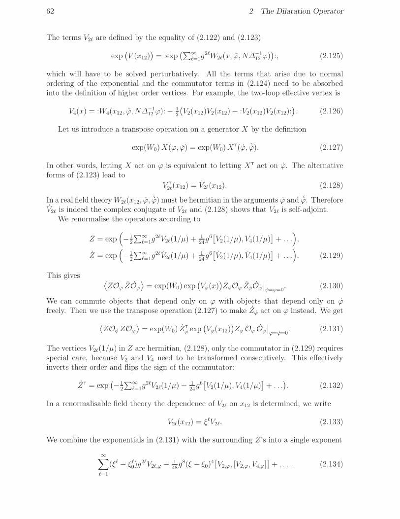
62 2 The Dilatation Operator
The terms V2ℓ are defined by the equality of (2.122) and (2.123)
exp(V (x12)
)= :exp
(∑∞ℓ=1g
2ℓW2ℓ(x, ϕ, N∆−112 ϕ)
):, (2.125)
which will have to be solved perturbatively. All the terms that arise due to normalordering of the exponential and the commutator terms in (2.124) need to be absorbedinto the definition of higher order vertices. For example, the two-loop effective vertex is
V4(x) = :W4(x12, ϕ, N∆−112 ϕ):− 1
2
(V2(x12)V2(x12)− :V2(x12)V2(x12):
). (2.126)
Let us introduce a transpose operation on a generator X by the definition
exp(W0)X(ϕ, ϕ) = exp(W0)XT(ϕ, ˇϕ). (2.127)
In other words, letting X act on ϕ is equivalent to letting XT act on ϕ. The alternativeforms of (2.123) lead to
V T
2ℓ(x12) = V2ℓ(x12). (2.128)
In a real field theoryW2ℓ(x12, ϕ, ˇϕ) must be hermitian in the arguments ϕ and ˇϕ. ThereforeV2ℓ is indeed the complex conjugate of V2ℓ and (2.128) shows that V2ℓ is self-adjoint.
We renormalise the operators according to
Z = exp(−1
2
∑∞ℓ=1g
2ℓV2ℓ(1/µ) + 124g6[V2(1/µ), V4(1/µ)
]+ . . .
),
Z = exp(−1
2
∑∞ℓ=1g
2ℓV2ℓ(1/µ) + 124g6[V2(1/µ), V4(1/µ)
]+ . . .
). (2.129)
This gives ⟨ZOϕ ZOϕ
⟩= exp(W0) exp
(Vϕ(x)
)ZϕOϕ ZϕOϕ
∣∣φ=ϕ=0
. (2.130)
We can commute objects that depend only on ϕ with objects that depend only on ϕfreely. Then we use the transpose operation (2.127) to make Zϕ act on ϕ instead. We get
⟨ZOφZOϕ
⟩= exp(W0) Z
T
ϕ exp(Vϕ(x12)
)ZϕOϕ Oϕ
∣∣ϕ=ϕ=0
. (2.131)
The vertices V2ℓ(1/µ) in Z are hermitian, (2.128), only the commutator in (2.129) requiresspecial care, because V2 and V4 need to be transformed consecutively. This effectivelyinverts their order and flips the sign of the commutator:
ZT = exp(−1
2
∑∞ℓ=1g
2ℓV2ℓ(1/µ)− 124g6[V2(1/µ), V4(1/µ)
]+ . . .
). (2.132)
In a renormalisable field theory the dependence of V2ℓ on x12 is determined, we write
V2ℓ(x12) = ξℓV2ℓ. (2.133)
We combine the exponentials in (2.131) with the surrounding Z’s into a single exponent
∞∑
ℓ=1
(ξℓ − ξℓ0)g2ℓV2ℓ,ϕ − 148g8(ξ − ξ0)4
[V2,ϕ, [V2,ϕ, V4,ϕ]
]+ . . . . (2.134)

2.5 Field Theoretic Considerations 63
The ℓ-loop Green function W2ℓ is expected to have multiple poles at ǫ = 0. In a conformalfield theory, however, these poles must have cancelled in the combination V2ℓ as given by(2.124,2.125). If so, we can finally send the regulator to zero and find
⟨ZOϕ ZOϕ
⟩= exp(W0) exp
(log |µx12|−2∑∞
ℓ=1g2ℓD2ℓ,ϕ
)Oϕ Oϕ
∣∣ϕ=ϕ=0
(2.135)
with
D2ℓ = −ℓ limǫ→0
ǫV2ℓ. (2.136)
Note that the commutator term in (2.134) vanishes due to four powers of ǫ from (ξ− ξ0)4
as opposed to only three powers of 1/ǫ from the V2ℓ. For this cancellation to happen thecommutator terms in (2.124) and (2.129) are necessary: We have investigated all possibleterms that can arise in a four-loop computation. We find that precisely the commutatorstructure in (2.124) is required to obtain a finite, conformally covariant correlator.
Some comments about the renormalisation programme are in order. Firstly, the pro-gramme ensures that the coefficient of the two-point function is given by free contractionsof the unrenormalised operators. Secondly, the effective vertices V2ℓ are self-adjoint withrespect to the scalar product induced by free contractions, see (2.128). The same holdsfor the dilatation generator which consequently has real eigenvalues. Notice that in somecase there may appear to be complex eigenvalues. However, a more careful analysis willshow that the corresponding eigenstate is zero. This may happen if the rank of the groupis small compared to the size of the operators and group identities lead to non-triviallinear dependencies in the basis of operators.
2.5.2 Two-Point Functions of Non-Scalar Operators
Correlation functions of non-scalar operators are not as easy to handle as their scalarcounterparts. This is due to their spacetime indices which can not only be contractedamong themselves but also with x12. Furthermore, there are qualitative differences be-tween primaries and descendants, see Sec. 1.10. Therefore the form predicted by conformalsymmetry is not as simple as (2.135). It certainly involves the symmetry generators K
and P to be able to distinguish between primaries and descendants. These generatorsalso receive quantum corrections, which would have to be found at the same time.
However, in some cases the dilatation generator may be obtained anyway withouttaking these complications into account. A crucial observation is that, although (1.93)and (1.96) are different, the difference is only in the part that multiplies xµ12x
ν12. The
‘direct’ contraction via ηµν is the same for both. If all contractions between the operatorindices and x12 are dropped, the operators behave as though they were a set of scalars.In [50] this simplification made a computation of the one-loop dilatation operator possiblewithin the non-scalar subsector (2, 2).
Note that the covariant derivatives acting on a field are just ordinary partial deriva-tives at leading order. The appearance of the gauge connection should be treated as aninteraction that takes place at the point of the field (boundary) and everywhere in space-time (bulk). Algebraically, the structure of boundary interactions is the same as in thebulk, the gauge field couples to the field via the gauge group structure constants and onepower of the coupling constant.
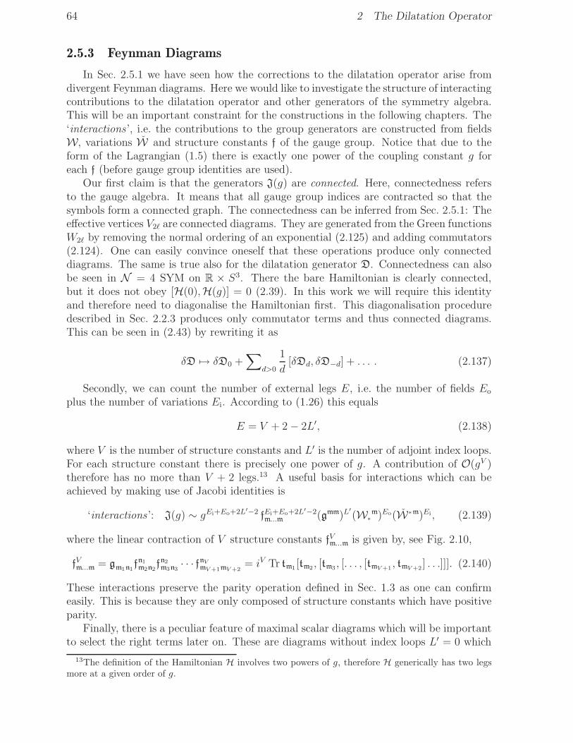
64 2 The Dilatation Operator
2.5.3 Feynman Diagrams
In Sec. 2.5.1 we have seen how the corrections to the dilatation operator arise fromdivergent Feynman diagrams. Here we would like to investigate the structure of interactingcontributions to the dilatation operator and other generators of the symmetry algebra.This will be an important constraint for the constructions in the following chapters. The‘interactions’, i.e. the contributions to the group generators are constructed from fieldsW, variations W and structure constants f of the gauge group. Notice that due to theform of the Lagrangian (1.5) there is exactly one power of the coupling constant g foreach f (before gauge group identities are used).
Our first claim is that the generators J(g) are connected. Here, connectedness refersto the gauge algebra. It means that all gauge group indices are contracted so that thesymbols form a connected graph. The connectedness can be inferred from Sec. 2.5.1: Theeffective vertices V2ℓ are connected diagrams. They are generated from the Green functionsW2ℓ by removing the normal ordering of an exponential (2.125) and adding commutators(2.124). One can easily convince oneself that these operations produce only connecteddiagrams. The same is true also for the dilatation generator D. Connectedness can alsobe seen in N = 4 SYM on R × S3. There the bare Hamiltonian is clearly connected,but it does not obey [H(0),H(g)] = 0 (2.39). In this work we will require this identityand therefore need to diagonalise the Hamiltonian first. This diagonalisation proceduredescribed in Sec. 2.2.3 produces only commutator terms and thus connected diagrams.This can be seen in (2.43) by rewriting it as
δD 7→ δD0 +∑
d>0
1
d[δDd, δD−d] + . . . . (2.137)
Secondly, we can count the number of external legs E, i.e. the number of fields Eo
plus the number of variations Ei. According to (1.26) this equals
E = V + 2− 2L′, (2.138)
where V is the number of structure constants and L′ is the number of adjoint index loops.For each structure constant there is precisely one power of g. A contribution of O(gV )therefore has no more than V + 2 legs.13 A useful basis for interactions which can beachieved by making use of Jacobi identities is
‘interactions’: J(g) ∼ gEi+Eo+2L′−2 fEi+Eo+2L′−2m...m (gmm)L
′
(W∗
m)Eo(W∗m)Ei, (2.139)
where the linear contraction of V structure constants fVm...m is given by, see Fig. 2.10,
fVm...m = gm1n1fn1
m2n2fn2
m3n3· · · fnV
mV +1mV +2= iV Tr tm1
[tm2, [tm3
, [. . . , [tmV +1, tmV +2
] . . .]]]. (2.140)
These interactions preserve the parity operation defined in Sec. 1.3 as one can confirmeasily. This is because they are only composed of structure constants which have positiveparity.
Finally, there is a peculiar feature of maximal scalar diagrams which will be importantto select the right terms later on. These are diagrams without index loops L′ = 0 which
13The definition of the Hamiltonian H involves two powers of g, therefore H generically has two legsmore at a given order of g.

2.6 The Planar Limit and Spin Chains 65
gf
gf
gf
gf
gf
gf
gf
gf
gf
gf
gf
gf
gf
W∗W∗W∗W∗
W∗W∗W∗ W∗W∗
Figure 2.10: A generic interaction with Ei = 5 variations, Eo = 4 fields, L′ = 3 index loops andV = 13 structure constants and powers of the coupling constant.
therefore have the maximum number of external scalar legs V +2 at order V in perturba-tion theory. We are interested in the flow of so(6) vector indices across the diagram. Asthis is a tree diagram, the internal lines can only be scalars or gauge fields. Gauge fieldsare singlets of so(6) therefore only scalar fields can support the flow. Only at quarticinteractions of the scalars two lines of flow can cross. This shows that at order V therecannot be more than V/2 crossings of so(6) vector flow lines.
2.6 The Planar Limit and Spin Chains
Generic interactions have a very complicated structure due to a large number of pos-sible contractions between the indices in (2.139). Most of the time it is therefore usefulto restrict to the planar limit, see Sec. 1.4.
2.6.1 States
In the large N limit, field theory diagrams are suppressed unless 2C−2G−T = 0, see(1.44). As each component requires at least two traces, one incoming and one outgoing(there are no vacuum diagrams), we need T = 2C andG = 0. In other words, the diagramsmay connect only two single trace operators and cannot have handles. Therefore it makessense to consider only single trace states
‘single-trace state’: |A1 . . .AL〉 := TrWA1· · ·WAL
. (2.141)
The cyclicity of the trace gives rise to cyclic identifications
|A1 . . .ApAp+1 . . .AL〉 = (−1)(A1...Ap)(Ap+1...AL)|Ap+1 . . .ALA1 . . .Ap〉. (2.142)
The sign is due to statistics of the fields: (−1)XY equals −1 if both, X and Y , are fermionicand +1 otherwise. In particular, some states are incompatible with this symmetry
|A1 . . .AL/2A1 . . .AL/2〉 = 0, if A1 . . .AL/2 is fermionic. (2.143)
A generic state is a linear superposition of the above basis states
O = c |A1 . . .AL〉+ c′ |A′1 . . .A′
L′〉+ . . . , (2.144)
where mixing of states with different length is explicitly allowed.

66 2 The Dilatation Operator
B1 B2B3
Cp+5A1 A2 A3 A4Cp
{A1...A4
B1...B3
}
O
Figure 2.12: Insertion of a planar interaction. The black dots correspond to fields, the whitedots to variations. Inside the blob there is some unspecified planar diagram that connects thedots.
2.6.2 Interactions
For planar interactions the precise structure of internal connections does not play arole as long as it is planar, c.f. Fig. 2.12. The only relevant structure is the order ofexternal legs. In the planar limit it is therefore sufficient to consider interactions of thetype
‘planar interactions’:{A1...AEi
B1...BEo
}:= N1−Ei TrWB1
. . .WBEoWAEi . . . WA1 , (2.145)
which searches for the sequence of fields WA1. . .WAEi
within a state and replaces it bythe sequence WB1
. . .WBEo. More explicitly, the action on a state |C1 . . . CL〉 is
L∑
p=1
(−1)(C1...Cp−1)(B1...BEoA1...AEi)δA1
Cp. . . δ
AEi
Cp+Ei−1|C1 . . . Cp−1B1 . . .BEo
Cp+Ei. . . CL〉. (2.146)
A sample action is{AB
BA}|12345〉 = |21345〉 ± |13245〉 ± |12435〉 ± |12354〉 ± |52341〉. (2.147)
The order of an interaction in perturbation theory is given by V = Ei +Eo + 2L′− 2,therefore J(g) ∼ gEi+Eo+2L′−2
{A1...AEi
B1...BEo
}. We see that for planar interactions, adding an
index loop simply increases the loop order by one. At a fixed loop order this leads todiagrams with fewer external legs. To reduce the complexity, we can install a pair of legsby means of a gauge transformation. For that purpose we insert the generator of gaugerotations j into some interaction
0 = −iTr j WB1. . .WBEo
WAEi . . . WA1
= Tr:WCWC:WB1. . .WBEo
WAEi . . . WA1 − Tr:WCWC:WB1. . .WBEo
WAEi . . . WA1
= N TrWB1. . .WBEo
WAEi . . . WA1 ∓ TrWCWB1. . .WBEo
WAEi . . . WA1WC. (2.148)
The equivalence in the last line is for planar insertions only. This means that adding apair of legs to the left of the interaction has no effect. Equivalently, we can add a pair oflegs to the right of the interaction
{A1...AEi
B1...BEo
}={A1...AEi
CB1...BEoC
}= (−1)C(A1...AEi
B1...BEo ){CA1...AEi
CB1...BEo
}. (2.149)

2.6 The Planar Limit and Spin Chains 67
[A1...A5
B1...B6
]
O B1
B2B3
B4
B5 B6
A1
A2
A3
A4
A5
Figure 2.14: The action of a wrapping interaction. For a planar insertion, the wrapping interac-tion must surround the state and the number of fields L must match the number of variationsEi.
This is obvious because the additional pair of legs does not change the field at thatposition, it is only a spectator. We can now add L′ pairs of spectator legs to an interactionand thus drop the index loop parameter14
Jk ∼{A1...AEi
B1...BEo
}, with Ei + Eo = k + 2. (2.150)
2.6.3 Wrapping Interactions
This can, however, not be completely true: If the number of variations, Ei, equals thelength of the state, L, we cannot add a spectator pair of legs. In fact, there is a subtletyin the second equivalence in (2.148): When in the second term the variation hits the fieldWBEo
we get a ‘wrapping diagram’. It can be represented by the following symbol andtrace structure
‘wrapping interactions’:[A1...AEi
B1...BEo
]:= N−Ei TrWB1
. . .WBEoTr WAEi . . . WA1 . (2.151)
Wrapping interactions remove the state as a whole and replace it by a new one. Theyare best understood graphically, see Fig. 2.14. Wrapping diagrams are generically non-planar, but when applied to a state of the minimally required length, the action becomesplanar. This is because the diagram can be wrapped fully around the trace. If, however,some uncontracted fields remain within the trace, they are disconnected from the fields ofthe interaction and the action is non-planar. An improved version of (2.149) which takesstates of finite length into account is
{A1...AEi
B1...BEo
}={A1...AEi
CB1...BEoC
}+[A1...AEi
B1...BEo
]= (−1)C(A1...AEi
B1...BEo ){CA1...AEi
CB1...BEo
}+[A1...AEi
B1...BEo
](2.152)
For wrapping diagrams the order in perturbation theory is given by
Jk ∼[A1...AEi
B1...BEo
]with Ei + Eo = k + 2− 2L′, L′ ≥ 1. (2.153)
They act only on states with length L = Ei and need at least one index loop L′. Thereforethey appear only at rather high loop orders, especially for long states. Unfortunately,
14Note that for Hk as defined in Sec. 2.2.4 there should be Ei + Eo = k + 4 legs.
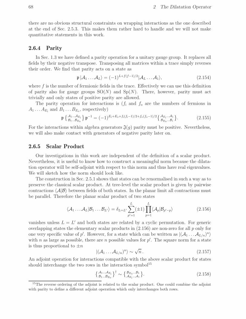
68 2 The Dilatation Operator
there are no obvious structural constraints on wrapping interactions as the one describedat the end of Sec. 2.5.3. This makes them rather hard to handle and we will not makequantitative statements in this work.
2.6.4 Parity
In Sec. 1.3 we have defined a parity operation for a unitary gauge group. It replaces allfields by their negative transpose. Transposing all matrices within a trace simply reversestheir order. We find that parity acts on a state as
p |A1 . . .AL〉 = (−1)L+f(f−1)/2|AL . . .A1〉, (2.154)
where f is the number of fermionic fields in the trace. Effectively we can use this definitionof parity also for gauge groups SO(N) and Sp(N). There, however, parity must acttrivially and only states of positive parity are allowed.
The parity operation for interactions is (fi and fo are the numbers of fermions inA1 . . . AEi
and B1 . . . BEo, respectively)
p{A1...AEi
B1...BEo
}p−1 = (−1)Ei+Eo+fi(fi−1)/2+fo(fo−1)/2
{AEi...A1
BEo ...Bi
}. (2.155)
For the interactions within algebra generators J(g) parity must be positive. Nevertheless,we will also make contact with generators of negative parity later on.
2.6.5 Scalar Product
Our investigations in this work are independent of the definition of a scalar product.Nevertheless, it is useful to know how to construct a meaningful norm because the dilata-tion operator will be self-adjoint with respect to this norm and thus have real eigenvalues.We will sketch how the norm should look like.
The construction in Sec. 2.5.1 shows that states can be renormalised in such a way as topreserve the classical scalar product. At tree-level the scalar product is given by pairwisecontractions 〈A|B〉 between fields of both states. In the planar limit all contractions mustbe parallel. Therefore the planar scalar product of two states
〈A1 . . .AL|B1 . . .BL′〉 = δL=L′
L∑
p′=1
(±1)L∏
p=1
〈Ap|Bp′−p〉 (2.156)
vanishes unless L = L′ and both states are related by a cyclic permutation. For genericoverlapping states the elementary scalar products in (2.156) are non-zero for all p only forone very specific value of p′. However, for a state which can be written as |(A1 . . .AL/n)n〉with n as large as possible, there are n possible values for p′. The square norm for a stateis thus proportional to ±n
|(A1 . . .AL/n)n〉 ∼√n . (2.157)
An adjoint operation for interactions compatible with the above scalar product for statesshould interchange the two rows in the interaction symbol15
{A1...AEi
B1...BEo
}† ∼{ BEo ...B1
AEi...A1
}. (2.158)
15The reverse ordering of the adjoint is related to the scalar product. One could combine the adjointwith parity to define a different adjoint operation which only interchanges both rows.

2.6 The Planar Limit and Spin Chains 69
A1
A2A3
A4A5A6
A7
A8 A9 A10A11A12
Figure 2.16: A single-trace operator as a spin chain. For the simplest spin chain, the spin cantake two alignments, for N = 4 the ‘spin’ can take infinitely many.
planar N = 4 SYM psu(2, 2|4) spin chainsingle trace operator cyclic spin chainfield spin siteanomalous dilatation operator g−2δD Hamiltonian Hanomalous dimension g−2δD energy Ecyclicity constraint zero-momentum condition U = 1
Table 2.2: Dictionary for N = 4 SYM and the spin chain picture.
Note, however, that the action of a self-adjoint interaction on a set of states is onlyequivalent to a hermitian matrix if all states are normalised to one with respect to (2.157).Otherwise the matrix is only self-adjoint with respect to the norm on the set of states.For example, this is the case for the asymmetric matrix (2.117).
2.6.6 Spin Chains
Single-trace local operators can be viewed as states of a dynamic, cyclic, quantum spinchain [48]. A cyclic spin chain is a set of L spin sites with a cyclic adjacency property. Ina quantum spin chain, the spin at each site is a module of the symmetry algebra of thesystem and the Hilbert space is the tensor product of L spin modules. For a dynamic spinchain the number of sites L is not fixed [51]; the full Hilbert space is the tensor product ofall Hilbert spaces of a fixed length. The basic quantum spin chain is the Heisenberg chain.Its symmetry group is su(2) and all spins transform in the fundamental representation.A basis for the Hilbert space is given by those states for which the spin at each site pointseither ‘up’ or ‘down’. The Hilbert space is thus C
2L
. In a more general spin chain, the spincan point in more than just two directions, in most cases even infinitely many. Note thatthe cyclic identification (2.142) of field theory states is an additional constraint on cyclicspin chains. For example, the field theory Hilbert space corresponding to the Heisenbergchain is C2L
/ZL. Physical states are identified by a trivial shift operator, states withnon-zero momentum are unphysical.
In the spin chain picture each field is identified with one site of the chain. Thealignment of the spin at that site corresponds to the component of the multiplet of fields,c.f. Fig. 2.16. For N = 4 SYM, the spin chain is a psu(2, 2|4) cyclic super spin chain withspins transforming in the representation [0; 0; 0, 1, 0; 0; 0], see Sec. 1.9, [58]. When workingin the planar limit, we will commonly make use of spin chain terminology. In particular,the quantum correction to the dilatation generator will be called the ‘Hamiltonian’ H =g−2δD and anomalous dimensions are synonymous for ‘energies’ E = g−2δD, see Tab. 2.2for a small dictionary. For the other generators of the superconformal group we use thesame symbols as in the non-planar case.

70
71
Chapter 3
One-Loop
In this chapter we will derive the complete one-loop dilatation operator ofN = 4 SuperYang-Mills Theory. The text is based on the article [50], but we present a new derivationof the coefficients Cj. In [50] the coefficients have been obtained in a quantum fieldtheory calculation, here we will merely employ the superconformal algebra. The spectraland plane-wave investigations have been compiled from the articles [35, 27, 38, 50, 103].
3.1 The Form of the Dilatation Generator
We start by investigating the general form of the one-loop dilatation generator. We willsee that representation theory of the symmetry group as well as Feynman diagrammaticsput tight constraints on the form. What remains is a sequence of undetermined coefficientsCj, one for each value of ‘total spin’.
3.1.1 One-Loop as Leading Order
In Sec. 2.2.4 we have learned that the leading order anomalous dilatation operatorDl isinvariant under classical superconformal transformations J0. It is impossible to constructan invariant operator D1 at first order of the coupling constant g, therefore the leadingorder is one-loop, l = 2. We will come back to this point after having reviewed somerepresentation theory at the end of Sec. 3.1.3. In what follows we will consider only theclassical psu(2, 2|4) algebra of generators J0; the one-loop anomalous dilatation generatorD2 will be considered an independent object; we will refer to it as the Hamiltonian H,
J(g) = J +O(g), D(g) = D + g2H +O(g3), [J,H] = 0. (3.1)
3.1.2 Generic Form
The Hamiltonian has the following generic form1
H = −N−1(Ca)AB
CD:Tr[WA, WC
][WB, WD
]:
−N−1(Cb)AB
CD:Tr[WA,WB
][WC, WD
]:
+N−1(Cc)A
Bgmn:Tr
[WA, tm
][tn, WB
]:. (3.2)
1These expressions are valid for bosonic fields WA only. They do generalise to fermions, but only atthe cost of obscure signs at various places.
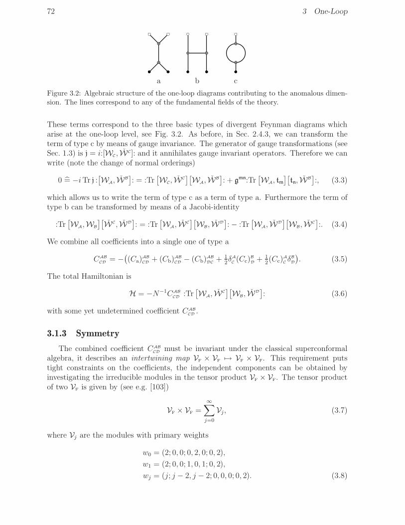
72 3 One-Loop
a b c
Figure 3.2: Algebraic structure of the one-loop diagrams contributing to the anomalous dimen-sion. The lines correspond to any of the fundamental fields of the theory.
These terms correspond to the three basic types of divergent Feynman diagrams whicharise at the one-loop level, see Fig. 3.2. As before, in Sec. 2.4.3, we can transform theterm of type c by means of gauge invariance. The generator of gauge transformations (seeSec. 1.3) is j = i:[WC, WC]: and it annihilates gauge invariant operators. Therefore we canwrite (note the change of normal orderings)
0 = −iTr j :[WA, WB
]: = :Tr
[WC, WC
][WA, WB
]: + gmn:Tr
[WA, tm
][tn, WB
]:, (3.3)
which allows us to write the term of type c as a term of type a. Furthermore the term oftype b can be transformed by means of a Jacobi-identity
:Tr[WA,WB
][WC, WD
]: = :Tr
[WA, WC
][WB, WD
]:− :Tr
[WA, WD
][WB, WC
]:. (3.4)
We combine all coefficients into a single one of type a
CAB
CD= −
((Ca)
AB
CD+ (Cb)
AB
CD− (Cb)
AB
DC+ 1
2δA
C(Cc)
B
D+ 1
2(Cc)
A
CδB
D
). (3.5)
The total Hamiltonian is
H = −N−1CAB
CD:Tr[WA, WC
][WB, WD
]: (3.6)
with some yet undetermined coefficient CAB
CD.
3.1.3 Symmetry
The combined coefficient CAB
CDmust be invariant under the classical superconformal
algebra, it describes an intertwining map VF × VF 7→ VF × VF. This requirement putstight constraints on the coefficients, the independent components can be obtained byinvestigating the irreducible modules in the tensor product VF × VF. The tensor productof two VF is given by (see e.g. [103])
VF × VF =∞∑
j=0
Vj, (3.7)
where Vj are the modules with primary weights
w0 = (2; 0, 0; 0, 2, 0; 0, 2),
w1 = (2; 0, 0; 1, 0, 1; 0, 2),
wj = (j; j − 2, j − 2; 0, 0, 0; 0, 2). (3.8)

3.1 The Form of the Dilatation Generator 73
The module V0 is the half-BPS current multiplet, V1 is quarter-BPS and the other ones aredoubly-short. As an aside, it is interesting to see that the quadratic Casimir (c.f. App. D.3)for these modules is given by
J212 Vj = j(j + 1)Vj, (3.9)
just as if we were dealing with sl(2) alone. Due to invariance, CAB
CDmust be of block-
diagonal form: All states of a module Vj must be mapped to the same type of moduleVj with equal coefficients. In our case, each module Vj appears only once in the tensorproduct, therefore we can assign only one coefficient Cj for each Vj . Let (Pj)AB
CDproject
two fields WA,WB to the module Vj. Then the most general invariant coefficients can bewritten as
CAB
CD=
∞∑
j=0
Cj (Pj)AB
CD. (3.10)
Note that the decomposition (3.7) is also valid for the group pu(2, 2|4). Therefore, thehypercharge B is preserved by H. Obviously, also the length, measured by the operatorL, is conserved
[H,B] = [H,L] = 0. (3.11)
This will clearly not be the case for higher-loop corrections to the dilatation genera-tor, which act on more than two fields at the same time. At higher loops, the Konishianomaly [104] mixes operators of different hypercharges. The same points also hold forthe length L of a state. Nevertheless, it makes perfect sense to speak of the leading orderhypercharge and length to describe a state. Mixing with states of different hyperchargesor lengths is sub-leading, because the one-loop dilatation generator conserves these.
At this point we can also exclude the possibility of a ‘half-loop’ contribution D1 ora length non-preserving contribution to D2 on algebraic grounds: There is no overlapbetween the irreducible modules in the in and out channels
V0F6∈ V3
F, VF 6∈ V2
F, V0
F6∈ V4
F, VF 6∈ V3
F, (3.12)
which can be seen by comparing the scaling dimensions. The only possible contributionsup to second order in g are V2
F7→ V2
For VF 7→ VF as assumed in (3.2).
3.1.4 Planar Limit
We can now take the planar limit of (3.6)
H =∞∑
j=0
2Cj (Pj)AB
CD
{ CDAB}
(3.13)
in the notation introduced in Sec. 2.6.2. In this chapter we will use a slightly differentnotation which assumes that H acts on a spin chain of length L and transforms twoadjacent fields2
H =L∑
p=1
Hp,p+1, Hp,p+1 =∞∑
j=0
2CjPp,p+1,j. (3.14)
2We assume cyclic site indices, i.e. HL,L+1 = HL,1.

74 3 One-Loop
The symbol Pp,p+1,j projects the fields at positions p, p + 1 to the module Vj . We seethat all coefficients Cj can be read off from this Hamiltonian. Therefore, the Hamiltoniandensity H12 generalises uniquely to the non-planar Hamiltonian H in (3.6). In whatfollows we can safely restrict ourselves to the investigation of H12 alone.
To simplify some expressions, we introduce the psu(2, 2|4) invariant total spin operatorJ12 by the implicit definition
J12 Vj = j Vj . (3.15)
We can now define a function f(J12) of this operator by
f(J12) =
∞∑
j=0
f(j)P12,j . (3.16)
Using the short notation the Hamiltonian density becomes simply
H12 = 2C(J12). (3.17)
3.2 The Fermionic su(1, 1) × u(1|1) Subsector
It remains to determine the coefficients Cj. To accomplish this task we will considerthe closed subsector (1, 3) of N = 4 SYM (c.f. Sec. 2.3.5) and show how to derive theHamiltonian from the algebraic constraints.
3.2.1 Fields and States
The fields in this subsector consist only of the fermion Ψ = Ψ42 with K derivativesD = D22 acting on it, see Sec. 2.3.5. In the oscillator notation of Sec. 1.9 they can bewritten as
|k〉 :=1
(k + 1)!(a†
2b†2)k|Ψ〉 =
1
(k + 1)!(a†
2b†2)ka†
2d†2|Z〉. (3.18)
States are constructed as tensor products of the fields
|k1, . . . , kL〉 (3.19)
with the cyclic identifications (the sign is due to statistics)
|k1, . . . kp, kp+1, . . . , kL〉 = (−1)p(L−p)|kp+1, . . . , kL, k1, . . . kp〉. (3.20)
The identifications exclude states of the form
|k1, . . . , kL/2, k1, . . . , kL/2〉 = 0. (3.21)
The weight of a state with a total number of K excitations is given by
w = (3L/2 +K;K + L,K; 0, 0, L;L/2, L). (3.22)
This weight is beyond a unitarity bound of psu(2, 2|4) and cannot be primary. The genericshift from the highest superconformal weight to the highest weight within the subsectoris given by
δw = δw′i + δw′
ii + (1;−2, 0;−1, 0, 1; 1, 0) = (2;−1,+1; 0, 0, 2; 1, 0). (3.23)
The shifts δw′i,ii take the weight beyond the unitarity bound and should be omitted for
quarter-BPS multiplets. The additional shift is related to the two additional conditionsnc2
= nc3= 0 in the definition of the subsector.
3.2 The Fermionic su(1, 1)× u(1|1) Subsector 75
3.2.2 Symmetry
The subsector is invariant under an su(1, 1)×u(1|1) subalgebra of the superconformalalgebra. In the fully interacting theory, the su(1, 1) algebra consists of the generators3
J′+(g) = K22(g), J′
−(g) = P22(g), J′0(g) = L − 2D0 − δD(g). (3.24)
Note that the dilatation generator D is part of the algebra. At higher loops, one shouldkeep in mind that only half of the anomalous piece appears. The su(1, 1) algebra is
[J′+(g), J′
−(g)] = −J′0(g), [J′
0(g), J′±(g)] = ±2J′
±(g). (3.25)
The u(1|1) algebra is generated by
L, Q′−(g) = Q1
4(g), Q′+(g) = S4
1(g), δD(g) (3.26)
and the non-zero commutators are4
[L,Q′±(g)] = ∓Q′
±(g), {Q′+(g),Q′
−(g)} = 12δD(g). (3.27)
The generators of su(1, 1) and u(1|1) commute with each other
[J′(g),L] = [J′(g),Q′±(g)] = [J′(g), δD(g)] = 0. (3.28)
In the classical limit, the algebra u(1|1) is trivial, Q′±(0) = 0, it transforms between
oscillators of type b†1 and d†
1, both of which are absent in this subsector. In the interact-ing theory, however, the generators Q′
±(g) must receive non-trivial corrections (see alsoFig. 1.14) because they close on δD(g). In particular, they must produce D2 which ispossible only if Q′
±,1 6= 0.Let us now restrict to the leading orders of all generators as in Sec. 3.1.1
J′± := J′
±,0, J′0 := J′
0,0, Q′± := Q′
±,1, H′ := D2. (3.29)
The resulting non-trivial commutators of u(1|1) are
[L,Q′±] = ∓Q′
±, {Q′+,Q
′−} = 1
2H′. (3.30)
3.2.3 Representations
The fields transform under su(1, 1) as
J′−|k〉 = (k + 2)|k + 1〉, J′
+|k〉 = k|k − 1〉, J′0|k〉 = −2(k + 1)|k〉, (3.31)
as can be inferred from the oscillator representation. All of the fields can be transformedinto each other, they therefore span an irreducible module V ′
Fof su(1, 1). The Dynkin
label of the highest weight |0〉, measured by J′0, is
w′F
= [−2], (3.32)
3The precise form of J3 can be obtained from the commutator of P22 and K22 in App. D.1 noting thatwe can set L2
2 = 12D0 − 1
4L and L22 = 1
2D− 34L in this sector.
4Note that L11 = − 1
2D0 + 14L and R1
1 = − 14L in the sector.

76 3 One-Loop
in other words, the fields transform in the spin −1 irreducible representation.The Hamiltonian density H′
12 is su(1, 1) invariant and acts on two fields at a time. Ofparticular interest is therefore the tensor product of two V ′
F’s, by standard sl(2) rules it
splits into modules of spin −1− j, j ≥ 1
V ′F× V ′
F=
∞∑
j=1
V ′j, with w′
j = [−2− 2j]. (3.33)
All irreducible modules have multiplicity one and we can write the invariant Hamiltonianas
H′12 = C ′(J ′
12), (3.34)
where the total spin operator J ′12 is defined implicitly by
J ′12 V ′
j = j V ′j . (3.35)
3.2.4 Supercharges
In order to find the Hamiltonian H′, it suffices to find the supercharges Q′±; via the
supersymmetry relation (3.30) we can generate H′ later. The supercharges Q′± are of
order g in perturbation theory, therefore they should have three legs (c.f. Sec. 2.5.3).We already know from (3.30) that Q′
− increases the length by one and Q′+ decreases it.
Consequently, we make the ansatz5
Q′−|m〉 =
m−1∑
k=0
c−m,k|k,m− 1− k〉. (3.36)
The supercharge should commute with all generators J′ because they belong to distinctalgebras. Therefore Q′
− conserves the J′0 charge and Q′
−|m〉 may only yield states of theform |k,m− 1− k〉. The commutator of Q′
− with J′− is
[Q′−, J
′−]|m〉 =
m∑
k=0
(c−m+1,k(n+ 2)− δk 6=0c
−m,k−1(k + 1)− δk 6=mc−m,k(m− k + 1)
)|k,m− k〉.
(3.37)The coefficients can be computed recursively and one easily confirms that the only pos-sibility to make [Q′
−, J′−] vanish identically is c−m,k = 0. For that purpose, start with
m = k = 0 and find that c−1,0 = 0; then continue with m = 1, k = 0, 1 and so on. In termsof representation theory this is understood because V ′
Fand V ′
F× V ′
Fhave no irreducible
modules in common. This might seem to be disastrous for it leads to Q′− = H′ = 0. How-
ever, we do not need to require that [Q′−, J
′−] vanishes identically, but only that its action
annihilates all states. In particular, this allows [Q′−, J
′−] to generate a gauge transforma-
tion which annihilates gauge invariant states. The only suitable gauge transformation tomatch |m〉 7→ |k,m− k〉 is DmΨ 7→ {Ψ,DmΨ}. Therefore we should merely require
[Q′−, J
′−]|m〉 = c−|m, 0〉+ c−|0, m〉. (3.38)
5Here, |n〉 is considered to be a field within a state. A single field should be annihilated by Q′−.

3.2 The Fermionic su(1, 1)× u(1|1) Subsector 77
H′ = − 2Q′
+
Q′−
+ 2
Q′−
Q′+
− 2
Q′−
Q′+
+ 2
Q′+
Q′−
Figure 3.4: Diagrammatic representation of the commutator H′ = 2{Q′+,Q′
−}. The diagramsare to be inserted to a state at the white dots.
It is not difficult to see that there is a unique solution to this equation, namely c−m,k = c−.By making a similar ansatz for Q′
+ we find in total
Q′−|m〉 ∼
1
2
m−1∑
k=0
|k,m− 1− k〉,
Q′+|k,m− k〉 ∼
(1
k + 1+
1
m− k + 1
)|m+ 1〉. (3.39)
Again, Q′+ commutes with J′
+ only up to a gauge transformation
[Q′+, J
′+]|k,m− k〉 ∼ (δk=0 + δk=m)|m〉. (3.40)
The other commutators [Q′+, J
′−] and [Q′
−, J′+] turn out to vanish identically.
3.2.5 The Hamiltonian
We are now ready to compute the Hamiltonian H′ = 2{Q′+,Q
′−}. For definiteness,
we will assume unit proportionality constants in (3.39). In total there are four types ofdiagrams to represent the anticommutator, see Fig. 3.4. To compute Q′
+Q′− there are
three different ways in which Q′+ could act. Let us therefore add labels to indicate the
fields on which each generator acts. Firstly, Q′+ could act on one of the fields generated
by Q′− and one adjacent field (the sign is due to statistics).
Q′+,23Q
′−,1|k,m− k〉 = −1
2
k−1∑
k′=0
(1
k − k′ +1
m− k + 1
)|k′, m− k′〉,
Q′+,12Q
′−,2|k,m− k〉 = −1
2
m∑
k′=k+1
(1
k + 1+
1
k′ − k
)|k′, m− k′〉. (3.41)
Secondly, it could act on both fields that result from the action of Q′−
Q′+,12Q
′−,1|k,m− k〉 =
1
2
k−1∑
k′=0
(1
k′ + 1+
1
k − k′)|k,m− k〉 = h(k)|k,m− k〉, (3.42)
where the harmonic numbers h(m) are defined as
h(m) :=
m∑
k=1
1
k. (3.43)

78 3 One-Loop
We want all interactions to act on two adjacent sites, therefore we should evenly distributethis contribution between both fields
(12Q′
+,12Q′−,1 + 1
2Q′
+,23Q′−,2)|k,m− k〉 = 1
2
(h(k) + h(m− k)
)|k,m− k〉. (3.44)
Finally, Q′−Q
′+ is easily computed
Q′1,−Q′
+,12|k,m− k〉 =1
2
(1
k + 1+
1
m− k + 1
) m∑
k′=0
|k′, m− k′〉. (3.45)
In total the action of the Hamiltonian density is
H′12 = 2Q′
+,23Q′−,1 + 2Q′
+,12Q′−,2 + 2Q′
1,−Q′+,12 + Q′
+,12Q′−,1 + Q′
+,23Q′−,2; (3.46)
summing the terms in (3.41,3.44,3.45) we get
H′12|k,m− k〉 ∼
k−1∑
k′=0
(1
k + 1− 1
k − k′)|k′, m− k′〉
+(h(k + 1) + h(m− k + 1)
)|k,m− k〉
+
m∑
k′=k+1
(1
m− k + 1− 1
k′ − k
)|k′, m− k′〉. (3.47)
The su(1, 1) invariance of H′12 is inherited from Q′
±.
3.2.6 Eigenvalues of the Hamiltonian
In order to transform this expression into the concise form (3.17) we need to find theeigenvalue of the Hamiltonian on module V ′
j . The highest weight state of V ′j, which is
annihilated by J′1,+ + J′
2,+, is
|j〉 =
j−1∑
k=0
(−1)k(j − 1)!
k!(j − k − 1)!|k, j − k − 1〉. (3.48)
We know that |j〉 is an eigenstate ofH′12 because H′
12 is invariant under su(1, 1). Thereforewe only need to compute the coefficient of |0, j − 1〉 in H′
12|j〉; we obtain
H′12|j〉 ∼
(
1 + h(j) +
j−1∑
k=1
(−1)k(j − 1)!
k!(j − k − 1)!
(1
k + 1− 1
k
))
|0, j − 1〉+ . . . . (3.49)
The first part of the sum is easily performed by extending the range and thus completingthe binomial (1− 1)j
j−1∑
k=1
(−1)k(j − 1)!
(k + 1)!(j − k − 1)!=
j−1∑
k=−1
(−1)k(j − 1)!
(k + 1)!(j − k − 1)!− 1 +
1
j= −1 +
1
j. (3.50)

3.3 The Lift to psu(2, 2|4) 79
For the second part we replace 1/k by 1/(j − 1) + (j − k − 1)/k(j − 1) and get
−j−1∑
k=1
(−1)k(j − 1)!
k!(j − k − 1)!k= −
j−1∑
k=1
(−1)k(j − 2)!
k!(j − k − 1)!−
j−1∑
k=1
(−1)k(j − 2)!
k!(j − k − 2)!k. (3.51)
The first of the resulting sums is done by completing (1−1)j−1 and evaluates to 1/(j−1).The second sum is the same as above with j replaced by j − 1. By induction we thus get
−j−1∑
k=1
(−1)k(j − 1)!
k!(j − k − 1)!k=
1
j − 1+
1
j − 2+ . . .+
1
1= h(j − 1). (3.52)
Summing up we obtain
H′12|j〉 ∼
(1 + h(j)− 1 + 1/j + h(j − 1)
)|0, j − 1〉+ . . . = 2h(j) |j〉. (3.53)
where we have reconstructed all other terms of |j〉 by means of invariance. We havetherefore determined the Hamiltonian in this subsector up to an overall constant
H′12 ∼ 2h(J ′
12). (3.54)
3.3 The Lift to psu(2, 2|4)
Let us now compare the results of the preceding sections. This allows us to derive thecomplete one-loop dilatation operator of N = 4 supersymmetric gauge theory. The state|j〉 has length L = 2 and K = j − 1 excitations. According to (3.22,3.23) the highestweight of the superconformal multiplet that includes |j〉 is
w′j = (j; j − 2, j − 2; 0, 0, 0; 0, 2). (3.55)
For j = 1 the shift is exceptional, it excludes δw′i + δw′
ii in (3.23) because the multiplet isquarter-BPS. The corresponding highest superconformal weight is
w′1 = (2; 0, 0; 1, 0, 1; 0, 2). (3.56)
These are precisely the highest weights of the superconformal modules Vj, j ≥ 1 in (3.7).There is a one-to-one correspondence between the modules Vj, j ≥ 1 (3.8) and V ′
j
V ′j ⊂ Vj, j ≥ 1. (3.57)
Using the fact that the two Hamiltonians must agree within the subsector we find
2Cj |j〉 = H12 |j〉 = H′12 |j〉 ∼ 2h(j) |j〉, j ≥ 1. (3.58)
This leaves one overall constant and the coefficient C0 to be determined. The multipletV0 is half-BPS and thus protected, it cannot acquire an anomalous dimension; we mustset
C0 = h(0) = 0. (3.59)
The overall constant cannot possibly be fixed by algebraic considerations, we need tomatch it to a field theory calculation. For example, we can use the anomalous dimension

80 3 One-Loop
of the Konishi operator, D2 = 6 (2.20), as input. In the free theory, it is part of themultiplet V2. The Hamiltonian acting on a state of length L = 2 is H = H12 + H21.For the Konishi state we therefore get D2 = 4C2 and set C2 = 3
2= h(2). The resulting
‘Hamiltonian density’ H12 for N = 4 SYM is thus
H12 =∞∑
j=0
2h(j)P12,j = 2h(J12). (3.60)
To conclude, the one-loop dilatation generator of N = 4 can be written as
D(g) = D0 −g2
YM
8π2
∞∑
j=0
h(j) (Pj)AB
CD:Tr[WA, WC
][WB, WD
]: +O(g3), (3.61)
where we have inserted the conventional Yang-Mills coupling constant g2YM
= 8π2g2/N .This is the principal result of this chapter. The coefficients are the harmonic numbersh(j), elements of the harmonic series
‘harmonic numbers’ : h(m) :=
m∑
k=1
1
k= Ψ(m+ 1)−Ψ(1), (3.62)
which can also be expressed in terms of the digamma function Ψ(x) = Γ′(x)/Γ(x). InApp. F we will present the harmonic action, a practical implementation of the action ofH12 = 2h(J12).
3.4 The Bosonic su(1, 1) Subsector
In this section we will consider the closed subsector (2, 2); it is a nice sector, quitesimilar to the fermionic subsector (3, 1), see Sec. 3.2, and we will make use of it later.The fields in this subsector consist only of the field Z = Φ34 with K derivatives D = D22
acting on it. They can be written as
|k〉 :=1
k!(a†
2b†2)k|Z〉 =
1
k!DkZ. (3.63)
States are constructed as tensor products of the fields modulo cyclicity of the trace
|k1, . . . , kL〉 = |kp+1, . . . , kL, k1, . . . kp〉. (3.64)
The weight of a state with a total number of K excitations is given by
w = (L+K;K,K; 0, L, 0; 0, L). (3.65)
The generic shift from the highest superconformal weight to the highest weight within thesubsector is given by
δw = δw′i + δw′
ii + (1;−1,−1;−1,+2,−1; 0, 0) = (2;−2,−2; 0,−2, 0; 0, 0). (3.66)
The shifts δw′i,ii take the weight beyond the unitarity bound and should be omitted for
quarter-BPS multiplets with K = 1. The additional shift is related to the two additional

3.5 Planar Spectrum 81
conditions nc2= nd2
= 0 in the definition of the subsector; it should be omitted forhalf-BPS multiplets with K = 0.
The subsector is invariant under an su(1, 1)× u(1)× u(1) subalgebra of the supercon-formal algebra. The su(1, 1) algebra of generators J′′ is exactly the same as in (3.24,3.25).The two u(1) charges are the length L and anomalous dimension δD(g).
The fields transform under su(1, 1) as
J′′−|k〉 = (k + 1)|k + 1〉, J′′
+|k〉 = k|k − 1〉, J′′0|k〉 = −(2k + 1)|k〉. (3.67)
All fields can be transformed into each other, they therefore span an irreducible moduleV ′′
Fof su(1, 1). The Dynkin label of the highest weight |0〉 is
w′′F
= [−1], (3.68)
in other words, the fields transform in the spin −12
irreducible representation.The tensor product of two V ′′
Fis as in (3.33), but here also the module V ′′
0 with j = 0appears. There is a one-to-one correspondence between the modules V ′′
j and the irreduciblemodules of the superconformal algebra
V ′′j ⊂ Vj . (3.69)
In [50] the Hamiltonian density was obtained from a direct field theory computation
H′′12 |m,m− k〉 =
m∑
k′=0
(δk=k′
(h(k) + h(m− k)
)− δk 6=k′
|k − k′|
)|k′, m− k′〉, (3.70)
It is straightforward to verify that H′′12 is invariant under the generators J′′
12. As inSec. 3.2.6, one can show that (3.70) is equivalent to
H′′12 = 2h(J ′′
12). (3.71)
This result can be lifted to N = 4 SYM as well to obtain the complete one-loop dilatationoperator [50].
3.5 Planar Spectrum
In this section we will apply the planar, one-loop dilatation generator (Hamiltonian)to find some anomalous dimensions (energies).
3.5.1 Lowest-Lying States
In Tab. 3.2 we present the spectrum of lowest-lying states in N = 4 SYM. For agiven highest weight of the classical algebra we write the anomalous dimensions alongwith the parity P . The parity is defined such that for a SO(N) or Sp(N) gauge groupthe states with negative parity are projected out. Parity P = ± indicates a pair of stateswith opposite parity and degenerate energies. Furthermore, we have indicated states withconjugate representations for which the order of su(2)2, su(4) and psu(2, 2|4) labels aswell as the hypercharge B are inverted. Generically, the one-loop energy shifts are not
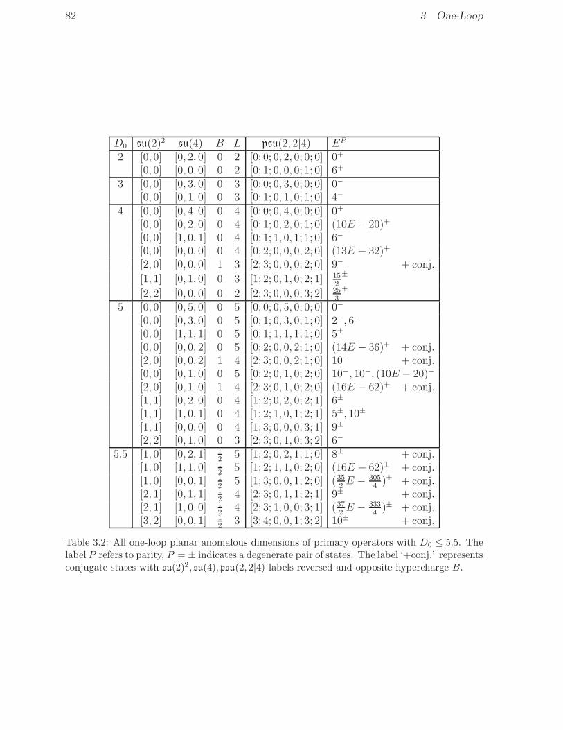
82 3 One-Loop
D0 su(2)2 su(4) B L psu(2, 2|4) EP
2 [0, 0] [0, 2, 0] 0 2 [0; 0; 0, 2, 0; 0; 0] 0+
[0, 0] [0, 0, 0] 0 2 [0; 1; 0, 0, 0; 1; 0] 6+
3 [0, 0] [0, 3, 0] 0 3 [0; 0; 0, 3, 0; 0; 0] 0−
[0, 0] [0, 1, 0] 0 3 [0; 1; 0, 1, 0; 1; 0] 4−
4 [0, 0] [0, 4, 0] 0 4 [0; 0; 0, 4, 0; 0; 0] 0+
[0, 0] [0, 2, 0] 0 4 [0; 1; 0, 2, 0; 1; 0] (10E − 20)+
[0, 0] [1, 0, 1] 0 4 [0; 1; 1, 0, 1; 1; 0] 6−
[0, 0] [0, 0, 0] 0 4 [0; 2; 0, 0, 0; 2; 0] (13E − 32)+
[2, 0] [0, 0, 0] 1 3 [2; 3; 0, 0, 0; 2; 0] 9− + conj.
[1, 1] [0, 1, 0] 0 3 [1; 2; 0, 1, 0; 2; 1] 152
±
[2, 2] [0, 0, 0] 0 2 [2; 3; 0, 0, 0; 3; 2] 253
+
5 [0, 0] [0, 5, 0] 0 5 [0; 0; 0, 5, 0; 0; 0] 0−
[0, 0] [0, 3, 0] 0 5 [0; 1; 0, 3, 0; 1; 0] 2−, 6−
[0, 0] [1, 1, 1] 0 5 [0; 1; 1, 1, 1; 1; 0] 5±
[0, 0] [0, 0, 2] 0 5 [0; 2; 0, 0, 2; 1; 0] (14E − 36)+ + conj.[2, 0] [0, 0, 2] 1 4 [2; 3; 0, 0, 2; 1; 0] 10− + conj.[0, 0] [0, 1, 0] 0 5 [0; 2; 0, 1, 0; 2; 0] 10−, 10−, (10E − 20)−
[2, 0] [0, 1, 0] 1 4 [2; 3; 0, 1, 0; 2; 0] (16E − 62)+ + conj.[1, 1] [0, 2, 0] 0 4 [1; 2; 0, 2, 0; 2; 1] 6±
[1, 1] [1, 0, 1] 0 4 [1; 2; 1, 0, 1; 2; 1] 5±, 10±
[1, 1] [0, 0, 0] 0 4 [1; 3; 0, 0, 0; 3; 1] 9±
[2, 2] [0, 1, 0] 0 3 [2; 3; 0, 1, 0; 3; 2] 6−
5.5 [1, 0] [0, 2, 1] 12
5 [1; 2; 0, 2, 1; 1; 0] 8± + conj.[1, 0] [1, 1, 0] 1
25 [1; 2; 1, 1, 0; 2; 0] (16E − 62)± + conj.
[1, 0] [0, 0, 1] 12
5 [1; 3; 0, 0, 1; 2; 0] (352E − 305
4)± + conj.
[2, 1] [0, 1, 1] 12
4 [2; 3; 0, 1, 1; 2; 1] 9± + conj.[2, 1] [1, 0, 0] 1
24 [2; 3; 1, 0, 0; 3; 1] (37
2E − 333
4)± + conj.
[3, 2] [0, 0, 1] 12
3 [3; 4; 0, 0, 1; 3; 2] 10± + conj.
Table 3.2: All one-loop planar anomalous dimensions of primary operators with D0 ≤ 5.5. Thelabel P refers to parity, P = ± indicates a degenerate pair of states. The label ‘+conj.’ representsconjugate states with su(2)2, su(4), psu(2, 2|4) labels reversed and opposite hypercharge B.

3.5 Planar Spectrum 83
fractional numbers but solutions to some algebraic equations. We refrain from solvingthese numerically, but instead give the equations. In the table such states are representedby polynomials X(E) of degree k − 1. The true energies E are obtained as solutions tothe equation
Ek = X(E). (3.72)
For example, the quadratic polynomial for the state with weight (4; 0, 0; 0, 2, 0; 0, 4) isX(E) = 10E − 20. It translates to the energy (see also [45])
E2 = 10E − 20, E = 5±√
5. (3.73)
The table was computed as follows: A C++ programme was used to determine allhighest weight states up to and including classical dimension 5.5 as well as their descen-dants. In analogy to the sieve of Eratostene the algorithm [105] subsequently removesdescendants from the set of all states. What remains, are the primary states. Pleaserefer to [106] for details of the implementation of the sieve algorithm. For each multipletwe pick one state and compute the total excitation numbers using Tab. D.2. Here it iscrucial to choose a descendant for which the mixing problem is minimised. This reducesthe size of the energy matrix to be computed and diagonalised. For these purposes, agood descendant usually has as few different types of oscillators as possible.
In a Mathematica programme all states with a given set of oscillator excitations werecollected: We spread the oscillators on the sites of the spin chain in all possible ways tak-ing the central charge constraint at each site into account. Identical states with respectto cyclicity of the trace are dropped. In a second step, the harmonic action, c.f. App. F,was applied to all the states to determine the matrix of anomalous dimensions. For allthe descendants which were removed in the sieve algorithm, we remove the correspond-ing energy eigenvalues. The remaining eigenvalues are the one-loop planar anomalousdimensions of highest weight states.
To go to higher canonical dimensions involves obtaining and diagonalising bigger andbigger matrices. One can reduce the complexity by going to certain subsectors. Thesmallest subsector is the su(2) subsector, see Sec. 2.4. There are only two fields, Z, φ,which we might indicate in a planar notation as
|0〉 = Z, |1〉 = φ. (3.74)
The Hamiltonian density acts on two adjacent fields, within this sector it is (2.110)
H′′′12 |k1, k2〉 = |k1, k2〉 − |k2, k1〉. (3.75)
Here there are far less states and it is much easier to compute the energy matrix. InTab. 3.4 we show a complete table of states and energies up to classical dimension D0 ≤ 9.We have omitted the vacuum states with K = 0; there is one for each length L andits energy vanishes. The states and their energies can be obtained conveniently usinga computer algebra system. In App. E we present a couple of Mathematica functionsto deal with the su(2) subsector. Similarly, we can obtain the spectrum for the bosonicsu(1, 1) subsector. The expression (3.70) can be used to calculate any one-loop anomalousdimension within this subsector. We display our results in Tab. 3.6.
There are two points to be observed in the spectra in Tab. 3.2,3.4,3.6. Firstly, we notethe appearance of pairs of states with degenerate energy and opposite parities P = ±
‘paired state’: E+ = E−. (3.76)

84 3 One-Loop
L K EP
4 2 6+
5 2 4−
6 2 (10E − 20)+
3 6−
7 2 2−, 6−
3 5±
L K EP
8 2 (14E2 − 56E + 56)+
3 4±, 6−
4 (20E2 − 116E + 200)+
9 2 (8E − 8)−, 4−
3 (17E2 − 90E + 147)±
4 5±, (12E − 24)−
Table 3.4: The lowest-lying states within the su(2) subsector [38]. The weights of the corre-sponding primaries are (L− 2; 0, 0;K − 2, L− 2K,K − 2; 0, L − 2).
D0 L K EP
4 2 2 6+
5 3 2 4−
6 4 2 (10E − 20)+
3 3 152
±
2 4 253
+
7 5 2 2−, 6−
4 3 6±
3 4 6−
D0 L K EP
8 6 2 (14E2 − 56E + 56)+
5 3 (252E − 147
4)±
4 4 233
±, (73
3E2 − 553
3E + 1274
3)+
3 5 354
±
2 6 495
+
9 7 2 (8E − 8)−, 4−
6 3 (19E2 − 4594E + 216)±
5 4 (13E − 32)−, (976E − 2291
36)±
4 5 (352E − 665
9)±
3 6 223
−, 227
20
±
Table 3.6: The first few states within the bosonic su(1, 1) subsector [50]. The weights of thecorresponding primaries are (L + K − 2;K − 2,K − 2; 0, L − 2, 0; 0, L).
This will be an important issue for integrability discussed in Ch. 4. Secondly, we findsome overlapping primaries in Tab. 3.4,3.6, clearly their energies do agree. What is more,we find that a couple of energies repeatedly occur. These are for example, 6, 10, 5, 9,but also 10E − 20 and 13E − 32. As these states are primaries transforming in differentrepresentations, they cannot be related by psu(2, 2|4). Of course, these degeneracies couldmerely be a coincidence of small numbers. Nevertheless the reappearance of e.g. 13E−32is somewhat striking. This could hint at yet another symmetry enhancement of theplanar one-loop Hamiltonian. It might also turn out to be a consequence of integrability.Furthermore, one might speculate that it is some remnant of the broken higher spinsymmetry of the free theory, see e.g. [107] and references in [105].
3.5.2 Two Partons
A straightforward exercise is to determine the spectrum of states of length L = 2.These so-called twist-two states can conveniently be written as
Oj,AB = (Pj)CDABTrWCWD. (3.77)

3.5 Planar Spectrum 85
Note that j must be even due to cyclicity of the trace. Using (3.60) we find6
E = 4h(j), δD =g2
YMN
2π2h(j) +O(g3) (3.78)
in agreement with the results of [43, 44]. Twist-two states have positive parity.
3.5.3 Three Partons
For states of length L = 3 the following multiplets are found within a trace [103]
TrVF × VF × VF =∞∑
m=−∞
∞∑
n=0
(V−
2m,2n + V+2m+1,2n + cnV±
m,n+3
), (3.79)
where c0,1,2,3,4,5 = (1, 0, 1, 1, 1, 1) and cn+6 = cn + 1. The modules Vm,n have highestweights
w0,0 = (3; 0, 0; 0, 3, 0; 0, 3),
w0,n = (n+ 1;n− 2, n− 2; 0, 1, 0; 0, 3),
w1,0 = (3; 0, 0; 0, 0, 0; 0, 3),
w1,n = (n+ 5/2;n, n− 1; 0, 0, 1; 1/2, 3),
wm,n = (n+ 2m;n+ 2m− 2, n+m− 2; 0, 0, 0; 1, 3) (3.80)
and the conjugate w−m,n has reversed su(2)2, su(4) labels and opposite hypercharge. Themultiplets V0,n have components in the subsector (2, 2), see (3.4), the multiplets V1,n
have components in the fermionic subsector (3, 1), see (3.2), and all the other Vm,n arerepresented in the sector (4, 0).
By inspecting the spectrum of lowest-lying states and their energies, we find thatalmost all of them form pairs with degenerate energies. We list the pairs in Tab. 3.8.7
Concerning the unpaired states, there is one for each even n, it has parity (−1)m+1. Forthe unpaired states one can observe a pattern in the table of energies, Tab. 3.10. We findthat all energies agree with the formula
E = 2h(12m− 1
2) + 2h(m+ 1
2n) + 2h(1
2m+ 1
2n)− 2h(−1
2). (3.81)
In particular, for m = 1 the energies are
E = 2h(1 + 12n) + 2h(1
2+ 1
2n)− 2h(−1
2) = 4h(n+ 2), (3.82)
which agrees precisely with the energy (3.78) of the short twist-two multiplet V2n+2.Superconformal invariance requires this degeneracy so that the short multiplets can jointo form a long multiplet. The cases m = 0 and n = 0 also seem interesting, we findE = 4h(1
2n) and E = 6h(m).
6Note that H = H12 +H21 = 2H12 = 4h(J12).7The energies are all rational numbers because there is always just a single pair up to n ≤ 8 (3.79).
Starting from n = 9 there is more than one pair and the energies become irrational.

86 3 One-Loop
n\m 0 1 2 3 4 5 6
3 152
10 474
13110
715
105970
4461280
5 354
13312
76160
48735
12533840
397492520
13873840
6 22720
76160
96770
2069140
393492520
2747168
3929231
7 58160
17915
3763280
183831260
391332520
7543462
943735544
8 5087420
1403105
181871260
386772520
497113080
2593154
62922736036
Table 3.8: First few paired anomalous dimensions for Vm,n [103].
n\m 0 1 2 3 4 5 6
0 0 6 9 11 252
13710
14710
2 4 253
323
12310
40730
3067210
54235
4 6 495
716
92970
725
9661630
2259140
6 223
76170
19115
8851630
52835
22104713860
210311260
8 253
7381630
20215
1018616930
6581420
32989920020
216431260
10 13715
860216930
49335
2748871180180
203831260
20354512012
1220296930
Table 3.10: First few unpaired anomalous dimensions for Vm,n [103]. The parity is P = (−1)m+1.
3.5.4 Two Excitations
Instead of considering a fixed number of fields, one can also consider the L-particlevacuum state |Z, L〉 and add a small number of excitations, see Sec. 2.3.6. A state withoutexcitations is just the half-BPS vacuum and a state with one excitation is related to thevacuum by one of the lowering operators. The first interesting case is two excitations [14].Assume we consider four oscillator excitations of type a†
2, a†2,b
†2,b
†2. This corresponds to
a state of the bosonic su(1, 1) sector with a total of two derivatives D acting on L fieldsZ. A useful basis of states is thus
EL1 = TrDDZ ZL−1, ELp = TrDZ Zp−2DZ ZL−p. (3.83)
Note that we should identify ELp and ELL+2−p due to cyclicity of the trace and consider amatrix with half the number of rows and columns. Equivalently, we may choose to restrictto vectors which are symmetric under p ↔ L+ 2 − p. Using the Hamiltonian (3.70), wefind the matrix of anomalous dimensions in this basis
H =
+2 −1 −1−2 +4 −2
−2. . .
. . .. . .
. . . −2−2 +4 −2
−2 −2 +4
. (3.84)
The bulk of the matrix has precisely the form of a second lattice derivative. Theappropriate ansatz to diagonalise it, is a vector with elements cos(ap+ b). The boundarycontributions together with the symmetry determine the constants a and b. The matrix

3.5 Planar Spectrum 87
(3.84) has the following exact eigenvectors
OLn =1
L
L∑
p=1
cos
(πn(2p− 1)
L+ 1
)ELp . (3.85)
Note that OLn = OL−n = −OLL+1−n. Thus the set of independent modes is given by themode numbers 0 ≤ n < (L + 1)/2. The corresponding exact planar one-loop anomalousdimension is [27]
ELn = 8 sin2 πn
L+ 1, δD =
g2YMN
π2sin2 πn
L+ 1+O(g3). (3.86)
This is just one component of a multiplet of the residual symmetry psu(2|2)×psu(2|2)within the sector. The oscillators A† = (a†, c†) (c.f. Sec. 2.3.6) transform in the fun-damental representation [0; 0; 1] of one of the psu(2|2)’s. For two excitations we shouldconsider the tensor product of two fundamental modules which is [0; 0; 1] × [0; 0; 1] =[0; 0; 2]+ + [0; 1; 0]−. These two correspond to the symmetric and antisymmetric combi-nation of two indices A,B. The same applies to the oscillators A† = (b†,d†). In total wefind four multiplets corresponding to the combined symmetrisations ++,+−,−+,−−:
OLn,{AB]{CD]
=L∑
p=1
cos
(πn(2p− 1)
L+ 1
)TrA†
1,{AA†p,B] A
†1,{CA†
p,D]|Z, L〉,
OL+1
n,{AB][CD} =
L+1∑
p=2
sin
(πn(2p− 2)
L+ 1
)TrA†
1,{AA†p,B] A
†1,[C
A†p,D} |Z, L+ 1〉,
OL+1
n,[AB}[CD]=
L+1∑
p=2
sin
(πn(2p− 2)
L+ 1
)TrA†
1,[AA†p,B} A
†1,{CA†
p,D]|Z, L+ 1〉,
OL+2
n,[AB}[CD} =
L+2∑
p=2
cos
(πn(2p− 3)
L+ 1
)TrA†
1,[AA†p,B} A†
1,[CA†p,D} |Z, L+ 2〉. (3.87)
All of these have the same energy ELn . This is related to the fact that all short multiplets
join to form a long multiplet in the interacting theory [27] (unless n = 0). For psu(2|2)the interacting multiplet [0; 1 + 1
2δD; 0] is at the unitarity bound r1 ≈ s1 + 1. When
δD approaches zero, the interacting multiplet splits up into a short and a BPS multiplet[0; 1 + 1
2δD; 0] → [0; 1; 0] + [0; 0; 2]. In total, the highest weight of the long multiplet is
therefore[0; 1 + 1
2δD; 0]× [0; 1 + 1
2δD; 0]. (3.88)
In psu(2, 2|4) the classical highest weight for states n 6= 0 is (L; 0, 0; 0, L− 2, 0; 0, 0) =[0; 1; 0, L− 2, 0; 1; 0]. The protected states for n = 0 are part of the half-BPS multiplet(L; 0, 0; 0, L, 0; 0, 0). The states have parity (−1)L.
3.5.5 Three Excitations
Let us investigate the states with three excitations. We find that such states almostalways form pairs with degenerate planar energies. The only exceptions from this rule are

88 3 One-Loop
states with weight
(2m+ 4; 0, 0; 1, 2m, 1; 0, 2m+ 4) = [0; 1; 1, 2m, 1; 1; 0], m ≥ 0. (3.89)
They have a descendant in the su(2) subsector which is given by
O =
2m+2∑
k=1
(−1)k TrφφZkφZ2m+3−k, E = 6, P = −1. (3.90)
Interestingly, two of the excitations are always adjacent in this leading order approxima-tion. Further states of this kind with more excitations can be found.
3.6 Plane Wave Physics
In this section we would like to demonstrate the use of the dilatation operator tofind non-planar corrections, i.e. corrections in 1/N , to the scaling dimensions. Here thedilatation operator brings about a major simplification [35] as opposed to the computationof correlation functions [18,19,108,21,22,36] because it allows to derive scaling dimensionsindependently of two-point normalisation constants. In particular we will derive thegenus-one correction to the scaling dimension of two-excitation BMN operators in theBMN limit.
3.6.1 The BMN Limit
Berenstein, Maldacena and Nastase (BMN) [14] suggested to investigate operators ofa large dimension D0 and a nearly equally large charge J of su(4)
J = p− 12q1 − 1
2q2. (3.91)
Then the relevant states constitute long strings of Z-fields with D0 − J excitations orimpurities scattered in8
TrZ . . .Z φZ . . .Z DZ Z . . .Z ψZ . . .Z, (3.92)
which became known as BMN operators. As particular examples, BMN investigatedoperators with zero, one and two excitations of scalar type. The operators with less thantwo excitations belong to half-BPS multiplets and are thus protected. Starting with twoexcitations there are states whose scaling dimension changes in the quantum theory. Forlarge J one finds that the smallest one-loop planar anomalous dimensions scale as 1/J2,
E = O(1/J2). (3.93)
as confirmed by the exact values in the case of two excitations (3.86). BMN proposed toabsorb the dependence on J into an effective coupling constant λ′
λ′ :=λ
J2=g2
YMN
J2, (3.94)
8The excitation subsectors in Sec. 2.3.6 were constructed to describe states of this kind.

3.6 Plane Wave Physics 89
for our purposes it seems convenient to use the combination g
g :=g
J, λ′ = 8π2g2. (3.95)
BMN conjectured that this would lead to finite planar eigenvalues for the BMN energyoperator D− J (as a function of g) in the large J limit, even beyond one-loop.
Moreover, it was found [18, 19] that also the genus counting parameter 1/N can berenormalised in such a way as to obtain finite results for non-planar correlators
gs = g2 :=J2
N. (3.96)
The non-planar BMN limit can be defined as the double-scaling limit
‘BMN limit ’: J,N, g, λ→∞ with g, gs fixed. (3.97)
The physical significance of the above lies in the BMN correspondence, which is a limitof the celebrated AdS/CFT correspondence. The statement of the correspondence is thatBMN operators are dual to states of string theory on the plane-wave background. Thescaling dimensions of BMN operators minus their charge J should match the light-coneenergies of the corresponding string states. In an operatorial form, the correspondencecan be written as
‘BMN Correspondence’: HLC = D− J +O(1/J). (3.98)
The planar limit corresponds to a non-interacting string theory and it is fairly easy toderive the light-cone energy eigenvalues [14]
ELC =
M∑
k=1
√1 + λ′ n2
k =
M∑
k=1
√1 + 2g2(2πnk)2 . (3.99)
The numbers nk are the mode numbers (positive, negative or zero) of M string oscillatorexcitations and are subject to the level matching constraint
∑Mk=1 nk = 0. There are some
indications that this all-loop prediction for gauge theory might indeed be true [25, 109].There exists an exceedingly large literature on the BMN correspondence, see [17] for
reviews.
3.6.2 Basis of States
Starting from here, we will only consider operators with two excitations. As shown inSec. 3.5.4, it makes perfect sense to consider these operators also for arbitrary finite valuesof J . All two-excitation states form a single multiplet of superconformal symmetry, so weare free to choose a particular descendant to be used in our investigation. In particularthere is one descendant in the su(2) sector that can be written in terms of J fields Z andtwo excitations of type φ. Generic multi-trace operators with two excitations can haveboth excitations in one trace
EJ0;J1,...,JKp = TrφZpφZJ0−p
K∏
k=1
TrZJk , (3.100)

90 3 One-Loop
or the two excitations separated in different traces
QJ0,J1;J2,...,JK = TrφZJ0 TrφZJ1
K∏
k=2
TrZJk , (3.101)
with∑K
k=0 Jk = J . Both series of operators are symmetric under the interchange of sizesJk of traces TrZJk , E is symmetric under p→ J0− p and Q is symmetric under J0 ↔ J1.
3.6.3 The Action of the Dilatation Generator
The non-planar dilatation generator (2.113)
H = D2 = −N−1:Tr [Z, φ][Z, φ]: (3.102)
can be seen to act as
H(Ep Q
)=(Ep Q
)( ∗ ∗0 0
), (3.103)
i.e. operators of type Q are never produced. This follows from the fact that all producedobjects will contain a commutator [Z, φ] in some trace and this trace will vanish unlessit contains another φ. It immediately follows that for every Q there is one protectedquarter-BPS operator. Its leading part is given by Q itself, plus a 1/N correction fromthe operators Ep [34, 110, 21, 22].9 On the other hand, the operators Ep are in general notprotected and we will investigate their spectrum of anomalous dimensions in what follows.From the form of the dilatation matrix we infer that operators of type Ep do not receivecorrections from operators of type Q; the latter therefore completely decouple as far asthe consideration of the Ep’s is concerned.
It is easy to write down the exact expression for HEp. Let us define
H = H0 +N−1H+ +N−1H−, (3.104)
where H0 is trace conserving and H+ and H− respectively increases and decreases thenumber of traces by one. These three different contributions arise from three differentcontractions of the variations in the dilatation generator with the fields in the states,see Fig. 3.6. Contractions to adjacent fields within a trace lead to planar contributions.Contractions to non-adjacent fields will split up the trace. Contractions to different traceswill join them. We find
H0 EJ0;J1,...,JKp = −2
(δp 6=J0
EJ0;J1,...,JK
p+1 − (δp 6=J0+ δp 6=0)EJ0;J1,...,JK
p + δp 6=0EJ0;J1,...,JK
p−1
),
H+ EJ0;J1,...,JKp =
p−1∑
JK+1=1
2(EJ0−JK+1;J1,...,JK+1
p−JK+1− EJ0−JK+1;J1,...,JK+1
p−1−JK+1
)
−J0−p−1∑
JK+1=1
2(EJ0−JK+1;J1,...,JK+1
p+1 − EJ0−JK+1;J1,...,JK+1
p
),
9We note that all quarter-BPS states in [34, 110] are annihilated by the operator [Z, φ] which is partof D2. It is also part of a superboost which relates would-be quarter-BPS states with their partners in along multiplet. For true quarter-BPS states, this must not happen and [Z, φ] annihilates them.

3.6 Plane Wave Physics 91
H
O O
H H
O1 O2
↓ ↓ ↓
O′ O′1 O′
2 O′
Planar H0 Splitting H+ Joining H−
Figure 3.6: Topological structures of the action of the one-loop dilatation operator.
H− EJ0;J1,...,JKp =
K∑
k=1
2Jk(EJ0+Jk;J1,...,×Jk,...,JK
Jk+p − EJ0+Jk;J1,...,×Jk,...,JK
Jk+p−1
)
−K∑
k=1
2Jk(EJ0+Jk;J1,...,×Jk,...,JK
p+1 − EJ0+Jk;J1,...,×Jk,...,JKp
). (3.105)
In view of the AdS/CFT and BMN correspondence this is very suggestive. The one-loopdilatation operator can either not change the structure of traces, split one trace into two,or join two into one. This is in qualitative agreement with string field theory when tracesare interpreted as strings. Also the parameter 1/N appears in the right places to beinterpreted as the string coupling constant.
3.6.4 The BMN Limit of Two Excitation Operators
With J being very large we can view p = p/J and Jk = Jk/J as continuum variablesand replace the discrete set of states in equation (3.100) by a set of continuum states
EJ0;J1,...,JKp → |p; J1, . . . , JK〉 = |J0 − p; J1, . . . , JK〉, (3.106)
where
p ∈ [0, J0], J0, Jk ∈ [0, 1] and J0 = 1− (J1 + . . .+ JK). (3.107)
It is understood that |p; J1, . . . , JK〉 = |p; Jπ(1), . . . , Jπ(K)〉 with π an arbitrary permutationof K elements.
Absorbing the J-dependence into the definition of the Hamiltonian
H = J2H and H = H0 + gsH+ + gsH−, (3.108)

92 3 One-Loop
we impose the BMN limit (3.97) and get a continuum version of (3.105)
H0 |p; J1, . . . , JK〉 = −2∂2p |p; J1, . . . , JK〉, (3.109)
H+ |p; J1, . . . , JK〉 =
p∫
0
dJK+1 2∂p|p− JK+1; J1, . . . , JK+1〉
−J0−p∫
0
dJK+1 2∂p|J ; J1, . . . , JK+1〉,
H−|p; J1, . . . , JK〉 =K∑
k=1
2Jk ∂p|p+ Jk; J1, . . . , ×Jk, . . . , JK〉
−K∑
k=1
2Jk ∂p |p; J1, . . . , ×Jk, . . . , JK〉.
3.6.5 The Mode Decomposition
The (K + 1)-trace eigenstates at gs = 0 are
|n; J1, . . . , JK〉 =1
J0
∫ J0
0
dp cos(
2πnJ0
p)|p; J1, . . . , JK〉, n = 0, 1, 2, . . . . (3.110)
This is of course in accordance with the nature of the exact eigenstates at finite J ,c.f. Sec. 3.5.4. The inverse transformation of (3.110) reads
|p; J1, . . . , JK〉 = |0; J1, . . . , JK〉+ 2∞∑
n=1
cos(
2πnJ0
p)|n; J1, . . . , JK〉. (3.111)
In the basis (3.110), the action of the operator H reads
H0 |n; J1, . . . , JK〉 = 2(
2πnJ0
)2 |n; J1, . . . , JK〉, (3.112)
H+ |n; J1, . . . , JK〉 =16
J0
∫ J0
0
dJK+1
∞∑
n′=1
(2πn′
J0−JK+1
)2sin2
(πn JK+1
J0
)
(2πn′
J0−JK+1
)2 −(
2πnJ0
)2 |n′; J1, . . . , JK+1〉,
H−|n; J1, . . . , JK〉 = 16K∑
k=1
Jk
J0
∞∑
n′=1
(2πn′
J0+Jk
)2sin2
(πn′ Jk
J0+Jk
)
(2πn′
J0+Jk
)2 −(
2πnJ0
)2 |n′; J1, . . . , ×Jk, . . . , JK〉.
In interacting plane-waves string theory similar expressions have been derived [20,111,23,112]. The Hamiltonians of both theories should however not be compared directly, butonly modulo a similarity transformation. A proposal for the change of basis was givenin [24, 113] and applied in [47] to show the equivalence of the Hamiltonians in the one-loop approximation. Up to some assumptions [23] (which appear to be inconsistent [114])regarding excitation number non-preserving amplitudes in string theory, it proves theBMN correspondence (3.98) at first order in g2 (one-loop) and all orders in gs (all-genus)for single trace states with two excitations. A similar statement for three excitation stateswas investigated in [115], but a generalisation to arbitrarily many excitations of arbitrarytype has not been attempted yet.
3.6 Plane Wave Physics 93
3.6.6 The Genus-One Energy Shift
Now the scene is set for determining the spectrum of the full one-loop Hamiltonianorder by order in gs by standard quantum mechanical perturbation theory. The leadingnon-planar correction to the energy En,0 = 2(2πn)2 of a single trace state |n〉 is obtainedby second-order perturbation theory
En,2|n〉 = πn H−1
En,0 − H0
H+ |n〉, (3.113)
where πn projects to |n〉. We now insert (3.112) and get the genus-one (torus) correctionto the energy
En,2 =
∫ 1
0
dJ1
∞∑
n′=1
128 J1(2πn′
1−J1
)2(2πn)2 sin4(πnJ1)
(1− J1)(( 2πn′
1−J1
)2 − (2πn)2
)3 =1
6+
35
4(2πn)2. (3.114)
The total scaling dimension is thus
D = J + 2 + 2(2πn)2g2 +
(1
6+
35
4(2πn)2
)g2g2
s + . . .
= J + 2 + λ′ n2 + λ′g2s
(1
48π2+
35
128π4n2
)+ . . . . (3.115)
This genus-one result was first derived by computing gauge theory correlation functions[21, 22] and confirmed in string theory [23], see also [24]. Here it was assumed that onecan restrict to excitation number preserving amplitudes in string theory, however, thereare doubts that this assumption is consistent [114]. Subsequently, the formula (3.114) wasrederived by Janik by considering matrix elements of the dilatation generator [37]. Thislead to a great simplification of the calculation.

94
95
Chapter 4
Integrability
In Sec. 2.6 we have demonstrated how, in the planar limit, local operators can beinterpreted as quantum spin chains. In that picture, the planar dilatation operator isrepresented by the spin chain Hamiltonian. Minahan and Zarembo realised that the one-loop dilatation operator of N = 4 SYM for states composed from only scalar fields (theone-loop so(6) sector) is precisely the Hamiltonian of an integrable spin chain [48]. Thisparallels earlier discoveries of integrable spin chains in generic, non-supersymmetric gaugetheories at one-loop and in the large N limit when dealing with states composed mostlyfrom covariant derivatives [52–54] (see also the review [55]).
In this chapter we will show how these two lines of development can be combined intoa psu(2, 2|4) supersymmetric spin chain [58]. We will start by introducing the notionof integrable spin chains and later present the algebraic Bethe ansatz technique. Asan application, we shall derive the one-loop anomalous dimension of a state dual to amacroscopic spinning string in AdS5 × S5 and find a remarkable agreement [60, 66].
4.1 Integrable Spin Chains
A quantum integrable system is a quantum mechanical system with an infinite number1
of mutually commuting scalar charges Qr
[Qr,Qs] = [J,Qr] = 0. (4.1)
In other words, the naive symmetry algebra is enlarged by infinitely many abelian genera-tors constituting the algebra u(1)∞. The Hamiltonian H, a u(1) generator invariant underthe symmetry algebra, will turn out to be one of the charges, H = Q2, and is absorbedinto u(1)∞. The symmetry enhancement might thus be stated as
u(1) −→ u(1)∞. (4.2)
In this section we will discuss the integrable structures found at the one-loop level.
1The precise counting is somewhat unclear in a quantum system. In a classical system one needsexactly half the number of phase-space dimensions. Here, the spin chains can be arbitrarily long whichgives rise to an arbitrarily large number of conserved charges. This is what is meant by infinitely many.

96 4 Integrability
u1, A1
u1, B1
u2, A2
u2, B2
R A1A2
B1B2
(u1 − u2)
Figure 4.2: A scattering process of two particles is described by the R-matrix.
R
R
R
=
R
R
R
Figure 4.4: The Yang-Baxter equation.
4.1.1 The R-Matrix
A spin chain is composed from L modules transforming in some representation of asymmetry algebra. We will assume the symmetry algebra to be of unitary type, su(M).To understand the integrable model, it makes sense to consider the individual spins as‘particles’. A particle XA(u) is thus defined as an element of a module of the symmetrygroup together with a spectral parameter u. The central object of the integrable model isthe R-matrix, it describes the ‘scattering’ of particles. The R-matrix rotates two modulesdepending on their representations and difference of spectral parameters, c.f. Fig. 4.2
X ′2,B2
(u2)X′1,B1
(u1) = RA1A2
B1B2(u1 − u2)X1,A1
(u1) X2,A2(u2). (4.3)
The scattering is elastic in the sense that neither the representation nor the spectralparameters are changed; the only effect is a generalised phase shift described by the R-matrix. In an integrable system, the order in which particles scatter does not matter. Forthe scattering of three particles this fact is described by the Yang-Baxter equation
RA1A2
B1B2(u1 − u2)RB1A3
C1B3
(u1 − u3)RB2B3
C2C3
(u2 − u3)
= RA2A3
B2B3
(u2 − u3)RA1B3
B1C3
(u1 − u3)RB1B2
C1C2(u1 − u2) (4.4)
or R12R13R23 = R23R13R12 for short. The Yang-Baxter equation is most intuitivelyrepresented in a diagrammatic fashion, see Fig. 4.4; it implies that the particle lines canbe moved around freely, even past other interactions. From this it follows that, also for alarger number of particles, the order of scatterings does not matter.
In addition to the Yang-Baxter equation, there is the relation, see Fig. 4.6
RA1A2
B1B2(u1 − u2)RB2B1
C2C1(u2 − u1) = δA1
C1δA2
C2, (4.5)
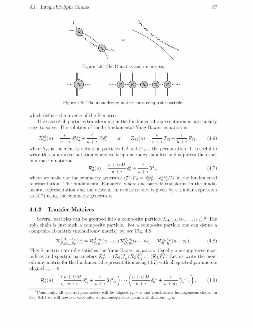
4.1 Integrable Spin Chains 97
R
R
=
Figure 4.6: The R-matrix and its inverse.
R = R R R R R
Figure 4.8: The monodromy matrix for a composite particle.
which defines the inverse of the R-matrix.The case of all particles transforming in the fundamental representation is particularly
easy to solve. The solution of the bi-fundamental Yang-Baxter equation is
Rabcd(u) =
u
u+ iδac δ
bd +
i
u+ iδadδ
bc or R12(u) =
u
u+ iI12 +
i
u+ iP12, (4.6)
where I12 is the identity acting on particles 1, 2 and P12 is the permutation. It is useful towrite this in a mixed notation where we keep one index manifest and suppress the otherin a matrix notation
Rab (u) =
u+ i/M
u+ iδab +
i
u+ iJab, (4.7)
where we make use the symmetry generator (Jab)cd = δadδ
cb − δab δcd/M in the fundamental
representation. The fundamental R-matrix, where one particle transforms in the funda-mental representation and the other in an arbitrary one, is given by a similar expressionas (4.7) using the symmetry generators.
4.1.2 Transfer Matrices
Several particles can be grouped into a composite particle XA1...AL(v1, . . . , vL).
2 Thespin chain is just such a composite particle. For a composite particle one can define acomposite R-matrix (monodromy matrix) by, see Fig. 4.8
RA,A1...AL
B,B1...BL(u) = RA A1
C2B1(u− v1)RC2A2
C3B2(u− v2) . . .RCLAL
B BL(u− vL). (4.8)
This R-matrix naturally satisfies the Yang-Baxter equation. Usually one suppresses mostindices and spectral parameters RA
B = (R1)AC2
(R2)C2
C3. . . (RL)
CL
B . Let us write the mon-odromy matrix for the fundamental representation using (4.7) with all spectral parametersaligned vp = 0
Rab (u) =
(u+ i/M
u+ iδac2 +
i
u+ iJ1
ac2
)· · ·(u+ i/M
u+ iδcLb +
i
u+ uLJL
cLb
). (4.9)
2Commonly, all spectral parameters will be aligned vp = v and constitute a homogeneous chain. InSec. 6.4.1 we will however encounter an inhomogeneous chain with different vp’s.

98 4 Integrability
This expression reveals an interesting interpretation of the monodromy matrix for a spinchain: The generator of rotations, J, may be considered as the component of some gaugefield in the direction of the spin chain. Then, the monodromy matrix has a great similarityto a Wilson line along the spin chain. In that picture, an elementary R-matrix is just themonodromy of the gauge field across one spin chain site. Moreover, there is not only asingle gauge field, but a family of gauge fields, parameterised by the spectral parameteru. When viewed in this way, the integrable structure is very similar to the one found instring theory on AdS5 × S5, see [82, 83, 86]. This similarity allowed the authors of [116]to promote the Yangian structure from string theory to gauge theory.
For a cyclic spin chain it is natural to close the Wilson line to a loop and take thetrace. One obtains the transfer matrix
T (u) = RAA(u) = (R1)
C1
C2(R2)
C2
C3. . . (RL)
CL
C1. (4.10)
The transfer matrix can be taken for any representation circulating around the Wilsonloop and for any spectral parameter. In this work, however, we shall restrict to theequal representations of the spins and the Wilson loop. The interesting aspect of transfermatrices is that all of them commute
[T (u), T (v)] = 0. (4.11)
This statement can be shown easily by inserting a R-matrix and its inverse into thetraces, see Fig. 4.6. Using the Yang-Baxter equation, the R-matrix is commuted aroundthe traces interchanging the order of monodromy matrices
T (u) T (v) = RAA(u) RA
A(v) = RAA
BB(v − u)RBB
CC(u− v) RC
A(u) RC
A(v)
= RAABB
(v − u) RBC(v) RB
C(u)RCC
AA(u− v)
= RBB(v) RB
B(u) = T (v) T (u). (4.12)
Afterwards the R-matrix and its inverse cancel out and the transfer matrices are inter-changed.
4.1.3 The Local Charges
There are many uses for monodromy and transfer matrices. A particular one is theYangian, an associative Hopf algebra which enlarges the symmetry algebra, see e.g. [117].The Yangian is an important object for integrable systems. The elements of the Yangianare given by the monodromy matrix in the fundamental representation (4.8). Commonly,the Yangian is expanded around u =∞. In the leading two orders one finds the identityand the generators of the symmetry algebra, J, acting on the full spin chain. At the nextorder, the first non-trivial elements of the Yangian appear. They are bi-local along thespin-chain and can be used to generate all higher elements. In N = 4 SYM we deal withcyclic spin chains and the open Wilson line of the Yangian breaks cyclic symmetry. Atthe moment it is not clear how to make direct use of the Yangian for the study of scalingdimension and we will not consider it further. See [116] for a treatment of the Yangian inN = 4 SYM.

4.1 Integrable Spin Chains 99
Here we would like to investigate the transfer matrices. These are closed Wilson loopsand they preserve cyclic symmetry. The transfer matrix can be used as a generatingfunction for the charges U ,Qn when expanded in the spectral parameter
T (u) = U exp
∞∑
r=2
iur−1Qr. (4.13)
All of these charges commute with each other due to commuting of the transfer matricesat different values of the spectral parameters (4.11).
For spin chains with equal spin representations at each site, it is useful to pick thesame representation to circle around the Wilson loop as well. We will furthermore assumethat all R-matrices for the construction of the transfer matrix are the same and have aspecific value at u = 0
RA1A2
B1B2(0) = δA1
B2δA2
B1, (4.14)
i.e. they permute the modules.3 Let us now expand the transfer matrix in u. At u = 0we find the cyclic shift operator
UA1...AL
B1...BL= T A1...AL
B1...BL(0) = δA1
B2δA2
B3. . . δ
AL−1
BLδAL
B1. (4.15)
Expanding to first order in u we find that we have to insert a derivative R′ = ∂R/∂u ofthe R-matrix into the shift operator and sum over all insertion points,
T A1...AL
B1...BL(u) = UA1...AL
B1...BL+ u
L∑
p=1
δA1
B2. . .R′ ApAp+1
Bp+2Bp+1(0) . . . δAL
B1+O(u2). (4.16)
Let us define the charge density
Q2,A1A2
B1B2= −iR′ A1A2
B2B1(0) or Q2,12 = −iP12R′
12(0), (4.17)
where the second form is short for the first. The permutation P12 interchanges the spinsat two sites. According to the definition (4.13) we should absorb the cyclic shift in (4.16)into U and the second charge Q2 is simply
Q2,A1...AL
B1...BL=
L∑
p=1
δA1
B1. . .Q2,
ApAp+1
BpBp+1. . . δAL
BLor Q2 =
L∑
p=1
Q2,p,p+1. (4.18)
It is very suggestive to interpret this charge as the Hamiltonian, it has a nearest-neighbourtype interaction as desired for a spin chain
H = Q2 =
L∑
p=1
Hp,p+1, H12 = Q2,12 = −iP12R′12(0). (4.19)
Expanding T (u) to quadratic order in u we find many terms. There are some disconnectedterms which should be absorbed into −1
2u2UQ2
2 from the expansion of the exponential in(4.13). To complete the square Q2
2 we need the identity R′′12(0) = R′
12(0)P12R′12(0) due to

100 4 Integrability
Q3 =i
2 H
H− i
2
H
H
Figure 4.10: The third charge density is composed from two copies of the Hamiltonian density.
the Yang-Baxter equation. The remaining terms give rise to the third charge, see Fig. 4.10
Q3 =
L∑
p=1
Q3,p,p+1,p+2, Q3,123 = i2(H12H23 −H23H12). (4.20)
One can go on constructing the higher charges Qr in this way and finds that they can allbe written in terms of the Hamiltonian density H12.
4
4.1.4 Parity and Pairs
Above we have constructed two charges of the spin chain, H = Q2 and Q3. From(4.1,4.11) we know that they commute
[H,Q3] = 0, (4.21)
even though this statement is labourious to verify explicitly. Let us find out what happenswhen we invert the order of spins within the spin chain. This is equivalent to the parityoperation p defined in Sec. 1.3,2.6.4. up to a factor of (−1)L. The Hamiltonian densitywill be assumed to have positive parity
pH p−1 = H, [p,H] = 0. (4.22)
From this it immediately follows that the third charge has negative parity (it has negativemirror symmetry with respect to the vertical axis, see Fig. 4.10)
pQ3 p−1 = −Q3, {p,Q3} = 0. (4.23)
Similarly one finds for the higher charges
pQr p−1 = (−1)rQr. (4.24)
A consequence of (4.22,4.23,4.24) is that the spectrum of H will display a degeneracyof states |±〉 with opposite parities [118]
‘paired state’:{|+〉, |−〉
}with E+ = E−. (4.25)
3One might have to redefine the R-matrix slightly exploiting the symmetries of the Yang-Baxterequation (4.4): Firstly, we can rescale the R-matrix by a function of the spectral parameter. Secondly,we can shift and rescale the spectral parameters by a constant. The bi-fundamental R-matrix in (4.7) isalready in this from.
4A more efficient way is to use the boost operator B =∑L
p=1 ipHp,p+1. It generates the higher chargesrecursively via [B,Qr] = rQr+1. This can be deduced by assigning different spectral parameters to theindividual spins, up = u+pǫ. Note however, that the boost leaves some undesired boundary terms whichare, in particular, incompatible with the cyclic nature of the spin chain. These should be dropped.

4.2 One-Loop Integrability 101
This is a very non-trivial statement because H conserves parity and thus cannot relatestates with opposite parities in any way. Assume we find a state of positive parity |+〉and energy E+. Then the state |−〉 = Q3|+〉 has negative parity and energy E+
H |−〉 = HQ3 |+〉 = Q3H |+〉 = E+Q3 |+〉 = E+ |−〉. (4.26)
Of course, we cannot exclude that Q3 annihilates |+〉 and |−〉 = 0. In this case the stateof definite parity P = + or P = − is unpaired
‘unpaired state’: |P 〉 with Q3|P 〉 = 0. (4.27)
Such states exist when, for example, the numbers of positive and negative parity statesdo not agree.
We have seen that the third charge of the integrable spin chain has important conse-quences. It is thus natural to investigate the higher charges Qr. In contrast to Q3 we findthat Q4 does not pair up operators, it simply assigns a number (charge) to each operator.This is in fact what might be expected. The reason why Q3 was interesting is that itanticommutes with p, while H commutes, thus giving rise to pairs. The next charge, Q5,does again anticommute with parity. This generator will relate the same pairs, only withdifferent coefficients (charges).
4.2 One-Loop Integrability
In this section we derive the R-matrix for the integrable spin chain considered in thischapter. For this purpose we make use of a special subsector of the spin chain withresidual su(1, 1) symmetry and show how to lift the universal sl(2) = su(1, 1) R-matrixto an psu(2, 2|4) invariant R-matrix. The derived Hamiltonian is shown to agree withthe complete one-loop planar dilatation generator of N = 4 SYM, thus proving theintegrability of the latter.
4.2.1 Planar Parity Pairs
Let us have a look at the tables of one-loop planar spectra in Sec. 3.5. One observesa large number of degenerate pairs of states with opposite parity which are indicatedby p = ±. In fact, in no representation of the symmetry group unpaired states of bothparities can be found. In other words, it appears that the only possibility for an unpairedstate to exist, is the absence of a suitable partner. This picture is not expected to continuestrictly at higher dimensions, but it shows that the pairing of states is very systematicand not merely a coincidence. A simple explanation for the pairing of states would be theexistence of a conserved charge that anticommutes with parity, just like Q3, as explainedin Sec. 4.1.4. Indeed, pairing of states is a useful criterion for integrability: The planarone-loop spectrum of N = 4 displays pairing and is thus a candidate integrable system.Moreover, there is phenomenological evidence that paired spectra can only arise in anintegrable system, see also [80]. We will discuss this point in Sec. 6.2.3. In this section wewill use the methods of integrable spin chains introduced in Sec. 4.1 to find that planarone-loop N = 4 is indeed integrable.

102 4 Integrability
One may wonder whether the degeneracy also holds at the non-planar level. In anexample we show that this is not the case. There are three unprotected multiplets withhighest weights w = (5; 0, 0; 1, 1, 1; 0, 5), two single-trace and one double-trace state. Theyare at both unitarity bounds and have zero spin. As such they have descendants in thequarter-BPS su(2) sector. The states have length L = 7 and excitation number K = 3,i.e. they are of the form Z4φ3. Two have negative parity and one has positive parity, theline separates between them
ET =
2 TrZ4φ3 + 2 TrZ2φZ2φ2 + 2 TrZ2φZφZφ− 3 TrZ3φ{φ,Z}φ
TrZφTrZ2[φ,Z]φ− TrZ2 TrZ[φ,Z]φ2
Tr [φ,Z][φ,Z][φ,Z]Z,
. (4.28)
The dilatation operator (2.113) acts on these as (note HE = EH)
H =
5 10
N0
4N
4 00 0 5
. (4.29)
This corresponds to the scaling dimensions exact for all values of N [34]
E+ = 5, E− = 92±√
14
+ 40N2 . (4.30)
We find that the scaling dimensions of the two single-trace operators are degenerate atN = ∞. For finite N or in an expansion in powers of 1/N we find that the degeneracyis broken. Therefore integrability, as defined above, can only hold in the planar limitand breaks down when topological interactions take place. This is in agreement with thepicture of a Wilson loop as a generating function for the charges. The Wilson loop ofa flat connection can be moved around freely on the ‘world-sheet’ of the spin chain. Itcannot, however, be moved past points of topological changes. This would require to cutopen the loop and glue the ends in a different order, thus modifying the Wilson loop.Still, one may hope for some aspects of integrability to survive even when non-planarcorrections are taken into account: The family of gauge connections (alias the R-matrix)underlying the Wilson loop is a local object and does not depend on the global structureof the world-sheet.
4.2.2 The Bosonic su(1, 1) Subsector
We will use a similar trick as in Sec. 3.3 to derive the R-matrix of the completepsu(2, 2|4) spin chain. Here, we shall use the Hamiltonian within the bosonic su(1, 1)subsector introduced in Sec. 3.4 to obtain an expression for the R-matrix which is subse-quently lifted to the full theory.
The Hamiltonian density (3.71)
H′′12 = 2h(J ′′
12) :=∞∑
j=0
2h(j)P ′′12,j (4.31)
equals the one of the so-called Heisenberg XXX−1/2 spin chain.5 Recall that the spinsbelong to V ′′
Fwhich is the highest-weight module [−1] (spin −1/2) and the tensor product
5The integrable sl(2) spin chain with fundamental spin representation [s] (spin s/2) is called the‘Heisenberg XXXs/2 spin chain’

4.2 One-Loop Integrability 103
of two V ′′F
decomposes into V ′′j with highest weight [−2− 2j] (spin −1− j). The operator
P ′′12,j projects a two-spin state to the module V ′′
j and J ′′12 measures the label j of V ′′
j . Thefunction h(j) gives the harmonic numbers.
Let us show that the above Hamiltonian is integrable. To accomplish this, we makeuse of the universal R-matrix of sl(2) spin chains. This sl(2) invariant operator can bedecomposed into its irreducible components corresponding to the modules V ′′
j
R′′12(u) =
∞∑
j=0
R′′j (u)P ′′
12,j. (4.32)
The eigenvalues R′′j (u) of the sl(2) universal R-matrix were determined in [119]. In a spin
−1− j representation the eigenvalue is
R′′j (u) = (−1)j+1 Γ(−j − cu)
Γ(−j + cu)
f(+cu)
f(−cu) . (4.33)
The arbitrary function f(u) and normalisation constant c reflect trivial symmetries of theYang-Baxter equation. We choose the function and constant to be6
f(cu) = Γ(1 + cu) , c = −i. (4.34)
This enables us to find rational expressions for R′′j and its derivative when j is integer
R′′j (u) =
j∏
k=1
u− iku+ ik
,∂R′′
j
∂u(u) = R′′
j (u)
j∑
k=1
2ik
k2 + u2. (4.35)
We note that for even (odd) j the composite module V ′′j is a (anti)symmetric combination
of two V ′′F, consequently the permutation acts as
P12 V ′′j = (−1)j V ′′
j . (4.36)
In other words, the R-matrix at u = 0, whose elements equal (−1)j, is a permutation
R′′12(0) = P12. (4.37)
We now obtain the induced Hamiltonian density using (4.19,4.35)
H′′12 = −iP12
∂R′′j
∂u(0) = 2h(J ′′
12)P12R′′12(0) = 2h(J ′′
12). (4.38)
This proves the integrability of the Hamiltonian density H′′12.
4.2.3 The Complete R-matrix
To derive an R-matrix for the full psu(2, 2|4) spin chain we will assume that for givenrepresentations of the symmetry algebra there exists a unique R-matrix which satisfies theYang-Baxter equation (modulo the symmetries of the YBE). This claim [119] is supported
6The normalization for (4.6) uses c = +i. For non-compact representations it is however more conve-nient to use a different sign c = −i.

104 4 Integrability
by the existence and uniqueness of the algebraic Bethe ansatz procedure in Sec. 4.3.Let R12 be this R-matrix for the psu(2, 2|4) integrable spin chain. The R-matrix is aninvariant operator, thus it can be reduced to its irreducible components corresponding tothe modules Vj
R12(u) =∞∑
j=0
Rj(u)P12,j. (4.39)
The restriction R′′ of the R-matrix to the bosonic su(1, 1) sector must also satisfy theYang-Baxter equation. The unique solution for the eigenvalues of R′′ is (4.33). Due tothe one-to-one correspondence of modules Vj and V ′′
j , c.f. Sec. 3.4, the eigenvalues of theunique psu(2, 2|4) R-matrix must be
Rj(u) = R′′j (u) = (−1)j+1 Γ(−j − cu)
Γ(−j + cu)
f(+cu)
f(−cu) . (4.40)
For the choice (4.34) of f and c, this R-matrix yields (4.38)
H12 = 2h(J12). (4.41)
This is just the one-loop Hamiltonian density of N = 4 SYM, c.f. Sec. 3.3, which inturn shows that the planar one-loop dilatation generator of N = 4 is integrable. Note,however, that this proof is based on the assumption of the existence of a unique R-matrix.
Let us verify that the R-matrix satisfies the Yang-Baxter equation involving two mul-tiplets VF and one fundamental module. We shall use the fundamental R-matrix
Rp(up) =up
up − i− i
up − iJp, (4.42)
which obeys the Yang-Baxter equation with two fundamental particles and is similarto the bi-fundamental R-matrix (4.7).7 The generator Jp is a matrix of operators, theoperators act on VF at site p and the matrix is bi-fundamental. We now substitute thisinto the Yang-Baxter equation and expand (we suppress all indices)
0 = R12(u1 − u2)R1(u1)R2(u2)−R2(u2)R1(u1)R12(u1 − u2)
= − i(u1 + u2)
2(u1 − i)(u2 − i)[R12, J12]−
1
2(u1 − i)(u2 − i)[R12, C12]
+i(u1 − u2)
2(u1 − i)(u2 − i)[R12,A12]−
1
2(u1 − i)(u2 − i){R12,B12}, (4.43)
where we have defined the bi-fundamental matrices of operators8
J12 = J1 + J2, A12 = J1 − J2, B12 = [J1, J2], C12 = {J1, J2}. (4.44)
The action of these operators on the modules Vj was investigated in [116]. To understandhow these operators act, it is useful to know their parity. It is straightforward to see
7For non-compact representations it is convenient to flip the sign of u.8The commutator in Q12 does not vanish, because the operators J1 and J2 are matrices.

4.3 The Algebraic Bethe Ansatz 105
that J12 and C12 have positive parity, while A12 and B12 have negative parity. ThereforeJ12, C12 map between modules of the same parity and A12,B12 invert the parity
J12, C12 : Vj → Vj+2n, A12,B12 : Vj → Vj+2n+1. (4.45)
Furthermore, all operators are invariant under psu(2, 2|4) if one simultaneously rotatesthe modules VF and the bi-fundamental matrix. The bi-fundamental representation isjust the adjoint, which can shift the highest weight of the module by not more than onestep
J12,A12, C12,B12 : Vj → Vj−1,Vj,Vj+1. (4.46)
Together this teaches us that J12, C12 do not change the spin j while A12,B12 change thespin j by one. We can immediately see that the first two commutators in (4.43) vanish9
because R12 depends only on the total spin j.We will now choose some state |j〉 from the module Vj. Then A12 must change the
spin by one A12|j〉 = |j + 1〉+ |j − 1〉 with some states |j + 1〉, |j − 1〉 from the modulesVj+1,Vj−1. We note a useful identity [116] to express B12 in terms of the quadratic CasimirJ2
12, c.f. App. D.3,
B12 = −12[A12, J
212]. (4.47)
Now we can compute B12 acting on |j〉 making use of J212|j〉 = j(j + 1)|j〉, see (3.9),
B12|j〉 = −12[A12, J
212]|j〉 = (j + 1)|j + 1〉 − j|j − 1〉. (4.48)
Let us now determine the remaining two terms in (4.43) with u = u1 − u2
0 =(u[R12,A12] + i{R12,B12}
)|j〉
= +((u+ i(j + 1))Rj+1 − (u− i(j + 1))Rj
)|j + 1〉
−((u+ ij)Rj − (u− ij)Rj−1
)|j − 1〉. (4.49)
Due to (4.35), the R-matrix satisfies the recursion relation
Rj+1(u) =u− i(j + 1)
u+ i(j + 1)Rj(u), (4.50)
which completes the proof of the Yang-Baxter equation.
4.3 The Algebraic Bethe Ansatz
The Bethe ansatz determines the energy eigenvalues of a quantum integrable spinchain. It is very different from the direct diagonalisation of the Hamiltonian in that itdoes not involve finding a matrix representation for the Hamiltonian on some basis ofstates. Instead, it gives a set of algebraic equations whose solution directly leads to theenergies as well as the eigenvalues of the higher charges.
9The commutator [R12, J12] is trivially zero by invariance of the R-matrix.
106 4 Integrability
4.3.1 The Heisenberg Chain
Let us explain the Bethe ansatz in the simplest case of an sl(2) chain, the so-calledXXXs/2 Heisenberg chain. (For a very pedagogical introduction, see [59]). The resultsapply directly to the su(2) subsector of Sec. 2.4 when s = 1 (spin 1/2) and the su(1, 1)subsectors of Sec. 3.2,3.4 when s = −2 or s = −1. Each eigenstate of the Hamiltonian isuniquely characterised by a set of complex Bethe roots uk, k = 1, . . . , K,
‘Bethe roots ’: {u1, . . . , uK}, uk ∈ C. (4.51)
These determine the energy E and eigenvalue U of the shift operator U of the state by10
E =K∑
k=1
|s|u2k + 1
4s2, U =
K∏
k=1
uk + i2|s|
uk − i2|s| . (4.52)
More generally, the matrix elements of the transfer matrix in a spin t/2 representationfor a given set of roots are determined by
Tt(u) =
t∑
m=0
(Γ(iu sign s− 1
2t+ 1
2s+m)
Γ(iu sign s− 12t− 1
2s+m)
Γ(iu sign s− 12t− 1
2s)
Γ(iu sign s− 12t+ 1
2s)
)L(4.53)
×K∏
k=1
(u− uk + i
2(−t) sign s
u− uk + i2(t− 2m) sign s
u− uk + i2(t+ 2) sign s
u− uk + i2(t− 2m+ 2) sign s
).
Here the upper limit of the sum should be extended to infinity whenever t is not a positiveinteger. From the transfer matrix T (u) = Ts(u) in the spin representation, t = s, we canread off the higher charges Qr via (4.13)
Qr =i
r − 1
K∑
k=1
(1
(uk + i2|s|)r−1
− 1
(uk − i2|s|)r−1
), T (u) =
K∏
k=1
u− uk − i2|s|
u− uk + i2|s| + . . . .
(4.54)The charges are only valid for r ≤ L due to the neglected terms in T (u) with m 6= 0.
The Bethe roots are found by solving the Bethe equations for k = 1, . . . , K
‘Bethe equations ’:
(uk − i
2s
uk + i2s
)L=
K∏
l=1l 6=k
uk − ul − iuk − ul + i
. (4.55)
These equations should be solved subject to the constraint that no two roots coincide.Furthermore, roots at infinity correspond to descendants; for highest-weight states thereare no roots at infinity. Note that the above Bethe equations follow from (4.53) bycancellation of poles in Tt(u) at u = uk − i
2(t− 2m+ 2) sign s.
Note that the Bethe ansatz conceptually agrees with the particle picture presentedin Sec. 4.1.1: Each Bethe root can be considered as a particle. The right-hand side ofthe Bethe equations (4.55) corresponds to scattering of two particles, while the left-hand
10The absolute value for s is used for convenience; it makes the energy positive, but requires a redefi-nition of uk when changing the sign of s.

4.3 The Algebraic Bethe Ansatz 107
side corresponds to the propagation of the particle across L spin chain sites. There is nointeraction of more than two particles. The phase-shifts due to these interactions mustagree for an eigenstate. The total energy (4.52) is just the sum of the energies of theparticles within the system.
We will start with the simplest example: The su(2) sector with spin representations = 1 (spin 1/2) and states of the form
TrZL−KφK + . . . . (4.56)
In this particular model, the spin at each site can either point up (Z) or down (φ). Thevacuum state with no excitations, K = 0, is the half-BPS state
|Z, L〉 = ZL, (4.57)
with all spins aligned. This is the ferromagnetic ground state of the chain. The excitationnumber K, giving the total number of roots, counts the number of φ’s or down-spinsalong the chain. Assuming excitations are generated by some creation operator B(u),11 ageneric state has the form
{u1, . . . , uK} ↔ B(u1) . . .B(uK)|Z, L〉 ↔ ZL−KφK + . . . . (4.58)
There is an additional constraint on the Bethe roots:
1 = U =
K∏
k=1
uk + i2
uk − i2
. (4.59)
For the spin chain, it means that we have periodic boundary conditions and we are onlylooking for zero-momentum states. In the gauge theory interpretation it expresses thecyclicity of the trace
{u1, . . . , uK} with (4.59) ↔ TrB(u1) . . .B(uK)|Z, L〉 ↔ TrZL−KφK + . . . .(4.60)
For the s = 1 Bethe ansatz, the exact eigenvalue of the transfer matrix (4.53) is
T (u) =
K∏
k=0
u− uk − i2
u− uk + i2
+
(u
u+ i
)L K∏
k=0
u− uk + 3i2
u− uk + i2
. (4.61)
Note that we can derive the Bethe equations from this expression by demanding that(u+ i)LT (u) has no singularities.
The Dynkin label of a solution with K excitations is [L− 2K]. Therefore, one shouldconsider only solutions withK ≤ L/2, there are clearly no highest-weight states with moreexcited spin sites. However, the Bethe equations do have solutions also for K > L/2. Itis interesting to see that for a solution with K ≤ L/2, there exists also a mirror solutionwith K ′ = L + 1 − K > L/2.12 In terms of Dynkin labels, the solutions are related bys′ = −s− 2. There is an explanation for this behaviour in terms of multiplet shortening,see Sec. 1.7. We are considering a spin chain with a finite (short) s = 1 multiplet at
11The operator B is an element of the monodromy matrix in the fundamental representation.12This solution has norm zero, thus it is not realised as a spin chain state.

108 4 Integrability
each site, consequently also the eigenstates form finite multiplets. In the Bethe ansatz,shortening is not taken into account and all multiplets are assumed to be infinite (long).The relevant solutions are therefore highest weights of reducible multiplets which splitinto two irreducible components. Interestingly, the Bethe ansatz finds the highest weightstates of both submultiplets and naturally the energies and changes must agree. In somecases this peculiarity can be made use of by solving for the mirror states.
The second simplest example concerns the bosonic su(1, 1) subsector with spin repre-sentation s = −1 (spin −1/2) and states of the form
Tr(Dn1Z) · · · (DnLZ). (4.62)
Here the spins at each lattice site p may take any value np = 0, 1, 2, . . ., as we have aninfinite [−1] representation of sl(2). Furthermore, the total excitation number K =
∑nk
is not bounded as in the above example. The vacuum is still ZL. Again, the energies ofthe states (4.62) with momentum U = 1 are given via (4.52,4.55).
The third example is the fermionic su(1, 1) subsector with spin representation s = −2(spin −1) and states of the form
Tr(Dn1Ψ ) · · · (DnLΨ ). (4.63)
There are two chief differences as compared to the other subsectors: Firstly, the fermionicnature of the fields requires a modified cyclicity condition
(−1)L+1 = U =
K∏
k=1
uk + i
uk − i. (4.64)
For example, the ground state exists only for odd L, as for even L we have TrΨL = 0.Secondly, the ground state does not have zero energy, but E = 2L
E = 2L+
K∑
k=1
2
u2k + 1
. (4.65)
In particular the ground state TrΨ 3 is a Konishi descendant with E = 6.
4.3.2 Generic Algebras
In the above example the algebra was su(2) and thus of rank one. There is a beautifulextension of the Bethe equations to an arbitrary symmetry algebra and arbitrary repre-sentation due to Reshetikhin and Ogievetsky, Wiegmann [120]. The general form alsoextends to the case of super algebras, see [121] and references therein, and is preciselywhat we need for N = 4 SYM at one-loop. There, we should expect Bethe equations forthe superalgebra psu(2, 2|4) to generate the correct spectrum. The general equation isbased on knowing the Dynkin diagram of the algebra. The Dynkin diagram of psu(2, 2|4)contains seven dots corresponding to a choice of seven simple roots. Consider a total ofK excitations. For each of the corresponding Bethe roots uk, k = 1, . . . , K, we specifyby jk = 1, . . . , 7 which of the seven simple roots is excited. The Bethe equations for

4.3 The Algebraic Bethe Ansatz 109
k = 1, . . . , K can then be written in the compact form
(uk − i
2Vjk
uk + i2Vjk
)L=
K∏
l=1l 6=k
uk − ul − i2Mjk,jl
uk − ul + i2Mjk,jl
. (4.66)
Here, M is the Cartan matrix of the algebra and V are the Dynkin labels of the spin rep-resentation. Furthermore, we still consider a cyclic spin chain with zero total momentum.This gives the additional constraint13
1 = U =K∏
k=1
uk + i2Vjk
uk − i2Vjk
. (4.67)
The energy of a configuration of roots that satisfies the Bethe equations is now given by14
E =K∑
k=1
Vjku2k + 1
4V 2jk
. (4.68)
Apparently, also the higher charges (r ≤ L) and transfer matrix can be obtained [122]
Qr =i
r − 1
K∑
k=1
(1
(uk + i2Vjk)
r−1− 1
(uk − i2Vjk)
r−1
), T (u) =
K∏
k=1
u− uk − i2Vjk
u− uk + i2Vjk
+ . . . .
(4.69)It is easily seen that restricting these equations to the Dynkin diagram of the algebra
so(6) reproduces the Bethe equations of [48]. It will turn out, see below, that these generalequations, which are well known in the literature on integrable spin chains, indeed solvethe entire problem of computing planar anomalous dimensions in N = 4 SYM, once we(i) identify the correct representations of the fundamental fields on the lattice sites, and(ii) after resolving certain subtleties concerning Dynkin diagrams for superalgebras.
4.3.3 The Complete Bethe Ansatz
In Sec. 4.2 we have established that the planar one-loop dilatation operator of N = 4SYM is integrable. We therefore expect the general Bethe ansatz equations (4.66) tohold. However, for them to be useful, we still need to specify the Dynkin labels, theCartan matrix and precise form of the energy (4.68). Furthermore, we will perform acheck of the validity of this psu(2, 2|4) Bethe ansatz which goes beyond the so(6) spinchain investigated in [48].
First, we need to specify the Cartan matrix, determined by the Dynkin diagram, andthe Dynkin labels of the spin representation corresponding to the module VF. For a clas-sical semi-simple Lie algebra the Dynkin diagram is unique. In the case of superalgebras,however, there is some freedom to distribute the simple fermionic roots. For N = 4SYM the Dynkin diagram Fig. 1.10,4.12 turns out to be very convenient. On top of theDynkin diagram Fig. 4.12 we have indicated the Dynkin labels of the spin representation.
13For a fermionic vacuum there is an additional sign as in (4.64).14In fact, the Bethe equations determine the energy only up to scale c and a shift eL as in (4.65).

110 4 Integrability
+1
Figure 4.12: Dynkin diagram and spin representation vector for the psu(2, 2|4) Bethe ansatz.
−3 +2
Figure 4.14: A different Dynkin diagram and spin representation vector for the psu(2, 2|4) Betheansatz.
We write the Cartan matrix corresponding to this choice of Dynkin diagram and therepresentation vector as15
M =
−2 +1+1 −1
−1 +2 −1−1 +2 −1
−1 +2 −1−1 +1
+1 −2
, V =
0001000
. (4.70)
There exist other choices of Dynkin diagrams. E.g. the ‘distinguished’ one is depictedin Fig. 4.14. We have indicated the Dynkin labels of VF on top. The energy is given by(4.68), except for a vacuum energy shift of 3L. The ansatz is rather odd and appearshardly helpful in terms of physics. Nevertheless, it was investigated in [58] and shown toyield the same spectrum by means of example, a good confirmation of the validity of theBethe ansatz methods.
4.3.4 Excitation Numbers
Finally, we need to obtain the number of excitations Kj, j = 1, . . . , 7, of the individualsimple roots for a state with a given weight
w = (D0; s1, s2; q1, p, q2;B,L). (4.71)
This is most easily seen in the oscillator picture in Sec. 1.9 using the physical vacuum|Z, L〉. We present the action of the generators corresponding to the simple roots interms of creation and annihilation operators in Fig. 4.16. It is now clear that K1 = na1
,
15In fact, the Cartan matrix is obtained from this by inverting some lines. The Bethe equations areinvariant under the inversion and it is slightly more convenient to work with a symmetric matrix M .
K1 K2 K3 K4 K5 K6 K7
a†1a
2a†2c
1c†1c
2c†2d
†2 d
†1d
2b†2d
1b†1b
2
Figure 4.16: Excitation numbers for the Bethe roots and associated oscillator representation.

4.3 The Algebraic Bethe Ansatz 111
K2 = na1+na2
and so on. Using the formulas in Tab. D.2 we write down the correspondingexcitation numbers of the simple roots
Kj =
12D0 − 1
2(L− B)− 1
2s1
D0 − (L− B)D0 − 1
2(L− B)− 1
2p− 3
4q1 − 1
4q2
D0 − p− 12q1 − 1
2q2
D0 − 12(L+B)− 1
2p− 1
4q1 − 3
4q2
D0 − (L+B)12D0 − 1
2(L+B)− 1
2s2
. (4.72)
Not all excitations of the simple roots correspond to physical states. Obviously, theexcitation numbers of the oscillators must be non-negative, this gives the bounds
0 ≤ K1 ≤ K2 ≤ K3 ≤ K4 ≥ K5 ≥ K6 ≥ K7 ≥ 0. (4.73)
Furthermore, each fermionic oscillator cannot be excited more than once, this gives thebounds16
K2 + 2L ≥ K3 + L ≥ K4 ≤ K5 + L ≤ K6 + 2L. (4.74)
Certainly, we should obtain the so(6) subsector studied by Minahan and Zarembo [48]when we remove the outer four simple roots from the Dynkin diagram in Fig. 4.12. Whenwe restrict to the states of this subsector the number of excitations (4.72) of the outer fourroots is trivially zero. They become irrelevant for the Bethe ansatz and can be discarded.Thus all solutions to the so(6) Bethe equations are also solutions to the psu(2, 2|4) Betheequations. What is more, we can apply this Bethe ansatz to a wider range of operators,in fact, to all single-trace operators of N = 4 SYM.
4.3.5 Multiplet Splitting
Now we can write down and try to solve the Bethe equations for any state in N = 4SYM. Note, however, that the Bethe equations need to be solved only for highest weightstates. All descendants of a highest weight state are obtained by adding Bethe roots atinfinity, uk = ∞. In other words, the solutions to the Bethe equations corresponding tohighest weight states are distinguished in that they have no roots uk at infinity. Never-theless, there is one subtlety related to this point which can be used to our advantage.Namely this is multiplet splitting at the unitarity bounds as discussed in Sec. 1.8. Weassume that the spin chain of L sites transforms in the tensor product of L spin rep-resentations. The corrections δD to the scaling dimension induced by the HamiltonianH are not included in this picture. Thus, in terms of the spin chain, only the classicalpsu(2, 2|4) algebra applies where the scaling dimension is exactly D0. The shorteningconditions given in Sec. 1.8 can also be expressed in terms of excitations of simple roots,
16Superconformal primaries reside in the fundamental Weyl chamber defined by the bounds −2K1 +K2 > −1, K2 − 2K3 + K4 > −1, K3 − 2K4 + K5 + L > −1, K4 − 2K5 + K6 > −1, K6 − 2K7 > −1.Together with (4.73) this implies, among other relations, (4.74). Solutions of the Bethe equations outsidethe fundamental domain apparently correspond to mirror images of primary states due to reflections atthe chamber boundaries.

112 4 Integrability
we find
i : K1 +K3 = K2 + 1,
ii : K7 +K5 = K6 + 1. (4.75)
The corresponding offsets translate into
δKi = ( 0,−1,−1, 0, 0, 0, 0), δL = 1, for K2 > K1,
δKI = ( 0, 0,−1, 0, 0, 0, 0), δL = 1, for K2 = K1,
δKii = ( 0, 0, 0, 0,−1,−1, 0), δL = 1, for K6 > K7,
δKII = ( 0, 0, 0, 0,−1, 0, 0), δL = 1, for K6 = K7. (4.76)
We thus see that in the case of multiplet shortening, the primaries of higher submultipletshave less excitations. In an explicit calculation this may reduce the complexity of theBethe equations somewhat as we shall see in an example below.
Multiplet splitting is an extremely interesting issue from the point of view of inte-grability. Let us consider some operator acting on a spin chain. Assume the operator isinvariant under the classical algebra psu(2, 2|4). In the most general case, this operatorcan assign a different value to all irreducible multiplets of states. In particular this isso for the submultiplets of a long multiplet at the unitarity bound, see Sec. 1.8. Now,if we impose integrability on the operator, we obtain the one-loop planar correction tothe dilatation operator of N = 4 SYM. In N = 4 SYM the submultiplets rejoin into along multiplet and for consistency they must be degenerate (note that the momentumconstraint U = 1 is crucial for this observation). A priori, from the point of view of thespin chain, this seems like a miracle, especially in view of the fact that the submultipletshave a different number of spin sites L! Why should integrability imply this degener-acy? For a simple manifestation of this fact, one may consider the fermionic su(1, 1)subsector discussed in Sec. 3.2. This subsector has an additional u(1|1) supersymmetry,which relates states of different length and which was used to construct the completeone-loop dilatation generator. Obviously the solutions to the Bethe ansatz for this sys-tem, c.f. Sec. 4.3.1, must display this symmetry (note the momentum constraint). Whatis the origin of this symmetry (putting N = 4 SYM aside)? It almost seems as if inte-grability selects the one invariant operator which is suitable as a consistent deformationof the dilatation generator! Then, clearly the miracle would turn into the condition forintegrability.
4.3.6 Degenerate Pairs
The Bethe equations are invariant under the map
{uk} 7→ {−uk}. (4.77)
Also the energy and all even charges are invariant, the odd charges change sign,
Qr 7→ (−1)rQr. (4.78)
This operation is most naturally identified with parity p. Therefore, for every solution{uk} there is another solution {−uk} with degenerate energy and even charges, but neg-ative odd charges
‘paired states’: {uk} 6= {−uk}. (4.79)

4.4 Spectrum 113
Unpaired states are such states for which
‘unpaired state’: {uk} = {−uk}. (4.80)
This is the manifestation of the findings of Sec. 4.1.4 within the Bethe ansatz.17
4.4 Spectrum
In order to illustrate the application of the Bethe ansatz, we shall repeat the investi-gation of the spectrum in Sec. 3.5 with the Bethe ansatz. We will see that, except in afew examples, it is rather tedious to find exact solutions to the Bethe equations. In thefollowing section, however, we will investigate a class of states for which the Bethe ansatzis of tremendous importance.
4.4.1 Example
In the following, we will apply the complete Bethe ansatz to the two-parton state withhighest weight (c.f. Sec. 3.5.2)
w = (4; 2, 2; 0, 0, 0; 0, 2). (4.81)
Using (4.72) we find the excitation numbers and length
K0,j = (0, 2, 3, 4, 3, 2, 0), L0 = 2. (4.82)
This weight is on both unitarity bounds, c.f. (4.75), the excitation numbers of the highestsubmultiplet, c.f. (4.76), are
Kj = K0,j + δKI,j + δKII,j = (0, 1, 2, 4, 2, 1, 0), L = L0 + 2δL = 4. (4.83)
We therefore configure the simple roots as follows
jk = (2, 3, 3, 4, 4, 4, 4, 5, 5, 6). (4.84)
Now we note that twist-two states are unpaired states. Therefore the configurations ofBethe roots must be invariant under the symmetry {uk} 7→ {−uk}. This tells us
u1 = u10 = 0, u2 = −u3, u4 = −u5, u6 = −u7, u8 = −u9 (4.85)
and the momentum constraint (4.67) is automatically satisfied. Furthermore the excita-tions (4.83) are invariant under flipping the Dynkin diagram, Kj 7→ K8−j. This suggeststhe ansatz
u2 = u8. (4.86)
The Bethe equations (4.66) are then solved exactly by
u2 =
√5
7, u4,6 =
√65± 4
√205
140, (4.87)
17The parity eigenvalue P seems to be determined by the number of Bethe roots at zero and the length.

114 4 Integrability
which yields the energy (4.68)
E =25
3. (4.88)
This is indeed the energy of the twist-two state at dimension four, c.f. Sec. 3.5.2 and [40].Note that in some cases it may be more convenient to use a different Dynkin diagram
from the one in Fig. 4.12. In this example, the distinguished Dynkin diagram Fig. 4.14would require only two Bethe roots [58]. Alternatively, one might consider one of thesu(1, 1) subsectors of Sec. 3.2,3.4 to simplify the investigation.
4.4.2 Two Excitations
States with two excitations, see Sec. 3.5.4, are the simplest solutions to the Betheequations [48]. Let us consider the two-excitation state of the su(2) subsector first. Forthis purpose, we can restrict to the Bethe ansatz for the Heisenberg XXX1/2 spin chain.We should solve the Bethe equations for two roots u1,2. Let us start with the momentumconstraint
1 = U =u1 + i
2
u1 − i2
u2 + i2
u2 − i2
, (4.89)
this requires u2 = −u1. Now the Bethe equations for u1 and u2 collapse to the singleequation (
u1 − i2
u1 + i2
)L=
2u1 − i2u1 + i
or
(u1 − i
2
u1 + i2
)L−1
= 1. (4.90)
This equation has the solutions
u1,2 = ±1
2cot
πn
L− 1(4.91)
for 0 ≤ n < (L− 1)/2. The energy of this solution is
E = 8 sin2 πn
L− 1, (4.92)
in agreement with Sec. 3.5.4. In addition to the energy, we can also compute the valuesof the higher charges
Qr =
(1 + (−1)r
)2r
r − 1sin
π(r − 1)n
L− 1sinr−1 πn
L− 1. (4.93)
The two-excitation multiplets are actually at both unitarity bounds and split up inthe classical theory. As far as the one-loop Bethe ansatz is concerned, the classical sym-metry algebra applies and we should be able to find further solutions corresponding tothe three other submultiplets, Sec. 3.5.4. The highest weight of the top multiplet is(L; 0, 0; 0, L− 2, 0; 0, L) According to (4.72), it all requires two excitations of type 4 andone excitation of types 3, 5 each. We will configure the Bethe roots as jk = (4, 4, 3, 5).The solution to the Bethe equations is found straightforwardly
u1,2 = ±1
2cot
πn
L+ 1, u3 = u4 = 0, E = 8 sin2 πn
L+ 1. (4.94)

4.5 The Thermodynamic Limit 115
Finally, the highest weights of the middle submultiplets are (L; 0, 0; 2, L− 3, 0; 0, L) andits conjugate. The solutions to the root configuration jk = (4, 4, 3) or jk = (4, 4, 5) are
u1,2 = ±1
2cot
πn
L, u3 = 0, E = 8 sin2 πn
L. (4.95)
Their energies agree precisely with the results of Sec. 3.5.4.
4.4.3 Three Excitations
In Sec. 3.5.5 we have investigated a peculiar set of states with three impurities in thesu(2) sector and found their exact planar one-loop energies and eigenstates. The energy ofall states turned out to be the same for all states, E = 6. This is best understood in termsof the Bethe equations of which they are very special solutions. The states are unpairedand therefore we should expect the Bethe roots to be invariant under {uk} 7→ {−uk}.This requires that u3 = 0 is one of the roots and u1 = −u2. Unfortunately, this seems toimply U = −1 and violate the trace condition. However, the singular points u1,2 = ± i
2
can invert the momentum once again.18 Therefore the roots must be
u1,2 = ± i2, u3 = 0. (4.96)
The singularity needs to be regularised, e.g. the Bethe equations and the energy formulaare naively divergent. It is best to consider the transfer matrix
T (u) =u
(u+ i)
(u− i)u
(u− i2)
(u+ i2)
+
(u
u+ i
)L(u+ 2i)
(u+ i)
(u+ i)
u
(u+ 3i2)
(u+ i2)
=(u− i)(u+ i)
(u− i2)
(u+ i2)
+
(u
u+ i
)L−1(u+ 2i)
(u+ i)
(u+ 3i2)
(u+ i2). (4.97)
It is easy to confirm that (u+ i)LT (u) has no poles for even L and thus {u1,2,3} is indeeda solution, even if the Bethe equations and energy formula appear divergent. From thisexpression it is also straightforward to derive the energy E = 6 and higher charges Qr
Qr =
((+i)r−2 + (−i)r−2
)(2r−1 + 1
)
(r − 1), r ≤ L− 2, (4.98)
which can clearly seen to be independent of L for small r.
4.5 The Thermodynamic Limit
The BMN limit (c.f. Sec. 3.6) is very interesting for the AdS/CFT correspondencebecause it allows to make contact to (plane-wave) string theory on a quantitative level.In the BMN limit, the length of the spin chain approaches infinity, J ∼ L→∞, while thenumber of excitations is fixed at a finite value. This requires some rescaling of energies.
The thermodynamic limit is a generalisation of the BMN limit in that the spin chaingrows very long while focusing on the low energy spectrum. The difference to the BMN
18The singular roots lead to states with sticky excitations which are always on adjacent spin chainsites, c.f. (3.90).

116 4 Integrability
limit is that the number of excitations is proportional to L and also approaches infinity.In this case, the Bethe equations turn into integral equations, similar to the ones foundin matrix models. As in the BMN limit, one can make contact to string theory as will beseen in the following section. Here, we will lay the foundation for this comparison on ageneral level. For a beautiful review of the thermodynamic limit of the Bethe equationsand the arising Riemann surfaces, see [75].
4.5.1 The Heisenberg Chain
Here we will outline the thermodynamic limit of the Bethe ansatz system of equa-tions (4.52,4.55) for the case of the XXXs/2 Heisenberg spin chain with length L and Kexcitations (c.f. [123])
E =K∑
k=1
|s|u2k + 1
4s2, 1 =
K∏
k=1
uk + i2|s|
uk − i2|s| ,
(uk − i
2s
uk + i2s
)L=
K∏
l=1l 6=k
uk − ul − iuk − ul + i
. (4.99)
For a large length L and solutions of a sufficiently low energy, we expect that the positionsof the roots uk scale as L, see (4.91) [48]. Let us therefore define uk = Luk.
19 We thentake the logarithm of the equations (4.99) and obtain for large L
E = LE =1
L
K∑
k=1
|s|u2k
, 2πn =1
L
K∑
k=1
|s|uk, 2πnk −
s
uk=
1
L
K∑
l=1l 6=k
2
ul − uk. (4.100)
The integer mode numbers nk, n enumerate the possible branches of the logarithm. Therescaled energy E = LE was defined such that there is one power of 1/L in front of thesum. This will cancel against the O(L) terms of the sum.20 The total rescaled dimensionis thus given by
D = D/L = D0 + g2E +O(g4) (4.101)
where we have introduced the effective coupling constant g2 similar to the BMN couplingg2 ∼ λ′, see Sec. 3.621
g2 =g2
L2=
λ
8π2L2. (4.102)
Likewise, the charges and transfer matrix in the thermodynamic limit are given by [68]22
Qr = Lr−1Qr =1
L
K∑
k=1
|s|urk, −i log T (u) = −i log T (uL) =
1
L
K∑
k=1
|s|uk − u
+ . . . . (4.103)
19Interestingly, we might include s in the rescaling and remove it completely from the equations.20This is the chief difference to the BMN limit, where there are only finitely many excitations. Conse-
quently, in the BMN limit one would define E = L2E.21The length L in this section corresponds to the combination J +M from discussion of the BMN limit.
Hence, we distinguish between the coupling constant g = g/L for the thermodynamic limit and g = g/Jfrom Sec. 3.6.
22For the BMN limit one would define Qr = LrQr and T (u) = T (uL)L to account for the differentscaling of the number of excitations.

4.5 The Thermodynamic Limit 117
We shall start by assuming that in the large L limit the Bethe roots accumulate on Asmooth contours Ca, the so-called ‘Bethe-strings’
‘Bethe-strings ’: C1, . . . , CA. (4.104)
It is reasonable, therefore, to replace the discrete root positions uk by a smooth continuumvariable u and introduce a density ρ(u) describing the distribution of the roots in thecomplex u-plane:
1
L
K∑
k=1
−→∫
Cdu ρ(u), (4.105)
where C is the support of the density, i.e. the union of contours Ca along which the rootsare distributed. The density is normalised to the filling fraction K = K/L,
∫
Cdu ρ(u) = K. (4.106)
Moreover, we may specify solutions by the contour filling fractions, i.e. the numbers ofroots LKa residing on each contour Ca, by
∫
Ca
du ρ(u) = Ka. (4.107)
The Bethe equations (4.100) in the ‘thermodynamic limit’ then conveniently turn intosingular integral equations:
E = |s|∫
C
du ρ(u)
u2, 2πn = |s|
∫
C
du ρ(u)
u, 2πnu −
s
u= 2 −
∫
C
dv ρ(v)
v − u , (4.108)
where nu is the mode number nk at point u = uk. It is expected to be constant, nu = na,along each contour Ca and contours are distinguished by their mode number. Here and inthe following, the slash through the integral sign implies a principal part prescription. Inaddition, we have a consistency condition derived from the right of (4.108) by integratingboth sides over C and using (4.107): n = sign s
∑Aa=1 Kana. Finally, we can compute the
eigenvalues of the higher charges (4.69), they read [68]
Qr = |s|∫
C
du ρ(u)
ur, G(u) = |s|
∫
C
dv ρ(v)
v − u . (4.109)
The resolvent G(u) is a central object of a solution. It is defined by
G(u) =
∞∑
r=1
ur−1Qr with Q1 = −i logU = 2πn, (4.110)
so naively one might think G(u) = −i log T (u). This is not quite true due to the omittedterms in the eigenvalue of the transfer matrix (4.54). The additional term is of O(uL), soin the large L limit one might be tempted to drop it. However, let us see what happens fors = 1 for which we know the exact transfer matrix (4.61). The second term is multipliedby uL/(u+ i)L. In the thermodynamic limit this becomes
(u
u+ i
)L=
(uL
uL+ i
)L=
(1 +
i
Lu
)−L−→ exp
(− iu
), (4.111)

118 4 Integrability
which is indeed non-zero despite the suppression by uL. In total we obtain for the eigen-value of the transfer matrix
T (u) = exp(iG(u)
)+ exp
(−iG(u)− i/u
)= exp
(−i/2u
)2 cos
(Gsing(u)
). (4.112)
The exponential prefactor may now be absorbed into the definition of T and we merelyhave 2 cosGsing(u) with the singular resolvent
Gsing(u) = G(u) +1
2u. (4.113)
Gladly, the additional terms only change the form of the transfer matrix, all physicallyrelevant information is encoded into the non-singular resolvent G. The resolvent G maytherefore be obtained even in ignorance of the additional terms in T .
Note that the Bethe equation (4.100) can alternatively be obtained as a consistencycondition on the transfer matrix T (u). The resolvent has many sheets, but 2 cosG′
sing(u)must be single-valued on the complex u plane. This requires
Gsing(u+ iǫ) +G′sing(u− iǫ) = 2πnu (4.114)
across a branch cut of G at u, which is an equivalent formulation of the Bethe equation(4.100).
4.5.2 Generic Algebras
Let us briefly state the generalisation of the thermodynamic limit for arbitrary groupswith Cartan matrix M and representation labels V . In addition to the mode numbersna, here we have to specify for each contour Ca to which simple root ja of the algebra itbelongs. The energy, momentum constraint and Bethe equations are
E =
∫du ρ(u)Vu
u2, 2πn =
∫du ρ(u)Vu
u, 2πnu−
Vuu
= −∫dv ρ(v)Mu,v
v − u . (4.115)
Here we have used the short notation Mu,v = Mja,ja′or Vu = Vja for the element of the
Cartan matrix or representation vector corresponding to the simple roots of the contoursu ∈ Ca, v ∈ Ca′ . The higher charges (4.69) and resolvent (4.110) as their generatingfunction, G(u) ≈ −i log T (u), are given by
Qr =
∫du ρ(u)Vu
ur, G(u) =
∫dv ρ(v)Vvv − u . (4.116)
4.6 Stringing Spins
Following the work [61], Frolov and Tseytlin proposed a novel possibility for a quanti-tative comparison of string theory and gauge theory [65, 63], see [76] for a nice review ofthe subject. They suggested to investigate states with large charges (angular momenta)of both, the conformal symmetry su(2, 2) and the internal symmetry su(4). In the case ofstring theory it was understood [61, 62] (see also [124]) that the string sigma model canbe efficiently treated by semi-classical methods. On the gauge theory side, it was realisedthat such states can be treated with the Bethe ansatz in the thermodynamic limit [60].This lead to a remarkable agreement at the one-loop level [60, 66]. We shall use thisexample to illustrate the use of the Bethe ansatz. First, we will shortly review the stringtheory computations, then derive the gauge theory result and compare.

4.6 Stringing Spins 119
4.6.1 String Theory Details
We will investigate a folded string (a closed string, which is folded to a line) whichstretches along a spatial direction of AdS5. It rotates with angular momentum (spin) Saround its centre of mass and moves in the time direction with energy D as well as on agreat circle of S5 with angular momentum (charge) J . For this string configuration, wewould like to find the dependence of the energy D on the charges S, J
D = D(S, J). (4.117)
We will make the ansatz that the embedding coordinates of the string world sheet,parameterised by τ, σ, are given by
t = κτ, φ1 = φ = ωτ, ϕ3 = ϕ = wτ, ρ = ρ(σ) = ρ(σ + 2π), (4.118)
all the other coordinates are zero. In fact, the string moves only in a subspace AdS3×S1
of AdS5 × S5. The relevant part of the AdS5 × S5 metric is
ds2 = dρ2 − cosh2 ρ dt2 + sinh2 ρ dφ2 + dϕ2. (4.119)
The string theory sigma model is given by the Polyakov action
Sstring =√λ
∫dτ
∫dσ
2π12GMN(XMXN −X ′MX ′N) (4.120)
together with the Virasoro constraints
GMN(XMXN +X ′MX ′N ) = GMNXMX ′N = 0. (4.121)
The equations of motion following from the action are
∂
∂τ(GMNX
N)− ∂
∂σ(GMNX
′N) = 0. (4.122)
The conserved charges D,S, J corresponding to t, φ, ϕ are determined using (4.120,4.119)
D = κ√λ
∫dσ
2πcosh2 ρ, S = ω
√λ
∫dσ
2πsinh2 ρ, J = w
√λ . (4.123)
From the prefactor of the action we can now infer that quantum loops are counted by1/√λ if λ is large. Furthermore, we see that, as J = w
√λ, quantum loops are effectively
counted by 1/J if we fix w. Therefore, if we content ourselves with the leading orderin an expansion with respect to 1/J and w fixed, we can neglect all quantum loops andconsider the classical string theory.
In the classical model, the parameter λ can be absorbed into the definition of thecharges, we use
D =D√λ
= κ
∫dσ
2πcosh2 ρ, S =
S√λ
= ω
∫dσ
2πsinh2 ρ, J =
J√λ
= w. (4.124)
The only non-trivial equation of motion is
ρ′′ − (κ2 − ω2) sinh ρ cosh ρ = 0. (4.125)

120 4 Integrability
and the non-trivial Virasoro constraint is
ρ′ 2 − κ2 cosh2 ρ+ ω2 sinh2 ρ+ w2 = 0. (4.126)
To solve the system, we will assume that ρ(σ) is a periodic function stretching between±ρ0. By inverting the function ρ(σ) to σ(ρ) (for half of the period) we can rewrite theworldsheet integrals as ∫ 2π
0
dσ
2π=
2
2π
∫ ρ0
−ρ0
dρ
ρ′. (4.127)
There are two points to be taken into account. Firstly, an integral without an integrandshould yield 1 and secondly, ρ′ must be zero at ±ρ0, this leads to two new constraints.We can now solve the Virasoro constraint for ρ′ and compute the integrals D and S. Atthis point we have five equations in total: the definition of the three charges D,S,J andtwo constraints from the change of parameters. It is now possible to solve three equationsfor κ, ω, w, see [66] for details which we omit here. The two remaining equations are
( JK(x)
)2
−( D
E(x)
)2
=4
π2x,
( SK(x)− E(x)
)2
−( J
K(x)
)2
=4
π2(1− x), (4.128)
where x = − sinh2 ρ0 is related to the end-points of the string. The functions K(x) andE(x) are the elliptic integrals of the first and second kind, respectively
K(x) =
∫ 1
0
dy√1− y2
1√1− xy2
, E(x) =
∫ 1
0
dy√1− y2
√1− xy2 . (4.129)
The first equation in (4.128) determines the energy D in terms of the charges S,J andthe parameter x. The parameter x is fixed by the second equation. In total we obtainthe energy as a function of the charges as
D(S,J ) = D(S,J , x(S,J )). (4.130)
Frolov and Tseytlin noticed that D admits an expansion in powers of 1/J when we fixthe ratio of the charges α = S/J
D(S,J ) = δ0(α)J +δ1(α)
8π2J +δ2(α)
64π4J 3+
δ3(α)
512π6J 5+ . . . , α =
SJ . (4.131)
Using the original charges D,S, J we can write
D(S, J, g) = J(δ0(α) + g2 δ1(α) + g4 δ2(α) + g6 δ3(α) + . . .
), α =
S
J. (4.132)
where we have used the effective coupling constant g2, see (4.102), in the thermodynamiclimit (note that L = J in this case)
g2 =g2
J2=
λ
8π2J2=
1
8π2J 2. (4.133)
The expression (4.132) suggests that, when g ∼√λ is assumed to be small, we can
compare to perturbative gauge theory! Nevertheless, a word of caution is in order here: We

4.6 Stringing Spins 121
have started out assuming that λ is indeed large. One may hope that, due to analyticity,the function D(S, J, g) is valid even for small g, but there might be some additional termswhich can be neglected for large g, but become relevant for small g [87, 75]. We willcomment on this issue in Sec. 6.5.
Extracting the leading-order or ‘one-loop’ term δ1 from the relations (4.128) is straight-forward. For large J one sets x = x0+x1/J 2+ . . . and solves the resulting transcendentalequation for x0. One then finds
δ0(α) = 1 + α (4.134)
and the parametric solution
δ1 = −16 K(x0)(E(x0)− (1− x0)K(x0)
), α =
S
J=
E(x0)
K(x0)− 1. (4.135)
4.6.2 Gauge Theory Details
Let us see whether we can obtain an expression for δ1 from gauge theory. We shallbe interested in a state with large charge J of su(4), large charge (spin) S of su(2, 2) aswell as a large dimension D. In the classical theory, the charges should obey the relations(4.134)
D0 = J + S. (4.136)
The weight of such a state is
w = (J + S;S, S; 0, J, 0; 0, J) (4.137)
it belongs to the bosonic su(1, 1) sector, c.f. Sec. 3.4, and the state has the form TrDSZJ .As the charges S, J in string theory are very large while the one-loop energy is small,
we can use the thermodynamic limit of the Bethe equations as explained in Sec. 4.5. Weexpect the roots for the ground state to lie on the real axis (this may be verified by explicitsolution of the exact Bethe equations for small values of J). Furthermore, we assume thedistribution of roots to be symmetric, du ρ(u) = du′ ρ(u′) with u′ = −u, which impliesn = 0. For the ground state we expect the support of the root density to split into twodisjoint intervals C = C− ∪ C+ with C− = [−b,−a] and C+ = [a, b], where a < b are bothreal. The mode numbers should be n± = ∓1 on C± and the filling fractions should beK± = S/2J . The total filling filling fraction will be denoted by
α = K =S
J. (4.138)
For this distribution of roots, the Bethe equations (4.108) become
−∫ b
a
dv ρ(v) u2
v2 − u2=
1
4− π
2u , E = 2
∫ b
a
du ρ(u)
u2. (4.139)
The solution of the integral equation (see, e.g., [125]), yielding the density ρ(u), may beobtained explicitly; it reads
ρ(u) =2
πu−∫ b
a
dv v2
v2 − u2
√(b2 − u2)(u2 − a2)
(b2 − v2)(v2 − a2). (4.140)

122 4 Integrability
This density may be expressed explicitly through standard functions:
ρ(u) =1
2πbu
√u2 − a2
b2 − u2
(b2
a− 4u2Π
(b2 − u2
b2, q))
, q =b2 − a2
b2, (4.141)
where we introduced the modulus q which is related to the end-points a, b of the ‘strings’of Bethe roots; it plays the role of an auxiliary parameter. The function Π is the ellipticintegral of the third kind
Π(m, q) =
∫ 1
0
dy√1− y2
1
(1−my2)√
1− qy2. (4.142)
Furthermore, we may derive two conditions determining the interval boundaries a, b as afunction of the filling fraction α:
∫ b
a
du u2
√(b2 − u2)(u2 − a2)
=1 + 2α
4and
∫ b
a
du√(b2 − u2)(u2 − a2)
=1
4ab.
(4.143)The first is derived from the normalisation condition (4.106), while the second is a consis-tency condition assuring the positivity of the density. These may be reexpressed throughstandard elliptic integrals of, respectively, the second and the first kind (4.129). It isstraightforward to eliminate the interval boundaries a, b from these equations via
a =1
4K(q), b =
1
4√
1− qK(q). (4.144)
Furthermore, we can integrate the density and compute the energy E from the rightequation in (4.139)
E = −4 K(q)(2E(q)− (2− q)K(q)
), α =
S
J=
1
2√
1− qE(q)
K(q)− 1
2. (4.145)
In total the scaling dimension of our solution is
D(S, J, g) = S + J +g2
JE(α) + . . . = J
(1 + α + g2 E(α) + . . .
)+ . . . (4.146)
with the effective coupling g defined in (4.102,4.133).Finally, we can compute the resolvent (4.110) [68]23
− i log T (u) ≈ G(u) =1
2u∓ 2a2
bu
√− b
2 − u2
u2 − a2Π
(q u2
u2 − a2, q
)+ 2πn. (4.147)
The resolvent G(u) is a central object in the investigation of the solution. It is multi-valued on the complex plane and has branch cuts with the discontinuity proportionalto the density ρ(u). Furthermore, it encodes the values of all rescaled charges Qr whenexpanded around u = 0.
23Note that the first term in G(u) is due to the shift in Gsing(u) = G(u) + s/2u, the generalisation of(4.113) to arbitrary spin s. The ambiguities ± and n drop out in 2 cosGsing(u).

4.6 Stringing Spins 123
4.6.3 Comparison
Let us now compare the string theory system (4.135) for the classical energy and thegauge theory system (4.145) for the one-loop anomalous dimension. Both systems areparametric, i.e. finding energy/dimension as a function of spins involves elimination ofauxiliary parameters. They look similar, but superficially they are not identical. However,if we relate the auxiliary parameters x0 and q by
x0 = −(1−√1− q)2
4√
1− q , (4.148)
one can show, using the elliptic integral modular transformation relations
K(x0) = (1− q)1/4K(q), E(x0) = 12(1− q)−1/4E(q) + 1
2(1− q)1/4K(q) , (4.149)
that the systems (4.135) and (4.145) are, in fact, exactly the same. As a result, theirsolutions δ1(α) = E(α) do become identical! We have thus demonstrated the equivalencebetween the string theory and gauge theory results for a particular two-spin part of thespectrum at the full functional level. In [68] it was furthermore shown, that not only theenergy, but also the set of all higher charges agrees with string theory!
Recently, Kazakov, Marshakov, Minahan and Zarembo have proposed a proof forthe complete agreement between string theory and gauge theory at the one-loop (andtwo-loop) level in the dual case of strings spinning on S5 instead of AdS5, i.e. the su(2)subsector [75]. We will comment on the comparison at higher-loops in Sec. 6.5. In anotherline of work initiated by Kruczenski similar statements can be made [71, 72]. These arebased on a coherent state picture and independent of integrability.

124

125
Chapter 5
Higher-Loops
In Ch. 3 we have seen how to make use of the algebra to find the complete one-loop dilatation operator and in the previous chapter we have seen that its integrabilityin the planar limit enables a precise comparison to string theory within the AdS/CFTcorrespondence. It is exciting to see whether these ideas may be extended to higher loops.In this chapter we will aim at the construction of higher-loop corrections to the dilatationgenerator. Higher-loop integrability will be the subject of the next chapter.
At one-loop the analysis was simplified due to the preserved classical algebra; athigher-loops this is not the case and a derivation of the complete dilatation operatorwould require a large amount of work. We will therefore restrict to the su(2|3) subsectorof N = 4 SYM with a finite number of fundamental fields and a smaller supersymmetryalgebra, which includes the dilatation operator.
Here we will find and investigate deformations J(g) of the classical representation J0
of the symmetry algebra on the space of states. These deformations are furnished in sucha way that they are compatible (i) with the symmetry algebra and (ii) with N = 4 SYMfield theory and its Feynman diagrams. The text is based on the article [51] and containsexcerpts from [38,81].
5.1 The su(2|3) Eighth-BPS Sector
The model discussed in this chapter is the (0, 1+) subsector with su(2|3)× u(1) sym-metry, c.f. Sec. 2.3.4, in the planar limit. In the large N limit, the gauge theory turns intoa quantum spin chain as described in Sec. 2.6.6 and we will use spin chain terminology.Note that the model is a subsector, not only of N = 4 SYM, but also of the BMN matrixmodel, which was briefly introduced in Sec. 2.1.6. Therefore, all results obtained in thischapter apply equally well to the BMN matrix model.
In the following, we shall describe the model in terms of the space of states, symmetryand how it is related to N = 4 gauge theory.
5.1.1 Fields, States and Interactions
The subsector consists of three complex scalars φa (Latin indices take the values 1, 2, 3)and two complex fermions ψα (Greek indices take the values 1, 2)
φa (a = 1, 2, 3), ψα (α = 1, 2). (5.1)

126 5 Higher-Loops
These can be combined into a supermultiplet WA (capital indices range from 1 to 5) offields
W1,2,3 = φ1,2,3, W4,5 = ψ1,2. (5.2)
We shall use the notation introduced in Sec. 2.6 to describe (single-trace) states andinteractions
|A1 . . . AL〉 = TrWA1. . .WAL
,{ A1...AEi
B1...BEo
}. (5.3)
To distinguish between bosons and fermions in the interaction symbols, we use Latin andGreek letters. For example, the interaction
{αbccαb
}searches for one fermion followed by
two bosons within the trace. Wherever they can be found these three fields are permutedsuch that the last boson comes first, next the fermion and the other boson last. A sampleaction is {
αbccαb
}|142334452〉 = |134234452〉+ |242334415〉. (5.4)
5.1.2 The Algebra
The fields WA transform canonically in a fundamental 3|2 representation of su(2|3).Let us start by defining this algebra. The su(2|3)×u(1) algebra consists of the generators
J = {Lαβ ,R
ab,D0,H|Qa
α,Sαa}. (5.5)
The bar separates bosonic from fermionic operators. The su(2) and su(3) generators Lαβ
and Rab are traceless, Lα
α = Raa = 0. The commutators are defined as follows: Under
the rotations L,R, the indices of any generator J transform canonically according to therules
[Lαβ, Jγ] = δαγ Jβ − 1
2δαβJγ , [Lα
β , Jγ] = −δγβJα + 1
2δαβJγ ,
[Rab, Jc] = δacJb − 1
3δabJc, [Ra
b, Jc] = −δcbJa + 1
3δabJ
c.(5.6)
The commutators of the dilatation operator D0 and the Hamiltonian H are given by
[D0, J] = dim(J) J, [H, J] = 0. (5.7)
In other words, H is the central u(1) generator and the non-vanishing dimensions are
dim(Q) = − dim(S) = 12. (5.8)
The supercharges anticommuting into rotations are given by
{Sαa,Q
bβ} = δbaL
αβ + δαβRb
a + δbaδαβ (1
3D0 + 1
2g2H). (5.9)
This implies that the linear combination D0 + 32g2H belongs to the algebra su(2|3). Fur-
thermore, we demand a parity even algebra
p J p−1 = J or [p, J] = 0. (5.10)
It is straightforward to find the fundamental 3|2 representation acting on the funda-mental module (we will do this explicitly in Sec. 5.2)
VF = [W1,W2,W3,W4,W5]. (5.11)
As states are constructed from the fundamental fields WA there is an induced represen-tation on the space of states; this is simply a tensor product representation and we willdenote it by J0. The higher order corrections Jk will act on more than one field at a time.

5.1 The su(2|3) Eighth-BPS Sector 127
5.1.3 Representations
In terms of representation theory, a state is characterised by the charges
D0, s, [q, p], E, (5.12)
where D0 is the classical dimension, E is the energy (i.e. the eigenvalue of the HamiltonianH), s is twice the su(2) spin and [q, p] are the su(3) Dynkin labels. These can be arrangedinto Dynkin labels1 of su(2|3)
w = [s; r; q, p], r = 13D0 + 1
2g2E + 1
2s− 1
3p− 2
3q. (5.13)
Although it is sufficient to give either the dimension or the label r, we will usually stateboth for convenience. The labels s, q, p are integer-valued, whereas the fermionic label rcan be any real number.2 Representations are characterised by their highest weight. Forinstance, the highest weight of the fundamental module VF is
wF = [0; 0; 0, 1]. (5.14)
It is helpful to know how to construct a state with given charges D0, s, p, q and lengthL from the fundamental fields φ1,2,3, ψ1,2. The numbers of constituents of each kind aregiven by
nφ = n1,2,3 =
L− 2
3D0 + 2
3p+ 1
3q
L− 23D0 − 1
3p+ 1
3q
L− 23D0 − 1
3p− 2
3q
, nψ = n4,5 =
(D0 − L+ 1
2s
D0 − L− 12s
). (5.15)
The following ‘unitarity’ bound3 applies to multiplets of su(2|3)
D0 + 32g2E ≥ 3 + 3
2s+ p+ 2q, r − s ≥ 1, or D0 + 3
2g2E = p+ 2q, r = s = 0.
(5.16)A (typical) multiplet of su(2|3) away from the bound consists of
(32|32)× (s+ 1)× 12(p+ 1)(q + 1)(p+ q + 2) (5.17)
components. However, under certain conditions on the dimension, the multiplet is short-ened (atypical). We find three conditions relevant to the spin chain. The first one is the‘half-BPS’4 condition
D0 + 32g2E = p, s = r = q = 0, n2 = n3 = n4 = n5 = 0, (5.18)
where we have also displayed the condition in terms of the number of fields (5.15). Sucha multiplet has 1 + p(p + 1)|p(p + 1) components. The second one is the ‘quarter-BPS’5
conditionD0 + 3
2g2E = p+ 2q, s = r = 0, n3 = n4 = n5 = 0. (5.19)
1The sign of r was chosen such that [1; 0; 0, 0]× [1; 0; 0, 0] = [2; 0; 0, 0] + [0;−1; 0, 0].2Nevertheless we will usually write its value at g = 0 and state the irrational part E(g) separately.3We use the terminology of N = 4 SYM even if some terms might be inappropriate.4In fact, 4 out of 6 supercharges annihilate the state.5In fact, 2 out of 6 supercharges annihilate the state. Multiplets of this kind have states belonging to
the su(2) subsector of just two complex bosonic fields φ1,2.
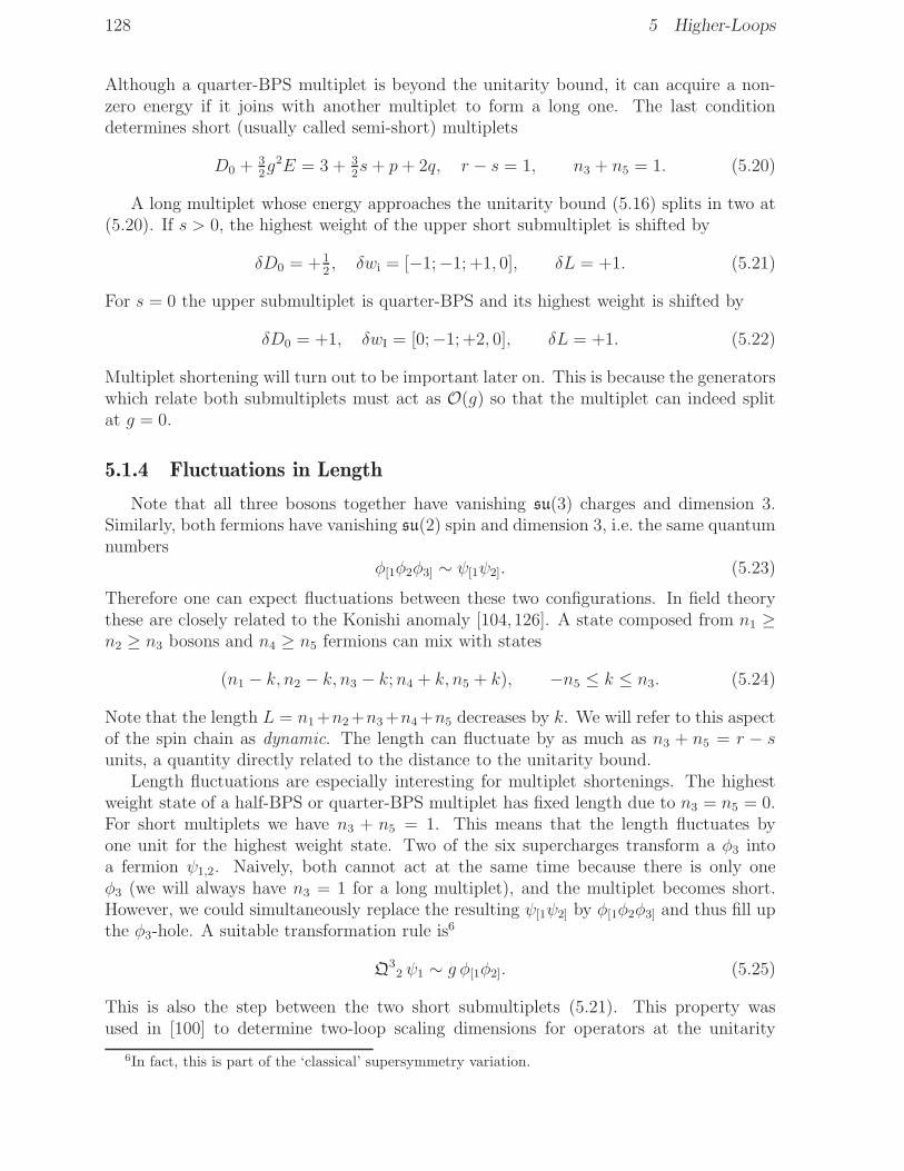
128 5 Higher-Loops
Although a quarter-BPS multiplet is beyond the unitarity bound, it can acquire a non-zero energy if it joins with another multiplet to form a long one. The last conditiondetermines short (usually called semi-short) multiplets
D0 + 32g2E = 3 + 3
2s+ p+ 2q, r − s = 1, n3 + n5 = 1. (5.20)
A long multiplet whose energy approaches the unitarity bound (5.16) splits in two at(5.20). If s > 0, the highest weight of the upper short submultiplet is shifted by
δD0 = +12, δwi = [−1;−1; +1, 0], δL = +1. (5.21)
For s = 0 the upper submultiplet is quarter-BPS and its highest weight is shifted by
δD0 = +1, δwI = [0;−1; +2, 0], δL = +1. (5.22)
Multiplet shortening will turn out to be important later on. This is because the generatorswhich relate both submultiplets must act as O(g) so that the multiplet can indeed splitat g = 0.
5.1.4 Fluctuations in Length
Note that all three bosons together have vanishing su(3) charges and dimension 3.Similarly, both fermions have vanishing su(2) spin and dimension 3, i.e. the same quantumnumbers
φ[1φ2φ3] ∼ ψ[1ψ2]. (5.23)
Therefore one can expect fluctuations between these two configurations. In field theorythese are closely related to the Konishi anomaly [104,126]. A state composed from n1 ≥n2 ≥ n3 bosons and n4 ≥ n5 fermions can mix with states
(n1 − k, n2 − k, n3 − k;n4 + k, n5 + k), −n5 ≤ k ≤ n3. (5.24)
Note that the length L = n1 +n2+n3 +n4+n5 decreases by k. We will refer to this aspectof the spin chain as dynamic. The length can fluctuate by as much as n3 + n5 = r − sunits, a quantity directly related to the distance to the unitarity bound.
Length fluctuations are especially interesting for multiplet shortenings. The highestweight state of a half-BPS or quarter-BPS multiplet has fixed length due to n3 = n5 = 0.For short multiplets we have n3 + n5 = 1. This means that the length fluctuates byone unit for the highest weight state. Two of the six supercharges transform a φ3 intoa fermion ψ1,2. Naively, both cannot act at the same time because there is only oneφ3 (we will always have n3 = 1 for a long multiplet), and the multiplet becomes short.However, we could simultaneously replace the resulting ψ[1ψ2] by φ[1φ2φ3] and thus fill upthe φ3-hole. A suitable transformation rule is6
Q32 ψ1 ∼ g φ[1φ2]. (5.25)
This is also the step between the two short submultiplets (5.21). This property wasused in [100] to determine two-loop scaling dimensions for operators at the unitarity
6In fact, this is part of the ‘classical’ supersymmetry variation.

5.2 Tree-Level 129
bounds from a one-loop field-theory calculation. Note that Q32 annihilates the highest
weight when n4 = 0; we need to apply Q31 first to produce a ψ1. In this case the upper
submultiplet is quarter-BPS (5.22). Furthermore note that when we apply Q31 first, there
are no more φ3’s and ψ2’s left and length fluctuations are ruled out. Therefore, in a BPSor short multiplet we can always find states with fixed length; fluctuations are frozen atthe unitarity bound. In contrast, all states in a multiplet away from the unitarity bound(5.16) are mixtures of states of different lengths.
5.1.5 From N = 4 SYM to su(2|3)
A state of free N = 4 SYM is characterised by the classical dimension D0, the su(2)2
labels [s, s2], the su(4) Dynkin labels [q, p, q2], the u(1) hypercharge B as well as the lengthL. The su(2|3) subsector is obtained by restricting to states with (c.f. Sec. 2.3.4)
D0 = p+ 12q + 3
2q2, s2 = 0. (5.26)
This also implies D0 = B+L. We write these as relations of the corresponding generators
(Rsu(4))44 = 1
2D0, Lα
β = 0, D0 = L+ B. (5.27)
Furthermore, we express the su(4) generator Rsu(4) in terms of an su(3) generator R
(Rsu(4))ab = Ra
b − 16δabD0. (5.28)
Now we can reduce the psu(2, 2|4) algebra as given in App. D.1 to the su(2|3) subsectorand find precisely the su(2|3) relations (c.f. Sec. 5.1.2) if the Hamiltonian H is identifiedwith the anomalous dilatation generator as follows
δD = g2H. (5.29)
As we would like to compare directly to N = 4 SYM, we write one of the generators ofsu(2|3) as D0 + 3
2g2H instead of assigning a new letter.
We note that the states in this subsector are (classically) eighth-BPS in terms ofN = 4SYM (in Sec. 5.6.4 we will present a true eighth-BPS state). Unprotected primary statesof the subsector can therefore not be primary states of psu(2, 2|4). To shift from thecorresponding superconformal primary to the highest weight in the subsector we have toshift by (c.f. Sec. 2.3.4)
δwII = (+1; 0, 0; 0, 0,+2; 0,+1). (5.30)
Note that in terms of the Dynkin labels [s; r; q, p, q2; r2; s2] the last two are zero in thissubsector r2 = s2 = 0. We then simply restrict to the first four labels [s; r; q, p].
5.2 Tree-Level
We would like to construct a representation J(g) of su(2|3)× u(1) on the spin chain.The generators must satisfy the algebra relations
[JM(g), JN(g)
}= FPMN JP (g) (5.31)

130 5 Higher-Loops
with FPMN the structure constants of the symmetry algebra as given in Sec. 5.1.2.Let us illustrate the procedure for the generators at tree-level. At tree-level, composite
states transform in tensor product representations of the fundamental representation 3|2.The generators therefore act on one field at a time. We write down the most general formof generators that respects su(3)× su(2) symmetry
Rab = c1
{ab
}+ c2δ
ab
{cc
},
Lαβ = c3
{αβ
}+ c4δ
αβ
{γγ
},
D0 = c5{aa
}+ c6
{αα
},
(Q0)aα = c7
{aα
},
(S0)αa = c8
{αa
}. (5.32)
The algebra relations have two solutions. One is the trivial solution ck = 0 correspondingto the trivial representation. The other solution requires
c1 = c3 = c5 = 1, c2 = −13, c4 = −1
2, c6 = 3
2, c7 = eiβ1, c8 = e−iβ1 . (5.33)
As expected, we find that the bosons and fermions have dimension 1 and 32, respectively
D0 ={aa
}+ 3
2
{αα
}. (5.34)
The appearance of a free parameter β1 is related to a possible rescaling of the bosons andfermions. This can be represented in terms of a similarity transformation on the algebra
J0 7→ exp(2iβ1D0
)J0 exp
(−2iβ1D0
). (5.35)
Obviously, the algebra relations in Sec. 5.1.2 are invariant under such a transformation.The only other su(3)× su(2) invariant similarity transformation besides (5.35) is
J0 7→ exp(iβ2L
)J0 exp
(−iβ2L
), (5.36)
where L is the length operator
L ={aa
}+{αα
}or simply L =
{ ··}. (5.37)
The transformation (5.36) is trivial and does not give rise to a new parameter at tree-levelbecause the length is conserved there
[L, J0] = 0. (5.38)
5.3 One-Loop
In this section we construct deformations of the algebra generators J(g) obeying thealgebra relations in Sec. 5.1.2. Here, we will proceed up to O(g) for the deformations ofthe Hamiltonian H(g). This can still be done conveniently by hand without the help ofcomputer algebra systems. This section is meant to illustrate the methods of this chapterin a simple context before we proceed to higher-loops in the sections to follow.
The most important one of the algebra relations is the invariance of the interactionHamiltonian
[JM(g),H(g)] = 0. (5.39)
Moreover we will assume the su(2), su(3) rotation generators Rab and Lα
β to receive nocorrections. This is natural, for the rotation symmetries are preserved by the quantisationprocedure.

5.3 One-Loop 131
Figure 5.2: The structures for the construction of H0. Straight and zigzag lines correspond tobosons and fermions, respectively.
5.3.1 Pre-Leading Order
Let us restrict (5.39) to its leading order
[J0,Hl] = 0, (5.40)
in other words, the leading order of the Hamiltonian at some O(gl) is conserved by theclassical algebra. The leading order for H will be l = 0 and we shall now exclude acorrection to H at order l = −1 7 by representation theory in analogy to Sec. 3.1.3: Atthis order the interactions have three legs and the possible ways to distribute them amongthe in and out channels are
{ ·ABC
},{
CAB
},{BCA
},{ABC
·}. (5.41)
The indices cannot be contracted fully, hence there is no invariant interaction at thisorder. In other words there is no common irreducible representation of the free algebraamong the in and the out channel
V0F6∈ V3
F, V1
F6∈ V2
F. (5.42)
5.3.2 Leading Order
A similar argument is used to show that at leading order we must evenly distributethe four fields among the in and out channel, i.e.
V0F6∈ V4
F, V1
F6∈ V3
F, but V2
F= V2
F. (5.43)
The most general form of H0, expressed as an action on bosons (a, b) and fermions (α, β)is therefore
H0 = c1{abab
}+ c2
{aβaβ
}+ c′2
{αbαb
}+ c3
{αβαβ
}
+ c4{abba
}+ c5
{aββa
}+ c′5
{αbbα
}+ c6
{αββα
}, (5.44)
see also Fig. 5.2. First of all we demand that H0 conserves parity (5.10),
pH0 p−1 = H0. (5.45)
As can be seen easily, this requires
c2 = c′2, c5 = c′5. (5.46)
7Note that H is shifted by two orders in perturbation theory due to δD = g2H. It therefore makessense to consider H−1 = D1.
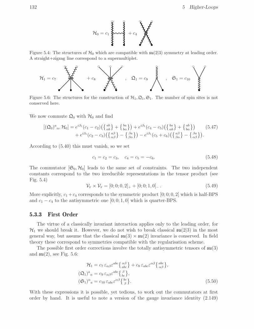
132 5 Higher-Loops
H0 = c1 + c4
Figure 5.4: The structures of H0 which are compatible with su(2|3) symmetry at leading order.A straight+zigzag line correspond to a supermultiplet.
H1 = c7 + c8 , Q1 = c9 , S1 = c10
Figure 5.6: The structures for the construction of H1,Q1,S1. The number of spin sites is notconserved here.
We now commute Q0 with H0 and find
[(Q0)aα,H0] = eiβ1(c1 − c2)
({abαb
}+{babα
})+ eiβ1(c4 − c5)
({baαb
}+{abbα
})(5.47)
+ eiβ1(c2 − c3)({
aβαβ
}−{βaβα
})− eiβ1(c5 + c6)
({aββα
}−{βaαβ
}).
According to (5.40) this must vanish, so we set
c1 = c2 = c3, c4 = c5 = −c6. (5.48)
The commutator [S0,H0] leads to the same set of constraints. The two independentconstants correspond to the two irreducible representations in the tensor product (seeFig. 5.4)
VF × VF = [0; 0; 0, 2]+ + [0; 0; 1, 0]− . (5.49)
More explicitly, c1 + c4 corresponds to the symmetric product [0; 0; 0, 2] which is half-BPSand c1 − c4 to the antisymmetric one [0; 0; 1, 0] which is quarter-BPS.
5.3.3 First Order
The virtue of a classically invariant interaction applies only to the leading order, forH1 we should break it. However, we do not wish to break classical su(2|3) in the mostgeneral way, but assume that the classical su(3)× su(2) invariance is conserved. In fieldtheory these correspond to symmetries compatible with the regularisation scheme.
The possible first order corrections involve the totally antisymmetric tensors of su(3)and su(2), see Fig. 5.6:
H1 = c7 εαβεabc{αβabc
}+ c8 εabcε
αβ{abcαβ
},
(Q1)aα = c9 εαβε
abc{βbc
},
(S1)αa = c10 εabcε
αβ{bcβ
}. (5.50)
With these expressions it is possible, yet tedious, to work out the commutators at firstorder by hand. It is useful to note a version of the gauge invariance identity (2.149)
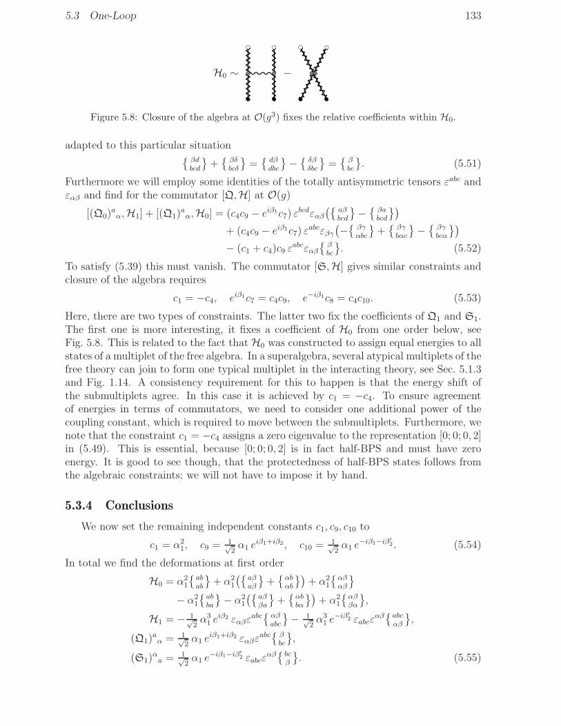
5.3 One-Loop 133
H0 ∼ −
Figure 5.8: Closure of the algebra at O(g3) fixes the relative coefficients within H0.
adapted to this particular situation{βdbcd
}+{βδbcδ
}={dβdbc
}−{δβδbc
}={βbc
}. (5.51)
Furthermore we will employ some identities of the totally antisymmetric tensors εabc andεαβ and find for the commutator [Q,H] at O(g)
[(Q0)aα,H1] + [(Q1)
aα,H0] = (c4c9 − eiβ1c7) ε
bcdεαβ({
aβbcd
}−{βabcd
})
+ (c4c9 − eiβ1c7) εabcεβγ
(−{βγαbc
}+{βγbαc
}−{βγbcα
})
− (c1 + c4)c9 εabcεαβ
{βbc
}. (5.52)
To satisfy (5.39) this must vanish. The commutator [S,H] gives similar constraints andclosure of the algebra requires
c1 = −c4, eiβ1c7 = c4c9, e−iβ1c8 = c4c10. (5.53)
Here, there are two types of constraints. The latter two fix the coefficients of Q1 and S1.The first one is more interesting, it fixes a coefficient of H0 from one order below, seeFig. 5.8. This is related to the fact that H0 was constructed to assign equal energies to allstates of a multiplet of the free algebra. In a superalgebra, several atypical multiplets of thefree theory can join to form one typical multiplet in the interacting theory, see Sec. 5.1.3and Fig. 1.14. A consistency requirement for this to happen is that the energy shift ofthe submultiplets agree. In this case it is achieved by c1 = −c4. To ensure agreementof energies in terms of commutators, we need to consider one additional power of thecoupling constant, which is required to move between the submultiplets. Furthermore, wenote that the constraint c1 = −c4 assigns a zero eigenvalue to the representation [0; 0; 0, 2]in (5.49). This is essential, because [0; 0; 0, 2] is in fact half-BPS and must have zeroenergy. It is good to see though, that the protectedness of half-BPS states follows fromthe algebraic constraints; we will not have to impose it by hand.
5.3.4 Conclusions
We now set the remaining independent constants c1, c9, c10 to
c1 = α21, c9 = 1√
2α1 e
iβ1+iβ2, c10 = 1√2α1 e
−iβ1−iβ′2 . (5.54)
In total we find the deformations at first order
H0 = α21
{abab
}+ α2
1
({aβaβ
}+{αbαb
})+ α2
1
{αβαβ
}
− α21
{abba
}− α2
1
({aββa
}+{αbbα
})+ α2
1
{αββα
},
H1 = − 1√2α3
1 eiβ2 εαβε
abc{αβabc
}− 1√
2α3
1 e−iβ′
2 εabcεαβ{abcαβ
},
(Q1)aα = 1√
2α1 e
iβ1+iβ2 εαβεabc{βbc
},
(S1)αa = 1√
2α1 e
−iβ1−iβ′2 εabcε
αβ{bcβ
}. (5.55)

134 5 Higher-Loops
Let us discuss the free parameters. The parameter β ′2 will in fact be determined by a
constraint from fourth order, see the following section: c9c10 = 12c1 or
β ′2 = β2. (5.56)
As shown in (5.35,5.36), the coefficients β1,2 correspond to a similarity transformation ofthe algebra
J0 7→ exp(2iβ1D0 + iβ2L
)J0 exp
(−2iβ1D0 − iβ2L
). (5.57)
The algebra relations (5.31) are invariant under similarity transformations, so β1,2 cantake arbitrary values. For convenience, we might fix a gauge and set β1 = β2 = 0, but wewill refrain from doing that here. Last but not least, the parameter α1 corresponds to arescaling of the coupling constant
g 7→ α1 g. (5.58)
The algebra relations (5.31) are also invariant under this redefinition.In a real form of the algebra we get a few additional constraints. There, the algebra
should be self-adjoint which imposes some reality constraint on α1, β1,2. For a real su(2|3)they have to be real and α2
1 needs to be positive. This ensures positive planar energies asrequired by the unitarity bound.
In conclusion we have found that the deformations of the generators are uniquely fixedat one-loop. Note that H0 agrees with the complete one-loop dilatation operator foundin Ch. 3. Here, it is understood that some parameters cannot be fixed due to symmetriesof the algebra relations. In determining the coefficients we saw that [H(g), J(g)] = 0at order O(g2ℓ−2) makes the ℓ-loop energy shift agree within short multiplets, whereasO(g2ℓ−1) joins up short multiplets into long multiplets. Note that the anticommutatorof supercharges at first order is trivially satisfied due to the flavours of incoming andoutgoing fields
{(S1)αa, (Q0)
bβ}+ {(S0)
αa, (Q1)
bβ} = 0 = 1
2δbaδ
αβH−1. (5.59)
5.4 Two-Loops
In this section we will discuss the restrictions from the algebra at two-loops, i.e. upto third order. The steps are straightforward, but involve very lengthy expressions. Wehave relied on the algebra system Mathematica to perform the necessary computations.
5.4.1 Structures
At second order we need to determine H2,Q2,S2. For H2 the su(3)× su(2) invariantinteractions which preserve the dimension also preserve the number of fields, i.e. threefields are mapped into three fields. Similarly, for Q2,S2 we need two fields going into twofields
H2 ∼{A1A2A3
B1B2B3
}, Q2,S2 ∼
{A1A2
B1B2
}. (5.60)
It is an easy exercise to count the number of structures in H2,Q2,S2. For H2 there 23 = 8ways to determine the statistics of A1A2A3 and 3! = 6 ways to permute the fields (eachA must be contracted to one of the B’s). In total there are 6 · 8 = 48 structures for H2

5.4 Two-Loops 135
and 8 for Q2,S2 each. We now demand parity conservation. This restricts the numberof independent structures to 28 and 4 for H2 and Q2,S2, respectively.
At third order we need to determine H3,Q3,S3. Like H1,Q1,S1, all of these involvethe totally antisymmetric tensors for su(3), su(2) and change the number of fields by one.Counting of independent structures is also straightforward, we find 48 for H3 and 12 forQ3,S3 each. Parity conservation halves each of these numbers.
5.4.2 Coefficients
Now we demand that energy shifts are conserved at third order
[Qaα,H] = [Sα
a,H] = O(g4). (5.61)
This fixes the remaining coefficient β ′2 at first order (5.56) and many coefficients at second
and third order. The anticommutator of supercharges
{Sαa,Q
bβ} = δbaL
αβ + δαβRb
a + δbaδαβ (1
3D0 + 1
2g2H) +O(g4) (5.62)
does not lead to additional constraints. The resulting deformations of the generators upto second order are presented in Tab. 5.2. In the remainder of this subsection we shalldiscuss the undetermined coefficients α, γ, δ and we shall find an explanation for each ofthem.
• Firstly, the constants δ1,2 multiply a structure which has a spectator leg on either sideof the interaction
{ A1...AEiC
B1...BEoC
}− (−1)C(A1...AEi
B1...BEo ){ CA1...AEi
CB1...BEo
}, (5.63)
such that both interactions cancel out in a cyclic state.
• Secondly, the constant δ3 multiplies a structure which is zero due to an su(2) identity.We cannot antisymmetrise more than two fundamental representations of su(2)
{αβγ[αβγ]
}= 0. (5.64)
• Thirdly, we can use a similarity transformation to modify the generators
J(g) 7→ T (g) J(g)T (g)−1. (5.65)
In Sec. 5.3.4, we have used a transformation which is independent of the couplingconstant, here we consider a transformation T (g) = 1 + g2T2 + . . . proportional tog2. For consistency with the algebra, the transformation will have to be su(3)× su(2)invariant and preserve the dimension as well as parity. Also, according to Sec. 2.6.2,it should involve four fields. These are exactly the requirements for the form of H0,the 6 independent structures are given in (5.44,5.45). Out of these six, there are twospecial combinations: One of them is H0 itself and the other one is equivalent to thelength operator
L ={abab
}+{aβaβ
}+{αbαb
}+{αβαβ
}(5.66)

136 5 Higher-Loops
Rab =
{ab
}− 1
3δab{cc
},
Lαβ =
{αβ
}− 1
2δαβ{γγ
},
D0 ={aa
}+ 3
2
{αα
},
H0 = α21
{abab
}+ α2
1
({aβaβ
}+{αbαb
})+ α2
1
{αβαβ
}
− α21
{abba
}− α2
1
({aββa
}+{αbbα
})+ α2
1
{αββα
},
H1 = − 1√2α3
1 eiβ2 εαβε
abc{αβabc
}− 1√
2α3
1 e−iβ2 εabcε
αβ{abcαβ
},
H2 = (−2α41 + 2α1α3)
{abcabc
}+ (−1
2α4
1 + 2α1α3 + δ3){αβγαβγ
}
+ (12α4
1 + 2α1α3 + 2δ2){aβcaβc
}+ (−4α4
1 + 2α1α3 − 2δ2){αbγαbγ
}
+ (−114α4
1 + 2α1α3 − δ2)({
abγabγ
}+{αbcαbc
})+ (2α1α3 + δ2)
({aβγaβγ
}+{αβcαβc
})
+ (32α4
1 − α1α3)({
abcbac
}+{abcacb
})+ (α4
1 − α1α3)({
abγbaγ
}+{αbcαcb
})
+ (54α4
1 − α1α3 + iα21γ3 + iδ1)
({αbcbαc
}+{abγaγb
})
+ (54α4
1 − α1α3 − iα21γ3 − iδ1)
({aβcβac
}+{aβcacβ
})
+ (α41 − α1α3 + iδ1)
({αbγbαγ
}+{αbγαγb
})
+ (α41 − α1α3 − iδ1)
({aβγβaγ
}+{αβcαcβ
})
+ (−74α4
1 + α1α3)({
αβcβαc
}+{aβγaγβ
})+ (−7
4α4
1 + α1α3 − δ3)({
αβγβαγ
}+{αβγαγβ
})
− 12α4
1
({abccab
}+{abcbca
})+ δ3
({αβγγαβ
}+{αβγβγα
})
+ (−14α4
1 + iα21γ1)
({αbccαb
}+{abγbγa
})+ (1
4α4
1 + iα21γ2)
({aβγγaβ
}+{αβcβcα
})
+ (−14α4
1 − iα21γ1)
({aβccaβ
}+{aβcβca
})+ (1
4α4
1 − iα21γ2)
({αbγγαb
}+{αbγbγα
})
− 12α4
1
({abγγba
}+{αbccbα
})+ 1
2α4
1
{αbγγbα
}− δ3
{αβγγβα
}
+ 32α4
1
([αβαβ
]−[αββα
]),
(Q0)aα = eiβ1
{aα
},
(Q1)aα = 1√
2α1 e
iβ1+iβ2εαβεabc{βbc
},
(Q2)aα = eiβ1(1
4α2
1 − i12γ3 + i12γ4)({
abαb
}+{babα
})+ eiβ1(1
2iγ3 + 1
2iγ4)
({aβαβ
}−{βaβα
})
+ eiβ1(−14α2
1 − iγ1)({
abbα
}+{baαb
})+ eiβ1(1
4α2
1 + iγ2)({
aββα
}−{βaαβ
}),
(S0)αa = e−iβ1
{αa
},
(S1)αa = 1√
2α1 e
−iβ1−iβ2εabcεαβ{bcβ
},
(S2)αa = e−iβ1(1
4α2
1 + 12iγ3 − 1
2iγ4)
({αbab
}+{bαba
})+ e−iβ1(−1
2iγ3 − 1
2iγ4)
({αβaβ
}−{βαβa
})
+ e−iβ1(−14α2
1 + iγ1)({
αbba
}+{bαab
})+ e−iβ1(1
4α2
1 − iγ2)(−{αββa
}+{βαaβ
}).
Table 5.2: Two-loop deformations of the generators

5.4 Two-Loops 137
up to gauge transformations. The similarity transformation amounts to adding com-mutators with H0,Q0,S0
H2 7→ H2 + [T2,H0], J2 7→ J2 + [T2, J0]. (5.67)
These commutators vanish for H0 and L[H0, J0] = [L, J0] = [H0,H0] = [L,H0] = 0. (5.68)
In other words, conjugation with g2H0 and g2L will have no effect on H2,Q2,S2. Theremaining four structures in (5.44,5.45) do not commute with H0,Q0,S0 and amountto the constants γ1,2,3,4. Note that γ4 is related to the structure D0 and does notappear in H2 because of [D0,H0] = 0.
• Finally, we are allowed to perform a transformation of the coupling constant
J(g) 7→ J(f(g)). (5.69)
If we use the function f(g) = α1g + α3g3 we find that
H2 7→ α41H2 + 2α1α3H0, (5.70)
which explains the degree of freedom α3.
5.4.3 Short States and Wrapping Interactions
The second order interactions H2 act on three fields. We should also determine itsaction on the states of length two8
O(ab) = |ab〉 = Trφaφb, Oaβ = |aβ〉 = Trφaψβ , O1 = εαβ|αβ〉 = εαβ Trψαψβ . (5.71)
Together, these form the protected half-BPS multiplet [0; 0; 0, 2]. It is therefore reassuringto see thatO(ab) andOaβ are annihilated byH0,H1; just as well they should be annihilatedby H2. For O1 the situation is different: It is annihilated by H0, but H1 produces theoperator
O2 = εabc|abc〉 = εabc Trφaφbφc. (5.72)
The action of H(g) on these two operators up to second order is given by
H(g)
(O1
O2
)=
(ǫg2 −2
√2 eiβ2α3
1g
−9√
2 eiβ2e−iβ2α31g 6α2
1 − 18α21g
2 + 12α1α3g2
)(O1
O2
), (5.73)
where we have assumed that H2O1 = ǫO1. The eigenvalues of this matrix at fourth orderare given by
E1 = ǫg2 − 6α41g
2, E2 = 6α21 − 12α4
1g2 + 12α1α3g
2. (5.74)
Due to its half-BPS nature, the energy of the diagonalised O1 must be exactly zero,E1 = 0, and we set
ǫ = 6α41. (5.75)
The second order Hamiltonian for states of length two should thus annihilate the statesO(ab),Oaβ and yield 6α4
1O1 when acting onO1. This is achieved by a wrapping interaction,c.f. Sec. 2.6.3,
H2 = . . .+ 32α4
1
([αβαβ
]−[αββα
]). (5.76)
8Length-one states are U(1) fields and do not interact at all.

138 5 Higher-Loops
5.4.4 Conclusions
We see that for all free parameters in Tab. 5.2 there is an associated symmetry of thealgebra relations and we can say that the two-loop contribution is uniquely fixed. The onlyparameter that influences energies is α3; we cannot remove it by algebraic considerations.The parameters γ1,2,3,4 rotate only the eigenstates. Finally, the parameters δ1,2,3 are thereonly because we were not careful enough in finding independent structures (for H2 thereare only 25 = 28− 3 independent structures). They have no effect at all.
5.5 Three-Loops
For the fourth order contributions H4,Q4,S4 we find in total 208 + 56 + 56 parityconserving structures; they all conserve the number of fields9. Of these only 173+32+32are independent due to identities as discussed above. We impose the constraint (5.39) atfourth order
[Q,H] = [S,H] = O(g5) (5.77)
and find that the algebra relations fix 202 coefficients (plus one coefficient at third order).This leaves 35 free coefficients. The anticommutator of supercharges (5.9) at fourth order
{Sαa,Q
bβ} = δbaL
αβ + δαβRb
a + δbaδαβ (1
3D0 + 1
2g2H) +O(g5) (5.78)
is satisfied automatically.As we have learned above, the commutators at fourth order are not sufficient to ensure
consistency for splitting multiplets at the unitarity bound, we should also consider fifthorder. To perform those commutators would be even harder. We therefore consider a setof probe multiplets at the unitarity bound. By requiring that the three-loop energy shiftscoincide within submultiplets we are able to fix another 8 coefficients.
Still this leaves 27 coefficients to be fixed, however, almost all of them rotate thespace of states. Experimentally, we found that only 4 coefficients affect the energies. Theremaining 23 coefficients can be attributed to similarity transformations. As before, thenumber of similarity transformations equals the number of structures for H2, i.e. 25. Thismeans that there must be 2 commuting generators which are readily found to be g4H0
and g4L. We summarise our findings concerning the number of coefficients in Tab. 5.4.The symmetries indicated in the table refer to L (which is conserved at leading order butbroken at first order, hence the −1 at k = 1), g2L (broken at third order), g2H, g4L (willbreak at fifth order) and g4H. This sequence of symmetries will continue at higher orders,but there will be additional ones due to integrability, see Sec. 6.1.4.
Let us now discuss the relevant coefficients. One coefficient is due to a redefinitionof the coupling constant and cannot be fixed algebraically. To constrain the other threewe will need further input. Unfortunately, the resulting generators are too lengthy tobe displayed here. Instead, let us have a look at the set of totally bosonic states. Inthis subsector (which is closed only when further restricted to two flavours, i.e. the su(2)subsector) H4 is presented in Tab. 5.6.
The coefficients in Tab. 5.6 can be understood as follows. The coefficients σ1,2,3,4 arerelevant. One of them, σ1, multiplies the structure H0 (up to spectator legs) and therefore
9At sixth order the number of fields can be changed by two using four antisymmetric tensors.
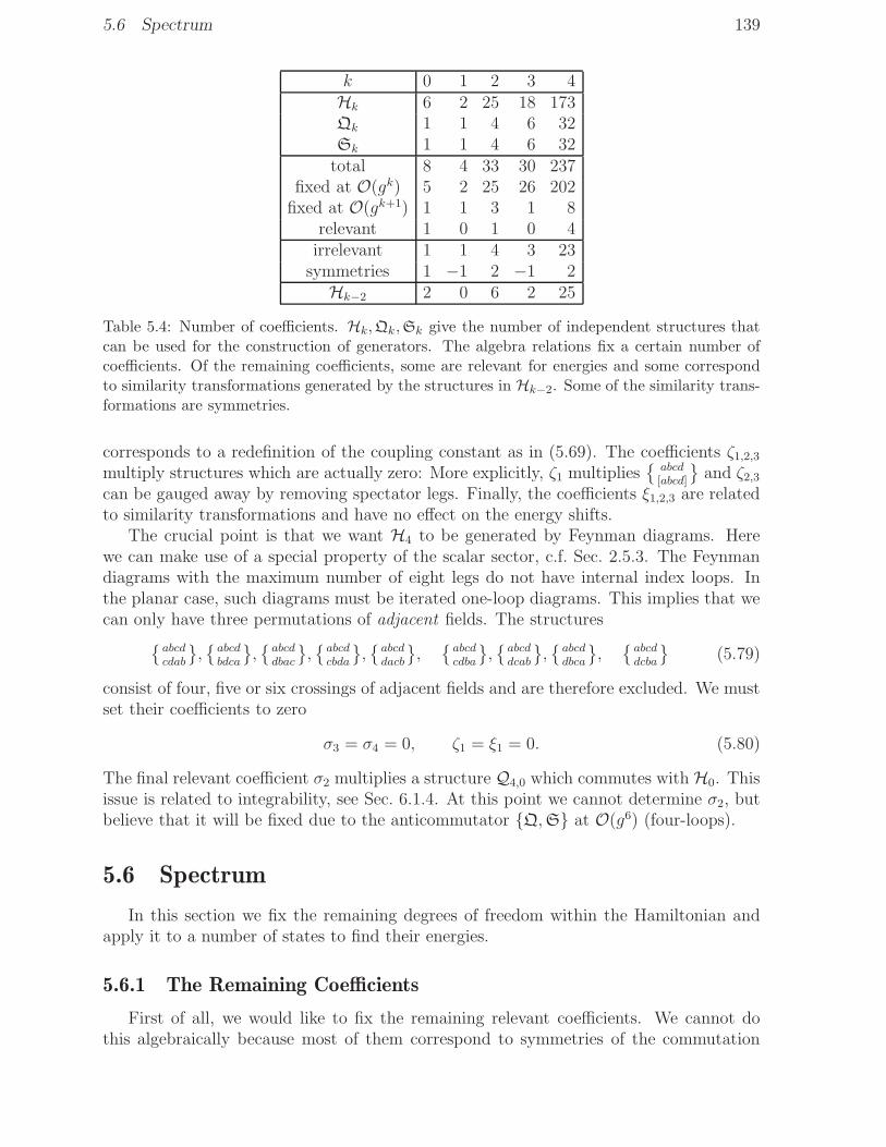
5.6 Spectrum 139
k 0 1 2 3 4Hk 6 2 25 18 173Qk 1 1 4 6 32Sk 1 1 4 6 32
total 8 4 33 30 237fixed at O(gk) 5 2 25 26 202
fixed at O(gk+1) 1 1 3 1 8relevant 1 0 1 0 4irrelevant 1 1 4 3 23
symmetries 1 −1 2 −1 2Hk−2 2 0 6 2 25
Table 5.4: Number of coefficients. Hk,Qk,Sk give the number of independent structures thatcan be used for the construction of generators. The algebra relations fix a certain number ofcoefficients. Of the remaining coefficients, some are relevant for energies and some correspondto similarity transformations generated by the structures in Hk−2. Some of the similarity trans-formations are symmetries.
corresponds to a redefinition of the coupling constant as in (5.69). The coefficients ζ1,2,3multiply structures which are actually zero: More explicitly, ζ1 multiplies
{abcd[abcd]
}and ζ2,3
can be gauged away by removing spectator legs. Finally, the coefficients ξ1,2,3 are relatedto similarity transformations and have no effect on the energy shifts.
The crucial point is that we want H4 to be generated by Feynman diagrams. Herewe can make use of a special property of the scalar sector, c.f. Sec. 2.5.3. The Feynmandiagrams with the maximum number of eight legs do not have internal index loops. Inthe planar case, such diagrams must be iterated one-loop diagrams. This implies that wecan only have three permutations of adjacent fields. The structures
{abcdcdab
},{abcdbdca
},{abcddbac
},{abcdcbda
},{abcddacb
},{abcdcdba
},{abcddcab
},{abcddbca
},{abcddcba
}(5.79)
consist of four, five or six crossings of adjacent fields and are therefore excluded. We mustset their coefficients to zero
σ3 = σ4 = 0, ζ1 = ξ1 = 0. (5.80)
The final relevant coefficient σ2 multiplies a structure Q4,0 which commutes with H0. Thisissue is related to integrability, see Sec. 6.1.4. At this point we cannot determine σ2, butbelieve that it will be fixed due to the anticommutator {Q,S} at O(g6) (four-loops).
5.6 Spectrum
In this section we fix the remaining degrees of freedom within the Hamiltonian andapply it to a number of states to find their energies.
5.6.1 The Remaining Coefficients
First of all, we would like to fix the remaining relevant coefficients. We cannot dothis algebraically because most of them correspond to symmetries of the commutation
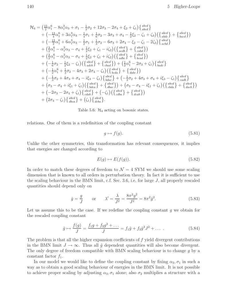
140 5 Higher-Loops
H4 =(
152α6
1 − 8α31α3 + σ1 − 1
3σ2 + 12σ3 − 2σ4 + ξ2 + ζ1
){abcdabcd
}
+(−13
4α6
1 + 3α31α3 − 1
4σ1 + 1
6σ2 − 3σ3 + σ4 − 1
2ξ2 − ζ1 + ζ3
)({abcdabdc
}+{abcdbacd
})
+(−13
2α6
1 + 6α31α3 − 1
2σ1 + 1
3σ2 − 6σ3 + 2σ4 − ξ2 − ζ1 − 2ζ3
){abcdacbd
}
+(
32α6
1 − α31α3 − σ4 + 1
2ξ2 + ζ1 − iζ2
)({abcdacdb
}+{abcdcabd
})
+(
32α6
1 − α31α3 − σ4 + 1
2ξ2 + ζ1 + iζ2
)({abcdadbc
}+{abcdbcad
})
+(−1
6σ2 − 1
2ξ2 − ζ1
)({abcdadcb
}+{abcdcbad
})+(
12α6
1 − 2σ3 + ζ1){
abcdbadc
}
+(−1
2α6
1 + 13σ2 − 4σ3 + 2σ4 − ζ1
)({abcdbcda
}+{abcddabc
})
+(−1
3σ2 + 4σ3 + σ4 − iξ3 − ζ1
){abcdbdac
}+(−1
3σ2 + 4σ3 + σ4 + iξ3 − ζ1
){abcdcadb
}
+(σ3 − σ4 + iξ1 + ζ1
)({abcdbdca
}+{abcddbac
})+(σ3 − σ4 − iξ1 + ζ1
)({abcdcbda
}+{abcddacb
})
+(−2σ3 − 2σ4 + ζ1
){abcdcdab
}+(−ζ1
)({abcdcdba
}+{abcddcab
})
+(2σ4 − ζ1
){abcddbca
}+(ζ1){
abcddcba
}.
Table 5.6: H4 acting on bosonic states.
relations. One of them is a redefinition of the coupling constant
g 7→ f(g). (5.81)
Unlike the other symmetries, this transformation has relevant consequences, it impliesthat energies are changed according to
E(g) 7→ E(f(g)). (5.82)
In order to match these degrees of freedom to N = 4 SYM we should use some scalingdimension that is known to all orders in perturbation theory. In fact it is sufficient to usethe scaling behaviour in the BMN limit, c.f. Sec. 3.6, i.e. for large J , all properly rescaledquantities should depend only on
g =g
Jor λ′ =
λ
J2=
8π2g2
J2= 8π2g2. (5.83)
Let us assume this to be the case. If we redefine the coupling constant g we obtain forthe rescaled coupling constant
g 7→ f(g)
J=f1g + f3g
3 + . . .
J= f1g + f3g
3J2 + . . . . (5.84)
The problem is that all the higher expansion coefficients of f yield divergent contributionsin the BMN limit J → ∞. Thus all g dependent quantities will also become divergent.The only degree of freedom compatible with BMN scaling behaviour is to change g by aconstant factor f1.
In our model we would like to define the coupling constant by fixing α3, σ1 in such away as to obtain a good scaling behaviour of energies in the BMN limit. It is not possibleto achieve proper scaling by adjusting α3, σ1 alone; also σ2 multiplies a structure with a

5.6 Spectrum 141
wrong scaling. This is fortunate, because it allows us to determine σ2 as well, in total wefind
α3 = 0, σ1 = 0, σ2 = 0. (5.85)
Afterwards we can only change α1. This final degree of freedom is eliminated by a singleknown scaling dimension, e.g. the one of the Konishi multiplet (2.20) E0 = 6, or usingthe quantitative BMN energy formula (3.99). It fixes α1 to unity
α1 = 1. (5.86)
We conclude that the planar three-loop Hamiltonian is uniquely fixed by the symmetryalgebra, field theory and the BMN scaling behaviour.10 Together with the fact that thismodel is a closed subsector of N = 4 SYM we have derived the planar dilatation generatorin the su(2|3) subsector at three-loops. Similarly, this model is a closed subsector of theBMN matrix model and the two Hamiltonians must agree up to three loops (after aredefinition of the coupling constant and provided that the BMN matrix model has aBMN limit). This is indeed the case as shown in [79].
5.6.2 Lowest-Lying States
We are now ready to compute numerical values for some energies. For this we shouldconsider the charges D0, s, p, q, L of a state and compute the number of constituent fieldsaccording to (5.15). These are arranged within a trace in all possible ways
En = (Trφn1
1 φn2
2 φn3
3 ψn4
1 ψn5
2 , . . .). (5.87)
Note that the length L is not a good quantum number at O(g), so we must include statesof all admissible lengths in (5.87). In practice this means that we may replace a completeset of bosons φ1φ2φ3 by a complete set of fermions ψ1ψ2, (5.23). Due to conservationof charges, the Hamiltonian closes on this set of states and we can evaluate its matrixelements11
H(g) Ei = Ej Hji(g). (5.88)
It is a straightforward task to find the eigenvalues and their perturbations
H(g) = H0 + V (g), with V = O(g). (5.89)
Diagonalising the leading order matrix H0 is a non-linear problem. The resulting eigen-values represent the one-loop energies E0. Now we pick an eigenvalue e = E0 of H0 andconsider the subspace of states with energy e. The higher-order energy shifts are given by(in contrast to the formula in [79] V ′ was constructed such that conjugation symmetry is
10Without BMN scaling the constants α1, α3, σ1, σ2 remain unknown. However, α1, α3, σ1 are relatedto a redefinition of the coupling constant and, as we shall see in Sec. 6.1.4, there is a natural explanationfor σ2 in terms of integrability. It therefore makes sense to say that the Hamiltonian is uniquely fixed(up to symmetries) even without making use of BMN scaling.
11Although the Hilbert space is infinite-dimensional, the Hamiltonian acts on a space of fixed dimensionD0. Therefore the matrix Hj
i(g) has a finite size.

142 5 Higher-Loops
preserved)
V ′ =∑
eΠe
[V + V ∆eV +
(V ∆eV ∆eV − 1
2V ∆2
eV ΠeV − 12V ΠeV ∆
2eV)
+ V ∆eV ∆eV ∆eV − 12V ∆2
eV ΠeV ∆eV − 12V ∆eV ΠeV ∆
2eV
− 12V ∆2
eV ∆eV ΠeV − 12V ΠeV ∆eV ∆
2eV (5.90)
− 12V ∆eV ∆
2eV ΠeV − 1
2V ΠeV ∆
2eV ∆eV
+ 13V ∆3
eV ΠeV ΠeV + 13V ΠeV ∆
3eV ΠeV + 1
3V ΠeV ΠeV ∆
3eV + . . .
]Πe.
The propagator ∆e is given by
∆e =1−Πe
e−H0(5.91)
and Πe projects to the subspace with leading correction e. If there is only a single statewith one-loop energy e, (5.90) gives its higher order corrections. For degenerate statesat one-loop, (5.89,5.90) must be applied iteratively until the resulting matrix V ′ becomesdiagonal12.
Next, it is important to know the multiplets of states. In the interacting theory thereare two types of single-trace multiplets, half-BPS and long ones. The half-BPS multipletsare easily identified, there is one multiplet with labels
D0 = L = p, E = 0, [0; 0; 0, p], P = (−1)p (5.92)
for each p, they receive no corrections to their energy. Long multiplets are not so easyto find. By means of a C++ computer programme we have constructed the spectrum ofall states explicitly (up to some energy bound) and iteratively removed the multipletscorresponding to the leftover highest weight state (this ‘sieve’ algorithm, also reminiscentof the standard algorithm for division, is described in more detail in [105,106]). For a setof states with given charges as in (5.87) this also tells us how many representatives thereare from each of the multiplets and allows us to identify the energy we are interested in.
Finally, to obtain the energy shift of a given multiplet, a lot of work can be savedby choosing a suitable representative. Resolving the mixing problem for the highestweight state is usually more involved than for a descendant. For instance, highest weightstates involve all three flavours of bosons, n1, n2, n3 ≥ 1. This increases the number ofpermutations in (5.87) and also gives rise to mixing between states of different lengths.The matrix Hm
n will be unnecessarily large. If, instead, one applies three supergeneratorsQ1
4Q24Q
34, i.e.
n1 7→ n1 − 1, n2 7→ n2 − 1, n3 7→ n3 − 1, n4 7→ n4 + 3, (5.93)
the state becomes more uniform. This decreases the number of permutations and, in thecase of multiplets at the unitarity bound (5.16), mixing between states of different lengthsis prevented due to n3 = n5 = 0.
We summarise our findings for states of dimension D0 ≤ 8.5 in Tab. 5.8. We havelabelled the states by their dimension D0, classical su(2|3) Dynkin labels, and classicallength L. For each multiplet we have given its energy E = E0 + g2E2 + g4E4 +O(g6) up
12In principle it could happen that states with equal leading order energy e have matrix elements atO(g). In this case the energy would have an expansion in terms of g ∼
√λ instead of g2 ∼ λ similar to
the peculiarities noticed in [38]. It would be interesting to see if this does indeed happen or, if not, why?
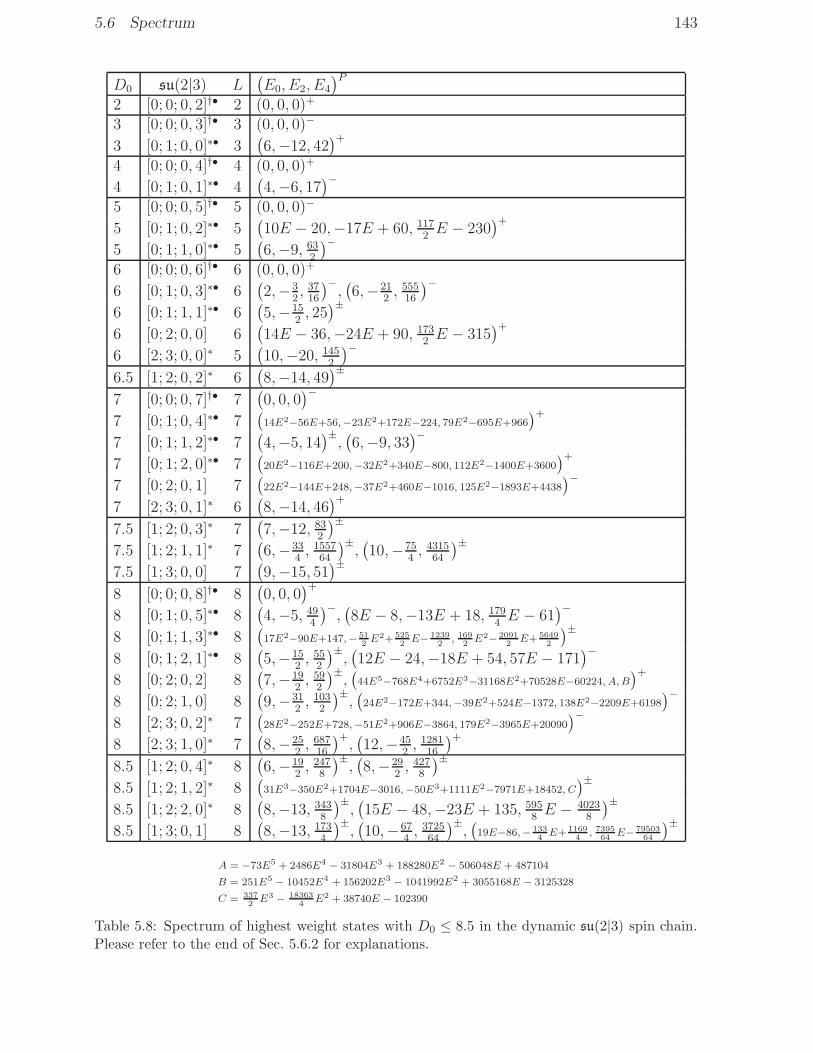
5.6 Spectrum 143
D0 su(2|3) L(E0, E2, E4
)P
2 [0; 0; 0, 2]†• 2 (0, 0, 0)+
3 [0; 0; 0, 3]†• 3 (0, 0, 0)−
3 [0; 1; 0, 0]∗• 3(6,−12, 42
)+
4 [0; 0; 0, 4]†• 4 (0, 0, 0)+
4 [0; 1; 0, 1]∗• 4(4,−6, 17
)−
5 [0; 0; 0, 5]†• 5 (0, 0, 0)−
5 [0; 1; 0, 2]∗• 5(10E − 20,−17E + 60, 117
2E − 230
)+
5 [0; 1; 1, 0]∗• 5(6,−9, 63
2
)−
6 [0; 0; 0, 6]†• 6 (0, 0, 0)+
6 [0; 1; 0, 3]∗• 6(2,−3
2, 37
16
)−,(6,−21
2, 555
16
)−
6 [0; 1; 1, 1]∗• 6(5,−15
2, 25)±
6 [0; 2; 0, 0] 6(14E − 36,−24E + 90, 173
2E − 315
)+
6 [2; 3; 0, 0]∗ 5(10,−20, 145
2
)−
6.5 [1; 2; 0, 2]∗ 6(8,−14, 49
)±
7 [0; 0; 0, 7]†• 7(0, 0, 0
)−
7 [0; 1; 0, 4]∗• 7(14E2−56E+56,−23E2+172E−224, 79E2−695E+966
)+
7 [0; 1; 1, 2]∗• 7(4,−5, 14
)±,(6,−9, 33
)−
7 [0; 1; 2, 0]∗• 7(20E2−116E+200,−32E2+340E−800, 112E2−1400E+3600
)+
7 [0; 2; 0, 1] 7(22E2−144E+248,−37E2+460E−1016, 125E2−1893E+4438
)−
7 [2; 3; 0, 1]∗ 6(8,−14, 46
)+
7.5 [1; 2; 0, 3]∗ 7(7,−12, 83
2
)±
7.5 [1; 2; 1, 1]∗ 7(6,−33
4, 1557
64
)±,(10,−75
4, 4315
64
)±
7.5 [1; 3; 0, 0] 7(9,−15, 51
)±
8 [0; 0; 0, 8]†• 8(0, 0, 0
)+
8 [0; 1; 0, 5]∗• 8(4,−5, 49
4
)−,(8E − 8,−13E + 18, 179
4E − 61
)−
8 [0; 1; 1, 3]∗• 8(17E2−90E+147,− 51
2E2+ 525
2E− 1239
2, 169
2E2− 2091
2E+ 5649
2
)±
8 [0; 1; 2, 1]∗• 8(5,−15
2, 55
2
)±,(12E − 24,−18E + 54, 57E − 171
)−
8 [0; 2; 0, 2] 8(7,−19
2, 59
2
)±,(44E5−768E4+6752E3−31168E2+70528E−60224, A,B
)+
8 [0; 2; 1, 0] 8(9,−31
2, 103
2
)±,(24E2−172E+344,−39E2+524E−1372, 138E2−2209E+6198
)−
8 [2; 3; 0, 2]∗ 7(28E2−252E+728,−51E2+906E−3864, 179E2−3965E+20090
)−
8 [2; 3; 1, 0]∗ 7(8,−25
2, 687
16
)+,(12,−45
2, 1281
16
)+
8.5 [1; 2; 0, 4]∗ 8(6,−19
2, 247
8
)±,(8,−29
2, 427
8
)±
8.5 [1; 2; 1, 2]∗ 8(31E3−350E2+1704E−3016,−50E3+1111E2−7971E+18452, C
)±
8.5 [1; 2; 2, 0]∗ 8(8,−13, 343
8
)±,(15E − 48,−23E + 135, 595
8E − 4023
8
)±
8.5 [1; 3; 0, 1] 8(8,−13, 173
4
)±,(10,−67
4, 3725
64
)±,(19E−86,− 133
4E+ 1169
4, 7395
64E− 79503
64
)±
A = −73E5 + 2486E4 − 31804E3 + 188280E2 − 506048E + 487104
B = 251E5 − 10452E4 + 156202E3 − 1041992E2 + 3055168E − 3125328
C = 337
2E3 − 18363
4E2 + 38740E − 102390
Table 5.8: Spectrum of highest weight states with D0 ≤ 8.5 in the dynamic su(2|3) spin chain.Please refer to the end of Sec. 5.6.2 for explanations.

144 5 Higher-Loops
to three-loops and parity P . A pair of degenerate states with opposite parity is labelledby P = ±. For convenience we have indicated the shortening conditions relevant for thesu(2|3) representations: Half-BPS multiplets and multiplets at the unitarity bound (whichsplit at g = 0) are labelled by † and ∗, respectively. For s = 0 some of the componentsare in the su(2) subsector, such multiplets are indicated by •.
Generically, the one-loop energies are not fractional numbers, but solutions to somealgebraic equations. We refrain from solving them (numerically), but instead give theequations. In the table such states are indicated as polynomials X0,2,4(E) of degree k−1.The energies are obtained as solutions to the equation
Ek = X0(E) + g2X2(E) + g4X4(E) +O(g6), (5.94)
see also Sec. 3.5.1. The scaling dimension of the corresponding gauge theory states aregiven by D(g) = D0 + g2E(g).
For example, the three-loop planar scaling dimension of the Konishi operator K =ηmn TrΦmΦn introduced in Sec. 2.1.1 is given by (see Fig. 5.8, line 3 corresponds to adescendant of K)
D = 2 + 6g2 − 12g4 + 42g6 +O(g8) = 2 +3g2
YMN
4π2− 3g2
YMN
16π2+
21g2YMN
256π2+ . . . . (5.95)
The two-loop result was computed in [42] and the three-loop coefficient was first con-jectured in [38]. It was later derived in [51] using the methods described in the currentchapter. This result was recently confirmed by independent arguments based on extract-ing the N = 4 SYM anomalous dimensions of twist-two operators (c.f. Sec. 3.5.2) fromthe exact QCD result. The three-loop QCD result became available after an impressive,full-fledged and rigorous field theoretic computation by Moch, Vermaseren and Vogt [127].To generalise to N = 4 SYM, it was observed that in maximally supersymmetric gaugetheory only terms of ‘highest transcendentality’ seem to arise. Here, terms similar to ζ(k)have transcendentality k and an ℓ-loop anomalous dimension in N = 4 SYM should havetranscendentality 2ℓ−1. Even more remarkably, for purely gluonic amplitudes, the contri-butions of highest transcendentality appear to independent of the matter content. If true,one can truncate to highest transcendentality [128] to obtain the anomalous dimensionsof twist-two operators from QCD. The conjecture of [128] for the lowest twist-two opera-tor, which is part of the Konishi multiplet, agrees with the result (5.95) in a spectacularfashion.
5.6.3 Two Excitations
We can use our above results to find the energy of two-excitation states up to three-loops. In this subsector they are represented by the highest weight modules with Dynkinlabels [0; 1; 0, J − 2] and length L = J + 1. All ‘flavours’ of two-excitation states are partof the same multiplet, c.f. Sec. 3.5.4, and it is convenient to use a descendant in the su(2)subsector as in Sec. 3.6
EJp = TrφZp φZJ−p. (5.96)
The action of the one-loop Hamiltonian was found in (3.105)
H0 EJp = −2δp 6=J EJp+1 + 2(δp 6=J + δp 6=0) EJp − 2δp 6=0 EJp−1 (5.97)
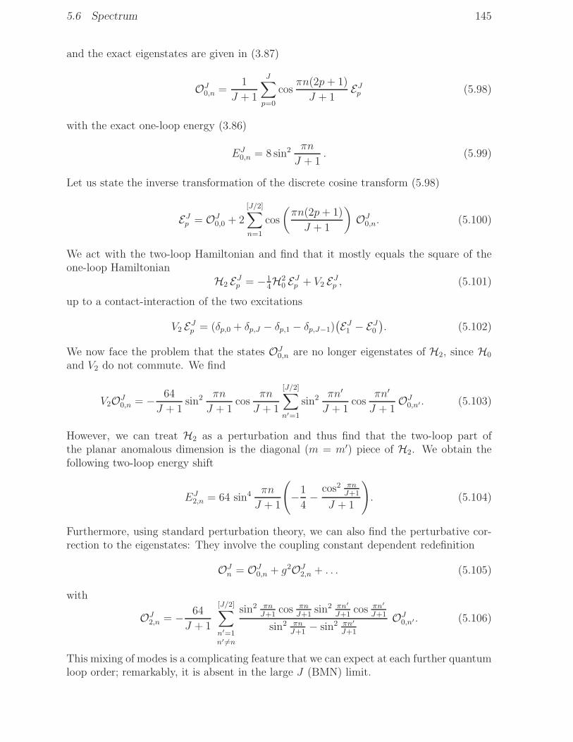
5.6 Spectrum 145
and the exact eigenstates are given in (3.87)
OJ0,n =1
J + 1
J∑
p=0
cosπn(2p+ 1)
J + 1EJp (5.98)
with the exact one-loop energy (3.86)
EJ0,n = 8 sin2 πn
J + 1. (5.99)
Let us state the inverse transformation of the discrete cosine transform (5.98)
EJp = OJ0,0 + 2
[J/2]∑
n=1
cos
(πn(2p+ 1)
J + 1
)OJ0,n. (5.100)
We act with the two-loop Hamiltonian and find that it mostly equals the square of theone-loop Hamiltonian
H2 EJp = −14H2
0 EJp + V2 EJp , (5.101)
up to a contact-interaction of the two excitations
V2 EJp = (δp,0 + δp,J − δp,1 − δp,J−1)(EJ1 − EJ0
). (5.102)
We now face the problem that the states OJ0,n are no longer eigenstates of H2, since H0
and V2 do not commute. We find
V2OJ0,n = − 64
J + 1sin2 πn
J + 1cos
πn
J + 1
[J/2]∑
n′=1
sin2 πn′
J + 1cos
πn′
J + 1OJ0,n′. (5.103)
However, we can treat H2 as a perturbation and thus find that the two-loop part ofthe planar anomalous dimension is the diagonal (m = m′) piece of H2. We obtain thefollowing two-loop energy shift
EJ2,n = 64 sin4 πn
J + 1
(
−1
4−
cos2 πnJ+1
J + 1
)
. (5.104)
Furthermore, using standard perturbation theory, we can also find the perturbative cor-rection to the eigenstates: They involve the coupling constant dependent redefinition
OJn = OJ0,n + g2OJ2,n + . . . (5.105)
with
OJ2,n = − 64
J + 1
[J/2]∑
n′=1n′ 6=n
sin2 πnJ+1
cos πnJ+1
sin2 πn′
J+1cos πn′
J+1
sin2 πnJ+1− sin2 πn′
J+1
OJ0,n′ . (5.106)
This mixing of modes is a complicating feature that we can expect at each further quantumloop order; remarkably, it is absent in the large J (BMN) limit.

146 5 Higher-Loops
We move on to three-loops and find that the result agrees with a general formula
DJn = D0 + g2E = J + 2 +
∞∑
ℓ=1
(8g2 sin2 πn
J + 1
)ℓ(cℓ +
ℓ−1∑
k,l=1
cℓ,k,lcos2l πn
J+1
(J + 1)k
)(5.107)
with the coefficients up to three-loops given by [38]
c1 = 1, c2 = −14, c2,1,1 = −1, c3 = 1
8, c3,k,l =
(+3
4+1
2
−34
+52
). (5.108)
As expected, the formula reproduces the energies of all states [0; 1; 0, J − 2] in Tab. 5.8.The coefficients cℓ agree with the prediction of string theory on plane-waves (3.99,3.98)
DJn = J + 2
√1 + λ′n2 +O(J−1), λ′ = 8π2g2/J2. (5.109)
This is a non-trivial result: Although we have only made use of the qualitative BMNlimit, the quantitative BMN energy formula seems to be the outcome.
We can also compare our result to string theory on a near plane-wave background[26,88]. This corresponds to an expansion of the results in powers of 1/J . Let us expandour result (5.107,5.108) to first order
DJn = J + 2 +
∞∑
ℓ=1
(λ′n2
)ℓ(cℓ + J−1
(−2ℓcℓ +
∑ℓ−1l=1cℓ,1,l
)+O(J−2)
)(5.110)
= J + 2 +(λ′n2
)(1− 2J−1
)+(λ′n2
)2(−14
+ 0J−1)
+(λ′n2
)3(18
+ 12J−1
)+ . . . .
This is to be compared to the near plane-wave string theory result [88] (the comparisontakes place at level 4 of the multiplet)
DJn = J + 2
√1 + λ′n2 − 2λ′n2 J−1 +O(J−2) (5.111)
= J + 2 +(λ′n2
)(1− 2J−1
)+(λ′n2
)2(−14
+ 0J−1)
+(λ′n2
)3(18
+ 0J−1)
+ . . . .
Structurally, both expression are equivalent and all coefficients agree except single oneat O(λ′ 3J−1). The same kind of disagreement was also observed for three excitations[129,102] and arbitrarily many of scalar type [130,131]. We will see further evidence of adisagreement between string theory and gauge theory starting at three loops in Sec. 6.5;we will discuss this issue there.
5.6.4 An Eighth-BPS state
Let us take a peek at non-planar physics within this sector: The lowest-dimensionaleighth-BPS state is expected to be a triple-trace state with weight w = (6; 0, 0; 0, 0, 4; 0, 6).Using the non-planar, one-loop Hamiltonian we find this protected state
O1/8−BPS = εabcεdef[N(N2 − 3) Trφaφd Trφbφe Trφcφf
+ 6(N2 − 1) Trφaφd Trφbφcφeφf − 12N Trφaφbφcφdφeφf
+ 8N Trφaφdφbφeφcφf + 4 Trφaφbφc Trφdφeφf]. (5.112)

5.6 Spectrum 147
It is annihilated by the operators
εabc[φb, φc], εabcε
αβ Trψα[φa, [φb, [φc, ψβ]]], (5.113)
which are part of the non-planar generalisations of S1,H0 and H1. This implies that thestate is protected (at least at one-loop).
It would be interesting to generalise some of the results of this chapter to includenon-planar corrections. At two-loops this might indeed be feasible as there are only fewnon-planar graphs.

148

149
Chapter 6
Higher-Loop Integrability
In this final chapter we would like to put together the results of the previous twochapters. In Ch. 5 we have seen how to make use of the interacting algebra to find higher-loop corrections. In Ch. 4 we have investigated the integrability of planar N = 4 SYM atthe one-loop level and demonstrated its usefulness. An obvious question is whether theintegrable structures persist even at higher-loops. This will be the subject of the currentchapter.
To start off, we shall introduce higher-loop integrability and argue that N = 4 gaugetheory (or, more precisely, the subsector discussed in Ch. 5) is indeed integrable at higher-loops. The main part of the chapter is devoted to the investigation of an integrable modelin the su(2) subsector. By making some assumptions on the form of interactions, we willfind that this model is uniquely determined at five-loops and, excitingly, reproduces theplane wave energy formula. What is more, we find the corresponding Bethe ansatz tocompute the spectrum at an arbitrary order in perturbation theory!
6.1 Higher-Loop Spin Chains
First of all, we would like to describe the notion of integrability for spin chains athigher-loops. We then go on by explaining why we believe that these structures shouldapply to higher-loop N = 4 SYM. Finally we will investigate the scaling behaviour ofcharges in the thermodynamic limit and describe how they can be defined canonically.
6.1.1 Aspects of Higher-Loop Integrability
To describe higher-loop corrections to scaling dimensions we have promoted the Hamil-tonian H = H0 of Ch. 3 to a function of the coupling constant H(g) in Ch. 5. At zerocoupling one recovers the one-loop Hamiltonian H(0) = H0. For higher-loop integrabilitywe do the same and promote the charges Qr = Qr,0 to functions Qr(g) with Qr(0) = Qr,0.A Hamiltonian H(g) = Q2(g) is considered to be higher-loop integrable if there existconserved charges Qr(g) with
‘higher-loop integrability ’: [Qr(g),Qs(g)] = [J(g),Qr(g)] = 0. (6.1)
In the case of N = 4 SYM, the symmetry algebra is psu(2, 2|4)×u(1). The u(1) factorcorresponds to the anomalous piece of the dilatation operator δD(g) which is conserved

150 6 Higher-Loop Integrability
in two-point functions. We will argue that N = 4 SYM in the planar limit might beintegrable for arbitrary values of the coupling constant g. The higher charges Qr(g) forman abelian algebra which enlarges the symmetry in the planar limit
psu(2, 2|4)× u(1) −→ psu(2, 2|4)× u(1)∞. (6.2)
Here, the u(1) anomalous dimension is absorbed into the set of integrable charges by theidentification δD(g) = g2H(g) = g2Q2(g).
An obstacle to the investigation of higher-loop integrability is that it apparently can-not be described with the formalism introduced in Sec. 4.1. The reason is that higher-loopinteractions are between several nearby fields, whereas an ordinary integrable spin chaininvolves nearest-neighbour interactions only.1 What is more, higher-loop interactions canchange the length of the spin chain giving rise to completely new structures. In order toconstruct a higher-loop integrable spin chain, the R-matrix of Sec. 4.1 appears to be notsuitable. For instance, it describes the scattering of two elementary spins and it is notyet understood how to generalise it to the interactions that occur at higher-loops. Con-sequently, we cannot even attempt to prove the associated Yang-Baxter equation, whichwould make higher-loop integrability manifest. Finally, there is not yet a constructivemeans to obtain higher charges.
In Sec. 4.1.3 we have shown how to extract the charges Qr,0 from the transfer matrixT (u, 0). Here, we can take the opposite direction and package all charges into a transfermatrix
T (u, g) = exp i
∞∑
r=2
ur−1Qr(g), (6.3)
which should satisfy the equivalent of (4.11)
[J(g), T (u, g)] = [T (u, g), T (v, g)] = 0. (6.4)
An interpretation of the transfer matrix might be as follows: An ordinary spin chain can beconsidered to be a composite object assembled from individual fields/spins/particles. Thetransfer matrix is derived from scattering processes of the individual particles. At higher-loops it is not known how to make sense of parton scattering processes. Nevertheless, itmight still be useful to consider the transfer matrix as a Wilson loop around the compositeobject. The identification of particles with fields/spins, however, would be lost for tworeasons: Interactions take place between more than two fields and the number of fields isnot even preserved. Instead, the Bethe ansatz (c.f. Sec. 4.3) offers an alternative notionof particles: The composite object has some vacuum state and its excitations correspondto particles. The interactions of such excitation particles are pairwise (right-hand side ofthe Bethe equations) and can therefore be integrable. This picture may be generalised tohigher-loops without complications.
6.1.2 The Local Charges
We do not know how to obtain the higher charges Qr explicitly and are thereforeforced to construct them by hand such that they satisfy (6.1). We cannot expect this
1Although non-nearest neighbour interactions of several spins are included in the tower of higherchargesQr, these cannot be related to the higher orders of the Hamiltonian because the charges commuteamong themselves, whereas the Hk’s in general do not.

6.1 Higher-Loop Spin Chains 151
to be feasible for finite values of g and restrict ourselves to a perturbative treatment. Infact, we know (parts of) H(g) only up to order g4 (three-loops) and we may construct thecharges Qr(g) only up to the same order. The algebra need not be satisfied exactly, butonly up to terms of higher order in perturbation theory
[Qr(g),Qs(g)] = [J(g),Qr(g)] = O(g2ℓ). (6.5)
For all-loop integrability the remaining higher-order terms would have to be cancelledby higher-order corrections to the charges. We now expand the charges in powers of thecoupling constant g
Qr(g) =∞∑
k=0
gkQr,k. (6.6)
The integrability condition (6.1) translates to the statement of perturbative integrability
‘perturbative integrability ’:
l∑
k=0
[Qr,k,Qs,l−k] =
l∑
k=0
[Jk,Qr,l−k] = 0. (6.7)
One important consideration for the construction of charges is their representation asan interaction acting on the spin chain, see Sec. 2.6.2. In Sec. 4.1.3 we have learned thatthe local charges Qr,0 act on r adjacent spins. In other words, the charge Qr,0 has 2r legs,r incoming and r outgoing ones. Although the higher-loop form of interactions describedin Sec. 2.6.2 applies to quantities that appear in correlators, it seems natural to generaliseit to the charges. An order gk correction to a generator J involves k + 2 legs and weconclude that for each power of g we should have one leg. In total, a charge Qr,k shouldhave 2r + k legs
Qr,k ∼{A1...AEi
B1...BEo
}, with Ei + Eo = 2r + k. (6.8)
It is also natural to assume that the charges have a definite parity, the same as at leadingorder
pQr(g) p−1 = (−1)rQr(g). (6.9)
Finally, the charges preserve the classical dimension
[D0,Qr(g)] = 0 (6.10)
when we identify the second charge with the anomalous dimension δD(g) = g2Q2(g),because D(g) and Q2(g) commute with all charges and so does their difference.
Let us now comment on the role of the Hamiltonian H(g). On the one hand, it belongsto the symmetry algebra psu(2, 2|4) when combined with D0
D0 + g2H(g) = D0 + δD(g) = D(g) ∈ psu(2, 2|4). (6.11)
On the other hand, H(g) is also one of the integrable charges. As such it is a generatorof the abelian algebra u(1)∞ defined by (6.1)
H(g) = Q2(g) ∈ u(1)∞. (6.12)
This is somewhat different from the situation at one-loop where the symmetry algebra istaken strictly at g = 0. The one-loop anomalous dilatation generator is an independentobject and belongs only to the abelian algebra u(1)∞.

152 6 Higher-Loop Integrability
6.1.3 Parity Pairs
As we have seen in Sec. 4.1.4, the integrable structure gives rise to pairs of stateswith degenerate energies and opposite parities. We have proved integrability only at one-loop, but a closer look at Tab. 5.8 reveals that the degeneracy of all one-loop pairs (±)is preserved even at three-loops!2 This is so for the pairs of the su(2) sector (•) [38], forpairs at the unitarity bound (∗), but also, and most importantly, for pairs away fromthe unitarity bound (unmarked). As discussed at the end of Sec. 5.1.4 all states of sucha multiplet are superpositions of states of different lengths. This is interesting becauseit shows that also for truly dynamic spin chains with a fluctuating number of sites,integrability is an option.
We do not know how to use the R-matrix formalism beyond one-loop, if this is possibleat all. Therefore we cannot rigorously prove higher-loop integrability by means of aYang-Baxter equation. One might construct several of the higher charges explicitly athigher-loops and thus make integrability very plausible, but this would not constitutea proof. Instead, we shall be satisfied by demonstrating the preservation of degeneratepairs at three-loops. This is certainly a necessary condition for integrability, but at firstsight it appears not to imply the existence of commuting charges. Nevertheless, there aresome indications that pairing is indeed sufficient to guarantee integrability. First of all, asystematic pairing is most naturally explained by the following set of identities
[H(g),Q(g)] = [p,H(g)] = {p,Q(g)} = 0 (6.13)
among the Hamiltonian H(g), parity p and some charge Q(g). The investigations forthe model in Sec. 6.2 have shown that indeed we can construct a charge Q(g) = Q3(g)whenever the spectrum has sufficiently many pairs without imposing further constraints onthe Hamiltonian H(g). More remarkably, it always turned out to be possible to constructconserved charges Qr(g) as soon as the Hamiltonian pairs up states. The charges do notonly commute with the Hamiltonian, but also among themselves, i.e. they automaticallysatisfy (6.1). This parallels earlier observations [80] that it appears close to impossible toconstruct systems with [Q2,Q3] = 0 which do not have arbitrarily many other commutingcharges Qr, i.e. which are not integrable.
It is therefore likely that planar N = 4 SYM (at least) in the su(2|3) subsector and (atleast) at three-loops is integrable. In agreement with the findings of [79] we conclude thatintegrability appears to be a consequence of field theory combined with symmetry anddoes not depend on the specific model very much. It strongly supports the idea of all-loopintegrability in planar N = 4 SYM. What is more, the dynamic aspects of higher-loopspin chains appear to be no obstruction. Let us emphasise, though, that a rigorous proofof higher-loop integrability remains a challenge.
6.1.4 The su(2|3) Sector Revisited
At this point we can reinvestigate the undetermined coefficients of the su(2|3) spinchain at three-loops, c.f. Sec. 5.5. By imposing
[Q(g),H(g)] = [S(g),H(g)] = O(g6) (6.14)
2Let us emphasise that, even if the table was computed assuming BMN scaling to fix the values ofα1, α3, σ1, σ2, the pairing holds for generic values.

6.1 Higher-Loop Spin Chains 153
we found that H4 depends on four relevant coefficients σ1,2,3,4. The coefficients σ3,4 multi-ply invalid structures, whereas σ1 corresponds to a redefinition of the coupling constant.The remaining coefficient σ2 multiplies Q4,0 which is structurally equivalent to H4 andsatisfies [J(g),Q4(g)] = 0 as well. In fact, by imposing [Q(g), X(g)] = [S(g), X(g)] = 0we do not only find H(g), but also all the other even generators Qr(g) of the abelianalgebra of integrable charges u(1)∞. Thus σ2 corresponds to the transformation
H(g) 7→ H(g) + σ2 g4Q4(g), (6.15)
which has no influence on (6.14) due to [J(g),Qr(g)] = 0. This degree of freedom may befixed by considering the anticommutator of supercharges (5.9) at order g6
6∑
k=0
{(Sk)
αa, (Q6−k)
bβ
}= 1
2δbaδ
αβH4. (6.16)
Unfortunately, this equation involves Q6,S6 which are part of a four-loop calculationand out of reach here. We believe that (6.16) will force the coefficient σ2 to vanish,and in conclusion all corrections up to three loops would be determined uniquely (upto a redefinition of the coupling constant). At higher loops this picture is expected tocontinue: While [Q(g), X(g)] = [S(g), X(g)] = 0 determines the even elements Qr ofu(1)∞, the anticommutator {S(g),Q(g)} yields the one element Q2(g) = H(g) which isalso associated to su(2|3) as the generator D0 + 3
2g2H(g). It is reasonable to assume that
σ2 may alternatively be fixed by the non-planar algebra where conservation of the chargeQ4 is lost.
Let us comment on the effect of integrability on the degrees of freedom for similar-ity transformations. Similarity transformations are symmetries of the algebra relationsand thus give rise to undetermined coefficients in the construction of the most generaldeformation of generators. In Sec. 5.5 we argued that the coefficients which arise forthe generators Jk are in one-to-one correspondence with the structures that can be usedfor the construction of Hk−2, see also Tab. 5.4. However there are also some similaritytransformations which do not change the generators. These are generated by invariantoperators such as H(g) and, to some extent, the length L. In an integrable system thereare more invariant operators: The charges Qr(g). Only the even charges Qr are compati-ble with the structure of Hk−2. For example, the fourth charge will appear as a symmetryin Tab. 5.4 starting at sixth order (four-loops).
6.1.5 The Thermodynamic Limit
The thermodynamic limit is the limit in which the length of the spin chain L as wellas the number of excitations is taken to infinity while focusing on the the low-energyspectrum, c.f. Sec. 4.5. In this limit it was observed that the r-th charge Qr,0 at one-loopscales as L1−r [68]. Here, we would like to generalise the thermodynamic limit to higher-loops. From the investigation of the closely related BMN limit (c.f. Sec. 3.6) as well asfrom classical spinning strings (c.f. Sec. 4.6), we infer that each power of the couplingconstant g should be accompanied by one power of 1/L. It is common belief that thisscaling behaviour holds for perturbative gauge theory, but it is clearly not a firm fact.We shall assume its validity for several reasons: Firstly, it was not only confirmed at

154 6 Higher-Loop Integrability
one-loop, but also at two-loops [25, 38]. It is a nice structure and conceptually it wouldbe somewhat disappointing if broken at some higher loop order. Secondly, the AdS/CFTcorrespondence seems to suggest it. Thirdly, it will allow us to define charges uniquely,see below, and arrive at a unique result in Sec. 6.2.
In conclusion, the scaling of charges in the thermodynamic limit is given by3
Qr,k = limL→∞
Lk+r−1Qr,k, T (u, g) = limL→∞
T (Lu, Lg). (6.17)
6.1.6 Canonical Charges
As the charges form an abelian algebra, one can replace Qr(g) by some polynomialQ′r(g) in the charges without changing the algebra. We will now prove the uniqueness of
the ‘canonical’ set of charges with good structural (c.f. Sec. 6.1.2) and scaling properties(c.f. Sec. 6.1.5). We will start by assuming that the charges Qr(g) are canonical and showthat we cannot change them without spoiling the one of the properties.
The charges can be written as a local interaction Qr,k =∑L
p=1Qr,k,p... with the localcharge density Qr,k,p.... A generic polynomial transformation would therefore make Q′
r
multi-local in general. To preserve locality we are restricted to linear transformationswhich are generated by
Q′r(g) = Qr(g) + αr,s,l g
2lQr+2s(g). (6.18)
We now find two constraints on l and s: On the one hand, there is the structuralconstraint (6.8) which tells that Q′
r,k can only have 2r + k legs. This requires
l ≥ 2s. (6.19)
On the other hand, a correct scaling in the thermodynamic limit (6.17) requires that Q′r,k
scales as O(L1−k−r). In order not to spoil scaling, we need
l ≤ s. (6.20)
Together, these two constraints imply l ≤ 0, but we do not allow negative powers of g.In total we get l = s = 0 or, in other words, Qr can only be rescaled by a constant αr,0,0.Finally, this constant can be fixed by using the canonical transfer matrix T (u, 0) of theone-loop spin-chain, c.f. Sec. 4.1.3.
In conclusion, the canonical definition for Qr(g) is unique (if it exists). As H(g) issubject to the same constraints as Q2(g), both of them must be equal H(g) = Q2(g).
6.2 The su(2) Sector at Higher-Loops
In this section we will construct a model for higher-loop anomalous dimensions inthe su(2) subsector of N = 4 SYM. We will rely on three assumptions on the formof interactions: (i) Integrability, (ii) the thermodynamic limit and (iii) some constraintsinspired by Feynman diagrammatics. Note that none of these assumptions should be taken
3In the BMN we would account for the finite number of excitations by the slightly modified definitionsQr,k = Lk+rQr,k and T (u, g) = T (Lu, Lg)L

6.2 The su(2) Sector at Higher-Loops 155
as a firm fact. Whether or not they are fully justified in (perturbative) N = 4 SYM willnot be the subject of this chapter, but we believe that the model shares several featureswith higher-loop gauge theory and therefore deserves an investigation. Intriguingly, itwill turn out to be unique up to (at least) five-loops and agree with the excitation energyformula in the BMN limit! At any rate, this makes it a very interesting model to considerin its own right. With some luck, the assumptions (i-iii) will turn out to be valid forN = 4 SYM and we have constructed the planar, five-loop4 dilatation generator in thesu(2) subsector.
6.2.1 Interactions
In the su(2) sector, the number of field sites is conserved. In particular, this impliesthat odd powers of g are not allowed. Furthermore, rotations are manifestly realised, thesu(2) generators do not receive radiative corrections. Therefore the interactions can onlybe of the form (see Sec. 2.6.2) { a1 . . . aE
aπ(1) . . . aπ(E)
}(6.21)
with π some permutation of E elements.5 Any permutation can be represented in termsof elementary permutations Pp,p+1 of adjacent fields. A generic term will be written as
{p1, p2, . . .} =L∑
p=1
Pp+p1,p+p1+1Pp+p2,p+p2+1 . . . . (6.22)
For example, in this notation the one-loop dilatation generator (3.75) is given by
H0 = Q2,0 =({} − {1}
). (6.23)
This notation is useful due to the nature of maximal scalar diagrams as discussed at theend of Sec. 2.5.3: An interaction of scalars at ℓ loops with the maximal number of 2 + 2ℓlegs can be composed from ℓ crossings of scalar lines. In the planar limit, the crossingscorrespond to elementary permutations and at ℓ-loops there should be no more than ℓpermutations. In field theory this is a feature of maximal diagrams, but here we willassume the pattern to hold in general. Furthermore, in Sec. 4.1.3 we have learned thatthe r-th charge at leading (one-loop) order can be constructed from r − 1 copies of theHamiltonian density which, in this case (6.23), is essentially an elementary permutation.We will therefore assume the contributions to the charges to be of the form
Qr,2ℓ−2 ∼ {p1, . . . , pm} with m ≤ r + ℓ− 2 and 1 ≤ pi ≤ r + ℓ− 2. (6.24)
Finally, the even (odd) charges should be parity even (odd) and (anti)symmetric.6
Parity acts on the interactions as
p {p1, . . . , pm} p−1 = {−p1, . . . ,−pm}, (6.25)
4We disregard wrapping interactions, see Sec. 2.6.3, i.e. this applies only to states of length L ≥ 6.5Note that we will consider the states to be sufficiently long and drop wrapping interactions
(c.f. Sec. 2.6.3). We will comment on the role of wrappings in Sec. 6.5.4.6In fact, the Hamiltonian H(g) and charges Qr(g) should be hermitian. The coefficients of the in-
teraction structures should therefore be real (imaginary) for even (odd) r. Reality of the Hamiltonianfollows from the equivalence of the Hamiltonian for the su(2) sector and its conjugate.

156 6 Higher-Loop Integrability
whereas symmetry acts as
{p1, . . . , pm}T = {pm, . . . , p1}. (6.26)
Symmetry will ensure that the eigenvalues of the charges are real.Note that the interaction symbols are subject to several identities which can be used
to bring them into some normal form. One identity involves a repeated elementary per-mutation
{. . . , p, p, . . .} = {. . . , . . .}. (6.27)
Another obvious identity
{. . . , p, p′, . . .} = {. . . , p′, p . . .} if |p− p′| ≥ 2 (6.28)
allows to commute two non-overlapping elementary permutations. A third identity is dueto gauge invariance or cyclic invariance of interactions
{p1 + p′, . . . , pm + p′} = {p1, . . . , pm}. (6.29)
Finally, the spin at each site can take two different values and we cannot antisymmetrisemore than two spins. This leads to the the identity
{. . . , p, p± 1, p, . . .} = {. . . , . . .} − {. . . , p, . . .} − {. . . , p± 1, . . .}+ {. . . , p, p± 1, . . .}+ {. . . , p± 1, p, . . .}. (6.30)
6.2.2 The Higher Charges
We would now like to construct some of the higher charges for the model in Ch. 5explicitly. Let us start by writing down the Hamiltonian in Tab. 5.2,5.6, restricted to thesu(2) subsector in the notation introduced above
H0 = {} − {1},H2 = (−2 + 2α3){}+ (3− 2α3){1} − 1
2
({1, 2}+ {2, 1}
),
H4 =(
152− 8α3 + σ1 − 2
3σ2
){}+
(−13 + 12α3 − σ1 + 4
3σ2
){1}+ 1
2{1, 3}
+(3− 2α3 − 1
3σ2
)({1, 2}+ {2, 1}
)+(−1
2+ 1
3σ2
)({1, 2, 3}+ {3, 2, 1}
)
+(−1
3σ2 − iξ3
){2, 1, 3}+
(−1
3σ2 + iξ3
){1, 3, 2}. (6.31)
Here, we should set σ1 = σ2 = α3 = 0 to obtain the correct scaling behaviour in the ther-modynamic limit, see Sec. 5.6.1. Furthermore, the coefficient ξ3 is related to a similaritytransformation; it consequently does not affect scaling dimensions and we set it to zero.7
According to Sec. 4.1.3, the leading order third charge is given by
Q3,0 = i2
({1, 2} − {2, 1}
). (6.32)
As discussed in Sec. 6.1.4, the leading fourth charge can be read off from H4 as thestructure multiplied by σ2
Q4,0 = −23{}+ 4
3{1} − 1
3({1, 2}+ {2, 1})
− 13
({1, 3, 2}+ {2, 1, 3}
)+ 1
3
({1, 2, 3}+ {3, 2, 1}
). (6.33)
7Furthermore, the coefficients of interaction structures can be assumed to be real for the Hamiltonian.

6.2 The su(2) Sector at Higher-Loops 157
Both of them commute with H0 and among themselves.Let us now go ahead and compute the first correction to a higher charge. For Q3,2 the
only suitable structures are ({1, 2} − {2, 1}) and ({1, 2, 3} − {3, 2, 1}). We demand thatQ3(g) commutes with H(g) in perturbation theory
[H0,Q3,2] + [H2,Q3,0] = 0 (6.34)
and find the coefficient of ({1, 2, 3} − {3, 2, 1}) to be fixed to i/2. The coefficient of({1, 2} − {2, 1}) cannot be determined because this structure is proportional to Q3,0 andcommutes with H0 by construction. We can only fix it by demanding a correct scalingbehaviour in the thermodynamic limit, c.f. Sec. 6.1.5,6.1.6 and obtain
Q3,2 = −2i({1, 2} − {2, 1}
)+ i
2
({1, 2, 3} − {3, 2, 1}
). (6.35)
We proceed in the same way to determine the integrable charges Q3,Q4 up to O(g4)(three-loops). The unique solution with correct scaling in the thermodynamic limit ispresented in Tab. 6.2.
6.2.3 Higher-Loop Construction
Here we would like to construct the most general (i) integrable higher-loop spin chainwith (ii) the proposed scaling in the thermodynamic limit. For that purpose, we make themost general ansatz for the charges in terms of (iii) permutation symbols {. . .} multipliedby undetermined coefficients. We then demand that the charges mutually commute andhave the right scaling behaviour in the thermodynamic limit. We will use the computeralgebra system Mathematica to preform all necessary commutators and solve the arisingsets of linear equations to determine the coefficients. Some of the methods used in theconstruction are given in App. E. Let us describe the details of our construction of theintegrable model:8
• We make the ansatz that the charges Qr,2ℓ−2 with r even (odd), have even (odd)parity and are (anti)symmetric. They consist of no more than r + ℓ − 2 elementarypermutations ranging over r + ℓ− 1 adjacent sites, see Sec. 6.2.1.
• We compute the commutator of H and Q3 (up to five-loops). By demanding that itshould vanish, we obtain a set of linear equations among the coefficients. We solve itfor coefficients of Q3 as far as possible, but some equations relate coefficients of Q2
only among themselves.
• Alternatively, we may ignore the charge Q3 and only demand that all pairs in the spec-trum of H remain degenerate at higher-loops. This yields the same set of constraintsfor the coefficients of H (up to four-loops).
• We then compute the commutator of H and Qr (for r = 3, 4 up to ℓ = 4 and forr = 5, 6 up to ℓ = 2). This constrains most coefficients of Qr and remarkably yieldsno new constraints for H.
8We keep track of the number of free coefficients in Tab. 6.4. We shall also indicate in the text atwhat loop order ℓ the individual calculations have been performed.

158 6 Higher-Loop Integrability
H0 = +{} − {1},H2 = −2{}+ 3{1} − 1
2
({1, 2}+ {2, 1}
),
H4 = +152{} − 13{1}+ 1
2{1, 3}+ 3({1, 2}+ {2, 1})− 1
2
({1, 2, 3}+ {3, 2, 1}
),
Q3,0 = + i2
({1, 2} − {2, 1}
),
Q3,2 = −2i({1, 2} − {2, 1}
)+ i
2
({1, 2, 3} − {3, 2, 1}
),
Q3,4 = +73i8
({1, 2} − {2, 1}
)− i
4
({1, 2, 4}+ {1, 3, 4} − {1, 4, 3} − {2, 1, 4}
)
− 7i2
({1, 2, 3} − {3, 2, 1}
)− i
8
({1, 3, 2, 4} − {2, 1, 4, 3}
)
− i8
({1, 2, 4, 3} − {1, 4, 3, 2}+ {2, 1, 3, 4} − {3, 2, 1, 4}
)
+ 5i8
({1, 2, 3, 4} − {4, 3, 2, 1}
),
Q4,0 = −23{}+ 4
3{1} − 1
3({1, 2}+ {2, 1})
− 13
({1, 3, 2}+ {2, 1, 3}
)+ 1
3
({1, 2, 3}+ {3, 2, 1}
),
Q4,2 = +5{} − 313{1}+ 2
3{1, 3}+ 17
6
({1, 2}+ {2, 1}
)+ 11
6
({1, 3, 2}+ {2, 1, 3}
)
− 136
({1, 2, 3}+ {3, 2, 1}
)− 1
3{2, 1, 3, 2} − 1
6
({1, 3, 2, 4}+ {2, 1, 4, 3}
)
− 16
({1, 2, 4, 3}+ {1, 4, 3, 2}+ {2, 1, 3, 4}+ {3, 2, 1, 4}
)
+ 12
({1, 2, 3, 4}+ {4, 3, 2, 1}
),
Q4,4 = −632{}+ 401
6{1} − 20
3{1, 3} − 5
6{1, 4} − 77
4
({1, 2}+ {2, 1}
)
− 616
({1, 3, 2}+ {2, 1, 3}
)+ 1
2
({1, 2, 4}+ {1, 3, 4}+ {1, 4, 3}+ {2, 1, 4}
)
+ 836
({1, 2, 3}+ {3, 2, 1}
)+ 8
3{2, 1, 3, 2} − 1
6
({1, 2, 4, 5}+ {2, 1, 5, 4}
)
+ 16
({1, 3, 2, 5}+ {1, 3, 5, 4}+ {1, 4, 3, 5}+ {2, 1, 3, 5}
)
+ 1912
({1, 3, 2, 4}+ {2, 1, 4, 3}
)+ 1
6
({1, 2, 5, 4}+ {2, 1, 4, 5}
)
+ 1712
({1, 2, 4, 3}+ {1, 4, 3, 2}+ {2, 1, 3, 4}+ {3, 2, 1, 4}
)
− 16
({1, 2, 3, 5}+ {1, 3, 4, 5}+ {1, 5, 4, 3}+ {3, 2, 1, 5}
)
− 194
({1, 2, 3, 4}+ {4, 3, 2, 1}
)+ 1
12
({1, 4, 3, 2, 5}+ {2, 1, 3, 5, 4}
)
+ 112
({1, 3, 2, 5, 4}+ {2, 1, 4, 3, 5}
)+ 1
12
({1, 2, 5, 4, 3}+ {3, 2, 1, 4, 5}
)
− 16
({1, 3, 2, 4, 3}+ {2, 1, 3, 2, 4}+ {2, 1, 4, 3, 2}+ {3, 2, 1, 4, 3}
)
− 14
({1, 2, 4, 3, 5}+ {1, 3, 2, 4, 5}+ {2, 1, 5, 4, 3}+ {3, 2, 1, 5, 4}
)
− 14
({1, 2, 3, 5, 4}+ {1, 5, 4, 3, 2}+ {2, 1, 3, 4, 5}+ {4, 3, 2, 1, 5}
)
+ 34
({1, 2, 3, 4, 5}+ {5, 4, 3, 2, 1}
).
Table 6.2: The Hamiltonian H = Q2 and the charges Q3,Q4 at three-loops.

6.2 The su(2) Sector at Higher-Loops 159
ℓ 1 2 3 4 5structures for H2ℓ−2 2 3 6 12 27integrability 0 0 2 5 17integrable H2ℓ−2 2 3 4 7 10structures for T2ℓ−2 0 0 0 1 3H2ℓ−2 relevant 2 3 4 6 7propagation 1 2 3 4 5two-spin interaction 0 0 1 2 2(+1)remaining d.o.f. 1 1 0 0 0
ℓ 1 2 3 4 5structures for Q3,2ℓ−2 1 2 6 15 46integrability 0 1 4 13 43Q3,2ℓ−2 1 1 2 2 3
structures for Q4,2ℓ−2 6 12 27 63integrability 3 9 23 59Q4,2ℓ−2 3 3 4 4
Table 6.4: Number of coefficients for the higher-loop integrable su(2) spin chain
• All the obtained charges Qr commute among themselves without further constraints.We notice that the remaining degrees of freedom correspond precisely to linear re-definitions of charges, c.f. the right hand side of Tab. 6.4: We can rescale the chargeQ3 by a function of the coupling constant, this yields one degree of freedom at eachloop order. We may also add g4f(g2)Q5(g) which is structurally equivalent to Q3(g),this yields one degree of freedom starting from ℓ = 3. For Q4 the story is equivalent.Here, we can always add the length operator L as well as the the Hamiltonian H orrescale by a function. This gives three degrees of freedom for all loop orders. Startingfrom ℓ = 3 there are further degrees of freedom due to Q6. All in all, this is just theexpected number of coefficients. In the thermodynamic limit (should it exist at all),all coefficients would be fixed for the canonical charges, see Sec. 6.1.6.
In this way we have established the most general integrable system for the assumed setof interactions. We conclude that, indeed, the pairing of states appears to be a sufficientcondition for integrability (in this model). Next we would like to impose the thermody-namic limit. For the thermodynamic limit we make use of two processes: Propagationof a single excitation and interaction of two excitations. These should yield the correctscaling behaviour at each loop order.
• In Sec. 3.6 we have seen that the planar one-loop dilatation operator acts on theposition of a single excitation as a lattice Laplacian �. The resulting eigenstates areFourier modes. The lowest, non-zero eigenvalue of the Laplacian is proportional to1/L2, exactly the right behaviour for H0. Due to the form of the interaction, H2ℓ−2
must act as a polynomial in � of degree ℓ. For the correct scaling behaviour, 1/L2ℓ,all terms �
k with k < ℓ should be absent. In general, this determines ℓ coefficients,see Tab. 6.4. We shall not fix the coefficient of �
ℓ although the quantitative BMNexcitation energy formula H(g) = (
√1− 2g2�− 1)/g2 predicts it
H2ℓ−2 ∼ −2−ℓ−1Cℓ−1�ℓ (6.36)
with Ck = (2k)!/k!(k+1)! the Catalan numbers governing the expansion of the squareroot.
• The interaction of two excitations is a more delicate issue, it is obtained by actingwith H2ℓ−2 on two excitations and subtracting the contribution from the propagationof the individual excitations. The remainder can only be non-zero if both excitations

160 6 Higher-Loop Integrability
are close (the distance depends on the loop order), in other words the remainder isa contact interaction. This interaction must also be suppressed by sufficiently highpowers of 1/L.
Let us investigate the first order effect of the contact term for states with only twoexcitations, see Sec. 5.6.3. The first order is determined by diagonal scattering, wetherefore compute the matrix element of O0,n going into itself. First of all, this is sup-pressed by 1/L due to phase space considerations. Furthermore, there is a suppressionof n2n′ 2/L4 for the process O0,n → O0,n′. This is due to the zero mode state O0,0 whichmust be annihilated and can never be produced. In total there is a suppression of 1/L5
for the contact term, this is sufficient for ℓ = 2. Starting from three-loops, the contactterm may violate the scaling behaviour and there will be additional constraints. Atthree-loops a single constraint is enough to remove terms of order 1/L5. At four-loopswe need to remove terms of orders 1/L5 and 1/L7 yielding two constraints. At ℓ = 5there are three constraints, but only two independent coefficients which may influencethe scaling behaviour. Miraculously, the three constraints seem to be degenerate suchthat the scaling in the thermodynamic limit appears to be fine at five-loops.
To impose the constraints is not a trivial task.9 The problem is that also iteratedcontact terms of perturbation theory may violate the scaling in the thermodynamiclimit. These must be cancelled by higher order contact terms. We will thereforeconsider only states with exactly two excitations for which closed expression can befound. We will assume that the conjectured energy formula (5.107) holds to all orders.We will then compute the energies of several two-excitation states at higher-loops andmatch them with the formula. This can only be possible if a qualitative BMN limitexists and the coefficients are adjusted such that Hamiltonian provides the correctscaling.
• At this point nearly all relevant coefficients are fixed. However, starting at four-loops, there are some free coefficients left which have no influence on the scalingdimensions. These are due to the freedom to rotate the space of states with anorthogonal transformation generated by an antisymmetric operator A. For the four-loop interactions there is precisely one antisymmetric operator A6, it happens to beproportional to [Q2,0,Q2,2]. It gives rise to the following similarity transformation
Qr(g) 7→ exp(αg6A6)Qr(g) exp(−αg6A6). (6.37)
The leading term in H = Q2 due to the transformation is
H6 7→ H6 + α[A6,H0]. (6.38)
Consequently, the eigenvalues of H(g) are not changed and α only affects the eigen-vectors. Similarly, at five-loops there are three even antisymmetric operators for theconstruction of A8.
There are some interesting points to be mentioned regarding this solution. First of all,integrability and the thermodynamic limit fix exactly the right number of coefficients for
9It would be interesting to find a general criterion which determines whether an interaction of two ormore excitations has the correct scaling or not.

6.3 Spectrum 161
a unique solution. For this solution, the contribution δE of one excitation to the energyin the BMN limit is given by (recall that g2 = g2/J2 = λ′/8π2 and D = D0 + g2E)
δEn =c1g2
(√1 + c2 8π2n2g2 − 1
)+O(g10) (6.39)
The constants c1, c2 correspond to symmetries of the equations, they can therefore notbe fixed by algebraic arguments. We will set them to their physical values, c1 = c2 = 1.It is interesting to observe that the BMN quantitative square-root formula for the energyof one excitation is predicted correctly; we have only demanded that the thermodynamic(i.e. qualitative BMN limit) limit exists. Finally, let us mention that the three-loopcontribution agrees precisely with the calculation of Ch. 5. For the physical choice ofc1, c2 we present the four-loop and five-loop contribution to the Hamiltonian in Tab. 6.6.
6.3 Spectrum
We can now apply the higher-loop integrable Hamiltonian to obtain some energies. Inaddition we can evaluate the integrable charges on the eigenstates of the Hamiltonian.
6.3.1 Lowest-Lying States
In preparation for the next section, it will be helpful to know the spectrum of lowest-lying modes for our spin chain. To obtain a matrix representation for the operators,we have used standard higher order quantum mechanical perturbation theory. We haveapplied the Hamiltonian H and charges Q3,Q4 up to four-loops to all states with agiven length L and number of excitations K. The computations were performed usingthe routines in App. E. Then, the leading order energy matrix was diagonalised toobtain the leading order energy eigenvalues. Next, the off-diagonal terms at higher-loopswere removed iteratively by a sequence of similarity transformations, see also Sec. 5.6.2.Afterwards, the Hamiltonian is diagonal and we can read off the energy eigenvalues. Thesame similarity transformations which were used to make H diagonal also diagonaliseQ3,Q4 and we may read off their eigenvalues.
We present our findings up to L = 8 in Tab. 6.8 (we omit the protected states withK = 0) which is read as follows: For each state there is a polynomial and we write downthe coefficients up to O(g8) and O(x2). For single states the polynomial X(x, g) equalssimply
X(x, g) = E(g) + x2Q4(g). (6.40)
If there is more than one state transforming in the same representation, the eigenvaluesare solutions to algebraic equations. These could be solved numerically, here we prefer tostate the exact algebraic equation in terms of a polynomial X(ω, x, g) of degree k − 1 inω (k is also the number of lines in one block, one for each coefficient of the polynomial).The energy and charge eigenvalues are determined through the formula
ω = E(g) + xQ3(g) + x2Q4(g), ωk = X(ω, x, g). (6.41)
At first sight the terms linear in x may appear spurious and the corresponding chargeQ3(g) would have to be zero. For unpaired states with non-degenerate Q2(g) this is true,

162 6 Higher-Loop Integrability
H6 = −35{}+(67 + 4α
){1}+
(−21
4− 2α
){1, 3} − 1
4{1, 4}
+(−151
8− 4α
)({1, 2}+ {2, 1}
)+ 2α
({1, 3, 2}+ {2, 1, 3}
)
+ 14
({1, 2, 4}+ {1, 3, 4}+ {1, 4, 3}+ {2, 1, 4}
)+(6 + 2α
)({1, 2, 3}+ {3, 2, 1}
)
+(−3
4− 2α
){2, 1, 3, 2}+
(98
+ 2α)({1, 3, 2, 4}+ {2, 1, 4, 3}
)
+(−1
2− α
)({1, 2, 4, 3}+ {1, 4, 3, 2}+ {2, 1, 3, 4}+ {3, 2, 1, 4}
)
− 58
({1, 2, 3, 4}+ {4, 3, 2, 1}
),
H8 = +14798{}+
(−1043
4− 12α+ 4β1
){1}+
(−19 + 8α− 2β1 − 4β2
){1, 3}
+(5 + 2α + 4β2 + 4β3
){1, 4}+ 1
8{1, 5}+
(11α− 4β1 + 2β3
)({1, 2}+ {2, 1}
)
− 14{1, 3, 5}+
(2514− 5α + 2β1 − 2β3
)({1, 3, 2}+ {2, 1, 3}
)
+(−3− α− 2β3
)({1, 2, 4}+ {1, 3, 4}+ {1, 4, 3}+ {2, 1, 4}
)
− 18
({1, 2, 5}+ {1, 4, 5}+ {1, 5, 4}+ {2, 1, 5}
)
+(
414− 6α + 2β1 − 4β3
)({1, 2, 3}+ {3, 2, 1}
)+(−107
2+ 4α− 2β1
){2, 1, 3, 2}
+(
14
+ β2
)({1, 3, 2, 5}+ {1, 3, 5, 4}+ {1, 4, 3, 5}+ {2, 1, 3, 5}
)
+(
1834− 6α+ 2β1 − 2β2
)({1, 3, 2, 4}+ {2, 1, 4, 3}
)
+(−3
4− 2β2
)({1, 2, 5, 4}+ {2, 1, 4, 5}
)+(1 + 2β2
)({1, 2, 4, 5}+ {2, 1, 5, 4}
)
+(−51
2+ 5
2α− β1 + β2 + 3β3
)({1, 2, 4, 3}+ {1, 4, 3, 2}+ {2, 1, 3, 4}+ {3, 2, 1, 4}
)
− β2
({1, 2, 3, 5}+ {1, 3, 4, 5}+ {1, 5, 4, 3}+ {3, 2, 1, 5}
)
+(
354
+ α + 2β3
)({1, 2, 3, 4}+ {4, 3, 2, 1}
)
+(−7
8− α+ 2β3
)({1, 4, 3, 2, 5}+ {2, 1, 3, 5, 4}
)
+(
12
+ α)({1, 3, 2, 5, 4}+ {2, 1, 4, 3, 5}
)
+(
58
+ 12α− β3
)({1, 3, 2, 4, 3}+ {2, 1, 3, 2, 4}+ {2, 1, 4, 3, 2}+ {3, 2, 1, 4, 3}
)
+(
14− 2β3
)({1, 2, 5, 4, 3}+ {3, 2, 1, 4, 5}
)
+(
14
+ 12α + β3
)({1, 2, 4, 3, 5}+ {1, 3, 2, 4, 5}+ {2, 1, 5, 4, 3}+ {3, 2, 1, 5, 4}
)
+(−1
2α− β3
)({1, 2, 3, 5, 4}+ {1, 5, 4, 3, 2}+ {2, 1, 3, 4, 5}+ {4, 3, 2, 1, 5}
)
− 78
({1, 2, 3, 4, 5}+ {5, 4, 3, 2, 1}
)
Table 6.6: Four-loop and five-loop contributions to the Hamiltonian.

6.3 Spectrum 163
L K P g0x0 g2x0 g4x0 g6x0 g0x2 g2x2 g4x2 g6x2
4 2 + +6 −12 +42 ∗ +0 ∗ ∗ ∗5 2 − +4 −6 +17 −115
2+8
3−8 ∗ ∗
6 2 + +10ω −17ω +1172ω −1037
4ω −10
3ω +30ω −381
2ω ∗
−20 +60 −230 +1025 +0 −1403
+420 ∗6 3 − +6 −9 +63
2−621
4−6 +36 +0 ∗
7 2 − +2 −32
+3716
−28364
+43
−52
+8116
−70764
7 2 − +6 −212
+55516
−899764
+0 +92
−51316
+1190764
7 3 ± +10ω −15ω +50ω −8754ω −10
3ω +25ω −285
2ω +1615
2ω
−25 +75 −12254
+58754
+24512
−180 +2814524
−8687512
8 2 + +14ω2 −23ω2 +79ω2 −349ω2 −143ω2 +39ω2 −250ω2 +4691
3ω2
−56ω +172ω −695ω +3254ω +563ω −700
3ω +5258
3ω −11822ω
+56 −224 +966 −4585 −0 +168 −50543
+382693
8 3 − +6 −9 +33 −162 −6 +33 −192 +1191
8 3 ± +8ω −10ω +28ω −102ω +43ω −2ω +4ω −26
3ω
−16 +40 −137 +548 −43
−403
+3283
−19483
8 4 + +20ω2 −32ω2 +112ω2 −511ω2 −323ω2 +72ω2 −442ω2 +8264
3ω2
−116ω +340ω −1400ω +6938ω +3923ω −3100
3ω +20708
3ω −45348ω
+200 −800 +3600 −18400 −320 +2800 −584003
+3896803
Table 6.8: Four-loop energies and charges Q3,4. See Sec. 6.3.1 for an explanation.
but not so for pairs of degenerate states. Then the solution of the algebraic equation leadsto terms of the sort
√0 + x2 = ±x, where the 0 is meant to represent the degeneracy.
Note that for some states the interaction is longer than the state. In such a case, indicatedby ∗ in the table, we do not know the energy/charge eigenvalue, see also Sec. 6.5.4.
6.3.2 Two Excitations
Now that the Hamiltonian is known up to five loops, we may continue the analysis ofthe two-excitation states in Sec. 5.6.3. In principle, we should diagonalise the energy inperturbation theory, however, this is very labourious. Instead we will assume the all-loopformula (5.107) to be correct and match the coefficients to sufficiently many two-excitationstates.10 When the coefficients have been determined, we may compare the formula tofurther states and find agreement. We take this as compelling evidence that the obtainedformula and coefficients are indeed correct. We present a summary of findings in Tab. 6.10.
An application of the exact energies of two-excitation operators is the near BMN limitof O(1/J) corrections. Some inspired guessing yields an all-loop expression for the nearBMN limit which agrees with Tab. 6.10 at five-loops
DJn = J + 2
√1 + λ′ n2 − 4λ′ n2
J√
1 + λ′ n2+
2λ′ n2
J(1 + λ′ n2)+O(1/J2). (6.42)
10In fact, the five-loop coefficients have been obtained in a more convenient way, see Sec. 6.4.2.

164 6 Higher-Loop Integrability
DJn = J + 2 +
∞∑
ℓ=1
(g2
YMN
π2sin2 πn
J + 1
)ℓ(cℓ +
ℓ−1∑
k,l=1
cℓ,k,lcos2l πn
J+1
(J + 1)k
),
c1 = +1,
c2 = −1
4, c2,1,1 = −1,
c3 = +1
8, c3,k,l =
(+3
4+1
2
−34
+52
),
c4 = − 5
64, c4,k,l =
−5
8− 5
12−1
3
+34−7
4−7
2
−12
+5912−49
6
,
c5 = +7
128, c5,k,l =
+3564
+3596
+ 724
+14
−4564
+18596
+13148
+338
+58−125
24−13
24+81
4
− 516
+30548−1319
48+243
8
.
Table 6.10: Planar scaling dimension of two-excitation states.
The first 1/J term can be regarded as a renormalisation of the term λ′n2 in the first squareroot. For instance, we might replace J in the definition of λ′ by L = J + 2 to absorb thesecond term into the leading order energy. Incidentally, this yields precisely the couplingconstant g = g/L for the thermodynamic limit (see Sec. 6.4.3). Unfortunately, as we haveseen in Sec. 5.6.3, this formula does not agree with the expression for the near plane-wavelimit (5.111) derived in [88]
DJn = J + 2
√1 + λ′ n2 − 2λ′ n2
J+O(1/J2). (6.43)
A curious observation is that the coefficient cℓ,1,1 equals 2ℓcℓ. At order 1/J , it cancelsthe effect of the expansion of the leading order sine. Only at one-loop there is no cℓ,1,1 tocancel 2c1. We find exactly the string theory prediction when we set cℓ,1,l = 0 for l > 1.
6.3.3 Three Excitations
Let us continue the analysis of unpaired three-excitation states at higher loops. Wefind for the scaling dimensions
D = 2,
D = 4 + 6g2 − 12g4 + 842g6 + . . . ,
D = 6 + 6g2 − 9g4 + 632g6 − 621
4g8 + 7047
8g10 + . . . ,
D = 8 + 6g2 − 9g4 + 662g6 − 648
4g8 + 7212
8g10 + . . . ,
D = 10 + 6g2 − 9g4 + 662g6 − 645
4g8 + 7179
8g10 + . . . ,
D = 12 + 6g2 − 9g4 + 662g6 − 645
4g8 + 7182
8g10 + . . . ,
D = 14 + 6g2 − 9g4 + 662g6 − 645
4g8 + 7182
8g10 + . . . ,
. . . , (6.44)

6.4 Long-Range Bethe Ansatz 165
where we have added the dimension-two half-BPS state and a Konishi descendant whichappear to be the natural first two elements of this sequence. Note that the exact one-loopform of the eigenstates is corrected at higher-loops.
We observe that all corrections Dk to the scaling dimensions below the ‘diagonal’k ≤ L− 2 , are equal. Incidentally, the coefficients agree with the formula
D(g) = L+(√
1 + 8g2 − 1)
+(√
1 + 2g2 − 1)
+(√
1 + 2g2 − 1). (6.45)
We may interpret the three terms in parenthesis as the energies of the three excitations.Then this form can be taken as a clear confirmation of an integrable system with elasticscattering of excitations.
Only if the loop order is at least half the classical dimension at O(gL) the patternbreaks down. Interestingly, if the loop order is exactly half the classical dimension, thecoefficient is decreased by 3 · 22−ℓ. It would be of great importance to understand thechanges further away from the diagonal. This might provide us with clues about wrappinginteractions, which, in the above example, obscure the scaling dimension of the Konishistate beyond three-loops.
For completeness, we state a similar all-loop conjecture for the higher charges [89] togeneralise (4.98)
Qr(g) =i
r − 1
(1 + (−1)r
(i4
+ i4
√1 + 8g2
)r−1 +1 + (−1)r
(i2
+ i2
√1 + 2g2
)r−1
)
. (6.46)
Note that Qr is accurate only up order gL−2−r. The corresponding transfer matrix, to becompared to the one-loop counterpart (4.97), is
T (x, g) =x−
(i4
+ i4
√1 + 8g2
)
x+(i4
+ i4
√1 + 8g2
)x−
(i2
+ i2
√1 + 2g2
)
x+(i2
+ i2
√1 + 2g2
) + . . . . (6.47)
Here we have used the symbol x instead of u for the spectral parameter; the reason willbecome more apparent in the next section.
6.4 Long-Range Bethe Ansatz
In Sec. 6.2 we have investigated the su(2) subsector up to five-loops assuming thathigher-loop integrability holds and that the thermodynamic limits exists. Remarkably,these requirements were sufficient to obtain a unique system! For an integrable system wemight hope for a Bethe ansatz to describe the energy eigenvalues. Serban and Staudacherhave shown that the Inozemtsev long-range spin chain and associated asymptotic Betheansatz [78] can be used to reproduce this model up to three-loops [87]. At four-loopsthere is, however, a fundamental difference and the scaling in the thermodynamic limitbreaks down in the Inozemtsev chain. In this context, asymptotic refers to the fact thatthe Bethe ansatz is only reliable up to L loops, where L is the length of the chain.
6.4.1 Ansatz
Without further ado, let us write down an ansatz [89] to reproduce the results ofthe previous section. The universal Bethe equations are the same as for the Inozemtsev
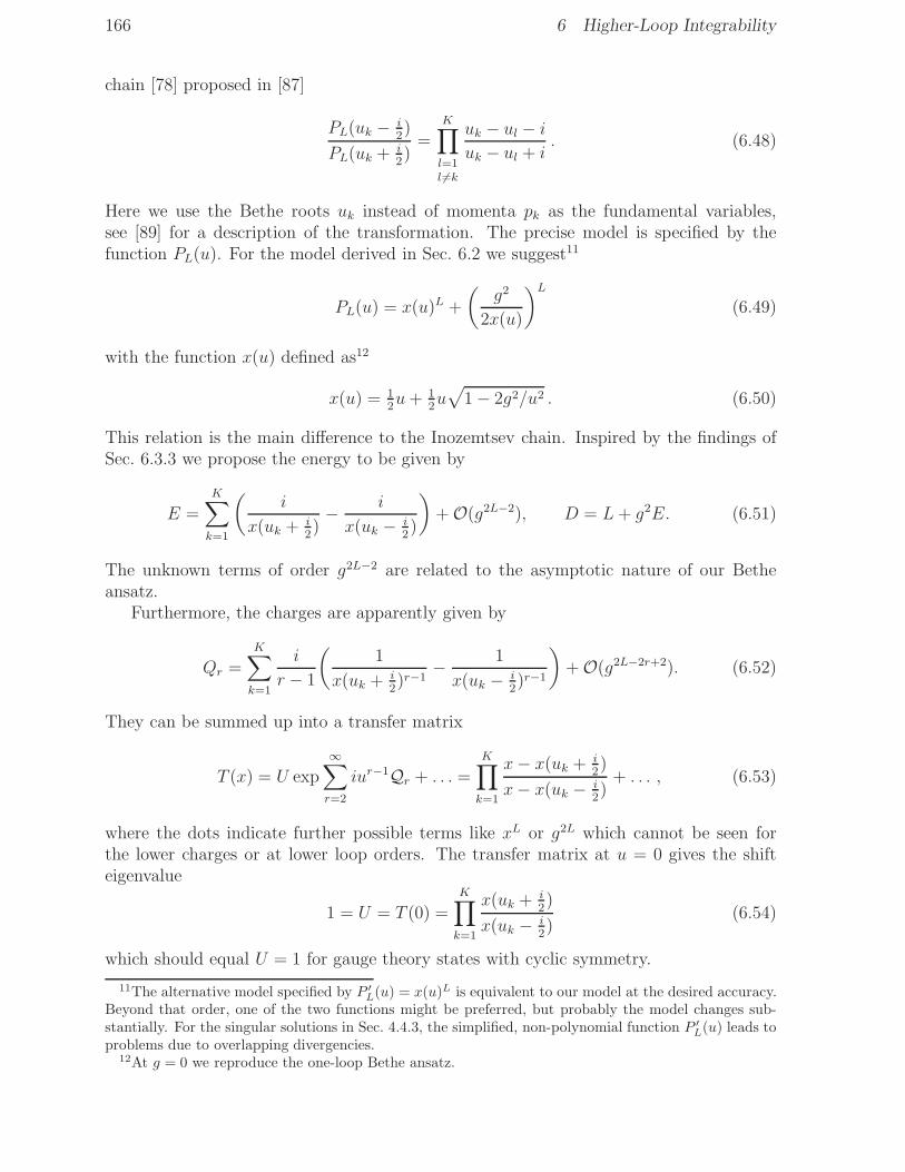
166 6 Higher-Loop Integrability
chain [78] proposed in [87]
PL(uk − i2)
PL(uk + i2)
=
K∏
l=1l 6=k
uk − ul − iuk − ul + i
. (6.48)
Here we use the Bethe roots uk instead of momenta pk as the fundamental variables,see [89] for a description of the transformation. The precise model is specified by thefunction PL(u). For the model derived in Sec. 6.2 we suggest11
PL(u) = x(u)L +
(g2
2x(u)
)L(6.49)
with the function x(u) defined as12
x(u) = 12u+ 1
2u√
1− 2g2/u2 . (6.50)
This relation is the main difference to the Inozemtsev chain. Inspired by the findings ofSec. 6.3.3 we propose the energy to be given by
E =
K∑
k=1
(i
x(uk + i2)− i
x(uk − i2)
)+O(g2L−2), D = L+ g2E. (6.51)
The unknown terms of order g2L−2 are related to the asymptotic nature of our Betheansatz.
Furthermore, the charges are apparently given by
Qr =K∑
k=1
i
r − 1
(1
x(uk + i2)r−1− 1
x(uk − i2)r−1
)+O(g2L−2r+2). (6.52)
They can be summed up into a transfer matrix
T (x) = U exp
∞∑
r=2
iur−1Qr + . . . =
K∏
k=1
x− x(uk + i2)
x− x(uk − i2)
+ . . . , (6.53)
where the dots indicate further possible terms like xL or g2L which cannot be seen forthe lower charges or at lower loop orders. The transfer matrix at u = 0 gives the shifteigenvalue
1 = U = T (0) =
K∏
k=1
x(uk + i2)
x(uk − i2)
(6.54)
which should equal U = 1 for gauge theory states with cyclic symmetry.
11The alternative model specified by P ′L(u) = x(u)L is equivalent to our model at the desired accuracy.
Beyond that order, one of the two functions might be preferred, but probably the model changes sub-stantially. For the singular solutions in Sec. 4.4.3, the simplified, non-polynomial function P ′
L(u) leads toproblems due to overlapping divergencies.
12At g = 0 we reproduce the one-loop Bethe ansatz.

6.4 Long-Range Bethe Ansatz 167
The function PL(u) is indeed a polynomial of degree L in u, which can be derived fromthe inverse of (6.50)
u(x) = x+g2
2x. (6.55)
Therefore, the equation (6.48) is the Bethe equation of an inhomogeneous spin chain, seeSec. 4.1.2 and [59]. The polynomial can be factorised and we obtain for the inhomo-geneities vp
PL(u) =L∏
p=1
(u− vp) with vp =√
2 g cosπ(2p− 1)
2L. (6.56)
Now it can be noticed that the physical transfer matrix T (x) is not the natural transfermatrix T ′(u) associated to the inhomogeneous spin chain
T ′(u) =K∏
k=1
u− uk − i2
u− uk + i2
+PL(u)
PL(u+ i)
K∏
k=1
u− uk + 3i2
u− uk + i2
. (6.57)
The Bethe equations follow from this transfer matrix by cancellation of poles at uk − i2.
The charges Q′r derived from T ′(u) are given as in (4.54). In perturbation theory we can
relate these charges to the physical charges Qr by
Qr = Q′r + 1
2(r + 1)g2Q′
r+2 + 18(r + 2)(r + 3)g4Q′
r+4 + . . . . (6.58)
Let us first of all comment on the inhomogeneity. Our spin chain is homogeneous,how can the Bethe ansatz of an inhomogeneous spin chain describe our model? Firstof all, the equation (6.58) is merely an eigenvalue equation, it does not directly relatethe homogeneous and inhomogeneous charges, Qr and Q′
s; it merely tells us that thereis a similarity transformation between the two. Similar maps are encountered within theinhomogeneous spin chain itself: On the one hand, the order of the inhomogeneities vpdoes not matter for the Bethe ansatz and thus for the eigenvalues Q′
r of the charges. Onthe other hand, it should certainly influence the charge operators Q′
r. Consequently, theeigenstates should be related by a similarity transformation.13 To understand our modelbetter, it would be essential to investigate this point further and find the map betweenour homogeneous spin chain model and the common inhomogeneous spin chain.
In our equations, the map between x and u (6.50,6.55) plays a major role. It is adouble covering map, for every value of u there are two corresponding values of x, namely
u←→{x,g2
2x
}. (6.59)
For small values of g, where the asymptotic Bethe ansatz describes the long-range spinchain, we will always assume that x ≈ u. When g is taken to be large (if this makessense at all is a different question), however, special care would be needed in selecting theappropriate branch. The double covering map for x and u has an analog for the transfermatrices T (x) and T ′(u). We find the relation
T (x)T (g2/2x)
T (0, g)≈ T ′(u). (6.60)
13The inhomogeneities vp and vp+1 can be interchanged by conjugation with Rp,p+1(vp − vp+1).

168 6 Higher-Loop Integrability
which holds if the second term in (6.57) is dropped. It can be proved by using the doublecovering relation
(x− x′)(
1− g2
2xx′
)=
(x+
g2
2x
)−(x′ +
g2
2x′
)= u− u′. (6.61)
We believe it is important to further study the implications of the double covering maps.This might lead to insight into the definition of our model, possibly even beyond wrappingorder.
Now we have totally self-consistent Bethe equations with associated transfer matrixelements T ′(u). Unfortunately, T ′(u) does not directly describe physical quantities, suchas the energy E. These are encoded in the physical transfer matrix elements T (x) whichinvolve the function x(u) and are ambiguous due to the two branches of the square root.This is not a problem in perturbation theory, however, even there inconsistencies areobserved at higher order in g [89]. Remarkably, these appear precisely at the orderwhere wrapping interactions start to contribute and our asymptotic Bethe ansatz is fullyconsistent to the desired accuracy. Conversely, there are signs of the missing of wrappingterms. We hope that finding a cure for the problems beyond wrapping order mighthelp to find a generalization of the Bethe equations which include wrapping interactions.Presumably these equations will have a substantially different form, see Sec. 6.4.4.
6.4.2 Results
Here we summarise the results of a comparison of the above Bethe ansatz with thespectrum of the spin chain model. For the details of the comparison we refer the readerto the article [89].
• The energy of states with two excitations agrees with the formula given in Tab. 6.10.In fact, the five-loop result was obtained using the Bethe ansatz, where this is astraightforward task. It was shown to agree with the model in a number of cases.Furthermore, it is possible to derive all-loop results in the near BMN limit. Theenergy as an analytic function in λ′ is indeed given by the conjectured formula (6.42).
• The general BMN energy formula (3.99,3.98) is easily confirmed.
• The unpaired three-excitation states are singular. We can treat these solutions bydemanding cancellation of singularities in the transfer matrix T ′(u). Remarkably, theresults agree with their respective mirror solutions, see Sec. 4.3.1. These have L − 2excitations instead of 3 and are regular. Up to L = 10 their energies do agree with(6.44).
• All states with L ≤ 8 and all unpaired ones with L ≤ 10 have been computed in theBethe ansatz. Their energies agree with Tab. 6.8.
• We have also compared some higher charges of the Bethe ansatz with the correspondingexplicit computations. They agree.
In conclusion, we can say that for all considered examples, the Bethe ansatz yieldsprecisely the same spectrum as the integrable spin chain model constructed in Sec. 6.2.It shows that an integrable spin chain with a well-defined thermodynamic limit (see

6.4 Long-Range Bethe Ansatz 169
Sec. 6.1.5) is very likely to exist in contrast to the doubts raised in [87]. In terms ofthe long-range Bethe ansatz there may seem to be many such models. These wouldbe obtained by replacing the phase relation (6.49) and energy formula (6.51) by someother function that is well-behaved in the limit. If we however demand that the modelis related to an inhomogeneous spin chain, we find a unique model with thermodynamicscaling behaviour, see [89] for details.
The upshot for the integrable spin chain model is similar: In its construction we haveassumed a very specific form of interactions and the obtained Hamiltonian has turnedout to be unique (at five loops). In other words, the very relations (6.49,6.51) are specialand correspond to the assumed form of interactions (iii).14 At any rate, the relations(6.49,6.51) are very suggestive in view of a correspondence to string theory on plane waves,see Sec. 3.6. It is therefore not inconceivable, that the Bethe ansatz indeed describes planarN = 4 gauge theory in the su(2) subsector at higher-loops.
6.4.3 The Thermodynamic Limit
Here we shall only present the thermodynamic limit of the equations in (6.4.1). Theoverall structure is the same as described in Sec. 4.5 only that we now introduce depen-dence on the effective coupling constant
g = g/L. (6.62)
An application and sample calculation is found in [89].As before, we shall assume that the roots uk = uk/L condense on a disconnected
contour C in the complex plane with density function ρ(u). The density is again normalisedby the total filling fraction K = K/L
∫
Cdu ρ(u) = K. (6.63)
We find for the energy and the momentum constraint
E =
∫
C
du ρ(u)
u√
1− 2g2/u2
1
x(u), 2πn =
∫
C
du ρ(u)
u√
1− 2g2/u2, (6.64)
with the map between x and u is given by15
x(u) = 12u+ 1
2u√
1− 2g2/u2 , u(x) = x+g2
2x, (6.65)
whereas the higher-loop generalisation of the Bethe equation reads
2πnu −1
u√
1− 2g2/u2= 2 −
∫
C
dv ρ(v)
v − u . (6.66)
In the thermodynamic limit, the physical charges and resolvent are given by
Qr =
∫
C
du ρ(u)
u√
1− 2g2/u2
1
x(u)r−1, G(x) =
∫
C
du ρ(u)
u√
1− 2g2/u2
x(u)
x(u)− x . (6.67)
14This picture is rather similar to the Inozemtsev spin chain where the requirement of pairwise inter-actions of spins at a distance was shown to lead to the phase relation of the Inozemtsev-Bethe ansatz.
15Note the useful identity x− g2/2x = u√
1− 2g2/u2 .

170 6 Higher-Loop Integrability
As in the one-loop case, the Bethe equation (6.66) can alternatively be written as aconsistency condition on the singular transfer matrix T ′(u) ∼ 2 cosG′
sing(u) with
G′sing(u) = G′(u) +
1
2u√
1− 2g2/u2and G′(u) =
∫
C
dv ρ(v)
v − u . (6.68)
The function 2 cosG′sing(u) is single-valued if it obeys (4.113)
G′sing(u+ iǫ) +G′
sing(u− iǫ) = 2πnu (6.69)
across a cut of G′ at u. At this point, it is however not clear how the physical transfermatrix T (x) is related to the physical resolvent G(x) and if there is also a consistencyrequirement which leads to the Bethe equations. This is largely related to mirror cuts inT (g2/2x) which are due to the double covering map (6.61).
6.4.4 Bethe Ansatze for Bigger Subsectors
The Bethe ansatz has proved to be a very powerful tool in obtaining the spectrum athigh loop orders. It would therefore be extremely interesting and important to generaliseit to bigger subsectors than the su(2) subsector, preferably to the complete psu(2, 2|4)spin chain. Despite some attempts we have not succeeded in finding suitable equationsbeyond the su(2) sector.16 We would thus like to present a number of considerations forthe construction of a complete all-loop Bethe ansatz.
• The most important issue seems to be multiplet shortening, see also Sec. 1.8,4.3.5.The spectrum contains a number of multiplets which are short in the free theory. Ashort multiplet cannot acquire an anomalous dimension (energy) unless it combineswith other short multiplets to form a long one (in analogy to the Higgs mechanism).
The one-loop Bethe ansatz was not constructed to respect multiplet joining, never-theless it does display this feature. For all short, non-protected multiplets compatibleshort multiplets can be found. All of these have not only equal anomalous dimensionbut also equal higher charges so that they can join in the interacting theory. Theone-loop Bethe ansatz has a solution for all highest-weight states of the multiplets. Inparticular, there are multiple solutions for splitting multiplets. At higher-loops thesemultiplets join, consequently the complete Bethe ansatz should only find the highestweight of the long multiplet. The highest weights of the submultiplets should notgeneralise or display some other kind of inconsistency beyond one-loop.
• There is another issue related to multiplet shortening. The Bethe ansatz not onlyyields solutions corresponding to gauge theory states, but also solutions with non-zeromomentum, U 6= 1. A naive generalisation to higher-loops would also produce thesestates. This, however, would be inconsistent for a simple reason: Short multiplets inthe non-zero momentum sector generically do not have suitable partners to join up.Let us consider the state
|X〉 = |Zφ〉 − |φZ〉. (6.70)
This state does not obey the momentum constraint, i.e. Tr |X〉 = 0 or U|X〉 = −|X〉.It is not physical, but nevertheless reproduced by the Bethe ansatz. Its Dynkin labels
16In the thermodynamic limit there are simplifications which allow to guess the Bethe equations [132].

6.5 Stringing Spins at Higher Loops 171
are [0; 0; 1, 0, 1; 0; 0], it is the primary of a BPS multiplet. In principle this multipletcould join with another short multiplet of lower dimension to form a long one. Herethis is not possible, there are no potential partners. Consequently, this multipletwould have to be protected, but a direct computation using the one-loop Hamiltonianor Bethe ansatz yields E = 4 which is inconsistent. A prospective Bethe ansatz shouldtake this into account and exclusively yield solutions with zero momentum.
• There is a complication which applies to non-compact and supersymmetric represen-tations: The Dynkin labels r, r1, r2 contain the anomalous dimension δD and thuschange with g. For the Bethe ansatz, the labels also specify the number of excitationsfor any given state (c.f. Sec. 4.3.4) which certainly must be positive integers. It isnot clear if and how these two points can be combined. If possible, it is reasonableto believe that the Bethe equations will be a self-consistency equation on the energy(this is somewhat similar to the integral equations which appear in string theory [75]).In perturbation theory at each order, the corrected energy would have to be used asinput for the next order.
• The length L and hypercharge B are not good quantum numbers in dynamic spinchains. However, they are also used as input for the Bethe equations, see Sec. 4.3.4.It is not clear how to identify states when L and B cannot be fixed; ideally the Betheansatz for a dynamic spin chain should not distinguish between states with differentL,B.
All in all this suggests that the prospective all-loop psu(2, 2|4) Bethe ansatz, if it exists,17
has a rather different structure than the one-loop approximation. Even more, the one-loop ansatz might turn out not to be a smooth limit of it. This could indeed be a blessingin disguise because a substantially different Bethe ansatz might allow for the inclusion ofwrapping interactions, see Sec. 6.5.4 or even incorporate them naturally.
The arguments presented above do not apply to the su(2) subsector because there isno multiplet shortening and the su(2) labels are not affected by the anomalous dimension.This explains why it was relatively easy to find our all-loop generalisation.
For a generalisation one might take a more pragmatic point of view and merely considerthe classical algebra as the symmetry algebra. All classical representation labels wouldbe perfectly well-defined and integer. The Bethe ansatz should yield some energies whichwe interpret as the corrections to the scaling dimensions. It would then be essential thatall submultiplets have precisely the same energy and charges. Solutions with non-zeromomentum would have to be ignored. The only shortcoming of such an ansatz would bethat it does not explain the truly interacting structure of the algebra.
6.5 Stringing Spins at Higher Loops
Now that we have a Bethe ansatz for higher-loop scaling dimensions we may continuethe comparison of spinning strings and gauge theory started in Sec. 4.6.
17Given that N = 4 SYM is likely to be an integrable model, even beyond one-loop, we can hope forsome associated Bethe ansatz.
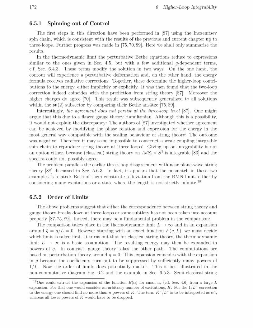
172 6 Higher-Loop Integrability
6.5.1 Spinning out of Control
The first steps in this direction have been performed in [87] using the Inozemtsevspin chain, which is consistent with the results of the previous and current chapter up tothree-loops. Further progress was made in [75, 70, 89]. Here we shall only summarise theresults.
In the thermodynamic limit the perturbative Bethe equations reduce to expressionssimilar to the ones given in Sec. 4.5, but with a few additional g-dependent terms,c.f. Sec. 6.4.3. These terms modify the solution in two ways. On the one hand, thecontour will experience a perturbative deformation and, on the other hand, the energyformula receives radiative corrections. Together, these determine the higher-loop contri-butions to the energy, either implicitly or explicitly. It was then found that the two-loopcorrection indeed coincides with the prediction from string theory [87]. Moreover thehigher charges do agree [70]. This result was subsequently generalized to all solutionswithin the su(2) subsector by comparing their Bethe ansatze [75, 89].
Interestingly, the agreement does not persist at the three-loop level [87]. One mightargue that this due to a flawed gauge theory Hamiltonian. Although this is a possibility,it would not explain the discrepancy: The authors of [87] investigated whether agreementcan be achieved by modifying the phase relation and expression for the energy in themost general way compatible with the scaling behaviour of string theory: The outcomewas negative. Therefore it may seem impossible to construct a weak coupling integrablespin chain to reproduce string theory at ‘three-loops’. Giving up on integrability is notan option either, because (classical) string theory on AdS5×S5 is integrable [83] and thespectra could not possibly agree.
The problem parallels the earlier three-loop disagreement with near plane-wave stringtheory [88] discussed in Sec. 5.6.3. In fact, it appears that the mismatch in these twoexamples is related: Both of them constitute a deviation from the BMN limit, either byconsidering many excitations or a state where the length is not strictly infinite.18
6.5.2 Order of Limits
The above problems suggest that either the correspondence between string theory andgauge theory breaks down at three-loops or some subtlety has not been taken into accountproperly [87, 75, 89]. Indeed, there may be a fundamental problem in the comparison:
The comparison takes place in the thermodynamic limit L→∞ and in an expansionaround g = g/L = 0. However starting with an exact function F (g, L), we must decidewhich limit is taken first. It turns out that for classical string theory, the thermodynamiclimit L → ∞ is a basic assumption. The resulting energy may then be expanded inpowers of g. In contrast, gauge theory takes the other path. The computations arebased on perturbation theory around g = 0. This expansion coincides with the expansionin g because the coefficients turn out to be suppressed by sufficiently many powers of1/L. Now the order of limits does potentially matter. This is best illustrated in thenon-commutative diagram Fig. 6.2 and the example in Sec. 6.5.3. Semi-classical string
18One could extract the expansion of the function E(α) for small α, (c.f. Sec. 4.6) from a large Lexpansion. For that one would consider an arbitrary number of excitations, K. For the 1/Ln correctionto the energy one should find no more than n powers of K. The term Kn/Ln is to be interpreted as αn,whereas all lower powers of K would have to be dropped.
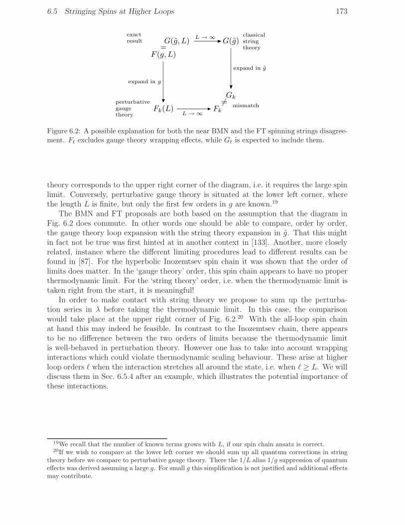
6.5 Stringing Spins at Higher Loops 173
F (g, L)=G(g, L)
Fk(L)
G(g)
Fk
6=Gk
classicalstringtheory
mismatchperturbativegaugetheory
exactresult
expand in g
expand in g
L → ∞
L → ∞
Figure 6.2: A possible explanation for both the near BMN and the FT spinning strings disagree-ment. Fℓ excludes gauge theory wrapping effects, while Gℓ is expected to include them.
theory corresponds to the upper right corner of the diagram, i.e. it requires the large spinlimit. Conversely, perturbative gauge theory is situated at the lower left corner, wherethe length L is finite, but only the first few orders in g are known.19
The BMN and FT proposals are both based on the assumption that the diagram inFig. 6.2 does commute. In other words one should be able to compare, order by order,the gauge theory loop expansion with the string theory expansion in g. That this mightin fact not be true was first hinted at in another context in [133]. Another, more closelyrelated, instance where the different limiting procedures lead to different results can befound in [87]. For the hyperbolic Inozemtsev spin chain it was shown that the order oflimits does matter. In the ‘gauge theory’ order, this spin chain appears to have no properthermodynamic limit. For the ‘string theory’ order, i.e. when the thermodynamic limit istaken right from the start, it is meaningful!
In order to make contact with string theory we propose to sum up the perturba-tion series in λ before taking the thermodynamic limit. In this case, the comparisonwould take place at the upper right corner of Fig. 6.2.20 With the all-loop spin chainat hand this may indeed be feasible. In contrast to the Inozemtsev chain, there appearsto be no difference between the two orders of limits because the thermodynamic limitis well-behaved in perturbation theory. However one has to take into account wrappinginteractions which could violate thermodynamic scaling behaviour. These arise at higherloop orders ℓ when the interaction stretches all around the state, i.e. when ℓ ≥ L. We willdiscuss them in Sec. 6.5.4 after an example, which illustrates the potential importance ofthese interactions.
19We recall that the number of known terms grows with L, if our spin chain ansatz is correct.20If we wish to compare at the lower left corner we should sum up all quantum corrections in string
theory before we compare to perturbative gauge theory. There the 1/L alias 1/g suppression of quantumeffects was derived assuming a large g. For small g this simplification is not justified and additional effectsmay contribute.
174 6 Higher-Loop Integrability
6.5.3 Example
Here we present an example where one can see the importance of the order of limits.We choose a function
F (g, L) =g2L
(c+ g2)L=
(1 +
c
g2L2
)−L= G(g, L). (6.71)
In perturbation theory around g = 0 we find that the function vanishes at L leading looporders
F (g, L) =∞∑
k=0
Fk gk =
g2L
cL− g2L+2
cL+1+g2L+4
cL+2+ . . . , i.e. Fk(L) = 0 for k < 2L.
(6.72)The leading factor g2L mimics the effect of wrapping interactions in gauge theory asexplained below. When we now go to the thermodynamic limit, L→ ∞, we see that allcoefficients Fk are zero.
Now let us take the thermodynamic limit first. The large L limit ofG(g, L) =∑
kGk gk
yields G(g) = 1 in a straightforward fashion. This result depends crucially on the functionF (g, L). Currently, we do not know how to incorporate wrapping interactions, but g2L
alone would not have a sensible thermodynamic limit. To compensate this, we haveintroduced some function 1/(c+ g2)L. Clearly we cannot currently prove that gaugetheory produces a function like this, but it appears to be a definite possibility. In our toyexample, the expansion in g gives G0 = 1 and Gk = 0 otherwise.
In conclusion we find G0 = 1 while F0 = 0 which demonstrates the non-commutativityof the diagram in Fig. 6.2 in an example potentially relevant to our context. It is not hardto construct a function F (g, L) which yields arbitrary coefficients Gk while all Fk remainzero.
Note however that there is a sign of the non-commutativity in (6.72): A correct scalingbehaviour would require the coefficient Fk to scale as L−k. In particular for k = 2L, thecoefficient should scale as L−2L instead of c−L. Therefore one can say that the function Fviolates the scaling law even at weak coupling, but in a mild way that is easily overlooked.This parallels the above observations for the Inozemtsev spin chain that a proper scalingbehaviour might be obscured in perturbation theory.
6.5.4 Wrapping Interactions
One very important aspect of the spin chain are wrapping interactions (c.f. Sec. 2.6.3).These interactions appear when the expected length of the interactions, ℓ+1, exceeds thelength of the state L. Let us note that the asymptotic Bethe ansatz for the Inozemtsevspin chain apparently does not incorporate wrapping interactions correctly. As our ansatzis very similar, we expect the same to apply here.
For a fixed length L, the wrapping interactions are irrelevant at lower loop orders, butat higher-loops they are the only contribution. Therefore, at finite values of the couplingconstant, wrapping interactions dominate and the dependence on the coupling constantmay change completely. This is very appealing from the point of view of the AdS/CFTcorrespondence, which predicts the scaling dimension of a generic, unprotected state togrow like
√g ∼ λ1/4 for large g [5].Instead, the energy formula (6.51) seems to suggest
6.5 Stringing Spins at Higher Loops 175
a linear growth in g, but it is valid only for sufficiently low loop orders. Therefore wesuspect that wrapping interactions may be responsible for the conjectured
√g behaviour
at large g. Note that a generalisation of the Bethe equations for classical string theory [75]to towards the quantum regime has been conjectured in [130]. These equations reproducethe λ1/4 behaviour as well as the near plane wave results of [88, 129, 102,131].
In the same spirit, wrappings may be important for the comparison between gaugetheory and string theory in the case of spinning strings and the near BMN limit [89]where they become an order-of-limits issue: When we assume the length of the state tobe sufficiently large, wrapping interactions are suppressed. Then we find that g and 1/Lcombine and the energy is a function of g. However, for a comparison to string theory,we might wish to take g finite for a fixed length. Again we should find that g and 1/Lcombine (possibly for a completely different reason) and obtain a function of g. Herewe may expect a qualitative difference because wrappings dominate the complete tail ofthe perturbative expansion for any fixed length. Summing up the perturbative series wemight get a totally different function, as demonstrated by the example in Sec. 6.5.3.
Unfortunately, we currently have no handle on wrapping interactions. In the alge-braic analysis of Ch. 5, there seem to be few constraints on their form. In fact, virtuallyany higher-loop anomalous dimensions can be assigned to multiplets with a small lengthby means of wrapping interactions. For the Bethe ansatz the inclusion of wrapping in-teractions will probably require a substantially different form. For instance, an exact,non-asymptotic Bethe ansatz for the Inozemtsev chain is not known [78].
All in all, a better understanding of wrapping interactions might be of great importanceto the AdS/CFT correspondence and our understanding of higher-loop conformal gaugetheory.

176

177
Conclusions
In this dissertation we have developed means to efficiently compute and investigatescaling dimensions of local operators in a perturbative four-dimensional conformal fieldtheory. The central object is the dilatation operator ; it is one of the generators of the(super)conformal algebra and it measures scaling dimensions. In the example of N = 4supersymmetric gauge theory, we have made use of the symmetry algebra and structuralproperties of Feynman graphs to derive this generator up to a few quantum loops; theanalysis is purely algebraic, no actual (higher-loop) computations were required. Theobtained results have allowed us to prove that the planar dilatation operator is completelyintegrable, not only at one-loop, but possibly even at higher-loops and for finite values ofthe coupling constant.
Apart from generic interest in the structure of field theories at higher-loops, our investi-gations are motivated by the AdS/CFT correspondence. One prediction of this conjectureis the agreement of the spectrum of scaling dimensions of local operators in N = 4 SYMwith the spectrum of energies of IIB string theory on AdS5 × S5. The dilatation op-erator has become a versatile tool for testing and even proving parts of the AdS/CFTcorrespondence.
There are various ways to deduce scaling dimensions of local operators and theirquantum corrections (i.e. the anomalous dimensions) from field theory correlators. Theyare convenient when interested in particular and rather simple local operators at low looporders. Unfortunately, the AdS/CFT correspondence relates this regime of operatorsto an essentially inaccessible strong-coupling regime in string theory. Conversely, theperturbative regime of string theory is usually mapped to an inaccessible regime in gaugetheory. In recent years, it has emerged that this incompatibility can be overcome whenfocusing on states with a large spin quantum number on S5, or equivalently of so(6). Ingauge theory this requires operators with a large number of constituents in which case thedirect approach requires too much work. It is therefore desirable to have some technologyto deal with such states in an efficient way.
The dilatation generator is perfectly suited to investigate scaling dimensions. As com-pared to conventional methods, it offers several advantages: Once it is obtained from fieldtheory, the computation of scaling dimensions is turned into a combinatorial exercise.Furthermore, the dilatation operator is an algebraic object and one can save a significantamount of work by simplifying it, before it is applied to specific states. Moreover, one cantry to obtain the dilatation operator without performing labourious field theory computa-tions; this constitutes one of the key results of the current work. Finally, whereas scalingdimensions are just a set of data, the dilatation generator comprises the whole spectrum;it allows to compare on an abstract level and thus prove the equivalence of certain spec-tra instead of performing tests for an (inevitably small) set of states. For instance, when

178 Conclusions
non-planar corrections are taken into account, the dilatation generator can split and jointraces (alias strings) making it very reminiscent of a stringy Hamiltonian. What is more,in N = 4 SYM in the BMN limit, it was shown to coincide also quantitatively with theplane-wave string field theory Hamiltonian. This proves the agreement of arbitrary-genuscontributions to scaling dimensions/energy and constitutes a strong test of the AdS/CFTor plane-wave/BMN correspondence.
Here, we have chosen N = 4 supersymmetric gauge theory as a model quantum con-formal field theory in four spacetime dimensions. For this model we have first investigatedthe dilatation operator in the one-loop approximation. We have started by making themost general ansatz compatible with field theory, which involves infinitely many unde-termined coefficients. Subsequently, we have used conformal invariance to reduce theindependent coefficients, first to one infinite sequence, then to just a single one. Beingrelated to a rescaling of the coupling constant, it is not possible to assign a value to theleftover coefficient except by actually computing it in field theory. Therefore, the com-plete one-loop dilatation operator of N = 4 SYM is entirely fixed by symmetry (up toobvious transformations).
Similar conclusions hold also at higher-loops: A general treatment would have requiredvery much work, therefore we have first investigated subsectors on which the dilatationoperator closes. In an interesting one, the su(2|3) subsector, we were able to obtain planarthree-loop corrections by algebraic means. Again, the result has turned out to be uniqueup to symmetries of the defining relations. This enables us to perform a very exact test ofAdS/CFT correspondence and the near plane-wave/BMN limit thereof. Remarkably, thistest has revealed a discrepancy starting only at three-loops. We have presented a possibleexplanation in terms of an order of limits problem, but more importantly, it demonstratesthat we can find relevant and unexpected physics even in a higher-loop computation!
The dilatation operator is not only useful to obtain scaling dimensions, but it is inter-esting in itself. One exciting feature of the planar dilatation operator, with very importantconsequences, is its apparent integrability. As far as the spectrum is concerned, integrabil-ity merely leads to a curiosity: For generic multiplets of local operators there is a partnerwith exactly degenerate anomalous dimension. Below the surface, however, the existenceof arbitrarily many conserved commuting charges strongly constrains the dilatation op-erator. This leads to a major simplification in computing scaling dimensions due to thealgebraic Bethe ansatz.
The Bethe ansatz is especially powerful in the thermodynamic limit, i.e. for local op-erators with a large number of constituent fields. This limit is practically inaccessibleby conventional methods, however, here the Bethe equations turn into integral equationswhich can still be solved in practice. The AdS/CFT correspondence relates the thermo-dynamic limit of N = 4 SYM to classical spinning string configurations on AdS5 × S5.The energy is usually given by intricate algebraic, elliptic or hyperelliptic functions ofthe ratios of the involved spins. In a number of cases, agreement between gauge theoryand string theory could be shown, which confirms the correspondence with unprecedentedaccuracy. Even more, the Bethe equations in the thermodynamic limit could be shownto coincide with integral equations derived from string theory!
Integrability of the planar dilatation operator was first found at one-loop and forcertain subsectors of states. More accurately, it was shown that the dilatation operatoris isomorphic to the Hamiltonian of an integrable quantum spin chain with so(6) or
Conclusions 179
sl(2) symmetry. In this work we have extended these one-loop results to the completespectrum of states and full psu(2, 2|4) superconformal symmetry. Even more exciting isa generalisation of integrability to higher-loops, an entirely new topic. We have foundseveral indications for integrability beyond one-loop although a framework to investigate,prove and exploit it, is yet to be established. Most importantly, the three-loop correctionsto the dilatation operator within the su(2|3) subsector preserve the above-mentioneddegeneracy of pairs. Furthermore, the integrable spin chain due to Inozemtsev reproducesthree-loop planar scaling dimensions correctly. Finally, the sigma model of string theoryon AdS5 × S5 is integrable and, via the AdS/CFT correspondence, one expects the samefeature for the corresponding gauge theory.
In order to investigate higher-loop integrability, we have constructed a deformation ofthe Heisenberg integrable spin chain model. The assumed form of interactions is inspiredby field theory and conjectures about N = 4 SYM. If all our conjectures are justified,the model will describe planar anomalous dimensions. Independently of that question,the model displays some remarkable features: Our assumptions have turned out to besufficiently constraining such that we obtain a unique result up to at least five-loops.Intriguingly, it reproduces the BMN energy formula correctly. Moreover, we have founda long-range Bethe ansatz, very similar to the one describing the Inozemtsev spin chain,which reproduces the spectrum of the spin chain exactly. But this is not all: It is validfor all loop orders, at least if the spin chain is sufficiently long! Have we hereby openedup a window for finite coupling constant?
In conclusion, we have presented a versatile technology to investigate scaling dimen-sions in a conformal field theory. We have completed the one-loop calculation and evenhad a glimpse of higher-loop physics. Hopefully, making full use of integrability will finallyallow us to leave the weak coupling regime.

180

181
Outlook
There is a wide range of open questions and problems which can be addressed withthe ideas and methods presented in this work; we will group them according to the topicspresented in the individual chapters. Let us start with the dilatation operator in generalwhich has been considered in Ch. 2:
• It would be very helpful to develop techniques, similar to the ones presented here,for the efficient evaluation of structure constants of the operator product expansion,see Sec. 1.10. Apart from the scaling dimensions, they are the other central quan-tity in a conformal field theory of local operators. The structure constants may beobtained from three-point functions, but a direct computation is ‘contaminated’ byuseless finite and divergent contributions from the perturbative expansion of the scal-ing dimensions. One therefore wonders whether one may generalise our methodologyand develop purely algebraic techniques for directly finding the structure constants.See e.g. [134] for some work in that direction. Especially within the BMN three-pointfunctions are important for the comparison to the plane-wave string theory [135],c.f. [108, 21, 22, 136, 49] for some results.
• It might be interesting to extend the current analysis to non-perturbative effects likeinstantons. Possibly the symmetry algebra also puts constraints on these and a directcomputation as in [137] might be simplified or even bypassed.
In Ch. 3 we have investigated the dilatation operator at one-loop:
• We have focussed on N = 4 SYM in this work, but there are a few further four-dimensional conformal quantum field theories with N = 2 supersymmetry. For these,the determination of the dilatation generator might shed some light on holographicdualities away from the well-studied case of AdS5 × S5. Even if the superconformalalgebra is smaller, we expect that it is similarly constraining and our results shouldgeneralise in a rather straightforward fashion. Some advances in this direction havebeen made in e.g. [138, 139].
• Even in a QFT with broken conformal invariance [56], the techniques developed inthis work can be used to investigate logarithmic corrections to two-point functionsand scattering amplitudes in a systematic way. In particular in QCD at large Nc anddeep inelastic scattering, similar techniques are at use (see e.g. [52–55]).
Questions related to the dilatation operator at higher-loops in Ch. 5:
• The complete one-loop contribution to the dilatation operator has turned out to betotally fixed by superconformal symmetry; the same might apply at two or even higher-
182 Outlook
loops. This conjecture is not unreasonable, as the action is unique and entirely de-termined by psu(2, 2|4). Whether or not the conjecture is true, it would be great toderive the complete two-loop deformation.
• In Ch. 3,5 we have considered the algebras psu(2, 2|4) and su(2|3) with the fundamentalfields transforming in certain representations. An interesting mathematical questionis, which algebras and representations are suited for consistent deformations of thealgebra generators? Are they all related to (conformal) field theories?
• A very important issue is the form of wrapping interactions. For those, our methodsappear to be not very constraining at higher loop orders. A non-planar treatmentmight solve the problem, but the complexity will increase drastically due to the largeamount of such digrams. For operators of a finite length, wrappings dominate the tailof the perturbation series. They are therefore of tremendous importance for the finitecoupling regime.
• It would be nice to confirm some of the higher-loop results of this work explicitly infield theory. Although we believe our computations are rigorous, we had to rely onsome basic assumptions (e.g. the BMN-limit) which are not firm facts of gauge theoryyet.
• A curious observation is that all the anomalous dimensions we have found are solutionsto algebraic equations. In contrast, higher-loop amplitudes usually involve transcen-dental numbers such as ζ(3), ζ(5), . . . . Are these merely a renormalisation artefact ordo they appear at some higher loop order?
A related question is whether the coupling constant is renormalised by a finite amount.For instance, this happens in the BMN matrix model (c.f. Sec. 2.1.6), where a redef-inition of the coupling constant is required to achieve a proper scaling in the BMNlimit [79] (it is a non-trivial result that this is possible at all).
One-loop integrability was the subject of Ch. 4:
• Clearly, the deep question is, why does integrability emerge from the planar N = 4gauge theory? Of course, via the the AdS/CFT correspondence, one could take inte-grability of the classical string sigma model [82–84] as compelling evidence, neverthe-less we believe there should also be an intrinsically field theoretical reason.
• We know that the spectrum of Q2 is related to the spectrum of anomalous dimensions.A natural question to ask is whether the spectra of the higher charges Qr have aphysical meaning in the gauge theory.
• Integrability implies the appearance of degenerate pairs in the planar spectrum due toan interplay of two charges and parity. However, there appears to be no deeper reasonfor the pairs in terms of representation theory. It would be very desirable to understandthe degeneracy of pairs better, in terms of N = 4 SYM as well as in terms of theAdS/CFT correspondence. A possible explanation would be that symmetry extendsby some compact SO(2) group whose representations are either uncharged singletsor charged doublets. The integrable charges Qr are not suitable SO(2) generatorsbecause their spectrum is non-integer. The SO(2) symmetry naturally combines withthe parity Z2 to O(2) and 1/N corrections break it to Z2.

Outlook 183
Could the conjectured SO(2) symmetry be related to the conjectured modular invari-ance of N = 4 SYM? In the unbroken form, SL(2,R), the SO(2) subgroup of modularinvariance would pair up states. When broken to SL(2,Z) by higher-genus corrections,there is no SO(2) group to protect the pairing and the degeneracy is lifted.
• Integrability seems to apply to a wider range of field theories. The obvious candidatesare conformal field theories, see e.g. [140]. However, in theories where conformal invari-ance is broken by quantum effects, such as massless QCD, one may still investigate theone-loop dilatation operator, for which conformal symmetry applies, see e.g. [139,141].In QCD, following pioneering work of Lipatov [52], methods of integrability have alsohad much impact, see e.g. [53–55].
• On the one hand, we have demonstrated in Sec. 3.3 that the superconformal algebraleads to a unique one-loop anomalous dilatation operator. On the other hand, thereis a unique standard spin chain Hamiltonian with psu(2, 2|4) symmetry. In fact, bothoperators turn out to be the same, which shows that conformal symmetry and inte-grability go hand in hand. This is remarkable because we consider a four-dimensionalfield theory here. For a two-dimensional theory this relationship is well-understood.For more details, see the end of Sec. 4.3.5.
Questions related to higher-loop integrability in Ch. 6:
• An improved notion of higher-loop integrability and, even more urgently, a betterunderstanding of the long-range spin chain in Ch. 6 or the dynamic spin chain inCh. 5 is required.
• Can we find a Bethe ansatz for the dynamic spin chain in Ch. 5? If so, can wegeneralise it to the complete spin chain for N = 4 SYM? This presumably would be anon-compact, dynamic psu(2, 2|4) super spin chain with long-range interactions. Seealso Sec. 6.4.4 for further comments.
• The Bethe ansatze for the Inozemtsev spin chain and our long-range spin chaininvestigated in Sec. 6.4 apparently do not incorporate wrapping interactions (seeSec. 5.4.3,6.5.4). A key to unravel planar N = 4 gauge theory at all loops wouldbe to modify the equations to account for wrappings. Unfortunately, it is hard tofind the correct wrapping interactions in field theory. Here, the investigation of theunknown terms in the physical transfer matrix (6.53) (from which the Bethe equa-tions should follow as a consistency condition) or a better understanding of the doublecovering map (6.59,6.60) might help.
• Is integrability related to the closure of the interacting algebra or to some property offield theory renormalisation? Can we prove higher-loop integrability in some way?
• An interesting model is the BMN matrix model. It behaves quite similarly to N = 4SYM, but consists of only a finite number of fields. Explicit higher-loop computationsare feasible [101, 79], and show partial agreement with N = 4 SYM. Here we mightlearn about wrapping-interactions and dynamic aspects explicitly.
Questions regarding the AdS/CFT correspondence in the context of the plane-wave/BMNcorrespondence and spinning strings:

184 Outlook
• The plane-wave/BMN correspondence and the topic of spinning strings can be in-vestigated for theories with less supersymmetry. They are especially interesting be-cause they involve also open strings/traces as opposed to the maximally supersym-metric case with only closed strings. Many investigations are devoted to this topic,e.g. [142, 138,143,140], but so far there are no higher-loop results for gauge theory.
• The equivalence of the dilatation operator in the BMN limit and the plane-wave stringfield theory Hamiltonian has been shown at one-loop in the case of two [47] andthree [115] excitations (impurities). One could try to prove the equivalence for anarbitrary number of excitations. A generalisation to higher-loops would be interesting:At two-loops one might have to consider a g-dependent change of basis to avoid themismatch reported in [47]. At three-loops it would be exciting to see if problems of thekind encountered for the near plane-wave background [88] or for spinning strings [87]also exist for non-planar corrections.
• In Sec. 6.5 we have offered a possible explanation for the apparent disagreement ofgauge theory and string theory in the case of near plane-waves [88] or spinning strings[87]. The discrepancy, however, turns out to starts merely at three loops; why do wefind agreement at one loop and two loops? At lower loop orders, the structure mightallow only for a unique answer on either side. Together with the structural equivalenceof both models, one being a lattice discretisation of the other, the agreement may beexplained.

185
Appendix A
An Example
Here we would like to demonstrate how to apply the dilatation operator step-by-stepin order to introduce our notation. In the following two sections we will present someessential matrix model and spin chain technology.
A.1 Non-Planar Application
Consider two N ×N matrices Z and φ. Their elements are given by the variables Zab
and φab with indices a, b, . . . ranging from 1 to N . We would now like to write down a
polynomial O = O(Z, φ) in the elements of Z and φ that is invariant under similaritytransformations Z 7→ TZT−1, φ 7→ TφT−1. This is achieved conveniently by taking tracesof matrices such as
O(Z, φ) = TrZφZφ− TrZZφφ =N∑
a,b,c,d=1
(Za
bφbcZc
dφda− Za
bZbcφ
cdφ
da
). (A.1)
We now introduce a differential operator H on polynomials of the matrix elements
H = −N−1 Tr [Z, φ][Z, φ], (A.2)
where the derivatives Z and φ are defined as follows1
Zab =
∂
∂Zba
, φab =
∂
∂φba
. (A.3)
Let us act with H on O. In this elementary form it is quite tedious, so let us restrict tothe first terms
TrZφZφ TrZφZφ =
N∑
a,b,c,d,e,f,g,h=1
[Za
bφbc δ
cf δ
dg δe
d δfaZg
hφhe
+ Zabφ
bc δ
cf δ
de δe
dφfgZg
h δha
+ Zabφ
bc δ
ch δ
dg Ze
f δfa δ
gdφ
he
+ Zabφ
bc δ
ch δ
de Ze
fφfg δ
gd δ
ha
]
1In the language of canonical quantisation, the fields Z, φ and the variations Z, φ correspond tocreation and annihilation operators, respectively.

186 A An Example
=
N∑
a,b,e,f=1
(2Za
bφbaZe
fφfe + 2NZa
bφbfφ
feZe
a
)
= 2 TrZφ TrZφ+ 2N TrZφφZ. (A.4)
This calculation can be significantly abbreviated by parameterising the matrices by U(N)generators tm and using the fusion and fission rules
gmn TrXtm Tr Y tn = TrXY, gmn TrXtmY tn = TrX TrY. (A.5)
The action (A.4) is now
TrZφZφ TrZφZφ = 2gmpgnq TrZφ tmtn Tr tptqZφ+ 2gmpgnq TrZφ tmtn Tr tpφZ tq
= 2gnq TrZφ tqZφ tn + 2gnq TrZφφZ tqtn
= 2 TrZφTrZφ+ 2 TrZφφZ Tr 1. (A.6)
Summing up all contributions in HO we get
HO = 6 TrZφZφ− 6 TrZZφφ = EO, E = 6. (A.7)
Now it is time to interpret our calculations in terms of physics. The polynomial O is agauge invariant local operator (state) andH = D2 is the one-loop dilatation operator. Wehave thus found that O is an eigenstate of H with energy is 6; its anomalous dimensiontherefore 6g2. We note our definition of coupling constant g in terms of the ordinaryYang-Mills coupling constant gYM and rank N of the U(N) gauge group
g2 =g2
YMN
8π2=
λ
8π2. (A.8)
The classical dimension of O is computed using the operator D0
D0 = TrZZ + Trφφ, D0O = 4O, (A.9)
here it just counts the number of constituent fields. In conclusion, the scaling dimensionof O up to one-loop is given by
D = 4 + 6g2 + . . . = 4 +3g2
YMN
4π2. (A.10)
The state O is a descendant of the Konishi operator TrΦmΦm, see e.g. Sec. 2.4.4.
A.2 Planar Application
Let us repeat the example in the planar limit. Consider basis states of the type|0010110 . . .10〉. The labels are identified cyclically, e.g. |00010110 . . .1〉 represents thesame state. A generic state O is a linear combination of these, for instance
O = |0101〉 − |0011〉. (A.11)

A.2 Planar Application 187
Now consider a linear operator H on the space of states
H =
L∑
p=1
Hp,p+1, H12 = 1−P12. (A.12)
The operator acts on all pairs of adjacent labels (enumerated by p) within a state. Foreach pair, it returns the same state, 1, minus the state with both labels interchanged,Pp,p+1. Note that HL,L+1 is to be interpreted as HL,1 due to the cyclic nature of states.Furthermore, it suffices to give H12 acting on the first two labels. The action of Hp,p+1
on the other labels is equivalent. For example
H12|0101〉 = |0101〉 − |1001〉. (A.13)
In total we get for HO
HO =(H12 +H23 +H34 +H41
)|0101〉 −
(H12 +H23 +H34 +H41
)|0011〉
= + |0101〉 − |1001〉+ |0101〉 − |0011〉+ |0101〉 − |0110〉+ |0101〉 − |1100〉− |0011〉+ |0011〉 − |0011〉+ |0101〉 − |0011〉+ |0011〉 − |0011〉+ |1010〉
= +6|0101〉 − 6|0011〉 = 6O. (A.14)
The physical interpretation is as in the previous section. The major difference is thatdouble-trace terms which arise in a non-planar computation, c.f. (A.4), are discardedright away in the planar limit, c.f. (A.13). In this particular example, the non-planarterms cancel in the end and therefore the planar approximation happens to be exact.

188

189
Appendix B
Spinors in Various Dimensions
In this appendix we present a selection of useful identities when dealing with chiralspinors in four, six and ten dimensions.
B.1 Four Dimensions
There are two types of spinor indices, α = 1, 2 and α = 1, 2 belonging to the two su(2)factors of so(4). There are two types of invariant objects, ε and σ. There are four types
of totally antisymmetric tensors εαβ, εαβ, εαβ, ε
αβ and it is convenient to use four types
of sigma symbols (Pauli matrices) σµαβ, σµβα, σ
αβµ , σβαµ . We can now suppress spinor indices
and use a matrix notation, in all cases it should be clear which symbol to use. The σ’sare defined by the relation
σ{µσν} = ηµν . (B.1)
The different ordering of spinor indices was introduced artificially, we remove it by theidentification
σµαβ = σµβα, σαβµ = σβαµ . (B.2)
Here are some identities involving ε’s in matrix notation
εT = −ε, εε = −1, εσµ = σµε. (B.3)
The Fierz identities for the σ’s read
σαβµ σµγδ = 2δαγ δβδ , σαβµ σµ,γδ = 2εαγεβδ, σµ,αβσ
µγδ = 2εαγεβδ (B.4)
and the completeness relation for antisymmetric tensors is
εαβεγδ = δγαδ
δβ − δδαδγβ = 2δγ[αδ
δβ]. (B.5)
B.2 Six Dimensions
In six dimensions there is one type of spinor index a = 1, 2, 3, 4, two totally antisym-metric tensors εabcd, ε
abcd and two sigma symbols σmab and σabm . Again we can suppressspinor indices in a matrix notation. The sigma symbols are antisymmetric
σT
m = −σm (B.6)

190 B Spinors in Various Dimensions
and its indices can be raised or lowered by the totally antisymmetric tensor
σm,ab = 12εabcdσmcd, σm,ab = 1
2εabcdσ
cdm . (B.7)
They satisfy the Clifford algebraσ{mσn} = ηmn. (B.8)
Finally, we note the Fierz identities for the σ′s
σabmσmcd = 2δadδ
bc − 2δac δ
bd, σabmσ
m,cd = −2εabcd, σm,abσmcd = −2εabcd. (B.9)
B.3 Ten Dimensions
We will denote spinor indices in ten dimensions by A,B, . . . = 1, . . . , 16. There aretwo sigma symbols ΣM
AB and ΣABM and we can suppress spinor indices. The sigma symbols
are symmetricΣT
M = ΣM (B.10)
and satisfyΣ{MΣN} = ηMN . (B.11)
For the construction of supersymmetric gauge theory, there is one particularly usefulidentity
ΣM,ABΣMCD +ΣM,ACΣ
MDB +ΣM,ADΣ
MBC = 0. (B.12)
In order to obtain N = 4 SYM from the ten-dimensional supersymmetric gauge theorywe reduce the ten-dimensional spacetime to four spacetime and six internal dimensions.We will assume that a spinor ΨA in ten dimensions decomposes into Ψαa + Ψ aα in 4 + 6dimensions. Accordingly, the sigma symbols in ten dimensions split as follows
ΣABµ = σµ,αβδ
ba + σµ,αβδ
ba,
Σµ,AB = σαβµ δab + σαβµ δba,
ΣABm = −σm,abεαβ − σabmεαβ,
Σm,AB = σabmεαβ + σm,abε
αβ. (B.13)
191
Appendix C
SYM in Ten Dimensions
Four-dimensional maximally supersymmetric Yang-Mills theory is most convenientlyderived from its ten-dimensional supersymmetric counterpart. We will therefore presentthe ten-dimensional theory, in superspace or in components, in the following two sections.In this work we have not made use of these theories, except maybe for the dimensionalreduction scheme, which relies on the component theory.
C.1 Ten-Dimensional Gauge Theory in Superspace
Let us first consider N = 1 gauge theory in ten-dimensional superspace [144]. Su-perspace is parameterised by ten bosonic coordinates XM and sixteen fermionic coordi-nates ΘA. Here, indices M,N, . . . refer to ten-component vectors and indices A,B, . . . tosixteen-component spinors of so(10). The covariant derivatives on this space are definedas
DM = ∂M , DA = ∂A +ΣMABΘ
B∂M . (C.1)
The fermionic derivatives satisfy the anticommutation relation
{DA, DB} = 2ΣMABDM , (C.2)
while commutators with a bosonic derivative DM vanish.1 In other words, superspace isa space with torsion given by ΣM
AB. The matrices ΣM are the chiral projections of thegamma matrices of so(10). They are symmetric ΣM
AB = ΣMBA and obey
Σ{MABΣ
N},BC= δCAδ
MN . (C.3)
In App. B.3 we present our notation and some useful identities.To have real fermionic coordinates ΘA, the signature of spacetime must be either (9, 1)
or (5, 5). Whereas Minkowski space (9, 1) is certainly the correct choice in terms of physics,it may be more useful to work in Euclidean space (10, 0) when computing Feynmandiagrams. In fact, the actual signature of spacetime does not matter for all the algebraicconsiderations in this work as we can do Wick rotations at any point. We will thereforenot distinguish between different signatures of spacetime and algebras. Alternatively, onemay consider a complexified space/algebra where the signature is irrelevant.
1This space may also be considered as the quotient space G/H of the super Poincare group G asdefined by (C.1) and the Lorentz group H .

192 C SYM in Ten Dimensions
On this space we define a gauge theory with the supercovariant derivatives
DM = DM − igAM , DA = DA − igAA. (C.4)
We will assume the gauge group to be SU(N) or U(N) and all adjoint fields A to be(traceless) Hermitian N × N matrices. Under a gauge transformation U(X,Θ) ∈ U(N)the gauge fields transform canonically according to
AM 7→ UAMU−1 − ig−1DMU U−1, AA 7→ UAAU−1 − ig−1DAU U
−1. (C.5)
The covariant field strengths of the gauge field are
{DA,DB} = 2ΣMABDM − igFAB,
[DA,DM ] = −igFAM ,[DM ,DN ] = −igFMN . (C.6)
We can now impose a constraint on the gauge field, namely that the field strength FABvanishes
FAB = 0. (C.7)
This field strength can be decomposed into two so(10) irreducible modules, 10 and 126.The vanishing of the 10 part determines the bosonic gauge field AM in terms of thefermionic one. The 126 part has much more drastic consequences as it not only reducesthe number of independent components, but also implies equations of motion for the gaugefield. Before stating these, we present two important consequences of the constraint andthe Jacobi identities
[DA,DM ] = −igFAM = igΣM,ABΨB,
{DA, ΨB} = i2g−1ΣM,BCΣN
CA[DM ,DN ] = 12ΣM,BCΣN
CAFMN . (C.8)
The first shows that the 144 part of the field strength FAM is zero, it can be proved byusing the Jacobi identity and inserting the constraint. The second one can be proved byprojecting on the 1, 45, 210 parts and using the Jacobi identity and constraint. Theequations of motion which follow from (C.7) in much the same way as (C.8) are
[DN ,FMN ] = − i2gΣM
AB{ΨA, ΨB},ΣMAB[DM , ΨB] = 0. (C.9)
C.2 Ten-Dimensional Gauge Theory in Components
Let us now leave superspace and represent superfields by a collection of ordinary fields.It has been shown that the only independent components of the gauge field are the Θ = 0components of AM and ΨB once we impose the constraint (C.7). All other componentscan be gauged away or are bosonic derivatives of the fundamental fields. By fixing thegauge along the Θ coordinates we can restrict to the Θ = 0 components of AM and ΨB.These will become the fundamental fields of the field theory
W = (DM , ΨA), (C.10)

C.3 N = 4 SYM from Ten Dimensions 193
which we will collectively refer to as W.The equations of motion (C.9) force the fundamental fields AM and ΨB on shell. These
can be encoded into the Lagrangian
L10[W] = 14TrFMNFMN + 1
2TrΨAΣM
ABDMΨB. (C.11)
This is the Lagrangian of a ten-dimensional gauge field AM coupled to a (real) chiralspinor ΨA in the adjoint representation of the gauge group. The covariant derivativeDMW of an adjoint field W is defined as the commutator
DMW := [DM ,W] = ∂MW − igAMW + igWAM . (C.12)
Although we have dropped fermionic coordinates Θ, translations along them are stillpossible. For that purpose we introduce fermionic translation generators QA which acton fields as though they were derivatives along Θ. Equivalently we introduce bosonictranslation generators PM which act on fields rather than coordinates
QA = DA, PM = DM . (C.13)
The derivatives are taken to be covariant when acting on gauge invariant states. Writtenin terms of variations δǫ,e = ǫA QA + eM PM supertranslations of the fundamental fieldsare given by
δǫ,eDM = igǫAΣM,ABΨB + igeNFMN ,
δǫ,e ΨA = 1
2ΣM,ABΣN
BCǫCFMN + eMDMΨA. (C.14)
These satisfy the usual supersymmetry relations (C.2) or (C.6). Note, however, that thealgebra closes only on-shell, i.e. up to terms proportional to the equations of motion. TheLagrangian (C.11) is invariant under fermionic translations up to a total derivative.
C.3 N = 4 SYM from Ten Dimensions
To obtain N = 4 SYM from the ten-dimensional theories, we split up ten-dimensionalspacetime into a four-dimensional spacetime and a six-dimensional internal space. Thefields split up according to DM = Dµ − igΦm, where Φ is a multiplet of six scalars, andΨA = Ψαa + Ψ aα. The decomposition of the sigma symbols is presented in App. B.3.

194

195
Appendix D
The Algebra u(2, 2|4)
In this appendix we shall present the algebra u(2, 2|4), a slightly enlarged version of thesuperconformal algebra, decomposed in terms of spacetime and internal su(2) × su(2) ×su(4) symmetry.
D.1 Commutation Relations
The (complex) algebra u(2, 2|4) = gl(4|4) is the algebra of (4|4) × (4|4) (complex)supermatrices. Using the generators J we can parameterise an element j·J of the algebraby the adjoint vector j. For our purposes it is useful to break up the matrix in 2|4|2(even|odd|even) rows and columns, the supermatrices will split up according to
j·J =
lβα + 12δβα(d+ b− c) qβa pβα
sbα rba − 12δbac qbα
−kβα −sβa −lβ α + 12δαβ(−d+ b− c)
. (D.1)
The commutation relations of the generators can be read off from the matrix representa-tion of [j·J, j′·J]. Let us now discuss the generators independently. First of all, there are
the su(2), su(4), su(2) rotation generators Lαβ,R
ab, L
βα. The indices of any generator J
transform canonically according to
[Lαβ, Jγ] = δαγ Jβ − 1
2δαβJγ , [Lα
β , Jγ] = −δγβJα + 1
2δαβJγ ,
[Rab, Jc] = δacJb − 1
4δabJc, [Ra
b, Jc] = −δcbJa + 1
4δabJ
c,
[Lαβ, Jγ] = δαγ Jβ − 1
2δαβJγ , [Lα
β , Jγ] = −δγ
βJα + 1
2δαβJγ . (D.2)
The charges D,B,C (dilatation generator, hypercharge, central charge) of the generatorsare given by
[D, J] = dim(J) J, [B, J] = hyp(J) J, [C, J] = 0 (D.3)
with non-vanishing dimensions
dim(P) = − dim(K) = 1, dim(Q) = dim(Q) = − dim(S) = − dim(S) = 12
(D.4)
and non-vanishing hypercharges
hyp(Q) = − hyp(Q) = − hyp(S) = hyp(S) = 12. (D.5)
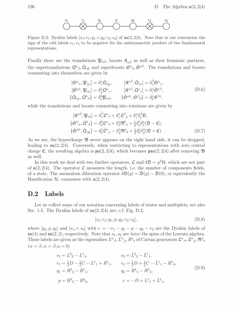
196 D The Algebra u(2, 2|4)
s1 r1 q1 p q2 r2 s2
Figure D.2: Dynkin labels [s1; r1; q1, r, q2; r2; s2] of su(2, 2|4). Note that in our convention thesign of the odd labels r1, r2 to be negative for the antisymmetric product of two fundamentalrepresentations.
Finally there are the translations Pαβ, boosts Kαβ as well as their fermionic partners,
the supertranslations Qaβ, Qαb and superboosts Sα
b, Saβ. The translations and boosts
commuting into themselves are given by
[Sαa,Pβγ] = δαγ Qβa, [Kαβ, Qγc] = δβγS
αc,
[Saα,Pβγ] = δαβQa
γ , [Kαβ,Qcγ ] = δαγ Scβ,
{Qαa,Qbβ} = δbaPαβ, {Saα,Sβ
b} = δabKβα,
(D.6)
while the translations and boosts commuting into rotations are given by
[Kαβ,Pγδ] = δβγLαδ + δαγ Lβ
δ + δαγ δβ
δD,
{Sαa,Q
bβ} = δbaL
αβ + δαβRb
a + 12δbaδ
αβ (D− C),
{Saα, Qβb} = δab Lαβ − δαβRa
b + 12δab δ
αβ(D + C). (D.7)
As we see, the hypercharge B never appears on the right hand side, it can be dropped,leading to su(2, 2|4). Conversely, when restricting to representations with zero centralcharge C, the resulting algebra is pu(2, 2|4), which becomes psu(2, 2|4) after removing B
as well.In this work we deal with two further operators, L and δD = g2H, which are not part
of u(2, 2|4). The operator L measures the length, i.e. the number of components fields,of a state. The anomalous dilatation operator δD(g) = D(g)−D(0), or equivalently theHamiltonian H, commutes with u(2, 2|4).
D.2 Labels
Let us collect some of our notation concerning labels of states and multiplets, see alsoSec. 1.5. The Dynkin labels of su(2, 2|4) are, c.f. Fig. D.2,
[s1; r1; q1, p, q2; r2; s2], (D.8)
where [q1, p, q2] and [s1, r, s2] with r = −r1 − q1 − p − q2 − r2 are the Dynkin labels ofsu(4) and su(2, 2), respectively. Note that s1, s2 are twice the spins of the Lorentz algebra.These labels are given as the eigenvalues Lαβ, L
αβ, R
ab of Cartan generators Lα
β, Lαβ,R
ab
(α = β, α = β, a = b)
s1 = L22 − L1
1, s2 = L22 − L1
1,
r1 = 12D − 1
2C − L1
1 +R11, r2 = 1
2D + 1
2C − L1
1 −R44,
q1 = R22 −R1
1, q2 = R44 −R3
3,
p = R33 −R2
2, r = −D + L11 + L1
1.
(D.9)

D.3 The Quadratic Casimir 197
We also use the notation
(D0, s1, s2; q1, p, q2;B,L) (D.10)
to describe states of the classical theory. The label B is the hypercharge measured by B.The length L corresponds to the number of fields within a state, it is measured by theoperator L which is not part of u(2, 2|4). D0 is the classical dimension and we introduceE as the ‘energy’ or anomalous dimension measured by H = g−2δD. Together they formthe scaling dimension D = D0 + g2E which is measured by D = D0 + g2H. Usually wewill state only the classical dimension D0 to specify a state; the corresponding energyE will be the main result of a our computations. It is useful to know how to translatebetween the dimension D and Dynkin labels r1, r2, r, see (D.9),
r1 = 12D − 1
2C − 1
2p− 3
4q1 − 1
4q2 + 1
2s1,
r2 = 12D + 1
2C − 1
2p− 1
4q1 − 3
4q2 + 1
2s2,
r = −D − 12s1 − 1
2s2,
r = −r1 − q1 − p− q2 − r2D = −1
2s1 + r1 + q1 + p+ q2 + r2 − 1
2s2. (D.11)
D.3 The Quadratic Casimir
The quadratic Casimir of u(2, 2|4) is
J2 = 12D2 + 1
2Lγ
δLδγ + 1
2Lγ
δLδγ − 1
2Rc
dRdc
− 12[Qc
γ,Sγc]− 1
2[Qγc, S
γc]− 12{Pγδ,K
δγ} −BC. (D.12)
In psu(2, 2|4) the last term BC is absent. For highest weight states, which are annihilatedby raising operators J+ (1.53), we can conveniently evaluate J2 by using the standardtrick of turning the anticommutators into commutators. We find
J2 = 14s1(s1 + 2) + 1
4s2(s2 + 2) + 1
2D2 + 2D − BC
− 14q1(q1 + 2)− 1
4q2(q2 + 2)− 1
8(2p+ q1 + q2)
2 − (2p+ q1 + q2). (D.13)
D.4 The Oscillator Representation
Let us explain the use of oscillators for fields and generators in terms of the algebragl(M): We write1
JAB = A†BAA, with A,B = 1, . . . ,M. (D.14)
Using the commutators
[AA,A†B] = δAB, [AA,AB] = [A†
A,A†B] = 0 (D.15)
it is a straightforward exercise to show that the generators J satisfy the gl(M) algebra.
1Strictly speaking, the oscillators A and A† are independent. Only in one of the real forms of gl(M)
they would be related by conjugation.

198 D The Algebra u(2, 2|4)
To construct an oscillator representation for u(2, 2|4), c.f. [93], we will consider two setsof bosonic oscillators (aα, a†
α), (bα,b†α) with α, α = 1, 2 and one set of fermionic oscillator
(ca, c†a) with a = 1, 2, 3, 4. The non-vanishing commutators of oscillators are taken to be
[aα, a†β] = δαβ , [bα,b†
β] = δα
β, {ca, c†b} = δab . (D.16)
We assume that the oscillators AA = (a,b†, c) and A†A = (a†,−b, c†) form a fundamental
and conjugate fundamental multiplet of u(2, 2|4). Then, the bilinears A†AA
B generate thealgebra u(2, 2|4) as described above. By comparing to the matrix form (D.1) we can readoff the generators in su(2) × su(2) × su(4) notation. The canonical forms for rotationgenerators of su(2), su(2) and su(4) are
Lαβ = a†
βaα − 1
2δαβa
†γa
γ,
Lαβ = b†
βbα − 1
2δαβb†γb
γ ,
Rab = c†bc
a − 14δab c
†ccc. (D.17)
Under these the fields (1.78) transform canonically. We write the corresponding threeu(1) charges as
D = 1 + 12a†γa
γ + 12b†γb
γ,
C = 1− 12a†γa
γ + 12b†γb
γ − 12c†cc
c,
B = 12a†γa
γ − 12b†γb
γ . (D.18)
The remaining off-diagonal generators are
Qaα = a†
αca, Sα
a = c†aaα,
Qαa = b†αc
†a, Sαa = bαca,
Pαβ = a†αb
†β, Kαβ = aαbβ . (D.19)
Quite naturally the algebra u(2, 2|4) is realised by the generators (D.17,D.18,D.19).2 Wehave written this in a su(2) × su(2) × su(4) covariant way. In fact one can combine theindices a and α into a superindex and obtain a manifest su(2) × su(2|4) notation. Thegenerators with two lower or two upper indices, P, Q,K, S, together with the remainingcharges complete the u(2, 2|4) algebra.
Instead of one fermionic oscillator (ca, c†a) with a = 1, 2, 3, 4, we can also introducetwo pairs of oscillators (ca, c†a) and (da,d†
a) with a, a = 1, 2. These should be grouped asAA = (a,b†, c,d†) and A†
A = (a†,−b, c†,d) into fundamental representations of u(2, 2|4).Despite the fact that only su(2)4 (or psu(2|2)2 when using superindices) is manifest inthis notation, it has the added benefit that we can define a physical vacuum state |Z〉 by
aα|Z〉 = bα|Z〉 = ca|Z〉 = da|Z〉 = 0. (D.20)
This is the highest weight state of the field multiplet, see Sec. 1.9.
2Note that a shift of B by a constant (−1) does not modify the algebra. Then the 1 in D, C, B can
be absorbed into 1 + 12b
†γb
γ = 12b
γb†γ to yield a canonical form.

D.4 The Oscillator Representation 199
na =
(12D0 + 1
2B − 1
2L− 1
2s1
12D0 + 1
2B − 1
2L+ 1
2s1
), nb =
(12D0 − 1
2B − 1
2L− 1
2s2
12D0 − 1
2B − 1
2L+ 1
2s2,
),
nc =
(12L− 1
2B − 1
2p− 3
4q1 − 1
4q2
12L− 1
2B − 1
2p+ 1
4q1 − 1
4q2
), nd =
(12L+ 1
2B − 1
2p− 1
4q1 − 3
4q2
12L+ 1
2B − 1
2p− 1
4q1 + 1
4q2
),
nc =
12L− 1
2B − 1
2p− 3
4q1 − 1
4q2
12L− 1
2B − 1
2p+ 1
4q1 − 1
4q2
12L− 1
2B + 1
2p+ 1
4q1 − 1
4q2
12L− 1
2B + 1
2p+ 1
4q1 + 3
4q2
.
Table D.2: Oscillator excitation numbers for a state with given charges.
a†1a
2a†2c
1c†1c
2c†2d
†2 d
†1d
2b†2d
1b†1b
2
Figure D.4: Oscillator representation of simple roots.
In this context it is useful to know how to represent a state with a given weight
w = (D0; s1, s2; q1, p, q2;B,L) (D.21)
in terms of excitations of the oscillators. We introduce a multi-particle vacuum operator|Z, L〉 which is the tensor product of L vacua |Z〉. The oscillators a†
p,α,b†p,α, c
†p,a,d
†p,a.
now act on site p, where commutators of two oscillators vanish unless the sites agree.Equivalently, we define the unphysical multi-particle vacuum state |0, L〉. A generic stateis written as
(a†)na(b†)nb(c†)nc(d†)nd|Z, L〉 or (a†)na(b†)nb(c†)nc|0, L〉. (D.22)
By considering the weights of the oscillators as well as the central charge constraint,we find the number of excitations as given in Tab. D.2.3 It is also useful to know howto represent the generators corresponding to the simple roots in terms of creation andannihilation operators, c.f. Fig. D.4.
3The components of the vectors correspond to the numbers of each component of the oscillators.

200

201
Appendix E
Tools for the su(2) Sector
In this appendix we present a basic set of Mathematica routines to deal with su(2)spin chains at higher-loops.
E.1 States
One of the basic objects is a state |. . .〉, in Mathematica it will be represented by thefunction Chain[...], e.g.
Chain[0,0,1,0,1,1,0] = |0, 0, 1, 0, 1, 1, 0〉 = TrZZφZφφZ. (E.1)
This function is undefined and Mathematica will leave it as it stands and not try toevaluate it. For example one can construct linear combinations of states, e.g.
2|0, 0, 1, 1〉+ |0, 1, 0, 1〉 = 2 Chain[0,0,1,1] + Chain[0,1,0,1]. (E.2)
We consider spin chain states only modulo cyclic permutations. The order has to beimplemented manually and we need a routine to shift states into some canonical order
SortChain[X_] := X /. C_Chain :>
Module[{k}, Sort[Table[RotateLeft[C, k], {k, Length[C]}]][[1]]];
This function returns the argument X with all chains ordered. It works as follows: Firstof all, all states C=Chain[...] within X are found. For each C a list of all possiblecyclic permutations is generated and sorted. The first element is taken as the canonicallyordered state and returned.
We can now define a simple operation on states, the parity p which reverses the spinchain and multiplies by (−1)L
ChainParity[X_] := X /. C_Chain :> (-1)^Length[C] SortChain[Reverse[C]];
Conveniently, it shifts the states into a canonical order.
E.2 Interactions
The other basic object is an interaction {. . .} which will be represented by Perm[...]
Perm[1,3,2] = {1, 3, 2}. (E.3)

202 E Tools for the su(2) Sector
We need a representation for the action of permutation symbols {. . .}|. . .〉, this is doneby
ApplyPerm[P_, C_] := P /. P0_Perm :> (C /. C0_Chain -> ApplyPermPC[P0, C0]);
ApplyPermPC[P_Perm, C_Chain] :=
Module[{s}, Sum[PermuteList[C, P, s], {s, Length[C]}]];
The function ApplyPerm assumes P and C are linear combinations of interactions andstates. It distributes the elementary interactions and states and passes on to ApplyPermPC
for an elementary pair. This uses another function PermuteList to apply the permutationto each site s of the spin chain
PermuteList[C_Chain, Perm[], s_] := C;
PermuteList[C_Chain, P_Perm, s_] :=
PermuteList[PermuteElements[C, Last[P] + s], Drop[P, -1], s];
PermuteElements[C_Chain, p_] :=
Module[{p0 = Mod[p, Length[C], 1], p1 = Mod[p + 1, Length[C], 1]},
ReplacePart[ReplacePart[C, C[[p0]], p1], C[[p1]], p0]];
The routine PermuteList recursively works on the permutation symbol P from the rightand uses PermuteElements to perform the pairwise permutations.
E.3 Spectrum
To find the spectrum of an operator, we need to find a complete basis of states onwhich the operator closes. This basis is generated by
GenerateChains[L_, K_] :=
(Chain @@ Join[Array[1 &, K], Array[0 &, L - K]])
// Permutations // SortChain // Union;
The function returns a basis of states of L sites with n excitations. It is then convenientto have a method to evaluate the action of an operator on a basis of states
ActionMatrix[P_, C_] := CoeffList[ApplyPerm[P, C] // SortChain, C];
It returns a matrix that is equivalent to the action of P in the basis C. It requires themulti-purpose function
CoeffList[X_, L_] := Map[Coefficient[X, #] &, L];
which expands a linear expression X over a basis of atoms L.
E.4 An Example
We can now find the energy of states with length L=4 and K=2 excitations. Let us firstconstruct a basis of states
Ops = GenerateChains[4, 2]
> {Chain[0, 0, 1, 1], Chain[0, 1, 0, 1]}
The one-loop Hamiltonian is given by H0 = {} − {1} so let us define
Ham = Perm[] - Perm[1];

E.5 Commutators 203
and act on the above basis
MHam = ActionMatrix[Ham, Ops]
> {{2, -4}, {-2, 4}}
The eigenvalues are
Eigenvalues[MHam]
> {0, 6}
Eigenvectors[MHam]
> {{2, 1}, {-1, 1}}
where the energy E = 0 belongs to the state 2|0, 0, 1, 1〉 + |0, 1, 0, 1〉 and E = 6 to theKonishi state −|0, 0, 1, 1〉+ |0, 1, 0, 1〉.
E.5 Commutators
For investigations of integrability we require methods to compute commutators ofinteractions abstractly. This is a straightforward implementation of the commutator ofpermutation symbols
CommutePerm[X_, Y_] :=
X /. P1_Perm :> (Y /. P2_Perm -> CommutePerm12[P1, P2]) // SimplifyPerm;
CommutePerm12[Perm[X___], Perm[Y___]] :=
Module[{MX = Max[X, 0] + 1, MY = Max[Y, 0] + 1, k},
Sum[Perm @@ Join[{X} + k - 1, {Y} + MX - 1] -
Perm @@ Join[{Y} + MX - 1, {X} + k - 1], {k, MX + MY - 1}]];
As above, CommutePerm distributes linear combinations and calls CommutePerm12 for el-ementary commutators. Finally, we should simplify the permutation symbols using therules in Sec. 6.2.1
SimplifyPerm[YY_] := (YY //.
{Perm[X__ /; Min[X] != 1] :> Perm @@ ({X} - Min[X] + 1),
Perm[X___, y_, y_, Z___] -> Perm[X, Z],
Perm[X___, y_, z_, y_, W___]
/; (z == y + 1) || (z == y - 1)
-> Perm[X, W] - Perm[X, y, W] - Perm[X, z, W]
+ Perm[X, y, z, W] + Perm[X, z, y, W],
Perm[X___, y_, z_, W___]
/; z < y - 1
-> Perm[X, z, y, W],
Perm[X___, y_, z_, W__, y_, V___]
/; (z == y - 1) && (! MemberQ[{W}, k_ /; k > y - 2])
-> Perm[X, y, z, y, W, V],
Perm[X___, y_, W__, z_, y_, V___]
/; (z == y + 1) && (! MemberQ[{W}, k_ /; k < y + 2])
-> Perm[X, W, y, z, y, V]}) // Expand;
For the construction of higher-loop interactions, one can write functions to construct abasis of interaction symbols for a given loop order and to solve commutators for unknowncoefficients. As the construction still requires a sufficient amount of manual work, we willnot present these here.

204

205
Appendix F
The Harmonic Action
The Hamiltonian density H12 is given by an psu(2, 2|4) invariant function acting ontwo sites,
H12 = 2h(J12). (F.1)
We will now describe explicitly how H12 acts on a state of two fields in the oscillatorrepresentation, see Sec. 1.9.
F.1 Generic Invariant Action
We will investigate the action of a generic function f(J12) on two oscillator sites. Letus introduce a collective oscillator A†
A = (a†α,b
†α, c
†a,d
†a). A general state in VF × VF can
be written as|p1, . . . , pn;A〉 = A†
p1,A1. . .A†
pn,An|ZZ〉, (F.2)
subject to the central charge constraints C1|X〉 = C2|X〉 = 0. The label pk = 1, 2determines the site on which the k-th oscillator acts. The action of psu(2, 2|4) conservesthe number of each type of oscillator; it can however move oscillators between both sites.Therefore the action of f(J12) is
f(J12) |p1, . . . , pn;A〉 =∑
p′1,...p′n
cp,p′,A δC1,0δC2,0 |p′1, . . . , p′n;A〉 (F.3)
with some coefficients cs,s′,A. The sums go over the sites 1, 2 and δC1,0, δC2,0 project tostates where the central charge at each site is zero. In view of the fact that oscillatorsrepresent indices of fields, see (1.79), a generic invariant operator f(J12) acts on two fieldsby moving indices between them.
F.2 The Harmonic Action
The action of the harmonic numbers within the Hamiltonian density H12 = 2h(J12)turns out to be particularly simple. It does not depend on the types of oscillators Ak, butonly on the number of oscillators which change the site
H12|s1, . . . , sn;A〉 =∑
s′1,...s′n
cn,n12,n21δC1,0δC2,0 |s′1, . . . , s′n;A〉. (F.4)

206 F The Harmonic Action
Here n12, n21 count the number of oscillators hopping from site 1 to 2 or vice versa. Thecoefficients cn,n12,n21
are given by
cn,n12,n21= (−1)1+n12n21
Γ(
12(n12 + n21)
)Γ(1 + 1
2(n− n12 − n21)
)
Γ(1 + 1
2n) . (F.5)
In the special case of no oscillator hopping we find
cn,0,0 = h(12n), (F.6)
which can be regarded as a regularisation of (F.5). We will refer to this action givenby (F.4,F.5,F.6) as the ‘harmonic action’. Interestingly, we find that the action of theHamiltonian density using the su(4|2)× su(2) invariant vacuum (c.f. Sec. 1.9) is given byexactly the same expressions.
F.3 Proof
To prove that H12 is given by (F.4,F.5,F.6) it suffices to show
[J12,H12] = 0, H12 Vj = 2h(j)Vj. (F.7)
The invariance of H12 under the subalgebra psu(2|2)× psu(2|2) is straightforward: Thesegenerators only change the types of oscillators, whereas the harmonic action does notdepend on that. In contrast, the remaining generators change the number of oscillatorsby two.
Consider a generator which increases the number of oscillators by two, e.g. P12,αβ , andact with H12P12,αβ on a generic state. First we apply P
P12,αβ |p1, . . . , pn;A〉 = |1, 1, p1, . . . , pn;A′〉+ |2, 2, p1, . . . , pn;A
′〉, (F.8)
and get a state with two new oscillators, A′ = (α, β, A). We apply the Hamiltoniandensity (F.4) to this state and get eight terms (to be summed over all p′k). In two of theseterms, both new oscillators end up at site 1
cn+2,n12,n21|1, 1, p′1, . . . , p′n;A′〉+ cn+2,n12,n21+2|1, 1, p′1, . . . , p′n;A′〉. (F.9)
Here, n12, n21 refer only to the hopping of the old oscillators. Both coefficients can becombined using (F.5)
cn+2,n12,n21+ cn+2,n12,n21+2 = cn,n12,n21
. (F.10)
We pull the additional two oscillators out of the state and get
(cn+2,n12,n21
+ cn+2,n12,n21+2
)|1, 1, p′1, . . . , p′n;A′〉 = P1,αβ cn,n12,n21
|p′1, . . . , p′n;A〉. (F.11)
Summing over all p′k therefore yields P1,αβH12|p1, . . . , pn;A〉. If both new oscillators endup at site 2 we get an equivalent result. It remains to be shown that the other four termscancel. Two of these are
cn+2,n12,n21+1|1, 2, p′1, . . . , p′n;A′〉+ cn+2,n12+1,n21|1, 2, p′1, . . . , p′n;A′〉. (F.12)

F.4 An Example 207
The absolute values in (F.5) match for cn+2,n12,n21+1 and cn+2,n12+1,n21and we sum up the
signs
(−1)1+n12n21+n12 + (−1)1+n12n21+n21 = (−1)1+n12n21((−1)n12 + (−1)n21
). (F.13)
Now, oscillators always hop in pairs due to the central charge constraint. One of the newoscillators has changed the site, so the number of old oscillators changing site must beodd. The above two signs must be opposite and cancel in the sum. The same is truefor the remaining two terms. This concludes the proof for [P12,αβ ,H12] = 0. The prooffor the other generators which increase the number of oscillators is equivalent. To proveinvariance under the remaining generators, we note that these remove two oscillators fromone of the two sites. Assume it will remove the first two oscillators from a state (for eachtwo oscillators that are removed, the argument will be the same). Now, the argument isessentially the same as the proof for P12,αβ read in the opposite direction.
To prove that the eigenvalues of H12 are given by 2h(j), we act on a state |j〉 of Vjwithin the bosonic su(1, 1) subsector, c.f. Sec. 3.4
|j〉 =
j∑
k=0
(−1)kj!
k!(j − k)! |k, j − k〉 (F.14)
with a single spin given by
|k〉 =1
k!(a†
2)k(b†
2)k |Z〉. (F.15)
The state |j〉 has a definite spin and is therefore an eigenstate of H12. We can choose tocalculate only the coefficient of |j, 0〉 in H12|j〉. It is given by (see Sec. 3.2.6)
h(j) +
j∑
k=1
(−1)1+kj!
k k!(j − k)! = 2h(j), (F.16)
which proves that H12 = 2h(J12). This concludes the proof of (F.7).
F.4 An Example
We will now determine the planar anomalous dimensions of some states with weight(2; 0, 0; 0, 0, 0; 0, 2) to demonstrate how to apply the above Hamiltonian. Using Tab. D.2we find that we have to excite each of the four oscillators c,d once. There must be anequal number of c and d oscillators on each site due to the central charge constraint andthe three distinct configurations are
|1212〉 = c†1,1c†2,2d
†1,1d
†2,2|ZZ〉,
|1221〉 = c†1,1c†2,2d
†2,1d
†1,2|ZZ〉,
|1111〉 = c†1,1c†1,2d
†1,1d
†1,2|ZZ〉. (F.17)
Let us now act with H12 on these states, we find
H12|1212〉 = c4,0,0|1212〉+ c4,0,2|1111〉+ c4,2,0|2222〉+ c4,1,1|2112〉+ c4,1,1|1221〉+ c4,2,2|2121〉
= 32|1212〉 − 1
2|1111〉 − 1
2|2222〉+ 1
2|2112〉+ 1
2|1221〉 − 1
2|2121〉
= |1212〉+ |1221〉 − |1111〉 (F.18)

208 F The Harmonic Action
using (F.4,F.5,F.6) and cyclicity of the trace. Evaluating the Hamiltonian for the remain-ing two states |1212〉 and |1221〉 we find the energy matrix
H =
2 2 −22 2 −2−2 −2 2
. (F.19)
the factor of 2 is due to H = H12 +H21. One eigenstate is
|K〉 = |1212〉+ |1221〉 − |1111〉. (F.20)
with energy E = 6; it is clearly part of the Konishi multiplet. The other two, |1212〉 +|1111〉 and |1221〉 + |1111〉, have vanishing energy and belong to the half-BPS currentmultiplet.

a
Acknowledgements
Here, I would like to express my gratitude to my advisor, Matthias Staudacher, for allthe support, encouragement, advice, time, stimulating discussions, disputes, chocolatesand fantastic collaboration throughout the last two years. Without his keen sense ofinteresting physical problems, this work would not be the same. Also, I thank him forbeing the sociable person he is, this made my time in Potsdam as well as on joint travelsboth exciting and pleasant.
I have also benefitted very much from everyday discussions with Gleb Arutyunov,Charlotte Kristjansen and Jan Plefka and thank them for sharing their knowledge onvarious aspects of physics. Especially, I will never forget the afternoons spent in Matthias’soffice drinking tea and discussing the latest discoveries with each other.
I am grateful to Massimo Bianchi, Virginia Dippel, Sergey Frolov, Charlotte Krist-jansen, Joe Minahan, Francisco Morales, Jan Plefka, Henning Samtleben, Gordon Se-menoff, Matthias Staudacher, Arkady Tseytlin and Kostya Zarembo for the fruitful col-laboration on the projects on which this thesis is based in part.
I thank Virginia Dippel, Markus Possel, Matthias Staudacher and Arkady Tseytlin forproof-reading the manuscript and suggesting valuable improvements to make your readingof this text more enjoyable. I also thank the referees of the dissertation, Curtis Callan,Hermann Nicolai and Jan Plefka, for their time. Again, thanks are due to Matthias forall the help while preparing earlier articles.
For interesting discussions of physics and otherwise, it is a pleasure to thank VladimirBazhanov, Andrei Belitsky, David Berenstein, Vladimir Braun, Chong-Sun Chu, NeilConstable, Luise Dolan, Thomas Fischbacher, Dan Freedman, Jaume Gomis, Alexan-der Gorsky, Christine Gottschalkson, Petra Gutjahr, Paul Howe, Hikaru Kawai, VolodyaKazakov, Nakwoo Kim, Axel Kleinschmidt, Thomas Klose, Gregory Korchemsky, DavidKosower, Stefano Kovacs, Juan Maldacena, Shiraz Minwalla, Chiara Nappi, Ari Pankie-wicz, Christina Pappa, Kasper Peeters, Markus Possel, Thomas Quella, Rodolfo Russo,Anton Ryzhov, Kazuhiro Sakai, Dierk Schleicher, John Schwarz, Didina Serban, CorneliuSochichiu, Emery Sokatchev, Marcus Spradlin, Bogdan Stefanski, Ian Swanson, Diana Va-man, Herman Verlinde, Edward Witten, Marija Zamaklar and fellow physicists I have metat seminars, schools and conferences as well as everybody I have unfortunately missed.
I would like to thank my office-mates, colleagues and members of staff at the Institutefor the pleasant, inspiring atmosphere and for making my work so enjoyable. In particular,I acknowledge the prompt help by the computer support when my laptop went to thehappy hunting grounds after four and a half years of loyal service around the world.
Ich mochte mich ganz herzlich bei Anna, Thomas, Maissi, Miriam und meinen Freun-den fur ihre fortwahrende Unterstutzung bedanken, ohne die diese Arbeit in der jetzigenForm nicht moglich gewesen ware.

b Acknowledgements
Schließlich bedanke ich mich bei der Studienstiftung des deutschen Volkes fur dieUnterstutzung durch ein Promotionsforderungsstipendium, sowie auch bei meinem Ver-trauensdozenten Prof. Dr. Harald Uhlig und Mit-Stiftis fur ihr Engagement. Die Som-merakademie 2003 in St. Johann hat sehr zur Erweiterung meiner Horizonte beigetra-gen. Ebenso hoffe ich auf dem nun folgenden Sprachkurs in Amboise nicht nur meineFranzosischkenntnisse verbessern zu konnen, sondern mich auch von den Strapazen desAnfertigens dieser Arbeit zu erholen.
Thank You!

c
References
[1] G. ’t Hooft, “A Planar Diagram Theory for Strong Interactions”,Nucl. Phys. B72, 461 (1974).
[2] F. Gliozzi, J. Scherk and D. I. Olive, “Supersymmetry, Supergravity theories and thedual spinor model”, Nucl. Phys. B122, 253 (1977). • L. Brink, J. H. Schwarz andJ. Scherk, “Supersymmetric Yang-Mills Theories”, Nucl. Phys. B121, 77 (1977).
[3] M. F. Sohnius and P. C. West, “Conformal invariance in N = 4 SupersymmetricYang-Mills Theory”, Phys. Lett. B100, 245 (1981). • S. Mandelstam, “Light ConeSuperspace and the Ultraviolet Finiteness of the N = 4 Model”,Nucl. Phys. B213, 149 (1983). • P. S. Howe, K. S. Stelle and P. K. Townsend,“Miraculous ultraviolet cancellations in supersymmetry made manifest”,Nucl. Phys. B236, 125 (1984). • L. Brink, O. Lindgren and B. E. W. Nilsson, “N = 4Yang-Mills theory on the light cone”, Nucl. Phys. B212, 401 (1983).
[4] J. M. Maldacena, “The large N limit of superconformal field theories and supergravity”,Adv. Theor. Math. Phys. 2, 231 (1998), hep-th/9711200.
[5] S. S. Gubser, I. R. Klebanov and A. M. Polyakov, “Gauge theory correlators fromnon-critical string theory”, Phys. Lett. B428, 105 (1998), hep-th/9802109.
[6] E. Witten, “Anti-de Sitter space and holography”, Adv. Theor. Math. Phys. 2, 253 (1998),hep-th/9802150.
[7] O. Aharony, S. S. Gubser, J. M. Maldacena, H. Ooguri and Y. Oz, “Large N fieldtheories, string theory and gravity”, Phys. Rept. 323, 183 (2000), hep-th/9905111. •E. D’Hoker and D. Z. Freedman, “Supersymmetric gauge theories and the AdS/CFTcorrespondence”, hep-th/0201253, in: “Strings, branes and extra dimensions”,Proceedings of TASI 2001, Boulder, Colorado, USA, 4-29 June 2001, ed.: S. S. Gubserand J. D. Lykken, World Scientific (2004), Singapore.
[8] V. K. Dobrev and V. B. Petkova, “All positive energy unitary irreducible representationsof extended conformal supersymmetry”, Phys. Lett. B162, 127 (1985).
[9] L. Andrianopoli and S. Ferrara, “Short and long SU(2,2/4) multiplets in the AdS/CFTcorrespondence”, Lett. Math. Phys. 48, 145 (1999), hep-th/9812067.
[10] L. Andrianopoli, S. Ferrara, E. Sokatchev and B. Zupnik, “Shortening of primaryoperators in N-extended SCFT4 and harmonic-superspace analyticity”,Adv. Theor. Math. Phys. 3, 1149 (1999), hep-th/9912007.
[11] S.-M. Lee, S. Minwalla, M. Rangamani and N. Seiberg, “Three-point functions of chiraloperators in D = 4, N = 4 SYM at large N”, Adv. Theor. Math. Phys. 2, 697 (1998),hep-th/9806074.

d References
[12] G. Arutyunov, S. Frolov and A. C. Petkou, “Operator product expansion of the lowestweight CPOs in N = 4 SYM4 at strong coupling”, Nucl. Phys. B586, 547 (2000),hep-th/0005182.
[13] M. Bianchi, M. B. Green, S. Kovacs and G. Rossi, “Instantons in supersymmetricYang-Mills and D-instantons in IIB superstring theory”, JHEP 9808, 013 (1998),hep-th/9807033.
[14] D. Berenstein, J. M. Maldacena and H. Nastase, “Strings in flat space and pp wavesfrom N = 4 Super Yang Mills”, JHEP 0204, 013 (2002), hep-th/0202021.
[15] M. Blau, J. Figueroa-O’Farrill, C. Hull and G. Papadopoulos, “A new maximallysupersymmetric background of IIB superstring theory”, JHEP 0201, 047 (2002),hep-th/0110242. • M. Blau, J. Figueroa-O’Farrill, C. Hull and G. Papadopoulos,“Penrose limits and maximal supersymmetry”, Class. Quant. Grav. 19, L87 (2002),hep-th/0201081.
[16] R. R. Metsaev, “Type IIB Green-Schwarz superstring in plane wave Ramond-Ramondbackground”, Nucl. Phys. B625, 70 (2002), hep-th/0112044. • R. R. Metsaev andA. A. Tseytlin, “Exactly solvable model of superstring in plane wave Ramond-Ramondbackground”, Phys. Rev. D65, 126004 (2002), hep-th/0202109.
[17] A. Pankiewicz, “Strings in plane wave backgrounds”, Fortsch. Phys. 51, 1139 (2003),hep-th/0307027. • J. C. Plefka, “Lectures on the plane-wave string / gauge theoryduality”, Fortsch. Phys. 52, 264 (2004), hep-th/0307101. • C. Kristjansen, “Quantummechanics, random matrices and BMN gauge theory”,Acta Phys. Polon. B34, 4949 (2003), hep-th/0307204. • D. Sadri andM. M. Sheikh-Jabbari, “The plane-wave / super Yang-Mills duality”,Rev. Mod. Phys. 76, 853 (2004), hep-th/0310119. • R. Russo and A. Tanzini, “Theduality between IIB string theory on pp-wave and N = 4 SYM: A status report”,Class. Quant. Grav. 21, S1265 (2004), hep-th/0401155.
[18] C. Kristjansen, J. Plefka, G. W. Semenoff and M. Staudacher, “A new double-scalinglimit of N = 4 super Yang-Mills theory and PP-wave strings”,Nucl. Phys. B643, 3 (2002), hep-th/0205033.
[19] N. R. Constable, D. Z. Freedman, M. Headrick, S. Minwalla, L. Motl, A. Postnikov andW. Skiba, “PP-wave string interactions from perturbative Yang-Mills theory”,JHEP 0207, 017 (2002), hep-th/0205089.
[20] M. Spradlin and A. Volovich, “Superstring interactions in a pp-wave background”,Phys. Rev. D66, 086004 (2002), hep-th/0204146.
[21] N. Beisert, C. Kristjansen, J. Plefka, G. W. Semenoff and M. Staudacher, “BMNcorrelators and operator mixing in N = 4 super Yang-Mills theory”,Nucl. Phys. B650, 125 (2003), hep-th/0208178.
[22] N. R. Constable, D. Z. Freedman, M. Headrick and S. Minwalla, “Operator mixing andthe BMN correspondence”, JHEP 0210, 068 (2002), hep-th/0209002.
[23] R. Roiban, M. Spradlin and A. Volovich, “On light-cone SFT contact terms in a planewave”, JHEP 0310, 055 (2003), hep-th/0211220.
[24] J. Pearson, M. Spradlin, D. Vaman, H. Verlinde and A. Volovich, “Tracing the String:BMN correspondence at Finite J2/N”, JHEP 0305, 022 (2003), hep-th/0210102.
[25] D. J. Gross, A. Mikhailov and R. Roiban, “Operators with large R charge in N = 4Yang-Mills theory”, Annals Phys. 301, 31 (2002), hep-th/0205066.
References e
[26] A. Parnachev and A. V. Ryzhov, “Strings in the near plane wave background andAdS/CFT”, JHEP 0210, 066 (2002), hep-th/0208010.
[27] N. Beisert, “BMN Operators and Superconformal Symmetry”,Nucl. Phys. B659, 79 (2003), hep-th/0211032.
[28] T. Klose, “Conformal Dimensions of Two-Derivative BMN Operators”,JHEP 0303, 012 (2003), hep-th/0301150.
[29] B. Eynard and C. Kristjansen, “BMN correlators by loop equations”,JHEP 0210, 027 (2002), hep-th/0209244.
[30] U. Gursoy, “Vector operators in the BMN correspondence”, JHEP 0307, 048 (2003),hep-th/0208041. • U. Gursoy, “Predictions for pp-wave string amplitudes fromperturbative SYM”, JHEP 0310, 027 (2003), hep-th/0212118.
[31] E. D’Hoker, D. Z. Freedman and W. Skiba, “Field theory tests for correlators in theAdS/CFT correspondence”, Phys. Rev. D59, 045008 (1999), hep-th/9807098.
[32] S. Penati, A. Santambrogio and D. Zanon, “Two-point functions of chiral operators inN = 4 SYM at order g4”, JHEP 9912, 006 (1999), hep-th/9910197. • S. Penati,A. Santambrogio and D. Zanon, “More on correlators and contact terms in N = 4 SYMat order g4”, Nucl. Phys. B593, 651 (2001), hep-th/0005223.
[33] S. Penati and A. Santambrogio, “Superspace approach to anomalous dimensions inN = 4 SYM”, Nucl. Phys. B614, 367 (2001), hep-th/0107071.
[34] A. V. Ryzhov, “Quarter BPS operators in N = 4 SYM”, JHEP 0111, 046 (2001),hep-th/0109064.
[35] N. Beisert, C. Kristjansen, J. Plefka and M. Staudacher, “BMN gauge theory as aquantum mechanical system”, Phys. Lett. B558, 229 (2003), hep-th/0212269.
[36] D. J. Gross, A. Mikhailov and R. Roiban, “A calculation of the plane wave stringHamiltonian from N = 4 super-Yang-Mills theory”, JHEP 0305, 025 (2003),hep-th/0208231.
[37] R. A. Janik, “BMN operators and string field theory”, Phys. Lett. B549, 237 (2002),hep-th/0209263.
[38] N. Beisert, C. Kristjansen and M. Staudacher, “The dilatation operator of N = 4conformal super Yang-Mills theory”, Nucl. Phys. B664, 131 (2003), hep-th/0303060.
[39] D. Anselmi, M. T. Grisaru and A. Johansen, “A Critical Behaviour of AnomalousCurrents, Electric-Magnetic Universality and CFT4”, Nucl. Phys. B491, 221 (1997),hep-th/9601023.
[40] D. Anselmi, “The N = 4 quantum conformal algebra”, Nucl. Phys. B541, 369 (1999),hep-th/9809192.
[41] M. Bianchi, S. Kovacs, G. Rossi and Y. S. Stanev, “On the logarithmic behavior inN = 4 SYM theory”, JHEP 9908, 020 (1999), hep-th/9906188.
[42] M. Bianchi, S. Kovacs, G. Rossi and Y. S. Stanev, “Anomalous dimensions in N = 4SYM theory at order g4”, Nucl. Phys. B584, 216 (2000), hep-th/0003203. •G. Arutyunov, B. Eden, A. C. Petkou and E. Sokatchev, “Exceptionalnon-renormalization properties and OPE analysis of chiral four-point functions inN = 4 SYM4”, Nucl. Phys. B620, 380 (2002), hep-th/0103230.

f References
[43] A. V. Kotikov and L. N. Lipatov, “NLO corrections to the BFKL equation in QCD andin supersymmetric gauge theories”, Nucl. Phys. B582, 19 (2000), hep-ph/0004008. •A. V. Kotikov and L. N. Lipatov, “DGLAP and BFKL evolution equations in the N = 4supersymmetric gauge theory”, hep-ph/0112346.
[44] F. A. Dolan and H. Osborn, “Superconformal symmetry, correlation functions and theoperator product expansion”, Nucl. Phys. B629, 3 (2002), hep-th/0112251.
[45] M. Bianchi, B. Eden, G. Rossi and Y. S. Stanev, “On operator mixing in N = 4 SYM”,Nucl. Phys. B646, 69 (2002), hep-th/0205321.
[46] G. Arutyunov, S. Penati, A. C. Petkou, A. Santambrogio and E. Sokatchev,“Non-protected operators in N = 4 SYM and multiparticle states of AdS(5) SUGRA”,Nucl. Phys. B643, 49 (2002), hep-th/0206020.
[47] M. Spradlin and A. Volovich, “Note on plane wave quantum mechanics”,Phys. Lett. B565, 253 (2003), hep-th/0303220.
[48] J. A. Minahan and K. Zarembo, “The Bethe-ansatz for N = 4 super Yang-Mills”,JHEP 0303, 013 (2003), hep-th/0212208.
[49] C.-S. Chu, V. V. Khoze and G. Travaglini, “BMN operators with vector impurities, Z2
symmetry and pp-waves”, JHEP 0306, 050 (2003), hep-th/0303107. • G. Georgiou andG. Travaglini, “Fermion BMN operators, the dilatation operator of N = 4 SYM, andpp-wave string interactions”, JHEP 0404, 001 (2004), hep-th/0403188.
[50] N. Beisert, “The Complete One-Loop Dilatation Operator of N = 4 Super Yang-MillsTheory”, Nucl. Phys. B676, 3 (2004), hep-th/0307015.
[51] N. Beisert, “The su(2/3) dynamic spin chain”, Nucl. Phys. B682, 487 (2004),hep-th/0310252.
[52] L. N. Lipatov, “High-energy asymptotics of multicolor QCD and exactly solvable latticemodels”, JETP Lett. 59, 596 (1994), hep-th/9311037.
[53] L. D. Faddeev and G. P. Korchemsky, “High-energy QCD as a completely integrablemodel”, Phys. Lett. B342, 311 (1995), hep-th/9404173.
[54] V. M. Braun, S. E. Derkachov and A. N. Manashov, “Integrability of three-particleevolution equations in QCD”, Phys. Rev. Lett. 81, 2020 (1998), hep-ph/9805225. •A. V. Belitsky, “Fine structure of spectrum of twist-three operators in QCD”,Phys. Lett. B453, 59 (1999), hep-ph/9902361. • V. M. Braun, S. E. Derkachov,G. P. Korchemsky and A. N. Manashov, “Baryon distribution amplitudes in QCD”,Nucl. Phys. B553, 355 (1999), hep-ph/9902375. • A. V. Belitsky, “Integrability andWKB solution of twist-three evolution equations”, Nucl. Phys. B558, 259 (1999),hep-ph/9903512. • A. V. Belitsky, “Renormalization of twist-three operators andintegrable lattice models”, Nucl. Phys. B574, 407 (2000), hep-ph/9907420. •S. E. Derkachov, G. P. Korchemsky and A. N. Manashov, “Evolution equations for quarkgluon distributions in multi-color QCD and open spin chains”,Nucl. Phys. B566, 203 (2000), hep-ph/9909539. • A. V. Belitsky, A. S. Gorsky andG. P. Korchemsky, “Gauge/string duality for QCD conformal operators”,Nucl. Phys. B667, 3 (2003), hep-th/0304028. • G. Ferretti, R. Heise and K. Zarembo,“New Integrable Structures in Large-N QCD”, Phys. Rev. D70, 074024 (2004),hep-th/0404187. • M. Kirch and A. N. Manashov, “Noncompact SL(2,R) spin chain”,JHEP 0406, 035 (2004), hep-th/0405030.
[55] A. V. Belitsky, V. M. Braun, A. S. Gorsky and G. P. Korchemsky, “Integrability in QCDand beyond”, Int. J. Mod. Phys. A19, 4715 (2004), hep-th/0407232.

References g
[56] C. G. Callan, Jr., “Broken scale invariance in scalar field theory”,Phys. Rev. D2, 1541 (1970). • K. Symanzik, “Small distance behavior in field theory andpower counting”, Commun. Math. Phys. 18, 227 (1970).
[57] A. V. Kotikov and L. N. Lipatov, “DGLAP and BFKL equations in the N = 4supersymmetric gauge theory”, Nucl. Phys. B661, 19 (2003), hep-ph/0208220. •A. V. Kotikov, L. N. Lipatov and V. N. Velizhanin, “Anomalous dimensions of Wilsonoperators in N = 4 SYM theory”, Phys. Lett. B557, 114 (2003), hep-ph/0301021.
[58] N. Beisert and M. Staudacher, “The N = 4 SYM Integrable Super Spin Chain”,Nucl. Phys. B670, 439 (2003), hep-th/0307042.
[59] L. D. Faddeev, “How Algebraic Bethe Ansatz works for integrable model”,hep-th/9605187, in: “Relativistic gravitation and gravitational radiation”, Proceedingsof Proceedings of the Les Houches School of Physics, France, 26 Sep-6 Oct, 1995, ed.:J.-A. Marck and J.-P. Lasota, Cambridge University Press (1997), Cambridge.
[60] N. Beisert, J. A. Minahan, M. Staudacher and K. Zarembo, “Stringing Spins andSpinning Strings”, JHEP 0309, 010 (2003), hep-th/0306139.
[61] S. S. Gubser, I. R. Klebanov and A. M. Polyakov, “A semi-classical limit of thegauge/string correspondence”, Nucl. Phys. B636, 99 (2002), hep-th/0204051.
[62] S. Frolov and A. A. Tseytlin, “Semiclassical quantization of rotating superstring inAdS5 × S5”, JHEP 0206, 007 (2002), hep-th/0204226.
[63] S. Frolov and A. A. Tseytlin, “Quantizing three-spin string solution in AdS5 × S5”,JHEP 0307, 016 (2003), hep-th/0306130.
[64] S. Frolov and A. A. Tseytlin, “Rotating string solutions: AdS/CFT duality innon-supersymmetric sectors”, Phys. Lett. B570, 96 (2003), hep-th/0306143.
[65] S. Frolov and A. A. Tseytlin, “Multi-spin string solutions in AdS5 × S5”,Nucl. Phys. B668, 77 (2003), hep-th/0304255.
[66] N. Beisert, S. Frolov, M. Staudacher and A. A. Tseytlin, “Precision Spectroscopy ofAdS/CFT”, JHEP 0310, 037 (2003), hep-th/0308117.
[67] G. Arutyunov, S. Frolov, J. Russo and A. A. Tseytlin, “Spinning strings in AdS5 × S5
and integrable systems”, Nucl. Phys. B671, 3 (2003), hep-th/0307191. • A. Khan andA. L. Larsen, “Spinning pulsating string solitons in AdS5 × S5”,Phys. Rev. D69, 026001 (2004), hep-th/0310019. • J. Engquist, J. A. Minahan andK. Zarembo, “Yang-Mills Duals for Semiclassical Strings”, JHEP 0311, 063 (2003),hep-th/0310188. • G. Arutyunov, J. Russo and A. A. Tseytlin, “Spinning strings inAdS5 × S5: New integrable system relations”, Phys. Rev. D69, 086009 (2004),hep-th/0311004. • A. L. Larsen and A. Khan, “Novel explicit multi spin string solitonsin AdS5”, Nucl. Phys. B686, 75 (2004), hep-th/0312184. • C. Kristjansen, “Three-spinstrings on AdS5 × S5 from N = 4 SYM”, Phys. Lett. B586, 106 (2004),hep-th/0402033. • S. Ryang, “Folded three-spin string solutions in AdS5 × S5”,JHEP 0404, 053 (2004), hep-th/0403180. • M. Lubcke and K. Zarembo, “Finite-sizecorrections to anomalous dimensions in N = 4 SYM theory”, JHEP 0405, 049 (2004),hep-th/0405055. • M. Smedback, “Pulsating strings on AdS5 × S5”,JHEP 0407, 004 (2004), hep-th/0405102. • L. Freyhult, “Bethe ansatz and fluctuationsin SU(3) Yang-Mills operators”, JHEP 0406, 010 (2004), hep-th/0405167. •C. Kristjansen and T. Mansson, “The circular, elliptic three-spin string from the SU(3)spin chain”, Phys. Lett. B596, 265 (2004), hep-th/0406176.

h References
[68] G. Arutyunov and M. Staudacher, “Matching Higher Conserved Charges for Strings andSpins”, JHEP 0403, 004 (2004), hep-th/0310182.
[69] J. Engquist, “Higher conserved charges and integrability for spinning strings inAdS5 × S5”, JHEP 0404, 002 (2004), hep-th/0402092.
[70] G. Arutyunov and M. Staudacher, “Two-loop commuting charges and the string/gaugeduality”, hep-th/0403077, in: “Lie theory and its applications in physics v”,Proceedings of the Fifth International Workshop, Varna, Bulgaria, 16-22 June 2003, ed.:H.-D. Doebner and V. K. Dobrev, World Scientific (2004), Singapore.
[71] M. Kruczenski, “Spin chains and string theory”, Phys. Rev. Lett. 93, 161602 (2004),hep-th/0311203.
[72] M. Kruczenski, A. V. Ryzhov and A. A. Tseytlin, “Large spin limit of AdS5 × S5 stringtheory and low energy expansion of ferromagnetic spin chains”,Nucl. Phys. B692, 3 (2004), hep-th/0403120.
[73] H. Dimov and R. C. Rashkov, “A note on spin chain/string duality”,Int. J. Mod. Phys. A20, 4337 (2005), hep-th/0403121. • R. Hernandez and E. Lopez,“The SU(3) spin chain sigma model and string theory”, JHEP 0404, 052 (2004),hep-th/0403139. • B. Stefanski, Jr. and A. A. Tseytlin, “Large spin limits of AdS/CFTand generalized Landau-Lifshitz equations”, JHEP 0405, 042 (2004), hep-th/0404133. •M. Kruczenski and A. A. Tseytlin, “Semiclassical relativistic strings in S5 and longcoherent operators in N = 4 SYM theory”, JHEP 0409, 038 (2004), hep-th/0406189. •A. A. Tseytlin, “Semiclassical strings in AdS5 × S5 and scalar operators in N = 4 SYMtheory”, Comptes Rendus Physique 5, 1049 (2004), hep-th/0407218.
[74] D. Mateos, T. Mateos and P. K. Townsend, “Supersymmetry of tensionless rotatingstrings in AdS5 × S5, and nearly-BPS operators”, JHEP 0312, 017 (2003),hep-th/0309114. • A. Mikhailov, “Speeding strings”, JHEP 0312, 058 (2003),hep-th/0311019. • A. Mikhailov, “Slow evolution of nearly-degenerate extremalsurfaces”, J. Geom. Phys. 54, 228 (2005), hep-th/0402067. • A. Mikhailov,“Supersymmetric null-surfaces”, JHEP 0409, 068 (2004), hep-th/0404173.
[75] V. A. Kazakov, A. Marshakov, J. A. Minahan and K. Zarembo, “Classical/quantumintegrability in AdS/CFT”, JHEP 0405, 024 (2004), hep-th/0402207.
[76] A. A. Tseytlin, “Spinning strings and AdS/CFT duality”, hep-th/0311139, in: “Fromfields to stings: Circumnavigating theoretical physics”, Ian Kogan Memorial Volume, ed.:M. Shifman, A. Vainshtein and J. Wheater, World Scientific (2005), Singapore.
[77] F. D. M. Haldane, “Exact Jastrow-Gutzwiller resonating valence bond ground state of thespin 1/2 antiferromagnetic Heisenberg chain with 1/r2 exchange”,Phys. Rev. Lett. 60, 635 (1988). • B. S. Shastry, “Exact solution of an S = 1/2 Heisenbergantiferromagnetic chain with long ranged interactions”, Phys. Rev. Lett. 60, 639 (1988).
[78] V. I. Inozemtsev, “On the connection between the one-dimensional s = 1/2 Heisenbergchain and Haldane Shastry model”, J. Stat. Phys. 59, 1143 (1990). • V. I. Inozemtsev,“Integrable Heisenberg-van Vleck chains with variable range exchange”,Phys. Part. Nucl. 34, 166 (2003), hep-th/0201001.
[79] T. Klose and J. Plefka, “On the Integrability of large N Plane-Wave Matrix Theory”,Nucl. Phys. B679, 127 (2004), hep-th/0310232.
[80] M. P. Grabowski and P. Mathieu, “Integrability test for spin chains”,J. Phys. A28, 4777 (1995), hep-th/9412039.

References i
[81] N. Beisert, “Higher loops, integrability and the near BMN limit”, JHEP 0309, 062 (2003),hep-th/0308074.
[82] G. Mandal, N. V. Suryanarayana and S. R. Wadia, “Aspects of semiclassical strings inAdS5”, Phys. Lett. B543, 81 (2002), hep-th/0206103.
[83] I. Bena, J. Polchinski and R. Roiban, “Hidden symmetries of the AdS5 × S5
superstring”, Phys. Rev. D69, 046002 (2004), hep-th/0305116.
[84] B. C. Vallilo, “Flat Currents in the Classical AdS5 × S5 Pure Spinor Superstring”,JHEP 0403, 037 (2004), hep-th/0307018.
[85] J. Maldacena and L. Maoz, “Strings on pp-waves and massive two dimensional fieldtheories”, JHEP 0212, 046 (2002), hep-th/0207284. • J. G. Russo and A. A. Tseytlin,“A class of exact pp-wave string models with interacting light-cone gauge actions”,JHEP 0209, 035 (2002), hep-th/0208114. • I. Bakas and J. Sonnenschein, “On integrablemodels from pp-wave string backgrounds”, JHEP 0212, 049 (2002), hep-th/0211257.
[86] L. F. Alday, “Non-local charges on AdS5 × S5 and pp-waves”, JHEP 0312, 033 (2003),hep-th/0310146.
[87] D. Serban and M. Staudacher, “Planar N = 4 gauge theory and the Inozemtsev longrange spin chain”, JHEP 0406, 001 (2004), hep-th/0401057.
[88] C. G. Callan, Jr., H. K. Lee, T. McLoughlin, J. H. Schwarz, I. Swanson and X. Wu,“Quantizing string theory in AdS5 × S5: Beyond the pp-wave”,Nucl. Phys. B673, 3 (2003), hep-th/0307032. • C. G. Callan, Jr., T. McLoughlin andI. Swanson, “Holography beyond the Penrose limit”, Nucl. Phys. B694, 115 (2004),hep-th/0404007.
[89] N. Beisert, V. Dippel and M. Staudacher, “A Novel Long Range Spin Chain and PlanarN = 4 Super Yang-Mills”, JHEP 0407, 075 (2004), hep-th/0405001.
[90] V. K. Dobrev and V. B. Petkova, “Group theoretical approach to extended conformalsupersymmetry: function space realizations and invariant differential operators”,Fortschr. Phys. 35, 537 (1987).
[91] P. J. Heslop and P. S. Howe, “Aspects of N = 4 SYM”, JHEP 0401, 058 (2004),hep-th/0307210.
[92] F. A. Dolan and H. Osborn, “On short and semi-short representations for fourdimensional superconformal symmetry”, Ann. Phys. 307, 41 (2003), hep-th/0209056.
[93] M. Gunaydin and N. Marcus, “The spectrum of the S5 compactification of the chiralN = 4, D = 10 supergravity and the unitary supermultiplets of U(2, 2|4)”,Class. Quant. Grav. 2, L11 (1985).
[94] W. Siegel, “Supersymmetric Dimensional Regularization via Dimensional Reduction”,Phys. Lett. B84, 193 (1979).
[95] S. J. Gates, Jr., M. T. Grisaru, M. Rocek and W. Siegel, “Superspace, or one thousandand one lessons in supersymmetry”, Front. Phys. 58, 1 (1983), hep-th/0108200.
[96] W. Siegel, “Inconsistency of Supersymmetric Dimensional Regularization”,Phys. Lett. B94, 37 (1980).
[97] D. I. Kazakov, “Calculation of Feynman integrals by the method of ‘uniqueness’”,Theor. Math. Phys. 58, 223 (1984).

j References
[98] F. Gonzalez-Rey, I. Y. Park and K. Schalm, “A note on four-point functions ofconformal operators in N = 4 Super-Yang-Mills”, Phys. Lett. B448, 37 (1999),hep-th/9811155. • B. Eden, P. S. Howe, C. Schubert, E. Sokatchev and P. C. West,“Four-point functions in N = 4 supersymmetric Yang-Mills theory at two loops”,Nucl. Phys. B557, 355 (1999), hep-th/9811172. • B. Eden, P. S. Howe, C. Schubert,E. Sokatchev and P. C. West, “Simplifications of four-point functions in N = 4supersymmetric Yang-Mills theory at two loops”, Phys. Lett. B466, 20 (1999),hep-th/9906051.
[99] G. Arutyunov and E. Sokatchev, “On a large N degeneracy in N = 4 SYM and theAdS/CFT correspondence”, Nucl. Phys. B663, 163 (2003), hep-th/0301058. •G. Arutyunov, S. Penati, A. Santambrogio and E. Sokatchev, “Four-point correlators ofBPS operators in N = 4 SYM at order g4”, Nucl. Phys. B670, 103 (2003),hep-th/0305060.
[100] B. Eden, “On two fermion BMN operators”, Nucl. Phys. B681, 195 (2004),hep-th/0307081.
[101] N. Kim, T. Klose and J. Plefka, “Plane-wave Matrix Theory from N = 4 SuperYang-Mills on R× S3”, Nucl. Phys. B671, 359 (2003), hep-th/0306054.
[102] C. G. Callan, Jr., J. Heckman, T. McLoughlin and I. Swanson, “Lattice superYang-Mills: A virial approach to operator dimensions”, Nucl. Phys. B701, 180 (2004),hep-th/0407096.
[103] N. Beisert, M. Bianchi, J. F. Morales and H. Samtleben, “Higher Spin Symmetry andN = 4 SYM”, JHEP 0407, 058 (2004), hep-th/0405057.
[104] K. Konishi, “Anomalous supersymmetry transformation of some composite operators inSQCD”, Phys. Lett. B135, 439 (1984).
[105] M. Bianchi, J. F. Morales and H. Samtleben, “On stringy AdS5 × S5 and higher spinholography”, JHEP 0307, 062 (2003), hep-th/0305052.
[106] N. Beisert, M. Bianchi, J. F. Morales and H. Samtleben, “On the spectrum of AdS/CFTbeyond supergravity”, JHEP 0402, 001 (2004), hep-th/0310292.
[107] S. E. Konshtein and M. A. Vasiliev, “Massless representations and admissibilitycondition for higher spin superalgebras”, Nucl. Phys. B312, 402 (1989). • B. Sundborg,“Stringy gravity, interacting tensionless strings and massless higher spins”,Nucl. Phys. Proc. Suppl. 102, 113 (2001), hep-th/0103247. • E. Sezgin and P. Sundell,“Doubletons and 5D higher spin gauge theory”, JHEP 0109, 036 (2001),hep-th/0105001. • A. Mikhailov, “Notes on higher spin symmetries”, hep-th/0201019.
[108] C.-S. Chu, V. V. Khoze and G. Travaglini, “Three-point functions in N = 4 Yang-Millstheory and pp-waves”, JHEP 0206, 011 (2002), hep-th/0206005.
[109] A. Santambrogio and D. Zanon, “Exact anomalous dimensions of N = 4 Yang-Millsoperators with large R charge”, Phys. Lett. B545, 425 (2002), hep-th/0206079.
[110] E. D’Hoker, P. Heslop, P. Howe and A. V. Ryzhov, “Systematics of quarter BPSoperators in N = 4 SYM”, JHEP 0304, 038 (2003), hep-th/0301104.
[111] M. Spradlin and A. Volovich, “Superstring interactions in a pp-wave background. II”,JHEP 0301, 036 (2003), hep-th/0206073. • C.-S. Chu, V. V. Khoze, M. Petrini,R. Russo and A. Tanzini, “A note on string interaction on the pp-wave background”,Class. Quant. Grav. 21, 1999 (2004), hep-th/0208148. • A. Pankiewicz, “More commentson superstring interactions in the pp-wave background”, JHEP 0209, 056 (2002),

References k
hep-th/0208209. • A. Pankiewicz and B. Stefanski, Jr., “PP-Wave Light-ConeSuperstring Field Theory”, Nucl. Phys. B657, 79 (2003), hep-th/0210246. • C.-S. Chu,M. Petrini, R. Russo and A. Tanzini, “String interactions and discrete symmetries of thepp-wave background”, Class. Quant. Grav. 20, S457 (2003), hep-th/0211188. • Y.-H. He,J. H. Schwarz, M. Spradlin and A. Volovich, “Explicit formulas for Neumann coefficientsin the plane-wave geometry”, Phys. Rev. D67, 086005 (2003), hep-th/0211198.
[112] A. Pankiewicz, “An alternative formulation of light-cone string field theory on the planewave”, JHEP 0306, 047 (2003), hep-th/0304232. • P. Di Vecchia, J. L. Petersen,M. Petrini, R. Russo and A. Tanzini, “The 3-string vertex and the AdS/CFT duality inthe pp-wave limit”, Class. Quant. Grav. 21, 2221 (2004), hep-th/0304025. •A. Pankiewicz and B. Stefanski, Jr., “On the uniqueness of plane-wave string fieldtheory”, hep-th/0308062. • J. Lucietti, S. Schafer-Nameki and A. Sinha, “On theplane-wave cubic vertex”, Phys. Rev. D70, 026005 (2004), hep-th/0402185.
[113] J. Gomis, S. Moriyama and J. Park, “SYM description of SFT Hamiltonian in app-wave background”, Nucl. Phys. B659, 179 (2003), hep-th/0210153. • J. Gomis,S. Moriyama and J. Park, “SYM description of pp-wave string interactions: Singletsector and arbitrary impurities”, Nucl. Phys. B665, 49 (2003), hep-th/0301250.
[114] P. Gutjahr and A. Pankiewicz, “New aspects of the BMN correspondence beyond theplanar limit”, Nucl. Phys. B704, 583 (2005), hep-th/0407098.
[115] P. Gutjahr and J. Plefka, “Decay widths of three-impurity states in the BMNcorrespondence”, Nucl. Phys. B692, 110 (2004), hep-th/0402211.
[116] L. Dolan, C. R. Nappi and E. Witten, “A Relation Between Approaches to Integrabilityin Superconformal Yang-Mills Theory”, JHEP 0310, 017 (2003), hep-th/0308089. •L. Dolan, C. R. Nappi and E. Witten, “Yangian symmetry in D =4 superconformalYang-Mills theory”, hep-th/0401243, in: “Quantum theory and symmetries”,Proceedings of the 3rd International Symposium, Cincinnati, USA, 10-14 September2003, ed.: P. C. Argyres et al., World Scientific (2004), Singapore.
[117] D. Bernard, “An Introduction to Yangian Symmetries”,Int. J. Mod. Phys. B7, 3517 (1993), hep-th/9211133.
[118] A. Doikou and R. I. Nepomechie, “Parity and Charge Conjugation Symmetries and SMatrix of the XXZ Chain”, hep-th/9810034.
[119] P. P. Kulish, N. Y. Reshetikhin and E. K. Sklyanin, “Yang-Baxter equation andrepresentation theory: I”, Lett. Math. Phys. 5, 393 (1981).
[120] N. Y. Reshetikhin, “A method of functional equations in the theory of exactly solvablequantum system”, Lett. Math. Phys. 7, 205 (1983). • N. Y. Reshetikhin, “Integrablemodels of quantum one-dimensional magnets with O(N) and Sp(2K) symmetry”,Theor. Math. Phys. 63, 555 (1985). • E. Ogievetsky and P. Wiegmann, “Factorized Smatrix and the Bethe ansatz for simple Lie groups”, Phys. Lett. B168, 360 (1986).
[121] H. Saleur, “The continuum limit of sl(N/K) integrable super spin chains”,Nucl. Phys. B578, 552 (2000), solv-int/9905007.
[122] N. Y. Reshetikhin and P. B. Wiegmann, “Towards the classification of completelyintegrable quantum field theories”, Phys. Lett. B189, 125 (1987).
[123] B. Sutherland, “Low-Lying Eigenstates of the One-Dimensional Heisenberg Ferromagnetfor any Magnetization and Momentum”, Phys. Rev. Lett. 74, 816 (1995).

l References
[124] J. G. Russo, “Anomalous dimensions in gauge theories from rotating strings inAdS5 × S5”, JHEP 0206, 038 (2002), hep-th/0205244. • J. A. Minahan, “Circularsemiclassical string solutions on AdS5 × S5”, Nucl. Phys. B648, 203 (2003),hep-th/0209047. • A. A. Tseytlin, “Semiclassical quantization of superstrings:AdS5 × S5 and beyond”, Int. J. Mod. Phys. A18, 981 (2003), hep-th/0209116. •M. Alishahiha and A. E. Mosaffa, “Circular semiclassical string solutions on confiningAdS/CFT backgrounds”, JHEP 0210, 060 (2002), hep-th/0210122. • D. Aleksandrovaand P. Bozhilov, “On the classical string solutions and string / field theory duality”,JHEP 0308, 018 (2003), hep-th/0307113. • M. Alishahiha, A. E. Mosaffa andH. Yavartanoo, “Multi-spin string solutions in AdS black hole and confiningbackgrounds”, Nucl. Phys. B686, 53 (2004), hep-th/0402007. • H. Dimov andR. C. Rashkov, “Generalized pulsating strings”, JHEP 0405, 068 (2004),hep-th/0404012. • F. Bigazzi, A. L. Cotrone and L. Martucci, “Semiclassical spinningstrings and confining gauge theories”, Nucl. Phys. B694, 3 (2004), hep-th/0403261.
[125] I. K. Kostov and M. Staudacher, “Multicritical phases of the O(n) model on a randomlattice”, Nucl. Phys. B384, 459 (1992), hep-th/9203030. • N. Muskhelishvili, “Singularintegral equations”, Noordhoff NV (1953), Groningen, Netherlands.
[126] K. Konishi and K. Shizuya, “Functional integral approach to chiral anomalies insupersymmetric gauge theories”, Nuovo Cim. A90, 111 (1985).
[127] S. Moch, J. A. M. Vermaseren and A. Vogt, “The three-loop splitting functions in QCD:The non-singlet case”, Nucl. Phys. B688, 101 (2004), hep-ph/0403192. • A. Vogt,S. Moch and J. A. M. Vermaseren, “The three-loop splitting functions in QCD: Thesinglet case”, Nucl. Phys. B691, 129 (2004), hep-ph/0404111.
[128] A. V. Kotikov, L. N. Lipatov, A. I. Onishchenko and V. N. Velizhanin, “Three-loopuniversal anomalous dimension of the Wilson operators in N = 4 SUSY Yang-Millsmodel”, Phys. Lett. B595, 521 (2004), hep-th/0404092.
[129] C. G. Callan, Jr., T. McLoughlin and I. Swanson, “Higher impurity AdS/CFTcorrespondence in the near-BMN limit”, Nucl. Phys. B700, 271 (2004), hep-th/0405153.
[130] G. Arutyunov, S. Frolov and M. Staudacher, “Bethe ansatz for quantum strings”,JHEP 0410, 016 (2004), hep-th/0406256.
[131] T. McLoughlin and I. Swanson, “N-Impurity Superstring Spectra Near the pp-WaveLimit”, Nucl. Phys. B702, 86 (2004), hep-th/0407240.
[132] J. A. Minahan, “Higher loops beyond the SU(2) sector”, JHEP 0410, 053 (2004),hep-th/0405243.
[133] I. R. Klebanov, M. Spradlin and A. Volovich, “New effects in gauge theory from pp-wavesuperstrings”, Phys. Lett. B548, 111 (2002), hep-th/0206221.
[134] E. D’Hoker and A. V. Ryzhov, “Three-point functions of quarter BPS operators inN = 4 SYM”, JHEP 0202, 047 (2002), hep-th/0109065. • K. Okuyama and L.-S. Tseng,“Three-point functions in N = 4 SYM theory at one-loop”, JHEP 0408, 055 (2004),hep-th/0404190. • R. Roiban and A. Volovich, “Yang-Mills Correlation Functions fromIntegrable Spin Chains”, JHEP 0409, 032 (2004), hep-th/0407140.
[135] C.-S. Chu and V. V. Khoze, “Correspondence between the 3-point BMN correlators andthe 3-string vertex on the pp-wave”, JHEP 0304, 014 (2003), hep-th/0301036. •T. Yoneya, “What is holography in the plane-wave limit of AdS4/SYM4
correspondence?”, Prog. Theor. Phys. Suppl. 152, 108 (2004), hep-th/0304183. •

References m
S. Dobashi and T. Yoneya, “Resolving the holography in the plane-wave limit ofAdS/CFT correspondence”, Nucl. Phys. B711, 3 (2005), hep-th/0406225.
[136] G. Georgiou and V. V. Khoze, “BMN operators with three scalar impurites and thevertex-correlator duality in pp-wave”, JHEP 0304, 015 (2003), hep-th/0302064.
[137] S. Kovacs, “On instanton contributions to anomalous dimensions in N = 4supersymmetric Yang-Mills theory”, Nucl. Phys. B684, 3 (2004), hep-th/0310193.
[138] J. Gomis, S. Moriyama and J.-w. Park, “Open + closed string field theory from gaugefields”, Nucl. Phys. B678, 101 (2004), hep-th/0305264.
[139] X.-J. Wang and Y.-S. Wu, “Integrable spin chain and operator mixing in N = 1,2supersymmetric theories”, Nucl. Phys. B683, 363 (2004), hep-th/0311073.
[140] B. Chen, X.-J. Wang and Y.-S. Wu, “Open spin chain and open spinning string”,Phys. Lett. B591, 170 (2004), hep-th/0403004.
[141] A. V. Belitsky, S. E. Derkachov, G. P. Korchemsky and A. N. Manashov, “Quantumintegrability in (super) Yang-Mills theory on the light-cone”, Phys. Lett. B594, 385 (2004),hep-th/0403085. • D. Berenstein and S. A. Cherkis, “Deformations of N = 4 SYM andintegrable spin chain models”, Nucl. Phys. B702, 49 (2004), hep-th/0405215. •P. Di Vecchia and A. Tanzini, “N = 2 super Yang-Mills and the XXZ spin chain”,J. Geom. Phys. 54, 116 (2005), hep-th/0405262.
[142] Y. Imamura, “Open string: BMN operator correspondence in the weak coupling regime”,Prog. Theor. Phys. 108, 1077 (2003), hep-th/0208079. • K. Skenderis and M. Taylor,“Open strings in the plane wave background. I: Quantization and symmetries”,Nucl. Phys. B665, 3 (2003), hep-th/0211011. • V. Niarchos and N. Prezas, “BMNoperators for N = 1 superconformal Yang-Mills theories and associated stringbackgrounds”, JHEP 0306, 015 (2003), hep-th/0212111. • K. Skenderis and M. Taylor,“Open strings in the plane wave background. II: Superalgebras and spectra”,JHEP 0307, 006 (2003), hep-th/0212184. • B. Stefanski, Jr., “Open string plane-wavelight-cone superstring field theory”, Nucl. Phys. B666, 71 (2003), hep-th/0304114.
[143] M. Schvellinger, “Spinning and rotating strings for N = 1 SYM theory and braneconstructions”, JHEP 0402, 066 (2004), hep-th/0309161. • J. Lucietti,S. Schafer-Nameki and A. Sinha, “On the exact open-closed vertex in plane-wavelight-cone string field theory”, Phys. Rev. D69, 086005 (2004), hep-th/0311231. •B. Stefanski, Jr., “Open spinning strings”, JHEP 0403, 057 (2004), hep-th/0312091. •O. DeWolfe and N. Mann, “Integrable open spin chains in defect conformal field theory”,JHEP 0404, 035 (2004), hep-th/0401041.
[144] S. J. Gates, Jr. and S. Vashakidze, “On D = 10, N = 1 supersymmetry, superspacegeometry and superstring effects”, Nucl. Phys. B291, 172 (1987). • M. F. Sohnius,“Bianchi identities for supersymmetric gauge theories”, Nucl. Phys. B136, 461 (1978). •S. J. Gates, Jr. and W. Siegel, “Understanding constraints in superspace formulations ofsupergravity”, Nucl. Phys. B163, 519 (1980). • S. J. Gates, Jr., K. S. Stelle andP. C. West, “Algebraic origins of superspace constraints in supergravity”,Nucl. Phys. B169, 347 (1980).


![APlanck-scaleaxionandSU(2)Yang-Millsdynamics ... · 2 SU(2) Yang-Mills thermodynamics In [12] a nonperturbative approach for SU(2)/SU(3) Yang-Mills thermodynamics is developed. For](https://img.pdfslide.us/doc/110x75/5e177a861854e443044d43a2/aplanck-scaleaxionandsu2yang-millsdynamics-2-su2-yang-mills-thermodynamics.jpg)