Embed Size (px)
Citation preview
JHEP03(2016)154
Published for SISSA by Springer
Received: December 21, 2015
Accepted: March 1, 2016
Published: March 22, 2016
Three-dimensional super Yang-Mills with compressible
quark matter
Anton F. Faedo,a Arnab Kundu,b David Mateos,a,c Christiana Pantelidoua
and Javier Tarrıoa,d
aDepartament de Fısica Fonamental and Institut de Ciencies del Cosmos,
Universitat de Barcelona,
Martı i Franques 1, ES-08028, Barcelona, SpainbTheory Division, Saha Institute of Nuclear Physics,
1/AF Bidhannagar, Kolkata 700064, IndiacInstitucio Catalana de Recerca i Estudis Avancats (ICREA),
Passeig Lluıs Companys 23, ES-08010, Barcelona, SpaindUniversite Libre de Bruxelles (ULB) and International Solvay Institutes,
Service de Physique Theorique et Mathematique,
Campus de la Plaine, CP 231, B-1050, Brussels, Belgium
E-mail: [email protected], [email protected], [email protected],
[email protected], [email protected]
Abstract: We construct the gravity dual of three-dimensional, SU(Nc) super Yang-Mills
theory with Nf flavors of dynamical quarks in the presence of a non-zero quark density Nq.
The supergravity solutions include the backreaction of Nc color D2-branes and Nf flavor
D6-branes with Nq units of electric flux on their worldvolume. For massless quarks, the
solutions depend non-trivially only on the dimensionless combination ρ = N2c Nq/λ
2N4f ,
with λ = g2YMNc the ’t Hooft coupling, and describe renormalization group flows between
the super Yang-Mills theory in the ultraviolet and a non-relativistic theory in the infrared.
The latter is dual to a hyperscaling-violating, Lifshitz-like geometry with dynamical and
hyperscaling-violating exponents z = 5 and θ = 1, respectively. If ρ 1 then at intermedi-
ate energies there is also an approximate AdS4 region, dual to a conformal Chern-Simons-
Matter theory, in which the flow exhibits quasi-conformal dynamics. At zero temperature
we compute the chemical potential and the equation of state and extract the speed of sound.
At low temperature we compute the entropy density and extract the number of low-energy
degrees of freedom. For quarks of non-zero mass Mq the physics depends non-trivially on
ρ and MqNc/λNf.
Keywords: AdS-CFT Correspondence, Gauge-gravity correspondence, Holography and
condensed matter physics (AdS/CMT), Holography and quark-gluon plasmas
ArXiv ePrint: 1511.05484
Open Access, c© The Authors.
Article funded by SCOAP3.doi:10.1007/JHEP03(2016)154
JHEP03(2016)154
Contents
1 Introduction and discussion of results 1
2 Fixed points 6
2.1 Asymptotic D2-brane solution 7
2.2 Hyperscaling-violating Lifshitz solution 8
2.3 AdS4 solution 10
3 Crossover scales 11
4 Full solutions 15
4.1 Ansatz 15
4.2 Scalings 20
4.3 Numerical integration 21
5 Quasi-conformal dynamics and Wilson loops 24
6 Thermodynamics 26
6.1 Chemical potential and equation of state 27
6.2 Entropy density at low temperature and IR degrees of freedom 31
7 Massive quarks 33
A Supergravity with sources 36
B Equations of motion 40
C Numerical construction of solutions 41
D Spectrum of fluctuations around AdS4 43
E Calculation of the Wilson loop 47
1 Introduction and discussion of results
Quantum Chromodynamics (QCD) at non-zero quark density is notoriously difficult to
analyze. The only first-principle, non-perturbative tool, namely lattice QCD, is of very
limited applicability due to the so-called sign problem [1]. It is therefore useful to con-
struct toy models of QCD in which interesting questions can be posed and answered. The
gauge/string duality, or holography for short [2–4], provides a framework in which the con-
struction of some such models is possible. The goal is not to do precision physics but to be
– 1 –
JHEP03(2016)154
able to perform first-principle calculations that may lead to interesting insights applicable
to QCD (see e.g. [5] for a discussion of the potential and the limitations of this approach).
In the case of QCD at non-zero temperature, the insights obtained through this program
range from static properties to far-from-equilibrium dynamics of strongly coupled plasmas
(see e.g. [6] and references therein).
A simple class of holographic models can be obtained from the supergravity solutions
for a collection of Nc Dp-branes. In this case one finds an equivalence between the d = p+1
dimensional, SU(Nc), supersymmetric gauge theory living on the stack of branes and string
theory on the near-horizon limit of the geometry sourced by the Dp-branes [7]. Since the
matter in these theories is in the adjoint representation of the gauge group, in order to
consider a non-zero quark density new degrees of freedom in the fundamental representation
must be included. On the gravity side this can be done by adding Nf so-called flavor branes
to the Dp-brane geometry [8]. For conciseness we will refer to these new degrees of freedom
as ‘quarks’ despite the fact that they include both bosons and fermions. Placing the theory
at a finite quark density Nq then corresponds to turning on Nq units of electric flux on
the flavor branes [9]. This flux sources the same supergravity fields as a density Nq of
fundamental strings dissolved inside the flavor branes. We will thus refer to Nq as the
quark density, as the electric flux on the branes, or as the string density interchangeably.
Note that Nc and Nf are dimensionless integer numbers, whereas Nq is a continuous variable
with dimensions of (energy)d−1.
If Nf Nc and Nq is parametrically no larger than O(N2c ) then there exists an energy
range in which one can study this system in the so-called ‘probe approximation’, meaning
that the gravitational backreaction of the flavor branes and strings on the original Dp-
brane geometry can be neglected.1 However, for d = 3, 4 the backreaction of the charge
density always dominates the geometry sufficiently deep in the infrared (IR) no matter
how small Nq is. In other words, the probe approximation always fails at sufficiently low
energies [10, 11], and changing the value of Nq simply shifts the energy scale at which
this happens. Therefore, for d = 3, 4 the inclusion of backreaction is not an option but a
necessity in order to identify the correct ground state of the theory.
In this paper we will find the fully backreacted supergravity solutions when d = 3. As
we will explain in section 4, we will distribute, or smear, the flavor branes and the strings
over the compact part of the geometry. This in itself is not an approximation, since the
distribution of the flavor branes in the internal directions simply specifies the couplings be-
tween the quarks and the adjoint fields in the dual gauge theory. Although this means that
the gauge theory we consider and the gauge theory obtained by placing all the flavor branes
on top of one another are different theories, many qualitative properties, in particular the
IR physics, are expected to be the same, as suggested e.g. by the results of [12–14].
We will make the further assumption that the distribution of flavor branes in the
internal directions can be modelled as a continuous distribution. This is an approximation
because any finite number of flavor branes will obviously lead to a discrete distribution.
However, effects not captured by the continuous approximation are small since they are
suppressed by positive powers of Nf and we will assume that Nf is large.
1Since the tension of the strings is Nc-independent, their backreaction is of order Nq/N2c .
– 2 –
JHEP03(2016)154
We will focus on the case in which this geometry is an S6, but our results are also valid
(with the sole modification of some numerical coefficients) if this is replaced by any other
nearly-Kahler six-dimensional manifold, as in [15]. On the gauge theory this corresponds to
replacing the maximally supersymmetric SU(Nc) gauge theory by an N = 1 quiver theory.
The d = 3 case is simpler than the d = 4 one because the gauge theory is asymptotically
free even after the addition of flavor. In contrast, for d = 4 the addition of flavor causes
the gauge theory to develop a Landau pole in the UV. This does not preclude the study of
the IR physics associated to the charge density, but the analysis is technically harder and
hence it will be presented elsewhere [16]. Moreover, the d = 3 case is interesting in its own
right in the context of AdS/CMT applications to e.g. thin layer systems, particularly for
IR-properties that are governed by a non-relativistic scaling geometry.
Many qualitative features of the solutions that we will construct can be understood by
considering the limits in which the backreaction of the strings or the flavor branes dominate
over one another. The supergravity solution in which the strings dominate was constructed
in [17] following the d = 4 example of [13]. It interpolates between the D2-brane geometry
at large values of the holographic coordinate, and a hyperscaling-violating Lifshitz (HVL)
solution at small values of the holographic coordinate. This interpolating solution is dual
on the gauge theory to a Renormalization Group (RG) flow between the SYM theory in
the ultraviolet (UV) and a non-relativistic (NR) theory in the IR, as one would expect
from the presence of a charge density. This flow is represented by the vertical line on the
left-hand side of figure 1.
The HVL solution has a four-dimensional metric of the form
ds2 =( rL
)−θ [−( rL
)2zdt2IR +
( rL
)2dx2
2 + β2
(L
r
)2
dr2
], (1.1)
where z is the dynamical exponent characterizing the different scalings of time and space,
and θ is the HV exponent capturing the scaling properties of the line element.
The normalization constant β is arbitrary from the viewpoint of the IR geometry, but
it takes a specific value when this geometry is connected to the UV geometry (2.2) along
an RG flow. In our solutions the dynamical and HV exponents take the values
z = 5 , θ = 1 , (1.2)
respectively. The emergence of a Lifshitz geometry [18] with HV in the IR could have been
expected based on the analysis of [19, 20].
The existence of this flow shows that the far UV is unmodified by the charge density.
Indeed, in this limit the backreaction of the charge falls off as
U4charge/U
4 , (1.3)
with
Ucharge ∼ λ1/2
(Nq
N2c
)1/4
(1.4)
and λ = g2YMNc the ’t Hooft coupling constant of the gauge theory, which has dimensions
of energy. The holographic coordinate U , which we will often use throughout this paper,
– 3 –
JHEP03(2016)154
SYM theory | D2 geometry
CSM theory | AdS4 geometry
NR theory | HVL geometry
Uflavor
Ucharge
Ucross
no charge | ρ→ 0
no flavor | ρ→∞
charge and flavor | 0 < ρ <∞
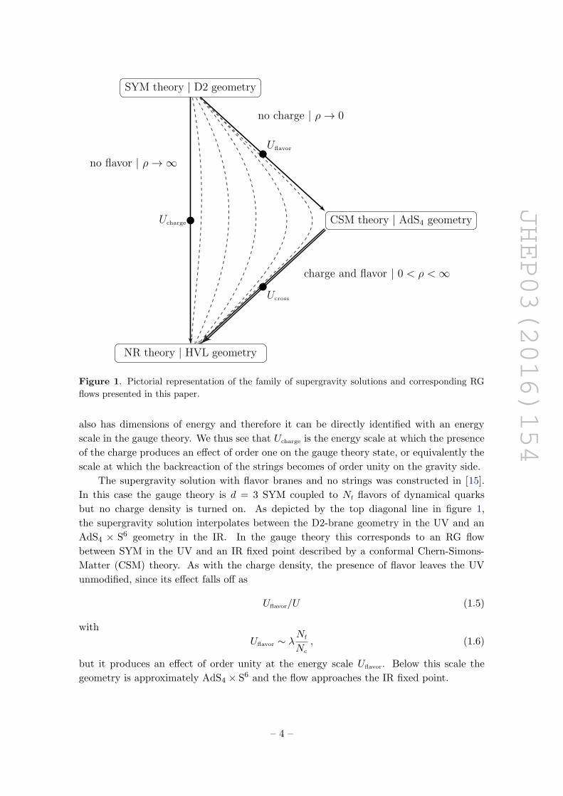
Figure 1. Pictorial representation of the family of supergravity solutions and corresponding RG
flows presented in this paper.
also has dimensions of energy and therefore it can be directly identified with an energy
scale in the gauge theory. We thus see that Ucharge is the energy scale at which the presence
of the charge produces an effect of order one on the gauge theory state, or equivalently the
scale at which the backreaction of the strings becomes of order unity on the gravity side.
The supergravity solution with flavor branes and no strings was constructed in [15].
In this case the gauge theory is d = 3 SYM coupled to Nf flavors of dynamical quarks
but no charge density is turned on. As depicted by the top diagonal line in figure 1,
the supergravity solution interpolates between the D2-brane geometry in the UV and an
AdS4 × S6 geometry in the IR. In the gauge theory this corresponds to an RG flow
between SYM in the UV and an IR fixed point described by a conformal Chern-Simons-
Matter (CSM) theory. As with the charge density, the presence of flavor leaves the UV
unmodified, since its effect falls off as
Uflavor/U (1.5)
with
Uflavor ∼ λNf
Nc
, (1.6)
but it produces an effect of order unity at the energy scale Uflavor. Below this scale the
geometry is approximately AdS4 × S6 and the flow approaches the IR fixed point.
– 4 –
JHEP03(2016)154
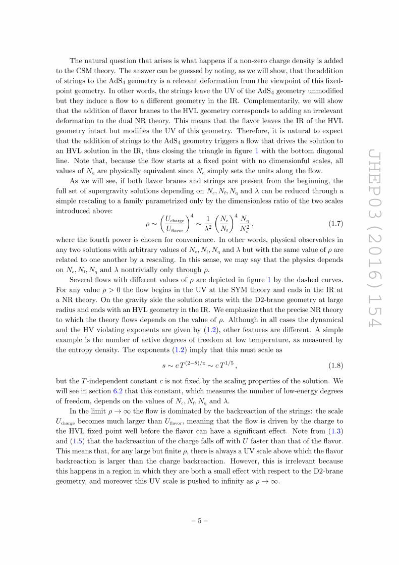
The natural question that arises is what happens if a non-zero charge density is added
to the CSM theory. The answer can be guessed by noting, as we will show, that the addition
of strings to the AdS4 geometry is a relevant deformation from the viewpoint of this fixed-
point geometry. In other words, the strings leave the UV of the AdS4 geometry unmodified
but they induce a flow to a different geometry in the IR. Complementarily, we will show
that the addition of flavor branes to the HVL geometry corresponds to adding an irrelevant
deformation to the dual NR theory. This means that the flavor leaves the IR of the HVL
geometry intact but modifies the UV of this geometry. Therefore, it is natural to expect
that the addition of strings to the AdS4 geometry triggers a flow that drives the solution to
an HVL solution in the IR, thus closing the triangle in figure 1 with the bottom diagonal
line. Note that, because the flow starts at a fixed point with no dimensionful scales, all
values of Nq are physically equivalent since Nq simply sets the units along the flow.
As we will see, if both flavor branes and strings are present from the beginning, the
full set of supergravity solutions depending on Nc, Nf, Nq and λ can be reduced through a
simple rescaling to a family parametrized only by the dimensionless ratio of the two scales
introduced above:
ρ ∼(Ucharge
Uflavor
)4
∼ 1
λ2
(Nc
Nf
)4 Nq
N2c
, (1.7)
where the fourth power is chosen for convenience. In other words, physical observables in
any two solutions with arbitrary values of Nc, Nf, Nq and λ but with the same value of ρ are
related to one another by a rescaling. In this sense, we may say that the physics depends
on Nc, Nf, Nq and λ nontrivially only through ρ.
Several flows with different values of ρ are depicted in figure 1 by the dashed curves.
For any value ρ > 0 the flow begins in the UV at the SYM theory and ends in the IR at
a NR theory. On the gravity side the solution starts with the D2-brane geometry at large
radius and ends with an HVL geometry in the IR. We emphasize that the precise NR theory
to which the theory flows depends on the value of ρ. Although in all cases the dynamical
and the HV violating exponents are given by (1.2), other features are different. A simple
example is the number of active degrees of freedom at low temperature, as measured by
the entropy density. The exponents (1.2) imply that this must scale as
s ∼ c T (2−θ)/z ∼ c T 1/5 , (1.8)
but the T -independent constant c is not fixed by the scaling properties of the solution. We
will see in section 6.2 that this constant, which measures the number of low-energy degrees
of freedom, depends on the values of Nc, Nf, Nq and λ.
In the limit ρ→∞ the flow is dominated by the backreaction of the strings: the scale
Ucharge becomes much larger than Uflavor, meaning that the flow is driven by the charge to
the HVL fixed point well before the flavor can have a significant effect. Note from (1.3)
and (1.5) that the backreaction of the charge falls off with U faster than that of the flavor.
This means that, for any large but finite ρ, there is always a UV scale above which the flavor
backreaction is larger than the charge backreaction. However, this is irrelevant because
this happens in a region in which they are both a small effect with respect to the D2-brane
geometry, and moreover this UV scale is pushed to infinity as ρ→∞.
– 5 –

JHEP03(2016)154
In the opposite limit, ρ → 0, the hierarchy of scales is inverted and the flavor drives
the flow to the AdS4 fixed point before the charge can have a significant effect. If ρ is
very small but non-zero, then the flow is first driven very close to the AdS4 fixed point but
it eventually ‘realizes’ that the charge density is non-zero and is then driven to the HVL
geometry in the deep IR. The scale Ucross at which the transition between AdS4 and HVL
takes place can be determined from the position in the holographic direction where the
backreaction of the strings on the AdS4 geometry becomes of order one. The result is
Ucross ∼ λ3/7
(Nc
Nf
)1/7 (Nq
N2c
)2/7
. (1.9)
Note that this scale is parametrically smaller than Uflavor if ρ 1, since
U4flavor ∼ ρ−1 U4
charge ∼ ρ−8/7 U4cross . (1.10)
Thus in the small-ρ limit the theory exhibits quasi-conformal or ‘walking’ dynamics in the
energy range Ucross U Uflavor.2 In section 5 we will verify this explicitly by showing
that the energy between a pair of external quarks separated a distance L from one another
exhibits the conformal scaling Eqq ∼ 1/L in the energy range above.
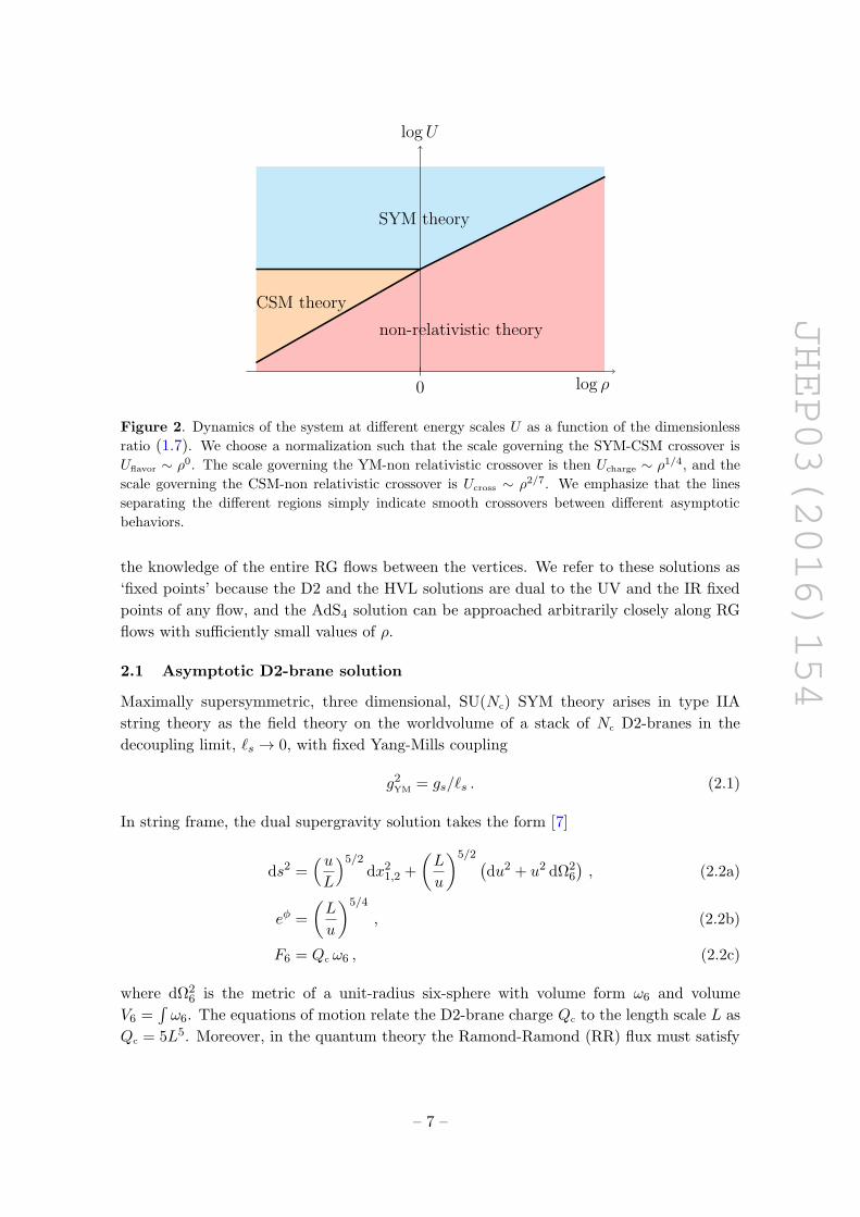
The dynamics of the theory at different energy scales for different values of ρ is sum-
marized in figure 2.
The family of solutions that we will construct provide a set of possible IR behaviors
of the gauge theory under consideration. As we will see, these solutions are thermody-
namically stable and have vanishing entropy density at zero temperature. However, the
possibility that other IR geometries or finite-density phases exist that could compete with
the current ones cannot be discarded. It would be interesting to investigate this possibility
in future work.
This paper is organized as follows. In section 2 we describe the three geometries
corresponding to the vertices of the triangle in figure 1. In section 3 we determine the
crossover scales between these geometries. In section 4 we provide the full numerical
solutions describing the RG flows depicted in figure 1. In section 5 we compute the energy
of a quark-antiquark pair as a function of their separation and prove that, for RG flows with
small ρ, it exhibits the expected quasi-conformal behavior at intermediate separations. In
section 6 we compute the chemical potential, the equation of state and the speed of sound
at zero temperature, as well as the entropy density at low temperature. Finally, in section 7
we explain how the set of RG flows summarized in figure 1 is modified upon the introduction
of a non-zero quark mass.
2 Fixed points
We will now study the solutions corresponding to each of the three vertices in the triangle
of figure 1 and derive the crossover scales between them. This analysis does not require
2In the context of AdS/CMT, examples of d = 3 solutions with walking behavior near an intermediate
fixed point include [21–23].
– 6 –
JHEP03(2016)154
log ρ
logU
0
CSM theory
SYM theory
non-relativistic theory
Figure 2. Dynamics of the system at different energy scales U as a function of the dimensionless
ratio (1.7). We choose a normalization such that the scale governing the SYM-CSM crossover is
Uflavor ∼ ρ0. The scale governing the YM-non relativistic crossover is then Ucharge ∼ ρ1/4, and the
scale governing the CSM-non relativistic crossover is Ucross ∼ ρ2/7. We emphasize that the lines
separating the different regions simply indicate smooth crossovers between different asymptotic
behaviors.
the knowledge of the entire RG flows between the vertices. We refer to these solutions as
‘fixed points’ because the D2 and the HVL solutions are dual to the UV and the IR fixed
points of any flow, and the AdS4 solution can be approached arbitrarily closely along RG
flows with sufficiently small values of ρ.
2.1 Asymptotic D2-brane solution
Maximally supersymmetric, three dimensional, SU(Nc) SYM theory arises in type IIA
string theory as the field theory on the worldvolume of a stack of Nc D2-branes in the
decoupling limit, `s → 0, with fixed Yang-Mills coupling
g2YM = gs/`s . (2.1)
In string frame, the dual supergravity solution takes the form [7]
ds2 =(uL
)5/2dx2
1,2 +
(L
u
)5/2 (du2 + u2 dΩ2
6
), (2.2a)
eφ =
(L
u
)5/4
, (2.2b)
F6 = Qc ω6 , (2.2c)
where dΩ26 is the metric of a unit-radius six-sphere with volume form ω6 and volume
V6 =∫ω6. The equations of motion relate the D2-brane charge Qc to the length scale L as
Qc = 5L5. Moreover, in the quantum theory the Ramond-Ramond (RR) flux must satisfy
– 7 –
JHEP03(2016)154
the quantization condition1
(2π`s)5 gs
∫F6 = Nc , (2.3)
which relates the dimensionful constants Qc and L to the number of colors of the gauge
theory
Qc = 5L5 =(2π`s)
5
V6gsNc . (2.4)
Note that, without loss of generality, the dilaton in (2.2) is normalized in a gs-independent
way, so that the local string coupling is actually gseφ. Consistently, we have included an
explicit factor of gs in (2.3).
The holographic coordinate u in (2.2) has dimensions of length. As explained in [7], it
is useful to define a new radial coordinate
U = u/2π`2s (2.5)
with dimensions of energy which can be directly identified with an energy scale in the
gauge theory. The solution (2.2) provides a valid description in the range in which both
the curvature in string units and the dilaton are small. This region is given by
Udual U Upert , (2.6)
with
Udual ≡ λN−4/5c , Upert ≡ λ , (2.7)
and is parametrically large in the large-Nc limit.
2.2 Hyperscaling-violating Lifshitz solution
Adding a quark density to the SYM theory above is dual on the gravity side to adding a
density of strings appropriately distributed. In the UV this induces a subleading correction
to the solution (2.2) that falls off as in (1.3). In the IR, this drives the theory to an HVL
geometry [17]. Here we summarize the necessary results for the discussion of the crossover
scales; additional details will be presented below.
The metric and dilaton are given by
ds2 =38416
6655 (Qst L)2
[−Ct
r11
L11dt2 +
r3
L3dx2
2 +363
343
L
rQst L
(dr2 +
5
12r2dΩ2
6
)], (2.8a)
eφ =25 73
113
√7/5
(Qst L)5/2
r5/2
L5/2, (2.8b)
where L is the same as in (2.2), Ct is a positive number (determined dynamically by the
RG flow from the UV) that we will discuss further in section 6.2, and the constant
Qst = 2π`2s λNq
N2c
(2.9)
measures the string charge density. The precise numerical factors and the powers of Qst
in (2.8) are such that the reduced four-dimensional metric is of the form given in eq. (1.1)
– 8 –

JHEP03(2016)154
with IR time tIR =√Ct t, and coincides exactly with the solution given in ref. [17]. In
order to compare with the notation in that paper, the reader should note that
Qst
∣∣here
=Q
L
∣∣∣there
. (2.10)
The dynamical and HV exponents of the solution are given by (1.2) and can be read
off from the fact that, in Einstein frame, the metric behaves as
ds2 ∼ r−2θ/D[− r2zdt2 + r2dx2
2 + r−2(dr2 + r2dΩ2
6
) ], (2.11)
with D = 8 the number of spatial directions excluding the holographic direction.3
The metric and the dilaton (2.8) are supported by the RR fluxes
F6 = Qc ω6 = 5L5 ω6 , F2 = Qst dx1 ∧ dx2 , (2.12)
associated to the presence of a stack of D2-branes and a density of strings, respectively. In
order to ensure that the string density of the perturbed D2-brane solution in the UV and
the HVL solution in the IR are the same, as it should be for them to be part of the same RG
flow, we must require that the x-directions are normalized in the same way. This can be
accomplished by matching the IR and the UV forms of the gxx components of the effective,
S6-reduced metric. This leads to the following identification between the IR coordinate
used in (2.8) and the UV coordinate used in (2.2) [17]:
r
L=(uL
)7/2. (2.13)
The range of validity of the solution (2.8), namely the region where both the dilaton
and the curvature in string units are small, is given by
Ulower U Uupper (2.14)
with
Ulower = λ3/7
(Nq
N2c
)2/7
, Uupper = N4/35c Ulower , (2.15)
which is parametrically large in the large-Nc limit.
In order for the region where the geometry transitions between the D2-brane solution
and the HVL solution to be described by type IIA supergravity, we must require that
both (2.6) and (2.14) be satisfied at U = Ucharge, which translates into the following bounds
on the charge density:
λ2N−16/5c Nq
N2c
λ2 . (2.16)
Note that both bounds are compatible with Nq being of order N2c . If the lower bound is
relaxed, then there is a region along the flow where the dilaton is large and the correct
description of that region is provided by eleven-dimensional supergravity.
3Reducing upon the S6 and using D = 2 yields a metric like (1.1) with the same exponents [24].
– 9 –
JHEP03(2016)154
2.3 AdS4 solution
Adding Nf flavors of dynamical quarks to the three-dimensional SYM theory is dual on the
gravity side to adding Nf D6-branes. Ref. [15] constructed the corresponding solution when
the D6-branes are smeared over the S6 directions transverse to the D2-branes in a way that
restores the maximum amount of symmetry compatible with N = 1 supersymmetry. In
the UV this induces a subleading correction to the solution (2.2) that falls off as in (1.5).
In the IR, this drives the theory to a fixed point described by an AdS4 × S6 geometry.
Here we summarize the necessary results for the discussion of the crossover scales; further
details will be given below.
The construction of [15] makes use of the fact that the S6 admits a nearly Kahler
(NK) structure, which implies that it is equipped with a real two-form, J , and a complex
three-form, Ω, satisfying:
dJ = 3 Im Ω , d Re Ω = 2 J ∧ J , (2.17a)
J ∧ Ω = 0 ,1
6J ∧ J ∧ J =
i
8Ω ∧ Ω = ω6 , (2.17b)
∗6J =1
2J ∧ J , ∗6Ω = −iΩ . (2.17c)
A specific construction of J,Ω in a particular coordinate system was given in [15]. These
forms provide a natural basis for writing the RR fluxes of the solution,
F6 = Qc ω6 = 5L5 ω6 , F2 = Qf J , (2.18)
where for massless quarks one has a constant
Qf =2π`2sV2
λNf
Nc
, (2.19)
with V2 =∫J , measuring the number of D6-branes. Alternatively we can view Qf as
characterizing the strength of the backreaction of the flavor branes on the color geometry.
The RR six-form is the same one as in eq. (2.2c), originating from the stack of D2-branes,
whereas the RR two-form violates the Bianchi identity, dF2 6= 0, signalling the presence of
D6-brane sources. The fluxes above support the following metric and dilaton
ds2 =R2
L2IR
dx21,2 +
L2IR
R2
(dR2 +
9
4R2dΩ2
6
), (2.20a)
gs eφ =
(217
54
π2
3
Nc
N5f
)1/4
, (2.20b)
where
LIR = `s
(2
35 π2
Nc
Nf
)1/4
(2.21)
is the AdS4 radius. The requirement that type IIA supergravity provides a reliable de-
scription of this geometry implies that
N1/5c Nf Nc , (2.22)
– 10 –
JHEP03(2016)154
which in turn guarantees that
Udual Uflavor Upert , (2.23)
with Udual, Upert defined as in (2.7). This means that, in fact, the entire flow from the
D2-geometry to the AdS4 geometry is well described by type IIA supergravity.
3 Crossover scales
With the three solutions (2.2), (2.8) and (2.20) in hand, we are now ready to show how the
crossover scales (1.4), (1.6) and (1.9) are determined. As mentioned in section 1, Ucharge and
Uflavor can be determined from the full solutions interpolating between the D2-geometry and
the HVL and AdS geometries, respectively. These solutions are known explicitly enough to
determine the radial positions at which the backreaction of the strings [17] or of the flavor
branes [15] becomes of order unity. Translating between these positions and gauge theory
energy scales leads to (1.4) and (1.6).
Alternatively, one may determine the three crossover scales by equating the dilatons
in the three solutions (2.2), (2.8) and (2.20). This amounts to identifying the crossover
point with the point at which the dilaton changes behavior from one solution to another.
Equating the dilaton in (2.2) and (2.8) and using (2.13) to express both dilatons in terms
of the same radial coordinate u, and then translating this into an energy scale via (2.5),
leads to Ucharge. Equating the dilatons in (2.2) and (2.20) and using again (2.5) leads to
Uflavor. Finally, equating the dilatons in (2.8) and (2.20), using (2.13) to translate from r
to u, and then using (2.5) to translate from u to U , leads to Ucross.
We will now show that the three scales above can also be determined in a third way,
namely by comparing the stress tensor of a D6-brane probe with strings dissolved in it with
the stress tensor supporting the geometry in which the D6-brane is placed. The strategy is
to determine the radial position at which the stress tensor of the brane-plus-strings system
would compete with that of the background geometry. At that point the backreaction
would become of order unity. This will also allow us to show in which geometries the
addition of flavor branes or strings corresponds to a relevant or irrelevant deformation on
the field theory side.
For the purposes of this discussion it suffices to consider the Dirac-Born-Infeld (DBI)
part of the D6-brane action (see the paragraph below eq. (3.11) for the justification). This
takes the form
SDBI = −TD6
∫d7ξ e−φ
√−P [G] + F (3.1)
with
TD6 =1
(2π`s)6 gs`s(3.2)
the tension of the brane, P[· · · ] the pullback of a spacetime object in string frame to the
worldvolume of the brane,
F = P[B] + 2π`2s dA , (3.3)
– 11 –

JHEP03(2016)154
B the Neveu-Schwarz (NS) two-form and A the BI gauge potential. We assume that the
probe brane wraps an equatorial S3 ⊂ S6 and is extended along the Minkowski and radial
directions. The presence of strings dissolved inside the brane is encoded in an electric BI
potential of the form
A = At(y)dt , (3.4)
with y the holographic radial coordinate. For backgrounds of the form
ds2 = Gtt(y) dt2 +Gxx(y) dx22 +Gyy(y) dy2 +GΩΩ(y) dΩ2
6 (3.5)
with a vanishing B-field, which includes (2.2), (2.8) and (2.20), the DBI action reduces to
SDBI = −2π2 TD6
∫d3x dy e−φ
√−(GttGyy + (2π`2s)
2A′2t)G2xxG
3ΩΩ , (3.6)
where we have integrated out the three sphere angles, thus producing the 2π2 factor. Since
At enters only via its derivative, the solution for this field can be written in terms of a
constant of integration, nq, as
2π`2s A′t =
√n2
q|Gtt|Gyyn2
q + (2π2 TD6 2π`2s)2e−2φG2
xxG3ΩΩ
. (3.7)
This constant is precisely the string density on the probe, and will play an important role
in the rest of the paper. Note that we use a lower-case symbol to distinguish the string
density on the probe from that in the background. To work at fixed charge density we
perform a Legendre transform in (3.6), and express the action in terms of nq instead of At,
obtaining
SDBI = −2π2 nf TD6
∫d3x dy e−φ
√−GttG2
xxGyyG3ΩΩ
√1 +
e2φ n2q
(2π2 TD6 nf 2π`2s)2G2
xxG3ΩΩ
,
(3.8)
where we have included factors of nf to account for the possibility of multiple overlapping
probe branes. Finally, we compute the stress tensor associated to the D6-brane action.
Since the only non-zero component of the gauge field is the temporal one, we focus on the
time-time component of the stress tensor. This takes the form
Ttt =−2√−G
G2tt
δSDBI
δGtt= 2π2 TD6 nf e
−φ Gtt
G3/2ΩΩ
√1 +
e2φ n2q
(2π2 TD6 nf 2π`2s)2G2
xxG3ΩΩ
, (3.9)
where the tilde is a reminder that this is the probe’s stress tensor. Our goal is to compare
this result to the supergravity stress tensor supporting each of the solutions (2.2), (2.8)
or (2.20), namely to the right-hand side of Einstein’s equations
1
κ2Eµν = e2φ Tµν , (3.10)
where1
2κ2=
2π
(2π`s)8g2s
, (3.11)
Eµν is the Einstein tensor and the factor of e2φ appears because we are working in
string frame.
– 12 –
JHEP03(2016)154
Eqs. (3.7) and (3.9) would not be modified if we had included the Wess-Zumino (WZ)
part of the D6-brane action in our discussion. The reasons are, first, that for the back-
grounds of interest in this section the WZ term does not contain any At-dependent con-
tributions that could modify our definition (3.7) of nq and, second, that the WZ term is
topological, i.e. metric-independent, and therefore it does not contribute to our definition
of the probe stress tensor (3.9).
We are now ready to determine the crossover scales by comparing the stress tensors.
We begin with the D2-brane geometry (2.2). The probe stress tensor behaves as
e2φ Ttt 'nf TD6
L5u2 at zero nq , (3.12a)
e2φ Ttt '1
L5 `2s
nq
u+O(u5) for small u at non-zero nq , (3.12b)
e2φ Ttt 'nf TD6
L5u2 +O(u−4) for large u at non-zero nq , (3.12c)
whereas the supergravity stress tensor scales as
1
κ2Ett '
1
κ2
u3
L5. (3.13)
Consider first nq = 0. In this case we see that the probe stress tensor is subleading at large
u, meaning that the flavor branes are a small correction in the UV. The scale at which their
stress tensor becomes comparable to the background stress tensor is u = uflavor such that
1
κ2
u3flavor
L5∼ nf TD6
L5u2
flavor . (3.14)
Via (2.5) this leads precisely to (1.6) with Nf replaced by nf. This is as expected, since
this is the scale at which the backreaction of the nf flavor probe branes would become
important if we were to include it.
Consider now nq 6= 0. We see that the presence of the strings does not change the
UV behavior of the probe stress tensor, meaning that the backreaction of the strings is
subleading with respect to that of the flavor branes in this regime. This is consistent with
the fall-offs (1.3) and (1.5) mentioned in section 1, and with the fact that the UV geometry
is unmodified even in the presence of both charge and flavor. In contrast, in the IR we see
that the stress tensor of the brane is dominated by the string density, since the 1/u leading
term is proportional to nq and nf-independent, and that this would actually dominate over
the supergravity stress tensor. This is consistent with the fact that the addition of charge
always changes the IR geometry completely, and it drives the RG flow to an HVL solution.
The scale at which the crossover takes place is u = ucharge such that
1
κ2
u3charge
L5∼ 1
L5 `2s
nq
ucharge
, (3.15)
which via (2.5) leads precisely to (1.4) with Nq replaced by nq, as expected.
– 13 –
JHEP03(2016)154
We now turn to the HVL geometry. The probe stress tensor reads
e2φTtt 'nf TD6 Ct
(Qst L)3 L3
r12
L12at zero nq , (3.16a)
e2φTtt 'nq Ct
`2s (Qst L)2 L6
r10
L10+O(r14) for small r at non-zero nq , (3.16b)
e2φTtt 'nf TD6 Ct
(Qst L)3 L3
r12
L12+O(r8) for large r at non-zero nq , (3.16c)
whereas the supergravity stress tensor is
1
κ2Ett ∼
1
κ2
Ct
(Qst L)L2
r10
L10. (3.17)
We see that at small r the probe stress tensor is dominated by the string contribution,
meaning that the addition of flavor leaves the IR geometry unmodified, in agreement with
our previous discussion. Moreover, this string contribution in the IR scales exactly in
the same way as the supergravity stress tensor. This is consistent with the fact that the
HVL geometry is sourced by strings, with only subleading contributions from the flavor
branes. The radial position rcross at which the contribution of the flavor to the probe
stress tensor becomes comparable to that of the strings, and of course also to that of the
background, determines the crossover scale between the string-dominated HVL geometry
and the flavor-dominated AdS4 solution. This position obeys
1
κ2
Ct
(Qst L)L2
r10cross
L10∼ nf TD6 Ct
(Qst L)3 L3
r12cross
L12. (3.18)
Using (2.13) and (2.5) this leads to (1.9) with Nf replaced by nf, as expected.
Finally, we turn to the AdS4 solution. The probe stress tensor is
e2φ Ttt ∼nf TD6
g2s `
5sNc
R2 at zero nq , (3.19a)
e2φ Ttt 'nq
g2s `
8s Nf Nc
+O(R4) for small R at non-zero nq , (3.19b)
e2φ Ttt 'nf TD6
g2s `
5s Nc
R2 +O(R−2) for large R at non-zero nq , (3.19c)
whereas the supergravity stress tensor reads
1
κ2Ett ∼
1
κ2
R2
L4IR
. (3.20)
If nq = 0 the probe stress tensor scales in the same way as the background stress tensor,
consistently with the fact that in this case the background is sourced by a large collection
of flavor branes. This remains true at large R even if nq 6= 0, meaning that the addition
of charge leaves the UV of the AdS4 geometry unmodified. In contrast, at small R the
strings contribution dominates the probe tensor, and this dominates over the background
stress tensor. This confirms that the addition of strings is a relevant deformation from the
– 14 –
JHEP03(2016)154
viewpoint of the fixed point dual to the AdS4 geometry that drives the theory to a new IR
geometry. The scale at which the crossover between the two geometries takes place can be
determined by comparing (3.19b) to (3.20), with the result
Rcross ∼n1/2
q `2sNf
. (3.21)
Note that, from the AdS4 prespective, the dependence on nq is fixed by dimensional anal-
ysis, since this is the only scale at this fixed point. In other words, the theory at this fixed
point has lost any memory of the other dimensionful parameter in the gauge theory, the ’t
Hooft coupling λ. This means that from the AdS4 viewpoint all values of nq are equivalent:
they simply set the units in which all other scales such as the crossover scale (3.21) are
measured. The dependence on λ is recovered when the AdS4 coordinate R is mapped to
the IR coordinate r and then to the UV coordinate u via (2.13). As usual, the relation be-
tween r and R is established by matching the gxx components of the dimensionally reduced
metrics, which gives
r
L=
(27
8
gs L2IR
L3
N5/4f
N1/4c
R
)2
. (3.22)
This relation together with (2.13) and (2.5) maps Rcross to Ucross.
4 Full solutions
We finally turn to the main result of our paper: the family of supergravity solutions dual
to three-dimensional SU(Nc) SYM in the presence of Nf flavors of dynamical quarks and
a non-zero quark density Nq. The flavor branes and the strings act as sources for both
the RR fields and the H-field, and hence they modify their equations of motion. For the
RR fields, through the Hodge-duality relations that these fields obey, this also leads to
a modification of their Bianchi identities, and therefore to a modification of their very
definition in terms of gauge potentials. The full action in the presence of these sources is
discussed in appendix A, to which we refer the reader for additional details.
4.1 Ansatz
The full action of the system consists of type IIA supergravity coupled to a set of D6-branes
with strings dissolved inside them:
S = SIIA + SD6 . (4.1)
The supergravity action is the sum of the NS and the RR sectors,
SIIA = SNS + SRR . (4.2)
Similarly, the D6-action is the sum of the DBI and the WZ terms:
SD6 = SDBI + SWZ . (4.3)
– 15 –
JHEP03(2016)154
As we will explain below, the presence of the strings will not change the fact that the
metric in the solution is invariant under the full isometry group of the S6, just like when only
flavor but no charge is present [15]. This means that the most general metric compatible
with the symmetries of our system takes the form (3.5), and also that the solution is
naturally equipped with the forms J and Ω obeying the relations (2.17) associated to the
NK structure of the S6.
The brane action describes a collection of Nf D6-branes appropriately smeared over
the S6 internal directions of the geometry, with a density of strings appropriately smeared
within each D6-brane. In the limit in which the number of branes and strings is large, one
can approximate their distribution by a continuous function, which will allow us to turn
the seven-dimensional D6-brane action into an integral over all spacetime directions. The
information about the orientation and the density of branes at each point is encoded in
the so-called smearing three-form Ξ that will be determined below. In order to write the
smeared DBI part of the action, let us first rewrite the DBI action for a single brane (3.1) as
SDBI = −TD6
∫D6P [K] , (4.4)
where the seven-form K is defined as
K = e−φ√− det (G+ F) dt ∧ dx1 ∧ dx2 ∧ dy ∧ Re Ω . (4.5)
In terms of K and the smearing form, the DBI action for the smeared set of branes takes
the form
SDBI = −TD6
∫K ∧ Ξ . (4.6)
Similarly, while the WZ part of the action for a single brane is given by
SWZ = TD6
∫D6LWZ , (4.7)
the smeared action is
SWZ = TD6
∫LWZ ∧ Ξ . (4.8)
The form of LWZ can be found in appendix A.
In order to model the presence of the strings, the BI field on the branes takes the same
form as in (3.4). Note that the fact that the BI electric field only depends on the radial
coordinate y implies that the distribution of the strings respects the full isometry group of
the S6. As we will see below, the NS field B will vanish in our solution, meaning that
F = 2π`2s dA = 2π`2s A′t(y) dy ∧ dt . (4.9)
This implies that F ∧ F = 0, which leads to a simplification with respect to the general
setup discussed in appendix A. Through the WZ part of the branes’ action, F modifies the
equations of motion for the RR field strengths F8 and F6 with respect to pure supergravity
without sources. Equivalently, it modifies the Bianchi identities for their Hodge duals
F2 = − ∗ F8 , F4 = ∗F6 , (4.10)
– 16 –
JHEP03(2016)154
which in the presence of the D6-branes and the strings read
dF2 = −2κ2 TD6 Ξ , (4.11a)
dF4 = H ∧ F2 − 2κ2 TD6F ∧ Ξ . (4.11b)
The first equation is commonly referred to as the ‘violation’ of the Bianchi identity for F2,
and it expresses the simple fact that D6-branes are magnetic sources for F2. This violation
was already present in the case of flavor without strings discussed in [15]. In contrast, the
second term on the right-hand side of the Bianchi identity for F4 was not present for the
solutions with strings but without flavor studied in [17]. Indeed, this term is only present
when the system contains both strings and D6-branes, since it comes from the electric
components of C5 sourced by the term ∫C5 ∧ F (4.12)
contained in the WZ part of the D6-branes’ action. Through the duality relations (4.10)
these electric components give rise to the second term on the right-hand side of dF4. We
thus see that, although it is the string density represented by F that sources C5, the
presence of the D6-branes is necessary since the coupling between F and C5 is supported
on their worldvolume.
We are now ready to specify the ansatz for our solution and to integrate the corre-
sponding equations of motion. We begin with the RR forms. We choose to specify directly
F2 and F6; their Hodge duals F4 and F8 can be obtained via (4.10). Our ansatz for F2 is
F2 = Qst dx1 ∧ dx2 +Qf J . (4.13)
This is the most general form compatible with the symmetries of our system, in particular
with the SU(3) structure of the S6, except for the fact that we have omitted a term
proportional to dt ∧ dy. This term is allowed by symmetry considerations, but we will
show below that it must vanish by virtue of the equation of motion for the B-field. As we
will see, the constant Qst is related to the string density [25]. Similarly, Qf is related to
the distribution of D6-branes along the radial direction. If some of the quark flavors in the
gauge theory are massive, then Qf becomes a function of the radial direction, Qf(y). Here we
will restrict ourselves to the case in which all quarks are massless, which translates into the
fact that Qf is a constant related to the number of D6-branes through (2.19). Computing
dF2 with (4.13) and (2.17) and comparing to (4.11a) we deduce that the smearing form is
Ξ = − 3Qf
2κ2 TD6
Im Ω . (4.14)
In order to specify F6, we first note from (4.9) and (4.14) that the coupling in (4.12)
implies that C5 must contain a term of the following form:
C5 ⊃ B(y) dx1 ∧ dx2 ∧ Re Ω . (4.15)
– 17 –
JHEP03(2016)154
Including also the term necessary to account for the presence of D2-branes in the solution,
as in (2.2c), we see that F6 must take the form
F6 =Qc
6J ∧ J ∧ J + B′ dy ∧ dx1 ∧ dx2 ∧ Re Ω + 2B dx1 ∧ dx2 ∧ J ∧ J , (4.16)
where ′ denotes differentiation with respect to y and we have used (2.17) to write the
volume form on the six-sphere in terms of J . The constant Qc is related to the number
of D2-branes through (2.4). The equation of motion for the function B(y) is obtained by
Hodge-dualizing F6 to F4 with the metric (3.5), which yields
F4 = Qc
√−GttGyy Gxx
G3ΩΩ
dt ∧ dx1 ∧ dx2 ∧ dy
+ 4B√−GttGyyGxxGΩΩ
dt ∧ dy ∧ J
+ B′√−Gtt√Gyy Gxx
dt ∧ ImΩ , (4.17)
and then substituting into the Bianchi identity (4.11b). The result is
∂y
(√−GttGyy
B′
Gxx
)− 12
√−GttGyyGxxGΩΩ
B − 3Qf 2π`2s A′t = 0 . (4.18)
The physical meaning of the ‘magnetic potential’ B is more easily understood by rewriting
it in terms of an electric, dual potential. For this purpose, we write the following ansatz
for the three-form RR potential:
C3 = C3 + C(y) dt ∧ J , (4.19)
where C3 is the usual piece associated to the presence of D2-branes that obeys
dC3 = Qc
√−GttGyy Gxx
G3ΩΩ
dt ∧ dx1 ∧ dx2 ∧ dy . (4.20)
Substituting dC3 in the definition (A.19) of the modified field strength F4 and comparing
to (4.17) we see that C(y) and its first derivative must satisfy the equations
C = −1
3
√−GttGyy
B′
Gxx, C′ +Qf 2π`2s A
′t = −4
√−GttGyyGxxGΩΩ
B . (4.21)
These equations allow us to eliminate B in favor of C and vice versa. The term in C3
proportional to C can now be interpreted as associated to D2-branes wrapped on the cycle
threaded by J . Upon reduction along the compact directions, this gives rise to a massive
vector field with positive mass squared.4 Therefore the field C(y) is dual to (the time
component of) an irrelevant vector operator constructed out of adjoint fields in the gauge
4An analogous field was present in the four-dimensional case of [26] and its dual interpretation around
the AdS5 region was given in [27].
– 18 –
JHEP03(2016)154
theory. This should be contrasted with the vector field A on the D6-branes, which is dual
to a conserved, and therefore marginal, current operator in the gauge theory constructed
out of the microscopic fields in the fundamental representation of the gauge group. Below
we will have more to say about the interplay between these two vector fields.
We now turn to the equation of motion for the B-field. This may be written as
d(e−2φ ∗H
)=δS
δB, (4.22)
where the right-hand side includes all variations with respect to B but not dB, and is
given by
δS
δB= F2 ∧ ∗F4 +
1
2F4 ∧ F4 (4.23)
+ 2κ2 T6 e−φ√G2xxG
3ΩΩ
2π`2s A′t√
− (GttGyy + (2π`2sA′t)
2)dx1 ∧ dx2 ∧ Re Ω ∧ Ξ .
The second line in this equation is the DBI contribution. We will solve this equation with
B = H = 0, which immediately implies that the term proportional to dt ∧ dy allowed by
symmetry considerations in (4.13) must vanish. At first sight it may seem surprising that
the presence of strings does not automatically lead to a non-zero H, but the non-linearities
of supergravity imply that the H sourced by the strings can be exactly cancelled by the
H sourced by the products of RR forms in (4.23). Requiring this cancellation fixes the BI
field on the D6-branes to
2π`2s A′t =
√−GttGyy
eφG−3/2ΩΩ (Qc Qst + 12Qf B)√
(12Qf Gxx)2 + e2φG−3ΩΩ (Qc Qst + 12Qf B)2
. (4.24)
To close the circle we note that (4.24) is automatically a solution of the equation of
motion for the BI field obtained by varying the full action with respect to A. The reason is
that dA always appears together with B in the gauge-invariant combination dA+B. This
means thatδS
δdA=δS
δB(4.25)
and therefore that the equation of motion for A,
dδS
δdA= 0 , (4.26)
is automatically implied by the exterior derivative of (4.22). In fact, substituting (4.24)
in (4.23) gives the explicit result for the so-called electric displacement
δS
δdA= 2π`2s
Qc Qst
2κ2dx1 ∧ dx2 ∧ ω6 . (4.27)
The string density in the x1 − x2 directions is obtained by integrating this expression over
the six-sphere,
Nq dx1 ∧ dx2 =
∫S6
δS
δdA, (4.28)
– 19 –
JHEP03(2016)154
which finally yields the relation between the string density and Qst:
Qst =2κ2
Qc
Nq
2π`2s V6= 2π`2s λ
Nq
N2c
. (4.29)
Note that Nq is the total string density in the system, whereas the string density per
D6-brane is qst = Nq/Nf. Thus one may formally consider a limit in which the number of
D6-branes goes to zero and the string density per D6-brane diverges in such a way that
the total string density is kept fixed:
Nf → 0 , qst →∞ , Nq fixed . (4.30)
In this limit B = 0 and the model presented in this section reduces to the one in [17],
which describes the flow along the vertical line on the left-hand side of the triangle in
figure 1. In particular, the DBI term (4.6) reduces to a smeared Nambu-Goto action for a
uniform distribution of strings stretching along the radial direction. In the opposite limit
in which we set Qst = B = 0 the model of this section reduces to that of [15], where the
supersymmetric flow with flavor but no charge represented by the upper diagonal edge of
the triangle in figure 1 was constructed.
4.2 Scalings
In principle, the physics in our system depends on the four parameters λ,Nc, Nf and Nq.
However, through appropriate rescalings we will now see that the physics depends non-
trivially only on a dimensionless combination of these parameters. In order to show this,
it is useful to begin by recalling the length dimensions of the dimensionful variables in
our set-up:
[y] ∼ ` , [Qc] ∼ `5 , [Qf] ∼ ` , [Qst] ∼ `−1 , [B] ∼ `3 , [GΩΩ] ∼ `2 , [At] ∼ `−1 .
(4.31)
The metric components Gtt, Gxx, Gyy and the dilaton are dimensionless.
In order to work with dimensionless quantities we need to choose a specific unit of
length. Any combination of Qc, Qf and Qst with length dimensions is a valid choice, and
we find it convenient to simply use Qf (which implies that taking the Nf → 0 limit in the
dimensionless variables is not straightforward). We thus write the radial coordinate and the
dimensionful functions in our ansatz in terms of the following dimensionless counterparts:
y = Qf y , GΩΩ = Q2f GΩΩ , B = Q3
f B . (4.32)
The reason for using a tilde on GΩΩ instead of an overline will become clear shortly.
Upon implementing this transformation in the radicand in eq. (4.24), we observe that the
following dimensionless quantity measures the effect of the charge density:
ρ ≡ Qc Qst
12Q4f
=π2 V 4
2
3V6
1
λ2
(Nc
Nf
)4 Nq
N2c
, (4.33)
where we recall that V2 and V6 are dimensionless volumes. Note that all the dependence
on the string theory parameters `s, gs has cancelled, indicating that ρ is directly a gauge
theory parameter. We will now show that the physics depends non-trivially only on this
parameter.
– 20 –
JHEP03(2016)154
In order to do so, we rescale some of our functions with the following powers of the
second dimensionless quantity Qc/Q5f :
Gtt =
(Qc
Q5f
)−1/2
Gtt , Gxx =
(Qc
Q5f
)−1/2
Gxx , (4.34a)
Gyy =
(Qc
Q5f
)1/2
Gyy , GΩΩ =
(Qc
Q5f
)1/2
GΩΩ , (4.34b)
eφ =
(Qc
Q5f
)1/4
eφ . (4.34c)
Note that GΩΩ gets rescaled to its final counterpart GΩΩ. Through eq. (4.24), the rescalings
above imply that A′t does not get rescaled i.e. that
A′t = A′t (4.35)
with
2π`2s A′t =
√−GttGyy
eφG−3/2ΩΩ
(ρ+ B
)√G
2xx + e2φG
−3ΩΩ
(ρ+ B
)2 . (4.36)
When the original functions and radial coordinate are replaced by their overlined coun-
terparts, all the dependence on Qf and Qc in the action (4.1) cancels out, leaving behind
only a dependence on ρ except for an overall factor of Q5f in front of the action. The ef-
fective gravitational coupling Q5f /2κ
2 thus has dimension `−3, since the only dimensionful
coordinates to integrate over after the rescaling are the three Minkowski coordinates. This
result means that the equations of motion in terms of the rescaled variables depend only
on ρ, as we wanted to show. In fact, by performing a further rescaling of the form
Gxx → ρGxx , B → ρB , (4.37)
we could eliminate the dependence on ρ from the equations of motion, but only at the
expense of introducing ρ dependence in the boundary conditions. We will therefore not
perform this rescaling.
We conclude that only the parameter ρ distinguishes inequivalent RG flows (i.e. flows
that cannot be mapped to one another by simple rescalings) in the space of theories
parametrized by λ,Nc, Nf and Nq. This parameter can be naturally understood as the
ratio between the typical energy scales associated to charge and flavor, as anticipated in
eq. (1.7). Unless stated otherwise, in the rest of the paper we will work with the dimen-
sionless (overlined) variables, and we will omit the overlines for simplicity. The full set of
equations of motion written in terms of these variables can be found in appendix B.
4.3 Numerical integration
In this section we will provide an overview of how we integrated the equations of motion
numerically, relegating some technical details and long equations to appendix C. We will
begin with equations in which λ,Nc, Nf and Nq have not been eliminated yet, and later
we will explain how to exploit the fact that the physics only depends on ρ to construct
the solutions.
– 21 –
JHEP03(2016)154
To obtain a numerical solution, it is convenient to parametrize the string-frame metric
and the dilaton as
ds2 = h−12(−f1dt2 + dx2
2
)+ h
12 e2χ
(dy2
f2+ y2ds2
6
),
eφ = h14 e3χg , (4.38)
where f1, f2, h, χ and g depend only on the radial coordinate y. This choice of parametriza-
tion is motivated by the fact that it generalizes that of the chargeless case [15] by allowing
for the breaking of Lorentz invariance expected in the presence of a charge density. Using
diffeomorphism invariance, we fix the radial coordinate by setting
h =Qc
5y5, (4.39)
as in the D2-brane solution. Fixing the form of h allows us to solve algebraically for the
function f2, whose expression is given in (C.1). Moreover, the gauge field At on the D6-
branes can be solved for in terms of the other functions, as given in (C.3), and eliminated
from the remaining equations.
We are thus left with a set (C.4) of four coupled, second-order differential equations
for f1, χ, g and B that we must solve numerically, subject to the boundary conditions that
they interpolate between the D2-brane solution in the UV and the HVL solution in the IR.
The asymptotic solution in the UV, eq. (C.5), depends on four undetermined constants
associated to the VEVs of the following four operators: the stress tensor, TrF 2, TrF 4, and
the operator dual to B. Similarly, the asymptotic solution in the IR (C.6) depends on
another four undetermined constants. The match between the number of undetermined
constants is a necessary consistency check for the existence of solutions connecting these
two asymptotic behaviors.
A further consistency check comes from requiring the existence of flows that come very
close to the AdS4 fixed point in figure 1. Any such flow must be driven from the fixed
point to the UV by modes that grow (or at least stay constant) towards the UV, and from
the fixed point to the IR by modes that grow (or at least stay constant) towards the IR.
This immediately implies that the fields that are turned on around the fixed point cannot
be dual to relevant operators. Indeed, a field dual to an operator of dimension ∆ behaves
as a combination of %d−∆ (dual to a source) and %−∆ (dual to a VEV), where % is the
usual Fefferman-Graham coordinate and the AdS boundary is at % → ∞. For a relevant
operator both modes decay towards the UV and grow towards the IR, so the presence
of such an operator would preclude the necessary matching. In contrast, irrelevant or
marginal operators are allowed. In appendix D we compute the spectrum of fluctuations
around the AdS4 fixed point and verify that no relevant operator is turned on.
We choose to solve the system of four coupled second-order ODEs using a relaxation
method. We begin by compactifying the radial coordinate using the transformation
y =1 + Y
1− Y, (4.40)
– 22 –
JHEP03(2016)154
so that our functions are defined on the domain Y ∈ [−1, 1]. For numerical convenience,
we redefine the unknown functions by removing their IR scaling behavior as follows:
B =
(1 + Y
2
)10/3
B , (4.41a)
f1 =
(1 + Y
2
)20/3
f1 , (4.41b)
g =
(1 + Y
2
)4/3
g , (4.41c)
eχ =
(1 + Y
2
)2/3
eχ . (4.41d)
The advantage of this redefinition lies in the fact that it simplifies the implementation of
the boundary conditions. To be more precise, the boundary conditions that we need to
impose are
B, f1, g, eχ = 0, 1, 1, 1 (4.42)
in the UV (Y = 1) andB, f ′1, g, eχ = − 3 · 52/3Qf
(14QcQst)1/3, 0,
51/6142/3
√11(QcQst)1/3
,101/3
(7QcQst)1/6
(4.43)
in the IR (Y = −1). Note that we are fixing the derivative of f1 to zero in the IR. The
value of f1 itself in the IR is determined by the flow and is given by the constant Ct
in eq. (C.6). We will see below that this constant plays an important role in the low-
temperature thermodynamics of the system.
We proceed by evenly discretising the coordinate Y to form a lattice and we approx-
imate the derivatives of our functions at each lattice point using a fourth-order finite-
difference scheme.5 The problem is then reduced to solving a set of non-linear algebraic
equations for the values of each function at each point on the grid. This is done using the
Newton-Raphson method: one starts with an initial guess for the unknown functions at
each lattice point, which presumably does not solve the differential equations, and then
iteratively improves the guess in order to obtain functions that solve the equations to the
desired accuracy.
Given the scaling (4.34), we can restrict our attention without loss of generality to
solutions with Qc = Qst = 1 and 0 < Qf < ∞. Each of these solutions then provides
a representative of a flow with a value of ρ given by ρ = 1/12Q4f , from which the most
general solution with arbitrary values of all the parameters can be obtained through the
rescalings discussed in section 4.2. The strategy for finding these solutions is to start by
picking Qf = 0 (B = 0), describing the flow [17] between the D2-brane in the UV and the
HVL in the IR, and then slightly deform this solution by introducing a small amount of
flavor. This is feasible because in both cases the end points of the integration are the same.
5We choose to work with finite differences over pseudospectral methods because of the logarithms that
appear in the UV expansion (C.5).
– 23 –
JHEP03(2016)154
Once a solution with a small but non-vanishing Qf is obtained, one can slowly increase the
flavor using the previous solution as an initial guess for the next one. The profiles of the
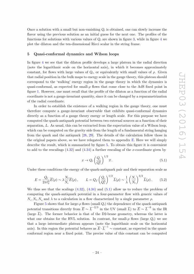
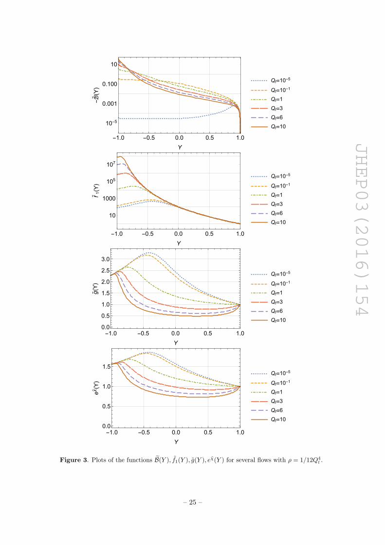
functions for solutions with various values of Qf are shown in figure 3, while in figure 4 we
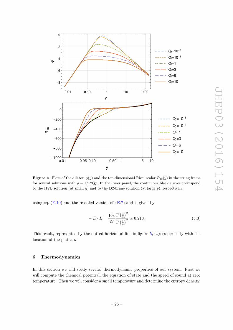
plot the dilaton and the ten-dimensional Ricci scalar in the string frame.
5 Quasi-conformal dynamics and Wilson loops
In figure 4 we see that the dilaton profile develops a large plateau in the radial direction
(note the logarithmic scale on the horizontal axis), in which it becomes approximately
constant, for flows with large values of Qf, or equivalently with small values of ρ. Given
that radial position in the bulk maps to energy scale in the gauge theory, this plateau should
correspond to the ‘walking’ energy region in the gauge theory in which the dynamics is
quasi-conformal, as expected for small-ρ flows that come close to the AdS fixed point in
figure 1. However, one must recall that the profile of the dilaton as a function of the radial
coordinate is not a gauge-invariant quantity, since it can be changed by a reparametrization
of the radial coordinate.
In order to establish the existence of a walking region in the gauge theory, one must
therefore compute a gauge-invariant observable that exhibits quasi-conformal dynamics
directly as a function of a gauge theory energy or length scale. For this purpose we have
computed the quark-antiquark potential between two external sources as a function of their
separation, L. As usual, this can be extracted from the expectation value of a Wilson loop,
which can be computed on the gravity side from the length of a fundamental string hanging
from the quark and the antiquark [28, 29]. The details of the calculation follow those in
the original papers above, so we have relegated them to appendix E. Here we will simply
describe the result, which is summarized by figure 5. To obtain this figure it is convenient
to add to the rescalings (4.32) and (4.34) a further rescaling of the x-coordinate given by
x→ Qf
(Qc
Q5f
)1/2
x . (5.1)
Under these conditions the energy of the quark-antiquark pair and their separation scale as
E =Qf
2π`2sE(ρ) ∼ λNf
Nc
E(ρ) , L = Qf
(Qc
Q5f
)1/2
L(ρ) ∼ 1
λ
(Nc
Nf
)3/2
L(ρ) . (5.2)
We thus see that the scalings (4.32), (4.34) and (5.1) allow us to reduce the problem of
computing the quark-antiquark potential in a four-parameter flow with generic values of
Nc, Nf, Nq and λ to a calculation in a flow characterized by a single parameter ρ.
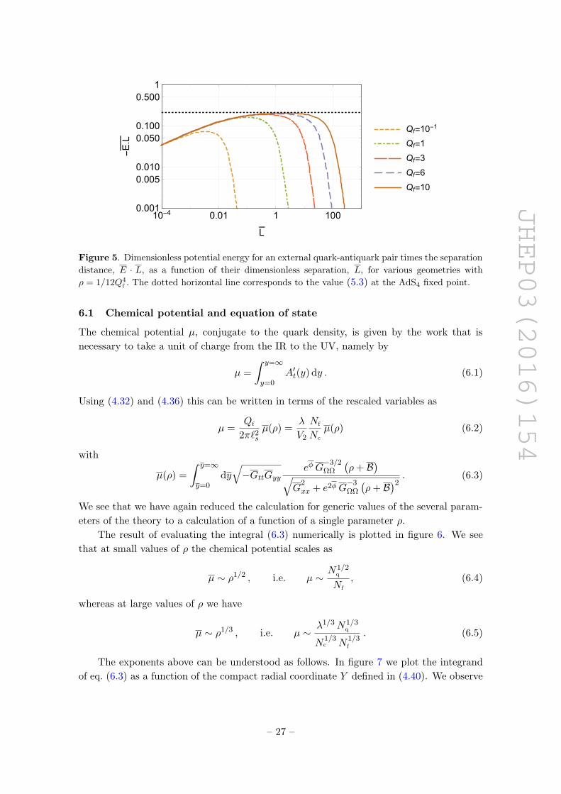
Figure 5 shows that for large-ρ flows (small Qf) the dependence of the quark-antiquark
potential transitions directly from E ∼ L−2/3
in the UV (small L) to E ∼ L−6
in the IR
(large L). The former behavior is that of the D2-brane geometry, whereas the latter is
what one obtains for the HVL solution. In contrast, for small-ρ flows (large Qf) we see
that a large intermediate plateau appears (note the logarithmic scale on the horizontal
axis). In this region the potential behaves as E ·L−1 ∼ constant, as expected in the quasi-
conformal region near a fixed point. The precise value of this constant can be computed
– 24 –
JHEP03(2016)154
-1.0 -0.5 0.0 0.5 1.0
10-5
0.001
0.100
10
Y
-ℬ˜(Y)
Qf=10-5
Qf=10-1
Qf=1
Qf=3
Qf=6
Qf=10
-1.0 -0.5 0.0 0.5 1.0
10
1000
105
107
Y
f˜1(Y)
Qf=10-5
Qf=10-1
Qf=1
Qf=3
Qf=6
Qf=10
-1.0 -0.5 0.0 0.5 1.00.0
0.5
1.0
1.5
2.0
2.5
3.0
Y
g˜(Y)
Qf=10-5
Qf=10-1
Qf=1
Qf=3
Qf=6
Qf=10
-1.0 -0.5 0.0 0.5 1.00.0
0.5
1.0
1.5
Y
eχ∼
(Y)
Qf=10-5
Qf=10-1
Qf=1
Qf=3
Qf=6
Qf=10
Figure 3. Plots of the functions B(Y ), f1(Y ), g(Y ), eχ(Y ) for several flows with ρ = 1/12Q4f .
– 25 –
JHEP03(2016)154
0.01 0.10 1 10 100
-8
-6
-4
-2
0
y
ϕQf=10-5
Qf=10-1
Qf=1
Qf=3
Qf=6
Qf=10
0.01 0.05 0.10 0.50 1 5 10-1000
-800
-600
-400
-200
0
y
R10
Qf=10-5
Qf=10-1
Qf=1
Qf=3
Qf=6
Qf=10
Figure 4. Plots of the dilaton φ(y) and the ten-dimensional Ricci scalar R10(y) in the string frame
for several solutions with ρ = 1/12Q4f . In the lower panel, the continuous black curves correspond
to the HVL solution (at small y) and to the D2-brane solution (at large y), respectively.
using eq. (E.10) and the rescaled version of (E.7) and is given by
− E · L =16π
27
Γ(
34
)2Γ(
14
)2 ' 0.213 . (5.3)
This result, represented by the dotted horizontal line in figure 5, agrees perfectly with the
location of the plateau.
6 Thermodynamics
In this section we will study several thermodynamic properties of our system. First we
will compute the chemical potential, the equation of state and the speed of sound at zero
temperature. Then we will consider a small temperature and determine the entropy density.
– 26 –
JHEP03(2016)154
10-4 0.01 1 1000.001
0.0050.010
0.0500.100
0.5001
L
-E.L
Qf=10-1
Qf=1
Qf=3
Qf=6
Qf=10
Figure 5. Dimensionless potential energy for an external quark-antiquark pair times the separation
distance, E · L, as a function of their dimensionless separation, L, for various geometries with
ρ = 1/12Q4f . The dotted horizontal line corresponds to the value (5.3) at the AdS4 fixed point.
6.1 Chemical potential and equation of state
The chemical potential µ, conjugate to the quark density, is given by the work that is
necessary to take a unit of charge from the IR to the UV, namely by
µ =
∫ y=∞
y=0A′t(y) dy . (6.1)
Using (4.32) and (4.36) this can be written in terms of the rescaled variables as
µ =Qf
2π`2sµ(ρ) =
λ
V2
Nf
Nc
µ(ρ) (6.2)
with
µ(ρ) =
∫ y=∞
y=0dy√−GttGyy
eφG−3/2ΩΩ
(ρ+ B
)√G
2xx + e2φG
−3ΩΩ
(ρ+ B
)2 . (6.3)
We see that we have again reduced the calculation for generic values of the several param-
eters of the theory to a calculation of a function of a single parameter ρ.
The result of evaluating the integral (6.3) numerically is plotted in figure 6. We see
that at small values of ρ the chemical potential scales as
µ ∼ ρ1/2 , i.e. µ ∼N1/2
q
Nf
, (6.4)
whereas at large values of ρ we have
µ ∼ ρ1/3 , i.e. µ ∼λ1/3N1/3
q
N1/3c N
1/3f
. (6.5)
The exponents above can be understood as follows. In figure 7 we plot the integrand
of eq. (6.3) as a function of the compact radial coordinate Y defined in (4.40). We observe
– 27 –
JHEP03(2016)154
10-6 0.01 100.00 106 1010 1014 1018
0.1
100
105
ρ
μ
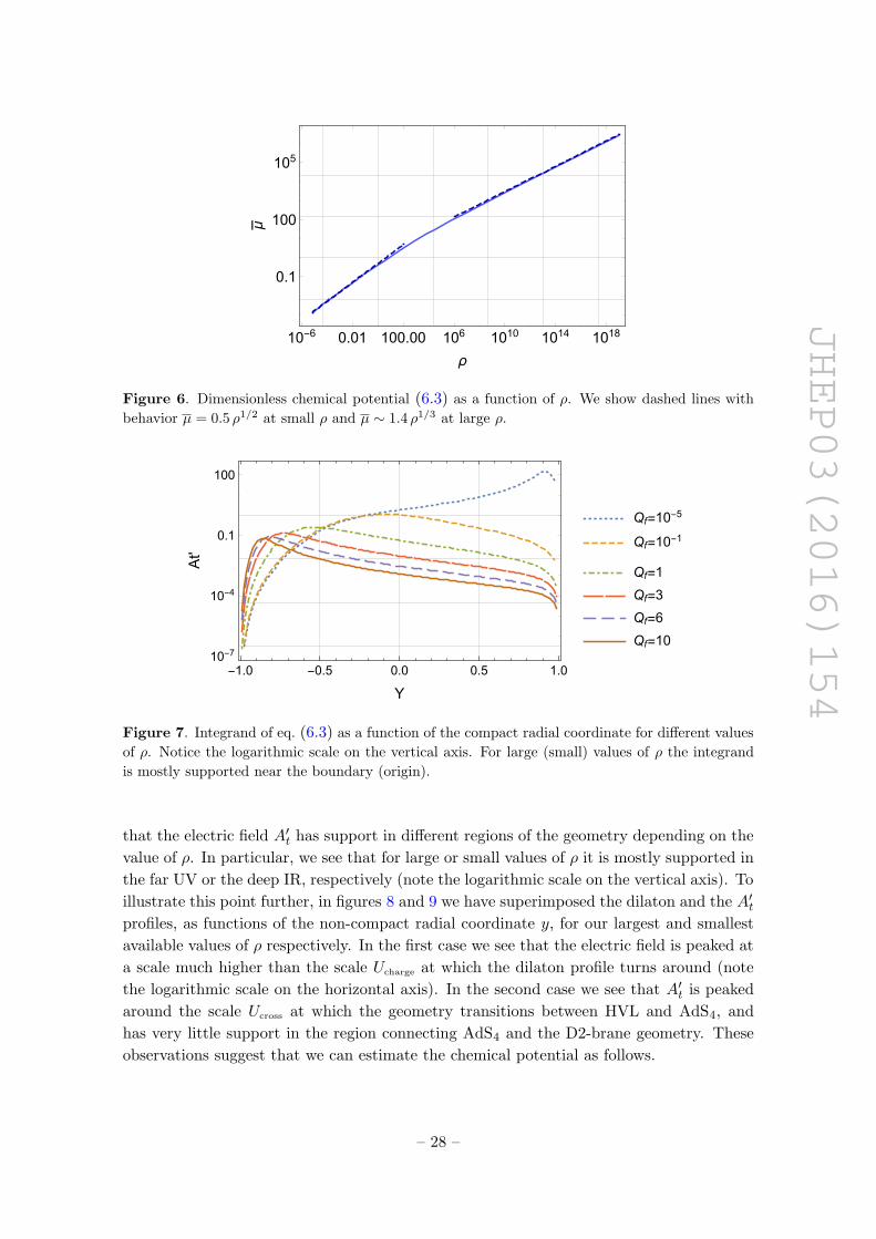
Figure 6. Dimensionless chemical potential (6.3) as a function of ρ. We show dashed lines with
behavior µ = 0.5 ρ1/2 at small ρ and µ ∼ 1.4 ρ1/3 at large ρ.
-1.0 -0.5 0.0 0.5 1.010-7
10-4
0.1
100
Y
At'
Qf=10-5
Qf=10-1
Qf=1
Qf=3
Qf=6
Qf=10
Figure 7. Integrand of eq. (6.3) as a function of the compact radial coordinate for different values
of ρ. Notice the logarithmic scale on the vertical axis. For large (small) values of ρ the integrand
is mostly supported near the boundary (origin).
that the electric field A′t has support in different regions of the geometry depending on the
value of ρ. In particular, we see that for large or small values of ρ it is mostly supported in
the far UV or the deep IR, respectively (note the logarithmic scale on the vertical axis). To
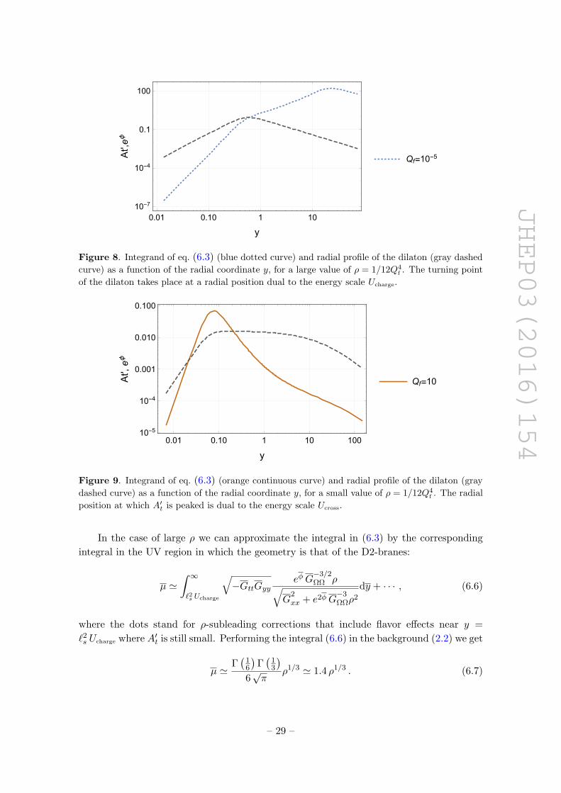
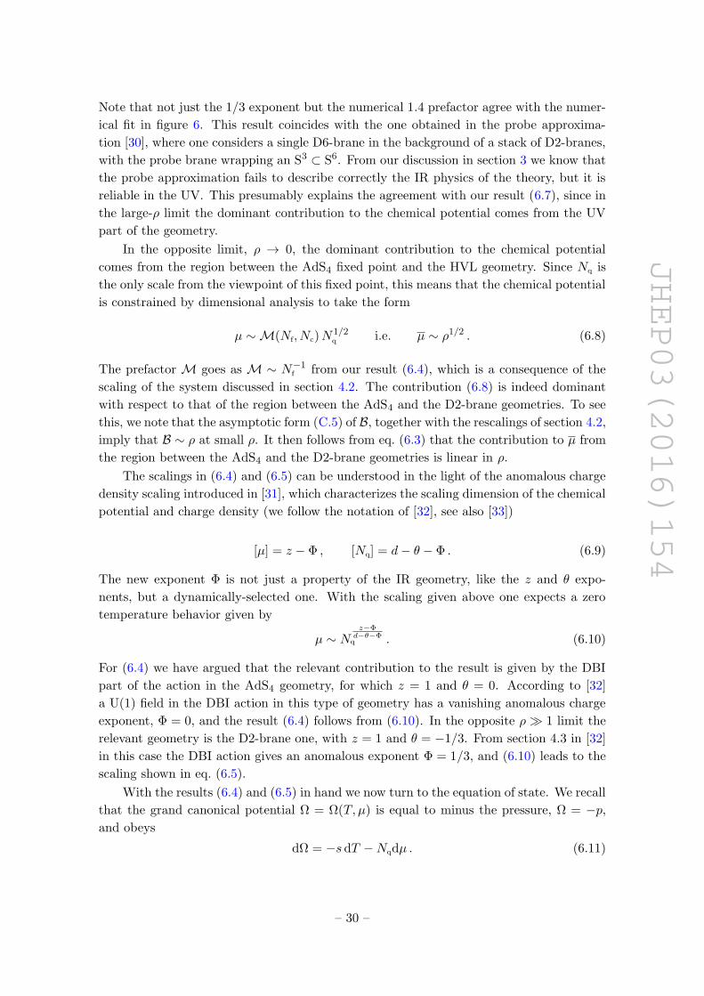
illustrate this point further, in figures 8 and 9 we have superimposed the dilaton and the A′tprofiles, as functions of the non-compact radial coordinate y, for our largest and smallest
available values of ρ respectively. In the first case we see that the electric field is peaked at
a scale much higher than the scale Ucharge at which the dilaton profile turns around (note
the logarithmic scale on the horizontal axis). In the second case we see that A′t is peaked
around the scale Ucross at which the geometry transitions between HVL and AdS4, and
has very little support in the region connecting AdS4 and the D2-brane geometry. These
observations suggest that we can estimate the chemical potential as follows.
– 28 –
JHEP03(2016)154
0.01 0.10 1 1010-7
10-4
0.1
100
y
At',eϕ
Qf=10-5
Figure 8. Integrand of eq. (6.3) (blue dotted curve) and radial profile of the dilaton (gray dashed
curve) as a function of the radial coordinate y, for a large value of ρ = 1/12Q4f . The turning point
of the dilaton takes place at a radial position dual to the energy scale Ucharge.
0.01 0.10 1 10 10010-5
10-4
0.001
0.010
0.100
y
At',eϕ
Qf=10
Figure 9. Integrand of eq. (6.3) (orange continuous curve) and radial profile of the dilaton (gray
dashed curve) as a function of the radial coordinate y, for a small value of ρ = 1/12Q4f . The radial
position at which A′t is peaked is dual to the energy scale Ucross.
In the case of large ρ we can approximate the integral in (6.3) by the corresponding
integral in the UV region in which the geometry is that of the D2-branes:
µ '∫ ∞`2s Ucharge
√−GttGyy
eφG−3/2ΩΩ ρ√
G2xx + e2φG
−3ΩΩρ
2
dy + · · · , (6.6)
where the dots stand for ρ-subleading corrections that include flavor effects near y =
`2s Ucharge where A′t is still small. Performing the integral (6.6) in the background (2.2) we get
µ 'Γ(
16
)Γ(
13
)6√π
ρ1/3 ' 1.4 ρ1/3 . (6.7)
– 29 –
JHEP03(2016)154
Note that not just the 1/3 exponent but the numerical 1.4 prefactor agree with the numer-
ical fit in figure 6. This result coincides with the one obtained in the probe approxima-
tion [30], where one considers a single D6-brane in the background of a stack of D2-branes,
with the probe brane wrapping an S3 ⊂ S6. From our discussion in section 3 we know that
the probe approximation fails to describe correctly the IR physics of the theory, but it is
reliable in the UV. This presumably explains the agreement with our result (6.7), since in
the large-ρ limit the dominant contribution to the chemical potential comes from the UV
part of the geometry.
In the opposite limit, ρ → 0, the dominant contribution to the chemical potential
comes from the region between the AdS4 fixed point and the HVL geometry. Since Nq is
the only scale from the viewpoint of this fixed point, this means that the chemical potential
is constrained by dimensional analysis to take the form
µ ∼M(Nf, Nc)N1/2q i.e. µ ∼ ρ1/2 . (6.8)
The prefactor M goes as M ∼ N−1f from our result (6.4), which is a consequence of the
scaling of the system discussed in section 4.2. The contribution (6.8) is indeed dominant
with respect to that of the region between the AdS4 and the D2-brane geometries. To see
this, we note that the asymptotic form (C.5) of B, together with the rescalings of section 4.2,
imply that B ∼ ρ at small ρ. It then follows from eq. (6.3) that the contribution to µ from
the region between the AdS4 and the D2-brane geometries is linear in ρ.
The scalings in (6.4) and (6.5) can be understood in the light of the anomalous charge
density scaling introduced in [31], which characterizes the scaling dimension of the chemical
potential and charge density (we follow the notation of [32], see also [33])
[µ] = z − Φ , [Nq] = d− θ − Φ . (6.9)
The new exponent Φ is not just a property of the IR geometry, like the z and θ expo-
nents, but a dynamically-selected one. With the scaling given above one expects a zero
temperature behavior given by
µ ∼ Nz−Φd−θ−Φ
q . (6.10)
For (6.4) we have argued that the relevant contribution to the result is given by the DBI
part of the action in the AdS4 geometry, for which z = 1 and θ = 0. According to [32]
a U(1) field in the DBI action in this type of geometry has a vanishing anomalous charge
exponent, Φ = 0, and the result (6.4) follows from (6.10). In the opposite ρ 1 limit the
relevant geometry is the D2-brane one, with z = 1 and θ = −1/3. From section 4.3 in [32]
in this case the DBI action gives an anomalous exponent Φ = 1/3, and (6.10) leads to the
scaling shown in eq. (6.5).
With the results (6.4) and (6.5) in hand we now turn to the equation of state. We recall
that the grand canonical potential Ω = Ω(T, µ) is equal to minus the pressure, Ω = −p,and obeys
dΩ = −s dT −Nqdµ . (6.11)
– 30 –
JHEP03(2016)154
In contrast, the energy density is naturally a function ε(s,Nq) and obeys the first law of
thermodynamics
dε = T ds+ µ dNq . (6.12)
At zero temperature this relations imply that
dp
dε=Nq
µ
dµ
dNq=ρ
µ
dµ
dρ=ρ
µ
dµ
dρ. (6.13)
Consequently, for small values of ρ we find ε = 2p, while for large values we get ε =
3p + const. We thus see that the speed of sound, c2s = dp/dε, varies from the conformal
value c2s = 1/2 at small ρ to c2
s = 1/3 at large ρ.
The fact that the chemical potential is a monotonically increasing function of the
charge density, i.e. that∂µ
∂ρ> 0 , (6.14)
indicates that the system is locally thermodynamically stable against charge fluctuations.
6.2 Entropy density at low temperature and IR degrees of freedom
We have seen that the IR geometry is always an HVL metric with fixed exponents z, θ
regardless of the values of λ,Nc, Nf and Nq that define the theory. This symmetry implies
that the entropy density at low temperatures must scale as in (1.8). However, the pro-
portionality coefficient in this equation, which measures the number of low-energy degrees
of freedom in the theory, does depend on λ,Nc, Nf and Nq. Following section 3.4 of [17],
in this section we will determine this dependence analytically for flows with very large or
very small ρ, and numerically for the rest of them. In the equations below we will omit
factors of `s, since they can be simply reinstated by dimensional analysis, as well as purely
numerical factors, since we are only interested in the parametric dependence of the entropy
density on λ,Nc, Nf and Nq.
It is straightforward to construct the non-zero-temperature generalization of the HVL
solution (2.8), which is a black hole with horizon radius rH whose explicit form is given in
section 3.2 of [17]. With this solution in hand one can compute the entropy density at low
temperature from the area of the horizon. The result is
s ∼ N2c
λ3/2U
7/2T , (6.15)
with UT the scale associated to the radius of the horizon via the relation (2.13). The
temperature is obtained from the Einstein-frame metric, GE, as
T ∼ ∂r(−GEtt)√
−GEttG
Err
∣∣∣∣∣r→rH
∼√Ct Nc U
35/2T
λ43/10N1/2q
. (6.16)
Using (6.16) to eliminate UT and substituting in (6.15) we find
s ∼ C−1/10t λ−16/25N2
c
(Nq
N2c
)1/10
T 1/5 . (6.17)
– 31 –
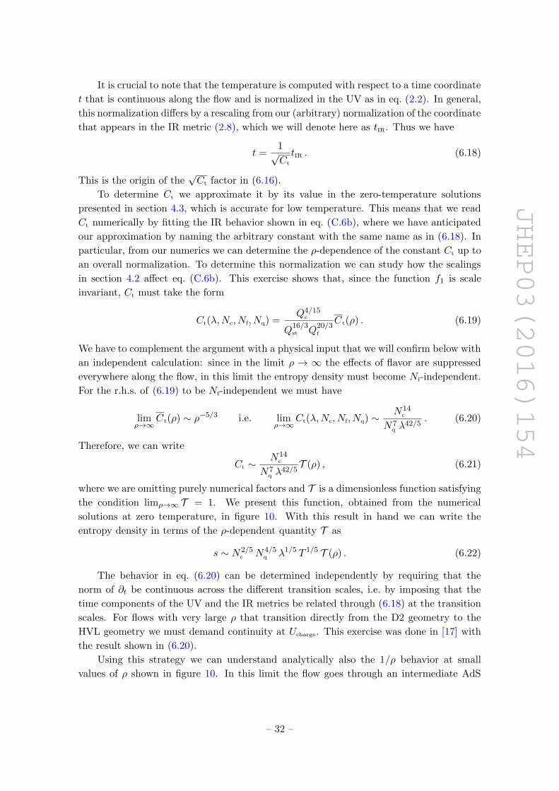
JHEP03(2016)154
It is crucial to note that the temperature is computed with respect to a time coordinate
t that is continuous along the flow and is normalized in the UV as in eq. (2.2). In general,
this normalization differs by a rescaling from our (arbitrary) normalization of the coordinate
that appears in the IR metric (2.8), which we will denote here as tIR. Thus we have
t =1√Ct
tIR . (6.18)
This is the origin of the√Ct factor in (6.16).
To determine Ct we approximate it by its value in the zero-temperature solutions
presented in section 4.3, which is accurate for low temperature. This means that we read
Ct numerically by fitting the IR behavior shown in eq. (C.6b), where we have anticipated
our approximation by naming the arbitrary constant with the same name as in (6.18). In
particular, from our numerics we can determine the ρ-dependence of the constant Ct up to
an overall normalization. To determine this normalization we can study how the scalings
in section 4.2 affect eq. (C.6b). This exercise shows that, since the function f1 is scale
invariant, Ct must take the form
Ct(λ,Nc, Nf, Nq) =Q4/15
c
Q16/3st Q
20/3f
Ct(ρ) . (6.19)
We have to complement the argument with a physical input that we will confirm below with
an independent calculation: since in the limit ρ → ∞ the effects of flavor are suppressed
everywhere along the flow, in this limit the entropy density must become Nf-independent.
For the r.h.s. of (6.19) to be Nf-independent we must have
limρ→∞
Ct(ρ) ∼ ρ−5/3 i.e. limρ→∞
Ct(λ,Nc, Nf, Nq) ∼ N14c
N7q λ
42/5. (6.20)
Therefore, we can write
Ct ∼N14
c
N7q λ
42/5T (ρ) , (6.21)
where we are omitting purely numerical factors and T is a dimensionless function satisfying
the condition limρ→∞ T = 1. We present this function, obtained from the numerical
solutions at zero temperature, in figure 10. With this result in hand we can write the
entropy density in terms of the ρ-dependent quantity T as
s ∼ N2/5c N4/5
q λ1/5 T 1/5 T (ρ) . (6.22)
The behavior in eq. (6.20) can be determined independently by requiring that the
norm of ∂t be continuous across the different transition scales, i.e. by imposing that the
time components of the UV and the IR metrics be related through (6.18) at the transition
scales. For flows with very large ρ that transition directly from the D2 geometry to the
HVL geometry we must demand continuity at Ucharge. This exercise was done in [17] with
the result shown in (6.20).
Using this strategy we can understand analytically also the 1/ρ behavior at small
values of ρ shown in figure 10. In this limit the flow goes through an intermediate AdS
– 32 –
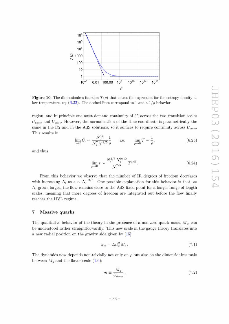
JHEP03(2016)154
10-6 0.01 100.00 106 1010 1014 10181
10
100
1000
104
105
106
ρ
(ρ)
Figure 10. The dimensionless function T (ρ) that enters the expression for the entropy density at
low temperature, eq. (6.22). The dashed lines correspond to 1 and a 1/ρ behavior.
region, and in principle one must demand continuity of Ct across the two transition scales
Uflavor and Ucross. However, the normalization of the time coordinate is parametrically the
same in the D2 and in the AdS solutions, so it suffices to require continuity across Ucross.
This results in
limρ→0
Ct ∼N14
c
N7q λ
42/5
1
ρi.e. lim
ρ→0T ∼ 1
ρ, (6.23)
and thus
limρ→0
s ∼N3/5
c N9/10q
N2/5f
T 1/5 . (6.24)
From this behavior we observe that the number of IR degrees of freedom decreases
with increasing Nf as s ∼ N−2/5f . One possible explanation for this behavior is that, as
Nf grows larger, the flow remains close to the AdS fixed point for a longer range of length
scales, meaning that more degrees of freedom are integrated out before the flow finally
reaches the HVL regime.
7 Massive quarks
The qualitative behavior of the theory in the presence of a non-zero quark mass, Mq, can
be understood rather straightforwardly. This new scale in the gauge theory translates into
a new radial position on the gravity side given by [15]
uM = 2π`2sMq . (7.1)
The dynamics now depends non-trivially not only on ρ but also on the dimensionless ratio
between Mq and the flavor scale (1.6):
m ≡ Mq
Uflavor
. (7.2)
– 33 –
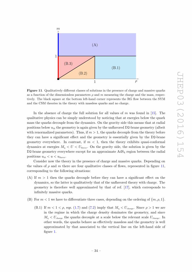
JHEP03(2016)154
(B.1)
(A)
(B.2)
(B.3)
1
1
ρ
m
Figure 11. Qualitatively different classes of solutions in the presence of charge and massive quarks
as a function of the dimensionless parameters ρ and m measuring the charge and the mass, respec-
tively. The black square at the bottom left-hand corner represents the RG flow between the SYM
and the CSM theories in the theory with massless quarks and no charge.
In the absence of charge the full solution for all values of m was found in [15]. The
qualitative physics can be simply understood by noticing that at energies below the quark
mass the quarks decouple from the dynamics. On the gravity side this means that at radial
positions below uM the geometry is again given by the unflavored D2-brane geometry (albeit
with renormalized parameters). Thus, if m > 1, the quarks decouple from the theory before
they can have a significant effect and the geometry is essentially given by the D2-brane
geometry everywhere. In contrast, if m < 1, then the theory exhibits quasi-conformal
dynamics at energies Mq < U < Uflavor. On the gravity side, the solution is given by the
D2-brane geometry everywhere except for an approximate AdS4 region between the radial
positions uM < u < uflavor.
Consider now the theory in the presence of charge and massive quarks. Depending on
the values of ρ and m there are four qualitative classes of flows, represented in figure 11,
corresponding to the following situations:
(A) If m > 1 then the quarks decouple before they can have a significant effect on the
dynamics, so the latter is qualitatively that of the unflavored theory with charge. The
geometry is therefore well approximated by that of ref. [17], which corresponds to
infinitely massive quarks.
(B) For m < 1 we have to differentiate three cases, depending on the ordering of m, ρ, 1.
(B.1) If m < 1 < ρ, eqs. (1.7) and (7.2) imply that Mq < Ucharge. Since ρ > 1 we are
in the regime in which the charge density dominates the geometry, and since
Mq < Ucharge the quarks decouple at a scale below the relevant scale Ucharge. In
other words, the quarks behave as effectively massless and the geometry is well
approximated by that associated to the vertical line on the left-hand side of
figure 1.
– 34 –
JHEP03(2016)154
(B.2) For m < ρ < 1, eqs. (1.7), (1.10) and (7.2) imply that Mq < Ucross. Since ρ < 1
we are in the regime in which the flow is close to the right-hand side of the
triangle of figure 1, and since Mq < Ucross the quarks decouple at a scale below
the lowest relevant scale Ucross. In other words, the quarks behave as effectively
massless and the geometry is well approximated by one of the flows with an
intermediate AdS4 region on the right-hand side of figure 1.
(B.3) Finally, consider the case in which ρ < m < 1 in such a way that Ucross < Mq <
Uflavor. The flow starts off in the UV with the D2-brane geometry, exhibits an
AdS4 region at energy scales Mq < U < Uflavor, becomes again well approximated
by the D2-brane geometry at energy scales U ′cross < U < Mq, and finally enters
a charge-dominated HVL region at energies U < U ′cross. The coupling constant
in the second D2 region is renormalized with respect to the UV coupling due to
the integrating out of the quarks and (omitting some purely numerical factors)
is given by [15]
λ′ ∼(
1 +1
m
)λ . (7.3)
Correspondingly, the scale U ′cross is given by (1.4) with the replacement λ→ λ′,
i.e.
U ′cross ∼√λ′(Nq
N2c
)1/4
∼M1/2q
(Nq
N2f
)1/4
, (7.4)
where the last expression is valid if m is sufficiently smaller than 1.
Acknowledgments
We thank Aristomenis Donos, Pau Figueras, Matti Jarvinen, Prem Kumar, Wilke van der
Schee, Miquel Triana and Miguel Zilhao for discussions. We are grateful to the Galileo
Galilei Institute in Florence (AF, CP, JT), to the Centro de Ciencias de Benasque Pedro
Pascual (AF, DM, CP, JT), to the Physics Departament at the University of California,
Santa Barbara (DM), and to the Institute for Nuclear Theory, University of Washington
(DM), for hospitality during part of this work. We are supported by grants 2014-SGR-
1474, MEC FPA2013-46570-C2-1-P, MEC FPA2013- 46570-C2-2-P, CPAN CSD2007-00042
Consolider-Ingenio 2010, ERC Starting Grant HoloLHC-306605 and Maria de Maeztu Unit
of Research Excellence distinction. JT is also supported by the Juan de la Cierva program
of the Spanish Ministry of Economy, by the Advanced ARC project “Holography, Gauge
Theories and Quantum Gravity” and by the Belgian Fonds National de la Recherche Scien-
tifique FNRS (convention IISN 4.4503.15). AK is supported by the Department of Atomic
Energy, Govt. of India. He is also grateful for the warm hospitality at the University of
Barcelona during the final stages of this work.
– 35 –
JHEP03(2016)154
A Supergravity with sources
In this appendix we will derive the equations of motion that we have solved in the main
part of the paper. Our starting point is the type IIA supergravity action. This is the sum
of a Neveu-Schwarz (NS) and a Ramond-Ramond (RR) sector,
SIIA = SNS + SRR , (A.1)
respectively given by
SNS =1
2κ2
∫e−2φ
(R ∗ 1 + 4 dφ ∧ ∗dφ− 1
2H ∧ ∗H
), (A.2a)
SRR =1
2κ2
1
2
∫(−G2 ∧ ∗G2 −G4 ∧ ∗G4 +H ∧ C3 ∧ dC3) , (A.2b)
where the field strengths are defined as
G2 = dC1 , G4 = dC3 −H ∧ C1 , H = dB . (A.3)
The equations of motion that follow from this action for the NS and RR forms are
d ∗G2 = −H ∧ ∗G4 , (A.4a)
d ∗G4 = −H ∧G4 , (A.4b)
d(e−2φ ∗H
)= G2 ∧ ∗G4 +
1
2G4 ∧G4 . (A.4c)
Note that in order to write the topological G4 ∧G4 term in the last equation in this form
one must use (A.4b).
We will now consider the addition of electric and magnetic sources for C1 and C3. For
this purpose it is convenient to use the so-called ‘democratic formulation’ [34] in which
the Hodge duals of these potentials are treated as independent fields, thus making all
the sources purely electric and hence mutually independent. The democratic formulation
provides a pseudo-action instead of an action in the sense that the duality relations between
Hodge potentials must be imposed by hand after obtaining the equations of motion. In
this formulation the RR part of the action is replaced by
SdemocraticRR =
1
2κ2
1
2
∫ (−1
2G2 ∧ ∗G2 −
1
2G4 ∧ ∗G4 −
1
2G6 ∧ ∗G6 −
1
2G8 ∧ ∗G8
), (A.5)
where the extra factors of 1/2 account for the doubling of the degrees of freedom. The field
strengths are defined as
Gn = dCn−1 −H ∧ Cn−3 (A.6)
with n = 2, 4, 6, 8 and C−1 = 0. The equations of motion that follow from the new pseudo-
action for the RR fields are
d ∗G8 = 0 , (A.7a)
d ∗G6 = −H ∧ ∗G8 , (A.7b)
d ∗G4 = −H ∧ ∗G6 , (A.7c)
d ∗G2 = −H ∧ ∗G4 , (A.7d)
– 36 –
JHEP03(2016)154
whereas the equation for the H-field is
d(e−2φ ∗H
)=
1
2d(C1 ∧ ∗G4 + C3 ∧ ∗G6 + C5 ∧ ∗G8
)=
1
2G2 ∧ ∗G4 +
1
2G4 ∧ ∗G6 +
1
2G6 ∧ ∗G8 . (A.8)
Note that in order to obtain this last equation one must make use of (A.7). The duality
equations that must be imposed after the equations of motion have been obtained are
G8 = ∗G2 G6 = − ∗G4 , (A.9)
where ∗∗ = −1 for even forms. By means of these duality relations one may turn the
equations of motion (A.7) into the set of Bianchi identities
dGn = H ∧Gn−2 , (A.10)
which are explicitly solved by the definitions (A.6) in terms of gauge potentials.
We now consider the addition of smeared D6-branes with an arbitrary worldvolume
gauge field turned on. The action for the D6-branes is the sum of a Dirac-Born-Infeld
(DBI) term and a Wess-Zumino (WZ) term:
SD6 = SDBI + SWZ . (A.11)
In the following we will only need the explicit form of the WZ term:
SWZ =1
2κ2
∫1
2
(C7 − C5 ∧ F +
1
2C3 ∧ F ∧ F −
1
6C1 ∧ F ∧ F ∧ F
)∧ Γ . (A.12)
As above, the overall factor of 1/2 is due to the doubling of degrees of freedom. We
have absorbed the brane tension in the definition of Γ, which is a closed three-form that
characterizes the distribution of D6-branes in the codimension-three space transverse to
them. For example, for a single brane located at a particular point, specified by three
coordinates ζD6, one would have
Γ ∼ δ3(ζ − ζD6) dζ1 ∧ dζ2 ∧ dζ3 . (A.13)
The field strength appearing in the WZ action is
F = B + 2π`2s dA , (A.14)
where A is the Born-Infeld field living on the worldvolume of the D6-branes, and it satisfies
the Bianchi identity
dF = H . (A.15)
The WZ term acts as a source for both the RR fields and the H-field, and hence it
modifies their equations of motion. For the RR fields, we will see that, through the duality
relations, this also leads to a modification of their Bianchi identities, and therefore to a
modification of their very definition in terms of gauge potentials. For this reason we write
– 37 –
JHEP03(2016)154
the modified equations of motion in terms of new RR field strengths that we denote Fn.
The equations for these RR fields read
d ∗ F8 = Γ , (A.16a)
d ∗ F6 = −H ∧ ∗F8 −F ∧ Γ , (A.16b)
d ∗ F4 = −H ∧ ∗F6 +1
2F ∧ F ∧ Γ , (A.16c)
d ∗ F2 = −H ∧ ∗F4 −1
6F ∧ F ∧ F ∧ Γ . (A.16d)
Apart from the change of notation Gn → Fn, these are just equations (A.7) augmented
with the extra source terms coming from the variation of (A.12). We now see that in order
to impose duality relations analogous to (A.9), namely
F8 = ∗F2 F6 = − ∗ F4 , (A.17)
we must modify the definitions of the RR field strengths with respect to those in (A.6).
For example, upon use of (A.17), the first equation in (A.16) reads
dF2 = −Γ , (A.18)
which is obviously incompatible with F2 = dC1. This problem is familiar from electro-
magnetism when both electric and magnetic sources are simultaneously present. In such a
situation, in order to be able to define a gauge potential, one must modify the definition of
the electric and magnetic fields in terms of this potential. In our case, the set of Bianchi
identities that is obtained by using (A.17) in (A.16) is solved by the definitions
F2 = G2 + γ , (A.19a)
F4 = G4 + F ∧ γ , (A.19b)
F6 = G6 +1
2F ∧ F ∧ γ , (A.19c)
F8 = G8 +1
6F ∧ F ∧ F ∧ γ , (A.19d)
where Gn are defined as in (A.6) and γ is a two-form satisfying
dγ = −Γ . (A.20)
Note that γ always exists locally because Γ is closed.
The equation of motion for H is (A.8) augmented by contributions from both the D6-
brane action and the definitions (A.19). Upon the replacement Gn → Fn in the action,
and taking into account the DBI and WZ terms this equation is now
d(e−2φ ∗H
)=
1
2d (C1 ∧ ∗F4 + C3 ∧ ∗F6 + C5 ∧ ∗F8) (A.21)
+1
2
(∗F4 + F ∧ ∗F6 +
1
2F ∧ F ∧ ∗F8
)∧ γ
+1
2
(C5 −F ∧ C3 +
1
2F ∧ F ∧ C1
)∧ Γ
+ DBI-terms.
– 38 –
JHEP03(2016)154
Using (A.19) and the equations of motion (A.16), the equation for the H-field can be simply
written as
d(e−2φ ∗H
)=
1
2F2 ∧ ∗F4 +
1
2F4 ∧ ∗F6 +
1
2F6 ∧ ∗F8
+ DBI-terms . (A.22)
It is possible to write down the RR part of the supergravity action and the WZ term of
the D6-brane action directly in terms of the modified field strengths Fn. In the democratic
formulation these are given by
SdemocraticRR = − 1
2κ2
1
2
∫ (1
2F2 ∧ ∗F2 +
1
2F4 ∧ ∗F4 +
1
2F6 ∧ ∗F6 −
1
2F8 ∧ ∗F8
), (A.23)
SWZ = − 1
2κ2
1
2
∫ (F8 − F6 ∧ F +
1
2F4 ∧ F ∧ F −
1
6F2 ∧ F ∧ F ∧ F
)∧ γ . (A.24)
We finally return to the non-democratic formulation and note that, in the presence of
sources, the RR part of the supergravity action and the WZ term of the D6-brane action
can be written directly in terms of the modified field strengths F2 and F4 alone:
SRR = − 1
2κ2
1
2
∫ (F2 ∧ ∗F2 + F4 ∧ ∗F4 −
1
2H ∧ C3 ∧ dC3
), (A.25)
SWZ = − 1
2κ2
∫ (1
2F4 ∧ F ∧ F −
1
6F2 ∧ F ∧ F ∧ F −
1
6F ∧ F ∧ F ∧ γ
)∧ γ . (A.26)
By varying the resulting complete action with respect to the dilaton, the metric and the
RR and NS potentials, one obtains complete set of equations that we have solved in this
paper and which we collect here. The equations of motion for the RR and NS forms are
d ∗ F4 = −H ∧ F4 +1
2F ∧ F ∧ Γ , (A.27a)
d ∗ F2 = −H ∧ ∗F4 −1
6F ∧ F ∧ F ∧ Γ , (A.27b)
d(e−2φ ∗H
)= F2 ∧ ∗F4 +
1
2F4 ∧ F4 + DBI-term . (A.27c)
Since the gauge field A living in the worldvolume of the D6-branes can be seen as a
Stuckelberg vector field for the NS two-form B, the equation of motion for A follows from
the equation of motion for B and it takes the form
d
[F2 ∧ ∗F4 +
1
2F4 ∧ F4 + DBI-terms
]= 0 . (A.28)
The equation of motion for the dilaton is given by
R ∗ 1 + 4d ∗ dφ− 6dφ ∧ ∗dφ− 1
2H ∧ ∗H + DBI-terms = 0 (A.29)
Finally, the Einstein equations read
Rµν = −2∇µ∇νφ+1
4HµρσHν
ρσ (A.30)
+ e2φ
[1
2(F2)µρ (F2)ν
ρ +1
12(F4)µρσα (F4)ν
ρσα − 1
4Gµν (F2yF2 + F4yF4)
]+ DBI-terms ,
– 39 –
JHEP03(2016)154
where for any two n-forms ω, ξ we have defined
ωyξ =1
n!ωM1...Mnξ
M1...Mn . (A.31)
In the bulk of the paper we have written
Γ = 2κ2 TD6 Ξ , γ = Qf J . (A.32)
B Equations of motion
In this section we will write down explicitly the full set of equations of motion for the
overlined variables introduced in section 4.2. Eq. (4.24) for the time component of the U(1)
vector field takes the form (4.36) in terms of these variables. This could be substituted
in the remaining equations to eliminate the dependence on A′t. However, we will follow
the alternative route of eliminating A′t at the level of the action by performing a Legendre
transform that modifies the contribution of the sources in (4.1) to
Ssources−∫∂Ssources
∂A′tA′t = − Q
5f
2κ2
∫e−φG
−3/2ΩΩ
√√√√1 +
(eφ(ρ+ B)
GxxG3/2ΩΩ
)2
∗1+TD6
∫C7∧Ξ . (B.1)
To arrive at (B.1) we have explicitly used the fact that the NSNS form vanishes, B = 0.
Otherwise there would be an extra term proportional to Byt, coming from the coupling in
the WZ part of the D6-action between B and and the worldvolume gauge field, A. In our
case it is consistent to set B = 0 in the action at this stage because the sourcing due to
the strings has already been taken into consideration explicitly.
After elimination of A′t, the equations of motion take the following form. The equation
for the function B appearing in the RR fluxes is
∂y
(√−GttGyy
B′
Gxx
)− 12
√−GttGyyGxxGΩΩ
B −3 eφ
√−GttGyy (ρ+ B)√
G2xxG
3ΩΩ + e2φ (ρ+ B)2
= 0 . (B.2)
The dilaton equation of motion becomes
0 = φ′′ + log′
[e−2φ
√−GttGxxG3
ΩΩ√Gyy
]φ′ +
e2φ B′2
G2xxG
3ΩΩ
+1
2F1,−9,−3,3(y) (B.3)
− 3 eφGyy
(3G2
xxG3ΩΩ + 2 e2φ (ρ+ B)2
)GxxG3
ΩΩ
√G2xxG
3ΩΩ + e2φ (ρ+ B)2
,
where for notational convenience we have defined
FA,B,C,D(y) = e2φ Gyy2G2
xxG6ΩΩ
[G2xx
(A+BG4
ΩΩ
)+ 16G2
ΩΩ
(9C ρ2G4
ΩΩ +DB2) ]. (B.4)
– 40 –
JHEP03(2016)154
Finally, Einstein equations reduce to the following set of second order differential equations
0 = G′′tt + log′
[e−2φ GxxG
3ΩΩ√
−GttGyy
]G′tt +
(2 e2φ B′2
G2xxG
3ΩΩ
−F1,3,1,3(y)
)Gtt (B.5a)
− 6 eφGyy Gtt
(G2xxG
3ΩΩ + 2 e2φ (ρ+ B)2
)GxxG3
ΩΩ
√G2xxG
3ΩΩ + e2φ (ρ+ B)2
,
0 = G′′xx + log′
[e−2φ
√−GttG3
ΩΩ√Gyy
]G′xx +
(2 e2φ B′2
G2xxG
3ΩΩ
+ F−1,−3,1,3(y)
)Gxx (B.5b)
− 6 eφGyy G
2xx√
G2xxG
3ΩΩ + e2φ (ρ+ B)2
,
0 = G′′ΩΩ + log′
[e−2φ
√−GttGxxG2
ΩΩ√Gyy
]G′ΩΩ + F1,−1,−1,1(y)GΩΩ − 10Gyy , (B.5c)
together with the first order constraint
0 = φ′ log′[e−φ√−GttGxxG3
ΩΩ
]+ log′
[G−3/2ΩΩ
]log′
[√−GttGxxG5/4
ΩΩ
](B.6)
+ log′[G−1/2xx
]log′
[√−GttG1/4
xx
]+
e2φ B′2
2G2xxG
3ΩΩ
+15
2
GyyGΩΩ
− 1
4F1,3,1,3(y)
− 3eφGyyGxxG3
ΩΩ
√G2xxG
3ΩΩ + e2φ (ρ+ B)2 .
An effective one-dimensional Lagrangian giving rise to these equations of motion can be
derived from the constraint as
Leff = H −∑i
ψ′i∂H
∂ψ′i, (B.7)
with ψi running over all fields and H the r.h.s. of (B.6).
C Numerical construction of solutions
With the ansatz (4.38) the equation of motion for f2 can be solved algebraically with
the result
f2 =e−4χf1 g
2(−1500e4χy8 + 50Z e6χy4 g + (e12χQ2cQ
2st + 75e8χQ2
f y6 + 625y8 + 1200e4χy2B2)g2)
25y4(y5gf ′1(4yg′ − 7g) + f1(4g4B′2 + 38y5gg′ − 8y6g′2 + y4g2(−35− 6yχ′ + 12y2χ′2)))),
(C.1)
where we have defined
Z2 = 144Q2f y
6 + (QcQst + 12QfB)2g2 . (C.2)
The gauge field At on the D6-branes can be solved in terms of the other functions and is
given by
2πα′A′t =
√f1
f2
eχ(QcQst + 12QfB)g
Z. (C.3)
– 41 –
JHEP03(2016)154
The remaining functions obey the following set of four, coupled, second-order differential
equations
0 = B′′ + log′[√f1f2e
−χ]B′ − 12By2f2
−Qf
3 e2χ g (QcQst + 12QfB)
f2Z,
0 = g′′ − g3B′2
2y6+
1
2log′
[f2y
19/2
g4
]− 7
8
g
ylog′[y5f2e
−20χ/7]−χ′ (ge3χ/2)′
e3χ/2+
15g
2y2f2− g
2e2χZ4y6f2
− g3 e−4χ
200 y10 f2(625 y8 + 1200 y2 e4χB2 +Q2
cQ2st e
12χ + 75 y6Q2f e
8χ)
0 = χ′′ − 1
2log′
[f1 f2
g4
]log′[y1/4e−χ]− χ′2 − 5
4 ylog′[y e−5χ]− 5
y2f2
+g2 e−4χ
100 y10 f2(625 y8 + 400 y2 e4χB2 −Q2
cQ2st e
12χ − 25 y6Q2f e
8χ)
0 = f ′′1 − f ′1 log′[y−29/4 f1/21 eχ] +
(y5/2f1)′
2 y5/2log′
[f2
g4
]− g f1 e
2χ
y6 f2Z(Z2 − 72Q2
f y6)− 5 f1
2 yχ′
− 2g2f1
y6B′2+
25f1
2y2− g
2f1e−4χ
50y10f2(625y8+1200y2e4χB2+Q2
cQ2ste
12χ+75y6Q2f e
8χ) (C.4)
The boundary conditions that must be imposed are as follows. In the UV, as y →∞,
we demand that we have the asymptotic behavior given by
B =Qc Qst
Qf
(0− 1
40
Qf
y+
41
400
Q2f
y2+ B3
Q3f
y3+ · · ·+ log
[Qf
y
](143
840
Q3f
y3+ · · ·
)), (C.5a)
f1 = 1 + V1Q5
f
y5+ · · ·+ log
[Qf
y
](−143Q2
cQ2st
42000
Q2f
y10+ · · ·
), (C.5b)
g = 1− 13
10
Qf
y+ · · ·+ V2
Q5f
y5+ · · ·+ log
[Qf
y
](−143Q2
cQ2st
120000
Q2f
y10+ · · ·
), (C.5c)
χ = 0− 17
30
Qf
y+ · · ·+ V3
Q10f
y10+ · · ·+ log
[Qf
y
](5291Q2
cQ2st
2520000
Q2f
y10+ · · ·
), (C.5d)
The most important thing to notice is that this implies that the solution approaches the
D2-brane solution (2.2). The expansion (C.5) is specified by four dimensionless parameters
B3, V1, V2 and V3 holographically dual to the expectation values of the operators dual to
B, the stress tensor, TrF 2 and TrF 4 respectively.
In the IR, as y → 0, we demand that the fields approach their values in the HVL
solution (2.8). In the radial coordinate that we have chosen this implies the following
– 42 –
JHEP03(2016)154
expansion
B = CB y∆3 − 3 · 52/3Qf
(14QcQst)1/3y10/3 + · · · , (C.6a)
f1 = Ct
Q16/3st
Q4/15c
y20/3
(1 +
1
11(87 +
√793)c1 y
∆1 +1
11(87−
√793)c2 y
∆2 + · · ·), (C.6b)
g =51/6142/3
111/2(QcQst)1/3y4/3
(1+
1
22(21+
√793)c1y
∆1 +1
22(21−
√793)c2y
∆2 + · · ·), (C.6c)
eχ =101/3
(7QcQst)1/6y2/3
(1 + c1 y
∆1 + c2 y∆2 + · · ·
). (C.6d)
where we have reabsorbed a purely numeric factor in Ct with respect to the one in (2.8) and
∆1 =5
6
(−3 +
√3
11(381− 4
√793)
)(C.7)
∆2 =5
6
(−3 +
√3
11(381 + 4
√793)
)(C.8)
∆3 =5
6
(−1 +
√149
5
). (C.9)
Note that the IR expansion is completely determined in terms of four constants c1, c2, Ct
and CB.
The modes labelled by the powers ∆1,2 arise from the fluctuations of the metric and
the dilaton, and have appeared already in [17]. There it is explained that there exist
companion modes dual to relevant deformations (which we set to vanish in our solutions),
characterized by powers ∆1,2 satisfying the relation
∆1,2 + ∆1,2 = −5
6(p+ z − θ) (C.10)
with p = 2, z = 5 and θ = 1 in our case. The factor 5/6 appears because we work with the
y radial coordinate, in which the metric does not take the standard HV-Lifshitz form given
in eq. (1.1). In [17] it is shown that there is an additional deformation of the metric due
to the possibility of adding a temperature to the system. We have set it to zero to ensure
that the system remains at zero temperature. The third power in the IR expansion, ∆3,
appears only for the fluctuation of the function B, and comes accompanied by a relevant
deformation (which we set to zero) with a power ∆3 satisfying the relation
∆3 + ∆3 = −5
6(p+ z − θ − 4) (C.11)
as this function corresponds to a two-form in Minkowski spacetime (see eq. (4.15)).
D Spectrum of fluctuations around AdS4
In this appendix we will compute the spectrum of fluctuations around the AdS4 fixed point
present in figure 1. Using the standard AdS/CFT dictionary this will allow us to find the
dimension of the dual operators in the gauge theory.
– 43 –
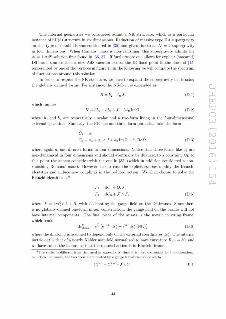
JHEP03(2016)154
The internal geometries we considered admit a NK structure, which is a particular
instance of SU(3) structure in six dimensions. Reduction of massive type IIA supergravity
on this type of manifolds was considered in [35] and gives rise to an N = 2 supergravity
in four dimensions. When Romans’ mass is non-vanishing, this supergravity admits the
N = 1 AdS solution first found in [36, 37]. If furthermore one allows for explicit (smeared)
D6-brane sources then a new AdS vacuum exists: the IR fixed point in the flows of [15]
represented by one of the vertices in figure 1. In the following we will compute the spectrum
of fluctuations around this solution.
In order to respect the NK structure, we have to expand the supergravity fields using
the globally defined forms. For instance, the NS-form is expanded as
B = b2 + b0 J , (D.1)
which implies
H = db2 + db0 ∧ J + 3 b0 Im Ω , (D.2)
where b0 and b2 are respectively a scalar and a two-form living in the four-dimensional
external spacetime. Similarly, the RR one and three-form potentials take the form
C1 = a1 ,
C3 = a3 + a1 ∧ J + a0 Im Ω + a0 Re Ω , (D.3)
where again ai and ai are i-forms in four dimensions. Notice that three-forms like a3 are
non-dynamical in four dimensions and should eventually be dualized to a constant. Up to
this point the ansatz coincides with the one in [35] (which in addition considered a non-
vanishing Romans’ mass). However, in our case the explicit sources modify the Bianchi
identities and induce new couplings in the reduced action. We then choose to solve the
Bianchi identities as6
F2 = dC1 +Qf J ,
F4 = dC3 + F ∧ F2 , (D.5)
where F = 2π`2s dA + B, with A denoting the gauge field on the D6-branes. Since there
is no globally-defined one-form in our construction, the gauge field on the branes will not
have internal components. The final piece of the ansatz is the metric in string frame,
which reads
ds2string = e
φ2(e−6U ds2
4 + e2U ds26 (NK)
)(D.6)
where the dilaton φ is assumed to depend only on the external coordinates ds24. The internal
metric ds26 is that of a nearly Kahler manifold normalized to have curvature RNK = 30, and
we have tuned the factors so that the reduced action is in Einstein frame.6This choice is different from that used in appendix A, since it is more convenient for the dimensional
reduction. Of course, the two choices are related by a gauge transformation given by
Cthere3 = Chere
3 + F ∧ C1 . (D.4)
– 44 –
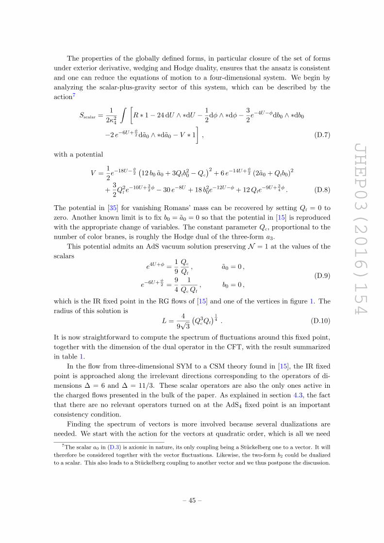
JHEP03(2016)154
The properties of the globally defined forms, in particular closure of the set of forms
under exterior derivative, wedging and Hodge duality, ensures that the ansatz is consistent
and one can reduce the equations of motion to a four-dimensional system. We begin by
analyzing the scalar-plus-gravity sector of this system, which can be described by the
action7
Sscalar =1
2κ24
∫ [R ∗ 1− 24 dU ∧ ∗dU − 1
2dφ ∧ ∗dφ− 3
2e−4U−φdb0 ∧ ∗db0
−2 e−6U+φ2 da0 ∧ ∗da0 − V ∗ 1
], (D.7)
with a potential
V =1
2e−18U−φ
2(12 b0 a0 + 3Qfb
20 −Qc
)2+ 6 e−14U+φ
2 (2a0 +Qfb0)2
+3
2Q2
f e−10U+ 3
2φ − 30 e−8U + 18 b20e
−12U−φ + 12Qfe−9U+ 3
4φ . (D.8)
The potential in [35] for vanishing Romans’ mass can be recovered by setting Qf = 0 to
zero. Another known limit is to fix b0 = a0 = 0 so that the potential in [15] is reproduced
with the appropriate change of variables. The constant parameter Qc, proportional to the
number of color branes, is roughly the Hodge dual of the three-form a3.
This potential admits an AdS vacuum solution preserving N = 1 at the values of the
scalars
e4U+φ =1
9
Qc
Qf
, a0 = 0 ,
e−6U+φ2 =
9
4
1
Qc Qf
, b0 = 0 ,
(D.9)
which is the IR fixed point in the RG flows of [15] and one of the vertices in figure 1. The
radius of this solution is
L =4
9√
3
(Q3
cQf
) 14 . (D.10)
It is now straightforward to compute the spectrum of fluctuations around this fixed point,
together with the dimension of the dual operator in the CFT, with the result summarized
in table 1.
In the flow from three-dimensional SYM to a CSM theory found in [15], the IR fixed
point is approached along the irrelevant directions corresponding to the operators of di-
mensions ∆ = 6 and ∆ = 11/3. These scalar operators are also the only ones active in
the charged flows presented in the bulk of the paper. As explained in section 4.3, the fact
that there are no relevant operators turned on at the AdS4 fixed point is an important
consistency condition.
Finding the spectrum of vectors is more involved because several dualizations are
needed. We start with the action for the vectors at quadratic order, which is all we need
7The scalar a0 in (D.3) is axionic in nature, its only coupling being a Stuckelberg one to a vector. It will
therefore be considered together with the vector fluctuations. Likewise, the two-form b2 could be dualized
to a scalar. This also leads to a Stuckelberg coupling to another vector and we thus postpone the discussion.
– 45 –
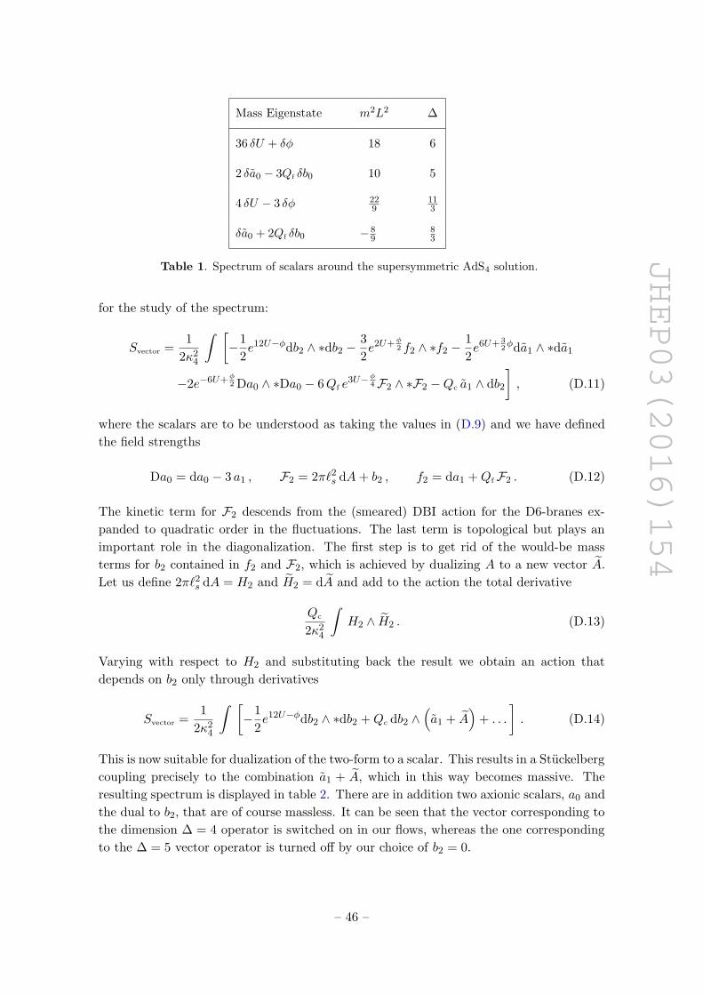
JHEP03(2016)154
Mass Eigenstate m2L2 ∆
36 δU + δφ 18 6
2 δa0 − 3Qf δb0 10 5
4 δU − 3 δφ 229
113
δa0 + 2Qf δb0 −89
83
Table 1. Spectrum of scalars around the supersymmetric AdS4 solution.
for the study of the spectrum:
Svector =1
2κ24
∫ [−1
2e12U−φdb2 ∧ ∗db2 −
3
2e2U+φ
2 f2 ∧ ∗f2 −1
2e6U+ 3
2φda1 ∧ ∗da1
−2e−6U+φ2 Da0 ∧ ∗Da0 − 6Qf e
3U−φ4F2 ∧ ∗F2 −Qc a1 ∧ db2
], (D.11)
where the scalars are to be understood as taking the values in (D.9) and we have defined
the field strengths
Da0 = da0 − 3 a1 , F2 = 2π`2s dA+ b2 , f2 = da1 +QfF2 . (D.12)
The kinetic term for F2 descends from the (smeared) DBI action for the D6-branes ex-
panded to quadratic order in the fluctuations. The last term is topological but plays an
important role in the diagonalization. The first step is to get rid of the would-be mass
terms for b2 contained in f2 and F2, which is achieved by dualizing A to a new vector A.
Let us define 2π`2s dA = H2 and H2 = dA and add to the action the total derivative
Qc
2κ24
∫H2 ∧ H2 . (D.13)
Varying with respect to H2 and substituting back the result we obtain an action that
depends on b2 only through derivatives
Svector =1
2κ24
∫ [−1
2e12U−φdb2 ∧ ∗db2 +Qc db2 ∧
(a1 + A
)+ . . .
]. (D.14)
This is now suitable for dualization of the two-form to a scalar. This results in a Stuckelberg
coupling precisely to the combination a1 + A, which in this way becomes massive. The
resulting spectrum is displayed in table 2. There are in addition two axionic scalars, a0 and
the dual to b2, that are of course massless. It can be seen that the vector corresponding to
the dimension ∆ = 4 operator is switched on in our flows, whereas the one corresponding
to the ∆ = 5 vector operator is turned off by our choice of b2 = 0.
– 46 –
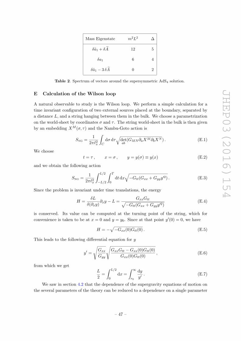
JHEP03(2016)154
Mass Eigenstate m2L2 ∆
δa1 + δA 12 5
δa1 6 4
δa1 − 3 δA 0 2
Table 2. Spectrum of vectors around the supersymmetric AdS4 solution.
E Calculation of the Wilson loop
A natural observable to study is the Wilson loop. We perform a simple calculation for a
time invariant configuration of two external sources placed at the boundary, separated by
a distance L, and a string hanging between them in the bulk. We choose a parametrization
on the world-sheet by coordinates σ and τ . The string world-sheet in the bulk is then given
by an embedding XM (σ, τ) and the Nambu-Goto action is
SNG =1
2π`2s
∫C
dσ dτ√
detab
(GMN∂aXM∂bXN ) . (E.1)
We choose
t = τ , x = σ , y = y(σ) ≡ y(x) (E.2)
and we obtain the following action
SNG =1
2π`2s
∫ L/2
−L/2
∫ T
0dt dx
√−Gtt(Gxx +Gyyy′2) . (E.3)
Since the problem is invariant under time translations, the energy
H =δL
δ(∂xy)∂xy − L =
GxxGtt√−Gtt(Gxx +Gyyy′2)
(E.4)
is conserved. Its value can be computed at the turning point of the string, which for
convenience is taken to be at x = 0 and y = y0. Since at that point y′(0) = 0, we have
H = −√−Gxx(0)Gtt(0) . (E.5)
This leads to the following differential equation for y
y′ =
√GxxGyy
√GxxGtt −Gxx(0)Gtt(0)
Gxx(0)Gtt(0), (E.6)
from which we getL
2=
∫ L/2
0dx =
∫ ∞r0
dy
y′. (E.7)
We saw in section 4.2 that the dependence of the supergravity equations of motion on
the several parameters of the theory can be reduced to a dependence on a single parameter
– 47 –
JHEP03(2016)154
ρ through the rescalings (4.32) and (4.34). In order to reduce the Nambu-Goto equations
of motion to the same dependence we must further rescale the x-coordinate as in eq. (5.1).
Under these circumstances the Nambu-Goto action scales homogeneously as SNG = Qf SNG.
One immediate consequence of (5.1) is that the distance between the endpoints of the
strings satisfies the same scaling property
L(λ,Nc, Nf, Nq) = Qf
(Qc
Q5f
)1/2
L(ρ) , (E.8)
and the energy of the system, which is evaluated by calculating the on-shell action divided
by the integral over time, can be expressed in terms of dimensionless variables as
E(λ,Nc, Nf, Nq) =S
T= Qf
S
T=
2Qf
2π`2s
∫ ∞y0
√−Gtt(Gxx +Gyyy′2)
dy
y′≡ Qf
2π`2sE(ρ) . (E.9)
The above quantity is divergent. The interpretation of this divergence is that we are really
computing the energy of a pair of quarks including their large self-energy. Since we are
only interested in the potential energy of the two sources, we subtract the energy of each
individual quark, corresponding to a string stretching all the way from y = 0 to y = ∞.
The final result is then given by
E = 2
(∫ ∞y0
√−Gtt(Gxx +Gyyy′2)
dy
y′−∫ ∞
0
√−GttGyy dy
). (E.10)
Applying the above procedure to the D2-brane solution we obtain
L ∼ y−3/20 , E ∼ y0 . (E.11)
In the case of AdS4, in the coordinate system used here, we get
L ∼ y−5/40 , E ∼ y5/4
0 . (E.12)
More precisely, using (E.10) and the rescaled version of (E.7) we have that the product
E · L in the AdS4 region is a constant given by (5.3). Finally, for the HVL geometry the
results are
L ∼ y−5/60 , E ∼ y5
0 . (E.13)
In figure 5, we have plotted the potential energy E in units of 1/L against the distance
between the two sources, L. We see that for small L, the Wilson loop is probing only the
UV part of the geometry and thus the energy scales as in the D2-brane solution. For large
L, the string penetrates deeper in the bulk, probing the IR region, and thus the scaling is
given by the HVL solution. At intermediate values of L, we see an AdS region building up.
Open Access. This article is distributed under the terms of the Creative Commons
Attribution License (CC-BY 4.0), which permits any use, distribution and reproduction in
any medium, provided the original author(s) and source are credited.
– 48 –
JHEP03(2016)154
References
[1] P. de Forcrand, Simulating QCD at finite density, PoS(LAT2009)010 [arXiv:1005.0539]
[INSPIRE].
[2] J.M. Maldacena, The large-N limit of superconformal field theories and supergravity, Int. J.
Theor. Phys. 38 (1999) 1113 [hep-th/9711200] [INSPIRE].
[3] S.S. Gubser, I.R. Klebanov and A.M. Polyakov, Gauge theory correlators from noncritical
string theory, Phys. Lett. B 428 (1998) 105 [hep-th/9802109] [INSPIRE].
[4] E. Witten, Anti-de Sitter space and holography, Adv. Theor. Math. Phys. 2 (1998) 253
[hep-th/9802150] [INSPIRE].
[5] D. Mateos, Gauge/string duality applied to heavy ion collisions: Limitations, insights and
prospects, J. Phys. G 38 (2011) 124030 [arXiv:1106.3295] [INSPIRE].
[6] J. Casalderrey-Solana, H. Liu, D. Mateos, K. Rajagopal and U.A. Wiedemann, Gauge/String
Duality, Hot QCD and Heavy Ion Collisions, arXiv:1101.0618 [INSPIRE].
[7] N. Itzhaki, J.M. Maldacena, J. Sonnenschein and S. Yankielowicz, Supergravity and the
large-N limit of theories with sixteen supercharges, Phys. Rev. D 58 (1998) 046004
[hep-th/9802042] [INSPIRE].
[8] A. Karch and E. Katz, Adding flavor to AdS/CFT, JHEP 06 (2002) 043 [hep-th/0205236]
[INSPIRE].
[9] S. Kobayashi, D. Mateos, S. Matsuura, R.C. Myers and R.M. Thomson, Holographic phase
transitions at finite baryon density, JHEP 02 (2007) 016 [hep-th/0611099] [INSPIRE].
[10] S.A. Hartnoll, J. Polchinski, E. Silverstein and D. Tong, Towards strange metallic
holography, JHEP 04 (2010) 120 [arXiv:0912.1061] [INSPIRE].
[11] F. Bigazzi, A.L. Cotrone and J. Tarrio, Charged D3-D7 plasmas: novel solutions, extremality
and stability issues, JHEP 07 (2013) 074 [arXiv:1304.4802] [INSPIRE].
[12] E. Conde and A.V. Ramallo, On the gravity dual of Chern-Simons-matter theories with
unquenched flavor, JHEP 07 (2011) 099 [arXiv:1105.6045] [INSPIRE].
[13] S.P. Kumar, Heavy quark density in N = 4 SYM: from hedgehog to Lifshitz spacetimes,
JHEP 08 (2012) 155 [arXiv:1206.5140] [INSPIRE].
[14] A.F. Faedo, B. Fraser and S.P. Kumar, Supersymmetric Lifshitz-like backgrounds from N = 4
SYM with heavy quark density, JHEP 02 (2014) 066 [arXiv:1310.0206] [INSPIRE].
[15] A.F. Faedo, D. Mateos and J. Tarrio, Three-dimensional super Yang-Mills with unquenched
flavor, JHEP 07 (2015) 056 [arXiv:1505.00210] [INSPIRE].
[16] A.F. Faedo, D. Mateos, C. Pantelidou and J. Tarrio, Super Yang-Mills with Compressible
Quark Matter, work in progress.
[17] A.F. Faedo, A. Kundu, D. Mateos and J. Tarrio, (Super) Yang-Mills at Finite Heavy-Quark
Density, JHEP 02 (2015) 010 [arXiv:1410.4466] [INSPIRE].
[18] S. Kachru, X. Liu and M. Mulligan, Gravity duals of Lifshitz-like fixed points, Phys. Rev. D
78 (2008) 106005 [arXiv:0808.1725] [INSPIRE].
[19] C. Charmousis, B. Gouteraux, B.S. Kim, E. Kiritsis and R. Meyer, Effective Holographic
Theories for low-temperature condensed matter systems, JHEP 11 (2010) 151
[arXiv:1005.4690] [INSPIRE].
– 49 –
JHEP03(2016)154
[20] B. Gouteraux and E. Kiritsis, Generalized Holographic Quantum Criticality at Finite
Density, JHEP 12 (2011) 036 [arXiv:1107.2116] [INSPIRE].
[21] S. Harrison, S. Kachru and H. Wang, Resolving Lifshitz Horizons, JHEP 02 (2014) 085
[arXiv:1202.6635] [INSPIRE].
[22] J. Bhattacharya, S. Cremonini and A. Sinkovics, On the IR completion of geometries with
hyperscaling violation, JHEP 02 (2013) 147 [arXiv:1208.1752] [INSPIRE].
[23] J. Bhattacharya, S. Cremonini and B. Gouteraux, Intermediate scalings in holographic RG
flows and conductivities, JHEP 02 (2015) 035 [arXiv:1409.4797] [INSPIRE].
[24] E. Perlmutter, Hyperscaling violation from supergravity, JHEP 06 (2012) 165
[arXiv:1205.0242] [INSPIRE].
[25] H.-Y. Chen, K. Hashimoto and S. Matsuura, Towards a Holographic Model of Color-Flavor
Locking Phase, JHEP 02 (2010) 104 [arXiv:0909.1296] [INSPIRE].
[26] F. Bigazzi, A.L. Cotrone, J. Mas, D. Mayerson and J. Tarrio, D3-D7 quark-gluon Plasmas at
Finite Baryon Density, JHEP 04 (2011) 060 [arXiv:1101.3560] [INSPIRE].
[27] A.L. Cotrone and J. Tarrio, Consistent reduction of charged D3-D7 systems, JHEP 10
(2012) 164 [arXiv:1207.6703] [INSPIRE].
[28] J.M. Maldacena, Wilson loops in large-N field theories, Phys. Rev. Lett. 80 (1998) 4859
[hep-th/9803002] [INSPIRE].
[29] S.-J. Rey and J.-T. Yee, Macroscopic strings as heavy quarks in large-N gauge theory and
anti-de Sitter supergravity, Eur. Phys. J. C 22 (2001) 379 [hep-th/9803001] [INSPIRE].
[30] A. Karch and A. O’Bannon, Holographic thermodynamics at finite baryon density: Some
exact results, JHEP 11 (2007) 074 [arXiv:0709.0570] [INSPIRE].
[31] B. Gouteraux, Universal scaling properties of extremal cohesive holographic phases, JHEP 01
(2014) 080 [arXiv:1308.2084] [INSPIRE].
[32] A. Karch, Conductivities for Hyperscaling Violating Geometries, JHEP 06 (2014) 140
[arXiv:1405.2926] [INSPIRE].
[33] S.A. Hartnoll and A. Karch, Scaling theory of the cuprate strange metals, Phys. Rev. B 91
(2015) 155126 [arXiv:1501.03165] [INSPIRE].
[34] E. Bergshoeff, R. Kallosh, T. Ortın, D. Roest and A. Van Proeyen, New formulations of
D = 10 supersymmetry and D8-O8 domain walls, Class. Quant. Grav. 18 (2001) 3359
[hep-th/0103233] [INSPIRE].
[35] A.-K. Kashani-Poor, Nearly Kahler Reduction, JHEP 11 (2007) 026 [arXiv:0709.4482]
[INSPIRE].
[36] K. Behrndt and M. Cvetic, General N = 1 supersymmetric flux vacua of (massive) type IIA
string theory, Phys. Rev. Lett. 95 (2005) 021601 [hep-th/0403049] [INSPIRE].
[37] K. Behrndt and M. Cvetic, General N = 1 supersymmetric fluxes in massive type IIA string
theory, Nucl. Phys. B 708 (2005) 45 [hep-th/0407263] [INSPIRE].
– 50 –