THE DIGITAL PROVIDE: INFORMATION (TECHNOLOGY), MARKET PERFORMANCE AND

WELFARE IN THE SOUTH INDIAN FISHERIES SECTOR*

Robert Jensen

Forthcoming Quarterly Journal of Economics

When information is limited or costly, agents are unable to engage in optimal arbitrage. Excess price dispersion

across markets can arise and goods may not be allocated efficiently; in this setting, information technologies may

improve market performance and increase welfare. Between 1997 and 2001, mobile phone service was introduced

throughout Kerala, a state in India with a large fishing industry. Using micro-level survey data, we show that the

adoption of mobile phones by fishermen and wholesalers was associated with a dramatic reduction in price

dispersion, the complete elimination of waste and near-perfect adherence to the Law of One Price. Both consumer

and producer welfare increased.

* I would like to thank two anonymous referees, Reuben Abraham, Christopher Avery, Satish Babu, Suzanne Cooper, Peter Cherian, Thomas DeLeire, Edward Glaeser, Sebastian James, C.M. Jolly, X. Joseph, Nolan Miller, C.K. Muhammad, Prakash Nair, Mai Nguyen, M. Philip, P. Philip, Lant Pritchett, V. Rajan, T.K. Sidhique, Joseph Thomas and Richard Zeckhauser for valuable comments.

I. INTRODUCTION

How do improvements in information impact market performance and welfare? Economists have

long emphasized that information is critical for the efficient functioning of markets. For example, two of

the most well-known results in economics, the First Fundamental Theorem of Welfare Economics (i.e.,

competitive equilibria are Pareto efficient), and the ‘Law of One Price’ (i.e., the price of a good should

not differ between any two markets by more than the transport cost between them) rely heavily on the

assumption that agents have the necessary price information to engage in optimal trade or arbitrage. These

results reflect some of the most fundamental functioning of, and advantages to, a market economy; when

goods are more highly valued on the margin in one market than another, a price differential arises and

induces profit-seeking suppliers or traders to re-allocate goods towards that market, in the process

reducing the price differential and increasing total welfare. In reality, however, the information available

to agents is often costly or incomplete, as emphasized by Stigler [1961]. In such cases, there is no reason

to expect excess price differences to be dissipated or the allocation of goods across markets to be

efficient. Yet despite the fact that information is both central to economic theory yet so limited in reality,

there are few empirical studies assessing the effects of improvements in information. Thus, questions such

as how much market performance can be enhanced by improving access to information, how much

society gains from such improvements, and how those gains are shared between producers and consumers

remain largely unanswered. In this paper, we examine these questions by exploiting the introduction of

mobile phones in the Indian state of Kerala as a natural experiment of improved market information.

Beyond its prominent place in economic theory, the effect of information on market performance

and welfare is also relevant to the debate over the potential value of information and communication

technologies (ICTs) for economic development. Many critics argue that investments in ICTs should not

be a priority for low-income countries, given more basic needs in areas such as nutrition, health and

education.1 However, this argument overlooks the fact that the functioning of output markets plays a

central role in determining the incomes of the significant fraction of households engaged in agriculture, 1 Perhaps ironically, Microsoft’s Bill Gates has been among the most prominent of such critics [Gates 2000].

1

forestry or fisheries production in low income countries; for most of the world’s poorest, living standards

are determined largely by how much they get for their output. Additionally, the functioning of these

markets determines the prices and availability of food, fuel and other important consumer goods.

However, in most developing countries, markets are dispersed and communications infrastructure is poor.

Producers and traders often have only limited information, perhaps knowing only the price in a handful of

nearby villages or the nearest town, so the potential for inefficiency in the allocation of goods across

markets is great. By improving access to information, ICTs may help poorly functioning markets work

better and thereby increase incomes and/or lower consumer prices. In fact, it has become increasingly

common to find farmers, fishermen and other producers throughout the developing world using mobile

phones, text messaging, pagers and the internet for marketing output.2 However, while there is some

macro-level evidence that ICTs promote economic growth [Roller and Waverman 2001], the micro-level

evidence has been purely anecdotal. Thus the case of mobile phones in Kerala will also allow us to

examine whether ICTs can play a role in promoting welfare in developing countries; while much has been

written about how the uneven spread of ICTs has created a ‘digital divide’ between rich and poor

countries, considerably less is known about the benefits such technologies can provide the latter.

Fishing is an important industry in Kerala. For consumers, fish is a dietary staple [Kurien 2000];

over 70 percent of adults eat fish at least once a day, making it the largest source of many important

nutrients such as protein. Further, over one million people are directly employed in the fisheries sector

[Government of Kerala 2005]. However, a significant limitation to fish marketing is that while at sea,

fishermen are unable to observe prices at any of the numerous markets spread out along the coast.

Further, fishermen can typically visit only one market per day due to high transportation costs and the

limited duration of the market.3 As a result, fishermen sell their catch almost exclusively in their local

market. In addition, there is almost no storage (due to costs), and little arbitrage on land due to poor road

2 To cite just a few examples from popular media sources, such behavior has been observed in: Thailand and the Philippines [Arnold 2001]; Kenya [England 2004]; Congo and South Africa [LaFraniere 2005]; Bangladesh and China [Alam 2005]; and even the case of fishermen in Kerala examined here [Rai 2001]. 3 During the period of study, most beach markets were open only from 5:00-8:00AM.

2

quality and high transportation costs; ultimately, the quantity supplied to a particular market is determined

almost entirely by the amount of fish caught near that market. Table I provides suggestive evidence of the

resulting inefficiency. The table presents data for 15 beach markets in northern Kerala, listed in north-

south geographical alignment, on average 15 kilometers apart. The first column provides the prevailing

‘beach price’ (price paid to fishermen by wholesalers or retailers) for a kilogram of sardines on Tuesday,

January 14, 1997, at 7:45AM, just before the effective market closing. There is a great deal of price

variation, with some markets having an effective price of zero (fishermen arrive to find all buyers have

left) while others range from 4.0 to as much as 9.9 rupees per kilogram (Rs/kg; $1U.S.≈36Rs). Note in

particular that Badagara has a price of zero while Chombala and Quilandi, both within 15km, have prices

of 9.9 and 9.8 Rs/kg, respectively. Since an average boat on this day was carrying 381kg of fish and the

fuel cost of traveling 15km was about 205Rs, a boat arriving at Badagara was forgoing as much as

3,400Rs in profit. Columns 2 and 3 show this from another perspective, with data on the number of

‘excess buyers’ (wholesalers/retailers who report having bought no fish because of high price or

inadequate supply) and ‘excess sellers’ (fishermen who arrive at a market and find no buyers, and

therefore dump their catch in the sea). The inefficiency is clear; while at Badagara there are 11 fishermen

dumping their catch unsold, there are 27 buyers within 15km who are about to leave without purchasing

any fish. Provided there are no other barriers to arbitrage, if fishermen had price information for all

locations, the market should achieve an outcome where price dispersion is reduced, fish are allocated

across markets more efficiently, waste is reduced or eliminated and total welfare is increased (though how

those gains will be shared between consumers and producers is ambiguous).

Beginning in 1997, mobile phone service was gradually introduced throughout Kerala. Since

most of the largest cities are coastal, many base towers were placed close enough to the shore that service

was available 20-25km out to sea, the distance within which most fishing is done. By 2001, over 60

percent of fishing boats and most wholesale and retail traders were using mobile phones to coordinate

sales. Thus the case of Kerala provides an ideal setting for exploring the effects of information on market

performance and welfare. Using micro-level survey data spanning this period, we find that price

3

dispersion was dramatically reduced with the introduction of mobile phones; the mean coefficient of

variation of price across markets (the standard deviation divided by the mean) declined from 60-70

percent to 15 percent or less. In addition, there were also almost no violations of the Law of One Price

once mobile phones were in place, compared to 50-60 percent of market pairs before. Further, waste,

averaging 5-8 percent of daily catch before mobile phones, was completely eliminated. Overall, the

fisheries sector was transformed from a collection of essentially autarkic fishing markets to a state of

nearly perfect spatial arbitrage. In addition, fishermen’s profits increased on average by 8 percent while

the consumer price declined by 4 percent and consumer surplus in sardine consumption increased by 6

percent (though relative to average household expenditure, the latter effect is extremely small).

The remainder of this paper proceeds as follows: section II discusses a simple model that

generates predictions for the effects of mobile phones on market performance. Section III discusses the

data and empirical strategy. Section IV examines the effects of mobile phones on price dispersion, waste

and adherence to the LOP. Section V provides estimates of the welfare effects and section VI concludes.

II. INFORMATION, PRICE DISPERSION AND WELFARE

II. A. The Model

Assume there are two towns along a coastline, each with an equal measure continuum of

fishermen who leave in the morning and fish in the ‘catchment zone’ near their town. Each fisherman’s

catch is a random variable with an identical distribution across individuals, but there is positive

correlation for fishermen within a catchment zone. Specifically, we assume that a fisherman’s catch

depends on the density of fish, d, present in their catchment zone on a particular day, where each zone can

be in either a high (H) or low (L) density state. The catch for fisherman i thus follows the

distribution ( |i )f x d , where xi takes on values from 0 to xmax. ( )|if x d satisfies the Monotone Likelihood

Ratio Property, so that ( ) ( )|i i |f x H f x L is increasing in x, i.e., high catches are more likely in the high

than low density state. For ease of exposition, we further assume that each zone has an equal probability

of H and L each day, equal to one-half, and that these realizations are independent across zones.

4

At the end of the day, there is a competitive fish market in each town, with many small buyers

and sellers.4 We assume the aggregate demand curve ( )P Q is identical for the two towns, where Q is the

quantity supplied to the market, with ( )'P Q 0< . The default option for each fisherman is to sell their

catch in their local market. However, they could pay a transportation cost τ and sell in the other market

(but they can only visit one market per day).5 On observing their own catch, each fisherman updates their

assessment of the state of their catchment zone; a higher catch suggests the zone is more likely to be in a

high density (low price) state and raises the possibility they could benefit from selling in the other

market.6 The fisherman’s problem is to maximize profits by choosing where to sell their fish.7

THEOREM 1. When each fisherman observes only their own catch, there exists a Bayes-Nash

equilibrium where,

i) there is a threshold ( )x τ , with ( )'x τ ≥ 0

, such that all fishermen with catch greater than this value

sell in the non-local market and all those below sell in the local market

ii) price dispersion between the markets exceeds (per unit) transportation costs when the markets are

in opposite states (the prices are equal when they are in the same state)

iii) there is a threshold, τ∗, above which all fishermen always sell in their local market.

The proof is in the Appendix. Theorem 1 is intuitive. When fishermen observe only their own

catch, those with the highest catches switch to the non-local market both because they assess a higher

4 In most studies of consumer search (see Stiglitz [1989] for a review), there are many sellers but only one at any particular location; consumers incur a cost for each price quote they wish to receive (i.e., each seller they visit). Each seller then knows that a consumer arriving at their store will only search for an additional quote if the expected price difference exceeds search costs, in effect creating market power for sellers. In the present case, search (by fishermen) is among competitive markets, each with many buyers and sellers, emphasizing the pure arbitrage value of information. In this way our analysis differs from much of the theoretical and empirical literature on search. 5 In practice, it is rarely possible to visit more than one market per day because markets are open for only a few hours (and travel for boats loaded with fish is time consuming and expensive). Because overnight storage by fishermen, traders or consumers is prohibitively expensive, fish must be consumed the day they are caught. Markets close early because fish sold later would not have enough time to travel the supply chain from beach to consumer. 6 We assume ( ) ( )' L Hx P Q P Q τ⎡ ⎤− >⎣ ⎦ , max0 'x x< < , i.e., in the default state there are profitable arbitrage opportunities. 7 We assume fishermen are risk neutral, since in practice this is a high frequency (daily) repeated game and smoothing income or consumption over such short intervals is relatively easy.

5

likelihood of being in an H state and because their high catch yields a greater expected gain in profits for

a given expected price difference. Fishermen with lower catches either believe it is more likely they are in

a low-density (high price) state, or recognize that even if they are in a high density state, fishermen with

greater catches will switch markets and reduce the equilibrium expected price difference to where it is no

longer profitable for them to switch, given their small catch. For the marginal fisherman who switches

markets, the expected equilibrium price difference equals the (per unit) transportation cost, / xτ . Since

fishermen don’t know the state of either zone with certainty, arbitrage is less than the full-information

optimum and the equilibrium price differential exceeds transportation costs. As transportation costs

increase (or it becomes more difficult to predict a zone’s state from one’s own catch) there will be less

switching and greater price dispersion in equilibrium. In the extreme, there may be no switching because

even for the fisherman with the highest catch, the expected gain is less than the transportation costs.

We now introduce a search technology, where for a cost Ψ fishermen can learn the catch in both

zones. The fisherman’s problem now is whether to purchase the technology, and where to sell their catch.

THEOREM 2. There exists a Bayes-Nash equilibrium where,

i) there is a threshold ( )x Ψ such that all fishermen with catch greater than this value purchase search

(and switch markets when the zones are in opposite states)

ii) a reduction in Ψ weakly reduces price dispersion between the markets.

In the Appendix, this theorem is proven for the case where *τ τ≥ , since in practice there was no

arbitrage before mobile phones were available (as shown below).8 As before, fishermen with the greatest

catches are more likely to believe they are in a high density zone and thus may gain by switching, and are

8 When *τ τ< , i.e., there would be some switching even without the search technology, theorem 2 continues to hold, but only when search costs are below a threshold, ( )* τΨ . If search costs are high relative to transportation costs, two cases can arise: 1) no fishermen purchase search, but those with the highest catches switch anyway (as in theorem 1); or, 2) fishermen with the highest catches switch without purchasing search and fishermen with catches in an intermediate range below this buy search and switch only when the zones are in opposite states.

6

therefore more likely to purchase search.9 And although it entails an additional cost for potential

arbitrageurs, introducing the search technology makes it possible for arbitrage to occur despite the fact

that it would not otherwise because when search costs are sufficiently small, the threshold catch for

purchasing search is lower than the threshold for engaging in ‘blind’ switching. Search allows fishermen

to learn the state of both zones with certainty and thereby avoid unprofitable switching (transportation

costs incurred when both zones turn out to be in the same state, and transportation costs plus lower

revenue when the blind arbitrageur guesses incorrectly and switches from an L to an H market). Search is

purchased up to the point where the expected gain from arbitrage (net of transportation costs) equals the

cost of search. And thus as the cost of search declines more fisherman purchase it, and engage in arbitrage

when the markets are in opposite states, thereby reducing price dispersion.

The model is easily extended to include waste (as observed in table I). Waste arises because of

saturation points in demand; while consumers purchase more fish on days when the price is low, there is a

limit to how much they will purchase on any given day, especially since fish can’t be stored.10 Thus, if the

maximum quantity demanded at each town is less than the total catch when a zone is in the H state, there

will be waste in a market whenever the corresponding catchment zone is in state H and there is no

arbitrage. Lower search costs reduce waste by facilitating arbitrage when the zones are in opposite states.

It should be noted that while we have modeled it here as a problem of costly information, excess

price dispersion or a lack of arbitrage may arise for other reasons, such as constraints on trade. For

example, fishermen may collude to punish buyers who purchase from non-local fishermen, buyers may

collude to punish fishermen who sell outside their local market, or there may be interlinked transactions,

such as when a fisherman receives credit from a buyer and in exchange must always sell to them (as seen

9 In a repeated game where the search technology is a durable good like a mobile phone, fishermen purchase search when the discounted stream of expected gains from switching markets over the life of the technology exceeds the cost. Variation in the stream of expected gains can arise through heterogeneity in average catch (such as due to boat size or fishing gear) or arbitrage costs (due to the type of engine or boat (construction material or hull shape, for example) being used). The basic conclusions of the model continue to hold. 10 Fish retailers in Kerala report that saturation points affect their decision-making; there is a limit to how much fish they are willing to buy because they know that only a certain number of customers are likely to come to their market on a given day, and there is a limit as to how much any customer will buy, even at arbitrarily low prices.

7

in Giné and Klonner [2002] and Platteau [1984]). In these cases, reduced search costs would not lead to

more arbitrage unless it affected the ability to sustain such constraints. However, in the region of study,

fishermen reported no such constraints on fish marketing during this period.

II.B. Welfare Effects

Beyond reducing price dispersion, increased arbitrage due to search will also result in a net

welfare gain. Figure I shows the basic analytics of the welfare change, under the assumption of perfectly

inelastic supply (which we show below approximates the Kerala case). The figure shows consumer and

producer surplus when one zone is in an H state and the other is in an L state, with and without arbitrage.

In the L zone, consumers gain A+B while producers lose A and gain C when X fish caught in the H zone

are added to the market. These changes can be viewed as a net gain of B+C, and a transfer of A from

producers to consumers (because the QL fish caught in that zone are now sold at a lower price than if there

were no arbitrage). In the H zone, consumers lose D+E, while producers gain D and lose F, representing a

net loss of E+F and a transfer of D from consumers to producers (since the QH–X non-arbitraged fish now

sell for a higher price). The net change in total welfare is the difference in the two quasi-trapezoids,

(B+C)−(E+F), or . Provided the demand curve has a negative slope everywhere

between Q

dQQPdQQP H

H

L

L

QxQ

xQQ ∫−∫ −

+ )()(

L and QH, the net change is always positive because the two quasi-trapezoids have the same

base, while P(QL+X) is always greater than P(QH–X), by at least the transportation cost of the marginal

switcher. The difference reflects the increase in welfare from moving X fish from where on the margin

they were valued less (the high catch, low price market) to where they were valued more (the low catch,

high price market). These gains can be substantial, especially when the no-arbitrage price difference is

large.11 Further, the net gain will exceed total search and transportation costs.12 Finally, while we used

11 For example, with a linear demand curve, P a bQ= − , the percent increase in welfare from arbitrage is given by . If a=10, b=.1, Q( ) ( ) (( 2 2/ .5H L H L L HXb Q Q X a Q Q b Q Q− − + − + )) L=1 and QH=9, the gain ranges from 12% when 1

fish is arbitraged to 27% when 4 fish are arbitraged (though we must subtract transportation costs). 12 Consider the case with zero search costs and perfect information; in equilibrium, the price difference between the markets is / xτ , where x is the catch of the marginal fisherman who switches. Then the area of rectangle C

8

consumer surplus to measure welfare, Hicksian compensated demand curves can be substituted for the

Marshallian curves in Figure I; since the former are always downward sloping, the same prediction of a

net gain in welfare holds for other measures of welfare.

The size and direction of the net transfer from consumers to producers, D−A, as well as the net

gain for each group, (C−A)+(D−F) for producers and (A+B)−(D+E) for consumers, will depend on the

shape of the demand curve (in particular, the price elasticities of demand at the initial quantities) and the

amount of arbitrage. Thus, how the net welfare gain is shared between the two groups, and whether in fact

one group gains while the other loses in response to increased arbitrage, is a priori ambiguous.13 In

general, the gains for consumers will be smaller (or even negative) when demand is less price elastic.

However, it is possible for both groups to gain, especially if arbitrage also reduces waste.

In analyzing the welfare effects of commodity price stabilization via storage, Newbery and

Stiglitz [1981] and Wright [2001] emphasize the direct benefits of reduced price risk, including possible

supply responses. However, below we will argue that these issues are not relevant for the present case.

Perhaps the most significant aspect of welfare omitted so far is the consequence for consumers of reduced

price variability. Consumers may prefer prices that vary day-to-day because they can engage in

intertemporal substitution, waiting to consume only on days when prices are low.14 However, consumers

also gain from less variable prices because they can have smoother consumption and because they don’t

need to incur costs to visit markets to find out if prices are low, since the price is stable and predictable.

The net effect for consumers of more stable prices is therefore ambiguous.

above P(QH–X) (i.e., the top point of the quasi-trapezoid E+F) is (X/ x x)τ . Note that (X/ ) is greater than the total number of fishermen who switch markets, since all fishermen who switch will have catch at least as great as the marginal switcher. Thus, this area alone (and thus C−(E+F) alone) is greater than total transportation costs incurred (τ times the number of fishermen who switch). A similar argument holds when search costs are added. 13 Synthesizing earlier work by Waugh [1944] and Oi [1961], Massell [1969] argued that consumers lose and producers gain when price is stabilized at its arithmetic mean if supply shocks drive price variability, and vice-versa for demand shocks. However, this result relies on the assumption of linear supply and demand curves. 14 Though if all consumers engaged in such substitution, there would be no price variation even without arbitrage. If everyone tried to consume on low price days, the increased demand would drive up the price, and vice-versa on high price days. Demand shocks would perfectly offset supply shocks; in equilibrium the price today must equal the expected price tomorrow. Though heterogeneity or limited substitution could generate equilibrium price variation.

9

III. DATA AND EMPIRICAL STRATEGY

The data for this paper come from surveys in Kerala’s three northern districts, Kasaragod,

Kannur, and Kozhikode. We conducted a weekly survey of 300 sardine fishing units15 throughout the

region of study on Tuesdays of every week from September 3, 1996 to May 29, 2001. We first chose 15

of approximately 35 beach markets (which also serve as the ports or ‘landings’ for the fishing units)

throughout the districts, selected so that there was one market on average every 15 km. Within each

landing, we made a census of all sardine fishing units and then randomly chose 10 large (28 feet or above)

and 10 small units. Interviewed in the afternoon regarding that morning’s market, each fishing unit was

asked for the amount of fish caught, market of sale, quantity sold, sale price, time of sale, costs and

whether they used a mobile phone. Fishermen were also asked for wind and sea conditions (calm, mild,

severe) and approximate fishing location (indicated on a map).

Mobile phone service first became available in Kerala on January 1, 1997. However, due to high

investment costs and uncertainty about demand, service was introduced gradually throughout the state,

rather than all at once. For the three districts we consider, service became available first in Kozhikode

(Kozhikode city, effective January 29, 1997), followed by Kannur (Kannur City on July 6, 1998 and

Thalassery on July 31, 1998) and then Kasaragod (Kasaragod City and Kanhangad on May 21, 2000).

Figure II shows the timing of mobile phone service availability, where the area of study is divided into

three regions based on service provision; each region also contains five markets from our survey. While

mobile phone service was not explicitly planned to accommodate fishermen, the cities listed above are

coastal, so with a service radius of about 25km for each mobile phone tower, service became available for

much of the range in which sardine fishing occurs (10-30km from the shore).

Mobile phones spread widely among fishermen and buyers. Figure III provides data on adoption

by fishermen in each of the three regions. The vertical lines represent the dates at which service became

available in each region (weeks 23, 98 and 198 in our sample). In each case, adoption increased rapidly,

15 A unit may contain more than one boat, as with ring seine units that use several boats and nets to encircle fish.

10

before reaching a plateau after a few months.16 The ultimate penetration level is high, ranging from 60 to

75 percent across the regions.17 The phones were widely used for fish marketing; while almost all sales

before mobile phones were conducted via beach auctions, fishermen with phones, often carrying lists with

the numbers of dozens or even hundreds of potential buyers, would typically call several buyers in

different markets before deciding where to sell their catch, in essence conducting a virtual auction, and

committing to a price while at sea.18 In general, phones were bought by the largest boats first, since they

faced the largest potential gains to arbitrage and were also more likely to be able to afford the phones,

which were initially expensive (as much as $100U.S.).

Our empirical analysis compares how changes in the outcomes of interest (price dispersion,

waste, and welfare) correspond to the staggered introduction of mobile phones across the regions. We can

break the sample into four time periods: period 0 (weeks 1-22), when no region had mobile phones;

period 1 (weeks 23-97), when only region I had mobile phones; period 2 (weeks 98-197), when regions I

and II had mobile phones; and period 3 (weeks 198-249), when all three regions had mobile phones.

Letting prY , represent the average value of the outcome of interest in region r in period p, we can examine

the change in Y in region I between periods 0 and 1, i.e., before vs. after the introduction of mobile

phones in the region, relative to the change over the same periods for regions II and III, i.e.,

(a) ( ) ( )YYYY IIIIII 0,1,0,1, −−− and, (b) ( ) ( )YYYY IIIIIIII 0,1,0,1, −−−

Similarly, for the addition of mobile phone service to region II, we can compare,

(c) ( ) ( )YYYY IIIIII 1,2,1,2, −−− and, (d) ( ) ( )YYYY IIIIIIIIII 1,2,1,2, −−−

Finally, for region III, we can compare,

(e) ( ) ( )YYYY IIIIIIII 2,3,2,3, −−− and, (f) ( ) ( )YYYY IIIIIIIIII 2,3,2,3, −−−

To control for other factors that may influence market outcomes, we estimate,

16 The flat part of the graph in region I was caused by long-term contracts among the first adopters (such contracts were not required during other periods). 17 By contrast, adoption among the general population was less than 5 percent during this period. 18 Both fishermen and buyers report that it is extremely rare for a negotiated deal at sea to be broken later, largely due to the need to establish a credible reputation.

11

3 3, , ,_

1 1*

II IIr t r tp pr p r pr r

r I p r I pRegion RegionPeriod PeriodY Zβ β β γ r tα ε

= = = == + + + + +∑ ∑ ∑ ∑

where Z is a set of control variables that may affect the extent of arbitrage, including wind and sea

conditions and the price of fuel. This strategy eliminates fixed differences across the regions and common

trends or changes over time in factors that affect all three regions equally, such as changes in state

fisheries policy or boat, engine or storage technologies. The identifying assumption is that in the absence

of the introduction of mobile phone service, there would have been no differential changes in the

outcomes across these regions. We discuss potential challenges to this assumption in detail in section IV.

Tables II and III demonstrate the identification strategy. Table II shows that prior to the

introduction of service (period 0), in all three regions fishermen both fished and sold their catch almost

exclusively within their local catchment zone.19 However, once mobile phones are introduced in region I,

while all fishermen there continue to fish in their own catchment zone, about one third now sell their

catch outside their local market. By contrast, all fishermen in regions II and III continue to sell in their

local market. However, similar patterns of change in marketing are seen in these other regions once they

receive mobile phone service in periods 2 and 3. Overall, the introduction of mobile phones leads to the

onset of a significant amount of arbitrage, with 30-40% of fishermen on average selling outside their local

market on any given day, from an initial situation of near autarky.

Using the same strategy, table III considers changes in market outcomes. Since prices may vary

within a market over the course of the morning, in order to construct a measure of price dispersion we

need the prevailing price in each market at a particular point in time. Since in our small sample we do not

have a sale at exactly, say, 7:45AM in each market on every day, we instead take the average price for all

sales occurring within a time interval; in particular, for most of our analysis we use the average 7:30-

8:00AM price, which represents the market closing price (though the results are robust to using

alternative times). We assign price based on time of sale rather than time of exchange, i.e., prices for sales

via beach auction are assigned to the time of auction, whereas sales via mobile phone are assigned to the 19 Catchment zones are defined as the area of sea closest to each fishing village (i.e., a line extending out to sea at the midpoint between a village and the nearest town to the north or south).

12

time when the sale was arranged, not when the fish were delivered. Provided buyers offer the same price

at a point in time in an auction as they would if a fisherman called at that time (even though the fish arrive

later), price at time-of-sale is the most appropriate measure for examining price dispersion, since it is the

price a fishermen with a phone, who could choose among different markets, would be offered at that time.

Finally, a price of zero was assigned when a catch was not sold.

The top panel of table III shows the max-min price spread, the difference between the highest and

lowest 7

g

units th

gains from arbitrage, but also raises the possibility that consumers and producers may both gain on net.

:30-8:00AM price across the five markets in each of the three regions defined above. Prior to the

introduction of mobile phones, there were large price differences across markets, with the average max-

min spread within a region ranging from 7.6-8.2Rs/kg. However, when phone service was introduced in

region I in period 1, the mean spread declined to 1.86Rs/kg, while declining only slightly in the other two

regions. Similarly, when region II received phone service in period 2, the mean spread declined to

1.79Rs/kg, while increasing slightly in region III and declining in region I. Finally, the addition of phones

to region III resulted in a similar, though slightly smaller, decline. The second panel shows similar

patterns for a more commonly used measure of dispersion, the coefficient of variation (the standard

deviation divided by the mean) of the 7:30-8:00AM price across the 5 markets within each region. In the

initial period, price dispersion is high, with the standard deviation within a region 62-69 percent of the

mean price in that region. But in each region, once mobile phones are added this measure declines

dramatically, to 14 percent or less. In line with the discussion in Section II.B, the fact that price dispersion

is so large before mobile phones suggests the net welfare gain from arbitrage is likely to be substantial.

The third panel of the table considers the incidence of waste, measured as the percent of fishin

at do not sell their catch. In the initial period, the incidence of waste is high, with 5-8 percent of

fishermen unable to sell their catch on an average day. But once mobile phones were introduced to region

I, the incidence of waste declined to zero, while declining only slightly in regions II and III. As above,

similar changes are seen when mobile phones are introduced in regions II and III. The elimination of the

significant amounts of waste initially found in the markets suggests not just greater potential welfare

13

To see these effects even more clearly, Figure IV presents price series for the average 7:30-

8:00AM price for one kilogram of sardines in each of the 15 markets over the sample period, with

markets

IV. RESULTS: MARKET PERFORMANCE

IV.A. Price Dispersion and Waste

Before turning to the te treatment effects for each

first pool the treatments and estimate,

grouped by the regions defined above based on when mobile phones were introduced. The graph

shows that before any region had mobile phones, the degree of price dispersion across markets within a

region on any given day is high, and there are many cases where the price is zero (i.e., waste). However,

within a few weeks of mobile phones being introduced in region I, there is a sharp and striking reduction

in price dispersion. Prices across markets in the region rarely differ by more than a few rupees per

kilogram on any day, compared to cases of as much as 10Rs/kg prior to the introduction of mobile

phones. In addition, the prices in the various markets rise and fall together and the week-to-week

variability within each market is much smaller, since catchment zone -specific quantity shocks are now

spread across markets via arbitrage. Further, there are no cases of waste in this region after phones are

introduced. By contrast, price behavior in regions II and III appears largely unchanged after phones are

introduced in region I. However, after mobile phones are introduced in region II, prices again become

much less dispersed across markets on any given day, less variable within markets over time, and waste is

ultimately eliminated, whereas region III again remains unchanged. Finally, the same pattern holds once

region III adds phones. This figure demonstrates clearly the extent to which the changes in price

dispersion and waste were large and sudden, with timing that corresponds closely to the three distinct

dates when mobile phone service was introduced in each particular region.

full regression specification allowing for separa

region, for ease of presentation we

, ,1 2 3 ,,1 2 3r t r t r tr pAI IIRegion Region PhonePeriod Period PeriodY ZI IIβ ββ β β β γα ε= + + + + + + + +

where Phoner,p is a dummy variable equal to one in all periods p in which region r has mobile phone

access. Table IV presents the results, which largely mirror those in table III. The first column shows that

14

the max-min spread across the markets within a region is reduced by 5.0 Rs/kg on average when mobile

phones are added to that region. These changes represent a substantial reduction, since the mean spread

prior to the introduction of mobile phones was 7-8Rs/kg. Column 2 shows the results for the coefficient

of variation are again large, with the addition of mobile phone service associated with a reduction of 38

percentage points in the standard deviation relative to the mean. Finally, column 3 shows that waste is

reduced by 4.8 percentage points when mobile phones are introduced. Thus, overall, the regression results

confirm that the addition of mobile phones was associated with a large and dramatic reduction in price

dispersion and waste. Factors affecting the profitability of arbitrage generally have the expected sign for

the various market outcomes, with worse wind/sea conditions20 and higher fuel prices, both of which

increase transportation costs, generally associated with greater price dispersion. However, in all cases the

effects are small, and we cannot reject the hypothesis that these factors have no effect on the outcomes.

The lack of statistical significance may be due to the fact that nearly half the sample consists of

period*zone observations where there was no mobile phone coverage and thus no arbitrage, so factors

affecting transportation costs would not be expected to influence price dispersion. We therefore estimate

regressions where we interact these variables with the indicator for whether the region had mobile phones.

In columns 4 and 5, both interaction terms are statistically significant for the max-min price spread and

the coefficient of variation, with the expected signs; higher fuel costs and worse wind/sea conditions

increase price dispersion when there is arbitrage in a region. And as expected, we can’t reject the

hypothesis that these variables have no effect on dispersion when mobile phones are not available in a

region. In column 6, the wind/sea and fuel interaction terms still have no effect on waste, since there is no

waste after mobile phones are introduced.

As stated above, we can exploit the variation in the timing of introduction of mobile phones

across the three regions by estimating regressions with separate treatment effects. Table V presents the

estimate

d effects of mobile phones on the market outcomes for each of the three regions, which in most

cases are a combination of the coefficients from the full regressions (presented in the Appendix Table).

20 Since wind and sea conditions are highly collinear, we add the two into a single index, varying from 0 to 6.

15

The results are broadly similar to those for the pooled regressions. Estimators (a) and (b), the impact on

region I of adding phones between periods 0 and 1, reveal that the max-min spread across markets was

reduced by 4.8Rs/kg when compared to either region II or III. For region II (estimators (c) and (d)), the

effects are slightly larger, 4.9 and 5.8 Rs/kg, than for region I; using region I as a control group results in

a higher estimate than using region III but we can’t reject the hypothesis that the two effects are equal.

Finally, the effects in region III are similar to those in region I. And as with the other two regions, we

can’t reject the hypothesis that the estimated effects are equal for the two comparison groups. Overall, the

estimates show some variation in the magnitude of the effects across the regions, ranging from 4.7 to 5.8

Rs/kg for the max-min price spread, 35 to 46 percentage points for the coefficient of variation and 3.8 to

6.4 percentage points for waste. However, for both the max-min spread and the coefficient of variation,

we can’t reject the hypothesis that the effects are equal for all pair-wise comparisons of region*control

group; for waste, the effects are statistically significantly smaller for region II than for either regions I or

III, due to the fact that waste was lowest there prior to the introduction of mobile phones. Overall, the

results confirm that the introduction of mobile phones was associated with a large and dramatic reduction

in price dispersion and waste, with broadly similar effects across the regions.

IV.B. The Identifying Assumption

The identifying assumption for the empirical strategy is that had it not been for the introduction of

have been no differential changes in the market outcomes across these

regions

mobile phone service, there would

over this period. We discuss three potential areas of concern. First, in attributing all the

differential changes in market outcomes to the addition of mobile phones, we are assuming that there

were no pre-existing differential trends in market outcomes across these regions and that no other factors

that could also have influenced these outcomes changed differentially across the regions. Figure IV

revealed that the changes in market outcomes were sharp and sudden, and correspond closely to the

distinct points of introduction of mobile phone service in each region. And the fact that no other large

changes in price dispersion are observed except around these three distinct points suggests that

16

differential changes in other factors are unlikely to have caused any significant fraction of the changes in

price behavior attributed to mobile phones, since it is very unlikely that these other factors would have

differentially changed at the same three specific dates at which each region received mobile phone

service, but not at any other time. The sharp and sudden changes also make it unlikely that differential

trends across the regions explain much of the differential changes in outcomes (common trends are

controlled for). More formally, in regressions for the market outcomes using only the observations before

mobile phones were available in any region (period 0) and including a linear time trend, region indicators

and time*region interactions, both the trend and interaction terms are small and not statistically

significantly different from zero (results not shown). The same holds for regressions using only regions II

and III, with data from periods 0 and 1 (before either region had mobile phones).21

A second concern is that the timing of service across the regions was non-random.22 According to

the mobile phone providers, the order of placement of service was determined by the size of the potential

market,

i.e., the population of the main city in each region. While the effects of fixed factors that differ

across regions like population size are controlled for in the regressions, and while we saw no evidence of

differential trends across the regions, we may be concerned that the timing of introduction of service in a

particular region was delayed or sped up in response to other factors that could also affect market

outcomes. For example, rapid economic growth could have caused firms to speed up the delivery of

mobile phone service because of the potential increased demand, and separately could also have improved

fish market outcomes, such as by increasing overall demand and reducing waste. This would result in a

close correspondence between the introduction of mobile phones and changes in market outcomes,

without the former having caused the latter. As with the first concern, from figure IV alone we consider

this possibility unlikely, since we don’t see any differential trends, or any large changes in the price series

at any points in time other than when phones were introduced, and it is unlikely that changes in these

21 However we can’t rule out differential trends arising only around the same time mobile phones were introduced in each region. 22 There is not a concern, however, regarding non-random placement, since the initial plan of mobile phone providers, and the ultimate outcome, was to cover the entire coast, not just select areas.

17

other factors happened to occur at these three specific points in time (but no other time). Further, since

mobile phone service takes a long time to set up, if the timing of service was responding to changes in

factors (like economic growth) that were already beginning to improve market outcomes, we would

expect to observe changes in these outcomes before phones are introduced, whereas figure IV (and

regressions using month instead of period indicators (not shown)) shows that outcomes improved only

after phones were introduced.23

The third concern with the identification strategy is the possibility of migration of fishing or

marketing activities in response to the addition of mobile phones. For example, when phones are

introduc

IV.C. Alternative Explanations of the Results

A final concern is whether the introduction of mobile phones had effects other than purely

geurs that could also influence market outcomes. While we

would s

ed in region I, some fishermen in region II may begin fishing and/or marketing in region I

(though such migration might work against our results, for example by increasing supply and therefore

waste in region I). However, table II revealed that both before and after mobile phones, almost all

fishermen fished within their own catchment zone, with no change surrounding the introduction of mobile

phones. Further, the table reveals that after phones are introduced in region I, all fishermen in regions II

and III still sell in their local market; similarly, all fishermen in region III sell in their local market even

after phones are introduced in region II.

providing price information to potential arbitra

till identify the effects of adding mobile phones on market outcomes, we could not interpret the

results as (solely) evidence of the effects of enhanced arbitrage resulting from greater access to

information. We consider six possibilities. The first is whether mobile phones affected entry and exit,

such as in response to an increase in the profitability of fishing. Differential changes in the number of

craft fishing could in turn affect the supply to markets and thus market outcomes (though in some cases

23 Though we have to assume that phone companies did not accurately forecast in advance differential changes in these other factors. However, there is no evidence that there were any specific periods of large, sharp differential changes in, say, economic growth in these regions over this period, much less predictable changes.

18

this would work counter to our results; for example greater entry would be expected to increase the

amount of waste). The bottom panel of table II provides data on the average number of fishing units per

landing, from a census conducted each September by the author from 1996-2001. Over the five year

period of the study, there was a moderate amount of entry, with each landing adding on average 3-6 units,

relative to the base of 53-83. However, looking across the table, there is no correlation between changes

in the number of units and the introduction of mobile phones in a region: upon adding mobile phones,

region I added the same number of units as region III, but three fewer than region II; region II added one

more than region I and two more than region II; and region III added two more than region II, but two

fewer than region I. High capital investment or the specific knowledge required for fishing may ultimately

limit entry; further, fishing is largely conducted by members of only a few specific sub-castes.

A related concern is whether mobile phones affected the quantity or variability of fishermen’s

catch. For example, fishermen could diversify fishing location and use mobile phones to inform each

other o

f places with the best catch, which could increase total catch and/or reduce supply variability

within (and across) catchment zones and thus reduce price dispersion and variability.24 Alternatively,

fishermen might either lengthen or shorten their fishing time in response to learning market prices while

at sea, either staying out to catch more fish when they learn prices are high or coming in early when they

learn that prices are low. Under such behavior, the variability of catch across and within markets would

be reduced, even if there were no arbitrage. In the first column table VI, we show results from pooled

treatment regressions like those above, where the dependent variable is the amount of fish caught (using

fisherman-level data). The coefficient on the variable indicating the region has phones is negative, but

very small and not statistically significantly different from zero, indicating that the introduction of mobile

phones is not associated with a net change in the average catch of fishermen. However, this could be the

result of offsetting positive and negative supply responses (cutting back catch when price is low and

24 Though in interviews, we found no evidence of such behavior. The gains to diversification increase with distance, but so does the time (and cost) required to reach one spot from another, so the fish may have moved away between when one fisherman calls and the other can arrive. In addition, it is difficult to pinpoint and communicate exact location while at sea. Finally, catch is to an extent rival, so those with a good catch have an incentive to lie, and catch is hard to monitor, especially when fishermen sell in different markets.

19

increasing catch when price is high). Therefore we construct the coefficient of variation of the estimated

total catch in the five catchment zones within each region, based on fishermen’s reports of approximate

fishing location. In column 2 of table VI, there is no evidence that the variability of catch declined in

response to the introduction of mobile phones. The reduction in price dispersion across markets is

therefore not attributable to a reduction in catch dispersion across markets.

A third concern is that if mobile phones lead to increases in wealth in those areas with coverage,

such as through improving the performance of other economic sectors, there could be shocks to the

demand

for sardines that would exactly correspond to the introduction of mobile phone service in each

region. It is possible, for example, that holding supply variability constant, a change in wealth could shift

demand in such a way that supply varies along a flatter part of the demand curve, reducing price

dispersion or variability. Or by increasing aggregate demand, increases in wealth could lead to reductions

in waste. While we do not have high frequency consumption data over this period to test this hypothesis,

we did conduct annual household surveys from 1996 to 2001 at 15 inland, non-fishing towns, each served

by one of the beach markets in our survey.25 Within each town, we randomly chose 20 households and

gathered detailed information on income, consumption and expenditures. Estimating sardine demand

curves with these data, we find that the income elasticity of demand is .12, with a standard error of .07.

This elasticity is positive but small, suggesting that unless the wealth effects of mobile phones were very

large, it is unlikely that, say, much of the reduction in waste observed is due to increased demand. We can

also test whether wealth changes the price elasticity of demand for sardines (which in turn might affect

price dispersion) by dividing households into high and low wealth groups (above vs. below the sample

median). The estimated price elasticities are very similar for the two groups; -.16 (standard error .09) for

wealthier households and -.23 (.14) for poorer households, and we can’t reject that they are equal.

Changes in wealth would therefore be unlikely in themselves to have had a large effect in reducing price

dispersion unless the changes in wealth were very large.

25 However, these towns were chosen because their proximity to roads made it feasible to survey them on a regular basis (for a weekly consumer price survey, discussed below), and they are therefore wealthier and have better infrastructure on average than other towns or villages in the region.

20

A fourth alternate explanation of the results is that changes in the timing of transactions

associated with sales via mobile phone may introduce a systematic bias in our comparisons of price

dispersi

commu

ng the day without purchasing any fish or for fishermen

on over time. For example, suppose buyers start every day by offering an average price based on

the mean expected supply for that time of year, and then adjust up or down later in the day as the catches

of arriving fishermen provide new information. In this case, since mobile phones give information about

supply far in advance of the fish arriving at the market, it may be that phones simply allow the adjustment

to take place earlier in the day, with net dispersion unchanged.26 To explore this issue, we estimate the

pooled treatment regressions using the maximum values of the coefficient of variation and max-min

spread observed at any time (30 minute interval) during the day. Columns 3 and 4 of table VI show that

the estimated effects are only slightly smaller than the original estimates (columns 1 and 2 of table IV)

when this adjustment is made; this is largely because price dispersion varies very little during the market.

A fifth concern is whether price dispersion was reduced simply because mobile phones enabled

greater price collusion across markets, on the part of either fishermen or buyers, by directly facilitating

nication and coordination.27 In interviews, fishermen, buyers and NGOs in these regions all

indicate that the markets have always been very competitive, with no evidence of collusion or price fixing

either before or after mobile phones. This is attributed largely to the fact that there are a large number of

small agents on both sides of the market, making collusion difficult to sustain. And of course, we can rule

out that all of the reduction in price dispersion is due to greater price fixing across markets, since then we

would not expect to see fishermen selling outside their local markets (as observed in table II). However,

unfortunately the hypothesis that at least some collusive behaviors changed can’t be tested directly,

though below we discuss a limited approach.

Finally, sales via mobile phone may also have changed the contracting environment, for example

providing insurance for buyers against endi

26 We note however that the measurement of waste does not suffer from the same timing issue because we measure any occurrence of waste in our sample throughout the day, not at a particular point in time. 27 Though mobile phones could also make collusion more difficult to sustain, since more transactions are conducted in private over the phone, rather than through auctions on the beach that are easily monitored by others.

21

against

y check’ on whether the changes in market outcomes would have been predicted based solely

on the a

not being able to sell their fish. For example, before mobile phones, some very risk-averse buyers

may have paid a premium to ensure supply (especially on days when the first fishermen arriving indicated

a low catch), or some risk-averse fishermen may have accepted lower prices to ensure a sale. If the degree

of risk aversion varied across markets, or if such ‘insurance pricing’ pushes prices towards the extremes,

it could affect price dispersion. Mobile phones might therefore reduce dispersion simply by reducing

uncertainty by allowing buyers and sellers to call and learn about the catch early in the day, minimizing

the need for such pricing behavior. As above, we can rule out the hypothesis that all of the changes in

price dispersion are attributable to changes in insurance pricing, since we would then not observe

arbitrage as in table II. And in extensive focus group and individual interviews, neither buyers nor

fishermen report any such behavior. Unfortunately, however, it isn’t possible to test this hypothesis more

formally.

While we were unable to directly rule out the previous two concerns, we can provide a rough

‘plausibilit

mount of arbitrage observed once phones were in place. In particular, we first estimate beach-

level demand curves using only observations in each region before mobile phones were in place, relating

the mean 7:30-8:00AM price to estimates of total quantity delivered to the market.28 Then using data on

catch and market of sale from dates after mobile phones are introduced, we estimate the quantity

delivered to each market and predict the 7:30-8:00AM prices that would prevail under the pre-phone

demand curves. Finally, we use these results to generate predicted measures of price dispersion for post-

phone periods.29 Again, this approach is intended primarily to provide a check for whether the changes in

outcomes are consistent with the increased amount of arbitrage observed. However, it also indirectly

28 For a more flexible approach, we actually estimate the weighted average price at 100 points for quantity using

a kernel smoother, with a bandwidth of .1 and a quartic kernel. 29 One concern with this approach is that demand may have changed over time. Another is that while we have

ive sample of all fishermen who visited that market. representative samples of fishermen in each village, after mobile phones are introduced the sample of fishermen who visit a market on a particular day is not necessarily a representatWhile we will observe fishermen from our high catch markets visiting non-sample markets, we will not observe fishermen from non-sample markets visiting our low catch sample markets. Thus we will more accurately estimate quantity when there is a high catch in the zone near a market than when there is a low catch. Thus, we are likely to predict higher levels of price dispersion than if we could directly measure the amount of fish arriving at the market.

22

provides some rudimentary bounds on the extent to which changes in other factors caused by mobile

phones can explain the changes in market outcomes; if price collusion or insurance pricing were

significant factors in determining price dispersion, and these behaviors changed significantly when

mobile phones were introduced, we would expect quantity to be a poor predictor of post-phone outcomes

when predicted off of pre-phone demand curves.

Applying this approach, we find that there is a high correlation between the predicted and actual

max-mi

total change in outcomes observed.31

n price spread, coefficient of variation, and waste in post-phone periods; regressing the predicted

measures on actual measures yields R-squareds of .83 or above for all three measures. And in post-phone

dates, the predicted max-min price spread differs from the observed spread by more than 1Rs/kg in only 6

percent of region*date cases,30 and we accurately predict that waste would fall to zero under the observed

levels of arbitrage. Further, in columns 5-7 of table VI, we show regression results where the dependent

variables are constructed using the predicted values for market outcomes for post-phone dates and actual

outcomes for pre-phone dates. The results are very similar to (though slightly smaller than) those using

only observed price dispersion in table IV; the max-min spread is reduced by 4.4Rs/kg, the coefficient of

variation is reduced by .31, and waste is reduced by 4.8 percentage points. Thus, on the basis of the

amount of arbitrage observed alone, we predict similar reductions in price dispersion as those actually

observed. Again, while this approach can’t rule out the possibility of changes in other factors, it does

show that the changes in market outcomes are highly consistent with, and well-predicted solely by, the

amount of arbitrage observed. Coupled with the evidence from interviews with fishermen and buyers

suggesting neither collusion nor insurance pricing were significant factors before or after mobile phones,

this suggests that to the extent these other factors are relevant, they can likely explain very little of the

30 As expected, for most such cases we overpredict dispersion. 31 However, this does not rule out the possibility that while phones enabled arbitrage, it was not solely through

nts on who they could buy from, either before or

providing price information. For example, the initial lack of arbitrage may have been due to collusion such as buyers punishing fishermen who sold non-locally or fishermen punishing buyers purchasing from non-local fishermen, but otherwise not colluding over price. However, we consider this possibility unlikely. First, fishermen reported no suchconstraints on where they could sell and buyers reported no constrai

23

IV.D. The Law of One Price

Provided there are no other barriers to arbitrage, sardine prices should not differ between any two

cost of transportation between them. We can provide a direct, though

approxi

the markets. The top two

panels o

depreciation associated with arbitrage reduces estimated violations to 50-57 percent.32 Following the

markets by more than the

mate, test of the LOP. The primary variable cost influencing arbitrage is fuel, which is primarily

affected by distance, wind and sea conditions, and the amount of fish being transported. On select days

between May and September of 2003 we equipped two fishing boats with Global Positioning System

devices to calculate distance traveled and gauges to monitor fuel use. These trials provided variation in

wind and sea conditions and catch sizes, which allows us to estimate fuel use per distance traveled for

various combinations of these factors. We then construct an estimate of the cost of traveling between each

pair of markets for each survey date, using data on the cost of fuel in the source market, and the wind and

sea conditions for a hypothetical boat carrying the average catch received on that day in the source

catchment zone. Using these estimates, for example, a 28-foot boat carrying 300kg of sardines 30km with

no wind and calm sea conditions would consume an additional 30 liters of fuel. Thus, on a day with these

conditions when fuel costs 15Rs/liter, the fuel cost of arbitrage over this distance is 450Rs, so the price

for sardines in two markets 30km apart should not differ by more than 1.5Rs/kg.

For all pairs of markets, table VII shows the percent of market-pair*day observations with 7:30-

8:00AM price differentials that exceed the estimated transportation cost between

f the table consider only the 10 unique pairs of the 5 markets within each of the three regions. In

the initial period, 54-60 percent of market-pair*day combinations had price differentials that exceeded

estimated travel costs, i.e., violations of the LOP. Including estimates of the value of time and

after mobile phones. Second, it is unclear mobile phones would reduce the ability to sustain such collusion, since even though sales via phone are private, the fish must still be delivered to the buyer on the beach, so transactions involving non-locals can still be observed. Finally, it seems unlikely such collusion would be sustained by a group but that that collusion would not also extend to pricing. 32 The survey gathered data on when boats left and returned to their home port, so we can estimate time spent at sea, which we can value at the market wage. For depreciation, the typical outboard motor costs about 100,000Rs and has a life span of 3,500 operating hours. Fishing craft, while expensive, have a long operational life (10-15 years)

24

introduction of mobile phone service, in each region the LOP was violated in only 3-8 percent of cases

without accounting for time and depreciation, and 1-5 percent when including these costs. The bottom

panel considers the combinations of all 15 markets, rather than just testing within regions. Initially, the

LOP is violated in 44-47 percent of cases, depending on whether time and depreciation are included.

Once mobile phones are introduced in region I, this is reduced to 31-35 percent. Adding phones in region

II reduces violations to 16-20 percent, and adding phones to region III reduces it to 3-5 percent. Thus,

while violations can still be found, markets arrive at a very close approximation to the LOP. The overall

change is striking; from an initial situation where towns operated in near autarky, with all fish caught and

sold locally and excess price dispersion was the norm, the introduction of mobile phones results in nearly

perfect exploitation of profitable arbitrage opportunities.33

V. WELFARE EFFECTS

The results so far suggest there are likely to be net welfare gains associated with the introduction

of mobile phones due to the more efficient allocation of fish, i.e, re-allocating them to where they are

more highly valued on the margin, incl ste. As shown earlier, how the gain is

shared b

uding the elimination of wa

etween producers and consumers and whether each group gains or loses on net is ambiguous. We

take a reduced-form approach and provide simple estimates of the welfare changes. For fishermen,

changes in profits are an appropriate measure of changes in welfare, since fixed costs don’t change and

supply appears to be relatively inelastic (table VI). In addition, changes in price variability are unlikely to

directly affect fishermen’s welfare appreciably, since the variability is at the daily level and is therefore

and depreciate due to age more than use. Nets do not depreciate with arbitrage, since they are not exposed to any additional wear while being transported on the boat. Thus we assume that both net and craft depreciation are negligible. Overall, then, depreciation from an additional hour of operation is valued at 29Rs. 33 Though in principle, a fully-informed planner who could assign all fishermen across markets at the end of the day might be able achieve a better allocation with smaller price differences across markets and greater total welfare (for example, there may be cases where a fisherman from market A visits a market close to market B and later in the day a fisherman from market B visits a market close to market A; if all catches were known, a planner could ensure fishermen engage in arbitrage with the markets nearest to them).

25

fairly easily smoothed over short intervals.34 The change in profits will arise through changes in price and

quantity sold, and the costs associated both with mobile phones and increased travel due to arbitrage.

Table VIII shows the effects of the introduction of mobile phones for the pooled treatments and table IX

shows the estimated effects from the regressions with separate treatments (full results are in the Appendix

Table). The first column of table VIII shows that mobile phones on average increased quantity sold by 23

kg per day, resulting from the decline in waste. Table IX shows that the effects are similar across the

regions, though slightly larger in region I due to the greater pre-phone amount of waste. By contrast, the

average price received decreased by .05 Rs/kg, though the overall effect is only marginally statistically

significant. There is some variation in the change in price across the three regions, with some featuring

price increases and some decreases, though the only statistically significant effects are a price increase of

.16 Rs/kg in region I (relative to region III) and a decrease of .10 Rs/kg in region II (relative to region I).

In column 3 we consider the change in the price among fish sold (i.e., excluding the pre-phone zeroes for

unsold fish). Now, the change in average price received is negative and statistically significant (likely due

in part to what is effectively an increase in supply of fish sold due to the reduction in waste). The price

declined by .44Rs/kg on average in the pooled treatment, or about 5 percent, with the largest declines in

region III. Overall, revenue increased by 205Rs, with the smallest effects in region III, while costs

(including mobile phone use) increased on average by 72 Rs per day once mobile phones were introduced

(though the effects are again smaller in region III). Column 5 shows the net effect of these changes is an

increase in average profits of 133Rs per day; this is a large gain, comprising about a 9 percent increase. 35

It is also important to keep in mind that rather than a one-time gain, the increase in profits represents a

persistent change, due to the improved functioning of the market. Table IX reveals that the gains were

positive and statistically significant for all three regions, though smallest for region III, especially when

region II is used as the control group.

34 However we note that reduced price variability increases profit variability, since with spatial correlation in catches but no arbitrage, a low catch by a fisherman is usually met with a high price, and vice-versa for a high catch. Increased arbitrage weakens the negative correlation between own catch and price, increasing profit variability. 35 Note, boats are often owned by several fishermen who split the profits, so the mean monthly profit per boat is greater than the average monthly income in this region.

26

In columns 7 and 8 of table VIII we examine the changes in profits separately for mobile phone

users vs. non-users. Boats using mobile phones on average increased profits by 184 Rs per day, compared

to 97 R

e days as the fishing unit survey, at the same

15 inlan

s for non-users. Boats with mobile phones gained more (nearly twice as much) in part because

they are on average larger boats and thus catch more fish and because they are more likely to be able to

profitably exploit the small remaining arbitrage opportunities (as revealed in table VII where some

violations of the LOP still exist). However, phone users had a clear positive externality on non-users, who

will for example no longer have days with unsold fish because boats with phones will switch to other

markets when the local catch is high. We can also use these results to examine the value of mobile phones

as an investment for fishermen. While costs varied over the course of the survey, we can approximate the

cost of a handset at 5,000Rs and the monthly costs of use at 500Rs. The net increase of 184Rs per day in

profits for phone users would then more than cover the costs of the phone in less than two months

(assuming 24 days of fishing per month), making phones a worthwhile investment. In addition, there is no

incentive to free ride; the additional 87Rs per day of profit gained by users relative to non-users would

offset the costs of owning and operating the phone in just over three months. Thus, phones were a

profitable investment for the fishermen who adopted them.

Turning to consumers, we begin by examining the change in consumer retail price. As part of this

study we conducted weekly market price surveys on the sam

d, non-fishing towns used for the household survey described above. For this survey, enumerators

gathered data on prices for various food items, including sardines, at retail shops. The last column of table

VIII shows that on average, the introduction of mobile phones was associated with a .39Rs/kg reduction

in price, which is just under 4 percent relative to the base of about 11Rs/kg; table IX shows the effect is

similar across the three regions. The magnitude of the effect is modest, though fish are typically

consumed daily and thus constitute a moderate share of household food expenditures; further, as with

profits, the effects are a persistent change, rather than a one-period decline.36

36 However, the change in the average market clearing price, which is what is measured by the retail price survey, is not the same as the change in the average price paid by consumers; in general, the latter will typically be less than

27

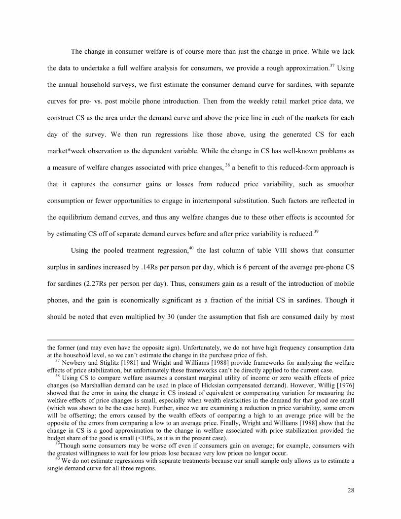
The change in consumer welfare is of course more than just the change in price. While we lack

the data to undertake a full welfare analysis for consumers, we provide a rough approximation.37 Using

the ann

e-phone CS

for sard

should be noted that even multiplied by 30 (under the assumption that fish are consumed daily by most

ual household surveys, we first estimate the consumer demand curve for sardines, with separate

curves for pre- vs. post mobile phone introduction. Then from the weekly retail market price data, we

construct CS as the area under the demand curve and above the price line in each of the markets for each

day of the survey. We then run regressions like those above, using the generated CS for each

market*week observation as the dependent variable. While the change in CS has well-known problems as

a measure of welfare changes associated with price changes, 38 a benefit to this reduced-form approach is

that it captures the consumer gains or losses from reduced price variability, such as smoother

consumption or fewer opportunities to engage in intertemporal substitution. Such factors are reflected in

the equilibrium demand curves, and thus any welfare changes due to these other effects is accounted for

by estimating CS off of separate demand curves before and after price variability is reduced.39

Using the pooled treatment regression,40 the last column of table VIII shows that consumer

surplus in sardines increased by .14Rs per person per day, which is 6 percent of the average pr

ines (2.27Rs per person per day). Thus, consumers gain as a result of the introduction of mobile

phones, and the gain is economically significant as a fraction of the initial CS in sardines. Though it

the former (and may even have the opposite sign). Unfortunately, we do not have high frequency consumption data at the household level, so we can’t estimate the change in the purchase price of fish. 37 Newbery and Stiglitz [1981] and Wright and Williams [1988] provide frameworks for analyzing the welfare effects of price stabilization, but unfortunately these frameworks can’t be directly applied to the current case. 38 Using CS to compare welfare assumes a constant marginal utility of income or zero wealth effects of price changes (so Marshallian demand can be used in place of Hicksian compensated demand). However, Willig [1976] showed that the error in using the change in CS instead of equivalent or compensating variation for measuring the welfare effects of price changes is small, especially when wealth elasticities in the demand for that good are small (which was shown to be the case here). Further, since we are examining a reduction in price variability, some errors will be offsetting; the errors caused by the wealth effects of comparing a high to an average price will be the opposite of the errors from comparing a low to an average price. Finally, Wright and Williams [1988] show that the change in CS is a good approximation to the change in welfare associated with price stabilization provided the budget share of the good is small (<10%, as it is in the present case). 39Though some consumers may be worse off even if consumers gain on average; for example, consumers with the greatest willingness to wait for low prices lose because very low prices no longer occur. 40 We do not estimate regressions with separate treatments because our small sample only allows us to estimate a single demand curve for all three regions.

28

households), when compared to the average monthly expenditure per capita of 678 Rs (estimated from the

household survey), the gain is very small (though if similar gains arise in the market for other commonly

consumed goods, the overall consumer gains relative to expenditure might be larger).

VI. CONCLUSION

We find that the addition of mobile phones reduced price dispersion and waste, and increased

fishermen’s profits and consumer welfare. These results demonstrate the importance of information for

the functioning of markets, and the value arkets; information makes markets work,

and ma

ts in non-

of well-functioning m

rkets improve welfare. And it is again worth emphasizing that the results represent persistent

rather then one-time gains, since market functioning should be permanently enhanced by the availability

of mobile phones. As mentioned earlier, information technologies are often considered a low priority for

developing countries relative to needs in areas such as health and education. However, not only can such

technologies increase earnings, but those increased earnings (or increased purchasing power, due to

reduced consumer prices) in turn can be expected to lead to improvements in health and education. In

addition, because mobile phones in Kerala are a private sector initiative rather than a development

project, other than through perhaps raising interest rates for capital, they do not crowd out investments in

other projects. Also unlike most development projects, the service is self-sustaining; mobile phone

companies provide service because it is profitable to do so, and fishermen are willing to pay for mobile

phones because of the increased profits they receive. This point is also relevant for reconciling our results

with anecdotal evidence that government or NGO projects setting up internet kiosks or other information

services for farmers in other developing countries often do not meet similar success. The welfare gains to

be had are directly tied to, and in fact are indicated by, the profitability of both arbitrage and mobile

phone provision, and the private sector may be better suited to identifying such opportunities.

In generalizing the results, it should be noted that the perishability of fish is an important reason

why there was so much waste and inefficiency before mobile phones and why better information has such

a large impact on market performance and welfare. While there is evidence that even marke

29

perishab

be found

among

le commodities such as grains are often not well-integrated spatially, the biggest gains will likely

be for other perishable commodities, such as milk, eggs, fruits and vegetables, and possibly even day

labor, where spot labor markets often only clear locally (within villages). And there may be other factors

relevant for market performance that interact with the availability of information, such as transportation

infrastructure. For example, more recently in Kerala, improvements in roads have lowered the cost of land

transport, leading to more arbitrage by wholesalers on land (and less by fishermen) since transport is now

in many cases cheaper by road than by sea. In other cases, poor quality roads may limit the ability of

improvements in information to enhance market performance because arbitrage remains prohibitively

expensive. However, the widespread, voluntary adoption of ICTs for marketing by producers and traders

observed in many developing countries suggests similar gains are likely to be found elsewhere.

Finally, in many countries, including India, there is a concern over a perceived internal digital

divide, with both ICT access and the resulting benefits available only to the wealthiest or most educated,

leaving all others behind. However, the evidence here suggests that the benefits of ICTs can

fishermen or farmers, not just software engineers or call-center workers. Further, while it was

primarily the largest fishermen who adopted mobile phones in the present case, there were significant

spillover gains for the smaller fishermen who did not use phones, due to the improved functioning of

markets. Thus, rather than simply excluding the poor or less educated, the ‘digital provide’ appears to be

shared more widely throughout society.

30

APPENDIX. PROOF OF THE THEOREMS

PROOF OF THEOREM 1. Suppose there exists an equilibrium and that p* represents the equilibrium

price difference between the two markets when one catchment zone is in state H and the other is in state

L. Let ( )xπ represent the updated probability that a zone is in state H for a fisherman with catch x. By

switching markets, the fisherman gains *x p with probability ( ) / 2xπ (the probability that their zone is in

state H and the other is in state L) and loses *x p with probability ( )( )1 xπ− / 2 (the probability their zone

is L and the other zone is H); with probability ½, the two zones are in the same state and they receive the

same price as if they did not switch.41 The equilibrium condition for switching is thus ( )( )1/ 2 *x xpπ τ− > .

( )xπ is increasing in x since ( |i i )f x d satisfies the Monotone Likelihood Ratio Property, so the left-hand

side of the previous equation is increasing in x, meaning that only fishermen with the highest values of x

switch markets. Any equilibrium must therefore be based on a cutoff value of x, where all fishermen with

catch greater than this value switch to the other market and all those below sell locally.42 It is then

straightforward to construct the equilibrium by walking down the distribution of catch from xmax to 0 to

identify the cutoff value, ( )x τ . If ( )( )max max1/ 2 *x x pτ π> − , transportation costs are too high (given the

uncertainty over the state of both zones) and no one switches in equilibrium. For smaller values of τ,

some fishermen will switch to the other market. Let ( )*p x represent the level of price dispersion between

the markets when the two zones are in opposite states and fishermen with catch x or above switch

markets. is weakly increasing in the cutoff value x since fewer fishermen are switching as x

increases. The equilibrium cutoff x* for switching is defined implicitly by the equation

( )*p x

( )( ) ( )* 1/ 2 * * *x x p xπ τ− = . Each term on the left-hand side is increasing in x, so x is an increasing

function of τ whenever there is an interior solution to this equation ( max0 *x x< < ). So long as τ is

41 The equilibrium must be symmetric. So when both zones are in the same state, an equal amount of fish flows from each zone to the other, leaving quantities and price equal in the two markets. 42 The equilibrium cannot involve a ‘gap’ in who switches (i.e., a fisherman with x<x(τ)), since if it is worth it for that fisherman to switch, it would also be worth it for all fishermen with catch above them to switch as well.

31

positive, this equation cannot be satisfied near 0x = ; it will never be worthwhile for a fisherman with a

very small catch to switch markets. Thus, for ( )( ) ( ) ( )( )max max1/ 2 L Hx x P Q P Qτ π< − − , there must be an

interior solution x* to the equation above. And since ( )*p x is increasing in x and the equilibrium cutoff x

is increasing in τ, price dispersion as an implicit function of τ, ( )*p τ , must also be increasing in τ.

Finally, consider again the equilibrium condition for switching, ( )( ) ( )* 1/ 2 * *x x p xπ τ− = . The first term

on the left-hand side, , the assessed likelihood that your zone is in an H-state and the other is

in an L-state, reflects uncertainty regarding the state of both one’s own zone and the other zone. Because

this term will always be less than one (even if the state of one’s own zone were known with certainty,

nothing is known about the other zone), equilibrium price dispersion

( )( * 1/ 2xπ − )

( )*p x will always exceed τ/x*, the

per unit transportation costs for the marginal switcher.

PROOF OF THEOREM 2. The proof follows that for Theorem 1 closely. Assuming that τ >τ* allows us

to focus on the case where there is no switching in equilibrium if there is no search technology. We first

show that fishermen with the largest catches gain the most from purchasing the search technology. By

purchasing the search technology, the fisherman gains *x p τ− in revenue with probability ( ) / 2xπ (the

probability that their zone is in state H and the other is in state L). So the equilibrium condition for

purchasing the technology is ( )( )( )/ 2 *x xpπ τ− > Ψ . Since ( )xπ is increasing in x, the left-hand side of

the previous equation is increasing in x, meaning that only fishermen with the highest values of x

purchase the search technology, and any price discovery equilibrium must be based on a cutoff value of x.

We again construct the equilibrium by walking down the distribution of catch from xmax to 0 to identify

the cutoff value, now ( )x Ψ , where all fishermen with catch greater than the threshold buy the search

technology and all those below do not. If ( )( ) ( ) ( )( )( )max max/ 2 L Hx x P Q P Qπ τΨ > − − , information is too

costly and no one purchases the search technology in equilibrium, which reproduces the no-arbitrage case.

32

For smaller values of Ψ, some fishermen will purchase it. The equilibrium cutoff x* for purchasing the

search technology is defined implicitly by ( )( ) ( )( )* / 2 *x xp xπ τ− = Ψ . As above, each term on the left-

hand side is increasing in x so x is an increasing function of Ψ whenever there is an interior solution to

this equation ( max0 *x x< < ). As stated, if ( )( ) ( ) ( )( )( )max max/ 2 L Hx x P Q P Qπ τΨ > − − , there is no interior

solution. So long as τ is positive, this equation cannot be satisfied near 0x = ; it will never be worthwhile

for a fisherman with a very small catch to switch markets, so they will never pay to acquire price

information. Thus, for ( )( ) ( ) ( )( )( )max max/ 2 L Hx x P Q P Qπ τΨ < − − , there must be an interior solution x* to

the equation above. And since is increasing in x and the equilibrium cutoff x is increasing in Ψ,

price dispersion as an implicit function of the cost of search,

( )*p x

( )*p Ψ , must also be increasing in Ψ (and

thus reductions in Ψ weakly reduce ( )*p x ). Finally, note also that from the equilibrium condition for

purchasing the phone, we can see that as Ψ goes to zero, the cutoff for purchase is driven to the x that

would switch if both zones were known with certainty and the zones were in opposite states, and

equilibrium price dispersion p* goes to τ/x.

33

APPENDIX TABLE EFFECTS OF MOBILE PHONE SERVICE ON OUTCOMES AND WELFARE: SEPARATE TREATMENTS

(1) (2) Max-min

spread Coefficient of

variation

(3) % have waste

(4) Quantity

Sold

(5)

Price

(6)

Price (>0)

(7)

Revenue

(8)

Costs

(9)

Profits

Region I -.64 -.01 .005 35 .03 .13 352 -15 367

(.60) (.07) (.005)

(6.8)

(.07)

(.06)

(54)

(9.6)

(49)

Region II -.05 -.07 -.02 32 -.01 -.18 182 .53 182(.60) (.07) (.005)

(6.9)

(.07)

(.06)

(55)

(9.7)

(50)

Period 1 -.98 -.12 -.016 -3.1 .39 .33 85 2.5 83 (.48) (.05) (.004) (5.6)

(.06) (.05) (45) (7.9) (41)

Period 2 -.64 .16 -.021 -14 .54 .44 30 -.91 30(.46) (.05) (.004)

(5.4)

(.05)

(.05)

(43)

(7.5)

(39)

.

Period 3 -5.7 -.55 -.076 18 .85 .29 385 66 319 (.51) (.06) (.004)

(5.9)

(.06)

(.05)

(47)

(8.3)

(43)

-.

RegionI_period1

-4.8 -.42 -.060 25 .16 -.41 199 93 106(.68) (.07) (.005)

(7.7)

(.08)

(.07)

(62)

(11)

(56)

RegionI_period2

-5.6 -.44 -.062 24 .20 -.38 225 81 144(.66) (.07) (.006)

(7.5)

(.07)

(.07)

(60)

(10)

(54)

RegionI_period3

-.73 -.07 -.006 -.36 .07 .15 56 41 15(.72) (.08) (.006)

(8.1)

(.08)

(.07)

(65)

(11)

(59)

RegionII_period1

.09 .05 .004 -9.0 .04 .05 -52 -6.9 -45(.68) (.07) (.005) (7.8)

(.08) (.07) (62) (11) (57)

RegionII_period2

-5.7 -.34 -.036 12 -.01 -.32 197 73 123(.66) (.07) (.005)

(7.6)

(.07)

(.06)

(60)

(10)

(55)

RegionII_period3

-.97 -.01 .018 -9.2 .04 .18 47 22 25(.72) (.08) (.006)

(8.2)

(.09)

(.07)

(65)

(12)

(60)

Observations 747 747 74,700 74,700

74,700

73,335

72,764

74,700

74,700

Data from the Kerala Fisherman Survey conducted by the author. Standard errors, clustered at the village-level, in parentheses. All prices in 2001 Rs.

34

JOHN F. KENNEDY SCHOOL OF GOVERNMENT, HARVARD UNIVERSITY

REFERENCES Alam, Shafiq, “Mobile Rings Changes for World’s Poor,” Sydney Morning Herald, April 22, 2005. Arnold, Wayne, “Cell Phones for the World’s Poor,” The New York Times January 19, 2001: C1. Brown, Jeffrey and Austan Goolsbee, “Does the Internet Make Markets More Competitive? Evidence

from the Life Insurance Industry,” Journal of Political Economy, CX (2002), 481-507. Diamond, Peter. “A Model of Price Adjustment,” Journal of Economic Theory, III (1971), 156-168. England, Andrew. “African Farmers Discover Technology’s Benefits,” Financial Times November 24,

2004, London Edition: Middle East & Africa, 9. Gates, Bill. www.microsoft.com/billgates/speeches/2000/10-18digitaldividends.asp (2000). Giné, Xavier and Stefan Klonner, “Financing a New Technology: The Dynamics of Linked Product and

Credit Contracts in South-Indian Small-Scale Fishery,” mimeo, Cornell University. Government of Kerala, Annual Profile: Draft Fisheries Policy. Thiruvananthapuram, Kerala, 2005. Kurien, John, “Factoring Social and Cultural Dimensions into Food and Livelihood Security Issues of

Marine Fisheries: A Case Study of Kerala State, India,” Centre for Development Studies, Thiruvananthapuram, Working Paper No. 299, 2000.

LaFraniere, Sharon, “Cellphones Catapult Rural Africa to 21st Century,” The New York Times August 25, 2005: A1.

Massell, Benton F., “Price Stabilization and Welfare,” Quarterly Journal of Economics, LXXXIII (1969), 284-298.

Newbery, David M.G. and Joseph E. Stiglitz, The Theory of Commodity Price Stabilization: A Study in the Economics of Risk (Oxford: Clarendon Press 1981).

Oi, Walter Y., “The Desirability of Price Instability Under Perfect Competition,” Econometrica, XXIX (1961), 58-64.

Platteua, Jean-Philippe, “The Drive Towards Mechanization of a Small-Scale Fisheries in Kerala: A Study of the Transformation Process of Traditional Village Societies,” Development and Change 15 (1984), 65-103.

Rai, Saritha , “In Rural India, A Passage To Wirelessness,” The New York Times August 4, 2001: C1. Roller, Lars-Hendrik and Leonard Waverman, “Telecommunications Infrastructure and Economic

Development: A Simultaneous Equations Approach,” American Economic Review, XCI (2001), p. 909-23.

Rothschild, Michael, “Models of Market Organization with Imperfect Information: A Survey,” Journal of Political Economy, LXXXI (1973), 1283-1308.

Stigler, George, “The Economics of Information,” Journal of Political Economy, LXIX (1961), 213-225. Stiglitz, Joseph, “Imperfect Information in the Product Market,” in Schmalensee, Richard and Robert

Willig, eds., Handbook of Industrial Organization, Volume I. (Elsevier Science Publishers B.V.: Amsterdam, 1989), p. 769-847.

Waugh, Frederick V., “Does the Consumer Benefit from Price Instability?” Quarterly Journal of Economics, LVIII (1944), 602-614.

Willig, Robert D., “Consumer’s Surplus Without Apology,” American Economic Review, LVI (1976), 589-97.

Wright, Brian, “Storage and Price Stabilization,” in Gardner, Bruce L. and Gordon C. Rausser, eds., Handbook of Agricultural Economics, Volume 1B. (Elsevier Science Publishers B.V.: Amsterdam, 2001), p. 817-862.

-- and Jeffrey C. Williams, “Measurement of Consumer Gains from Market Stabilization,” American Journal of Agricultural Economics, LXX (1988), 616-27.

35

TABLE I

PRICES AND EXCESS SUPPLY AND DEMAND IN 15 SARDINE BEACH MARKETS

Price (Rs/kg) Excess buyers Excess sellers

Kasaragod District

Hosabethe 6.2 0 0

Aarikkadi 4.0 0 0

Kasaba 0.0 0 4

Kanhangad 7.2 0 0

Thaikadappuram 9.7 11 0

Kannur District

Puthiangadi 8.7 2 0

Neerkkadavu 6.9 0 0

Ayikkara 8.4 1 0

Thalassery 4.3 0 0

New Mahe 6.2 0 0

Kozhikode District

Chombala 9.9 15 0

Badagara 0.0 0 11

Quilandi 9.8 12 0

Puthiyangadi 0.0 0 6

Chaliyam 6.4 0 0

Data from the Kerala Fisherman Survey conducted by the author. The first column contains the average 7:45-8:00AM price of sardines in each market on Tuesday, January 14, 1997, in rupees per kilogram. The markets are listed in north-south geographic alignment; starting from Hosabethe, the distance in kilometers between each market and the next is: 12, 14, 15, 15, 24, 15, 6, 14, 9, 8, 7, 15, 10, and 16. “Excess buyers” represents the number of buyers who leave the market without having purchased enough fish, and “excess sellers” is the number of fishermen who leave the market without selling their fish.

36

TABLE II MOBILE PHONE INTRODUCTION AND CHANGES IN FISH MARKETING BEHAVIOR

Period 0 (pre-phone)

Period 1 (region I

adds phones)

Period 2 (region II

adds phones)

Period 3 (region III

adds phones)

% of fishermen who fish in local catchment zone

Region I .98 .99 .98 .98 (.003) (.001) (.001) (.002)

Region II .99 .98 .99 .99 (.002) (.001) (.01) (.001)

Region III .98 .98 .98 .99 (.002) (.001) (.001) (.001)

% of fishermen who sell in local catchment zone Region I 1.00 .66 .63 .62 (0.00) (.005) (.005) (.006)

Region II 1.00 1.00 .64 .58 (0.00) (0.00) (.004) (.006)

Region III 1.00 1.00 1.00 .70 (0.00) (0.00) (0.00) (.005) Number of fishing units

Region I 83 85 85 89

Region II 69 74 75 75

Region III 53 55 54 56

Data from the Kerala Fisherman Survey conducted by the author, using fishermen’s self-report of fishing location and market of sale. The catchment zone for each town is the area of sea defined by lines extending out to sea at the midpoint between a town and its nearest neighbors to the north and south. Regions and periods are as defined in the text. Standard errors in parentheses.

37

TABLE III PRICE DISPERSION AND WASTE IN KERALA SARDINE MARKETS

Period 0

(pre-phone)

Period 1 (region I

adds phones)

Period 2 (region II

adds phones)

Period 3 (region III

adds phones)

Max-min spread (Rs/kg)

Region I 7.60 1.86 1.32 1.22 (.50) (.22) (.10) (.44)

Region II 8.19 7.30 1.79 1.57 (.44) (.29) (.19) (.16)

Region III 8.24 7.27 7.60 2.56 (.47) (.27) (.25) (.34)

Coefficient of variation (%)

Region I .68 .14 .08 .07 (.07) (.01) (.01) (.01)

Region II .62 .55 .12 .08 (.04) (.04) (.01) (.01)

Region III .69 .57 .54 .14 (.09) (.04) (.03) (.02)

Waste (%)

Region I .08 .00 .00 .00 (.01) (.00) (.00) (.00)

Region II .05 .04 .00 .00 (.01) (.01) (.00) (.00)

Region III .07 .06 .06 .00 (.01) (.01) (.01) (.00)

Data from the Kerala Fisherman Survey conducted by the author. Period and regions are as defined in the text. The max-min spread is the difference between the highest and lowest 7:30-8:00AM average price on a given day among the five markets making up each region, in year 2001 Rs/kg. The coefficient of variation is the standard deviation of the 7:30-8:00AM average price on a given day across the five markets within each region divided by the mean 7:30-8:00AM average price for each region. Waste refers to the percent of fishermen who report not selling their catch. Standard errors in parentheses.

38

TABLE IV EFFECTS OF MOBILE PHONE SERVICE ON PRICE DISPERION AND WASTE:

POOLED TREATMENTS

(1)

Max-min spread

(2) Coefficient of

variation

(3) % have Waste

(4) Max-min

spread

(5) Coefficient of variation

(6) % have waste

Phone -5.0 -.38 -.048 -5.3 -.41 -.047 (.27) (.03) (.004) (2.9) (.32) (.06)

Region I -.92 -.06 -.007 -.94 -.06 -.006 (.26) (.03) (.005) (.26) (.03) (.005)

Region II -.46 -.04 -.011 -.46 -.04 -.011 (.21) (.02) (.004) (.21) (.02) (.005)

Period 1 -.89 -.12 -.017 -.84 -.12 -.016 (.29) (.04) (.008) (.29) (.03) (.008)

Period 2 -1.1 -.17 -.019 -1.0 -.16 -.018 (.32) (.04) (.008) (.33) (.04) (.008)

Period 3 -1.2 -.19 -.022 -1.2 -.19 -.021 (.40) (.04) (.009) (.40) (.04) (.009)

Fuel cost .02 .01 .001 -.13 -.02 .003 (.12) (.01) (.002) (.19) (.02) (.005)

Wind/Sea Index .086 .001 -.002 -.03 -.01 -.003 (.051) (.004) (.002) (.06) (.01) (.003)

Phone*Fuel cost .25 .026 -.003 (.14) (.014) (.006)

Phone*Wind/Sea Index .19 .021 .003 (.08) (.008) (.005)

Number of Observations 747 747 74,700 747 747 74,700

Data from the Kerala Fisherman Survey conducted by the author. The variable Phone is assigned a value of 1 for all dates in which a region has mobile phone service available. All prices are in 2001 Rs. Standard errors, clustered at the village-level for columns (3) and (6), in parentheses.

39

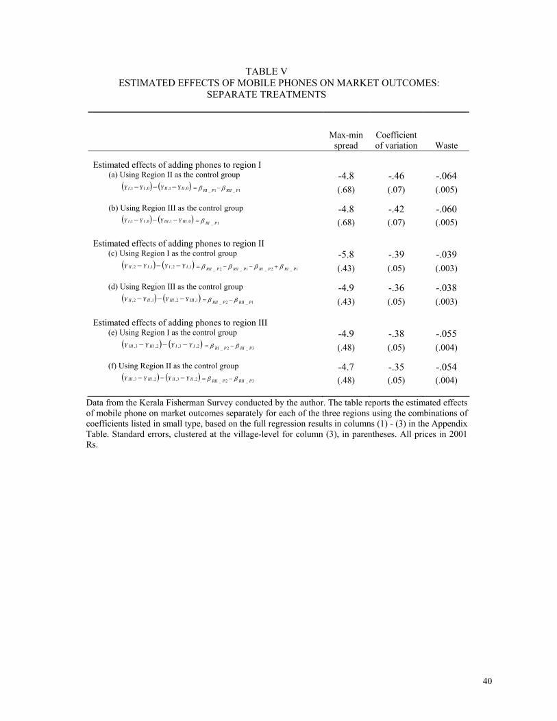
TABLE V ESTIMATED EFFECTS OF MOBILE PHONES ON MARKET OUTCOMES:

SEPARATE TREATMENTS

Max-min

spread Coefficient of variation

Waste

Estimated effects of adding phones to region I (a) Using Region II as the control group -4.8 -.46 -.064

( ) ( ) ββ 1_1_ PRIIPRI −= YYYY IIIIII 0,1,0,1, −−−

YYYY IIIIIIII 0,1,0,1, −−−

YYYY IIIII 1,2,1,2, −−−

YYYY IIIIIIIIII 1,2,1,2, −−−

YYYY IIIIIIII 2,3,2,3, −−−

YYYY IIIIIIIIII 2,3,2,3, −−−

(.68) (.07) (.005) (b) Using Region III as the control group -4.8 -.42 -.060

( ) ( ) β 1_ PRI= (.68) (.07) (.005)

Estimated effects of adding phones to region II (c) Using Region I as the control group -5.8 -.39 -.039

( ) ( ) ββββ 1_2_1_2_ PRIPRIPRIIPRII +−−= (.43) (.05) (.003)

(d) Using Region III as the control group -4.9 -.36 -.038 ( ) ( ) ββ 1_2_ PRIIPRII −= (.43) (.05) (.003)

Estimated effects of adding phones to region III

(e) Using Region I as the control group -4.9 -.38 -.055 ( ) ( ) ββ 3_2_ PRIPRI −= (.48) (.05) (.004)

(f) Using Region II as the control group -4.7 -.35 -.054

( ) ( ) ββ 3_2_ PRIIPRII −= (.48) (.05) (.004)

Data from the Kerala Fisherman Survey conducted by the author. The table reports the estimated effects of mobile phone on market outcomes separately for each of the three regions using the combinations of coefficients listed in small type, based on the full regression results in columns (1) - (3) in the Appendix Table. Standard errors, clustered at the village-level for column (3), in parentheses. All prices in 2001 Rs.

40

TABLE VI TESTING ALTERNATIVE EXPLANATIONS

Supply ‘Maximum Dispersion’ Prices Predicted Prices (1)

Quantity (kg)

(2) Coefficient of Variation

(3) Max-min

spread

(4) Coefficient of variation

(5) Max-min

spread

(6) Coefficient of variation

(7)

Waste

Phone -1.4 -.02 -4.5 -.34 -4.4 -.31 -.048 (9.2) (.04) (.34) (.04) (2.9) (.30) (.06)

Region I 33 -.08 -.77 -.06 -.91 -.06 -.006 (8.0) (.04) (.31) (.04) (.28) (.02) (.005)

Region II 17 -.06 -.48 -.03 -.43 -.06 -.011 (.21) (.03) (.23) (.02) (.23) (.03) (.005)

Period 1 -15 -.002 -.80 -.08 -.79 -.11 -.016 (14) (.04) (.29) (.03) (.24) (.04) (.008)

Period 2 -28 .05 -.98 -.13 -1.1 -.14 -.018 (18) (.05) (.31) (.04) (.31) (.04) (.008)

Period 3 -20 .03 -1.1 -.17 -.98 -.21 -.021 (20) (.06) (.38) (.04) (.39) (.03) (.009)

Number of Observations 74,700 747 747 747 747 747 74,700

Data from the Kerala Fisherman Survey conducted by the author. The variable Phone is assigned a value of 1 for all dates in which a region has mobile phone service available. All prices are in 2001 Rs. Column (1) uses fisherman-level observations on catch for the dependent variable, while column (2) uses the coefficient of variation of estimated total catch across markets within a region. Columns (3) and (4), ‘Maximum Dispersion’ Prices, estimate the pooled treatment regressions using the highest values of the coefficient of variation and max-min spread observed during a given market day. Columns (5)-(7) use prices predicted from pre-phone market demand curves for post-phone periods rather than actual prices. Standard errors, clustered at the village-level for columns (1) and (7), in parentheses.

41

TABLE VII

VIOLATIONS OF THE LAW OF ONE PRICE

Period 0

(pre-phone)

Period 1 (region I has

phones)

Period 2 (region II

has phones)

Period 3 (region III

has phones)

Overall

Region I .54 .03 .04 .03

Region II .57 .55 .06 .05

Region III .60 .58 .58 .08

With time + depreciation

Region I .50 .01 .02 .02

Region II .53 .52 .03 .03

Region III .57 .55 .54 .05

All markets combined

Without time + deprec. .47 .35 .20 .05

With time + deprec. .44 .31 .16 .03

Data from the Kerala Fisherman Survey conducted by the author. In the top two panels, the figures represent the average percent of unique market-pairs among the 5 markets in a given region for which the 7:30-8:00AM average price differences differ by more than the estimated transportation costs between the two markets on a given day. For the bottom panel, the figures are for the unique market pairs among all 15 markets in the sample.

42

TABLE VIII EFFECTS OF MOBILE PHONES ON PRODUCERS AND CONSUMERS: POOLED TREATMENTS

(1)Quantity

Sold

(2)

Price

(3)

Price (if >0)

(4)

Revenue

(5)

Costs

(6)

Profits

(7) Profit Users

(8) Profit

Non-User

(9) Consumer

Price

(10) Consumer

Surplus

Phone

23 -.05 -.44 205 72 133 184 97 -.39 .14(8.4) (.03) (.03) (62) (5.6) (60) (90) (47) (.22) (.04)

Region I 36 .25 -.19 370 3.7 367 458 306 .51 -.11 (6.6) (.03) (.03) (56) (4.9) (54) (77) (44) (30) (.03)

Region II

22 .03 -.07 173 3.3 170 204 130 .38 -.03 (5.2) (.02) (.02) (42) (3.0) (40) (57) (35) (.27) (.02)

Period 1 -5.3 .48 .36 66 7.6 58 63 61 .22 -.16(10) (.03) (.03) (59) (4.2) (58) (94) (43) (.05) (.04)

Period 2 -17 .64 .51 34 2.3 32 -6.3 62 .65 -.30(14) (.04) (.03) (80) (3.7) (80) (122) (57) (.27) (.05)

Period 3 -7.8 1.0 .84 215 16 200 212 189 .81 -.48 (16) (.05) (.04) (99) (6.0) (97) (145) (74) (.35) (.05)

Obs. 74,700 74,700 73,335 74,700 74,700 74,700 41,012 33,688 3,735 3,735The data in columns (1)-(8) are from the Kerala Fisherman Survey conducted by the author. Columns (9) and (10) are from the annual household surveys conducted by the author. Standard errors, clustered at the village-level, in parentheses. All prices in 2001 Rs.

43

TABLE IX

EFFECTS OF MOBILE PHONES ON PRODUCERS AND CONSUMERS: SEPARATE TREATMENTS

(1)Quantity

Sold

(2)

Price

(3)

Price (if>0)

(4)

Revenue

(5)

Costs

(6)

Profits

(7) Consumer

Price

Estimated effects of adding phones to region I (a) Using Region II as the control group

( ) ( )35 .11 -.46 251 100 151 -.43

YYYY IIIIII 0,1,0,1, −−− ββ 1_1_ PRIIPRI −= (7.6) (.08) (.07) (60) (11) (57) (.21)

(b) Using Region III as the control group ( ) ( )

25 .16 -.41 199 93 106 -.41 YYYY IIIIIIII 0,1,0,1, −−− β 1_ PRI= (7.7) (.07) (.06) (62) (11) (56) (.22)

Estimated effects of adding phones to region II (c) Using Region I as the control group

( ) ( )22 -.10 -.40 222 92 130 -.39

YYYY IIIII 1,2,1,2, −−− ββββ 1_2_1_2_ PRIPRIPRIIPRII +−−= (4.8) (.05) (.04) (38) (6.8) (35) (.22)

(d) Using Region III as the control group 21 -.06 -.37 248 79 169 -.38 ( ) ( )YYYY IIIIIIIIII 1,2,1,2, −−− ββ 1_2_ PRIIPRII −= (4.9) (.05) (.05) (40) (6.9) (36) (.22)

Estimated effects of adding phones to region III (e) Using Region I as the control group 24 -.07 -.53 169 40 129 -.38

( ) ( )YYYY IIIIIIII 2,3,2,3, −−− ββ 3_2_ PRIPRI −= (5.4) (.05) (.04) (43) (7.7) (40) (.21)

(f) Using Region II as the control group ( ) ( )

21 -.05 -.50 150 51 99 -.38 YYYY IIIIIIIIII 2,3,2,3, −−− ββ 3_2_ PRIIPRII −= (5.5) (.06) (.05) (44) (7.8) (40) (.20)

The data in columns (1)-(6) are from the Kerala Fisherman Survey conducted by the author. Column (7) is from the annual household surveys conducted by the author. The table reports the estimated effects of mobile phone on market outcomes separately for each of the three regions using the combinations of coefficients listed in small type, based on the full regression results in columns (4) - (9) in the Appendix Table. Standard errors, clustered at the village-level, in parentheses. All prices in 2001 Rs.

44

=

L-ZONE Price

QL QL+X Quantity

H-ZONE Price

Quantity QH-X QH

P(QH)

P(QH-X)

A B

C

D E

F

P(QL+X)

P(QL)

FIGURE I. CHANGES IN WELFARE ASSOCIATED WITH ARBITRAGE

45

May 21, 2000

May 21, 2000

July 6, 1998

Ju

REGION III (Kasaragod)

SPREAD OF MOBILE PH

Kanhangad

Kasaragod

FIGURE II

Thalassery

ly 31, 1998

Jan. 31, 1997

REGION II (Kannur)

REGION I (Kozhikode)

Kozhikode

Kannur City

ONE COVERAGE IN KASARAGOD, KANNUR AND KOZHIKODE DISTRICTS

46

.

0 10 20 30 40 50 60 70 80 90 100 110 120 130 140 150 160 170 180 190 200 210 220 230 240 250 Time

0 10 20 30 40 50 60 70 80 90 100 110 120 130 140 150 160 170 180 190 200 210 220 230 240 250 Time

0 10 20 30 40 50 60 70 80 90 100 110 12

0

I

Survey Week

Survey Week

I

0

% w

ith p

hone

0% w

ith p

hone

%

with

pho

ne

TSu

FIGUR

MOBILE PHONE ADOPData from the Kerala Fisherman Survey cond

Phones AddedGION III

Phones Added

REGION

RE

REGION I

Phones Added

1

1

1

0 130 140 150 160 170 180 190 200 210 220 230 240 250 imervey Week

E III TION BY FISHERMEN ucted by the author.

47

02

46

810

1214

0 10 20 30

Pric

e (R

s./k

g)0

24

68

1012

14

0 10 20 30

Pric

e (R

s./k

g)0

24

68

1012

14

0 10 20 30

Pric

e (R

s./k

g)

I

Data from the Kerala8:00AM beach price

Phones Added

40 50 60 70 80 90 100 110 120 130 140 150 160 170 180 190 200 210 220 230 240 250

Time

40 50 60 70 80 90 100 11

40 50 60 70 80 90 100 11

Survey Week

PRICES AND MOB

Fisherman Survey confor average sardines. A

Phones Added

0 120 130 140 150 160 170 180 190 200 210 220 230 240 250

Time

0 120TiSurv

Survey Week

FILE

ducll pr

Phones AddedION III

REGION

REGION II

REG

130 140 150 160 170 180 190 200 210 220 230 240 250me

ey Week

IGURE IV PHONE SERVICE IN KERALA

ted by the author. The price series represent the average 7:30-ices in 2001 Rs.

48