i  

The Development and Control of a Unicycle Robot

  

by    

Surachat Chantarachit    

A dissertation submitted in partial fulfillment of the requirements for  the degree of doctor of Engineering in  

Mechatronics      

Examination Committee:  Prof. Manukid Parnichkun (Chairperson)     Dr. Mongkol Ekpanyapong     Prof. Pennung Warnitchai    

External Examiner:    Prof. Teresa Zielinska     Vice-Dean, Faculty of Power and Aeronautical       Engineering, Warsaw University of Technology     Poland  

    Nationality:  Thai   Previous Degree:  Master of Engineering in Mechatronics      Asian Institute of Technology      Thailand    Scholarship Donor:  Royal Thai Government - AIT Fellowship      

Asian Institute of Technology School of Engineering and Technology 

Thailand May 2017   

 

ii  

ACKNOWLEDGEMENTS

My significant thank to my thesis advisor, Prof. Manukid Parnichkun. This thesis would not be successful  without his obligingness,  invaluable  suggestion and strong  financial support.  I  also  thank  Dr.  Mongkol  Ekpanyapong  and  Prof.  Pennung  Warnitchai,  who helped and suggested me in variety aspects of my research. And thank for contributing their valuable time.  Without  any  help  of  Mechatronic’s  friends,  this  research  could  not  be  completed.  I would  like  to  thank  my  senior;  Dr.  Kanjanapan  Sukvichai,  Mr. Somphop Limsoonthrakul, Mr. Wiput Tuvayanond and also Mr. Choopong Chauypen for sharing their knowledge and providing comments when I got any troubles.  Moreover, I would like to thank secretary staffs; Ms. Chaowaret Sudsaweang and Ms. Pornpun Pugsawade in ISE building.   Last  but  not  least,  I  would  like  to  thank  my  families  and  Ms.  Kanokwan  Singha  for encouraging when I disheartened.   Finally, I would like to thank myself for patience and endeavor to solve the problems in my research.    

 

iii  

ABSTRACT  

Balancing  of  unicycle  robot  is  a  challenging  topic  for  control  and  mechanical  design. The robot has to robustly balance itself in both longitudinal and lateral directions under uncertain  disturbances  and  inherent  non-linear  effects.  This  research  presents  the development and control of a unicycle  robot which utilizes double-flywheel  technique for  roll  (lateral)  control  and  the  inverted-pendulum  technique  for  pitch  (longitudinal) control.  The  non-linear  dynamic  model  is  derived  by  Lagrangian  approach.  The linearized  model  is  approximated  around  upright  position  and  analyzed. The  unicycle robot  prototype  is  designed,  built  and  controlled.  Linear  quadratic  regulator  with integral  action  (LQR+I)  is  proposed  to  balance  the  robot  in  both  directions  and compared with the conventional LQR. Simulation and experimental results of balancing control and robot position control are presented. The results significantly show superior performance of LQR+I over LQR.  Keywords: Unicycle robot, Gyroscopic effect, Non-linear system, Linear quadratic regulator with integral action    

 

iv  

TABLE OF CONTENTS  CHAPTER TITLE PAGE        TITLE PAGE i 

  ACKNOWLEDGEMENTS ii 

  ABSTRACT iii 

  TABLE OF CONTENTS iv 

  LIST OF FIGURES vi 

  LIST OF TABLES viii   LIST OF NOTATIONS ix 

1 INTRODUCTION  1

1.1 Background  1

1.2 Statement of the problem  3

1.3 Objective  4

1.4 Scopes and limitations  4

2 LITERATURE REVIEW  5

2.1 Overview  5

2.2 Robot hardware  6

2.3 Dynamics model  12

2.4 Control algorithm  13

3 UNICYCLE ROBOT HARDWARE  17

3.1 Conceptual design  17

3.2 Mechanical design  22

3.3 Electrical design  24

3.4 Programing  26

4 DYNAMIC MODEL  27

4.1 Robot wheel  27

4.2 Robot frame  28

4.3 Lagrangian and lagrange equation  31

4.4 Model of direct-current (DC) motor  34

4.5 Dynamic model linearization  37

4.6 Robot parameters  50

 

 

v  

5 ROBOT SIMULATION  53

5.1 Linear quadratic regulator  53

5.2 Linear quadratic regulator with integral action  58

6 EXPERIMENTS  63

6.1 Experimental results of robot balancing on flat surface  63

6.2 Experimental results of robot balancing on rough surface  72

7 CONCLUSION AND FUTURE WORK  75

7.1 Conclusion  75

7.2 Future work  75

  REFERENCES  76

  APPENDIX  78

Comments and responses to the paper entitled  78 

Non-linear dynamic model by S-function                 83       

   

 

vi  

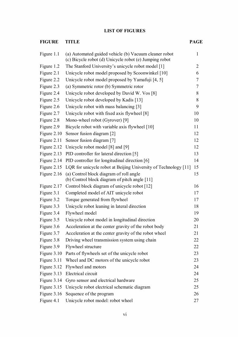
LIST OF FIGURES  

FIGURE TITLE PAGE

Figure 1.1     (a) Automated guided vehicle (b) Vacuum cleaner robot   1                      (c) Bicycle robot (d) Unicycle robot (e) Jumping robot 

Figure 1.2     The Stanford University’s unicycle robot model [1]  2 

Figure 2.1     Unicycle robot model proposed by Scoonwinkel [10]  6 

Figure 2.2     Unicycle robot model proposed by Yamafuji [4, 5]  7 

Figure 2.3     (a) Symmetric rotor (b) Symmetric rotor  7 

Figure 2.4     Unicycle robot developed by David W. Vos [8]  8 

Figure 2.5     Unicycle robot developed by Kadis [13]  8 

Figure 2.6     Unicycle robot with mass balancing [3]  9 

Figure 2.7     Unicycle robot with fixed axis flywheel [8]  10 

Figure 2.8     Mono-wheel robot (Gyrover) [9]  10 

Figure 2.9     Bicycle robot with variable axis flywheel [10]  11 

Figure 2.10   Sensor fusion diagram [2]  12 

Figure 2.11   Sensor fusion diagram [7]  12 

Figure 2.12   Unicycle robot model [8] and [9]  12 

Figure 2.13   PID controller for lateral direction [5]  13 

Figure 2.14   PID controller for longitudinal direction [6]  14 

Figure 2.15   LQR for unicycle robot at Beijing University of Technology [11]  15 

Figure 2.16   (a) Control block diagram of roll angle   15                       (b) Control block diagram of pitch angle [11] 

Figure 2.17   Control block diagram of unicycle robot [12]  16 

Figure 3.1     Completed model of AIT unicycle robot  17 

Figure 3.2     Torque generated from flywheel  17 

Figure 3.3     Unicycle robot leaning in lateral direction  18 

Figure 3.4     Flywheel model  19 

Figure 3.5     Unicycle robot model in longitudinal direction  20 

Figure 3.6     Acceleration at the center gravity of the robot body  21 

Figure 3.7     Acceleration at the center gravity of the robot wheel  21 

Figure 3.8     Driving wheel transmission system using chain  22 

Figure 3.9     Flywheel structure  22 

Figure 3.10   Parts of flywheels set of the unicycle robot  23 

Figure 3.11   Wheel and DC motors of the unicycle robot  23 

Figure 3.12   Flywheel and motors  24 

Figure 3.13   Electrical circuit  24 

Figure 3.14   Gyro sensor and electrical hardware  25 

Figure 3.15   Unicycle robot electrical schematic diagram  25 

Figure 3.16   Sequence of the program  26 

Figure 4.1     Unicycle robot model: robot wheel  27 

 

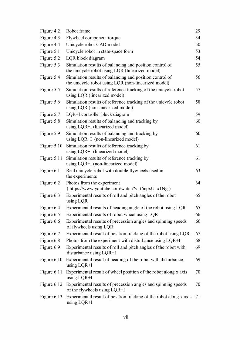
vii  

Figure 4.2     Robot frame  29 

Figure 4.3     Flywheel component torque  34 

Figure 4.4     Unicycle robot CAD model  50 

Figure 5.1     Unicycle robot in state-space form  53 

Figure 5.2     LQR block diagram  54 

Figure 5.3     Simulation results of balancing and position control of    55                      the unicycle robot using LQR (linearized model) 

Figure 5.4     Simulation results of balancing and position control of   56                       the unicycle robot using LQR (non-linearized model) 

Figure 5.5     Simulation results of reference tracking of the unicycle robot    57                      using LQR (linearized model) 

Figure 5.6     Simulation results of reference tracking of the unicycle robot    58                      using LQR (non-linearized model)   

Figure 5.7     LQR+I controller block diagram  59 

Figure 5.8     Simulation results of balancing and tracking by   60                      using LQR+I (linearized model) 

Figure 5.9     Simulation results of balancing and tracking by   60                      using LQR+I  (non-linearized model) 

Figure 5.10   Simulation results of reference tracking by   61                      using LQR+I (linearized model) 

Figure 5.11   Simulation results of reference tracking by   61                      using LQR+I (non-linearized model) 

Figure 6.1     Real unicycle robot with double flywheels used in   63                      the experiments 

Figure 6.2     Photos from the experiment  64                       ( https://www.youtube.com/watch?v=t6npxU_x1Ng ) 

Figure 6.3     Experimental results of roll and pitch angles of the robot   65                      using LQR 

Figure 6.4     Experimental results of heading angle of the robot using LQR  65 

Figure 6.5     Experimental results of robot wheel using LQR  66 

Figure 6.6     Experimental results of precession angles and spinning speeds   66                       of flywheels using LQR 

Figure 6.7     Experimental result of position tracking of the robot using LQR  67 

Figure 6.8     Photos from the experiment with disturbance using LQR+I  68 

Figure 6.9     Experimental results of roll and pitch angles of the robot with    69                       disturbance using LQR+I 

Figure 6.10   Experimental result of heading of the robot with disturbance   69                      using LQR+I 

Figure 6.11   Experimental result of wheel position of the robot along x axis    70                      using LQR+I 

Figure 6.12   Experimental results of precession angles and spinning speeds   70                       of the flywheels using LQR+I 

Figure 6.13   Experimental result of position tracking of the robot along x axis   71                       using LQR+I 

 

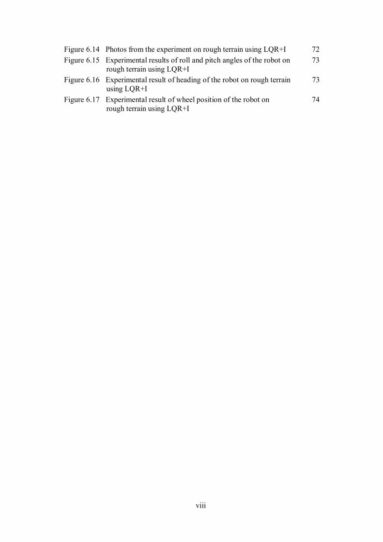
viii  

Figure 6.14   Photos from the experiment on rough terrain using LQR+I  72 

Figure 6.15   Experimental results of roll and pitch angles of the robot on    73                      rough terrain using LQR+I 

Figure 6.16   Experimental result of heading of the robot on rough terrain    73                      using LQR+I 

Figure 6.17   Experimental result of wheel position of the robot on   74                      rough terrain using LQR+I 

   

 

ix  

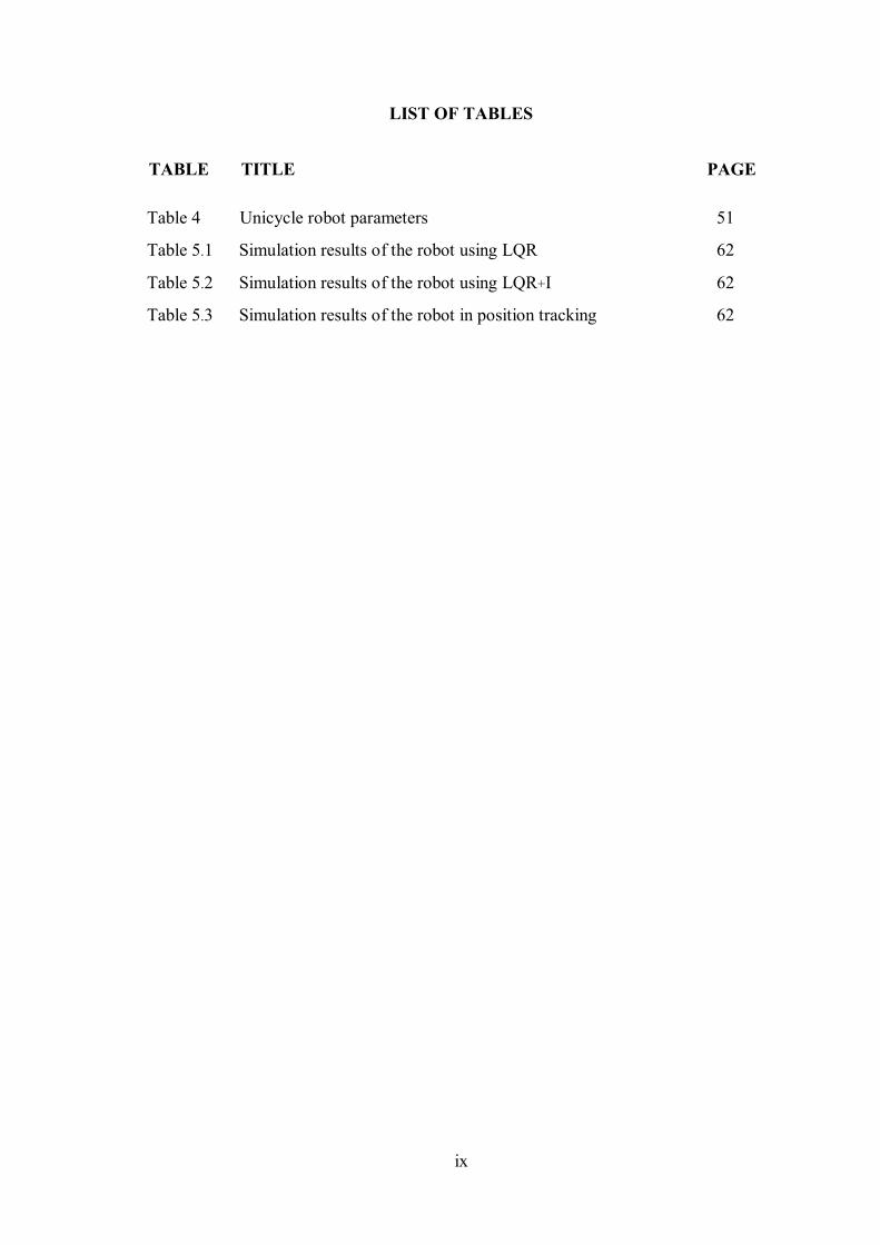
LIST OF TABLES

  TABLE TITLE PAGE

Table 4.        Unicycle robot parameters  51

Table 5.1      Simulation results of the robot using LQR  62

Table 5.2      Simulation results of the robot using LQR+I  62

Table 5.3      Simulation results of the robot in position tracking  62

 

   

 

x  

LIST OF NOTATIONS

The following symbols are used in this report.

A   System matrix 

Ta   Tangent acceleration 

Ra   Radial acceleration 

B   Input matrix C   Coriolis matrix D   Disturbance force F   Generalized actuating force matrix f   Generalized actuating force 

G   Gravity matrix 

rG   Gear transmission ratio 

FI   Moment inertia of the body 

wI   Moment inertia of the wheel 

cFWI   Moment inertia of flywheel 

sJ   Moment of inertia of shaft with flywheel set

J   LQR cost function K   LQR controller gain 

iK   LQR+I controller gain 

tK   Torque constant of the DC motor 

eK   Back-emf (back-electromotive-force) constant 

L Lagrangian is the difference between kinematic energy and potential energy

sL   Angular momentum of the flywheel 

l   Height of the center of gravity 

Fl   Length from robot frame to wheel hub of the unicycle robot  

M   Inertia/mass matrix m   Unicycle robot mass 

wm   Robot wheel mass 

Fm   Robot frame mass 

Q   State weighting matrix 

R   Control weighting matrix R   Armature coil resistance 

0r   Distance from origin point coordinate points to the center of the robot wheel 

1r   Distance from origin point coordinate points to the center of the robot frame 

T   Kinematic energy u   Input vector V   Potential energy 

,V V

  Input voltage 

x   State vector 

0x   exogenous vector with the dynamics 

ex   Error state 

 

xi  

rx   The reference input 

ez   Integral of error ( edt ) 

w   Rotational velocity of the center of mass of the robot wheel 

s    Spinning speed of the flywheel 

, ,,

  Torque input around roll, pitch, yaw and wheel axis 

  Angular precession speed. , , ,   Roll, Pitch, Yaw and Wheel angle 

F   Falling angular acceleration 

( )falling Roll    Falling torque in roll axis 

( )falling Pitch   Falling torque in pitch axis 

 

 

 

1  

CHAPTER 1 INTRODUCTION

1.1 Background

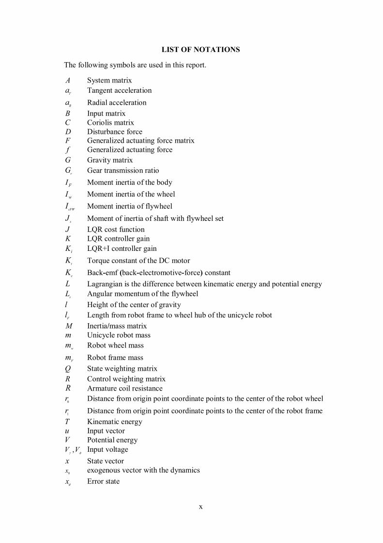
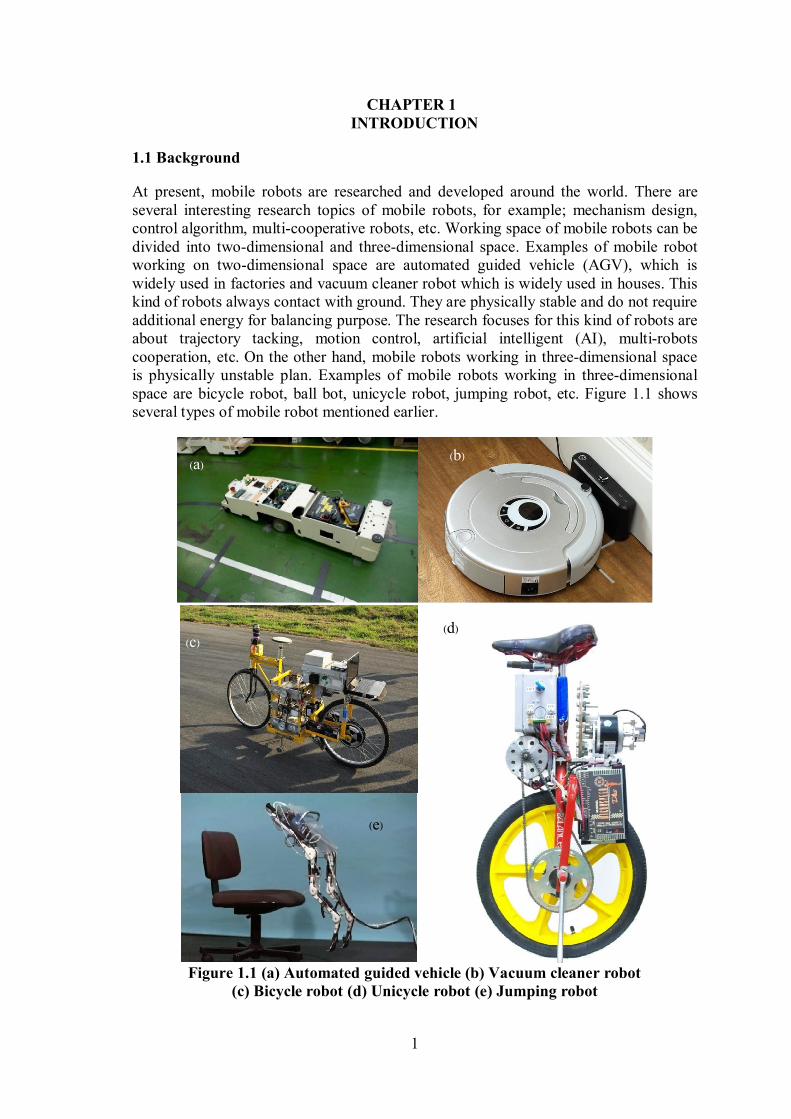
At  present,  mobile  robots  are  researched  and  developed  around  the  world.  There  are several  interesting  research  topics  of  mobile  robots,  for  example;  mechanism  design, control algorithm, multi-cooperative robots, etc. Working space of mobile robots can be divided  into  two-dimensional  and  three-dimensional  space. Examples  of  mobile  robot working  on  two-dimensional  space  are  automated  guided  vehicle  (AGV),  which  is widely used in factories and vacuum cleaner robot which is widely used in houses. This kind of robots always contact with ground. They are physically stable and do not require additional energy for balancing purpose. The research focuses for this kind of robots are about  trajectory  tacking,  motion  control,  artificial  intelligent  (AI),  multi-robots cooperation, etc. On the other hand, mobile robots working  in three-dimensional space is  physically  unstable  plan.  Examples  of  mobile  robots  working  in  three-dimensional space are bicycle  robot, ball  bot, unicycle  robot,  jumping  robot,  etc. Figure 1.1  shows several types of mobile robot mentioned earlier. 

  

Figure 1.1 (a) Automated guided vehicle (b) Vacuum cleaner robot

(c) Bicycle robot (d) Unicycle robot (e) Jumping robot

(d) 

(b) (a) 

(c) 

(e) 

 

2  

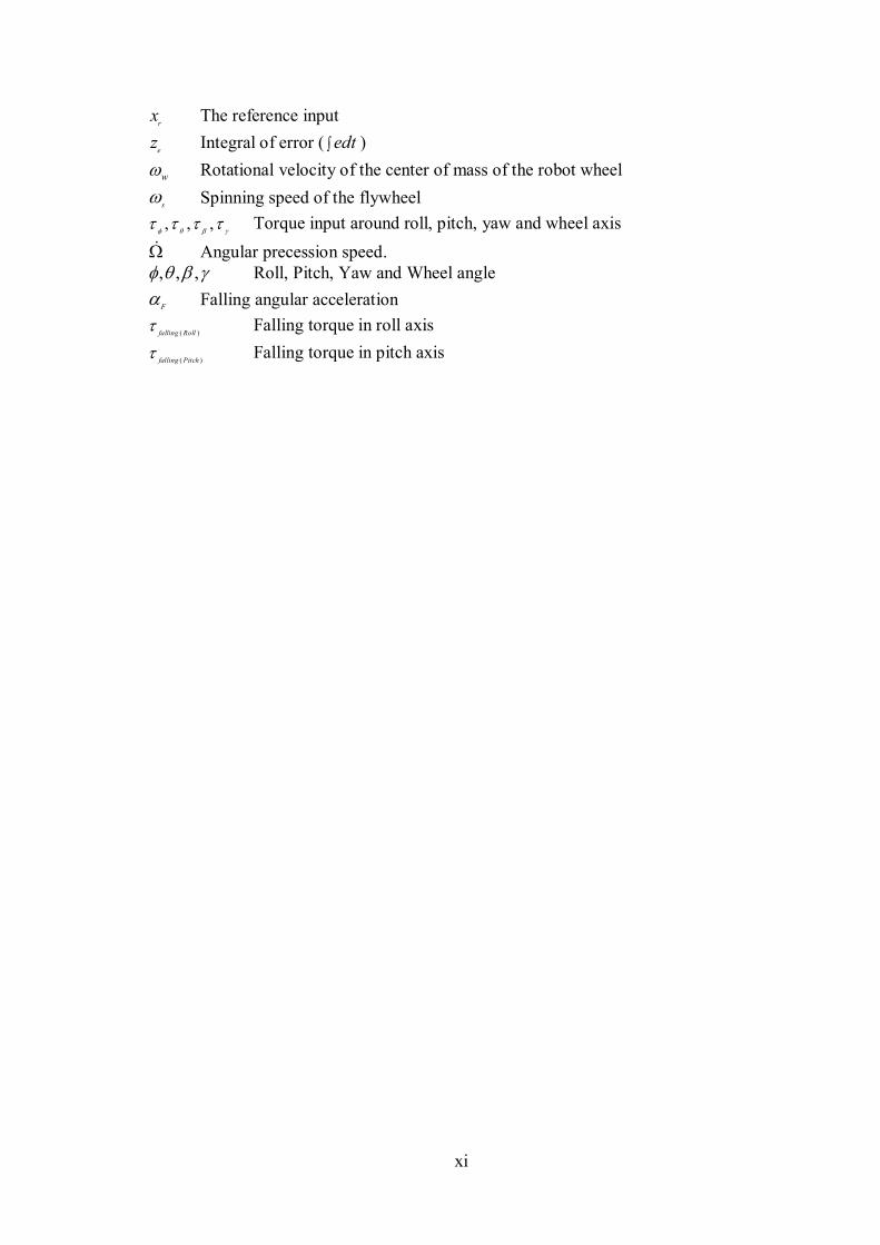
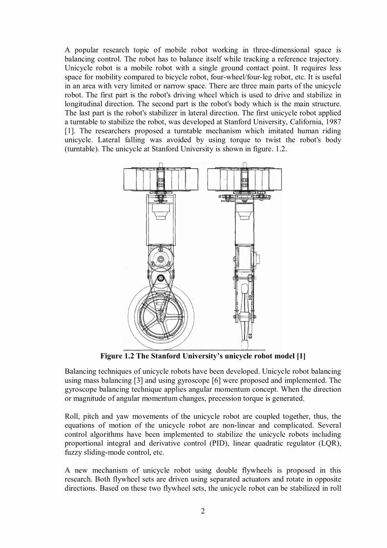
A  popular  research  topic  of  mobile  robot  working  in  three-dimensional  space  is balancing control. The robot has to balance  itself while  tracking a reference trajectory. Unicycle  robot  is  a  mobile  robot  with  a  single  ground  contact  point.  It  requires  less space for mobility compared to bicycle robot, four-wheel/four-leg robot, etc. It is useful in an area with very limited or narrow space. There are three main parts of the unicycle robot. The  first part  is the robot's driving wheel which  is used to drive and stabilize  in longitudinal direction. The second part  is the robot's body which  is the main structure. The last part is the robot's stabilizer in lateral direction. The first unicycle robot applied a turntable to stabilize the robot, was developed at Stanford University, California, 1987 [1].  The  researchers  proposed  a  turntable  mechanism  which  imitated  human  riding unicycle.  Lateral  falling  was  avoided  by  using  torque  to  twist  the  robot's  body (turntable). The unicycle at Stanford University is shown in figure. 1.2.  

 Figure 1.2 The Stanford University’s unicycle robot model [1]

Balancing techniques of unicycle robots have been developed. Unicycle robot balancing using mass balancing [3] and using gyroscope [6] were proposed and implemented. The gyroscope balancing technique applies angular momentum concept. When the direction or magnitude of angular momentum changes, precession torque is generated.   Roll,  pitch  and  yaw  movements  of  the  unicycle  robot  are  coupled  together,  thus,  the equations  of  motion  of  the  unicycle  robot  are  non-linear  and  complicated.  Several control  algorithms  have  been  implemented  to  stabilize  the  unicycle  robots  including proportional  integral  and  derivative  control  (PID),  linear  quadratic  regulator  (LQR), fuzzy sliding-mode control, etc.   A  new  mechanism  of  unicycle  robot  using  double  flywheels  is  proposed  in  this research. Both flywheel sets are driven using separated actuators and rotate in opposite directions. Based on these two flywheel sets, the unicycle robot can be stabilized in roll 

 

3  

and  yaw  axis  at  the  same  time.  As  the  result,  the  rolling  and  heading  angles  of  the unicycle  robot  can  be  controlled  independently. Using  double  flywheel  sets  results  in more torque for roll balancing than using only one flywheel set with the same flywheel size  and  rotating  speed.  In  this  research,  a  unicycle  robot  with  double  flywheels  is introduced.  The  robot's  mechanism  and  electrical  circuit  are  designed  and  developed. The robot is controlled using an optimal controller.  

1.2 Statement of the problem

Balancing  of  unicycle  robot  is  a  very  challenging  and  interesting  topic  for  the researchers  in  dynamic  control  field  because  the  robot  is  a  highly  non-linear  and unstable system. Many unicycle robots have been developed around the world. A well-known balancing technique is the technique of angular momentum (Gyroscope) control. In this dissertation, a unicycle robot with double flywheels is introduced.  Many balancing mechanisms can be applied to balance the unicycle robot. The turntable stabilizer  was  developed  in  [1,  2].  Mass  balancing  technique  was  applied  in  [3,  4]. Balancing  using  angular  momentum  was  applied  in  many  platforms  such  as  mono wheel  robot  [9],  bicycle  robot  [10]  and  also  humanoid  robot.  Double  flywheels  are proposed  to  balance  a  unicycle  in  this  research.  The  advantage  of  balancing  using double flywheels is the high balancing torque. There are also some disadvantage such as many actuators are required and cross coupling between roll and yaw (heading) during balancing.   Balancing  of  the  unicycle  robot  with  double  flywheels  is  complicated  because  it requires  proper  synchronization  of  both  flywheels.  The  flywheels  are  firstly  spun  at constant speeds along vertical axis in order to generate the required angular momentum. Change of the direction of the angular momentum axis by rotating the flywheel axis on front-back  plane  creates  the  rolling  torque.  The  synchronization  of  both  flywheels  is important since it affects the amount of the torque in both roll and yaw directions. Both flywheels are separately controlled and located at the left and the right of the unicycle robot  body. To  simplify  the  dynamic  model,  the  unicycle  robot  model  was  separately considered  in  two  motion  planes  as  applied  in  [3,  4,  5,  6  and  7].  By  the  separated consideration,  the  robot  dynamics  was  decoupled.  In  order  to  determine  relation between the roll and yaw axis, the unicycle robot dynamic model is derived in 3-D and referred to the fixed world coordinate.   The  unicycle  robot  is  required  to  stabilize  at  the  upright  position  and  simultaneously track  the  way  points.  In  this  research,  a  unicycle  robot  with  double  flywheels  is designed, developed and controlled. Linear Quadratic Regulator is proposed to balance the robot.    

 

4  

1.3 Objective

The main objectives of this research are to design a new mechanism to balance unicycle robot and to propose and design a control algorithm to control the unicycle robot.  The objectives can be summarized as  

To design and build a unicycle robot with double flywheels.  To obtain the dynamic model of the unicycle robot.  To propose an optimal control algorithm to balance the unicycle robot at upright 

position and to control trajectory tracking of the robot. 

1.4 Scopes and limitations

The maximum weight of the unicycle robot is 40 kg.  The maximum payload is 60 kg.  The maximum initial leaning angle in each axis is 5 degrees.  The maximum speed of the robot along longitudinal direction is 0.1 m/s.  The friction force is small and neglected.  The ground field is flat and hard. 

 

 

5  

CHAPTER 2 LITERATURE REVIEW

2.1 Overview

Unicycle robot is a mobile robot with a single ground contact. It requires less space for mobility compared to bicycle robot, four-wheel/four-leg robot, etc. It can be useful in an area with very limited or narrow space. Balancing of this kind of robot has been a very challenging  and  interesting  topic  for  the  researchers  in  dynamic  control  because  of  a highly non-linear and unstable system of the robot. It importantly requires the controller that  robustly  stabilizes  the  robot at  the upright position and  simultaneously  tracks  the referenced  command.  The  first  unicycle  robot  was  developed  at  Stanford  University, California, 1987 by A. Schoowinkel  [1] which applied turntable mechanism to imitate human  riding  unicycle.  The  lateral  falling  down  of  robot  was  avoided  by  the  torque from  twisting  the  robot  body.  However,  it  was  unsuccessful  because  of  insufficient torque  generated  by  the  mechanism.  Eight  years  later,  Z. Sheng  and  K.  Yamafuji  [2] improved  the  technique  by  using  an  asymmetric  turntable  that  could  produce  greater torque.  The  simulation  and  experimental  results  showed  that  the  improved  unicycle robot could be balanced. It  is the first success of imitating human riding unicycle. The other techniques is mass balancing, this techniques is based on changing center of mass of the robot by moving a pendulum mass. R. Nakajima et al. from Tsukuba University [3]  proposed  mass  balancing  technique  for  their  rugby  ball-shaped  robot.  They  could balance  the  robot  in  roll  axis  and  could  control  the  robot  steering. Y. Daud  et  al.  [4] proposed  an  approach  of  swinging  a  pendulum  sideward  to  balance  the  robot  in  roll axis.  The  relationship  between  leaning  angle  of  the  robot  and  pendulum  angle  was determined  and  simulated.  J.  H.  Lee  et  al.  from  Chungnam  National  University  [5] introduced a couple of air blowers on opposite sides of their robot in order to produce balancing  force  along  roll  axis.  One  of  the  most  well-known  balancing  technique  is based on angular momentum concept. A spinning wheel, or flywheel, is attached to the robot for maintaining angular momentum. The flywheel is accelerated or decelerated to generate balancing torque in roll axis. S. Majima et al. [6, 7] proposed a single-flywheel technique  for  balancing  a  unicycle  robot.  Daoxiong  G.  et  al.  [8]  applied  a  single flywheel  for  stabilizing  roll  angle  of  the  robot  on  an  inclined  plane.  However,  this technique  is  limited  by  the  maximum  speed  and  acceleration  limit  of  the  motor. Variable  axis  flywheel  is  another  technique  for  balancing  the  robot.  The  flywheel constantly  spins  and  maintains  the  angular  momentum.  When  angular  momentum  is changed by rotating the flywheel axis, it thus produces the rolling torque to the robot. Y. Xu and S. K. W. Au [9] applied this technique for roll-angle balancing of a mono-wheel robot (Gyrover). Their stabilization mechanism is  inside the wheel. Also, B. T. Thanh, and M. Parnichkun [10] utilized the same technique in bicycle robot, called BicyRobo. However,  there  exists  an  inherited  drawback  in  the  form  of  coupled  rolling-heading effect. 

The  unicycle  robot  with  double  flywheels  is  a  system  which  composes  of  two flywheels. The double  flywheels concept  is proposed to decouple roll  and yaw motion which solves the problem occurs in a single flywheel system. As the result, roll and yaw of  the  robot  can  be  controlled  independently.  Furthermore,  the  double  flywheels  can gain more rolling torque than a single flywheel. 

 

6  

2.2 Robot hardware

The  unicycle  robot  is  an  unstable  system.  It  can  fall  in  two  directions;  roll  and  pitch directions. Therefore,  stabilizer  is  an  important  part of  the  hardware.  To  maintain  the robot  in  upright  position,  there  are  several  techniques.  In  this  section,  balancing mechanisms, motors and sensors for the unicycle robot are explained. 

2.2.1 Roll balancing mechanism

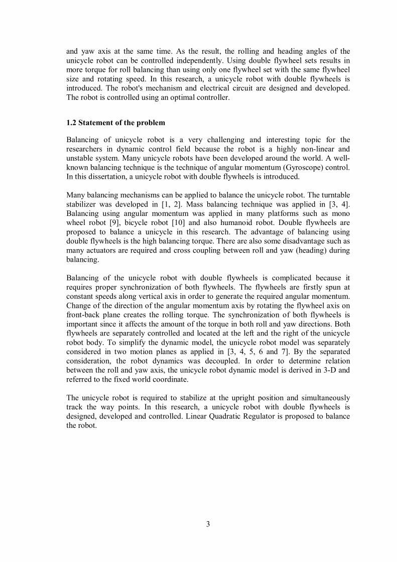
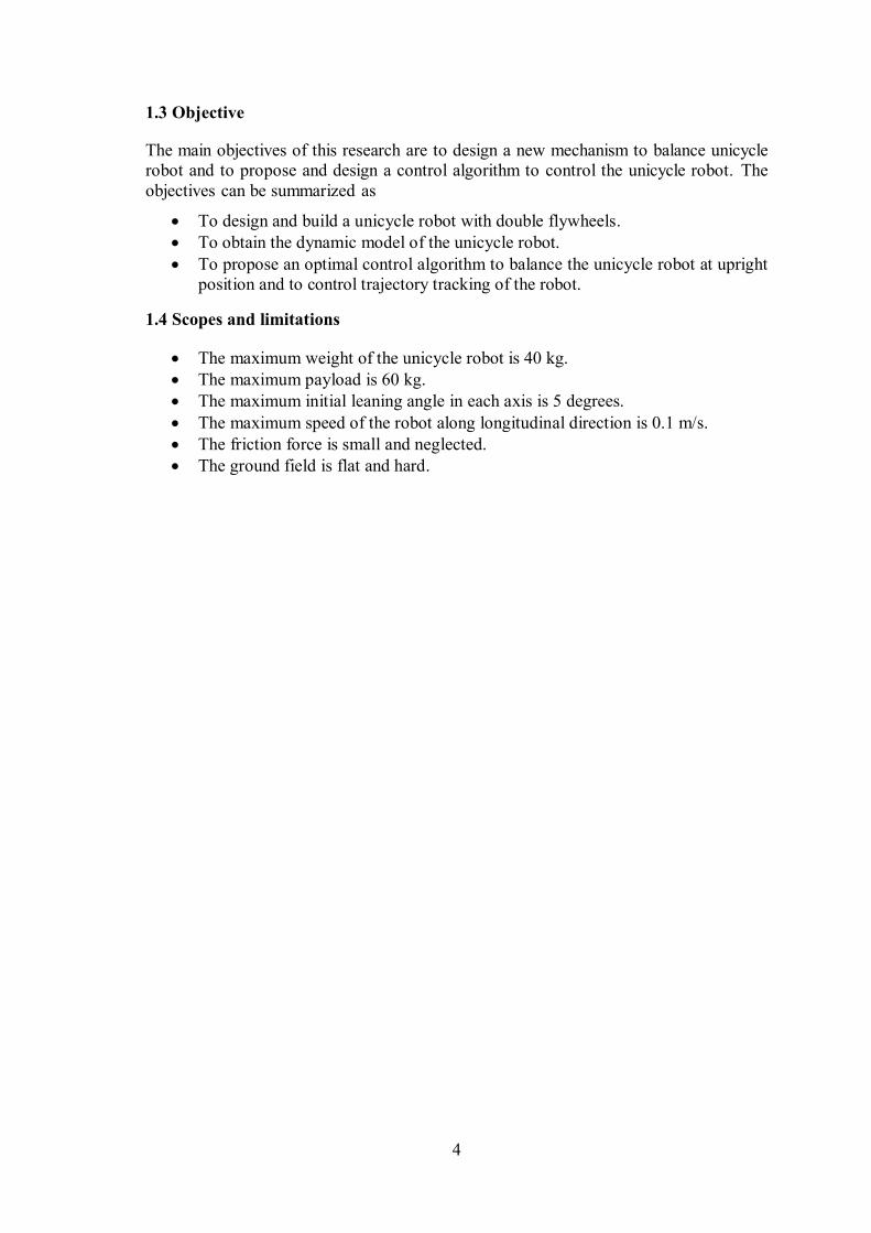
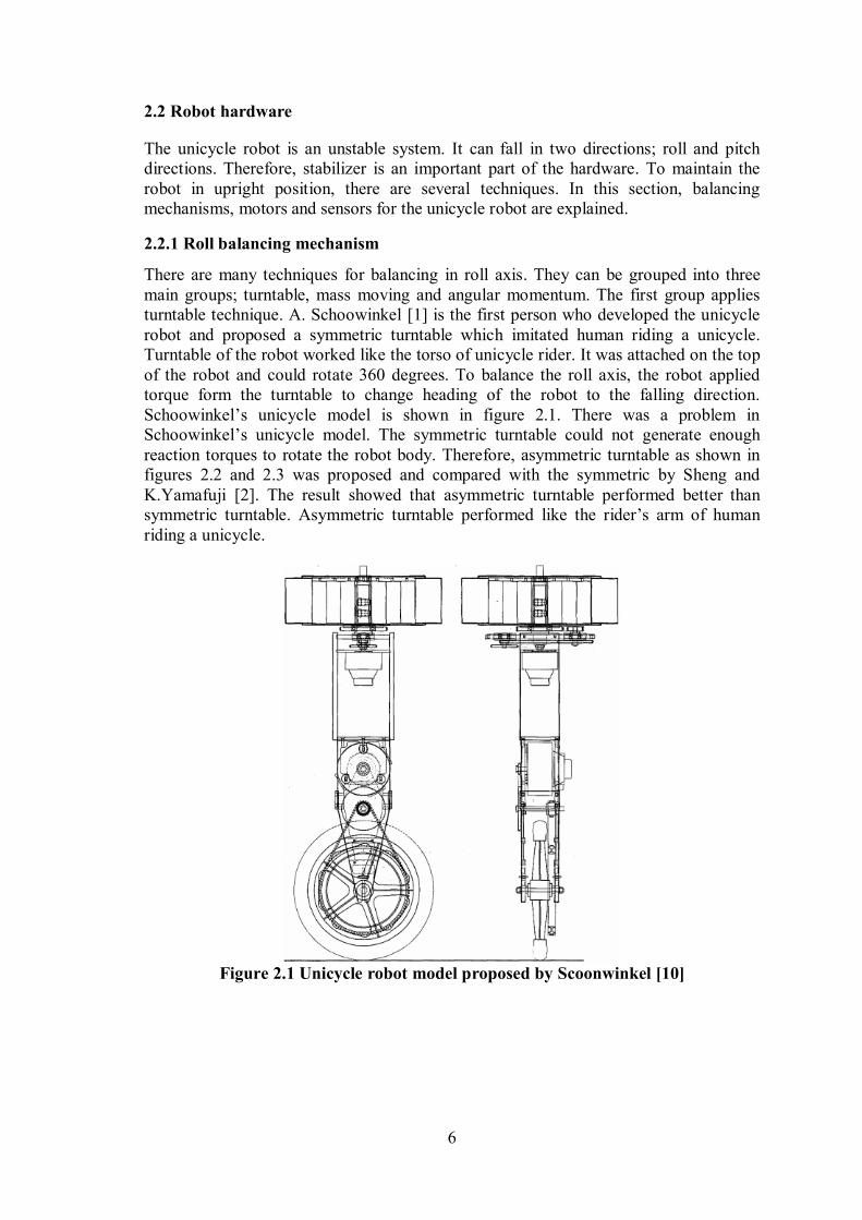
There  are  many  techniques  for  balancing  in  roll  axis. They  can  be  grouped  into  three main  groups;  turntable,  mass  moving  and  angular  momentum. The  first  group  applies turntable technique. A. Schoowinkel [1] is the first person who developed the unicycle robot  and  proposed  a  symmetric  turntable  which  imitated  human  riding  a  unicycle. Turntable of the robot worked like the torso of unicycle rider. It was attached on the top of  the  robot  and  could  rotate  360  degrees. To  balance  the  roll  axis,  the  robot  applied torque  form  the  turntable  to  change  heading  of  the  robot  to  the  falling  direction. Schoowinkel’s  unicycle  model  is  shown  in  figure  2.1.  There  was  a  problem  in Schoowinkel’s  unicycle  model.  The  symmetric  turntable  could  not  generate  enough reaction torques to rotate the robot body. Therefore, asymmetric turntable as shown  in figures  2.2  and  2.3  was  proposed  and  compared  with  the  symmetric  by  Sheng  and K.Yamafuji  [2].  The  result  showed  that  asymmetric  turntable  performed  better  than symmetric  turntable.  Asymmetric  turntable  performed  like  the  rider’s  arm  of  human riding a unicycle.  

 Figure 2.1 Unicycle robot model proposed by Scoonwinkel [10]

 

 

7  

  

 Figure 2.2 Unicycle robot model proposed by Yamafuji [4, 5]

 Figure 2.3 (a) Symmetric rotor (b) Symmetric rotor

   

 

 

8  

 Figure 2.4 Unicycle robot developed by David W. Vos [8] 

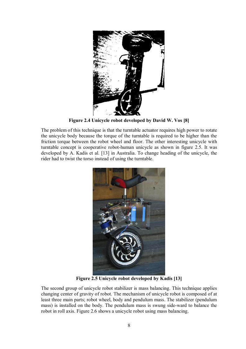
The problem of this technique is that the turntable actuator requires high power to rotate the unicycle body because the torque of  the turntable  is required to be higher  than the friction  torque between  the  robot wheel and  floor. The other  interesting unicycle with turntable  concept  is  cooperative  robot-human  unicycle  as  shown  in  figure  2.5.  It  was developed by A. Kadis et al. [13]  in Australia. To change heading of  the unicycle,  the rider had to twist the torso instead of using the turntable. 

 Figure 2.5 Unicycle robot developed by Kadis [13] 

The second group of unicycle robot stabilizer is mass balancing. This technique applies changing center of gravity of robot. The mechanism of unicycle robot is composed of at least three main parts; robot wheel, body and pendulum mass. The stabilizer (pendulum mass)  is  installed on the body. The pendulum mass  is swung side-ward to balance the robot in roll axis. Figure 2.6 shows a unicycle robot using mass balancing. 

 

9  

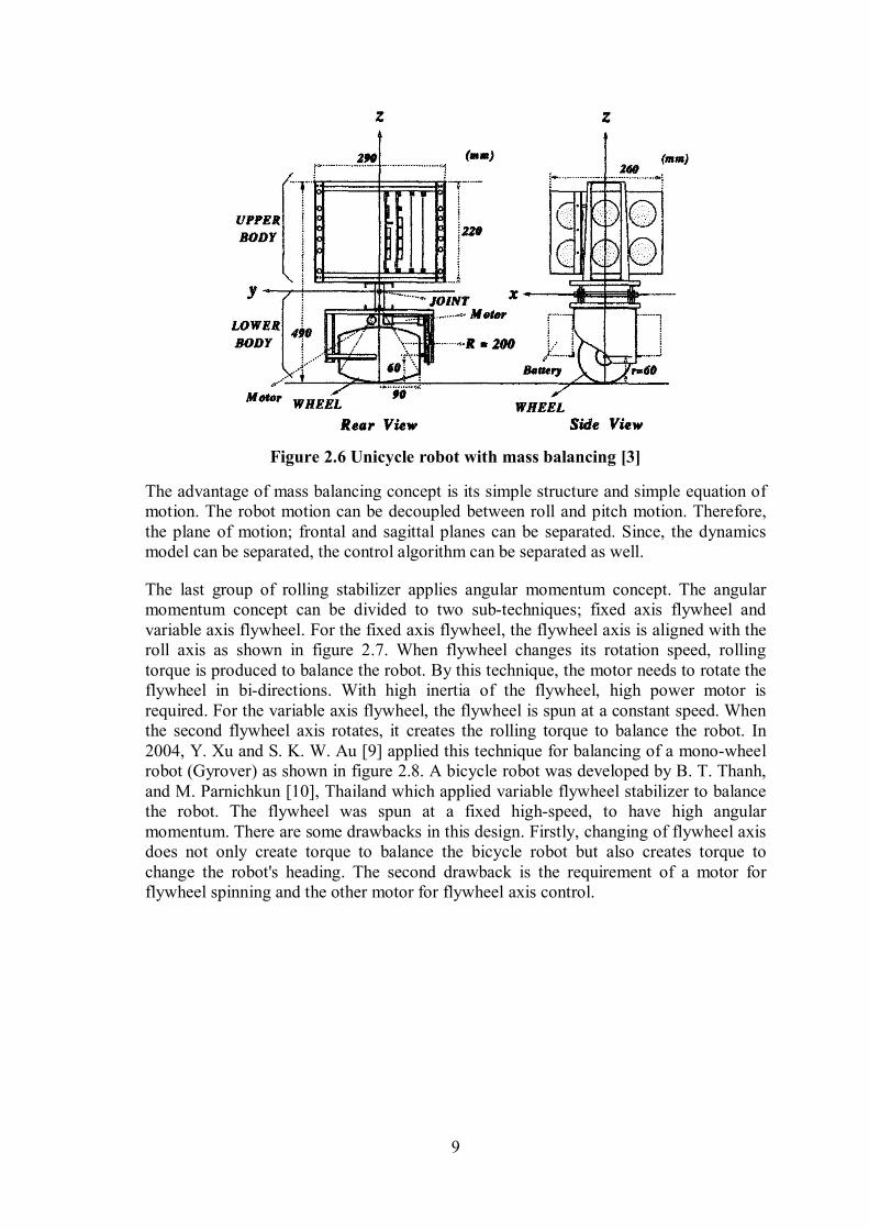
 Figure 2.6 Unicycle robot with mass balancing [3]

The advantage of mass balancing concept is its simple structure and simple equation of motion. The robot motion can be decoupled between roll and pitch motion. Therefore, the plane of  motion;  frontal and sagittal planes can  be  separated. Since,  the dynamics model can be separated, the control algorithm can be separated as well. 

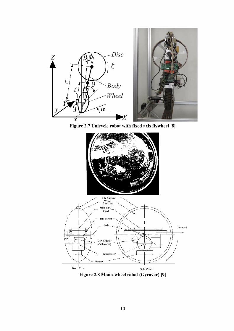
The  last  group  of  rolling  stabilizer  applies  angular  momentum  concept.  The  angular momentum  concept  can  be  divided  to  two  sub-techniques;  fixed  axis  flywheel  and variable axis flywheel. For the fixed axis flywheel, the flywheel axis is aligned with the roll  axis  as  shown  in  figure  2.7.  When  flywheel  changes  its  rotation  speed,  rolling torque is produced to balance the robot. By this technique, the motor needs to rotate the flywheel  in  bi-directions.  With  high  inertia  of  the  flywheel,  high  power  motor  is required. For the variable axis flywheel, the flywheel is spun at a constant speed. When the  second  flywheel  axis  rotates,  it  creates  the  rolling  torque  to  balance  the  robot.  In 2004, Y. Xu and S. K. W. Au [9] applied this technique for balancing of a mono-wheel robot (Gyrover) as shown in figure 2.8. A bicycle robot was developed by B. T. Thanh, and M. Parnichkun [10], Thailand which applied variable flywheel stabilizer to balance the  robot.  The  flywheel  was  spun  at  a  fixed  high-speed,  to  have  high  angular momentum. There are some drawbacks in this design. Firstly, changing of flywheel axis does  not  only  create  torque  to  balance  the  bicycle  robot  but  also  creates  torque  to change  the  robot's  heading.  The  second  drawback  is  the  requirement  of  a  motor  for flywheel spinning and the other motor for flywheel axis control.  

 

10  

 Figure 2.7 Unicycle robot with fixed axis flywheel [8]

 Figure 2.8 Mono-wheel robot (Gyrover) [9]

 

11  

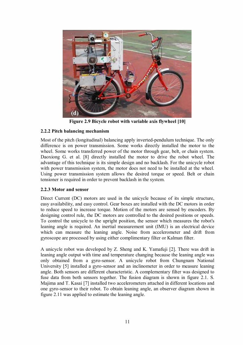
 Figure 2.9 Bicycle robot with variable axis flywheel [10]

2.2.2 Pitch balancing mechanism

Most of the pitch (longitudinal) balancing apply inverted-pendulum technique. The only difference  is  on  power  transmission.  Some  works  directly  installed  the  motor  to  the wheel. Some works transferred power of the motor through gear, belt, or chain system. Daoxiong  G.  et  al.  [8]  directly  installed  the  motor  to  drive  the  robot  wheel.  The advantage of this technique is its simple design and no backlash. For the unicycle robot with power transmission system,  the motor does not need to be  installed at  the wheel. Using  power  transmission  system  allows  the  desired  torque  or  speed.  Belt  or  chain tensioner is required in order to prevent backlash in the system. 

2.2.3 Motor and sensor

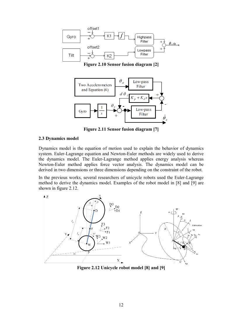
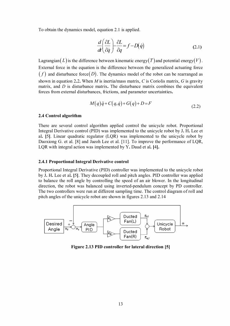
Direct  Current  (DC)  motors  are  used  in  the  unicycle  because  of  its  simple  structure, easy availability, and easy control. Gear boxes are installed with the DC motors in order to  reduce  speed  to  increase  torque.  Motion  of  the  motors  are  sensed  by  encoders. By designing control rule, the DC motors are controlled to the desired positions or speeds. To control  the unicycle  to the upright position,  the  sensor which  measures  the  robot's leaning  angle  is  required.  An  inertial  measurement  unit  (IMU)  is  an  electrical  device which  can  measure  the  leaning  angle.  Noise  from  accelerometer  and  drift  from gyroscope are processed by using either complimentary filter or Kalman filter.   A unicycle  robot was developed by Z. Sheng and K. Yamafuji  [2]. There was drift  in leaning angle output with time and temperature changing because the leaning angle was only  obtained  from  a  gyro-sensor.  A  unicycle  robot  from  Chungnam  National University  [5]  installed a gyro-sensor and an  inclinometer  in order  to measure  leaning angle. Both sensors are different characteristic. A complementary filter was designed to fuse  data  from  both  sensors  together.  The  fusion  diagram  is  shown  in  figure  2.1.  S. Majima and T. Kasai [7] installed two accelerometers attached in different locations and one gyro-sensor to their  robot. To obtain  leaning angle, an observer diagram shown  in figure 2.11 was applied to estimate the leaning angle.  

 

12  

 Figure 2.10 Sensor fusion diagram [2]

 

 Figure 2.11 Sensor fusion diagram [7]

2.3 Dynamics model

Dynamics  model  is  the  equation  of  motion  used  to  explain  the  behavior  of  dynamics system. Euler-Lagrange equation and Newton-Euler methods are widely used to derive the  dynamics  model.  The  Euler-Lagrange  method  applies  energy  analysis  whereas Newton-Euler  method  applies  force  vector  analysis.  The  dynamics  model  can  be derived in two dimensions or three dimensions depending on the constraint of the robot. 

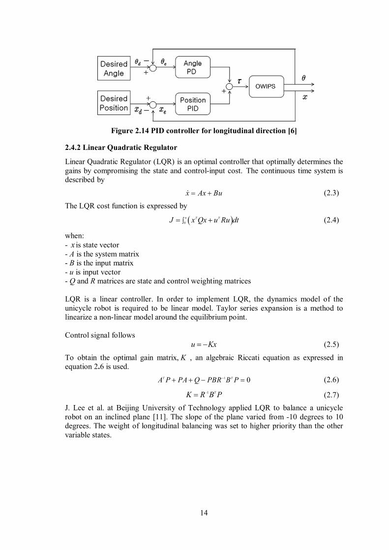
In  the previous works,  several  researchers of unicycle  robots used the Euler-Lagrange method to derive the dynamics model. Examples of  the robot model  in  [8] and [9] are shown in figure 2.12.  

 Figure 2.12 Unicycle robot model [8] and [9]

    

 

13  

To obtain the dynamics model, equation 2.1 is applied.   

  d L L

f D qdt q q

(2.1) 

Lagrangian L is the difference between kinematic energy T and potential energy V . 

External force in the equation is the difference between the generalized actuating force 

f  and disturbance force D . The dynamics model of the robot can be rearranged as 

shown in equation 2.2. When M is inertia/mass matrix, C is Coriolis matrix, G is gravity matrix,  and  D  is  disturbance  matrix. The  disturbance  matrix  combines  the  equivalent forces from external disturbances, frictions, and parameter uncertainties.  

  ,  M q q C q q G q D F

      (2.2) 

2.4 Control algorithm

There  are  several  control  algorithm  applied  control  the  unicycle  robot.  Proportional Integral Derivative control (PID) was implemented to the unicycle robot by J. H. Lee et al. [5].  Linear  quadratic  regulator  (LQR)  was  implemented  to  the  unicycle  robot  by Daoxiong G. et al. [8] and Jaeoh Lee et al. [11]. To improve the performance of LQR, LQR with integral action was implemented by Y. Daud et al. [4].   

2.4.1 Proportional Integral Derivative control

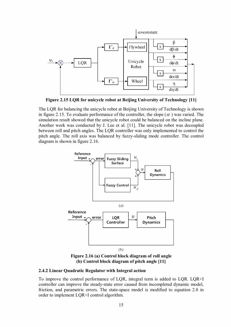
Proportional Integral Derivative (PID) controller was implemented to the unicycle robot by J. H. Lee et al. [5]. They decoupled roll and pitch angles. PID controller was applied to balance  the  roll  angle  by controlling  the speed of an air  blower. In  the  longitudinal direction,  the  robot  was  balanced  using  inverted-pendulum  concept  by  PD  controller. The two controllers were run at different sampling time. The control diagram of roll and pitch angles of the unicycle robot are shown in figures 2.13 and 2.14 

 Figure 2.13 PID controller for lateral direction [5]

 

14  

 Figure 2.14 PID controller for longitudinal direction [6]

2.4.2 Linear Quadratic Regulator

Linear Quadratic Regulator (LQR) is an optimal controller that optimally determines the gains by compromising  the state and control-input cost.  The continuous  time system  is described by 

  x Ax Bu            (2.3) 

The LQR cost function is expressed by 

0

T TJ x Qx u Ru dt

(2.4)

when: -  x is state vector - A is the system matrix - B is the input matrix - u is input vector - Q and R matrices are state and control weighting matrices  LQR  is  a  linear  controller.  In  order  to  implement  LQR,  the  dynamics  model  of  the unicycle  robot  is  required  to  be  linear  model. Taylor  series  expansion  is  a  method  to linearize a non-linear model around the equilibrium point.   Control signal follows   u Kx            (2.5) 

To  obtain  the  optimal  gain  matrix, K ,  an  algebraic  Riccati  equation as  expressed  in equation 2.6 is used. 

  1 0T TA P PA Q PBR B P        (2.6) 

1 TK R B P            (2.7)

J.  Lee  et  al.  at  Beijing  University  of  Technology  applied  LQR  to  balance  a  unicycle robot on an  inclined plane  [11]. The slope of  the plane varied  from -10 degrees to 10 degrees. The weight of  longitudinal balancing was set to higher priority than the other variable states.  

 

15  

 Figure 2.15 LQR for unicycle robot at Beijing University of Technology [11]

The LQR for balancing the unicycle robot at Beijing University of Technology is shown in figure 2.15. To evaluate performance of the controller, the slope ( ) was varied. The simulation result showed that the unicycle robot could be balanced on the incline plane.  Another work was conducted by J. Lee et al.  [11]. The unicycle  robot was decoupled between roll and pitch angles. The LQR controller was only implemented to control the pitch  angle. The  roll  axis was  balanced  by  fuzzy-sliding  mode  controller. The  control diagram is shown in figure 2.16.   

 Figure 2.16 (a) Control block diagram of roll angle

(b) Control block diagram of pitch angle [11]

2.4.2 Linear Quadratic Regulator with Integral action

To  improve  the  control  performance of  LQR,  integral  term  is  added  to  LQR. LQR+I controller can improve the steady-state error caused from incompleted dynamic model, friction,  and  parametric  errors.  The  state-space  model  is  modified  to  equation  2.8  in order to implement LQR+I control algorithm. 

 

16  

 

0  

0 0

   

e er

e er

x xx x A Bx u

z zx x C

Ax Bu

      (2.8) 

where: -   is error state

-   is 

-   is the reference input.

e

e

r

x

z edt

x

 

Controller gain of the LQR with Integral action is determined from an algebraic Riccati equation similar  to the LQR. The control signal follows 

  e

i r i r

e

xu Kx K K K x x K C x x dt

z

    (2.9) 

Y. Daud et al. developed a unicycle robot with mass moving technique to stabilize roll angle [4]. The LQR+I was applied to control all states of the robot; such as lateral angle, longitudinal angle, pendulum angle, turning angle, and wheel angle.  

2.4.3 Fuzzy Logic controller

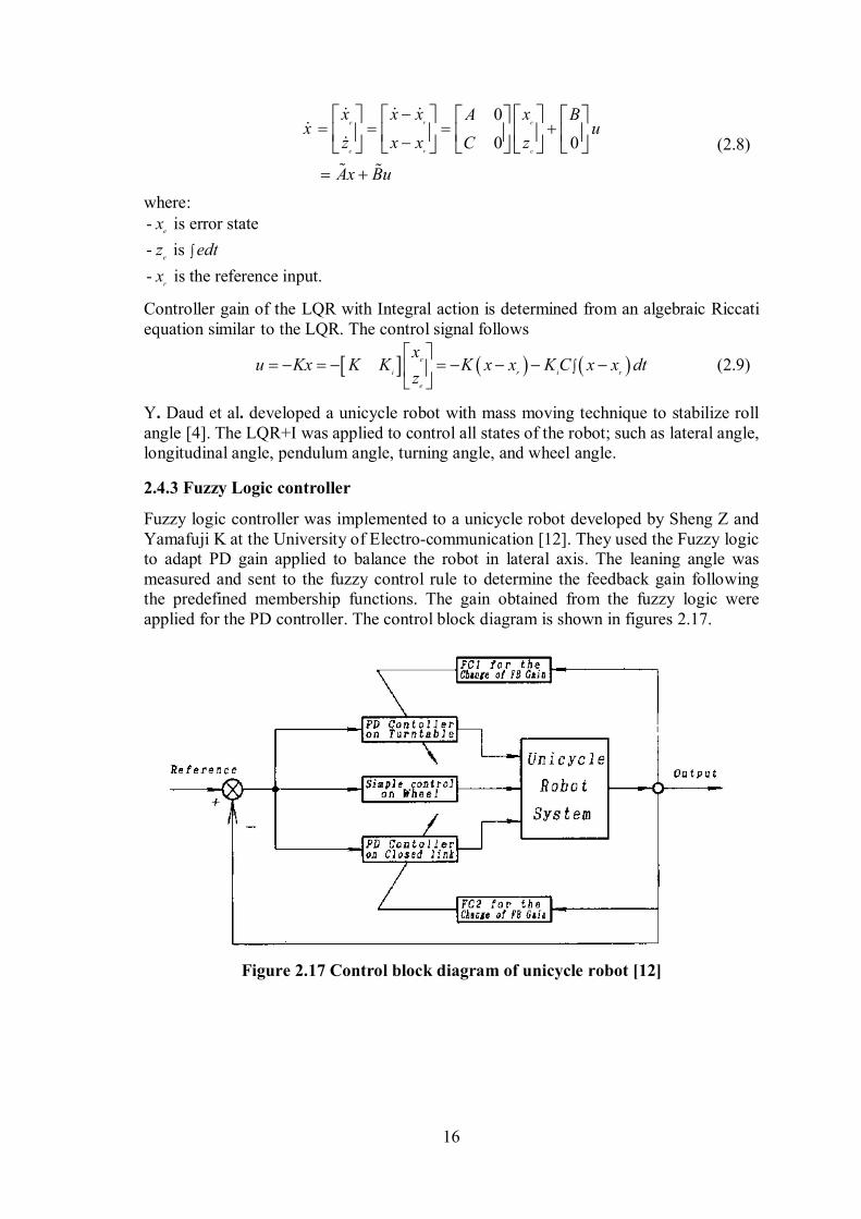
Fuzzy logic controller was implemented to a unicycle robot developed by Sheng Z and Yamafuji K at the University of Electro-communication [12]. They used the Fuzzy logic to  adapt  PD  gain  applied  to  balance  the  robot  in  lateral  axis.  The  leaning  angle  was measured and sent  to the  fuzzy control  rule  to determine  the  feedback gain  following the  predefined  membership  functions.  The  gain  obtained  from  the  fuzzy  logic  were applied for the PD controller. The control block diagram is shown in figures 2.17.  

 Figure 2.17 Control block diagram of unicycle robot [12]

   

 

17  

CHAPTER 3 UNICYCLE ROBOT HARDWARE

3.1 Conceptual design

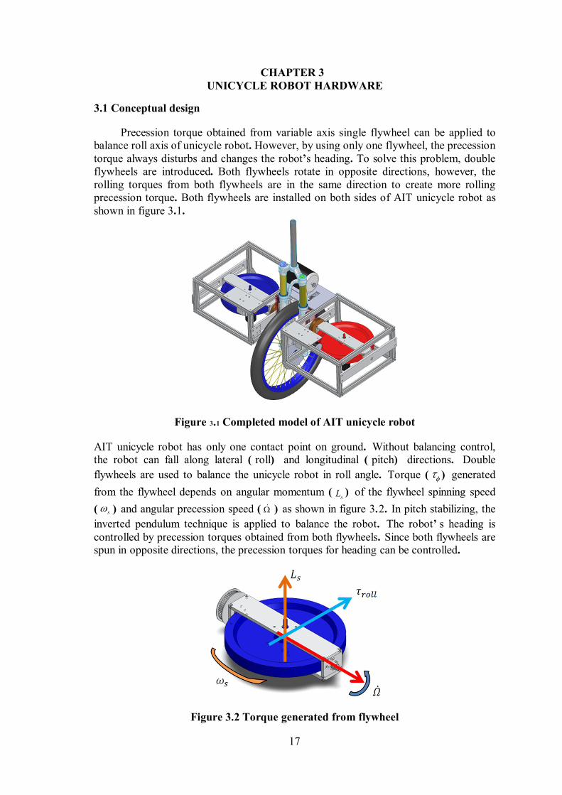
Precession  torque obtained  from  variable  axis  single  flywheel  can  be  applied  to balance roll axis of unicycle robot. However, by using only one flywheel, the precession torque always disturbs and changes the robot’s heading. To solve this problem, double flywheels  are  introduced. Both  flywheels  rotate  in  opposite  directions,  however, the rolling  torques  from  both  flywheels  are  in  the  same  direction  to  create  more  rolling precession torque. Both flywheels are  installed on both sides of AIT unicycle robot as shown in figure 3.1.  

Figure �.� Completed model of AIT unicycle robot

AIT  unicycle  robot  has  only  one  contact  point  on  ground. Without  balancing  control, the  robot  can  fall  along  lateral  ( roll) and  longitudinal  ( pitch) directions. Double 

flywheels  are  used  to  balance  the  unicycle  robot  in  roll  angle. Torque  ( ) generated 

from  the  flywheel depends on  angular momentum  (sL ) of  the  flywheel  spinning  speed  

( s ) and angular precession speed ( ) as shown in figure 3.2. In pitch stabilizing, the 

inverted  pendulum  technique  is  applied  to  balance  the  robot. The  robot’ s  heading  is controlled by precession torques obtained from both flywheels. Since both flywheels are spun in opposite directions, the precession torques for heading can be controlled. 

Figure 3.2 Torque generated from flywheel

 

18  

3.1.1 Motor calculation

There are two main parts of  the unicycle robot: flywheel and driving wheel. The size, weight and spinning speed of the flywheels are designed to carry all the weight of the robot.  

Flywheel motor calculation

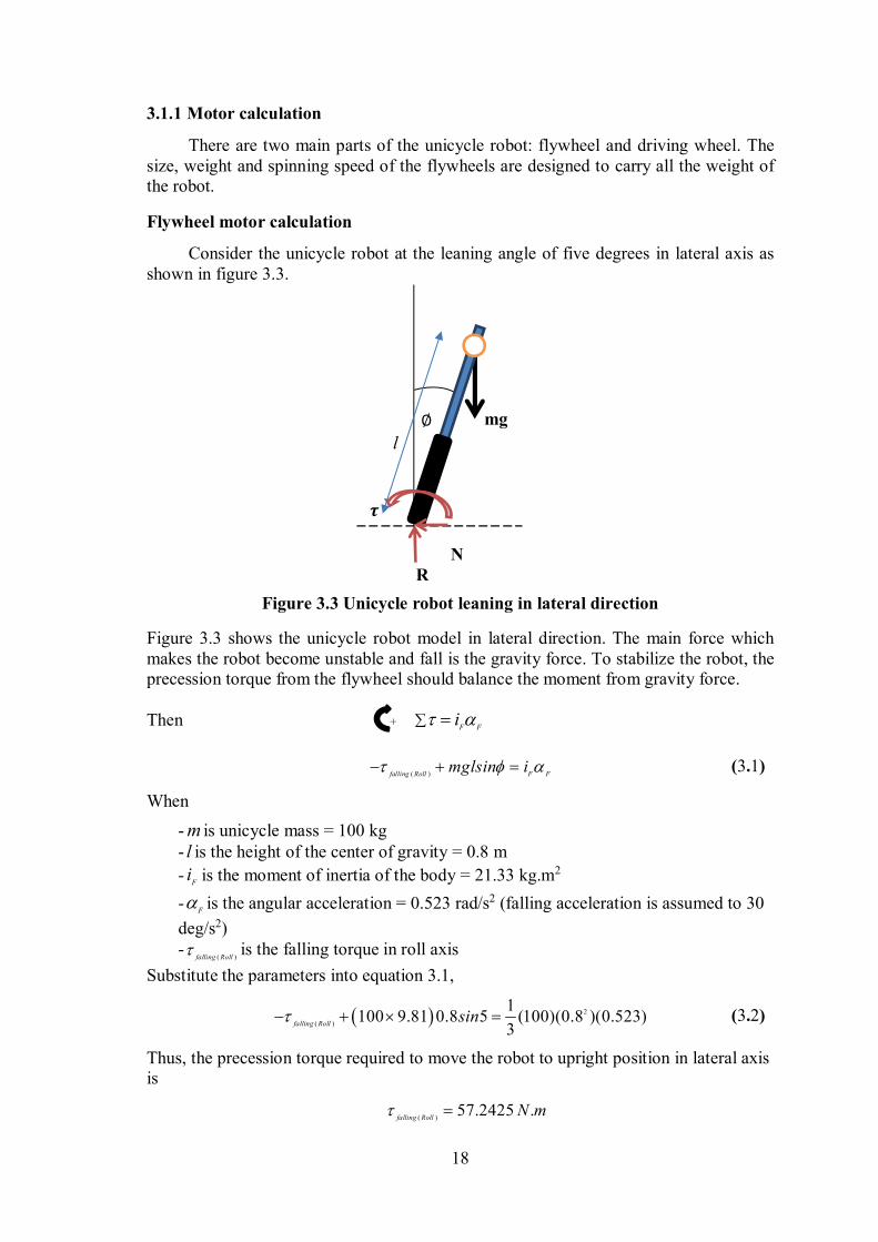
Consider the unicycle robot at the leaning angle of  five degrees  in  lateral axis as shown in figure 3.3. 

 Figure 3.3 Unicycle robot leaning in lateral direction 

Figure  3.3  shows  the  unicycle  robot  model  in  lateral  direction. The  main  force  which makes the robot become unstable and fall is the gravity force. To stabilize the robot, the precession torque from the flywheel should balance the moment from gravity force. 

Then         F F

i  

  

( )falling Roll F Fmglsin i         (3.1) 

When 

- m is unicycle mass = 100 kg - l is the height of the center of gravity = 0.8 m 

-F

i is the moment of inertia of the body = 21.33 kg.m2 

-F is the angular acceleration = 0.523 rad/s2 (falling acceleration is assumed to 30 

deg/s2) -

( )falling Roll is the falling torque in roll axis 

Substitute the parameters into equation 3.1, 

  2

( )

1100 9.81 0.8 5 (100)(0.8 )(0.523)

3falling Roll

sin     (3.2) 

Thus, the precession torque required to move the robot to upright position in lateral axis is  

( )57.2425  .

falling RollN m  

�

N R

mg ∅

+

l

 

19  

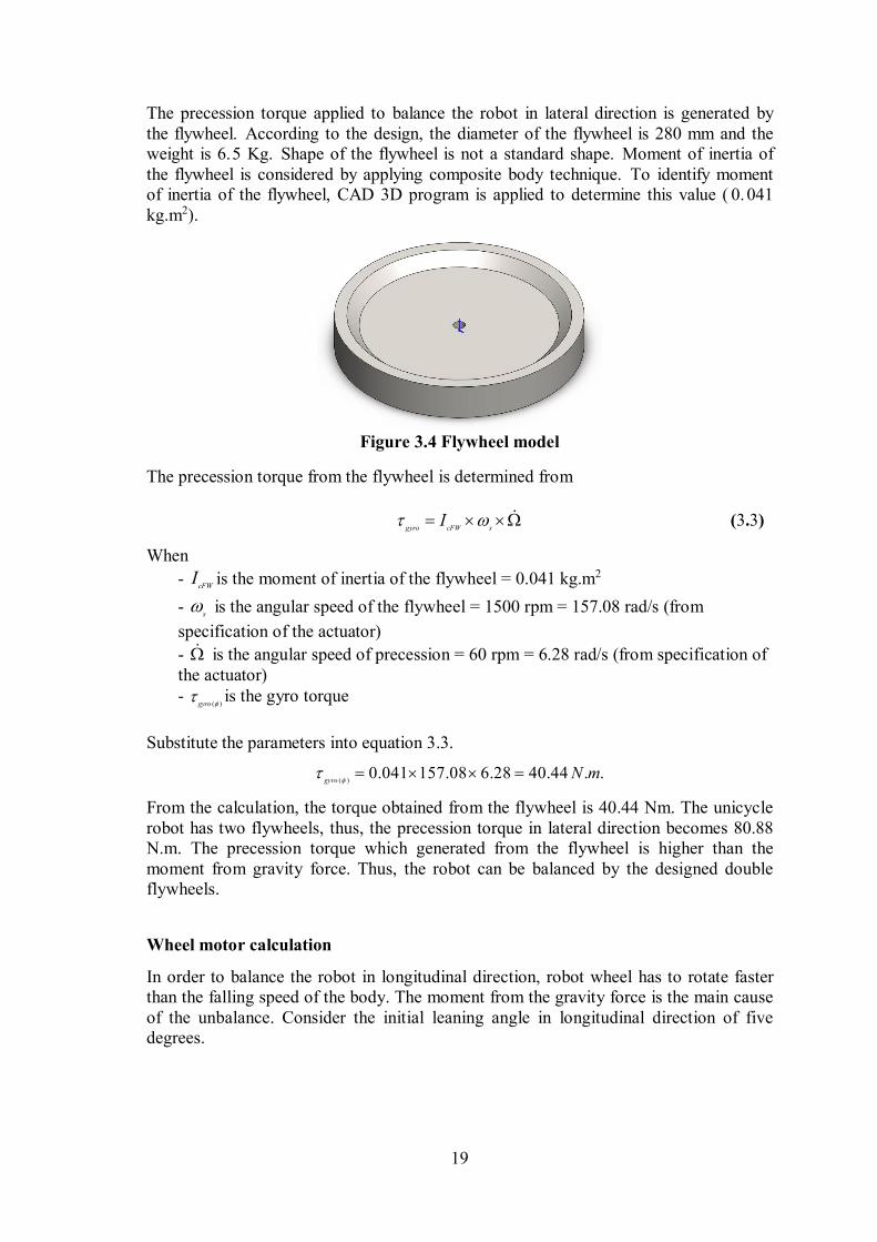
The  precession  torque  applied  to  balance  the  robot  in  lateral  direction  is  generated  by the flywheel.  According  to the design,  the diameter of  the  flywheel  is 280 mm and  the weight  is 6.5 Kg. Shape of  the  flywheel  is not a  standard  shape. Moment of  inertia of the  flywheel  is  considered  by applying  composite  body  technique.   To  identify  moment of  inertia  of  the  flywheel,  CAD  3D program  is  applied  to determine  this value  ( 0. 041 kg.m2). 

 Figure 3.4 Flywheel model

The precession torque from the flywheel is determined from  

 gyro cFW s

I         (3.3) 

When  

- cFW

I is the moment of inertia of the flywheel = 0.041 kg.m2  

- s  is the angular speed of the flywheel = 1500 rpm = 157.08 rad/s (from 

specification of the actuator) 

-   is the angular speed of precession = 60 rpm = 6.28 rad/s (from specification of the actuator) - 

( )gyro is the gyro torque  

 Substitute the parameters into equation 3.3.  

( )0.041 157.08 6.28 40.44  . .

gyroN m

 

From the calculation, the torque obtained from the flywheel  is 40.44 Nm. The unicycle robot has two flywheels,  thus, the precession torque in  lateral direction becomes 80.88 N.m.  The  precession  torque  which  generated  from  the  flywheel  is  higher  than  the moment  from  gravity  force.  Thus,  the  robot  can  be  balanced  by  the  designed  double flywheels.  

Wheel motor calculation

In order to balance the robot  in  longitudinal direction, robot wheel has to rotate faster than the falling speed of the body. The moment from the gravity force is the main cause of  the  unbalance.  Consider  the  initial  leaning  angle  in  longitudinal  direction  of  five degrees.  

 

20  

  

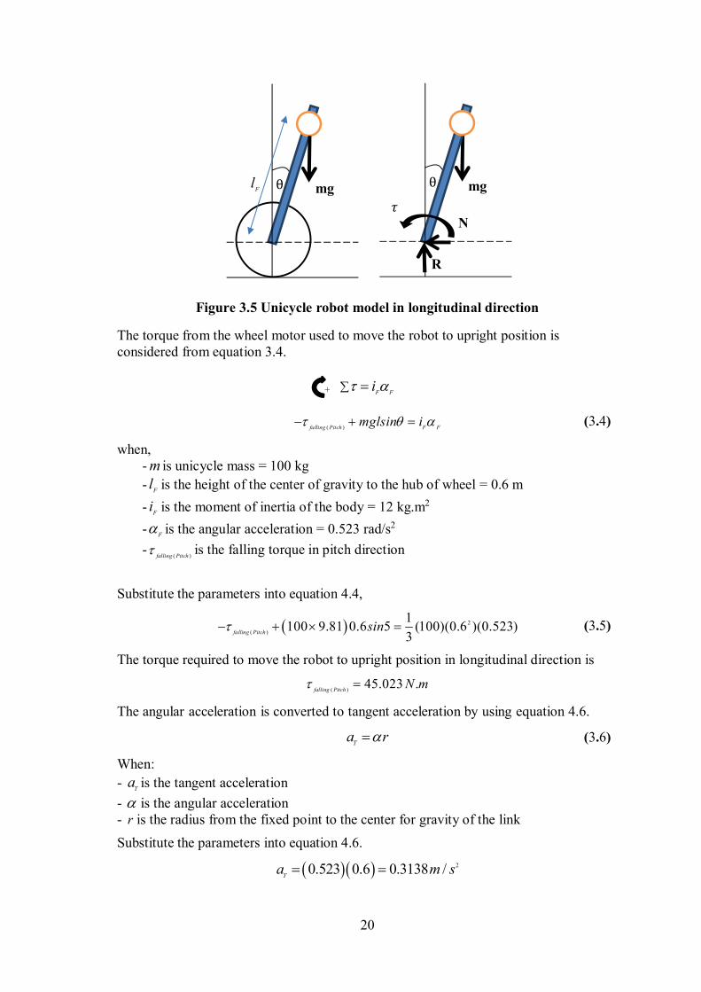
Figure 3.5 Unicycle robot model in longitudinal direction 

The torque from the wheel motor used to move the robot to upright position is considered from equation 3.4.  

F Fi  

 ( )falling Pitch F F

mglsin i         (3.4) 

when,  - m is unicycle mass = 100 kg 

-F

l is the height of the center of gravity to the hub of wheel = 0.6 m 

-F

i is the moment of inertia of the body = 12 kg.m2 

-F is the angular acceleration = 0.523 rad/s2 

-( )falling Pitch

is the falling torque in pitch direction 

 

Substitute the parameters into equation 4.4, 

  2

( )

1100 9.81 0.6 5 (100)(0.6 )(0.523)

3falling Pitch

sin     (3.5) 

The torque required to move the robot to upright position in longitudinal direction is  

( )45.023  .

falling PitchN m  

The angular acceleration is converted to tangent acceleration by using equation 4.6. 

 T

a r            (3.6) 

When:  

- T

a is the tangent acceleration 

-  is the angular acceleration -  r is the radius from the fixed point to the center for gravity of the link 

Substitute the parameters into equation 4.6.  

20.523 0.6 0.3138  /T

a m s  

θ mg

� N

R

θ mg

+

Fl

 

21  

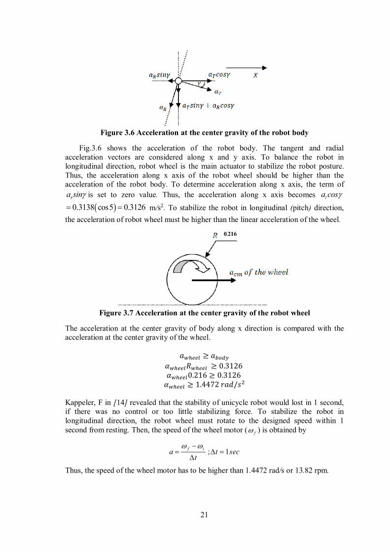
 Figure 3.6 Acceleration at the center gravity of the robot body

Fig.3.6  shows  the  acceleration  of  the  robot  body.  The  tangent  and  radial acceleration  vectors  are  considered  along  x  and  y  axis.  To  balance  the  robot  in longitudinal  direction,  robot  wheel  is  the  main  actuator  to  stabilize  the  robot  posture. Thus,  the  acceleration  along  x  axis  of  the  robot  wheel  should  be  higher  than  the acceleration  of  the  robot  body.  To  determine  acceleration  along  x  axis,  the  term  of 

Ra sin is  set  to  zero  value. Thus,  the  acceleration  along  x  axis  becomes 

Ta cos

0.3138 cos5 0.3126 m/s2. To stabilize  the  robot  in  longitudinal  (pitch) direction, 

the acceleration of robot wheel must be higher than the linear acceleration of the wheel.  

 Figure 3.7 Acceleration at the center gravity of the robot wheel

The  acceleration  at  the  center  gravity  of  body  along  x  direction  is  compared  with  the acceleration at the center gravity of the wheel.  

������ ≥ �����

������������ ≥ 0.3126 ������0.216 ≥ 0.3126

������ ≥ 1.4472 ���/��  Kappeler, F in [14] revealed that the stability of unicycle robot would lost in 1 second, if  there  was  no  control  or  too  little  stabilizing  force. To  stabilize the  robot  in longitudinal  direction,  the  robot  wheel  must  rotate  to  the  designed  speed  within  1 second from resting. Then, the speed of the wheel motor ( f ) is obtained by  

 ;  1 f i

a t sect

 

Thus, the speed of the wheel motor has to be higher than 1.4472 rad/s or 13.82 rpm. 

0.216

 

22  

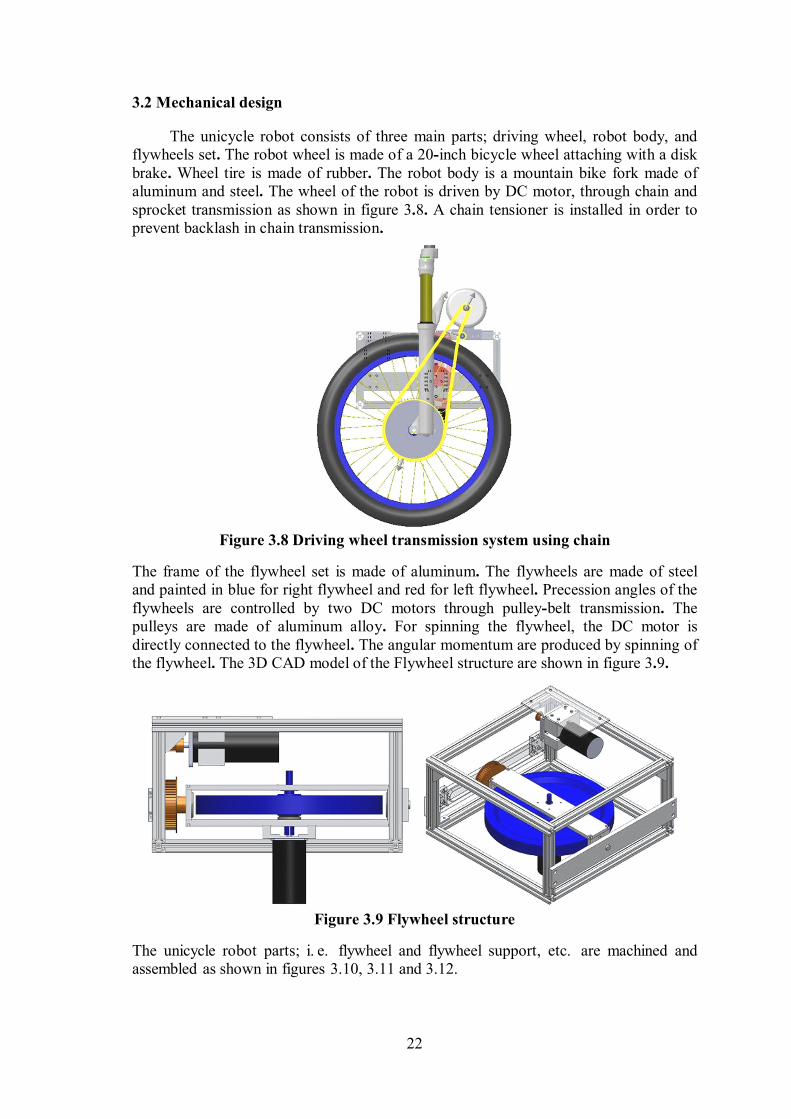
3.2 Mechanical design

The  unicycle  robot  consists  of  three  main  parts;  driving  wheel,  robot  body,  and flywheels set. The robot wheel is made of a 20-inch bicycle wheel attaching with a disk brake. Wheel  tire  is made of  rubber. The robot body  is a mountain  bike  fork made of aluminum and steel. The wheel of the robot is driven by DC motor, through chain and sprocket transmission as shown  in  figure 3.8. A chain tensioner  is  installed  in order to prevent backlash in chain transmission. 

 Figure 3.8 Driving wheel transmission system using chain

The  frame  of  the  flywheel  set  is  made of  aluminum. The  flywheels  are  made of  steel and painted in blue for right flywheel and red for left flywheel. Precession angles of the flywheels  are  controlled  by  two  DC  motors  through  pulley-belt  transmission. The pulleys  are  made  of  aluminum  alloy. For  spinning  the  flywheel,  the  DC  motor  is directly connected to the flywheel. The angular momentum are produced by spinning of the flywheel. The 3D CAD model of the Flywheel structure are shown in figure 3.9. 

 Figure 3.9 Flywheel structure 

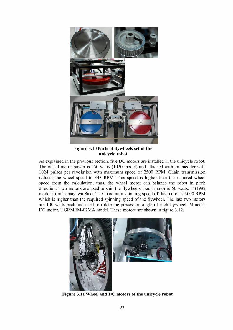
The  unicycle  robot  parts;  i. e.   flywheel  and  flywheel  support,  etc.   are  machined  and assembled as shown in figures 3.10, 3.11 and 3.12.  

 

23  

As explained in the previous section, five DC motors are installed in the unicycle robot. The wheel motor power is 250 watts (1020 model) and attached with an encoder with 1024  pulses  per  revolution  with  maximum  speed  of  2500  RPM.  Chain  transmission reduces  the  wheel  speed  to  343  RPM.  This  speed  is  higher  than  the  required  wheel speed  from  the  calculation,  thus,  the  wheel  motor  can  balance  the  robot  in  pitch direction. Two motors are used to spin the flywheels. Each motor  is 60 watts: TS1982 model from Tamagawa Saki. The maximum spinning speed of this motor is 3000 RPM which  is higher  than the required spinning speed of  the  flywheel. The  last  two motors are 100 watts each and used  to  rotate the precession angle of each  flywheel: Minertia DC motor, UGRMEM-02MA model. These motors are shown in figure 3.12.  

Figure 3.11 Wheel and DC motors of the unicycle robot 

Figure 3.10 Parts of flywheels set of the unicycle robot

 

24  

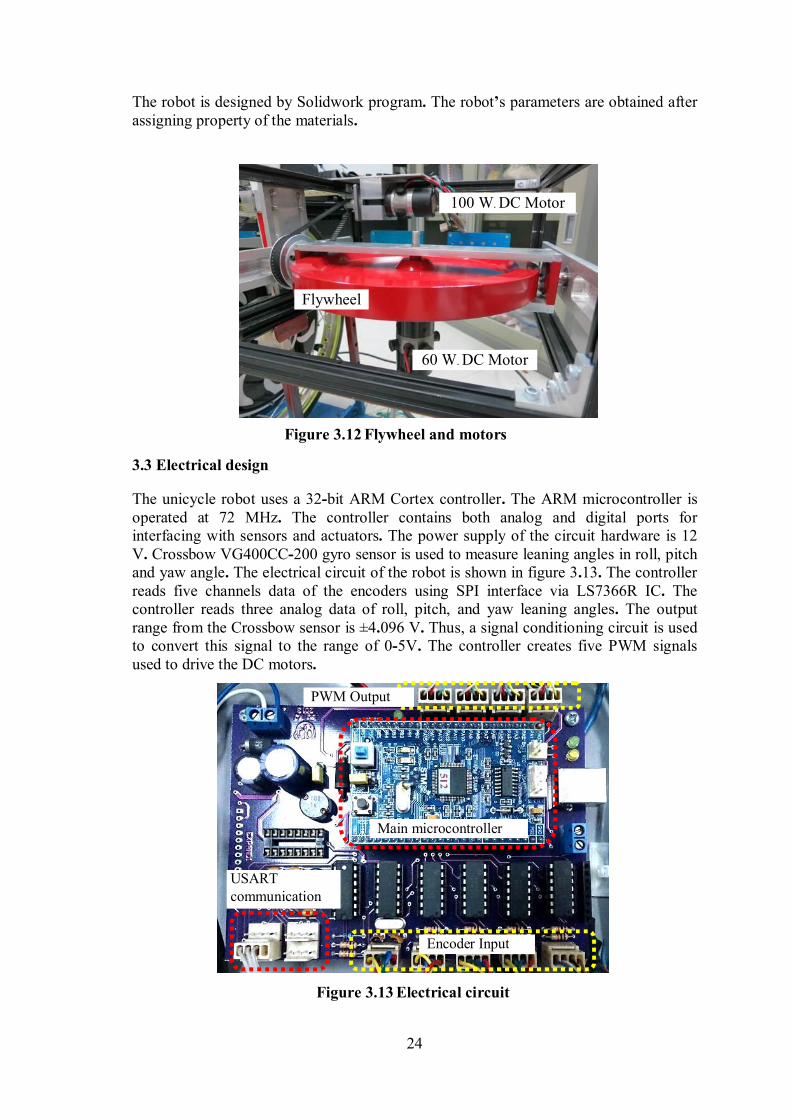
The robot is designed by Solidwork program. The robot’s parameters are obtained after assigning property of the materials.  

3.3 Electrical design

The unicycle robot uses a 32-bit ARM Cortex controller. The ARM microcontroller  is operated  at  72  MHz. The  controller  contains  both  analog  and  digital  ports  for interfacing with sensors and actuators. The power supply of  the circuit hardware  is 12 V. Crossbow VG400CC-200 gyro sensor is used to measure leaning angles in roll, pitch and yaw angle. The electrical circuit of the robot is shown in figure 3.13. The controller reads  five  channels  data  of  the  encoders  using  SPI  interface  via  LS7366R  IC. The controller  reads  three  analog  data  of  roll,  pitch,  and  yaw  leaning  angles. The  output range from the Crossbow sensor is ±4.096 V. Thus, a signal conditioning circuit is used to  convert  this  signal  to  the  range  of  0-5V. The  controller  creates  five  PWM  signals used to drive the DC motors. 

  Encoder Input 

 USART  communication 

  Main microcontroller 

  PWM Output 

Figure 3.13 Electrical circuit

Flywheel 

100 W. DC Motor 

60 W. DC Motor 

Figure 3.12 Flywheel and motors 

 

25  

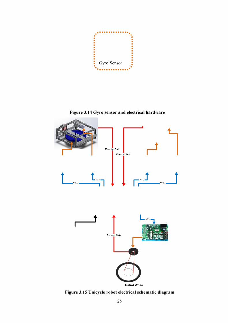
 Figure 3.15 Unicycle robot electrical schematic diagram

  Gyro Sensor 

Figure 3.14 Gyro sensor and electrical hardware

 

26  

The unicycle robot electrical schematic diagram is shown in figure 3.15. All of the data; such  as  position  of  each  motor  and  leaning  angle  of  the  robot,  are  fed  back  to  the microcontroller and shown in red line. The output of the controller are the Pulse Width Modulation  (PWM)  signal  shown  in  the  blue  line.  The  output  signals  are  sent  to  the motor drivers for power amplification before forwarding to the DC motors.  

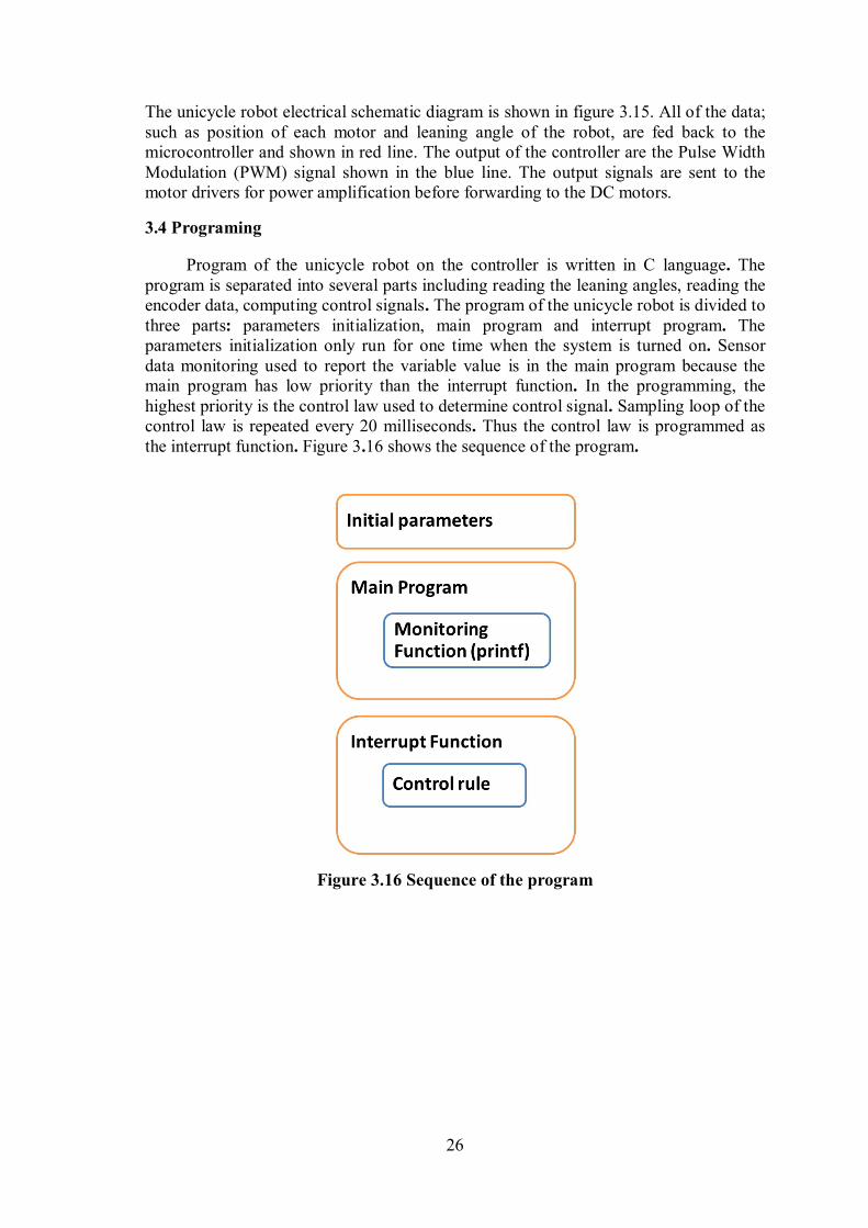
3.4 Programing

Program  of  the  unicycle  robot  on  the  controller  is  written  in  C  language. The program is separated into several parts including reading the leaning angles, reading the encoder data, computing control signals. The program of the unicycle robot is divided to three  parts: parameters initialization,  main  program  and  interrupt  program. The parameters  initialization  only  run  for  one  time  when  the  system  is  turned  on. Sensor data monitoring  used  to  report  the  variable  value  is  in  the  main  program  because  the main  program has  low  priority  than  the  interrupt  function. In  the  programming,  the highest priority is the control law used to determine control signal. Sampling loop of the control  law  is  repeated every 20 milliseconds. Thus  the control  law  is programmed as the interrupt function. Figure 3.16 shows the sequence of the program.  

 

Figure 3.16 Sequence of the program

 

 

 

27  

CHAPTER 4 DYNAMIC MODEL

The  unicycle  robot  dynamic  model  is  derived  from  two  separated  subsystems, unicycle wheel and robot body. The Euler-Lagrange equation is applied for deriving the unicycle  robot  dynamic  model.  All  friction  in  the  unicycle  robot  model  is  assumed small and negligible.  

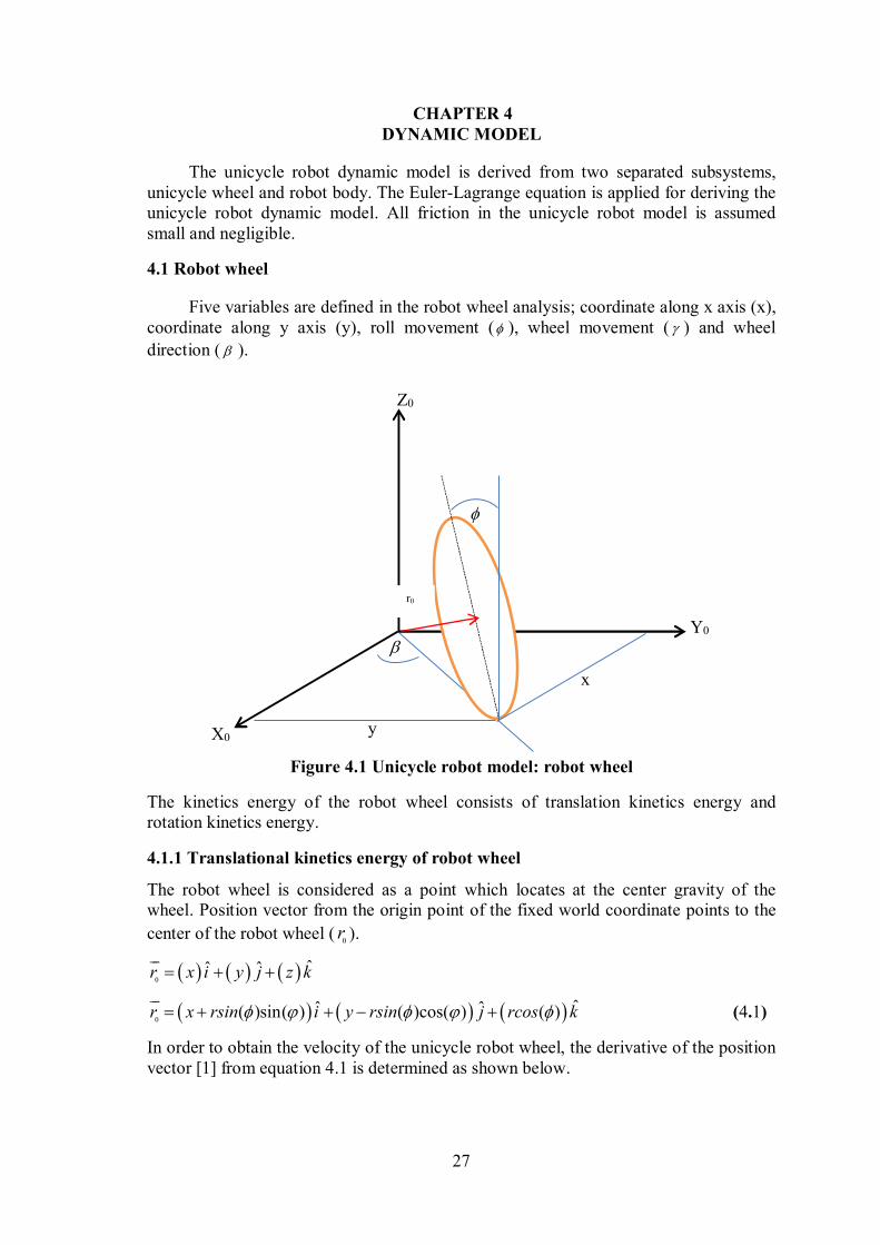
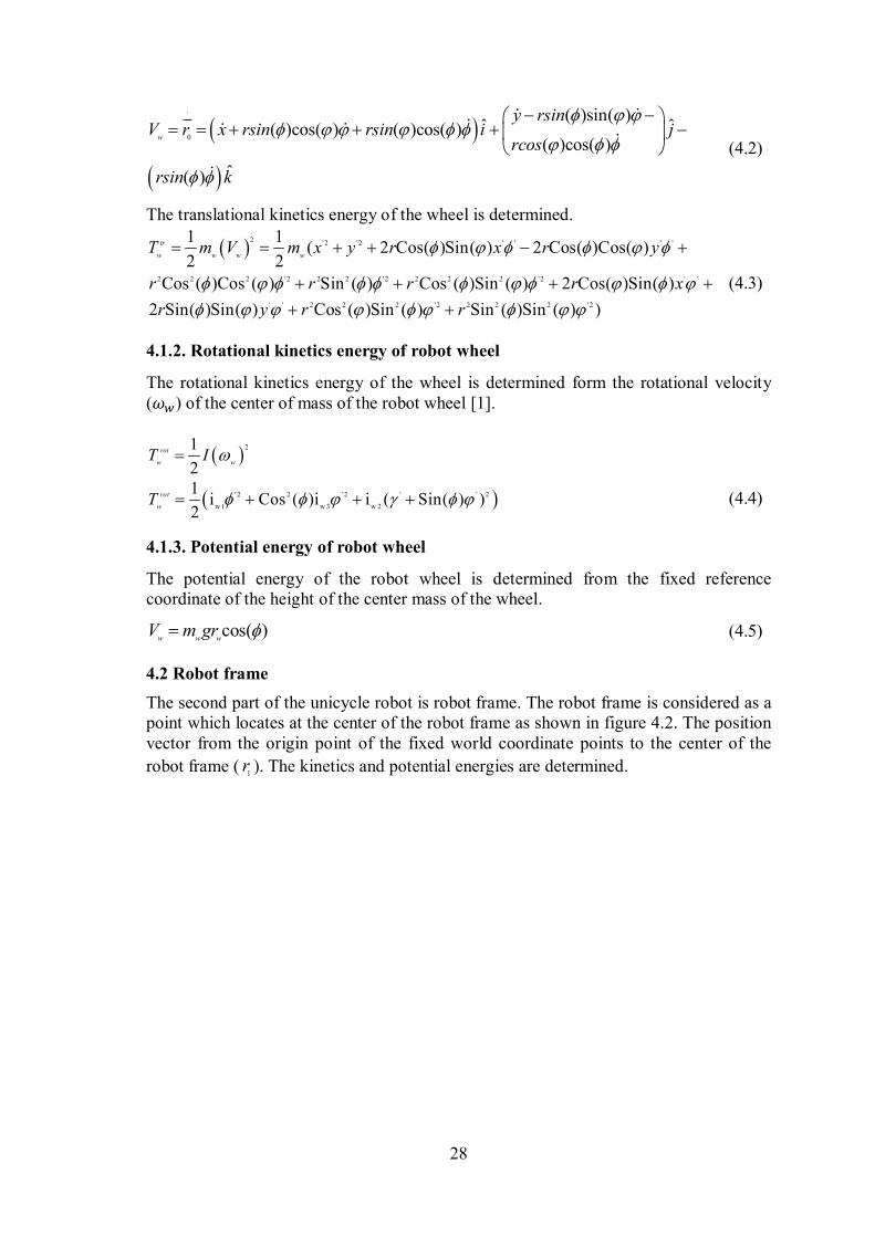
4.1 Robot wheel

Five variables are defined in the robot wheel analysis; coordinate along x axis (x), coordinate  along  y  axis  (y),  roll  movement  ( ),  wheel  movement  ( )  and  wheel 

direction ( ).  

 

 Figure 4.1 Unicycle robot model: robot wheel

The  kinetics  energy  of  the  robot  wheel  consists  of  translation  kinetics  energy  and rotation kinetics energy. 

4.1.1 Translational kinetics energy of robot wheel

The  robot  wheel  is  considered  as  a  point  which  locates  at  the  center  gravity  of  the wheel. Position vector from the origin point of the fixed world coordinate points to the 

center of the robot wheel (0

r ). 

0ˆ ˆ ˆr x i y j z k

 

0( )sin( ˆˆ ˆ) ( )cos( ) ( )r x rsin i y rsin j rcos k

      (4.1) 

In order to obtain the velocity of the unicycle robot wheel, the derivative of the position vector [1] from equation 4.1 is determined as shown below. 

Z0 

X0 

Y0 

y 

x 

r0 

 

28  

˙

0

( )sin( )( )cos( ) ( )cos( )

( )cos( )

(

ˆ

)

ˆ

ˆ

w

y rsinV r x rsin rsin i j

rcos

rsin k

  (4.2) 

The translational kinetics energy of the wheel is determined. 

2 '2 '2 ' ' ' '

2 2 2 '2 2 2 '2 2 2 2 '2 ' '

' ' 2 2 2 '2 2 2 2 '2

1 1( 2 Cos( )Sin( ) 2 Cos( )Cos( )

2 2

Cos ( )Cos ( ) Sin ( ) Cos ( )Sin ( ) 2 Cos( )Sin( )

2 Sin( )Sin( ) Cos ( )Sin ( ) Sin ( )Sin ( ) )

tr

w w w wT m V m x y r x r y

r r r r x

r y r r

  (4.3) 

4.1.2. Rotational kinetics energy of robot wheel

The  rotational  kinetics  energy  of  the  wheel  is  determined  form  the  rotational  velocity (��) of the center of mass of the robot wheel [1].  

21

2rot

w wT I  

' 2 2 '2 ' ' 2

w1 w 3 w 2

1i Cos ( )i i ( Sin( ) )

2rot

wT           (4.4) 

4.1.3. Potential energy of robot wheel

The  potential  energy  of  the  robot  wheel  is  determined  from  the  fixed  reference coordinate of the height of the center mass of the wheel. 

cos( )w w w

V m gr                   (4.5) 

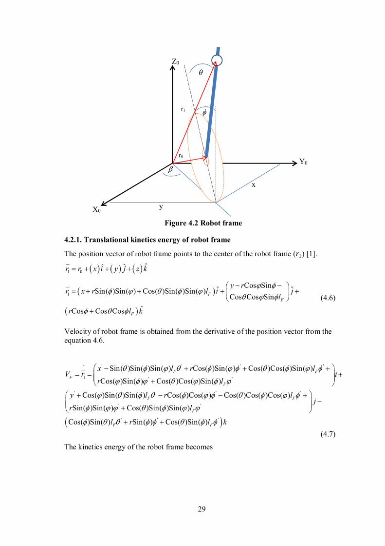
4.2 Robot frame

The second part of the unicycle robot is robot frame. The robot frame is considered as a point which locates at the center of the robot frame as shown in figure 4.2. The position vector  from  the  origin  point  of  the  fixed  world  coordinate  points  to  the  center of  the 

robot frame (1r ). The kinetics and potential energies are determined. 

 

29  

4.2.1. Translational kinetics energy of robot frame

The position vector of robot frame points to the center of the robot frame (��) [1]. 

1 0ˆˆ ˆr r x i y j z k

 

1

Cos SinSin( )Sin( ) Cos( )Sin( )Sin( )

Cos Cos Sin

Cos C

ˆ ˆ

ˆos Cos

F

F

F

y rr x r l i j

l

r l k

  (4.6) 

 Velocity of robot frame is obtained from the derivative of the position vector from the equation 4.6.  

 

' ' ' '˙

1 ' '

' ' ' '

Sin( )Sin( )Sin( ) Cos( )Sin( ) Cos( )Cos( )Sin( )

Cos( )Sin( ) Cos( )Cos( )Sin( )

Cos( )Sin( )Sin( ) Cos( )Cos( ) Cos( )Cos( )Cos( )

Sin( )Sin( )

F F

F

F

F F

x l r lV r i

r l

y l r l

r

' '

' ' '

Cos( )Sin( )Sin( )

Cos( )Sin( ) Sin( ) Cos( )Sin( )

F

F F

jl

l r l k

                      (4.7) 

The kinetics energy of the robot frame becomes 

Z0 

X0 

Y0 

y 

x 

r0 

�

r1 

Figure 4.2 Robot frame

 

30  

2' ' ' '

' '

' ' ' '

Sin( )Sin( )Sin( ) Cos( )Sin( ) Cos( )Cos( )Sin( )

Cos( )Sin( ) Cos( )Cos( )Sin( )

Cos( )Sin( )Sin( ) Cos( )Cos( ) Cos( )Cos( )Cos( )1

2 Sin( )Sin( )

F F

F

F FtrF F

x l r l

r l

y l r lT m

r

2

' '

2' ' '

Cos( )Sin( )Sin( )

Cos( )Sin( ) Sin( ) Cos( )Sin( )

F

F F

l

l r l

                        (4.8) 

4.2.2. Rotational kinetics energy of robot frame

The rotational kinetics energy of robot frame is determined form the rotational velocity  

(F ) of the center of mass of the robot frame [1].

21

2rot

F FT I                   (4.9) 

' ' 2 ' ' 2 ' ' 2F3 F1 F2

1 1 1i (Sin Cos Cos ) i (Cos Cos Sin ) i ( Sin )

2 2 2rot

FT  

(4.10) 

4.2.3. Potential energy of robot frame

The potential energy of robot frame is determined from the fixed reference coordinate of the height of the center mass of the robot frame. 

F F w FV m g r cos l cos cos               (4.11) 

The summation of kinetics energy of the unicycle robot is expressed in equation 4.12.  

2 2 2 2 2 2 2w2 F2 F1 F3 w1 w2

2 2 2F2 F1 F3 F1

0.5 0.5 0.5 os ( ) 0.5sin ( ) 0.5 sin( )

sin( ) cos( )cos( )sin( ) cos( )cos( )sin( ) 0.5cos ( )sin ( )

0.5si

tr rot tr rotw w F FT T T T

i i c i i i i

i i i i

T

T

2 2 2 2 2 2 2 2 2 2 2

2

2 2 2 2 2 2 2 2 2

F2 F3 w2 w3

0.5 0.5 0.5 0.5 cos( ) 0.25 0.25cos(2 )

0.5 sin( ) 0.5 sin( ) sin( ) 0

n ( ) 0.5cos ( )cos ( ) 0.5sin ( ) 0.5cos ( )

F F F F

F F F

F

x y l r r l l l

r l r l l

m

i i i i

2 2 2 2

2 2 2 2

2 2 2 2 2

.5 sin( )

0.5 sin( ) 0.25sin(2 ) 0.25sin(2 ) 0.25

0.25 cos(2 ) 0.5 cos( ) 0.25 cos( 2 )

0.25 cos( 2 ) 0.375 0.125cos(2 ) 0.0625c

F

F F F

F F

F F F

r l

r l l l r

r r l r l

r l l l

2 2

2 2 2 2

os 2( )

0.125cos(2 ) 0.0625cos 2( )

F

F F

l

l l

 

 

31  

cos( )cos( ) sin( )sin( )sin( )

cos( )sin( ) cos( )sin( ) cos( )cos( )sin( )

cos( )cos( )sin( ) sin( )sin( )

cos( )sin( )s

cos( )cos( ) in( )sin( )

F

F

F

x r l

m

y r rs l

in( ) cos( ) in( )

cos( )cos( )cos( )

cos( )sin( ) cos( )sin( )sin( )

s

 

2 2

2 2 2 2

0.5 0.5 cos( )sin( ) cos( )sin( ) cos( )cos( ) sin( )sin( )

0.5 0.5sin ( )w

x y rx rym

r

 

(4.12) 

The summation of potential energy of the unicycle robot is expressed in equation 4.13.  

cos( ) cos( )cos      ( ) cos( )

w F

F F w

V V V

g r l m gr m

        (4.13) 

where: -  is the roll angle measured around x axis  

-  is the yaw angle measured around z axis 

-  is the pitch angle measured around y axis -  is the robot wheel angle 

-1 2 3, ,

F F Fi i i  are the moments of inertia of the robot frame  

-1 2 3, ,

w w wi i i  are the moments of inertia of the robot wheel 

- r is the radius of the wheel 

-F

l is the length from robot frame to wheel hub of the unicycle robot (center gravity to 

center gravity)  

-w

m is the wheel mass 

-F

m is the frame mass 

4.3 Lagrangian and lagrange equation

Lagrange  equation  is  an  equation  that  describes  the  dynamics  system  using  energy concept.  Lagrangian  ( L )  is  the  difference  between  kinetic  energy  (T )  and  potential 

energy (V ) as L K P . Lagrange equation is expressed in equation 4.14 when the friction is small and neglected.  

 d L L

fdt q q

        (4.14) 

Where: - [ , , , ]Tq  

- f is the generalized forces. 

  

 

32  

From the Lagrange equation, there are four equations which define the dynamic model. The first equation is acquired from the derivation of roll direction ( ).  

2 2

F1 F3 w2 F1 F1

2 2 2

F2 F3 F3 F1

2 cos( )sin( ) 2 cos( )sin( ) cos( ) cos ( )cos( ) sin ( )cos( )

cos( ) cos ( )cos( ) cos( )sin ( ) cos( )sin ( si) n

d L L

dt

i i i i i

i i i i

2 2

F2

2 2 2 2 2

F3 w2 w3

2

2

( ) cos( )sin( )

cos ( cos( )sin( ) cos( )sin( ) cos( )sin( ) cos( ) cos( )sin( )

cos( )cos( )sin( )cos( ) cos( ) cos( )sin( )

2 sin( ) c

)w

F F F

i

i i i rm r r

m r l r r l

2 2 2

F1 F3 w1

F3 F1

os( )cos( )

cos ( ) sin ( ) cos( ) cos( ) cos( )

cos( )cos( )sin( ) cos( )cos( )sin( ) cos( ) cos( )sin( )

sin( ) cos( ) in

w F F F F F

F F F

w F F

i i i m r r r l m l m r l

i i l m r l

rm g r l m gs

( )

(4.15)  The second equation is acquired from the derivation of yaw direction ( ). 

2 2 2

F1 F1 F2 F3

2 2 2

F3 F1 F3

2

F1

cos ( )cos( ) cos( )sin ( ) cos( ) cos ( )cos( )

cos( )sin ( ) cos( )sin( )sin( ) cos( )sin( )sin( )

2cos( )cos ( )sin( ) 2co

d L L

dt

i i i i

i i i

i

2 2

F3 F1

2

F2 F3 w3

2 2

2

2

s( )cos ( )sin( ) 2cos( )sin ( )sin( )

2cos( )sin( ) 2cos ( )cos( )sin( ) 2cos( )sin( )

sin(2 ) 2 cos( )sin( )

0.25cos(2 ) 0.25cos(2 ) ( 0

F w

F F

i i

i i i

r m r m

l m

2 2 2

.25sin(2 2 ) 0.5sin(2 )

( 0.5cos(2 ) cos( ) 0.5cos(2 ))0.25sin(2 2 ))

(0.5sin(2 ) 0.25sin2( ) 0.25sin2( ))

sin( )sin( ) sin( )sin( ) cos ( )sin( )F F

rl m

2

w2

2 2 2 2 2 2 2 2

sin( )sin ( )

0.5sin( 2 ) 0.5sin( 2 ) sin( ) (sin( 2 ) sin( 2 ))

cos( ) 2sin( )cos( )

cos ( )sin( ) sin( )sin ( ) cos ( )sin( ) sin( )sin ( )F F w w

F

i

r m r m r m r m

rl

2 2

w2

2

F2

2

F3 F1

2

cos( )cos ( )sin( ) cos( )sin( )sin ( ) sin( )

sin( ) sin( ) 0.5 sin( ) 0.5 sin( )

cos( )cos( )sin( ) cos( )cos( )sin( ) 0.25 sin(2 )

0.25 sin

F F F

F F F F F F

F F

F F

m rl m i

i l m rl m rl m

i i l m

l m

2 2 2 2 2 2 2 2

F1 F2 F3 w3

2 2 2 2 2 2

(2 ) 0.5 sin( ) 0.5 sin( )

cos ( )sin ( ) sin ( ) cos ( )cos ( ) cos ( ) 0.5 0.5 cos(2 )

in ( ) 0.75 0.25 cos(2 ) 0.125 cos(2( )) 0.25s

F F F F

F F

w F F F F F F F

rl m rl m

i i i i r m r m

r m l m l m l m l m

2

w2

cos(2 )

0.125 cos2( ) cos( ) 0.5 cos( 2 ) 0.5 cos( 2 )

sin( )sin( )

F

F F F F F F F Fl m rl m rl m rl m

i

 

(4.16) 

 

33  

The third equation is acquired from the derivation of pitch direction ( ). 

2 2 2

F3 F2 F3 F3

2 2 2

2 2

F3 F12 2

cos( )sin( ) cos( ) cos ( )cos( ) cos( )sin ( )

cos( )sin( ) cos( ) cos ( ) sin ( )cos( )cos ( )sin( )

cos( )cos ( )sin( )

d L L

dt

i i i i

i i

2

2

2

2 2

2 2

0.5sin(2 ) 0.5cos(2 ) cos( ) 0.5cos(2 )

0.25sin(2 ) 0.125sin2( ) 0.125sin2( )

sin( ) sin( )sin( ) 2cos( )cos( ) 0.5sin( )

0.5cos ( )sin( ) 0.5

F F

F F

l m

m rl

2 2

2 2

F2 F2

2 2

sin( )sin ( )

sin( ) sin( ) cos( )sin( )

cos( )cos ( ) cos( )sin ( ) cos( )sin( )

F F F F F F

F F F F F F

i l m i l m rl m

rl m rl m l m g

(4.17) 

 

The last equation is acquired from the derivation of robot wheel ( ). 

2 2

w2

2 2 2

2 2

2 2

2 2

w2

2 cos( ) 2 cos( ) cos( )

sin( ) 2sin( )sin( ) 2cos( )cos( ) cos ( )sin( )

sin( )sin ( )

sin( ) sin(

F w

F F

F

F w

d L L

dt

r m r m i

rl m

r m r

r m r m i

w2

2

2

2 2

) sin( )

cos( )sin( )cos ( )

cos( )sin( )sin ( )

cos( )cos ( ) cos( )sin ( )

w

F F

F F

F F F F

m i

rl m

rl m

rl m rl m

 (4.18) 

 The generalized torque of the unicycle robot system is defined in equation 4.19. These torques are the input control signal to the robot motors. They control all state variables of the unicycle robot. 

  f

           (4.19) 

When, -

 is torque input around roll axis 

-  is torque input around yaw axis 

-  is torque input around pitch axis  ( )

 

-  is torque input to the robot wheel 

 

34  

Double  flywheels are used to generate the torque acting along  roll  axis.  Initially,  each flywheel rotates at constant speed and its angular momentum  ( )sL  is determined from 

 s cFW s

L I            (4.20) 

In the fixed-speed flywheel, rotating of the flywheel axis affects the change of angular momentum and produces the rolling torque as expressed by equation 4.21.  

  s

s

dL dL

dt dt

        (4.21) 

Thus, 

 cFW s

I            (4.22) 

where: -

 is torque output from the flywheel 

-cFW

I  is moment of inertia of the flywheel 

-s  is spinning speed of the flywheel 

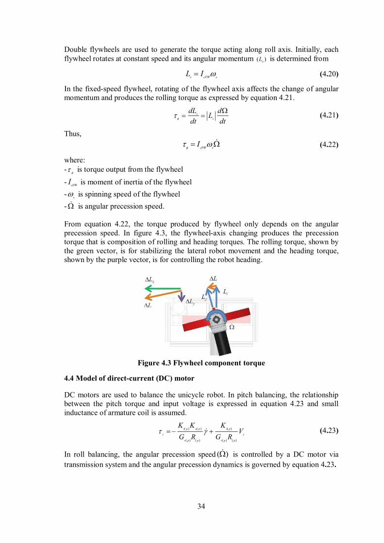
-  is angular precession speed.  From  equation  4.22,  the  torque  produced  by  flywheel  only  depends  on  the  angular precession  speed.  In  figure  4.3,  the  flywheel-axis  changing  produces  the  precession torque that is composition of rolling and heading torques. The rolling torque, shown by the green vector,  is  for  stabilizing  the  lateral  robot movement and  the heading  torque, shown by the purple vector, is for controlling the robot heading.  

 Figure 4.3 Flywheel component torque

4.4 Model of direct-current (DC) motor

DC motors are used to balance  the unicycle  robot.  In pitch balancing,  the  relationship between  the  pitch  torque  and  input  voltage  is  expressed  in  equation  4.23  and  small inductance of armature coil is assumed. 

 

   t p e p t p

r p p r p p

K K KV

G R G R

        (4.23)

In  roll  balancing,  the  angular  precession  speed ( )   is  controlled  by  a  DC  motor  via 

transmission system and the angular precession dynamics is governed by equation 4.23. 

 

35  

 

 t r e r t r

r r r r r r

K K KJ V

G R G R

       (4.24) 

When, 

- subscript  r shows roll axis, subscript  p shows pitch axis 

- is torque from driving wheel motor 

- is angular velocity of wheel motor  

-t

K is torque constant of the DC motor 

-e

K is back-emf (back-electromotive-force) constant 

-r

G is gear ratio 

- R is armature coil resistance - ,V V

is input voltage 

- J is moment of inertia of shaft with flywheel set 

 The dynamic  model of  the unicycle  robot can be expressed  in  the non-linear dynamic equation  as  shown  in  equation  4.25.  The  parameter  “M”  is  inertia  matrix.  “C”  is Coriolis matrix. “G”  is gravity matrix, and “D"  is disturbance matrix. The disturbance matrix  combines  the  equivalent  forces  from  external  disturbances,  frictions,  and parameter uncertainties. Coulomb friction  is also considered  in the disturbance matrix. Since the robot operates at low speed, the viscous friction is small and negligible. This term (D  matrix)  is separately  considered  from  the unicycle  robot dynamic  model. F  is the input force matrix.  

  ,  M q q C q q G q D F       (4.25) 

where: 

11 12 13 14 1

21 22 23 24 2

31 32 33 34 3

41 42 43 44 4

cFW

ratio

ratio

1

2

3

4

, ,     ,   0

e

e

s

t

t

M M M M C

M M M M CM C G D

M M M M C

M M M M C

i

KF V

RG

G

G

G

KK

G

K

VRG

 

1

2

3

4

-  sin( ) cos( ) sin( )

-  0

-  cos( )sin( )

-  0

F F w

F F

G m g r l gm r

G

G g l m

G

 

 

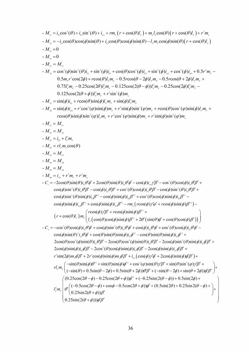
36  

2 2 2

11 F1 F3 w1

12 F1 F3

13

14

21 12

2 2

22 F1

-  cos ( ) sin ( ) cos( ) cos( ) cos( )

-  cos( )cos( )sin( ) cos( )cos( )sin( ) cos( )sin( ) cos( )

-   0

-   0

- 

-  cos ( )sin ( ) sin

F F F F F w

F F F

M i i i rm r l m l r l r m

M i i l m r l

M

M

M M

M i

2 2 2 2 2

F2 F3 w2 w3

2

2 2 2

( ) cos( )cos ( ) sin ( ) cos ( ) 0.5

            0.5 cos(2 ) cos( ) 0.5 cos( 2 ) 0.5 cos( 2 )

            0.75 0.25cos(2 ) 0.125cos(2( )) 0.25cos(2

F

F F F F F F F

F F F F F F

i i i i r m

m r r l m r l m r l m

l m l m l m

2

2 2 2

2

23 F2

2 2 2 2 2

24 w2

)

            0.125cos(2( )) sin ( )             

-  sin( ) cos( )sin( ) sin( )

-  sin( ) cos ( )sin( ) sin( )sin ( ) cos( )cos ( )sin( )

            

F F

F F w

F F F F

F F F F

l m

l m r m

M i r l m l m

M i r m r m r l m

r

2 2 2 2 2

31 13

32 23

2

33 F2

34

41 14

42

43

2 2

44 w

24

34

2

cos( )sin( )sin ( ) cos ( )sin( ) sin( )sin ( )

- 

- 

- 

-  cos( )

- 

- 

- 

- 

F F w w

F F

F F

F w

l m r m r m

M

M M

M M

M i l m

M rl m

M M

M

M

M i r m r m

M

 

2

1 F1 F3 w2 F1

2 2 2

F1 F2 F3 F3

2

-  2cos( )sin( ) 2cos( )sin( ) cos( ) cos ( )cos( )

          cos( )sin ( ) cos( ) cos ( )cos( ) cos( )sin ( )

          cos( )sin ( )sin( )

C i i i i

i i i i

i

2 2 2 2

F1 F2 F3

2 2 2

w2 w3

2

cos( )sin( ) cos ( )cos( )sin( )

          cos( )sin( ) cos( )sin( ) cos( ) cos( )sin( )

cos( ) cos( )sin( )           cos( )

cos( )cos( )sin(

w

F F

F

i i

i i rm r r

r rr l m

l

2

2 2 2

2 F1 F1 F2 F3

2 2

F3 F1 F3

) 2 sin( ) cos( )cos( )

-  cos ( )cos( ) cos( )sin ( ) cos( ) cos ( )cos( )

          cos( )sin( ) cos( )sin( )sin( ) cos( )sin( )sin( )

C i i i i

i i i

2

2 2 2

F1 F3 F1

2

F2 F3 w3

2

          2cos( )cos ( )sin( ) 2cos( )cos ( )sin( ) 2cos( )sin ( )sin( )

          2cos( )sin( ) 2cos ( )cos( )sin( ) 2cos( )sin( )

           sin(2 )F

i i i

i i i

r m

2

w2

2 2 2 2

2 cos( )sin( ) cos( ) 2cos( )sin( )

sin( )sin( ) sin( )sin( ) cos ( )sin( ) sin( )sin ( )          

( sin( ) 0.5sin( 2 ) 0.5sin( 2 )) ( sin( 2 ) sin(

w

F F

r m i

rl m

2

2

2 ))

(0.25cos(2 ) 0.25cos(2 )) ( 0.25sin(2( )) 0.5sin(2 )

( 0.5cos(2 ) cos 0.5cos(2 )) (0.5sin(2 ) 0.25sin2( )          

0.25sin2( ))

0.25sin(2( )))

F Fl m

     

 

 

37  

2 2

3 F3 F2 F3

ratio

2 2 2

F3 F3

2 2 2

F12

-  cos( )sin( ) cos( ) cos ( )cos( )

        cos( )sin ( ) cos( )cos ( )sin( )

cos( )sin( ) cos( ) cos ( ) sin ( )        

cos( )cos ( )sin(

e tK KC i i i

RG

i i

i

2

2

2 2 2 2 2

2

2

)

sin( ) sin( )sin( ) 2 cos( )cos( )        

0.5 sin( ) 0.5 cos ( )sin( ) 0.5 sin( )sin ( )

0.5sin(2 ) (0.5cos(2 ) cos( )

0.5cos(2 ))        

F F

F F

r r rl m

r r r

l m

2

2 24 w2

ratio

2

2

( 0.25sin(2 ) 0.125sin(2( ))

0.125sin(2( )))

-  cos( ) 2 cos( ) 2 cos( )

sin( ) 2sin( )sin( ) 2cos( )cos( )         

cos (

e tF w

F F

K KC i r m r m

RG

rl m

2 2 2)sin( ) sin( )sin ( )

 

 

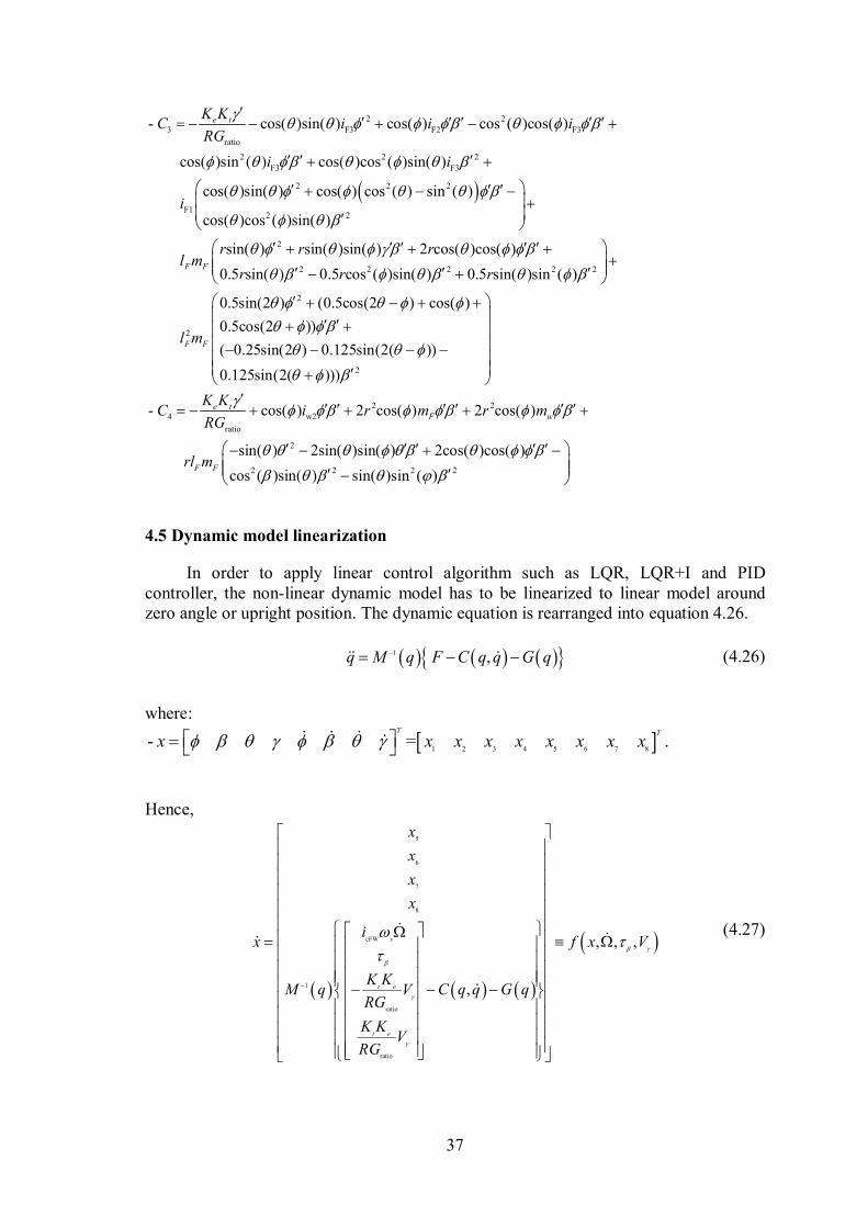
4.5 Dynamic model linearization

In  order  to  apply  linear  control  algorithm  such  as  LQR,  LQR+I  and  PID controller,  the  non-linear  dynamic  model  has  to  be  linearized  to  linear  model  around zero angle or upright position. The dynamic equation is rearranged into equation 4.26.  

  1   ,q M q F C q q G q       (4.26) 

 where: 

1 2 3 4 5 6 7 8-  = .

T T

x x x x x x x x x

   Hence, 

 

cFW

1

ratio

ratio

5

6

7

8

, ,

  ,

,s

t e

t e

ix f x V

K KM q C q q G qV

RG

K

x

K

G

x

VR

x

x

    (4.27) 

 

 

38  

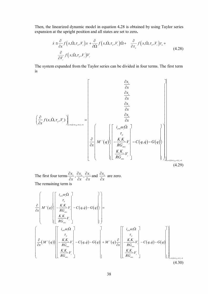
Then, the linearized dynamic model in equation 4.28 is obtained by using Taylor series expansion at the upright position and all states are set to zero.  

 

     , ,      , ,     , ,

      , ,

, , ,

,

x f x V x f x V f x Vx

f x V VV

  (4.28) 

The system expanded from the Taylor series can be divided in four terms. The first term is   

5

6

7

8

0, , 0

cFW

1

ratio

r

0

atio

0,

( , , ),  

  ,

x V

s

t e

t e

x

x

x

x

x

x

x

f x V xx

i

K KM q C q q G qV

x RG

K KV

RG

0 00,,0,x V

 

  (4.29) 

The first four terms 5x

x

, 6

x

x

, 7

x

x

and  8

x

x

 are zero. 

The remaining term is   

cFW

1

ratio

ratio

cFW

1

ratio

ratio

  ,

  ,

s

t e

t e

s

t e

t e

i

K KM q C q q G qV

x RG

K KV

RG

i

K KM q C q q G qV

x RG

K KV

RG

cFW

1

ratio

rati0 ,

o, , 000

,  

s

t e

t e

x V

i

K KM q C q q G qV

x RG

K KV

RG

 

  (4.30) 

 

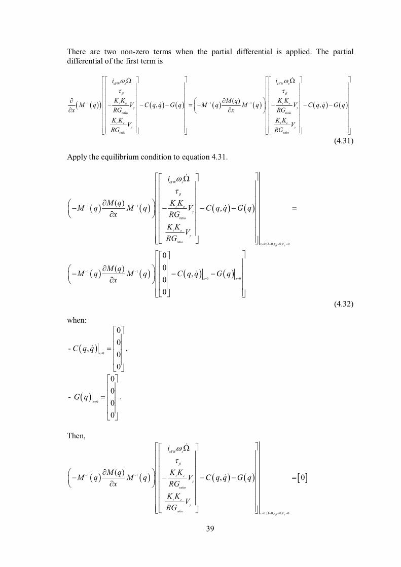
39  

There  are  two  non-zero  terms  when  the  partial  differential  is  applied.  The  partial differential of the first term is  

cFW cFW

1 1 1

ratio ratio

ratio ratio

( )  ,   ,

s s

t e t e

t e t e

i i

K K K KM qM q C q q G q M q M q C q q G qV V

x xRG RG

K K K KV V

RG RG

 

  (4.31) 

Apply the equilibrium condition to equation 4.31.   

cFW

1 1

ratio

ratio0, , 0

1

0

1

0 ,

0 0

( )  ,

0

( ),

0

0

0

s

t e

t e

x V

x x

i

M q K KM q M q C q q G qV

x RG

K KV

RG

M qM q M q C q q G q

x

 

  (4.32) 

when: 

0

0

0-  ,

0

0

xC q q

, 

0

0

0- 

0

0

xG q

.     

 Then, 

cFW

1 1

ratio

ratio0 , , 00 0,

( )  , 0

s

t e

t e

x V

i

M q K KM q M q C q q G qV

x RG

K KV

RG

 

 

40  

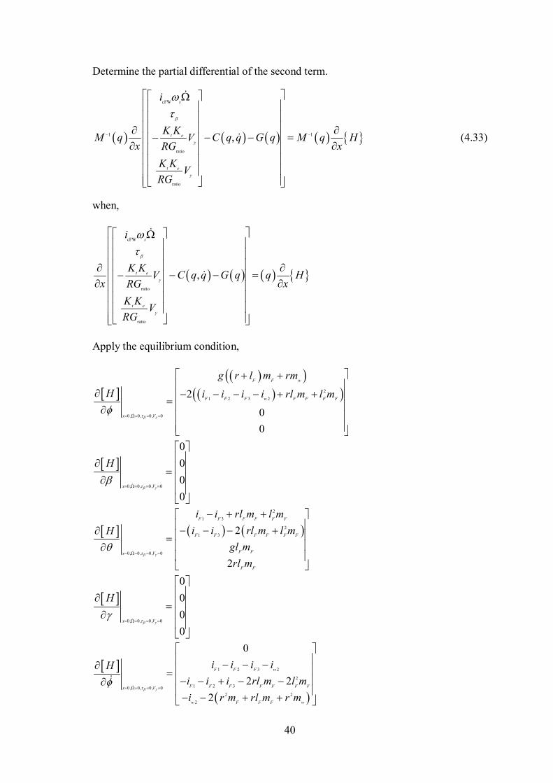
Determine the partial differential of the second term. 

cFW

1 1

ratio

ratio

,

s

t e

t e

i

K KM q C q q G q M q HV

x xRG

K KV

RG

      (4.33) 

when,   

cFW

ratio

ratio

,

s

t e

t e

i

K KC q q G q q HV

x xRG

K KV

RG

 

 Apply the equilibrium condition,  

2

1 2 3 2

0 , 00 ,,0

2

0

0

F F w

F F F w F F F F

x V

g r l m rm

H i i i i rl m l m

 

0, 0 ,,0 0

0

0

0

0x V

H

 

2

1 3

2

1 3

00, 00 ,,

2

2

F F F F F F

F F F F F F

F Fx V

F F

i i rl m l m

i i rl m l mH

gl m

rl m

 

0, 0 ,,0 0

0

0

0

0x V

H

 

1 2 3 2

2

1 2 30 , , 0

2

0

2

,

2

0

0

2 2

2

F F F w

F F F F F F Fx V

w F F F w

i i i iH

i i i rl m l m

i r m rl m r m

 

 

41  

1 2 3 2

2

1 2 30 , , 0

2

0

2

2

0 ,

0

2 2

2

F F F w

F F F F F F Fx V

w F F F w

i i i i

H

i i i rl m l m

i r m rl m r m

 

2

2 1 3

2

0 0,

2 1 3

0 , , 0

2

0

0

F F F F F F F

F F F F F

x V

i rl m l m i i

H i i i l m

 

0

2 2

2

ratio0 , , 0 , 0

ratio

0

w F F F w

e t

x V

e t

i r m rl m r m

H K K

RG

K K

RG

 

Finally, 

cFW

1

ratio

ratio

1 7 3 4 2 3 7 2 6

2

2 3 7 4 2 7

1

5 5

ratio

2 6 2 6

,

0 0 0 2

0 2 0 0 0

0 0 0 0*

0 0 2 0 2 2

s

t e

t e

F w

F F F

e t

F F

F F w w

i

K KM q C q q G qV

x RG

K KV

RG

i i

i l m

K Kgl mM

RG

rl m i i

ratio

0 e tK K

RG

(4.34) 

 When: 

1

2

2 4

2

3

4 1 2 3 2

2

5 1 2 3

2 2

6

7 1 3

- 

-  2

- 

- 

-  2 2

- 

- 

F F w

F F F F

F F F F

F F F w

F F F F F F F

F F F w

F F

g r l m rm

rl m l m

rl m l m

i i i i

i i i rl m l m

r m rl m r m

i i

 

*M is the symmetrical positive definite matrix of  the  robot  inertia and evaluated at  the 

upright position.

 

42  

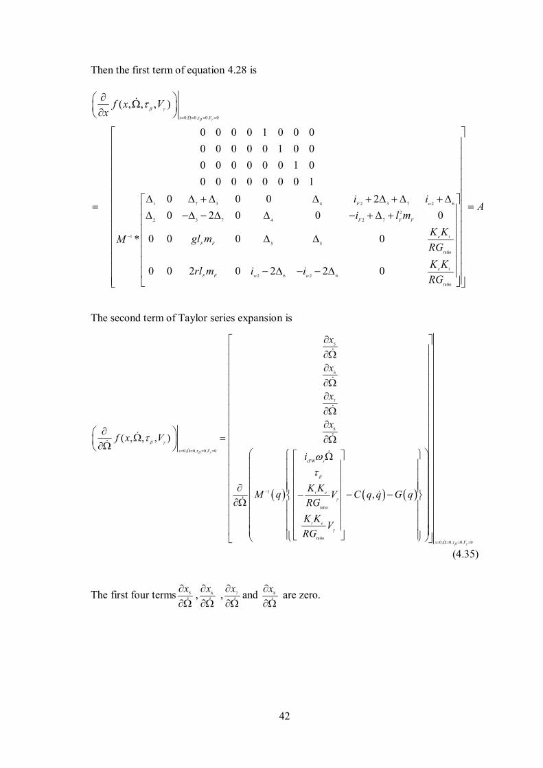
Then the first term of equation 4.28 is   

0, , 0

1 7 3 4

0

2 3 7 2 6

2

2 3 7 4 2 7

1

5 5

0 ,

ratio

( , , )  

0 0 0 0 1 0 0 0

0 0 0 0 0 1 0 0                              

0 0 0 0 0 0 1 0

0 0 0 0 0 0 0 1

0 0 0 2   

0 2 0 0 0

0 0 0 0*

0 0 2 0

,x V

F w

F F F

e t

F F

F F

f x Vx

i i

i l m

K Kgl mM

RG

rl m

2 6 2 6

ratio

2 2 0 e t

w w

A

K Ki i

RG

 

The second term of Taylor series expansion is 

5

6

7

8

0, , 0

cFW

1

ra

0 0,

tio

ratio

( , , )  

  ,

,x V

s

t e

t e

x

x

x

x

f x V

i

K KM q C q q G qV

RG

K KV

RG

0, 0 0, 0,x V

 

  (4.35) 

 

The first four terms 5x

, 6

x

 , 7

x

and  8

x

 are zero. 

   

 

43  

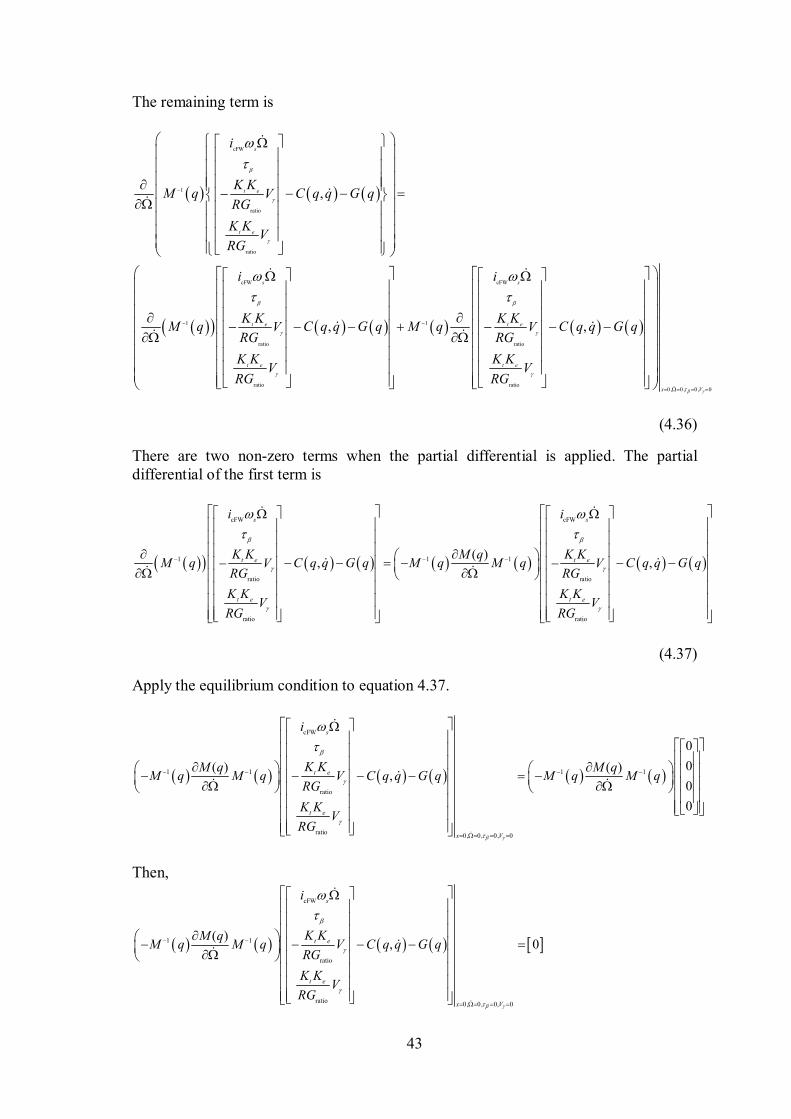
The remaining term is   

cFW

1

ratio

ratio

cFW

1

ratio

ratio

  ,

  ,

s

t e

t e

s

t e

t e

i

K KM q C q q G qV

RG

K KV

RG

i

K KM q C q q G qV

RG

K KV

RG

0 0

cFW

1

ratio

rati,

o0 , , 0

,  

s

t e

t e

x V

i

K KM q C q q G qV

RG

K KV

RG

   (4.36) 

There  are  two  non-zero  terms  when  the  partial  differential  is  applied.  The  partial differential of the first term is  

cFW cFW

1 1 1

ratio ratio

ratio ratio

( )  ,   ,

s s

t e t e

t e t e

i i

K K K KM qM q C q q G q M q M q C q q G qV V

RG RG

K K K KV V

RG RG

   (4.37) 

Apply the equilibrium condition to equation 4.37.  

cFW

1 1 1 1

ratio

ratio0, 0 0,, 0

0

( ) ( )  ,

0

0

0

s

t e

t e

x V

i

K KM q M qM q M q C q q G q M q M qV

RG

K KV

RG

 Then, 

cFW

1 1

ratio

ratio0, 00 0,,

( )  , 0

s

t e

t e

x V

i

K KM qM q M q C q q G qV

RG

K KV

RG

 

 

44  

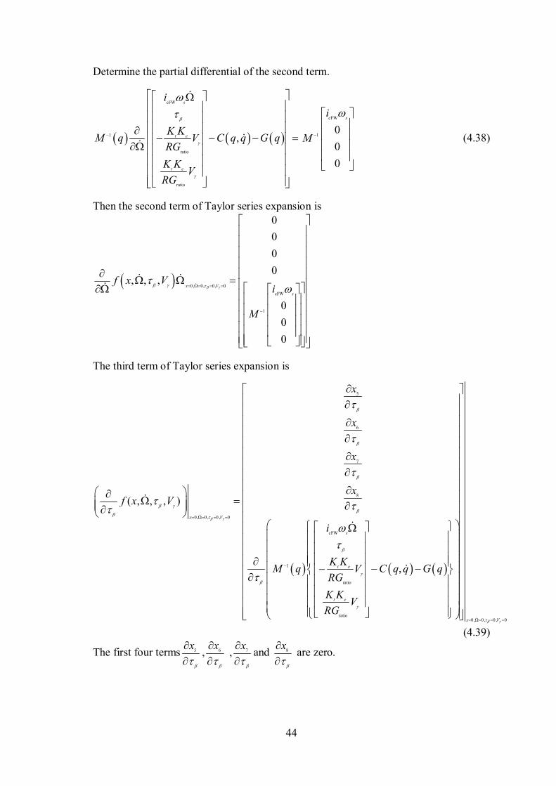
Determine the partial differential of the second term. 

cFW

1

ratio

ratio

,

s

t e

t e

i

K KM q C q q G qV

RG

K KV

RG

cFW

1

0

0

0s

i

M

        (4.38) 

Then the second term of Taylor series expansion is  

0 0,0 , , 0

cFW

1

,

0

0

0

0, ,

0

0

0

x V

s

f x Vi

M

 

The third term of Taylor series expansion is 

5

6

7

8

0, , 0

cFW

1

rat

0 0

io

ratio

,

( , ,  

 

, )

,

x V

s

t e

t e

x

x

x

xf x V

i

K KM q C q q G qV

RG

K KV

RG

0 , 0 0 ,, 0x V

  (4.39) 

The first four terms 5x

, 6

x

 , 7

x

and  8

x

 are zero. 

   

 

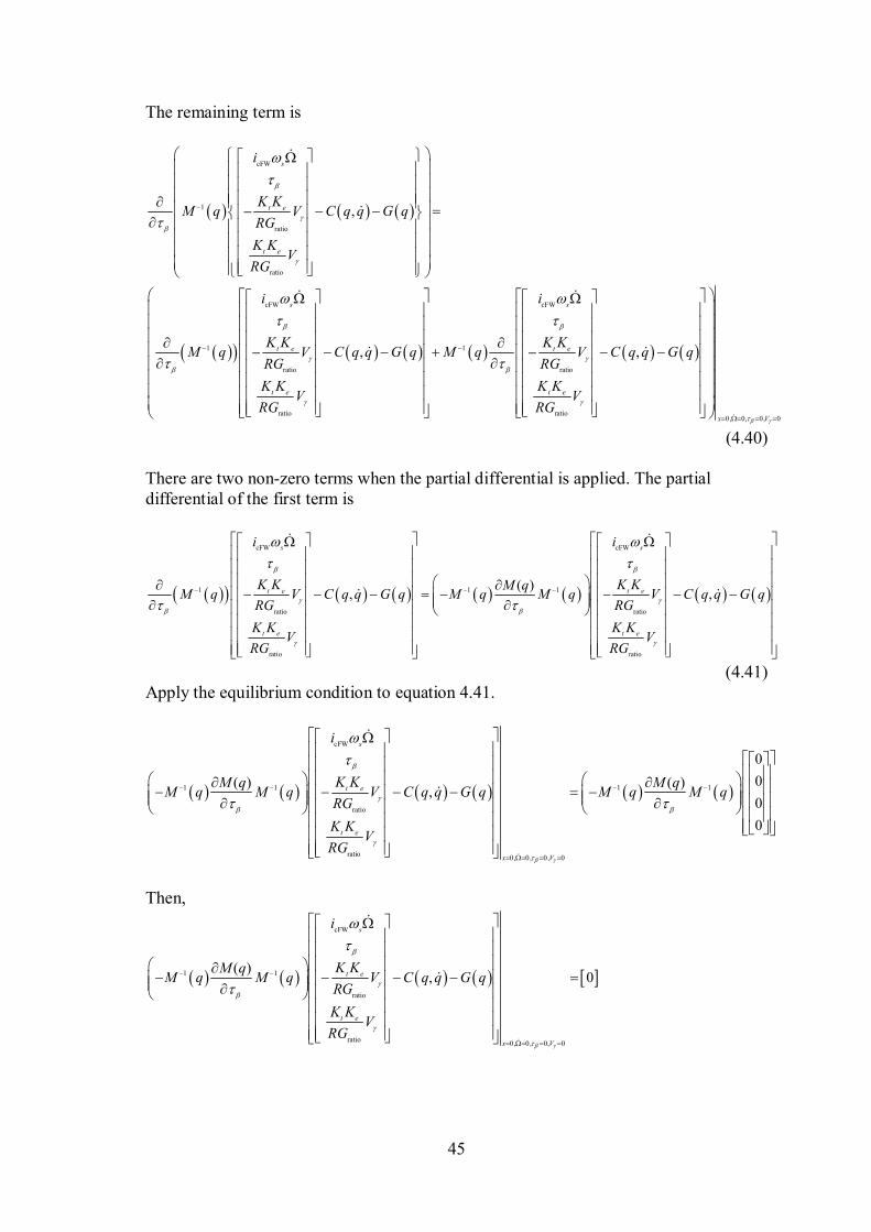
45  

The remaining term is   

cFW

1

ratio

ratio

cFW

1

ratio

ratio

  ,

  ,

s

t e

t e

s

t e

t e

i

K KM q C q q G qV

RG

K KV

RG

i

K KM q C q q G qV

RG

K KV

RG

cFW

1

ratio

ratio0, 0,,0 0

,  

s

t e

t e

x V

i

K KM q C q q G qV

RG

K KV

RG

  (4.40)  

There are two non-zero terms when the partial differential is applied. The partial differential of the first term is  

cFW cFW

1 1 1

ratio ratio

ratio ratio

( )  ,   ,

s s

t e t e

t e t e

i i

K K K KM qM q C q q G q M q M q C q q G qV V

RG RG

K K K KV V

RG RG

(4.41) Apply the equilibrium condition to equation 4.41.  

cFW

1 1 1 1

ratio

ratio0, 0 0, 0,

0

( ) ( ) 

0

0

0,

s

t e

t e

x V

i

K KM q M qM q M q C q q G q M q M qV

RG

K KV

RG

 Then, 

cFW

1 1

ratio

ratio0, ,0 00,

( )  , 0

s

t e

t e

x V

i

K KM qM q M q C q q G qV

RG

K KV

RG

 

   

 

46  

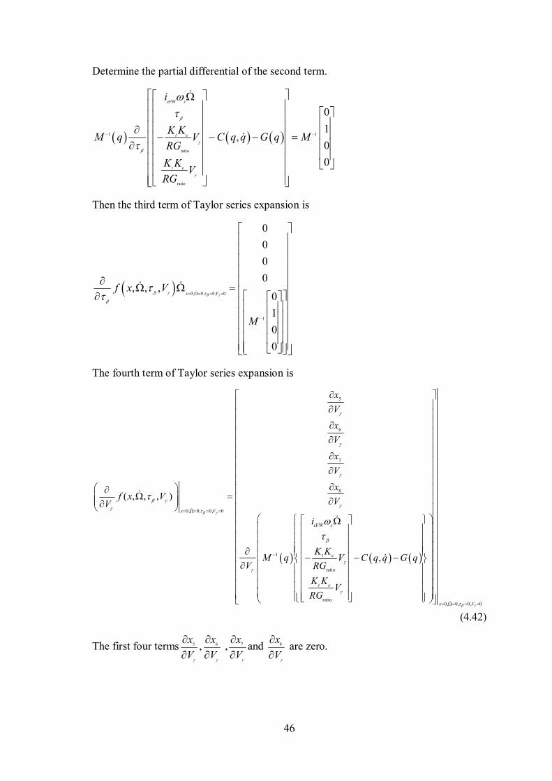
Determine the partial differential of the second term. 

cFW

1 1

ratio

ratio

1

0

,0

0

s

t e

t e

i

K KM q C q q G q MV

RG

K KV

RG

 

Then the third term of Taylor series expansion is  

0 00, ,

1

, 0

0

0

0

0, ,

0,

1

0

0

x Vf x V

M

 

The fourth term of Taylor series expansion is 

5

6

7

8

0, , 0

cFW

1

r

0

atio

rat

0

io

,

( , , )  

  ,

,

x V

s

t e

t e

x

V

x

V

x

V

xf x V

VV

i

K KM q C q q G qV

V RG

K KV

RG

0 0,0, , 0x V

 

  (4.42) 

The first four terms 5x

V

, 6

x

V

 , 7

x

V

and  8

x

V

 are zero. 

   

 

47  

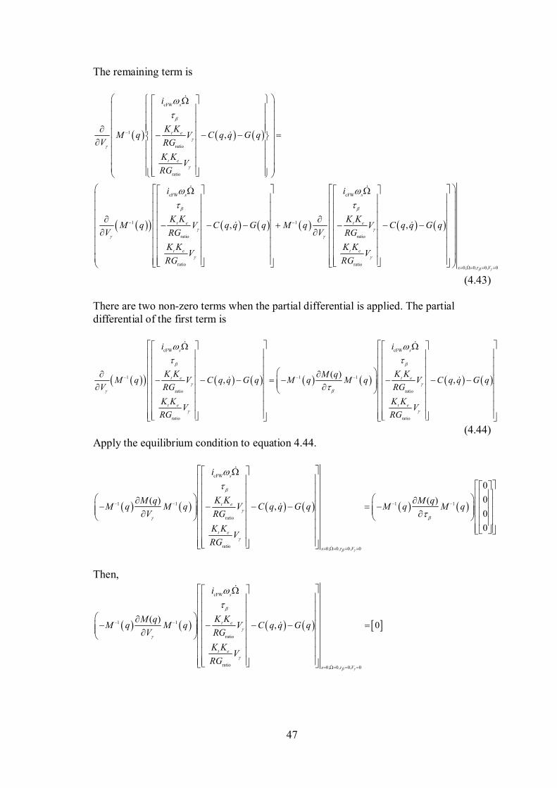
The remaining term is   

cFW

1

ratio

ratio

cFW

1

ratio

ratio

  ,

  ,

s

t e

t e

s

t e

t e

i

K KM q C q q G qV

V RG

K KV

RG

i

K KM q C q q G qV

V RG

K KV

RG

cFW

1

ratio

ratio0, , 00 0,

,  

s

t e

t e

x V

i

K KM q C q q G qV

V RG

K KV

RG

  (4.43)  

There are two non-zero terms when the partial differential is applied. The partial differential of the first term is  

cFW cFW

1 1 1

ratio ratio

ratio ratio

( )  ,   ,

s s

t e t e

t e t e

i i

K K K KM qM q C q q G q M q M q C q q G qV V

V RG RG

K K K KV V

RG RG

  (4.44) Apply the equilibrium condition to equation 4.44.    

cFW

1 1 1 1

ratio

ratio0, 0 0, 0,

0

( ) ( ) 

0

0

0,

s

t e

t e

x V

i

K KM q M qM q M q C q q G q M q M qV

V RG

K KV

RG

 Then, 

cFW

1 1

ratio

ratio0, , 00 0,

( )  , 0

s

t e

t e

x V

i

K KM qM q M q C q q G qV

V RG

K KV

RG

 

   

 

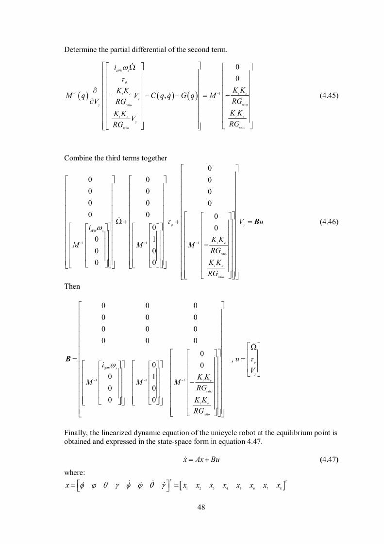
48  

Determine the partial differential of the second term. 

cFW

1 1

ratioratio

ratioratio

0

0

,

s

t et e

t et e

i

K KK KM q C q q G q MV

RGV RG

K KK KV

RGRG

      (4.45) 

 

Combine the third terms together  

cFW

1 1 1

ratio

ratio

0

0 0 0

0 0 0

0 0 0

0 0

0

0

0

0

1

0 0

0 0

s

t e

t e

i

K KM M M

RG

K K

RG

V u

B       (4.46) 

Then   

cFW

1 1 1

ratio

ratio

0 0 0

0 0 0

0 0 0

0 0 0

0   , 

0

1

0

0 0

0

0

0

s

t e

t e

ui

VK K

M M MRG

K K

RG

B

 

 Finally, the linearized dynamic equation of the unicycle robot at the equilibrium point is obtained and expressed in the state-space form in equation 4.47.    x Ax Bu            (4.47) 

where: 

1 2 3 4 5 6 7 8

T T

x x x x x x x x x  

 

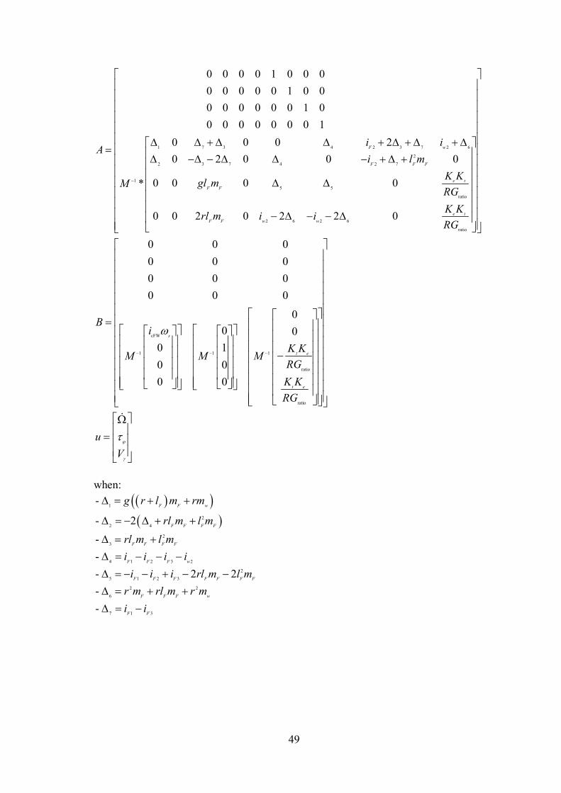
49  

1 7 3 4 2 3 7 2 6

2

2 3 7 4 2 7

1

5 5

ratio

2 6 2 6

ratio

0 0 0 0 1 0 0 0

0 0 0 0 0 1 0 0                              

0 0 0 0 0 0 1 0

0 0 0 0 0 0 0 1

0 0 0 2

0 2 0 0 0

0 0 0 0*

0 0 2 0 2 2 0

F w

F F F

e t

F F

e t

F F w w

i iA

i l m

K Kgl mM

RG

K Krl m i i

RG

 

cFW

1 1 1

ratio

ratio

0 0 0

0 0 0

0 0 0

0 0 0

0

0

0 1

0 0

0 0

0s

t e

t e

Bi

K KM M M

RG

K K

RG

 

u

V

 

 when: 

1

2

2 4

2

3

4 1 2 3 2

2

5 1 2 3

2 2

6

7 1 3

- 

-  2

- 

- 

-  2 2

- 

- 

F F w

F F F F

F F F F

F F F w

F F F F F F F

F F F w

F F

g r l m rm

rl m l m

rl m l m

i i i i

i i i rl m l m

r m rl m r m

i i

 

   

 

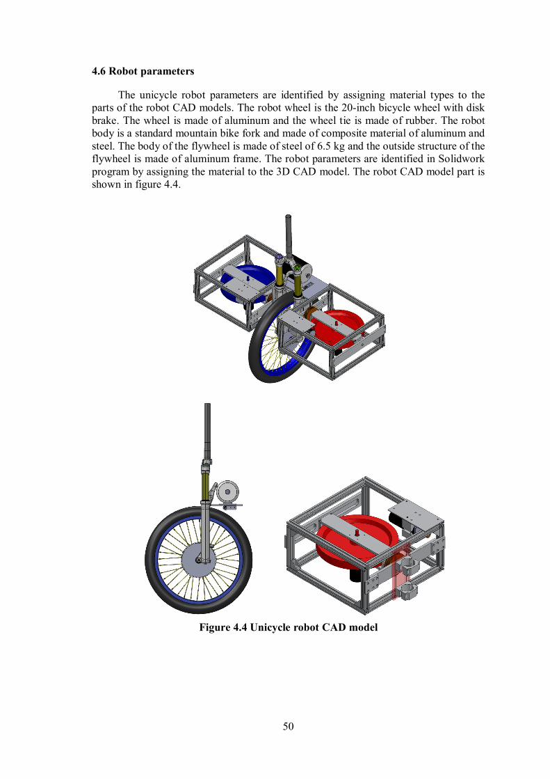
50  

4.6 Robot parameters

The  unicycle  robot  parameters  are  identified  by  assigning  material  types  to  the parts of the robot CAD models. The robot wheel is the 20-inch bicycle wheel with disk brake. The wheel  is made of aluminum and the wheel tie is made of rubber. The robot body is a standard mountain bike fork and made of composite material of aluminum and steel. The body of the flywheel is made of steel of 6.5 kg and the outside structure of the flywheel is made of aluminum frame. The robot parameters are identified in Solidwork program by assigning the material to the 3D CAD model. The robot CAD model part is shown in figure 4.4.  

 

 Figure 4.4 Unicycle robot CAD model

    

 

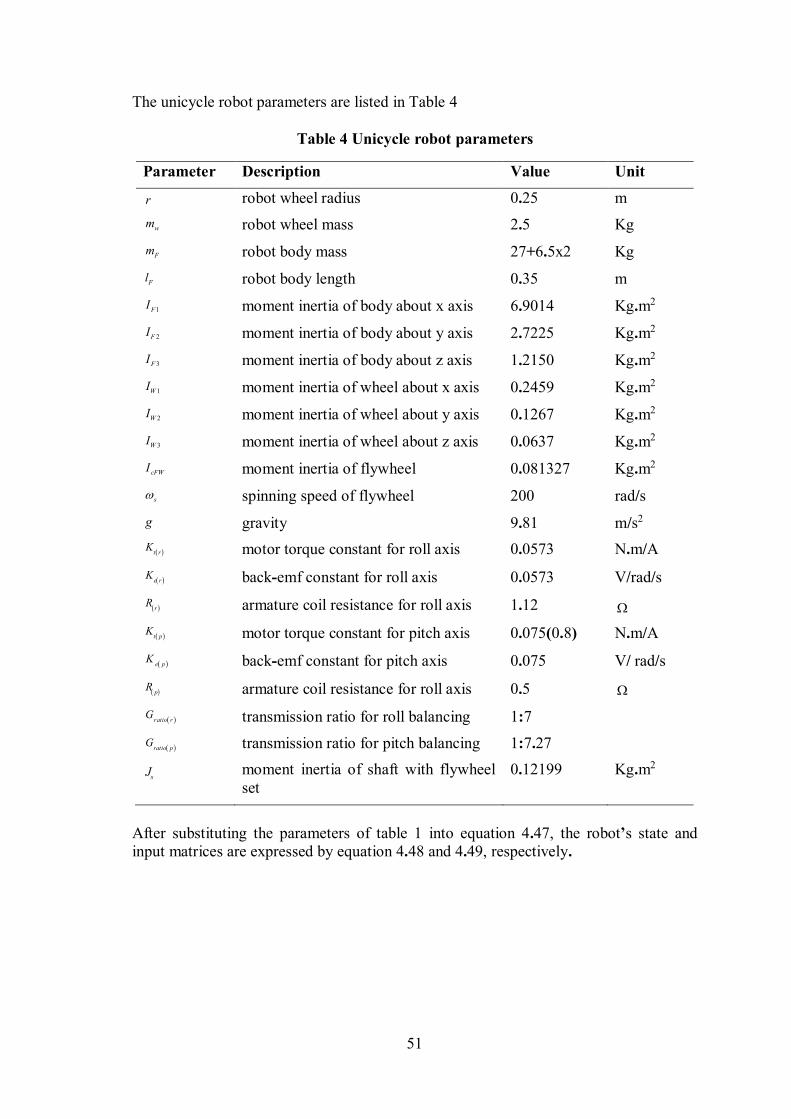
51  

The unicycle robot parameters are listed in Table 4   Table 4 Unicycle robot parameters

Parameter Description Value Unit

r   robot wheel radius  0.25  m 

wm   robot wheel mass  2.5  Kg 

Fm   robot body mass   27+6.5x2  Kg 

Fl   robot body length  0.35  m 

1FI   moment inertia of body about x axis  6.9014  Kg.m2 

2FI   moment inertia of body about y axis  2.7225  Kg.m2 

3FI   moment inertia of body about z axis  1.2150  Kg.m2 

1WI   moment inertia of wheel about x axis  0.2459  Kg.m2 

2WI   moment inertia of wheel about y axis  0.1267  Kg.m2 

3WI   moment inertia of wheel about z axis  0.0637  Kg.m2 

cFWI   moment inertia of flywheel   0.081327  Kg.m2 

s   spinning speed of flywheel  200  rad/s 

g   gravity  9.81  m/s2 

t rK   motor torque constant for roll axis  0.0573  N.m/A 

e rK   back-emf constant for roll axis  0.0573  V/rad/s 

rR   armature coil resistance for roll axis  1.12   

t pK   motor torque constant for pitch axis  0.075(0.8)  N.m/A 

e pK   back-emf constant for pitch axis  0.075  V/ rad/s 

pR   armature coil resistance for roll axis  0.5   

ratio rG  

ratio pG  

sJ  

transmission ratio for roll balancing 

transmission ratio for pitch balancing 

moment  inertia  of  shaft  with  flywheel set 

1:7 

1:7.27 

0.12199 

 

 

Kg.m2 

 After  substituting  the  parameters  of  table  1  into  equation  4.47,  the  robot’s  state  and input matrices are expressed by equation 4.48 and 4.49, respectively. 

 

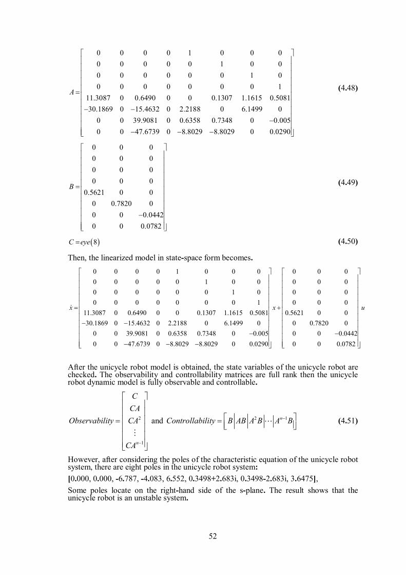
52  

0 0 0 0 1 0 0 0

0 0 0 0 0 1 0 0

0 0 0 0 0 0 1 0

0 0 0 0 0 0 0 1

11.3087 0 0.6490 0 0 0.1307 1.1615 0.5081

30.1869 0 15.4632 0 2.2188 0 6.1499 0

0 0 39.9081 0 0.6358 0.7348 0 0.005

0 0 47.6739 0 8.8029 8.8029 0 0.0290

 A

    (4.48)

0 0 0

0 0 0

0 0 0

0 0 0

0.5621 0 0

0 0.7820 0

0 0 0.0442

0 0 0.0782

 B

              (4.49) 

  8C eye                     (4.50) 

Then, the linearized model in state-space form becomes.  

0 0 0 0 1 0 0 0 0 0 0

0 0 0 0 0 1 0 0 0 0 0

0 0 0 0 0 0 1 0 0 0 0

0 0 0 0 0 0 0 1

11.3087 0 0.6490 0 0 0.1307 1.1615 0.5081

30.1869 0 15.4632 0 2.2188 0 6.1499 0

0 0 39.9081 0 0.6358 0.7348 0 0.005

0 0 47.6739 0 8.8029 8.8029 0 0.0

 

290

xx

0 0 0

0.5621 0 0

0 0.7820 0

0 0 0.0442

0 0 0.0782

u

 

After the unicycle robot model is obtained, the state variables of the unicycle robot are checked. The observability  and controllability  matrices are  full  rank  then  the unicycle robot dynamic model is fully observable and controllable.  

2

1n

C

CA

Observability CA

CA

and  2 1nControllability B AB A B A B

    (4.51)

However, after considering the poles of the characteristic equation of the unicycle robot system, there are eight poles in the unicycle robot system:  

[0.000, 0.000, -6.787, -4.083, 6.552, 0.3498+2.683i, 0.3498-2.683i, 3.6475],  

Some  poles  locate  on  the  right-hand  side  of  the  s-plane. The  result  shows  that  the unicycle robot is an unstable system. 

   

 

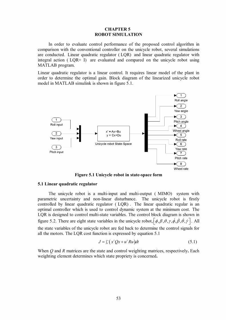
53  

CHAPTER 5 ROBOT SIMULATION

In  order  to  evaluate  control  performance  of  the  proposed  control  algorithm  in comparison  with  the  conventional  controller  on  the  unicycle  robot,  several  simulations are  conducted.   Linear  quadratic  regulator  ( LQR)   and  linear  quadratic  regulator  with integral  action  ( LQR+ I)   are  evaluated  and  compared  on  the  unicycle  robot  using MATLAB program.   

Linear  quadratic  regulator  is  a  linear  control.  It  requires  linear  model  of  the  plant  in order  to  determine  the  optimal  gain.  Block  diagram  of  the  linearized  unicycle  robot model in MATLAB simulink is shown in figure 5.1.

 

Figure 5.1 Unicycle robot in state-space form

5.1 Linear quadratic regulator

The  unicycle  robot  is  a  multi-input  and  multi-output  ( MIMO)   system  with parametric  uncertainty  and  non-linear  disturbance.   The  unicycle  robot  is  firstly controlled  by  linear  quadratic  regulator  ( LQR) .   The  linear  quadratic  regular  is  an optimal controller  which  is  used  to  control  dynamic  system  at  the  minimum  cost.   The LQR is designed to control multi-state variables. The control block diagram is shown in 

figure 5.2. There are eight state variables in the unicycle robot, , , , , , , , . All 

the state variables of the unicycle robot are fed back to determine the control signals for all the motors. The LQR cost function is expressed by equation 5.1 

  0

T TJ x Qx u Ru dt

        (5.1) 

When Q and R matrices are the state and control weighting matrices, respectively. Each weighting element determines which state propriety is concerned.  

 

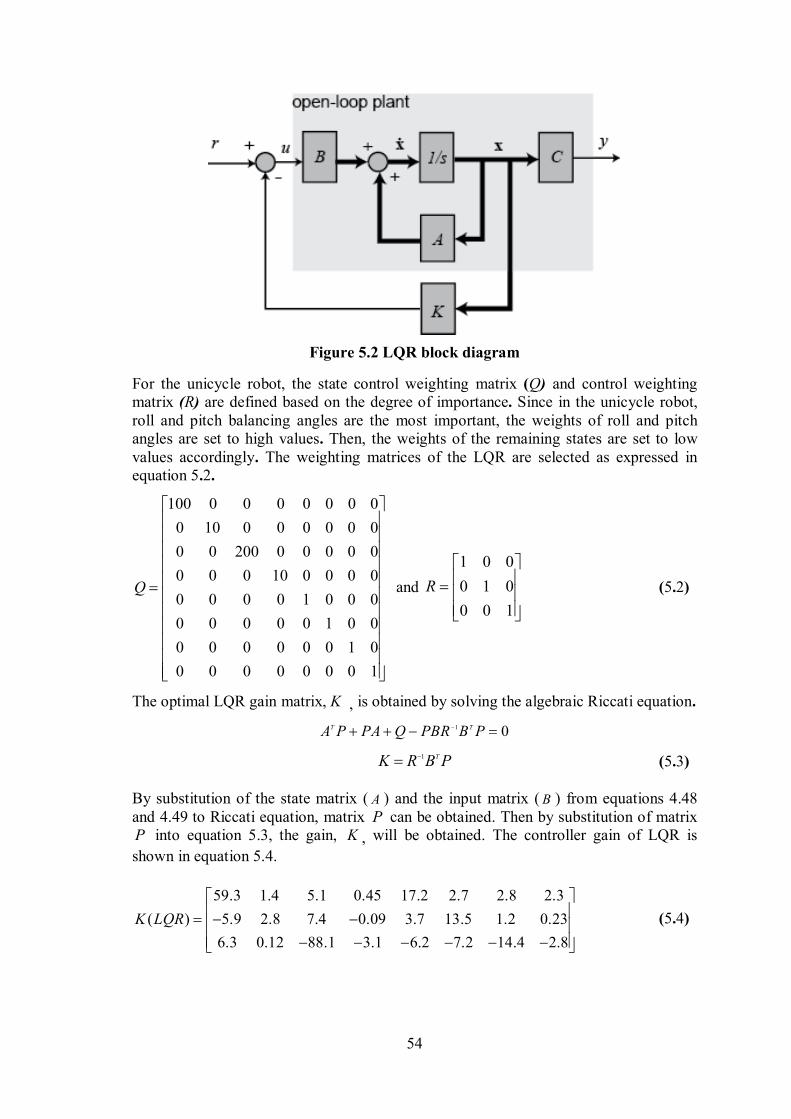
54  

Figure 5.2 LQR block diagram 

For  the  unicycle  robot,  the  state  control  weighting  matrix  (Q)  and  control  weighting matrix (R) are defined based on the degree of  importance. Since  in the unicycle robot, roll  and  pitch  balancing  angles  are  the  most  important,  the  weights  of  roll  and  pitch angles are  set  to high  values. Then,  the weights of  the  remaining states are  set  to  low values  accordingly. The  weighting  matrices  of  the  LQR  are  selected  as  expressed  in equation 5.2. 

100 0 0 0 0 0 0 0

0 10 0 0 0 0 0 0

0 0 200 0 0 0 0 0

0 0 0 10 0 0 0 0

0 0 0 0 1 0 0 0

0 0 0 0 0 1 0 0

0 0 0 0 0 0 1 0

0 0 0 0 0 0 0 1

Q

  and 

1 0 0

0 1 0

0 0 1

R

      (5.2)

The optimal LQR gain matrix, K , is obtained by solving the algebraic Riccati equation.

1 0T TA P PA Q PBR B P  

  1 TK R B P            (5.3) 

By substitution of  the state matrix  ( A )  and  the  input matrix  ( B )  from equations 4.48 and 4.49 to Riccati equation, matrix  P  can be obtained. Then by substitution of matrix P   into  equation  5.3,  the  gain,  K ,  will  be  obtained.  The  controller  gain  of  LQR  is 

shown in equation 5.4. 

59.3 1.4 5.1 0.45 17.2 2.7 2.8 2.3

( ) 5.9 2.8 7.4 0.09 3.7 13.5 1.2 0.23

6.3 0.12 88.1 3.1 6.2 7.2 14.4 2.8

K LQR

    (5.4) 

   

 

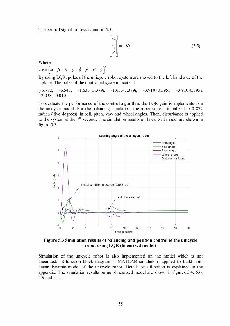
55  

The control signal follows equation 5.5, 

  Kx

V

           (5.5)

Where:  

- T

x  

By using LQR, poles of the unicycle robot system are moved to the left hand side of the s-plane. The poles of the controlled system locate at 

[-6.782,  -6.543,  -1.633+3.379i,  -1.633-3.379i,  -3.910+0.395i,  -3.910-0.395i,  -2.038, -0.010] 

To evaluate the performance of  the control algorithm, the LQR gain is implemented on the unicycle model.  For  the balancing simulation,  the  robot  state is  initialized  to 0.872 radian ( five degrees) in roll, pitch, yaw and wheel angles. Then, disturbance is applied to the system at the 7th second. The simulation results on linearized model are shown in figure 5.3.

Figure 5.3 Simulation results of balancing and position control of the unicycle robot using LQR (linearized model)

Simulation  of  the  unicycle  robot  is  also  implemented  on  the  model  which  is  not linearized.    S-function  block  diagram  in  MATLAB  simulink  is  applied  to  build  non-linear  dynamic  model  of  the  unicycle  robot.  Details  of  s-function  is  explained  in  the appendix. The simulation results on non-linearized model are shown in figures 5.4, 5.6, 5.9 and 5.11.  

 

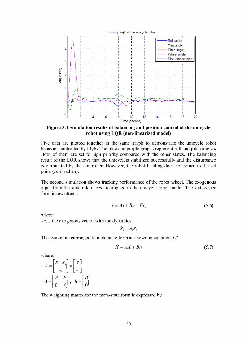
56  

Figure 5.4 Simulation results of balancing and position control of the unicycle

robot using LQR (non-linearized model) 

Five  data  are  plotted  together  in  the  same  graph  to  demonstrate  the  unicycle  robot behavior controlled by LQR. The blue and purple graphs represent roll and pitch angles. Both  of  them  are  set  to  high  priority  compared  with  the  other  states. The  balancing result of the LQR shows that the unicycleis stabilized successfully and the disturbance is  eliminated  by  the  controller. However,  the  robot  heading  does  not  return  to  the  set point (zero radian).  

The second simulation shows tracking performance of the robot wheel. The exogenous input from the state references are applied to the unicycle robot model. The state-space form is rewritten as  

 0

x Ax Bu Ex         (5.6) 

where:  

0- x is the exogenous vector with the dynamics  

0 0 0x A x  

The system is rearranged to meta-state form as shown in equation 5.7 

  X AX Bu           (5.7) 

where: 

0

0 0

0

- 

-  ,   0 0

x x eX

x x

A E BA B

A

 

The weighting martix for the meta-state form is expressed by  

 

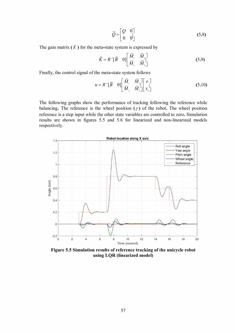
57  

 0

0 0

QQ

           (5.8) 

The gain matrix ( K ) for the meta-state system is expressed by  

  1 1 2

2 3

[ 0]M M

K R BM M

(5.9) 

Finally, the control signal of the meta-state system follows 

  1 1 2

02 3

[ 0]eM M

u R BxM M

       (5.10)

The  following graphs  show the performance of  tracking following  the  reference while balancing. The  reference  is  the  wheel  position  ( ) of  the  robot. The  wheel  position 

reference is a step input while the other state variables are controlled to zero. Simulation results  are shown  in  figures  5.5 and  5.6  for  linearized  and  non-linearized  models respectively. 

Figure 5.5 Simulation results of reference tracking of the unicycle robot

using LQR (linearized model)

 

 

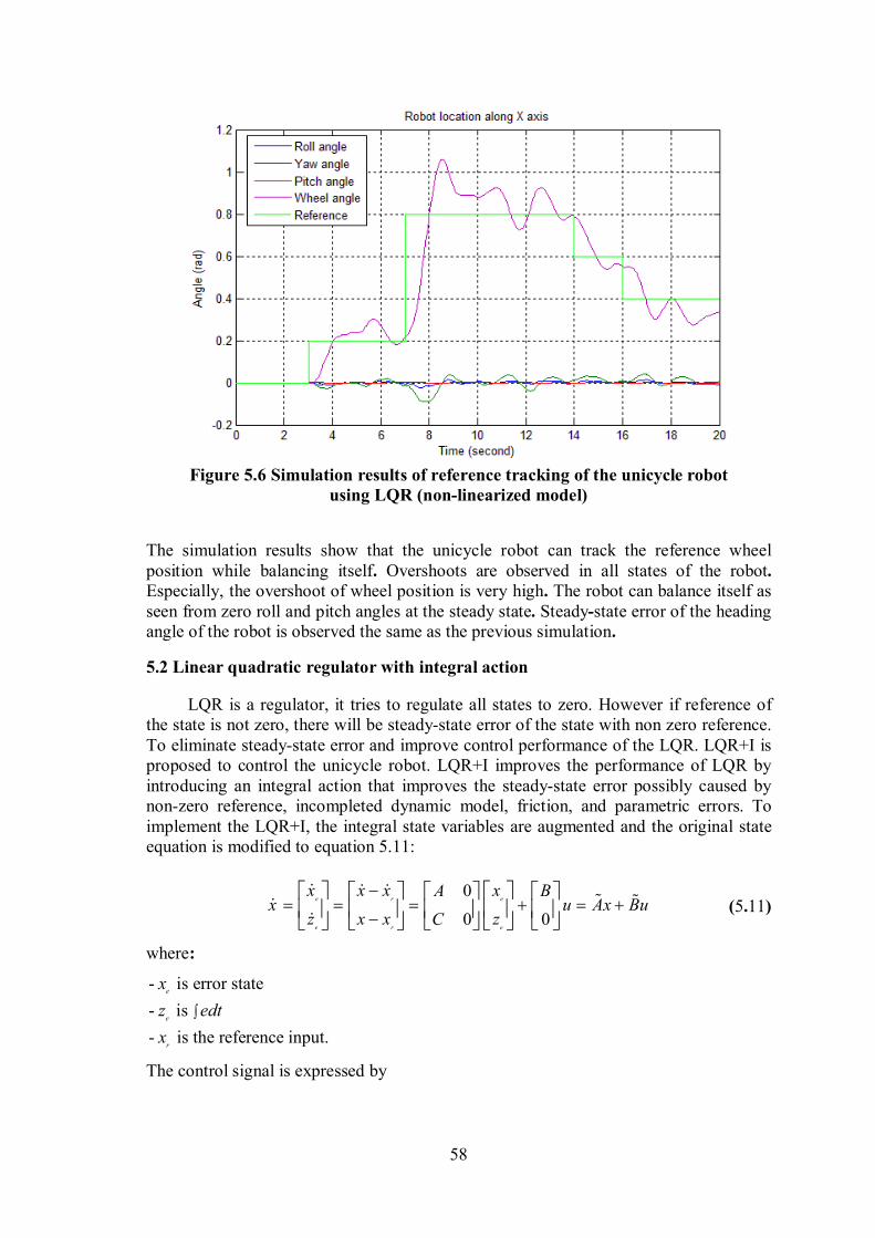
58  

 Figure 5.6 Simulation results of reference tracking of the unicycle robot

using LQR (non-linearized model)

 The  simulation  results  show  that  the  unicycle  robot  can  track  the  reference  wheel position  while  balancing  itself. Overshoots  are  observed  in  all  states  of  the  robot. Especially, the overshoot of wheel position is very high. The robot can balance itself as seen from zero roll and pitch angles at the steady state. Steady-state error of the heading angle of the robot is observed the same as the previous simulation. 

5.2 Linear quadratic regulator with integral action

LQR is a regulator,  it  tries to regulate all states  to zero. However  if reference of the state is not zero, there will be steady-state error of the state with non zero reference. To eliminate steady-state error and improve control performance of the LQR. LQR+I is proposed  to  control  the  unicycle  robot. LQR+I  improves  the  performance of  LQR by introducing  an  integral  action  that  improves  the  steady-state  error  possibly  caused  by non-zero  reference,  incompleted  dynamic  model,  friction,  and  parametric  errors.  To implement the LQR+I, the integral state variables are augmented and the original  state equation is modified to equation 5.11:  

 

 0

  0 0

e er

e er

x xx x A Bx u Ax Bu

z zx x C

    (5.11) 

where: 

-   is error state

-   is 

-   is the reference input.

e

e

r

x

z edt

x

The control signal is expressed by 

 

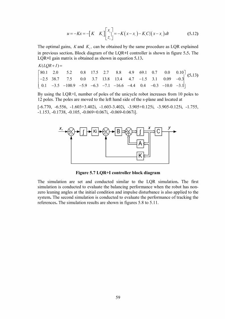
59  

  e

i r i r

e

xu Kx K K K x x K C x x dt

z

    (5.12) 

The optimal gains, K and  iK , can be obtained by the same procedure as LQR explained 

in previous section. Block diagram of the LQR+I controller is shown in figure 5.5. The LQR+I gain matrix is obtained as shown in equation 5.13. 

( )

80.1 2.0 5.2 0.8 17.5 2.7 8.8 4.9 69.1 0.7 0.0 0.10

2.5 38.7 7.5 0.0 3.7 13.8 13.4 4.7 1.5 3.1 0.09 0.3

0.1 3.5 100.9 5.9 6.3 7.1 16.6 4.4 0.4 0.3 10.0 3.1

K LQR I

 (5.13) 

By using the LQR+I, number of poles of the unicycle robot increases from 10 poles to 12 poles. The poles are moved to the left hand side of the s-plane and located at  

[-6.770,  -6.556,  -1.603+3.402i,  -1.603-3.402i,  -3.905+0.125i,  -3.905-0.125i,  -1.755,  -1.153, -0.1738, -0.105, -0.069+0.067i, -0.069-0.067i]. 

 

Figure 5.7 LQR+I controller block diagram

The  simulation  are  set  and  conducted  similar  to  the  LQR  simulation. The  first simulation is conducted to evaluate the balancing performance when the robot has non-zero leaning angles at the initial condition and impulse disturbance is also applied to the system. The second simulation is conducted to evaluate the performance of tracking the references. The simulation results are shown in figures 5.8 to 5.11. 

 

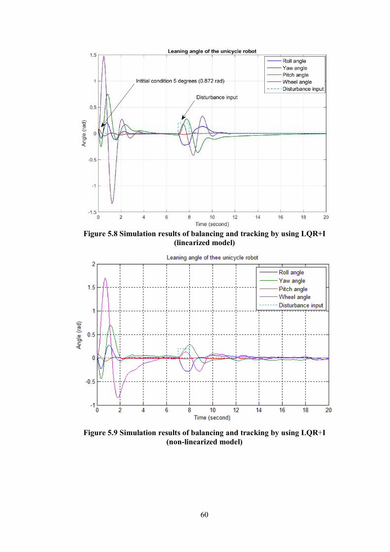
60  

 Figure 5.8 Simulation results of balancing and tracking by using LQR+I

(linearized model)

Figure 5.9 Simulation results of balancing and tracking by using LQR+I (non-linearized model)

 

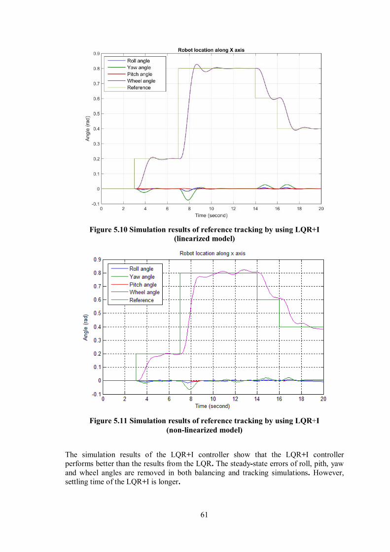
61  

 

Figure 5.10 Simulation results of reference tracking by using LQR+I (linearized model)

Figure 5.11 Simulation results of reference tracking by using LQR+I (non-linearized model)

 The  simulation  results  of  the  LQR+I  controller  show  that  the  LQR+I  controller performs better than the results from the LQR. The steady-state errors of roll, pith, yaw and  wheel  angles  are  removed  in  both  balancing  and  tracking  simulations. However, settling time of the LQR+I is longer. 

 

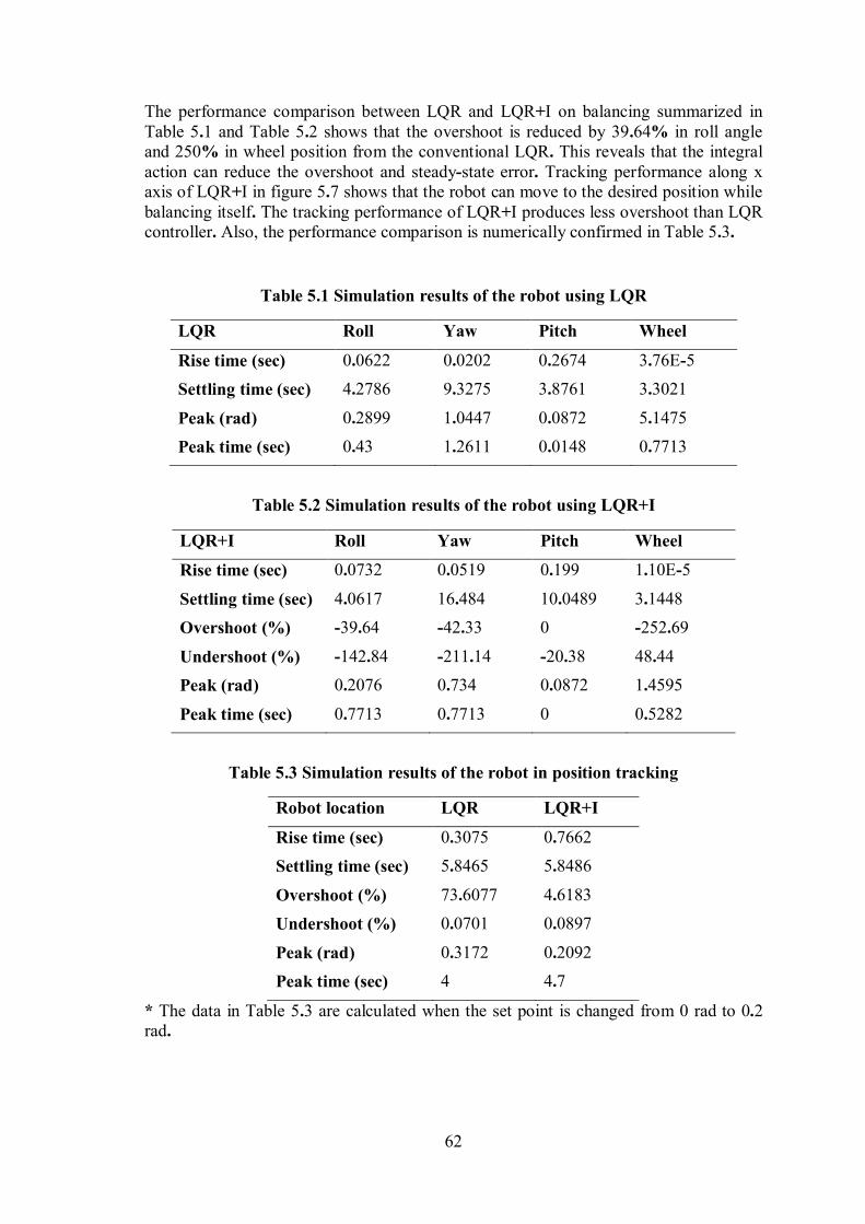
62  

The  performance  comparison  between  LQR  and  LQR+I  on  balancing  summarized  in Table 5.1 and Table 5.2 shows  that  the overshoot  is  reduced by 39.64% in  roll  angle and 250% in wheel position from the conventional LQR. This reveals that the integral action  can  reduce  the overshoot  and  steady-state error. Tracking  performance  along  x axis of LQR+I in figure 5.7 shows that the robot can move to the desired position while balancing itself. The tracking performance of LQR+I produces less overshoot than LQR controller. Also, the performance comparison is numerically confirmed in Table 5.3. 

Table 5.1 Simulation results of the robot using LQR

LQR Roll Yaw Pitch Wheel

Rise time (sec) 0.0622  0.0202  0.2674  3.76E-5 

Settling time (sec) 4.2786  9.3275  3.8761  3.3021 

Peak (rad) 0.2899  1.0447  0.0872  5.1475 

Peak time (sec) 0.43  1.2611  0.0148  0.7713 

Table 5.2 Simulation results of the robot using LQR+I

LQR+I Roll Yaw Pitch Wheel

Rise time (sec) 0.0732  0.0519  0.199  1.10E-5 

Settling time (sec) 4.0617  16.484  10.0489  3.1448 

Overshoot (%) -39.64  -42.33  0  -252.69 

Undershoot (%) -142.84  -211.14  -20.38  48.44 

Peak (rad) 0.2076  0.734  0.0872  1.4595 

Peak time (sec) 0.7713  0.7713  0  0.5282 

Table 5.3 Simulation results of the robot in position tracking

Robot location LQR LQR+I

Rise time (sec) 0.3075  0.7662 

Settling time (sec) 5.8465  5.8486 

Overshoot (%) 73.6077  4.6183 

Undershoot (%) 0.0701  0.0897 

Peak (rad) 0.3172  0.2092 

Peak time (sec) 4  4.7 

* The data in Table 5.3 are calculated when the set point  is changed  from 0 rad to 0.2 rad. 

     

 

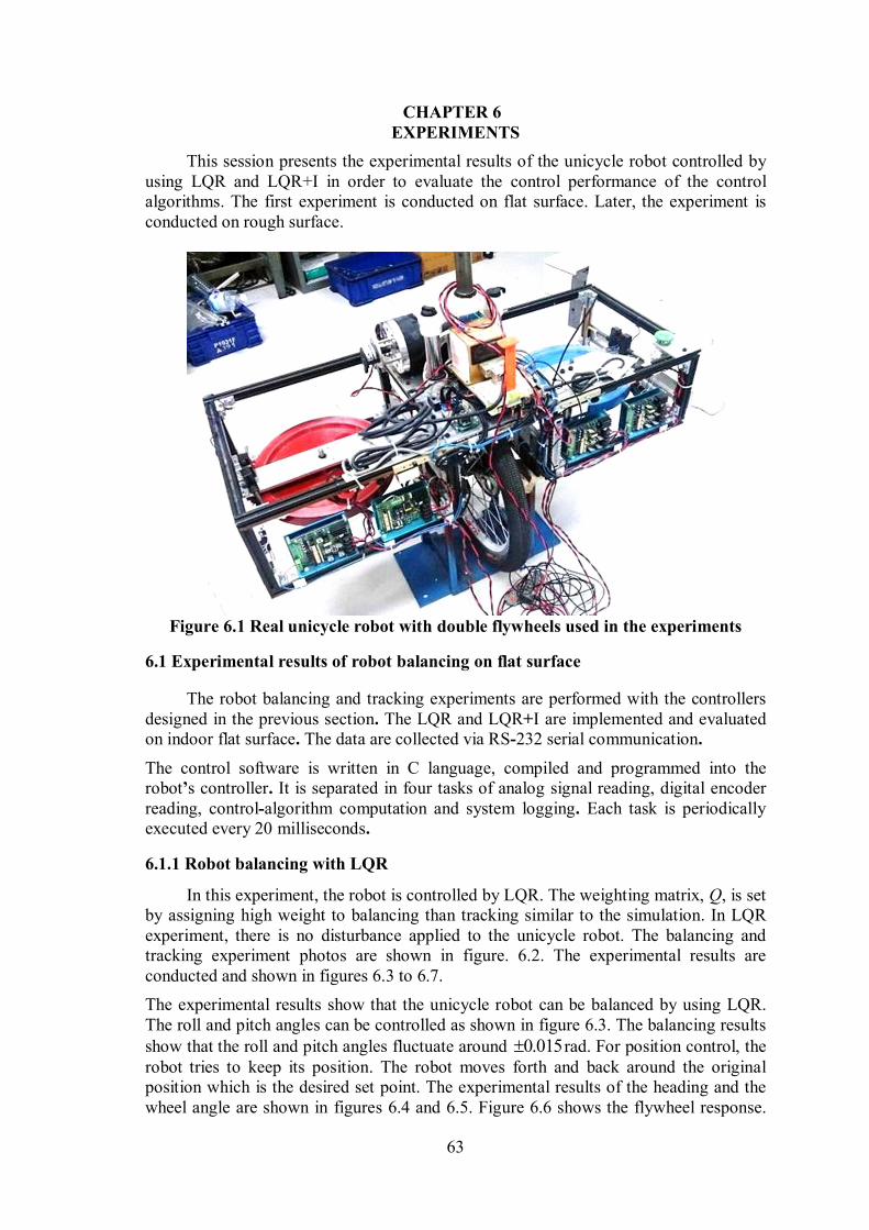
63  

CHAPTER 6 EXPERIMENTS

This session presents the experimental results of the unicycle robot controlled by using  LQR  and  LQR+I  in  order  to  evaluate  the  control  performance  of  the  control algorithms. The  first  experiment  is conducted on  flat  surface. Later, the experiment  is conducted on rough surface.  

 Figure 6.1 Real unicycle robot with double flywheels used in the experiments

6.1 Experimental results of robot balancing on flat surface

The robot balancing and tracking experiments are performed with the controllers designed in the previous section. The LQR and LQR+I are implemented and evaluated on indoor flat surface. The data are collected via RS-232 serial communication.  

The  control  software  is  written  in  C  language,  compiled  and  programmed  into  the robot’s controller. It is separated in four tasks of analog signal reading, digital encoder reading,  control-algorithm  computation  and  system  logging. Each  task  is  periodically executed every 20 milliseconds. 

6.1.1 Robot balancing with LQR

In this experiment, the robot is controlled by LQR. The weighting matrix, Q, is set by assigning high weight to balancing than tracking similar  to the simulation. In LQR experiment,  there  is  no  disturbance  applied  to  the  unicycle  robot.  The  balancing  and tracking  experiment  photos  are  shown  in  figure.  6.2.  The  experimental  results  are conducted and shown in figures 6.3 to 6.7. 

The experimental results show that the unicycle robot can be balanced by using LQR. The roll and pitch angles can be controlled as shown in figure 6.3. The balancing results show that the roll and pitch angles fluctuate around  0.015 rad. For position control, the robot  tries  to  keep  its  position.  The  robot  moves  forth  and  back  around  the  original position which is the desired set point. The experimental results of the heading and the wheel angle are shown in figures 6.4 and 6.5. Figure 6.6 shows the flywheel response. 

 

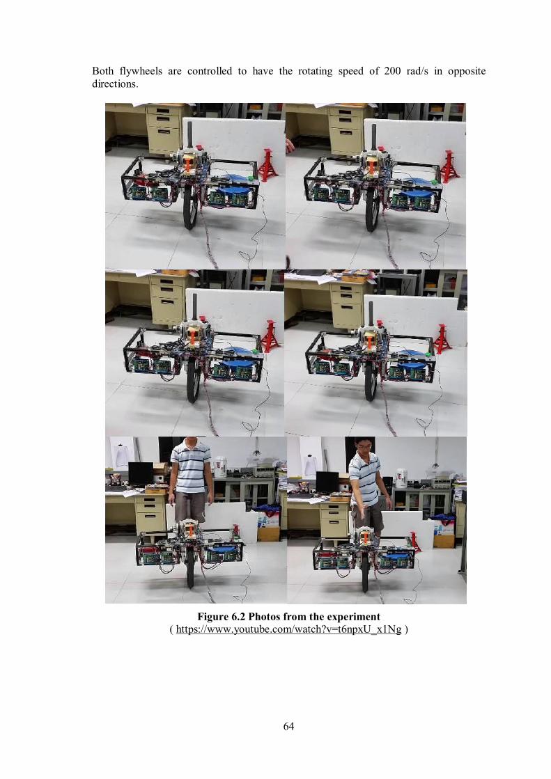
64  

Both  flywheels  are  controlled  to  have  the  rotating  speed  of  200  rad/s  in  opposite directions.  

 

Figure 6.2 Photos from the experiment  ( https://www.youtube.com/watch?v=t6npxU_x1Ng ) 

 

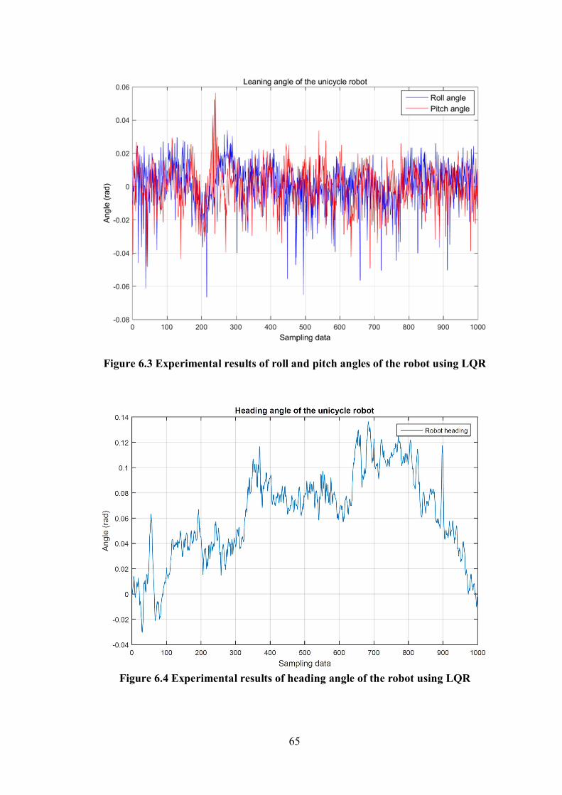
65  

Figure 6.3 Experimental results of roll and pitch angles of the robot using LQR 

  

 Figure 6.4 Experimental results of heading angle of the robot using LQR

 

 

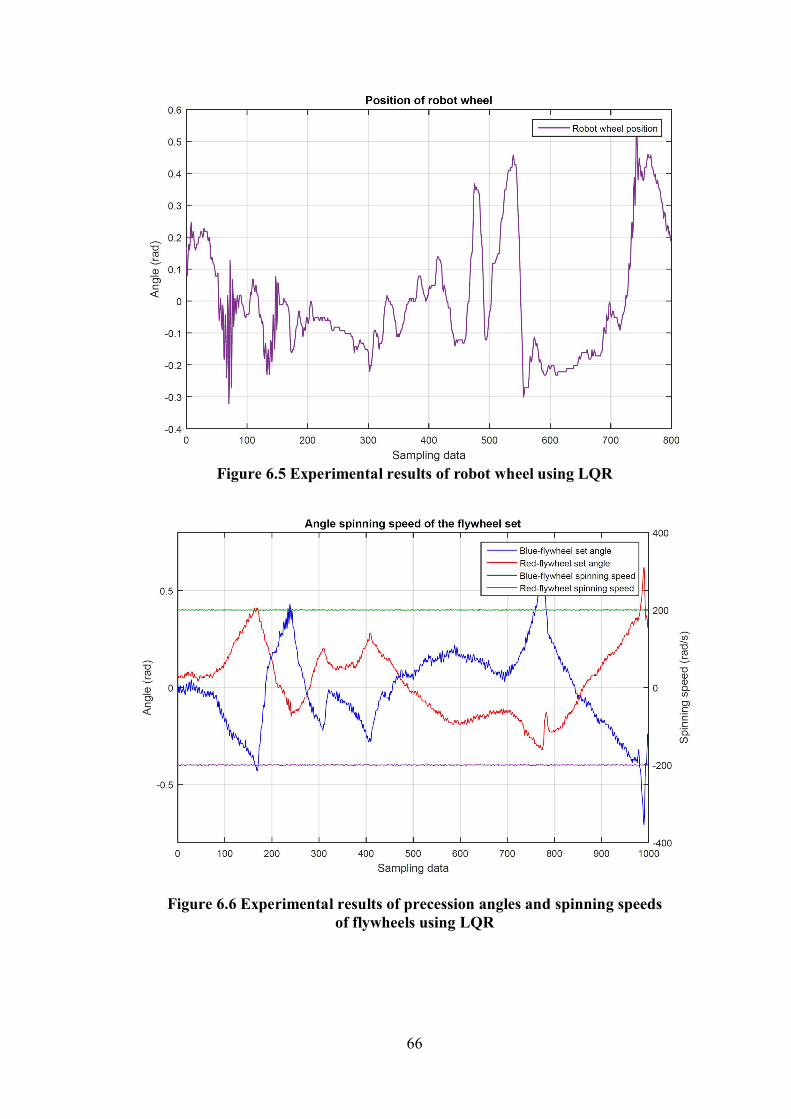
66  

 Figure 6.5 Experimental results of robot wheel using LQR

 

 

Figure 6.6 Experimental results of precession angles and spinning speeds of flywheels using LQR

 

 

 

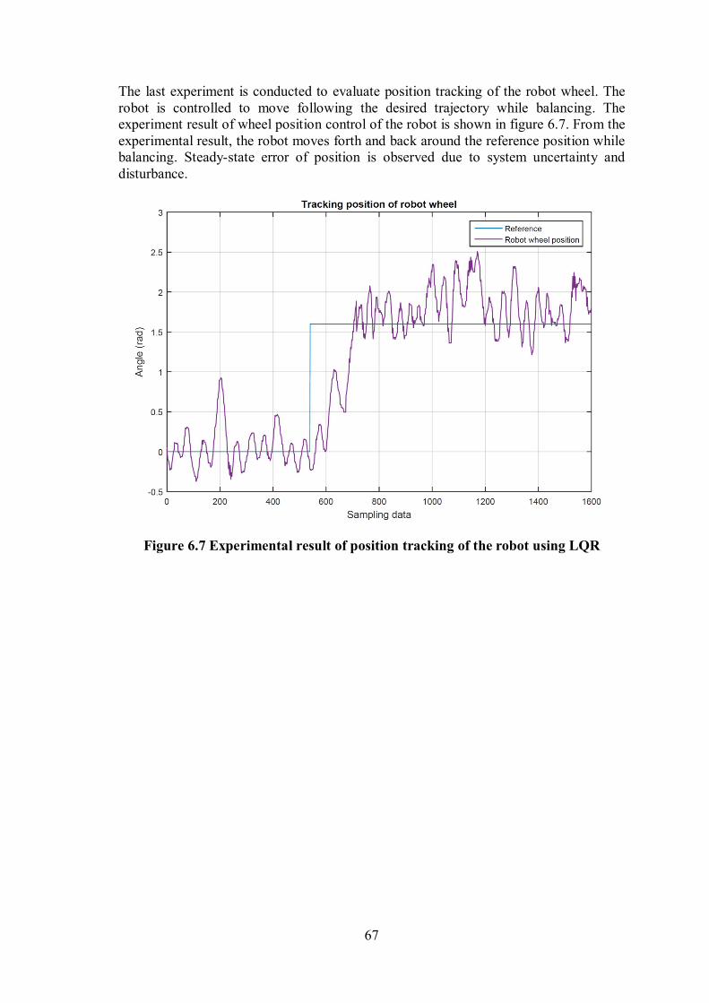
67  

The  last experiment  is conducted to evaluate position tracking of  the robot wheel. The robot  is  controlled  to  move  following  the  desired  trajectory  while  balancing.  The experiment result of wheel position control of the robot is shown in figure 6.7. From the experimental result, the robot moves forth and back around the reference position while balancing.  Steady-state  error  of  position  is  observed  due  to  system  uncertainty  and disturbance. 

 

Figure 6.7 Experimental result of position tracking of the robot using LQR

 

 

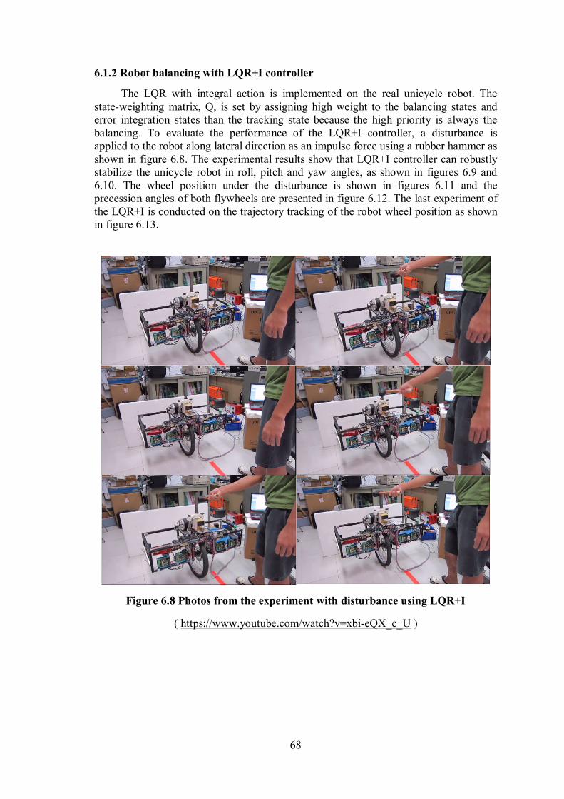
68  

6.1.2 Robot balancing with LQR+I controller

The  LQR  with  integral  action  is  implemented  on  the  real  unicycle  robot.  The state-weighting  matrix, Q,  is  set  by  assigning  high  weight  to  the  balancing  states  and error  integration  states  than  the  tracking  state  because  the  high  priority  is  always  the balancing.  To  evaluate  the  performance  of  the  LQR+I  controller,  a  disturbance  is applied to the robot along lateral direction as an impulse force using a rubber hammer as shown in figure 6.8. The experimental results show that LQR+I controller can robustly stabilize  the unicycle  robot  in  roll,  pitch and  yaw angles,  as  shown  in  figures 6.9 and 6.10.  The  wheel  position  under  the  disturbance  is  shown  in  figures  6.11  and  the precession angles of both flywheels are presented in figure 6.12. The last experiment of the LQR+I is conducted on the trajectory tracking of the robot wheel position as shown in figure 6.13. 

 

 

Figure 6.8 Photos from the experiment with disturbance using LQR+I

( https://www.youtube.com/watch?v=xbi-eQX_c_U )  

 

 

 

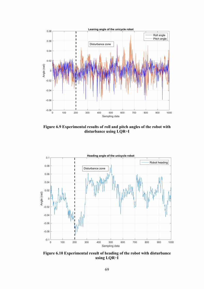
69  

 

Figure 6.9 Experimental results of roll and pitch angles of the robot with disturbance using LQR+I  

 

 

 Figure 6.10 Experimental result of heading of the robot with disturbance

using LQR+I 

 

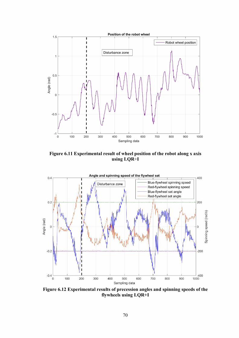
70  

 

Figure 6.11 Experimental result of wheel position of the robot along x axis using LQR+I

 

 Figure 6.12 Experimental results of precession angles and spinning speeds of the

flywheels using LQR+I

 

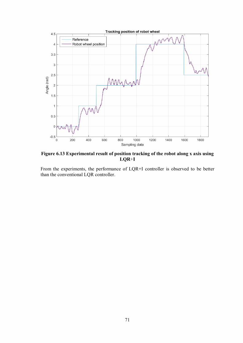
71  

 Figure 6.13 Experimental result of position tracking of the robot along x axis using

LQR+I 

From  the  experiments,  the  performance  of  LQR+I  controller  is  observed  to  be  better than the conventional LQR controller.     

 

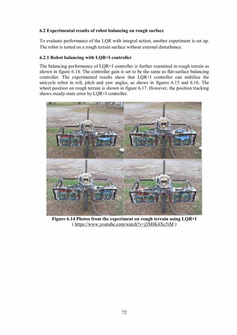
72  

6.2 Experimental results of robot balancing on rough surface

To evaluate performance of the LQR with integral action, another experiment is set up. 

The robot is tested on a rough terrain surface without external disturbance. 

6.2.1 Robot balancing with LQR+I controller

The balancing performance of LQR+I controller is further examined in rough terrain as shown in figure 6.14. The controller gain is set to be the same as flat-surface balancing controller.  The  experimental  results  show  that  LQR+I  controller  can  stabilize  the unicycle  robot  in  roll,  pitch  and  yaw  angles,  as  shows  in  figures  6.15  and  6.16.  The wheel position on rough terrain is shown in figure 6.17. However, the position tracking shows steady-state error by LQR+I controller.  

Figure 6.14 Photos from the experiment on rough terrain using LQR+I 

( https://www.youtube.com/watch?v=j3SHK4Xc5iM ) 

 

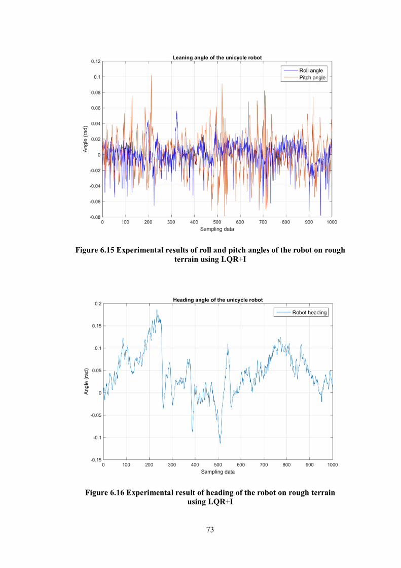
73  

Figure 6.15 Experimental results of roll and pitch angles of the robot on rough terrain using LQR+I 

  

 

Figure 6.16 Experimental result of heading of the robot on rough terrain using LQR+I 

 

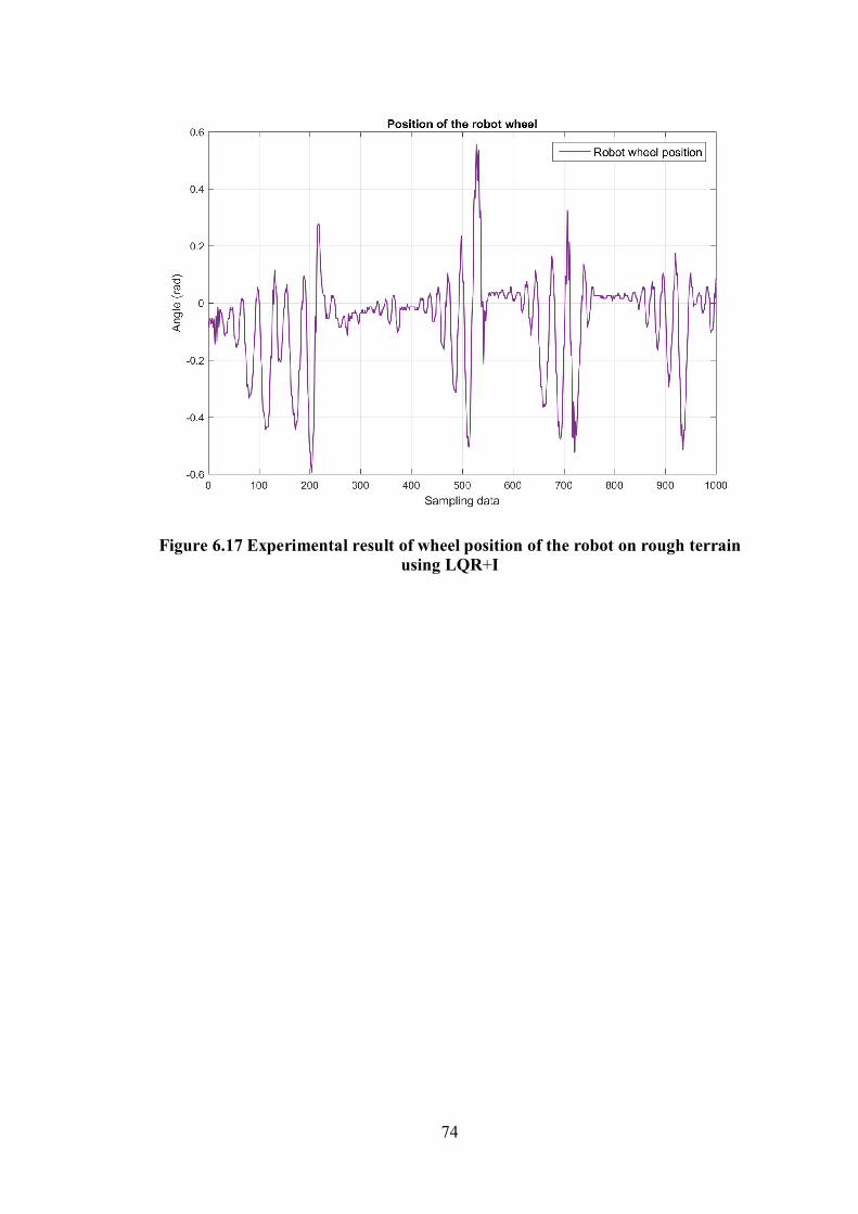
74  

 

Figure 6.17 Experimental result of wheel position of the robot on rough terrain using LQR+I

 

   

 

75  

CHAPTER 7 CONCLUSION AND FUTURE WORK

7.1 Conclusion

A  unicycle  robot  with  double  flywheels  was  proposed  in  this  dissertation.  Double flywheels  technique  was  designed  for  decoupling  the  robot’s  roll  and  heading  angles. By  using  double  flywheels,  the  rolling  torque  increases  compared  with  when  only  a single  flywheel  is used. Also,  the inverted-pendulum technique was applied to balance the robot’s pitch angle. Mechanism design and hardware architecture were explained in details. Dynamic model of  the unicycle robot was derived by using Euler-Lagrange method. It was  linearized  around  the  upright  position.  The  unicycle  robot  was  manufactured  and assembled. The  robot parameters were considered and  identified. 32 bits ARM  micro-controller  was  selected  to  control  the  unicycle  robot.  In  this  research,  the  control performance of the conventional LQR was compared with the proposed LQR+I by both simulations  and  experiments. The  LQR+I  showed  better  control  performance  than  the conventional  LQR.  The  LQR+I  could  effectively  reject  impact  disturbance  and eliminate  steady-state  error  as  seen  from  both  simulations  and  experiments.  In  the LQR+I  position  tracking,  the  robot  could  move  to  the  desired  position  and  maintain balancing  on  the  flat  surface.  Furthermore,  the  LQR+I  controller  could  balance  itself under  rough  terrain.  However,  position  tracking  on  rough  terrain  showed  steady-state error. It requires more robust controller than LQR+I.  

7.2 Future work

The unicycle robot with double flywheels was designed and developed in order to prove the  new  design  and  concept  of  roll,  pitch,  and  yaw  control  of  the  unicycle.  The  two flywheel  sets  were  located  at  the  left  and  the  right  of  the  robot's  body  in  order  to accommodate  calibration  and  adjustment.  In  the  further  improvement,  these  two flywheel  sets should  be  located as  a  stack  in  the  robot's  body  in order  to occupy  less space  and  the  motors  with  higher  power  should  be  selected  in  order  to  be  able  to balance and operate with passenger with weight up to 80 kg.     

 

76  

REFERENCES

[1]  Schoonwinkel  A. Design and  test of a computer stabilized unicycle. CA: Stan- ford University; 1987.  [2]  Sheng  Z,  Yamafuji  K.  Realization  of  a  human  riding  a  unicycle  by  a  robot.  In: IEEE international conference on robotics and automation, vol.2; 1995. p.1319–26.  [3]  Nakajima R, Tsubouchi T, Yuta S, Koyanagi E. A development of a new mech- anism of an autonomous unicycle. In: Proceedings of the 1997 IEEE/RSJ inter- national conference  on  intelligent  robots  and  systems.  Real-world  Application  IROS  ’97,  2; 1997. p.906–12.  [4]  Daud Y, Mamun AAl, Xu J-X. Properties of lateral-pendulum-controlled unicy- cle  robot  in  states  of  balance  and  motion.  In:  6th  IEEE  conference  on  robotics, automation and mechatronics; 2013. p. 162–7.  [5]  Lee JH, Shin HJ, Lee SJ,  Jung S. Balancing control of a  single-wheel  inverted pendulum  system  using  air  blowers:  evolution  of  Mechatronics  capstone  design. Mechatronics 2013; 23:926–32.  [6]  Majima S, Kasai T, Kadohara T. Design of a control method for changing yaw direction  of  an  underacuatted  unicycle  Robot.  In:  TENCON  2006  IEEE  Conference, vol. 10 ; 2006. p.1–4.  [7]  Majima S, Kasai T. A controller for changing the yaw direction of an underac- tuated  unicycle  robot.  In:  International  conference  on  technology  and  automation.,  vol. 5; 2005. p. 73–88.  [8]  Daoxiong  G,  Qi  P,  Guoyu  Z,  Xinghui  L.  LQR  control  for  a  self-balancing unicycle robot on inclined plane. J Syst Des Dyn 2012;6:685–99.  [9]  Xu  Y,  Au  SKW.  Stabilization  and  path  following  of  a  single  wheel  robot. IEEE/ASME Trans Mechatronics 2004;9:407–19.  [10]  Thanh BT, Parnichkun M. Balancing control of bicyrobo by particle swarm op- timization-based  structure-specified  mixed  H2/H∞  control.  Int  J  Adv  Robot  Syst 2008;5:395–402.  [11]  Lee J, Han S, Lee J. Decoupled dynamic control  for pitch and  roll  axes of  the unicycle robot. IEEE Trans Ind Electron 2013;60:3814–22.  [12]  Sheng Z, Yamafuji  K. Study of  stability and  motiom control of a unicycle  (5th report: Experimental results by fuzzy gain schedule PD controllers) Journal of robotics and mechatronics., vol. 8 ; 1996. p.571–9.  [13]  Caldecott  D,  Edwards  A,  Haynes  M,  Jerbic  M,  Kadis  A,  Madigan  R  and Cazzolato B. Modelling, simulation and control of an electric unicycle. In Proceedings 

 

77  

of Australasian Conference on Robotics and Automation, Brisbane, Australia., vol. 13; 2010.  [14]   Kappeler,  F.  Unicycle  robot.  Technical  report,  Automatic  Control  Laboratory, Ecole Polytechnique Federale de Lausanne, 2007 

 

 

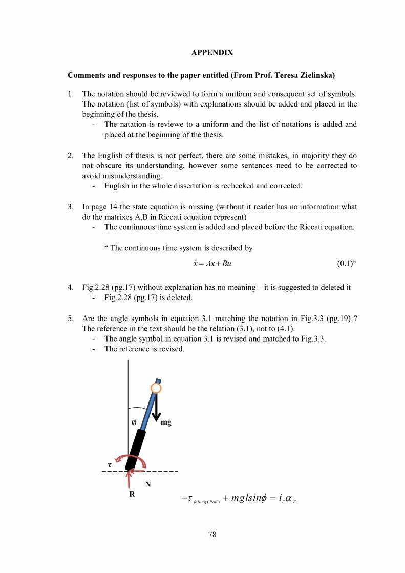
78  

APPENDIX

Comments and responses to the paper entitled (From Prof. Teresa Zielinska)  1. The notation should be reviewed to form a uniform and consequent set of symbols. 

The notation (list of symbols) with explanations should be added and placed in the beginning of the thesis. 

- The  natation  is  reviewe  to a uniform and  the  list of notations  is added and placed at the beginning of the thesis.  

2. The English of  thesis  is  not perfect,  there are  some  mistakes,  in  majority  they do not  obscure  its  understanding,  however  some  sentences  need  to  be  corrected  to avoid misunderstanding. 

- English in the whole dissertation is rechecked and corrected.  

3. In page 14 the state equation is missing (without it reader has no information what do the matrixes A,B in Riccati equation represent) 

- The continuous time system is added and placed before the Riccati equation.  

“ The continuous time system is described by 

  x Ax Bu            (0.1)” 

 4. Fig.2.28 (pg.17) without explanation has no meaning – it is suggested to deleted it 

- Fig.2.28 (pg.17) is deleted.  

5. Are  the angle  symbols  in  equation 3.1  matching  the notation  in  Fig.3.3  (pg.19)  ? The reference in the text should be the relation (3.1), not to (4.1). 

- The angle symbol in equation 3.1 is revised and matched to Fig.3.3. - The reference is revised. 

( )falling Roll F Fmglsin i  

�

N R

mg ∅

 

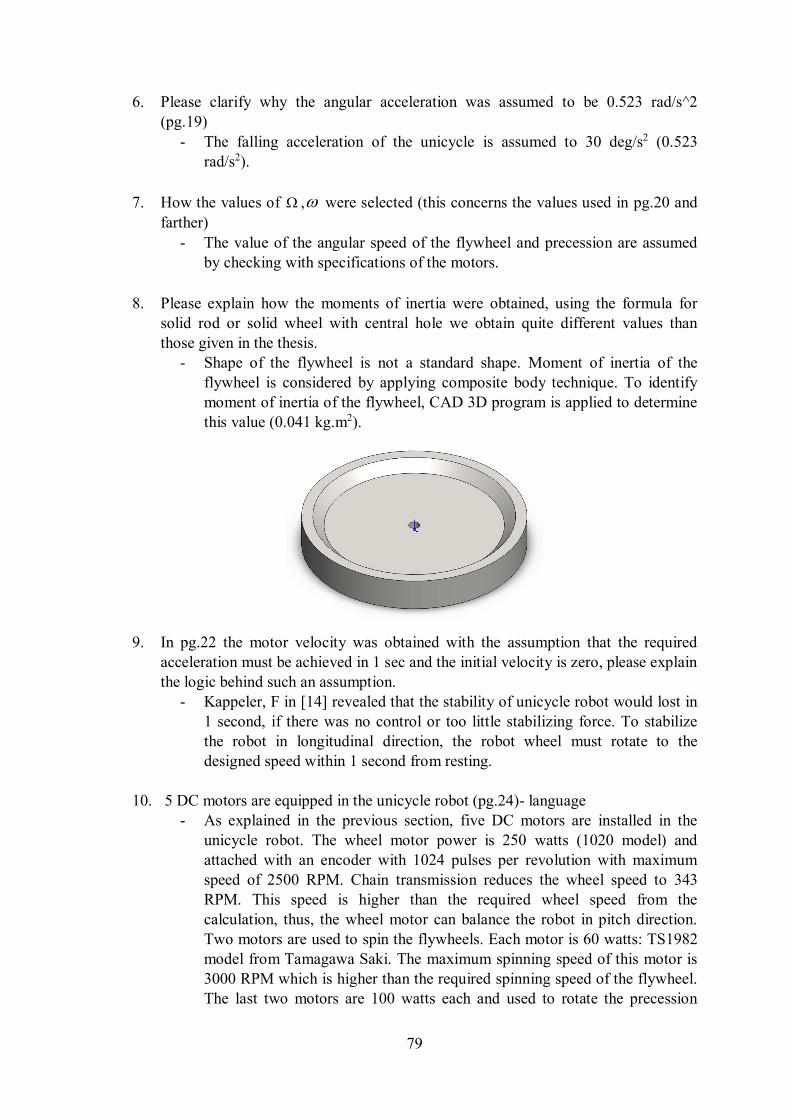
79  

6. Please  clarify  why  the  angular  acceleration  was  assumed  to  be  0.523  rad/s^2 (pg.19) 

- The  falling  acceleration  of  the  unicycle  is  assumed  to  30  deg/s2  (0.523 rad/s2).  

7. How the values of  ,  were selected (this concerns the values used in pg.20 and 

farther) 

- The value of  the angular speed of  the  flywheel and precession are assumed by checking with specifications of the motors.  

8. Please  explain  how  the  moments  of  inertia  were  obtained,  using  the  formula  for solid  rod  or  solid  wheel  with  central  hole  we  obtain  quite  different  values  than those given in the thesis. 

- Shape  of  the  flywheel  is  not  a  standard  shape.  Moment  of  inertia  of  the flywheel  is  considered  by  applying  composite  body  technique.  To  identify moment of inertia of the flywheel, CAD 3D program is applied to determine this value (0.041 kg.m2). 

 

9. In  pg.22  the  motor  velocity  was  obtained  with  the  assumption  that  the  required acceleration must be achieved in 1 sec and the initial velocity is zero, please explain the logic behind such an assumption. 

- Kappeler, F in [14] revealed that the stability of unicycle robot would lost in 1 second,  if  there was no control or  too little  stabilizing  force. To stabilize the  robot  in  longitudinal  direction,  the  robot  wheel  must  rotate  to  the designed speed within 1 second from resting.  

10.  5 DC motors are equipped in the unicycle robot (pg.24)- language - As  explained  in  the  previous  section,  five  DC  motors  are  installed  in  the 

unicycle  robot.  The  wheel  motor  power  is  250  watts  (1020  model)  and attached  with  an  encoder  with  1024  pulses  per  revolution  with  maximum speed  of  2500  RPM.  Chain  transmission  reduces  the  wheel  speed  to  343 RPM.  This  speed  is  higher  than  the  required  wheel  speed  from  the calculation,  thus,  the wheel  motor  can  balance  the  robot  in pitch direction. Two motors are used to spin the flywheels. Each motor is 60 watts: TS1982 model from Tamagawa Saki. The maximum spinning speed of this motor is 3000 RPM which is higher than the required spinning speed of the flywheel. The  last  two  motors  are  100  watts  each  and  used  to  rotate  the  precession 

 

80  

angle of each flywheel: Minertia DC motor, UGRMEM-02MA model. These motors are shown in figure 3.12. 

 

11.  In pg.22 the wheel motor speed 13.82 rpm was obtained, but it is not clear how in    the specification of motors (pg.24) the value from pg.22 was used. Please clarify 

- The detail is revised and presented in page 23. “Chain  transmission  reduces  the  wheel  speed  to  343  RPM  .This  speed  is higher  than  the  required  wheel  speed  from  the  calculation,  thus,  the  wheel motor can balance the robot in pitch direction.”  

12. In pg.25 not an electrical circuit, but electronic hardware is illustrated. - The electrical circuit is revised to electronic hardware 

 

13. What is the “signal controlling circuit” (pg.25) – I think that it is an amplifier - The circuit contains not only amplifier but also filter circuit. 

 

14. In pg.27,  it is stated that sensors monitoring part of the control system have lower 

acting priority than the controlling part – in that case how the timely response to the posture change detected by sensor in achieved? 

- The control law is repeated every 20 milliseconds by interrupt function from timer while sensors are monitored in looping of the main program. Sampling frequency of sensors monitoring is higher but less priority than control.  

15. Pg.28: “the robot wheel considered at the center of gravity of the wheel” ? - Revised “The robot wheel is considered as a point which locates at the center 

gravity of the wheel. Position vector from the origin point of the fixed world 

coordinate points to the center of the robot wheel (0

r ).” 

 

16. In  formulas  in  pg.28  and  pg.30  not  all  unit  vector  i,j,k  are  marked  by  dash, therefore  is  id  not  clear  if  x  and  y  in  both  equation  are  symbolizing  the  same quantity? Please clarify the notation with indication of the reference frames. 

- Revised (pg.28) 

˙

0

( )sin( )( )cos( ) ( )cos( )

( )cos( )

(

ˆ

)

ˆ

ˆ

w

y rsinV r x rsin rsin i j

rcos

rsin k

 

- Revised (pg.29) ' ' ' '˙

1 ' '

' ' ' '

Sin( )Sin( )Sin( ) Cos( )Sin( ) Cos( )Cos( )Sin( )

Cos( )Sin( ) Cos( )Cos( )Sin( )

Cos( )Sin( )Sin( ) Cos( )Cos( ) Cos( )Cos( )Cos( )

Sin( )Sin( )

F F

F

F

F F

x l r lV r i

r l

y l r l

r

' '

' ' '

Cos( )Sin( )Sin( )

Cos( )Sin( ) Sin( ) Cos( )Sin( )

F

F F

jl

l r l k

 

 

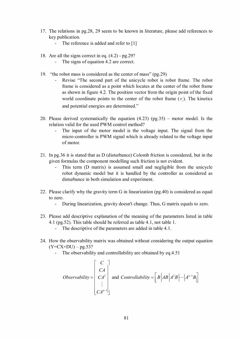
81  

17. The relations in pg.28, 29 seem to be known in literature, please add references to key publication. 

- The reference is added and refer to [1]  

18. Are all the signs correct in eq. (4.2) - pg.29? - The signs of equation 4.2 are correct. 

 

19.  “the robot mass is considered as the center of mass” (pg.29) - Revise  “The  second  part  of  the  unicycle  robot  is  robot  frame.  The  robot 

frame is considered as a point which locates at the center of the robot frame as shown in figure 4.2. The position vector from the origin point of the fixed 

world  coordinate  points  to  the  center  of  the  robot  frame  (1

r ).  The  kinetics 

and potential energies are determined.”  

20. Please  derived  systematically  the  equation  (4.23)  (pg.35)  –  motor  model.  Is  the relation valid for the used PWM control method? 

- The  input  of  the  motor  model  is  the  voltage  input.  The  signal  from  the micro-controller is PWM signal which is already related to the voltage input of motor.   

21. In pg.36 it is stated that as D (disturbance) Colomb friction is considered, but in the given formulas the component modelling such friction is not evident. 

- This  term  (D  matrix)  is  assumed  small  and  negligible  from  the  unicycle 

robot  dynamic  model  but  it  is  handled  by  the  controller  as  considered  as disturbance in both simulation and experiment.   

22. Please clarify why the gravity term G in linearization (pg.40) is considered as equal to zero. 

- During linearization, gravity doesn't change. Thus, G matrix equals to zero.   

23. Please add descriptive explanation of the meaning of the parameters listed in table 4.1 (pg.52). This table should be referred as table 4.1, not table 1. 

- The descriptive of the parameters are added in table 4.1.  

24. How the observability matrix was obtained without considering the output equation (Y=CX+DU) – pg.53? 

- The observability and controllability are obtained by eq.4.51 

2

1n

C

CA

Observability CA

CA

and  2 1nControllability B AB A B A B

 

 

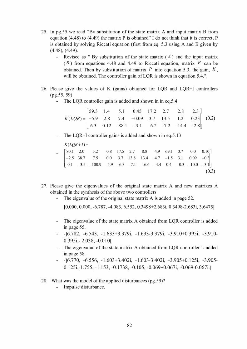
82  

25. In pg.55 we read  “By  substitution of  the state matrix  A and  input  matrix  B  from equation (4.48) to (4.49) the matrix P is obtained” I do not think that it is correct, P 

is obtained by solving Riccati equation (first from eq. 5.3 using A and B given by (4.48), (4.49). 

- Revised  as  "  By  substitution  of  the  state  matrix  ( A )  and  the  input  matrix  

( B )  from  equations  4.48  and  4.49  to  Riccati  equation,  matrix  P   can  be 

obtained. Then by substitution of matrix  P   into equation 5.3,  the gain,  K , will be obtained. The controller gain of LQR is shown in equation 5.4.".  

26. Please  give  the  values  of  K  (gains)  obtained  for  LQR  and  LQR+I  controllers  (pg.55, 59) 

- The LQR controller gain is added and shown in in eq.5.4 

59.3 1.4 5.1 0.45 17.2 2.7 2.8 2.3

( ) 5.9 2.8 7.4 0.09 3.7 13.5 1.2 0.23

6.3 0.12 88.1 3.1 6.2 7.2 14.4 2.8

K LQR

  (0.2) 

- The LQR+I controller gains is added and shown in eq.5.13 

-

( )

80.1 2.0 5.2 0.8 17.5 2.7 8.8 4.9 69.1 0.7 0.0 0.10

2.5 38.7 7.5 0.0 3.7 13.8 13.4 4.7 1.5 3.1 0.09 0.3

0.1 3.5 100.9 5.9 6.3 7.1 16.6 4.4 0.4 0.3 10.0 3.1

K LQR I

             (0.3) 

 

27. Please  give  the  eigenvalues  of  the  original  state  matrix  A  and  new  matrixes  A obtained in the synthesis of the above two controllers 

- The eigenvalue of the original state matrix A is added in page 52. 

[0.000, 0.000, -6.787, -4.083, 6.552, 0.3498+2.683i, 0.3498-2.683i, 3.6475] 

 

- The eigenvalue of the state matrix A obtained from LQR controller is added  in page 55. 

- ]- 6.782,  -6.543,  -1.633+3.379i,  -1.633-3.379i,  -3.910+0.395i,  -3.910-

0.395i,  - 2.038, -0.010[ 

- The eigenvalue of the state matrix A obtained from LQR controller is added  in page 58. 

- ]- 6.770,  -6.556,  -1.603+3.402i,  -1.603-3.402i,  -3.905+0.125i,  -3.905-

0.125i,-1.755, -1.153, -0.1738, -0.105, -0.069+0.067i, -0.069-0.067i.[  

28.  What was the model of the applied disturbances (pg.59)? - Impulse disturbance. 

     

 

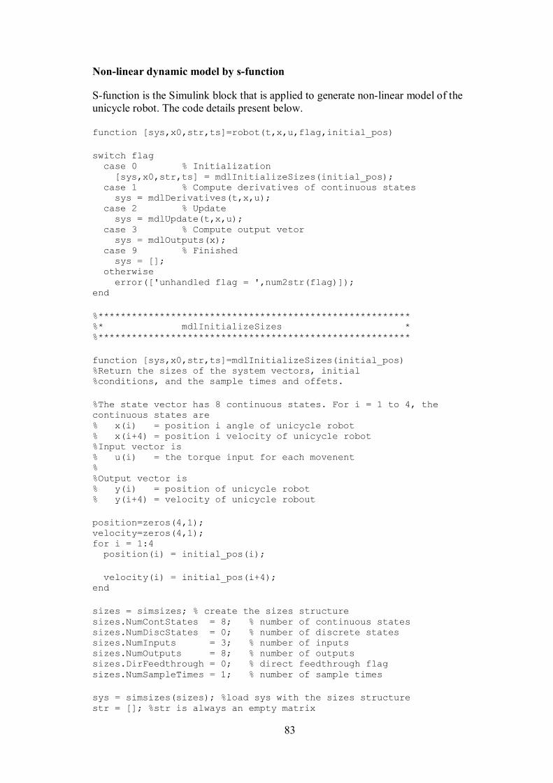
83  

Non-linear dynamic model by s-function

S-function is the Simulink block that is applied to generate non-linear model of the unicycle robot. The code details present below.  function [sys,x0,str,ts]=robot(t,x,u,flag,initial_pos) switch flag case 0 % Initialization [sys,x0,str,ts] = mdlInitializeSizes(initial_pos); case 1 % Compute derivatives of continuous states sys = mdlDerivatives(t,x,u); case 2 % Update sys = mdlUpdate(t,x,u); case 3 % Compute output vetor sys = mdlOutputs(x); case 9 % Finished sys = []; otherwise error(['unhandled flag = ',num2str(flag)]); end %******************************************************** %* mdlInitializeSizes * %******************************************************** function [sys,x0,str,ts]=mdlInitializeSizes(initial_pos) %Return the sizes of the system vectors, initial %conditions, and the sample times and offets. %The state vector has 8 continuous states. For i = 1 to 4, the continuous states are % x(i) = position i angle of unicycle robot % x(i+4) = position i velocity of unicycle robot %Input vector is % u(i) = the torque input for each movenent % %Output vector is % y(i) = position of unicycle robot % y(i+4) = velocity of unicycle robout position=zeros(4,1); velocity=zeros(4,1); for i = 1:4 position(i) = initial_pos(i); velocity(i) = initial_pos(i+4); end sizes = simsizes; % create the sizes structure sizes.NumContStates = 8; % number of continuous states sizes.NumDiscStates = 0; % number of discrete states sizes.NumInputs = 3; % number of inputs sizes.NumOutputs = 8; % number of outputs sizes.DirFeedthrough = 0; % direct feedthrough flag sizes.NumSampleTimes = 1; % number of sample times sys = simsizes(sizes); %load sys with the sizes structure str = []; %str is always an empty matrix

 

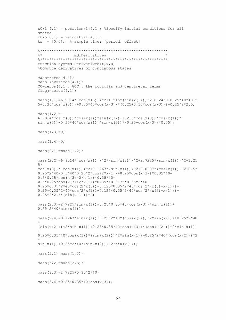
84  

x0(1:4,1) = position(1:4,1); %Specify initial conditions for all states x0(5:8,1) = velocity(1:4,1); ts = [0,0]; % sample time: [period, offset] %******************************************************** %* mdlDerivatives * %******************************************************** function sys=mdlDerivatives(t,x,u) %Compute derivatives of continuous states mass=zeros(4,4); mass_inv=zeros(4,4); CC=zeros(4,1); %CC : the coriolis and centipetal terms flagj=zeros(4,1); mass(1,1)=6.9014*(cos(x(3)))^2+1.215*(sin(x(3)))^2+0.2459+0.25*40*(0.25+0.35*cos(x(3)))+0.35*40*cos(x(3))*(0.25+0.35*cos(x(3)))+0.25^2*2.5; mass(1,2)=-6.9014*cos(x(3))*cos(x(1))*sin(x(3))+1.215*cos(x(3))*cos(x(1))* sin(x(3))-0.35*40*cos(x(1))*sin(x(3))*(0.25+cos(x(3))*0.35); mass(1,3)=0; mass(1,4)=0; mass(2,1)=mass(1,2); mass(2,2)=6.9014*(cos(x(1)))^2*(sin(x(3)))^2+2.7225*(sin(x(1)))^2+1.215* cos(x(3))*(cos(x(1)))^2+0.1267*(sin(x(1)))^2+0.0637*(cos(x(1)))^2+0.5*0.25^2*40-0.5*40*0.25^2*cos(2*x(1))+0.25*cos(x(3))*0.35*40-0.5*0.25*cos(x(3)-2*x(1))*0.35*40-0.5*0.25*cos(x(3)+2*x(1))*0.35*40+0.75*0.35^2*40-0.25*0.35^2*40*cos(2*x(3))-0.125*0.35^2*40*cos(2*(x(3)-x(1)))-0.25*0.35^2*40*cos(2*x(1))-0.125*0.35^2*40*cos(2*(x(3)+x(1)))+ 0.25^2*2.5*(sin(x(1)))^2; mass(2,3)=2.7225*sin(x(1))+0.25*0.35*40*cos(x(3))*sin(x(1))+ 0.35^2*40*sin(x(1)); mass(2,4)=0.1267*sin(x(1))+0.25^2*40*(cos(x(2)))^2*sin(x(1))+0.25^2*40* (sin(x(2)))^2*sin(x(1))+0.25*0.35*40*cos(x(3))*(cos(x(2)))^2*sin(x(1))+ 0.25*0.35*40*cos(x(3))*(sin(x(2)))^2*sin(x(1))+0.25^2*40*(cos(x(2)))^2* sin(x(1))+0.25^2*40*(sin(x(2)))^2*sin(x(1)); mass(3,1)=mass(1,3); mass(3,2)=mass(2,3); mass(3,3)=2.7225+0.35^2*40; mass(3,4)=0.25*0.35*40*cos(x(3));

 

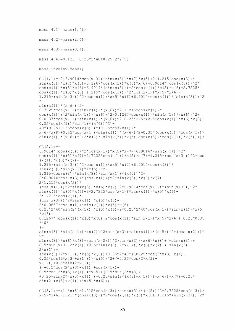
85  

mass(4,1)=mass(1,4); mass(4,2)=mass(2,4); mass(4,3)=mass(3,4); mass(4,4)=0.1267+0.25^2*40+0.25^2*2.5; mass_inv=inv(mass); CC(1,1)=-2*6.9014*cos(x(3))*sin(x(3))*x(7)*x(5)+2*1.215*cos(x(3))* sin(x(3))*x(7)*x(5)-0.1267*cos(x(1))*x(8)*x(6)-6.9014*(cos(x(3)))^2* cos(x(1))*x(5)*x(6)-6.9014*(sin(x(3)))^2*cos(x(1))*x(5)*x(6)-2.7225* cos(x(1))*x(5)*x(6)+1.215*(cos(x(3)))^2*cos(x(1))*x(5)*x(6)-1.215*(sin(x(3)))^2*cos(x(1))*x(5)*x(6)+6.9014*cos(x(1))*(sin(x(3)))^2* sin(x(1))*(x(6))^2-2.7225*cos(x(1))*sin(x(1))*(x(6))^2+1.215*cos(x(1))* cos(x(3)))^2*sin(x(1))*(x(6))^2-0.1267*cos(x(1))*sin(x(1))*(x(6))^2+ 0.0637*cos(x(1))*sin(x(1))*(x(6))^2-0.25*2.5*(2.5*cos(x(1))*x(6)*x(8)+ 0.25*cos(x(1))*sin(1)*(x(6))^2)-40*(0.25+0.35*cos(x(3)))*(0.25*cos(x(1))* x(6)*x(8)+0.25*cos(x(1))*sin(x(1))*(x(6))^2+0.35*(cos(x(3))*cos(x(1))* sin(x(1))*(x(6))^2+2*x(7)*(sin(x(3))*x(5)+cos(x(3))*cos(x(1))*x(6)))); CC(2,1)=-6.9014*(cos(x(3)))^2*cos(x(1))*x(5)*x(7)+6.9014*(sin(x(3)))^2* cos(x(1))*x(5)*x(7)+2.7225*cos(x(1))*x(5)*x(7)+1.215*(cos(x(3)))^2*cos(x(1))*x(5)*x(7)-1.215*(sin(x(3)))^2*cos(x(1))*x(5)*x(7)+6.9014*cos(x(3))* sin(x(3))*sin(x(1))*(x(5))^2-1.215*cos(x(3))*sin(x(3))*sin(x(1))*(x(5))^2+ 2*6.9014*cos(x(3))*(cos(x(1)))^2*sin(x(3))*x(6)*x(7)-2*1.215*cos(x(3))* (cos(x(1)))^2*sin(x(3))*x(6)*x(7)-2*6.9014*cos(x(1))*(sin(x(3)))^2* sin(x(1))*x(5)*x(6)+2*2.7225*cos(x(1))*sin(x(1))*x(5)*x(6)-2*1.215*cos(x(1))* (cos(x(3)))^2*sin(x(1))*x(5)*x(6)-2*0.0637*cos(x(1))*sin(x(1))*x(5)*x(6)+ 0.25^2*40*sin(2*(x(1)))*x(5)*x(6)+2*0.25^2*40*cos(x(1))*sin(x(1))*x(5)*x(6)+ 0.1267*(cos(x(1))*x(5)*x(8)+2*cos(x(1))*sin(x(1))*x(5)*x(6))+0.25*0.35*40* (-sin(x(3))*sin(x(1))*(x(7))^2+sin(x(3))*sin(x(1))*(x(5))^2+(cos(x(2)))^2* sin(x(3))*x(6)*x(8)+(sin(x(2)))^2*sin(x(3))*x(6)*x(8)+(-sin(x(3))+ 0.5*sin(x(3)-2*x(1))+0.5*sin(x(3)+2*x(1)))*x(6)*x(7)+(-sin(x(3)-2*x(1))+ sin(x(3)+2*x(1)))*x(5)*x(6))+0.35^2*40*((0.25*cos(2*x(3)-x(1))-0.25*cos(2*x(3)+x(1)))*(x(5))^2+(-0.25*cos(2*x(3)-x(1)))+0.5*sin(2*x(1))+ ((-0.5*cos(2*x(3)-x(1))+cos(x(1))-0.5*cos(2*x(3)+x(1)))*x(5)+(0.5*sin(2*x(3)) +0.25*sin(2*(x(3)-x(1)))+0.25*sin(2*(x(3)+x(1))))*x(6))*x(7)+0.25* sin(2*(x(3)+x(1)))*x(5)*x(6)); CC(3,1)=-(1)*x(8)-1.215*cos(x(3))*sin(x(3))*(x(5))^2+2.7225*cos(x(3))* x(5)*x(6)-1.215*(cos(x(3)))^2*cos(x(1))*x(5)*x(6)+1.215*(sin(x(3)))^2*

 

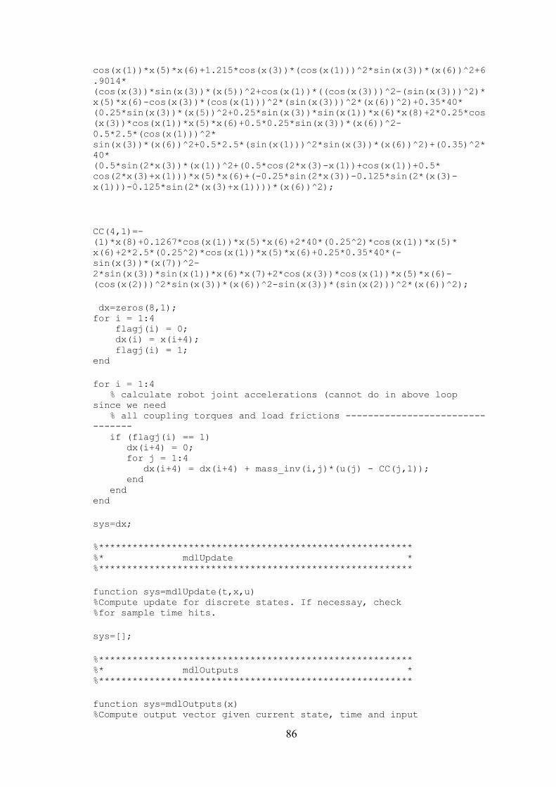
86  

cos(x(1))*x(5)*x(6)+1.215*cos(x(3))*(cos(x(1)))^2*sin(x(3))*(x(6))^2+6.9014* (cos(x(3))*sin(x(3))*(x(5))^2+cos(x(1))*((cos(x(3)))^2-(sin(x(3)))^2)* x(5)*x(6)-cos(x(3))*(cos(x(1)))^2*(sin(x(3)))^2*(x(6))^2)+0.35*40* (0.25*sin(x(3))*(x(5))^2+0.25*sin(x(3))*sin(x(1))*x(6)*x(8)+2*0.25*cos(x(3))*cos(x(1))*x(5)*x(6)+0.5*0.25*sin(x(3))*(x(6))^2-0.5*2.5*(cos(x(1)))^2* sin(x(3))*(x(6))^2+0.5*2.5*(sin(x(1)))^2*sin(x(3))*(x(6))^2)+(0.35)^2*40* (0.5*sin(2*x(3))*(x(1))^2+(0.5*cos(2*x(3)-x(1))+cos(x(1))+0.5* cos(2*x(3)+x(1)))*x(5)*x(6)+(-0.25*sin(2*x(3))-0.125*sin(2*(x(3)-x(1)))-0.125*sin(2*(x(3)+x(1))))*(x(6))^2);

CC(4,1)=-(1)*x(8)+0.1267*cos(x(1))*x(5)*x(6)+2*40*(0.25^2)*cos(x(1))*x(5)* x(6)+2*2.5*(0.25^2)*cos(x(1))*x(5)*x(6)+0.25*0.35*40*(-sin(x(3))*(x(7))^2-2*sin(x(3))*sin(x(1))*x(6)*x(7)+2*cos(x(3))*cos(x(1))*x(5)*x(6)-(cos(x(2)))^2*sin(x(3))*(x(6))^2-sin(x(3))*(sin(x(2)))^2*(x(6))^2); dx=zeros(8,1); for i = 1:4 flagj(i) = 0; dx(i) = x(i+4); flagj(i) = 1; end for i = 1:4 % calculate robot joint accelerations (cannot do in above loop since we need % all coupling torques and load frictions -------------------------------- if (flagj(i) == 1) dx(i+4) = 0; for j = 1:4 dx(i+4) = dx(i+4) + mass_inv(i,j)*(u(j) - CC(j,1)); end end end sys=dx; %******************************************************** %* mdlUpdate * %******************************************************** function sys=mdlUpdate(t,x,u) %Compute update for discrete states. If necessay, check %for sample time hits. sys=[]; %******************************************************** %* mdlOutputs * %******************************************************** function sys=mdlOutputs(x) %Compute output vector given current state, time and input

 

87  

position=zeros(4,1); velocity=zeros(4,1); for i = 1:4 position(i) = x(i); velocity(i) = x(i+4); end sys(1:4,1)=position; sys(5:8,1)=velocity;