Sliding-mode Velocity and Yaw Control of a 4WD Skid ... · Sliding-mode Velocity and Yaw Control of a ... of the partially linearized dynamics model of a unicycle robot. ... Dynamic

Sliding-mode Velocity and Yaw Control of a4WD Skid-steering Mobile Robot

Eric Lucet, Christophe Grand and Philippe Bidaud

Eric LucetRobosoft, Technopole d’Izarbel, F-64210 Bidart, France. e-mail: [email protected]

Christophe Grand and Philippe BidaudISIR-UPMC, UMR 7222, F-75005 Paris, France. e-mail: [email protected]

1

2 Eric Lucet, Christophe Grand and Philippe Bidaud

Abstract The subject of this paper is the design and implementation of a robustdynamic feedback controller, based on the dynamic model of the four-wheel skid-steering RobuFAST A robot, undergoing high-speed turns. The control inputs arerespectively the linear velocity and the yaw angle. The main objective of this paperis to formulate a sliding mode controller, robust enough to obviate the knowledgeof the forces within the wheel-soil interaction, in the presence of sliding phenom-ena and ground-level fluctuations. Finally, experiments are conduced on a slipperyground to ascertain the efficiency of the control law.

1 Introduction

This paper considers the problem of a robust control of high-speed wheeled robotsmaneuvering on slippery grounds with varying properties.

The dynamic control of skid-steering robots was studied in particular in [1] us-ing a dynamic feedback linearization paradigm for a model-based controller whichminimizes lateral skidding by imposing the longitudinal position of the instanta-neous center of rotation. Another algorithm reported in [2], offers a good robustnessconsidering uncertainties on the robot dynamic parameters. In addition to the non-holonomic constraint of the controller designed by Caracciolo, the authors use anoscillator signal [3] for kinematic control.

We suggest a strategy based on the sliding-mode theory. The sliding-mode con-trol law—or, more precisely, controller with variable structure generating a slidingregime—aims to obtain, by feedback, a dynamics widely independent from thatof the process and its possible variations. Hence, the controller can be consideredas belonging to the class of robust controllers. The sliding-mode control appearsattractive for the handling of nonlinear and linear systems, multivariable and single-variable systems, as well as model or trajectory pursuit problems and problems ofregulation.

Sliding-mode control allows a decoupling design procedure and good distur-bance rejection. This control scheme is robust to the uncertainties in the dynamicparameters of the system, and is easily implementable. Indeed, robust control iswidely used in the literature; particular [4] and [5] propose examples of dynamicsliding-mode controllers without taking into account the vehicle dynamics. In [6],and then [7], the authors consider the dynamics model of a unicycle system dur-ing the implementation of their control law by using the kinematic nonholonomicnon-skidding constraint. The non compliance with nonholonomic constraints in realconditions is taken into account in [8]. However, the problem is formalized for theparticular case of the partially linearized dynamics model of a unicycle robot.

Using the sliding-mode theory, we suggest here a new approach to control afast skid-steering mobile robot with wheel torques as inputs, based on its dynamicsmodel. The objective is to force the mobile robot to follow a desired path at rel-

Dynamic control of a 4WD skid-steering mobile robot 3

atively high speed, by controlling its yaw angle and its longitudinal velocity. Theground considered is nominally horizontal and relatively smooth as compared withthe wheel dimensions. If most of the control laws consider that the conditions ofmovement without slippage are satisfied, this hypothesis is not valid at high speed,where wheel slippage becomes significant, thus reducing the robot stability. Theimplemented controller will have to be robust with respect to these phenomena inorder to ensure an efficient path-following.

2 Application to a Skid-steering Mobile Robot

Because it has proved to be robust enough to obviate the modeling of the forcesin the wheel-soil interaction in the presence of slippage, a sliding-mode controlleris applied to a skid-steering mobile robot. This scheme ensures the control of thehending velocity and the yaw angle.

2.1 System Modeling

Considering the integer i ∈ [1;N] with N denoting the number of wheels of theskid-steering robot, let us define the two generalized torques τu and τθ , uniformlydistributed throughout the torques τi of each wheel i according to the equations:

τu =N

∑i=1

τi; τθ =N

∑i=1

−wi

Rτi (1)

y

x

y0

xx0O0

θτuτ

iτ

Fig. 1 Torques dispatching


2.2 Control of the Yaw Angle

2.2.1 Design of the Control Law

In the case of a skid-steering robot, let us express the yaw movement dynamics fromthe equations of the general dynamics:

Izr =N

∑i=1

(−wiFxi + liFyi) (2)

Applying Newton’s second law to the ith wheel, we have:

Iω ωi = τi−RFxi (3)

with R the wheel radius and Iw its centroidal moment of inertia, assumed to be thesame for all the wheels.

Considering the torque definition τθ and equations (3) and (2), we have :

r = λτθ +λθ ω +Dθ Fy (4)

with:

λ =1Iz

;λθ =Iω

IzR[· · ·wi · · ·] ; ω = [· · · ωi · · ·]T ;Dθ =

1Iz

[· · · li · · ·] ;Fy = [· · ·Fyi · · ·]T

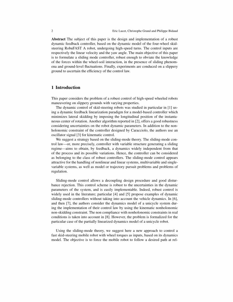
The correction of the vehicle steering does not permit the system to converge tothe desired trajectory. It is also necessary to correct the lateral error; otherwise, thesystem will aim towards a movement parallel to the reference path, not necessarilyreaching it. This is why we are going to modify the desired yaw angle, as proposedin other works [9].

The robot has to follow the path, the reference point P being all the time theprojection of its centre of mass G on this one. To take into account the lateral error,we add to θd a term limited between−π

2 and π

2 excluded, increasing with the lateralerror d, the function defining this term being also odd to permit a similar behavioron both sides of the path. We thus define the modified desired steering angle θd suchas:

θd = θd + arctan(

dd0

)(5)

with d0 a positive gain of regulation of the intensity of the correction of the lateraldistance d.

For the implementation of the controller, we proceed to a temporary change of thecontrol variable by replacing the generalized torque τθ . To this end, we introducecdθ , which represents the control law to be applied and n(θ ,r, r) the uncertaintyfunction on θ , r and r in the dynamics equations. We thus have the relation:


Fig. 2 Path following parameters

r = cdθ −n(θ ,r, r) (6)

The control law is chosen as:

cdθ = ˙rd +Kθp εθ +Kθ

d εθ +σθ (7)

which includes four terms:

• ˙rd , the second derivative of θd , an anticipative term;• εθ = θd−θ , the yaw-angle error;• Kθ

p and Kθd , two positive constants that permit to define the settling time and the

overshoot of the closed-loop system;• σθ , the sliding-mode control law.

2.2.2 Error State Equation

The second derivative of εθ is given below:

εθ = ˙rd− r = ˙rd− cdθ +n= ˙rd−

(˙rd +Kθ

p εθ +Kθd εθ +σθ

)+n

= −Kθp εθ −Kθ

d εθ +(n−σθ )(8)

Let the error state vector be: x =[

εθ , εθ

]T , the state equation then becoming

x = Ax+B(n−σθ ) (9)


with :

A =(

0 1−Kθ

p −Kθd

); B =

(01

)

If σθ = 0 (and so n = 0, without model error to correct), the system is linear,and we choose the values of Kθ

p and Kθd as Kθ

p = ω2n and Kθ

d = 2ζ ωn in order todefine a second-order system. ωn is the pulsation and ζ the damping ratio. To definenumerical values, the 5% settling time Tr is introduced: Tr = 4.2

ζ ωn.

2.2.3 Stability Analysis

To approach the problem of the stability of the closed-loop system, the pursuit ofthe desired yaw angle θd can be studied by using the candidate Lyapunov functionV = xT Px, with P a positive definite symmetric matrix. According to the Lyapunovtheorem, [10], the state x = 0 is stable if and only if:

V (0) = 0 ; ∀x 6= 0 V(x) > 0 and V(x) < 0 (10)

The first two foregoing relations being verified at once, it remains to establish thethird. From eq.(9), we compute the derivative:

V (x) = xT Px+xT Px=(xT AT +nBT −σθ BT

)Px+xT P(Ax+Bn−Bσθ )

= xT(AT P+PA

)x+2xT PB(n−σθ )

(11)

The last equality is obtained by considering that s = BT Px is a scalar, so BT Px =xT PB. Then, the matrix P is computed to obtain the equation (12) below:

AT P+PA =−Ql (12)

with Ql a positive defined symmetric matrix; it is the Lyapunov equation. In thatcase, the equation (11) is reformulated:

V =−xT Qlx+2xT PB(n−σθ )

It is necessary that V be negative for stability. The first term of the right-hand sideof the above equation is negative, while the second term vanishes if x lies in thekernel of BT P. Outside the kernel, the second term has to be as small as possible.Let us define s = BT Px. The equality s = 0 is the ideal case, represents the hyper-plane defining the sliding surface. Keeping the sliding surface s equal to zero is thenequivalent to the pursuit of the vector of the desired states, the error state vector xbeing zero. As this surface reaches the origin, the static error εθ will be equal tozero.


We suggest the sliding-mode control law σθ :

σθ = µs|s|

(13)

where we use the norm of s, and µ is a positive scalar. This choice leads to:

s(n−σθ ) = sn−µs2

|s|= sn−µ |s| ≤ |s|(|n|−µ)

Thus, the conditions of convergence are: |n| ≤ nMax < ∞ and a choice of µ > nMaxwhich guarantee the Lyapunov theorem hypotheses. Stability is guaranteed if weadopt the control law (13).

Finally, we have the control law:

cdθ = ˙rd +Kθp εθ +Kθ

d εθ + µs|s|

(14)

with s = BT Px.

2.2.4 Solution the Lyapunov Equation

To solve the equation (12), the matrix Ql is chosen as:

Ql =(

a 00 b

)with a > 0 and b > 0. With matrix A determined, matrix P is:

P =

(1.05bζ 2Tr

+ 5aζ 2Tr21 + aTr

16.8aζ 2Tr

2

35.28aζ 2Tr

2

35.28bTr16.8 + aζ 2T 3

r296.352

)(15)

We determine the influence of the Ql matrix components. As previously defined, theequation of the sliding hyperplane is:

s = BT Px = p21εθ + p22εθ

with p21 and p22 being two entries of the positive-definite and symmetric matrix Poccurring in the expression of the candidate Lyapunov function. Here, this hyper-plane is a straight line.

At the neighborhood of this straight line, we have: s = p21εθ + p22εθ = 0, whoseintegral is:

εθ (t) = εθ (τ)exp[(−p21

/p22)(t− τ)

]


with εθ (τ) a real constant which depends on the initial conditions at t = τ , whenthe system arrives at the neighborhood of the sliding straight line.

Consequently, we derive from this solution that to correct the error, it is necessaryto increase the value of p21 and to decrease the value of p22. According to expression(15) for P, we know these two parameters. Hence, to eliminate quickly the positionerror, it is necessary to increase the value of a and to decrease that of b. As far asthe sliding straight line is concerned, this modification of the various coefficientsincreases the straight line slope.

2.3 Control of the Longitudinal Velocity

We use the dynamics model according to the longitudinal axis from the equationsof the general dynamics:

M (u− rv) =N

∑i=1

Fxi (16)

From the definition of the torque τu and equations (3) and (16), we solve for thelongitudinal acceleration:

u = γτu +Λu

N

∑i=1

ωi + rv (17)

with:γ =

1MR

; Λu =−Iω

MR

As stated previously, cu is the control law and m(u, u) is a function of uncertain-ties on u and u in the equations of the system dynamics. We have the followingrelationship:

u = cu−m(u, u) (18)

with the control law defined as:

cu = ud +Kupεu +σu (19)

and:

• ud , an anticipative term;• εu = ud−u, the velocity error;• Ku

p, a positive constant that permits to define the settling time of the closed-loopsystem;

• σu, the sliding-mode control law.


Using the Lyapunov candidate function V =(1/

2)

ε2u , it can be immediately veri-

fied that the stability of the system is guaranteed by the choice of the sliding-modecontrol lawσu = ρ

εu|εu| , with ρ a positive scalar, large enough to compensate the

uncertainties on the longitudinal dynamics of the system.

2.4 Expression of the Global Control Law

In practice, uncertainty about the dynamics of the system to control leads to un-certainty in the sliding hyperplane s = 0. As a consequence s 6= 0 and the slidingcontrol law s, which has a behavior similar to the signum function, induces oscilla-tions while trying to reach the sliding surface s = 0 with a theoretically zero time.These high-frequency oscillations around the sliding surface, called chattering, in-crease the energy consumption and can damage the actuators. In order to reducethem, we can replace the signum function by an arctan function or, as chosen here,by adding a parameter with a small value ν in the denominator. So, we use the func-tion s

|s|+ν.

Finally, the following torques are applied to each of the N wheels:

τi =1N

(τu−

Rwi

τθ

)(20)

with τu and τθ re-computed with a change of variable, from the inverse of the robotdynamics model—equations (17) and (4) with the accelerations u and θ replacedrespectively by the control laws (19) and (14)—namely,

τu =1γ

(ud +Ku

pεu +ρεu

|εu|+νu−Λu

N

∑i=1

ωi− rv

)(21)

τθ =1λ

(˙rd +Kθ

p εθ +Kθd εθ + µ

BT Px|BT Px|+νθ

−Λθ ω−Dθ Fy)

(22)

To estimate the value of the lateral forces Fy, Pacejka theory [11] could be used,by taking into account the slip angle. Because of the robustness of the sliding-modecontrol, however we can consider that Fy is a perturbation to be rejected, and wedo not include it in the control law. A slip-angle measure being in practice not veryefficient, this solution is better.


3 Application to the RobuFAST A Robot

3.1 Experiments

3.1.1 Control Law Implementation

The sliding-mode control law is tested with the RobuFAST A robot on a slipperyflat ground. This experimental platform, shown in Fig.3, consists of an electric off-road vehicle, whose maximum reachable speed is 8 m/s. Designed for all-terrainmobility, the robot can climb slopes of up to 45◦ and has the properties displayedin Table 1. The front and rear directions of the vehicle are blocked to allow theskid-steering mode operation.

Total mass M = 350 kgYaw inertia Iz = 270 kg.m2

Wheelbase l = 1.2 mRear half-wheelbase w = 0.58 m

Table 1 Experimental robot inertial parameters

The implementation of the control law in real-life conditions requires some mea-sures and observations. In particular the norm of the velocity vector, measured bythe GPS, must be decomposed into its lateral and longitudinal components. Thisdecomposition is made possible by the addition of an observer of the slippage angle[12], the knowledge of this angle and the velocity vector norm allowing us to makea projection on the axes of the robot frame.

The controller is implemented in two steps: first, a proportional derivative con-troller is settled for path following; then, the sliding-mode controller is added andits gains tuned.

This sliding-mode controller being a torque controller, a difficulty is that therobuFast A robot inputs are its wheel velocities. It is thus necessary to convert theamplitude of the torques generated by the controller.

Referring to eq.(3) of the wheel dynamics, we can consider that the addition of aforce differential in a wheel is equivalent to a differential in its angular acceleration,i.e.,

∆ω ≡ RIω

∆F

The losses in the movement transmission, due to wheel-soil contact, are disturbancesto be compensated by the robust controller. This method is justified in particular ina patent [13].

The value of Iω is obtained by the sum Iω = Ieq + I′ω . For a Marvilor BL 72 motorof a mass of 2.06kg and a reduction gear with K = 16, we have Iω = 0.364kg.m2,


where I′ω is the wheel inertia and Ieq = K2Im is the inertia equivalent to the motorand reduction gear unit, with K the reduction gear speed reducing ratio and Im themotor inertia.

3.1.2 Experiment Results

The robot moves at a velocity of 3 m/s along a sinusoidal road. A derivative-proportional controller is applied to the robot, then the sliding-mode controller isimplemented.

The position is plotted on figure 4 in m, the gains being tuned for optimum path-following: Ku

p = 0.05 s−1, Kθd = 0.02 s−1, Kθ

p = Kθd

2/4ζ 2, ζ = 0.70, Tr = 0.5 s,

νu = 0.01 ms−1, νθ = 0.02, a = 0.10, b = 0.1, µ = 0.1 and ρ = 0.01 ms−2.

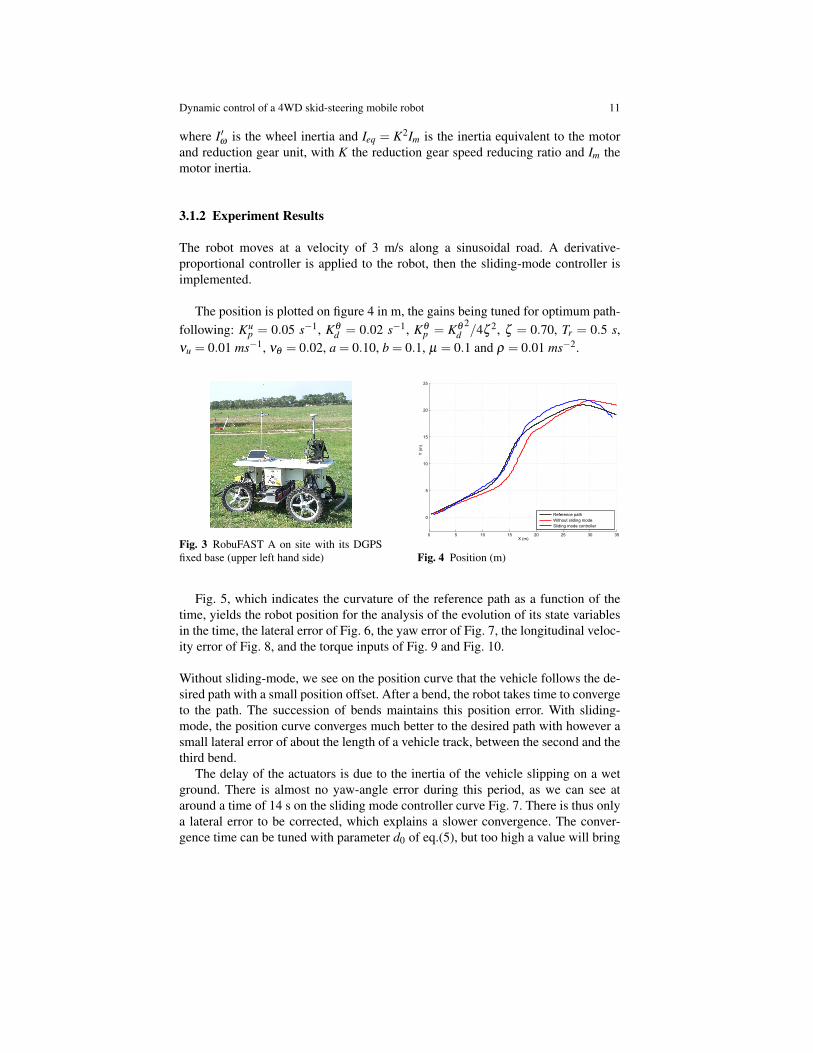
Fig. 3 RobuFAST A on site with its DGPSfixed base (upper left hand side) Fig. 4 Position (m)

Fig. 5, which indicates the curvature of the reference path as a function of thetime, yields the robot position for the analysis of the evolution of its state variablesin the time, the lateral error of Fig. 6, the yaw error of Fig. 7, the longitudinal veloc-ity error of Fig. 8, and the torque inputs of Fig. 9 and Fig. 10.

Without sliding-mode, we see on the position curve that the vehicle follows the de-sired path with a small position offset. After a bend, the robot takes time to convergeto the path. The succession of bends maintains this position error. With sliding-mode, the position curve converges much better to the desired path with however asmall lateral error of about the length of a vehicle track, between the second and thethird bend.

The delay of the actuators is due to the inertia of the vehicle slipping on a wetground. There is almost no yaw-angle error during this period, as we can see ataround a time of 14 s on the sliding mode controller curve Fig. 7. There is thus onlya lateral error to be corrected, which explains a slower convergence. The conver-gence time can be tuned with parameter d0 of eq.(5), but too high a value will bring


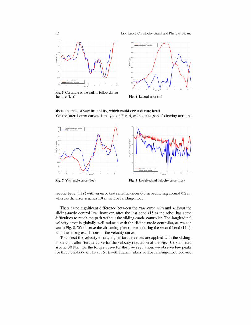
Fig. 5 Curvature of the path to follow duringthe time (1/m) Fig. 6 Lateral error (m)

about the risk of yaw instability, which could occur during bend.On the lateral error curves displayed on Fig. 6, we notice a good following until the

Fig. 7 Yaw angle error (deg) Fig. 8 Longitudinal velocity error (m/s)

second bend (11 s) with an error that remains under 0.6 m oscillating around 0.2 m,whereas the error reaches 1.8 m without sliding-mode.

There is no significant difference between the yaw error with and without thesliding-mode control law; however, after the last bend (15 s) the robot has somedifficulties to reach the path without the sliding-mode controller. The longitudinalvelocity error is globally well reduced with the sliding-mode controller, as we cansee in Fig. 8. We observe the chattering phenomenon during the second bend (11 s),with the strong oscillations of the velocity curve.

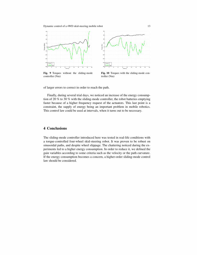
To correct the velocity errors, higher torque values are applied with the sliding-mode controller (torque curve for the velocity regulation of the Fig. 10), stabilizedaround 30 Nm. On the torque curve for the yaw regulation, we observe few peaksfor three bends (7 s, 11 s et 15 s), with higher values without sliding-mode because


Fig. 9 Torques without the sliding-modecontroller (Nm)

Fig. 10 Torques with the sliding-mode con-troller (Nm)

of larger errors to correct in order to reach the path.

Finally, during several trial days, we noticed an increase of the energy consump-tion of 20 % to 30 % with the sliding-mode controller, the robot batteries emptyingfaster because of a higher frequency request of the actuators. This last point is aconstraint, the supply of energy being an important problem in mobile robotics.This control law could be used at intervals, when it turns out to be necessary.

4 Conclusions

The sliding-mode controller introduced here was tested in real-life conditions witha torque-controlled four-wheel skid-steering robot. It was proven to be robust onsinusoidal paths, and despite wheel slippage. The chattering noticed during the ex-periments led to a higher energy consumption. In order to reduce it, we defined thegain variables according to some criteria such as the velocity or the path curvature.If the energy consumption becomes a concern, a higher-order sliding-mode controllaw should be considered.


References

1. L. Caracciolo, A. De Luca, and S. Iannitti. Trajectory tracking control of a four-wheel differ-entially driven mobile robot. In Proceedings of the IEEE International Conference on Robotics& Automation, pages 2632–2638, Detroit, Michigan, May 1999.

2. K. Kozlowski and D. Pazderski. Modeling and control of a 4-wheel skid-steering mobile robot.International journal of applied mathematics and computer science, 14:477–496, 2004.

3. W.E. Dixon, D.M. Dawson, E. Zergeroglu, and A. Behal. Nonlinear Control of WheeledMobile Robots. London, 2001.

4. A. Jorge, B. Chacal, and H. Sira-Ramirez. On the sliding mode control of wheeled mobilerobots. In Systems, Man, and Cybernetics, 1994. ’Humans, Information and Technology’.,IEEE International Conference on, volume 2, pages 1938–1943, Oct 1994.

5. L. E. Aguilar, T. Hamel, and P. Soueres. Robust path following control for wheeled robots viasliding mode techniques. In IROS, 1997.

6. J.-M. Yang and J.-H. Kim. Sliding mode control for trajectory tracking of nonholonomicwheeled mobile robots. In IEEE, 1999.

7. M.L. Corradini and G. Orlando. Control of mobile robots with uncertainties in the dynamicalmodel: a discrete time sliding mode approach with experimental results. In Elsevier ScienceLtd., editor, Control Engineering Practice, volume 10, pages 23–34. Pergamon, 2002.

8. F. Hamerlain, K. Achour, T. Floquet, and W. Perruquetti. Higher order sliding mode control ofwheeled mobile robots in the presence of sliding effects. In Decision and Control, and 2005European Control Conference. CDC-ECC ’05. 44th IEEE Conference on, pages 1959–1963,12-15 Dec. 2005.

9. D. Lhomme-Desages, Ch. Grand, and J.C. Guinot. Trajectory control of a four-wheel skid-steering vehicle over soft terrain using a physical interaction model. In Proceedings ofICRA’07 : IEEE/Int. Conf. on Robotics and Automation, pages 1164 – 1169, Roma, Italy,April 2007.

10. S. S. Sastry. Nonlinear systems: Analysis, Stability and Control. Springer Verlag, 1999.11. H. B. Pacejka. Tyre and vehicle dynamics. 2002.12. C. Cariou, R. Lenain, B. Thuilot, and M. Berducat. Automatic guidance of a four-wheel-

steering mobile robot for accurate field operations. J. Field Robot., 26:504–518, 2009.13. T. Yoshikawa. Open-loop torque control on joint position controlled robots, October 2008.

Documents

Sliding-mode Velocity and Yaw Control of a 4WD Skid ... · Sliding-mode Velocity and Yaw Control of a ... of the partially linearized dynamics model of a unicycle robot. ... Dynamic