The Demand for PBS Medicine - Victoria Universityvuir.vu.edu.au/15935/1/15935.pdf · The Demand for PBS Medicine ... including the fact that the income elasticity for necessities

The Demand for PBS Medicine

Kim Sweeny Centre for Strategic Economic Studies, Victoria University

Working Paper No. 45 Centre for Strategic Economic Studies Victoria University Melbourne April 2009

PO Box 14428 Melbourne VIC 8001 Australia Telephone +613 9919 1340 Fax +613 9919 1350 Contact: [email protected]


CSES Working Paper No. 45 1

The Demand for PBS Medicines

1 Introduction

In a change that attracted virtually no comment, the Department of Health Care and

Ageing (DoHA) announced in December 2005 that the Safety Net thresholds for the

Pharmaceutical Benefits Scheme (PBS) would be increased by an amount equal to

two additional copayments for each of the years from 2006 to 2009. The then

Coalition government claimed that this would “…help to rebalance the way costs for

the PBS as a taxpayer-funded scheme are shared between the government and

individuals” (DoHA 2005). Although denounced by the then Opposition as “ripping a

hole in the PBS Safety Net” (Parliamentary Library 2005), the Labor Government has

retained this policy change which was expected to save the Government about $140

million over 4 years. Perhaps the muted response to these changes is because patients,

particular those that are chronically ill, are not organized politically to respond to

policy changes that affect them adversely. In addition the significance of these

changes may not have been apparent at the time they were made.

When purchasing PBS medicines, patients pay a fixed copayment (plus any price

premium added by suppliers above the listed base price). For general patients who

comprise about 75% of the population the copayment in 2009 is $32.90, while for

concessional patients (such as pensioners and other health care cardholders) it is

$5.30. Under the Safety Net provisions, general patients pay the concessional

copayment once their expenditure on PBS medicines has reached the Safety Net

threshold (SNT), while concessional patients pay nothing after the threshold is

reached. In 2009, the SNT for general patients is $1264.90 or 38.5 copayments, and

for concessional patients $318.00 or 60 copayments. Changes to copayments and

Safety Net thresholds are the chief policy mechanisms that influence the cost of PBS

medicines to patients and might be expected to affect the willingness and ability of

patients to purchase them. This therefore raises questions about how well the

Commonwealth Government can meet the objectives of its National Medicines Policy



to ensure “timely access to the medicines that Australians need, at a cost individuals

and the community can afford” (Department of Health and Aged Care 2000).

The purpose of this paper is to quantify the impact of changes in copayments and

SNTs and other factors on the amount of PBS medicines consumed by patients by

estimating demand functions for different categories of PBS patients.

An important consideration in estimating equations based on observed values for

quantity and prices in markets is to what extent the data results from demand factors

alone or from the interaction of both demand and supply factors. For PBS medicines,

suppliers effectively enter a contract with the Government to provide sufficient

medicines at the listed price to meet demand. The amount supplied is therefore not

dependent on the price so the supply schedule is horizontal. In a very few instances

suppliers have withdrawn medicines when they can no longer agree with the

Government about the price but this still means the supply schedule is horizontal

while the medicine is listed on the PBS.

A few suppliers have entered into risk-sharing agreements which specify that once a

threshold demand has been reached there is some adjustment in remuneration

typically by a reduction in a price. However in most cases the threshold is not reached

so the provisions are not invoked. In any case the causation is from consumer demand

to price whereas the usual assumption about the supply schedule is that changes in

price lead to changes in supply behaviour. In these conditions the supplier still agrees

to provide medicines at the new price to meet the demand. For these reasons, there

can be considerable confidence that equations estimated with observed market data

are demand functions.

The following section is taken up with a brief review of demand models and

concludes that a simplified model of demand for PBS medicines can be adopted

because the operations of the PBS make certain of the considerations considered

important in the literature, such as the estimation of cross-price elasticities

unnecessary.



The next section presents a review of four previous studies of the demand for PBS

medicines concentrating on the estimates of elasticities with respect to prices

(typically the copayments) and of income.

This is followed by a section reporting the results of regression analysis of the

demand for PBS medicines by four categories of PBS patients, namely the two types

of patients split into the two safety net categories. These patient categories are

therefore:

General non-safety net (GNSN)

General safety net (GSN)

Concessional non-safety net (CNSN)

Concessional safety net (CSN)

This classification into four categories enables the influence of the safety net limits to

be better assessed and shows how the different patient categories react to changes in

the factors influencing demand. It should be recognised that GSN and CNSN patients

both face the same concessional copayment but will have different aggregate patient

prices because the influence of the premium will vary due to the two patient

categories having different consumption patterns. For CSN patients there will be no

price effect. The results of some regressions are discussed in the paper but are not

reported in the tables. These results are available from the author.

Medicines available under the PBS are published in the Schedule of Pharmaceutical

Benefits for Approved Pharmacists and Medical Practitioners (DoHA 2007) which

specifies among other things the price and conditions under which PBS medicines can

be prescribed and dispensed. Each particular combination of form and strength of a

brand of medicine is allocated a separate PBS item code and most of the analysis in

this paper is conducted at the level of the PBS item.



2 Demand models

The starting point for most expositions of demand analysis is the Marshallian demand

function which relates an individual’s consumption of a particular good to the price of

the good (its own price), the prices of other goods, and income, namely

( , )iq f M p (1.1)

where iq is the amount of good i consumed, 1

n

i ii

M p q

is the consumer’s income,

and p is a vector of prices of both good i and competing goods.

The difficulty with estimating a set of demand equations of the form (1.1) is that the

vector of prices for competing goods is large making it virtually impossible to

estimate both the own and cross-price elasticities, even if individuals are aggregated.

To make the task more tractable, the consumer’s purchases are segregated into groups

with discrete budgets and while there is substitution of products within groups there is

little if any substitution among groups. This means that the demand function for a

particular product can be specified with a limited number of competing products and

all other products can be ignored.

There are a number of competing functional forms for equation (1.1) but as Rosenthal

et al (2003) observe “none has yet been shown to be superior in estimating demand

models in markets for prescription drugs” (p 9).

The most common approach is to estimate the demand function for a particular good

or set of goods on a stand-alone basis without reference to the demand for other goods

and without trying to make the results compatible with the theory of consumer

demand. The most common specification for equation (1.1) is the double logarithmic

form

1 1

log log log logn m

i i i ij i ik ikj k

q M p z

(1.2)

where kz z is a vector of m other variables that influence the demand for good i.

One of the attractions of this form is that the coefficients of the variables are

elasticities, so that i is the income elasticity of demand, ii is the own price



elasticity, ij is the cross price elasticity with respect to good j, and ik is the elasticity

with respect to the k’th other factor.

It is not possible to ensure that the double logarithmic form (1.2) will produce

estimates of the coefficients that will conform to the restrictions on parameters

suggested by consumer demand theory, namely adding-up, homogeneity, symmetry

and negativity.

Because of this a number of approaches have been developed which attempt to either

ensure or impose these restrictions or at least test their validity. Clements,

Selvanathan and Selvanathan (1996) provide a relatively recent review of these

alternative demand systems and discuss various functional forms and their

derivations. Deaton and Muellbauer (1980a) also summarise the literature to that date.

The description below draws mainly on these two sources.

One of the earliest approaches was the linear expenditure system (LES) of Stone

(1954) in which the equation for the i’th product is

1

( )n

i i i i i j ij

p q p M p

(1.3)

where 0i and i iq are constants.

While straightforward to use, the LES specification has a number of drawbacks,

including the fact that the income elasticity for necessities rises with income, while

the income elasticity of luxuries falls.

The Rotterdam model was developed by Barten (1964) and Theil (1975) and in its

finite form is given by

1

log log ( log log )n

it it i t ij jt tj

w q Q p P

(1.4)

where the average budget share is 1

2it it

it

w ww

,

is the difference operator defined as 1t t tx x x ,



tQ is defined as the consumer’s real income ie tt

t

MQ

P , or log logt t tlogQ M P ,

1

log logn

j jj

P w p

is the Divisia price index, and

1

log logn

t i iti

P p

.

Equation (1.4) can be expressed in a somewhat simpler form as

1

log log logn

it it i t ij jtj

w q Q p

(1.5)

The Almost Ideal Demand System (AIDS) was developed by Deaton and Muellbauer

(1980b) and has the form

1

log logn

i i i ij jj

Mw p

P

(1.6)

but now P has a more complicated form given by

*0

1 1 1

1log log log log

2

n n n

k k kj j kk k j

P p p p

Deaton and Muellbauer suggest that in most circumstances it is possible to replace P

by an appropriate price index such as the Divisia index given above. The first

difference form of (1.6) is

1

log logn

i i ij jj

Mw p

P

(1.7)

Recognising that M

QP

, this can be rewritten as

1

log logn

i i ij jj

w Q p

(1.8)

Comparing equations (1.5) and (1.8) shows that in first difference form the Rotterdam

and AIDS models differ just in the form of the dependent variable. For the Rotterdam

model the dependent variable is the difference in the logs of quantities weighted by

value share while for the AIDS model it is just the value share.



In summary then there are a number of ways of specifying demand functions where

either the quantity demanded or the share in expenditure is expressed as a function of

income and own and competing good pricesi.

When applied to the demand for PBS medicines, these equations can be simplified to

a great extent by recognising that the only “own price” that will have any influence on

the patient’s demand for a particular medicine is the relevant copayment for that class

of patient and any premium that may be added by the manufacturer to the medicine.

The combination of copayment and premium is highly correlated with just the

copayment itself which therefore means that all own prices must be highly correlated

with competing prices – an outcome almost guaranteed by the operation of reference

pricing within the PBS. The consequence is that only one price is required in the

demand equation, namely the own price which is just the copayment plus premium (or

the copayment by itself).

3 Previous studies of the demand for PBS medicines

Estimates of the impact of changes in copayments and other factors on the demand for

PBS medicines have been undertaken by other researchers, notably Harvey (1984),

Bureau of Industry Economics (BIE) (1985), Johnston (1990) and McManus et al

(1996). Typically these studies concentrate on periods when there have been

significant changes in the copayments.

Harvey (1984) provides estimates of both price and income elasticities for general

patients firstly for the period 1967-68 to 1979-80 using annual data and secondly

using monthly data for two periods – 1969-70 to 1971-72 and 1974-75 to 1976-77.

For his first set of estimates he specifies two forms of the demand equation a log-log

version

1 2 3

5 6

log log log log

(1 ) log logit t t t

i it it it

GR a PR a WR a DR

r a ADDR a DELR u

(1.9)

and a log-linear version



1 2 3 4

5 6

log

log logit t t t

it it it

GR a P a W a D a

a ADDR a DELR e

(1.10)

where itGR is the ratio of per capita use of general prescriptions at time t and t-1 for

the i’th therapeutic group, tPR is the ratio of deflated patient contributions, tWR is the

ratio of deflated AWE, tDR is the ratio of the ratio of doctors per 100,000 population

and ADDR and DELR are terms to account for the addition and deletion of new

medicines.

Harvey uses annual data on the number of prescriptions for general patients for 19

broad therapeutic groups for the years 1968-69 to 1979-80. He presents results based

on using all the data within a single equation but for different intervals within the

overall period. For the log-log specification all coefficients on the price variable are

insignificant and are mostly insignificant for the doctor ratio variable. The income

elasticity however is positive, generally significant and varies between 1.5 and 2.5.

The log-linear version produces similar outcomes although the income elasticity is

smaller and less significant, the price elasticity is somewhat more significant but has

t-values less than or equal to 1.5, and the doctor variable generally has the wrong sign.

In a third set of estimates Harvey uses monthly prescription data on 13 medicines in

four therapeutic groups for two periods July 1970 to June 1973 and July 1974 to June

1977 and for all months combined. He estimates equations for each medicine

separately and for each of the four groups. Here however the equation is specified in

levels form unlike the ratio form used in the previous analysis. Looking at the results

for all months there are negative and significant elasticities for price for 7 of the 13

medicines, a positive and significant coefficient for the income elasticity for 1

medicine and a positive and significant coefficient for the doctor variable for 4

medicines. Where significant the price elasticity was in the range -0.1 to -0.2. For the

four groups the price elasticity was negative and significant for 2 groups (diuretics

and urinary antiseptics but not tetracyclines or penicillins) in the range -0.08 to -0.14.

In summary, the evidence for a significant copayment elasticity is poor at the overall

level and mixed at the detailed medicine level. Where present it lies in the range -0.1



to -0.2. By contrast the income elasticity is evident at the aggregate level but not at the

detailed level and the doctor variable generally performs poorly.

The BIE (1985) estimates the demand for total PBS prescriptions per capita for non-

pensioners using a simple linear equation with the copayment and average weekly

earnings (AWE) as explanatory variables along with two different measures of doctor-

patient contacts. Both the copayment and AWE are expressed in real terms and annual

data from 1959-60 to 1980-81 is used. Based on the coefficients obtained the BIE

estimate the elasticity with respect to the copayment as either -0.17 or -0.25 and the

income elasticity as “around 3” (p85).

Johnston (1990) examines the effect of the doubling of the general copayment from

$5 to $10 that occurred in November 1986 along with the introduction of the safety

net. At this time pensioners continued to receive medicines free so the safety net of 25

prescriptions applied only to general and concessional patients. For both safety net

groups medicines were then free – the copayment for general safety net patients was

only introduced in 1991. At the same time the concessional copayment was raised

from $2.00 to $2.50 but Johnston ignores this in his analysis. The doubling of the

general copayment effectively introduced the problem that purchases of PBS

medicines with prices below the general copayment level by general non-safety net

patients were not recorded. Prior to that, according to Johnston, “in practice very few

prescriptions dispensed to general patients attracted a charge of less than $5.00”. To

simplify his analysis, Johnston only considers the demand by general patients for

medicines costing more than $10. This comprises some 340 items from a total of

around 1200 at that time. He uses two sets of data – the first is for the four months

from May to August in 1986 and 1987, i.e. before and after the increase in copayment,

while the second is for the 24 months from May 1987 to April 1989. It should be

noted that there was a further increase in the general copayment to $11 in July 1988

which is not considered.

Because the data on prescription use by safety net patients provided to him does not

distinguish between former general and concessional patients Johnston uses the

second dataset to estimate for each item how many general patient prescriptions fell

into the safety net category after adjusting for the increase in demand by safety net



patients paying a lesser copayment. Using these estimates he adjusts the data for the

first dataset and estimates an equation relating the number of adjusted prescriptions in

1987 to actual prescriptions in 1986. Based on this he estimates a very significant fall

of 26.6% in general patient prescriptions due to the doubling of the general

copayment, or an (uncompensated arc) elasticity of -0.47 for medicines costing more

than $10. Using the second dataset he estimates the increase in general safety net

patient use as 64% when moving from the copayment of $10 to zero, or an arc

elasticity of -0.24. The elasticities are “uncompensated” because the procedure does

not allow the calculation of an income elasticity.

McManus et al (1996) examine the impact on prescription use of the change in the

general copayment from $11 to $15 in November 1990 (an increase of 36.4%) along

with the introduction of a copayment of $2.50 for pensioners. The concessional

copayment was unchanged. They also consider the effect on Repatriation patients of

the introduction of a $2.50 copayment in January 1992. For both pensioners and

Repatriation patients a compensating pharmaceutical allowance equal to 52

copayments per year was added to pensions. Unlike the other studies, McManus et al

use the data on total community use based on the DUSC dataset published as

Australian Statistics on Medicine (DoHA 2007a). This includes a component

estimated from a survey of pharmacies for general non-safety net usage of medicines

with a price below the general copayment. The data is monthly from July 1989 to

September 1994 for the analysis of the demand for general prescriptions and from

July 1987 to September 1994 for the Repatriation patients. Again there are further

changes to general and concessional copayments and safety net levels during the

period which are not considered within the analysis.

McManus et al define two categories of medicines – the first is “essential” medicines

in 12 therapeutic groups primarily used for treating chronic conditions such as

hypertension while the second consists of medicines in 9 therapeutic groups for

“discretionary” conditions such as antihistamines. While the description is a little

unclear, they appear to estimate equations for the two types of medicines where the

dependent variable is the level of prescriptions and the explanatory variables are the

underlying trend prior to change in the copayment, change in prescriptions after

change in the copayment, the underlying trend after change and a “pulse” term to



control for an anticipatory increase in prescriptions just prior to the change. Based on

the coefficients obtained, they find that community prescriptions for “discretionary

medicines” were 24.8% lower than might have been expected without any change in

the copayment, while the change for “essential” medicines was 18.1%. They also

report that regression results for 9 of the 12 essential therapeutic groups estimated

individually showed similar results to the aggregate results. They do not provide

similar results for the Repatriation patients, although they report decreases in the level

of prescriptions for both “essential” and “discretionary” categories.

This review of four studies provides mixed evidence of the impact of copayments on

consumption of medicines although all find some effect at least within certain

categories of medicines. Harvey, BIE and Johnston are necessarily restricted to

estimating copayment elasticities for general patients and report values from -0.1 to -

0.47 with most estimates being in the range -0.2 to –0.25. McManus et al do not

report elasticities and do not distinguish between general and concessional patients,

but find a differential response for categories of medicines. Only Harvey and BIE

attempt to estimate an income elasticity and the values for this range between 1.5 and

3. None of the studies includes restriction levels or other influences except for the

number of doctors which proves to be irrelevant.

4 Econometric analysis of the demand for PBS medicines

In undertaking an analysis of the demand for PBS medicines decisions must be made

about a number of factors that will influence the scope and nature of the project.

These largely revolve around the level of aggregation for the analysis, the choice of

variables to include, and the specification of the equation.

At one extreme it is possible to envisage separate equations being estimated for each

PBS item. This is impractical for reasons other than the amount of resources required

to do it. At most the number of annual observations available is 15 while for a

majority of items the actual number will be significantly less with many having only a

handful of observations. This means that it would be difficult to obtain meaningful

estimates for the coefficients of variables within these equations.



One way of approaching the problem is to recognise that the market for PBS

medicines is made up of a number of therapeutic treatment markets each of which is

composed of medicines that are close substitutes in the treatment of a particular

disease or condition but have limited use if any outside this treatment area. These

markets can be defined in a number of ways, for instance by using the Anatomical

Therapeutic Classification (ATC) maintained by the WHO Collaborating Centre for

Drug Statistics Methodology (2007). The ATC is defined at different levels and at the

more detailed levels (ATC3, ATC4, ATC5) encompasses various therapeutic markets.

The analysis of pharmaceutical markets has usually been confined to treatments for

specific conditions and has usually concentrated on estimating the demand for the

these treatments as a whole and then separately estimating shares of medicines within

the group. Cockburn and Anis (2001) have used this approach in their analysis of the

market for arthritis medicines in the USA, as have Berndt et al (1994), Suslow (1996),

and Berndt et al (1999) in their analyses of the market for anti-ulcer medicines. The

market for antidepressants has been examined similarly by Berndt et al (2002),

Cleanthous (2004), and Donohue and Berndt (2006) and Ellison and Hellerstein

(1999) have applied this to the market for antibiotics.

The challenge with estimating demand equations for suitably defined groups of

medicines is how to construct the aggregate quantity variable. One way is to use the

number of units for each medicine and aggregate them using the Defined Daily Dose

(DDD) equivalences published by the WHO Collaborating Centre but for some

groups of medicines these are not defined. An alternative is to calculate quantity

indexes based on the items within a group and use this as the quantity measure. While

aggregation will result in more groups having a larger number of observations, there

will still be relatively recent groups of medicines that will have significantly fewer

observations than might be desired. Even if the chosen aggregation level is ATC3, this

would still involve estimating over 70 equations.

Beyond a certain level of aggregation (such as ATC3 or ATC4) however the degree of

substitutability among medicines diminishes sharply and it is not obvious what a

quantity measure based on either DDDs or an index would be measuring.



A detailed analysis of the demand for groups of PBS medicines is beyond the scope of

this paper so two relatively simple approaches are used to gain some insights into the

impact of various factors on the demand for PBS medicines by different types of

patients.

The first approach is based on three alternative measures of the total quantity of PBS

medicines consumed using annual data for the years from 1991-92 to 2005-06. The

first quantity measure is the total number of units (such as tablets, capsules etc) of

medicine calculated by multiplying the number of scripts at the PBS item level by the

maximum quantity for that item in the particular year and then summing across items.

The second measure is a quantity index calculated for the relevant patient group and

the third is the total expenditure for the patient category deflated by a price index

calculated for that category. These last two quantity measures are quality-adjusted

indicators of consumption. Further information on the construction of these price and

quantity indexes is given in Sweeny (2009).

The explanatory variables considered consist of measures of price and income, as well

as three other potential influences on demand: the number of PBS medicines (defined

as distinct chemical or molecular entities rather than items) available in a particular

year, measures of restriction levels and the effect of safety net limits. Two variants of

the price variable are tested – the relevant patient price index which includes the

effect of both the relevant copayment and any price premium, and just the copayment

itself. Any difference in the results using these two alternative price measures should

therefore reflect the influence of the price premium. In the absence of income

variables specific to the different patient categories, the candidates for the income

variable are the level of household disposable income, and the level of household

consumption expenditure both being deflated by the deflator for household

consumption expenditure. Data on household disposable income and consumption

expenditure were obtained from RBA (2007c). A third income variable was

considered, namely average weekly earnings deflated by the deflator for household

consumption expenditure but this proved significantly inferior to the other measures

in initial results and was discarded. The number of medicines available is measured

by the number of molecules listed on the PBS in each year. Restriction levels are

measured using the proportion of PBS items in a particular year that fall into the three



restriction categories – “Authority required” (A), “Restricted benefit” (R) and

“Unrestricted” (U). Finally the safety net limits are expressed as the number of

copayments required to reach the safety net limit within a particular year.

The second approach adopted for demand estimation uses the same set of variables

and data but the observations are defined at the item level rather than being

aggregated to the whole of PBS level. This provides many more observations and

degrees of freedom.

There are other factors that are likely to influence the demand for PBS medicines such

as the growth in the number of patients in each patient category and the amount of

promotional activity undertaken by pharmaceutical companies but in the absence of

data for each year in the period of analysis it was not possible to include these within

the regression analysis.

In summary the variables considered for the aggregate equations are

qutc the number of units in year t for patient category c

qitc the quantity index in year t for patient category c

qetc deflated PBS expenditure in year t for patient category c, converted to an index

pptc the patient price index in year t for patient category c

coptc the copayment in year t for patient category c

incdt household disposable income divided by deflator for household consumption

expenditure in year t

condt real household consumption expenditure in year t

molt the number of PBS medicines (molecules) available in year t

cclmt the number of concessional copayments to reach the concessional safety net limit

in year t

gclmt the number of general copayments to reach the general safety net limit in year t

Apt the proportion of items with an “Authority required” restriction level in year t

Rpt the proportion of items with a “Restricted benefit” restriction level in year t

For the equations estimated using the detailed item level data the variables are as

indicated above except for

quitc the number of units of item i in year t for patient category c



ppitc the patient price for item i in year t for patient category c

Ait a dummy variable indicating whether item i had an “Authority required” restriction

level in year t or not

Rit a dummy variable indicating whether item i had a “Restricted benefit” restriction

level in year t or not

ATC1kit a dummy variable indicating whether item i had an ATC1 code of k in year t or not




The regression results reported in the next section are only for the logarithmic version

of the demand equation similar to equation (1.2) above in which all the variables are

expressed in logarithmic form except for the dummy variables and the restriction

variable. By and large, estimating linear equations with the variables untransformed

gives similar if slightly inferior results so these are not reported. An “l” in front of a

variable indicates the natural logarithm.

4.1 Results for General Non-Safety Net (GNSN) patients

The results of estimating equations for demand for PBS medicines by the GNSN

category of patients are given in Tables 1 to 7. Firstly Table 1 reports those results for

the logarithmic form of the equation with the number of units as the dependent

variable. Here the equations are specified as the classical demand function with just a

price and income variable.

Table 1 GNSN patient demand results, lqu (1)

Equation 1 2 3 4

Dep. variable lqu lqu lqu lqu

Coeff t-stat Coeff t-stat Coeff t-stat Coeff t-stat

constant -17.313 -3.2 -16.579 -2.5 -13.086 -2.7 -9.968 -1.6**

lpp -1.208 -3.7 -1.367 -3.9

lcop -1.120 -2.9 -1.095 -2.5

lincd 2.947 6.9 2.890 5.5

lcond 2.643 6.8 2.395 4.9

Adjusted R2 0.940 0.924 0.939 0.911

D-W 1.276 1.081 1.022 0.824

The best results are obtained with the patient price index as the price variable and

household disposable income as the income variable (equation 1). However using



household consumption expenditure gives very similar results in terms of equation fit

and significance of coefficients. Using the copayment as the price variable results in

somewhat poorer fit statistics although the price and income coefficients are still

significant. The patient price performs better than the copayment in terms of fit and

significance and the elasticity with respect to the patient price is higher than with

respect to the copayment. However this difference is not large and implies a price

elasticity in the range -1.4 to -1.1. The implied income elasticity is in the range 2.9 to

2.4.

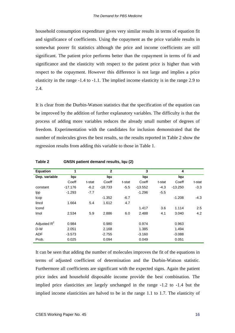
It is clear from the Durbin-Watson statistics that the specification of the equation can

be improved by the addition of further explanatory variables. The difficulty is that the

process of adding more variables reduces the already small number of degrees of

freedom. Experimentation with the candidates for inclusion demonstrated that the

number of molecules gives the best results, so the results reported in Table 2 show the

regression results from adding this variable to those in Table 1.


Equation 1 2 3 4



constant -17.176 -6.2 -18.733 -5.5 -13.552 -4.3 -13.250 -3.3

lpp -1.293 -7.7 -1.296 -5.5

lcop -1.352 -6.7 -1.208 -4.3

lincd 1.664 5.4 1.612 4.7

lcond 1.417 3.6 1.114 2.5

lmol 2.534 5.9 2.886 6.0 2.488 4.1 3.040 4.2

Adjusted R2 0.984 0.980 0.974 0.963

D-W 2.051 2.168 1.385 1.494

ADF -3.573 -2.755 -3.160 -3.088

Prob. 0.025 0.094 0.049 0.051

It can be seen that adding the number of molecules improves the fit of the equations in

terms of adjusted coefficient of determination and the Durbin-Watson statistic.

Furthermore all coefficients are significant with the expected signs. Again the patient

price index and household disposable income provide the best combination. The

implied price elasticities are largely unchanged in the range -1.2 to -1.4 but the

implied income elasticities are halved to be in the range 1.1 to 1.7. The elasticity of



demand with respect to the number of medicines available demonstrates the largest

effect ranging from 2.5 to 3.0.

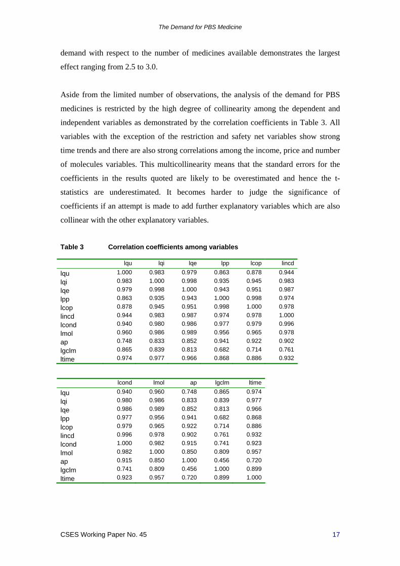
Aside from the limited number of observations, the analysis of the demand for PBS

medicines is restricted by the high degree of collinearity among the dependent and

independent variables as demonstrated by the correlation coefficients in Table 3. All

variables with the exception of the restriction and safety net variables show strong

time trends and there are also strong correlations among the income, price and number

of molecules variables. This multicollinearity means that the standard errors for the

coefficients in the results quoted are likely to be overestimated and hence the t-

statistics are underestimated. It becomes harder to judge the significance of

coefficients if an attempt is made to add further explanatory variables which are also

collinear with the other explanatory variables.

Table 3 Correlation coefficients among variables

lqu lqi lqe lpp lcop lincd

lqu 1.000 0.983 0.979 0.863 0.878 0.944

lqi 0.983 1.000 0.998 0.935 0.945 0.983

lqe 0.979 0.998 1.000 0.943 0.951 0.987

lpp 0.863 0.935 0.943 1.000 0.998 0.974

lcop 0.878 0.945 0.951 0.998 1.000 0.978

lincd 0.944 0.983 0.987 0.974 0.978 1.000

lcond 0.940 0.980 0.986 0.977 0.979 0.996

lmol 0.960 0.986 0.989 0.956 0.965 0.978

ap 0.748 0.833 0.852 0.941 0.922 0.902

lgclm 0.865 0.839 0.813 0.682 0.714 0.761

ltime 0.974 0.977 0.966 0.868 0.886 0.932

lcond lmol ap lgclm ltime

lqu 0.940 0.960 0.748 0.865 0.974

lqi 0.980 0.986 0.833 0.839 0.977

lqe 0.986 0.989 0.852 0.813 0.966

lpp 0.977 0.956 0.941 0.682 0.868

lcop 0.979 0.965 0.922 0.714 0.886

lincd 0.996 0.978 0.902 0.761 0.932

lcond 1.000 0.982 0.915 0.741 0.923

lmol 0.982 1.000 0.850 0.809 0.957

ap 0.915 0.850 1.000 0.456 0.720

lgclm 0.741 0.809 0.456 1.000 0.899

ltime 0.923 0.957 0.720 0.899 1.000



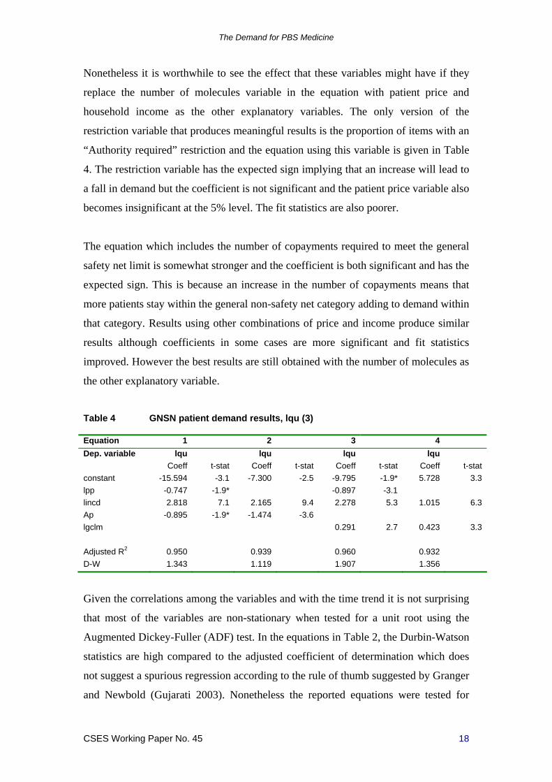
Nonetheless it is worthwhile to see the effect that these variables might have if they

replace the number of molecules variable in the equation with patient price and

household income as the other explanatory variables. The only version of the

restriction variable that produces meaningful results is the proportion of items with an

“Authority required” restriction and the equation using this variable is given in Table

4. The restriction variable has the expected sign implying that an increase will lead to

a fall in demand but the coefficient is not significant and the patient price variable also

becomes insignificant at the 5% level. The fit statistics are also poorer.

The equation which includes the number of copayments required to meet the general

safety net limit is somewhat stronger and the coefficient is both significant and has the

expected sign. This is because an increase in the number of copayments means that

more patients stay within the general non-safety net category adding to demand within

that category. Results using other combinations of price and income produce similar

results although coefficients in some cases are more significant and fit statistics

improved. However the best results are still obtained with the number of molecules as

the other explanatory variable.


Equation 1 2 3 4



constant -15.594 -3.1 -7.300 -2.5 -9.795 -1.9* 5.728 3.3

lpp -0.747 -1.9* -0.897 -3.1

lincd 2.818 7.1 2.165 9.4 2.278 5.3 1.015 6.3

Ap -0.895 -1.9* -1.474 -3.6

lgclm 0.291 2.7 0.423 3.3

Adjusted R2 0.950 0.939 0.960 0.932

D-W 1.343 1.119 1.907 1.356

Given the correlations among the variables and with the time trend it is not surprising

that most of the variables are non-stationary when tested for a unit root using the

Augmented Dickey-Fuller (ADF) test. In the equations in Table 2, the Durbin-Watson

statistics are high compared to the adjusted coefficient of determination which does

not suggest a spurious regression according to the rule of thumb suggested by Granger

and Newbold (Gujarati 2003). Nonetheless the reported equations were tested for



cointegration by testing their residuals for stationarity again using the ADF test (as

suggested by Gujarati). Cointegration means that the equation represents a valid long-

run relationship among the variables and this is demonstrated by the ADF test

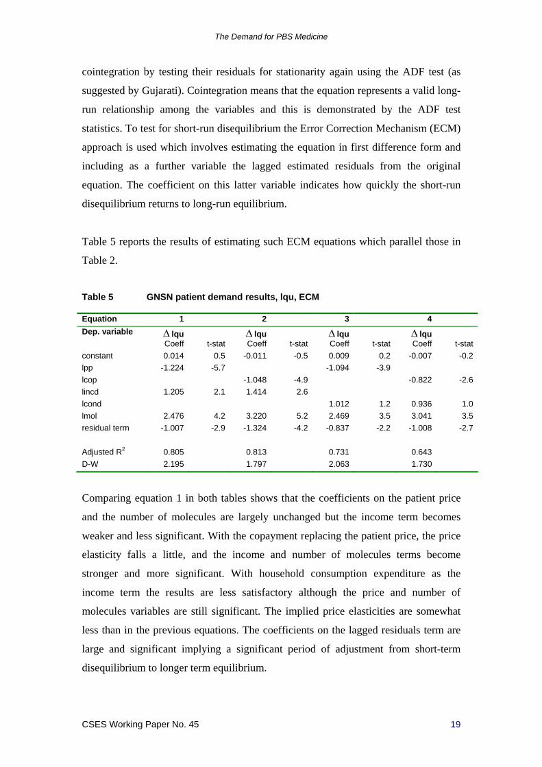
statistics. To test for short-run disequilibrium the Error Correction Mechanism (ECM)

approach is used which involves estimating the equation in first difference form and

including as a further variable the lagged estimated residuals from the original

equation. The coefficient on this latter variable indicates how quickly the short-run

disequilibrium returns to long-run equilibrium.

Table 5 reports the results of estimating such ECM equations which parallel those in

Table 2.

Table 5 GNSN patient demand results, lqu, ECM

Equation 1 2 3 4



constant 0.014 0.5 -0.011 -0.5 0.009 0.2 -0.007 -0.2

lpp -1.224 -5.7 -1.094 -3.9

lcop -1.048 -4.9 -0.822 -2.6

lincd 1.205 2.1 1.414 2.6

lcond 1.012 1.2 0.936 1.0

lmol 2.476 4.2 3.220 5.2 2.469 3.5 3.041 3.5

residual term -1.007 -2.9 -1.324 -4.2 -0.837 -2.2 -1.008 -2.7

Adjusted R2 0.805 0.813 0.731 0.643

D-W 2.195 1.797 2.063 1.730

Comparing equation 1 in both tables shows that the coefficients on the patient price

and the number of molecules are largely unchanged but the income term becomes

weaker and less significant. With the copayment replacing the patient price, the price

elasticity falls a little, and the income and number of molecules terms become

stronger and more significant. With household consumption expenditure as the

income term the results are less satisfactory although the price and number of

molecules variables are still significant. The implied price elasticities are somewhat

less than in the previous equations. The coefficients on the lagged residuals term are

large and significant implying a significant period of adjustment from short-term

disequilibrium to longer term equilibrium.



If the quantity index is used as the dependent variable rather than the number of units,

the results are broadly similar to those just reported in terms of both fit statistics and

coefficients on variables. The price, income and number of molecules variables are

significant with the expected signs on the coefficients. The implied price elasticities

are somewhat less but closer together in the range -1.2 to -1.0. Both the elasticities

with respect to income and the number of molecules are significantly higher being in

the range from 1.8 to 2.7 and 3.5 to 4.0 respectively. The larger elasticities when the

quantity index is used as the dependent variable rather than the number of units may

indicate that the elasticities are expressing both a quantity and a “quality” component

in the response of patients to changes in the explanatory variables. Table 6 reports the

preferred equation and its ECM equivalent

Table 6 GNSN patient demand results, lqi

Equation 1 2

Dep. variable lqi lqi

Coeff t-stat Coeff t-stat

constant -55.573 -10.9 0.091 2.6

lpp -1.143 -3.7 -1.096 -4.1

lincd 2.683 4.7 0.866 1.2

lmol 3.480 4.4 1.722 1.9

residual term -0.740 -2.7

Adjusted R2 0.988 0.604

D-W 2.050 2.019

ADF -4.391

Prob 0.005

The ADF test on the residuals of the equation indicates a cointegrating relationship

but the coefficients on the income and number of molecules variables in the ECM

equation lose significance with the main explanation for short-run disequilibrium

being the change in prices. Although not reported, substituting either the restriction or

the safety net limit variable for the number of molecules gives significant coefficients

of the expected sign for these variables but in combination with the price variables

produces insignificant coefficients for the latter. Again the best results come from

using the number of molecules variable with the price and income variables.

If the deflated PBS expenditure series is used as the quantity measure for the

dependent variable, the difference in regression outcomes is enhanced. The



coefficients on the income and number of molecules variables increase further

although the price elasticities remain with a range of -1.2 to -1.3. The ADF tests

indicate the variables are cointegrated and the ECM equations show significant

coefficients on the price and number of molecules variables but the income term is not

significant. The preferred equation and its ECM equivalent are given in Table 7. As

the dependent variable includes net new items in addition to the common items as

well as the possible “quality” component this may explain the greater response of

patients as measured by the higher elasticities for income and the number of

molecules.

Table 7 GNSN patient demand results, lqe

Equation 1 2

Dep. variable lqe lqe

Coeff t-stat Coeff t-stat

constant -67.370 -13.4 0.107 3.6

lpp -1.208 -3.9 -1.322 -5.3

lincd 3.240 5.8 1.004 1.5

lmol 4.235 5.4 2.574 3.5

residual term -0.768 -3.4

Adjusted R2 0.993 0.730

D-W 1.987 2.636

ADF -3.572

Prob 0.022

To this point, regression results have been reported for aggregate analysis based on 15

annual observations. An alternative approach using quantity and price data for each

PBS item within the dataset can be used to estimate the demand equation for each

patient category. Here a quasi-panel approach is adopted with the dependent variable

being the number of units of item i in year t and the equation specified as follows

1 1

R Kr k

it it t t it it itr k

q p M c RES ATC u

(1.11)

In contrast to the aggregate approach there is only one measure of quantity and that is

the number of units for the item in a specific year, measured as the number of scripts

times the average maximum quantity. This is the same quantity measure used in

deriving the price and quantity indexes. Two price variables are considered. The first

is the patient price derived by dividing the patient cost by the quantity measure and



again this is the raw data used in the calculation of the price and quantity indexes. The

second price considered is the average copayment for the year and is hence the same

for all items in that year. As previously, two income variables are considered –

household disposable income and household consumption expenditure – and these are

also the same for each item in a particular year. The c variable represents the number

of copayments required to reach the safety net limit which varies by year but not by

item. A set of dummy variables are used to account for the restriction status (RES) of

the item and another set of dummy variables are used to control for the ATC code of

the item. The values of both of these dummy variables can vary among items and

from year to year. As with the equations at the aggregate level, only results for the

logarithmic version are reported as these are generally superior to those using

untransformed variables.

The dataset for the regression analysis is formed by “stacking” the block of

observations for one year on top of the following year. Data is therefore ordered first

by item then by year. The data is not a complete panel because there are not

observations for all items in all years. However it is possible to organize the data as a

balanced panel within the EViews software package (Quantitative Micro Software

2007) with the missing observations acknowledged as such and ignored in the

analysis. Organising the data in this way has the advantage of enabling time-ordered

diagnostics to be computed even though the regression analysis is based just on OLS

without any panel effects being specified. These are accounted for in part by the

dummy variables.

Table 8 reports the results of estimating equation (1.11) with the patient price as the

price variable and household income as the income variable.

Substituting the copayment and household consumption expenditure produces similar

results although the overall fit is worse. The only difference among equations 1-5 in

Table 8 is that the ATC code dummy variables are defined at successively higher

ATC levels beginning with no ATC dummy variables, then those defined at ATC1,

ATC3, ATC4 and ATC5 levels.



It is obvious from Table 8 that as the ATC codes become more specific to the actual

item the fit of the equations improves considerably at least when measured by the

adjusted R2. The coefficient on the patient price variable is relatively unchanged and

is in the range -1.4 to -1.2. However the coefficient on the income variable reduces

with higher levels of ATC code and becomes insignificant at the ATC5 level. The

coefficient of the number of copayments to reach the general safety net limit is

significant and has the expected sign but also reduces as ATC level increases. The

only restriction variable that has any impact is the dummy variable for “Authority

required” or not and while significant has an unexpected positive sign except at ATC5

when the sign becomes negative.

Table 8 GNSN patient demand results, item level data, n=18005

Equation 1 2 3 4



constant -17.413 -6.4 -14.641 -5.6 -10.604 -4.3 -8.217 -3.4

lpp -1.363 -103.4 -1.251 -84.3 -1.218 -76.7 -1.233 -74.8

lincd 1.783 7.1 1.464 6.1 0.963 4.3 0.830 3.8

lgclm 1.057 4.9 1.085 5.3 0.887 4.6 0.684 3.8

A 0.513 9.3 0.706 13.2 0.625 11.1 0.359 6.2

ATC level ATC1 ATC3 ATC4

Adjusted R2 0.381 0.437 0.511 0.560

D-W 0.115 0.127 0.147 0.166

Equation 5 6 7

Dep. variable lqu lqu lqu

Coeff t-stat Coeff t-stat Coeff t-stat

constant 3.592 1.3 2.675 1.6 -1.133 -0.6

lpp -1.274 -73.7 -1.275 -74.7

lcop -1.614 -10.5

lincd -0.085 -0.4

lgclm 0.519 3.2 0.468 4.1 0.570 3.2

A -0.460 -6.9 -0.460 -6.9 -0.457 -6.0

ATC level ATC5 ATC5 ATC5

Adjusted R2 0.644 0.644 0.535

D-W 0.201 0.201 0.156

Pedroni test 11/11 9/11 9/11

Omitting the income variable gives equation 6 as the preferred equation in Table 8

and the Pedroni Residual Cointegration Test within EViews indicates that the



variables (excluding the ATC dummy variables) for this equation are cointegrated.

Table 8 also shows the results if the copayment is substituted for the patient price. In

this latter case, although all variables have significant coefficients, the overall fit of

the equation has diminished.

The demand elasticities of the patient price and the copayment implied by these

equations are close to those values derived from the aggregate equations.

4.2 Results for Concessional Non-Safety Net (CNSN) patients

When equations are estimated explaining the demand for PBS medicines by

Concessional Non-Safety Net (CNSN) patients with (the logarithm of) the number of

units as the dependent variable, the outcomes are similar to those for General Non-

Safety Net patients in that the price and income variables are significant and the fit

statistics quite similar. The number of molecules variable is significant when

household disposable income is the income variable but not for household

consumption expenditure. However the implied price elasticities are less than half

those for GNSN patients and are in a much tighter range from -0.43 to -0.47.

Similarly the income elasticities are almost half those for GNSN patients in the range

0.64 to 0.90. The elasticity for the number of molecules ranges between 0.53 and

0.73. The ADF test statistics indicate cointegrating relationships among the variables

and the corresponding short-term ECM equations give broadly similar results

although those including household consumption expenditure perform poorly.

Replacing the number of molecules by the restriction variable leads to poorer results

although the variable itself has a significant coefficient of the expected sign when the

income variable is household consumption expenditure. Similarly the number of

copayments to reach the safety net limit performs poorly as an explanatory variable.

Equation 1 in Table 9 reports the preferred equation with patient price, household

disposable income and number of molecules as explanatory variables.

If the quantity index or deflated PBS expenditure is used as the dependent variable the

results again mirror the experience with GNSN patients. There is an improvement in

fit statistics and an increase in the values of the coefficients on the price, income and

number of molecules variables. With the quantity index equations the price and



income elasticity ranges are -0.76 to -0.86 and 2.11 to 2.41 respectively while the

range for the elasticity for the number of molecules increases dramatically to 2.41 to

2.87. With deflated PBS expenditure as the dependent variable the ranges are even

higher at -0.73 to -0.94 for the price elasticity and 2.63 to 2.77 and 2.48 to 3.24 for the

income and number of molecules elasticities. The preferred equations for both

variants of the demand equation are given as equations 2 and 3 in Table 9.

Table 9 CNSN patient demand results

Equation 1 2 3

Dependent variable lqu lqi lqe


constant 7.184 6.1 -47.184 -15.7 -53.375 -13.5

lpp -0.439 -6.2 -0.756 -4.2 -0.731 -3.1

lincd 0.895 6.3 2.404 6.6 2.717 5.7

lmol 0.533 2.6 2.698 5.2 3.053 4.5

Adjusted R2 0.981 0.994 0.993

D-W 1.122 2.001 1.100

ADF -5.543 -4.312 -2.697

Prob. 0.006 0.007 0.105

Using the detailed data on units and prices for CNSN patients, the demand equations

results are somewhat different from those for GNSN patients. While the patient price

is strongly significant, the copayment performs poorly as the price variable. The

income variable is significant at all ATC levels including ATC5 but the number of

concessional copayments to reach the safety net limit is always insignificant. By

contrast, including dummy variables for the “Authority required” and Restricted

Benefit” restriction classifications produces strongly significant coefficients with the

expected signs at all ATC levels and the effect is much stronger for the “A” items

than for the “R” items. In general the fit off the equation improves as the ATC level

increases. The implied price elasticity for the preferred equation at the ATC5 level is -

1.39 and this is significantly higher than suggested by the aggregate equations but

very close to that for GNSN patients (Table 10).



Table 10 CNSN patient demand results, item level data, n=23612

Dependent variable lqu

Coeff t-stat

constant -24.476 -2.0

lpp -1.395 -95.6

lincd 1.223 8.2

lcclm 4.038 1.2

A -1.877 -27.2

R -0.622 -11.5

ATC level ATC5

Adjusted R2 0.627

D-W 0.099

Pedroni tests 9/11

4.3 Results for General Safety Net (GSN) patients

While the regression analyses of the demand for PBS medicines by patients within the

general and concessional non-safety net categories produce robust results and

significant estimates for elasticities, the results for patients within the two safety net

categories are much weaker.

For General Safety Net (GSN) patients the only significant variables are income and

the copayment limit in equations estimated using aggregate data. Patient price,

copayment, the number of molecules and restriction levels all produce insignificant

coefficients. The best regression result is shown as equation 1 in Table 11 with the

household disposable income and the number of copayments to reach the general

safety net limit as explanatory variables, with the latter variable lagged by one year.

The fit statistics of the equation is much poorer than those for the previous two patient

categories. The income elasticity is in the range 1.15 to 1.38 and the coefficient on the

lagged copayment limit is significant and has the expected sign, indicating a reduced

demand when the copayment is increased as more patients remain within the general

non-safety net category. The ADF tests indicate a cointegrating relationship.



Table 11 GSN patient demand results

Equation 1 2 2



constant 4.398 1.1 -40.852 -10.0 -45.615 -10.8

lincd 1.377 3.6 3.461 9.3 3.846 10.1

lgclm(-1) -0.907 -3.2 -0.698 -2.5 -0.731 -2.6

Adjusted R2 0.475 0.911 0.924

D-W 2.462 2.481 2.473

ADF -4.385 -4.493 -4.455

Prob. 0.006 0.005 0.005

The equations with the quantity index and deflated PBS expenditure as dependent

variables show similar outcomes although there is a big jump in the fit statistics

(equations 2 and 3 in Tables 11). As with the other patient categories the coefficient

on the income variable increases markedly and the coefficient on the copayment limit

becomes somewhat smaller in absolute terms.

Using item level data for quantity and price, the results are quite different. In this

circumstance all the variables are significant and have their expected signs at all ATC

levels. The preferred equation given in Table 12 which includes ATC5 dummy

variables has an implied patient price elasticity of -1.37 and this is very close to that

for the same equation for CNSN patients.

Table 12 GSN patient demand results, item level data, n=21470


Coeff t-stat

constant -16.463 -8.0

lpp -1.371 -105.0

lincd 1.722 11.0

lgclm -0.706 -5.4

A -1.428 -23.2

R -0.457 -9.6

ATC level ATC5

Adjusted R2 0.659

D-W 0.188

Pedroni tests 9/11

It should be remembered that GSN and CNSN patients both pay the same

concessional copayment so the patient price series in both cases will be very similar.



The income coefficient is also significant at ATC5 level although somewhat higher in

value than for CNSN patients. Both the “A” and “R” restriction dummy variables are

significant, have the expected signs and the same sort of disparity in value. For GSN

patients however the number of copayments to reach the safety net limit is significant

and negative. This is the mirror of the positive coefficient for GNSN patients. Again

like the GNSN patients, replacing the patient price by the copayment gives significant

results although poorer overall fit. It makes very little difference if household

consumption expenditure is used as the income variable.

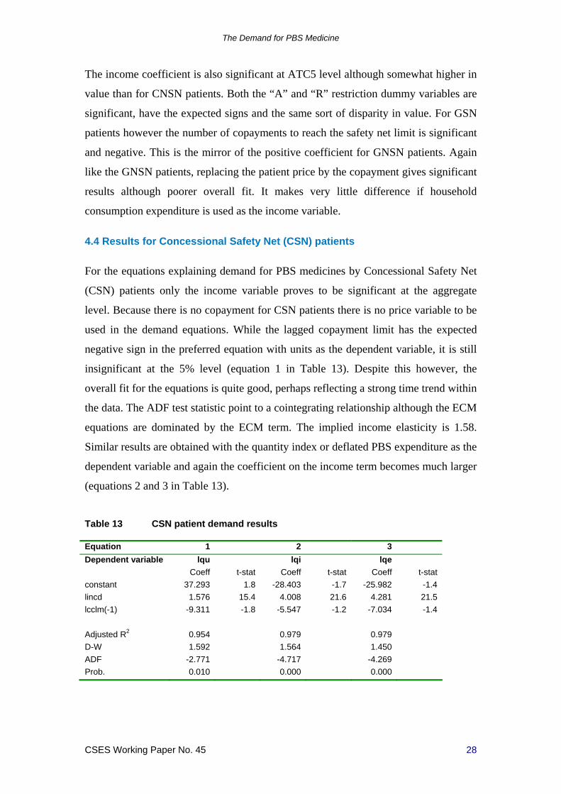
4.4 Results for Concessional Safety Net (CSN) patients

For the equations explaining demand for PBS medicines by Concessional Safety Net

(CSN) patients only the income variable proves to be significant at the aggregate

level. Because there is no copayment for CSN patients there is no price variable to be

used in the demand equations. While the lagged copayment limit has the expected

negative sign in the preferred equation with units as the dependent variable, it is still

insignificant at the 5% level (equation 1 in Table 13). Despite this however, the

overall fit for the equations is quite good, perhaps reflecting a strong time trend within

the data. The ADF test statistic point to a cointegrating relationship although the ECM

equations are dominated by the ECM term. The implied income elasticity is 1.58.

Similar results are obtained with the quantity index or deflated PBS expenditure as the

dependent variable and again the coefficient on the income term becomes much larger

(equations 2 and 3 in Table 13).

Table 13 CSN patient demand results

Equation 1 2 3



constant 37.293 1.8 -28.403 -1.7 -25.982 -1.4

lincd 1.576 15.4 4.008 21.6 4.281 21.5

lcclm(-1) -9.311 -1.8 -5.547 -1.2 -7.034 -1.4

Adjusted R2 0.954 0.979 0.979

D-W 1.592 1.564 1.450

ADF -2.771 -4.717 -4.269

Prob. 0.010 0.000 0.000



For equations using data defined at the item level, the regression results show no

significance for either the income term or for the copayment limit term although both

have the expected signs (Table 14). The only significant explanatory variables are the

“A” and “R” restriction dummy variables and again they have the expected sign and

the disparity between their coefficients is the same as that seen for both GSN and

CNSN patients.

Table 14 CSN patient demand results, item level data, n=22248


Coeff t-stat

constant 12.492 0.9

lincd 0.182 1.0

lcclm -2.767 -0.7

A -1.523 -18.7

R -0.379 -5.9

ATC level ATC5

Adjusted R2 0.496

D-W 0.101

Pedroni tests 10/11

5 Summary of econometric analysis

The results quoted in the previous section show that the demand for PBS medicines is

significantly influenced by two of the policy instruments controlled by the

Government. On the one hand demand increases more than proportionately to the

steadily increasing number of medicines made available through the operation of the

PBS listing procedures. As the PBAC makes available more choice among medicines

to treat particular diseases and introduces medicines for diseases previously untreated

or poorly treated, doctors prescribe these for their patients reducing the burden of

disease. On the other hand demand is reduced when Governments increase the amount

patients are required to pay for these medicines and to a lesser extent when

manufacturers change the premium they add to the base dispensed price.

For General Non-Safety Net (GNSN) patients the patient price elasticity is in the

range -1.1 to -1.4, while for Concessional Non-Safety Net (CNSN) patients it is

significantly lower in the range -0.5 to -0.9. The situation is less clear with General



Safety Net (GSN) patients although analysis using detailed data suggests an elasticity

of -1.4. The demand elasticities with respect to either the patient price or the

copayment are significantly higher than those found in previous studies of the demand

for PBS medicines. They are however similar to recent estimates made by Berndt,

Danzon and Kruse (2007) who report own-price elasticities in the range -0.75 to -1.1

based on an analysis using IMS health data from 1992 to 2003 across 15 countries,

not including Australia.

The income elasticity is generally significant but there is more variability in the

estimates depending on how the dependent variable is defined and at what level the

analysis is undertaken. The elasticity is higher if the quality-adjusted quantity

variables are used rather than the number of units for all categories of patients. The

elasticity with respect to the number of molecules also shows the same tendency to

increase. For most of the regression analyses the elasticities with respect to income

and the number of molecules is significantly higher than one. The estimates show

significant contributions to the demand for PBS medicines from rising incomes and as

the number of medicines available on the PBS increases.

There is further evidence that when the Government imposes an “Authority required”

restriction level on a PBS item this restricts demand for that item. Other restriction

levels seem not to have this effect.

The level of the copayment set by the Government has the dual effect of both

reducing demand because of its price effect and of shifting the share of the cost to the

patient and away from the Government. Changes to the safety net limit however shift

demand within a patient category between those covered by the safety net and those

not covered. Increases in the safety net limit reduce demand within the safety net

category and again lead to shifts in the shares of cost borne by patients and the

Government.

While these effects are generally true for all PBS patients, there are significant

differences among the patient categories. General patients display a greater reaction to

changes in the patient price than do concessional patients. One explanation for this

may lie in the types of medicines consumed by both groups. If concessional patients

have a higher proportion of chronic conditions or conditions displaying symptoms



then changes in prices may have less influence on their purchasing decisions. If

general patients have more acute conditions or asymptotic conditions they may be

more influenced by changes in prices. It should be remembered however that the

concessional copayment is less than a sixth the value of the general copayment and

this may not be fully accounted for in the regression results. The difference in

conditions experienced by general and concessional patients may also explain their

differential responses to the number of molecules and income.

The demand by general patients also seems to be more sensitive to changes in the

safety net limit than is the demand by concessional patients. This may simply reflect

the fact that the safety net limit for concessional patients changed very little for most

of the period.

For both general and concessional patients, the responsiveness of patients to changes

in the explanatory variables as measured by the elasticities increase when different

measures of quantity are used. Moving from the number of units to the quantity index

may be adding a “quality” factor to the quantity measure and the responsiveness of

patient could be due to this. With the deflated expenditure as quantity measure, the

influence of net new items is also incorporated again with a further response from

patients.

Estimating equations using price and quantity data defined at the aggregate level

clearly demonstrates the importance of the number of molecules listed on the PBS,

while using data defined at the detailed item level enables the influence of both

restriction levels and safety net limits to be better understood.



6 References

Barten A P 1964, Consumer Demand Functions Under Conditions of Almost Additive

Preferences’, Econometrica, Vol 32, No 1-2, January-April 1964, 1-38

Berndt, Ernst R, Ashoke Battacharjya, David N Mishol, Almudena Arcelus, and

Thomas Lasky 2002, ‘An Analysis of the Diffusion of New Antidepressants: Variety,

Quality, and Marketing Efforts’, The Journal of Mental Health Policy and Economics,

5, 3-19

Berndt Ernst R, Linda Bui, David Lucking-Reiley, and Glen Urban 1994, ‘The Roles

of Marketing, Product Quality, and Price Competition in the Growth and Composition

of the US Antiulcer Drug Industry’, Chapter 7 of Timothy F Bresnahan and Robert J

Gordon (ed) 1997

Berndt Ernst R, Patricia M Danzon and Gregory B Kruse 2007, ‘Dynamic

Competition in Pharmaceuticals: Cross-National Evidence from New Drug

Diffusion’, Managerial and Decision Economics, 2007, 28, 231–250

Berndt, Ernst R, Robert S Pindyck and Pierre Azoulay 1999, ‘Consumption

Externalities and Diffusion in Pharmaceutical Markets: Antiulcer Drugs’, The Journal

of Industrial Economics, Volume LI, June 2003, No 2 , 243-270

Bureau of Industry Economics 1985, Retail pharmacy in Australia – an economic

appraisal, Research report 17, Australian Government Publishing Service, Canberra,

1985

Cleanthous Paris 2004, ‘Welfare Implications of U.S. Antidepressant Innovation’,

New York University, October 2004



Clements Kenneth W, Antony Selvanathan and Saroja Selvanathan 1996, ‘Applied

Demand Analysis: A Survey’, The Economic Record, Vol 72, No 216, March 1996,

63-81

Cockburn Iain M and Aslam H Anis 2001, ‘Hedonic Analysis of Arthritic Drugs’,

Chapter 11 of Cutler David M and Ernst R Berndt (eds) 2001

Cutler, David M and Ernst R Berndt (eds) 2001, Medical Care Output and

Productivity, The University of Chicago Press, Chicago, 2001

Deaton Angus and John Muellbauer 1980a, Economics and consumer behavior,

Cambridge University Press, Cambridge, UK, 1980

Deaton Angus and John Muellbauer 1980b, ‘An Almost Ideal Demand System’,

American Economic Review, Vol 70, No 3, June 1980, 312-326

Department of Health and Aged Care 2000, National Medicines Policy 2000,

Department of Health and Aged Care, Canberra, 1999 at

http://www.health.gov.au/internet/wcms/publishing.nsf/Content/nmp-objectives-

policy.htm

Department of Health and Ageing 2005, New PBS Safety Net thresholds, Department

of Health and Ageing, Canberra, December 2005 at

http://www.health.gov.au/internet/main/publishing.nsf/Content/pbs-safetynet-changes

Department of Health and Ageing 2007a, Australian Statistics on Medicine 2004-

2005, Commonwealth of Australia, 2007, available at

http://www.pbs.gov.au/html/healthpro/publication/list

Department of Health and Ageing 2007j Schedule of Pharmaceutical Benefits for

Approved Pharmacists and Medical Practitioners, Commonwealth of Australia,

Canberra, various issues, available at

http://www.pbs.gov.au/html/healthpro/publication/list



Donohue Julie M and Ernst R Berndt 2004, ‘Effects of Direct-to-Consumer

Advertising on Medication Choice: The Case of Antidepressants’, Journal of Public

Policy and Marketing, Vol 23 (2), Fall 2004, 115-127

Ellison Sarah Fisher and Judith K Hellerstein 1999, ‘The Economics of Antibiotics:

An Exploratory Study’, in Triplett Jack E (ed) 1999

Harvey Roy 1984, ‘The Effect of Variations in Patient Contribution, Income, and

Doctor Supply on the Demand for PBS Drugs’, in Tatchell P M (ed) 1984, Economics

and health 1983, Proceedings of the fifth Australian Conference of Health

Economists, Technical Paper 8, Health Economics Research Unit, Australian National

University, Canberra, 1984

Johnston Mark 1990, ‘The Price Elasticity of Demand for Pharmaceuticals’, in Selby

Smith C (ed) 1991, Economics and Health: 1990, Proceedings of the Twelfth

Australian Conference of Health Economists, Public Sector Management Institute,

Monash University, Melbourne, 1991

McManus, Peter, Neil Donnelly, David Henry, Wayne Hall, John Primrose and Julie

Lindner 1996, ‘Prescription Drug Utilization Following Patient Co-Payment Changes

in Australia’, Pharmacoepidemiology and Drug Safety, Vol 5, 1996, 385-392

Parliamentary Library 2005, Bills Digest no. 56 2005–06, National Health

Amendment (Budget Measures—Pharmaceutical Benefits Safety Net) Bill 2005,

Parliament of Australia, Canberra, October 2005 at

http://www.aph.gov.au/library/Pubs/bd/2005-06/06bd056.htm

Quantitative Micro Software 2007, EViews 6 User’s Guides I and II, Quantitative

Micro Software LLC, Irvine, California, January 9 2007

Reserve Bank of Australia 2007c, Gross Domestic Product – Income Components,

Bulletin Statistical Table G12, RBA, at

http://www.rba.gov.au/Statistics/Bulletin/index.html



Rosenthal Meredith B, Ernst R Berndt, Julie M Donohue, Arnold M Epstein and

Richard G Frank 2003, Demand Effects of Recent Changes in Prescription Drug

Promotion, Kaiser Family Foundation, June 2003 at http://www.kff.org/rxdrugs/6085-

index.cfm

Stone Richard 1954, “Linear Expenditure Systems and Demand Analysis; An

Application to the Pattern of British Demand’, Economic Journal, 64, 511-527

Suslow Valerie Y 1996, ‘Measuring Quality Change in the Market for Anti-Ulcer

Drugs’, in Helms Robert E (ed) 1996

Theil H 1975, Theory and Measurement of Consumer Demand, North-Holland,

Amsterdam



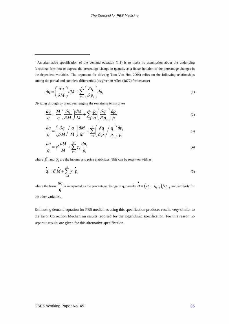
i An alternative specification of the demand equation (1.1) is to make no assumption about the underlying

functional form but to express the percentage change in quantity as a linear function of the percentage changes in

the dependent variables. The argument for this (eg Tran Van Hoa 2004) relies on the following relationships

among the partial and complete differentials (as given in Allen (1972) for instance)

1

n

ii i

q qdq dM dp

M p

(1)

Dividing through by q and rearranging the remaining terms gives

1

ni i

i ii

p dpdq M q dM q

q q M M q p p

(2)

1

ni

i i i i

dpdq dMq q q qM M p pq M p

(3)

1

ni

ii i

dpdq dM

q M p

(4)

where and i are the income and price elasticities. This can be rewritten with as

1

n

i ii

q M p

(5)

where the form dq

qis interpreted as the percentage change in q, namely 1 1t t tq q q q

and similarly for

the other variables.

Estimating demand equation for PBS medicines using this specification produces results very similar to

the Error Correction Mechanism results reported for the logarithmic specification. For this reason no

separate results are given for this alternative specification.

Documents

The Demand for PBS Medicine - Victoria Universityvuir.vu.edu.au/15935/1/15935.pdf · The Demand for PBS Medicine ... including the fact that the income elasticity for necessities