The demand for a healthy diet: estimating the almost ideal demand system with infrequency of purchase Article 

Accepted Version 

Tiffin, R. and Arnoult, M. (2010) The demand for a healthy diet: estimating the almost ideal demand system with infrequency of purchase. European Review of Agricultural Economics, 37 (4). pp. 501­521. ISSN 0165­1587 doi: https://doi.org/10.1093/erae/jbq038 Available at http://centaur.reading.ac.uk/16773/ 

It is advisable to refer to the publisher’s version if you intend to cite from the work. 

To link to this article DOI: http://dx.doi.org/10.1093/erae/jbq038 

Publisher: Oxford University Press 

All outputs in CentAUR are protected by Intellectual Property Rights law, including copyright law. Copyright and IPR is retained by the creators or other copyright holders. Terms and conditions for use of this material are defined in the End User Agreement  . 

www.reading.ac.uk/centaur   

CentAUR 

Central Archive at the University of Reading 

Reading’s research outputs online

1

The demand for a healthy diet: estimating the almost ideal

demand system with infrequency of purchase.

Richard Tiffin1

Department of Food Economics and Marketing, University of Reading, UK

Matthieu Arnoult

Land Economy and Environment, Scottish Agricultural College, Edinburgh, UK.

Summary

A Bayesian method of estimating multivariate sample selection models is introduced and applied to

the estimation of a demand system for food in the UK to account for censoring arising from

infrequency of purchase. We show how it is possible to impose identifying restrictions on the

sample selection equations and that, unlike a maximum likelihood framework, the imposition of

adding up at both latent and observed levels is straightforward. Our results emphasise the role

played by low incomes and socio-economic circumstances in leading to poor diets and also indicate

that the presence of children in a household has a negative impact on dietary quality.

Keywords: Almost Ideal Demand System, Censoring, Bayesian Estimation, Diet and Health.

JEL classification: C11, C24, D12

1 Introduction

It is increasingly recognised that diet related chronic disease represents one of the most significant

public health challenges of the twenty-first century. For example the prevalence of overweight and

obesity has grown rapidly since the 1980s and, according to the Health Survey for England, in 2008

66% of the adult males and 57% of adult females had a BMI greater than 25 while 25% of adult

males and 24% of adult females were obese (BMI greater than 30). In addition to obesity, the roles

that can be played by fruit and vegetables in the prevention of cancer also commands attention as do

the impacts of dietary fat composition on fat and lipoprotein levels in the blood and associated

impacts on heart disease. There is also a recognition (Drewnowski, 2004, Dowler, 2003) that diet

related health problems are not evenly distributed in society. The first objective of this paper is

therefore to apply an economic framework to analyse the factors which contribute to this uneven

distribution. To do this we estimate a demand model which incorporates socio-demographic

variables using micro-data.

Micro-data are in general subject to the econometric problem of censoring. In demand analysis this

arises because most households do not purchase all of the commodities available to them. Wales

and Woodland (1983) introduce two econometric models for censored demand systems. They refer

to the first model as the Kuhn-Tucker approach. As its name implies, it is based on the Kuhn-Tucker

conditions for the consumer‟s optimisation problem. The econometric model is developed by

adding a stochastic term to the utility function and as a result to the Kuhn-Tucker conditions. The

conditions hold as an equality when an interior solution results and as an inequality when there is a

corner solution. As a result the likelihood function is of a mixed discrete-continuous form

(Pudney, 1989, p163) and is difficult to maximise for all but relatively small demand systems

because of the numerical integration that is required in its evaluation. The intractability of the

likelihood function has led to very few examples of the empirical implementation of the Kuhn-

Tucker approach; one example is Phaneuf et al. (2000). By contrast, the second model proposed by

Wales and Woodland (1983), which they refer to as the Amemiya-Tobin approach, has been more

1 Address for correspondence: Professor Richard Tiffin, Department of Food Economics and Marketing, University of

Reading, PO Box 237, Reading, RG6 6AR UK. E-mail: j.r.tiffin@reading.ac.uk.

2

widespread in the literature. This second strategy for handling censoring is an application of the

Tobit model (Tobin, 1958) as extended by Amemiya (1974) to the estimation of a system of

equations. In this approach the demand model is derived without explicitly incorporating the non-

negativity conditions. Instead these are added to the estimated model by truncating the distribution

of the stochastic demand choices to allow for a discrete probability mass at zero.

A number of strategies have been adopted to the estimation of the Amemiya-Tobin model. The

direct estimation of the system by maximum likelihood has been problematic for reasons of

computational complexity. Earlier attempts at the estimation of the Amemiya-Tobin model are

therefore based on the two stage approach proposed by Heien and Wessells (1990) and developed

by Shonkwiler and Yen (1999), which is itself an application of the Heckman (1979) method. The

two step approach can be considered a generalisation of the Amemiya-Tobin approach because it

comprises two sets of equations: in addition to the censored equations, additional equations are used

to model the censoring and this allows the possibility of a difference between the models which

determine the censoring rule and the continuous observations. The generalisation of the Tobit model

in this way is discussed in the context of demand for a single good by Blundell and Meghir (1987)

who refer to the model in which the sample selection rule and the continuous variable models differ

as the double hurdle model, a model introduced originally by Cragg (1971). The double hurdle

model is adapted by Blundell and Meghir (1987) to form an infrequency of purchase model which

addresses the fact that within a truncated survey period, observed purchases may differ from actual

demand as stocks are either built up or run down. Yen et al. (2003) note that two step estimation is

consistent but inefficient and they return to maximum likelihood estimation of the original

Amemiya-Tobin model using simulated and quasi maximum likelihood methods. These methods

are generalised in Stewart and Yen (2004) and Yen (2005) in an analogous way to the generalisation

offered by the two step estimators referred to above to account for differences in the processes

determining selection and the continuous variable. They recognise that this generalisation is the

multivariate equivalent of that proposed by Cragg (1971). Their models are estimated by maximum

likelihood and are thus efficient.

The second objective of this paper is to contribute to this literature by applying Bayesian methods to

the estimation of multivariate sample selection models. We also extend the range of models that

have been estimated by maximum likelihood hitherto to the infrequency of purchase model and we

incorporate the Wales and Woodland (1983, p. 273) approach to the imposition of adding-up which,

as Pudney (1989, p157) notes, has been problematic in a maximum likelihood context.

2 Infrequency of Purchase in the AIDS model

The Infrequency of Purchase Model (IPM) is developed in order to accommodate the fact that

censoring occurs in the demand system because a particular good may not be purchased by a

household during the time that it is surveyed as it is consuming from stocks purchased in other time

periods. Our approach draws on Blundell and Meghir (1987) in order to adapt the Almost Ideal

Demand System (AIDS) to incorporate infrequency of purchase. The censoring rule that relates

latent consumption2 of the ith commodity by the hth household to observed purchases

ihq is

as follows:

*

1,

0 0

ihih

ih it

ih

qy

q

y

(1)

2 In this specification of the model we assume that latent consumption for all goods is non-zero. In other words we

assume that all censoring is the result of infrequency of purchase. Whilst allowing for both infrequency of purchase and

true corner solutions would be preferable, such an approach introduces an identification problem since the source of a

zero may be either a non-purchase, a corner solution or both.

3

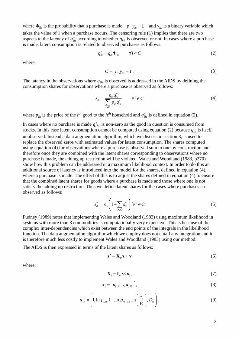
where Φih is the probability that a purchase is made 1ihp y and yih is a binary variable which

takes the value of 1 when a purchase occurs. The censoring rule (1) implies that there are two

aspects to the latency of according to whether is observed or not. In cases where a purchase

is made, latent consumption is related to observed purchases as follows:

*

ih ih ihq q i C (2)

where:

: 1 .ihC i y (3)

The latency in the observations where is observed is addressed in the AIDS by defining the

consumption shares for observations where a purchase is observed as follows:

*

*

ih ihih

ih ih

i C

p qs i C

p q (4)

where pih is the price of the ith good to the hth household and is defined in equation (2).

In cases where no purchase is made is non-zero as the good in question is consumed from

stocks. In this case latent consumption cannot be computed using equation (2) because qih is itself

unobserved. Instead a data augmentation algorithm, which we discuss in section 3, is used to

replace the observed zeros with estimated values for latent consumption. The shares computed

using equation (4) for observations where a purchase is observed sum to one by construction and

therefore once they are combined with the latent shares corresponding to observations where no

purchase is made, the adding up restriction will be violated. Wales and Woodland (1983, p270)

show how this problem can be addressed in a maximum likelihood context. In order to do this an

additional source of latency is introduced into the model for the shares, defined in equation (4),

where a purchase is made. The effect of this is to adjust the shares defined in equation (4) to ensure

that the combined latent shares for goods where a purchase is made and those where one is not

satisfy the adding up restriction. Thus we define latent shares for the cases where purchases are

observed as follows:

* *1 ih ih ih

i C

s s s i C (5)

Pudney (1989) notes that implementing Wales and Woodland (1983) using maximum likelihood in

systems with more than 3 commodities is computationally very expensive. This is because of the

complex inter-dependencies which exist between the end points of the integrals in the likelihood

function. The data augmentation algorithm which we employ does not entail any integration and it

is therefore much less costly to implement Wales and Woodland (1983) using our method.

The AIDS is then expressed in terms of the latent shares as follows:

1s X Λ v (6)

where:

1 1,mX I x (7)

1 11 1, ,, Hx x x (8)

1 1, 1,1, ln , , ln , ln , ,hh h m h h

h

ep p D

Px L (9)

4

1,1 1, 2,1 2, ,1 ,( , , , , , , , , ) ,H H m m Hs s s s s ss L (10)

1 11 1, 1 1 1, 1 , 1 ,, , , , , , , , , ,m m m m m m mΛ (11)

1,1 1, 2,1 2, ,1 ,( , , , , , , , , )H H m m Hv v v v v vv L (12)

pjh is the price of the jth good to the hth household e t is total expenditure, jhs

h jh

j

P p is the

Stone‟s price index and D h is a vector of variables that describes demographic features of the hth

household.

The underlying theory requires that the model satisfies symmetry

for all , , ij ji i j (13)

homogeneity

0 for all ij

j

j (14)

and concavity. Concavity implies that the Slutsky matrix (M) which has the elements:

lnij ij i j i ij i j

eM s s s

P (15)

1, 0ii ij for i j (16)

is negative semi-definite. The restrictions required for symmetry and homogeneity can be written in

the form

=0 (17)

where R is an r × m(m+2) matrix defining the restrictions and is the restricted . In order to

impose these restrictions we reparameterise the model as follows. First define the (km – r)×km

orthonormal matrix such that:

0RR (18)

.R R I (19)

The restricted Λ can be expressed as:

*Λ R Λ% (20)

where Λ% is a (km – r)×1 vector of distinct parameters. By substituting equation (20) into equation

(6) the restricted model can be written:

1s X R Λ v% (21)

s WΛ v% (22)

where:

1 .W X R (23)

Equation (22) is the basis for estimation and the restricted parameter vector is recovered using

equation (20).

To complete the IPM, the demand equations in (6) are combined with m probit equations to give the

complete model:

5

s W v% (24)

2y X u (25)

where y* is an mH × 1 vector of latent variables structured in the same way as s* (see equation 10)

and based on the binary variable yih defined in equation (1):

10

,00

ih

ih

ih

yy

y (26)

~ 0, ,HNv

e Σ Iu

(27)

and

2 2mX I x (28)

2 21 2, 'Hx x x (29)

is a matrix of variables that describe household specific characteristics which are assumed to

determine the probability of the household making a purchase in a given time period.3 In our

application we assume that all households are identical in this respect and stocks are exhausted in a

purely random manner. x2 is therefore a vector of constants. Since the dependent variables in the

probit equations (25) are unobserved, data augmentation is also used in their estimation. With the

introduction of the probit equations the probability that is necessary for the computation of the

latent shares in equation (2) can be obtained as:

*

2 21 0ih ih ih ih h hp y p y p u i ix Γ x Γ (30)

where Γi is the sub-vector of Γ corresponding to the ith probit equation.

3 Bayesian Inference

We apply Bayesian inference to the parameters of the model by sampling from the posterior

distribution of the parameters in the model and presenting the summary statistics of this sample.

The Gibbs sampler (see Casella and George, 1992) allows one to sample from a marginal

distribution by using the conditional distributions of the parameters. In most applications

parameters are grouped into blocks and the conditional distributions for these blocks are used as the

basis for the sampler. If the dependent variables in equations (24) and (25) were observable, the full

system comprising both sets of equation could be treated as a set of seemingly unrelated equations

(SUR) and estimation using a Gibbs sampler would be straightforward. Writing the complete

system in equations (24) and (25) as:

z X e (31)

where:

'0

, , ,0

' '

2

Wz s y X Λ ,Γ

X% (32)

Assuming a diffuse prior (Zellner,1971, p 241):

3 The stochastic specification of our IPM differs slightly from that of Blundell and Meghir (1987) who explicitly allow

for errors in both the decision about whether to consume and the decision about how much to consume. We implicitly

assume that both sources of error are represented by the residuals in v.

6

1

2,m

p p p-1 -1 -1β Σ β Σ Σ (33)

the conditional posterior distributions for the two blocks of parameters β and Σ are:

1

| , , ~ ,p MVN -1 -1 -1β z X Σ XX Σ X z Σ XX (34)

| , , ~ ,p IWy X β ee H%% (35)

where:

1,1 ,1 1,1 ,1

1, , 1, ,

m m

H m H H m H

v v u u

v v u u

e% M M M M (36)

As has been stated above, the theoretically derived property of concavity requires that the Slutsky

matrix of the cost function (see equation 15) to be negative semi-definite. This is incorporated in the

estimation by introducing an informative prior in the form of an indicator function which takes the

value of one when the parameter vector β leads to a negative semi-definite Slutsky matrix and zero

otherwise. In practice this results in an accept/reject step in the algorithm in which only those draws

on the distribution in equation (34) which satisfy this restriction are retained in the sample that is

used for inference.

We have noted above that some elements of z* are not observed however. In order to complete the

algorithm we therefore employ data augmentation. Data augmentation was introduced by Tanner

and Wong (1987) as a method for conducting inference on the full posterior in the presence of latent

data. Albert and Chib (1993) show how data augmentation can be accomplished using the Gibbs

sampler. They show that where the conditional distributions of the latent data can be obtained, these

data can be treated as another block of unknowns in the algorithm. In section 2 we argued that there

were three types of latency in our model. The first type of latency is common to all limited

dependent variable models and is referred to as missing data. In our model we have two types of

missing data. In the share equations, where no purchase is made the shares are missing. In the probit

equations the continuous variable *

ihy which underlies the observed binary variable is missing. The

remaining two sources of latency apply to the observations where a purchase is made. In these cases

latency exists first because the observed purchases do not correspond to actual consumption and

second because the adding up restriction will not hold once consumption of the commodities where

no purchase is made is accounted for. In all three cases the conditional distributions of the latent

data are used in the algorithm to simulate values.

Let us turn to the derivation of these distributions. First consider the conditionals for the missing

data. Because the observations for individual households are assumed to be independent we can

make the latent draws household by household. In order to introduce the conditional distributions

therefore we define *

hz and *ˆhz to include only the elements of z* and z Xβ$

respectively

corresponding to the hth household. It is also more convenient to draw the latent variables

commodity by commodity. Therefore, defining the precision matrix Ω = Σ-1, the conditional mean

htand variance

iV of the individual elements of z*are (Geweke, 2005, Theorem 5.3.1):

* -1 * * * 1 * *

- , , , ,ˆ ˆˆ ˆ

ih ih i i i h i h ih ii i i h i hz zΣ Σ z z Ω z z (37)

i iiV -1 ' -1

i -i -i -iΣ Σ Σ Ω (38)

where Σii is the ith on-diagonal element of Σ, Σ i is the ith row of Σ excluding Σ ii, and Σ-i is the

7

matrix within Σ excluding both the ith column and ith row. Ω ii and Ωi are similarly defined. ẑ ih is

the fitted value of zih for the hth household and ŷ -i,h and y-i,h are vectors within ŷh and yh

respectively, with their ith elements removed. The conditional distributions for the missing data in

the probit equations are:

* *

, [ ,0]0 | , , , ~ , ,ih ih i h ih iy for y V I i hy X N (39)

* *

, [0, ]1 | , , , ~ , ,ih ih i h ih iy for y V I i hy X N (40)

and in the share equations:

* *

, [0,1]0 | , , , ~ , ,ih ih i h ih is for s V I i C hy X N (41)

where I[-∞,0] is an indicator variable that is one if ,0ity and zero otherwise and I[0,1] is

similarly defined on the interval from zero to one.

For the remaining two types of latency, in observations where a purchase is made, the latent data are

a linear transformation of the observed data. This data can therefore be simulated by applying the

transformations in equations (2) and (5) sequentially to the observed data. It can be seen that

because our method simulates the latent data and estimates the model directly using these data it

greatly simplifies the Wales and Woodland (1983, p270) approach to ensuring that adding up is

satisfied by the latent shares in comparison with maximum likelihood.

The remaining issue we shall discuss is the identification of the probit equations. To achieve this it

is necessary to restrict the covariance matrix:

.vv vu

uv uu

Σ ΣΣ

Σ Σ (42)

and we impose the restriction that Σuu = I. Instead of using equation (35) as the basis for making

draws on Σ, we obtain the conditional posterior distributions for the sub-matrices within Σ as

follows. Define the following H × m matrices:

11 21 1

1 2

m

H H mH

v v v

v v v

v

L

% M M M

L

(43)

11 21 1

1 2

m

H H mH

u u u

u u u

u

L

% M M M

L

(44)

From the properties of the multivariate normal the conditional mean and variance are:

1( | ) vu uuE v u Σ Σ u (45)

1| vv vu uu vuE 'v v u Σ Σ Σ Σ Σ (46)

where 45 is a regression of v on u. Under the assumption that Σuu = I we can therefore parameterise

the covariance matrix as:

'

'.

vv vu

uv uu

Σ Σ Σ ρρ ρΣ

Σ Σ ρ I (47)

where ρ = Σvu. Recognising from equations (45) and (46), with the assumption Σuu = I, that ρ and

8

Σε are the coefficient vector and covariance matrix of the error term ε respectively in the following

seemingly unrelated regression:

v ρu ε (48)

with ~ 0,Nε Σ and assuming a diffuse prior, we use the following conditional posteriors:

1 1

1 1| ~ ,Nρ Σ u u u v u u% % %% % % (49)

and

| ~ ( , )IWΣ δ ε ε H (50)

together with the relations in equation (47) as the basis for sampling the restricted covariance

matrix.

The estimation algorithm can then be stated as:

1. Assume starting values for z* and Σ.

2. Use the most recently drawn values of z* from steps 4 and 5 and Σ from step 6 (or those

assumed in step 1 if this is the first pass), draw the parameter vector β from the normal

distribution in equation (34).

3. Use the appropriate elements of the β draw to compute the Slutsky matrix using equation

(15) and check to see whether it is negative semi-definite. If it is, add the draw to the

sample. If it is not, revert to the previous draw of β.

4. Using the parameter vector drawn in step 2, compute z Xβ$ . Using the appropriate

elements in z$ and Σ from step 6 (or that assumed in step 1 if this is the first pass), compute

the mean and variance of the conditional distributions using equations (37) and (38). Use

these in the truncated normal distributions in equations (39) and (40) to draw the latent data

for the probit equations.

5. Obtain the latent data for the share equations:

a) Where the share is censored use the appropriate elements in z$ from step 4 and Σ

from step 6 (or that assumed in step 1 if this is the first pass) to compute the mean

and variance of the conditional distribution using equations (37) and (38). Use these

to make a draw on the distribution in equation (41).

b) Where a purchase is observed compute the probability of a purchase using equation

(30) and the latent shares using equations (4) and (5).

6. Using β from step 2 and z* from steps 4 and 5, draw the variance-covariance matrix Σ:

a) Draw ρ from the normal distribution in equation (49).

b) Draw Σε from the inverse Wishart distribution in equation (50).

c) Construct the complete matrix using equation (47).

7. Return to step 2.

4 Data and aggregation

We use the United Kingdom (UK) government‟s Expenditure and Food Survey (EFS) for 2003-4.

Participating households voluntarily record food purchases for consumption at home for a two week

period using a food diary. The sample is based on 7,014 households in 672 postcode sectors

stratified by Government Office Region, socioeconomic group and car ownership. It is carried out

throughout the UK and throughout the year in order to capture seasonal variations.

We estimate three models which are based on subsets of foods aggregated in such a way to be of

particular interest from the perspective of dietary health policy. The three groups are respectively:

9

the „balance of good health‟, fish and fruit and vegetables. In all cases observations are excluded

where none of the food groups in the model are consumed. This leaves 7,014, 4,914 and 6,800

observations for the balance of good health, fish and fruit and vegetables models respectively. The

balance of good health model comprises the following groups: milk and dairy; meat, fish and

alternatives; bread, cereals and potatoes; fats and sugar and fruit and vegetables. These are chosen

because they correspond to groups used by the UK Food Standards Agency (FSA) in

recommendations regarding what represents a balanced diet. In this model, levels of censoring vary

from 0.54% for the cereals and potatoes group to 3.36% for fruit and vegetables. In the Fish model

we estimate demand equations for: white fish; salmon; blue fish; shellfish and other fish. This

model was chosen because oily fish have been shown to have beneficial health impacts and there

are therefore concerns about low levels of consumption in some groups. Here the levels of

censoring range from 22.62% for other fish to 85.70% for shellfish. Finally, the fruit and vegetables

model comprises demand equations for: fresh fruit and vegetables; frozen fruit and vegetables;

tinned fruit and vegetables; prepared fruit and vegetables and fruit and vegetable based ready meals.

The levels of censoring in this model range from 3.6% for fresh fruit and vegetables to 70.69% for

frozen fruit and vegetables. This aggregation was chosen because of the objective to increase

consumption of fresh fruit and vegetables.4 Prices are not available in the EFS and we therefore

follow what has become common practice (Yen et al., 2003, Yen and Lin, 2006) in using unit values

to represent household prices and by imputing the missing prices for censored observations as

regional averages.5 These are computed using the same data on households for which purchases are

observed within the appropriate region. We recognise that alternatives to this approach exist, for

example Deaton (1988) and Deaton (1990) address the problems associated with using unit values

as opposed to prices and as Yen et al. (2003) note, Rubin (1996) offers a more robust methods for

imputation. We argue however that these methods are beyond the scope of this paper.

[Table 1 about here.]

Demographic characteristics are included in the demand system by augmenting each of the share

equations with a vector ht of dummy variables to represent the characteristics listed in table 1.

5 Results

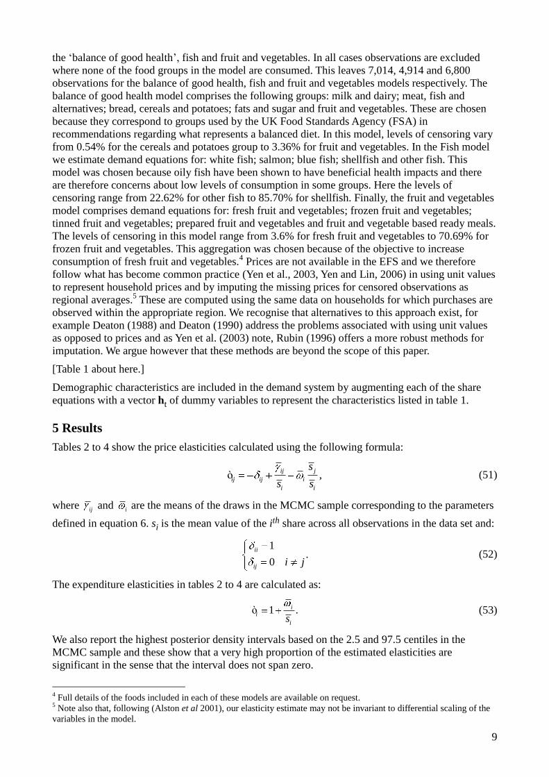
Tables 2 to 4 show the price elasticities calculated using the following formula:

,ij j

ij ij i

i i

s

s sò (51)

where ij and i are the means of the draws in the MCMC sample corresponding to the parameters

defined in equation 6. si is the mean value of the ith share across all observations in the data set and:

0

.1ii

ij i j (52)

The expenditure elasticities in tables 2 to 4 are calculated as:

1 .ii

isò (53)

We also report the highest posterior density intervals based on the 2.5 and 97.5 centiles in the

MCMC sample and these show that a very high proportion of the estimated elasticities are

significant in the sense that the interval does not span zero.

4 Full details of the foods included in each of these models are available on request.

5 Note also that, following (Alston et al 2001), our elasticity estimate may not be invariant to differential scaling of the

variables in the model.

10

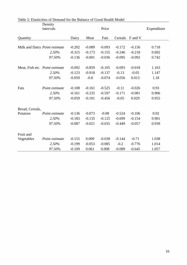
The elasticities for the balance of good health model that are reported in table 2

[Table 2 about here.]

show that all of the foods are own price inelastic with milk and dairy the least responsive and meat

and fish the most responsive. All of the significant cross price effects show the goods to be

complementary emphasising the importance of the income effect in determining cross price

responsiveness. This is a pattern that is repeated in the other two models albeit to a lesser extent and

it raises questions about the use of differential pricing through taxation and subsidies in order to

induce substitution from healthy to unhealthy foods. For example there is a comparatively strong

complementary relationship between the price of fruit and vegetables and the quantity of cereals,

bread and potatoes. Thus a subsidy on fruit and vegetables may be expected to have an undesirable

impact on the quantity consumed of high calorie cereals, bread and potatoes. The effects may not all

be undesirable: there is also a comparatively strong complementarity between the price of fats and

sugars, a group which includes butter, jams, biscuits cakes and sweets, and meats, fish etc. This

suggests that a “fat tax” may also have a beneficial impact in reducing consumption of red meats.

The large number of complementary relationship may be unexpected. We do not report the Hicksian

elasticities in the interests of brevity but examination of these reveals that, without exception, the

compensated cross price effects are all substitutes. Thus we attribute the preponderance of

complementarity to the expenditure effects.

The expenditure elasticities show the impacts on demand for the individual goods of changes in

expenditure on all foods within the system in question. These indicate therefore the relative effects

of changes in income on the different food groups although we would expect the magnitude of the

true income elasticities of demand to be smaller than these expenditure elasticities.6 Milk and dairy,

fats and sugar and cereals bread and potatoes are expenditure inelastic whilst meat, fish etc and fruit

and vegetables are expenditure elastic. This implies that households with higher levels of

expenditure will consume a relatively higher proportion of meat and of fruit and vegetables.

[Table 3 about here.]

In table 3 we see that all fish except for shellfish are own price inelastic. The table also shows that

all fish except shellfish are income inelastic. Blue fish and salmon are unusual in so far as they run

counter to the general pattern of complementarity that is observed in the majority of cases. The fact

that these two are substitutes is perhaps not surprising given that they are both oily fish. The

expenditure elasticities suggest that there is likely to be a higher proportion of oily fish in

comparison with white fish in the diets of high income households.

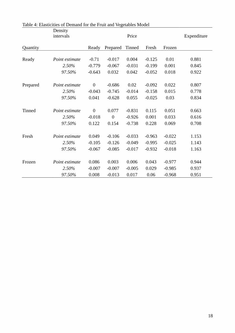
[Table 4 about here.]

Table 4 also shows that all of the groups within this category are price inelastic. The most notable

feature of these results from the dietary health perspective is that the only expenditure elastic group

is fresh fruit and vegetables. Thus not only do higher income households spend proportionately

more on fruit and vegetables as a whole (c.f. table 2) but within the fruit and vegetable category

they spend proportionately more on the fresh products.

[Table 5 about here]

We turn now to the effects of the demographic variables on demand. We report results in table 5 for

the food groups in the balance of good health model. We also indicate with an asterisk when the

95% highest posterior density interval excludes zero as a measure of the significance of the results.

The effects are estimated as the coefficients on dummy variables in the share equations and

converted so that they measure the marginal effect on consumption over a two week period in

natural units at the mean shares and prices across all households. All of the results show the effect

6 The true income elasticity is the product of the expenditure elasticities which we report and the elasticity of food

expenditure with respect to income. We expect the latter to be inelastic and as a result the true income elasticities for the

food groups which we examine are expected to be smaller in magnitude than the results we report.

11

relative to the reference group defined in table 1. The values are based on the mean values of the

parameters in the Gibbs sample. The results show that household composition has an impact across

all of the food groupings. The presence of children in a household leads to a lower level of demand

for fruit and vegetables and meat and increased demand for milk and dairy and cereals and potatoes.

The demographic group has the most significant impacts on cereals and potato and on fruit and

vegetable demand, where there is evidence that lower demographic groups substitute fruit and

vegetables with cereals and potatoes. Demand for fats and sugar and for fruit and vegetables

increases with age whilst demand for cereals and potatoes falls. Regional variation in the demand

for fruit and vegetables is pronounced with the highest demand in London and the South East and

the lowest in Scotland and Northern Ireland. Where the woman is responsible for food purchases,

demand for fats and sugar and for fruit and vegetables is increased whilst that for meat is reduced.

Ethnicity has the most significant impact on demand for fruit and vegetables with increased demand

amongst all groups in comparison with the reference white households.

6 Conclusions

We have demonstrated how the infrequency of purchase model can be estimated for a system of

equations using Monte Carlo Markov chain methods. The method has been illustrated by estimating

a model which is designed to disentangle the impacts of economic factors from preference

heterogeneity resulting from differing demographic conditions in influencing the healthiness of

diets in England and Wales.

Our results imply that households which have a higher level of expenditure will tend to consume

proportionately more meat and more fresh fruit and vegetables. Households in London and the

South East have higher levels of fruit and vegetable consumption whilst it is reduced by the

presence of children. Households employed in the professional or managerial sectors also have

higher levels of fruit and vegetable consumption. Age has an influence on the consumption of fats

and sugars with consumption declining amongst older households. Age also has an impact on the

types of fruit and vegetables consumed with younger households preferring more ready meals and

prepared fruit and vegetables.

Overall the results emphasise the role played by low incomes and socio-economic circumstances in

poor dietary choices. Taking the example of fruit and vegetables we have shown that, comparing an

unemployed individual with an otherwise identical individual living in a household of two, we

would expect the former to consume over 3kg less fruit. Similarly, for two identical households a

difference in income of 10% can be expected to lead to a difference in demand for fruit and

vegetables of around 500g. The other aspect of the results which is especially important in a policy

context is the effect of the presence of children in households. Remaining with the example of fruit

and vegetables, comparing a two person household with children with one without them would

reveal an average level of fruit and vegetable demand which is almost 2kg higher in the childless

family. These patterns are repeated across all of the dietary components that we have analysed and

have important implications for policy makers. There are clear distributional implications for

dietary health that arise from these patterns of consumption and also for the health of children. They

suggest that targeted interventions are necessary in order to reduce the incidence of diet related

health problems in the future.

Acknowledgements

We are grateful to two anonymous referees for helpful suggestions in improving this paper and to

the Food Standards Agency for providing financial support in the early stages of this research.

Andreas Anastassiou worked on early versions of the code used in estimating the models.

References

J.H. Albert and S. Chib. (1993) Bayesian Analysis of Binary and Polychotomous Response Data.

12

Journal of the American Statistical Association 88:669–679.

Alston J.M., J.A. Chalfant, and N.E. Piggott. (2001) Incorporating Demand Shifters in the Almost

Ideal Demand System. Economics Letters 70:73–78.

Amemiya T. (1974) Multivariate Regression and Simultaneous Equation Models when Dependent

Variables are Truncated Normal. Econometrica 42:999 – 1012.

Blundell R. and C. Meghir. (1987) Bivariate Alternatives to the Tobit-model. Journal of

Econometrics 34:179 – 200.

Casella G. and E. I. George. (1992) Explaining the Gibbs Sampler. The American Statistician

46:167–174.

Cragg J.G. (1971) Some Statistical Models for Limited Dependent Variables with Application to

Demand for Durable Goods. Econometrica 39:829 – 844.

Deaton A. (1988) Quality, Quantity and Spatial Variation of Price. American Economic Review

78:418–430.

Deaton A. (1990) Price elasticities from survey data: Extensions and Indonesian results. Journal

of Econometrics 44:281–309.

Dowler E. (2003) Food and poverty. Development Policy Review 21:569–580.

Drewnowski A. (2004) Obesity and the food environment - dietary energy density and diet costs.

American Journal of Preventive Medicine 27:154 – 162.

Geweke J. (2005) Contemporary Bayesian Econometrics and Statistics. New Jersey, US: Wiley.

Heckman J.J. (1979) Sample selection bias as a specification error. Econometrica 47:153–161.

Heien D. and C.R. Wessells. (1990) Demand systems estimation with microdata - a censored

regression approach. Journal of Business and Economic Statistics 8:365 – 371.

Phaneuf D.J. C.L. Kling, and J.A. Herriges. (2000) Estimation and welfare calculations in a

generalized corner solution model with an application to recreation demand. Review of Economics

and Statistics 82:83–92.

Pudney S. (1989) Modelling Individual Choice: The Econometrics of Corners Kinks and Holes.

Oxford, UK: Blackwell.

Rubin D.B. (1996) Multiple imputation after 18+ years. Journal of the American Statistical

Association 91:473–89.

Shonkwiler J.S. and S.T. Yen. (1999) Two-step estimation of a censored system of equations.

American Journal of Agricultural Economics 81:972 – 982.

Stewart H. and S.T. Yen. (2004) Changing household characteristics and the away-from-home

food market: a censored equation system approach. Food Policy 29:643 – 658.

Tanner M.A. and W.H. Wong. (1987) The calculation of the posterior distribution by data

augmentation (with discussion). Journal of the American Statistical Association 82:528–550.

Tobin J. (1958) Estimation of relationships for limited dependent variables. Econometrica 26:24–

36.

Wales T.J. and A.D. Woodland. (1983) Estimation of consumer demand systems with binding

non-negativity constraints. Journal of Econometrics 21:263 – 285.

Yen S.T. (2005) A multivariate sample-selection model: Estimating cigarette and alcohol demands

with zero observations. American Journal of Agricultural Economics 87:453 – 466.

Yen S.T. and B.H. Lin. (2006) A sample selection approach to censored demand systems.

American Journal of Agricultural Economics 88:742 – 749.

13

Yen S.T. B.H. Lin, and D.M. Smallwood. (2003) Quasi- and simulated-likelihood approaches to

censored demand systems: Food consumption by food stamp recipients in the United States.

American Journal of Agricultural Economics 85:458 – 478.

Zellner A. (1971) An Introduction to Bayesian Analysis in Econometrics. New York, US: Wiley

(reprinted 1996 as "Wiley Classics" edition).

14

List of Tables

1 Demographic Variables Included in the Share Equations

2 Elasticities of Demand for the Balance of Good Health Model

3 Elasticities of Demand for the Fish Model

4 Elasticities of Demand for the Fruit and Vegetables Model

5 Effects of Socio-demographic Variables on Food Demand

15

Table 1: Demographic Variables Included in the Share Equations

Household

Composition

Adults only* - Single parents - Family with children - Family with children &

more than 2 adults - Family without children & more than 2 adults

Socio-economic

Groupa

High managerial* - Low managerial - Workers-technical - Never

work/unemployed – Students - Other

Agea

(< 30)* – (30-44) – (45-60) – (≥ 60)

GORb

North East – North West & Merseyside – Yorks & Humber – East Midlands –

West Midlands – Eastern – London* – South East – South West – Wales –

Scotland – Northern Ireland

Ethnic Origina

White* – Mixed race – Asian – Black – Other

Gendera

Male* – Female

a Relating to the household reference person (HRP)

b Government Office Region

* indicates the omitted dummy variable in each category, thereby defining

the reference demographic group for interpreting results

16

Table 2: Elasticities of Demand for the Balance of Good Health Model

Density

intervals Price Expenditure

Quantity Dairy Meat Fats Cereals F and V

Milk and Dairy Point estimate -0.202 -0.089 -0.093 -0.172 -0.156 0.718

2.50% -0.315 -0.173 -0.155 -0.246 -0.218 0.692

97.50% -0.136 -0.001 -0.036 -0.095 -0.092 0.742

Meat, Fish etc. Point estimate -0.092 -0.859 -0.105 -0.093 -0.018 1.163

2.50% -0.123 -0.918 -0.137 -0.13 -0.05 1.147

97.50% -0.059 -0.8 -0.074 -0.056 0.013 1.18

Fats Point estimate -0.108 -0.161 -0.525 -0.11 -0.026 0.93

2.50% -0.161 -0.235 -0.597 -0.171 -0.081 0.906

97.50% -0.059 -0.101 -0.456 -0.05 0.029 0.955

Bread, Cereals,

Potatoes Point estimate -0.136 -0.073 -0.08 -0.524 -0.106 0.92

2.50% -0.183 -0.135 -0.125 -0.699 -0.154 0.901

97.50% -0.087 -0.021 -0.035 -0.449 -0.057 0.939

Fruit and

Vegetables Point estimate -0.155 0.009 -0.038 -0.144 -0.71 1.038

2.50% -0.199 -0.053 -0.085 -0.2 -0.776 1.014

97.50% -0.109 0.061 0.008 -0.089 -0.645 1.057

17

Table 3: Elasticities of Demand for the Fish Model

Density

intervals Price Expenditure

Quantity White Salmon Blue Shell Other

White Point estimate -0.918 0.039 0.011 0.152 0.06 0.873

2.50% -1.029 -0.061 -0.079 0.057 -0.017 0.825

97.50% -0.811 0.155 0.1 0.252 0.128 0.924

Salmon Point estimate 0.016 -0.79 0.147 0.026 -0.194 0.924

2.50% -0.115 -0.915 0.022 -0.101 -0.308 0.828

97.50% 0.146 -0.663 0.284 0.161 -0.084 0.992

Blue Point estimate -0.007 0.174 -0.771 -0.099 -0.06 0.913

2.50% -0.145 0.042 -0.907 -0.259 -0.162 0.818

97.50% 0.132 0.31 -0.635 0.056 0.045 1.013

Shell Point estimate -0.075 -0.168 -0.265 -1.041 -0.324 1.321

2.50% -0.212 -0.302 -0.407 -1.224 -0.434 1.194

97.50% 0.074 -0.027 -0.13 -0.857 -0.2 1.439

Other Point estimate -0.022 -0.163 -0.069 -0.053 -0.673 0.993

2.50% -0.077 -0.218 -0.115 -0.094 -0.739 0.96

97.50% 0.024 -0.111 -0.021 -0.012 -0.59 1.031

18

Table 4: Elasticities of Demand for the Fruit and Vegetables Model

Density

intervals Price Expenditure

Quantity Ready Prepared Tinned Fresh Frozen

Ready Point estimate -0.71 -0.017 0.004 -0.125 0.01 0.881

2.50% -0.779 -0.067 -0.031 -0.199 0.001 0.845

97.50% -0.643 0.032 0.042 -0.052 0.018 0.922

Prepared Point estimate 0 -0.686 0.02 -0.092 0.022 0.807

2.50% -0.043 -0.745 -0.014 -0.158 0.015 0.778

97.50% 0.041 -0.628 0.055 -0.025 0.03 0.834

Tinned Point estimate 0 0.077 -0.831 0.115 0.051 0.663

2.50% -0.018 0 -0.926 0.001 0.033 0.616

97.50% 0.122 0.154 -0.738 0.228 0.069 0.708

Fresh Point estimate 0.049 -0.106 -0.033 -0.963 -0.022 1.153

2.50% -0.105 -0.126 -0.049 -0.995 -0.025 1.143

97.50% -0.067 -0.085 -0.017 -0.932 -0.018 1.163

Frozen Point estimate 0.086 0.003 0.006 0.043 -0.977 0.944

2.50% -0.007 -0.007 -0.005 0.029 -0.985 0.937

97.50% 0.008 -0.013 0.017 0.06 -0.968 0.951

19

Table 5: Effects of Socio-demographic Variables on Food Demand (asterisk indicates that the 95%

highest posterior density interval does not include zero).

Milk and

Dairy (ml) Meat (g)

Fats and

Sugar (g)

Cereals

and Potato

(g)

Fruit and

Veg. (g)

Composition 1 or 2 adults only - - - - -

Single parents 1595.67* -741.56* 614.84* 1732.67* -1989.88*

Children, 2 adults 3011.05* -1054.63* 751.38* 1399.89* -1917.19*

Children, >2 adults 2327.19* -909.17* 328.85 2644.41* -2367.46*

>2 adults, no children 1416.25* -498.80* 141.49 1429.81* -1286.58*

Demographic High managerial - - - - -

group Low managerial -116.14 165.88 92.86 508.62* -1146.25*

Workers-technical -512.24 404.40* 178.57 1437.68* -2759.69*

Never worked-unemp. 441.17 178.02 -6.59 2188.80* -3144.59*

Students -1124.16 303.64 -21.98 1463.92* -1684.44*

Other -522.64 149.51 614.29* 310.21 -1690.08*

Age Under 30 - - - - -

Between 30 and 45 -836.40* 297.28* 382.42* -1695.93* 710.63*

Between 45 and 60 -139.54 279.17* 781.33* -3569.79* 1504.11*

Over 60 365.76 259.52 1161.01* -4642.67* 1606.11*

Region North East -602.38 415.96* 173.90 760.04* -1997.21*

NW & Merseyside 205.42 293.62* 243.68 178.99 -1683.88*

Yorks. & Humber 40.74 113.67 345.33* 219.40 -1302.36*

East Midlands 656.99 -100.38 467.04* -55.64 -1031.85*

West Midlands 186.35 229.65 242.31 -74.53 -1209.94*

Eastern 296.42 44.12 196.71 -266.12 -439.57

London - - - - -

South East 650.05* -125.42 175.28 -586.83* 214.71

South West 702.06 -144.69 565.94* -556.39* -596.80*

Wales -292.96 446.21* 291.49 -165.87 -1534.54*

Scotland -342.36 251.23 393.69* 783.14* -2160.64*

Northern Ireland -200.22 1.93 314.29* 1787.26* -2438.47*

Sex Men - - - - -

Women -3.47 -208.65* 137.91* -224.65 570.87*

Ethnicity White - - - - -

Mixed -1502.06 -410.56 -954.68* 681.83 3403.82*

Asian -154.28 -1218.01* -90.11 735.90 3057.81*

Black -2480.61* 326.18 -292.59 -689.71 1999.46*

Other -3109.86* 387.44 -134.89 -2767.76* 4137.00*