Embed Size (px)
Citation preview
The Dead time correction for the light curve with millisecond time bin
Liang, Jau-shian
Institute of Physics, NTHU
2006/12/5
Reference
• K. Jahoda, J. H. Swank, et al., 1996 Proc. SPIE 2808, p. 59
• K. Jahoda, M. J. Stark, et al., 1999, Nucl. Phys. B (Proc. Suppl.), 69, 210
• Dennis Wei, 2006. Senior Thesis submitted to the MIT Dept. of Physics
• K. Jahoda, C. B. Markwardt, et al., 2006, ApJS, 163, 401

Outline
• Introduction• Recovery method
• Discussion
• Summary

Proportional counter
A proportional counter is a measurement device to count particles and photons of ionizing radiation and measure their energy.

Cross section view of one PCA detector
collimators
propane layer
xenon layer 1xenon layer 2
xenon layer 3
xenon veto layer

The propane layer is principally intended to act as a veto layer to reduce the background rate but could be used as a lower energy detector.
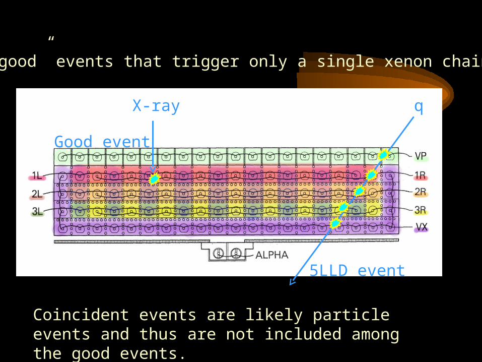
The “good” events that trigger only a single xenon chain.
Coincident events are likely particle events and thus are not included among the good events.
X-ray
Good event
q
5LLD event

• If the source is very bright, there is a non-negligible probability that two photons will arrive within the anti-coincidence window of each other, causing the PCA to mistakenly disqualify both photons.
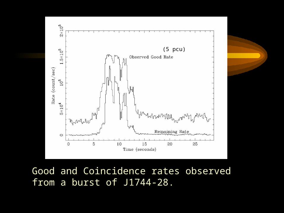
Good and Coincidence rates observedfrom a burst of J1744-28.
(5 pcu)

Remaining rate vs Good rate for a burst from J1744-28
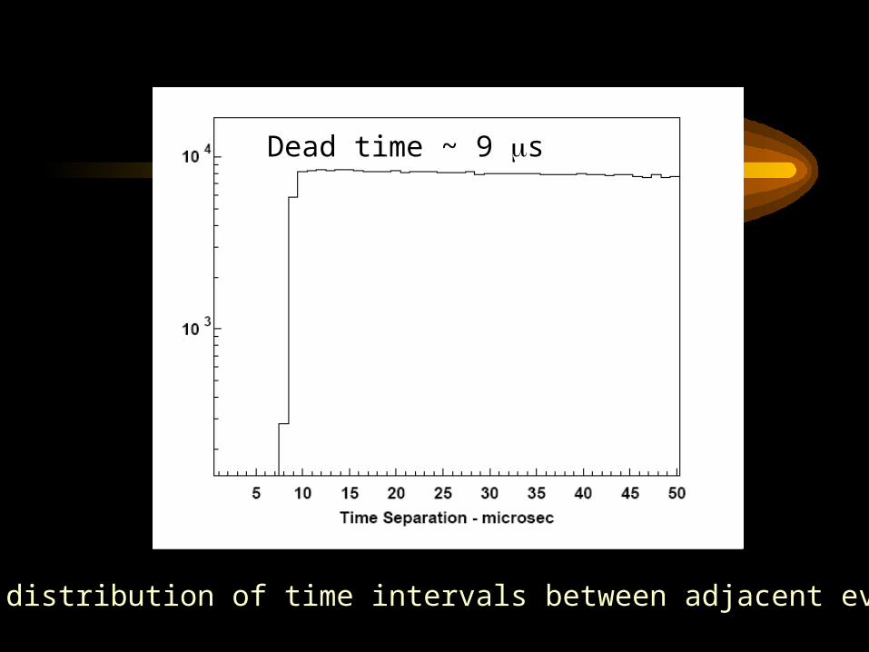
The distribution of time intervals between adjacent events
Dead time ~ 9 s
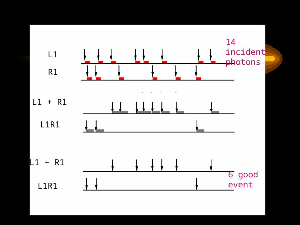
L1 + R1
L1R1
L1
R1
14 incident photons
L1 + R1
L1R16 good event
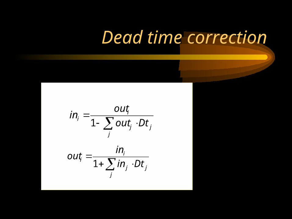
jjj
ii Dtout
outin
1
jjj
ii Dtin
inout
1
Dead time correction
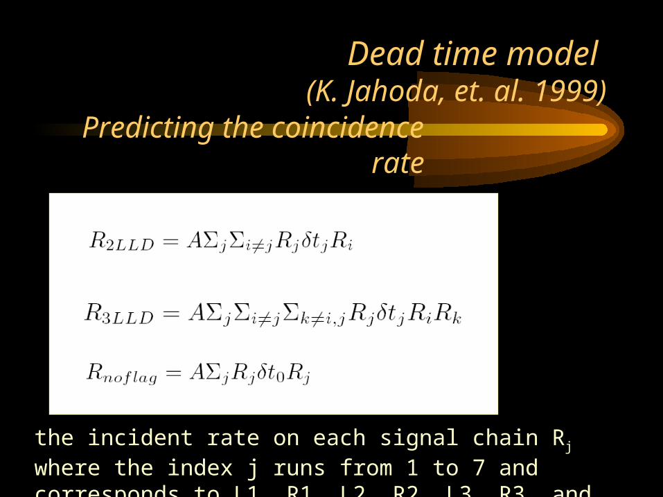
the incident rate on each signal chain Rj where the index j runs from 1 to 7 and corresponds to L1, R1, L2, R2, L3, R3, and VP.
Dead time model (K. Jahoda, et. al. 1999)
Predicting the coincidence rate
1
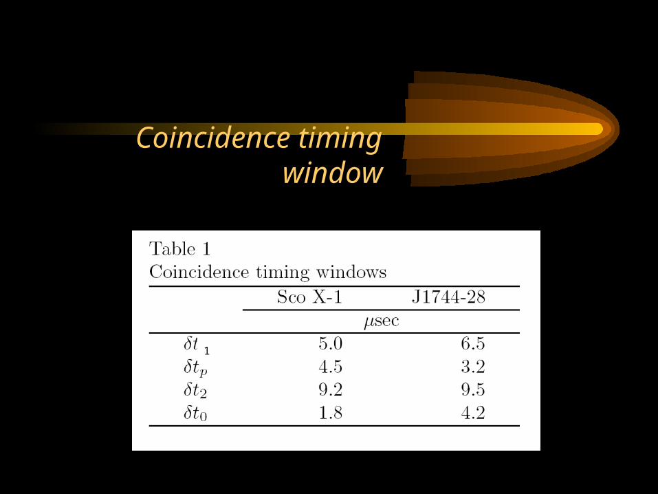
Coincidence timing window

• There is not enough information to do dead time correction with millisecond time resolution.
• The missed coincidence photons should be added in.
• An available way is to construct a recovery method which needs only good rate.
Recovery method

10056-01-01-00 Blank sky #2
(Counts/s/PCU) (Counts/s/PCU)
Good 17800 35
VP 3800 70
Remaining 3400 700 2LLD 1900 80
3-8LLD 750 560
0LLD 360 0-5
VX 440 25
VLE 100 90

assumptions
• The 7 anodes are simplified into 3 anodes (VP, L1 and R1).
• The background of VP, L1 and R1 can be neglected.• The VP rate is proportional to the incident xenon rate.
VP=2Xe
L1=Xe R1=Xe
)(0
0 XeeXe )(220
0
2
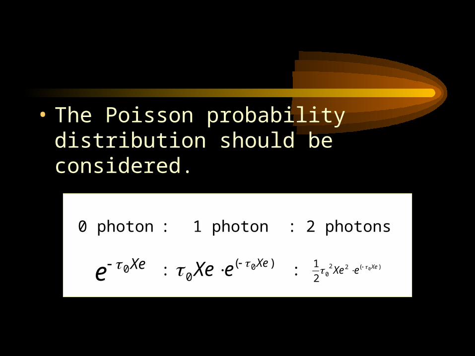
1 XeeXe Xee 0 : :
0 photon : 1 photon : 2 photons
• The Poisson probability distribution should be considered.

L1 R1 VP
L1R1
R1L1
R1VP
L1VP
VPR1
VPL1
0LLD(R1)
0LLD(L1)
0LLD(VP)
)( 0 XeeXe )( 0 XeeXe )( 0 XeeXe )( 0 XeeXe
)( 0 XeeXe )( 0VPeVP )( 0 XeeXe
)( 0 XeeXe )( 0 XeeXe
)( 0VPeVP )( 0VPeVP )( 0VPeVP
Xee 1
VPpe
VPpe
VPpe
VPpe
Xee 1
Xee 1
Xee 1
Xee 1
Xee 1
Xee 1
Xee 1
)(20
0
2
1 XeeXe
)(20
0
2
1 XeeXe
)(20
0
2
1 VPeVP
• The probability of that the photon does not exist should also be considered.

VPXe peeXeRL 0221211
)(1
01)(2 VPXeXep eeVPXeVPXe
XeVPXeVPXe eeVPeeeXeLLD p 1010 220
20 2
10
The prediction of the coincidence rate
•The parameters provided by K. Jahoda et al. are pressumed correct.
5s9s
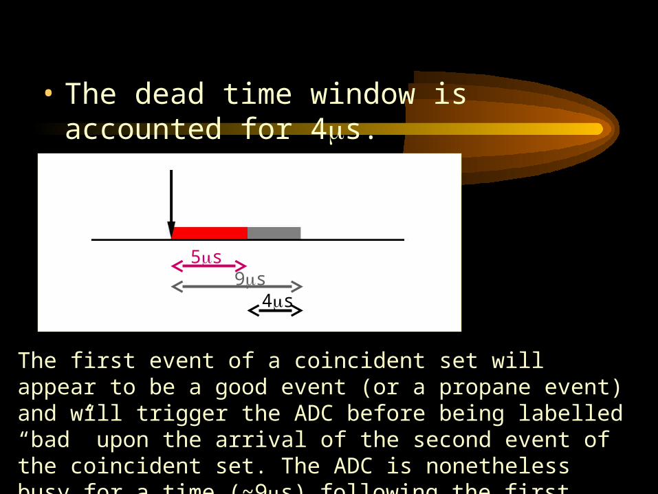
4s
The first event of a coincident set will appear to be a good event (or a propane event) and will trigger the ADC before being labelled “bad” upon the arrival of the second event of the coincident set. The ADC is nonetheless busy for a time (~9s) following the first event of the coincident set. (D. Wei, 2006)
• The dead time window is accounted for 4s.
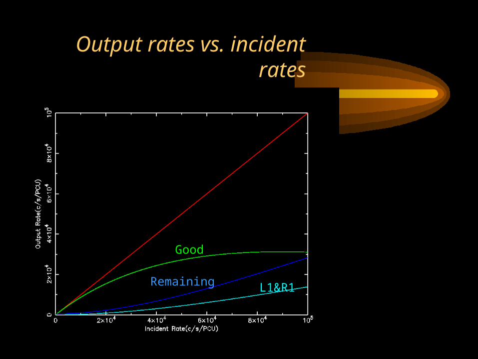
Good
Remaining L1&R1
Output rates vs. incident rates

Estimate and subtractVP, 2LLD, 0LLD
Caculate dead time
X’out = Xout ?
Adjust Xin
Output Xin
Yes
No
Xin

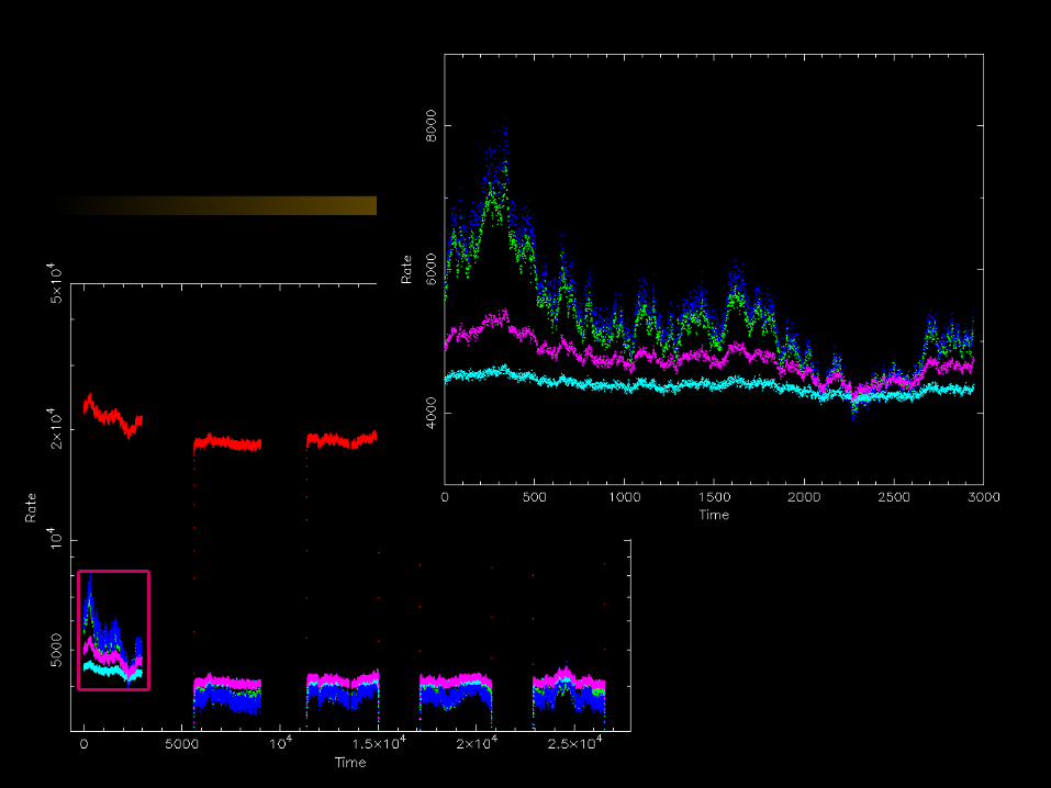
Prediction rates compare with slew data
Good
Remaining(data)Remaining(prediction)
VP(data)VP(prediction)
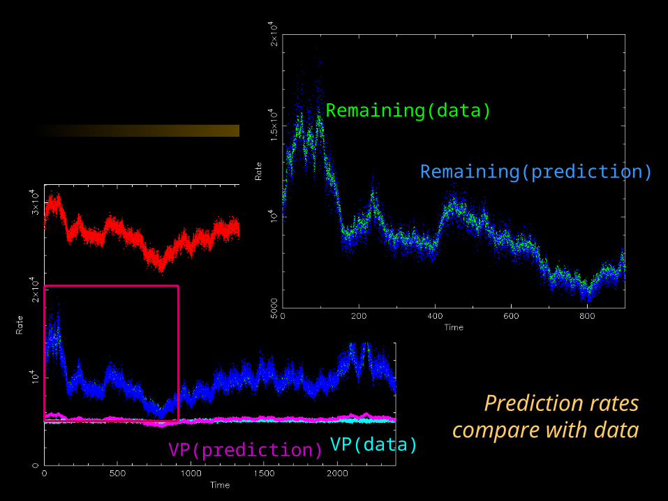
Prediction rates compare with data
Remaining(data)
Remaining(prediction)
VP(data)VP(prediction)

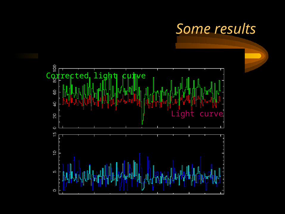
Light curve
Corrected light curve
Some results
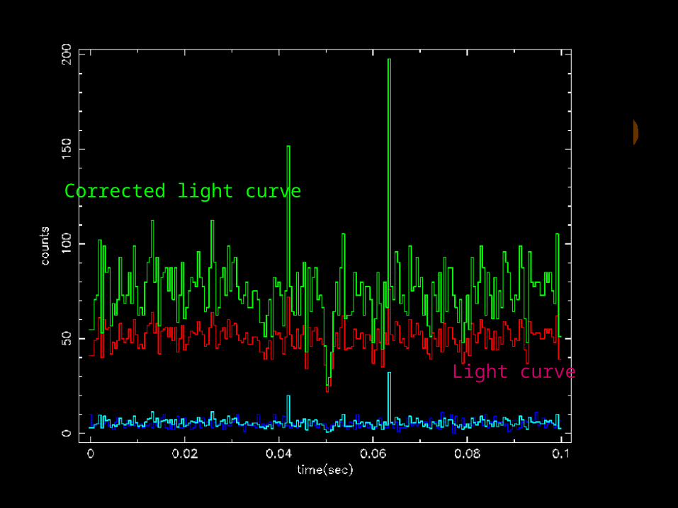
Light curve
Corrected light curve
Discussion
• the advantages and weaknesses
• Are the dips possibly caused by bursts?
• particle bursts within milliseconds?

the advantages and weaknesses
• The prediction rates agree with the data well.
• The light curve can be corrected with only the observed good rate even blow the time scale 1/8s.
the advantages

the weaknesses
• Particle background is still unknown.
• The fluctuation is enlarged.
• Incident propane rate to incident xenon rate ratio is not constant.
• The parameters may be depend on the spectrum.
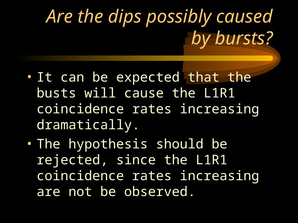
Are the dips possibly caused by bursts?
• It can be expected that the busts will cause the L1R1 coincidence rates increasing dramatically.
• The hypothesis should be rejected, since the L1R1 coincidence rates increasing are not be observed.

particle bursts within milliseconds?
• If the particles come in densely, that will also make the detector blind.
Good counts
particles

T. A. Jones inferred that these energetic events may be the consequence of particle showers produced in the RXTE spacecraft by cosmic rays.

•There are some indications that the events may caused by high energy particles.

Summary
• The light curve can be corrected with only the observed good rate even blow the time scale 1/8s.
• The burst hypothesis has been rejected, since the L1R1 coincidence rates increasing are not be observed.
• The millisecond dips may caused by high energy particles.