Embed Size (px)
Citation preview
The cost of equity for RIIO-2
A review of the evidence
Prepared for Energy Networks Association
28 February 2018
www.oxera.com

Oxera Consulting LLP is a limited liability partnership registered in England no. OC392464, registered office: Park Central, 40/41 Park End Street, Oxford OX1 1JD, UK; in Belgium, no. 0651 990 151, registered office: Avenue Louise 81, 1050 Brussels, Belgium; and in Italy, REA no. RM - 1530473, registered office: Via delle Quattro Fontane 15, 00184 Rome, Italy. Oxera Consulting GmbH is registered in Germany, no. HRB 148781 B (Local Court of Charlottenburg), registered office: Rahel-Hirsch-Straße 10, Berlin 10557, Germany.
Although every effort has been made to ensure the accuracy of the material and the integrity of the analysis presented herein, Oxera accepts no liability for any actions taken on the basis of its contents.
No Oxera entity is either authorised or regulated by the Financial Conduct Authority or the Prudential Regulation Authority within
the UK or any other financial authority applicable in other countries. Anyone considering a specific investment should consult their own broker or other investment adviser. Oxera accepts no liability for any specific investment decision, which must be at the investor’s own risk.
© Oxera 2018. All rights reserved. Except for the quotation of short passages for the purposes of criticism or review, no part may be used or reproduced without permission.
The cost of equity for RIIO-2 Oxera
Contents
Executive summary 1
1 Introduction 9
2 Market parameters: the risk-free rate, total market return, and equity risk premium 11
2.1 Risk-free rate 11 2.2 Total market return and equity risk premium 14 2.3 Conclusion 33
3 Risk and beta 36
3.1 Choice of comparators 36 3.2 Technical estimation issues 38 3.3 Gearing and the relationship between equity beta and asset
beta 40 3.4 Estimation results 40 3.5 Concluding remarks: risk and CAPM-based beta estimates 44
4 Required equity returns for RIIO-2 46
4.1 Reducing the risk of underinvestment 46 4.2 Providing a stable framework for long-term investment 47 4.3 Summary of the CAPM cost of equity estimates 47
5 Alternative sources of evidence 49
5.1 Asset risk premium 49 5.2 Individual stock dividend discount model 49 5.3 Regulatory precedent 50 5.4 Conclusion 54
6 Cost of equity indexation 55
6.1 Indexation of the market parameters 56 6.2 Conclusion 57
A1 Methodologies for estimating the cost of equity 58
A1.1 The capital asset pricing model 58 A1.2 Conclusion 60
The cost of equity for RIIO-2 Oxera
3
Figures and tables
Box 2.1 Geometric versus arithmetic means 19
Box A1.1 The capital asset pricing model 58
Box A1.2 Arbitrage pricing theory 59
Box A1.3 Fama–French three-factor model 60
Figure 2.1 Nominal spot rates on government bonds 11
Figure 2.2 Nominal and real forward rates derived from the nominal yield curve and a 3.0% inflation rate 12
Figure 2.3 UK government bond yields: historical volatility 13
Figure 2.4 UK real TMR, 1900–2016 21
Figure 2.5 Real TMR vs real interest rates: DMS analysis, 1900–2012 21
Figure 2.6 Real TMR versus real interest rates: Oxera analysis, 1900–2012 22
Figure 2.7 TMR (nominal) survey data for the USA: Graham & Harvey study 24
Figure 2.8 ERP survey data from Fernandez et al. for the UK and USA 25
Figure 2.9 3i Infrastructure portfolio-weighted average discount rate 25
Figure 2.10 INPP risk capital-weighted average discount rate 26
Figure 2.11 Nominal TMR and ERP based on a DDM for the FTSE All-share index 28
Figure 2.12 Components of the TMR (nominal) 29
Figure 2.13 VAR 10-year expected UK TMR (nominal) 31
Figure 2.14 Historical averages and UK regulatory precedent on the real total market return 31
Figure 2.15 Historical averages and UK regulatory precedent on the ERP 32
Figure 3.1 Daily asset betas (two years) for listed UK comparator companies and Centrica 41
Figure 3.2 Daily asset betas (2 years) for listed European comparator companies 43
Figure 5.1 UK regulatory precedent for the allowed cost of equity since RIIO-1 (post-tax, real) 51
Figure 5.2 UK regulatory precedent for the WACC allowances since RIIO-1 (vanilla, real) 52
Figure 5.3 European regulatory precedent for the cost of equity (post-tax, real) 53
Figure 5.4 European regulatory precedent for the WACC (vanilla, real) 53
Figure 5.5 Allowed return on equity for US investor-owned electric utilities (nominal) 54
Figure 6.1 Components of a cost of equity indexation mechanism 55
Table 2.1 Historical data on the UK economy and financial markets 17
Table 2.2 Model-based estimates of the historical market return 18
The cost of equity for RIIO-2 Oxera
4
Table 3.1 Liquidity measures for European comparators 38
Table 3.2 Equity and asset beta estimates for UK comparators (debt beta = 0.05) 42
Table 3.3 Equity and asset beta estimates for European comparators (debt beta = 0.05) 44
Table 4.1 Cost of equity for RIIO-2 (real, RPI-deflated) 47
Table 5.1 DDM cost of equity estimates (%) 49
Table 6.1 Options for cost of equity indexation 55
The cost of equity for RIIO-2 Oxera
1
Executive summary
In preparation for the upcoming RIIO-2 electricity and gas transmission and distribution price controls, the Energy Networks Association (ENA) has commissioned Oxera to provide advice on issues relating to the cost of equity.
This report sets out a framework for applying the capital asset pricing model (CAPM) in the context of setting allowed returns for long-lived network investments during RIIO-2. The estimated range for the required equity returns based on the CAPM is compared against alternative sources of evidence on the cost of equity.
There are a number of challenges when determining appropriate estimates of the parameters of the CAPM for RIIO-2. For example:
how to translate from current market data on government bond yields into a risk-free rate (RFR) assumption that will remain valid for the period up to at least 2026 and potentially as far as 2031;1
how to account for the possibility that ‘flight to safety’ effects have increased the equity risk premium (ERP) and thereby mitigated the impact of low RFRs on the expected equity market return;
how to determine an asset beta when the only UK energy network with an equity market listing (National Grid) derives less than half of its revenues from businesses regulated under the RIIO framework.
The way these challenges have been addressed in this report is summarised below. This report also considers some of the implications for the concept of indexing the allowance for the cost of equity, rather than fixing the allowance for the duration of the price control period.
The start of RIIO-2 is more than three years away, therefore the analysis provided in this report is based on current data and may alter by the time the next price controls start.
Risk-free rate
Real, RPI-deflated rates on government bonds of ten-year maturity are currently negative, at around -1.5%. Throughout the expected period of the RIIO-2 price controls (2021–31), the implied forward rate is around -0.5% on average. While interest rates are low, they exhibit marked volatility, such that setting the allowed RFR for RIIO-2 exactly equal to the level of forward rates may not be appropriate. This consideration is especially relevant in the context of current unusual monetary policy and uncertainty in relation to the pace and timing of future changes in the quantitative easing programme and its resulting effect on interest rates.
As the start of RIIO-2 is over three years away, an initial estimate for the RFR (real, RPI-deflated) of -0.5 to 0.0% appears appropriate based on forward rates and allowing for volatility and uncertainty. We suggest that the evidence is monitored to ensure that it is incorporated into the final estimate of the cost of equity for RIIO-2, although it will still be necessary to allow for uncertainty regarding market developments during the RIIO-2 price control period.
1 RIIO-T2/GD2 starts in 2021 and RIIO-ED2 starts in 2023. These controls would finish in 2029 and 2031 respectively if the length of the control period remains eight years.

The cost of equity for RIIO-2 Oxera
2
The estimation of the RFR cannot be considered in isolation from the ERP. A central conclusion of this report is that the RFR and ERP are negatively correlated, with the result that the total market return (TMR) is more stable than the ERP alone.
Equity risk premium and total market return
Forming a precise view on the real expected TMR is made challenging by the wide range of estimates from the various sources of evidence. The central issue in the current debate over the TMR is the degree to which the expected ERP adjusts to offset changes in the RFR. The theoretical and empirical evidence basis for assuming a stable ERP appears weak.
Consumption-based asset pricing models find that higher economic uncertainty simultaneously places downward pressure on the RFR and upward pressure on the ERP.2
Historical data shows that the RFR and ERP have been very volatile while total equity market returns have been relatively more stable over time, and calls into question the assertion that equity markets are going through a period of ‘secular stagnation’.3
Estimates from dividend discount models (DDMs) suggest that the TMR is relatively stable over time and is currently no lower than its estimated value in the early 2000s.
The reliability of survey evidence and discount rate assumptions used by infrastructure funds is lower than more direct market evidence, but is inconclusive about whether the ERP or the TMR is the more stable parameter.
This suggests that an appropriate TMR assumption would place more weight on the view that the expected TMR is relatively stable, and close to its long-run average of 7.3%,4 than the view that the ERP is close to its long-run average of 4.9% (implying a TMR of 4.4% when combined with forward interest rates, which are on average -0.5% for the RIIO-2 period).5
Attenuation of the upper end of the range—the version of the DDM used by the Bank of England (BoE) indicates a real TMR of at least 7.5%, while the historical arithmetic average of the real TMR from Dimson, Marsh and Staunton (DMS) is 7.3%.6 It might be argued that some weight should be given to the view that the increase in the ERP has not fully offset the decline in the RFR, and as a result, for the purpose of establishing a range for RIIO-2, an attenuated TMR of up to 6.5% is assumed. This is approximately 80bp lower than would be justified by the historical average of the real TMR and 100bp lower than justified by the version of the DDM used by the BoE. The top end of the range is therefore lower than implied by the view that the TMR is completely stable.
Attenuation of the lower end of the range—the historical average of the ERP from DMS (4.9%) combined with forward rates, which are on average -0.5% for the RIIO-2 period, suggests a TMR of 4.4%. It appears likely that
2 Martin, I. (2013), ‘Consumption-Based Asset Pricing with Higher Cumulants’, Review of Economic Studies, 80, pp. 746; Vlieghe, G. (2017), ‘Real interest rates and risk’, Society of Business Economists' Annual conference, 15 September. 3 Òscar, J., Knoll, K., Kuvshinov, D., Schularick, M. and Taylor, A. (2017), ‘The Rate of Return on Everything, 1870–2015’, Federal Reserve Bank of San Francisco Working Paper 2017-25, p. 41. 4 Dimson, E., Marsh, P. and Staunton, M. (2017), 'Credit Suisse Global Investment Returns Yearbook 2017', p. 14. 5 Ibid., p. 31. 6 Ibid., p. 14.
The cost of equity for RIIO-2 Oxera
3
the decrease in the RFR has been associated with an increase in the ERP, and as a result, for the purpose of RIIO-2, an attenuated lower bound of the TMR of 5.5% appears more appropriate. This would position the TMR assumption approximately 110bp higher than would be justified by the historical average of the real ERP combined with forward rates. The lower end of the range is therefore higher than implied by the view that the ERP is completely stable.
This provides an attenuated range of 5.5–6.5% for the real (RPI-deflated) TMR. In combination with an RFR assumption of -0.5–0.0%, this would imply an ERP of 6.0–6.5%. This attenuation of the range has been broadly symmetric and does not take adequate account of the weight of evidence in support of a relatively stable TMR. If the range had not been attenuated, it would have been 4.4–7.4%7 with a midpoint of 5.9%, compared to a 6.0% midpoint of the attenuated range. In light of the fact that both the financial theory and the empirical evidence support a relatively stable TMR with an estimate towards the top end of the range (6.5%), we recommend a range of 6.0–6.5% for the TMR (real, RPI-deflated). Combined with the preliminary recommended range of -0.5–0.0% for the RFR (real, RPI-deflated), this implies an ERP of 6.5%, taking the midpoints of these two parameters.
Selecting a TMR towards the top end of the range is consistent with the view of the Competition Commission in the Northern Ireland Electricity (2014) price control appeal, where a point estimate at the top end of the range for the weighted average cost of capital (WACC) was selected.8 One of the reasons for this choice of point estimate was that the CC was less confident in the numbers at the low end of the TMR range.9
13.187 We consider that the lower bound of 5 per cent for the expected return on the market was less well supported than the upper end of the range of 6.5 per cent. We consider that the weight of evidence tended to support numbers between 5.5 and 6.5 per cent for the expected market return. While we decided to retain 5 per cent as a possibility, we were less confident with this estimate and, as a corollary, with numbers at the low end of the WACC range.
This view was reaffirmed in the Bristol Water (2015) appeal.10
In summary, the updated evidence presented in this report suggests that a range of 6.0–6.5% for the TMR (real, RPI-deflated) is appropriate for RIIO-2.
Risk and beta
The sample of National Grid and three listed water companies produces a range of estimates for the asset beta (un-levered equity beta) of 0.35–0.41 based on the longer-term five-year averages. This assumes a debt beta of 0.05. The shorter-term two-year averages suggest a lower range, of 0.30–0.39, which highlights the sensitivity of the estimates to the choice of measurement period.
These ranges may underestimate the beta for energy networks. The asset beta for National Grid, an energy utility, tends to be higher than that of the two pure-
7 The lower bound (4.4%) is the long-run arithmetic average ERP from Dimson et al. (2017) plus an average forward interest rate of -0.5% for the RIIO-2 period. The upper bound (7.4%) is the average of the long-run arithmetic average TMR (7.3%) from Dimson et al. (2017) and the TMR from the BoE’s DDM (7.5%). 8 Competition Commission (2014), ‘Northern Ireland Electricity Limited; A reference under Article 15 of the Electricity (Northern Ireland) Order 1992’, 26 March, para. 13.187. 9 Competition Commission (2014), op. cit., paras 13.87 and 13.189. 10 Competition and Markets Authority (2015), ‘Bristol Water plc; A reference under Section 12 of the Water Industry Act 1991’, 6 October, para. 10.185.
The cost of equity for RIIO-2 Oxera
4
play water comparators (United Utilities and Severn Trent), and is currently estimated as 0.41 (five-year average) and 0.35 (two-year average).
Decisions taken by UK economic regulators are consistent with the assessment that energy networks face higher systematic risk exposure than water networks. For example, in the RIIO-1 decisions, the asset betas implied by Ofgem’s assumptions for equity betas and gearing were in the range of 0.32–0.43,11 while Ofwat’s contemporaneous PR14 decision regarding the asset beta was 0.30.
There may be an increase in fundamental risk differences between water and energy networks over the RIIO-2 period. Energy networks over RIIO-2 will be accommodating a period of potentially rapid technological change, which will create uncertainty around patterns of expenditure for network reconfiguration. It is unlikely that exposure to such risks can be fully mitigated through regulatory mechanisms (e.g. indexation, pass-through, volume drivers, re-openers, etc.). The residual risk will be borne by equity.
Therefore, as there are limited data points for energy network betas in the UK, and UK water networks may not be representative of the systematic risk exposure of energy networks over the RIIO-2 period, asset beta estimates have also been derived based on a European sample, where the business risk may be closer aligned to that of UK energy networks, notwithstanding the differences in risk across jurisdictions—e.g. due to differences in regulatory regimes. Asset betas for a sample of four European energy networks (Enagas, Red Eléctrica, Snam, Terna) have been assessed, and are in the range of 0.40–0.45 based on the longer-term five-year averages. As with the UK sample, this assumes a debt beta of 0.05. The shorter-term two-year averages suggest a lower range of 0.33–0.42. This points towards a higher asset beta for energy networks compared with the water companies that dominate the UK sample.
On balance, the evidence from the UK and European samples and the five- and two-year averages suggests an attenuated asset beta range of 0.38–0.42. This is consistent with energy networks having greater exposure to risk than water companies.
Tests of the empirical performance of the CAPM have revealed many ‘anomalies’ that suggest that the accuracy of the standard CAPM in predicting the cost of equity decreases the further away the equity beta is from unity.12 In particular, the CAPM tends to under-predict returns for companies with equity betas lower than one. As the comparator companies used in this report have equity betas significantly lower than one when measured at market levels of gearing, adopting an asset beta estimate in the top half of the range would provide some offset to this downward bias.
Furthermore, the literature on arbitrage pricing theory and multi-factor models suggests that there could be systematic risk factors that are not picked up in the CAPM market beta but are nevertheless priced by investors.13 The impact of the wider risk environment faced by energy networks can be accounted for
11 0.43 was the upper end of the range for SHETL/SPTL in RIIO-T1, while the asset beta for NGGT and NGET was lower, at around 0.34–0.38. 12 Asness, C., Moskowitz, T.J. and Pedersen, L.H. (2013), ‘Value and momentum everywhere’, The Journal of Finance, LXVIII:3; Fama, E. and French, K. (2015), ‘Dissecting Anomalies with a Five-Factor Model’, The Review of Financial Studies, 29:1, 1 January 2016, pp. 69–103. 13 Chen, N., Roll, R. and Ross, S. (1986), ‘Economic Forces and the Stock Market’, The Journal of Business, 59:3, pp. 383–403; Ross, S. (1976), ‘The Arbitrage Theory of Capital Asset Pricing’, Journal of Economic Theory, 13, pp. 341–360.

The cost of equity for RIIO-2 Oxera
5
when interpreting the outputs from the CAPM. In the context of UK energy networks, the extent and nature of the changes required to both electricity and gas distribution, and transmission, networks to facilitate energy decarbonisation and the necessary innovations in technologies required have created uncertainty over the future configuration of the energy system.
Consideration of the risks facing energy networks and the empirical shortcomings of the CAPM suggests selecting a beta point estimate in the top half of the attenuated range based on listed comparator companies. We recommend a range of 0.40–0.42 to inform the asset beta assumption for RIIO-2.
The asset beta range has been derived from comparator companies with gearing broadly in the range of 40–50% based on market values. The RIIO-1 price control decisions assumed gearing of 55–65% relative to the regulatory asset value (RAV), which was applied in the calculation of the WACC.14 Therefore, the cost of equity has been calculated in this report using a midpoint gearing assumption of 60% to re-lever the asset beta range. This is to achieve consistency with the second proposition of Modigliani and Miller (1958):
the expected yield of a share of stock is equal to the appropriate [expected rate of return] for a pure equity stream in the class, plus a premium related to financial risk equal to the debt-lo-equity ratio times the spread between [the expected rate of return] and [the risk-free rate of interest].15
With a gearing assumption of 60% and a debt beta assumption of 0.05, an equity beta range of 0.93–0.98 is recommended for RIIO-2.
The higher the notional gearing relative to the gearing ratios for the comparator companies used to derive the asset beta range, the more sensitive the estimation of the re-levered equity beta is to the assumed relationship between debt beta and gearing. Due to this additional estimation uncertainty we therefore do not include a 65% gearing ratio within our recommended range in this report. Were a 65% gearing ratio to be used in RIIO-2 we would expect the equity betas to be higher than the range set out above, but not as high as a simple application of a re-levering formula would imply and would be expected to be close to 1.
Required equity returns for RIIO-2
A range of 5.51–6.34% is recommended to inform the assumption for the real (RPI-deflated) cost of equity in RIIO-2. This takes account of the following factors when moving from the attenuated range to a recommended range.
the attenuated range does not take full account of the weight of evidence in support of a relatively stable TMR;
the attenuated range relies on equity betas estimated for comparator companies that are significantly less than unity. Empirical tests find that the CAPM tends to under-predict returns for companies with equity betas lower than one;
14 Specifically, Ofgem varied the notional gearing ratio assumptions across the UK energy networks—55% for RIIO-T1 (SHETL and SPTL); 60% for RIIO-T1 (NGET); 62.5% for RIIO-T1 (NGGT) and 65% for RIIO-GD1 and RIIO-ED1. 15 Modigliani, F. and Miller, M. (1958), ‘The Cost of Capital, Corporation Finance and the Theory of Investment’, The American Economic Review, 48:3, June, p. 271.
The cost of equity for RIIO-2 Oxera
6
the attenuated range may not fully reflect the wider risk environment faced by energy networks—in particular, the relatively high exposure of the sector to technological and political risks.
When selecting a point estimate within the recommended range, it is important to balance the long-term cost of potentially creating an underinvestment problem against the short-term cost of setting customer prices that are unnecessarily high.
Furthermore, regulated networks make investment decisions and receive returns over very long horizons spanning multiple price control periods, which would be supported by a regulatory regime that has a stable methodology and limits volatility in allowed returns from one price control period to the next. Limiting the change in the allowed return on equity for the RIIO-2 controls compared with the RIIO-1 controls would support long-term investment decisions.
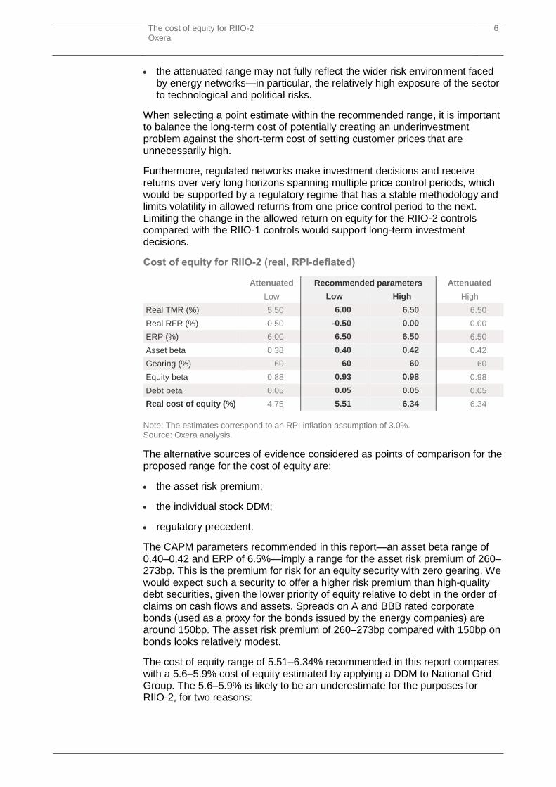
Cost of equity for RIIO-2 (real, RPI-deflated)
Attenuated Recommended parameters Attenuated
Low Low High High
Real TMR (%) 5.50 6.00 6.50 6.50
Real RFR (%) -0.50 -0.50 0.00 0.00
ERP (%) 6.00 6.50 6.50 6.50
Asset beta 0.38 0.40 0.42 0.42
Gearing (%) 60 60 60 60
Equity beta 0.88 0.93 0.98 0.98
Debt beta 0.05 0.05 0.05 0.05
Real cost of equity (%) 4.75 5.51 6.34 6.34
Note: The estimates correspond to an RPI inflation assumption of 3.0%. Source: Oxera analysis.
The alternative sources of evidence considered as points of comparison for the proposed range for the cost of equity are:
the asset risk premium;
the individual stock DDM;
regulatory precedent.
The CAPM parameters recommended in this report—an asset beta range of 0.40–0.42 and ERP of 6.5%—imply a range for the asset risk premium of 260–273bp. This is the premium for risk for an equity security with zero gearing. We would expect such a security to offer a higher risk premium than high-quality debt securities, given the lower priority of equity relative to debt in the order of claims on cash flows and assets. Spreads on A and BBB rated corporate bonds (used as a proxy for the bonds issued by the energy companies) are around 150bp. The asset risk premium of 260–273bp compared with 150bp on bonds looks relatively modest.
The cost of equity range of 5.51–6.34% recommended in this report compares with a 5.6–5.9% cost of equity estimated by applying a DDM to National Grid Group. The 5.6–5.9% is likely to be an underestimate for the purposes for RIIO-2, for two reasons:
The cost of equity for RIIO-2 Oxera
7
the DDM analysis is based on market gearing (net debt/enterprise value) in the range of 40–50%. To inform a RIIO-2 assumption, the cost of equity estimates would need to be re-levered using the regulatory gearing assumption, which, based on the RIIO-1 controls, is likely to be closer to 60%;
the long-term forecasts for UK GDP growth that have been used as an input to the company-specific DDM may be lower than company-specific dividend growth. For example, the real rate of growth observed for the RAV of National Grid Electricity Transmission during RIIO-T1 (around 4% per annum) has exceeded UK GDP growth.
The recent cost of equity determinations by Ofcom and the Northern Ireland Utility Regulator are based on lower gearing assumptions than used in this report, and would be higher and consistent with the range recommended in this report if re-stated based on the 60% gearing assumption used in this report.
The cost of equity range presented by Ofwat in the Final Methodology for PR19 is 3.41–4.69%.16 This is guidance and not a final determination. There are two main differences between the underlying assumptions. The first is the lower asset beta assumed by Ofwat (0.37) for water companies compared with 0.40–0.42 estimated in this report for energy networks.17 As explained in this report, the evidence from betas of comparator energy networks, and the exposure of energy networks to uncertainty relating to energy decarbonisation and the necessary innovations in technologies required, support the use of a higher asset beta relative to water companies. The second is that Ofwat assumes a lower range for the TMR of 4.85–6.13% compared with the range of 6.0–6.5% assumed in this report. The lower TMR assumed by Ofwat is predicated on the assumption that rates of return will remain ‘lower for longer’ and that this translates into a lower expected return on the equity market. As explained in this report, the balance of evidence supports a relatively stable TMR.
Recent European regulatory precedents on the cost of equity span a range from 4.0% to 6.0% (post-tax, real). The range presented in this report corresponds to the top half of European regulatory precedents. The bottom half of European precedents are set by regulators (e.g. in Germany and the Netherlands) that have consistently followed more mechanistic approaches to setting the allowed cost of equity. The Netherlands and Germany respectively use three- and ten-year averages for the RFR and assume a fixed ERP. As market RFRs have declined, this has fed directly into reduced allowances for the cost of equity. As discussed in section 2.2, the theoretical and empirical evidence basis for assuming a stable ERP appears weak.
The most recent allowed returns on equity in the USA are clustered around 9.5% (post-tax, nominal). This is similar to the nominal return on equity allowed by Ofgem in the RIIO-1 price controls. With an RPI inflation assumption of 3%, this translates into a 6.5% cost of equity, which is above the top end of the range presented in this report.
Overall, the alternative sources of evidence support the cost of equity range of 5.51–6.34% (real, RPI-deflated) recommended in this report.
16 Ofwat (2017), ‘Delivering Water 2020: Our final methodology for the 2019 price review’, 13 December, Appendix 12, Table 1. 17 Ofwat presents two asset betas, assuming debt beta of zero and 0.1 respectively. The asset beta assuming debt beta of 0.1 has been presented.
The cost of equity for RIIO-2 Oxera
8
Cost of equity indexation
It has been suggested that the allowed cost of equity be indexed instead of setting an allowance that is fixed for the duration of the price control period. Cost of equity indexation could be used to align the cost of equity allowed by the regulator to the estimated cost of equity in each year of the price control.
The cost of equity is not observable. Therefore, in any attempt to index the cost of equity, a decision needs to be taken about whether (and how) to index one, or several, of the cost of equity parameters. The design of any cost of equity indexation mechanism will involve a higher degree of subjectivity than the equivalent mechanism for the cost of debt.
The following principles for indexing the cost of equity emerge from the evidence examined in this report.
there is a negative correlation between the ERP and the RFR, which implies that indexation of only the RFR would create large errors;
the TMR is relatively stable over time, which implies that the TMR generated by the indexation mechanism should be relatively stable over time;
equity beta estimates are more volatile over time than would be expected given the relatively stable risk characteristics of the businesses. This implies that the beta parameters of the indexation mechanism should be more stable than the market estimates, or should be fixed.
Overall, a move to cost of equity indexation would represent a considerable change in methodology. Such a change in methodology would need to fully take into account the principles above, be appropriately signalled and introduced with appropriate transitional arrangements such that it does not undermine investor confidence.
The cost of equity for RIIO-2 Oxera
9
1 Introduction
In preparation for the upcoming RIIO-2 electricity and gas transmission and distribution price controls, the Energy Networks Association (ENA) has commissioned Oxera to provide advice on issues relating to the cost of equity. RIIO-2 will govern the allowed revenue arrangements for the ENA member organisations.
There are many ways to estimate the cost of equity. By far the most common one used by regulators and practitioners is the capital asset pricing model (CAPM).18 This report estimates the required equity returns for long-lived network asset investments based on the CAPM and considers alternative sources of evidence.
The report analyses a number of the challenges when determining appropriate estimates of the parameters of the CAPM for RIIO-2. For example:
how to translate from current market data on government bond yields into a risk-free rate (RFR) assumption that will remain valid for the period up to at least 2026 and potentially as far as 2031;19
how to account for the possibility that ‘flight to safety’ effects have increased the equity risk premium (ERP) and thereby mitigated the impact of low RFRs on the expected equity market return;
how to determine an asset beta when the only UK energy network with an equity market listing (National Grid) derives less than half of its revenues from businesses regulated under the RIIO framework?
The report is structured as follows.
Section 2 discusses the estimation of the market parameters, considering the current theoretical and empirical evidence on the RFR, total market return (TMR) and ERP. The RFR cannot be considered in isolation from the ERP and TMR.
Section 3 considers the latest evidence on equity betas and gearing, to derive an estimate of the asset beta for energy networks in the UK. It also considers energy sector risks that may not be captured in an equity beta estimate.
Section 4 brings together the evidence from the previous two sections to give an initial cost of equity range for RIIO-2.
Section 5 provides alternative sources of evidence on the estimated required equity returns based on asset risk premia, company-specific dividend discount model (DDM) estimates, UK and international regulatory precedent.
Section 6 discusses cost of equity indexation mechanisms as a potential alternative to setting a fixed allowance.
Appendix A1 evaluates the CAPM and its multi-factor alternatives such as arbitrage pricing theory and other factor models.
18 A more detailed review of the CAPM and its alternatives is provided in Appendix A1. 19 RIIO-T2/GD2 starts in 2021 and would finish in 2026 if the length of the control is shortened to five years. RIIO-ED2 starts in 2023 and would finish in 2031 if the length of the control remains eight years.

The cost of equity for RIIO-2 Oxera
10
The start of RIIO-2 is more than three years away; therefore, the analysis provided in this report is based on current data and may alter by the time the next price controls start.
The cost of equity for RIIO-2 Oxera
11
2 Market parameters: the risk-free rate, total market return, and equity risk premium
This section reviews the estimation of the market parameters (the RFR and the ERP) and their interdependency with the TMR. The TMR is the sum of the RFR and a risk premium for investing in equity; when implementing the CAPM, the estimation of the RFR cannot be considered in isolation from the ERP and TMR.
This section looks at:
the RFR (section 2.1);
the ERP and the evidence for setting the market parameters using either the ERP or the TMR as the anchor for the parameters (section 2.2).
It then concludes on the market parameters (section 2.3).
2.1 Risk-free rate
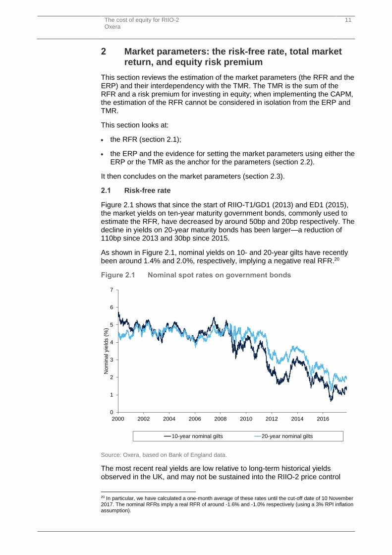
Figure 2.1 shows that since the start of RIIO-T1/GD1 (2013) and ED1 (2015), the market yields on ten-year maturity government bonds, commonly used to estimate the RFR, have decreased by around 50bp and 20bp respectively. The decline in yields on 20-year maturity bonds has been larger—a reduction of 110bp since 2013 and 30bp since 2015.
As shown in Figure 2.1, nominal yields on 10- and 20-year gilts have recently been around 1.4% and 2.0%, respectively, implying a negative real RFR.20
Figure 2.1 Nominal spot rates on government bonds
Source: Oxera, based on Bank of England data.
The most recent real yields are low relative to long-term historical yields observed in the UK, and may not be sustained into the RIIO-2 price control
20 In particular, we have calculated a one-month average of these rates until the cut-off date of 10 November 2017. The nominal RFRs imply a real RFR of around -1.6% and -1.0% respectively (using a 3% RPI inflation assumption).
0
1
2
3
4
5
6
7
2000 2002 2004 2006 2008 2010 2012 2014 2016
No
min
al yie
lds (
%)
10-year nominal gilts 20-year nominal gilts
The cost of equity for RIIO-2 Oxera
12
periods. It is important to consider how to allow for this eventuality in the selection of an appropriate RFR assumption for energy networks in RIIO-2.
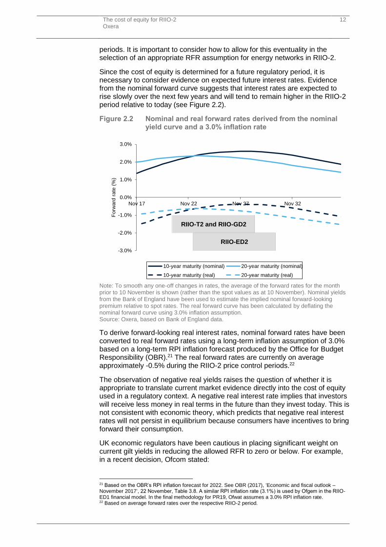
Since the cost of equity is determined for a future regulatory period, it is necessary to consider evidence on expected future interest rates. Evidence from the nominal forward curve suggests that interest rates are expected to rise slowly over the next few years and will tend to remain higher in the RIIO-2 period relative to today (see Figure 2.2).
Figure 2.2 Nominal and real forward rates derived from the nominal yield curve and a 3.0% inflation rate
Note: To smooth any one-off changes in rates, the average of the forward rates for the month prior to 10 November is shown (rather than the spot values as at 10 November). Nominal yields from the Bank of England have been used to estimate the implied nominal forward-looking premium relative to spot rates. The real forward curve has been calculated by deflating the nominal forward curve using 3.0% inflation assumption. Source: Oxera, based on Bank of England data.
To derive forward-looking real interest rates, nominal forward rates have been converted to real forward rates using a long-term inflation assumption of 3.0% based on a long-term RPI inflation forecast produced by the Office for Budget Responsibility (OBR).21 The real forward rates are currently on average approximately -0.5% during the RIIO-2 price control periods.22
The observation of negative real yields raises the question of whether it is appropriate to translate current market evidence directly into the cost of equity used in a regulatory context. A negative real interest rate implies that investors will receive less money in real terms in the future than they invest today. This is not consistent with economic theory, which predicts that negative real interest rates will not persist in equilibrium because consumers have incentives to bring forward their consumption.
UK economic regulators have been cautious in placing significant weight on current gilt yields in reducing the allowed RFR to zero or below. For example, in a recent decision, Ofcom stated:
21 Based on the OBR’s RPI inflation forecast for 2022. See OBR (2017), ‘Economic and fiscal outlook – November 2017‘, 22 November, Table 3.8. A similar RPI inflation rate (3.1%) is used by Ofgem in the RIIO-ED1 financial model. In the final methodology for PR19, Ofwat assumes a 3.0% RPI inflation rate. 22 Based on average forward rates over the respective RIIO-2 period.
-3.0%
-2.0%
-1.0%
0.0%
1.0%
2.0%
3.0%
Nov 17 Nov 22 Nov 27 Nov 32
Fo
rwa
rd r
ate
(%
)
10-year maturity (nominal) 20-year maturity (nominal)
10-year maturity (real) 20-year maturity (real)
RIIO-T2 and RIIO-GD2
RIIO-ED2
The cost of equity for RIIO-2 Oxera
13
We continue to believe that caution is required in interpreting the evidence available. Given that we are attempting to estimate a forward-looking real RFR appropriate for the end of the charge control period, it would be inappropriate to simply adopt the current low rates on index-linked gilts without considering the reasons why they could be depressed.23
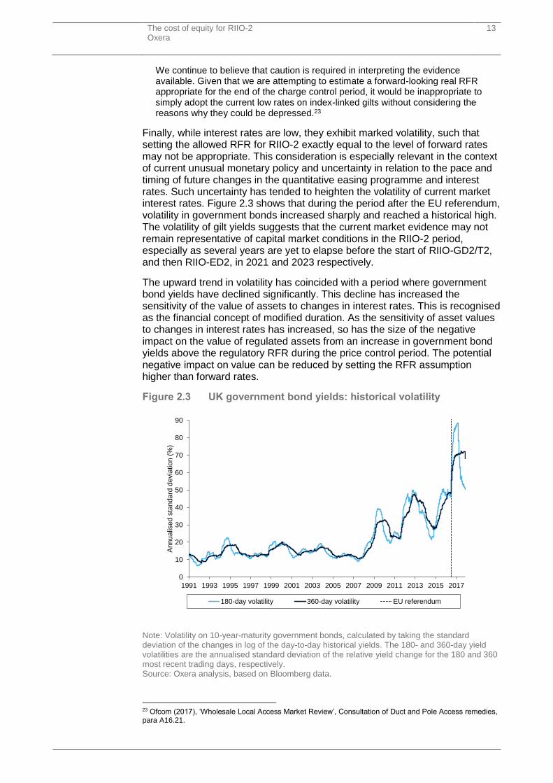
Finally, while interest rates are low, they exhibit marked volatility, such that setting the allowed RFR for RIIO-2 exactly equal to the level of forward rates may not be appropriate. This consideration is especially relevant in the context of current unusual monetary policy and uncertainty in relation to the pace and timing of future changes in the quantitative easing programme and interest rates. Such uncertainty has tended to heighten the volatility of current market interest rates. Figure 2.3 shows that during the period after the EU referendum, volatility in government bonds increased sharply and reached a historical high. The volatility of gilt yields suggests that the current market evidence may not remain representative of capital market conditions in the RIIO-2 period, especially as several years are yet to elapse before the start of RIIO-GD2/T2, and then RIIO-ED2, in 2021 and 2023 respectively.
The upward trend in volatility has coincided with a period where government bond yields have declined significantly. This decline has increased the sensitivity of the value of assets to changes in interest rates. This is recognised as the financial concept of modified duration. As the sensitivity of asset values to changes in interest rates has increased, so has the size of the negative impact on the value of regulated assets from an increase in government bond yields above the regulatory RFR during the price control period. The potential negative impact on value can be reduced by setting the RFR assumption higher than forward rates.
Figure 2.3 UK government bond yields: historical volatility
Note: Volatility on 10-year-maturity government bonds, calculated by taking the standard deviation of the changes in log of the day-to-day historical yields. The 180- and 360-day yield volatilities are the annualised standard deviation of the relative yield change for the 180 and 360 most recent trading days, respectively. Source: Oxera analysis, based on Bloomberg data.
23 Ofcom (2017), ‘Wholesale Local Access Market Review’, Consultation of Duct and Pole Access remedies, para A16.21.
0
10
20
30
40
50
60
70
80
90
1991 1993 1995 1997 1999 2001 2003 2005 2007 2009 2011 2013 2015 2017
Annu
alis
ed s
tandard
devia
tion (
%)
180-day volatility 360-day volatility EU referendum
The cost of equity for RIIO-2 Oxera
14
As the start of RIIO-2 is more than three years away, an initial estimate for the RFR of -0.5 to 0.0% appears appropriate based on forward rates and allowing for volatility and uncertainty. We suggest that the evidence is monitored to ensure that it is incorporated into the final estimate of the cost of equity for RIIO-2, although it will still be necessary to allow for uncertainty regarding market developments during the RIIO-2 price control period.
The TMR is the sum of the RFR and a risk premium for investing in equity. When implementing the CAPM, the estimation of the RFR cannot be considered in isolation from the ERP. The next sub-section considers the evidence on the relationship between the TMR, RFR and ERP.
2.2 Total market return and equity risk premium
Forming a precise view on the real expected total market return is made challenging by the wide range of estimates from the various sources of evidence. The central issue in the current debate over the TMR (and the estimation of the ERP, either directly, or a residual from an overall TMR estimate) is the degree to which the expected ERP adjusts to offset changes in the RFR. One view is that the ERP is approximately constant over time and largely independent of the RFR. The second view suggests that the expected TMR reverts to a long-term average, and that changes in the RFR are largely offset by changes in the ERP.
One of the clearest expositions of the first view—that the ERP is approximately constant over time (especially in the long run) and largely independent from the RFR—is that of Dimson, Marsh and Staunton (DMS):
There are good reasons to expect the equity premium to vary over time. Market volatility clearly fluctuates, and investors’ risk aversion also varies over time. However, these effects are likely to be brief. Sharply lower (or higher) stock prices may have an impact on immediate returns, but the effect on long-term performance will be diluted. Moreover volatility does not usually stay at abnormally high levels for long, and investor sentiment is also mean reverting. For practical purposes, we conclude that to forecast the long-run equity premium, it is hard to beat extrapolation from the longest history available when the forecast is being made.24
This view effectively assumes that, in the long run, the risk-free asset provides a unique anchor point for the pricing of all other assets. Expected returns for all asset classes increase or decrease one-for-one with changes in the RFR.
One of the clearest expositions of the second view—that the expected TMR reverts to a long-term average and that changes in the RFR are offset by changes in the ERP—is the analysis undertaken by the Bank of England (BoE) based on a dividend discount model (DDM), as well as theoretical work linking required returns to economic uncertainty. In this view, changes in the way risk is priced affect the risk-free and risky assets simultaneously. When economic uncertainty increases, there is a ‘flight to safety’, which raises demand for the risk-free asset and lowers demand for risky assets. This reduces the yield on the risk-free asset and increases the premium required to hold risky assets.
Until recent years, these two views could co-exist, as they produced similar estimates of the ERP. However, low and negative real interest rates have caused the ERP estimates implied by these views to diverge materially. This
24 Dimson, E., Marsh, P. and Staunton, M. (2017), 'Credit Suisse Global Investment Returns Yearbook 2017', p. 41.
The cost of equity for RIIO-2 Oxera
15
divergence has been increasingly problematic for regulators that need to determine the cost of equity to use in price controls.
So far, UK regulators and competition authorities have tended to follow the second view. They typically formed a view on the TMR and RFR first, based on the latest available evidence. The ERP is then calculated as the difference between the two.25
This section looks at the following evidence for and against both views, and derives an appropriate range for the ERP and TMR:
academic literature (section 2.2.1);
historical data (section 2.2.2);
survey evidence (section 2.2.3);
target returns of infrastructure funds (section 2.2.4);
variants of the DDM (section 2.2.5);
the vector autoregression (VAR) model (section 2.2.6);
regulatory precedent (section 2.2.7).
The section concludes that the balance of evidence suggests an appropriate TMR assumption would place more weight on the view that the expected TMR is stable, and close to its long-run average. The theoretical and empirical evidence basis for assuming a stable ERP appears weak.
2.2.1 Academic literature
The early theoretical work on the pricing of risky assets was focused on deriving risk premiums relative to a risk-free interest rate—i.e. the slope of the capital market line26 or the security market line.27 The RFR was generally assumed to be a fixed input to these asset pricing models, which were single-period models with no scope for the interest rate to change. The following quotation is an example of how the determinants of the RFR and the ERP as well as the relationship between them was not the primary focus of the research.
In order to derive conditions for equilibrium in the capital market we invoke two assumptions. First, we assume a common pure rate of interest, with all investors able to borrow or lend funds on equal terms. Second, we assume homogeneity of investor expectations: investors are assumed to agree on the prospects of various investments—the expected values, standard deviations and correlation coefficients described in Part II. Needless to say, these are highly restrictive and undoubtedly unrealistic assumptions. However, since the proper test of a theory is not the realism of its assumptions but the acceptability of its implications, and since these assumptions imply equilibrium conditions which form a major part of classical financial doctrine, it is far from clear that this
25 For example, the Competition Commission (the predecessor of the CMA) noted: ‘Our preferred approach [to estimating the cost of equity] is to deduct our estimate of the RFR from our estimate of the equity market return to derive the ERP. There are two principal reasons for preferring to calculate the ERP in this manner: first, ERP estimates can vary depending on the class of risk-free instrument used in the calculation; second the market return has tended to be less volatile than the ERP (as measured, for example, by the ratio of standard deviation to mean), and there is some evidence of the ERP being negatively correlated with Treasury bill rates over the short term.’ See Competition Commission (2014), ‘Northern Ireland Electricity Limited price determination, A reference under Article 15 of the Electricity (Northern Ireland) Order 1992’, Final determination, para. 13.82. 26 The relationship between the risk and return of the market portfolio. 27 The relationship between the risk and return of an individual stock or share.
The cost of equity for RIIO-2 Oxera
16
formulation should be rejected—especially in view of the dearth of alternative models leading to similar results.28
The view that the expected ERP is relatively stable over time is consistent with the early theoretical work.
Later theoretical work considered the determinants of the RFR and the ERP in an attempt to solve the various ‘puzzles’ related to the ERP, the RFR, and the volatility of equity returns.29 Much of this work has focused on allowing for rare economic disasters and the implications for asset prices.30 Although the results of such models are sensitive to assumptions about the frequency and size of disasters, they can generate values for the RFR and ERP that resolve the ‘puzzles’ surrounding these parameters.
As a stark example, take a consumption-based model in which the representative agent has relative risk aversion equal to 4. Now add to the model a certain type of disaster that strikes, on average, once every 1,000 years, and reduces consumption by 64% (Barro (2006) documents that Germany and Greece each suffered such a fall in per capital real GDP during the Second World War). The introduction of this disaster drives the riskless rate down by 5.9 percentage points and increases the equity premium by 3.7%.31
The most recent theoretical work has derived results that are better able to match the empirical evidence on the RFR and ERP while making more moderate assumptions about the frequency and size of disasters. This is achieved by allowing for more realistic descriptions of the utility functions of consumers and investors.32 An example is the consumption-based asset pricing model developed by the BoE, which predicts that consumers and investors will respond to an increase in economic uncertainty by increasing demand for risk-free assets and reducing demand for risky assets.33 In this model, higher economic uncertainty simultaneously puts downward pressure on the RFR and upward pressure on the equity risk premium.
The BoE model also assumes that consumers and investors care about large negative shocks as well as the local volatility of consumption and investment returns. When the distribution of expected consumption and GDP growth is more negatively skewed and has a higher probability of extreme events (kurtosis), the equity risk premium is higher and the RFR is lower.34
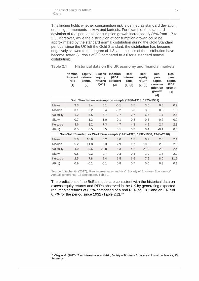
Over time the distribution of consumption outcomes in the UK has become more volatile and more negatively skewed. Risk of the UK economy measured by either consumption growth or GDP growth increased over the period 1718–2016 (Table 2.1). More precisely, the distribution of economic outcomes was more dispersed during the periods when the UK was off the Gold Standard compared with when it was on the Gold Standard.
28 Sharpe, W. (1964), ‘Capital Asset Prices: A Theory of Market Equilibrium under Conditions of Risk’, The Journal of Finance, 19: 3, September, pp. 433–34. 29 The ERP (observed excess equity returns), RFR, and volatility of equity returns have been respectively higher, lower, and higher than predicted by traditional finance theory. 30 Rietz, T.A. (1988), ‘The Equity Risk Premium: A Solution’, Journal of Monetary Economics, 22, July, pp. 91–115; Barro, R.J. (2009), ‘Rare Disasters, Asset Prices, and Welfare Costs’, American Economic Review, 99:1, pp. 243–64. 31 Martin, I. (2013), ‘Consumption-Based Asset Pricing with Higher Cumulants’, Review of Economic Studies, 80, pp. 746. 32 Specifically, Epstein-Zin preferences are used. This allows for the elasticity of intertemporal substitution and risk aversion to be independent of each other rather than jointly determined, as in the standard CAPM. 33 Summarised in Vlieghe, G. (2017), ‘Real interest rates and risk’, Society of Business Economists' Annual conference, 15 September. 34 Martin, I. (2013), ‘Consumption-Based Asset Pricing with Higher Cumulants’, Review of Economic Studies, 80, pp. 750–51.
The cost of equity for RIIO-2 Oxera
17
This finding holds whether consumption risk is defined as standard deviation, or as higher moments—skew and kurtosis. For example, the standard deviation of real per capita consumption growth increased by 35% from 1.7 to 2.3. Moreover, while the distribution of consumption growth could be approximated by the standard normal distribution during the Gold Standard periods, since the UK left the Gold Standard, the distribution has become negatively skewed to the degree of 1.3, and the tails of the distribution have become ‘fatter’ (kurtosis of 8.0 compared to 3.0 for a standard normal distribution).
Table 2.1 Historical data on the UK economy and financial markets
Nominal interest
rate
(1)
Equity returns (annual)
(2)
Excess equity returns (2)-(1)
Inflation (GDP
deflator)
(3)
Real interest
rate
(1)-(3)
Real equity return
(2)-(3)
Real per-
capita consumption on growth
(4)
Real per-
capita GDP
growth
(4)
Gold Standard—consumption sample (1830–1913, 1925–1931)
Mean 3.3 3.4 0.1 -0.1 3.5 3.6 0.8 0.9
Median 3.1 3.2 0.4 -0.2 3.3 3.5 0.8 1.3
Volatility 1.2 5.5 5.7 2.7 2.7 6.6 1.7 2.5
Skew 0.7 -1.2 -1.0 0.1 0.3 -0.5 -0.2 -0.2
Kurtosis 3.6 8.2 7.3 4.7 4.3 4.9 2.4 2.8
AR(1) 0.5 0.5 0.5 0.1 0.2 0.4 -0.1 0.0
Non-Gold Standard or World War sample (1921–1925, 1932–1938, 1948–2016)
Mean 5.6 10.8 5.2 4.0 1.6 6.9 2.0 2.1
Median 5.2 11.8 8.3 2.9 1.7 10.5 2.3 2.3
Volatility 4.0 20.6 20.8 5.3 4.2 21.0 2.3 2.4
Skew 0.5 -0.3 -0.7 0.3 0.4 -1.0 -1.3 -2.2
Kurtosis 2.5 7.8 8.4 6.5 6.6 7.6 8.0 11.5
AR(1) 0.9 -0.1 -0.1 0.8 0.7 0.0 0.3 0.1
Source: Vlieghe, G. (2017), ‘Real interest rates and risk’, Society of Business Economists' Annual conference, 15 September, Table 1.
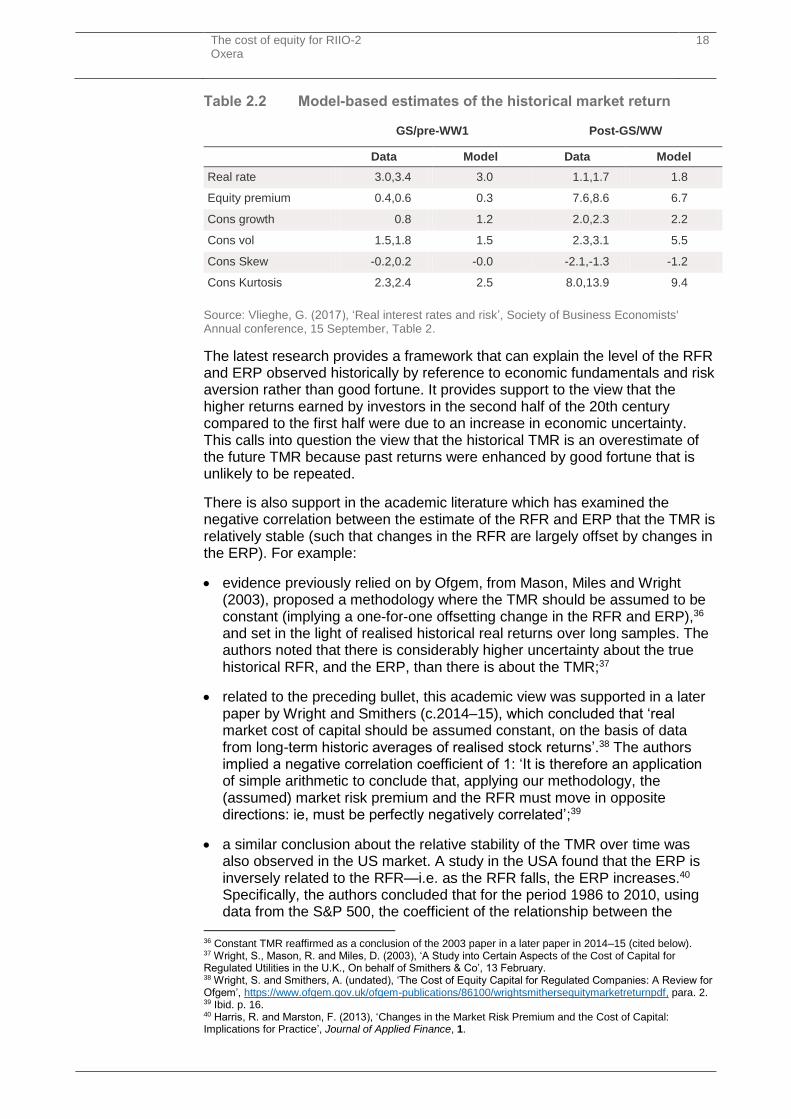
The predictions of the BoE’s model are consistent with the historical data on excess equity returns and RFRs observed in the UK by generating expected real market returns of 8.5% comprised of a real RFR of 1.8% and an ERP of 6.7% for the period since 1932 (Table 2.2).35
35 Vlieghe, G. (2017), ‘Real interest rates and risk’, Society of Business Economists' Annual conference, 15 September.
The cost of equity for RIIO-2 Oxera
18
Table 2.2 Model-based estimates of the historical market return
GS/pre-WW1 Post-GS/WW
Data Model Data Model
Real rate 3.0,3.4 3.0 1.1,1.7 1.8
Equity premium 0.4,0.6 0.3 7.6,8.6 6.7
Cons growth 0.8 1.2 2.0,2.3 2.2
Cons vol 1.5,1.8 1.5 2.3,3.1 5.5
Cons Skew -0.2,0.2 -0.0 -2.1,-1.3 -1.2
Cons Kurtosis 2.3,2.4 2.5 8.0,13.9 9.4
Source: Vlieghe, G. (2017), ‘Real interest rates and risk’, Society of Business Economists' Annual conference, 15 September, Table 2.
The latest research provides a framework that can explain the level of the RFR and ERP observed historically by reference to economic fundamentals and risk aversion rather than good fortune. It provides support to the view that the higher returns earned by investors in the second half of the 20th century compared to the first half were due to an increase in economic uncertainty. This calls into question the view that the historical TMR is an overestimate of the future TMR because past returns were enhanced by good fortune that is unlikely to be repeated.
There is also support in the academic literature which has examined the negative correlation between the estimate of the RFR and ERP that the TMR is relatively stable (such that changes in the RFR are largely offset by changes in the ERP). For example:
evidence previously relied on by Ofgem, from Mason, Miles and Wright (2003), proposed a methodology where the TMR should be assumed to be constant (implying a one-for-one offsetting change in the RFR and ERP),36 and set in the light of realised historical real returns over long samples. The authors noted that there is considerably higher uncertainty about the true historical RFR, and the ERP, than there is about the TMR;37
related to the preceding bullet, this academic view was supported in a later paper by Wright and Smithers (c.2014–15), which concluded that ‘real market cost of capital should be assumed constant, on the basis of data from long-term historic averages of realised stock returns’.38 The authors implied a negative correlation coefficient of 1: ‘It is therefore an application of simple arithmetic to conclude that, applying our methodology, the (assumed) market risk premium and the RFR must move in opposite directions: ie, must be perfectly negatively correlated’;39
a similar conclusion about the relative stability of the TMR over time was also observed in the US market. A study in the USA found that the ERP is inversely related to the RFR—i.e. as the RFR falls, the ERP increases.40 Specifically, the authors concluded that for the period 1986 to 2010, using data from the S&P 500, the coefficient of the relationship between the
36 Constant TMR reaffirmed as a conclusion of the 2003 paper in a later paper in 2014–15 (cited below). 37 Wright, S., Mason, R. and Miles, D. (2003), ‘A Study into Certain Aspects of the Cost of Capital for Regulated Utilities in the U.K., On behalf of Smithers & Co’, 13 February. 38 Wright, S. and Smithers, A. (undated), ‘The Cost of Equity Capital for Regulated Companies: A Review for Ofgem’, https://www.ofgem.gov.uk/ofgem-publications/86100/wrightsmithersequitymarketreturnpdf, para. 2. 39 Ibid. p. 16. 40 Harris, R. and Marston, F. (2013), ‘Changes in the Market Risk Premium and the Cost of Capital: Implications for Practice’, Journal of Applied Finance, 1.
The cost of equity for RIIO-2 Oxera
19
interest rate and the ERP was -0.79, such that a 1% decline in the RFR would be offset by a 0.79% increase in the ERP.41
Overall, the latest asset pricing research refutes the view that the ERP is a stable parameter and that the main source of variation over time in the TMR is the RFR.
2.2.2 Historical data
The latest estimate of the average of UK real equity returns over the period 1900–2016 is 5.5–7.3%.42 The lower bound of this range is the geometric average of the historical data and the upper bound is the arithmetic average. In light of the evidence presented in Box 2.1, it is appropriate to select an estimate close to the arithmetic average.
Box 2.1 Geometric versus arithmetic means
The geometric mean of any set of numbers is always lower than the arithmetic mean unless all the numbers are equal (in which case the means are the same). For a series of returns, equality between the geometric and arithmetic means would occur only if there is no volatility at all (i.e. if returns are constant). While there is debate about which is the more appropriate averaging method in any given context, the academic literature is broadly supportive of placing more weight on the arithmetic averages for estimating the ERP to use when computing required equity returns. Indeed, DMS themselves write:43
This [the arithmetic mean risk premium] is our estimate of the expected long-run equity risk premium for use in asset allocation, stock valuation, and corporate budgeting applications.
This is consistent with a number of analytical studies that suggest that greater weight should be placed on arithmetic than on geometric estimates of returns.44 Cooper (1996) analyses the properties of three approximately unbiased estimators of expected returns from the academic literature, and notes:
The use of the arithmetic mean ignores estimation error and serial correlation in returns. Unbiased discount factors have been derived that correct for both these effects. In all cases, the corrected discount rates are closer to the arithmetic than the geometric mean.45
and that:
the geometric mean is a significantly downward biased estimate of discount rates even when ‘market overreaction’ is taken into account.46
This conclusion is further supported by Jacquier, Kane and Marcus (2003), who derive a relatively simple formula for a correct estimator for the
41 Harris, R. and Marston, F. (2013), ‘Changes in the Market Risk Premium and the Cost of Capital: Implications for Practice’, Journal of Applied Finance, 1, pp. 6–7. 42 Dimson, E., Marsh, P. and Staunton, M. (2017), 'Credit Suisse Global Investment Returns Yearbook 2017', p. 14. 43 Dimson, E., Marsh, P. and Staunton, M. (2015), ‘Credit Suisse Investment Returns Sourcebook 2015’, p. 34. 44 For further details, see Cooper, I. (1996), ‘Arithmetic versus geometric mean estimators: Setting discount rates for capital budgeting’, European Financial Management, 2:2, p. 157. 45 Ibid. 46 Ibid., p. 165.
The cost of equity for RIIO-2 Oxera
20
expected future ERP.47 The authors suggest a weighted average between the arithmetic and geometric means, with the weight on the geometric mean being the ratio of the investment horizon to the sample period. This means that, for short investment horizons, the best estimator is very close to the arithmetic mean, whereas for long investment horizons the weight of the geometric mean increases.
In our case, the sample period is 116 years, since the DMS database contains 116 years of data. If RIIO-2 will be the same duration as RIIO-1, the weight on the geometric mean would be 8/116 = 7%. For a shorter price control period, the weight on the geometric mean would be even smaller.
The estimator by Jacquier, Kane and Marcus (2003) has been used in regulatory discussions—for example, in the Competition Commission (CC) referrals concerning Bristol Water,48 and NIE.49
The revisions to the calculation of the RPI inflation statistic made by the Office for National Statistics (ONS) in 2010 created a structural increase in the RPI measure of inflation.50 All else equal, this would make the historical real equity market returns an upwardly biased estimate of the future TMR calculated relative to RPI. However, there are likely to have been other revisions to the calculation of RPI during the 116-year history of the UK equity returns dataset, some of which may have introduced a downward bias to average historical real equity market returns. For example, in 2015, the OBR stated that its estimate of the long-run wedge between RPI and CPI would be reduced by about 40bp.51 A comprehensive examination of the historical inflation data would be needed before concluding that the 2010 revision to the RPI calculation has made the historical real equity market returns an upwardly biased estimate of the future TMR.
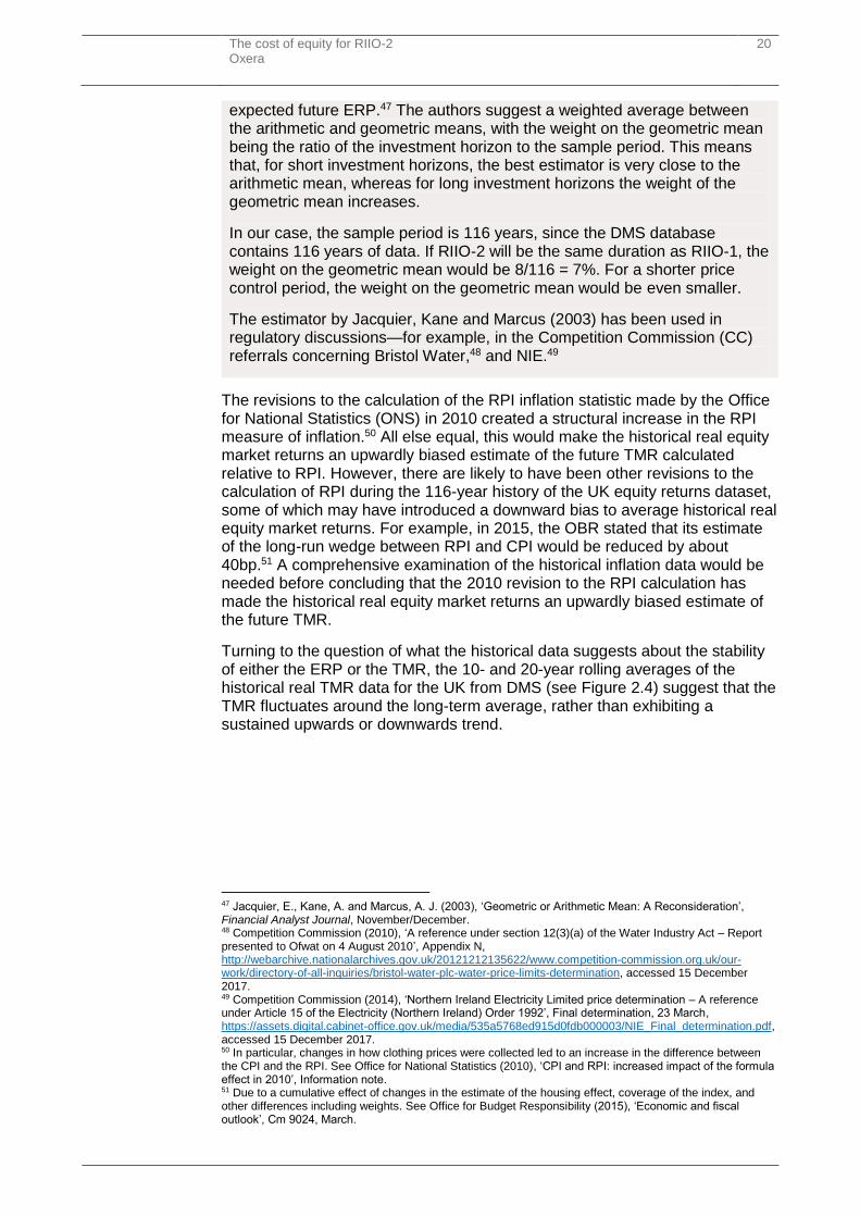
Turning to the question of what the historical data suggests about the stability of either the ERP or the TMR, the 10- and 20-year rolling averages of the historical real TMR data for the UK from DMS (see Figure 2.4) suggest that the TMR fluctuates around the long-term average, rather than exhibiting a sustained upwards or downwards trend.
47 Jacquier, E., Kane, A. and Marcus, A. J. (2003), ‘Geometric or Arithmetic Mean: A Reconsideration’, Financial Analyst Journal, November/December. 48 Competition Commission (2010), ‘A reference under section 12(3)(a) of the Water Industry Act – Report presented to Ofwat on 4 August 2010’, Appendix N, http://webarchive.nationalarchives.gov.uk/20121212135622/www.competition-commission.org.uk/our-work/directory-of-all-inquiries/bristol-water-plc-water-price-limits-determination, accessed 15 December 2017. 49 Competition Commission (2014), ‘Northern Ireland Electricity Limited price determination – A reference under Article 15 of the Electricity (Northern Ireland) Order 1992’, Final determination, 23 March, https://assets.digital.cabinet-office.gov.uk/media/535a5768ed915d0fdb000003/NIE_Final_determination.pdf, accessed 15 December 2017. 50 In particular, changes in how clothing prices were collected led to an increase in the difference between the CPI and the RPI. See Office for National Statistics (2010), ‘CPI and RPI: increased impact of the formula effect in 2010’, Information note. 51 Due to a cumulative effect of changes in the estimate of the housing effect, coverage of the index, and other differences including weights. See Office for Budget Responsibility (2015), ‘Economic and fiscal outlook’, Cm 9024, March.
The cost of equity for RIIO-2 Oxera
21
Figure 2.4 UK real TMR, 1900–2016
Source: Oxera analysis based on Dimson et al. (2017), op. cit.
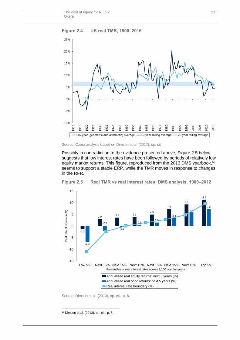
Possibly in contradiction to the evidence presented above, Figure 2.5 below suggests that low interest rates have been followed by periods of relatively low equity market returns. This figure, reproduced from the 2013 DMS yearbook,52 seems to support a stable ERP, while the TMR moves in response to changes in the RFR.
Figure 2.5 Real TMR vs real interest rates: DMS analysis, 1900–2012
Source: Dimson et al. (2013), op. cit., p. 8.
52 Dimson et al. (2013), op. cit., p. 8.
-10%
-5%
0%
5%
10%
15%
20%
25%
1910
1915
1920
1925
1930
1935
1940
1945
1950
1955
1960
1965
1970
1975
1980
1985
1990
1995
2000
2005
2010
2015
116-year (geometric and arithmetic) average 10-year rolling average 20-year rolling average
-1.2
3.03.6 3.9
4.9
7.3
9.3
11.3
-6.8
-2.0
-0.5
0.51.5
3.4
5.9
7.2
-11
-2.3
0.1
1.5
2.8
4.8
9.6
-15
-10
-5
0
5
10
15
Low 5% Next 15% Next 15% Next 15% Next 15% Next 15% Next 15% Top 5%
Re
al ra
te o
f re
turn
(in
%)
Percentiles of real interest rates across 2,160 country-years
Annualised real equity returns: next 5 years (%)
Annualised real bond returns: next 5 years (%)
Real interest rate boundary (%)
The cost of equity for RIIO-2 Oxera
22
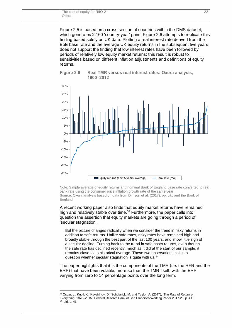
Figure 2.5 is based on a cross-section of countries within the DMS dataset, which generates 2,160 ‘country-year’ pairs. Figure 2.6 attempts to replicate this finding based solely on UK data. Plotting a real interest rate derived from the BoE base rate and the average UK equity returns in the subsequent five years does not support the finding that low interest rates have been followed by periods of relatively low equity market returns; this result is robust to sensitivities based on different inflation adjustments and definitions of equity returns.
Figure 2.6 Real TMR versus real interest rates: Oxera analysis, 1900–2012
Note: Simple average of equity returns and nominal Bank of England base rate converted to real bank rate using the consumer price inflation growth rate of the same year. Source: Oxera analysis based on data from Dimson et al. (2017), op. cit., and the Bank of England.
A recent working paper also finds that equity market returns have remained high and relatively stable over time.53 Furthermore, the paper calls into question the assertion that equity markets are going through a period of ‘secular stagnation’.
But the picture changes radically when we consider the trend in risky returns in addition to safe returns. Unlike safe rates, risky rates have remained high and broadly stable through the best part of the last 100 years, and show little sign of a secular decline. Turning back to the trend in safe asset returns, even though the safe rate has declined recently, much as it did at the start of our sample, it remains close to its historical average. These two observations call into question whether secular stagnation is quite with us.54
The paper highlights that it is the components of the TMR (i.e. the RFR and the ERP) that have been volatile, more so than the TMR itself, with the ERP varying from zero to 14 percentage points over the long term.
53 Òscar, J., Knoll, K., Kuvshinov, D., Schularick, M. and Taylor, A. (2017), ‘The Rate of Return on Everything, 1870–2015’, Federal Reserve Bank of San Francisco Working Paper 2017-25, p. 41. 54 Ibid. p. 41.
-25%
-20%
-15%
-10%
-5%
0%
5%
10%
15%
20%
25%
30%
Equity returns (next 5 years, average) Bank rate (real)
The cost of equity for RIIO-2 Oxera
23
We now turn to examine the long-run developments in the risk premium, i.e. the spread between safe and risky returns. This spread was low and stable at around 5 percentage points before WW1. It rose slightly after the WW1, before falling to an all-time low of near zero by around 1930. The decades following the onset of the WW2 saw a dramatic widening in the risk premium, with the spread reaching its historical high of around 14 percentage points in the 1950s, before falling back to around its historical average.55
On balance, evidence from historical data supports the view that the expected TMR is broadly stable and that changes in the RFR are largely offset by changes in the ERP.
2.2.3 Survey evidence
Another source of evidence for the ERP and TMR is surveys. Survey evidence needs to be interpreted with caution, however. Issues with interpretation of survey evidence include the following:
respondents’ answers may be influenced by the way questions are phrased—for example, whether the question asks about required returns to equity or expected returns on a specified stock market index;
there is a tendency for respondents to extrapolate from recent realised returns, making the estimates less forward-looking and prone to be anchored on recent short-term market performance;
the results are based purely on judgement, which may also be influenced by the respondent’s own position or biases, and are less reliable than estimates based on direct market evidence on pricing.
As stated by Brealey and Myers (2017):
Do not trust anyone who claims to know what returns investors expect. History contains some clues, but ultimately we have to judge whether investors on average have received what they expected.56
Notwithstanding the need to interpret the survey evidence with caution, this sub-section presents evidence in relation to respondents’ expectations about ERP and TMR. First, Figure 2.7 shows TMR survey evidence for the USA, based on a quarterly survey of Chief Financial Officers in the USA conducted by Duke University and the CFO Magazine. Among other questions, the CFOs were asked about their view of the long-term expected return on the S&P 500.
55 Ibid. p. 42. 56 Brealey, R., Myers, S., Allen F. (2016), Principles of Corporate Finance, 12th edition, McGraw-Hill International Edition, p. 169.
The cost of equity for RIIO-2 Oxera
24
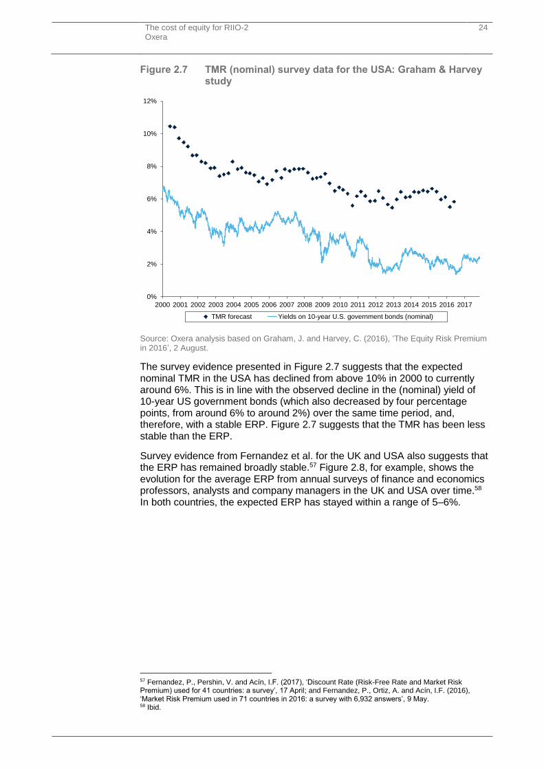
Figure 2.7 TMR (nominal) survey data for the USA: Graham & Harvey study
Source: Oxera analysis based on Graham, J. and Harvey, C. (2016), ‘The Equity Risk Premium in 2016’, 2 August.
The survey evidence presented in Figure 2.7 suggests that the expected nominal TMR in the USA has declined from above 10% in 2000 to currently around 6%. This is in line with the observed decline in the (nominal) yield of 10-year US government bonds (which also decreased by four percentage points, from around 6% to around 2%) over the same time period, and, therefore, with a stable ERP. Figure 2.7 suggests that the TMR has been less stable than the ERP.
Survey evidence from Fernandez et al. for the UK and USA also suggests that the ERP has remained broadly stable.57 Figure 2.8, for example, shows the evolution for the average ERP from annual surveys of finance and economics professors, analysts and company managers in the UK and USA over time.58 In both countries, the expected ERP has stayed within a range of 5–6%.
57 Fernandez, P., Pershin, V. and Acín, I.F. (2017), ‘Discount Rate (Risk-Free Rate and Market Risk Premium) used for 41 countries: a survey’, 17 April; and Fernandez, P., Ortiz, A. and Acín, I.F. (2016), ‘Market Risk Premium used in 71 countries in 2016: a survey with 6,932 answers’, 9 May. 58 Ibid.
0%
2%
4%
6%
8%
10%
12%
2000 2001 2002 2003 2004 2005 2006 2007 2008 2009 2010 2011 2012 2013 2014 2015 2016 2017
TMR forecast Yields on 10-year U.S. government bonds (nominal)

The cost of equity for RIIO-2 Oxera
25
Figure 2.8 ERP survey data from Fernandez et al. for the UK and USA
Source: Oxera analysis based on Fernandez et al. (2017), op. cit., and (2016), op. cit.
Overall, the evidence from surveys seems to support the first view—that the ERP is approximately constant over time and largely independent of the RFR.
2.2.4 Discount rates used by infrastructure funds
The discount rates used by infrastructure funds to value their portfolios may provide another source of evidence for the TMR and ERP. Figure 2.9 shows the nominal discount rate used by 3i Infrastructure plc for its portfolio of infrastructure equity investments over time.
Figure 2.9 3i Infrastructure portfolio-weighted average discount rate
Source: Oxera analysis based on RBC Capital Markets (2017), ‘3i Infrastructure plc–Solid 7.1% return and cash generation in 1H18’, 9 November, p. 2.
5.3%5.5% 5.5%
5.1% 5.2% 5.3%
5.9%
5.5% 5.5%5.7%
5.4% 5.5%5.3%
5.7%
0%
1%
2%
3%
4%
5%
6%
7%
2011 2012 2013 2014 2015 2016 2017
United Kingdom USA
12.4%
13.8%
12.5%
13.2%12.6%
12.0% 11.8%10.9%
10.2%
9.9%
10.1%10.0%
10.0%
0.0%
2.0%
4.0%
6.0%
8.0%
10.0%
12.0%
14.0%
16.0%
Mar-
08
Sep-0
8
Mar-
09
Sep-0
9
Mar-
10
Sep-1
0
Mar-
11
Sep-1
1
Mar-
12
Sep-1
2
Mar-
13
Sep-1
3
Mar-
14
Sep-1
4
Mar-
15
Sep-1
5
Mar-
16
Sep-1
6
Mar-
17
Sep-1
7
Discount rate
The cost of equity for RIIO-2 Oxera
26
The decrease in the discount rate over time is broadly in line with the decrease in the real RFR over the same time period. This supports the view that the ERP is stable, but may also be driven by changes in the mix of assets and the equity risk of the portfolio (i.e. the equity beta).
Removing 3% RPI inflation from the current nominal portfolio discount rate of 10.0% yields a real discount rate of around 7% cost of equity for infrastructure. The implied TMR would also be around 7%, assuming an equity beta close to one.
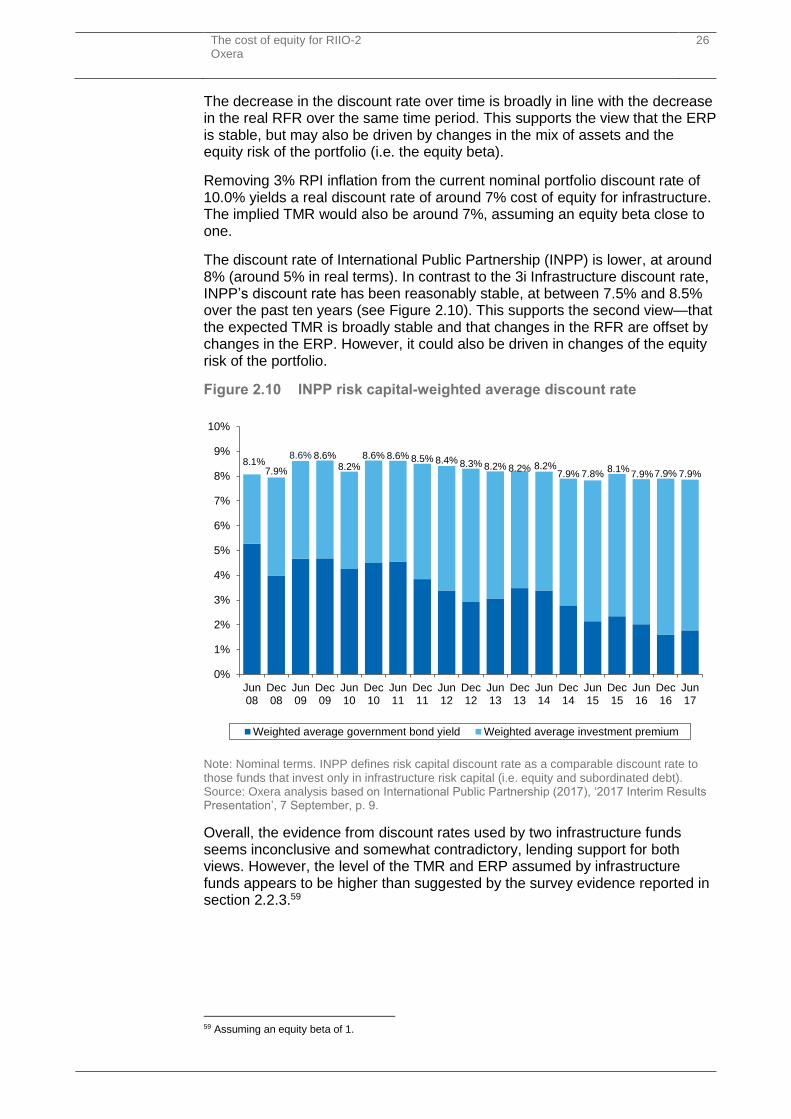
The discount rate of International Public Partnership (INPP) is lower, at around 8% (around 5% in real terms). In contrast to the 3i Infrastructure discount rate, INPP’s discount rate has been reasonably stable, at between 7.5% and 8.5% over the past ten years (see Figure 2.10). This supports the second view—that the expected TMR is broadly stable and that changes in the RFR are offset by changes in the ERP. However, it could also be driven in changes of the equity risk of the portfolio.
Figure 2.10 INPP risk capital-weighted average discount rate
Note: Nominal terms. INPP defines risk capital discount rate as a comparable discount rate to those funds that invest only in infrastructure risk capital (i.e. equity and subordinated debt). Source: Oxera analysis based on International Public Partnership (2017), ‘2017 Interim Results Presentation’, 7 September, p. 9.
Overall, the evidence from discount rates used by two infrastructure funds seems inconclusive and somewhat contradictory, lending support for both views. However, the level of the TMR and ERP assumed by infrastructure funds appears to be higher than suggested by the survey evidence reported in section 2.2.3.59
59 Assuming an equity beta of 1.
8.1%7.9%
8.6% 8.6%8.2%
8.6% 8.6% 8.5% 8.4% 8.3% 8.2% 8.2% 8.2%7.9% 7.8%
8.1%7.9%7.9% 7.9%
0%
1%
2%
3%
4%
5%
6%
7%
8%
9%
10%
Jun08
Dec08
Jun09
Dec09
Jun10
Dec10
Jun11
Dec11
Jun12
Dec12
Jun13
Dec13
Jun14
Dec14
Jun15
Dec15
Jun16
Dec16
Jun17
Weighted average government bond yield Weighted average investment premium
The cost of equity for RIIO-2 Oxera
27
2.2.5 Variants of the dividend discount model
The BoE regularly estimates the ERP based on a DDM.60 The BoE has suggested that ERPs are facing upward pressure based on estimates derived from the DDM:
The Bank’s calculations show that the equity risk premium (ERP) may have roughly doubled from its perhaps unsustainably low level at the turn of the century during the dot-com boom. This rise in the ERP has been working vigorously against the fall in the risk-free rate…Members of the Bank’s Monetary Policy Committee have argued that interest rates are as low as they are not because of coordinated central bank whim but because there is so much caution in the system…People seem to think some catastrophic outcome is possible, and this in turn pushes up the ERP. Whatever is going on, it hangs over the economy as well as the banks, and it should not be underestimated.61
As mentioned in section 2.2.1, asset pricing models that incorporate the potential for catastrophic (i.e. negatively skewed) economic outcomes or less restrictive assumptions about the preferences of consumers and investors will generate a higher ERP. This provides a theoretical basis for the ERP estimates implied by the DDM.
In the DDM, the expected TMR is the discount rate at which the present value of future dividends is equal to the current market price of the shares. In the context of estimating the return for the whole UK equity market, data on the FTSE All-share index is typically used.
Oxera has constructed a DDM following the BoE methodology. The outputs from the Oxera model closely match those reported by the BoE: the ERP calculated from the model for February 2017 is 8.9% compared with approximately 9.0% reported by the BoE.62 This estimate is 400bp higher than the historical arithmetic average excess equity return reported by DMS, consistent with the view that changes in the RFR are largely offset by changes in the ERP.
It is not possible to infer the TMR directly from the ERP estimates published by the BoE because the BoE uses multiple interest rates across the whole yield curve. However, the Oxera model enables a TMR to be calculated that is internally consistent with the BoE methodology. Figure 2.11 presents the TMR estimates since 2004, which are volatile over time but appear to revert to a longer-term average; whereas the ERP estimates appear more volatile. The figure also shows that the expected TMR is not currently abnormally low and has not followed the downward trend in interest rates over this period.
60 The BoE regularly published ERP estimates in its Financial Stability Reports based on the DDM outlined in Inkinen, M., Stringa, M. and Voutsinou, K. (2010), ‘Interpreting equity price movements since the start of the financial crisis’, Bank of England Quarterly Bulletin, 50:1, p. 24–33. This model has recently been improved in Dison, W. and Rattan, A. (2017), ‘An improved model for understanding equity prices’, Quarterly Bulletin 2017 Q2. 61 Taylor, M. (2016), ‘Banking in the Tundra’, speech by Martin Taylor, External Member of the Financial Policy Committee, Bank of England, Official Monetary and Financial Institutions Forum City Lecture, London, 25 May. 62 Dison and Rattan (2017), op. cit.
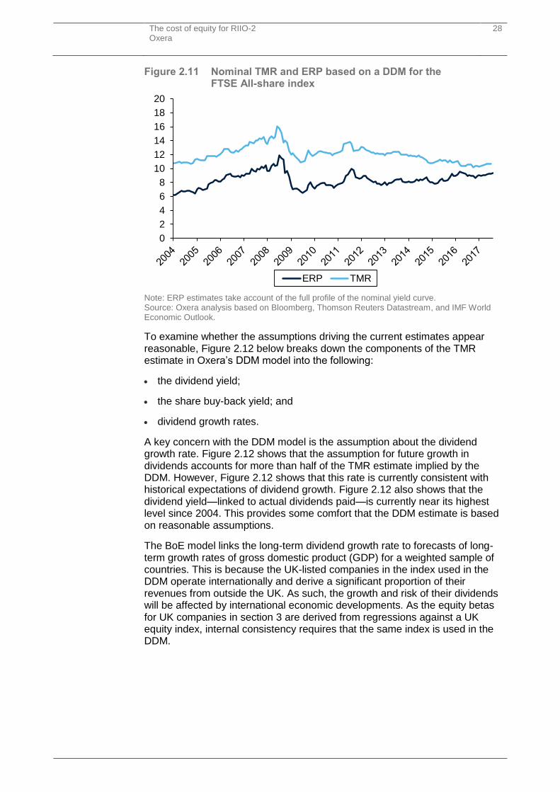
The cost of equity for RIIO-2 Oxera
28
Figure 2.11 Nominal TMR and ERP based on a DDM for the FTSE All-share index
Note: ERP estimates take account of the full profile of the nominal yield curve. Source: Oxera analysis based on Bloomberg, Thomson Reuters Datastream, and IMF World Economic Outlook.
To examine whether the assumptions driving the current estimates appear reasonable, Figure 2.12 below breaks down the components of the TMR estimate in Oxera’s DDM model into the following:
the dividend yield;
the share buy-back yield; and
dividend growth rates.
A key concern with the DDM model is the assumption about the dividend growth rate. Figure 2.12 shows that the assumption for future growth in dividends accounts for more than half of the TMR estimate implied by the DDM. However, Figure 2.12 shows that this rate is currently consistent with historical expectations of dividend growth. Figure 2.12 also shows that the dividend yield—linked to actual dividends paid—is currently near its highest level since 2004. This provides some comfort that the DDM estimate is based on reasonable assumptions.
The BoE model links the long-term dividend growth rate to forecasts of long-term growth rates of gross domestic product (GDP) for a weighted sample of countries. This is because the UK-listed companies in the index used in the DDM operate internationally and derive a significant proportion of their revenues from outside the UK. As such, the growth and risk of their dividends will be affected by international economic developments. As the equity betas for UK companies in section 3 are derived from regressions against a UK equity index, internal consistency requires that the same index is used in the DDM.
0
2
4
6
8
10
12
14
16
18
20
ERP TMR
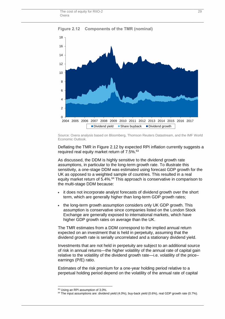
The cost of equity for RIIO-2 Oxera
29
Figure 2.12 Components of the TMR (nominal)
Source: Oxera analysis based on Bloomberg, Thomson Reuters Datastream, and the IMF World Economic Outlook.
Deflating the TMR in Figure 2.12 by expected RPI inflation currently suggests a required real equity market return of 7.5%.63
As discussed, the DDM is highly sensitive to the dividend growth rate assumptions, in particular to the long-term growth rate. To illustrate this sensitivity, a one-stage DDM was estimated using forecast GDP growth for the UK as opposed to a weighted sample of countries. This resulted in a real equity market return of 5.4%.64 This approach is conservative in comparison to the multi-stage DDM because:
it does not incorporate analyst forecasts of dividend growth over the short term, which are generally higher than long-term GDP growth rates;
the long-term growth assumption considers only UK GDP growth. This assumption is conservative since companies listed on the London Stock Exchange are generally exposed to international markets, which have higher GDP growth rates on average than the UK.
The TMR estimates from a DDM correspond to the implied annual return expected on an investment that is held in perpetuity, assuming that the dividend growth rate is serially uncorrelated and a stationary dividend yield.
Investments that are not held in perpetuity are subject to an additional source of risk in annual returns—the higher volatility of the annual rate of capital gain relative to the volatility of the dividend growth rate—i.e. volatility of the price–earnings (P/E) ratio.
Estimates of the risk premium for a one-year holding period relative to a perpetual holding period depend on the volatility of the annual rate of capital
63 Using an RPI assumption of 3.0%. 64 The input assumptions are: dividend yield (4.0%), buy-back yield (0.6%), real GDP growth rate (0.7%).
0
2
4
6
8
10
12
14
16
18
2004 2005 2006 2007 2008 2009 2010 2011 2012 2013 2014 2015 2016 2017
Dividend yield Share buyback Dividend growth
The cost of equity for RIIO-2 Oxera
30
gain relative to the volatility of the dividend growth rate. Fama–French (2002) estimated this adjustment to be 130bp based on US data.65
Investors in energy networks would be expected to have investment horizons longer than one year. On this basis, some increase to DDM-based estimates of the TMR to account for P/E ratio volatility appears appropriate.
Overall, the evidence from the DDM is consistent with the view that the TMR is a relatively stable parameter over time, and that changes in the ERP largely offset changes in the RFR.
2.2.6 Vector autoregression model
An alternative to the DDM discussed in the previous section for estimating expected equity returns is the vector autoregression (VAR) model.66 This statistical model predicts future long-term equity returns based on the relationship between short-term returns and other explanatory variables.
A recent working paper published by the BoE examined the predictive power of the estimates from DDMs and VAR models using a variety of tests. It finds that the estimated return measures from both models ‘can significantly forecast returns.’67 ‘Out-of-sample, the VAR and DDM estimates generate economically and statistically significant forecast improvements relative to a historical average benchmark.’68
Furthermore, the authors find that ‘the VAR-based estimate generates substantially lower forecast errors compared to the DDM estimate’ 69 and that the results ‘tentatively suggest that the VAR approach better captures expected returns compared to the DDM’.70 The BoE draws this conclusion based on application to both US and UK data, and the model fits the US data better than the UK data.
The estimated nominal TMR for the UK based on the VAR model, shown in Figure 2.13, was around 14% in 2013. Using an RPI inflation rate of 3%, a nominal TMR of 14% corresponds to a real TMR of around 11%. This is significantly higher than estimates based on the DDM presented in the previous section.
65 Fama, E. and French, K. (2002), ‘The Equity Premium’, The Journal of Finance, LVII:2, pp. 654–57. 66 Based on Campbell, J.Y. (1991), ‘A Variance Decomposition for Stock Returns’, The Economic Journal, 101:405, pp. 157–79. 67 Chin, M. and Polk, C. (2015), ‘A forecast evaluation of expected equity return measures’, Bank of England Working Paper No. 520, January, p. 24. 68 Ibid., p. 1. 69 Ibid., p. 24. 70 Ibid., p. 1.
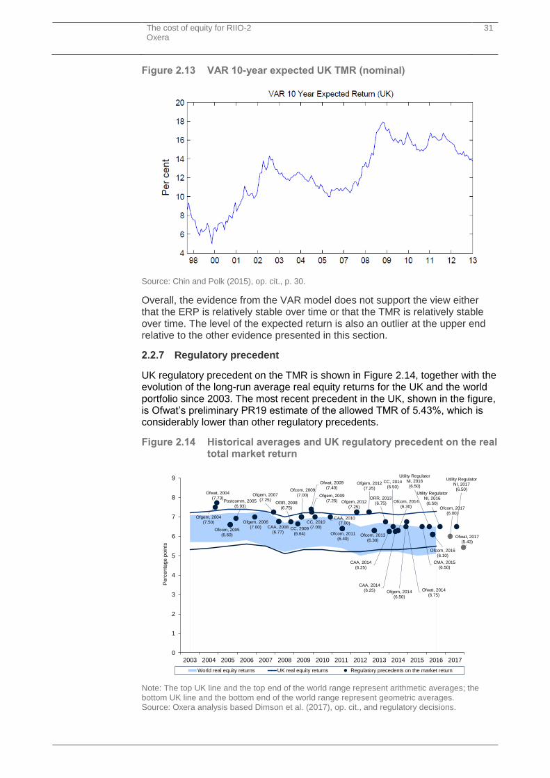
The cost of equity for RIIO-2 Oxera
31
Figure 2.13 VAR 10-year expected UK TMR (nominal)
Source: Chin and Polk (2015), op. cit., p. 30.
Overall, the evidence from the VAR model does not support the view either that the ERP is relatively stable over time or that the TMR is relatively stable over time. The level of the expected return is also an outlier at the upper end relative to the other evidence presented in this section.
2.2.7 Regulatory precedent
UK regulatory precedent on the TMR is shown in Figure 2.14, together with the evolution of the long-run average real equity returns for the UK and the world portfolio since 2003. The most recent precedent in the UK, shown in the figure, is Ofwat’s preliminary PR19 estimate of the allowed TMR of 5.43%, which is considerably lower than other regulatory precedents.
Figure 2.14 Historical averages and UK regulatory precedent on the real total market return
Note: The top UK line and the top end of the world range represent arithmetic averages; the bottom UK line and the bottom end of the world range represent geometric averages. Source: Oxera analysis based Dimson et al. (2017), op. cit., and regulatory decisions.
Ofwat, 2004(7.73)
Ofgem, 2004(7.50)
Postcomm, 2005(6.93)
Ofcom, 2005(6.60)
Ofgem, 2006(7.00)
Ofgem, 2007(7.25)
ORR, 2008(6.75)
CAA, 2008(6.77)
Ofcom, 2009(7.00)
CC, 2009(6.64)
Ofwat, 2009(7.40)
Ofgem, 2009(7.25)
CC, 2010(7.00)
CAA, 2010(7.00)
Ofcom, 2011(6.40)
Ofgem, 2012(7.25)
Ofgem, 2012(7.25)
Ofcom, 2013(6.30)
ORR, 2013(6.75)
CAA, 2014(6.25)
CC, 2014(6.50)
Ofcom, 2014(6.30)
CAA, 2014(6.25) Ofgem, 2014
(6.50)
Ofwat, 2014(6.75)
CMA, 2015(6.50)
Utility Regulator NI, 2016
(6.50)
Ofcom, 2016(6.10)
Utility Regulator NI, 2016
(6.50)
Utility Regulator NI, 2017
(6.50)
Ofcom, 2017(6.00)
Ofwat, 2017(5.43)
01/01/2003 27/09/2005 23/06/2008 20/03/2011 14/12/2013 09/09/2016
0
1
2
3
4
5
6
7
8
9
2003 2004 2005 2006 2007 2008 2009 2010 2011 2012 2013 2014 2015 2016 2017
Pe
rcen
tage
po
ints
World real equity returns UK real equity returns Regulatory precedents on the market return
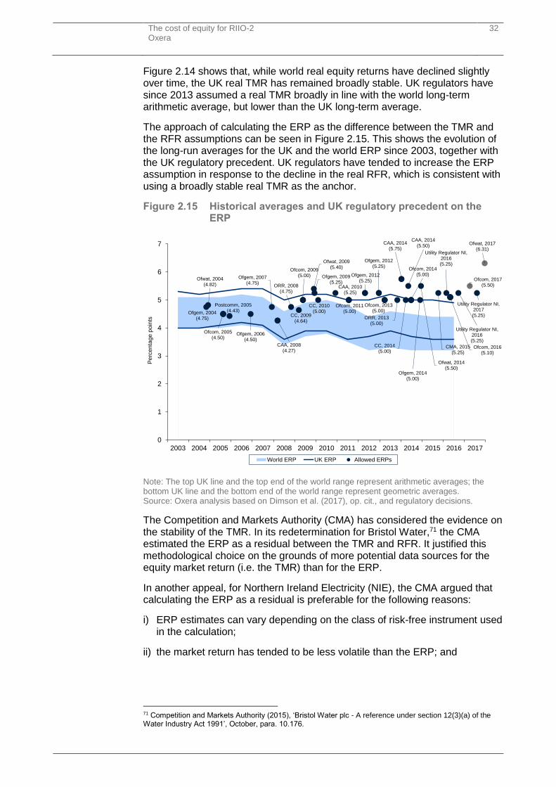
The cost of equity for RIIO-2 Oxera
32
Figure 2.14 shows that, while world real equity returns have declined slightly over time, the UK real TMR has remained broadly stable. UK regulators have since 2013 assumed a real TMR broadly in line with the world long-term arithmetic average, but lower than the UK long-term average.
The approach of calculating the ERP as the difference between the TMR and the RFR assumptions can be seen in Figure 2.15. This shows the evolution of the long-run averages for the UK and the world ERP since 2003, together with the UK regulatory precedent. UK regulators have tended to increase the ERP assumption in response to the decline in the real RFR, which is consistent with using a broadly stable real TMR as the anchor.
Figure 2.15 Historical averages and UK regulatory precedent on the ERP
Note: The top UK line and the top end of the world range represent arithmetic averages; the bottom UK line and the bottom end of the world range represent geometric averages. Source: Oxera analysis based on Dimson et al. (2017), op. cit., and regulatory decisions.
The Competition and Markets Authority (CMA) has considered the evidence on the stability of the TMR. In its redetermination for Bristol Water,71 the CMA estimated the ERP as a residual between the TMR and RFR. It justified this methodological choice on the grounds of more potential data sources for the equity market return (i.e. the TMR) than for the ERP.
In another appeal, for Northern Ireland Electricity (NIE), the CMA argued that calculating the ERP as a residual is preferable for the following reasons:
i) ERP estimates can vary depending on the class of risk-free instrument used in the calculation;
ii) the market return has tended to be less volatile than the ERP; and
71 Competition and Markets Authority (2015), ‘Bristol Water plc - A reference under section 12(3)(a) of the Water Industry Act 1991’, October, para. 10.176.
Ofwat, 2004(4.82)
Ofgem, 2004(4.75)
Postcomm, 2005(4.43)
Ofcom, 2005(4.50)
Ofgem, 2006(4.50)
Ofgem, 2007(4.75)
ORR, 2008(4.75)
CAA, 2008(4.27)
Ofcom, 2009(5.00)
CC, 2009(4.64)
Ofwat, 2009(5.40)
Ofgem, 2009(5.25)
CC, 2010(5.00)
CAA, 2010(5.25)
Ofcom, 2011(5.00)
Ofgem, 2012(5.25)
Ofgem, 2012(5.25)
Ofcom, 2013(5.00)
ORR, 2013(5.00)
CAA, 2014(5.75)
CC, 2014(5.00)
Ofcom, 2014(5.00)
CAA, 2014(5.50)
Ofgem, 2014(5.00)
Ofwat, 2014(5.50)
CMA, 2015(5.25)
Utility Regulator NI, 2016(5.25)
Ofcom, 2016(5.10)
Utility Regulator NI, 2016(5.25)
Utility Regulator NI, 2017(5.25)
Ofcom, 2017(5.50)
Ofwat, 2017(6.31)
01/01/2003 27/09/2005 23/06/2008 20/03/2011 14/12/2013 09/09/2016
0
1
2
3
4
5
6
7
2003 2004 2005 2006 2007 2008 2009 2010 2011 2012 2013 2014 2015 2016 2017
Pe
rce
nta
ge
po
ints
World ERP UK ERP Allowed ERPs

The cost of equity for RIIO-2 Oxera
33
iii) there is some evidence of the ERP being negatively correlated with Treasury bill rates over the short term.72
Overall, the CMA’s approach has been consistent with the view of a stable TMR—that the expected TMR reverts to a long-term average and that changes in the RFR are offset by changes in the ERP, at least in the short term.
2.3 Conclusion
As the start of RIIO-2 is over three years away, an initial estimate for the RFR (real, RPI-deflated) of -0.5 to 0.0% appears appropriate based on forward rates and allowing for volatility and uncertainty. We suggest that the evidence is monitored to ensure that it is incorporated into the final estimate of the cost of equity for RIIO-2, although it will still be necessary to allow for uncertainty regarding market developments during the RIIO-2 price control period.
We have assessed in this report that the estimation of the RFR cannot be considered in isolation from the ERP. A central conclusion of this report is that the RFR and ERP are negatively correlated, with the result that the TMR is more stable than the ERP alone.
Forming a precise view on the real expected TMR is made challenging by the wide range of estimates from the various sources of evidence. The central issue in the current debate over the TMR is the degree to which the expected ERP adjusts to offset changes in the RFR. The theoretical and empirical evidence basis for assuming a stable ERP appears weak. For example:
consumption-based asset pricing models find that higher economic uncertainty simultaneously places downward pressure on the RFR and upward pressure on the ERP;73
historical data shows that the RFR and ERP have been very volatile while total equity market returns have been relatively more stable over time, and calls into question the assertion that equity markets are going through a period of ‘secular stagnation’;74
estimates of the TMR from DDMs suggest that it is relatively stable over time and is currently no lower than its estimated value in the early 2000s.
The reliability of survey evidence and discount rate assumptions used by infrastructure funds is lower than more direct market evidence, but is inconclusive on whether the ERP or the TMR is the more stable parameter.
This suggests that an appropriate TMR assumption would place more weight on the view that the expected TMR is relatively stable, and close to its long-run average of 7.3%75, than the view that the ERP is close to its long-run average of 4.9% (implying a TMR of 4.4% when combined with forward interest rates, which are on average -0.5% for the RIIO-2 period).76
72 Competition Commission (2014), ‘Northern Ireland Electricity Limited; A reference under Article 15 of the Electricity (Northern Ireland) Order 1992’, 26 March, para. 13.82. 73 Martin, I. (2013), ‘Consumption-Based Asset Pricing with Higher Cumulants’, Review of Economic Studies, 80, pp. 746; Vlieghe, G. (2017), ‘Real interest rates and risk’, Society of Business Economists' Annual conference, 15 September. 74 Òscar, J., Knoll, K., Kuvshinov, D., Schularick, M., Taylor, A. (2017), ‘The Rate of Return on Everything, 1870–2015’, Federal Reserve Bank of San Francisco Working Paper 2017-25, p. 41. 75 Dimson, E., Marsh, P. and Staunton, M. (2017), 'Credit Suisse Global Investment Returns Yearbook 2017', p. 14. 76 Dimson et al. (2017), op. cit., p. 31.
The cost of equity for RIIO-2 Oxera
34
Attenuation of the upper end of the range—the version of the DDM used by the BoE indicates a real TMR of at least 7.5%, while the historical arithmetic average of the real TMR from Dimson, Marsh, and Staunton is 7.3%.77 It might be argued that some weight should be given to the view that the increase in the ERP has not fully offset the decline in the RFR, and as a result, for the purpose of establishing a range for RIIO-2, an attenuated TMR of up to 6.5% is assumed. This is approximately 80bp lower than would be justified by the historical average of the real TMR, and 100bp lower than justified by the version of the DDM used by the BoE. The top end of the range is therefore lower than implied by the view that the TMR is completely stable.
Attenuation of the lower end of the range—the historical average of the ERP from Dimson, Marsh, and Staunton (4.9%) combined with forward rates, which are on average -0.5% for the RIIO-2 period, suggests a TMR of 4.4%. It appears likely that the decrease in the RFR has been associated with an increase in the ERP, and as a result, for the purpose of RIIO-2 an attenuated lower bound of the TMR of 5.5% appears more appropriate. This would position the TMR assumption approximately 110bp higher than would be justified by the historical average of the real ERP combined with forward rates. The lower end of the range is therefore higher than implied by the view that the ERP is completely stable.
This provides an attenuated range of 5.5–6.5% for the real (RPI-deflated) TMR. In combination with an RFR assumption of -0.5–0.0%, this would imply an ERP of 6.0–6.5%. This attenuation of the range has been broadly symmetric and does not take adequate account of the weight of evidence in support of a relatively stable TMR. If the range had not been attenuated, it would have been 4.4–7.4%78 with a midpoint of 5.9%, compared to a 6.0% midpoint of the attenuated range. In light of the fact that both the financial theory and the empirical evidence support a relatively stable TMR with an estimate towards the top end of the range (6.5%), we recommend a range of 6.0–6.5% for the TMR (real, RPI-deflated). Combined with the preliminary recommended range of -0.5–0.0% for the RFR (real, RPI-deflated), this implies an ERP of 6.5%, taking the midpoints of these two parameters.
Selecting a TMR towards the top end of the range is consistent with the view of the CC in the NIE (2014) price control appeal, where a point estimate at the top end of the WACC range was selected.79. One of the reasons for this choice of point estimate was that the CC was less confident in the numbers at the low end of the TMR range.80
13.187 We consider that the lower bound of 5 per cent for the expected return on the market was less well supported than the upper end of the range of 6.5 per cent. We consider that the weight of evidence tended to support numbers between 5.5 and 6.5 per cent for the expected market return. While we decided to retain 5 per cent as a possibility, we were less confident with this estimate and, as a corollary, with numbers at the low end of the WACC range.
77 Dimson et al. (2017), op. cit., p. 14. 78 The lower bound (4.4%) is the long-run arithmetic average ERP from Dimson et al. (2017) plus an average forward interest rate of -0.5% for the RIIO-2 period. The upper bound (7.4%) is the average of the long-run arithmetic average TMR (7.3%) from Dimson et al (2017) and the TMR from the BoE’s DDM (7.5%). 79 Competition Commission (2014), ‘Northern Ireland Electricity Limited; A reference under Article 15 of the Electricity (Northern Ireland) Order 1992’, 26 March, para. 13.187. 80 Competition Commission (2014), op. cit., paras 13.87 and 13.189.

The cost of equity for RIIO-2 Oxera
35
This view was reaffirmed in the Bristol Water (2015) appeal.81
In summary, the updated evidence presented in this report suggests that a range of 6.0–6.5% for the TMR (real, RPI-deflated) is appropriate for RIIO-2.
81 Competition and Markets Authority (2015), ‘Bristol Water plc; A reference under Section 12 of the Water Industry Act 1991’, 6 October, para. 10.185.

The cost of equity for RIIO-2 Oxera
36
3 Risk and beta
The equity beta in the CAPM is a measure of how risky an equity investment is compared with the average of the market portfolio. An equity beta of 1 means that the stock return moves in line with the average market return. An equity beta of less than 1 means that it tends to move in the same direction as the market return, but to a lesser magnitude (and vice versa for more than 1).
The CAPM is a one-factor model and therefore the equity beta reflects only the correlation of the stock return with the market return; it does not cover any company-specific risk, nor does it cover other potential sources of systematic risk.
The equity beta is also affected by the level of gearing. As a result, the equity beta captures both financial risk (which depends on the company’s capital structure) and business risk. The asset beta strips out the financial risk from the equity beta and is independent of the choice of capital structure. It is therefore a more relevant measure for assessing business risk and comparing it across companies.
Although the estimation of both betas should ideally be forward-looking, in practice their estimation relies on the interpretation of historical market data.
This section looks at:
the choice of comparators (section 3.1);
technical estimation issues (section 3.2);
the relationship between the equity beta and asset beta (section 3.3);
estimates for the asset betas of energy networks for RIIO-2 (section 3.4);
the risk environment faced by UK energy networks and potential shortcomings of the CAPM-based beta estimates (section 3.5).
In Appendix A1, alternative asset pricing models allow for multiple sources of systematic risk.
3.1 Choice of comparators
For a company listed on the stock market, estimating the equity beta using simple regression analysis is straightforward because all required market data is publicly available. For companies that are not listed, listed comparator companies need to be identified that can be used as a proxy. Observable equity betas for these companies need to be adjusted to the level of gearing in the company in question in order to be comparable (this is discussed in more detail in section 3.3).
To enable a robust estimation of the beta, it is important to ensure the availability of data and sufficient liquidity of stocks. In particular, when estimating the beta for a particular economic activity, the main challenge is finding publicly listed companies that are largely involved in the specific activity of interest. For example, in a regulatory context, the majority of profits or revenues should come from the regulated part of the business.
For the estimation of the asset beta range, this report uses two comparator samples: a UK sample, comprising listed UK energy and water companies, and a European sample of comparable energy networks. The choice of comparators for each sample is described in turn below.

The cost of equity for RIIO-2 Oxera
37
3.1.1 UK comparator sample
When selecting comparators, it is important to choose companies that are similar in their exposure to systematic risk. The most important characteristics are the sector, the company’s business mix and the regulatory framework under which it operates.
In the UK, there are only two listed companies that own energy networks subject to the RIIO price controls: National Grid and Scottish & Southern Energy (SSE). It is important to note that both also have significant activities outside of GB regulated networks, which reduces the robustness of inferences about the beta of GB regulated activities based on group-level beta estimates.82
SSE was ultimately excluded from the UK sample because a significant portion of its business stems from generation and supply, which is not directly comparable to the business profile of an energy network.
Water networks have also been considered as comparator companies because they are utilities and subject to a similar regulatory regime, although they face a different set of business risks than energy networks. As a result, our UK sample includes four listed comparator companies: National Grid, United Utilities, Severn Trent and Pennon.
3.1.2 European comparator sample
To identify European comparators that are likely to face business risks similar to those faced by UK energy networks, a broad search of listed energy utilities in Europe using the Bloomberg Industry Classification System (BICS) was undertaken. This search resulted in a long list, which was then filtered based on other factors, such as data availability and liquidity.83
As liquidity is a difficult concept to define and is subject to interpretation, it is useful to look at a wide range of measures. In particular, the following liquidity measures were considered.
Bid–ask spread as a percentage of closing price—the difference between the lowest price at which an asset is offered for sale in a market and the highest price that is offered for purchase of the asset. The lower the bid–ask spread, the more liquid the stock. A relatively narrow bid–ask spread could be a sign that there are a large number of buyers and sellers in the market.
Share turnover—a measure of stock liquidity calculated by dividing the total value of shares traded over a period of time by the average market capitalisation of the stock for the period. The higher the share turnover, the more liquid a stock. For example, a high trading volume would indicate that a stock can be bought and sold easily.
Free float—the proportion of shares that can be publicly traded. A small proportion of shares floated would create an impediment to active trading. Stocks with a low free float could therefore be considered less liquid.
82 SSE generates income from unregulated activities such as generation and supply, and National Grid operates gas and electricity network assets in the USA that are subject to a different regulatory framework to that in the UK. 83 The estimated betas for companies with illiquid stocks tend to be unusually low and statistically less reliable. As a result, it is also necessary to assess the liquidity of stocks when selecting comparator companies.

The cost of equity for RIIO-2 Oxera
38
The results from applying these liquidity filters to the set of potential comparators are summarised in Table 3.1.
Table 3.1 Liquidity measures for European comparators
BICS sub-industry Average bid–ask spread (% of closing price)
Average share
turnover (%)
Average free float as a % of total outstanding
shares
Elia Electricity Networks 0.14 0.05 43
Enagas Gas Utilities 0.05 0.62 94
Fluxys Gas Utilities 0.99 0.00 10
Red Eléctrica Electricity Networks 0.06 0.44 79
REN Electricity Networks 0.14 0.13 42
Snam Gas Utilities 0.07 0.27 61
Terna Electricity Networks 0.07 0.30 70
Average 0.22 0.26 57
Note: Liquidity filters relate to 2017 data. The values highlighted in red fail the respective liquidity filter. These cases are considered individually, but companies that do not pass most of the filters shown in this table are generally excluded. Source: Oxera analysis based on Bloomberg data.
A degree of judgement is required when interpreting the outputs of the liquidity filters. However, it is clear that Fluxys is an outlier on all three liquidity measures. For example, at 0%, its average share turnover is considerably lower than that of the most liquid comparators, which have an average share turnover in the range 0.27–0.62%. Similarly, Elia and REN have very low share turnovers and only c.40% of their shares are publicly traded.
Based on the liquidity filters, Elia, Fluxys and REN were excluded from the comparator group. The European comparator sample therefore comprises Enagas, Red Eléctrica, Snam and Terna.
3.2 Technical estimation issues
Once the comparator sample has been selected, several technical estimation issues need to be addressed for the practical estimation of the equity beta, including:
the choice of the market index;
data frequency (whether data should be assessed on a daily, weekly or monthly basis) and the period over which the data is assessed.
These estimation issues are discussed in turn below.
3.2.1 Choice of the market index
The first consideration is whether to use a domestic, regional or global market benchmark index. This choice depends on how well the individual capital markets are assumed to be integrated, and what the relevant market portfolio for the marginal investor in the stock is—i.e. the equity market index that an investor will typically use to benchmark the performance of an investment in a given company.
In fully integrated and frictionless global capital markets, a global market benchmark index would be the most appropriate choice. This assumption is unrealistic. In practice, ‘while cross-border investment has greatly increased,
The cost of equity for RIIO-2 Oxera
39
investors still show a strong home bias’,84 a tendency to invest a large proportion of their portfolio in domestic assets, despite the benefits of global diversification. The home-bias phenomenon may be due to barriers to international capital flows, the effects of national boundaries, or preferences for geographically close investments.85 As a result, practitioners and regulators have generally used the domestic market index as the relevant benchmark.
This report uses a domestic benchmark index for the UK sample. For the European sample, a Eurozone benchmark is used given the common currency areas and that national equity markets generally do not have comparable depth to the UK equity market. There is also some evidence that Eurozone-based investors are moving from a domestic home bias to a regional (Eurozone) bias.86
3.2.2 Data frequency and period over which the beta is assessed
Equity betas can be estimated using daily, weekly or monthly observations. With daily data, no decision needs to be made about which day to use to measure returns; whereas, for weekly and monthly data, betas can be sensitive to which day in the week or month the returns are measured.87 Daily data also results in a higher number of observations, which would reduce the standard error of the beta estimates. Therefore, this report uses daily data.
Another important consideration is the time period over which to assess the beta. Betas varying over time may reflect the fact that the correlation between company and market returns is changing over time. This is directly relevant to the decision about the time period over which to estimate the beta.
Similar to a higher data frequency, using a longer time period would result in a higher number of observations, which should reduce the standard error of the estimates. However, if systematic risk is changing over time, using a longer time period might be less relevant for assessing a company’s current (or, to be more precise, forward-looking) exposure to market risk. Companies’ beta risk changes over time for a variety of reasons, including changes in the business mix through acquisitions and disposals, and changes in demand for and market perceptions of certain business activities.
In this report both two- and five-year periods have been used to estimate the beta. Analysis of betas over longer periods of time (e.g. ten-year) has not been undertaken. There is a trade-off between increasing the sample size in a regression by extending the period over which the beta is estimated, while including older data points in the regression that may not be representative of
84 Dimson, E., Marsh, P. and Staunton, M. (2002), Triumph of the Optimists: 101 Years of Global Investment Returns, Princeton University Press, p. 123. 85 Coval, J. and Moskowitz, T. (1999), ‘Home Bias at Home: Local Equity Preference in Domestic Portfolios’, Journal of Finance, 54:6, December. 86 See, for example, Balli, F., Basher, S. A. and Ozer-Balli, H. (2010), ‘From home bias to Euro bias: Disentangling the effects of monetary union on the European financial markets’, Journal of Economics and Business, 62:5, p. 347–66, or Schoenmaker, D. and Bosch, T. (2008), ‘Is the Home Bias in Equities and Bonds Declining in Europe?’, Investment Management and Financial Innovations, B, p. 90–102. Rubbaniy, et al. (2013) find evidence for this development in the portfolios of Dutch pension funds. See Rubbaniy, G, van Lelyveld, I.P.P. and Verschoor, W.F.C. (2013), ‘Home bias and Dutch pension funds’ investment behavior’, The European Journal of Finance, 20:14, p. 978–93. 87 This may be due to seasonal movements in stock prices. Some of the documented seasonal stock market ‘anomalies’ include the ‘January Effect’—the empirical observation that stock prices tend to rise in January—but also weekend, holiday, turn of the month and intraday effects. See, for example, Thaler, R. (1987), ‘Anomalies: The January Effect’, Journal of Economic Perspectives, 1:1, p. 197–201 and Thaler, R. (1987), ‘Anomalies: Seasonal Movements in Security Prices II: Weekend, Holiday, Turn of the Month and Intraday Effects’, Journal of Economic Perspectives, 1:1, p. 169–177.

The cost of equity for RIIO-2 Oxera
40
the current systematic risk of the business. Many providers of capital markets data report default beta estimates over a period of 2 to 5 years. For example.
the default option for raw equity betas reported by Bloomberg is two-year weekly. The standard available options for alternative estimates of beta are 6-month, YTD, 1-year, two-year and five-year;88
the Financial Times reports five-year betas, which are provided by Reuters;89
similarly, Damodaran assessed that ‘Services use periods ranging from two years to five years for beta estimates, with varying results.’90
There is a greater likelihood of capturing multiple periods with different systematic risk characteristics if a long period is used to estimate betas. Over 10 years, there are likely to be more changes in the business model and economic structure of the firm—e.g. divestments, acquisitions, changes in regulation and/or competition and changes in risk characteristics of non-regulated business activities—than over a shorter period. Therefore, the analysis in this report presents shorter 2- and five-year periods of beta analysis.
3.3 Gearing and the relationship between equity beta and asset beta
Assuming a combination of debt and equity financing, the asset beta is a weighted average of the equity beta and the debt beta, as described by the following equation (the ‘Harris–Pringle formula’):91
𝛽𝑎 = 𝛽𝑒 ∗ (1 − 𝑔) + 𝛽𝑑 ∗ 𝑔
where g = the gearing ratio defined as 𝑑𝑒𝑏𝑡
𝑑𝑒𝑏𝑡+𝑒𝑞𝑢𝑖𝑡𝑦.
For a fully equity-financed firm, the asset beta is the same as the equity beta. However, for a firm with significant amounts of debt financing, the asset beta and the equity beta may be very different.
The process of converting estimated equity betas to asset betas is especially important when using evidence from a selection of firms in the market with different levels of gearing.
In this report, market gearing has been estimated using the average ratio of net debt to enterprise value over the period for which the equity betas of comparators have been estimated. As shown in section 3.4, gearing for the comparators has been broadly in the range of 40–50% and a debt beta of 0.05 has been assumed when de-levering the equity betas.
3.4 Estimation results
Figure 3.1 shows the two-year daily asset betas for each of the companies in our UK comparator sample plus SSE and Centrica.
88 Oxera analysis based on Bloomberg. 89 Financial Times, ‘Lexicon, beta’, available at: https://markets.ft.com/data/lexicon/term/beta, accessed 23 February 2018. 90 Damodaran, A. (undated), ‘Estimating Risk Parameters’, Stern School of Business, available at: http://people.stern.nyu.edu/adamodar/pdfiles/papers/beta.pdf, accessed 23 February 2018. 91 The Harris-Pringle formula assumes that the firm maintains a constant level of gearing, and therefore that the same WACC can be used to discount the cash flows in each period. The appeal of the Harris-Pringle formula in a regulatory context is that it is consistent with the notion of a regulator assuming a constant gearing ratio throughout the price control period.

The cost of equity for RIIO-2 Oxera
41
The figure shows why SSE has been excluded from the sample: the divergence of SSE’s beta from the rest of the UK utilities in the last two years suggests that its sharp increase in beta may not be wholly attributable to the perceived risk of its network business. Over the last two years, the SSE beta has been closer to the Centrica beta than that of networks. This is consistent with the fact that, according to its 2017 annual report, around half of the operating profit for the SSE business comes from non-network activities, such as energy generation and retail.92
Figure 3.1 Daily asset betas (two years) for listed UK comparator companies and Centrica
Note: Equity betas were estimated relative to the FTSE All-share index. A debt beta of 0.05 has been assumed. Source: Oxera analysis based on Bloomberg data.
The figure shows that betas are currently higher than in the years preceding the start of the RIIO-T1 price control period. For the core UK sample (i.e. excluding SSE and Centrica), assuming a debt beta of 0.05, asset betas of UK networks varied between 0.30 and 0.44 in the last year compared with 0.21 to 0.33 over the period 2012–13. The volatility of the beta estimates suggests that it would be appropriate to make the beta assumption by considering a range of estimation periods rather than by linking it directly to the market estimates at any particular point in time.
The most recent equity and asset beta estimates for the UK comparator sample using both two- and five-year daily data are shown in Table 3.2 below. Raw equity beta estimates for the UK comparators are de-levered to derive asset beta estimates, using company-specific gearing ratios that are around 40–50%. It would not be appropriate to use equity betas directly from the analysis (at around 0.5–0.7 in the table below) as an input into the CAPM equation because there is a mismatch between the gearing ratios that underpin the observed comparator equity betas, and the higher notional gearing assumption that Ofgem has used for energy networks (i.e. 55–65% in the RIIO-
92 Scottish & Southern Energy (2017), ‘SSE plc Annual Report’, p. 17.
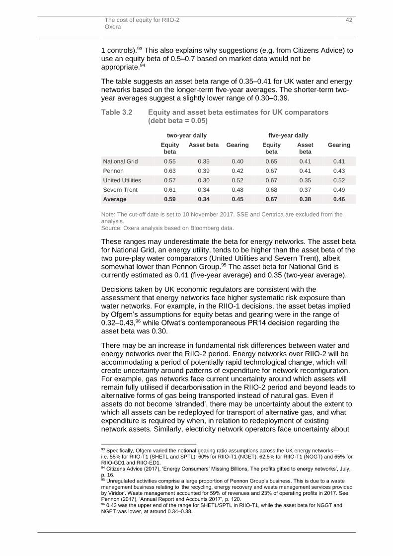
The cost of equity for RIIO-2 Oxera
42
1 controls).93 This also explains why suggestions (e.g. from Citizens Advice) to use an equity beta of 0.5–0.7 based on market data would not be appropriate.94
The table suggests an asset beta range of 0.35–0.41 for UK water and energy networks based on the longer-term five-year averages. The shorter-term two-year averages suggest a slightly lower range of 0.30–0.39.
Table 3.2 Equity and asset beta estimates for UK comparators (debt beta = 0.05)
two-year daily five-year daily
Equity beta
Asset beta Gearing Equity beta
Asset beta
Gearing
National Grid 0.55 0.35 0.40 0.65 0.41 0.41
Pennon 0.63 0.39 0.42 0.67 0.41 0.43
United Utilities 0.57 0.30 0.52 0.67 0.35 0.52
Severn Trent 0.61 0.34 0.48 0.68 0.37 0.49
Average 0.59 0.34 0.45 0.67 0.38 0.46
Note: The cut-off date is set to 10 November 2017. SSE and Centrica are excluded from the analysis. Source: Oxera analysis based on Bloomberg data.
These ranges may underestimate the beta for energy networks. The asset beta for National Grid, an energy utility, tends to be higher than the asset beta of the two pure-play water comparators (United Utilities and Severn Trent), albeit somewhat lower than Pennon Group.95 The asset beta for National Grid is currently estimated as 0.41 (five-year average) and 0.35 (two-year average).
Decisions taken by UK economic regulators are consistent with the assessment that energy networks face higher systematic risk exposure than water networks. For example, in the RIIO-1 decisions, the asset betas implied by Ofgem’s assumptions for equity betas and gearing were in the range of 0.32–0.43,96 while Ofwat’s contemporaneous PR14 decision regarding the asset beta was 0.30.
There may be an increase in fundamental risk differences between water and energy networks over the RIIO-2 period. Energy networks over RIIO-2 will be accommodating a period of potentially rapid technological change, which will create uncertainty around patterns of expenditure for network reconfiguration. For example, gas networks face current uncertainty around which assets will remain fully utilised if decarbonisation in the RIIO-2 period and beyond leads to alternative forms of gas being transported instead of natural gas. Even if assets do not become ‘stranded’, there may be uncertainty about the extent to which all assets can be redeployed for transport of alternative gas, and what expenditure is required by when, in relation to redeployment of existing network assets. Similarly, electricity network operators face uncertainty about
93 Specifically, Ofgem varied the notional gearing ratio assumptions across the UK energy networks—i.e. 55% for RIIO-T1 (SHETL and SPTL); 60% for RIIO-T1 (NGET); 62.5% for RIIO-T1 (NGGT) and 65% for RIIO-GD1 and RIIO-ED1. 94 Citizens Advice (2017), ‘Energy Consumers’ Missing Billions, The profits gifted to energy networks’, July, p. 16. 95 Unregulated activities comprise a large proportion of Pennon Group’s business. This is due to a waste management business relating to ‘the recycling, energy recovery and waste management services provided by Viridor’. Waste management accounted for 59% of revenues and 23% of operating profits in 2017. See Pennon (2017), ‘Annual Report and Accounts 2017’, p. 120. 96 0.43 was the upper end of the range for SHETL/SPTL in RIIO-T1, while the asset beta for NGGT and NGET was lower, at around 0.34–0.38.
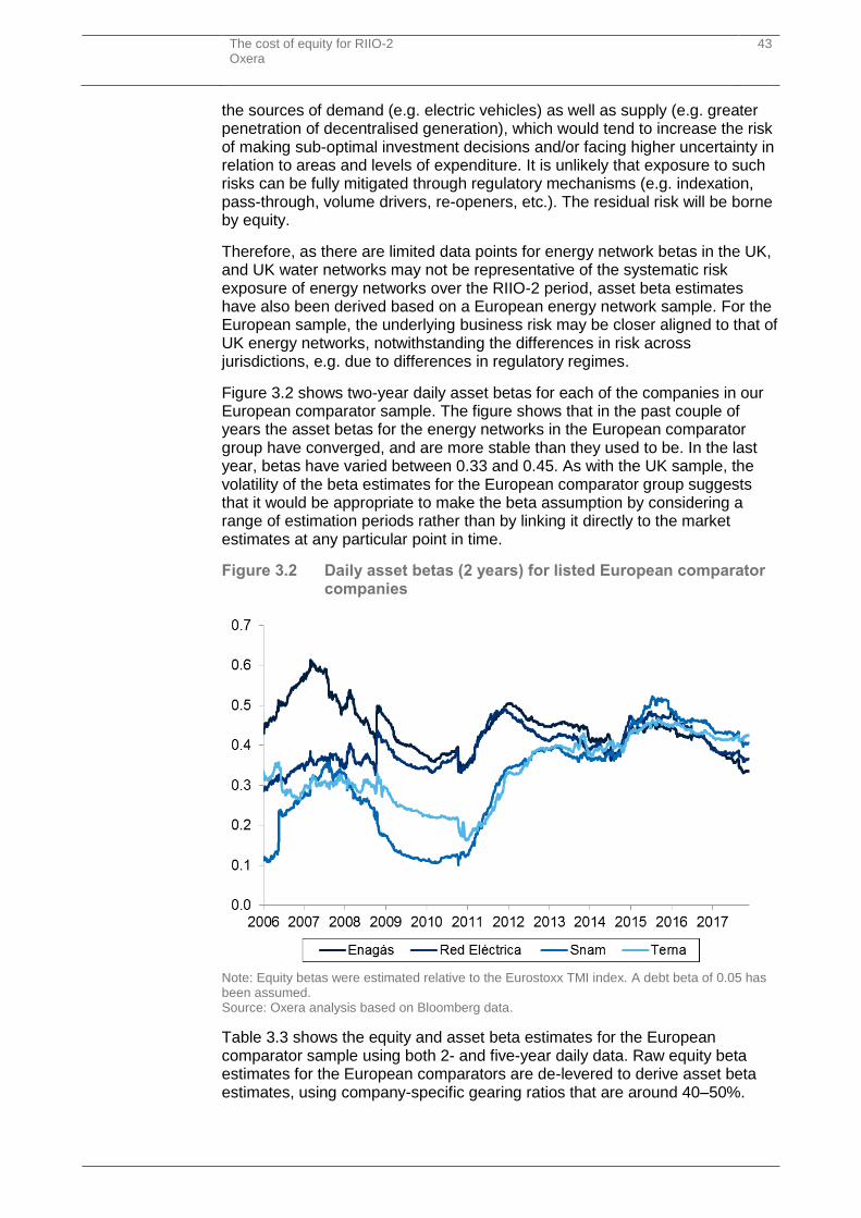
The cost of equity for RIIO-2 Oxera
43
the sources of demand (e.g. electric vehicles) as well as supply (e.g. greater penetration of decentralised generation), which would tend to increase the risk of making sub-optimal investment decisions and/or facing higher uncertainty in relation to areas and levels of expenditure. It is unlikely that exposure to such risks can be fully mitigated through regulatory mechanisms (e.g. indexation, pass-through, volume drivers, re-openers, etc.). The residual risk will be borne by equity.
Therefore, as there are limited data points for energy network betas in the UK, and UK water networks may not be representative of the systematic risk exposure of energy networks over the RIIO-2 period, asset beta estimates have also been derived based on a European energy network sample. For the European sample, the underlying business risk may be closer aligned to that of UK energy networks, notwithstanding the differences in risk across jurisdictions, e.g. due to differences in regulatory regimes.
Figure 3.2 shows two-year daily asset betas for each of the companies in our European comparator sample. The figure shows that in the past couple of years the asset betas for the energy networks in the European comparator group have converged, and are more stable than they used to be. In the last year, betas have varied between 0.33 and 0.45. As with the UK sample, the volatility of the beta estimates for the European comparator group suggests that it would be appropriate to make the beta assumption by considering a range of estimation periods rather than by linking it directly to the market estimates at any particular point in time.
Figure 3.2 Daily asset betas (2 years) for listed European comparator companies
Note: Equity betas were estimated relative to the Eurostoxx TMI index. A debt beta of 0.05 has been assumed. Source: Oxera analysis based on Bloomberg data.
Table 3.3 shows the equity and asset beta estimates for the European comparator sample using both 2- and five-year daily data. Raw equity beta estimates for the European comparators are de-levered to derive asset beta estimates, using company-specific gearing ratios that are around 40–50%.

The cost of equity for RIIO-2 Oxera
44
Table 3.3 Equity and asset beta estimates for European comparators (debt beta = 0.05)
two-year daily five-year daily
Equity beta
Asset beta Gearing Equity beta
Asset beta Gearing
Enagas 0.55 0.33 0.43 0.66 0.40 0.42
Red Eléctrica 0.54 0.36 0.36 0.66 0.41 0.41
Snam 0.69 0.40 0.45 0.80 0.45 0.47
Terna 0.75 0.42 0.47 0.77 0.42 0.48
Average 0.63 0.38 0.43 0.72 0.42 0.45
Note: The cut-off date is set to 10 November 2017. Source: Oxera analysis based on Bloomberg data.
Asset betas for the European sample lie in the range of 0.40–0.45 based on the longer-term five-year averages. The shorter-term two-year averages suggest a wider and lower range of 0.33–0.42. All of these companies derive almost all of their revenues from the regulated part of the business, and may therefore be considered pure-play energy networks.97 This points towards a higher asset beta for energy networks compared with the water companies that dominate the UK sample. Taking the evidence from the UK and European samples together suggests that a range of 0.38–0.42 is an appropriate assumption for the asset beta of UK energy networks.
3.5 Concluding remarks: risk and CAPM-based beta estimates
The empirical analysis presented in this section shows the following.
The UK sample of National Grid and three listed water companies produces a range of estimates for the asset beta (un-levered equity beta) of 0.35–0.41 based on the longer-term five-year averages. This assumes a debt beta of 0.05. The shorter-term two-year averages suggest a lower range of 0.30–0.39, which highlights the sensitivity of the estimates to the choice of measurement period. These ranges may underestimate the beta for energy networks. The asset beta for National Grid, an energy utility, tends to be higher than the asset beta of the two pure-play water comparators (United Utilities and Severn Trent), and is currently estimated as 0.41 (five-year average) and 0.35 (two-year average).
Notwithstanding differences in risk across jurisdictions, asset betas for a sample of four European energy networks (Enagas, Red Eléctrica, Snam, Terna) might be considered more representative of the asset risk of GB energy networks. Asset betas for this sample are in the range of 0.40–0.45 based on the longer-term five-year averages. As with the UK sample, this assumes a debt beta of 0.05. The shorter-term two-year averages suggest a lower range of 0.33–0.42. This points towards a higher asset beta for energy networks compared with the water companies that dominate the UK sample.
On balance, the evidence from the UK and European samples and the five- and two-year averages suggests an attenuated asset beta range of 0.38–0.42. This is consistent with energy networks having greater exposure to risk than water companies.
97 Source: Annual reports.

The cost of equity for RIIO-2 Oxera
45
The CAPM framework, while remaining the most widely used model for estimating the cost of equity, is based on assumptions, some of which may not always hold in practice. Some of the shortcomings are reviewed in Appendix 1.
Tests of the empirical performance of the CAPM have revealed many ‘anomalies’ that suggest that the accuracy of the standard CAPM in predicting the cost of equity decreases the further away the equity beta is from unity.98 One of the most relevant shortcomings is from empirical evidence in the USA, which suggests that stocks with a low beta (such as utility companies) consistently outperformed high-beta stocks over the period from January 1968 to December 2008. This is the ‘low beta anomaly’, which suggests that application of the CAPM tends to lead to an underestimate of the beta for stocks with relatively low betas, such as utilities. This runs counter to the CAPM prediction that there is a linear relationship between beta and returns. As the comparator companies used in this report have equity betas significantly lower than one when measured at market levels of gearing, adopting an asset beta estimate in the top half of the estimated asset beta range would provide some offset to this downward bias.
Furthermore, the literature on arbitrage pricing theory and multi-factor models suggests that there could be systematic risk factors that are not picked up in the CAPM market beta but are nevertheless priced by investors.99 The impact of the wider risk environment faced by energy networks can be accounted for when interpreting the outputs from the CAPM. In the context of UK energy networks, the extent and nature of the changes required to both electricity and gas distribution, and transmission, networks to facilitate energy decarbonisation and the necessary innovations in technologies required have created uncertainty over the future configuration of the energy system.
Consideration of the risks facing energy networks and the empirical shortcomings of the CAPM suggests selecting a beta point estimate in the top half of the attenuated range based on listed comparator companies. We recommend a range of 0.40–0.42 to inform the asset beta assumption for RIIO-2.
98 Asness, C., Moskowitz, T.J. and Pedersen, L.H. (2013), ‘Value and momentum everywhere’, The Journal of Finance, LXVIII: 3; Fama, E. and French, K. (2015), ‘Dissecting Anomalies with a Five-Factor Model’, The Review of Financial Studies, 29:1, 1 January 2016, pp. 69–103. 99 Chen, N., Roll, R. and Ross, S. (1986), ‘Economic Forces and the Stock Market’, The Journal of Business, 59:3, pp. 383–403; Ross, S. (1976), ‘The Arbitrage Theory of Capital Asset Pricing’, Journal of Economic Theory, 13, pp. 341–360.

The cost of equity for RIIO-2 Oxera
46
4 Required equity returns for RIIO-2
This section brings together the evidence from sections 2 and 3 on the estimates of the individual CAPM parameters in the context of RIIO-2 to produce a range for the real (RPI-deflated) cost of equity.
The section also examines where in the range the appropriate point estimates for the RIIO-2 controls are likely to lie. The following issues need to be considered:
the evidence suggests that the TMR is a more stable parameter than the ERP, and therefore that the top end of the TMR range is more likely to be correct than the bottom end;
consideration of the risks facing energy networks and the empirical shortcomings of the CAPM suggests selecting a beta point estimate in the top half of the beta range;
setting a point estimate above the middle of the cost of equity range reduces the risk of underinvestment;
regulated networks make investment decisions over very long horizons spanning multiple price control periods.
As evidence in relation to the first and second bullets has been presented in sections 2 and 3 respectively, this section discusses in turn the points raised in the third and fourth bullets. The section then concludes with the recommended range for the allowed cost of equity for RIIO-2.
4.1 Reducing the risk of underinvestment
In the absence of a sufficient allowed return on capital, investment may fall, resulting in an ‘underinvestment problem’. This problem is a form of regulatory failure with potentially significant adverse effects if it leads to a fall in the reliability and resilience of the network over time.
The underinvestment problem implies that there is both underinvestment, and that it becomes a problem. During price control periods, there will be flexibility to defer, or in some cases cancel, investment, although this is constrained to some degree by the incentives to deliver outputs or outcomes. Over the long term, the rational response to an allowed return lower than the cost of capital would be to develop business plans that minimise investment, with potential adverse consequences for reliability and innovation.
The issue has been expressed by Ofcom as follows:
If we were to set the regulated return too low relative to the true cost of capital the detriment from under-investment may exceed the detriment from setting too high a regulated return relative to the true cost of capital. A lower return than the true cost of capital will reduce BT’s incentives to invest and innovate in the regulated leased lines business and by restricting prices downstream, could reduce the incentives to invest by other infrastructure providers.100
Analysis undertaken by Oxera on behalf of the New Zealand Commerce Commission estimated the higher cost to consumers of setting the cost of capital too high, balanced against the lower cost from a reduced probability of
100 Ofcom (2016), ‘Business Connectivity Market Review’, 28 April, para. A30.238.

The cost of equity for RIIO-2 Oxera
47
underinvestment and consequent loss of network reliability.101 The report concluded that:
an estimate at the middle of the cost of capital range is likely to be too low as new investment adds no value to the company;
an estimate at the 90th percentile is likely to be too high in the context of electricity networks in New Zealand;
a shortfall of 0.5–1.0% (or more) in the cost of capital is likely to increase the risk of investment deferral;
a premium should be applied consistently over time across multiple price control periods as the expected whole-life return on investment is the relevant test for investors.
In the context of RIIO-2, an estimate at the middle of the cost of capital range is likely to be too low.
4.2 Providing a stable framework for long-term investment
Regulated networks make investment decisions over very long horizons spanning multiple price control periods, which would be supported by a regulatory regime that limits significant volatility in allowed returns from one price control period to the next. Limiting the change in the allowed return on equity for the RIIO-2 controls compared with the RIIO-1 controls would support long-term investment decisions.
4.3 Summary of the CAPM cost of equity estimates
Table 4.1 summarises the estimated range for the allowed cost of equity for UK energy networks in RIIO-2.
Table 4.1 Cost of equity for RIIO-2 (real, RPI-deflated)
Attenuated Recommended parameters Attenuated
Low Low High High
Real TMR (%) 5.50 6.00 6.50 6.50
Real RFR (%) -0.50 -0.50 0.00 0.00
ERP (%) 6.00 6.50 6.50 6.50
Asset beta 0.38 0.40 0.42 0.42
Gearing (%) 60 60 60 60
Equity beta 0.88 0.93 0.98 0.98
Debt beta 0.05 0.05 0.05 0.05
Real cost of equity (%) 4.75 5.51 6.34 6.34
Note: The estimates correspond to an RPI inflation assumption of 3.0%. Source: Oxera analysis.
A range of 5.51–6.34% is recommended to inform the assumption for the real (RPI-deflated) cost of equity in RIIO-2. This takes account of the following factors when moving from the attenuated range to a recommended range.
the attenuated range does not take full account of the weight of evidence in support of a relatively stable TMR;
101 Oxera (2014), ‘Input methodologies: review of the 75th percentile approach’, prepared for the New Zealand Commerce Commission, 23 June.

The cost of equity for RIIO-2 Oxera
48
the attenuated range relies on equity betas estimated for comparator companies that are significantly less than unity. Empirical tests find that the CAPM tends to under-predict returns for companies with equity betas lower than one;
the attenuated range may not fully reflect the wider risk environment faced by energy networks—in particular, the relatively high exposure of the sector to technological and political risks.
The next section considers alternative sources of evidence as points of comparison for the proposed range for the cost of equity.

The cost of equity for RIIO-2 Oxera
49
5 Alternative sources of evidence
This section provides alternative sources of evidence as points of comparison for the proposed range for the cost of equity from the previous section. The alternative sources of evidence are:
the asset risk premium (section 5.1);
the individual stock DDM (section 5.2);
regulatory precedent (section 5.3).
5.1 Asset risk premium
The asset risk premium is the additional compensation over the RFR that investors require to invest in a company as a whole. This is the premium for equity risk assuming zero gearing, and should be higher than the risk premium on debt given the lower priority of equity relative to debt in terms of claims on cash flows.
A risk premium on energy network assets would be expected to be greater than that on the investment-grade bonds that these companies issue. At the moment, the spreads for the A and BBB rated corporate bonds, used as a proxy for the bonds issued by the energy companies, are around 150bp.102
The CAPM parameters recommended in this report—an asset beta range of 0.40–0.42 and ERP of 6.5%—imply a range for the asset risk premium of 260–273bp. This is the premium for risk for an equity security with zero gearing. We would expect such a security to offer a higher risk premium than high-quality debt securities given the lower priority of equity relative to debt in the order of claims on cash flows and assets. The asset risk premium of 260–273bp compared with 150bp on bonds looks relatively modest.
5.2 Individual stock dividend discount model
A DDM, similar to that used to estimate the ERP and TMR, is applied to the UK-listed networks to check the cost of equity estimates implied by the CAPM. A one-stage DDM was used, with a long-term dividend growth forecast equal to the five-year nominal UK GDP growth rate.103 The long-term growth rate assumption is the same as used in the simple market DDM model presented in section 2. The results from this analysis are presented in Table 5.1.
Table 5.1 DDM cost of equity estimates (%)
November 2017 6-month average to November 2017
National Grid 8.9 8.6
Pennon 8.4 8.3
United Utilities 8.7 8.3
Severn Trent 7.7 7.6
Average 8.4 8.2
Source: Oxera analysis based on Bloomberg, Thomson Reuters Datastream, and IMF World Economic Outlook.
102 Based on the average spreads between yields on iBoxx £ A and BBB 10+ non-financial indices and yields on the UK government bonds with matching duration. This comparison is simplified and makes no adjustment for expected loss or debt beta. 103 Based on the IMF World Economic Outlook.

The cost of equity for RIIO-2 Oxera
50
The latest estimate of the cost of equity averaged across listed UK utilities under the DDM approach is 8.4% or 8.2% if a six-month average is considered. For National Grid the estimates are 8.9% and 8.6% respectively. This suggests a higher cost of equity for energy networks than water companies. Expressing the National Grid estimates in real terms using a 3% RPI inflation assumption provides a range of 5.6–5.9%.
As noted earlier, the cost of equity estimates under the DDM are very sensitive to the model inputs—in particular, the long-term growth rate assumption. These cost of equity estimates for single stocks, using a single-stage DDM are conservative, for two reasons:
the DDM analysis shown is based on market gearing (net debt / enterprise value) and the cost of equity estimates would need to be re-levered using the regulatory gearing assumption;
the implied real dividend growth rate used as an input to the DDM may be lower than company-specific growth. For example, it is lower than the real rate of growth observed for the RAV of National Grid (around 4% per annum).
The cost of equity range of 5.51–6.34% recommended in this report is therefore broadly consistent with a 5.6–5.9% cost of equity estimated by applying a DDM to National Grid Group, especially as the DDM for National Grid Group is likely to be an underestimate for the purposes of RIIO-2 as explained above.
5.3 Regulatory precedent
This section considers UK and international precedent on the allowed cost of equity and the allowed cost of capital. In particular, section 5.3.1 reviews the allowed cost of equity and cost of capital adopted in recent regulatory decisions in the UK across the economic regulated sectors. Section 5.3.2 then considers regulatory precedent for energy networks from Europe, covering Belgium, France, Germany, Ireland (including Northern Ireland), Italy, the Netherlands, and Portugal.
This UK and European regulatory precedent is complemented in section 5.3.3 by a review of the allowed return on equity for US investor-owned electric companies from base-rate filings.
In addition to providing a sense-check for the estimates from section 4, international regulatory precedent provides context for envisaging an international competition for capital. For example, return on equity benchmarks used by regulators in the USA and some countries in Europe are at higher levels than in the UK. This means that there is a risk that infrastructure capital may seek more attractive returns in other countries.
The evidence on international benchmarks also shows that countries such as Germany and the Netherlands have made relatively low cost of equity assumptions, although these regulators follow relatively mechanistic approaches to determining the parameters.104
104 For example, the Netherlands and Germany respectively use three- and ten-year averages for the RFR.
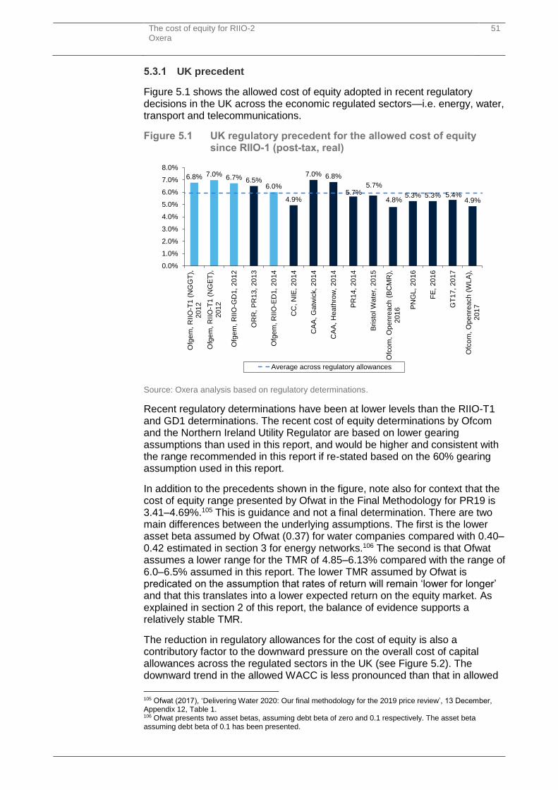
The cost of equity for RIIO-2 Oxera
51
5.3.1 UK precedent
Figure 5.1 shows the allowed cost of equity adopted in recent regulatory decisions in the UK across the economic regulated sectors—i.e. energy, water, transport and telecommunications.
Figure 5.1 UK regulatory precedent for the allowed cost of equity since RIIO-1 (post-tax, real)
Source: Oxera analysis based on regulatory determinations.
Recent regulatory determinations have been at lower levels than the RIIO-T1 and GD1 determinations. The recent cost of equity determinations by Ofcom and the Northern Ireland Utility Regulator are based on lower gearing assumptions than used in this report, and would be higher and consistent with the range recommended in this report if re-stated based on the 60% gearing assumption used in this report.
In addition to the precedents shown in the figure, note also for context that the cost of equity range presented by Ofwat in the Final Methodology for PR19 is 3.41–4.69%.105 This is guidance and not a final determination. There are two main differences between the underlying assumptions. The first is the lower asset beta assumed by Ofwat (0.37) for water companies compared with 0.40–0.42 estimated in section 3 for energy networks.106 The second is that Ofwat assumes a lower range for the TMR of 4.85–6.13% compared with the range of 6.0–6.5% assumed in this report. The lower TMR assumed by Ofwat is predicated on the assumption that rates of return will remain ‘lower for longer’ and that this translates into a lower expected return on the equity market. As explained in section 2 of this report, the balance of evidence supports a relatively stable TMR.
The reduction in regulatory allowances for the cost of equity is also a contributory factor to the downward pressure on the overall cost of capital allowances across the regulated sectors in the UK (see Figure 5.2). The downward trend in the allowed WACC is less pronounced than that in allowed
105 Ofwat (2017), ‘Delivering Water 2020: Our final methodology for the 2019 price review’, 13 December, Appendix 12, Table 1. 106 Ofwat presents two asset betas, assuming debt beta of zero and 0.1 respectively. The asset beta assuming debt beta of 0.1 has been presented.
6.8% 7.0% 6.7% 6.5%6.0%
4.9%
7.0% 6.8%
5.7%5.7%
4.8%5.3% 5.3% 5.4%
4.9%
0.0%
1.0%
2.0%
3.0%
4.0%
5.0%
6.0%
7.0%
8.0%
Ofg
em
, R
IIO
-T1 (
NG
GT
),201
2
Ofg
em
, R
IIO
-T1 (
NG
ET
),201
2
Ofg
em
, R
IIO
-GD
1, 201
2
OR
R,
PR
13, 201
3
Ofg
em
, R
IIO
-ED
1, 2
014
CC
, N
IE, 2
01
4
CA
A, G
atw
ick, 2
014
CA
A, H
eath
row
, 201
4
PR
14
, 2014
Bri
sto
l W
ate
r, 2
015
Ofc
om
, O
penre
ach
(B
CM
R),
201
6 PN
GL, 20
16
FE
, 2
016
GT
17
, 2017
Ofc
om
, O
penre
ach
(W
LA
),201
7
Average across regulatory allowances
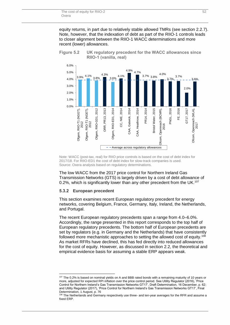
The cost of equity for RIIO-2 Oxera
52
equity returns, in part due to relatively stable allowed TMRs (see section 2.2.7). Note, however, that the indexation of debt as part of the RIIO-1 controls leads to closer alignment between the RIIO-1 WACC determinations and more recent (lower) allowances.
Figure 5.2 UK regulatory precedent for the WACC allowances since RIIO-1 (vanilla, real)
Note: WACC (post-tax, real) for RIIO price controls is based on the cost of debt index for 2017/18. For RIIO-ED1 the cost of debt index for slow-track companies is used. Source: Oxera analysis based on regulatory determinations.
The low WACC from the 2017 price control for Northern Ireland Gas Transmission Networks (GTS) is largely driven by a cost of debt allowance of 0.2%, which is significantly lower than any other precedent from the UK.107
5.3.2 European precedent
This section examines recent European regulatory precedent for energy networks, covering Belgium, France, Germany, Italy, Ireland, the Netherlands, and Portugal.
The recent European regulatory precedents span a range from 4.0–6.0%. Accordingly, the range presented in this report corresponds to the top half of European regulatory precedents. The bottom half of European precedents are set by regulators (e.g. in Germany and the Netherlands) that have consistently followed more mechanistic approaches to setting the allowed cost of equity.108 As market RFRs have declined, this has fed directly into reduced allowances for the cost of equity. However, as discussed in section 2.2, the theoretical and empirical evidence basis for assuming a stable ERP appears weak.
107 The 0.2% is based on nominal yields on A and BBB rated bonds with a remaining maturity of 10 years or more, adjusted for expected RPI inflation over the price control period. See Utility Regulator (2016), ‘Price Control for Northern Ireland’s Gas Transmission Networks GT17’, Draft Determination, 16 December, p. 62; and Utility Regulator (2017), ‘Price Control for Northern Ireland’s Gas Transmission Networks GT17’, Final Determination, 1 August, p. 76 108 The Netherlands and Germany respectively use three- and ten-year averages for the RFR and assume a fixed ERP.
3.9% 4.1%3.8%
4.3%
3.6%4.1%
4.9%4.7%
3.7% 3.8%4.0%
3.7%3.7%
2.0%
3.6%
0.0%
1.0%
2.0%
3.0%
4.0%
5.0%
6.0%
Ofg
em
, R
IIO
-T1 (
NG
GT
),201
2
Ofg
em
, R
IIO
-T1 (
NG
ET
),201
2
Ofg
em
, R
IIO
-GD
1, 201
2
OR
R, P
R13, 201
3
Ofg
em
, R
IIO
-ED
1, 2
014
CC
, N
IE, 2
01
4
CA
A, G
atw
ick, 2
014
CA
A, H
eath
row
, 201
4
PR
14
, 2014
Bri
sto
l W
ate
r, 2
015
Ofc
om
, O
penre
ach
(B
CM
R),
201
6 PN
GL, 20
16
FE
, 2
016
GT
17
, 2017
Ofc
om
, O
penre
ach
(W
LA
),201
7
Average across regulatory allowances

The cost of equity for RIIO-2 Oxera
53
Figure 5.3 European regulatory precedent for the cost of equity (post-tax, real)
Note: Portugal (P) and Belgium (B): 2% inflation assumption used to derive the real RFR. Portugal (P): in deriving the cost of equity, country risk premium is added to the ERP rather than the RFR. Source: Oxera analysis based on regulatory determinations.
Figure 5.4 shows recent European regulatory determinations on the allowed WACC. The allowed WACC for energy networks in Europe since 2014 has been lower than in the RIIO-1 price controls, with a particularly low level of allowed returns in the Netherlands and Belgium.
Figure 5.4 European regulatory precedent for the WACC (vanilla, real)
Note: IRL 2015–DSO: the baseline pre-tax WACC of 4.74% is increased to 4.95% to account for an ‘aiming up’ allowance (not presented in the chart above). Portugal (P) and Belgium (B): 2% inflation assumption used to derive the real RFR. Source: Oxera analysis based on regulatory determinations.
0.0%
1.0%
2.0%
3.0%
4.0%
5.0%
6.0%
7.0%
P 2
014 –
ET
P 2
014 –
ED
IT 2
015 –
ET
IT 2
015 –
ED
IRL 2
015 –
DS
O
DE
201
6 –
Energ
y
NL 2
016 –
Energ
y
FR
2016 –
ET
FR
2016 –
GT
P 2
016 –
GT
P 2
016 –
GD
B 2
016 –
VR
EG
(D
istr
)
IRL 2
017 –
GD
B 2
017 –
CW
aP
E (
Dis
tr)
Cost of equity real, post-tax
0.0%
0.5%
1.0%
1.5%
2.0%
2.5%
3.0%
3.5%
4.0%
4.5%
5.0%
P 2
014 –
ET
P 2
014 –
ED
IT 2
015 –
ET
IT 2
015 –
ED
IRL 2
015 –
DS
O
NL 2
016 –
Energ
y
FR
2016 –
ET
FR
2016 –
GT
P 2
016 –
GT
P 2
016 –
GD
B 2
016 –
VR
EG
(D
istr
)
IRL 2
017 –
GD
B 2
017 –
CW
aP
E (
Dis
tr)
WACC vanilla, real
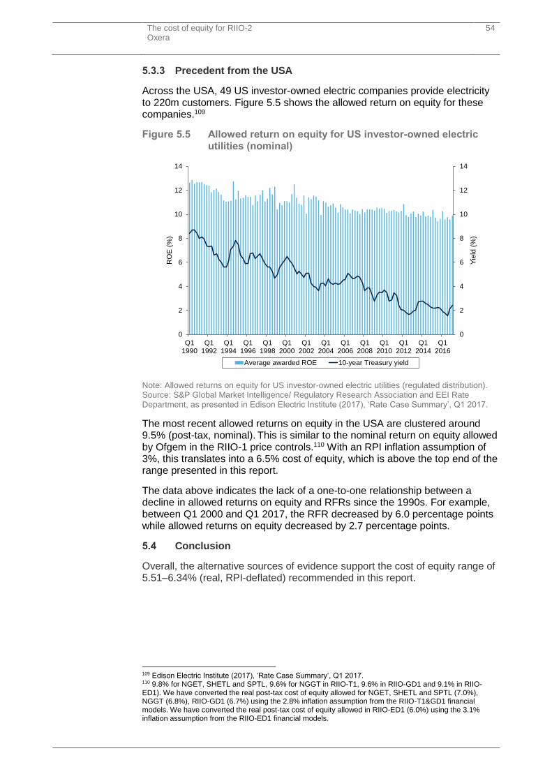
The cost of equity for RIIO-2 Oxera
54
5.3.3 Precedent from the USA
Across the USA, 49 US investor-owned electric companies provide electricity to 220m customers. Figure 5.5 shows the allowed return on equity for these companies.109
Figure 5.5 Allowed return on equity for US investor-owned electric utilities (nominal)
Note: Allowed returns on equity for US investor-owned electric utilities (regulated distribution). Source: S&P Global Market Intelligence/ Regulatory Research Association and EEI Rate Department, as presented in Edison Electric Institute (2017), ‘Rate Case Summary’, Q1 2017.
The most recent allowed returns on equity in the USA are clustered around 9.5% (post-tax, nominal). This is similar to the nominal return on equity allowed by Ofgem in the RIIO-1 price controls.110 With an RPI inflation assumption of 3%, this translates into a 6.5% cost of equity, which is above the top end of the range presented in this report.
The data above indicates the lack of a one-to-one relationship between a decline in allowed returns on equity and RFRs since the 1990s. For example, between Q1 2000 and Q1 2017, the RFR decreased by 6.0 percentage points while allowed returns on equity decreased by 2.7 percentage points.
5.4 Conclusion
Overall, the alternative sources of evidence support the cost of equity range of 5.51–6.34% (real, RPI-deflated) recommended in this report.
109 Edison Electric Institute (2017), ‘Rate Case Summary’, Q1 2017. 110 9.8% for NGET, SHETL and SPTL, 9.6% for NGGT in RIIO-T1, 9.6% in RIIO-GD1 and 9.1% in RIIO-ED1). We have converted the real post-tax cost of equity allowed for NGET, SHETL and SPTL (7.0%), NGGT (6.8%), RIIO-GD1 (6.7%) using the 2.8% inflation assumption from the RIIO-T1&GD1 financial models. We have converted the real post-tax cost of equity allowed in RIIO-ED1 (6.0%) using the 3.1% inflation assumption from the RIIO-ED1 financial models.
0
2
4
6
8
10
12
14
0
2
4
6
8
10
12
14
Q11990
Q11992
Q11994
Q11996
Q11998
Q12000
Q12002
Q12004
Q12006
Q12008
Q12010
Q12012
Q12014
Q12016
Yie
ld (
%)
RO
E (
%)
Average awarded ROE 10-year Treasury yield
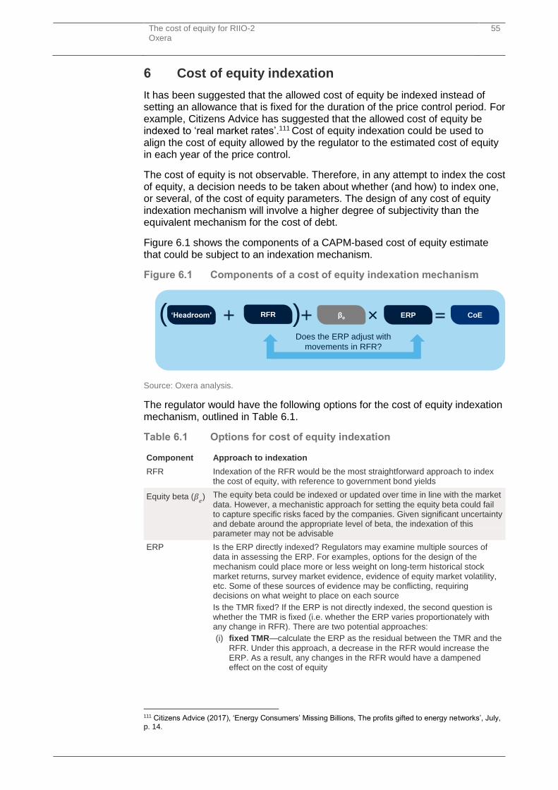
The cost of equity for RIIO-2 Oxera
55
6 Cost of equity indexation
It has been suggested that the allowed cost of equity be indexed instead of setting an allowance that is fixed for the duration of the price control period. For example, Citizens Advice has suggested that the allowed cost of equity be indexed to ‘real market rates’.111 Cost of equity indexation could be used to align the cost of equity allowed by the regulator to the estimated cost of equity in each year of the price control.
The cost of equity is not observable. Therefore, in any attempt to index the cost of equity, a decision needs to be taken about whether (and how) to index one, or several, of the cost of equity parameters. The design of any cost of equity indexation mechanism will involve a higher degree of subjectivity than the equivalent mechanism for the cost of debt.
Figure 6.1 shows the components of a CAPM-based cost of equity estimate that could be subject to an indexation mechanism.
Figure 6.1 Components of a cost of equity indexation mechanism
Source: Oxera analysis.
The regulator would have the following options for the cost of equity indexation mechanism, outlined in Table 6.1.
Table 6.1 Options for cost of equity indexation
Component Approach to indexation
RFR Indexation of the RFR would be the most straightforward approach to index the cost of equity, with reference to government bond yields
Equity beta (𝛽𝑒) The equity beta could be indexed or updated over time in line with the market
data. However, a mechanistic approach for setting the equity beta could fail to capture specific risks faced by the companies. Given significant uncertainty and debate around the appropriate level of beta, the indexation of this parameter may not be advisable
ERP Is the ERP directly indexed? Regulators may examine multiple sources of data in assessing the ERP. For examples, options for the design of the mechanism could place more or less weight on long-term historical stock market returns, survey market evidence, evidence of equity market volatility, etc. Some of these sources of evidence may be conflicting, requiring decisions on what weight to place on each source
Is the TMR fixed? If the ERP is not directly indexed, the second question is whether the TMR is fixed (i.e. whether the ERP varies proportionately with any change in RFR). There are two potential approaches:
(i) fixed TMR—calculate the ERP as the residual between the TMR and the
RFR. Under this approach, a decrease in the RFR would increase the ERP. As a result, any changes in the RFR would have a dampened effect on the cost of equity
111 Citizens Advice (2017), ‘Energy Consumers’ Missing Billions, The profits gifted to energy networks’, July, p. 14.
RFR βe ERP CoE‘Headroom’( )Does the ERP adjust with
movements in RFR?
The cost of equity for RIIO-2 Oxera
56
Component Approach to indexation
(ii) fixed ERP—set the ERP independently of the RFR. Under this
approach, a change in RFR would have a one-to-one effect on the cost of equity
6.1 Indexation of the market parameters
Indexation of the RFR would be the most straightforward approach to index the cost of equity. Key questions in specifying an RFR index for a cost of equity indexation mechanism are the choice of the index and the extent to which spot rates are translated into an RFR allowance. As discussed in section 2, the approach to the RFR cannot be considered in isolation from the ERP and the TMR.
6.1.1 Which index to use?
Data on the RFR is easily available. However, the regulator would have to choose the appropriate maturity of the RFR index—e.g. whether to use yields on 5-, 10- or 20-year index-linked gilts (ILGs). The long-term investment horizon of equity investment in the energy sector suggests that longer-term ILGs should be given more weight in an RFR index.112
6.1.2 How should changes in spot rates be translated into the RFR allowance?
Indexation of the cost of equity would lead to movements in the equity allowance in line with short-term market movements. However, this may lead to greater volatility in network charges. If promoting the stability of network charges is important, the regulator could use:
a trailing average (similar to the cost of debt mechanism)—a longer-term average would provide stability in the RFR allowance. However, such an approach may lead to underinvestment in the industry when a rapid increase in spot interest rates is not matched by an appropriate increase in the RFR allowance;
a dampening factor—the regulator could pass on a fraction of the changes in spot rates to the RFR allowance. This would ensure that the RFR allowance is updated in line with current market evidence, while providing some protection against short-term interest rate volatility. For example, if a dampening factor of 0.5 is used, a 100bp increase in the spot rates would translate into a 50bp increase in the RFR allowance.
6.1.3 Should the RFR be set above spot rates?
In recent regulatory precedent, allowed RFRs have been higher than spot rates to allow for market uncertainty. If the RFR is indexed to the market data, one consideration would be to decide how much residual uncertainty remains and how much headroom above market rates should be retained.
6.1.4 Fixed TMR or fixed ERP?
The choice between the two approaches of fixed TMR or fixed ERP is related to the discussion in section 2. Given that the balance of evidence in section 2 suggests the stability of the TMR, it would be relevant to jointly determine movements in the RFR and ERP, such that a movement (up or down) in the
112 For example, Ofgem’s five-year asset life assumption for new assets demonstrates that investors in energy assets face a long period to recoup the invested capital.
The cost of equity for RIIO-2 Oxera
57
RFR is largely offset by movements in the ERP.113 This would limit volatility in allowed returns within the price control period, and between periods.
6.2 Conclusion
Cost of equity indexation could be used to align the cost of equity allowed by the regulator to the estimated cost of equity in each year of the price control, and thereby minimise the risk of windfall gains and losses during the price control period.
Unlike the cost of debt, the cost of equity is not observable. Therefore, in any attempt to index the cost of equity, a decision needs to be taken about whether (and how) to index one, or several, of the cost of equity parameters. The design of any cost of equity indexation mechanism will involve a higher degree of subjectivity than the equivalent mechanism for the cost of debt.
The following principles for indexing the cost of equity emerge from the evidence examined in this report.
there is a negative correlation between the ERP and the RFR, which implies that indexation of only the RFR would create large errors;
the TMR is relatively stable over time, which implies that the TMR generated by the indexation mechanism should be relatively stable over time;
equity beta estimates are more volatile over time than would be expected given the relatively stable risk characteristics of the businesses. This implies that the beta parameters of the indexation mechanism should be more stable than the market estimates or should be fixed.
Overall, a move to cost of equity indexation would represent a considerable change in methodology. Such a change in methodology would need to fully take into account the principles above, be appropriately signalled, and be introduced with appropriate transitional arrangements such that it does not undermine investor confidence.
113 Depending on the level of the allowed equity beta. (An equity beta of unity would imply a one-for-one offset of movements in the RF, by movements in the ERP.)
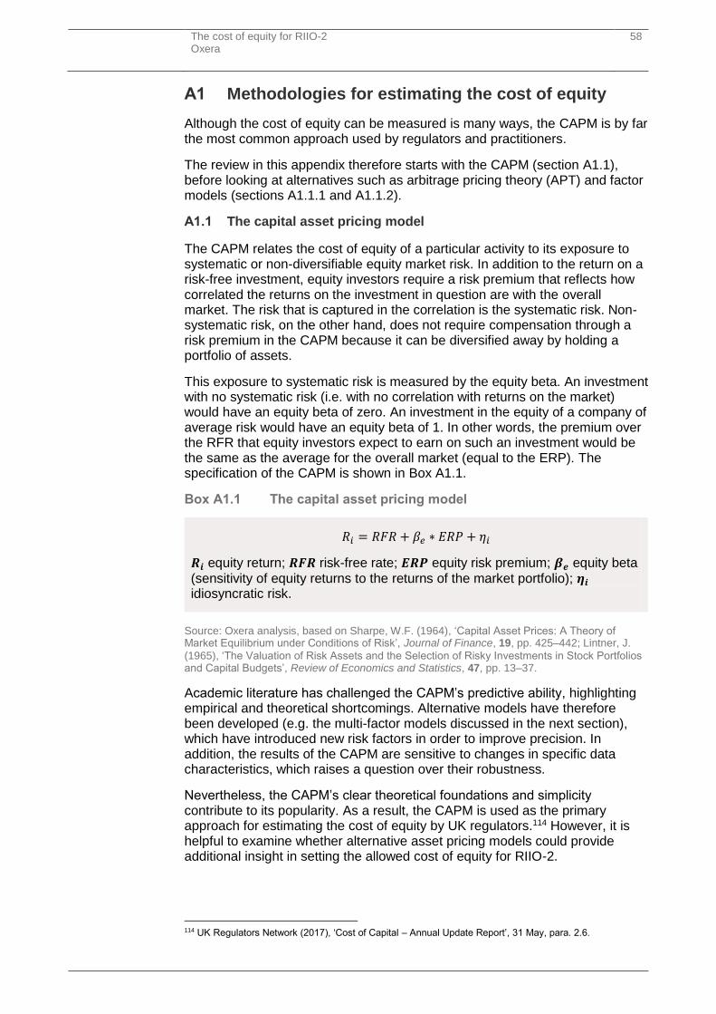
The cost of equity for RIIO-2 Oxera
58
A1 Methodologies for estimating the cost of equity
Although the cost of equity can be measured is many ways, the CAPM is by far the most common approach used by regulators and practitioners.
The review in this appendix therefore starts with the CAPM (section A1.1), before looking at alternatives such as arbitrage pricing theory (APT) and factor models (sections A1.1.1 and A1.1.2).
A1.1 The capital asset pricing model
The CAPM relates the cost of equity of a particular activity to its exposure to systematic or non-diversifiable equity market risk. In addition to the return on a risk-free investment, equity investors require a risk premium that reflects how correlated the returns on the investment in question are with the overall market. The risk that is captured in the correlation is the systematic risk. Non-systematic risk, on the other hand, does not require compensation through a risk premium in the CAPM because it can be diversified away by holding a portfolio of assets.
This exposure to systematic risk is measured by the equity beta. An investment with no systematic risk (i.e. with no correlation with returns on the market) would have an equity beta of zero. An investment in the equity of a company of average risk would have an equity beta of 1. In other words, the premium over the RFR that equity investors expect to earn on such an investment would be the same as the average for the overall market (equal to the ERP). The specification of the CAPM is shown in Box A1.1.
Box A1.1 The capital asset pricing model
𝑅𝑖 = 𝑅𝐹𝑅 + 𝛽𝑒 ∗ 𝐸𝑅𝑃 + 𝜂𝑖
𝑹𝒊 equity return; 𝑹𝑭𝑹 risk-free rate; 𝑬𝑹𝑷 equity risk premium; 𝜷𝒆 equity beta
(sensitivity of equity returns to the returns of the market portfolio); 𝜼𝒊 idiosyncratic risk.
Source: Oxera analysis, based on Sharpe, W.F. (1964), ‘Capital Asset Prices: A Theory of Market Equilibrium under Conditions of Risk’, Journal of Finance, 19, pp. 425–442; Lintner, J.
(1965), ‘The Valuation of Risk Assets and the Selection of Risky Investments in Stock Portfolios and Capital Budgets’, Review of Economics and Statistics, 47, pp. 13–37.
Academic literature has challenged the CAPM’s predictive ability, highlighting empirical and theoretical shortcomings. Alternative models have therefore been developed (e.g. the multi-factor models discussed in the next section), which have introduced new risk factors in order to improve precision. In addition, the results of the CAPM are sensitive to changes in specific data characteristics, which raises a question over their robustness.
Nevertheless, the CAPM’s clear theoretical foundations and simplicity contribute to its popularity. As a result, the CAPM is used as the primary approach for estimating the cost of equity by UK regulators.114 However, it is helpful to examine whether alternative asset pricing models could provide additional insight in setting the allowed cost of equity for RIIO-2.
114 UK Regulators Network (2017), ‘Cost of Capital – Annual Update Report’, 31 May, para. 2.6.

The cost of equity for RIIO-2 Oxera
59
A1.1.1 Arbitrage pricing theory
Finance theory predicts that systematic and non-diversifiable sources of risk will be priced in, and that investors will require higher returns for taking on exposure to such risks.115
APT, a multifactor model developed by Ross (1976), is based on the assumption that there should be no arbitrage opportunities in an economy.116 It looks at expected stock returns based on risk factors such as macroeconomic variables. Theoretically, APT could capture every single factor that explains stock returns.
While the CAPM considers only the correlation of returns with equity markets as a proxy for exposure to systematic risk, the model will not capture any additional sources of systematic risk that may affect required returns; these additional sources could be accounted for in APT.
In general, APT could be described by the pricing model in Box A1.2 .
Box A1.2 Arbitrage pricing theory
𝑅𝑖 = 𝑅𝐹𝑅 + 𝛽𝑖1 ∗ 𝐾1 + 𝛽𝑖2 ∗ 𝐾2 + ⋯ + 𝛽𝑖𝑘 ∗ 𝐾𝑘 + 𝜂𝑖
𝑹𝒊 equity return; 𝑹𝑭𝑹 risk-free rate; 𝑲𝒊𝒌 risk factor; 𝜷𝒊𝒌 sensitivity of equity returns to the risk factor K; 𝜼𝒊 idiosyncratic risk or residual term that is independent across securities.
APT could include any number of risk factors that could explain the equity returns. In theory, if there are no arbitrage opportunities, the equity return of any asset could be explained by K risk factors (i.e. there is no idiosyncratic risk). In practice, however, idiosyncratic risk would exist. Nevertheless, the linear relationship between the equity return and the risk factors may hold approximately—APT is better at explaining the equity returns as the idiosyncratic risk becomes smaller.
Source: Oxera analysis, based on Ross (1976), op. cit.; and Wright, Mason, and Miles (2003), op. cit., pp. 65–67.
The general formulation of the APT model does not help to identify an exhaustive list of relevant risk factors. In theory, any non-diversifiable risk factor could be added into the model. Therefore, the APT model supports a broader view of risk exposures than implied by the CAPM. However, the precise formulation and effect of these risk exposures on equity returns is not clear and should be tested empirically.
A1.1.2 Factor models
Fama and French (1993) proposed to add two factors in addition to the overall market factor captured by the CAPM: size factor and value factor. The size factor captures the additional return associated with companies that have small market capitalisation. The value factor captures the additional return associated with companies that have high book-to-market ratios. The specification of the three-factor model is outlined Box A1.3 below.
115 Chen, N., Roll, R. and Ross, S. (1986), ‘Economic Forces and the Stock Market’, The Journal of Business, 59:3, pp. 383–403. 116 Ross, S. (1976), ‘The Arbitrage Theory of Capital Asset Pricing’, Journal of Economic Theory, 13, pp. 341–360.
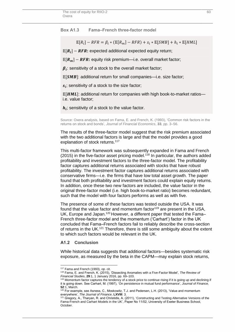
The cost of equity for RIIO-2 Oxera
60
Box A1.3 Fama–French three-factor model
𝔼[𝑅𝑖] − 𝑅𝐹𝑅 = 𝛽𝑖 ∗ (𝔼[𝑅𝑚] − 𝑅𝐹𝑅) + 𝑠𝑖 ∗ 𝔼[𝑆𝑀𝐵] + ℎ𝑖 ∗ 𝔼[𝐻𝑀𝐿]
𝔼[𝑹𝒊] − 𝑹𝑭𝑹: expected additional expected equity return;
𝔼[𝑹𝒎] − 𝑹𝑭𝑹: equity risk premium—i.e. overall market factor;
𝜷𝒊: sensitivity of a stock to the overall market factor;
𝔼[𝑺𝑴𝑩]: additional return for small companies—i.e. size factor;
𝒔𝒊; sensitivity of a stock to the size factor;
𝔼[𝑯𝑴𝑳]: additional return for companies with high book-to-market ratios—i.e. value factor;
𝒉𝒊; sensitivity of a stock to the value factor.
Source: Oxera analysis, based on Fama, E. and French, K. (1993), ‘Common risk factors in the returns on stock and bonds’, Journal of Financial Economics, 33, pp. 3–56.
The results of the three-factor model suggest that the risk premium associated with the two additional factors is large and that the model provides a good explanation of stock returns.117
This multi-factor framework was subsequently expanded in Fama and French (2015) in the five-factor asset pricing model.118 In particular, the authors added profitability and investment factors to the three-factor model. The profitability factor captures additional returns associated with stocks that have robust profitability. The investment factor captures additional returns associated with conservative firms—i.e. the firms that have low total asset growth. The paper found that both profitability and investment factors could explain equity returns. In addition, once these two new factors are included, the value factor in the original three-factor model (i.e. high book-to-market ratio) becomes redundant, such that the model with four factors performs as well as with five.
The presence of some of these factors was tested outside the USA. It was found that the value factor and momentum factor119 are present in the USA, UK, Europe and Japan.120 However, a different paper that tested the Fama–French three-factor model and the momentum (‘Carhart’) factor in the UK concluded that Fama–French factors fail to reliably describe the cross-section of returns in the UK.121 Therefore, there is still some ambiguity about the extent to which such factors would be relevant in the UK.
A1.2 Conclusion
While historical data suggests that additional factors—besides systematic risk exposure, as measured by the beta in the CAPM—may explain stock returns,
117 Fama and French (1993), op. cit. 118 Fama, E. and French, K. (2015), ‘Dissecting Anomalies with a Five-Factor Model’, The Review of Financial Studies, 29:1, 1 January 2016, pp. 69–103. 119 Momentum factor captures the tendency of a stock price to continue rising if it is going up and declining if it is going down. See Carhart, M. (1997), ‘On persistence in mutual fund performance’, Journal of Finance, 52:1, March. 120 For example, see Asness, C., Moskowitz, T.J. and Pedersen, L.H. (2013), ‘Value and momentum everywhere’, The Journal of Finance, LXVIII: 3. 121 Gregory, A., Tharyan, R. and Christidis, A. (2011), ‘Constructing and Testing Alternative Versions of the Fama-French and Carhart Models in the UK’, Paper No 11/02, University of Exeter Business School, October.

The cost of equity for RIIO-2 Oxera
61
which factors are relevant, and the extent to which these factors would persist in the future, as well as the size of the premium associated with these factors is not certain. Additionally, the exposure (or factor loadings) of ENA member companies to additional factors, such as the Fama–French factors, would be difficult to estimate.
As a result, the CAPM has been used in this report as the primary model for estimating the cost of equity for energy networks for RIIO-2. The impact of the wider risk environment faced by energy networks can be accounted for when interpreting the outputs from the CAPM.

www.oxera.com