THE CONTRIBUTION OF INFORMATION COMMUNICATION …studentsrepo.um.edu.my/4630/1/Final_Vesrion_of_Ph.D_Thesis.18_March_2014.pdfthe contribution of information communication technology

THE CONTRIBUTION OF INFORMATION COMMUNICATION

TECHNOLOGY (ICT) TO TOTAL FACTOR PRODUCTIVITY

(TFP) AND ECONOMIC GROWTH:

EVIDENCE FROM ASIA-PACIFIC AND EU COUNTRIES

FARZANEH KHALILI

FACULTY OF ECONOMICS AND ADMINISTRATION

UNIVERSITY OF MALAYA

KUALA LUMPUR

2014

I

THE CONTRIBUTION OF INFORMATION COMMUNICATION

TECHNOLOGY (ICT) TO TOTAL FACTOR PRODUCTIVITY

(TFP) AND ECONOMIC GROWTH:

EVIDENCE FROM ASIA-PACIFIC AND EU COUNTRIES

FARZANEH KHALILI

THESIS SUBMITTED IN FULFILMENT

OF THE REQUIREMENT

FOR THE DEGREE OF DOCTOR OF PHILOSOPHY

FACULTY OF ECONOMICS AND ADMINISTRATION

UNIVERSITY OF MALAYA

KUALA LUMPUR

2014

II

UNIVERSITY OF MALAYA ORIGINAL LITERARY WORK DECLARATION

Name of Candidate: Farzaneh Khalili

Matric No: EHA090018

Name of Degree: Doctor of Philosophy

Title of Research Paper: The Contribution of Information Communication Technology

(ICT) to Total Factor Productivity (TFP) and Economic Growth: Evidence from Asia-

Pacific and EU Countries

Field of Study: Industrial Economics

I do solemnly and sincerely declare that:

(1) I am the sole author / writer of this Work;

(2) The Work is original;

(3) Any use of any work in which copyright exists was done by way of fair dealing and

for permitted purposes and any excerpt or extract form, or reference to or reproduction

of any copyright work has been disclosed expressly and sufficiently and the title of the

Work and its authorship have been acknowledged in this Work;

(4) I do not have any actual knowledge nor do I ought reasonably to know that the

making of this work constitutes an infringement of any copyright work;

(5) I hereby assign all and every rights in the copyright to this Work to the University

of Malaya (“UM”), who henceforth shall be owner of the copyright in this Work and

that any reproduction or use in any form or by any means whatsoever is prohibited

without written consent of UM having been first had and obtained;

(6) I am fully aware that if in the course of making this Work I have infringed any

copyright whether intentionally or otherwise, I may be subject to legal action or any

other action as may be determined by UM.

Candidate’s Signature Date

Subscribed and solemnly declared before,

Witness’s Signature

Name:

Designation:

III

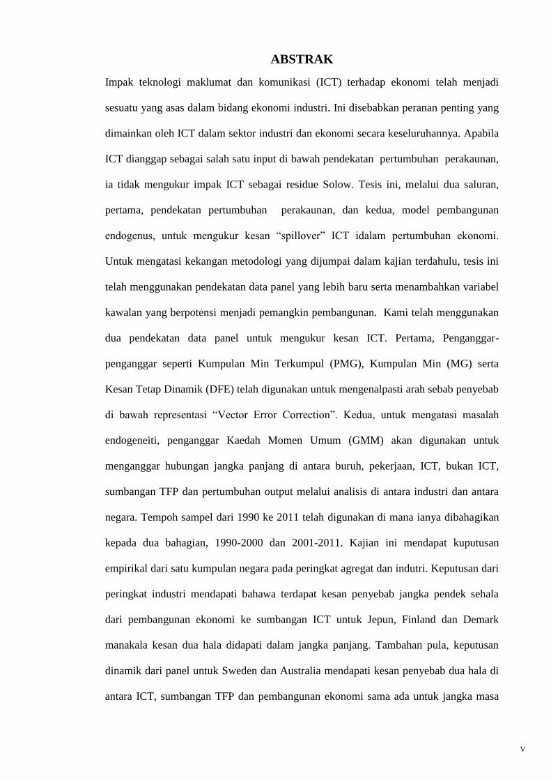
ABSTRACT

The impact of information and communications technology (ICT) on the economy has

become a fundamental part of industrial economics. This is due to the key role played

by ICT in the industrial sector and economy as a whole. When ICT is considered as just

an input under the growth accounting approach, it fails to capture the impact of ICT as a

Solow residual. This thesis, through the use of two channels, firstly, the growth

accounting approach, and, secondly, the endogenous growth model, fully captures the

spillover effects of ICT on economic growth. To overcome the methodological

limitation found in previous studies, this thesis has adopted a relatively new panel data

techniques and added new controlling variables that are expected to have potential as

additional growth drivers. We have used two different panel data approaches to estimate

the ICT effects. Firstly, Pooled Mean Group (PMG), Mean Group (MG) and Dynamic

Fixed Effect (DFE) estimators are applied to identify the direction of causality under

vector error correction representation. Secondly, to deal with the endogeneity problem,

Generalised Methods of Moments (GMM) estimators are employed to estimate the long

run association among labour employment, ICT, non-ICT, TFP contribution and output

growth through cross-industry and cross-country analyses. The sample period covers

from 1990 to 2011 of which is further divided into two sub-periods, 1990 to 2000 and

2001 to 2011 respectively. This study obtains empirical results from a group of

countries at the aggregate and industrial levels. The industrial level findings reveal that

there is a unidirectional short run causal relationship running from economic growth to

ICT contribution for Japan, Finland and Denmark but that relationship is bidirectional in

the long run. Furthermore, the dynamic panel results for Sweden and Australia show

bidirectional causality among ICT, TFP contribution and economic growth both in the

long run and short run. ICT has no significant effect on TFP growth in Japan and

Finland, whereas a negative relationship between ICT and TFP may reveal a

IV

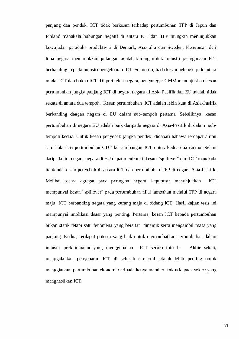
productivity paradox in Denmark, Australia and Sweden. The outcomes in five

countries show that returns were smaller in ICT-using than ICT-producing industries

and that no significant complementary impacts exist between ICT and non-ICT capital.

At the country level, GMM estimates indicate that the long run growth impact of ICT in

the Asia-Pacific and EU countries is not uniform between two sub-periods. The growth

impact of ICT was stronger in Asia-Pacific countries during the first sub-period as

opposed to the EU. In contrast, EU led Asia-Pacific countries in the second sub-period.

For short run causality, it is found that there is unidirectional flow from GDP growth to

ICT contribution for both regions. Moreover, the EU countries benefit from the

spillover effects of ICT whereas there is no causal relationship between ICT and TFP

growth in Asia-Pacific countries. Aggregating at the country level, the result reveals

that ICT has a higher positive spillover effect on value added growth through TFP in

ICT developed countries as compared to ICT less developed countries. The thesis

concludes with a few policy implications. First, the effect of ICT on growth is not static

but a long and dynamic process. Second, there is robust potential to exploit growth

profits in service industries that make intensive use of ICT. Finally, advocating ICT

diffusion within the economy is much more growth enhancing than just concentrating

on the ICT-producing sectors.

V

ABSTRAK

Impak teknologi maklumat dan komunikasi (ICT) terhadap ekonomi telah menjadi

sesuatu yang asas dalam bidang ekonomi industri. Ini disebabkan peranan penting yang

dimainkan oleh ICT dalam sektor industri dan ekonomi secara keseluruhannya. Apabila

ICT dianggap sebagai salah satu input di bawah pendekatan pertumbuhan perakaunan,

ia tidak mengukur impak ICT sebagai residue Solow. Tesis ini, melalui dua saluran,

pertama, pendekatan pertumbuhan perakaunan, dan kedua, model pembangunan

endogenus, untuk mengukur kesan “spillover” ICT idalam pertumbuhan ekonomi.

Untuk mengatasi kekangan metodologi yang dijumpai dalam kajian terdahulu, tesis ini

telah menggunakan pendekatan data panel yang lebih baru serta menambahkan variabel

kawalan yang berpotensi menjadi pemangkin pembangunan. Kami telah menggunakan

dua pendekatan data panel untuk mengukur kesan ICT. Pertama, Penganggar-

penganggar seperti Kumpulan Min Terkumpul (PMG), Kumpulan Min (MG) serta

Kesan Tetap Dinamik (DFE) telah digunakan untuk mengenalpasti arah sebab penyebab

di bawah representasi “Vector Error Correction”. Kedua, untuk mengatasi masalah

endogeneiti, penganggar Kaedah Momen Umum (GMM) akan digunakan untuk

menganggar hubungan jangka panjang di antara buruh, pekerjaan, ICT, bukan ICT,

sumbangan TFP dan pertumbuhan output melalui analisis di antara industri dan antara

negara. Tempoh sampel dari 1990 ke 2011 telah digunakan di mana ianya dibahagikan

kepada dua bahagian, 1990-2000 dan 2001-2011. Kajian ini mendapat kuputusan

empirikal dari satu kumpulan negara pada peringkat agregat dan indutri. Keputusan dari

peringkat industri mendapati bahawa terdapat kesan penyebab jangka pendek sehala

dari pembangunan ekonomi ke sumbangan ICT untuk Jepun, Finland dan Demark

manakala kesan dua hala didapati dalam jangka panjang. Tambahan pula, keputusan

dinamik dari panel untuk Sweden dan Australia mendapati kesan penyebab dua hala di

antara ICT, sumbangan TFP dan pembangunan ekonomi sama ada untuk jangka masa

VI

panjang dan pendek. ICT tidak berkesan terhadap pertumbuhan TFP di Jepun dan

Finland manakala hubungan negatif di antara ICT dan TFP mungkin menunjukkan

kewujudan paradoks produktiviti di Demark, Australia dan Sweden. Keputusan dari

lima negara menunjukkan pulangan adalah kurang untuk industri penggunaan ICT

berbanding kepada industri pengeluaran ICT. Selain itu, tiada kesan pelengkap di antara

modal ICT dan bukan ICT. Di peringkat negara, penganggar GMM menunjukkan kesan

pertumbuhan jangka panjang ICT di negara-negara di Asia-Pasifik dan EU adalah tidak

sekata di antara dua tempoh. Kesan pertumbuhan ICT adalah lebih kuat di Asia-Pasifik

berbanding dengan negara di EU dalam sub-tempoh pertama. Sebaliknya, kesan

pertumbuhan di negara EU adalah baik daripada negara di Asia-Pasifik di dalam sub-

tempoh kedua. Untuk kesan penyebab jangka pendek, didapati bahawa terdapat aliran

satu hala dari pertumbuhan GDP ke sumbangan ICT untuk kedua-dua rantau. Selain

daripada itu, negara-negara di EU dapat menikmati kesan “spillover” dari ICT manakala

tidak ada kesan penyebab di antara ICT dan pertumbuhan TFP di negara Asia-Pasifik.

Melihat secara agregat pada peringkat negara, keputusan menunjukkan ICT

mempunyai kesan “spillover” pada pertumbuhan nilai tambahan melalui TFP di negara

maju ICT berbanding negara yang kurang maju di bidang ICT. Hasil kajian tesis ini

mempunyai implikasi dasar yang penting. Pertama, kesan ICT kepada pertumbuhan

bukan statik tetapi satu fenomena yang bersifat dinamik serta mengambil masa yang

panjang. Kedua, terdapat potensi yang baik untuk memanfaatkan pertumbuhan dalam

industri perkhidmatan yang menggunakan ICT secara intesif. Akhir sekali,

menggalakkan penyebaran ICT di seluruh ekonomi adalah lebih penting untuk

menggiatkan pertumbuhan ekonomi daripada hanya memberi fokus kepada sektor yang

menghasilkan ICT.

VII

ACKNOWLEDGMENTS

Foremost, I would like to express my sincere gratitude to my supervisors Dr Lau Wee

Yeap and Dr Cheong Kee Cheok for their patience, motivation, enthusiasm and the

immense continuous support rendered to me during my PhD research. One simply

could not wish for better and friendlier supervisors and mentors. I would like to extend

my deep appreciation to the Faculty of Economics and Administration, University of

Malaya, for the rich research resources. Besides my advisors, I would like to thank my

thesis team on the examination committee: Prof. Dr Goh Kim Leng, Prof. Dr Yap Su

Fei, Prof. Dr Beh Loo See and Prof. Dr Rajah Rasiah, for their words and insightful

comments, and constructive criticism, which were helpful in finalising my thesis.

In my daily work, I have been blessed with a friendly and cheerful group of fellow

students. Amir Mirzaei, as well as Navaz Naghavi, who provided good comments on

regaining some sort of running econometric models. This thesis owes a special debt to

my friends Osveh Esmaeelnejad, Maryam Masoumi, for Mahsa Dabirashtyani for their

continuous inspiration and support.

I am deeply and forever indebted to my father, brothers and sisters for their love

encouragement and understanding throughout my entire life. It is sad that my dearest

mother could not witness this important day of my academic achievement, as she had to

answer the call of God three years ago. She is gone physically but she ever remains in

spirit and in my heart forever. To my dearest sister, Roghie Khalili for her

understanding and spiritual support throughout my life, especially during this research.

My best wishes to all of them

Farzaneh Khalili

http://umexpert.um.edu.my/papar_cv.php?id=AAAJxnAAQAAAF91AAq

http://umexpert.um.edu.my/cv_papar.php?id=b9f78848ca0a3c73156c598ced98e121

http://umexpert.um.edu.my/cv_papar.php?id=b9f78848ca0a3c73156c598ced98e121

http://umexpert.um.edu.my/papar_cv.php?id=AAAJxnAAQAAAGFBAAf

http://umexpert.um.edu.my/cv_papar.php?id=cd97fe85369748958be9d9b8b41ec208

https://www.facebook.com/osveh60

VIII

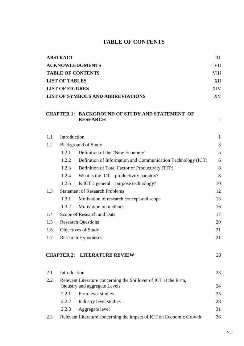
TABLE OF CONTENTS

ABSTRACT III

ACKNOWLEDGMENTS ...........................................................................................VII

TABLE OF CONTENTS ........................................................................................... VIII

LIST OF TABLES .......................................................................................................XII

LIST OF FIGURES ................................................................................................... XIV

LIST OF SYMBOLS AND ABBREVIATIONS ...................................................... XV

1 CHAPTER 1: BACKGROUND OF STUDY AND STATEMENT OF

RESEARCH .......................................................................................... 1

1.1 Introduction 1

1.2 Background of Study 3

1.2.1 Definition of the “New Economy” .......................................................... 5

1.2.2 Definition of Information and Communication Technology (ICT) ........ 6

1.2.3 Definition of Total Factor of Productivity (TFP) .................................... 8

1.2.4 What is the ICT – productivity paradox? ................................................ 8

1.2.5 Is ICT a general – purpose technology? ................................................ 10

1.3 Statement of Research Problems 12

1.3.1 Motivation of research concept and scope ............................................ 13

1.3.2 Motivation on methods ......................................................................... 16

1.4 Scope of Research and Data 17

1.5 Research Questions 20

1.6 Objectives of Study 21

1.7 Research Hypotheses 21

2 CHAPTER 2: LITERATURE REVIEW ................................................................. 23

2.1 Introduction 23

2.2 Relevant Literature concerning the Spillover of ICT at the Firm,

Industry and aggregate Levels 24

2.2.1 Firm level studies .................................................................................. 25

2.2.2 Industry level studies............................................................................. 28

2.2.3 Aggregate level ..................................................................................... 31

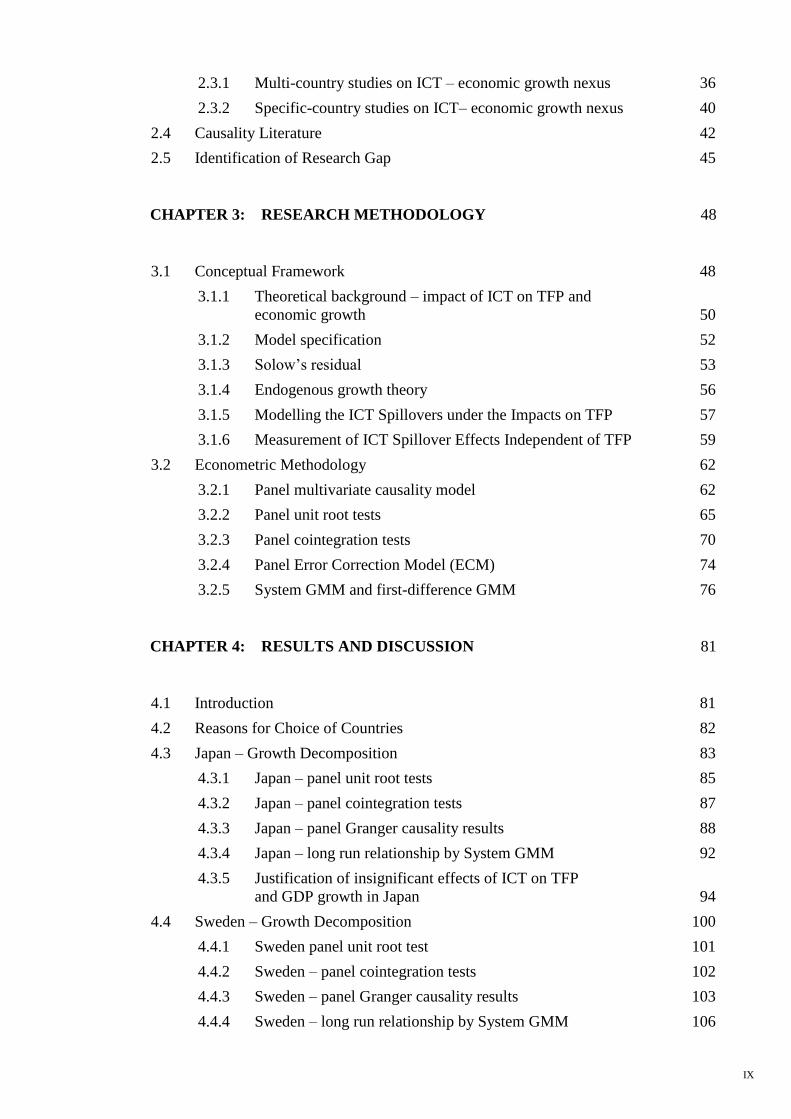
2.3 Relevant Literature concerning the impact of ICT on Economic Growth 36

IX

2.3.1 Multi-country studies on ICT – economic growth nexus...................... 36

2.3.2 Specific-country studies on ICT– economic growth nexus .................. 40

2.4 Causality Literature 42

2.5 Identification of Research Gap 45

3 CHAPTER 3: RESEARCH METHODOLOGY ..................................................... 48

3.1 Conceptual Framework 48

3.1.1 Theoretical background – impact of ICT on TFP and

economic growth ................................................................................... 50

3.1.2 Model specification ............................................................................... 52

3.1.3 Solow’s residual .................................................................................... 53

3.1.4 Endogenous growth theory ................................................................... 56

3.1.5 Modelling the ICT Spillovers under the Impacts on TFP ..................... 57

3.1.6 Measurement of ICT Spillover Effects Independent of TFP ................ 59

3.2 Econometric Methodology 62

3.2.1 Panel multivariate causality model ....................................................... 62

3.2.2 Panel unit root tests ............................................................................... 65

3.2.3 Panel cointegration tests ........................................................................ 70

3.2.4 Panel Error Correction Model (ECM)................................................... 74

3.2.5 System GMM and first-difference GMM ............................................. 76

4 CHAPTER 4: RESULTS AND DISCUSSION ........................................................ 81

4.1 Introduction 81

4.2 Reasons for Choice of Countries 82

4.3 Japan – Growth Decomposition 83

4.3.1 Japan – panel unit root tests .................................................................. 85

4.3.2 Japan – panel cointegration tests ........................................................... 87

4.3.3 Japan – panel Granger causality results ................................................ 88

4.3.4 Japan – long run relationship by System GMM.................................... 92

4.3.5 Justification of insignificant effects of ICT on TFP

and GDP growth in Japan ..................................................................... 94

4.4 Sweden – Growth Decomposition 100

4.4.1 Sweden panel unit root test ................................................................. 101

4.4.2 Sweden – panel cointegration tests ..................................................... 102

4.4.3 Sweden – panel Granger causality results ........................................... 103

4.4.4 Sweden – long run relationship by System GMM .............................. 106

X

4.4.5 Justification of significant effects of ICT on TFP

and GDP growth in Sweden ................................................................ 108

4.5 Australia – Growth Decomposition 110

4.5.1 Australia – panel unit root tests ........................................................... 112

4.5.2 Australia – panel cointegration tests ................................................... 113

4.5.3 Australia – panel Granger causality results ......................................... 114

4.5.4 Australia – long run relationship by System GMM ............................ 116

4.5.5 Justification of significant effects of ICT on TFP

and GDP growth in Australia .............................................................. 119

4.6 Finland – Growth Decomposition 121

4.6.1 Finland – panel unit root tests ............................................................. 124

4.6.2 Finland – panel cointegration tests ...................................................... 125

4.6.3 Finland – panel Granger causality results ........................................... 126

4.6.4 Finland – long run relationship by System GMM .............................. 129

4.6.5 Justification of insignificant effects of ICT on TFP

and GDP growth in Finland ................................................................ 131

4.7 Denmark – Growth Decomposition 135

4.7.1 Denmark – panel unit root tests .......................................................... 137

4.7.2 Denmark – panel cointegration tests ................................................... 138

4.7.3 Denmark – panel Granger causality results ........................................ 140

4.7.4 Denmark – long run relationship by System GMM ............................ 142

4.7.5 Justification of insignificant effects of ICT on GDP

growth in Denmark ............................................................................. 144

5 CHAPTER 5: AGGREGATE LEVEL RESULTS AND ANALYSIS ................ 147

5.1 Introduction 147

5.2 Asia-Pacific and European Growth Decomposition 148

5.3 Unit Root Tests for Asia-Pacific and European Countries 152

5.4 Panel Cointegration Tests for Asia-Pacific and European Countries 154

5.5 Panel Granger Causality Results for Asia-Pacific and European

Countries 155

5.6 Panel Long run Relationship by Using System GMM for Asia-Pacific

and European Countries 159

5.7 Justification of insignificant effects of ICT on GDP growth in EU

and Asia-Pacific countries 165

6 CHAPTER 6: CONCLUSION, POLICY IMPLICATIONS,

AND FURTHER RESEARCH ........................................................ 172

XI

6.1 Introduction 172

6.2 Main Findings of Industrial Level Data 174

6.2.1 Japan .................................................................................................... 174

6.2.2 Sweden ................................................................................................ 176

6.2.3 Australia .............................................................................................. 178

6.2.4 Finland ................................................................................................ 179

6.2.5 Denmark .............................................................................................. 181

6.3 Comparative Results between Asia-Pacific and EU Countries 183

6.4 Policy Implications and Further Studies 191

6.4.1 For Asian countries, the suggestions for policy implications ............. 193

6.4.2 For European countries, the suggestions for policy implications ....... 195

REFERENCES 199

APPENDIX A-Panel Unit Root Tests, All Individual Countries ............................ 213

APPENDIX B-Panel Co-integration Tests, All Individual Countries .................... 214

XII

LIST OF TABLES

Table 1-1. Descriptive of variables used in aggregate level section 17

Table 1-2. Six top ranking of ICT development index (IDI) among

EU and Asia-Pacific countries 18

Table 1-3. Descriptive of variables used in industrial level section 18

Table 1-4. List of industries 19

Table 2-1. Summary of empirical studies on ICT spillover effects

on TFP at the firm, industry and national levels 25

Table 2-2. Summary of multi-country and specific-country

empirical studies on ICT – economic growth nexus 37

Table 3-1. Panel unit root test classification 66

Table 4-1. Six top ranking of ICT development index (IDI)

among EU and Asia-Pacific countries 83

Table 4-2. Japan growth decomposition 84

Table 4-3. Japan panel unit root tests 86

Table 4-4. Kao’s residual cointegration test results 87

Table 4-5. Pedroni’s (2004) residual cointegration test 88

Table 4-6. Panel causality test results for Japan 89

Table 4-7. Panel industries direction of causality in the

short run and long run, Japan 91

Table 4-8. Long run panel data estimators for industries, Japan 93

Table 4-9. Sweden’s growth decomposition 100

Table 4-10. Panel unit root tests, Sweden 102


Table 4-12. Pedroni's (2004) panel cointegration test 103

Table 4-13. Panel short run and long run causality test results, Sweden 104

Table 4-14. Panel industries causal direction in short run

and long run, Sweden 105

Table 4-15. Long run panel data estimators for industries, Sweden 107

Table 4-16. Australia growth decomposition 111

Table 4-17. Panel unit root tests, Australia 112



Table 4-20. Panel causality test results, Australia 115

Table 4-21. Panel industries direction of causality in short run

and long run, Australia 115

Table 4-22. Long run panel data estimators for industries, Australia 117

Table 4-23. Finland growth decomposition 122

Table 4-24. Finland panel unit root tests 124


Table 4-26. Pedroni’s (2004) residual cointegration test results 125

Table 4-27. Panel causality test results, Finland 127


and long run, Finland 128

XIII

Table 4-29. Long run panel data estimators for industries, Finland 130

Table 4-30. Denmark growth decomposition 135

Table 4-31. Denmark panel unit root tests 138



Table 4-34. Panel causality test results, Denmark 140

Table 4-35. Panel industries causality direction in short run

and long run, Denmark 141

Table 4-36. Long run panel data estimators for industries, Denmark 143

Table 5-1. Six top ranking according to the ICT development

index (IDI) among EU and Asia-Pacific countries 147

Table 5-2. Asia-Pacific growth decomposition 149

Table 5-3. European growth decomposition 150

Table 5-4. Asia-Pacific and European countries, panel unit root tests 153

Table 5-5. The Kao residual cointegration test results 155

Table 5-6. Panel causality test results, Asia-Pacific countries 156

Table 5-7. Panel causality test results, EU countries 157


and long run, Asia-Pacific 158


and long run, EU 159

Table 5-10. Long run panel data estimators for Asian and

European countries 162

Table 6-1. Overall industrial level results, significant effects

of ICT on EG and TFP 179

Table 6-2. Overall industrial level results, insignificant effects


Table 6-3. Overall Aggregate level results, insignificant effects


XIV

LIST OF FIGURES

Figure 1-1. Trend of "New Economy" 6

Figure 1-2. Worldwide investment by the private sector in

infrastructure-projects 14

Figure 2-1. Classification of literature review 23

Figure 3-1. Conceptual framework 48

Figure 3-2. Research methodology 49

Figure 3-3. Econometric framework 50

Figure 4-1. Contribution of ICT, non-ICT, Labour, and TFP

to value added 85

Figure 4-2. Average growth rate of value added for each industry, Japan 95

Figure 4-3. Ranking trends in major international ICT indices 97

Figure 4-4. Utilization in Public Sector for Japan, 2010 97

Figure 4-5. Contribution of ICT Capital Services to GDP Growth

(annual %) 98

Figure 4-6. Total Factor Productivity Growth (annual %) 99

Figure 4-7. Contribution of ICT, non-ICT, Labour, and TFP to

value added 100

Figure 4-8. Average growth rate of value added for each industry,

Sweden 109

Figure 4-9. Contribution of ICT, non-ICT, Labour, and TFP to

value added 111


Australia 119

Figure 4-11. Contribution of ICT, non-ICT, Labour, and TFP

to value added growth 123


Finland 133

Figure 4-13. Contribution of ICT, non-ICT, Labour, and TFP to value 136


Denmark 145

Figure 5-1. Growth decomposition for six top ranking of ICT 150

Figure 5-2. Growth decomposition for six top ranking of ICT 151

XV

LIST OF SYMBOLS AND ABBREVIATIONS

ICT Information Communication Technology

IT Information Technology

GPT General Propose Technology

TFP Total Factor Productivity

Non_ICT Non Information Communication Technology

EG Economic Growth

ITU International Telecommunication Union

CT Communications Technology

DSL Digital Subscriber Line

Α Elasticities

A Solow Residual

ATMs Automated Teller Machines

GDP Gross Domestic Product

WBI World Bank Indicators

IDI ICT Development Index

OECD Organisation for Economic Co-operation and Development

Countries

EDI Electronic Data Interchange

APL Labour Productivity

BLS Bureau of Labour Statistics

R&D Research and Development

LSDV Least Square Dummy Variables

PMG Pooled Mean Group

MG Mean Group

DFE Dynamic Fixed Effect

GMM Generalised Moment of Method

OPEC Organization of the Petroleum Exporting Countries

PDOLS Panel Dynamic Ordinary Least Squares

OLS Ordinary Least Squares

XVI

3SLS Three-stage Least Squares

Gi Growth Gap

PROF Productivity in Frontier Group Countries

PROI Productivity Flowers Group Countries

PROi Labour Productivity

CEE Central and Eastern European

ECT Error Correction Term

ECM Error-Correction Model

VECM Vector Error Correction Model

Uit Error Term

Yit Value Added Growth

β1, β2, β3 Elasticities of the Production Resources

ICT_prod ICT-producing Industries

ICT_use ICT Using Industries

K ICT Information Communication Technology Capital

K non-ICT Non Information Communication Technology Capital

Lit Labour Capital

Ictim ICT Goods Imports

Ptn Patent Applications, Non-residents

Ptr Patent Applications, Residents

Terit School Enrolment, Tertiary

Ht High-Technology Exports

Upl Unemployment

Exp Exports of Goods and Services

Imp Imports of Goods and Services

VAR Vector Auto-Regression

DF Dickey-Fuller

ADF Augmented Dickey-Fuller

CADF Cross-sectional Augmented Dickey-Fuller

PP Phillips-Perron

XVII

AIC Akaike Information Criterion

LM Lagrange Multiplier

ηi Country

δi Industry

eit Estimated Residuals

Fixed Effects for Each Industry or Country

Coefficients of the Lagged Dependent Variables

Coefficients of Current and Lagged Independent Variables

T Time Observations

N Cross-sectional Observations

ARDL Autoregressive Distributed Lag Model

ASEAN Association of Southeast Asian Nations

IVs Instruments

NICTA Australia's Information and Communications Technology Research

Centre of Excellence

IPS Im, Pesaran & Shin (1997) Test

KT Korea Telecom

C&W Cable and Wireless Services

CIs Cluster Initiatives

http://en.wikipedia.org/wiki/Information_and_Communications_Technology

1

1 CHAPTER 1: BACKGROUND OF STUDY AND STATEMENT OF

RESEARCH

1.1 Introduction

In recent years, one of the most essential concerns of economists is whether the

accumulation of Information Communication Technology (ICT) capital positively

contributes to the growth in income and productivity in various countries. This

uncertainty has prompted vigorous debate among economists. One camp has argued that

the improvement of ICT is among a series of positive provisional shocks, thus, having

no effect on expansion, while another camp claimed that it leads to increasing growth

prospects as it has produced a fundamental change in the economy.

ICT is a kind of technology with broad access in many parts and has produced the

amplitude of complementary production. This technology can further enhance its

productivity via specialisations and economies of scale. Today, around 90 per cent of

the world population have been subscripted to mobile cellular networks (ITU1, 2012).

According to the International Telecommunication Union’s (ITU) estimations, net user

penetration had covered 21 per cent of the population in developing countries, 71 per

cent in developed countries and a mere 9.6 per cent in African countries by the end of

2012. It has been vastly acknowledged that ICT is increasingly influential in both social

and economic developments. Using the Internet and access to broadband are in fact,

akin to using basic substructures like roads and electricity; thus it is regarded as a

general-purpose technology.2

Generally, the empirical investigation of economic growth and productivity usually

distinguishes three impacts of ICT. The first effect is capital deepening as a result of

investment, which, in turn, helps raise productivity and GDP growth. The second effect

1ITU, ICT data and statistics, http://www.itu.int/ITU-D/ict/publications/world/world.html 2See more information in section 1.2.5

2

is efficiencies of capital and labour or total factor productivity (TFP), which relates to

quick technological advancement in the production of ICT goods and services. This

consequently leads to increased return to ICT-producing sectors. Finally, a similar

impact can also be attributed to the wider use of ICT throughout the economy as firms

augment their general efficiency.

Furthermore, the increased use of ICT may contribute to network impacts by means of

lowering transaction costs and encouraging speedier modernisation. Likewise, this

improves the TFP. Such effects can be examined at diverse stages of analysis, i.e. with

individual firm data, macroeconomic data or data at the industry level. The industry and

aggregate level evidence supply cooperative insights concerning the effects of ICT,

particularly on value added growth. However, it also raises questions concerning under

which conditions does ICT growth become effective in enhancing value added growth

for industries. Despite substantial investment in ICT, the industry and aggregate level

evidence indicates extremely limited impact of technology on the productivity and

growth in most countries. One probability is that computers remain invisible in the

productivity data of many countries. For example, the Solow’s productivity paradox 3

could have remained unsolved for some countries (Pilat, 2004; Solow, 1987). This

productivity paradox will be discussed in detail in the subsequent sections.

Industrial level data may assist in explaining why ICT growth has led to greater

economic effect. Certainly, it could indicate the impact on the contributory factors that

cannot be observed at the aggregate level. In addition, the industrial level data can also

make clear the competitive and dynamic effects that may come with the broadening of

ICT. One example is the entrance of new industries and the exit of some failed

3The most common 'explanation' for the Solow paradox is offered by Jack E. Triplett (1999). It contains separate sections of evaluating for each position, and can be found at this address: http://www.jstor.org/stable/pdfplus/136425.pdf?acceptTC=true. In

addition, we have completed the Solow residual explanation in chapter 3.

http://www.jstor.org/stable/pdfplus/136425.pdf?acceptTC=true

3

industries in the short and long run in contrast with industrial level and aggregate level

evidence, which provides considerable information for countries affected by ICT-

productivity, particularly in terms of their productivity and value added growth. Such

evidence may also determine the consistency of the results on the aggregate and

industry levels.

Industrial level evidence pertaining to ICT is now available in many developed

countries (Pilat, 2004). This is attributed to the progress of the countries in the statistical

development of ICT technologies, particularly on its various uses in the economy.

Additionally, most Asian and several European countries are now able to collect

industry level information on ICT and TFP contribution to value added. Combining

these aggregate and industrial sources would be helpful in establishing new links

between industry and macroeconomic performance, provided that the database is

representative or includes a large portion of the economy.

1.2 Background of Study

The contribution of Information Communication Technology (ICT) to the resurgence of

value added growth, as experienced in many developed countries, has attracted the

attention of two groups – the economists and the policymakers. The discovery of

relationships among economic growth, ICT, and Total Factor Productivity (TFP)

growth has prompted a series of economic researches using different approaches.

Among the earliest discoveries were the Solow growth model, Solow productivity

paradox4 and endogenous growth model.

The Paradox refers to economics that present negative or negligible productivity growth

rates despite the evidence of large ICT and innovation investments in the country. This

has been demonstrated in different countries and industries in recent decades. Hence,

4The Solow residual is explained in detail in chapter 3. See more information in chapter 3, Section 3.1.3.

4

ICT has been found to play both direct and indirect roles in the economic growth

process. It is also believed to have an effect on ICT-producing, using industries and

enhance productivity via its application (Badescua & Garce´s-Ayerbe, 2009). The

massive and clear contribution of ICT to TFP and economic growth rose to an

unprecedented level in 1987, when Robert Solow asserted that its contribution to

organisational works remained vague or insignificant despite strong investments by the

US companies. The reasons behind this paradox are further explained in the next

sections.

The improvement of the endogenous growth models, which were generated by the

research results of Romer (1986, 1990) and Lucas (1988) in the late 1980s, has

encouraged further investigations on endogenous factors that influence economic

growth. Lucas (1993), for instance, mentioned that the main engine for economic

growth has been the accumulation of human capital. Therefore, human resources

constitute a productive and dynamic stock. Each individual, by extension, is not only a

factor of production, but also a life-long partner, a decision-maker and a trainable team-

member.

Therefore, any work environment that enables human resources to access more ICT will

enhance their communication abilities and learning productivity, which, in turn, will

lead them to effectively become bigger in the existing stock of human factors. This kind

of improvement is expected to affect economic growth significantly and it is for this

reason that ICT investment attracts widespread attention among researchers. Among the

results arising from the ICT revolution are the improvements in labour skills, the

increased level of broad-based education and the motivation to consume. Consequently,

an improved utilisation of ICT and TFP is encouraged in line with Solow’s argument

that information access will improve faster if barriers are relaxed and investments are

encouraged.

5

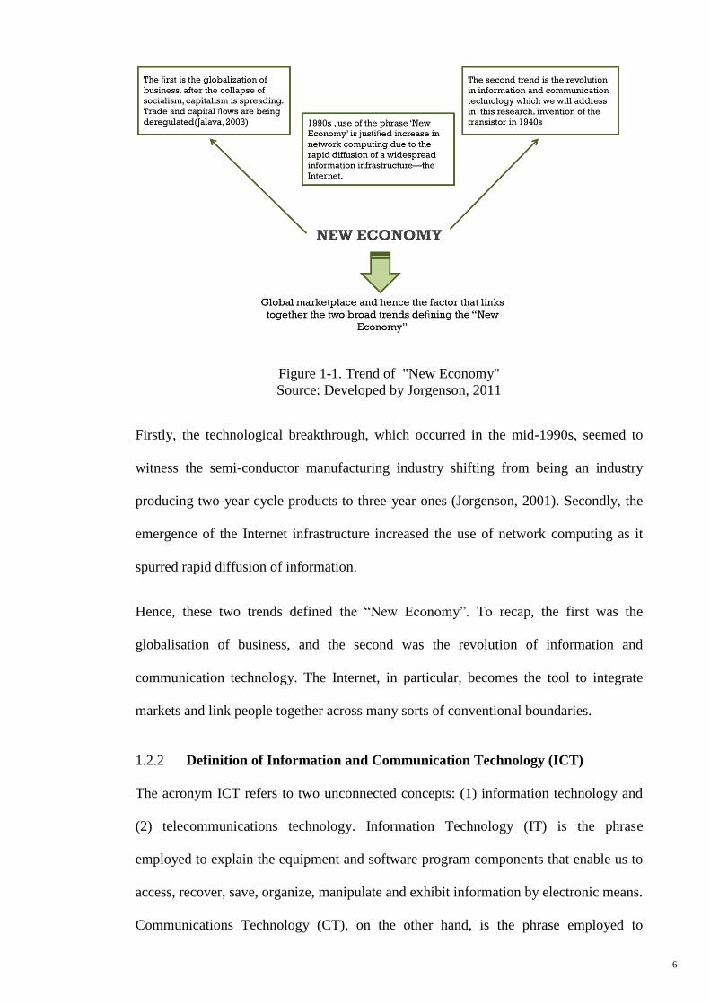
1.2.1 Definition of the “New Economy”

The “New Economy” is a well-defined concept. The term was established by the

business press to describe a couple of wide trends around the world economy (Shepard,

1997). The first was business globalisation, which referred to the breakdown of

socialism when capitalism spread around the world. This trend was market-driven with

further trade deregulation trading then capital flows. Hence, multinational commerce

and investment have assumed a significantly larger role in every country’s economic

plans compared to fifteen to twenty years ago (Jalava, 2003).

The second trend referred to the revolution of information and communication

technology (ICT), which is the focus of this study. Such an advancement was driven by

many forces, notably: (1) the immediate progressiveness in quality, (2) the fast fall in

the prices of ICT products and software, (3) the convergence in telecommunications

and computing techniques, and (4) the accelerated enhancement in network computing.

This revolution seems to have continued ever since the advent of the transistor in the

1940s.

Henceforth, the price of computers declined sharply compared to fifty years ago. All

these have supposedly justified what the “New Economy” is. Consider the following

attributes as shown in Figure 1-1:

6

Figure 1-1. Trend of "New Economy"

Source: Developed by Jorgenson, 2011

Firstly, the technological breakthrough, which occurred in the mid-1990s, seemed to

witness the semi-conductor manufacturing industry shifting from being an industry

producing two-year cycle products to three-year ones (Jorgenson, 2001). Secondly, the

emergence of the Internet infrastructure increased the use of network computing as it

spurred rapid diffusion of information.

Hence, these two trends defined the “New Economy”. To recap, the first was the

globalisation of business, and the second was the revolution of information and

communication technology. The Internet, in particular, becomes the tool to integrate

markets and link people together across many sorts of conventional boundaries.

1.2.2 Definition of Information and Communication Technology (ICT)

The acronym ICT refers to two unconnected concepts: (1) information technology and

(2) telecommunications technology. Information Technology (IT) is the phrase

employed to explain the equipment and software program components that enable us to

access, recover, save, organize, manipulate and exhibit information by electronic means.

Communications Technology (CT), on the other hand, is the phrase employed to

7

describe the devices, infrastructure, and software whereby information can be obtained

and accessed (for example, phones, faxes, modems, digital networks, and DSL lines).

ICT is consequently the result of the convergence of the IT and CT. One initial instance

of ICT convergence is the crossing of the photocopy machine and telephone, leading to

the creation of the fax. Above all, the clearest example in this area is the convergence of

the computer and telephone, which resulted in the upsurge of the Internet.

In this study, we employ the definition of ICT by EUKLEMS (2010). Classification of

ICT capital based on EUKLEMS databases are derived into three types; namely,

communication equipment, computing equipment and software. Five core indicators on

ICT infrastructure and access are introduced by the ITU, as part of a much larger

collection of telecommunication indicators, Internet users, mobile-cellular telephone

subscription, fixed telephone lines, fixed (wired)-broadband subscription and mobile-

broadband (wireless) subscriptions.

For ICT assets, the gross rate of earnings is generally above other assets. This

demonstrates the fast pace obsolescence of ICT assets. The rate of depreciation reveals

the proportional loss of an asset’s value due to the aging process, which includes not

only the ageing influence but also the value change required by an increase or decline of

the asset price, and even revaluation. In the present format, depreciation is a key

component for the derivation of monitors of value-added. It determines income, net of

the resources, which may have to be allocated to persevere with ICT and non-ICT

capital services intact. Value-added follows the approach of disposable income for

consumption. While not a suitable point of leaving for modelling producer behaviour, it

offers a platform for the welfare point of view of economic growth. The particular

attraction in this research is the impact of ICT contribution on the growth rate through

the volume change in depreciation, since the latter is caused mostly by how much the

volume changes in value-added (Colecchia & Schreyer, 2002).

8

1.2.3 Definition of Total Factor of Productivity (TFP)

One approach to consider the output of an economic system in which inputs are

transformed, is through its production functions. This approach applies the econometric

technique to relay on the output of a firm, industry, or economy to the inputs often

noted as labour and capital. In the productivity research literature, the Cobb-Douglas

functional form is pervasive. This production function has also been broadly used in

earlier studies concerning the impact of ICT on the performance at the firm, industry

and national level (Howitt, 1998). Therefore, we assume a Cobb-Douglas aggregate

production function as follows:

(1.1)

Y = A f (K, L) = A Kα

L 1-α

where ‘Y’ is output or GDP, ‘K’ is the aggregate capital stock that could be decomposed

to ICT and non-ICT capital, ‘L’ is the labour force, and 0<α<1 is the parameter of

output share, demonstrating the elasticities of the production factors . ‘A’ has been taken

to be just a Solow5 residual or the part of an economic factor of productivity that

remains ‘unexplained’. Using the production function from equation (1.1), ‘A’ can be

derived as:

(1.2)

A = Y / (KαL

1-α)

However, the endogenous growth theory challenges the conventional concept and

started to call ‘A’ as TFP. Now it becomes the engine of economic growth (Aghion &

Howitt, 1997).

1.2.4 What is the ICT– productivity paradox?

Robert Solow stated that “computers were everywhere but in the productivity statistics”

due to the studies that were conducted in the 1970s and the 1980s on the effects of

5The Solow residual has been explained in detail in chapter 3, section 3.1.3.

9

investment in ICT on productivity that revealed either negative or zero impact (Solow,

1987). Some evidence was found by recent studies concerning the considerable impact

of ICT capital on the labour productivity, as compared to other forms of capital, which

seemed to suggest that either TFP growth is positively impacted by the ICT or that ICT

investments might have a spillover effect. Recent work on some specific OECD

countries, such as the United States and Australia have categorically shown how total

factor productivity and labour are enhanced by ICT (Gretton, Gali, & Parham, 2004).

In the last decade, there have been studies that have identified a number of factors that

essentially contribute to the productivity paradox. Firstly, in the productivity statistics,

there were some benefits of ICT that were not identified. Although most of the ICT

investment is done in the service sector of an economy, there are difficulties in

measuring the productivity in this sector. For example, the introduction of Automated

Teller Machines (ATMs), which has improved the convenience of financial services is

only looked upon as advancement in the financial services quality in countries. Similar

problems plague other activities, such as health services, insurance and business

services. Although in some sectors, as well as in some EU countries, progress has been

made to improve the measurement, it remains a pivotal problem in judging the overall

effect that ICT has on performance, especially in different countries (Triplett, 1999).

Secondly, it takes a considerable amount of time for the benefits of ICT use to emerge,

making it hard to find evidence on ICT's impact. It is the same case with other key

technologies; electricity is a good example of this. Often the dispersal of new

technology is quite slow and it mostly takes a long time for the firms to adjust to all of

them, e.g. in inventing or executing superior business procedures changing

organisational arrangements or upgrading of the workforce. Furthermore, if it is

assumed that TFP is raised by ICT, partly through the means of the networks that it

provides, time is required for a network to be built that is large enough to have an

10

impact on the economy. However, these effects have not been seen at equal levels in all

the countries, and it is more pronounced in the United States compared to other

countries. This suggests that other countries are still in the process of adjustment to the

dispersal of ICT.

Thirdly, at the firm level, the attempts made to measure the effect of ICT in the early

studies were actually established based on a small sample size of companies relative to

the other studies, which were drawn from private sources. For instance, if ICT only had

a small impact on performance, most probably only slight evidence would be found by

such studies due to the econometric “noise”, through which it can get lost. Another

possibility is that the samples might not be representative, or the poor quality of the

data. Furthermore, several studies have implied that it is important that there should be a

distinction between the activities when the analysis is carried out, as the impact that ICT

has on economic performance might differ from one activity to another. The studies that

are most likely to find an impact of ICT are those that cover several industries and also

have a large sample of official data, unlike the earlier studies. In recent years, a great

deal of progress has been recorded in measuring ICT investment and the dispersal of

ICT technologies, which implies that the series of data that is available is of greater

quality and broader, and is more robust relative to the previous data.

1.2.5 Is ICT a general – purpose technology?

It is commonly argued that ICT is a “special” technology that affects a multitude of

sectors and economic activities by making them productive. For this reason, a narrow

definition of ICT investment would not capture the true impact of ICT on the economy.

Often, ICT is considered to be a general-purpose technology (GPT). However, the idea

of ICT representing a GPT is based on concepts associated with ICT investments that

go beyond the notion of conventional capital equipment. In other words, it is perceived

more as an “enabling technology” (Jovanovic & Rousseau, 2005). This may be true as

11

knowledge becomes qualitatively and quantitatively more important than economic

activities.

ICT facilitates communication and creates new knowledge via more efficient

collaboration and information processing. In firms, this property of ICT can often be

observed. Speedier information developing may perhaps enable firms to deal with new

techniques of communicating with providers and arranging distribution platforms. As a

result, processes can be reorganised and streamlined, which reduce capital needs

through better utilisation of equipment and further reduction of inventories or space

requirements. Increased communication reduces coordination costs and the number of

supervisors required. A more timely and widespread transfer of information enables

better decision-making and reduces labour costs (Arvanitis & Loukis, 2009; Atrostic,

Boegh-Nielsen, Motohashi, & Nguyen, 2004; Gilchrist, Gurbaxani, & Town, 2001).

Lower communication and replication costs allow businesses to innovate by offering

new products (Brynjolfsson & Saunders, 2009). Scholars interested in transaction costs

consider communication technologies as capable of lowering the fixed costs of

acquiring information and the variable costs of participating in the markets (Norton,

1992). The notion of new ideas or techniques that influence the economy on a broad

basis was first published by Bresnahan and Trajtenberg (1995) who coined the phrase of

GPTs. The main characteristics of GPT are as follows:

i) Applicability across a broad range of uses – “pervasiveness”;

ii) Wide scope for improvement, experimentation and elaboration, continuously

reducing costs – “improvement”; and

iii) Facilitating further product and process innovations – “innovation spawning”.

In the case of spillover effects from ICT, its capacity to serve as a GPT is reflected in

the dramatic decrease in ICT prices, leading to a substitution of ICT equipment for less

productive assets (Jorgenson & Nomura, 2005).

12

Regarding the surge in the United States productivity during the period of the "New

Economy", it was a consensus that strong IT investment was perceived as a driving

force, where much of it originated from the ICT-producing sectors. Nevertheless, there

is at least some indication that the efficiency gained from it has been spilling over to

other industries that heavily use these new technologies as well. It is this characteristic

that makes ICT likely to be a GPT, since, ultimately, computers and linked ICT

equipment are expected to be utilised in most sectors of the economy as digitisation

continues. Although it might be reasonable to claim that productivity gains from ICT

can be found all around in daily business life, quantifying the spillover effect is

difficult, as they are hard to isolate (Kretschmer, 2012).

This study intends to benefit policymakers by highlighting important accomplishments

as an attempt to present quantitative indicators for measuring the role of ICT on GDP

growth.

Bresnahan and Trajtenberg (1995) presented a line of study offering ICT as a general-

purpose technology (GPT), which was based on the natural potential for ‘technical

improvements’, ‘pervasiveness’, and ‘innovation complementarities’, thus, contributing

more towards rising returns-to-scale (Brynjolfsson & Hitt, 2000). Similarly, David

(1990) claimed that ICT has to be seen as widespread and general-purpose technologies

that are certain to spread in the economic system and strengthen productivity growth,

albeit with a lag. The exclusive value of ICT is the fact that by enabling essential

changes in business processes and organizational structures, it may augment the TFP.

1.3 Statement of Research Problems

The work started by Romer (1986, 1990) and Lucas (1988) in the late 1980s concerning

the development of the endogenous growth models kick started many empirical studies

to explore and study the endogenous factors that are the determinants of economic

growth. Accumulation of human capital has been consistently found across the studies

13

to play a significant role as ‘‘the primary engine of growth’’ (Lucas, 1993). However,

human capital is found to be quite a productive stock and dynamic as opposed to being

static, as it is not as if each individual is just an inert worker, inasmuch as each

individual is also a team-worker, a decision-maker, and a life-long learner. If the

working conditions are improved by giving better access to information to people, and,

at the same time, facilitating their communication abilities and learning productivity,

then the current stock of human capital is effectively enlarged, while also enhancing its

use.

Hence, there should be a positive impact due to these types of improvement on the

economic growth. Given the preference to demand over supply, it is argued by Quah

(2002) that improvements are fostered in consumer sophistication, improved level of

broad-based education and labour skills through the revolution of Information and

Communication Technology (ICT). In turn, this raises labour productivity and boosts

the greater usage of technology, and, as a consequence, ‘‘drives economic growth, one

way or another’’ (Quah, 2002). It is argued by Levine (1997) that by reducing the

obstacles to information access, ICT is considered as a significant driver and encourages

increased investment, which, in turn, promotes faster growth.

1.3.1 Motivation of research concept and scope

Until today, economists have fundamentally looked at the effect of ICT on economic

growth and productivity within a neoclassical framework of ‘unilateral relationship’, in

which ICT is supposed to correspond to other types of capital (Dimelis & Papaioannou,

2011; Inklaar, O'Mahony, & Timmer, 2005; Van Ark, Inklaar, & McGuckin, 2003).

This approach, however, is relatively restrictive in fully capturing the impact of ICT.

For this reason, we will conduct our econometric model by bypassing the assumptions

of growth.

14

We will establish not only the contribution of ICT growth to productivity development,

but to TFP, labour and non-ICT output growth as well. This we hope will fill the

knowledge gap on causal relationships between the contribution of ICT, non-ICT,

labour, Total Factor Productivity (TFP) and the value added growth rate. Moreover,

there seems to be relatively very limited empirical studies pertaining to the impact of

ICT on economic growth at the industrial and aggregate levels, specifically in the top

ICT developed Asia-Pacific and European countries. There are inequalities in growth

across countries and industries, which can be explained by the economic factors.

However, what role does ICT play regarding this phenomenon?

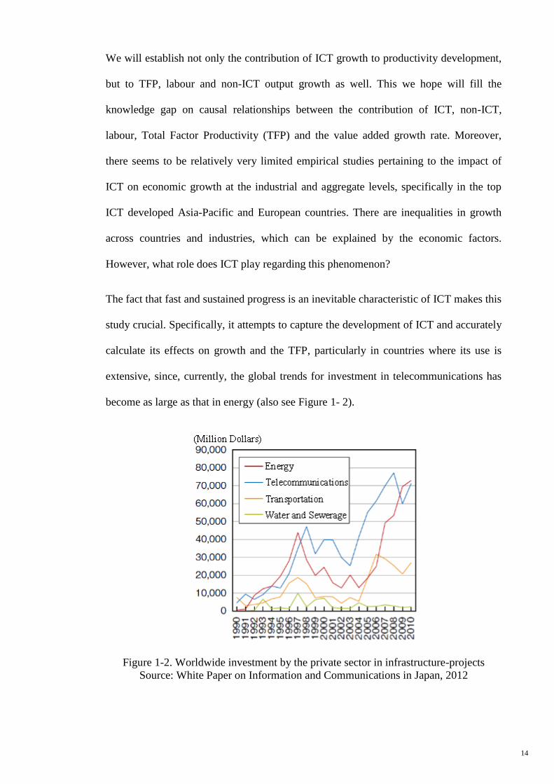
The fact that fast and sustained progress is an inevitable characteristic of ICT makes this

study crucial. Specifically, it attempts to capture the development of ICT and accurately

calculate its effects on growth and the TFP, particularly in countries where its use is

extensive, since, currently, the global trends for investment in telecommunications has

become as large as that in energy (also see Figure 1- 2).

Figure 1-2. Worldwide investment by the private sector in infrastructure-projects

Source: White Paper on Information and Communications in Japan, 2012

15

The exploratory role of ICT at the sectoral and aggregate levels raises some difficult

questions that we intend to answer by classifying the literature according to the firm,

industry and aggregate levels. The discussion suggests whether aggregate evidence or

industry level data may cause an apparent productivity paradox. Some European

countries besides the Asian countries may have not yet benefited from the spillover

effects that would generate a wedge between the impacts observed on individual

industries and those at the macroeconomic level. According to previous studies, the

results may vary depending on the duration, area, and type of sector involved.

Therefore, the manifesting productivity paradox between a few Asia-Pacific and EU

countries will complete the research chain in this area.

Enhancements in measuring data have performed a significant role in building up the

evidence of the effects of ICT. Most of the previous work with the industrial data on

ICT and productivity was influenced by different data sources. However, sources from

individual countries have a number of methodological drawbacks. Firstly, often, the

data do not represent a fixed sample of industries, indicating the possibility of biased

conclusions being drawn. Furthermore, scientific studies depending on specified sample

of industries will tend to disregard dynamic impacts, just like the entrance of new

players or the demise of existing ones, which might accompany the extent of ICT.

Secondly, the quality and comparability of individual country data sources are

questionable, as they are not necessarily verified by international statistical conventions,

measures or definitions.

Indeed, the benefits of industry level analysis and the aggregate level effects of ICT are

materialised in the form of longitudinal databases in international statistical offices.

Among the first were the databases of the EU KLEMS and World Bank Indicators

(WBI). These databases are more extensive and statistically more representative

samples compared with those available in individual country statistical centres. The

16

availability of such data is imperative given the enormous data for the industry

performance of countries. Furthermore, they allow industries to be tracked over time

and could be correlated to other research and data sources.

1.3.2 Motivation on methods

Most previous studies viewed the association between ICT, TFP and economic

development in different nations or periods. However, essentially, this relationship, fails

to imply a causal relationship, particularly when non-stationary time series variables are

not cointegrated. In particular, the Granger causality test allows us to identify the

directions of causality and establish whether ICT growth results in GDP growth, or vice

versa, and/or whether a spillover effect through TFP growth is present between the two.

This spillover effect of ICT under the endogenous growth framework, particularly in the

aggregate panel data section, is distinguished by employing controlling variables.

However, due to the discriminated sectoral effects of ICT on value added growth,

particularly at the macro-level, we will analyse the pooled mean group using the

generalised method of moment under the growth-accounting framework.

Despite being resource intensive, panel data analysis allows scholars to achieve a deeper

understanding of the effect of ICT contribution on growth. As Kohli and Devaraj (2003)

suggested, using larger samples including cross-sectional or panel data can assess the

impacts of ICT payoff correctly. Such samples can frequently enhance the accuracy of

the econometric analysis, because, through using these data, country (industry) specific

effects can be controllable. Applying this sort of data also permits the researcher to

observe the lag effects of ICT impact. This is an advantage, as ignoring lag effects has

been cited as a factor that contributes to GDP growth (Gholami, Sang-Yong, &

Heshmati, 2006). Using pooled time series studies with cross-sectional also has been

able to answer some specific questions to be answered. For example, we could classify

whether the relationship between variables is in the short or long run.

17

1.4 Scope of Research and Data

The main purpose of this study is to exploit the comprehensive ICT effects on economic

growth with regards to the top ICT developed countries in Asia-Pacific and Europe. To

fulfil this objective, we collected the aggregate level data for the 12 top ranked ICT

countries in both regions from the World Bank Indicator database. Annual data

collected between 1990 and 2011 served as the secondary data. The countries listed in

the EU are Sweden, Iceland, Denmark, Finland, Luxembourg, and Switzerland while

those in the Asia Pacific include Korea (Rep), Hong Kong, New Zealand, Japan,

Australia, and Singapore. At the aggregate level, estimation methods were applied to the

following variables (Table 1-1) as part of the research.

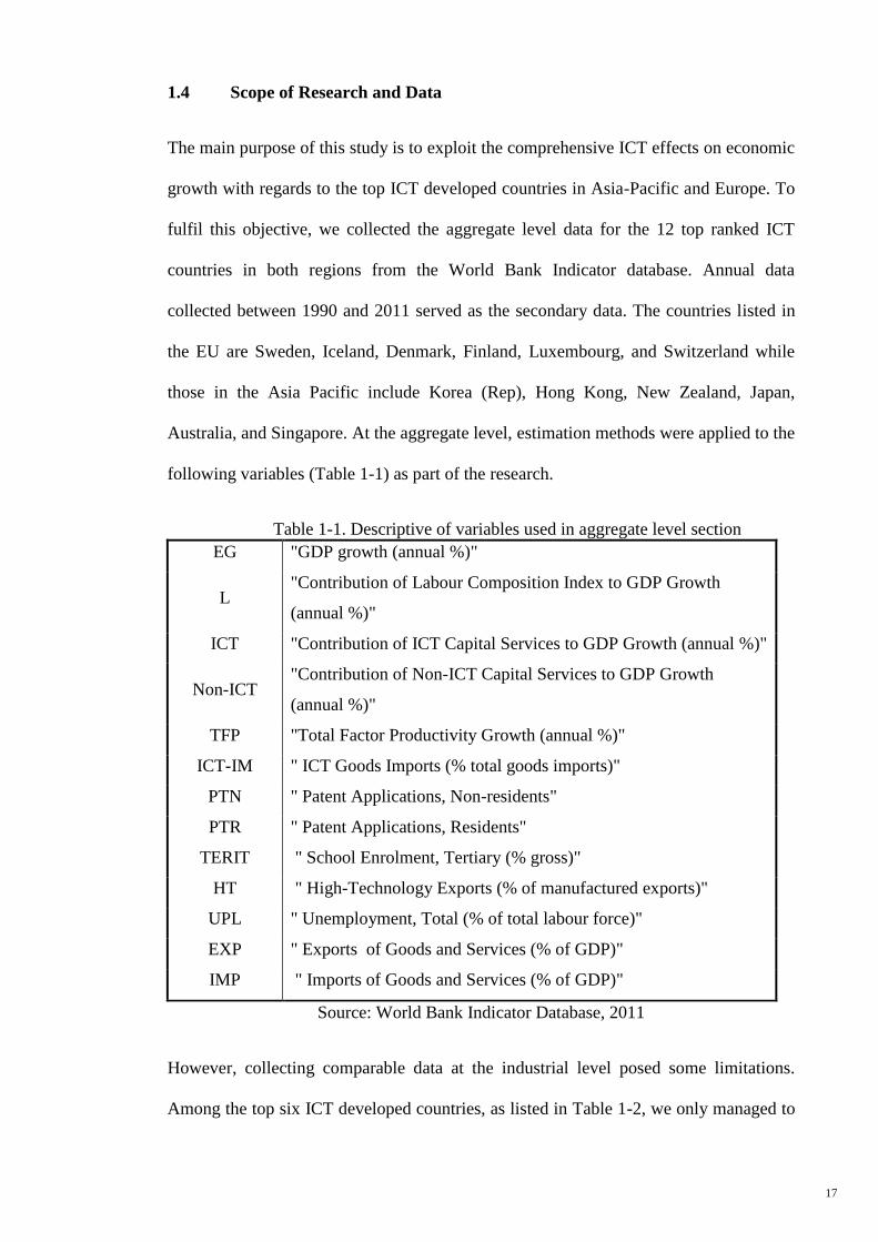
Table 1-1. Descriptive of variables used in aggregate level section

EG "GDP growth (annual %)"

L "Contribution of Labour Composition Index to GDP Growth

(annual %)"

ICT "Contribution of ICT Capital Services to GDP Growth (annual %)"

Non-ICT "Contribution of Non-ICT Capital Services to GDP Growth

(annual %)"

TFP "Total Factor Productivity Growth (annual %)"

ICT-IM " ICT Goods Imports (% total goods imports)"

PTN " Patent Applications, Non-residents"

PTR " Patent Applications, Residents"

TERIT " School Enrolment, Tertiary (% gross)"

HT " High-Technology Exports (% of manufactured exports)"

UPL " Unemployment, Total (% of total labour force)"

EXP " Exports of Goods and Services (% of GDP)"

IMP " Imports of Goods and Services (% of GDP)"

Source: World Bank Indicator Database, 2011

However, collecting comparable data at the industrial level posed some limitations.

Among the top six ICT developed countries, as listed in Table 1-2, we only managed to

18

cover Japan and Australia using the EU KLEMS database. Hence, the industrial level

data was only derived from the unique EU KLEMS database for two reasons. First,

often, individual country data often does not derive from a representative fixed sample

of industries and further suffers from a number of drawbacks in the methodological

parts of the research. This may imply that the results of such studies are biased, and,

hence, may not be comparable. Second, the comparability and quality of individual

country data sources are generally unknown, whereas the data are not essentially

verified by international statistical conventions, procedures or definitions.

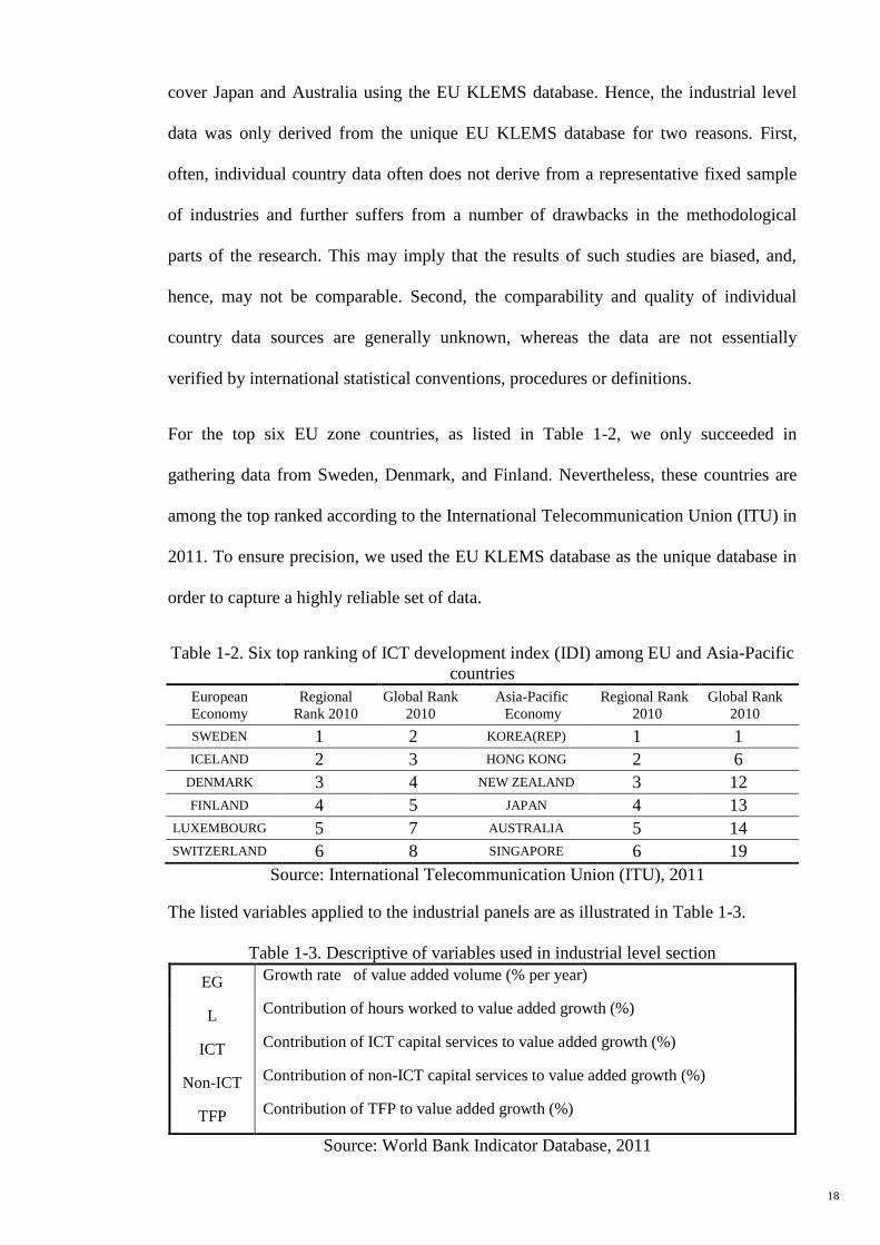
For the top six EU zone countries, as listed in Table 1-2, we only succeeded in

gathering data from Sweden, Denmark, and Finland. Nevertheless, these countries are

among the top ranked according to the International Telecommunication Union (ITU) in

2011. To ensure precision, we used the EU KLEMS database as the unique database in

order to capture a highly reliable set of data.

Table 1-2. Six top ranking of ICT development index (IDI) among EU and Asia-Pacific

countries

European

Economy

Regional

Rank 2010

Global Rank

2010

Asia-Pacific

Economy

Regional Rank

2010

Global Rank

2010

SWEDEN 1 2 KOREA(REP) 1 1

ICELAND 2 3 HONG KONG 2 6

DENMARK 3 4 NEW ZEALAND 3 12

FINLAND 4 5 JAPAN 4 13

LUXEMBOURG 5 7 AUSTRALIA 5 14

SWITZERLAND 6 8 SINGAPORE 6 19

Source: International Telecommunication Union (ITU), 2011

The listed variables applied to the industrial panels are as illustrated in Table 1-3.

Table 1-3. Descriptive of variables used in industrial level section

EG Growth rate of value added volume (% per year)

L Contribution of hours worked to value added growth (%)

ICT Contribution of ICT capital services to value added growth (%)

Non-ICT Contribution of non-ICT capital services to value added growth (%)

TFP Contribution of TFP to value added growth (%)


19

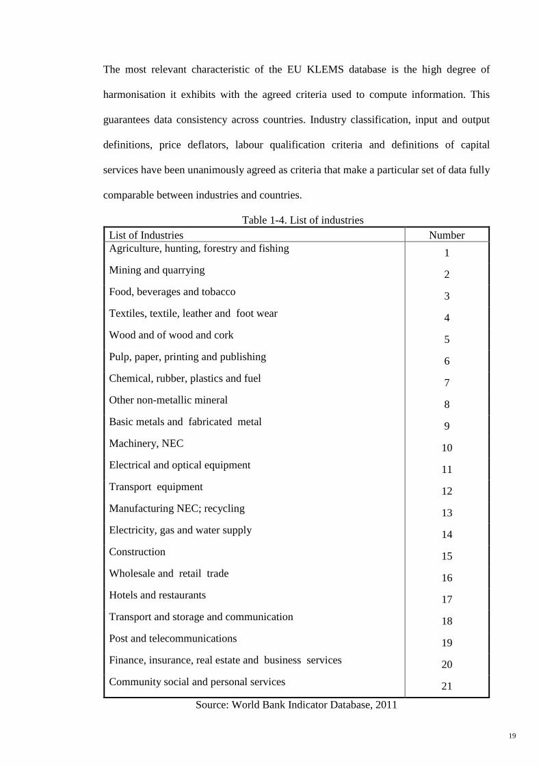
The most relevant characteristic of the EU KLEMS database is the high degree of

harmonisation it exhibits with the agreed criteria used to compute information. This

guarantees data consistency across countries. Industry classification, input and output

definitions, price deflators, labour qualification criteria and definitions of capital

services have been unanimously agreed as criteria that make a particular set of data fully

comparable between industries and countries.

Table 1-4. List of industries

List of Industries Number

Agriculture, hunting, forestry and fishing 1

Mining and quarrying 2

Food, beverages and tobacco 3

Textiles, textile, leather and foot wear 4

Wood and of wood and cork 5

Pulp, paper, printing and publishing 6

Chemical, rubber, plastics and fuel 7

Other non-metallic mineral 8

Basic metals and fabricated metal 9

Machinery, NEC 10

Electrical and optical equipment 11

Transport equipment 12

Manufacturing NEC; recycling 13

Electricity, gas and water supply 14

Construction 15

Wholesale and retail trade 16

Hotels and restaurants 17

Transport and storage and communication 18

Post and telecommunications 19

Finance, insurance, real estate and business services 20

Community social and personal services 21


20

Another relevant feature of the dataset is the high level of sectoral disaggregation it

presents. For example, data for 71 industries have been produced in the most recent

period with the level of detailed data varying across countries, industries and time

periods. Although they are available from 1970 onwards, this study focuses on data

obtained from 1990 to 2007.

Moreover, we used 21 sub-sector industrial data for the five countries mentioned earlier

in Table 1-4. The classification of Table 1-4 also provides the capability for future

comparability researches with EU member and non-member countries. Analysis based

on comprehensive industrial categorisation provides a superior view concerning the

productivity and growth of ICT’s consuming and producing industries (Fukao,

Miyagawa, Pyo, & Rhee, 2009).

1.5 Research Questions

This research is premised on six main questions:

1. What was the contribution of ICT growth to economic growth cross-country over the

last two decades? (Linked to Hypothesis 1)

2. Did ICT-producing industries experience a higher return growth than the ICT-using

industries between 1990 and 2007? (Linked to Hypothesis 2)

3. Is there a long run co-integrating relationship between output, TFP, labour

employment, ICT capital and non-ICT capital? (Linked to Hypothesis 3)

4. What is the direction of the causal relationship between ICT, TFP and EG in selected

countries within industries over the short run and long run periods? (Linked to

Hypotheses 3, 4 and 5)

5. Was there any complementary effect between ICT and non-ICT capital in the selected

countries over the 1990-2011 period? (Linked to Hypothesis 5)

21

6. Do less developed ICT countries receive higher spillover effects of ICT than the

highly developed countries? (Linked to Hypothesis 6)

1.6 Objectives of Study

This study sets out to achieve the following objectives to address the problem

statements and research gaps:

1. To assess the ICT contribution effects on economic growth in ICT-producing and

ICT-using industries based on growth accounting and endogenous growth model (Link

to research questions 1, 2).

2. To verify direction of causality between economic growth, and contribution of ICT

and TFP growth in long-run and short-run cross-countries (Link to research questions

4).

3. To investigate the long-run relationship between labour employments, output growth,

ICT and non-ICT in cross-countries and industries (Link to research questions 3, 6).

4. To verify differences of ICT spillover effects in high developed ICT Asia-Pacific

countries and EU countries (Link to research questions 5).

1.7 Research Hypotheses

The open economy with extensive export and import activities via the ICT, when

viewed at the macro level along with an enhanced TFP, have changed the scale of the

economy by raising its output level. Therefore, despite the direct ICT capital impact, its

spillover effect on value added growth has led us to the following hypotheses.

1. ICT capital is the main source of economic growth against non-ICT capital.

2. The ICT-producing sector has a higher significant positive spillover effect on value

added growth than ICT-using sector.

22

3. There is a bi-directional association between ICT contribution and economic growth

in selected countries and industries. (ICT EG).

4. There is a uni-directional relationship between ICT growth and TFP growth in

selected countries and industries. (ICT TFP).

5. There were no significant complementary effects between ICT and non-ICT capital

between 1990 and 2011.

6. ICT has a higher positive spillover effect on value added growth through TFP in

highly developed countires than less developed countries according to the ICT

development index.

23

2 CHAPTER 2: LITERATURE REVIEW

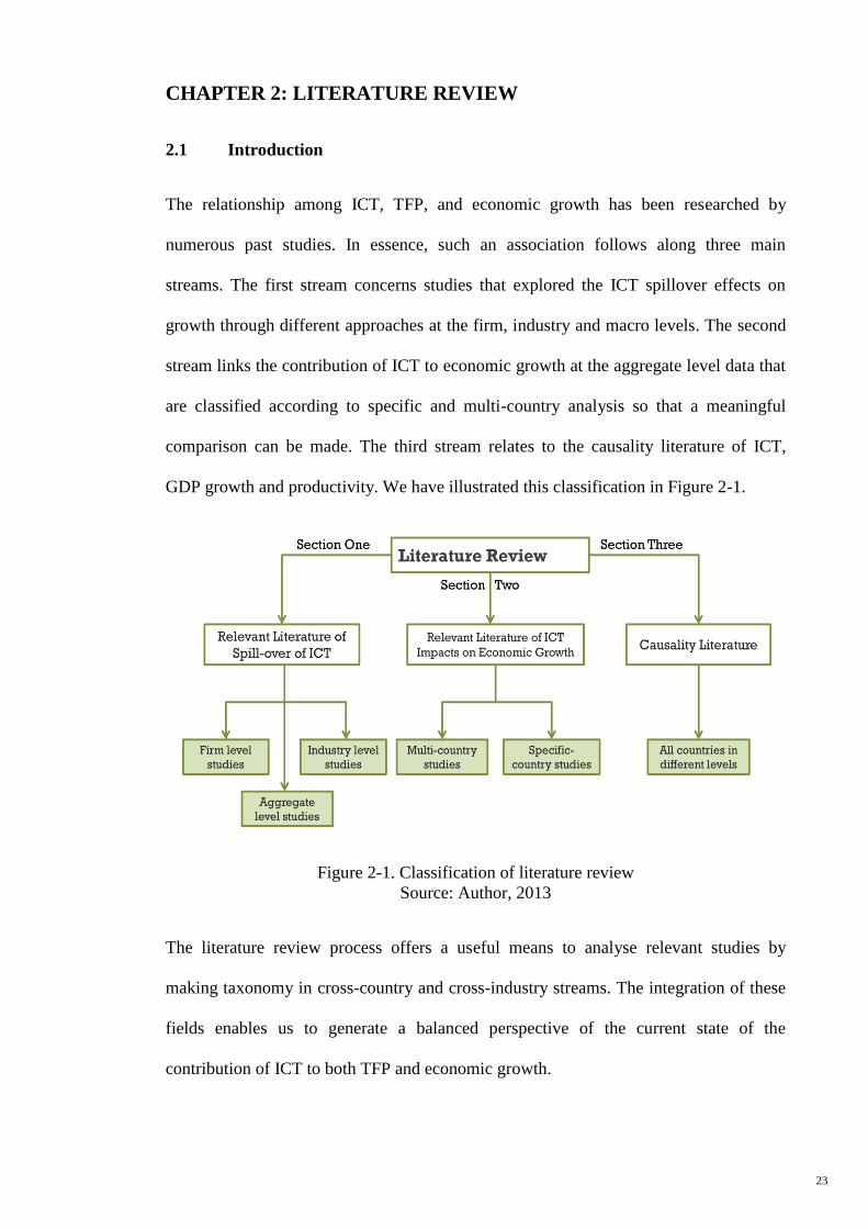
2.1 Introduction

The relationship among ICT, TFP, and economic growth has been researched by

numerous past studies. In essence, such an association follows along three main

streams. The first stream concerns studies that explored the ICT spillover effects on

growth through different approaches at the firm, industry and macro levels. The second

stream links the contribution of ICT to economic growth at the aggregate level data that

are classified according to specific and multi-country analysis so that a meaningful

comparison can be made. The third stream relates to the causality literature of ICT,

GDP growth and productivity. We have illustrated this classification in Figure 2-1.

Figure 2-1. Classification of literature review

Source: Author, 2013

The literature review process offers a useful means to analyse relevant studies by

making taxonomy in cross-country and cross-industry streams. The integration of these

fields enables us to generate a balanced perspective of the current state of the

contribution of ICT to both TFP and economic growth.

24

2.2 Relevant Literature concerning the Spillover of ICT at the Firm, Industry

and aggregate Levels

‘Spillover’ refers to the economic impact of ICT investment. By definition, it is an

increase in social welfare without compensation to the investors (Gholami, 2006).

According to ‘endogenous growth models’, innovation is a medium for technological

spillovers that enables less developed countries to catch up with the well-developed

ones. On the other hand, ICT capital seems to be characterised by forms of capital,

traditional forms of capital as a production technology and knowledge capital in its

informational nature (Dedrick, Gurbaxani, & Kraemer, 2003).

One key argument over the existence of the spillover of ICT is whether its capital stock

may also enhance economic growth towards TFP, particularly if the capital resembles

knowledge capital. The resources for economic growth may be relatively different over

time and across countries. However, innovation and technological changes have been

mainly approved as the determinants of growth. In addition, ICT has been considered as

the main form of technological transformation in recent decades (Madden & Savage,

2000). Dedrick et al. (2003) identified the ICT spillover effects as an opportunity for

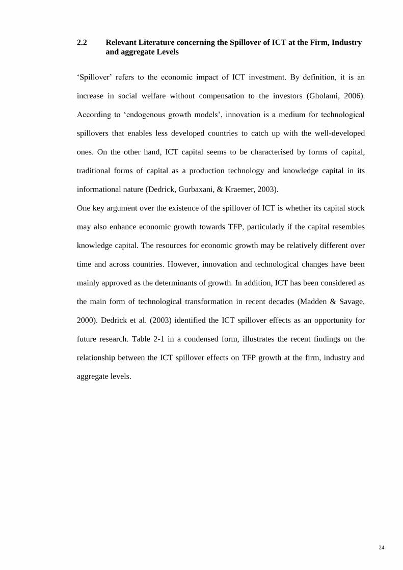
future research. Table 2-1 in a condensed form, illustrates the recent findings on the

relationship between the ICT spillover effects on TFP growth at the firm, industry and

aggregate levels.

25

Table 2-1. Summary of empirical studies on ICT spillover effects on TFP at the firm,

industry and national levels

Authors Period Case Study Method

Firm Level Studies

Arvanitis (2004) 1990-1993 Switzerland Labour productivity regressions

Atrostic et al. (2004) 2000 Denmark,

Japan, US Labour productivity regressions

Gretton et al. (2004) 1998 Australia Labour productivity regressions

Motohashi (2003) 1999 Japan Production function, TFP

Mariela Badescua (2009) 1994-1998 Spain Cobb-Douglass PF

Maliranta et al. (2008) 2008 Finland Production Function

Industry Level Studies Period Case Study Method Hans-Jürgen Engelbrecht

(2006) 1988-2003 New Zealand GLS

a

Diego Martínez (2010) 1980-2004 US Cobb-Douglass PF

Dimelis & Papaioannou(2011) 1990-2000 US, EU GMMb, panel data

Dahl et al.( 2011) 1970-2004 Japan, EU-US GMMb

Stiroh (2002) 1948-1999 US Growth accounting

Dedric et al. (2003) ------ More than 50

research papers

A Critical Review of the

Empirical Evidence

Michael J. Harper (2010) 1987-2006 US Growth accounting

Fueki & Kawamoto (2009) 1975-2005 Japan Growth accounting

Engelbrecht & Xayavong (2006) 1988-2003 New Zealand Difference-In-Difference

Regression

Mc Morrow et al. (2010) 1980-2004 US, EU ECMc

Kretschmer (2012) ------- OECD

countries

Review of on dynamic,

macroeconomic effects of ICT

Aggregate Level Studies Period Case Study Method Ketteni et al. (2007) 1980-2004 OECD Nonparametric techniques

Hwan-Joo & Young Soo (2006) 1992-1996 38 countries GLS

Elsadig Musa Ahmed (2008) 1960-2003 Malaysia Parametric model

Jalava (2003) 1975-2001 Finland Growth accounting

Jalava & Pohjola ( 2002) 1974-1999 US, G7 Comparison study

Jalava & Pohjola (2007) 1995-2005 Finland Production function

Christopher Gust (2004) 1992-1999 Industrial

countries Pooled regression estimates

Esteban-Pretel & Nakajima

(2010) 1980-1990 Japan Neo-classical growth

Dahl et al (2011) 1970-2004 Japan, EU-US GMMb

Bloom, Sadun et al. (2007,

2012) 1995-2003 US

Micro panel datasets, production

function

Antonelli & Quatraro (2010) 1970-2003 12 major

OECDs

Growth accounting, Cobb-

Douglas PF

Note: a

GLS: generalized least squares model, b GMM: generalized methods of moments approach,

cECM: Error Correction Mechanism specification


2.2.1 Firm level studies

As opposed to the aggregate and sectorial level analysis of ICT’s economic impacts,

firm level analysis is characterised by an extensive variety of methods and data. This is

partially due to the basic differences among the data. In fact, it also implies that an

extensive variety of approaches can be applicable to firm level data. Such diversity of

26

empirical evidence, being derived from different methods is considered stronger. This is

unlike cross-country comparisons, where there is a requirement for comparable data and

common methods.

According to the recent firm level studies, it was found that firm performance could be

impacted positively through the use of ICT. However, to a certain extent, the results

vary. Among the most notable results was that ICT-using the productivity performance

of the firm tended to be much better. In particular, the labour productivity of those firms

using one or more types of ICT was much higher than the firms that did not use ICT.

Furthermore, between 1997 and 1998 there was an increase in the gap between the firms

that used technology and the ones that did not, as there was an increase in the relative

productivity of firms using technology as compared to non-users (Pilat, 2004).

Australia is the fourth ranked ICT-developed country in the Asia Pacific region in which

technology has already had a significant impact (Gretton, Gali, & Parham, 2002). In

particular, Gretton, Gali and Parham (2002) found that both aggregation of firm level

and aggregate growth accounting have resulted in ICT, together with its related impact,

raising Australia’s TFP growth by approximately 0.2 per cent. Most significantly, the

econometric analysis at the firm level, which is controlling other impressive factors,

established positive links between productivity growth and ICT use for all the industrial

sectors examined. The results found in Australia have been confirmed by many studies,

such as Arvanitis and Loukis (2009) in Swiss and Jovanovic and Rousseau (2005) in

Finland, among others. Correspondingly, they found that productivity is closely

correlated to ICT use.

Badescua and Garcés-Ayerbe (2009) carried out a survey on Spanish firms where they

investigated the impact of IT on the productivity of labour using firm level

representative panel data. The survey involved 341 medium and large-sized firms. They

27

specifically employed the Cobb-Douglas production function to quantify the

contribution of information technology capital to labour productivity. Significantly, the

findings not only related to firm-specific, but corrected period-specific effects as well.

One explanation for this is that judging from the fact that ICT’s positive effects only

emerge after a long time, there is a huge lag between the education process and the

performance of new technologies.

A similar study in Finland (Maliranta, Rouvinen, & Airaksinen, 2008) involved

controlled time and industry effects. In particular, the researchers found that the impact

of ICT on the range of labour productivity, from 8 per cent to 18 per cent, corresponds

to 5 to 6 per cent elasticity of ICT capital. The effect is more pronounced in ICT-

producing services and new firms. With reference to this point, a study was conducted

by Atrostic et al. (2004) to examine the effect of computer networks in Japan, the

United States and Denmark (three OECD countries). Particularly, in Japan, it was

concluded that the usage of both inter-firm and intra-firm networks at the firm level was

positively correlated to the TFP levels. This is in line with the findings of Motohashi

(2003). In particular, Motohashi (2003) confirmed the establishment of a positive

coefficient for several types of network, including Electronic Data Interchange (EDI)

and open networks (Internet).

To sum up, the studies at the firm level discussed above demonstrated that productivity

is significantly improved by ICT, as is evident from its economic impact, but that it is

by no means a simple task to essentially convert the investment done in ICT into greater

productivity. Normally, changes in complementary investments, such as firm age and

size, organisational change, innovation and human capital are also required. It has

already been suggested in the discussion above that the effect of ICT may be greater

than the direct return effects flowing to firms that are ICT-producing and ICT-using

(Pilat, 2004).

28

2.2.2 Industry level studies

The literature review of ICT contribution has shown that in contrast to aggregate level

studies, industry level studies have been more conclusive. Aggregate level studies have

suffered due to the limitations present in their analysis. For example, a positive

correlation was found between economic growth and ICT at the country level in the

Asia-Pacific region (Dedrick, Gurbaxani, & Kraemer, 2003). However, the researchers

did acknowledge the lack of conclusive proof regarding the causal relationship due to

the comprehensive range of factors that affect economic growth, and also because the

economic allocation to ICT is relatively small in the overall capital.

To this point, it has been concluded that the use of ICT in portions of the services sector

is more widespread than in manufacturing albeit the same technology is not used by all

the sectors. Financial services is considered to be among the most ICT-intensive sectors

in many countries (Kretschmer, 2012). Among the OECD countries, the financial

intermediation sector was found to be the most likely sector to use network technologies

(OECD, 2003), which is an indication that this sector most probably profits from ICT

and that it is a considerable consumer of information.

There is a lack of evidence supporting the argument that the services sector has seen

strong performance growth due to the use of ICT at the industry level with the United

States and Australia being the exceptions (Kretschmer, 2012). In some cases, it has been

observed that the performance of the service sector can be enhanced by the use of ICT

at the firm level, more so in countries where there is slight proof of accessibility at the

industry level. As for the case of the United States and Australia, the industry level

evidence was confirmed by studies conducted at the firm level (Gretton, Gali, &

Parham, 2004). Maliranta and Rouvinen (2008), and Arvanitis (2009) in Finland and

Switzerland proved that in the manufacturing sector the Internet does not play an

important role in terms of performance as compared to the service sector. This is

29

probably due to the lack of desk job work, personal computers and Internet connections

for the manufacturing workers.

Atrostic et al. (2004) used the Badescua and Garcés-Ayerbe (2009) method for New

Zealand at the industry level but that they did not obtain similar results, which proves

that the results are sensitive to the time period specified. Engelbrecht and Xayavong

(2006) used the breaking period of the study approach sub-periods over 1988-2003 to

support that labour productivity growth of ICT intensive industries has improved more

than for other industries, albeit the overall labour productivity growth was weak.

The dynamic general equilibrium approach on US industries revealed the same as New

Zealand's results, which have shown the sensitivity of productivity growth from ICT on

the time specification (Engelbrecht & Xayavong, 2006; Martínez, Rodríguez, & Torres,

2010). As a result of the interpretation, it can be concluded that there is a large gap

between the learning and running operation of new technologies, which indicates that its

positive impact on the firms emerges after a moderately long period of time. In 2002,

the Federal Reserve Bank of the US published a surprising result from a broad survey

about the effect of TFP and labour productivity (APL) growth on the ICT- producing

sectros in the US manufacturing industries. The results of this comprehensive research

revealed that the neoclassical framework identified five different input measurement

errors, i.e. omitted variable, increasing return, reserve causality, production spillover

and network externalities, that have an existing correlation between ICT and TFP

growth. The data collection for TFP was first completed by the Bureau of Labour

Statistics (BLS) in the United States and then APL and TFP6 were estimated by using

equations (2.1) and (2.2) (z: proxy) for the two main digital manufacturing industries.

(2.1)

dLn APL = dLn Y- dLn H APL growth

6TFP growth is defined as output per all inputs, and ALP growth is output per hours worked. See the discussion of productivity in

the July 2001 issue of Business Economics for details.

30

(2.2)

dLnZ = dLnY-αk Ln K-αH Ln H-αM Ln M TFP growth

Where Y is output growth, H is human resources, K and M, non-ICT and ICT capitals.

Therefore, the dLnZ is measured as a residual to fulfil the equality. This model is

estimated in the neoclassical model based on Solow's (1987) and Jorgenson's (1987)

assumptions of the growth model (Stiroh, 2002a, 2002b).

Other scholars extended Stiroh’s approach by adding more observations; Harper,

Khandrika, Kinoshita, and Rosenthal (2010) for the US industries, and Fueki and

Kawamoto (2009) for the Japanese industries, which have addressed negative

coefficients for ICT as a non-impressive factor. In contrast with Sitroh’s (2002a) results,

another research established the contribution of ICT-specific technological changes in

productivity growth that was about 0.73 per cent, while non-ICT capital assets were

only 0.16 per cent. It is noteworthy to mention that the contribution of ICT has

increased from the mid-1990s while the contribution of non-ICT capital inputs has

decreased (Martínez et al., 2010). For a better understanding of this surprising result,

Stiroh (2002b) decomposed ICT into computers and telecommunications equipment and

then estimated them again. The findings revealed the existence of considerable

differences between the two types of equipment of ICT and heterogeneity in

productivity shock across industries.

Identifying the determinants of the TFP growth gap using industrial level data for the

US and EU using the panel data approach was carried out by McMorrow, Röger, and

Turrini (2010), and Dimelis and Papaioannou (2011). In the previous studies, TFP

growth was significantly fuelled by developments at the "technological frontier" since

the 1990s for both the US and the EU. Moreover, TFP growth in the US was stronger

than the EU at the end of the 1990s due to more Research and Development (R&D)

31

expenditure and upper adoption rates for ICT intensive technologies. Mc Morrow et al.

(2010), employing Least Squares Dummy Variables (LSDV), and Dimelis &

Papaioannou (2011), using Pooled Mean Group (PMG) and Generalised Moment of

Method (GMM) estimators, claimed that the ICT impact on productivity was primarily

exhibited in the industries that were either heavy ICT users or producers and stronger

network utilities. Recent efforts were made by the EU zone to investigate the connection

between TFP growth and ICT in cross-industry and cross-country simultaneously (Dahl,

Kongsted, & Sørensen, 2011). To sum up, the results of the EU and the US studies

arrived at a common conclusion that due to ICT’s slow adoption in the EU industries,

the EU has limited acceleration of productivity and economic growth. Comparatively,

the US has seen its productivity grow faster than the EU because the ICT-producing

sector had a larger employment share and the rapid productivity growth of the services

industries extensively utilised ICT.

Cross-industry studies regarding the ICT’s productivity or spillover effects are

relatively quite rare, mainly due to comparable data sources being fairly new. To sum

up, the results for the industrial level are more concerned with the US due to the slow

adoption of ICT in the EU industries. Furthermore, industries that produce or use ICT

most intensively have shown the largest increases in productivity growth after 1995

(Stiroh, 2002a, 2002b). Nevertheless, there is little evidence that rapid TFP growth has

been experienced by ICT-using industries, with the major exceptions being Australia

and the United States (Pilat, 2004).

2.2.3 Aggregate level

Difficult questions are raised when the role of ICT is examined at the firm, sectoral and

aggregate levels, which we are trying to address by classification of the literature

according to the firm, industry and aggregate levels. There is little evidence that at the

32

industrial level more total factor productivity growth has been experienced by ICT-

using, with the major exception being Australia and the United States (Pilat, 2004).

The wedge among the impacts observed at the macroeconomic level and those for

industrial and individual firms, which could be created by the spillover effects, may not

yet have been beneficial for some European countries. It has been argued that the

impact of direct returns flowing to the ICT-using industries and firms may be less than

the impact of ICT. For instance, there could be an improvement in the functioning of the

markets (through the process of improved matching) and there is a possibility of making

new markets, which could be due to the lower transaction costs of ICT. The impact of

ICT on innovation and knowledge creation is another effect that could potentially create

a gap between the aggregate returns and firm-industry level returns. The process of

knowledge creation could be increased through the use of ICT, as it facilitates the

processing of data and information at a greater speed. These kinds of spillover effects

may have already been highlighted in the United States aggregate statistics, but this is

not the case in other countries thus far.

Moreover, the impact of ICT in aggregate and sectoral analysis might be disguised due

to the effects on economic changes and the aggregation across industries and firms. This

is also due to the dependence of the impacts of ICT on policy changes and other factors,

which might vary across industries. The scope of the aggregate effects over a period of

time is dependent on the rate at which ICT develops their lags, diffusion, adjustment

costs, complementary changes and ICT’s potential of productivity-enhancement in

diverse industries (Gretton, Gali, & Parham, 2004). It is by no means a straightforward

task to disentangle such factors at the industry or aggregate level.

Concerning the evolution of TFP for 38 countries, Hwan-Joo and Young (2006)

suggested that the digital divide, on the one hand, widens the growth gap among

countries, which is the negative impact of ICT-using. On the other hand, the global ICT

33

diffusion generates ICT externalities, which have a positive effect on the total factor

productivity of less-developed countries.

The results for Malaysia, as an Asian economy, revealed that the increasing knowledge

of the labour factor has a significant effect on the performance of TFP in respect of

economic growth (Elsadig, 2008). The impacts of ICT and human capital on Malaysia’s

productivity growth have been highlighted and the results have been adopted by

policymakers. The log-linear based model is used, which measures the elasticity of

variables, the autoregressive regressor estimated labour productivity factor (APL)

growth into contribution of capital deepening (K/L), increasing ICT usage (ICT/L),

human capital intensity and TFP per unit labour growth between 1960 and 2003. The

findings of Elsadig (2008) for Malaysia support the study of Martínez et al. (2010) that

APL significantly influences capital deepening. In contrast with the linear relationship

between these variables, Ketteni, Mamuneas, and Stengos (2007) also proved the

existence of a nonlinear relationship between the mentioned variables by using

nonparametric techniques for members of OECD during 1980-2004.

Based on the results obtained in Finland and the US, which are considered leaders in

information societies with respect to Nokia’s revolution in the telecommunication

industry Finland has demonstrated that the contribution of ICT is 1.87 per cent of the

monitored labour productivity growth. Despite the fast growth of TFP in the ICT-

producing industries, it has had an even larger impact on Finland; however, in the US,

there has been no evidence of any significant acceleration in the rate of labour

productivity (Jalava, 2003; Jalava & Pohjola, 2002, 2007).

However, Jalava and Pohjola (2007) argued that ICT could increase the economic

growth via the spillover effects of ICT through to TFP. In the suggested model, the

aggregate input consisting of ICT capital services (KICT), other capital services (KO),

and labour services (L) produced total outputs under equation (2.3).

34

(2.3)

Y (YICT (t), Y0 (t)) = A (t) F (k ICT (t), k0(t), L(t))

It is of interest to compare the European evidence to the US results in this research. In

this respect, four other related papers by Gust and Marquez (2004), Pilat (2004),

Esteban-Pretel, Nakajima, and Tanaka (2010), and Dahl et al. (2011), captured the

general consensus about productivity growth performance in the EU economies that was

mostly described by an unpromising performance of the ICT-using industries. These

studies provided evidence, especially for high, middle income, European countries and

the US. They created a perspective that can be used to measure productivity divergence

between European industrial countries and the United States by stressing the role of

managing practices in influencing the diffusion of ICT.

According to the above studies, ICT has a positive effect on productivity growth in

Europe; nonetheless, the effects found for the US are more than twice the effects found

for Europe. To some extent, the divergence in productivity levels between the two

regions is due to the difference in the utilisation of ICT; however, the decline in the

European productivity growth after 1995 is not explained by this. Regardless of the

positive effects that ICT has on productivity growth, European productivity growth is

still declining. Therefore, there was a decrease in Europe’s aggregate and industry

averages of productivity growth after 1995. One reason as to why there was greater

growth performance of ICT in the US economy to that of non-US countries was put

forward by Bloom, Sadun, and Reenen (2007, 2012), and Pilat (2004). The authors

presented evidence pointing towards the US management style practices that relate to

ICT being used more productively.

They mentioned an unresolved and a very important issue concerning where study on

the effects of ICT on TFP growth was done using two different approaches and which

generated different results. Significant and positive effects were found for TFP growth

35

when production functions were estimated post-1995. In contrast, some of the results

have applied a traditional growth accounting background that shows no significant

productivity growth acceleration in Europe and OCED countries because of the delay in

technology adoption compared to the US. Both approaches apply different restrictions,

which may be the likely cause of the difference found (Antonelli & Quatraro, 2010).

Another suggested reason for this divergence is that the success of the countries in

implementing ICT may be down to the ability to gain market share and growth in

competitive markets, the United States as compared to less competitive markets.

Consequently, there would be a greater contribution to the overall impact of ICT in the

US. Moreover, there is an active role of competition in determining the effect size of the

spillover. In a competitive market, which is quite large and highly intensive, as in the

United States, the largest beneficiaries of investment in ICT may not be the firms using

ICT but the effect on the aggregate performance of the country (Pilat, 2004).

Finally, the most important reason for this difference can be due to the measurement

playing a role. In most countries, sectoral and macroeconomic data may be insufficient

to identify the impact of ICT due to the different ways output is measured. For instance,

the convenience brought about by the introduction of automated teller machines has led

a few countries to change the way banking output is measured, as in the United States.

As the primary user of ICT is the services sector, it would be a considerable problem if

there is a difficulty in measuring service output.

In conclusion to this part of the literature, the most widely used approach to estimate the

spillover effects of ICT have been industry or firm level data usage. The comparison

between the results obtained from the studies done on European countries and the

United States is particularly interesting. According to the above, there is a positive

spillover effect of ICT on productivity growth in Europe; nonetheless, the effects found

in the US are more than twice that of Europe. As a justification to this profound

36

difference, many reasons have been suggested by previous studies. It is interesting to

investigate Asia-Pacific countries, which are leaders in ICT development and also

followed the EU productivity paradox after 1995. Furthermore, the presented discussion

showed that aggregate evidence might lead to an apparent productivity paradox in the

EU whereas there is little evidence of the paradox for the industry and firm level data

used.

2.3 Relevant Literature concerning the impact of ICT on Economic Growth

Recent theories concerning economic growth predict that economic growth depends on

investment in ICT. Nevertheless, empirical studies have suggested combined results

based on the region, the time period and the type of industry considered. Moreover,

some surveys support that the growth gap between the developed countries and

underdeveloped countries is associated with the ICT diffusion and the productivity and

growth rate of those countries. This part of the literature has been surveyed under two

processes, namely, multi-country literature surveys and specific individual countries.

2.3.1 Multi-country studies on ICT – economic growth nexus

Table 2-2 presents the chronological list of empirical works conducted on the

association between ICT contribution and economic growth based on authors, time

frame, country, and methodology in multi-country and specific-country streams.

In a joint study, Hosseini Nasab and Aghaei (2009) considered the economy of OPEC

member countries between 1990 and 2007. The long run growth of the economy with

the neoclassical model of capital accumulation, as well as using the dynamic panel data

framework and employing a Generalized Method of Moments (GMM), found a

significant impact of ICT investment on economic growth (Mankiw, Romer, & Weil,

1992).

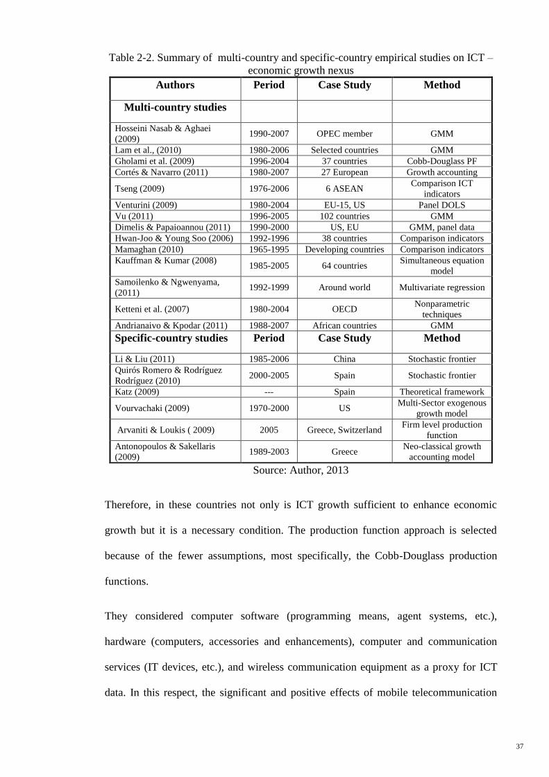
37

Table 2-2. Summary of multi-country and specific-country empirical studies on ICT –

economic growth nexus

Authors Period Case Study Method

Multi-country studies

Hosseini Nasab & Aghaei

(2009) 1990-2007 OPEC member GMM

Lam et al., (2010) 1980-2006 Selected countries GMM

Gholami et al. (2009) 1996-2004 37 countries Cobb-Douglass PF

Cortés & Navarro (2011) 1980-2007 27 European Growth accounting

Tseng (2009) 1976-2006 6 ASEAN Comparison ICT

indicators

Venturini (2009) 1980-2004 EU-15, US Panel DOLS

Vu (2011) 1996-2005 102 countries GMM

Dimelis & Papaioannou (2011) 1990-2000 US, EU GMM, panel data

Hwan-Joo & Young Soo (2006) 1992-1996 38 countries Comparison indicators Mamaghan (2010) 1965-1995 Developing countries Comparison indicators Kauffman & Kumar (2008)

1985-2005 64 countries

Simultaneous equation

model

Samoilenko & Ngwenyama,

(2011) 1992-1999 Around world Multivariate regression

Ketteni et al. (2007) 1980-2004 OECD Nonparametric

techniques

Andrianaivo & Kpodar (2011) 1988-2007 African countries GMM

Specific-country studies Period Case Study Method

Li & Liu (2011) 1985-2006 China Stochastic frontier

Quirós Romero & Rodríguez

Rodríguez (2010) 2000-2005 Spain Stochastic frontier

Katz (2009) --- Spain Theoretical framework

Vourvachaki (2009) 1970-2000 US Multi-Sector exogenous

growth model

Arvaniti & Loukis ( 2009) 2005 Greece, Switzerland Firm level production

function

Antonopoulos & Sakellaris

(2009) 1989-2003 Greece

Neo-classical growth

accounting model


Therefore, in these countries not only is ICT growth sufficient to enhance economic

growth but it is a necessary condition. The production function approach is selected

because of the fewer assumptions, most specifically, the Cobb-Douglass production

functions.

They considered computer software (programming means, agent systems, etc.),

hardware (computers, accessories and enhancements), computer and communication

services (IT devices, etc.), and wireless communication equipment as a proxy for ICT

data. In this respect, the significant and positive effects of mobile telecommunication

38

development on economic growth conducted by Lam et al. (2010) supported the above

discussion in high-income countries while Gholami et al. (2006) asserted that

developing countries could gain more than industrialised or developed countries

through the employment of ICT.

One of the empirical studies on the impact of ICT on growth in the group of countries

that were using industry level data was conducted by Dimelis & Papaioannou (2011)

who researched over two sub-periods, i.e. 1980-1990 and 1990-2000 for the US and EU

industries. Normally, factors related to novelty activity, employment of highly skilled

human capital, and Research and Development (R&D) lead to TFP growth. Increased

investment in information and communication technology (ICT) capital and growth in

human capital contributed substantially to labour productivity growth in market services

across all European countries and the US (Inklaar, Timmer, & Van Ark, 2008). In

accordance with these results, Cortés and Navarro (2011) believed that countries differ

most strongly in the rates of efficiency improvement in the use of inputs and different

ICT diffusion. Hence, it was debated as to whether they have also captured different

levels of human development (Cortés & Navarro, 2011). A similar story was proven in

the newly industrialized Asian countries, such as South Korea, Taiwan, Singapore,

Hong Kong, China and India, which have enjoyed a large contribution of ICT in

economic growth through four main knowledge and innovation network indices in ICT

(Tseng, 2009).

In 15 EU countries and the US, industrial growth has been captured by using log-linear

transformation of the Cobb-Douglass production function with respect to TFP, labour,

non-ICT and ICT as factors of production. The long run elasticity of ICT is captured by

running Panel Dynamic OLS (PDOLS) and panel cointegration analysis (Venturini,

2009). Based on the same results as above, Ketteni et al. (2007) concluded that these

39

are run on a nonlinear approach among ICT capital, human capital, initial income, and

economic growth.

In this sense, Vu (2011), Andrianaivo and Kpodar (2011) overcame the endogeneity

issues by applying System GMM estimators that exhibited that the growth behaviour of

ICT was not similar across the time period at a global level. Therefore, there are

distinctions in ICT growth impacts in the ICT-using and ICT-producing sectors over the

mentioned period, especially when the ICT effects significantly increased during the

1990s in both the US and EU countries. In this regard, Dimelis and Papaioannou, (2011)

compared the long run relationship results between using PMG and GMM estimators.

Part of the positive impact of mobile phone penetration on growth for African countries

came from superior financial inclusion.

One distinctive study revealed that non-ICT investment has a cumulative causal

relationship with economic growth that played a key role in the process of widening the

growth gap. ICT investment did not have a strong interdependent relationship with

economic growth across 29 countries in the 1990s. This paper introduced a new

measurement for the gap in growth using simultaneous equation, three-stage least

squares (3SLS) and classifying two groups of countries – frontier group and follower

group countries. According to equation (2.4), the growth gap defined the discrepancy of

productivity in the two groups (Hwan-Joo, Young, & Jeong, 2009).

(2.4)

Gi=Ln

Where Gi is the growth gap between two groups, which are frontier group and follower

group countries, PROF and PROI are productivity in frontier group and follower group

countries, respectively. Equations (2.5) and (2.6) showed that the output and

40

productivity functions for the two groups of countries have been driven by the average

total product:

(2.5)

Yi = AiLiα

NICTiβICTi

γ

(2.6)

PRO i =

=

α β γ

Where, Yi is output, L, NICT, ICT as labour non-ICT and ICT inputs, and PROi labour

productivity. In spite of the main variables like ICT and non-ICT, many explanatory

variables like degree of openness to trade, ratio of high-technology exports, and

secondary education have been employed, therefore, the unbalanced panel data is

suggested in four simultaneous equations (Hwan-Joo & Young, 2006).

Mamaghani (2010), in support of Weber and Kauffman (2011), analysed social,

economic and other components that drive global ICT adoption and the organisational,

individual, industrial, and economic impacts. This has raised efforts to use ICT to attain

a variety of spillover development effects with poverty declining, expansion of health

services, extension of educational opportunities and access to government services. In

contrast with Mamaghani (2010), Weber and Kauffman (2011), Samoilenko and

Ngwenyama (2011) have jointly pointed out that the insignificant impact of the ICT

investments on the economics have been due to a shortage of technologically skilled

ICT workers who could not adapt themselves to the new circumstance of using ICT.

2.3.2 Specific-country studies on ICT– economic growth nexus

In general, researchers have transmitted the effect of ICT on economic growth through

three channels. Firstly, ICT is involved as an output or direct contribution to the

41

production of ICT7 from total value added. Secondly, the ICT capital factor provides

economic growth as an input factor in production function. Finally, ICT can increase the

economic growth via the ICT-production effects on total factor productivity. This

section analyses and summarises the recent studies using a second approach in each

individual country and its comparison with non-ICT impacts, which, occasionally, are

in conflict across different countries.

A translog production with stochastic frontier model for Chinese and Spanish

manufacturing firms estimated the economic growth with respect to human capital and

the efficiency of technology for China and Spain (Romero & Rodríguez, 2010). The

behaviour of Spanish firms has justified that the e-buying process had a positive impact

on firm efficiency, but it became insignificant in the case of e-selling, unlike for the

Chinese firms. The empirical results show an improvement in technical progress and its

efficiency as the major contributor of the productivity growth but that input growth is

the main contributor to GDP growth in the provinces of China (Li & Liu, 2011).

The indirect effects of ICT on US and Spanish economies have been researched by Katz

(2009) and Vourvachaki (2009). Multi-sector frameworks that rely on consumer

behaviour proved that even the non-ICT-using sector of the US benefited indirectly

from ICT, while households' utility increases through using ICT services. However,

they proved that if TFP growth and employment establishment were driven partially by

the level of ICT investment and telecommunications in the Spanish sector, a reduction

in capital expenditure as a result of a certain regulatory framework would have an

important effect on the economy.

A comparative study on Greece and Switzerland concerning their production function

framework at the firm level revealed that Swiss firms are more mature and efficient than

7The approach in this paper is different from Jorgenson et al. (2003) in that they only include ICT investment goods in the

production of ICT.

42

Greek firms in using and creating novelty in ICT as an input (Arvanitis & Loukis,

2009). At the same time, another comparative study between Greece and the US

conducted by Antonopoulos and Sakellari (2009), at the industrial level, manifested that

ICT investment led to a resurgence of economic resources and TFP growth in Greece.

Especially, Arvanitis and Loukis (2009) stated that business services, insurance,

finance, wholesale and retail trade industries were the sectors that benefitted most.

Unlike the US government and firms, Spain and Greece underrated the benefits of ICT

investment, even some of Germany's key sectors had problems in fully exploiting the

benefits of ICT. This is because Germany seems to suffer from underinvestment in both

IT and software (Welfens, 2008).

In conclusion of this section, we have determined that evidence in multi-country

literature studies addressed more comparative studies in the EU and US. Nevertheless,

they did not cover the ICT development status of countries to investigate the existence

of a relationship between the rank of ICT development and its positive effect on

economic growth. The majority of the studies only considered the income level of

countries to configure comparative studies and paid little attention to the ICT position of

countries. We will follow the multi-country studies in Asia-Pacific and European

countries as two different regions. We will cover this gap with our findings in 12 Asia-

Pacific and European countries, which are leaders in ICT development in the two

regions. We will obtain from our findings whether divergence in economic growth

among different countries is due to increasing ICT contribution in the mentioned

regions.

2.4 Causality Literature

Although a significant growth in the use of ICT was stated to be an important factor

affecting economic growth, its contribution has differed from one country to another

43

and at different developmental stages. Causality tests to assess the causal relationship

between economic growth and development of telecommunications were investigated

by Hardy (1980); Cronin, Parker, Colleran and Gold (1991); Cronin, Colleran, Herbert

and Lewitzky (1993), and Madden and Savage (1998). They found bidirectional

causation between infrastructural telecommunication and economic growth in the

United States and Central and Eastern European (CEE) countries.

The effect of investment in telecommunication infrastructure on the GDP in 21 OECD

countries and emerging industrialized non-OECD countries from 1970 to 1990 was

studied by Röller and Waverman (2001). They also reported that the effect is not linear,

and that it is higher in OECD countries compared to non-OECD countries. The analysis

carried out by Dutta (2001) on 15 industrialized and emerging economies showed that

the causality from telecommunication infrastructure to economic activity was stronger

compared to the reverse. Datta and Mbarika (2006) found evidence of causality running

from information technology development to the growth of service sectors by extending

the dataset of Dutta (2001).

A bidirectional association was found between GDP and tele-density for the long and

short run in the 12 emerging economies in Asia by Chakraborty and Nandi (2003).

Separating the countries into two groups with a high and low level of privatization, the

causality was only bidirectional for the countries in the first group. For the low level of

privatization group, causality ran from tele-density to GDP in the long run. A positive

and significant causal association was found between the regional level of income and

ICT infrastructure in Poland, with causality running from the former to the latter

(Cieślik & Kaniewska, 2004). In South Korea and the US, a bidirectional association

was found between investments in information technology and economic growth

(Wolde, 2007).

44

Shiu and Lam (2007) observed a unidirectional relationship from GDP to

telecommunications development in China. However, the reverse causality was

observed in the affluent eastern region, not in the low-income central and western

provinces. Poor infrastructural telecommunication (i.e. tele-density unable to attain

“critical mass”) as well as the complementary factor of a low level of economic

development (education and training) are some of the reasons for the shortfall in the

income effects of the development of telecommunication in the low income western and

central provinces. These findings are consistent with previous research that found

limitations to the effect of ICT on the growth of the economy or on foreign direct

investment in the less developed economies (Dewan and Kraemer, 2000; Jalava and

Pohjola, 2002; Gholami, Sang-Yong, & Heshmati, 2006).

Roller and Waverman (1996, 2001), Karner and Onyeji (2007) demonstrated that the

impact of ICT on economic development was dependent on the level of growth of ICT.

In the advanced economies, as well as areas with high ICT growth, a bidirectional

association was found between the development of ICT and economic growth (Lam &

Shiu, 2010). In recent research on the General Purpose Technology (GPT) hypothesis,

Kretschmer (2012) found strong positive evidence of ICT and TFP growth for United

States data; however, it was more difficult to find such evidence in Europe. Therefore, it

has been suggested that investigating how spillovers work with ICT may bridge this

knowledge gap, particularly since many questions on the subject of possible

externalities remain unanswered.

In summary, based on our knowledge from this section, no more attempts have so far

been completed to examine the causal relationship between ICT and various

determinants of economic growth relying on the Pooled Mean Group (PMG) estimators

with the Vector Error Correction Model (VECM) framework on panel data analysis

methodologies. Therefore, we are targeting to test the presence and nature of any causal

45

relationship between GDP growth and the contribution of ICT, non-ICT, labour and

TFP in the long run and short run by using PMG estimators. Previous research has

hypothesized that the rich ICT infrastructure of the receiving host country may increase

TFP, which will indirectly lead to economic growth and catch up with the ICT effects

on TFP growth through the causality tests. The main contribution of this study is the

construction of a comprehensive analysis of causality among the primary key variables

of ICT on GDP growth in a multivariate framework in cross-country and cross-industry

panel data.

Moreover, this study allows explanation of the differences in the returns of ICT factors

separately in ICT-using and ICT-producing sectors across the Asia-Pacific and

European countries. The findings of this study will have two aspects of empirical

implications. Firstly, it will fill the gap in the literature concerning the causal

relationship between ICT and TFP and its impact on economic growth. Secondly, as

shown by the causality, it suggests that ICT infrastructure is a significant driver of

growth in the long run, henceforth, they should accelerate their ICT deployment.

2.5 Identification of Research Gap

According to the reviewed literature, we have identified the following research gaps that

have not been adequately addressed by previous scholars.

1. The review of the assumption of the growth accounting approach has manifested that

this framework is less able to fully capture the impact of ICT on economic growth

because it does not consider the spillover effects of the impact of ICT. An essential

feature of the existence of ICT spillover is whether the ICT capital stock may also boost

economic growth through positive spillover effects on TFP if ICT capital is like

knowledge capital. Moreover, a major shortcoming traditional growth accounting

46

suggested by Solow is that it does not cover a significant dimension of the technological

changes.

On the other hand, according to the ‘endogenous growth models,’ innovation is a

medium for technological spillover effects that permit less developed countries to catch

up highly developed countries. Moreover, ICT capital seems to have the characteristics

of both forms of capital – traditional forms of capital as a production technology and

knowledge capital in its informational nature (Dedrick, Gurbaxani, & Kraemer, 2003).

Therefore, we will peruse the ICT impacts from the neo-classical growth model due to

ICT as an input of production function and endogenous growth model to deal with ICT

spillover effects. Nevertheless, our results are believed to help in taking a modest step

towards a deeper perception of the role of ICT in total factor productivity and economic

growth.

2. Cross-industry studies on the growth impacts of ICT are still relatively limited,

mainly because comparable data sources are quite new. We employ the EU KLEMS

database as a unique source in order to be able to compare industrial level findings.

Moreover, our study allows explanation of the differences in return of ICT factor

separately in ICT-using and ICT-producing sectors across the Asia-Pacific and

European countries.

3. Based on the above studies, ICT has a positive effect on productivity growth in EU

countries; however, it is less than half of the dimension of the effect found in the US.

The present discussions will respond to questions concerning whether aggregate

evidence may lead to an apparent productivity paradox in Asia-Pacific and EU countries

whereas industry level data presents little evidence for a paradox. To justify this

difference, many reasons have been suggested by previous studies, but it is interesting

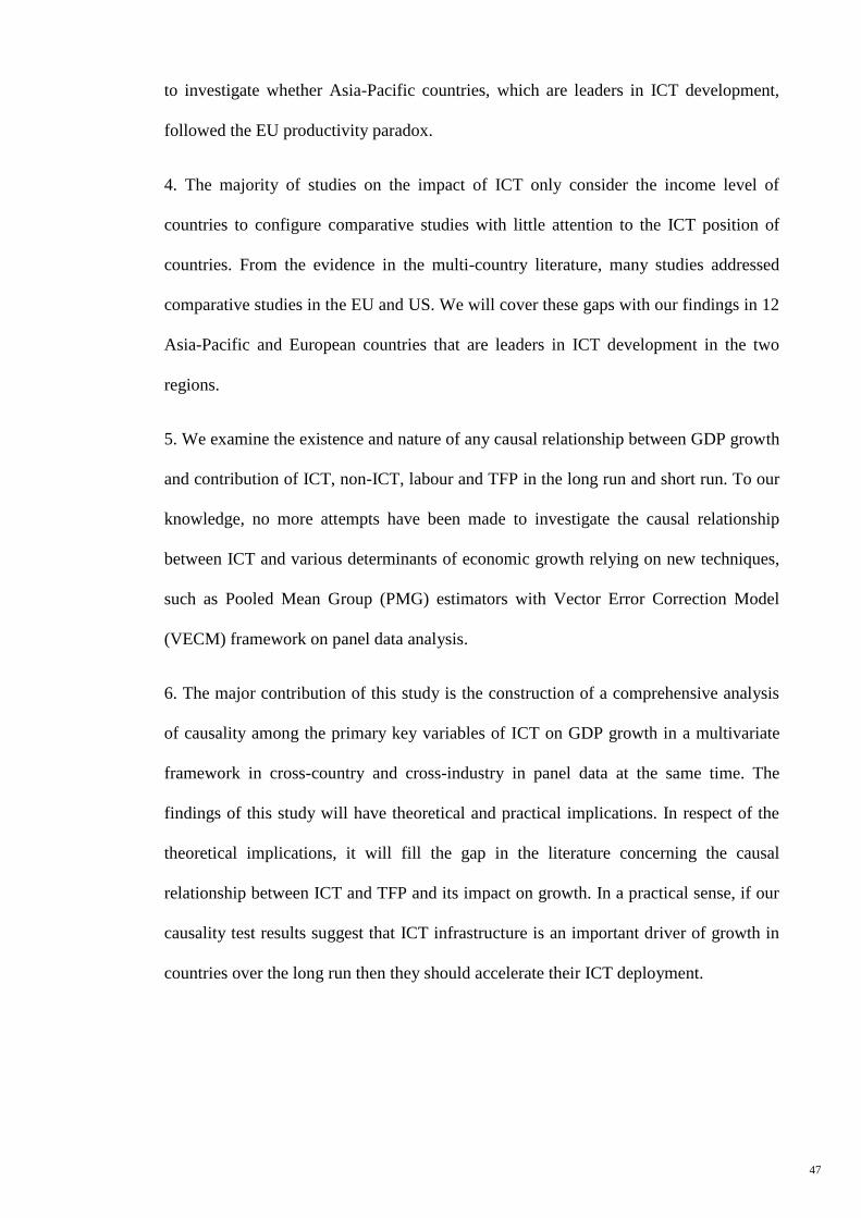
47

to investigate whether Asia-Pacific countries, which are leaders in ICT development,

followed the EU productivity paradox.

4. The majority of studies on the impact of ICT only consider the income level of

countries to configure comparative studies with little attention to the ICT position of

countries. From the evidence in the multi-country literature, many studies addressed

comparative studies in the EU and US. We will cover these gaps with our findings in 12

Asia-Pacific and European countries that are leaders in ICT development in the two

regions.

5. We examine the existence and nature of any causal relationship between GDP growth

and contribution of ICT, non-ICT, labour and TFP in the long run and short run. To our

knowledge, no more attempts have been made to investigate the causal relationship

between ICT and various determinants of economic growth relying on new techniques,

such as Pooled Mean Group (PMG) estimators with Vector Error Correction Model

(VECM) framework on panel data analysis.

6. The major contribution of this study is the construction of a comprehensive analysis

of causality among the primary key variables of ICT on GDP growth in a multivariate

framework in cross-country and cross-industry in panel data at the same time. The

findings of this study will have theoretical and practical implications. In respect of the

theoretical implications, it will fill the gap in the literature concerning the causal

relationship between ICT and TFP and its impact on growth. In a practical sense, if our

causality test results suggest that ICT infrastructure is an important driver of growth in

countries over the long run then they should accelerate their ICT deployment.

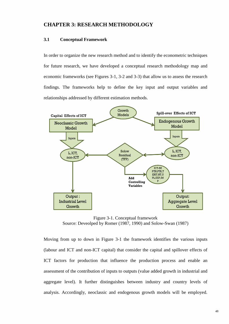
48

3 CHAPTER 3: RESEARCH METHODOLOGY

3.1 Conceptual Framework

In order to organize the new research method and to identify the econometric techniques

for future research, we have developed a conceptual research methodology map and

economic frameworks (see Figures 3-1, 3-2 and 3-3) that allow us to assess the research

findings. The frameworks help to define the key input and output variables and

relationships addressed by different estimation methods.

Figure 3-1. Conceptual framework

Source: Deveolped by Romer (1987, 1990) and Solow-Swan (1987)

Moving from up to down in Figure 3-1 the framework identifies the various inputs

(labour and ICT and non-ICT capital) that consider the capital and spillover effects of

ICT factors for production that influence the production process and enable an

assessment of the contribution of inputs to outputs (value added growth in industrial and

aggregate level). It further distinguishes between industry and country levels of

analysis. Accordingly, neoclassic and endogenous growth models will be employed.

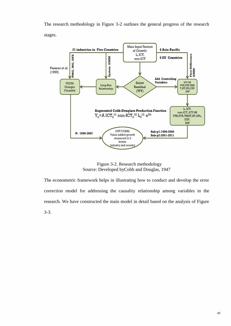
49

The research methodology in Figure 3-2 outlines the general progress of the research

stages.

Figure 3-2. Research methodology

Source: Developed byCobb and Douglas, 1947

The econometric framework helps in illustrating how to conduct and develop the error

correction model for addressing the causality relationship among variables in the

research. We have constructed the main model in detail based on the analysis of Figure

3-3.

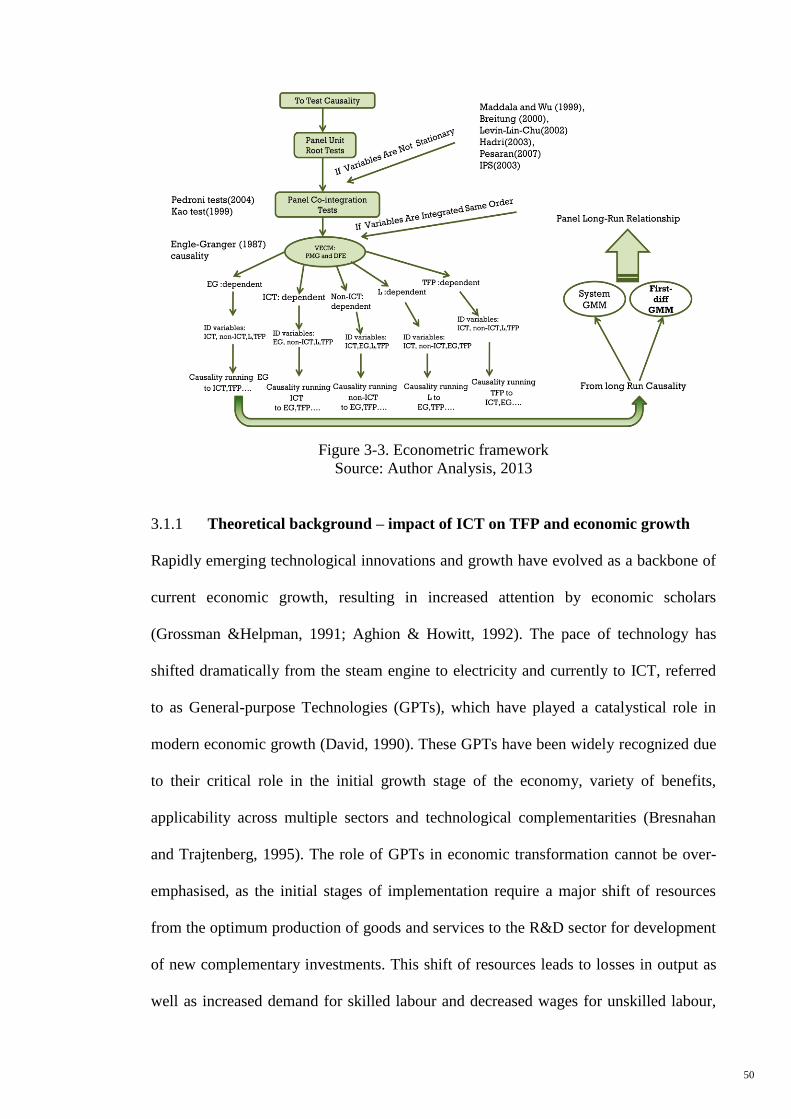
50

Figure 3-3. Econometric framework

Source: Author Analysis, 2013

3.1.1 Theoretical background – impact of ICT on TFP and economic growth

Rapidly emerging technological innovations and growth have evolved as a backbone of

current economic growth, resulting in increased attention by economic scholars

(Grossman &Helpman, 1991; Aghion & Howitt, 1992). The pace of technology has

shifted dramatically from the steam engine to electricity and currently to ICT, referred

to as General-purpose Technologies (GPTs), which have played a catalystical role in

modern economic growth (David, 1990). These GPTs have been widely recognized due

to their critical role in the initial growth stage of the economy, variety of benefits,

applicability across multiple sectors and technological complementarities (Bresnahan

and Trajtenberg, 1995). The role of GPTs in economic transformation cannot be over-

emphasised, as the initial stages of implementation require a major shift of resources

from the optimum production of goods and services to the R&D sector for development

of new complementary investments. This shift of resources leads to losses in output as

well as increased demand for skilled labour and decreased wages for unskilled labour,

51

thereby affecting the overall economy or Total Factor Productivity (TFP). Once the

economy has gone through this critical stage and complementary investments have been

developed successfully, the application of GPTs is realised across multiple sectors. The

national economic cycle enters into a new stage of accelerated TFP and output growth

along with a significant rise in the labour wage rate throughout the economy.

David (1990) as well as Bresnahan and Trajtenberg (1995) have acknowledged that as a

technology, ICT shares all types of GPTs. As a technology, ICT has deep connections to

numerous sectors and a variety of complementary products have been produced (for

example communication networks, software products, etc.), which have improved its

overall productivity. A few fundamental characteristics attributed to ICT include: (a)

conduct goods and services business at a low price, which allows for gains to be

obtained through specialisation, economies of scale and recognition of relative benefits;

(b) efficient management of information, low transaction costs and facilitation in easing

changes in organisation and teaching of skills realised; (c) network impacts imply that

with the growth in the number of users the cost of ICTs also rises, and (d) re-allocation

of performing inputs in a quicker and more efficient manner. Over time, the

developments made in ICT are expected to accelerate economic growth and raise the

productivity. The details elaborated upon in the literature point to the fact that in spite of

the swift implementation of ICT in the economy by the US, in Europe it has taken

decades to realise the latent effects of ICT (Jorgenson, Ho, & Stiroh, 2003).The role of

ICT is also a point of divergence among the development agencies, such as the World

Bank and International Monetary Fund, as to what is the role of ICT in the development

of projects. As some believe that ICT projects have a higher payoff, while others are

doubtful of such benefits, like the Asian Productivity Organisation. Nevertheless,

consensus between the development specialists and economists is increasing regarding

the technological innovation and its diffusion, which can play a vital role in the

52

enhancement of productivity and economic growth (Dedrick, Gurbaxani, & Kraemer,

2003). Early proponents of this outlook included Kendrick (1961), Solow (1987),

Abramovitz (1989), Schumpeter and Backhaus (2003). Economists, such as Romer

(1990), have emphasised that economic growth and technological change are

inextricably related. Thus, diffusion technology creates the possibility for increasing

benefits through investment.

3.1.2 Model specification

Firstly, we deployed the Cobb-Douglas production function to investigate the long run

and short run relationship between variables. We used two different approaches to

estimate the impacts of ICT contribution on economic growth: “the growth accounting

approach” and “the production function approach”. Under Cobb-Douglas production

function, the parameters for both the labour and capital input have to be linearised for

estimation in a regression model. This approach is commonly found in the literature of

productivity research.

One of the augmented neoclassical models of economic growth is the Cobb-Douglas

functional form. The basic Solow model is thus extended to include the contribution of

labour capital and ICT, in addition to the contribution of other capital as a non-ICT

capital. Furthermore, the production function approach has been broadly employed in

previous studies of ICT effects on firm performance (Solow, 1987). The augmented

production function requires three resources, i.e. labour employment (L), non-ICT and

ICT capital. Hence, we have the following augmented production function:

(3.1)

Yit=A ICTitβ1

non-ICTitβ2

Litβ3

eUit

Where Y is value added growth, labour employment (L), non-ICT and ICT capital are

contributions to value added growth; A is a constant representing other unobservable

53

factors of production. Finally, β1, β2, and β3 are the elasticities of the production

resources. Unobserved variations between cross-sectional overtime have been captured

with Uit as an error term. For analytical convenience, this function can be transformed

into its log-linear form (Gholami, Sang-Yong, & Heshmati, 2006).

(3.2)

ln(Yit) = α+β1ln(ICTit) + β2 ln(non-ICTit)+β3 ln(Lit) +U it

Since this study targets estimation of the growth equation, we have approximated the

growth rates employing the log differences, as normally computed in the growth

literature:

(3.3)

∆(ln Yit) = α + β1∆(ln ICTit) + β2∆(ln non-ICTit) + β3∆(ln Lit) + U it

The above formulation in the industrial level part of the research can be further

augmented by qualitative information in the form of dummy variables, representing

whether an observation comes from an ICT-producing (ICT_prod) or an ICT-using

(ICT_use) industry. Justification for the use of such ICT-producing industries has been

derived from Jorgenson and Stiroh (2003) who argued that “electrical and optical

equipment” has been offered as an industry of ICT manufacture. ICT-using industries

was extensively considered while ICT capital will be significant for that industry. To

check whether the returns for ICT are greater in the ICT-producing or ICT-using

sectors, the interactions of the binary variables with ICT capital (ICT_prod, ICT_use)

are classified to test for differences in the ICT returns. At the aggregate level, we have

augmented the production function by adding controlling variables to estimate the

spillover effects of ICT.

3.1.3 Solow’s residual

With the productivity of the US economy stagnated even with the increase in computer

technology, the infamous ‘‘productivity paradox” was cited by the Nobel laureate

54

economist Robert Solow. He reasoned that ‘‘the computer age is everywhere but in the

productivity statistics’’ may be applicable to other developed economies as well

(Solow, 1987). Many of the early scholars proved the adverse effects that computers

have on productivity since the 1970s and 1980s (Stiroh, 2002b). A number of

researchers have tried to explain the post-1970s ‘‘clash of statistics and expectations’’.

Evaluation of the productivity paradox provided quite comprehensive descriptions,

including wrong measurement of inputs, outputs and their lags in order to learn and

adjust accordingly. One of the most commonly documented descriptions regarding the

post-1973 slowdown in the productivity was actually a flaw in the methodological

frameworks and measurement errors. One more explanation was given that the major

payoffs from computer usage is the improvement in quality, customisation and

appropriateness and that these were not appropriately measured in certified productivity

statistics. A thorough research by a number of scholars discovered a positive influence

on output growth by ICT in the 1990s.

Recent studies cited by Brynjolfsson and Saunders (2009) linked productivity growth

with ICT. While productivity paradox was effectively negated, contemporary studies

have been credited for this revision to conduct a new econometric framework and

improve data quality that produced empirical results that are more agreeable. At the

level of industry and the firm, some researchers, like Jorgenson and Stiroh (2003),

illustrated encouraging proof of returns from ICT capital. It was indicated by Jalava and

Pohjola(2002) that still a number of macroeconomic researches still chronicled

dissatisfaction in ICT due to the difficulty in identifying the effects on productivity and

growth of output. Thus, for more accurate results, better definitions and measurement

methods are required, particularly at the aggregate level.

In view of these disagreements, the application of the Solow Residual together with

panel data analysis tools at the industrial and aggregate level data is proposed in this

55

study to overcome the methodological inadequacies of prior studies. Our aim is to

ascertain empirical evidence concerning the ICT spillover effects to assess previous

productivity strategies. Therefore, the application of the Solow Residual suggests the

capability of superior measurement of technology related productivity. Tangible outputs

were used by most of the earlier studies, for instance, real gross domestic product,

national wealth and income. The complete impact of ICT effects on productivity may

not be captured by the output measuring process, as its usage impacts are generally

considered to be widespread but intangible (Gholami, Sang-Yong, & Heshmati, 2006).

Solow’s Residual has been calculated in a way that offers more information regarding

the changes in technology rather than other measures of productivity, which would

make it quite useful in assessing the usefulness of ICT capital. We are assuming that the

aggregate production function has a simple Cobb-Douglas functional form.

(3.4)

Y = A f (K, L) = A Kα

L 1-α

Where output or GDP is represented by Y, aggregate capital stocks is represented by K,

labour factor is represented by L, A >0 is the constant presenting intangible factors of

production, which measures the available technology’s productivity, and elasticity of

the production resources is presented by share parameter 0 <α<1. Total factor

productivity (TFP) is often referred to as Solow’s Residual and it is explained by

economists as being part of the country’s unexplained economic productivity, which is

mainly credited to technology. TFP as a Solow’s Residual can be derived by utilising

the equation 5 production function, as follows:

(3.5)

A = Y / (Kα L

1-α)

56

The value of α has been estimated by several researchers regarding growth accounting

either econometrically or by employing national account data for national and industrial

level data (Gholami, 2006).

3.1.4 Endogenous growth theory

Any enhancing of the output not attributed to an increase in input is called total factor

productivity. TFP growth is assumed to stand for exogenous (disembodied)

technological change in the neoclassical model. Beyond exogenous technological

transform, additionally, it contains the contribution of further indeterminate inputs,

dissimilarity from constant returns to scale and also perfect competition and

specification errors. TFP progress in the growth accounting approach is a residual of

output growth that may not be described by the conventional input components as

appropriate cause for economic growth.

As mentioned previously in the literature concerning growth components like

investment and savings (in classical models) and technical progress (in neo-classical

models), these have been documented as the sources of economic growth. However, in

the endogenous growth model, R&D, externalities, and labour capital accumulation

have been accredited as the sources of economic growth. Recent concerns in the

endogenous theories of economic growth have concentrated on the character and role of

knowledge in the growth procedure since knowledge has a particular property in that,

once produced, it can spillover simply at zero marginal cost leading to accelerated

returns and output growth (Romer 1986, 1990; Grossman & Helpman, 1991). In other

words, various resources of long run growth have been considered in the endogenous

growth theory, in which each of them involves an externality connected with some

components, such as education and technology progress (R&D) through knowledge

improvements.

57

Therefore, we have conducted our model with respect to the endogenous growth model

notwithstanding that the conventional factors of growth model added some controlling

variables to the aggregate level. These controlling variables include education,

knowledge and trade components, which influence output growth through the spillover

effects of ICT (Gholami, 2006).

3.1.5 Modelling the ICT Spillovers under the Impacts on TFP

The spillover effects of ICT are externalities of economic processes that affect those

that are not directly involved. This means that the externality of ICT follows from a

primary ICT contribution, and may be disseminated in time or place from the event that

caused the primary effect. In addition, the spillover effect of ICT cannot be measured by

a single variable. At the industrial level, besides exogenous technological change, TFP

also covers the contribution of other unspecified inputs, such as ICT contribution.

It remains an open debate as to precisely which part of the effects of ICT spillover is

indirectly channelled through TFP growth, and which part is directly accounted due to

the additional variables. Our research handles ICT spillover effects via TFP growth at

the industrial level and looks at different angles of ICT spillover effects through

additional variables, such as the components of education, trade and innovation.

Therefore, this thesis has modelled the spillover effects of ICT via two channels: first,

modelling the ICT spillover effects via TFP impact, and, second, measurement of the

ICT spillover effects independently from TFP. According to the first channel, TFP

growth in the growth accounting method is a residual of output growth that cannot be

accounted for by the traditional input factors.

Modelling of R&D spillovers is one of the well-known practices in measuring spillover

effects. Similar to the R&D spillovers practice, we obtain empirical results of industries

based on a linear approximation that associates value added growth to the spillover

http://en.wikipedia.org/wiki/Externalities

http://www.businessdictionary.com/definition/secondary.html

http://www.businessdictionary.com/definition/primary.html

http://www.businessdictionary.com/definition/event.html

58

effect of ICT growth through TFP contribution growth. To address this concept, from

the initial estimation of causality results, if there is a causal relationship running from

ICT to TFP contribution we can conclude that TFP growth affects economic growth as a

spillover effect of ICT. To set up the linear approximation, we first have to establish

TFP using the Cobb-Douglas production function, which is pervasive in the

productivity research literature. This approach has also been extensively used in earlier

researches of ICT effects on aggregate output performance (Pilat, 2004; Gretton, Gali,

& Parham, 2004; Elsading 2008; Jalava, 2003; Jalava & Pohjola, 2002, 2007; Hwan-Joo

and Young Soo, 2006; Dahl et al., 2011).

Therefore, we assume a Cobb-Douglas aggregate production function, as follows:

(3.6)

Y = A f (K ICT, K non-ICT, L) = A. K α

ICT. K β

non-ICT . Lγ

‘A’ has been taken to be just a residual or ‘unexplained’ part of a country’s economic

output growth. Nevertheless, under the endogenous growth theory conventional concept

was renamed from ‘A’ to ‘TFP’, which, according to Quah (2001), now turns out to be

the engine of economic growth. Using the production function from equation (3.1), TFP

can be derived as:

(3.7)

Y/K α

ICT. K β

non-ICT . Lγ= A. K

α-1 ICT. K

β-1non-ICT . L

γ-1

(3.8)

TFP = A. K α-1

ICT. K β-1

non-ICT . Lγ-1

(3.9)

Ln TFP = a0 + (α-1)Ln K ICT + (β-1) Ln K non-ICT +(γ-1) Ln L

59

(3.10)

Ln TFP = a0 + (α) Ln K ICT + (β) Ln K non-ICT + (γ) Ln L - (Ln K ICT + Ln Knon-ICT + Ln

L)

(3.11)

Ln TFP =Ln Y-( Ln K ICT + Ln K non-ICT + Ln L)

Following Coe and Helpman (1995), the basic TFP equation used to assess the ICT

spillover effect is:

(3.12)

Ln TFPit =Ln Yit-(Ln K ICT + Ln K non-ICT + Ln L)it+ εit

We can rewrite the equation (3.9):

(3.13)

tfpit = a0+ (α-1) ict it + (β-1) non-ict it + (γ-1) l it

(3.14)

yit = a0+ α ict it + βnon-ict it + γ l it + δ tfpit

In the preceding model equations, we have only counted Y (value added growth), ICT,

non-ICT and labour capital contribution, as right hand side factors of total factor

productivity; however, we should be aware that these are generally not the only

resources and determinants for this kind of productivity growth.

3.1.6 Measurement of ICT Spillover Effects Independent of TFP

Through the second channel, ICT would form a new ‘wave’ of innovation, education

and trade, which has an impact on value added growth. This has been observed in

earlier waves, such as the introduction of steam power or electricity. Indeed, the main

60

benefits of ICT are related to their networking and learning abilities (information

management, data exchange, firm connectivity, diffusion of best practices, etc.), and

countries need to re-organize their businesses to benefit fully from the technological

advancement of companies. ICT is subject to strong externalities or spillover effects,

which allows for diffusion of ICT innovation across national boundaries independently

of TFP growth.

One of the modes of diffusion of innovation is through traded products with innovative

technology. The concept of externalities, neighbourhood effects or knowledge spillovers

was first described in 1890 by Alfred Marshall. Marshall (1920) observed that

innovative knowledge benefits the inventor for a rather short time: “the most important

improvements in method seldom remain secret for long after they have passed from the

experimental stage”.

The importance of trade as a vehicle for international transmission of knowledge

contributing to economic growth was discussed by Coe and Helpman (1995), and

followed by a number of studies (Coe & Hoffmaister 1999; MacGarvie 2005). Trade

influences a country’s growth rate by impacting upon the level of these activities and by

facilitating the transmission of technology across borders. Much research has been done

in recent years to assess the importance of R&D in influencing output growth. The

endogenous growth theory establishes the view that R&D investment directly

contributes to knowledge accumulation (Romer, 1990; Grossman & Helpman, 1991;

Aghion & Howitt, 1997). Value added growth is affected by the spillovers of ICT

stocks, which accumulate as an outcome of R&D activity, such as patent applications

and high technology exports or as a result of internationally traded ICT containing

embodied technological advances.

61

Furthermore, the endogenous growth theory considers various sources of long run

growth, each of which involves an externality associated with some activity, such as

education like school enrolment through knowledge (R&D) activities. We expect to

discover certain group patterns of reaping benefits from the ICT spillover effects by

incorporating the group of variables.

Hence, our equation is further modified by variables, such as patent application, school

enrolment, high technology export and trade components. We also control for other

potential growth drivers of the spillover effects of ICT like unemployment rate and ICT

imports with augmenting equations (3.15) and (3.16) as follows:

(3.15)

tfpit= a0+ (α-1) ict it+(β-1) non-ict it+(γ-1) l it+ θ1ictim it+θ2 ptn it+ θ3 ptr it+ θ4 terit it+ θ5

ht it+ θ6 upl it+ θ7exp it+ θ8 imp it

(3.16)

yit = a0+ α ict it+βnon-ict it+γ l it+δ tfpit+ θ1ictim it+θ2 ptn it+ θ3 ptr it+ θ4 terit it+ θ5 ht it+

θ6 upl it+ θ7 exp it+ θ8 imp it

Where ictim is “ICT Goods Imports (% total goods imports)”, ptn is “Patent

Applications, Non-residents”, ptr is “Patent Applications, Residents”, terit is “School

Enrolment, Tertiary (% gross)”, ht is “High-Technology Exports (% of manufactured

exports)”, upl is “Unemployment, Total (% of total labour force)”, exp is “Exports of

Goods and Services (% of GDP)”, imp is “Imports of Goods and Services (% of

GDP)”. However, we will consider the significance of newly added variables, such as

θ2, θ3, θ4, θ5, θ7, and θ8 for controlling the spillover effects of ICT in the long run

estimation of equation (3.16), which is independent of the TFP growth effects.

62

3.2 Econometric Methodology

3.2.1 Panel multivariate causality model

Generally, in bivariate models, to test Granger-causality, the restricted form and

unrestricted form are specified for variables. If two variables have a unit root in level

but they become stationary after first differencing, the standard form of the Granger-

causality test can be applied, as follows:

(3.17)

∆Yt = α11 + 11i∆Yt-i +U11t

(3.18)

∆Yt = α12 + 11i∆Yt-i +

12j∆Xt-j + U12t

(3.19)

∆Xt = α21 + 21i ∆Xt-i + U21t

(3.20)

∆Xt = α22 + 21i ∆Xt-i +

22j ∆Yt-j+ U22t

Equations (3.18) and (3.20) are in unrestricted forms while equations (3.17) and (3.19)

are in restricted forms. However, equations (3.17) and (3.18) are illustrated pairs to

distinguish whether the coefficients of the past lags of X can be zero as a whole.

Similarly, equations (3.19) and (3.20) illustrate another pair to identify whether the

coefficient of the past lags of Y can be zero as a whole. If the estimated coefficient on

lagged values of X in equation (3.18) are significant, it indicates that some of the

variation of Y is explained by the other variables like X and not the lagged values of Y

itself. This implies that X Granger-causes Y; therefore, the F-test is applied to examine

whether the coefficients of the lagged values are zero.

Similar analysis is achievable for testing whether Y Granger-causes X. If two variables

also have a unit root after first differencing, but they would become stationary after

second differencing, to examine for Granger-causality between two variables, equations

63

(3.17)-(3.20) must be estimated with the second differenced data. The main reason for

applying equations (3.17)-(3.20) is for the testing the Granger-causality between two

variables; stationary series must be used (Yoo, 2006). In a specific condition, if X and Y

are each non-stationary and cointegrated, then any standard Granger-causal implication

will be invalid and the best way to apply the causality test will be to adopt the structure

of an error-correction model (ECM) in this condition (Engle & Granger, 1987). Thus, in

order to capture comprehensive results we have also extended modified bivariate

causality ECM in equations (3.18) and (3.20) to multivariate causality ECM in (3.22)-

(3.26) below.

The empirical research of the dynamic causal association among economic growth,

contribution of ICT, non-ICT, labour, and TFP, by applying recent econometric

techniques involves the following three phases. In the initial step, if each panel variable

is involved, a unit root is checked. In the case where the variables include a unit root,

the second phase is to examine whether there is certainly a long run cointegration

relationship between the panel variables. Once a long run relationship between the

variables becomes apparent, the final step is to estimate the panel vector error correction

model using the new panel dynamic procedures to establish the Granger causal

relationship between the variables (Sharif Hossain, 2012).

The cointegration relationship tests are only adequate for indicating the causal

relationship and do not specify the way of causality among the variables. Consequently,

it is widespread practice to examine for the causal relationship among variables using

the Engle-Granger test procedure. In the presence of a cointegration relationship,

applying the Engle-Granger (1987) causality test in the first differenced level of

variables by vector auto-regression (VAR) structure will yield misleading results.

Therefore, the insertion of an additional variable, such as the error correction term

(ECT) to the VAR system would aid in capturing the long run relationship (O'Mahony

64

& Vecchi, 2005). The augmented error correction representation to test the multivariate

Granger causality is formulated in the matrixes given below.

(3.21)

=

+

.

+

ECM it-1+

The C’s, β’s and λ's are the parameters to be estimated. ∆ stands for first difference,

ECM it-1 represents the one period lagged error-term derived from the cointegration

vector and the ε’s are serially independent with finite covariance and matrix, and zero

mean. The above matrixes employ a vector error correction model (VECM) and all the

variables are assumed to be endogenous variables. Therefore, the above VECM could

be converted in the following equation in order to test Granger Causality.

(3.22)

1lnlnlnlnlnln 1

0

5

0

4

0

3

0

2

1

11 ititkit

k

i

ikit

k

i

ikit

k

i

i

k

i

kitikit

k

i

iit ECTTFPnonICTICTLEGCEG

(3.23)

2lnlnlnlnlnln 1

0

5

0

4

0

3

1

2

0

12 ititkit

k

i

ikit

k

i

ikit

k

i

i

k

i

kitikit

k

i

iit ECTTFPnonICTICTLEGCL

(3.24)

3lnlnlnlnlnln 1

0

5

0

4

1

3

0

2

1

13 ititkit

k

i

ikit

k

i

ikit

k

i

i

k

i

kitikit

k

i

iit ECTTFPnonICTICTLEGCICT

(3.25)

4lnlnlnlnlnln 1

0

5

1

4

0

3

0

2

1

14 ititkit

k

i

ikit

k

i

ikit

k

i

i

k

i

kitikit

k

i

iit ECTTFPnonICTICTLEGCnonICT

(3.26)

5lnlnlnlnlnln 1

1

5

0

4

0

3

0

2

1

15 ititkit

k

i

ikit

k

i

ikit

k

i

i

k

i

kitikit

k

i

iit ECTTFPnonICTICTLEGCTFP

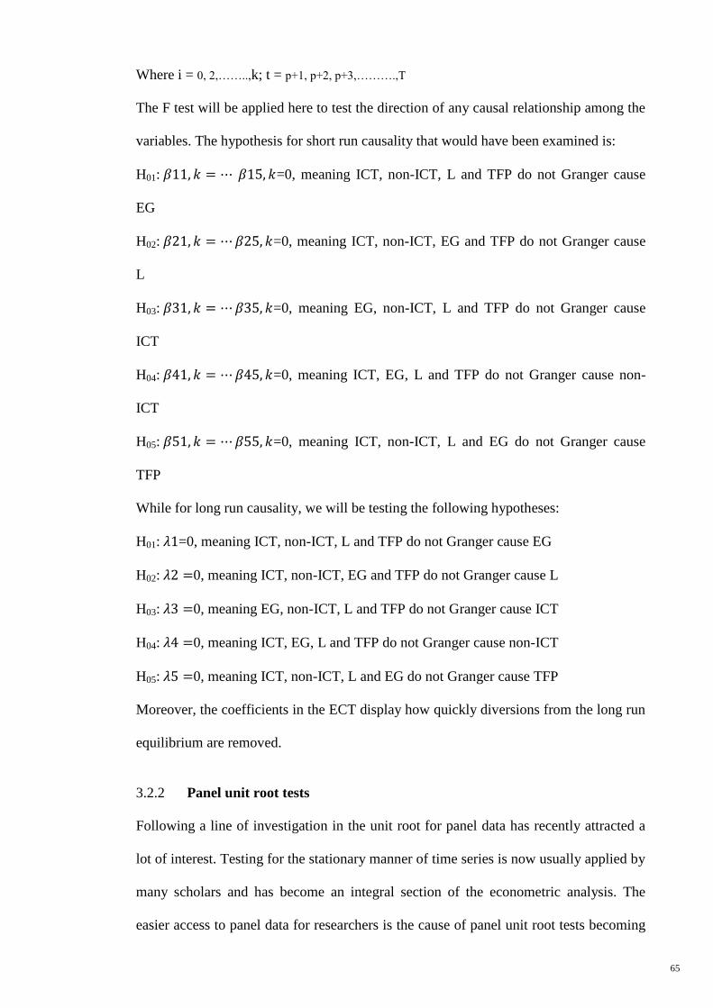
65

Where i = 0, 2,……..,k; t = p+1, p+2, p+3,……….,T

The F test will be applied here to test the direction of any causal relationship among the

variables. The hypothesis for short run causality that would have been examined is:

H01: =0, meaning ICT, non-ICT, L and TFP do not Granger cause

EG

H02: =0, meaning ICT, non-ICT, EG and TFP do not Granger cause

L

H03: =0, meaning EG, non-ICT, L and TFP do not Granger cause

ICT

H04: =0, meaning ICT, EG, L and TFP do not Granger cause non-

ICT

H05: =0, meaning ICT, non-ICT, L and EG do not Granger cause

TFP

While for long run causality, we will be testing the following hypotheses:

H01: =0, meaning ICT, non-ICT, L and TFP do not Granger cause EG

H02: 0, meaning ICT, non-ICT, EG and TFP do not Granger cause L

H03: 0, meaning EG, non-ICT, L and TFP do not Granger cause ICT

H04: 0, meaning ICT, EG, L and TFP do not Granger cause non-ICT

H05: 0, meaning ICT, non-ICT, L and EG do not Granger cause TFP

Moreover, the coefficients in the ECT display how quickly diversions from the long run

equilibrium are removed.

3.2.2 Panel unit root tests

Following a line of investigation in the unit root for panel data has recently attracted a

lot of interest. Testing for the stationary manner of time series is now usually applied by

many scholars and has become an integral section of the econometric analysis. The

easier access to panel data for researchers is the cause of panel unit root tests becoming

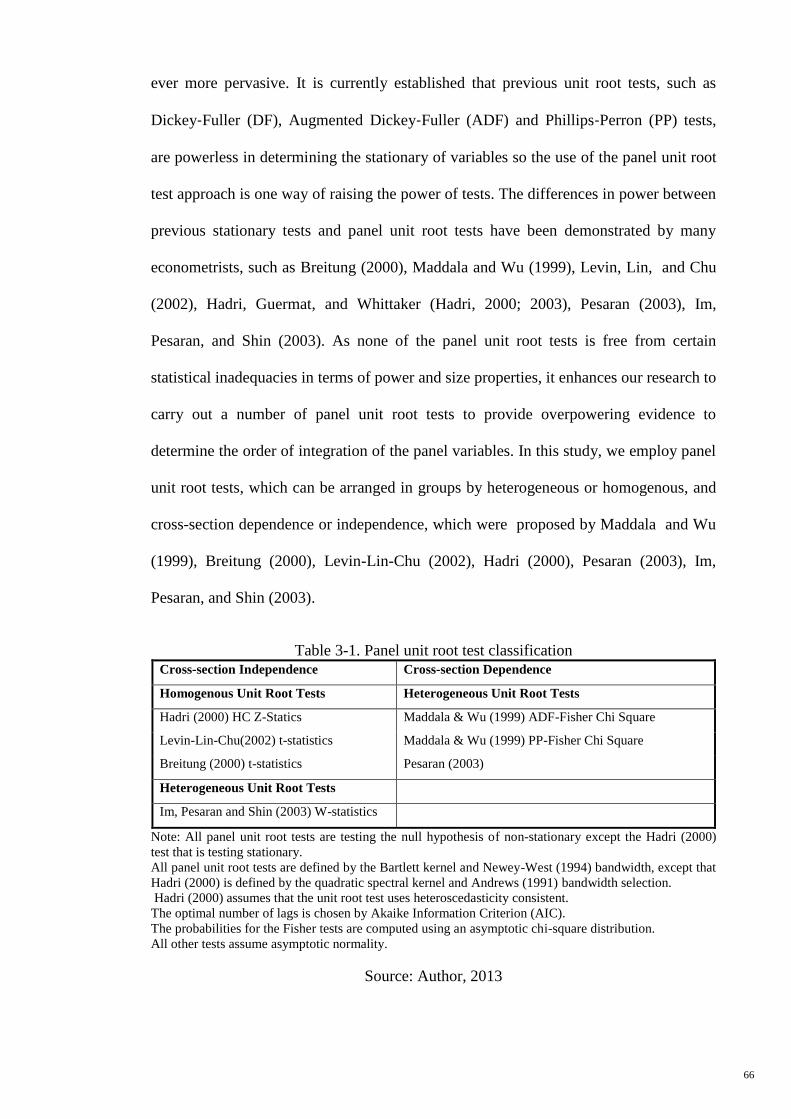
66

ever more pervasive. It is currently established that previous unit root tests, such as

Dickey‐Fuller (DF), Augmented Dickey‐Fuller (ADF) and Phillips‐Perron (PP) tests,

are powerless in determining the stationary of variables so the use of the panel unit root

test approach is one way of raising the power of tests. The differences in power between

previous stationary tests and panel unit root tests have been demonstrated by many

econometrists, such as Breitung (2000), Maddala and Wu (1999), Levin, Lin, and Chu

(2002), Hadri, Guermat, and Whittaker (Hadri, 2000; 2003), Pesaran (2003), Im,

Pesaran, and Shin (2003). As none of the panel unit root tests is free from certain

statistical inadequacies in terms of power and size properties, it enhances our research to

carry out a number of panel unit root tests to provide overpowering evidence to

determine the order of integration of the panel variables. In this study, we employ panel

unit root tests, which can be arranged in groups by heterogeneous or homogenous, and

cross-section dependence or independence, which were proposed by Maddala and Wu

(1999), Breitung (2000), Levin-Lin-Chu (2002), Hadri (2000), Pesaran (2003), Im,

Pesaran, and Shin (2003).

Table 3-1. Panel unit root test classification

Cross-section Independence Cross-section Dependence

Homogenous Unit Root Tests Heterogeneous Unit Root Tests

Hadri (2000) HC Z-Statics Maddala & Wu (1999) ADF-Fisher Chi Square

Levin-Lin-Chu(2002) t-statistics Maddala & Wu (1999) PP-Fisher Chi Square

Breitung (2000) t-statistics Pesaran (2003)

Heterogeneous Unit Root Tests

Im, Pesaran and Shin (2003) W-statistics

Note: All panel unit root tests are testing the null hypothesis of non-stationary except the Hadri (2000)

test that is testing stationary.

All panel unit root tests are defined by the Bartlett kernel and Newey-West (1994) bandwidth, except that

Hadri (2000) is defined by the quadratic spectral kernel and Andrews (1991) bandwidth selection.

Hadri (2000) assumes that the unit root test uses heteroscedasticity consistent.

The optimal number of lags is chosen by Akaike Information Criterion (AIC).

The probabilities for the Fisher tests are computed using an asymptotic chi-square distribution.

All other tests assume asymptotic normality.


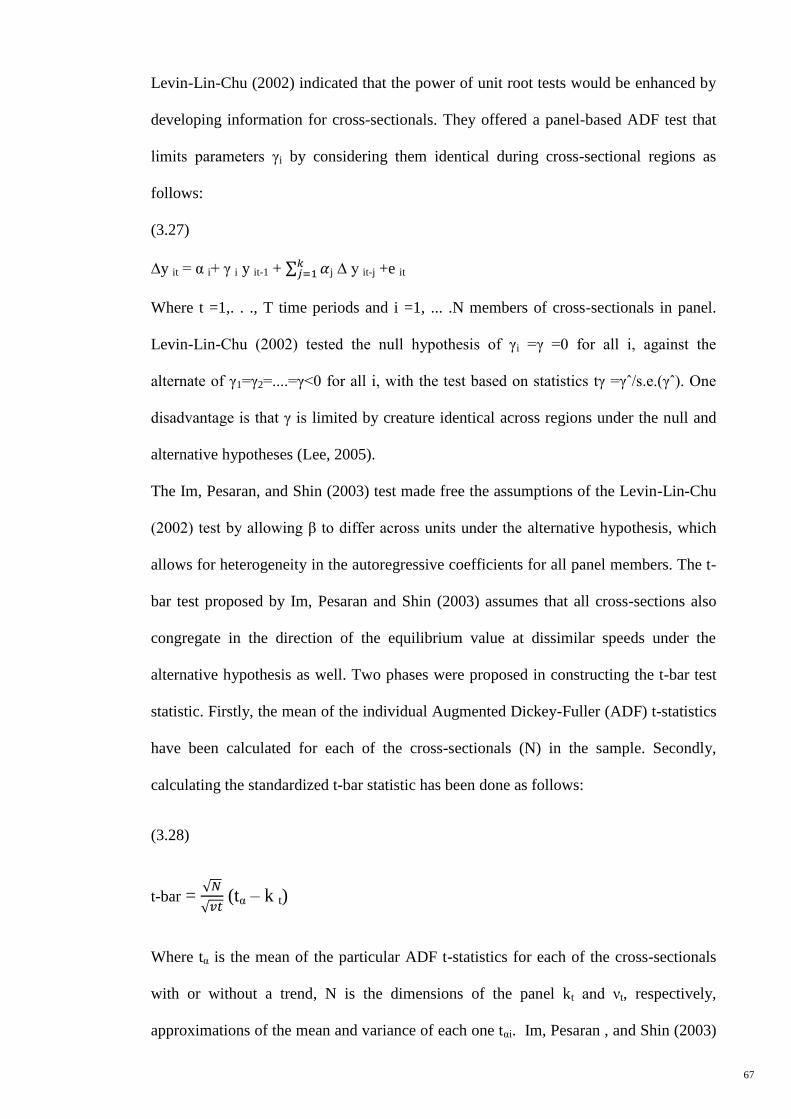
67

Levin-Lin-Chu (2002) indicated that the power of unit root tests would be enhanced by

developing information for cross-sectionals. They offered a panel-based ADF test that

limits parameters γi by considering them identical during cross-sectional regions as

follows:

(3.27)

∆y it = α i+ γ i y it-1 + j ∆ y it-j +e it

Where t =1,. . ., T time periods and i =1, ... .N members of cross-sectionals in panel.

Levin-Lin-Chu (2002) tested the null hypothesis of γi =γ =0 for all i, against the

alternate of γ1=γ2=....=γ<0 for all i, with the test based on statistics tγ =γˆ/s.e.(γˆ). One

disadvantage is that γ is limited by creature identical across regions under the null and

alternative hypotheses (Lee, 2005).

The Im, Pesaran, and Shin (2003) test made free the assumptions of the Levin-Lin-Chu

(2002) test by allowing β to differ across units under the alternative hypothesis, which

allows for heterogeneity in the autoregressive coefficients for all panel members. The t-

bar test proposed by Im, Pesaran and Shin (2003) assumes that all cross-sections also

congregate in the direction of the equilibrium value at dissimilar speeds under the

alternative hypothesis as well. Two phases were proposed in constructing the t-bar test

statistic. Firstly, the mean of the individual Augmented Dickey-Fuller (ADF) t-statistics

have been calculated for each of the cross-sectionals (N) in the sample. Secondly,

calculating the standardized t-bar statistic has been done as follows:

(3.28)

t-bar =

(tα – k t)

Where tα is the mean of the particular ADF t-statistics for each of the cross-sectionals

with or without a trend, N is the dimensions of the panel kt and νt, respectively,

approximations of the mean and variance of each one tαi. Im, Pesaran , and Shin (2003)

68

presented Monte Carlo simulations of kt and νt and accurately tabulated critical values

for a range of combinations of N and T. A challenge with the t-bar test is the fact that

the test is simply not applicable if there is cross-sectional dependency in the

disturbances. Nevertheless, Im, Pesaran, and Shin (2003) advised that in the presence of

cross-sectional dependency, the data might be modified by demeaning that the

standardized demeaned t-bar statistic congregates to the standard normal in the control.

An optional technique to the panel unit root tests is to apply Fisher’s (1925) method to

obtain results that merge the p-values of individual unit root tests. Subsequent to the

Fisher (1925) test, Maddala and Wu (1999), based on the Fisher (1925) test, provided a

non-parametric test statistic. This test primarily synthesizes the p-values of a particular

unit root test in any residual cross-sectional unit. The test is a sort of non-parametric test

and includes a chi-square distribution with 2N levels of freedom, whereas N is the

number of countries or cross-sectional units. The following test statistic tends to be

obtained by applying the additive property of the chi-squared variable:

(3.29)

λ = -2 e πi

Where, πi is the p-value of the test statistic for unit i. One of the advantages of the

Maddala and Wu (1999) test on the Im, Pesaran and Shin (2003) test is that it is

independent on different lag lengths in the individual ADF regressions. Maddala and

Wu (1999) carried out Monte Carlo simulations presenting which is better to that

proposed by Im, Pesaran and Shin (2003).

Another panel unit root test proposed by Breitung (2000) is a recent large-scale Monte

Carlo simulation presented by Narayan and Smyth (2009). They found that the Breitung

(2000) panel unit root test commonly had the maximum power and least size bend of

every test that are called first generation panel unit root tests. The following equation is

the Breitung (2000) panel unit root test:

69

(3.30)

Yit = α it+ ik Xi,t-k + εt

The Breitung (2000) test employs equation (30) to test statistics under the following null

hypothesis that the process has a unit root: H0: ik -1 = 0. The alternative

hypothesis assumes that the panel series does not have a unit root; that is, ik -1 < 0

for all i. The following transformed vectors to extract the test statistic are used by

Breitung (2000):

(3.31)

Y*i= A Y i =[y*i1, y*i2,… ,y*iT]'

(3.32)

X*i = A Xi = [x*i1,x*i2,…,x*iT]'

These lead to the following test statistic:

(3.33)

λβ =

This is expected to have a normal standard distribution (Mishra, Smyth, & Sharma,

2009). The results of the panel unit root tests are reported in chapter 4. The test statistics

for the majority of level variables are statistically insignificant with some exceptions

that we will deal with in detail in chapter 4. Considered an entity, the level outcomes

endorse that all the variables are panel non-stationary; consequently, we employ the

panel unit root tests to the first difference of variables.

However, Hadri (2000) proposed that the null hypothesis has to be reversed to be the

stationary hypothesis to establish a more robust test. The Lagrange Multiplier (LM)

statistic for Hadri’s (2000) test could be written as:

(3.34)

LˆM =

ε

70

where σˆ2 is in line with Newey and West’s (1987) estimation of the long run variance

of disturbance terms (Lee, 2005).

Several panel unit root tests are offered. In our empirical analysis, we will use a recent

panel unit root test improved by Pesaran (2003), which has accounted for cross-

sectional dependence. Based on the applied economics literature, given that this test is

comparatively new and less used it has provided some additional information

concerning this test. Pesaran (2003) built a panel unit root test by improving the

augmented Dickey-Fuller (ADF) regression with cross-sectional means of first

differences and lagged levels of the individual series. This test is named as the cross-

sectional augmented ADF (CADF) test, which assumes that all series are non-stationary

under the null hypothesis. The following regression represents the CADF test here.

(3.35)

∆ yit = α i +βi y it-1 +ηi y¯t +ki∆ y¯t+εit

Where, y¯

t is the average of the variable yt. Amount of null hypothesis to test the unit

root is H0: βi = 0 for all i. Against the probable alternative hypothesis H1: βi< 0, i=

1,2,…,N1, βi =0, i=N1+1, N1+2,…,N

To examine the null hypothesis, the t-test has been employed. The distribution is not

normal/abnormal, whereas critical values are produced by Pesaran8 (2003) as well as

Narayan, Narayan, and Popp (2010).

3.2.3 Panel cointegration tests

Since we extracted Solow’s Residual as a measure of productivity, we need to examine

the causal relationship between the value added growth (Y in the equations) and ICT,

Solow’s Residual (A in the equations), labour and non-ICT. To analyse the long run

relationship between variables, we employed the vector error correction model (VECM)

and system generalized moment of method (GMM) in panel data analysis. Over time

8More technical details can be found in Pesaran M.H. "A simple panel unit root test in the presence of cross-section dependence”. J

Appl Econom 2007; 22:265–312.

71

series studies, two variables are supposed to have a long run relationship whether they

are cointegrated. We are able to estimate the variables in equation (2) to be

cointegrated, if the order of integration of the left hand side variable (economic growth)

would be equal to or larger than the highest order of integration of the right hand side

variables (K, L, ICT, non-ICT and TFP). Otherwise, even without cointegration tests,

they are clearly not cointegrated.

Before the cointegration test, we carried out the panel unit root tests to determine the

order of integration of the variables. This test was helpful to identify stationary

variables for the Granger causality test. According to the results of the Hausman and F-

tests, we developed the vector error correction model (VECM) by employing the pooled

mean group (PMG), mean group (MG), and dynamic fixed effect (DFE) estimators to

identify the causal relationship among variables. The concept of cointegration was first

made popular by Granger (1981) and improved further by Engle and Granger (1987);

Johansen (1988, 1991) and Phillips and Ouliaris (1990), among others. The fundamental

concept is that if two or more time series variables are individually integrated of order n,

then there is a possibility of at least one linear combination to be integrated of a lower

order than n.

Therefore, such a relationship between these variables concludes cointegration.

Cointegrated variables display a strong stable‐state relationship in the long run, having

general trends and co‐movements similar to panel unit root tests. By extension of the

time series cointegration tests to panel cointegration, two groups of tests have been

proposed: the first group of tests considers cointegration as the null hypothesis

(McCoskey & Kao, 1998; Westerlund & Edgerton, 2007) whereas the other group of

tests considers no cointegration as the null hypothesis (Pedroni, 1999; Kao, Chiang &

Chen, 1999; Groen & Kleibergen, 2003; Larsson, Lyhagen & Löthgren, 2008).

72

Once the presence of a panel unit root has been recognized, the concern arises as to

whether there is a long run equilibrium relationship among the regressors. In the current

research, we have used two methods of panel cointegration test. The first set of tests is

proposed by Pedroni (2004). The second set is from Kao (1999), which is the

generalized Augmented Dickey-Fuller (ADF) tests in the panel data framework. These

two tests have shown no cointegration possibility under the null hypothesis while

employing the residuals comprising of a panel regression to make the test statistics and

establish the distributions.

Pedroni’s cointegration test methodology like the Im, Pesaran and Shin (2003) test, is a

heterogeneous panel cointegration test that was improved by Pedroni (1999, 2004)

allowing cross-sectional interdependence with different individual effects. The

following equation presents the empirical model of Pedroni’s cointegration test.

(3.35)

Yit = η i + δit+ i Xit + εit

Where i=0,1,2,…,N for each country or industry in the panel and t=0,1,2,…..,T denotes

the time period; Y, and X are dependent and independent variables. ηi and δi are country

or industry and time fixed effects, respectively (Uysal, 2010). A deviation from the long

run relationship is accounted for by εit, which is estimated by residuals. The estimated

residuals are structured as follows:

(3.36)

εît=ρî εît-1+uît

Seven different statistics to test the panel data long run relationship were proposed by

Pedroni (1999, 2004). Of these seven statistics, three of them are known as the

73

‘‘between’’ dimension and the other four depend on pooling what is represented as the

‘‘within’’ dimension. Both types test the null hypothesis of no cointegration. However,

the differences come from the design of the alternative hypothesis, which is testing the

alternative hypothesis ρi = ρ <1 on ‘‘within’’, for all i, while concerns based on the

‘‘between’’ dimension, the alternative hypothesis is ρi <1 for all i. Pedroni (1999) used

Monte Carlo simulations in tabulating the finite sample distribution of seven test

statistics. The established statistic tests have to be larger than the tabulated critical value

not to reject the null hypothesis of absence of cointegration.

A drawback of the tests offered by Pedroni (1999) is that it is established on the

hypothesis of overall factor limitation and that it cannot take feasible cross-country

dependency into account. This hypothesis proposes that the short run parameters of the

factors in their first differences are equivalent to the long run parameters for the

variables in their levels. A failure to suit the limitation leads to a significant decrease of

power for the residual based panel cointegration tests (Eggoh, Bangake, & Rault, 2011).

In this research, in addition to applying the Pedroni (2004, 1999) tests, we also use the

panel cointegration tests proposed by Kao (1999) to examine the relationship between

the variables. The following regression equation presents the measurement of the Kao

(1999) ADF type test.

(3.37)

eit = ρ eit-1 +

Where eit’s are the estimated residuals from the panel static regression equation;

(3.38)

Yit=µi+ Xit´ β+ uit; i=1,2,…..,N: t=1,2,…..T

The alternative hypothesis is H1: ρ< 1, against the null hypothesis of no cointegration is

H0: ρ = 1.

74

3.2.4 Panel Error Correction Model (ECM)

The idea of cointegration can be clear as an efficient co-movement among two or more

economic variables in the long run. Due to the Engle and Granger (1987) procedure, if

the X and Y as variables are both non-stationary, one possibility could expect that a

linear approximation of X and Y would be a random walk. However, the two variables

may have the characteristic that a particular combination of them Z=X-bY is stationary.

Consequently, if such a property holds true, then we profess that X and Y are

cointegrated. If X and Y are both non-stationary and the linear combination of two

variables is also non-stationary, then the standard Granger causality test should be

applicable. Whereas, if X and Y are both non-stationary and cointegrated, then any

standard Granger causal inferences will give misleading results, and, thus, a more

comprehensive causality test based on an error correction model (ECM) must be applied

(Toda & Phillips, 1993).

Our panel data has been set at the industrial level consisting of 21 industries for the

period 1990-2007 and at the national level consisting of six countries for the period

1990-2011. The use of an ECM model is mostly suggested in cases in which the time

observation (T) is large or both time observations (T) and cross-sectional observations

(N) are approximately a similar order of size. This estimator can be practical for

separating the short run from the long run effects, which would allow us to estimate the

long run impact of ICT on output growth. Our empirical process is composed of (i)

evaluating the stationary of the panel variables, (ii) in case the variables are not

stationary, we tested for the existence of a cointegrating relationship and (iii) in case

cointegration is acknowledged, we are able to carry on by estimating an ECM model.

The assessments employed to check for stationary and cointegration are discussed in the

results and discussion sections. In this section, we employ the panel ECM using the

75

econometric approach. Firstly, the following Autoregressive Distributed Lag Model

ARDL (p, q) model is considered for T periods and N industries or countries:

(3.39):

Yit= +

Where Y is output, X is the vector of the independent variables, are fixed effects for

each industry or country, are the coefficients of the lagged dependent variables

and are coefficients of current and lagged independent variables. This model yields

the following ECM form:

(3.40)

∆Yit= +

Where βi is the long run parameter for each N, γij are the short run coefficients and i

are the ECT parameters. Imposing common β coefficients across industries or countries:

(3.41)

∆Yit= +

Three currently developed techniques for estimating this sort of model, as suggested by

Pesaran et al. (1999), are the mean group (MG), the pooled mean group (PMG), and

dynamic fixed effect (DFE) estimators. Such panel data estimators are extremely highly

recommended in cases that the time point of view (T) is massive or both time

observations (T) and cross-sectional observations (N) are approximately a similar order

of size. In the long run, with conventional fixed effect estimators, homogeneity of slope

coefficients is assumed, while the Mean Group (MG) estimators enable the slopes and

intercepts to differ over the cross-sectionals. The Mean Group (MG) estimates the

coefficients across each one cross-section and then needs the mean thereof.

The Pooled Mean Group (PMG) estimators combine the fixed effects and Mean Group

(MG) that permit the short run coefficients to change; however, enforce long run

76

coefficients are equal across sections (N). Hence, the PMG estimator makes it possible

for us to estimate a usual long run relationship across sections without notable restricted

assumptions of same short run dynamics across sections. Dynamic Fixed Effect (DFE)

estimators, like the Pooled Mean Group (PMG) estimators, restrict the coefficients of

the long run vector to be equal across all panels (Blackburne & Frank, 2009).

There is a consistency-efficiency trade-off in choosing among MG, PMG, and DFE.

While the MG estimators provide consistent estimates of the PMG estimators, they are

significantly less efficient in comparison to the mean of the long run coefficients. The

PMG estimators are consistent and efficient, when the homogeneity of the long run

coefficients is retained. Additionally, the DFE model limits the speed of the adjusted

coefficient (ECT) and the short run coefficients to be equivalent, whereas the PMG

estimator depends on a combination of pooling and averaging of coefficients. To

identify which estimator may be more suitable, we generally rely on the Hausman

(1981) specification test and F-test. While we will explain the findings in Chapter 4,

various methods are selected among countries and industries.

3.2.5 System GMM and first-difference GMM

The main panel data estimation methods are centred on both random and fixed effect

models. It is usually applied to simultaneous accounts that have the presence of time-to-

time fluctuations and heterogeneity in the economic performance of cross-sections. In

this mean, we discovered that several of the explanatory variables included in the

industrial and aggregate level regressions are either endogenous or pre-determined, thus

confounding the results.

For instance, as mentioned in section 1.2.5, considering that ICT capital is of an

endogenous nature as a General Purpose Technology (GPT), it means that it is very

likely that it will have external growth impacts, particularly with lags. This has two

meanings: (1) that there might be a dynamic route to ICT’s growth impact, so it will

77

only be in the long run that their effects will arise and (2) that there would be a

correlation of ICT capital with the error term. Therefore, ICT capital is expected to be

an endogenous covariate. Other explanatory variables, like Labour, TFP and Non-ICT,

future understanding may be affected due to output growth historical data so that a

partial influence might not be orthogonal to the error term of the regression of these

variables.

In this situation, biased and inconsistent results are expected to be produced due to the

traditional panel data estimation methods (either the random or the fixed effect

estimators). New estimation techniques, such as first-difference and System GMM

panel data estimators (Arellano & Bover, 1995; Blundell & Bond, 1998) are appropriate

due to the correlation between the explanatory variables and historical or even current

realizations of the error term (Roodman, 2008).

An unobservable country specific effect is another estimation difficulty in growth

equilibriums whose presence has been established in our study. The GMM estimator is

also used in an attempt to overcome this problem. Accordingly, a decision is needed as

to which variable should be employed as an instrumental variable.

GMM estimators are quite useful in the estimation of panel data with a relatively small

time dimension (T) comparative to the number (N) of cross-sections (Roodman, 2008).

In contrast, as time observations become greater, misleading and inconsistent coefficient

estimates would be provided by the GMM estimator, unless the slope coefficients are

equal across cross-sections (Pesaran & Smith, 1995). Through the estimation of separate

regression, the problem has been addressed in this study in aggregate level through the

use of a comparatively large time dimension (N = 6, T = 22) for the sub-periods of

1990-2000 and 2001-2011. However, for the industrial level study the time observation

is relatively smaller, therefore the whole period of panel has been run in this study. This

78

has enabled us to examine the varying effects of ICT across time, and its spillover

effects.

It is clear that the augmented extension of the Arellano and Bond (1991) first-difference

GMM estimator is the System GMM estimator, which uses endogenous variables

lagged levels as instruments. Sometimes the regressor lagged levels are not powerful

instruments for the first-differenced GMM regressor. In this case, one should employ

the augmented version “System GMM”. Generally, the level equation is used to achieve

a system of two equations by the System GMM: one in levels and one in differenced.

By adding the second equation, supplementary instruments can be gained. Therefore,

the variables in levels in the second equation are instrumented with their own first

differences, which are usually increasing efficiency.

In conclusion, the System GMM estimators employ the first differences of the

instrumented variables as additional instruments. As argued by Arellano and Bover

(1995), and Blundell and Bond (1998), the allowance of more instruments in this

System GMM estimator can dramatically improve the efficiency of the obtained

estimates.

Accordingly, we choose the System GMM in the industrial level data in this research,

while we use the first-difference GMM for the aggregate level in this study for two

important reasons to be made about using first-difference GMM. First, because System

GMM uses more instruments than the difference GMM, it may not be appropriate to

employ System GMM with a dataset comprising a small number of countries (aggregate

level data with N=6, T=11) (Mileva, 2007). Therefore, we intend to use first-difference

GMM for the aggregate level part of the study and System GMM for the industrial level

part with large cross-sectional data (N=21, T=17).

In this regard, we employ the System GMM panel data estimator in order to tackle the

issue of the endogeneity of repressors in the industrial level panel data with large N

79

(number of industries =21). Next, we quantify the growth effects of ICT by employing

the first-difference GMM developed by Arellano and Bond (1991) at the aggregate level

that addresses the above-mentioned problems more effectively and obtain robust

estimates in the first and two steps for six countries in each group. In this method,

lagged values of the dependent and explanatory variables are used as instruments.

The GMM estimator, either the first difference or the system version, has one and two-

step variants. The two-step estimator is considered as more efficient; however, the

standard errors are downward biased and render GMM estimates useless for inference

(Arellano & Bond, 1991). This problem is mitigated in the System GMM version

because it incorporates the finite sample correction to the two-step covariance matrix.

For this reason, our basic analysis is based on regression, which uses two-step GMM

estimators.

The GMM estimators report two diagnostic tests. The first one is the Sargan and Hansen

test, which checks for the validity of normal-type instruments and GMM-type

instruments. The hypothesis being tested with the Hansen and Sargan tests is that the

two types of instruments are uncorrelated with the residuals, and, therefore, are

acceptable instruments. If the null hypothesis is confirmed statistically (not rejected),

the instruments leave behind the test and are considered valid by this criterion. These

estimators also represent a test for serial correlation, which is applied to the first

differenced residuals and upper differences. If the null of no autocorrelation is rejected

then the test points out that lags of the used instruments are in fact endogenous and are

consequently considered ‘bad’ instruments.

With respect to the number of lags used in the GMM regressions, it is generally

adequate that as the number of lags grows, the likelihood of finding proper instruments

increases. On the other hand, when the number of moment conditions expands, this

80

leads to a decrease in the size of the sample, bias in the estimates and less power of the

diagnostic tests (Roodman, 2008).

To sum up, as pointed out by Roodman (2008), the Arellano and Bond (1991), Arellano

and Bover (1995), Blundell and Bond (1998) dynamic panel estimators are

progressively more popular. All are common estimators designed for situations with 1)

“small T, large N" panels, means few time observations and lots of individuals; 2) a

linear functional model; 3) a single left-hand-side variable that is dynamic, depending

on its own past observations; 4) explanatory variables that are not strictly exogenous,

means correlated with past and possibly current observations of the error term; 5)

heteroscedasticity and autocorrelation within individuals but not between them; and 6)

fixed individual effects.

The Arellano and Bond (1991) estimation starts by transforming all regressors, usually

by differencing and using the Generalized Method of Moments condition, that is called

the first-difference GMM. The Arellano and Bover (1995) and Blundell and Bond

(1998) estimator augments Arellano and Bond (1991) by creating a supplementary

assumption, that the first differences of the instrument variables are uncorrelated with

the fixed effects. As a result, allowing introducing more instruments can considerably

improve efficiency. It constructs a system of two equations, the original equation as

well as the transformed one and is well known as System GMM (Roodman, 2008). In

addition, diagnostic tests like over-identification tests and serial correlation tests are

applied to ensure there is no bias due to correlation with the error term.

81

4 CHAPTER 4: RESULTS AND DISCUSSION

4.1 Introduction

The discussion in the econometric methodology section demonstrated that ICT capital is

considered as General Purpose Technology (GPT) of an endogenous nature, meaning it

will most likely have external growth effects, particularly with lags. This means that the

process of growth due to the impact of ICT might be dynamic, thus it will only be in the

long run that its impact will surface. In addition, there might be a correlation between

ICT capital and error-term.

It appears that because of the endogeneity problem, it is most likely that inconsistent

and biased results would be produced via using traditional panel data estimation

methods (either the random effect or fixed estimator). In this study, we apply newly

developed panel data techniques to quantify the impact on growth of ICT. Firstly, the

panel error correction model is estimated to assess the short run and long run effects on

output growth by ICT. This approach is commonly used for the detection of causal

relationships between variables by applying the Engle-Granger test procedure. To

estimate non-stationary dynamic panels, we have used three new techniques – Pooled

Mean Group (PMG) estimators, the Dynamic Fixed Effect (DFE) estimators and Mean

Group (MG) (M.H. Pesaran, Shin, & Smith, 1999). For the analysis of panel data with

time series (T) and cross-section (N), which are of the same order of magnitude and are

relatively large, panel data estimators are particularly useful (Blackburne & Frank,

2009).

Before implementation of ECM, we have tested for the presence of unit root in panels,

and the issue arises as to whether there is an existence of a long run equilibrium

relationship between the variables. Two sets of panel cointegration test methods are

used in our empirical analysis. Pedroni (2004) proposed the first set of tests. A

generalised Augmented Dickey-Fuller (ADF) test is the second set of tests proposed by

82

Kao (1999) in the panel data framework. The results of these two tests have suggested

no possibility of cointegration under the null hypothesis while employing the residuals

derived from a panel regression so as to establish the distributions and make the test

statistics.

Next, in order to overcome the issue of endogeneity in the long run causal relationship

between ICT and economic growth, system GMM and first-difference GMM panel data

estimator will be used. We will assess the value added growth at the aggregate level,

through TFP and some controlling variables in order to cover the spillover effects of

ICT by using System GMM as well.

4.2 Reasons for Choice of Countries

The main purpose of this research is to assess the comprehensive ICT effects on

economic growth with regards to the top ICT developed countries in Asia-Pacific and

Europe. According to the literature, there are many works on comparative studies on the

EU and US. In these studies, the ICT development index has been disregarded,

especially in Asia-Pacific countries at the industrial level panels. To fill this gap, we

collect aggregate level data for 12 top ranked ICT developed countries in EU and Asia-

Pacific countries from the World Bank Indicator (WDI) database. To execute the same

analysis at the industrial level we have some limitations in the data collection process.

In Asia-Pacific countries, from the six top ranked ICT developed countries, as

illustrated in Table 4-1, we only succeeded in collecting data for Japan and Australia. In

the EU zone countries, from the six top ranked ICT developed countries, as illustrated

in Table 4-1, we only succeeded in collecting data for Sweden, Denmark, and Finland.

This study relies on the International Telecommunication Union (ITU) in the 2010

ranking of ICT developed countries. To be more precise, we have used the EU KLEMS

database as the unique database in order to capture high reliability for our datasets.

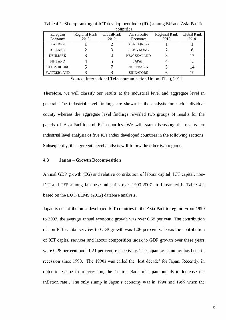
83

Table 4-1. Six top ranking of ICT development index(IDI) among EU and Asia-Pacific

countries

European

Economy

Regional Rank

2010

GlobalRank

2010

Asia-Pacific

Economy

Regional Rank

2010

Global Rank

2010



DENMARK 3 4 NEW ZEALAND 3 12





Therefore, we will classify our results at the industrial level and aggregate level in

general. The industrial level findings are shown in the analysis for each individual

county whereas the aggregate level findings revealed two groups of results for the

panels of Asia-Pacific and EU countries. We will start discussing the results for

industrial level analysis of five ICT index developed countries in the following sections.

Subsequently, the aggregate level analysis will follow the other two regions.

4.3 Japan – Growth Decomposition

Annual GDP growth (EG) and relative contribution of labour capital, ICT capital, non-

ICT and TFP among Japanese industries over 1990-2007 are illustrated in Table 4-2

based on the EU KLEMS (2012) database analysis.

Japan is one of the most developed ICT countries in the Asia-Pacific region. From 1990

to 2007, the average annual economic growth was over 0.68 per cent. The contribution

of non-ICT capital services to GDP growth was 1.06 per cent whereas the contribution

of ICT capital services and labour composition index to GDP growth over these years

were 0.28 per cent and -1.24 per cent, respectively. The Japanese economy has been in

recession since 1990. The 1990s was called the ‘lost decade’ for Japan. Recently, in

order to escape from recession, the Central Bank of Japan intends to increase the

inflation rate . The only slump in Japan’s economy was in 1998 and 1999 when the

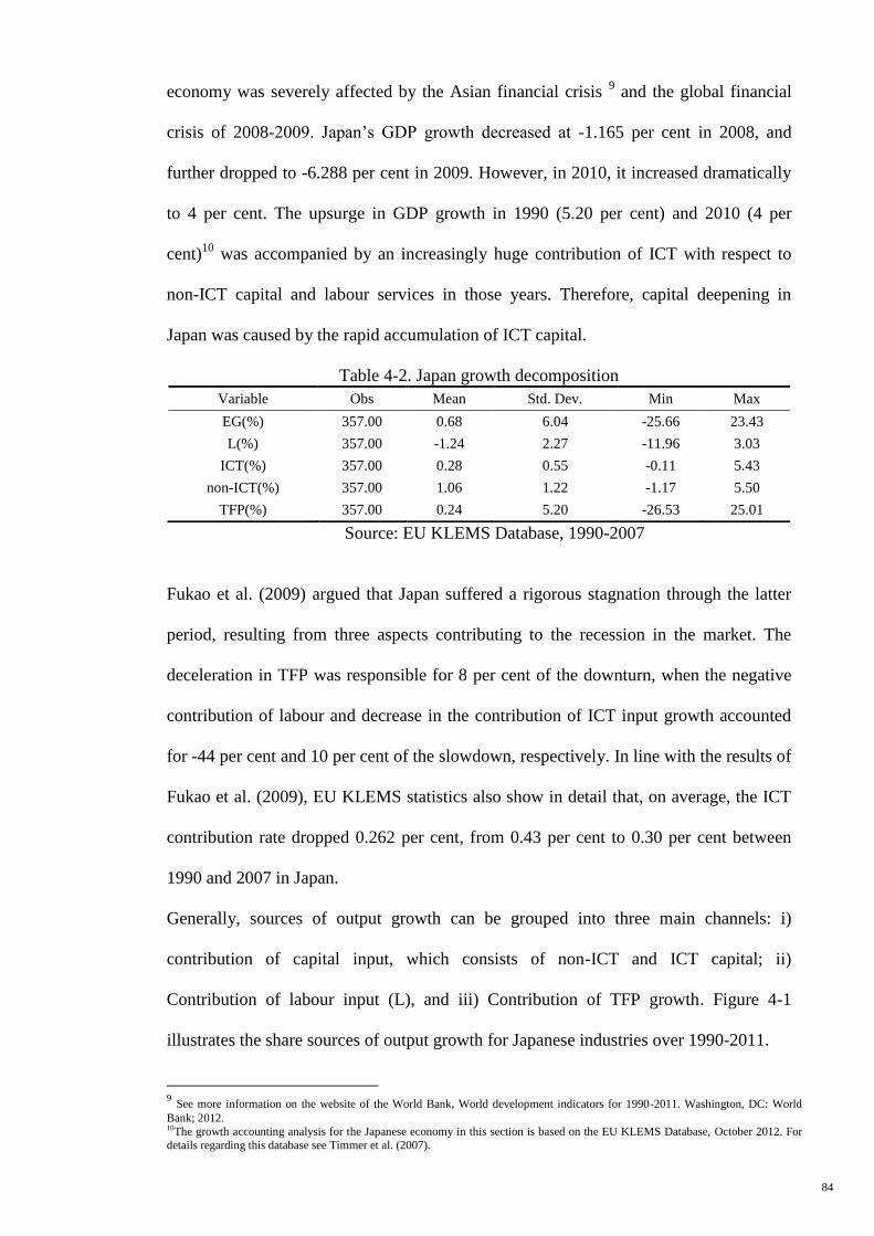
84

economy was severely affected by the Asian financial crisis 9 and the global financial

crisis of 2008-2009. Japan’s GDP growth decreased at -1.165 per cent in 2008, and

further dropped to -6.288 per cent in 2009. However, in 2010, it increased dramatically

to 4 per cent. The upsurge in GDP growth in 1990 (5.20 per cent) and 2010 (4 per

cent)10

was accompanied by an increasingly huge contribution of ICT with respect to

non-ICT capital and labour services in those years. Therefore, capital deepening in

Japan was caused by the rapid accumulation of ICT capital.

Table 4-2. Japan growth decomposition

Variable Obs Mean Std. Dev. Min Max

EG(%) 357.00 0.68 6.04 -25.66 23.43

L(%) 357.00 -1.24 2.27 -11.96 3.03

ICT(%) 357.00 0.28 0.55 -0.11 5.43

non-ICT(%) 357.00 1.06 1.22 -1.17 5.50

TFP(%) 357.00 0.24 5.20 -26.53 25.01

Source: EU KLEMS Database, 1990-2007

Fukao et al. (2009) argued that Japan suffered a rigorous stagnation through the latter

period, resulting from three aspects contributing to the recession in the market. The

deceleration in TFP was responsible for 8 per cent of the downturn, when the negative

contribution of labour and decrease in the contribution of ICT input growth accounted

for -44 per cent and 10 per cent of the slowdown, respectively. In line with the results of

Fukao et al. (2009), EU KLEMS statistics also show in detail that, on average, the ICT

contribution rate dropped 0.262 per cent, from 0.43 per cent to 0.30 per cent between

1990 and 2007 in Japan.

Generally, sources of output growth can be grouped into three main channels: i)

contribution of capital input, which consists of non-ICT and ICT capital; ii)

Contribution of labour input (L), and iii) Contribution of TFP growth. Figure 4-1

illustrates the share sources of output growth for Japanese industries over 1990-2011.

9 See more information on the website of the World Bank, World development indicators for 1990-2011. Washington, DC: World

Bank; 2012. 10The growth accounting analysis for the Japanese economy in this section is based on the EU KLEMS Database, October 2012. For

details regarding this database see Timmer et al. (2007).

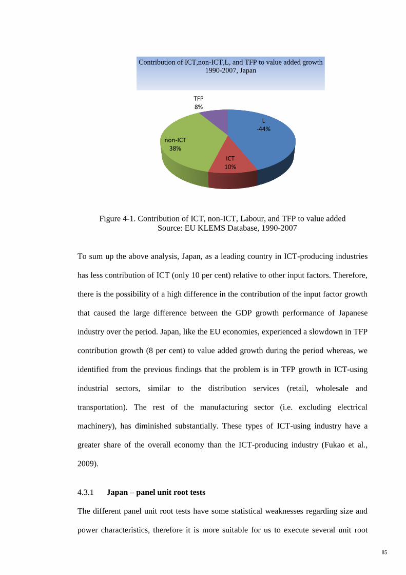
85

Figure 4-1. Contribution of ICT, non-ICT, Labour, and TFP to value added


To sum up the above analysis, Japan, as a leading country in ICT-producing industries

has less contribution of ICT (only 10 per cent) relative to other input factors. Therefore,

there is the possibility of a high difference in the contribution of the input factor growth

that caused the large difference between the GDP growth performance of Japanese

industry over the period. Japan, like the EU economies, experienced a slowdown in TFP

contribution growth (8 per cent) to value added growth during the period whereas, we

identified from the previous findings that the problem is in TFP growth in ICT-using

industrial sectors, similar to the distribution services (retail, wholesale and

transportation). The rest of the manufacturing sector (i.e. excluding electrical

machinery), has diminished substantially. These types of ICT-using industry have a

greater share of the overall economy than the ICT-producing industry (Fukao et al.,

2009).

4.3.1 Japan – panel unit root tests

The different panel unit root tests have some statistical weaknesses regarding size and

power characteristics, therefore it is more suitable for us to execute several unit root

L -44%

ICT 10%

non-ICT 38%

TFP 8%

Contribution of ICT,non-ICT,L, and TFP to value added growth

1990-2007, Japan

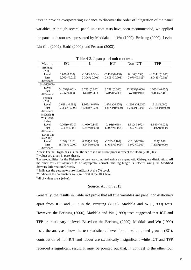
86

tests to provide overpowering evidence to discover the order of integration of the panel

variables. Although several panel unit root tests have been recommended, we applied

the panel unit root tests presented by Maddala and Wu (1999), Breitung (2000), Levin-

Lin-Chu (2002), Hadri (2000), and Pesaran (2003).

Table 4-3. Japan panel unit root tests

Method EG L ICT Non-ICT TFP Breitung

(2000)

Level

First

difference

0.076(0.530)

-2.262*(0.012)

-0.348( 0.364)

-3.306*( 0.001)

-2.406*(0.008)

-2.805*( 0.003)

0.136(0.554)

-2.070*(0.019)

-1.514**(0.065)

-2.0445*(0.021)

Hadri(2000)

Level

First

difference

3.105*(0.001)

0.112(0.455)

3.733*(0.000)

1.188(0.117)

3.759*(0.000)

0.690(0.245)

22.385*(0.000)

-2.248(0.988)

1.583**(0.057)

0.183(0.428)

Pesaran

(2003)

Level

First

difference

2.628 a(0.996)

-3.530a*( 0.000)

1.165a( 0.878)

-16.384a*(0.000)

1.874 a( 0.970)

-4.887 a*(0.000)

-1.236 a(-1.236)

-1.236a*( 0.000)

4.613a(1.000)

-261.458a*(0.000)

Maddala &

Wu(1999),

Fisher

Level

First

difference

-0.068(0.4730)

-6.243*(0.000)

-1.060(0.145)

-6.397*(0.000)

0.491(0.688)

-1.609**(0.054)

1.912( 0.972)

-3.557*(0.000)

-1.943*( 0.026)

-7.446*(0.000)

Levin-Lin-

Chu(2002)

Level

First

difference

0.897( 0.815)

-18.766*( 0.000)

0.278( 0.609)

-3.546*(0.000)

-1.243(0.107)

-11.645*(0.000)

-0.613(0.270)

-5.072*(0.000)

1.519(0.936)

-7.295*(0.000)

Notes: The null hypothesis is that the series is a unit-root process except the Hadri (2000) test.

P-values are given in parentheses.

The probabilities for the Fisher-type tests are computed using an asymptotic Chi-square distribution. All

the other tests are assumed to be asymptotic normal. The lag length is selected using the Modified

Schwarz Information Criteria.

* Indicates the parameters are significant at the 5% level.

**Indicates the parameters are significant at the 10% level. aall of values are z (t-bar).


Generally, the results in Table 4-3 prove that all five variables are panel non-stationary

apart from ICT and TFP in the Breitung (2000), Maddala and Wu (1999) tests.

However, the Breitung (2000), Maddala and Wu (1999) tests suggested that ICT and

TFP are stationary at level. Based on the Breitung (2000), Maddala and Wu (1999)

tests, the analyses show the test statistics at level for the value added growth (EG),

contribution of non-ICT and labour are statistically insignificant while ICT and TFP

recorded a significant result. It must be pointed out that, in contrast to the other four

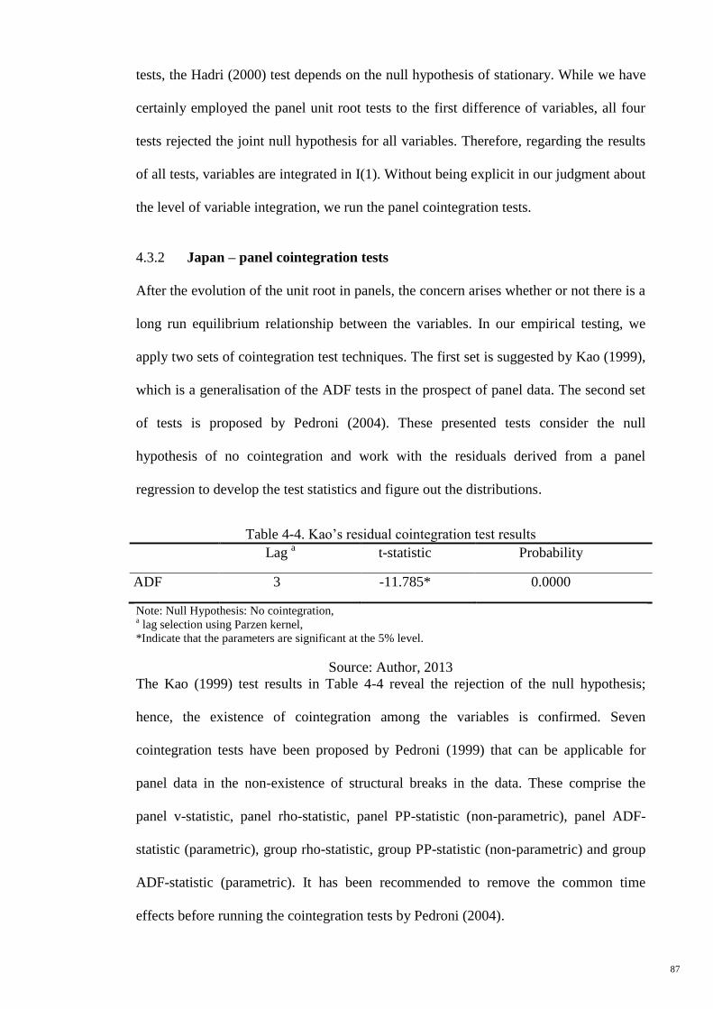
87

tests, the Hadri (2000) test depends on the null hypothesis of stationary. While we have

certainly employed the panel unit root tests to the first difference of variables, all four

tests rejected the joint null hypothesis for all variables. Therefore, regarding the results

of all tests, variables are integrated in I(1). Without being explicit in our judgment about

the level of variable integration, we run the panel cointegration tests.

4.3.2 Japan – panel cointegration tests

After the evolution of the unit root in panels, the concern arises whether or not there is a

long run equilibrium relationship between the variables. In our empirical testing, we

apply two sets of cointegration test techniques. The first set is suggested by Kao (1999),

which is a generalisation of the ADF tests in the prospect of panel data. The second set

of tests is proposed by Pedroni (2004). These presented tests consider the null

hypothesis of no cointegration and work with the residuals derived from a panel

regression to develop the test statistics and figure out the distributions.

Table 4-4. Kao’s residual cointegration test results

Lag a t-statistic Probability

ADF 3 -11.785* 0.0000

Note: Null Hypothesis: No cointegration,

a lag selection using Parzen kernel,

*Indicate that the parameters are significant at the 5% level.


The Kao (1999) test results in Table 4-4 reveal the rejection of the null hypothesis;

hence, the existence of cointegration among the variables is confirmed. Seven

cointegration tests have been proposed by Pedroni (1999) that can be applicable for

panel data in the non-existence of structural breaks in the data. These comprise the

panel v-statistic, panel rho-statistic, panel PP-statistic (non-parametric), panel ADF-

statistic (parametric), group rho-statistic, group PP-statistic (non-parametric) and group

ADF-statistic (parametric). It has been recommended to remove the common time

effects before running the cointegration tests by Pedroni (2004).

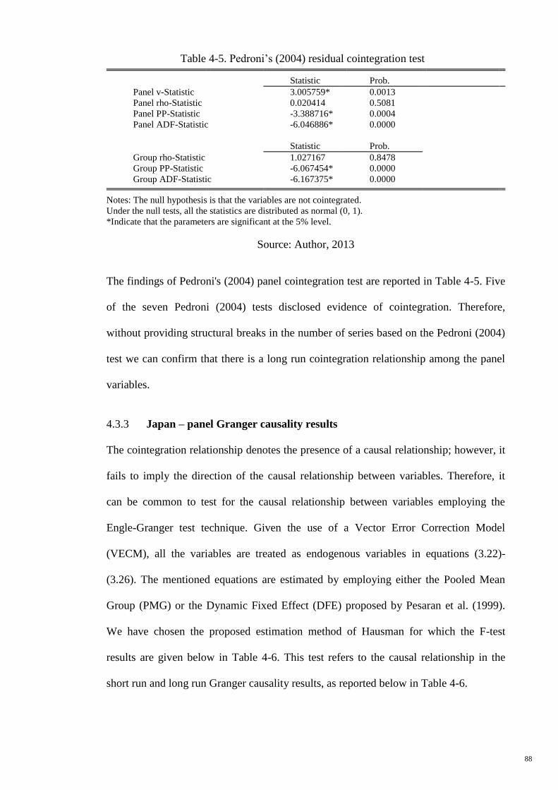
88

Table 4-5. Pedroni’s (2004) residual cointegration test Statistic Prob.

Panel v-Statistic 3.005759* 0.0013

Panel rho-Statistic 0.020414 0.5081

Panel PP-Statistic -3.388716* 0.0004

Panel ADF-Statistic -6.046886* 0.0000

Statistic Prob.

Group rho-Statistic 1.027167 0.8478

Group PP-Statistic -6.067454* 0.0000

Group ADF-Statistic -6.167375* 0.0000

Notes: The null hypothesis is that the variables are not cointegrated.

Under the null tests, all the statistics are distributed as normal (0, 1).



The findings of Pedroni's (2004) panel cointegration test are reported in Table 4-5. Five

of the seven Pedroni (2004) tests disclosed evidence of cointegration. Therefore,

without providing structural breaks in the number of series based on the Pedroni (2004)

test we can confirm that there is a long run cointegration relationship among the panel

variables.

4.3.3 Japan – panel Granger causality results

The cointegration relationship denotes the presence of a causal relationship; however, it

fails to imply the direction of the causal relationship between variables. Therefore, it

can be common to test for the causal relationship between variables employing the

Engle-Granger test technique. Given the use of a Vector Error Correction Model

(VECM), all the variables are treated as endogenous variables in equations (3.22)-

(3.26). The mentioned equations are estimated by employing either the Pooled Mean

Group (PMG) or the Dynamic Fixed Effect (DFE) proposed by Pesaran et al. (1999).

We have chosen the proposed estimation method of Hausman for which the F-test

results are given below in Table 4-6. This test refers to the causal relationship in the

short run and long run Granger causality results, as reported below in Table 4-6.

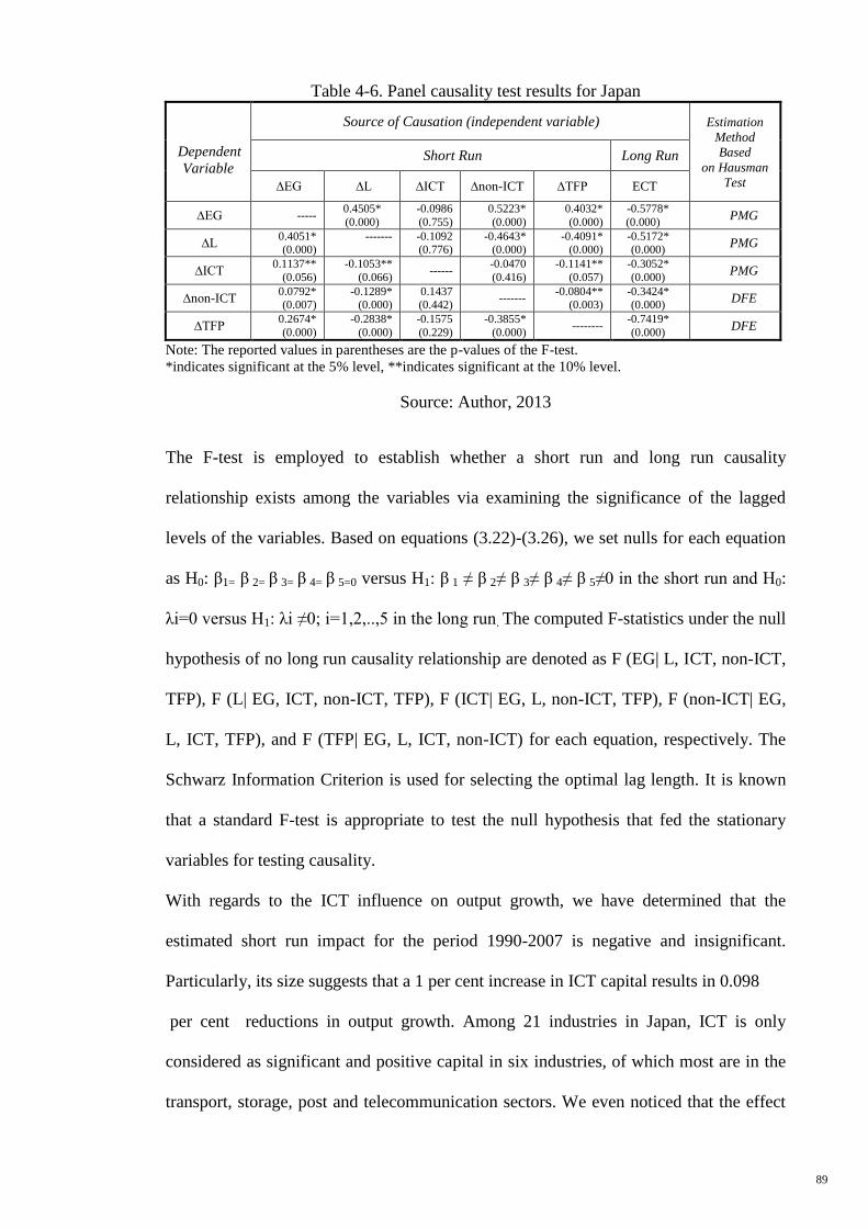
89

Table 4-6. Panel causality test results for Japan

Dependent

Variable

Source of Causation (independent variable) Estimation

Method

Based

on Hausman

Test

Short Run Long Run

∆EG ∆L ∆ICT ∆non-ICT ∆TFP ECT

∆EG ----- 0.4505*

(0.000)

-0.0986

(0.755)

0.5223*

(0.000)

0.4032*

(0.000)

-0.5778*

(0.000) PMG

∆L 0.4051* (0.000)

-------

-0.1092 (0.776)

-0.4643* (0.000)

-0.4091* (0.000)

-0.5172* (0.000)

PMG

∆ICT 0.1137**

(0.056)

-0.1053**

(0.066) ------

-0.0470

(0.416)

-0.1141**

(0.057)

-0.3052*

(0.000) PMG

∆non-ICT 0.0792* (0.007)

-0.1289* (0.000)

0.1437 (0.442)

------- -0.0804**

(0.003) -0.3424* (0.000)

DFE

∆TFP 0.2674*

(0.000)

-0.2838*

(0.000)

-0.1575

(0.229)

-0.3855*

(0.000) --------

-0.7419*

(0.000) DFE

Note: The reported values in parentheses are the p-values of the F-test.

*indicates significant at the 5% level, **indicates significant at the 10% level.


The F-test is employed to establish whether a short run and long run causality

relationship exists among the variables via examining the significance of the lagged

levels of the variables. Based on equations (3.22)-(3.26), we set nulls for each equation

as H0: β1= β 2= β 3= β 4= β 5=0 versus H1: β 1 ≠ β 2≠ β 3≠ β 4≠ β 5≠0 in the short run and H0:

λi=0 versus H1: λi ≠0; i=1,2,..,5 in the long run. The computed F-statistics under the null

hypothesis of no long run causality relationship are denoted as F (EG| L, ICT, non-ICT,

TFP), F (L| EG, ICT, non-ICT, TFP), F (ICT| EG, L, non-ICT, TFP), F (non-ICT| EG,

L, ICT, TFP), and F (TFP| EG, L, ICT, non-ICT) for each equation, respectively. The

Schwarz Information Criterion is used for selecting the optimal lag length. It is known

that a standard F-test is appropriate to test the null hypothesis that fed the stationary

variables for testing causality.

With regards to the ICT influence on output growth, we have determined that the

estimated short run impact for the period 1990-2007 is negative and insignificant.

Particularly, its size suggests that a 1 per cent increase in ICT capital results in 0.098

per cent reductions in output growth. Among 21 industries in Japan, ICT is only

considered as significant and positive capital in six industries, of which most are in the

transport, storage, post and telecommunication sectors. We even noticed that the effect

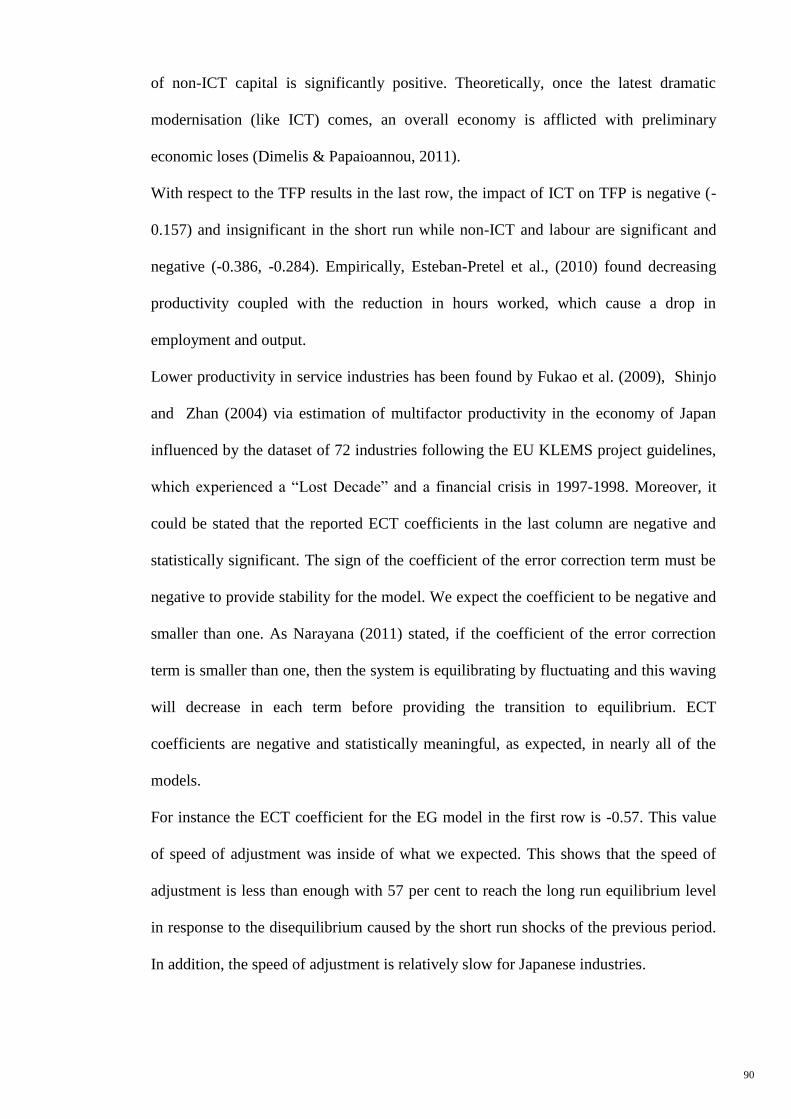
90

of non-ICT capital is significantly positive. Theoretically, once the latest dramatic

modernisation (like ICT) comes, an overall economy is afflicted with preliminary

economic loses (Dimelis & Papaioannou, 2011).

With respect to the TFP results in the last row, the impact of ICT on TFP is negative (-

0.157) and insignificant in the short run while non-ICT and labour are significant and

negative (-0.386, -0.284). Empirically, Esteban-Pretel et al., (2010) found decreasing

productivity coupled with the reduction in hours worked, which cause a drop in

employment and output.

Lower productivity in service industries has been found by Fukao et al. (2009), Shinjo

and Zhan (2004) via estimation of multifactor productivity in the economy of Japan

influenced by the dataset of 72 industries following the EU KLEMS project guidelines,

which experienced a “Lost Decade” and a financial crisis in 1997-1998. Moreover, it

could be stated that the reported ECT coefficients in the last column are negative and

statistically significant. The sign of the coefficient of the error correction term must be

negative to provide stability for the model. We expect the coefficient to be negative and

smaller than one. As Narayana (2011) stated, if the coefficient of the error correction

term is smaller than one, then the system is equilibrating by fluctuating and this waving

will decrease in each term before providing the transition to equilibrium. ECT

coefficients are negative and statistically meaningful, as expected, in nearly all of the

models.

For instance the ECT coefficient for the EG model in the first row is -0.57. This value

of speed of adjustment was inside of what we expected. This shows that the speed of

adjustment is less than enough with 57 per cent to reach the long run equilibrium level

in response to the disequilibrium caused by the short run shocks of the previous period.

In addition, the speed of adjustment is relatively slow for Japanese industries.

91

Table 4-7. Panel industries direction of causality in the short run and long run, Japan




The results in Table 4-7 show the long run bidirectional Granger causality running from

real GDP growth to the contribution of L, ICT, non-ICT, and TFP growth at the per cent

significant level. Except ICT capital, there is a bidirectional Granger causality

relationship among the contribution of L, ICT, non-ICT, and TFP growth to value added

growth in the short run as well. As a result, in line with the findings of Fueki and

Kawamoto (2009), and Miyagawa, Ito, and Harada (2004) at the industrial level, we

found that the increase in overall TFP growth certainly emerges from a rise in

technological change. The findings in Table 4-7 indicate that there is panel short run

bidirectional causality among L, non-ICT and TFP, which means that non-ICT and

labour contribution could be an effective factor on TFP growth in 1990-2007. There is

no causality relationship between ICT and non-ICT capital during the period in the short

run.

We conclude that the short run results for causality are significantly weak; nevertheless,

the long run outcomes are highly significant. The long run results concerning the impact

Short Run causality Long Run causality

Direction of Causality Wald F-test Direction of Causality Wald F-test

∆EG ∆L

(0.000)*

(0.000)* EG -------- L

(0.000)*

(0.000)*

∆EG --------- ∆ICT (0.755)

(0.056)** EG ------ ICT

(0.000)*

(0.000)*

∆EG ∆non-ICT

(0.000)**

(0.007)** EG ------ non-ICT

(0.000)*

(0.000)*

∆EG ∆TFP (0.000)*

(0.000)* EG ------ TFP

(0.000)*

(0.000)*

∆L -------- ∆ICT

(0.776)

(0.066)**

L ------ ICT

(0.000)*

(0.000)*

∆L ∆non-ICT

(0.000)*

(0.000)* L ------ non-ICT

(0.000)*

(0.000)*

∆L ∆TFP

(0.000)*

(0.000)*

L ------ TFP

(0.000)*

(0.000)*

∆ICT no causality ∆non-ICT

(0.416)

(0.442)

ICT ------ non-ICT

(0.000)*

(0.000)*

∆ICT ------- ∆TFP (0.057)**

(0.229)

ICT ------ TFP

(0.000)*

(0.000)*

∆non-ICT∆TFP (0.003)*

(0.000)* non-ICT ------ TFP

(0.000)*

(0.000)*

92

of ICT on GDP growth is inconsistent with those of Elsadig (2010) for a panel of

ASEAN 5 – Malaysia, Indonesia, Philippines, Singapore and Thailand, plus 3 countries

– China, Japan and South Korea (Shimizu, Ogawa, & Fujinuma, 2006).

4.3.4 Japan – long run relationship by System GMM

The GMM estimator, either the system or the first difference version, possesses one and

two-step categories. The two-step estimator is approximately more efficient; but the

standard errors are downwards biased and cause the GMM estimates to be ineffective

for inference (Arellano & Bond, 1991). This issue is mitigated in the System GMM

version since it includes the finite sample correction to the two-step covariance matrix

(Windmeijer, 2005). For this reason, the results of the two-step System GMM

estimators in columns (3) and (4) are more significant and efficient.

Equation (3.2) could be further augmented by qualitative details constructed as binary

variables implying whether an observation originates from an ICT-producing or ICT-

using industry. The reason for the utilisation of such qualitative information might be

derived from Jorgenson and Stiroh (2003), who argued that much of the latest US

growth renaissance occurred in industries producing. Thus, the "electrical and optical

equipment" industry is introduced as an ICT-producing industry in our research.

Extensive ICT-using industries were considered while the coefficient of ICT capital

becomes significant in the PMG estimations results, which are listed as "transport and

storage, communication", "post and telecommunications", "electrical and optical

equipment", manufacturing and recycling", "electricity, gas and water supply", and "

other non-metallic mineral" industries for Japan. Thus, ICT_PROD and ICT_USE,

which are included as binary variables, show that the returns to ICT are higher in ICT-

producing than ICT-using industries.

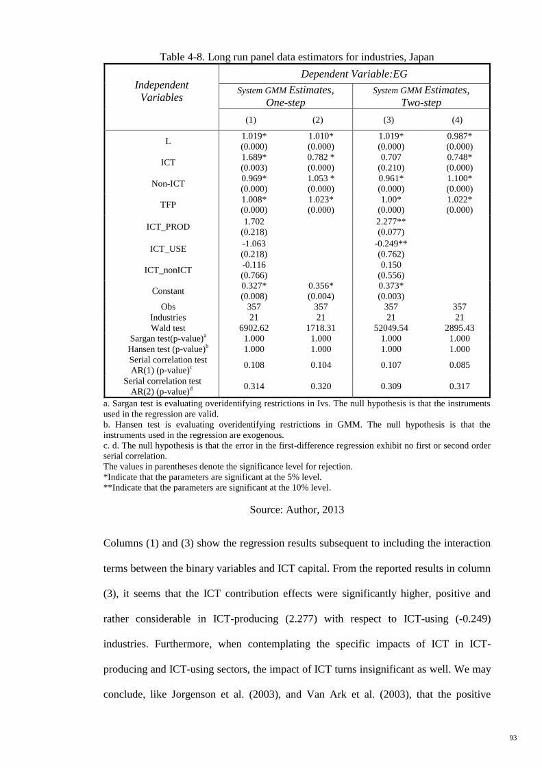
93

Table 4-8. Long run panel data estimators for industries, Japan

Independent

Variables

Dependent Variable:EG

System GMM Estimates,

One-step


Two-step

(1) (2) (3) (4)

L 1.019*

(0.000)

1.010*

(0.000)

1.019*

(0.000)

0.987*

(0.000)

ICT 1.689*

(0.003)

0.782 *

(0.000)

0.707

(0.210)

0.748*

(0.000)

Non-ICT 0.969*

(0.000)

1.053 *

(0.000)

0.961*

(0.000)

1.100*

(0.000)

TFP 1.008*

(0.000)

1.023*

(0.000)

1.00*

(0.000)

1.022*

(0.000)

ICT_PROD 1.702

(0.218)

2.277**

(0.077)

ICT_USE -1.063

(0.218)

-0.249**

(0.762)

ICT_nonICT -0.116

(0.766)

0.150

(0.556)

Constant 0.327*

(0.008)

0.356*

(0.004)

0.373*

(0.003)

Obs 357 357 357 357

Industries 21 21 21 21

Wald test 6902.62 1718.31 52049.54 2895.43

Sargan test(p-value)a 1.000 1.000 1.000 1.000

Hansen test (p-value)b 1.000 1.000 1.000 1.000

Serial correlation test

AR(1) (p-value)c

0.108 0.104 0.107 0.085


AR(2) (p-value)d

0.314 0.320 0.309 0.317

a. Sargan test is evaluating overidentifying restrictions in Ivs. The null hypothesis is that the instruments

used in the regression are valid.

b. Hansen test is evaluating overidentifying restrictions in GMM. The null hypothesis is that the

instruments used in the regression are exogenous.

c. d. The null hypothesis is that the error in the first-difference regression exhibit no first or second order

serial correlation.

The values in parentheses denote the significance level for rejection.


**Indicate that the parameters are significant at the 10% level.


Columns (1) and (3) show the regression results subsequent to including the interaction

terms between the binary variables and ICT capital. From the reported results in column

(3), it seems that the ICT contribution effects were significantly higher, positive and

rather considerable in ICT-producing (2.277) with respect to ICT-using (-0.249)

industries. Furthermore, when contemplating the specific impacts of ICT in ICT-

producing and ICT-using sectors, the impact of ICT turns insignificant as well. We may

conclude, like Jorgenson et al. (2003), and Van Ark et al. (2003), that the positive

94

impact of ICT is mainly centred on ICT intensive industries (Jorgenson et al., 2003).

Moreover, the insignificant ICT coefficient in column (3) shows that the adoption of the

Japan economic system with the diffusion of new ICT was weak and prove that the

contribution of conventional capital like non-ICT and labour to annual economic growth

is more than ICT capital.

In spite of the above, we plan to examine the complementary hypothesis between ICT

and non-ICT capital by inserting in their interaction term (ICT_non-ICT) as an

independent regressor. The results prove that no significant complementary impacts can

be found between ICT and non-ICT capital. On the other hand, the reported findings in

the last column are in line with the PMG short run results of Table 4-6, which shows

that the growth of ICT capital contribution in Japan is less than other capital to value

added growth between 1990 and 2007.

The reported results of the System GMM estimators present two diagnostic tests – the

Sargan and Hansen tests, which check for the validity of normal-type instruments and

GMM-type instruments. The hypothesis examined with the Hansen and Sargan tests is

that the two kinds of instruments are uncorrelated with the residuals, and, therefore, are

appropriate instruments. Our null hypothesis proved that the instruments pass the test

and are regarded as valid by this criterion. This estimator additionally records a test for

the first and second serial correlation, which is employed on the first differenced

residuals. If the null of no autocorrelation is not rejected then the test implies that lags

of the employed instruments have been in fact exogenous and thus are found to be

‘good’ instruments.

4.3.5 Justification of insignificant effects of ICT on TFP and GDP growth in

Japan

As mentioned in the literature, the aggregate and sectoral growth accounting exercises

suggest stronger differences of the ICT effect between the Asia-Pacific and European

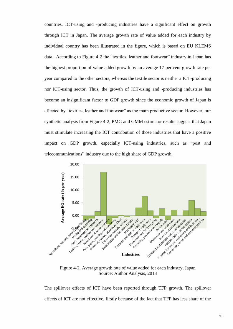
95

countries. ICT-using and -producing industries have a significant effect on growth

through ICT in Japan. The average growth rate of value added for each industry by

individual country has been illustrated in the figure, which is based on EU KLEMS

data. According to Figure 4-2 the “textiles, leather and footwear” industry in Japan has

the highest proportion of value added growth by an average 17 per cent growth rate per

year compared to the other sectors, whereas the textile sector is neither a ICT-producing

nor ICT-using sector. Thus, the growth of ICT-using and -producing industries has

become an insignificant factor to GDP growth since the economic growth of Japan is

affected by “textiles, leather and footwear” as the main productive sector. However, our

synthetic analysis from Figure 4-2, PMG and GMM estimator results suggest that Japan

must stimulate increasing the ICT contribution of those industries that have a positive

impact on GDP growth, especially ICT-using industries, such as “post and

telecommunications” industry due to the high share of GDP growth.

Figure 4-2. Average growth rate of value added for each industry, Japan


The spillover effects of ICT have been reported through TFP growth. The spillover

effects of ICT are not effective, firstly because of the fact that TFP has less share of the

-5.00

0.00

5.00

10.00

15.00

20.00

Av

era

ge

EG

ra

te (

% p

er y

ear)

Industries

96

output growth of Japanese industries, and, secondly, the low number of industries that

are ICT-using. From 21 classified industries, only six have a positive significant effect

of ICT, which are all ICT-using sectors. On the other hand, based on the unidirectional

granger causality running from TFP growth to ICT contribution, there is still a

productivity paradox for the Japanese sectors, which is the consequence of negative

insignificant effects of ICT on TFP. The positive significant effects of TFP on GDP

growth in the long run may not attribute to ICT growth. This can be interpreted as there

being no evidence to prove the absence of spillover effects of ICT for Japanese

industries that leads to a significant effect of ICT on GDP growth. All of these findings

show that ICT does not have a significant effect on value added growth.

The overall proportion of ICT-using industries in Japan, such as "transport, storage and

communication", "post and telecommunications", "electricity, gas and water supply"

from GDP growth are more than other industries; therefore, the output growth rate

would be increased if ICT-using industries have been stimulated to penetrate and

investment in ICT. Therefore one of the suitable policy implications can be to stimulate

penetrating and investing in ICT, such as the “textiles, leather and footwear” industry,

which is capable of increasing GDP growth.

Two decades ago, Japan was acknowledged to be a popular ICT-producer. Nowadays,

Japan's economy is weak in both ICT-producing and using sectors. It seems that a lack

of competition and excessive regulations in the public service sector have hindered the

effects of ICT-usage and also the quest for renewed sustainable growth paths while

lowering the productivity in the service industries. It has been found in this study that

the main reason behind Japan’s lost decade is the slow-down of TFP. Growth in Japan’s

TFP is now believed to be primarily supported by the ICT-using industries. Recently,

Japan is losing its advantages in telecommunication infrastructure and also lagging

behind in availability and utilisation, as shown in Figure 4-3.

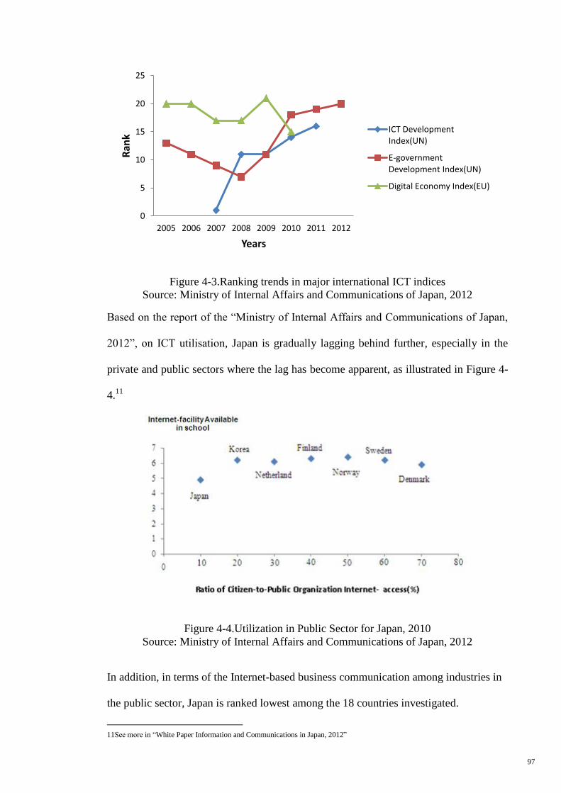
97

Figure 4-3.Ranking trends in major international ICT indices Source: Ministry of Internal Affairs and Communications of Japan, 2012

Based on the report of the “Ministry of Internal Affairs and Communications of Japan,

2012”, on ICT utilisation, Japan is gradually lagging behind further, especially in the

private and public sectors where the lag has become apparent, as illustrated in Figure 4-

4.11

Figure 4-4.Utilization in Public Sector for Japan, 2010

Source: Ministry of Internal Affairs and Communications of Japan, 2012

In addition, in terms of the Internet-based business communication among industries in

the public sector, Japan is ranked lowest among the 18 countries investigated.

11See more in “White Paper Information and Communications in Japan, 2012”

0

5

10

15

20

25

2005 2006 2007 2008 2009 2010 2011 2012

Ran

k

Years

ICT Development Index(UN)

E-government Development Index(UN)

Digital Economy Index(EU)

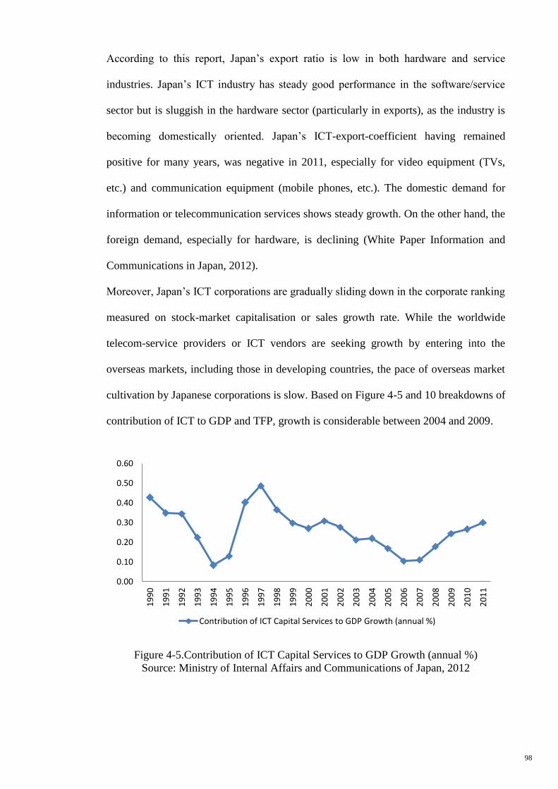
98

According to this report, Japan’s export ratio is low in both hardware and service

industries. Japan’s ICT industry has steady good performance in the software/service

sector but is sluggish in the hardware sector (particularly in exports), as the industry is

becoming domestically oriented. Japan’s ICT-export-coefficient having remained

positive for many years, was negative in 2011, especially for video equipment (TVs,

etc.) and communication equipment (mobile phones, etc.). The domestic demand for

information or telecommunication services shows steady growth. On the other hand, the

foreign demand, especially for hardware, is declining (White Paper Information and

Communications in Japan, 2012).

Moreover, Japan’s ICT corporations are gradually sliding down in the corporate ranking

measured on stock-market capitalisation or sales growth rate. While the worldwide

telecom-service providers or ICT vendors are seeking growth by entering into the

overseas markets, including those in developing countries, the pace of overseas market

cultivation by Japanese corporations is slow. Based on Figure 4-5 and 10 breakdowns of

contribution of ICT to GDP and TFP, growth is considerable between 2004 and 2009.

Figure 4-5.Contribution of ICT Capital Services to GDP Growth (annual %)


0.00

0.10

0.20

0.30

0.40

0.50

0.60

19

90

19

91

19

92

19

93

19

94

19

95

19

96

19

97

19

98

19

99

20

00

20

01

20

02

20

03

20

04

20

05

20

06

20

07

20

08

20

09

20

10

20

11

Contribution of ICT Capital Services to GDP Growth (annual %)

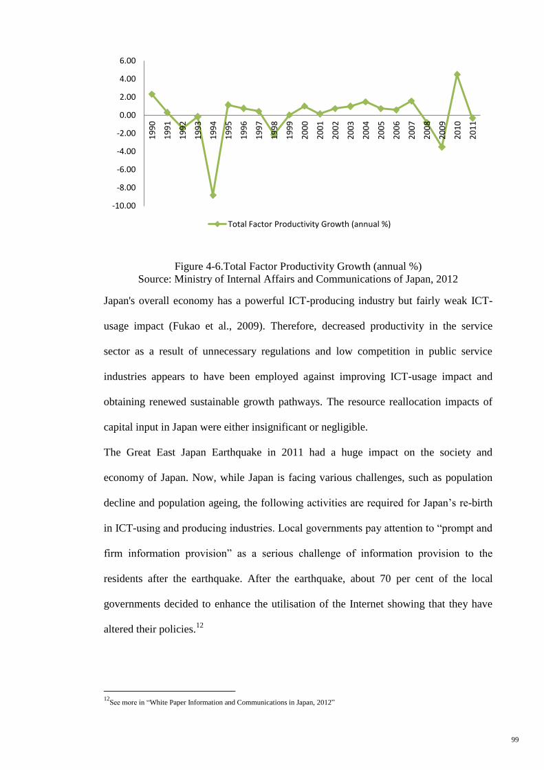
99

Figure 4-6.Total Factor Productivity Growth (annual %)


Japan's overall economy has a powerful ICT-producing industry but fairly weak ICT-

usage impact (Fukao et al., 2009). Therefore, decreased productivity in the service

sector as a result of unnecessary regulations and low competition in public service

industries appears to have been employed against improving ICT-usage impact and

obtaining renewed sustainable growth pathways. The resource reallocation impacts of

capital input in Japan were either insignificant or negligible.

The Great East Japan Earthquake in 2011 had a huge impact on the society and

economy of Japan. Now, while Japan is facing various challenges, such as population

decline and population ageing, the following activities are required for Japan’s re-birth

in ICT-using and producing industries. Local governments pay attention to “prompt and

firm information provision” as a serious challenge of information provision to the

residents after the earthquake. After the earthquake, about 70 per cent of the local

governments decided to enhance the utilisation of the Internet showing that they have

altered their policies.12

12

See more in “White Paper Information and Communications in Japan, 2012”

-10.00

-8.00

-6.00

-4.00

-2.00

0.00

2.00

4.00

6.00

19

90

19

91

19

92

19

93

19

94

19

95

19

96

19

97

19

98

19

99

20

00

20

01

20

02

20

03

20

04

20

05

20

06

20

07

20

08

20

09

20

10

20

11

Total Factor Productivity Growth (annual %)

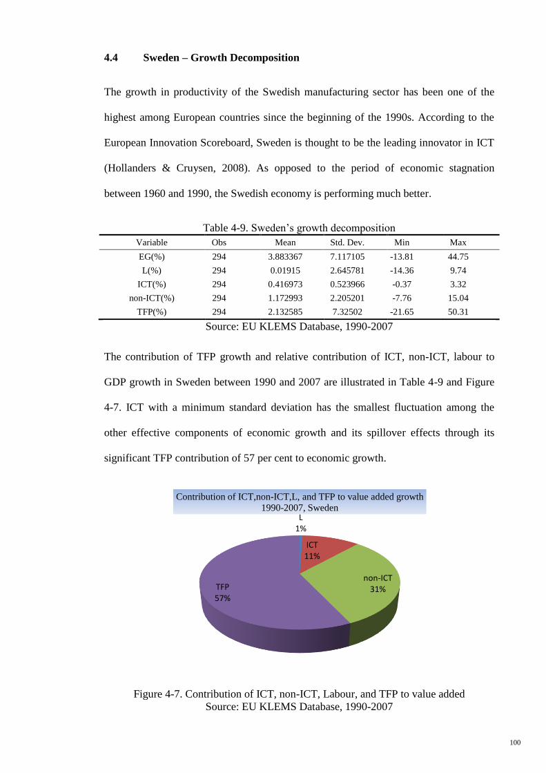
100

4.4 Sweden – Growth Decomposition

The growth in productivity of the Swedish manufacturing sector has been one of the

highest among European countries since the beginning of the 1990s. According to the

European Innovation Scoreboard, Sweden is thought to be the leading innovator in ICT

(Hollanders & Cruysen, 2008). As opposed to the period of economic stagnation

between 1960 and 1990, the Swedish economy is performing much better.

Table 4-9. Sweden’s growth decomposition


EG(%) 294 3.883367 7.117105 -13.81 44.75

L(%) 294 0.01915 2.645781 -14.36 9.74

ICT(%) 294 0.416973 0.523966 -0.37 3.32

non-ICT(%) 294 1.172993 2.205201 -7.76 15.04

TFP(%) 294 2.132585 7.32502 -21.65 50.31


The contribution of TFP growth and relative contribution of ICT, non-ICT, labour to

GDP growth in Sweden between 1990 and 2007 are illustrated in Table 4-9 and Figure

4-7. ICT with a minimum standard deviation has the smallest fluctuation among the

other effective components of economic growth and its spillover effects through its

significant TFP contribution of 57 per cent to economic growth.



L 1%

ICT 11%

non-ICT 31% TFP

57%

Contribution of ICT,non-ICT,L, and TFP to value added growth

1990-2007, Sweden

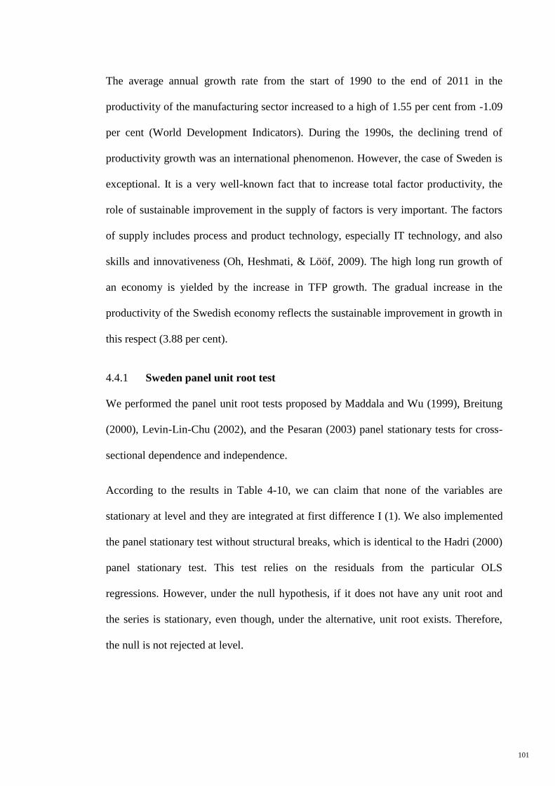
101

The average annual growth rate from the start of 1990 to the end of 2011 in the

productivity of the manufacturing sector increased to a high of 1.55 per cent from -1.09

per cent (World Development Indicators). During the 1990s, the declining trend of

productivity growth was an international phenomenon. However, the case of Sweden is

exceptional. It is a very well-known fact that to increase total factor productivity, the

role of sustainable improvement in the supply of factors is very important. The factors

of supply includes process and product technology, especially IT technology, and also

skills and innovativeness (Oh, Heshmati, & Lööf, 2009). The high long run growth of

an economy is yielded by the increase in TFP growth. The gradual increase in the

productivity of the Swedish economy reflects the sustainable improvement in growth in

this respect (3.88 per cent).

4.4.1 Sweden panel unit root test

We performed the panel unit root tests proposed by Maddala and Wu (1999), Breitung

(2000), Levin-Lin-Chu (2002), and the Pesaran (2003) panel stationary tests for cross-

sectional dependence and independence.

According to the results in Table 4-10, we can claim that none of the variables are

stationary at level and they are integrated at first difference I (1). We also implemented

the panel stationary test without structural breaks, which is identical to the Hadri (2000)

panel stationary test. This test relies on the residuals from the particular OLS

regressions. However, under the null hypothesis, if it does not have any unit root and

the series is stationary, even though, under the alternative, unit root exists. Therefore,

the null is not rejected at level.

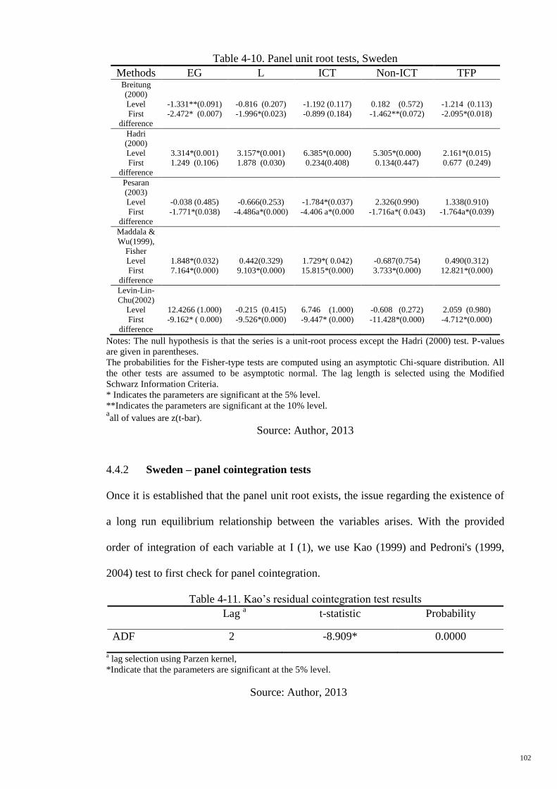
102

Table 4-10. Panel unit root tests, Sweden

Methods EG L ICT Non-ICT TFP Breitung

(2000)

Level

First

difference

-1.331**(0.091)

-2.472* (0.007)

-0.816 (0.207)

-1.996*(0.023)

-1.192 (0.117)

-0.899 (0.184)

0.182 (0.572)

-1.462**(0.072)

-1.214 (0.113)

-2.095*(0.018)

Hadri

(2000)

Level

First

difference

3.314*(0.001)

1.249 (0.106)

3.157*(0.001)

1.878 (0.030)

6.385*(0.000)

0.234(0.408)

5.305*(0.000)

0.134(0.447)

2.161*(0.015)

0.677 (0.249)

Pesaran

(2003)

Level

First

difference

-0.038 (0.485)

-1.771*(0.038)

-0.666(0.253)

-4.486a*(0.000)

-1.784*(0.037)

-4.406 a*(0.000

2.326(0.990)

-1.716a*( 0.043)

1.338(0.910)

-1.764a*(0.039)

Maddala &

Wu(1999),

Fisher

Level

First

difference

1.848*(0.032)

7.164*(0.000)

0.442(0.329)

9.103*(0.000)

1.729*( 0.042)

15.815*(0.000)

-0.687(0.754)

3.733*(0.000)

0.490(0.312)

12.821*(0.000)

Levin-Lin-

Chu(2002)

Level

First

difference

12.4266 (1.000)

-9.162* ( 0.000)

-0.215 (0.415)

-9.526*(0.000)

6.746 (1.000)

-9.447* (0.000)

-0.608 (0.272)

-11.428*(0.000)

2.059 (0.980)

-4.712*(0.000)

Notes: The null hypothesis is that the series is a unit-root process except the Hadri (2000) test. P-values

are given in parentheses.

The probabilities for the Fisher-type tests are computed using an asymptotic Chi-square distribution. All

the other tests are assumed to be asymptotic normal. The lag length is selected using the Modified

Schwarz Information Criteria.


**Indicates the parameters are significant at the 10% level. aall of values are z(t-bar).


4.4.2 Sweden – panel cointegration tests

Once it is established that the panel unit root exists, the issue regarding the existence of

a long run equilibrium relationship between the variables arises. With the provided

order of integration of each variable at I (1), we use Kao (1999) and Pedroni's (1999,

2004) test to first check for panel cointegration.



ADF 2 -8.909* 0.0000




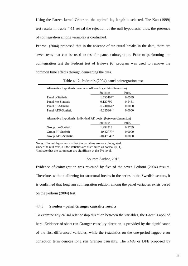
103

Using the Parzen kernel Criterion, the optimal lag length is selected. The Kao (1999)

test results in Table 4-11 reveal the rejection of the null hypothesis; thus, the presence

of cointegration among variables is confirmed.

Pedroni (2004) proposed that in the absence of structural breaks in the data, there are

seven tests that can be used to test for panel cointegration. Prior to performing the

cointegration test the Pedroni test of Eviews (6) program was used to remove the

common time effects through demeaning the data.

Table 4-12. Pedroni's (2004) panel cointegration test

Alternative hypothesis: common AR coefs. (within-dimension)

Statistic Prob.





Alternative hypothesis: individual AR coefs. (between-dimension)

Statistic Prob.

Group rho-Statistic 1.992913 0.9769 Group PP-Statistic -10.42079* 0.0000 Group ADF-Statistic -10.47549* 0.0000





Evidence of cointegration was revealed by five of the seven Pedroni (2004) results.

Therefore, without allowing for structural breaks in the series in the Swedish sectors, it

is confirmed that long run cointegration relation among the panel variables exists based

on the Pedroni (2004) test.

4.4.3 Sweden – panel Granger causality results

To examine any causal relationship direction between the variables, the F-test is applied

here. Evidence of short run Granger causality direction is provided by the significance

of the first differenced variables, while the t-statistics on the one-period lagged error

correction term denotes long run Granger causality. The PMG or DFE proposed by

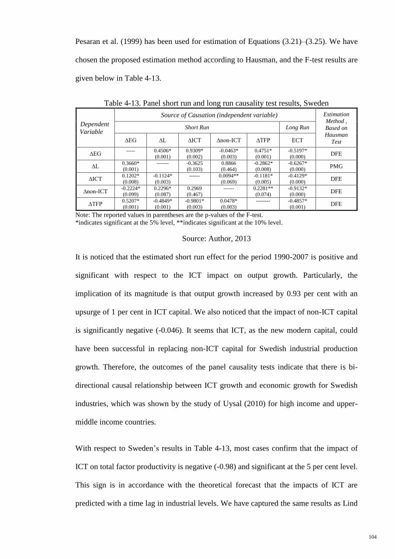
104

Pesaran et al. (1999) has been used for estimation of Equations (3.21)–(3.25). We have

chosen the proposed estimation method according to Hausman, and the F-test results are

given below in Table 4-13.

Table 4-13. Panel short run and long run causality test results, Sweden

Dependent

Variable


Method ,

Based on

Hausman

Test

Short Run Long Run


∆EG ----- 0.4506*

(0.001)

0.9309*

(0.002)

-0.0463*

(0.003)

0.4751*

(0.001)

-0.5197*

(0.000) DFE

∆L 0.3660* (0.001)

-------

-0.3625 (0.103)

0.8866 (0.464)

-0.2862* (0.008)

-0.6267* (0.000)

PMG

∆ICT 0.1202*

(0.008)

-0.1124*

(0.003)

------ 0.0094**

(0.069)

-0.1181*

(0.005)

-0.4129*

(0.000) DFE

∆non-ICT -0.2224* (0.099)

0.2296* (0.087)

0.2969 (0.467)

------ 0.2281** (0.074)

-0.9132* (0.000)

DFE

∆TFP 0.5207*

(0.001)

-0.4849*

(0.001)

-0.9801*

(0.003)

0.0478*

(0.003)

-------- -0.4857*

(0.001) DFE




It is noticed that the estimated short run effect for the period 1990-2007 is positive and

significant with respect to the ICT impact on output growth. Particularly, the

implication of its magnitude is that output growth increased by 0.93 per cent with an

upsurge of 1 per cent in ICT capital. We also noticed that the impact of non-ICT capital

is significantly negative (-0.046). It seems that ICT, as the new modern capital, could

have been successful in replacing non-ICT capital for Swedish industrial production

growth. Therefore, the outcomes of the panel causality tests indicate that there is bi-

directional causal relationship between ICT growth and economic growth for Swedish

industries, which was shown by the study of Uysal (2010) for high income and upper-

middle income countries.

With respect to Sweden’s results in Table 4-13, most cases confirm that the impact of

ICT on total factor productivity is negative (-0.98) and significant at the 5 per cent level.

This sign is in accordance with the theoretical forecast that the impacts of ICT are

predicted with a time lag in industrial levels. We have captured the same results as Lind

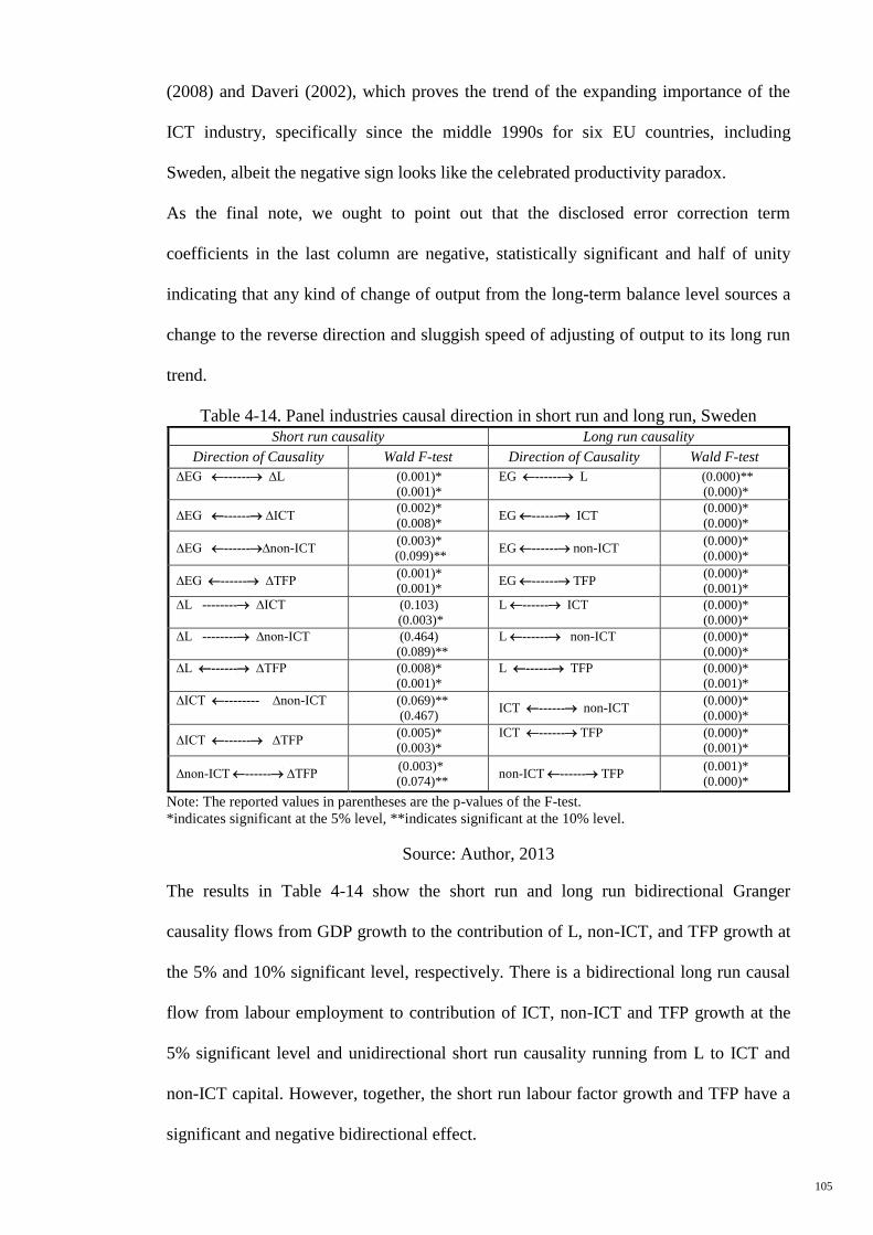
105

(2008) and Daveri (2002), which proves the trend of the expanding importance of the

ICT industry, specifically since the middle 1990s for six EU countries, including

Sweden, albeit the negative sign looks like the celebrated productivity paradox.

As the final note, we ought to point out that the disclosed error correction term

coefficients in the last column are negative, statistically significant and half of unity

indicating that any kind of change of output from the long-term balance level sources a

change to the reverse direction and sluggish speed of adjusting of output to its long run

trend.

Table 4-14. Panel industries causal direction in short run and long run, Sweden




The results in Table 4-14 show the short run and long run bidirectional Granger

causality flows from GDP growth to the contribution of L, non-ICT, and TFP growth at

the 5% and 10% significant level, respectively. There is a bidirectional long run causal

flow from labour employment to contribution of ICT, non-ICT and TFP growth at the

5% significant level and unidirectional short run causality running from L to ICT and

non-ICT capital. However, together, the short run labour factor growth and TFP have a

significant and negative bidirectional effect.

Short run causality Long run causality


∆EG ------ ∆L

(0.001)*

(0.001)*

EG ------ L

(0.000)**

(0.000)*

∆EG ------ ∆ICT (0.002)*

(0.008)* EG ------ ICT

(0.000)*

(0.000)*

∆EG ------∆non-ICT (0.003)*

(0.099)** EG ------ non-ICT

(0.000)*

(0.000)*

∆EG ------ ∆TFP (0.001)*

(0.001)* EG ------ TFP

(0.000)*

(0.001)*

∆L -------- ∆ICT

(0.103)

(0.003)*

L ------ ICT

(0.000)*

(0.000)*

∆L -------- ∆non-ICT

(0.464)

(0.089)**

L ------ non-ICT

(0.000)*

(0.000)*

∆L ------ ∆TFP

(0.008)*

(0.001)*

L ------ TFP

(0.000)*

(0.001)*

∆ICT -------- ∆non-ICT

(0.069)**

(0.467) ICT ------ non-ICT

(0.000)*

(0.000)*

∆ICT ------ ∆TFP (0.005)*

(0.003)*

ICT ------ TFP

(0.000)*

(0.001)*

∆non-ICT ------ ∆TFP (0.003)*

(0.074)** non-ICT ------ TFP

(0.001)*

(0.000)*

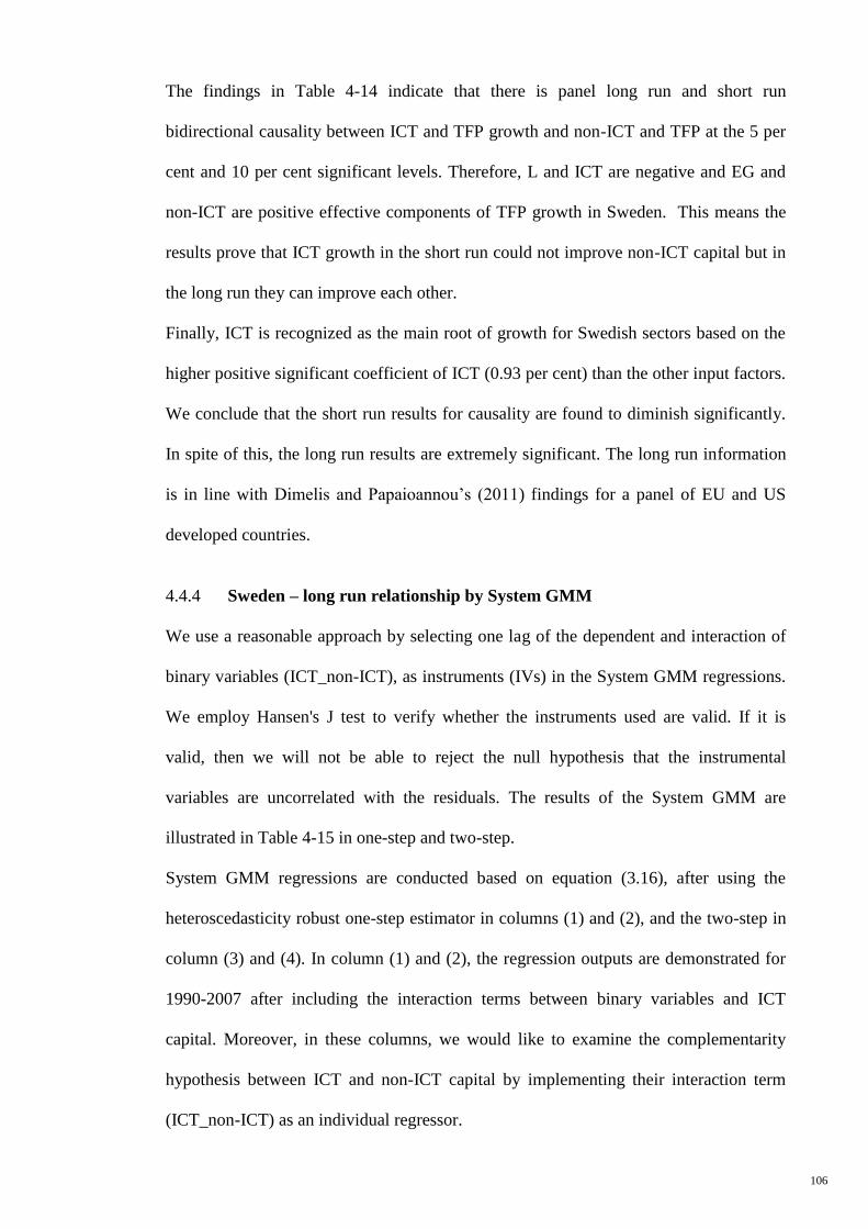
106

The findings in Table 4-14 indicate that there is panel long run and short run

bidirectional causality between ICT and TFP growth and non-ICT and TFP at the 5 per

cent and 10 per cent significant levels. Therefore, L and ICT are negative and EG and

non-ICT are positive effective components of TFP growth in Sweden. This means the

results prove that ICT growth in the short run could not improve non-ICT capital but in

the long run they can improve each other.

Finally, ICT is recognized as the main root of growth for Swedish sectors based on the

higher positive significant coefficient of ICT (0.93 per cent) than the other input factors.

We conclude that the short run results for causality are found to diminish significantly.

In spite of this, the long run results are extremely significant. The long run information

is in line with Dimelis and Papaioannou’s (2011) findings for a panel of EU and US

developed countries.

4.4.4 Sweden – long run relationship by System GMM

We use a reasonable approach by selecting one lag of the dependent and interaction of

binary variables (ICT_non-ICT), as instruments (IVs) in the System GMM regressions.

We employ Hansen's J test to verify whether the instruments used are valid. If it is

valid, then we will not be able to reject the null hypothesis that the instrumental

variables are uncorrelated with the residuals. The results of the System GMM are

illustrated in Table 4-15 in one-step and two-step.

System GMM regressions are conducted based on equation (3.16), after using the

heteroscedasticity robust one-step estimator in columns (1) and (2), and the two-step in

column (3) and (4). In column (1) and (2), the regression outputs are demonstrated for

1990-2007 after including the interaction terms between binary variables and ICT

capital. Moreover, in these columns, we would like to examine the complementarity

hypothesis between ICT and non-ICT capital by implementing their interaction term

(ICT_non-ICT) as an individual regressor.

107

Table 4-15. Long run panel data estimators for industries, Sweden

Independent

Variables

Dependent variable: EG

SystemGMM Estimates,

One-step


Two-step

(1) (2) (3) (4)

L 0.870*

(0.000)

0.899*

(0.000)

0.873*

(0.000)

0.897*

(0.000)

ICT 3.013*

(0.000)

1.405*

(0.005)

3.565*

(0.000)

1.472*

(0.000)

Non-ICT 0.743*

(0.009)

0.364

(0.160)

0.853*

(0.000)

0.350*

(0.000)

TFP 0.957*

(0.000)

0.935*

(0.000)

0.963*

(0.000)

0.931*

(0.000)

ICT_PROD 0.715

(0.459)

0.583

(0.324)

ICT_USE -0.789

(0.269)

-1.229**

(0.091)

ICT_nonICT -0.433*

(0.001)

-0.495*

(0.000)

Constant 0.294**

(0.082)

0.860*

(0.001)

0.149

(0.335)

0.819*

(0.000)

Obs 294 294 294 294


Wald test 15635.21 938.94 83141.30 58612.03

Sargan test

(p-value)a 0.000 0.000 0.000 0.000

Hansen test

(p-value)b 1.000 1.000 1.000 1.000


AR(2) (p-value)c 0.106 0.666 0.206 0.944


AR(3) (p-value)d 0.134 0.099 0.224 0.169






serial correlation.





From the revealed estimations of Table 4-15 it appears evident that the effect of

employment, ICT, and non-ICT capitals on the Sweden industrial growth was extremely

positive and significant during the 17 years, whereas TFP might make a positive and

significant contribution (0.963 per cent) to output growth.

It is clear from the PMG estimators finding, that the overall ICT growth contribution is

positive and significant. Therefore, our estimated results from PMG and GMM have

108

jointly proved that ICT is the main reason of growth of Swedish industries during the

period due to the considerable differences in the ICT coefficient to others.

However, the System GMM results have supplemented these positive effects, which

are more rooted in ICT-using'industries because the effects of ICT-producing industries

are insignificant to value added growth. ICT-producing industries is introduced as

similar to Japan whereas, “food, beverages and tobacco”, ”textiles, leather and

footwear”, “wood and of wood and cork”, “chemical, rubber, plastics and fuel”, “basic

metals and fabricated metal”, “electricity, gas and water supply”, “transport and storage

and communication”, “post and telecommunications”, “finance, insurance, real estate

and business services” and “community social and personal services” industries are

introduced as ICT-using sectors. The results of columns (1) and (3) show that

considerable negative complementary impacts can be found between ICT and non-ICT

capital (interaction term ICT_non-ICT).

On the other hand, the record leads to these columns indicate that the productivity

effects of ICT are significantly bigger in the ICT-using industries. Coupled with the

outcomes of previous tables, we can confirm that the beneficial impacts of ICT are

mainly concentrated in the degree of penetration of ICT between industries, such as the

research results of Jorgenson et al. (2003); Oh, Heshmati, and Lööf (2009b), Van Ark

and Piatkowski (2004).

4.4.5 Justification of significant effects of ICT on TFP and GDP growth in

Sweden

Based on the high GDP share of the ICT-producing sector (20.41 per cent), which is

"Electrical and optical equipment” industries, as illustrated in Figure 4-8, the significant

effects of ICT on TFP and value added growth can be explained. In Sweden, there was

around a twelve-fold decrease in the contribution of “Electrical and optical equipment”

from 24.53 to 2.48 percentage points between 1990 and 2007. However, the average

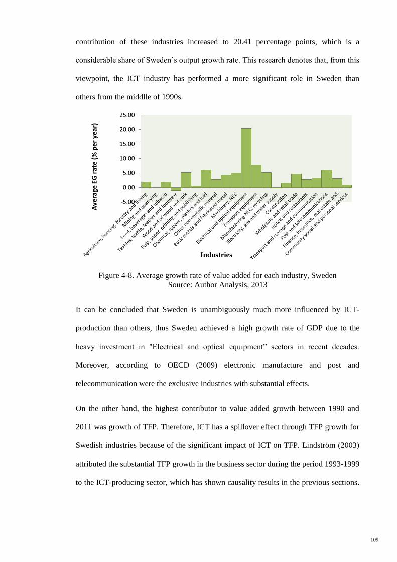
109

contribution of these industries increased to 20.41 percentage points, which is a

considerable share of Sweden’s output growth rate. This research denotes that, from this

viewpoint, the ICT industry has performed a more significant role in Sweden than

others from the middlle of 1990s.

Figure 4-8. Average growth rate of value added for each industry, Sweden


It can be concluded that Sweden is unambiguously much more influenced by ICT-

production than others, thus Sweden achieved a high growth rate of GDP due to the

heavy investment in "Electrical and optical equipment” sectors in recent decades.

Moreover, according to OECD (2009) electronic manufacture and post and

telecommunication were the exclusive industries with substantial effects.

On the other hand, the highest contributor to value added growth between 1990 and

2011 was growth of TFP. Therefore, ICT has a spillover effect through TFP growth for

Swedish industries because of the significant impact of ICT on TFP. Lindström (2003)

attributed the substantial TFP growth in the business sector during the period 1993-1999

to the ICT-producing sector, which has shown causality results in the previous sections.

-5.00

0.00

5.00

10.00

15.00

20.00

25.00

Ave

rage

EG

rat

e (

% p

er y

ear)

Industries

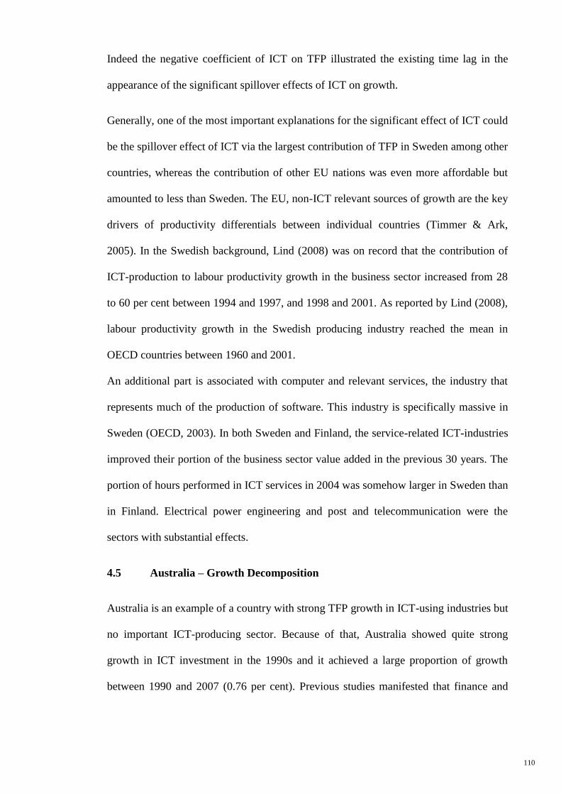
110

Indeed the negative coefficient of ICT on TFP illustrated the existing time lag in the

appearance of the significant spillover effects of ICT on growth.

Generally, one of the most important explanations for the significant effect of ICT could

be the spillover effect of ICT via the largest contribution of TFP in Sweden among other

countries, whereas the contribution of other EU nations was even more affordable but

amounted to less than Sweden. The EU, non-ICT relevant sources of growth are the key

drivers of productivity differentials between individual countries (Timmer & Ark,

2005). In the Swedish background, Lind (2008) was on record that the contribution of

ICT-production to labour productivity growth in the business sector increased from 28

to 60 per cent between 1994 and 1997, and 1998 and 2001. As reported by Lind (2008),

labour productivity growth in the Swedish producing industry reached the mean in

OECD countries between 1960 and 2001.

An additional part is associated with computer and relevant services, the industry that

represents much of the production of software. This industry is specifically massive in

Sweden (OECD, 2003). In both Sweden and Finland, the service-related ICT-industries

improved their portion of the business sector value added in the previous 30 years. The

portion of hours performed in ICT services in 2004 was somehow larger in Sweden than

in Finland. Electrical power engineering and post and telecommunication were the

sectors with substantial effects.

4.5 Australia – Growth Decomposition

Australia is an example of a country with strong TFP growth in ICT-using industries but

no important ICT-producing sector. Because of that, Australia showed quite strong

growth in ICT investment in the 1990s and it achieved a large proportion of growth

between 1990 and 2007 (0.76 per cent). Previous studies manifested that finance and

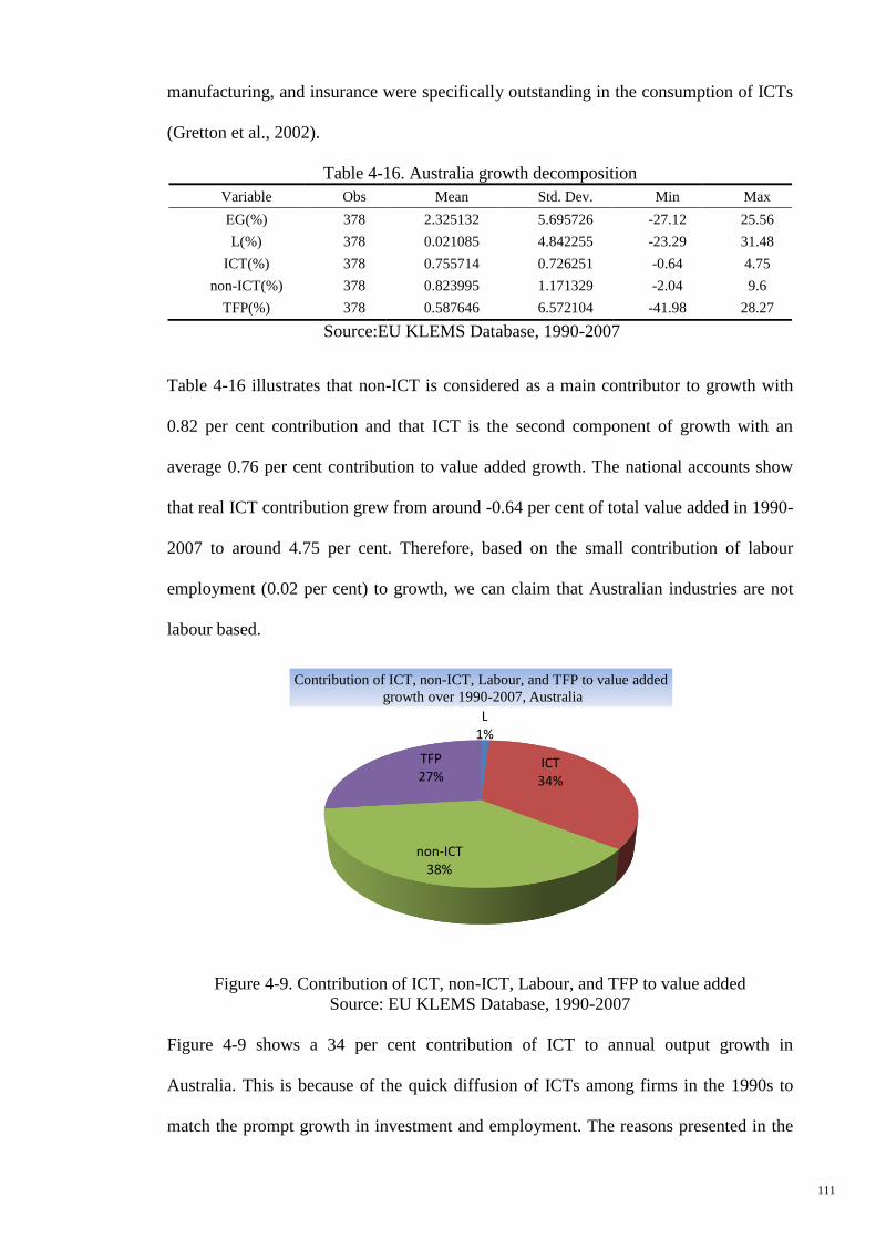
111

manufacturing, and insurance were specifically outstanding in the consumption of ICTs

(Gretton et al., 2002).

Table 4-16. Australia growth decomposition


EG(%) 378 2.325132 5.695726 -27.12 25.56

L(%) 378 0.021085 4.842255 -23.29 31.48

ICT(%) 378 0.755714 0.726251 -0.64 4.75

non-ICT(%) 378 0.823995 1.171329 -2.04 9.6

TFP(%) 378 0.587646 6.572104 -41.98 28.27

Source:EU KLEMS Database, 1990-2007

Table 4-16 illustrates that non-ICT is considered as a main contributor to growth with

0.82 per cent contribution and that ICT is the second component of growth with an

average 0.76 per cent contribution to value added growth. The national accounts show

that real ICT contribution grew from around -0.64 per cent of total value added in 1990-

2007 to around 4.75 per cent. Therefore, based on the small contribution of labour

employment (0.02 per cent) to growth, we can claim that Australian industries are not

labour based.



Figure 4-9 shows a 34 per cent contribution of ICT to annual output growth in

Australia. This is because of the quick diffusion of ICTs among firms in the 1990s to

match the prompt growth in investment and employment. The reasons presented in the

L 1%

ICT 34%

non-ICT 38%

TFP 27%

Contribution of ICT, non-ICT, Labour, and TFP to value added

growth over 1990-2007, Australia

112

literature include that, in 1993-94, around fifty per cent of companies in a great number

of sectors applied computers and around thirty per cent had Internet accessibility. By

2000-05, these proportions grew to nearly eighty-five and seventy per cent respectively

(Gretton et al., 2002). At that time, Australia experienced a 0.27 per cent rise in TFP by

the ICT spillover effect through wide ICT diffusion.

4.5.1 Australia – panel unit root tests

Australia’s outputs of the panel unit root tests are shown in Table 4-17. The test

statistics for the levels of variables are statistically insignificant besides the Levin-Lin-

Chu (2002) test for TFP contribution. Considered as a whole, the results reported that

all five variables are panel non-stationary. When we implement the panel unit root tests

to the first difference of the five variables, almost all tests reject the null hypothesis for

all the variables excluding the Hadri (2000) test, since, within this test, the null is

checked and the panels are stationary.

Table 4-17. Panel unit root tests, Australia

Method EG L ICT Non-ICT TFP

Breitung(2000)

Level

First difference

-0.697(0.243)

2.068*( 0.019)

-0.912(0.181)

-1.508**(0.066)

-0.946(0.172)

-3.866*(0.000)

-1.179(0.119)

-3.113*(0.001)

-1.117(0.132)

-2.453*(0.007)

Hadri(2000)

Level

First difference

2.117*(0.017)

-0.483(0.685)

3.719*(0.000)

0.428(0.335)

6.786*(0.000)

-1.843(0.967)

5.750*(0.000)

-0.518 (0.698)

1.604**(0.054)

-0.923(0.822)

Pesaran (2003)

Level

First difference

1.186a(0.882)

-1.815 a**( 0.035)

2.645a(0.996)

-1.598a* (0.055)

0.033 a( 0.513)

-3.338a*(0.000)

-0.735a(0.231)

-6.305a*( 0.000

-0.315 a(0.376)

-3.813 a*(0.000)

Maddala &

Wu(1999),Fisher

Level

First difference

-1.360(0.913)

5.153*(0.000)

-0.849(0.802)

4.335(0.000)

0.165(0.434)

4.202*(0.000)

-0.254(0.600)

4.958*(0.000)

-0.4069(0.658)

6.395*(0.000)

Levin-Lin-

Chu(2002)

Level

First difference

-1.002(0.158)

-4.479*( 0.000)

0.672(0.749)

-4.977*(0.000)

1.009(0.844)

-6.109*(0.000)

0.715(0.762)

-6.021*(0.000)

-2.009**(0.022)

11.986*(0.000)

Notes: The null hypothesis is that the series is a unit-root process except the Hadri (2000) test. P-values

are given in parentheses.

Probabilities for the Fisher-type tests are computed using an asymptotic Chi-square distribution. All the

other tests are assumed to be asymptotic normal. The lag length is selected using the Modified Schwarz

Information Criteria.




113

A large scale Monte Carlo simulation study by Hlouskova and Wagner (2006)

discovered that the Breitung (2000) panel unit root test usually achieved the highest

strength and the smallest dimension distortions compared to the other panel unit root

tests. Therefore, in general, it can be assumed to determine that all the variables consist

of a panel unit root.

4.5.2 Australia – panel cointegration tests

As it has been established that a unit root exists in all five variables, we proceed by

testing as to whether there is an existence of a long run relationship between EG, L,

ICT, non-ICT, and TFP using the Kao (1999) and Pedroni (2004) heterogeneous panel

cointegration test. Under the assumption of alternative dependent variables, the results

are reported in Tables 4-18 and 4-19.



ADF 3 -12.45962* 0.0000





By using the Parzen Kernel Criterion, the optimal lag length is selected. Kao’s (1999)

test results in Table 4-19 rejected the null hypothesis; thus, the existence of

cointegration among the variables is confirmed.

Monte Carlo simulations using the finite sample distribution for the seven statistics are

tabulated in Pedroni (2004). If the critical values in Pedroni (2004) are exceeded by the

test statistic, then no cointegration null hypothesis is rejected, which implies that a long

run relationship exists between variables.

114

Table 4-19. Pedroni's (2004) panel cointegration test Alternative hypothesis: common AR coefs. (within-dimension)

Statistic Prob.


Panel rho-Statistic -1.029702 0.1516




Statistic Prob.








There are four panel cointegration tests (between dimensions) among the suggested

seven tests by Pedroni (1999) while the others comprise of mean panel cointegration

tests (between dimensions), which are quite general in nature as they allow

heterogeneous coefficients. When the Pedroni (2004) test statistics have a large negative

value, the null hypothesis of no cointegration is rejected by the Pedroni (2004) test

except for the group rho-Statistic, which does not reject the null of no cointegration

when it has a large positive value.

4.5.3 Australia – panel Granger causality results

To demonstrate the existence of a long run relationship between output growth, labour,

ICT, non-ICT and TFP contribution, as shown in Table 4-20, we analyse the direction

of causality between the variables in a panel framework. We designate a model with a

dynamic error correction representation.

The Granger causality test is based on the regressions (3.21) - (3.25) in Chapter 3. ∆

denotes the first difference of the variable and the significance coefficient reveals the

short run causality while the coefficient of the Error Correction Terms (ECT) shows the

long run causality. The optimum lag size was preferred, automatically choosing the

Schwarz information criteria.

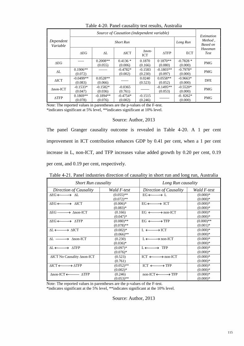
115

Table 4-20. Panel causality test results, Australia

Dependent

Variable


Method ,

Based on

Hausman

Test

Short Run Long Run

∆EG ∆L ∆ICT ∆non-

ICT ∆TFP ECT

∆EG ----- 0.2008**

(0.055)

0.4136 *

(0.006)

0.1870

(0.166)

0 1870**

(0.080)

-0.7828 *

(0.000) PMG

∆L 0.1906**

(0.072)

-------

-0.4782*

(0.002)

-0.1583

(0.230)

-0.1803**

(0.097)

-0.7978*

(0.000) PMG

∆ICT -0.0499**

(0.083)

0.0528**

(0.066) ------

0.0240

(0.523)

0.0558**

(0.052)

-0.9663*

(0.000) DFE

∆non-ICT -0.1533*

(0.047)

-0.1582*

(0.036)

-0.0365

(0.761) -------

-0.1495**

(0.053)

-0.5520*

(0.000) PMG

∆TFP 0.1869**

(0.078)

-0.1894**

(0.076)

-0.4754*

(0.002)

-0.1515

(0.246) --------

-0. 8262*

(0.000) PMG


*indicates significant at 5% level, **indicates significant at 10% level.


The panel Granger causality outcome is revealed in Table 4-20. A 1 per cent

improvement in ICT contribution enhances GDP by 0.41 per cent, when a 1 per cent

increase in L, non-ICT, and TFP increases value added growth by 0.20 per cent, 0.19

per cent, and 0.19 per cent, respectively.

Table 4-21. Panel industries direction of causality in short run and long run, Australia




Short Run causality Long Run causality

Direction of Causality Wald F-test Direction of Causality Wald F-test ∆EG ------ ∆L (0.055)**

(0.072)** EG ------ L (0.000)*

(0.000)*

∆EG ------ ∆ICT (0.006)*

(0.083)*

EG ------ ICT (0.000)*

(0.000)*

∆EG -------- ∆non-ICT (0.166)

(0.047)* EG ------ non-ICT (0.000)*

(0.000)*

∆EG ------ ∆TFP

(0.080)**

(0.078)**

EG ------ TFP (0.000)**

(0.001)*

∆L ------ ∆ICT

(0.002)*

(0.066)**

L ------ ICT

(0.000)*

(0.000)*

∆L -------- ∆non-ICT

(0.230)

(0.036)*

L ------ non-ICT

(0.000)*

(0.000)*

∆L ------ ∆TFP

(0.097)*

(0.076)*

L ------ TFP

(0.000)*

(0.000)*

∆ICT No Causality ∆non-ICT

(0.523)

(0.761)

ICT ------ non-ICT

(0.000)*

(0.000)*

∆ICT ------ ∆TFP (0.052)**

(0.002)* ICT ------ TFP (0.000)*

(0.000)*

∆non-ICT -------- ∆TFP (0.246)

(0.053)** non-ICT ------ TFP (0.000)*

(0.000)*

116

The important point here is that non-ICT capital has become insignificant to GDP

growth in the short run whereas ICT has the most significant positive effect on output

growth similar to the results for Sweden. The findings in Table 4-21 indicate that there

is unidirectional short run panel Granger causality running from EG, labour capital and

TFP to non-ICT. This means that non-ICT in Australia might not be the determining

factor of output and TFP growth in the short run. There is a bidirectional long run

Granger causality between value added growth and the contribution of ICT, non-ICT, L,

and TFP pairwise. Therefore, we can identify ICT as the major source of growth in the

Australian sectors over 1990-2007 (0. 41 per cent). Furthermore, ICT is associated

negatively and significantly to TFP in the long run and also the short run. Therefore, we

can conclude that the evidence is in line with the theoretical expectation that the impacts

of ICT on TFP are expected with a time lag in industrial level to significant effects of

ICT on TFP in the long run. Importantly, these results are in line with the firm level

econometric analysis of Gretton et al. (2004), which controls for other effects and shows

positive connections between ICT use and productivity growth in Australian industries.

However, this result is in contrast to the findings of Colecchia and Schreyer (2002)

about the increasing contribution of ICT to productivity during the second half of the

1990s.

4.5.4 Australia – long run relationship by System GMM

To estimate equation (15), System GMM is applied, which controls the problem of

endogeneity and the serial correlation of regressors. In Table 4-22 below, the estimated

results are specified. Regarding the Australian industries, the System GMM estimates

show that at the 5 per cent significant level (0.98 per cent, 0.95 per cent) the output

elasticities of labour and ICT capital are significant and highly positive. Overall, there is

a positive and significant ICT growth contribution in both the one-step and two-step

results (columns 1 and 3). These results are in line with the long run PMG estimators

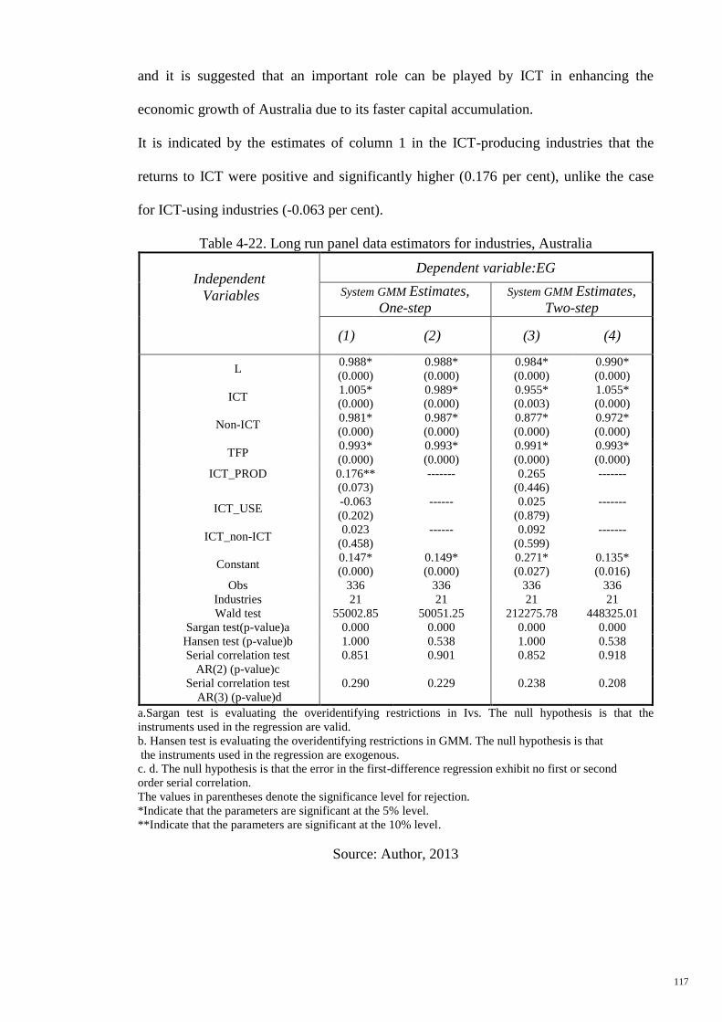
117

and it is suggested that an important role can be played by ICT in enhancing the

economic growth of Australia due to its faster capital accumulation.

It is indicated by the estimates of column 1 in the ICT-producing industries that the

returns to ICT were positive and significantly higher (0.176 per cent), unlike the case

for ICT-using industries (-0.063 per cent).

Table 4-22. Long run panel data estimators for industries, Australia

Independent

Variables

Dependent variable:EG


One-step


Two-step

(1) (2) (3) (4)

L 0.988*

(0.000)

0.988*

(0.000)

0.984*

(0.000)

0.990*

(0.000)

ICT 1.005*

(0.000)

0.989*

(0.000)

0.955*

(0.003)

1.055*

(0.000)

Non-ICT 0.981*

(0.000)

0.987*

(0.000)

0.877*

(0.000)

0.972*

(0.000)

TFP 0.993*

(0.000)

0.993*

(0.000)

0.991*

(0.000)

0.993*

(0.000)

ICT_PROD

0.176**

(0.073)

------- 0.265

(0.446)

-------

ICT_USE -0.063

(0.202)

------ 0.025

(0.879)

-------

ICT_non-ICT 0.023

(0.458)

------ 0.092

(0.599)

-------

Constant 0.147*

(0.000)

0.149*

(0.000)

0.271*

(0.027)

0.135*

(0.016)

Obs 336 336 336 336


Wald test 55002.85 50051.25 212275.78 448325.01




AR(2) (p-value)c

0.851 0.901 0.852 0.918


AR(3) (p-value)d

0.290 0.229 0.238 0.208

a.Sargan test is evaluating the overidentifying restrictions in Ivs. The null hypothesis is that the

instruments used in the regression are valid.

b. Hansen test is evaluating the overidentifying restrictions in GMM. The null hypothesis is that

the instruments used in the regression are exogenous.

c. d. The null hypothesis is that the error in the first-difference regression exhibit no first or second

order serial correlation.





118

The evidence found is in line with the study of O’Mahony (2005) and Van Ark et al.

(2003) who argued that there is still a solid prospective in the EU service industries that

make intensive use of ICT to exploit growth benefits. Therefore, the Australian

economy can capture a higher contribution of ICT and growth in GDP through the

reinforcement of intensive ICT-using industries.

Furthermore, based on the results in column 3, neither ICT-producing nor ICT-using

industries have an insignificant effect on growth. Specifically, the estimates derived

give an indication that the contribution of ICT was 0.27 per cent more in ICT-producing

and 0.03% more in ICT-using industries relative to the remaining industries. The impact

of ICT on growth in ICT-using and producing industries was quite sizable and

significantly higher (interaction terms of ICT_PROD and ICT_USE, respectively), as

per the results reported in the third column of Table 4-22. The evidence in line with this

discussion, that the productivity advantage of the Australian economy has been linked

to the sectors that are either heavy users of ICT or producers of ICT, is quite substantial.

Moreover, it appears that compared to the ICT-using industries, higher returns are

enjoyed by ICT-producing industries. Thus, ICT-producing industries have significantly

higher productivity effects of ICT. In combination with the previous discussion results,

it can be concluded that the beneficial effects of ICTs are mostly focussed on ICT

intensive industries (Draca, Sadun, & Reenen, 2006; Pilat, 2004; Shao & Shu, 2004).

The Hansen test accepts the null hypothesis, which states the validity of the instruments

used in the regressions. Moreover, the null hypothesis is accepted by the test that

examines the second and third-order serial correlation, which means that there is no

evidence of second and third-order serial correlation in the error term. Additional

support is granted to the estimates reported in Table 4-22 by the results of both tests.

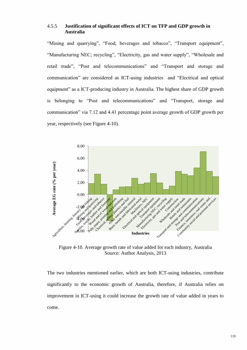
119

4.5.5 Justification of significant effects of ICT on TFP and GDP growth in

Australia

“Mining and quarrying”, “Food, beverages and tobacco”, “Transport equipment”,

“Manufacturing NEC; recycling”, “Electricity, gas and water supply”, “Wholesale and

retail trade”, “Post and telecommunications” and “Transport and storage and

communication” are considered as ICT-using industries and “Electrical and optical

equipment” as a ICT-producing industry in Australia. The highest share of GDP growth

is belonging to “Post and telecommunications” and “Transport, storage and

communication” via 7.12 and 4.41 percentage point average growth of GDP growth per

year, respectively (see Figure 4-10).

Figure 4-10. Average growth rate of value added for each industry, Australia


The two industries mentioned earlier, which are both ICT-using industries, contribute

significantly to the economic growth of Australia, therefore, if Australia relies on

improvement in ICT-using it could increase the growth rate of value added in years to

come.

-6.00

-4.00

-2.00

0.00

2.00

4.00

6.00

8.00

Av

era

ge

EG

ra

te (

% p

er y

ear)

Industries

120

Australia, with an average 3.47 per cent share of ICT-producing sector from GDP

growth has the smallest portion of ICT-producing industries among five countries. The

largest ICT manufacturing sectors are Ireland and Finland, trailed by Korea. In contrast,

Australia and New Zealand only have a small sector, which produces manufactured ICT

goods (Margaret & Ray, 2003). According to this study, for the period under

consideration, for the countries to benefit from effects of ICT on growth, the lack of a

large ICT-producing industry is not necessarily an impediment. Australia is a prime

example in that although it only has a small ICT-producing sector it has significantly

benefited from ICT capital services.

ICT and non-ICT capital with 38 per cent and 34 per cent, respectively, are the highest

contributors to value added growth over 1990-2011 in Australia. However, from the

large magnitude coefficient of ICT in comparison to non-ICT in the GMM results, ICT

could be a kind of economic growth source in Australia via the high penetration of ICT.

Furthermore, one of the reasons for the high penetration of ICT in Australia is from the

establishment of an organisation called Australia's Information and Communications

Technology Research Centre of Excellence (NICTA) in 2002, which was built to

strengthen investment and build capacity in communications technology and strategic

information research. There could be an improvement in the ability of Australia to fully

capture the transformational and productivity benefits brought forth by the

communication and information technology.

“NICTA” will help in the transformation of the ICT sector of Australia and the

traditionally strong competitiveness of the sector will be strengthened, such as primary

industries, entertainment, financial services, health, education and resources. NICTA is

an independent company, which is a not-for-profit and is limited by guarantee.

Its four founding member organisations are the "ACT Government", “Australian

National University", "University of New South Wales", and “NSW Government". The



121

ICT effect on GDP over 1990-2001 was 0.99, which changed to 1.06 during 2001-2011;

therefore the performance of the NICTA organization is considerable in stimulating the

penetration of ICT after 2002 (OECD, 2002).

The spillover effects of ICT with time lagging through increasing TFP have stimulated

the direct significant effects of ICT on growth. On the other hand, the contribution of

ICT capital to GDP growth was the largest in Australia, which is 0.75 per cent on

average over the years 1990-2011; followed by Finland among the other five countries

in this research.

4.6 Finland – Growth Decomposition

Recently, in terms of GDP growth and labour productivity contribution, the leading

industry in Finland is the communication and information technology sector. Labour

productivity in Finland, which is measured by means of the value added per hour

worked in four manufacturing industries – basic metals, telecommunications equipment,

pulp and paper, and wood and wood products – is the highest relative to the other EU-

15 member countries in 2001.

Real gross valued added measures the output while over the entire period, 90% of

output growth arises from growth in TFP, particularly labour productivity. In the two

decades, relative contribution of TFP was at its highest in Finland. As many industrial

nations have suffered slowdown in the productivity recently, Finland has done better

inasmuch as it has not been affected by a productivity slowdown to the same extent as

other nations. This is mainly down to its success as an ICT-producer.

In the early 1990s, severe depression hit the Finnish economy. In the non-residential

market sector, there was a 10 per cent fall in the volume of gross value between 1990

and 1992. However, the recovery was quick, and, by the looks of it, there was no major

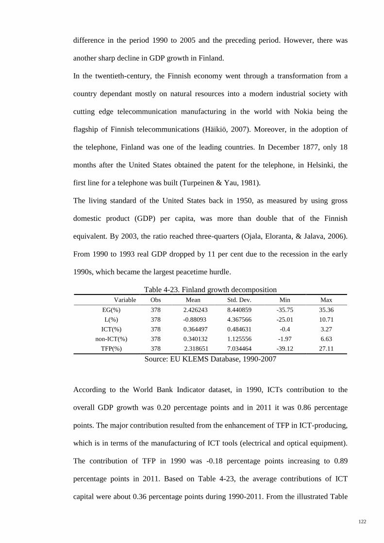
122

difference in the period 1990 to 2005 and the preceding period. However, there was

another sharp decline in GDP growth in Finland.

In the twentieth-century, the Finnish economy went through a transformation from a

country dependant mostly on natural resources into a modern industrial society with

cutting edge telecommunication manufacturing in the world with Nokia being the

flagship of Finnish telecommunications (Häikiö, 2007). Moreover, in the adoption of

the telephone, Finland was one of the leading countries. In December 1877, only 18

months after the United States obtained the patent for the telephone, in Helsinki, the

first line for a telephone was built (Turpeinen & Yau, 1981).

The living standard of the United States back in 1950, as measured by using gross

domestic product (GDP) per capita, was more than double that of the Finnish

equivalent. By 2003, the ratio reached three-quarters (Ojala, Eloranta, & Jalava, 2006).

From 1990 to 1993 real GDP dropped by 11 per cent due to the recession in the early

1990s, which became the largest peacetime hurdle.

Table 4-23. Finland growth decomposition


EG(%) 378 2.426243 8.440859 -35.75 35.36

L(%) 378 -0.88093 4.367566 -25.01 10.71

ICT(%) 378 0.364497 0.484631 -0.4 3.27

non-ICT(%) 378 0.340132 1.125556 -1.97 6.63

TFP(%) 378 2.318651 7.034464 -39.12 27.11


According to the World Bank Indicator dataset, in 1990, ICTs contribution to the

overall GDP growth was 0.20 percentage points and in 2011 it was 0.86 percentage

points. The major contribution resulted from the enhancement of TFP in ICT-producing,

which is in terms of the manufacturing of ICT tools (electrical and optical equipment).

The contribution of TFP in 1990 was -0.18 percentage points increasing to 0.89

percentage points in 2011. Based on Table 4-23, the average contributions of ICT

capital were about 0.36 percentage points during 1990-2011. From the illustrated Table

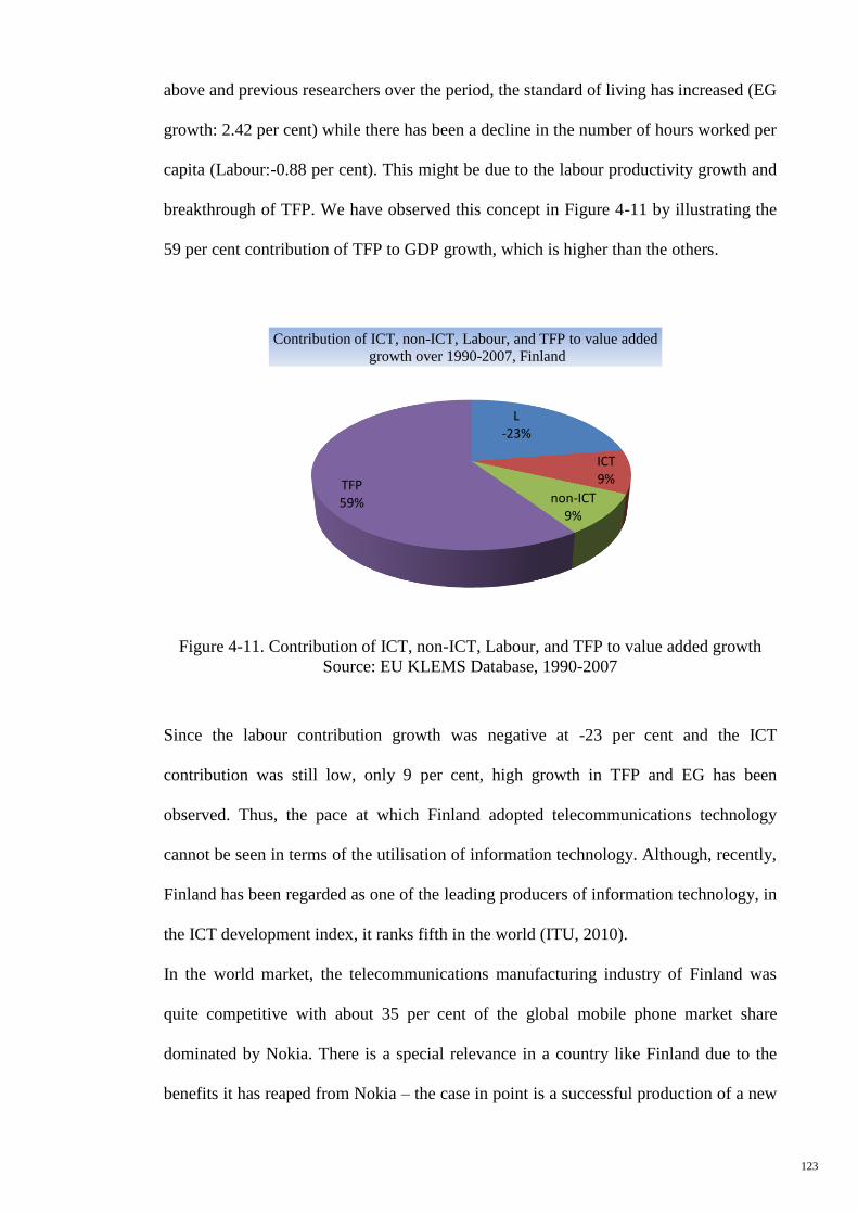
123

above and previous researchers over the period, the standard of living has increased (EG

growth: 2.42 per cent) while there has been a decline in the number of hours worked per

capita (Labour:-0.88 per cent). This might be due to the labour productivity growth and

breakthrough of TFP. We have observed this concept in Figure 4-11 by illustrating the

59 per cent contribution of TFP to GDP growth, which is higher than the others.

Figure 4-11. Contribution of ICT, non-ICT, Labour, and TFP to value added growth


Since the labour contribution growth was negative at -23 per cent and the ICT

contribution was still low, only 9 per cent, high growth in TFP and EG has been

observed. Thus, the pace at which Finland adopted telecommunications technology

cannot be seen in terms of the utilisation of information technology. Although, recently,

Finland has been regarded as one of the leading producers of information technology, in

the ICT development index, it ranks fifth in the world (ITU, 2010).

In the world market, the telecommunications manufacturing industry of Finland was

quite competitive with about 35 per cent of the global mobile phone market share

dominated by Nokia. There is a special relevance in a country like Finland due to the

benefits it has reaped from Nokia – the case in point is a successful production of a new

L -23%

ICT 9%

non-ICT 9%

TFP 59%


growth over 1990-2007, Finland

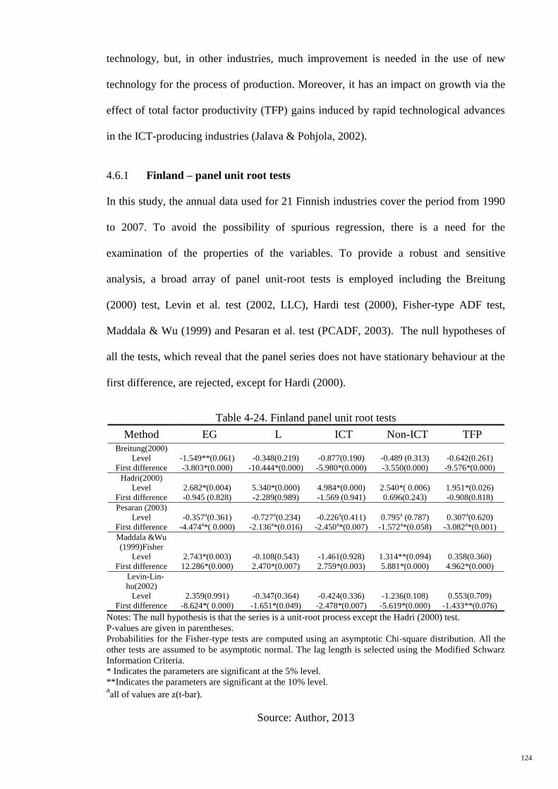
124

technology, but, in other industries, much improvement is needed in the use of new

technology for the process of production. Moreover, it has an impact on growth via the

effect of total factor productivity (TFP) gains induced by rapid technological advances

in the ICT-producing industries (Jalava & Pohjola, 2002).

4.6.1 Finland – panel unit root tests

In this study, the annual data used for 21 Finnish industries cover the period from 1990

to 2007. To avoid the possibility of spurious regression, there is a need for the

examination of the properties of the variables. To provide a robust and sensitive

analysis, a broad array of panel unit-root tests is employed including the Breitung

(2000) test, Levin et al. test (2002, LLC), Hardi test (2000), Fisher-type ADF test,

Maddala & Wu (1999) and Pesaran et al. test (PCADF, 2003). The null hypotheses of

all the tests, which reveal that the panel series does not have stationary behaviour at the

first difference, are rejected, except for Hardi (2000).

Table 4-24. Finland panel unit root tests

Method EG L ICT Non-ICT TFP

Breitung(2000)

Level

First difference

-1.549**(0.061)

-3.803*(0.000)

-0.348(0.219)

-10.444*(0.000)

-0.877(0.190)

-5.980*(0.000)

-0.489 (0.313)

-3.550(0.000)

-0.642(0.261)

-9.576*(0.000)

Hadri(2000)

Level

First difference

2.682*(0.004)

-0.945 (0.828)

5.340*(0.000)

-2.289(0.989)

4.984*(0.000)

-1.569 (0.941)

2.540*( 0.006)

0.696(0.243)

1.951*(0.026)

-0.908(0.818)

Pesaran (2003)

Level

First difference

-0.357a(0.361)

-4.474a*( 0.000)

-0.727a(0.234)

-2.136a*(0.016)

-0.226a(0.411)

-2.450a*(0.007)

0.795a (0.787)

-1.572a*(0.058)

0.307a(0.620)

-3.082a*(0.001)

Maddala &Wu

(1999)Fisher

Level

First difference

2.743*(0.003)

12.286*(0.000)

-0.108(0.543)

2.470*(0.007)

-1.461(0.928)

2.759*(0.003)

1.314**(0.094)

5.881*(0.000)

0.358(0.360)

4.962*(0.000)

Levin-Lin-

hu(2002)

Level

First difference

2.359(0.991)

-8.624*( 0.000)

-0.347(0.364)

-1.651*(0.049)

-0.424(0.336)

-2.478*(0.007)

-1.236(0.108)

-5.619*(0.000)

0.553(0.709)

-1.433**(0.076)

Notes: The null hypothesis is that the series is a unit-root process except the Hadri (2000) test.








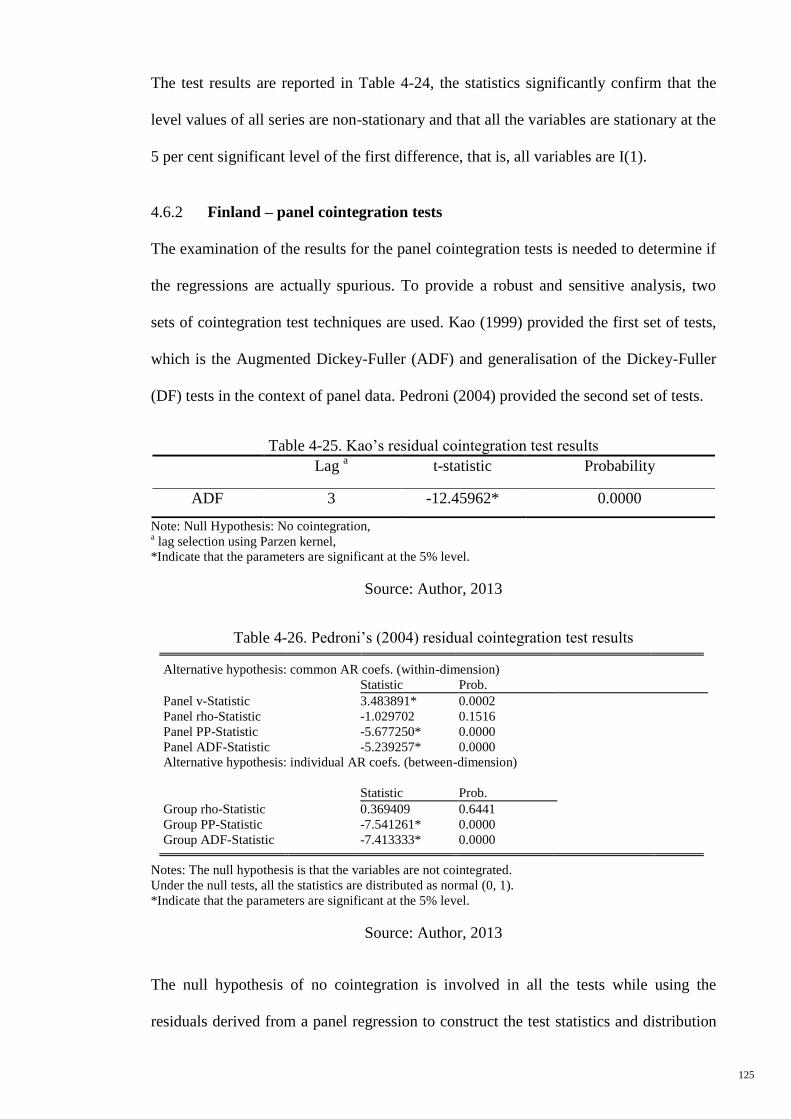
125

The test results are reported in Table 4-24, the statistics significantly confirm that the

level values of all series are non-stationary and that all the variables are stationary at the

5 per cent significant level of the first difference, that is, all variables are I(1).

4.6.2 Finland – panel cointegration tests

The examination of the results for the panel cointegration tests is needed to determine if

the regressions are actually spurious. To provide a robust and sensitive analysis, two

sets of cointegration test techniques are used. Kao (1999) provided the first set of tests,

which is the Augmented Dickey-Fuller (ADF) and generalisation of the Dickey-Fuller

(DF) tests in the context of panel data. Pedroni (2004) provided the second set of tests.



ADF 3 -12.45962* 0.0000





Table 4-26. Pedroni’s (2004) residual cointegration test results Alternative hypothesis: common AR coefs. (within-dimension)

Statistic Prob.


Panel rho-Statistic -1.029702 0.1516




Statistic Prob.








The null hypothesis of no cointegration is involved in all the tests while using the

residuals derived from a panel regression to construct the test statistics and distribution

126

determinants. Asymptotic distribution is found in all the test statistics after appropriate

standardisation. Table 4-26 presents the results of the panel cointegration tests proposed

by Pedroni (1999, 2004). His tests can be classified into two categories. The first set is

similar to the tests illustrated above and involves averaging the test statistics for

cointegration in time series across sections. For the second set, averaging is done in

pieces so that the limiting distributions are based on the limits of piecewise numerator

and denominator terms. As shown in Table 4-26, the Pedroni (2004) heterogeneous

panel statistics reject the null hypothesis of no cointegration when they have large

positive or negative values with the exception for the panel rho-statistic and group rho-

statistic tests, which, at the 5 per cent significance level, do not reject the null

hypothesis of cointegration when it has a small positive or negative value. It is indicated

in the results that the majority of the particular tests reject the null hypothesis of no

cointegration for the Finnish variables. Thus, the estimation of a long run relationship

between the explanatory and dependent variables is possible. The residual panel

cointegration tests of Kao (1999) are reported in Table 4-25, where the null hypothesis

of no cointegration is also rejected at the 5 per cent significant level.

4.6.3 Finland – panel Granger causality results

As seen in Table 4-27, we are not able to see signs of short run causality moving from

ICT and non-ICT to value added growth and TFP, which suggests that GDP and TFP

growth will not be influenced by the contribution of ICT and non-ICT growth. In

addition, it does not possess an effect on these variables in the short run and that the

policies for increasing ICT-producing industries may not retard GDP growth.

In this sense, there is unidirectional causality among ICT, non-ICT and value added

growth as well as among ICT, non-ICT and TFP growth in the short run. Moreover, the

results demonstrate evidence of short run causality between L and EG ,the same as TFP

and EG in the short run, implying that a 1 per cent increase in labour employment and

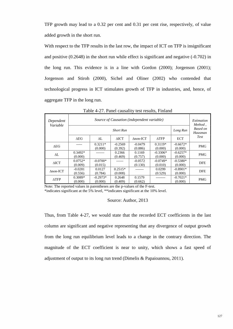
127

TFP growth may lead to a 0.32 per cent and 0.31 per cent rise, respectively, of value

added growth in the short run.

With respect to the TFP results in the last row, the impact of ICT on TFP is insignificant

and positive (0.2648) in the short run while effect is significant and negative (-0.702) in

the long run. This evidence is in a line with Gordon (2000); Jorgenson (2001);

Jorgenson and Stiroh (2000), Sichel and Oliner (2002) who contended that

technological progress in ICT stimulates growth of TFP in industries, and, hence, of

aggregate TFP in the long run.

Table 4-27. Panel causality test results, Finland

Dependent

Variable

Source of Causation (independent variable)

Estimation

Method ,

Based on

Hausman

Test

Short Run Long Run


∆EG ----- 0.3211*

(0.000)

-0.2569

(0.392)

-0.0479

(0.886)

0.3119*

(0.000)

-0.6672*

(0.000) PMG

∆L 0.3492*

(0.000)

-------

0.2366

(0.469)

0.1169

(0.757)

-0.3306*

(0.000)

-0.6257*

(0.000) PMG

∆ICT 0.0752*

(0.009)

-0.0700*

(0.015)

------ -0.0572

(0.130)

-0.0749*

(0.010)

-0.5380*

(0.000) DFE

∆non-ICT -0.0281

(0.556)

0.0127

(0.784)

0.2515*

(0.008)

------- 0.0299

(0.529)

-0.8901*

(0.000) DFE

∆TFP 0.3089*

(0.000)

-0.2973*

(0.000)

0.2648

(0.409)

0.1579

(0.662)

-------- -0.7021*

(0.000) PMG




Thus, from Table 4-27, we would state that the recorded ECT coefficients in the last

column are significant and negative representing that any divergence of output growth

from the long run equilibrium level leads to a change in the contrary direction. The

magnitude of the ECT coefficient is near to unity, which shows a fast speed of

adjustment of output to its long run trend (Dimelis & Papaioannou, 2011).

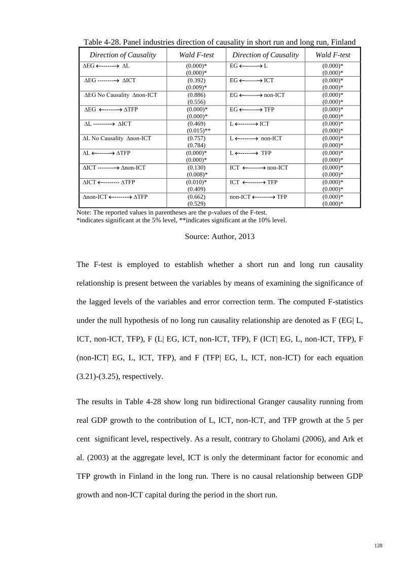
128

Table 4-28. Panel industries direction of causality in short run and long run, Finland




The F-test is employed to establish whether a short run and long run causality

relationship is present between the variables by means of examining the significance of

the lagged levels of the variables and error correction term. The computed F-statistics

under the null hypothesis of no long run causality relationship are denoted as F (EG| L,

ICT, non-ICT, TFP), F (L| EG, ICT, non-ICT, TFP), F (ICT| EG, L, non-ICT, TFP), F

(non-ICT| EG, L, ICT, TFP), and F (TFP| EG, L, ICT, non-ICT) for each equation

(3.21)-(3.25), respectively.

The results in Table 4-28 show long run bidirectional Granger causality running from

real GDP growth to the contribution of L, ICT, non-ICT, and TFP growth at the 5 per

cent significant level, respectively. As a result, contrary to Gholami (2006), and Ark et

al. (2003) at the aggregate level, ICT is only the determinant factor for economic and

TFP growth in Finland in the long run. There is no causal relationship between GDP

growth and non-ICT capital during the period in the short run.


∆EG ------ ∆L

(0.000)*

(0.000)*

EG ------ L

(0.000)*

(0.000)*

∆EG -------- ∆ICT

(0.392)

(0.009)*

EG ------ ICT

(0.000)*

(0.000)*

∆EG No Causality ∆non-ICT

(0.886)

(0.556) EG ------ non-ICT (0.000)*

(0.000)*

∆EG ------ ∆TFP (0.000)*

(0.000)*

EG ------ TFP (0.000)*

(0.000)*

∆L -------- ∆ICT

(0.469)

(0.015)** L ------ ICT

(0.000)*

(0.000)*

∆L No Causality ∆non-ICT

(0.757)

(0.784)

L ------ non-ICT

(0.000)*

(0.000)*

∆L ------ ∆TFP (0.000)*

(0.000)*

L ------ TFP

(0.000)*

(0.000)*

∆ICT -------- ∆non-ICT

(0.130)

(0.008)* ICT ------ non-ICT (0.000)*

(0.000)*

∆ICT -------- ∆TFP (0.010)*

(0.409)

ICT ------ TFP

(0.000)*

(0.000)*

∆non-ICT ------ ∆TFP

(0.662)

(0.529) non-ICT ------ TFP

(0.000)*

(0.000)*

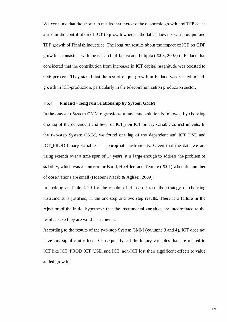
129

We conclude that the short run results that increase the economic growth and TFP cause

a rise in the contribution of ICT to growth whereas the latter does not cause output and

TFP growth of Finnish industries. The long run results about the impact of ICT on GDP

growth is consistent with the research of Jalava and Pohjola (2003, 2007) in Finland that

considered that the contribution from increases in ICT capital magnitude was boosted to

0.46 per cent. They stated that the rest of output growth in Finland was related to TFP

growth in ICT-production, particularly in the telecommunication production sector.

4.6.4 Finland – long run relationship by System GMM

In the one-step System GMM regressions, a moderate solution is followed by choosing

one lag of the dependent and level of ICT_non-ICT binary variable as instruments. In

the two-step System GMM, we found one lag of the dependent and ICT_USE and

ICT_PROD binary variables as appropriate instruments. Given that the data we are

using extends over a time span of 17 years, it is large enough to address the problem of

stability, which was a concern for Bond, Hoeffler, and Temple (2001) when the number

of observations are small (Hosseini Nasab & Aghaei, 2009).

In looking at Table 4-29 for the results of Hansen J test, the strategy of choosing

instruments is justified, in the one-step and two-step results. There is a failure in the

rejection of the initial hypothesis that the instrumental variables are uncorrelated to the

residuals, so they are valid instruments.

According to the results of the two-step System GMM (columns 3 and 4), ICT does not

have any significant effects. Consequently, all the binary variables that are related to

ICT like ICT_PROD ICT_USE, and ICT_non-ICT lost their significant effects to value

added growth.

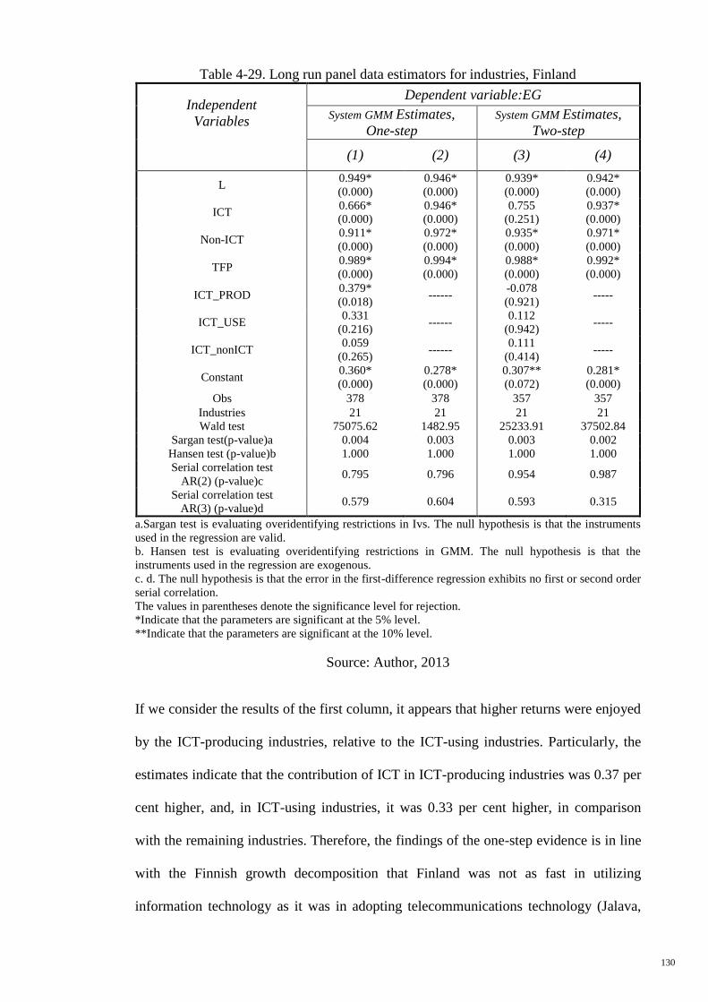
130

Table 4-29. Long run panel data estimators for industries, Finland

Independent

Variables



One-step


Two-step

(1) (2) (3) (4)

L 0.949*

(0.000)

0.946*

(0.000)

0.939*

(0.000)

0.942*

(0.000)

ICT 0.666*

(0.000)

0.946*

(0.000)

0.755

(0.251)

0.937*

(0.000)

Non-ICT 0.911*

(0.000)

0.972*

(0.000)

0.935*

(0.000)

0.971*

(0.000)

TFP 0.989*

(0.000)

0.994*

(0.000)

0.988*

(0.000)

0.992*

(0.000)

ICT_PROD 0.379*

(0.018) ------

-0.078

(0.921) -----

ICT_USE 0.331

(0.216) ------

0.112

(0.942) -----

ICT_nonICT 0.059

(0.265) ------

0.111

(0.414) -----

Constant 0.360*

(0.000)

0.278*

(0.000)

0.307**

(0.072)

0.281*

(0.000)

Obs 378 378 357 357


Wald test 75075.62 1482.95 25233.91 37502.84




AR(2) (p-value)c 0.795 0.796 0.954 0.987


AR(3) (p-value)d 0.579 0.604 0.593 0.315

a.Sargan test is evaluating overidentifying restrictions in Ivs. The null hypothesis is that the instruments




c. d. The null hypothesis is that the error in the first-difference regression exhibits no first or second order

serial correlation.





If we consider the results of the first column, it appears that higher returns were enjoyed

by the ICT-producing industries, relative to the ICT-using industries. Particularly, the

estimates indicate that the contribution of ICT in ICT-producing industries was 0.37 per

cent higher, and, in ICT-using industries, it was 0.33 per cent higher, in comparison

with the remaining industries. Therefore, the findings of the one-step evidence is in line

with the Finnish growth decomposition that Finland was not as fast in utilizing

information technology as it was in adopting telecommunications technology (Jalava,

131

2003; Jalava & Pohjola, 2002, 2007). There is special relevance in a country like

Finland due to the benefits it reaped from Nokia. The case in point is a successful

production of a new technology, while, in other industries, much improvement is

needed to use new technology for the process of production.

Furthermore, ICT has an impact on growth via its strong effect on total factor

productivity (0.98%) gains induced by rapid technological advances in the ICT-

producing industries. However, considering the arguments of O’Mahony (2005) and

Ark et al. (2003), there is a strong potential for the exploitation of growth benefits in the

service industries in Finland where ICT use is intensive. Insignificant coefficient of

ICT_nonICT in columns 1 and 3 show that between ICT and non-ICT capital no

significant complementary effects exist. To sum up, due to the System GMM results,

the largest part of growth in the Finnish sectors is sourced from TFP, non-ICT and ICT,

especially ICT-producing sectors.

On the other hand, the reported results in these columns indicate that the productivity

effects of ICT are significantly higher in the ICT-using industries. It might be concluded

that the beneficial effects of ICTs are not concentrated on investment in ICT-producing

industries in Finland because of the negative effects of ICT-producing industries. In

contrast, the efforts to increase the use of ICT services in companies and industries will

stimulate GDP growth.

4.6.5 Justification of insignificant effects of ICT on TFP and GDP growth in

Finland

Even though it is well known that ICT is a driving force of economic growth there are

still few proofs that show that ICT can also have a negative effect on economic growth.

Furthermore, in the study of 43 countries spanning from 1985 to 1999, no significant

relationship was found between economic growth and ICT investment (Pohjola, 2002).

Another research conducted on 84 countries from the period spanning from 1990 to

132

1999 revealed that there was no significant positive impact on economic growth by the

penetration of computers; however, Jacobsen (2003) did find a positive relationship

between economic growth and mobile phones (Jacobsen, 2003). The negative

contribution to economic growth by computers due to the high cost of new ICT

investment is explained by the application of the traditional growth accounting

framework in the US (Kiley, 1999).

Computers and related services are sectors that account for much of the production of

software. In Finland, in the last 30 years, the share of business sector value added has

been increased by service-related ICT-industries (Eberhardt, 2011). Previous research

indicated that, in Finland, a significant role has been played by the ICT sector since the

mid-1990s. Therefore, it is concluded that Finland depends more on ICT-production to

further boost economic growth.

Hence, based on the GDP share of the ICT-producing sector (5.41 per cent), which is

“electrical and optical equipment” industries, it is claimed that the “Nokia” company,

which is one of the well-known producers of mobile phones in the last decade, has

performed poorly in marketing and updating smart phone applications for contributing

more GDP growth. Although in Finland there was a five-fold rise in the contribution of

“electrical and optical equipment” from 4.78 per cent to 20.7 per cent between 1990 and

2007, recently, Finland’s telecommunications manufacturing industry (Nokia) has lost

competitive power in the world market, which is probably the essential driver of

economic growth. Remarkably, however, the diffusion of ICT has become sluggish in

Finland compared to some other EU countries calculated by the portion of software

packages in private non-residential fixed properties (Jalava & Pohjola, 2008).

Justification for the use of the “electrical and optical equipment" industry can be derived

from the studies of Jorgenson and Stiroh (2003) who found that much of the recent US

growth recovery occurred in ICT producing sectors. Thus, in this research “electrical

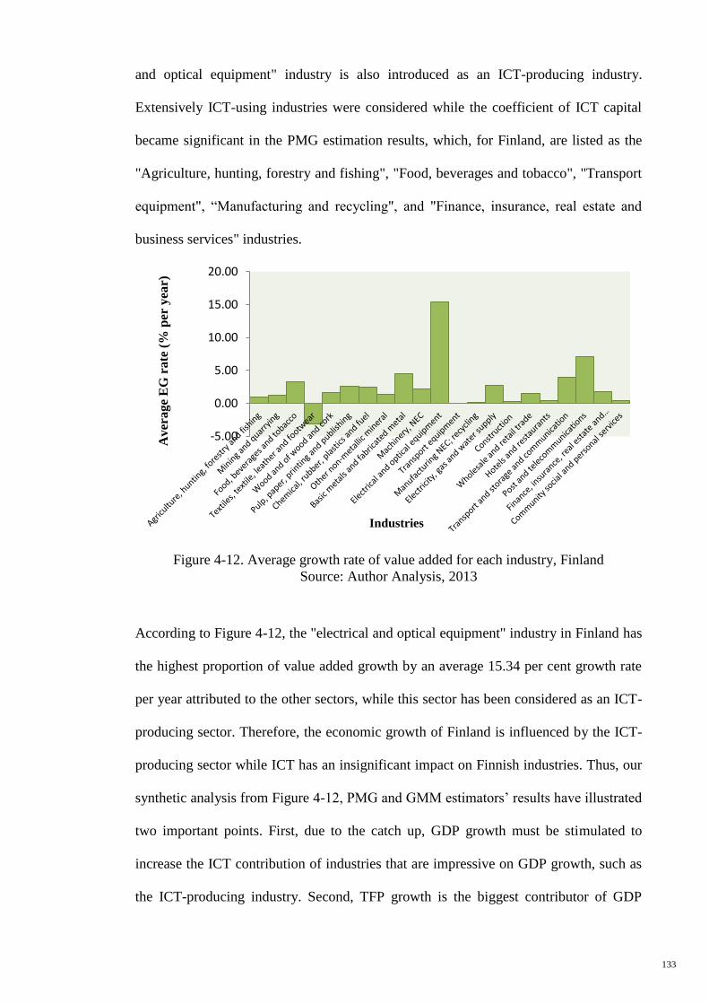
http://www.plosone.org/article/info%3Adoi%2F10.1371%2Fjournal.pone.0048903#pone.0048903-Jacobsen1

133

and optical equipment" industry is also introduced as an ICT-producing industry.

Extensively ICT-using industries were considered while the coefficient of ICT capital

became significant in the PMG estimation results, which, for Finland, are listed as the

"Agriculture, hunting, forestry and fishing", "Food, beverages and tobacco", "Transport

equipment", “Manufacturing and recycling", and "Finance, insurance, real estate and

business services" industries.

Figure 4-12. Average growth rate of value added for each industry, Finland


According to Figure 4-12, the "electrical and optical equipment" industry in Finland has

the highest proportion of value added growth by an average 15.34 per cent growth rate

per year attributed to the other sectors, while this sector has been considered as an ICT-

producing sector. Therefore, the economic growth of Finland is influenced by the ICT-

producing sector while ICT has an insignificant impact on Finnish industries. Thus, our

synthetic analysis from Figure 4-12, PMG and GMM estimators’ results have illustrated

two important points. First, due to the catch up, GDP growth must be stimulated to

increase the ICT contribution of industries that are impressive on GDP growth, such as

the ICT-producing industry. Second, TFP growth is the biggest contributor of GDP

-5.00

0.00

5.00

10.00

15.00

20.00

Aver

age

EG

ra

te (

% p

er y

ear)

Industries

134

growth in Finland (59 per cent). Based on the causality results, ICT is not a source of

TFP growth in the short run, thus GDP growth in the long run could not attribute to the

spillover effects of ICT through TFP growth. The finding is fascinating because we are

unaware of the solid evidence for ICT spillovers within Finland. The proof is weak, as it

seems to be for the period 1990-2011; therefore ICT is not effective on GDP growth,

which leads to the insignificant effects of ICT on value added growth.

The difference in the impacts of TFP and ICT investments from ICT goods production

can partially explain the Intra-EU differences of labour productivity growth. There was

a strong decline in the productivity growth rates in some of the EU’s largest economies

like Italy, France, the UK, Germany, and, more importantly, Spain. While, smaller

countries were facing acceleration in their labour productivity growth, such as Austria,

Finland, Sweden and Ireland, it is not easy to explain these differences. The increased

availability of ICT might be a factor as well as to how there are different responses to

the provided opportunities, such as different industrial structures and varying degrees of

openness of the economies.

It has been shown in various studies that in the US a major role has been played by the

rapid technological development in the ICT-producing industries in the revival of TFP

growth (Jorgenson et al., 2005; Oliner & Sichel, 2002; Jorgenson, 2001). On average,

the GDP share of the ICT producing industries is not similar among European countries,

which may be one of the reasons for the more sluggish TFP growth in Europe over 1995

to 2001. Although the GDP share for ICT-production differs among the European

countries, it may also be a driver of intra-EU differences in TFP growth. Within the EU,

it has been argued that productivity differentials between the member countries is

related to non-ICT sources (Timmer & Van Ark, 2005), while the benefits from high

shares of ICT-goods production and high ICT capital investment were reaped by some

EU countries, such as Sweden, Finland and Denmark.

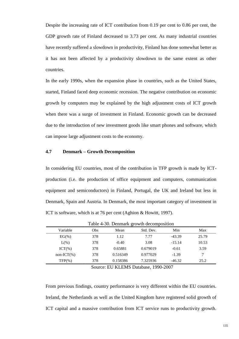
135

Despite the increasing rate of ICT contribution from 0.19 per cent to 0.86 per cent, the

GDP growth rate of Finland decreased to 3.73 per cent. As many industrial countries

have recently suffered a slowdown in productivity, Finland has done somewhat better as

it has not been affected by a productivity slowdown to the same extent as other

countries.

In the early 1990s, when the expansion phase in countries, such as the United States,

started, Finland faced deep economic recession. The negative contribution on economic

growth by computers may be explained by the high adjustment costs of ICT growth

when there was a surge of investment in Finland. Economic growth can be decreased

due to the introduction of new investment goods like smart phones and software, which

can impose large adjustment costs to the economy.

4.7 Denmark – Growth Decomposition

In considering EU countries, most of the contribution in TFP growth is made by ICT-

production (i.e. the production of office equipment and computers, communication

equipment and semiconductors) in Finland, Portugal, the UK and Ireland but less in

Denmark, Spain and Austria. In Denmark, the most important category of investment in

ICT is software, which is at 76 per cent (Aghion & Howitt, 1997).

Table 4-30. Denmark growth decomposition


EG(%) 378 1.12 7.77 -43.39 25.79

L(%) 378 -0.40 3.08 -15.14 10.53

ICT(%) 378 0.65881 0.679019 -0.61 3.59

non-ICT(%) 378 0.516349 0.977029 -1.39 7

TFP(%) 378 0.158386 7.325936 -46.32 25.2


From previous findings, country performance is very different within the EU countries.

Ireland, the Netherlands as well as the United Kingdom have registered solid growth of

ICT capital and a massive contribution from ICT service runs to productivity growth.

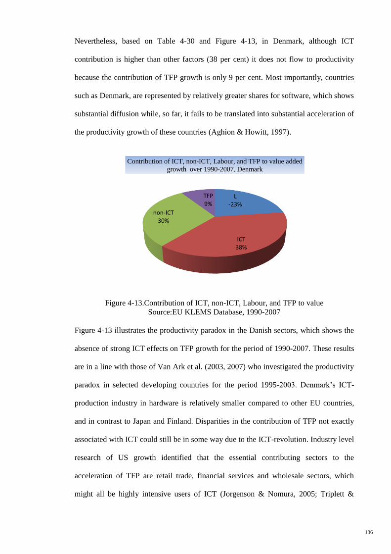
136

Nevertheless, based on Table 4-30 and Figure 4-13, in Denmark, although ICT

contribution is higher than other factors (38 per cent) it does not flow to productivity

because the contribution of TFP growth is only 9 per cent. Most importantly, countries

such as Denmark, are represented by relatively greater shares for software, which shows

substantial diffusion while, so far, it fails to be translated into substantial acceleration of

the productivity growth of these countries (Aghion & Howitt, 1997).

Figure 4-13.Contribution of ICT, non-ICT, Labour, and TFP to value

Source:EU KLEMS Database, 1990-2007

Figure 4-13 illustrates the productivity paradox in the Danish sectors, which shows the

absence of strong ICT effects on TFP growth for the period of 1990-2007. These results

are in a line with those of Van Ark et al. (2003, 2007) who investigated the productivity

paradox in selected developing countries for the period 1995-2003. Denmark’s ICT-

production industry in hardware is relatively smaller compared to other EU countries,

and in contrast to Japan and Finland. Disparities in the contribution of TFP not exactly

associated with ICT could still be in some way due to the ICT-revolution. Industry level

research of US growth identified that the essential contributing sectors to the

acceleration of TFP are retail trade, financial services and wholesale sectors, which

might all be highly intensive users of ICT (Jorgenson & Nomura, 2005; Triplett &

L -23%

ICT 38%

non-ICT 30%

TFP 9%


growth over 1990-2007, Denmark

137

Bosworth, 2004; Triplett, 1999). If one country has higher ICT-using sectors, it will

create positive spillover on TFP growth. On the other hand, countries with higher levels

of ICT investment like Finland as well as Sweden had excessive TFP growth rates.

However, in other ICT intensive countries like Denmark and Japan, TFP growth held

slowed down.

4.7.1 Denmark – panel unit root tests

Before running the cointegration approaches, we have to verify the order of integration

of each variable. Implementing the panel unit root tests, formulated by Maddala & Wu

(1999), Breitung (2000), Hadri (2000), and Levin et al. (2002), which prohibit for

heterogeneity in the autoregressive coefficient, will probably be the solution to identify

the integration order. These tests, as the first generation panel unit root tests, include the

disadvantage of presuming independent cross-sections. On the other hand, it has been

found in the literature that cross-section dependency may arise as a result of several

unobserved reasons, externalities, regional and macroeconomic linkages and also

unaccounted residual interdependence.

Currently, a number of the new panel unit root tests have emerged that resolve the

question of the dependence, and, also, the correlation presented the popularity of

macroeconomic dynamics and linkages. These types of test are named the second-

generation panel unit root tests. A well-known second-generation test is regarded in this

research as Pesaran’s (2003) cross-sectional. We have applied the first and second-

generation panel unit root test.

The findings of the first and second-generation panel unit root tests without trend are

both presented in Table 4-31. For most of the five variables (except ICT in Breitung and

Pesaran tests and TFP in the Levin-Lin-Chu test), the null hypothesis of the unit roots

could not be rejected at level. The outputs robustly reveal that the variables at level are

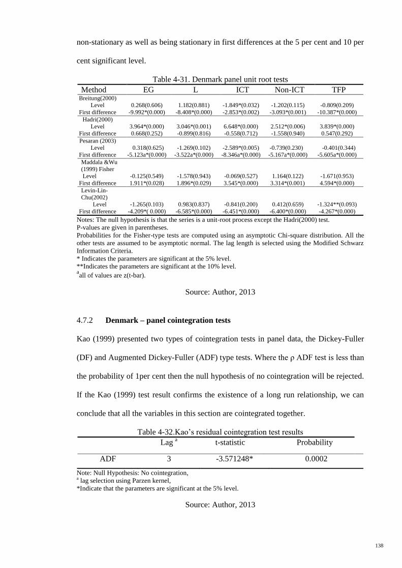
138

non-stationary as well as being stationary in first differences at the 5 per cent and 10 per

cent significant level.

Table 4-31. Denmark panel unit root tests

Method EG L ICT Non-ICT TFP Breitung(2000)

Level

First difference

0.268(0.606)

-9.992*(0.000)

1.182(0.881)

-8.408*(0.000)

-1.849*(0.032)

-2.853*(0.002)

-1.202(0.115)

-3.093*(0.001)

-0.809(0.209)

-10.387*(0.000)

Hadri(2000)

Level

First difference

3.964*(0.000)

0.668(0.252)

3.046*(0.001)

-0.899(0.816)

6.648*(0.000)

-0.558(0.712)

2.512*(0.006)

-1.558(0.940)

3.839*(0.000)

0.547(0.292)

Pesaran (2003)

Level

First difference

0.318(0.625)

-5.123a*(0.000)

-1.269(0.102)

-3.522a*(0.000)

-2.589*(0.005)

-8.346a*(0.000)

-0.739(0.230)

-5.167a*(0.000)

-0.401(0.344)

-5.605a*(0.000)

Maddala &Wu

(1999) Fisher

Level

First difference

-0.125(0.549)

1.911*(0.028)

-1.578(0.943)

1.896*(0.029)

-0.069(0.527)

3.545*(0.000)

1.164(0.122)

3.314*(0.001)

-1.671(0.953)

4.594*(0.000)

Levin-Lin-

Chu(2002)

Level

First difference

-1.265(0.103)

-4.209*( 0.000)

0.983(0.837)

-6.585*(0.000)

-0.841(0.200)

-6.451*(0.000)

0.412(0.659)

-6.400*(0.000)

-1.324**(0.093)

-4.267*(0.000)

Notes: The null hypothesis is that the series is a unit-root process except the Hadri(2000) test.








4.7.2 Denmark – panel cointegration tests

Kao (1999) presented two types of cointegration tests in panel data, the Dickey-Fuller

(DF) and Augmented Dickey-Fuller (ADF) type tests. Where the ρ ADF test is less than

the probability of 1per cent then the null hypothesis of no cointegration will be rejected.

If the Kao (1999) test result confirms the existence of a long run relationship, we can

conclude that all the variables in this section are cointegrated together.

Table 4-32.Kao’s residual cointegration test results


ADF 3 -3.571248* 0.0002

Note: Null Hypothesis: No cointegration, a lag selection using Parzen kernel,



https://www.google.com/url?sa=t&rct=j&q=&esrc=s&source=web&cd=1&ved=0CDIQFjAA&url=http%3A%2F%2Fen.wikipedia.org%2Fwiki%2FAugmented_Dickey%25E2%2580%2593Fuller_test&ei=BVSfUa-0N8H-rAeBnYH4Dg&usg=AFQjCNGAiCaHZoKHP7AEnaK3VRylQ2_BPQ&sig2=trym2UYhoYyJke1KJ0o2Lw

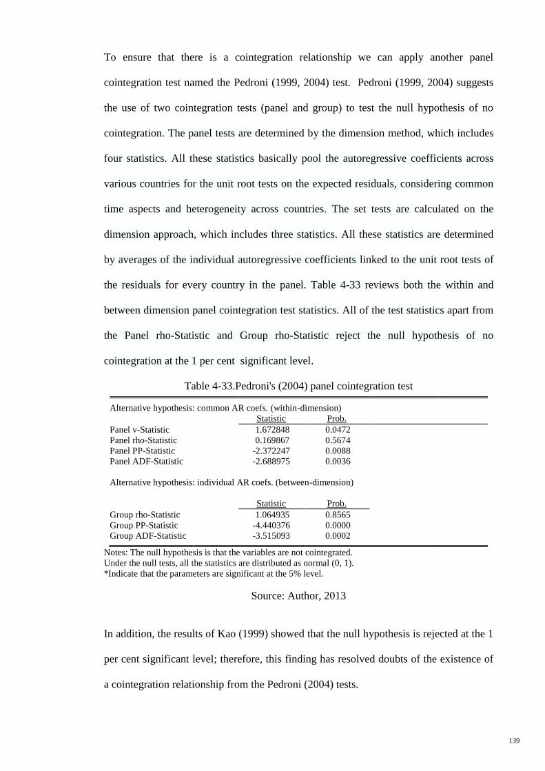
139

To ensure that there is a cointegration relationship we can apply another panel

cointegration test named the Pedroni (1999, 2004) test. Pedroni (1999, 2004) suggests

the use of two cointegration tests (panel and group) to test the null hypothesis of no

cointegration. The panel tests are determined by the dimension method, which includes

four statistics. All these statistics basically pool the autoregressive coefficients across

various countries for the unit root tests on the expected residuals, considering common

time aspects and heterogeneity across countries. The set tests are calculated on the

dimension approach, which includes three statistics. All these statistics are determined

by averages of the individual autoregressive coefficients linked to the unit root tests of

the residuals for every country in the panel. Table 4-33 reviews both the within and

between dimension panel cointegration test statistics. All of the test statistics apart from

the Panel rho-Statistic and Group rho-Statistic reject the null hypothesis of no

cointegration at the 1 per cent significant level.

Table 4-33.Pedroni's (2004) panel cointegration test Alternative hypothesis: common AR coefs. (within-dimension)

Statistic Prob.

Panel v-Statistic 1.672848 0.0472


Panel PP-Statistic -2.372247 0.0088

Panel ADF-Statistic -2.688975 0.0036


Statistic Prob.


Group PP-Statistic -4.440376 0.0000

Group ADF-Statistic -3.515093 0.0002





In addition, the results of Kao (1999) showed that the null hypothesis is rejected at the 1

per cent significant level; therefore, this finding has resolved doubts of the existence of

a cointegration relationship from the Pedroni (2004) tests.

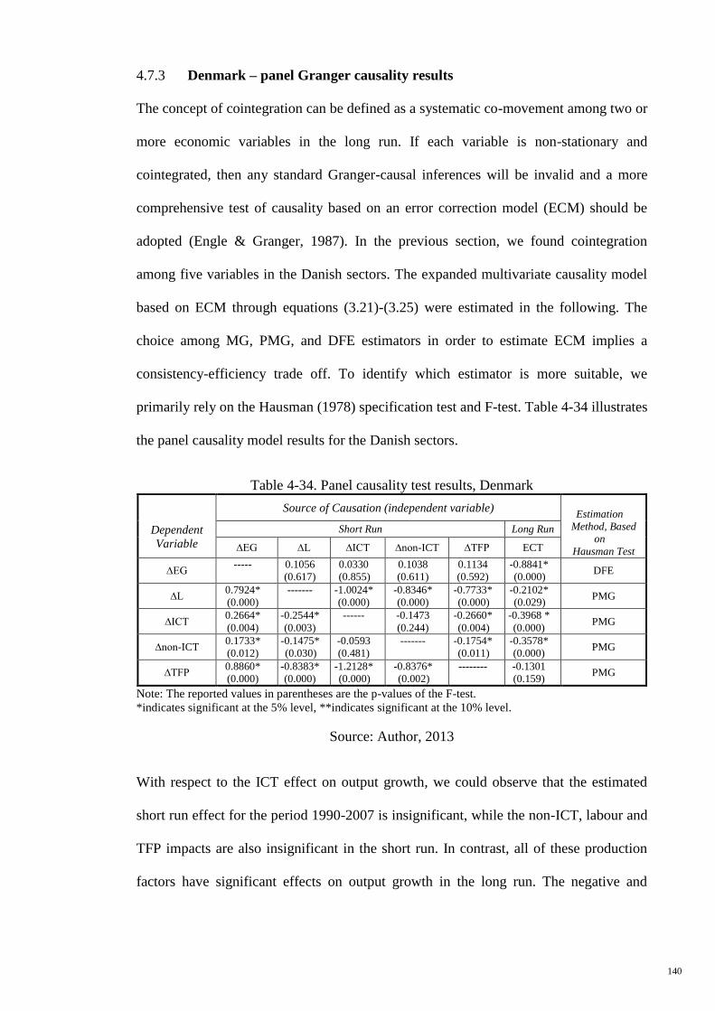
140

4.7.3 Denmark – panel Granger causality results

The concept of cointegration can be defined as a systematic co-movement among two or

more economic variables in the long run. If each variable is non-stationary and

cointegrated, then any standard Granger-causal inferences will be invalid and a more

comprehensive test of causality based on an error correction model (ECM) should be

adopted (Engle & Granger, 1987). In the previous section, we found cointegration

among five variables in the Danish sectors. The expanded multivariate causality model

based on ECM through equations (3.21)-(3.25) were estimated in the following. The

choice among MG, PMG, and DFE estimators in order to estimate ECM implies a

consistency-efficiency trade off. To identify which estimator is more suitable, we

primarily rely on the Hausman (1978) specification test and F-test. Table 4-34 illustrates

the panel causality model results for the Danish sectors.

Table 4-34. Panel causality test results, Denmark

Dependent

Variable


Estimation

Method, Based

on

Hausman Test

Short Run Long Run


∆EG ----- 0.1056

(0.617)

0.0330

(0.855)

0.1038

(0.611)

0.1134

(0.592)

-0.8841*

(0.000) DFE

∆L 0.7924*

(0.000)

-------

-1.0024*

(0.000)

-0.8346*

(0.000)

-0.7733*

(0.000)

-0.2102*

(0.029) PMG

∆ICT 0.2664*

(0.004)

-0.2544*

(0.003)

------ -0.1473

(0.244)

-0.2660*

(0.004)

-0.3968 *

(0.000) PMG

∆non-ICT 0.1733*

(0.012)

-0.1475*

(0.030)

-0.0593

(0.481)

------- -0.1754*

(0.011)

-0.3578*

(0.000) PMG

∆TFP 0.8860*

(0.000)

-0.8383*

(0.000)

-1.2128*

(0.000)

-0.8376*

(0.002)

-------- -0.1301

(0.159) PMG




With respect to the ICT effect on output growth, we could observe that the estimated

short run effect for the period 1990-2007 is insignificant, while the non-ICT, labour and

TFP impacts are also insignificant in the short run. In contrast, all of these production

factors have significant effects on output growth in the long run. The negative and

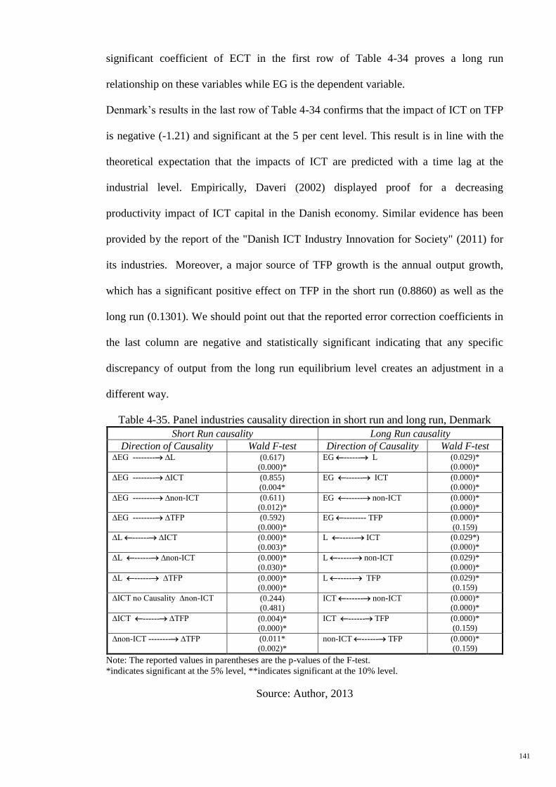
141

significant coefficient of ECT in the first row of Table 4-34 proves a long run

relationship on these variables while EG is the dependent variable.

Denmark’s results in the last row of Table 4-34 confirms that the impact of ICT on TFP

is negative (-1.21) and significant at the 5 per cent level. This result is in line with the

theoretical expectation that the impacts of ICT are predicted with a time lag at the

industrial level. Empirically, Daveri (2002) displayed proof for a decreasing

productivity impact of ICT capital in the Danish economy. Similar evidence has been

provided by the report of the "Danish ICT Industry Innovation for Society" (2011) for

its industries. Moreover, a major source of TFP growth is the annual output growth,

which has a significant positive effect on TFP in the short run (0.8860) as well as the

long run (0.1301). We should point out that the reported error correction coefficients in

the last column are negative and statistically significant indicating that any specific

discrepancy of output from the long run equilibrium level creates an adjustment in a

different way.

Table 4-35. Panel industries causality direction in short run and long run, Denmark




Short Run causality Long Run causality Direction of Causality Wald F-test Direction of Causality Wald F-test

∆EG -------- ∆L

(0.617)

(0.000)*

EG ------ L

(0.029)*

(0.000)*

∆EG -------- ∆ICT

(0.855)

(0.004*

EG ------ ICT

(0.000)*

(0.000)*

∆EG -------- ∆non-ICT (0.611)

(0.012)* EG ------ non-ICT (0.000)*

(0.000)*

∆EG -------- ∆TFP (0.592)

(0.000)*

EG -------- TFP (0.000)*

(0.159)

∆L ------ ∆ICT

(0.000)*

(0.003)*

L ------ ICT

(0.029*)

(0.000)*

∆L ------ ∆non-ICT

(0.000)*

(0.030)*

L ------ non-ICT

(0.029)*

(0.000)*

∆L ------ ∆TFP

(0.000)*

(0.000)*

L ------ TFP

(0.029)*

(0.159)

∆ICT no Causality ∆non-ICT

(0.244)

(0.481)

ICT ------ non-ICT

(0.000)*

(0.000)*

∆ICT ------ ∆TFP (0.004)*

(0.000)*

ICT ------ TFP (0.000)*

(0.159)

∆non-ICT -------- ∆TFP (0.011*

(0.002)*

non-ICT ------ TFP (0.000)*

(0.159)

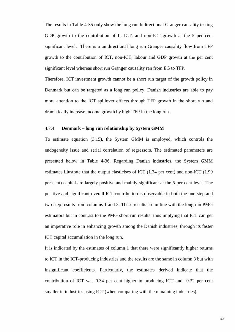
142

The results in Table 4-35 only show the long run bidirectional Granger causality testing

GDP growth to the contribution of L, ICT, and non-ICT growth at the 5 per cent

significant level. There is a unidirectional long run Granger causality flow from TFP

growth to the contribution of ICT, non-ICT, labour and GDP growth at the per cent

significant level whereas short run Granger causality ran from EG to TFP.

Therefore, ICT investment growth cannot be a short run target of the growth policy in

Denmark but can be targeted as a long run policy. Danish industries are able to pay

more attention to the ICT spillover effects through TFP growth in the short run and

dramatically increase income growth by high TFP in the long run.

4.7.4 Denmark – long run relationship by System GMM

To estimate equation (3.15), the System GMM is employed, which controls the

endogeneity issue and serial correlation of regressors. The estimated parameters are

presented below in Table 4-36. Regarding Danish industries, the System GMM

estimates illustrate that the output elasticises of ICT (1.34 per cent) and non-ICT (1.99

per cent) capital are largely positive and mainly significant at the 5 per cent level. The

positive and significant overall ICT contribution is observable in both the one-step and

two-step results from columns 1 and 3. These results are in line with the long run PMG

estimators but in contrast to the PMG short run results; thus implying that ICT can get

an imperative role in enhancing growth among the Danish industries, through its faster

ICT capital accumulation in the long run.

It is indicated by the estimates of column 1 that there were significantly higher returns

to ICT in the ICT-producing industries and the results are the same in column 3 but with

insignificant coefficients. Particularly, the estimates derived indicate that the

contribution of ICT was 0.34 per cent higher in producing ICT and -0.32 per cent

smaller in industries using ICT (when comparing with the remaining industries).

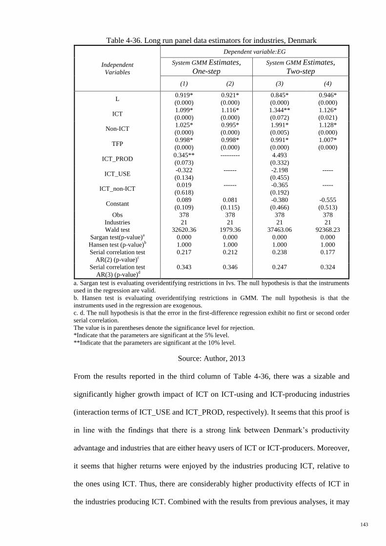
143

Table 4-36. Long run panel data estimators for industries, Denmark

Independent

Variables



One-step


Two-step

(1) (2) (3) (4)

L 0.919*

(0.000)

0.921*

(0.000)

0.845*

(0.000)

0.946*

(0.000)

ICT 1.099*

(0.000)

1.116*

(0.000)

1.344**

(0.072)

1.126*

(0.021)

Non-ICT 1.025*

(0.000)

0.995*

(0.000)

1.991*

(0.005)

1.128*

(0.000)

TFP 0.998*

(0.000)

0.998*

(0.000)

0.991*

(0.000)

1.007*

(0.000)

ICT_PROD 0.345**

(0.073)

--------- 4.493

(0.332)

ICT_USE -0.322

(0.134)

------ -2.198

(0.455)

-----

ICT_non-ICT 0.019

(0.618)

------ -0.365

(0.192)

-----

Constant 0.089

(0.109)

0.081

(0.115)

-0.380

(0.466)

-0.555

(0.513)

Obs 378 378 378 378


Wald test 32620.36 1979.36 37463.06 92368.23




AR(2) (p-value)c

0.217 0.212 0.238 0.177


AR(3) (p-value)d

0.343 0.346 0.247 0.324






serial correlation.

The value is in parentheses denote the significance level for rejection.




From the results reported in the third column of Table 4-36, there was a sizable and

significantly higher growth impact of ICT on ICT-using and ICT-producing industries

(interaction terms of ICT_USE and ICT_PROD, respectively). It seems that this proof is

in line with the findings that there is a strong link between Denmark’s productivity

advantage and industries that are either heavy users of ICT or ICT-producers. Moreover,

it seems that higher returns were enjoyed by the industries producing ICT, relative to

the ones using ICT. Thus, there are considerably higher productivity effects of ICT in

the industries producing ICT. Combined with the results from previous analyses, it may

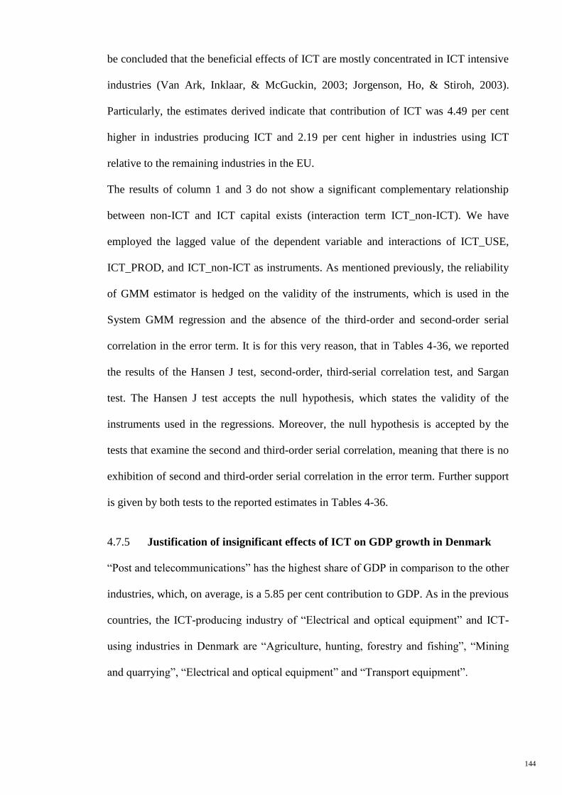
144

be concluded that the beneficial effects of ICT are mostly concentrated in ICT intensive

industries (Van Ark, Inklaar, & McGuckin, 2003; Jorgenson, Ho, & Stiroh, 2003).

Particularly, the estimates derived indicate that contribution of ICT was 4.49 per cent

higher in industries producing ICT and 2.19 per cent higher in industries using ICT

relative to the remaining industries in the EU.

The results of column 1 and 3 do not show a significant complementary relationship

between non-ICT and ICT capital exists (interaction term ICT_non-ICT). We have

employed the lagged value of the dependent variable and interactions of ICT_USE,

ICT_PROD, and ICT_non-ICT as instruments. As mentioned previously, the reliability

of GMM estimator is hedged on the validity of the instruments, which is used in the

System GMM regression and the absence of the third-order and second-order serial

correlation in the error term. It is for this very reason, that in Tables 4-36, we reported

the results of the Hansen J test, second-order, third-serial correlation test, and Sargan

test. The Hansen J test accepts the null hypothesis, which states the validity of the

instruments used in the regressions. Moreover, the null hypothesis is accepted by the

tests that examine the second and third-order serial correlation, meaning that there is no

exhibition of second and third-order serial correlation in the error term. Further support

is given by both tests to the reported estimates in Tables 4-36.

4.7.5 Justification of insignificant effects of ICT on GDP growth in Denmark

“Post and telecommunications” has the highest share of GDP in comparison to the other

industries, which, on average, is a 5.85 per cent contribution to GDP. As in the previous

countries, the ICT-producing industry of “Electrical and optical equipment” and ICT-

using industries in Denmark are “Agriculture, hunting, forestry and fishing”, “Mining

and quarrying”, “Electrical and optical equipment” and “Transport equipment”.

145

Figure 4-14. Average growth rate of value added for each industry, Denmark

Source: Author’s computation based on dataset from EUKLEMS, 2013

ICT-producing industry has positive significant effects on GDP growth via a 5.14 per

cent average contribution to GDP, whereas ICT-using industries have negative

insignificant effects on GDP growth via an average 2.46 per cent contribution to GDP.

Therefore, despite the positive effects of ICT-producing industry on GDP, more

investment in the growth of “Post and telecommunications” is capable of being an

engine of GDP growth for Danish industries.

With reference to the previous sections, ICT with more than a 38 per cent contribution

to GDP growth is introduced as the main contributor of output growth, while non-ICT is

ranked second with a 30 per cent contribution. Therefore, despite the significant effects

of ICT on TFP, the insignificant direct effects of ICT have dominated the spillover

effects of ICT. Thus, overall, there are no significant effects of ICT contribution for the

Danish sectors.

The limited number of ICT-using industries (only 4 industries) is one of the problems of

Danish industries limited diffusion and penetration of ICT. These industries also have

insignificant and negative effects on GDP growth. The spillover effects of ICT would

-6.00

-4.00

-2.00

0.00

2.00

4.00

6.00

8.00

Ave

rage

EG

rat

e (

% p

er

year

)

Industries

146

emerge in all dimensions when the use of ICT becomes widespread in the majority of

industries, especially in the key industries of each country. Promoting ICT diffusion

among sectors guarantees huge profits for firm competitiveness and economic growth.

This is possibly because several EU countries are generally so powerful in developing

their ICT-producing industries, ICT diffusion by means of computerization and Internet

application is the key to the growth and competitiveness of their economies.

Moreover, Denmark’s ICT hardware industry has not become a major driver of

economic growth because of the lack of its government’s strategic support of the

industry's formation and development.

In summing up, it is vital for the Danish government to consider the opportunity of

increasing ICT-use in different industries (Vu, 2009). The long run significant effects of

ICT show that Denmark is a significantly developed ICT country as well as being a

solid environment for strengthening and addressing social and consumer driven

requirements, such as health and climate linked concerns. The Danish digital eco-

system has a strong technological foundation for system development, integrating

hardware and software embedded systems. It also comprises one of the most

competitive and advanced telecommunications infrastructure and mobile markets. This

will be central for the development of new smart products for applications in health,

energy and environment and the future Internet ("Danish ICT Industry Innovation for

Society," 2011).

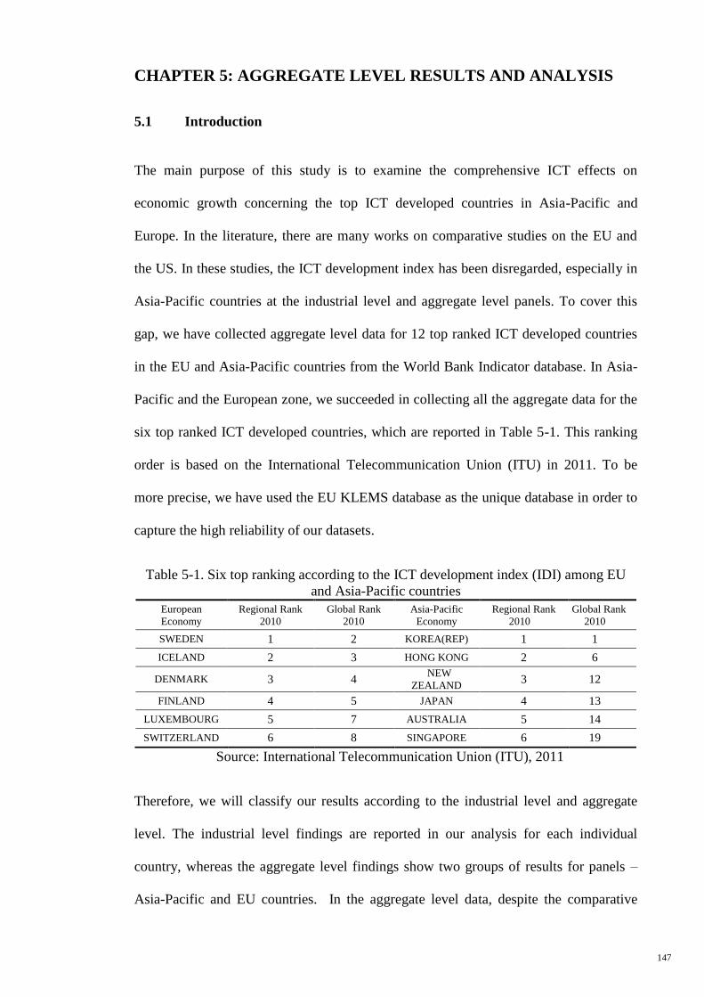
147

5 CHAPTER 5: AGGREGATE LEVEL RESULTS AND ANALYSIS

5.1 Introduction

The main purpose of this study is to examine the comprehensive ICT effects on

economic growth concerning the top ICT developed countries in Asia-Pacific and

Europe. In the literature, there are many works on comparative studies on the EU and

the US. In these studies, the ICT development index has been disregarded, especially in

Asia-Pacific countries at the industrial level and aggregate level panels. To cover this

gap, we have collected aggregate level data for 12 top ranked ICT developed countries

in the EU and Asia-Pacific countries from the World Bank Indicator database. In Asia-

Pacific and the European zone, we succeeded in collecting all the aggregate data for the

six top ranked ICT developed countries, which are reported in Table 5-1. This ranking

order is based on the International Telecommunication Union (ITU) in 2011. To be

more precise, we have used the EU KLEMS database as the unique database in order to

capture the high reliability of our datasets.

Table 5-1. Six top ranking according to the ICT development index (IDI) among EU

and Asia-Pacific countries

European

Economy

Regional Rank

2010

Global Rank

2010

Asia-Pacific

Economy

Regional Rank

2010

Global Rank

2010



DENMARK 3 4 NEW

ZEALAND 3 12





Therefore, we will classify our results according to the industrial level and aggregate

level. The industrial level findings are reported in our analysis for each individual

country, whereas the aggregate level findings show two groups of results for panels –

Asia-Pacific and EU countries. In the aggregate level data, despite the comparative

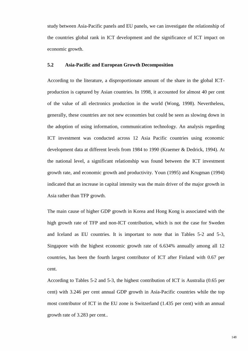
148

study between Asia-Pacific panels and EU panels, we can investigate the relationship of

the countries global rank in ICT development and the significance of ICT impact on

economic growth.

5.2 Asia-Pacific and European Growth Decomposition

According to the literature, a disproportionate amount of the share in the global ICT-

production is captured by Asian countries. In 1998, it accounted for almost 40 per cent

of the value of all electronics production in the world (Wong, 1998). Nevertheless,

generally, these countries are not new economies but could be seen as slowing down in

the adoption of using information, communication technology. An analysis regarding

ICT investment was conducted across 12 Asia Pacific countries using economic

development data at different levels from 1984 to 1990 (Kraemer & Dedrick, 1994). At

the national level, a significant relationship was found between the ICT investment

growth rate, and economic growth and productivity. Youn (1995) and Krugman (1994)

indicated that an increase in capital intensity was the main driver of the major growth in

Asia rather than TFP growth.

The main cause of higher GDP growth in Korea and Hong Kong is associated with the

high growth rate of TFP and non-ICT contribution, which is not the case for Sweden

and Iceland as EU countries. It is important to note that in Tables 5-2 and 5-3,

Singapore with the highest economic growth rate of 6.634% annually among all 12

countries, has been the fourth largest contributor of ICT after Finland with 0.67 per

cent.

According to Tables 5-2 and 5-3, the highest contribution of ICT is Australia (0.65 per

cent) with 3.246 per cent annual GDP growth in Asia-Pacific countries while the top

most contributor of ICT in the EU zone is Switzerland (1.435 per cent) with an annual

growth rate of 3.283 per cent..

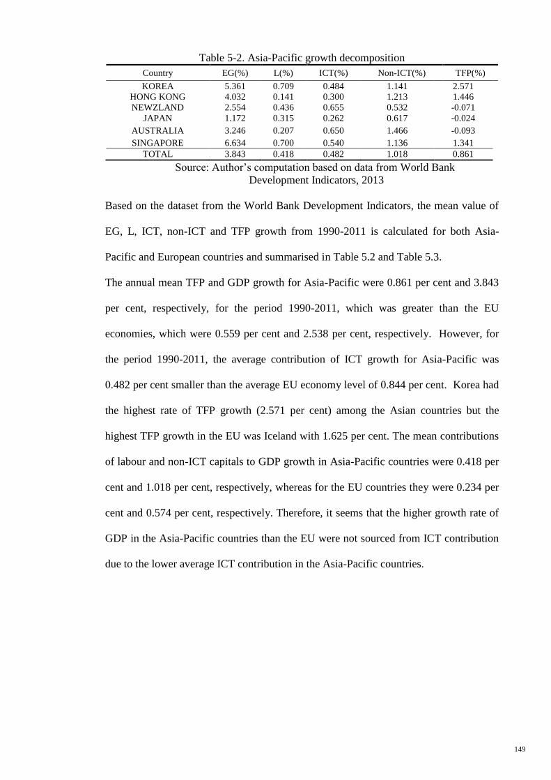
149

Table 5-2. Asia-Pacific growth decomposition

Country EG(%) L(%) ICT(%) Non-ICT(%) TFP(%)

KOREA 5.361 0.709 0.484 1.141 2.571

HONG KONG 4.032 0.141 0.300 1.213 1.446

NEWZLAND 2.554 0.436 0.655 0.532 -0.071

JAPAN 1.172 0.315 0.262 0.617 -0.024

AUSTRALIA 3.246 0.207 0.650 1.466 -0.093

SINGAPORE 6.634 0.700 0.540 1.136 1.341

TOTAL 3.843 0.418 0.482 1.018 0.861

Source: Author’s computation based on data from World Bank

Development Indicators, 2013

Based on the dataset from the World Bank Development Indicators, the mean value of

EG, L, ICT, non-ICT and TFP growth from 1990-2011 is calculated for both Asia-

Pacific and European countries and summarised in Table 5.2 and Table 5.3.

The annual mean TFP and GDP growth for Asia-Pacific were 0.861 per cent and 3.843

per cent, respectively, for the period 1990-2011, which was greater than the EU

economies, which were 0.559 per cent and 2.538 per cent, respectively. However, for

the period 1990-2011, the average contribution of ICT growth for Asia-Pacific was

0.482 per cent smaller than the average EU economy level of 0.844 per cent. Korea had

the highest rate of TFP growth (2.571 per cent) among the Asian countries but the

highest TFP growth in the EU was Iceland with 1.625 per cent. The mean contributions

of labour and non-ICT capitals to GDP growth in Asia-Pacific countries were 0.418 per

cent and 1.018 per cent, respectively, whereas for the EU countries they were 0.234 per

cent and 0.574 per cent, respectively. Therefore, it seems that the higher growth rate of

GDP in the Asia-Pacific countries than the EU were not sourced from ICT contribution

due to the lower average ICT contribution in the Asia-Pacific countries.

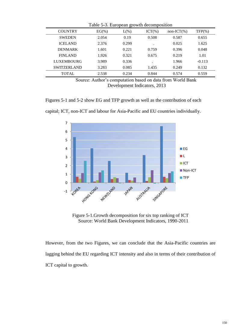
150

Table 5-3. European growth decomposition

COUNTRY EG(%) L(%) ICT(%) non-ICT(%) TFP(%)

SWEDEN 2.054 0.19 0.508 0.587 0.655

ICELAND 2.376 0.299 . 0.025 1.625

DENMARK 1.601 0.221 0.759 0.396 0.048

FINLAND 1.926 0.321 0.675 0.219 1.01

LUXEMBOURG 3.989 0.336 . 1.966 -0.113

SWITZERLAND 3.283 0.085 1.435 0.249 0.132

TOTAL 2.538 0.234 0.844 0.574 0.559

Source: Author’s computation based on data from World Bank

Development Indicators, 2013

Figures 5-1 and 5-2 show EG and TFP growth as well as the contribution of each

capital; ICT, non-ICT and labour for Asia-Pacific and EU countries individually.

Figure 5-1.Growth decomposition for six top ranking of ICT

Source: World Bank Development Indicators, 1990-2011

However, from the two Figures, we can conclude that the Asia-Pacific countries are

lagging behind the EU regarding ICT intensity and also in terms of their contribution of

ICT capital to growth.

-1

0

1

2

3

4

5

6

7

EG

L

ICT

Non-ICT

TFP

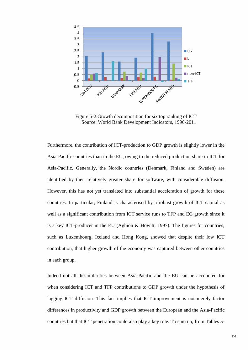
151

Figure 5-2.Growth decomposition for six top ranking of ICT

Source: World Bank Development Indicators, 1990-2011

Furthermore, the contribution of ICT-production to GDP growth is slightly lower in the

Asia-Pacific countries than in the EU, owing to the reduced production share in ICT for

Asia-Pacific. Generally, the Nordic countries (Denmark, Finland and Sweden) are

identified by their relatively greater share for software, with considerable diffusion.

However, this has not yet translated into substantial acceleration of growth for these

countries. In particular, Finland is characterised by a robust growth of ICT capital as

well as a significant contribution from ICT service runs to TFP and EG growth since it

is a key ICT-producer in the EU (Aghion & Howitt, 1997). The figures for countries,

such as Luxembourg, Iceland and Hong Kong, showed that despite their low ICT

contribution, that higher growth of the economy was captured between other countries

in each group.

Indeed not all dissimilarities between Asia-Pacific and the EU can be accounted for

when considering ICT and TFP contributions to GDP growth under the hypothesis of

lagging ICT diffusion. This fact implies that ICT improvement is not merely factor

differences in productivity and GDP growth between the European and the Asia-Pacific

countries but that ICT penetration could also play a key role. To sum up, from Tables 5-

-0.5

0

0.5

1

1.5

2

2.5

3

3.5

4

4.5

EG

L

ICT

non-ICT

TFP

152

2 and 5-3 it is apparent that ICT contribution to value added across two regional groups

is not strongly correlated with the level of GDP growth and TFP growth.

5.3 Unit Root Tests for Asia-Pacific and European Countries

Before running the cointegration approaches, we have to identify the order of

integration for each variable. One of the ways is to apply the panel unit root test of Im et

al. (2003, hereinafter IPS). This analysis is limited compared to the tests by Levin et al.

(2002) and Breitung (2000), which, usually, do not allow for heterogeneity in the

autoregressive coefficient. On the other hand, in the aggregate level, we have added

some additional variables to our model for more control. The first generation tests, such

as Levin et al. (2002), Breitung (2000) and Hardi (2000), need to be tested on strongly

balanced panels whereas the additional controlling variables in our new panels are not

strongly balanced.

Nevertheless, the test suggested by IPS resolves Levin and Lin’s serial correlation issue

by presuming heterogeneity between units in a dynamic panel framework. The IPS test

has the disadvantage of assuming that the cross-sections are independent. The equal

assumption is done in all first-generation panel unit root tests. However, it is often

mentioned in the literature that cross-section dependency may develop due to

unobserved common factors, externalities, regional and macroeconomic linkages and

unaccounted residual interdependence. Currently, the new panel unit root test presented

by Pesaran (2007) has corrected the question of the dependency and correlation

providing the prevalence of macroeconomic dynamics and linkages Therefore, we

employed the IPS (1997), Fisher-type (1999) and Pesaran (2007) tests for the two

regional group panels.

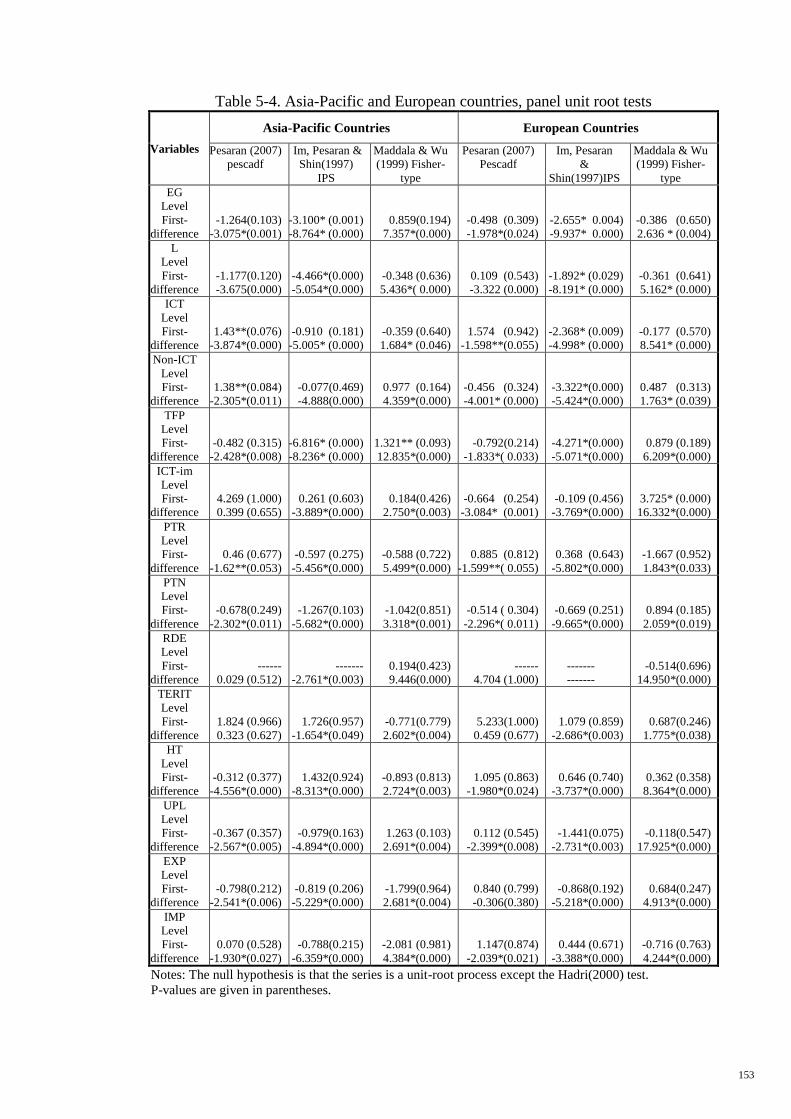
153

Table 5-4. Asia-Pacific and European countries, panel unit root tests

Variables

Asia-Pacific Countries European Countries

Pesaran (2007)

pescadf

Im, Pesaran &

Shin(1997)

IPS

Maddala & Wu

(1999) Fisher-

type

Pesaran (2007)

Pescadf

Im, Pesaran

&

Shin(1997)IPS

Maddala & Wu

(1999) Fisher-

type

EG

Level

First-

difference

-1.264(0.103)

-3.075*(0.001)

-3.100* (0.001)

-8.764* (0.000)

0.859(0.194)

7.357*(0.000)

-0.498 (0.309)

-1.978*(0.024)

-2.655* 0.004)

-9.937* 0.000)

-0.386 (0.650)

2.636 * (0.004)

L

Level

First-

difference

-1.177(0.120)

-3.675(0.000)

-4.466*(0.000)

-5.054*(0.000)

-0.348 (0.636)

5.436*( 0.000)

0.109 (0.543)

-3.322 (0.000)

-1.892* (0.029)

-8.191* (0.000)

-0.361 (0.641)

5.162* (0.000)

ICT

Level

First-

difference

1.43**(0.076)

-3.874*(0.000)

-0.910 (0.181)

-5.005* (0.000)

-0.359 (0.640)

1.684* (0.046)

1.574 (0.942)

-1.598**(0.055)

-2.368* (0.009)

-4.998* (0.000)

-0.177 (0.570)

8.541* (0.000)

Non-ICT

Level

First-

difference

1.38**(0.084)

-2.305*(0.011)

-0.077(0.469)

-4.888(0.000)

0.977 (0.164)

4.359*(0.000)

-0.456 (0.324)

-4.001* (0.000)

-3.322*(0.000)

-5.424*(0.000)

0.487 (0.313)

1.763* (0.039)

TFP

Level

First-

difference

-0.482 (0.315)

-2.428*(0.008)

-6.816* (0.000)

-8.236* (0.000)

1.321** (0.093)

12.835*(0.000)

-0.792(0.214)

-1.833*( 0.033)

-4.271*(0.000)

-5.071*(0.000)

0.879 (0.189)

6.209*(0.000)

ICT-im

Level

First-

difference

4.269 (1.000)

0.399 (0.655)

0.261 (0.603)

-3.889*(0.000)

0.184(0.426)

2.750*(0.003)

-0.664 (0.254)

-3.084* (0.001)

-0.109 (0.456)

-3.769*(0.000)

3.725* (0.000)

16.332*(0.000)

PTR

Level

First-

difference

0.46 (0.677)

-1.62**(0.053)

-0.597 (0.275)

-5.456*(0.000)

-0.588 (0.722)

5.499*(0.000)

0.885 (0.812)

-1.599**( 0.055)

0.368 (0.643)

-5.802*(0.000)

-1.667 (0.952)

1.843*(0.033)

PTN

Level

First-

difference

-0.678(0.249)

-2.302*(0.011)

-1.267(0.103)

-5.682*(0.000)

-1.042(0.851)

3.318*(0.001)

-0.514 ( 0.304)

-2.296*( 0.011)

-0.669 (0.251)

-9.665*(0.000)

0.894 (0.185)

2.059*(0.019)

RDE

Level

First-

difference

------

0.029 (0.512)

-------

-2.761*(0.003)

0.194(0.423)

9.446(0.000)

------

4.704 (1.000)

-------

-------

-0.514(0.696)

14.950*(0.000)

TERIT

Level

First-

difference

1.824 (0.966)

0.323 (0.627)

1.726(0.957)

-1.654*(0.049)

-0.771(0.779)

2.602*(0.004)

5.233(1.000)

0.459 (0.677)

1.079 (0.859)

-2.686*(0.003)

0.687(0.246)

1.775*(0.038)

HT

Level

First-

difference

-0.312 (0.377)

-4.556*(0.000)

1.432(0.924)

-8.313*(0.000)

-0.893 (0.813)

2.724*(0.003)

1.095 (0.863)

-1.980*(0.024)

0.646 (0.740)

-3.737*(0.000)

0.362 (0.358)

8.364*(0.000)

UPL

Level

First-

difference

-0.367 (0.357)

-2.567*(0.005)

-0.979(0.163)

-4.894*(0.000)

1.263 (0.103)

2.691*(0.004)

0.112 (0.545)

-2.399*(0.008)

-1.441(0.075)

-2.731*(0.003)

-0.118(0.547)

17.925*(0.000)

EXP

Level

First-

difference

-0.798(0.212)

-2.541*(0.006)

-0.819 (0.206)

-5.229*(0.000)

-1.799(0.964)

2.681*(0.004)

0.840 (0.799)

-0.306(0.380)

-0.868(0.192)

-5.218*(0.000)

0.684(0.247)

4.913*(0.000)

IMP

Level

First-

difference

0.070 (0.528)

-1.930*(0.027)

-0.788(0.215)

-6.359*(0.000)

-2.081 (0.981)

4.384*(0.000)

1.147(0.874)

-2.039*(0.021)

0.444 (0.671)

-3.388*(0.000)

-0.716 (0.763)

4.244*(0.000)

Notes: The null hypothesis is that the series is a unit-root process except the Hadri(2000) test.


154






Source: Author’s calculation, 2013

The ‘first generation’ of panel data integration tests, such as IPS (2003) and Fisher

(1999), assume cross-sectional independence among panel units (except for common

time effects), while the ‘‘second-generation’’ of panel data unit root tests, such as

Pesaran (2007), control for common time effects as well as more general forms of cross-

sectional dependency. The results of the Fisher-type (1999), IPS (2003) and Pesaran

(2007) panel unit root tests are presented in Tables 4-5 for both the Asia-Pacific and EU

countries. For all fourteen variables, the null hypotheses of the unit roots is not rejected

at level. These outcomes robustly indicate that all the variables are non-stationary in

level but become stationary in first-differences at the 10 per cent and 5 per cent

significance levels.

5.4 Panel Cointegration Tests for Asia-Pacific and European Countries

As indicated, the fundamental idea behind cointegration is to examine whether linear

combinations of variables are individually non-stationary or stationary. The Kao (1999)

residual based test was used to perform ADF stationary test on the residuals of the first

estimated model with all variables. There is a restriction for the number of variables to

handle the Pedroni (2004) cointegrating test. Therefore, in this research, we will only

employ the Kao (1999) cointegration test for the two regional groups of countries. Table

5-5 presents the Kao (1999) test results.

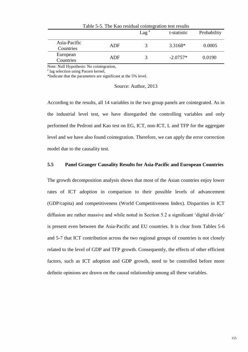
155

Table 5-5. The Kao residual cointegration test results


Asia-Pacific

Countries ADF 3 3.3168* 0.0005

European

Countries ADF 3 -2.0757* 0.0190





According to the results, all 14 variables in the two group panels are cointegrated. As in

the industrial level test, we have disregarded the controlling variables and only

performed the Pedroni and Kao test on EG, ICT, non-ICT, L and TFP for the aggregate

level and we have also found cointegration. Therefore, we can apply the error correction

model due to the causality test.

5.5 Panel Granger Causality Results for Asia-Pacific and European Countries

The growth decomposition analysis shows that most of the Asian countries enjoy lower

rates of ICT adoption in comparison to their possible levels of advancement

(GDP/capita) and competitiveness (World Competitiveness Index). Disparities in ICT

diffusion are rather massive and while noted in Section 5.2 a significant ‘digital divide’

is present even between the Asia-Pacific and EU countries. It is clear from Tables 5-6

and 5-7 that ICT contribution across the two regional groups of countries is not closely

related to the level of GDP and TFP growth. Consequently, the effects of other efficient

factors, such as ICT adoption and GDP growth, need to be controlled before more

definite opinions are drawn on the causal relationship among all these variables.

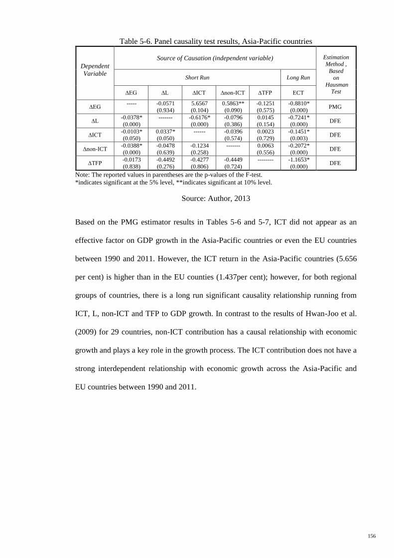
156

Table 5-6. Panel causality test results, Asia-Pacific countries

Dependent

Variable


Estimation

Method ,

Based

on

Hausman

Test

Short Run Long Run


∆EG ----- -0.0571

(0.934)

5.6567

(0.104)

0.5863**

(0.090)

-0.1251

(0.575)

-0.8810*

(0.000) PMG

∆L -0.0378*

(0.000)

-------

-0.6176*

(0.000)

-0.0796

(0.386)

0.0145

(0.154)

-0.7241*

(0.000) DFE

∆ICT -0.0103*

(0.050)

0.0337*

(0.050)

------ -0.0396

(0.574)

0.0023

(0.729)

-0.1451*

(0.003) DFE

∆non-ICT -0.0388*

(0.000)

-0.0478

(0.639)

-0.1234

(0.258)

------- 0.0063

(0.556)

-0.2072*

(0.000) DFE

∆TFP -0.0173

(0.838)

-0.4492

(0.276)

-0.4277

(0.806)

-0.4449

(0.724)

-------- -1.1653*

(0.000) DFE


*indicates significant at the 5% level, **indicates significant at 10% level.


Based on the PMG estimator results in Tables 5-6 and 5-7, ICT did not appear as an

effective factor on GDP growth in the Asia-Pacific countries or even the EU countries

between 1990 and 2011. However, the ICT return in the Asia-Pacific countries (5.656

per cent) is higher than in the EU counties (1.437per cent); however, for both regional

groups of countries, there is a long run significant causality relationship running from

ICT, L, non-ICT and TFP to GDP growth. In contrast to the results of Hwan-Joo et al.

(2009) for 29 countries, non-ICT contribution has a causal relationship with economic

growth and plays a key role in the growth process. The ICT contribution does not have a

strong interdependent relationship with economic growth across the Asia-Pacific and

EU countries between 1990 and 2011.

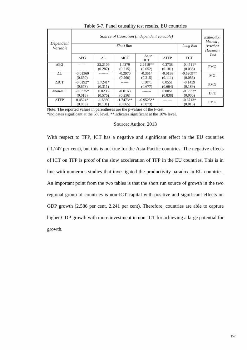
157

Table 5-7. Panel causality test results, EU countries

Dependent

Variable


Estimation

Method ,

Based on

Hausman

Test

Short Run Long Run

∆EG ∆L ∆ICT ∆non-

ICT ∆TFP ECT

∆EG ----- 22.2106

(0.287)

1.4379

(0.215)

2.2419**

(0.052)

0.3738

(0.181)

-0.4511*

(0.036) PMG

∆L -0.01360

(0.630)

-------

-0.2970

(0.260)

-0.3514

(0.215)

-0.0198

(0.111)

-0.5209**

(0.086) MG

∆ICT -0.0192*

(0.673)

3.7241*

(0.311)

------ 0.3071

(0.677)

0.0551

(0.664)

-0.1439

(0.189) PMG

∆non-ICT -0.0335*

(0.018)

0.0235

(0.575)

-0.0168

(0.256)

------- 0.0051

(0.838)

-0.3332*

(0.000) DFE

∆TFP 0.4524*

(0.003)

-1.6360

(0.131)

-1.7473**

(0.065)

-0.9525**

(0.073)

-------- -0.3713*

(0.016) PMG




With respect to TFP, ICT has a negative and significant effect in the EU countries

(-1.747 per cent), but this is not true for the Asia-Pacific countries. The negative effects

of ICT on TFP is proof of the slow acceleration of TFP in the EU countries. This is in

line with numerous studies that investigated the productivity paradox in EU countries.

An important point from the two tables is that the short run source of growth in the two

regional group of countries is non-ICT capital with positive and significant effects on

GDP growth (2.586 per cent, 2.241 per cent). Therefore, countries are able to capture

higher GDP growth with more investment in non-ICT for achieving a large potential for

growth.

158

Table 5-8. Panel industries direction of causality in short run and long run, Asia-Pacific




Table 5-8 shows long run bidirectional causality between GDP growth and contribution

of ICT, L, non-ICT and TFP growth for Asia-Pacific countries, while there is only

unidirectional causality running from ICT to GDP and TFP growth in the EU panel.

For EU countries in the short run, there is no causality relationship between ICT capital

and GDP growth, but, for the Asia-Pacific countries, unidirectional causality runs from

economic growth to ICT contribution. Therefore, short run ICT investment policies do

not have any impact on growth for the two regional groups of countries; it needs to

switch to long run ICT investment policies for both Asia Pacific and the EU. Indeed, in

the short run, the high growth rate of GDP in countries like Singapore and Korea

increases the ICT spillover effects on TFP to sustain economic growth.

Short run causality Long run causality Direction of Causality Wald F-test Direction of Causality Wald F-test

∆EG -------- ∆L

(0.507)

(0.000)*

EG ------ L

(0.000)*

(0.000)*

∆EG -------- ∆ICT (0.001)*

(0.050)* EG ------ ICT

(0.000)*

(0.003)*

∆EG ------ ∆non-ICT (0.012)*

(0.000)* EG ------ non-ICT

(0.000)*

(0.000)*

∆EG No causality ∆TFP (0.280)

(0.838) EG ------ TFP

(0.000)*

(0.000)*

∆L ------ ∆ICT

(0.000)*

(0.050)*

L ------ ICT

(0.000)*

(0.003)*

∆L No causality ∆non-ICT

(0.386)

(0.639)

L ------ non-ICT

(0.000)*

(0.000)*

∆L No causality ∆TFP

(0.154)

(0.276)

L ------ TFP

(0.000)*

(0.000)*

∆ICT No causality ∆non-ICT

(0.574)

(0.258)

ICT ------ non-ICT

(0.000)*

(0.003)*

∆ICT No causality ∆TFP (0.729)

(0.806)

ICT ------ TFP

(0.000)*

(0.003)*

∆non-ICT No causality ∆TFP (0.724)

(0.556) non-ICT ------ TFP

(0.000)*

(0.000)*

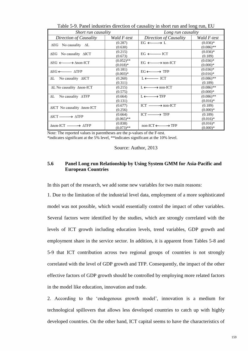
159

Table 5-9. Panel industries direction of causality in short run and long run, EU




5.6 Panel Long run Relationship by Using System GMM for Asia-Pacific and

European Countries

In this part of the research, we add some new variables for two main reasons:

1. Due to the limitation of the industrial level data, employment of a more sophisticated

model was not possible, which would essentially control the impact of other variables.

Several factors were identified by the studies, which are strongly correlated with the

levels of ICT growth including education levels, trend variables, GDP growth and

employment share in the service sector. In addition, it is apparent from Tables 5-8 and

5-9 that ICT contribution across two regional groups of countries is not strongly

correlated with the level of GDP growth and TFP. Consequently, the impact of the other

effective factors of GDP growth should be controlled by employing more related factors

in the model like education, innovation and trade.

2. According to the ‘endogenous growth model’, innovation is a medium for

technological spillovers that allows less developed countries to catch up with highly

developed countries. On the other hand, ICT capital seems to have the characteristics of

Short run causality Long run causality Direction of Causality Wald F-test Direction of Causality Wald F-test

∆EG No causality ∆L (0.287)

(0.630)

EG ------ L

(0.036)*

(0.086)**

∆EG No causality ∆ICT (0.215)

(0.673) EG -------- ICT

(0.036)*

(0.189)

∆EG ------ ∆non-ICT (0.052)**

(0.018)* EG ------ non-ICT

(0.036)*

(0.000)*

∆EG -------- ∆TFP (0.181)

(0.003)* EG ------ TFP

(0.036)*

(0.016)*

∆L No causality ∆ICT

(0.260)

(0.311)

L -------- ICT

(0.086)**

(0.189)

∆L No causality ∆non-ICT

(0.215)

(0.575)

L ------ non-ICT

(0.086)**

(0.000)*

∆L No causality ∆TFP

(0.664)

(0.131)

L ------ TFP

(0.086)**

(0.016)*

∆ICT No causality ∆non-ICT (0.677)

(0.256)

ICT -------- non-ICT

(0.189)

(0.000)*

∆ICT -------- ∆TFP (0.664)

(0.065)**

ICT -------- TFP

(0.189)

(0.016)*

∆non-ICT -------- ∆TFP (0.838)

(0.073)** non-ICT ------ TFP

(0.016)*

(0.000)*

160

both forms of capital, traditional forms of capital as a production technology and

knowledge capital in its informational nature (Dedrick, Gurbaxani, & Kraemer, 2003).

An essential characteristic of the debate under the existence of ICT spillover is whether

the ICT capital stock may also boost economic growth through positive spillover effects

on TFP, if ICT capital is like knowledge capital. The sources for total factor

productivity (TFP) growth may be relatively different over time and across countries,

but technological change and innovation have been mainly acknowledged as

determinants of TFP growth, and ICT has been considered as the major form of

technological change in recent decades (Madden & Savage, 2000). Thus, if we add new

variables that are related to the spillover effects of ICT, the significance of the model

should increase.

The descriptive list of variables, which is using the estimation in the long run model,

has been mentioned in Table 1 of the study. Moreover, it should be remembered that

GMM estimators are particularly practical for panel data with comparatively small time

length (T), in comparison to the number (N) of cross-sections (Roodman, 2006). In

contrast, as T becomes larger, misleading and inconsistent coefficient estimates could

be produced by the GMM estimator unless and until the slope coefficients are the same

throughout the cross-sections (Pesaran & Smith, 1995). Through the estimation of

separate regression of two time groups, the problem of a relatively large time dimension

(N = 26, T = 21) has been addressed for the sub-periods of 1980-1990 and 1990-2000.

As justified, it has enabled us to search for the varying effects of ICTs across time.

Furthermore, the start and end points of the periods have been selected in such a way

that the economy is at similar stages of the business cycle. This has been preferred due

to the elimination of the impact of business cyclical factors on the output measures.

In this research, System GMM is selected in the industrial level panel and first-

difference GMM for the aggregate level. However, a couple of crucial issues need to be

161

addressed regarding employing System GMM. First, since System GMM uses added

instruments compared to the difference GMM it might not be proper to apply System

GMM with a dataset comprising a small number of countries (Mileva, 2007). From the

methodology part, aggregate panel data are estimated across six countries (N=6) in 11

sub periods (T=11) for each group of countries. Therefore, we are going to use first-

difference GMM for the aggregate level part due to the small number of countries and

System GMM for the industrial level part with large cross-sectional data (N=21, T=17).

Arrelano and Bond (1991) GMM regressions are carried out based on equation (15),

after applying the heteroscedasticity robust one-step estimator, while setting out

individual regressions for both groups of Asia-Pacific and EU countries. Table 5-10

presents the estimation outputs for the sample of the Asia-Pacific and EU countries

individually per decade (columns 1 and 2, 3 and 4). In the columns for the two regions,

we intend to verify the differential impacts before and after 2000 to estimate the greater

ICT growth contribution in the United States between 1996 and 1999 and we need to

test whether it supports the Asia-Pacific and EU panels.

From the presented estimates of Table 5-10, it appears that the effects of non-ICT on the

Asia-Pacific countries growth were highly positive and significant over two periods,

while employment capital seems to be correlated negatively and significantly with

output growth. Similar estimation results are reported for the EU (columns 3, 4); both L

and non-ICT were highly positive and significant over two periods, with the exception

of the first period for non-ICT capital, the impact of which reduces.

TFP growth has emerged as having a significant and positive effect on GDP growth for

both regions during the two periods with a difference in magnitude that shows that the

positive effect for Asia-Pacific countries in the second period is higher than its first

period but for the EU, the growth of TFP in the first period is more effective for GDP

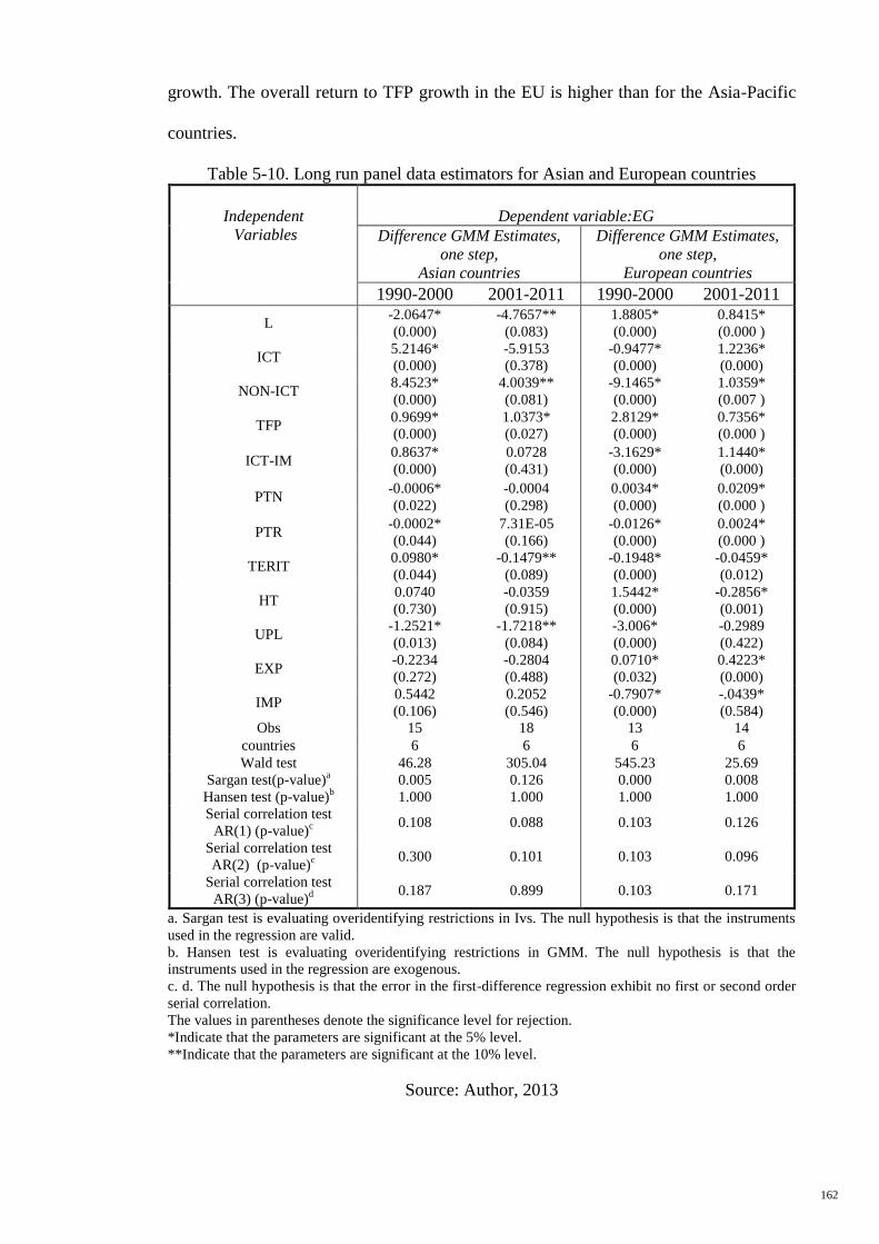
162

growth. The overall return to TFP growth in the EU is higher than for the Asia-Pacific

countries.

Table 5-10. Long run panel data estimators for Asian and European countries

Independent Variables


Difference GMM Estimates, one step,

Asian countries

Difference GMM Estimates, one step,

European countries

1990-2000 2001-2011 1990-2000 2001-2011

L -2.0647*

(0.000)

-4.7657**

(0.083)

1.8805*

(0.000)

0.8415*

(0.000 )

ICT 5.2146*

(0.000)

-5.9153

(0.378)

-0.9477*

(0.000)

1.2236*

(0.000)

NON-ICT 8.4523*

(0.000)

4.0039**

(0.081)

-9.1465*

(0.000)

1.0359*

(0.007 )

TFP 0.9699*

(0.000)

1.0373*

(0.027)

2.8129*

(0.000)

0.7356*

(0.000 )

ICT-IM 0.8637*

(0.000)

0.0728

(0.431)

-3.1629*

(0.000)

1.1440*

(0.000)

PTN -0.0006*

(0.022)

-0.0004

(0.298)

0.0034*

(0.000)

0.0209*

(0.000 )

PTR -0.0002*

(0.044)

7.31E-05

(0.166)

-0.0126*

(0.000)

0.0024*

(0.000 )

TERIT 0.0980*

(0.044)

-0.1479**

(0.089)

-0.1948*

(0.000)

-0.0459*

(0.012)

HT 0.0740

(0.730)

-0.0359

(0.915)

1.5442*

(0.000)

-0.2856*

(0.001)

UPL -1.2521*

(0.013)

-1.7218**

(0.084)

-3.006*

(0.000)

-0.2989

(0.422)

EXP -0.2234

(0.272)

-0.2804

(0.488)

0.0710*

(0.032)

0.4223*

(0.000)

IMP 0.5442

(0.106)

0.2052

(0.546)

-0.7907*

(0.000)

-.0439*

(0.584)

Obs 15 18 13 14

countries 6 6 6 6

Wald test 46.28 305.04 545.23 25.69




AR(1) (p-value)c

0.108 0.088 0.103 0.126


AR(2) (p-value)c

0.300 0.101 0.103 0.096


AR(3) (p-value)d

0.187 0.899 0.103 0.171






serial correlation.





163

The ICT growth impact only seems to have increased significantly in magnitude during

the 1990s and 2000s for the EU countries. While in the Asia-Pacific countries, ICT lost

effect in both magnitude and significance on GDP growth during the 2000s. This can be

interpreted as ICT was the engine of growth in the 1990s for the Asia-Pacific countries,

whereas it had the same role in growth for the EU economy in most cases through to the

2000s.

According to the Asia-Pacific results, for 1990-2000, the ICT effect increased

considerably, presenting a highly positive and significant relationship with output

growth that was experienced in the second part of 1995. This proof demonstrates the

stylised facts shown in the literature, that the ICT growth contribution was enhanced

extensively throughout 1995, especially in Asia, similar to the US economy but unlike

the EU countries.

Regarding the EU industries, the total ICT growth contribution is significant in the two

periods (columns 3 and 4). In the 2000s, its effect is substantially increased in

magnitude and significance compared to 1990-2000. All this information shows that

ICT should be able to play a significant role in improving growth among the EU

countries, via its speedier capital accumulation. In spite of this, the pertinent worth of

ICT increased significantly through the second period from -0.94 to 1.22, whereas for

Asia-Pacific it dropped from 5.214 to -5.915. In general, it seems that when comparing

the results of two regional groups of countries, the impact of ICT is higher in the EU

economy than for the Asia-Pacific countries not only from the direct effects of ICT as

capital but also through TFP growth by positive spillover effects.

Considering the other explanatory variables for controlling the spillover effects of ICT

independently from TFP, it is interesting to know that most of them are only robustly

significant in the EU and Asia-Pacific countries during the first period. For example, the

coefficient of patent application for residents and non-residents and school enrolment

164

(PTN, PTR, TERIT) are statistically significant at the 5% significance level in columns

(1) and (3) but PTR and PTN are insignificant for the second period of Asia-Pacific

countries. In addition, the magnitude of this coefficient is higher in the first period for

Asia-Pacific but it is higher in the second period in the EU countries. The significance

of the education and patent variables suggest that educational and patent attainments are

important determinants of the ICT contribution to growth. The coefficient is negative

but higher in the EU than Asia-Pacific, which suggests that the impact of education and

patent application were somewhat accelerated and more effective in the EU economies

Similar patterns are also observed for unemployment, ICT import and high-technology

export and import goods and services (UPL, ICT-IM, HT, EXP, and IMP). HT, EXP,

and IMP are totally insignificant for the Asia-Pacific countries while they have

significant effects in the EU for both periods together with the expected signs. Since the

signs for the variables for the Asia-Pacific countries are not as expected in the findings,

one should bear in mind the drawback of the variables of export and import, which did

not adequately capture the openness of the Asia-Pacific economies. The outcomes

indicate that the openness provides some negative effect on ICT contribution to output

growth. However, this effect is not statistically significant.

The unemployment rate has a negative and significant impact on growth for the two

regional groups of countries except for the second period of the EU economies. ICT

imports emerged as a significant factor for all the countries except the second period for

the Asia-Pacific countries. The results suggest that education, openness and high quality

patents are supposed to be among the main determining factors of the difference in ICT

spillover impacts to output growth across economies. Along with these elements, it is

predicted that ICT and technology trade is usually an essential determinant of the ICT

spillover impact on growth because countries with a higher level of trade may gain large

benefits from the Internet, for which online trade is the dominant way of export and

165

import (Vu, 2005). Furthermore, it is shown that knowledge spillovers have been an

important contributing factor behind the TFP convergence among the countries over the

whole period. Knowledge spillovers from ICT use in education to ICT use somewhere

else, provide several fields for policy involvement by developing the ‘effective

computer literacy spillover potential’ of proper education, thereby positively affecting

the overall growth performance.

To sum up, it seems that the spillover effects of ICT between 1990 and 2000 emerged

more than between 2001 and 2011 and more strongly in the EU than for Asia-Pacific

countries over two decades. Most of these results expressed that boosting these main

determinants is an efficient method to foster ICT diffusion and its effect on economic

growth.

As mentioned in the earlier sections, the constancy of the GMM estimator is dependent

on the validity of the instruments employed in the GMM regression along with the

absence of the second-order serial correlation in the error term. Table 5-10 documents

the outputs of the Hansen J test and of the second and third order serial correlation test.

For all of the conditions, the Hansen J test does not reject the null hypothesis that the

instruments applied in the regressions are valid. Moreover, the test that checks for serial

correlation does not reject its null hypothesis, indicating that the error term fails to

manifest serial correlation in the first and second order correlation.

5.7 Justification of insignificant effects of ICT on GDP growth in EU and

Asia-Pacific countries

Tables 5-6 and 5-7 present the results for the EU and Asia-Pacific countries,

respectively. It is indicated in the Hausman test that proof of the equality among the

PMG, DFE and MG estimates is not rejected and it is shown that common long run

elasticity is accepted by the data. Consequently, our estimated results are based on the

166

PMG estimators, which are estimated as maximum likelihood, while the Schwartz

Bayesian Criterion is used to choose the appropriate lag length.

The Asia-Pacific econometric results are reported in the first row of Table 5-6. With

respect to the ICT impact on output growth, we can see that the estimated short run

effect for the period 1990-2011 is positive and insignificant. Particularly, the

implication of its magnitude is that an increase of 1 per cent in ICT capital increases the

output growth by 5.66 per cent. As compared to the System GMM estimates, the

reported long run coefficient’s magnitude is comparatively more. The insignificant

effect of ICT on GDP growth is positive in 1990-2000 and negative in 2001-2011 for

Asia-Pacific, which is inverse to that of the EU, and which may have different reasons

listed as follows:

1. In the GMM results, we noticed that the ICT capital’s impact is insignificantly

negative between 2001 and 2011. One of the most important criteria of ICT in society is

rapid progress and development during the short-term. In theory, while a new severe

innovation, such as new equipment of ICT arrives, economies suffer from primary

economic loss; consequently, it emerges in a kind of capital obsolescence that would

decrease GDP growth (Helpman & Trajtenberg, 1998; Aghion & Howitt, 1998).

2. Empirically, evidence has been presented in previous research regarding the declining

effect of ICT capital on productivity in the economy. The negative long run impact of

ICT capital is quite doubtful, so this finding is attributed to factors related to parameter

heterogeneity throughout countries and model uncertainty, or certain outlier impacts

that are currently considered as the main constraints in the modern empirical growth

literature (Striroh, 2002).

3. Similar ambiguities could be found in the GMM results. For instance, with regards to

FDI (Foreign Direct Investment), it is shown by Blomstrom et al. (1996) that there is a

decrease in the significance of the fixed investment variable when total capital is split to

167

non-FDI and FDI investment. Therefore, in this research, the capital factor is divided

into non-ICT and ICT capital. It could be possible that the qualitative nature of other

forms of capital, similar to ICT, is more impressive than the common augmentation of

fixed capital stocks. It can be pointed out that during the 2000s, the importance of non-

ICT capital declines when the total capital is distributed in non-ICT and ICT for EU and

Asia-Pacific countries. This interpretation can be true for the PMG results for Asia-

Pacific countries as well.

4. Despite the insignificant effects of ICT in the short run findings reported by PMG for

both periods, the overall contribution of ICT on growth is significant and positive

(columns 3 and 4) in EU countries. In the 2000s, as compared to the 1990s, there seems

to be a substantial increase in the magnitude of its impact and the sign is also changed to

positive. It is suggested by the results that through faster accumulation of capital, ICT

can have a pivotal role in the enhancement of growth amongst the member countries of

the EU. During the 2000s, there was a significant drop in the relative importance of ICT

in the Asia-Pacific countries (column 2), while it increased from -0.94 to 1.22 in the

EU. Generally, when the results of Tables 5-10 are compared, the impact of ICT is

lower in the economy of the EU relative to the economy of Asia-Pacific, an outcome

that was discussed in Section 5.6 and presented as a stylized fact.

5. In Asia-Pacific countries, such as Japan and Korea, during the 1990s a burst of

productivity in the industries producing ICT equipment (computer hardware, software

and telecommunications) led to a fall in the relative prices of ICTs, thereby increasing

investment in ICT assets and capital-deepening across the whole economy. Therefore,

ICT had a considerably significant and positive effect on the EG during the 1990s. In

contrast, most of the literature attributes the European slow-down in productivity

growth to the lag in ICT adoption by the ICT-using sector after 1995. Factors related to

168

national regulations may play a role in explaining the slow reorganisation of European

firms around the new technology.

6. After 2007, the economic crisis drew a different picture in the Asia-Pacific and EU

economies, with negative rates of GDP growth in both Asia-Pacific and the European

countries. The average drop in GDP in the EU was slower than for the Asia-Pacific

countries; thus, in the Asia-Pacific economies, adjustment to the crisis mainly occurred

in the TFP and resulted in a dramatic decrease in the ICT-producing sector, whereas, in

Europe, TFP losses were smaller and the adjustment occurred through a decrease in

labour productivity. Nevertheless, labour quality and ICT investment continued to

provide a positive contribution to growth (Van Ark, 2010).

7. The findings in this research suggest that the Asia-Pacific countries might benefit

more from ICT than the countries in Europe. The GMM results revealed significant and

positive returns from ICT capital that were larger in magnitude for the Asia-Pacific

countries than the EU countries in the given sample. In this study, this gap is attributed

to the absence of complementary investment as well as the low level of ICT investment

in the Asia-Pacific countries. To obtain the productivity from ICT investment,

complementary investment is a prerequisite, which includes knowledge-based

structures, human capital and infrastructure, which, although available in the EU, are

mostly unavailable in developing countries. Therefore, according to the causality

findings of the research, economic growth is one of the sources of increasing ICT in

these countries.

8. Complementary investments in countries have played an important role in reaping the

full benefits of ICT. After sufficient complementary investments are developed, the new

GPT spreads among the sectors, and, as such, the economy passes through the

productivity paradox phase in which output growth and TFP accelerates. Furthermore,

there is an argument that during the initial stage a creative destruction pattern emerges,

169

in which an initial fall in the growth of the GDP can be caused by capital obsolescence.

In particular, if it were assumed that technological change is brought about by a rapid

rate of capital, this would bring about the deskilling of human capital and the rapid rate

of capital obsolescence, which, in turn, would lower the growth of GDP.

With regards to the EU results, the PMG long run estimators confirm the results of the

System GMM estimates, which are reported in Table 5-10. In the short run, ICT’s

impact on output growth is insignificant and positive. For the EU, it seems that the

significance and magnitude of the long run impact of ICT is lower relative to Asia-

Pacific. This evidence is in line with the theoretical prediction, which states that there is

an expectation of time lag in the effects of ICT. Consequently, the countries that lead in

the implementation of ICT technology are expected to have higher returns from ICT.

This means that the adoption of ICT technology in the EU takes a longer time than in

the Asia-Pacific countries

In the 2000s, the impact of ICT was considerable, which indicates a significant and a

highly positive relationship with the growth of output, which is essentially understood

from the GMM results for the EU. This proof settles the stylized facts in Table 5-10 and

discussed in Section 5.6, in that there was substantial improvement in the growth

contribution of ICT during the second period of the EU economy.

All four Asian Dragons – Taiwan, Hong Kong, South Korea and Singapore – heavily

invested in the sector of telecommunications, and, consequently, earned enormous

benefits in the form of increasing exports. The Japanese pattern was not followed by

them, instead, a better developmental model was found, which was appropriate for their

particular economic requirements. Their economies were opened up to foreign

participation by way of promoting the transfer of technology and using it to their

maximum advantage for the formation of skills. In detail, the achievement of these

countries has brought about a change in global production trends, such as a high

170

percentage of ICT-production in terms of semiconductors, which are currently

manufactured on their shores. Many niches have been established by the electronic

products of NIEs in the global markets through their own technological progress.

Although they are not a major threat to the American and Japanese ICT companies

(excluding the field of semiconductors) due to the absence of substantial investment in

research and development for simple sciences and also because of the shortage in

capital, they persistently sell considerably well in a globalized world.

In recent months, other than South Korea, all the other Asian Dragons have

demonstrated their capability of eluding the worst part of the financial crises that has

gripped most of the Asia-Pacific region. Initial signs of recovery in South Korea, have

already started to become apparent as foreign investors have again started to pour

capital into the South Korean economy. For instance, despite the emerging competition,

with US$40 billion market capitalisation, SingTel is the most efficient

telecommunication company in Asia.

South Korea was connected to the liberalisation bandwagon from 1991, as it recognised

that market and technological externalities attract foreign investors and benefit the

corporate sector. This is because, in 1991, there was a change in South Korea’s

Telecommunications Business Law for the privatisation of its PTT, which is now

known as Korea Telecom (KT). Korea’s mobile communications sector was also

privatised to form Korea Mobile Telecommunications, and, after further

commercialisation, it became SKT Mobile. Korea has produced new innovations in the

telecommunications sector with the invention of CDMA by Samsung for cellular

telephones.Hong Kong’s cellular telephone sector has a continuous growth at 15 per

cent annually with cellular services enjoying a high penetration rate. Historically, Hong

Kong’s principal supplier of equipment produces Cable and Wireless (C&W) services.

171

To summarise, the above reasons demonstrate that the continued privatisation and

liberalisation in the Asian Dragon’s telecommunications sector will ensure that, despite

the global economic crisis, continuous ICT convergence will be experienced by these

countries as a powerful force in their continuous development.

172

6 CHAPTER 6: CONCLUSION, POLICY IMPLICATIONS, AND

FURTHER RESEARCH

6.1 Introduction

The accumulation of Information Communication Technology (ICT) capital having a

positive influence on the productivity growth and rising income in various countries has

attracted much debate among economists in recent years.

On the one hand, it is claimed that the improvement of ICT has a positive short-lived

effect but no long run effect on growth. On the other hand, it is argued that ICT has

provided important changes in the economy due to durable developments in growth

prediction. ICT is a sort of technology with wide access to numerous parts and has

supplied complementary goods and services to further enhance productivity through

specialisation and economies of scale.

Empirical analysis of economic growth and productivity has brought to light three

distinct effects of ICT. First, ICT has attracted investment, which, in itself, has

contributed to capital deepening, and, as such, helped in raising productivity and growth

in Gross Domestic Product (GDP). Second, rapid technological progress in the

production of ICT goods and services has also contributed to the growth in the

efficiency of capital and labour. This also means that total factor productivity (TFP) in

the ICT-producing sector brings greater returns to the ICT-producing sector. Third,

greater use of ICT in the economy can help business firms in the enhancement of their

overall efficiency. This means that increasing TFP may bring higher returns to ICT-

using sectors.

The review of ICT literature has proved that, since 1990, ICT diffusion in Europe has

followed a different pattern relative to Asian countries. These differences may start with

a quick improvement of computing equipment in offices, which is followed by a surge

173

in communication equipment, thus increasing investment in software services,

particularly in such Asian countries like Japan and Korea. The ICT development

ranking of countries was overlooked in the discussion of the ICT effects. For these

reasons, we have covered the above three effects of ICT on the economic growth of 12

top ranked ICT developed countries in Asia-Pacific and the European zone over the

period 1990 to 2011. This study also finds differences in country performances in the

two regions.

This study has identified the causal relationship between the contribution made by ICT

and TFP to economic growth by using panel data for 12 Asia-Pacific and European

countries over the period 1990 to 2011. Furthermore, ICT has played different growth

roles in the form of ICT-producing and ICT-using industries over 1990 to 2007. We

have also examined the long-term impact of ICT and capture the long run equilibrium

relationship among GDP growth, contribution of ICT and non-ICT labour force, TFP

and other variables. Our main findings can be classified into two major results. First,

and indeed the main result, relates to the industrial level data of countries like Japan,

Finland, Sweden, Denmark and Australia, which considered the ICT effects on growth

of 21 industries for each country. Second, is the aggregate level data that looked at 12

ICT developed countries in Asia-Pacific and Europe.

The average ICT contribution to the economic growth in these countries has been

between 0.4 per cent and 0.5 per cent per year depending on the country. During the

1990s, the ICT contribution rose from 0.3 to 1.16 percentage points per year while

during the 2000s this contribution fluctuated between 0.23 to 0.93 percentage points per

year. Our research shows that despite the differences among countries, the EU countries

have not been alone in benefiting from the positive effects of ICT capital investment on

economic growth while they did not experience an acceleration of these effects. ICT

174

diffusion plays a key role and depends on the right framework conditions, not

necessarily on the existence of an ICT-producing sector (Colecchia & Schreyer, 2002).

6.2 Main Findings of Industrial Level Data

6.2.1 Japan

According to the growth decomposition analysis of the previous chapter, Japan suffered

economic stagnation through the last period due to three factors that played a role in the

growth slump. The deceleration in TFP accounted for 8 per cent of the sluggish

performance, whereas the negative contribution of labour and the fall in the contribution

of ICT input growth each accounted for 44 per cent and 10 per cent of the sluggish

performance, respectively. In line with the results of Fukao et al. (2009), the EU

KLEMS statistics also show in detail that the ICT contribution rate dropped by an

average of 0.26 per cent, from 0.43 per cent to 0.30 per cent from 1990 to 2007 in

Japan.

Considering the ICT effect on output growth, we notice that the estimated short run

impact for the period 1990-2007 is negative and insignificant. Notably, its magnitude

means that a 1 per cent rise in ICT capital results in a 0.098 per cent decrease in output

growth among 21 industries. In Japan, ICT is only considered as significant and positive

capital in six industries, which include transport, storage, post and telecommunication

sectors. We additionally note that the results of non-ICT capital are significantly

positive. Theoretically, whenever a highly upgraded modernisation (such as ICT)

emerges, the economy as a whole does experience preliminary economic loss (Dimelis

& Papaioannou, 2011). For this reason, we want to test the complementary hypothesis

between ICT and non-ICT capital, which includes their interaction term (ICT_non-ICT)

like a different regressor in the long run relationship. The outcomes prove that there is

no significant complementary impact between ICT and non-ICT capital. As a result, the

Japanese economy has not considered ICT as a major modernisation tool since non-ICT

175

reported a positive significant effect. In line with Helpman and Trajtenberg (1998), the

economy would have initial losses attributed to the negative significant effect of non-

ICT capital.

With respect to the TFP results, the impact of ICT on TFP is negative (-0.157) and

insignificant in the short run while non-ICT and labour are significant and negative

(0.386, -0.284). This evidence is in line with the theoretical expectation that the impact

of ICT on TFP at the industrial level is expected with a time lag but significant in the

long run. Empirically, Stiroh (2002a) provided proof of a reduction in the impact on

productivity of ICT capital in the EU economy. Similar proof has been presented by

O’Mahony and Vecchi (2005) for an industry level research that addresses the US and

United Kingdom sectors.

The causality results for Japan have been reported as negative and statistically

significant coefficients of the Error Correction Term (ECT) implying that any

divergence of output growth from the long run equilibrium level causes a change in the

opposite direction. Moreover, the long run bidirectional Granger causality is shown

running real GDP growth to the contribution of L, ICT, non-ICT, and TFP growth at the

5% significant level. Except for ICT capital, there is a bidirectional Granger causality

relationship between contribution of non-ICT, L, and TFP growth to value added

growth in the short run. As a result, contrary to Gholami (2006) and Van Ark et al.

(2003), at the aggregate level, ICT is the determinant factor for economic and TFP

growth in Japan, but only in the long run.

Evidently, the ICT contribution effect was significantly positive, and quite considerable

in the ICT-producing (2.277) relative to the ICT-using (-0.249) sectors. Moreover,

regarding the differential impacts of ICT in the ICT-producing and ICT-using

industries, the impact of ICT immediately turns into an insignificant level. We may

176

possibly conclude that the worthwhile impacts of ICT largely focused on ICT intensive

industries similar to Jorgenson et al. (2003) and Van Ark et al. (2003).

Furthermore, an insignificant ICT coefficient in the two-step System GMM results

shows that adoption of new ICT was slow and smaller than the contribution of

conventional inputs like non-ICT and labour. Japan needs to create a more conducive

environment for technological diffusion. Some areas of inadequacy may exist in the

Japanese ICT strategies to ensure a sustained period of economic growth that require

attention (Gholami, Sang-Yong, & Heshmati, 2006). Updated reports of the Japanese

economy suggest that investment in ICT could have had a negative effect on economic

growth in the short run (Japan Economic Update, 2002). According to Figure 4-2,

“Textiles, leather and footwear” industries in Japan have the highest proportion of value

added growth by an average 17% growth rate per year attributed to the other sectors,

even though these industries are neither ICT-producing nor ICT-using sectors.

Therefore, the economic growth of Japan is affected by “Textiles, leather and footwear”

as a main productive sector while ICT has an insignificant impact on this industry.

6.2.2 Sweden

In the early 1990s, the growth in productivity in the Swedish manufacturing industry

was probably the largest within the EU countries. Although it is obvious that a declining

trend in productivity growth was a global phenomenon throughout the 1990s, Sweden

responded strongly. It is a well-known fact that sustainable enhancement in the supply

of factors performs a significant role in enhancing total factor productivity. ICT with

minimum standard deviation has the least fluctuation among the effective components

of economic growth and its spillover effects through TFP contribution increased

considerably (57 per cent).

With regards to the ICT influence on industrial output growth, we are able to classify

that the estimated short run impact for the period 1990-2007 is positive and significant.

177

Particularly, its magnitude means that a 1 per cent rise in ICT capital leads to a 0.93 per

cent improvement in output growth. We also noticed that the impact of non-ICT capital

is significantly negative (-0.046). In contrast to the results for Japan, it seems that ICT

as new modern capital has been replaced by non-ICT capital in Swedish industries

because these results showed significant complementary effects between ICT and non-

ICT capital.

With respect to the dynamic fixed effect estimator results of Sweden, most cases

confirm the impact of ICT on total factor productivity as negative (-0.9801) and also

significant at the 5 per cent significant level in the short run. This proof is in line with

the theoretical foresight that the impacts of ICT are anticipated with a time lag at the

industrial level, which is in line with the results for Japan. Furthermore, it is revealed

that there is long run and short run bidirectional Granger causality among GDP growth

and contribution of ICT, non-ICT, L, and TFP growth are at the 5 per cent and 10 per

cent level, respectively. In addition, the findings indicated that there is panel short run

and long run bidirectional causality among ICT, TFP growth, non-ICT and TFP at the 5

per cent and 10 per cent significant levels.

The long run results are consistent with Dimelis and Papaioannou’s (2011) findings for

a panel of EU and US countries, as developed countries, but differ with Vu’s (2011)

findings for a panel comprising of six countries of the Gulf Cooperation Council. The

long run System GMM estimations give the impression that the TFP contributed

positively and significantly (0.963 per cent) to output growth. From the PMG estimators

finding, the overall ICT growth contribution is positive and significant. However, the

System GMM results revealed that these positive effects stemmed more from ICT-using

industries because the effects of ICT-producing industries are insignificant to value

added growth.

178

6.2.3 Australia

Australia is a country with strong TFP growth in ICT-using industries but not important

as an ICT-producing sector. For this reason, Australia recorded significant development

in ICT investment in the 1990s and achieved a considerable growth between 1990 and

2007 (0.76 per cent). The growth decomposition analysis showed a 34 per cent

contribution of ICT to the annual output growth in Australia. This is due to the quick

diffusion of ICT among companies in the 1990s to match the rapid growth in

investment. The explanation introduced in the literature, is, that in 1993-94, around 50

per cent of firms in a great number of sectors had computers and around 30 per cent had

easy Internet access. By 2000-05, these percentages had grown to nearly 85 per cent

and 70 per cent, respectively (Gretton et al., 2002).

The panel Granger causality results reported that a 1 per cent increase in ICT

contribution increases GDP by 0.41 per cent, while a 1 per cent increase in L, non-ICT,

and TFP increases the value added growth by 0.20 per cent, 0.19 per cent, and 0.19 per

cent, respectively. It is important to note that non-ICT capital has become insignificant

to GDP growth in the short run.

There is bidirectional long run causality among value added growth, contribution of

ICT, non-ICT, L, and TFP pairwise. Therefore, we could identify ICT as a major source

of growth in the Australian sectors over 1990-2007 (0. 41 per cent). In addition, ICT has

a negative and significant relationship with TFP in the short run as well as in the long

run. The findings indicated that there is unidirectional short run panel Granger causality

running from EG, labour capital and TFP to non-ICT. This means that non-ICT in

Australia might not be the determining factor of output and TFP growth in the short run.

To sum up, all the results of causality evidence are in line with the Swedish industrial

results.

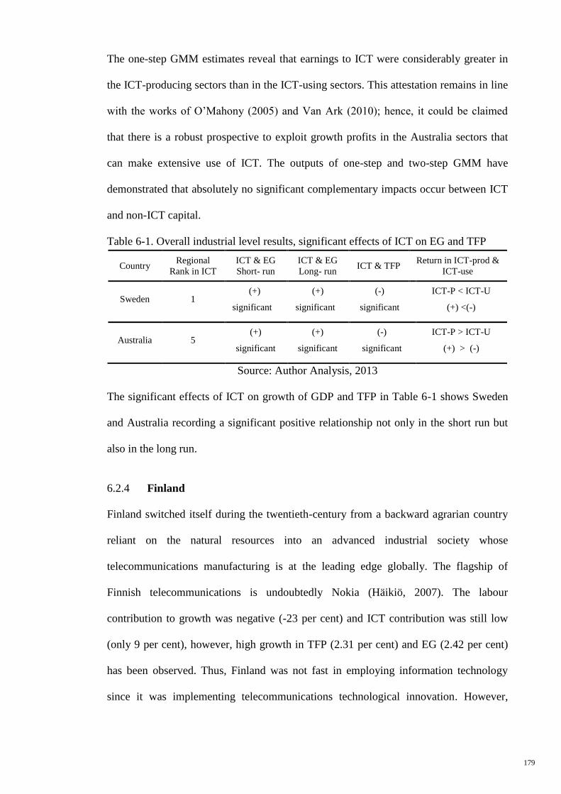
179

The one-step GMM estimates reveal that earnings to ICT were considerably greater in

the ICT-producing sectors than in the ICT-using sectors. This attestation remains in line

with the works of O’Mahony (2005) and Van Ark (2010); hence, it could be claimed

that there is a robust prospective to exploit growth profits in the Australia sectors that

can make extensive use of ICT. The outputs of one-step and two-step GMM have

demonstrated that absolutely no significant complementary impacts occur between ICT

and non-ICT capital.

Table 6-1. Overall industrial level results, significant effects of ICT on EG and TFP

Country Regional

Rank in ICT ICT & EG Short- run

ICT & EG

Long- run ICT & TFP

Return in ICT-prod & ICT-use

Sweden 1 (+)

significant

(+)

significant

(-)

significant

ICT-P < ICT-U

(+) <(-)

Australia 5 (+)

significant

(+)

significant

(-)

significant

ICT-P > ICT-U

(+) > (-)


The significant effects of ICT on growth of GDP and TFP in Table 6-1 shows Sweden

and Australia recording a significant positive relationship not only in the short run but

also in the long run.

6.2.4 Finland

Finland switched itself during the twentieth-century from a backward agrarian country

reliant on the natural resources into an advanced industrial society whose

telecommunications manufacturing is at the leading edge globally. The flagship of

Finnish telecommunications is undoubtedly Nokia (Häikiö, 2007). The labour

contribution to growth was negative (-23 per cent) and ICT contribution was still low

(only 9 per cent), however, high growth in TFP (2.31 per cent) and EG (2.42 per cent)

has been observed. Thus, Finland was not fast in employing information technology

since it was implementing telecommunications technological innovation. However,

180

presently it can be considered as one of the primary producers of information

technology (Ojala, Eloranta, & Jalava, 2006).

We could not find evidence of short run causality running from ICT and non-ICT to

value added growth and TFP, suggesting that GDP and TFP growth have not been

influenced by the contribution of ICT and non-ICT growth. This does not have a

significant impact on these variables in the short run while the long run effects are

significant. This evidence is in a line with Gordon (2000); Jorgenson (2001); Jorgenson

and Stiroh, (2000); Oliner and Siche (2002) who contended that technological progress

in ICT stimulates the growth of total factor productivity in the sectors, and, hence, of

aggregate TFP in the long run.

The results of the causality tests revealed long run bidirectional Granger causality

running from real GDP growth to the contribution of L, ICT, non-ICT, and TFP growth

at the 5% significant level. As a result, contrary to Gholami (2006) and Van Ark et al.

(2003) at the aggregate level, ICT is the determinant factor for economic and TFP

growth in Finland, but only in the long run. There is absolutely no causality relationship

between GDP growth and non-ICT capital in the short run. Specifically, the produced

estimates state that the ICT contribution was 0.37 per cent greater in ICT-producing and

0.33 per cent greater in ICT working with sectors (compared to the remaining sectors).

This evidence is consistent with the findings of Jalava (2003), Jalava and Pohjola (2002,

2007) in that Finland was not as effective in implementing information technology since

it is adapting telecommunications technology. Nokia’s portion of the global mobile

device shop was nearly 35 per cent. This is particularly topical in a country such as

Finland that has enjoyed the advantages of the Nokia phenomenon. For instance, this is

a profitable production of a new technology – however, there is still certainly room for

enhancement in the usage of the new technology in the production procedures of other

181

sectors. Furthermore, no significant complementary issues emerge between ICT and

non-ICT capital.

To sum up, due to the insignificant effects of ICT on growth from the GMM estimators

for Finnish industries, it is not sufficient to just promote industries that produce ICT

equipment and goods. It is equally important that the rest of the economy, as an ICT

consumer, takes on board the ICT-produced industries.

6.2.5 Denmark

Computer software is an essential investment (76 per cent) classification in ICT in

Denmark (Aghion & Howitt, 1997). The ICT contribution is significantly higher than

other factors (38 per cent) where the contribution of TFP to value added is only 9 per

cent in Denmark. Predominantly, the Nordic countries (Denmark, Finland and Sweden)

have related identical high shares for software, which suggests massive diffusion;

however, as yet, this does not seem to have translated into substantial acceleration of the

growth in productivity of these countries (Aghion & Howitt, 1997). In contrast to

Finland, ICT-production industries in Denmark are relatively smaller compared to other

EU countries.

With respect to the ICT impact on output growth, we can perceive that the estimated

short run effect for the period 1990-2007 is insignificant and that the non-ICT, labour

and TFP impacts are also insignificant in the short run. In contrast, all of these

production factors have significant effects on output growth in the long run.

With respect to the causality results for Denmark, this has confirmed the impact of ICT

on total factor productivity as negative (-1.213) and significant at the 5 per cent level.

This evidence is consistent with the productivity paradox that the effects of ICT are

expected with a time lag at the industrial level. However, the major source of TFP

182

growth is annual output growth, which has a significant positive effect on TFP in the

short run (0.886) and long run (0.130).

The results indicated that only long run bidirectional Granger causality is established

among GDP growth and contribution of L, ICT, and non-ICT growth at the 5 per cent

level, respectively. There is a unidirectional long run Granger causality running from

TFP growth to the contribution of ICT, non-ICT, labour and GDP growth at the 5 per

cent significant level whereas short run Granger causality ran from EG to TFP.

Therefore, ICT investment growth cannot be a short run growth policy objective in

Denmark but can be targeted as a long run policy. Danish industries are able to pay

more attention to ICT spillover effects through TFP growth in the short run and

dramatically increase industrial output growth by high TFP in the long run.

System GMM estimates show that the output elasticities of ICT (1.34 per cent) and non-

ICT (1.99 per cent) capital recorded a positive relationship at the 5 per cent significant

level. The general ICT growth contribution is positive and significant in both the one-

step and two-steps results. These results are in line with long run PMG estimators

implying that ICT should be able to play a major role in increasing growth in the Danish

sectors by way of its quicker ICT capital accumulation. Furthermore, ICT was

significantly higher in the ICT-producing industries than ICT-using sectors. This

research is basically in agreement with the works of O’Mahony and Van Ark (2003),

who argued that there is solid potential to exploit growth profits in the EU service

sectors that make extensive use of ICT. However, no significant complementary effects

exist between ICT and non-ICT capital.

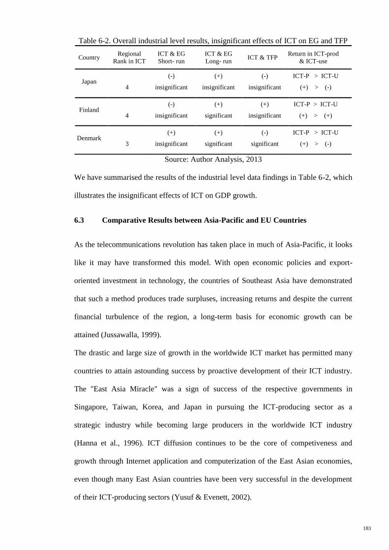
183

Table 6-2. Overall industrial level results, insignificant effects of ICT on EG and TFP

Country Regional

Rank in ICT ICT & EG Short- run

ICT & EG

Long- run ICT & TFP

Return in ICT-prod

& ICT-use

Japan

4

(-)

insignificant

(+)

insignificant

(-)

insignificant

ICT-P > ICT-U

(+) > (-)

Finland

4

(-)

insignificant

(+)

significant

(+)

insignificant

ICT-P > ICT-U

(+) > (+)

Denmark

3

(+)

insignificant

(+)

significant

(-)

significant

ICT-P > ICT-U

(+) > (-)


We have summarised the results of the industrial level data findings in Table 6-2, which

illustrates the insignificant effects of ICT on GDP growth.

6.3 Comparative Results between Asia-Pacific and EU Countries

As the telecommunications revolution has taken place in much of Asia-Pacific, it looks

like it may have transformed this model. With open economic policies and export-

oriented investment in technology, the countries of Southeast Asia have demonstrated

that such a method produces trade surpluses, increasing returns and despite the current

financial turbulence of the region, a long-term basis for economic growth can be

attained (Jussawalla, 1999).

The drastic and large size of growth in the worldwide ICT market has permitted many

countries to attain astounding success by proactive development of their ICT industry.

The "East Asia Miracle" was a sign of success of the respective governments in

Singapore, Taiwan, Korea, and Japan in pursuing the ICT-producing sector as a

strategic industry while becoming large producers in the worldwide ICT industry

(Hanna et al., 1996). ICT diffusion continues to be the core of competiveness and

growth through Internet application and computerization of the East Asian economies,

even though many East Asian countries have been very successful in the development

of their ICT-producing sectors (Yusuf & Evenett, 2002).

184

Based on our results between Asia-Pacific and the EU aggregate level findings, the

highest contribution of ICT was registered by Australia (0.650 Hanna) with a 3.246

Hanna annual GDP growth in the Asia-Pacific group while the top most contributor of

ICT in the EU zone is Switzerland with (1.435 per cent) and 3.283 per cent annual

growth rate. The annual average TFP and GDP growth for Asia-Pacific were 0.861 per

cent and, 3.843 per cent, respectively, over the period 1990-2011, which were greater

than the EU economies with TFP at 0.559 per cent and 2.538 per cent growth rate.

However, the average contribution of ICT growth for Asia-Pacific was 0.482 per cent

during the period, which is smaller than the average EU economies of 0.844 per cent

growth rate. Therefore, it seems that the higher growth rate of GDP in Asia-Pacific than

for the EU countries might be attributable to the ICT contribution. This explains the

lower average ICT contribution in Asia-Pacific countries, which is similar to Vu (2013),

who indicated that the successful growth of Asia relies heavily on investment,

technology catch-up and openness to trade.

Indeed, there are some differences between the Asia-Pacific and the EU when it comes

to ICT and TFP contributions to GDP growth, which could be brought under the

hypothesis of lagging ICT diffusion. This proof implies that ICT developed is not the

only factor presenting differences in productivity and GDP growth between European

and Asia-Pacific countries but that ICT penetration may also have a major role.

Therefore, from the findings it was apparent that ICT contribution to value added across

two regional groups of countries is not strongly correlated with the level of income and

TFP. Consequently, the impacts of the other effective factors of GDP growth should be

controlled by employing more related factors in the model like education, innovation

and trade. A critical feature of the debate over the existence of ICT spillover is whether

the ICT capital stock can also boost economic growth through positive spillover effects

on TFP, if ICT capital is like knowledge capital. Thus, based on the endogenous growth

185

model, new added variables that are related to the spillover effects of ICT have

increased the significance of the model at the aggregate level.

From the causality study, in the short run, in both regions, there is a unidirectional

relationship causality running from economic growth to ICT contribution. In contrast to

the results of Hwan-Joo et al. (2009) for 29 countries, non-ICT contribution has a causal

relationship with economic growth and plays a key role in increasing growth. ICT

contribution does not have a strong interdependent relationship with economic growth

across Asia-Pacific and EU countries between 1990 and 2011. This result is inconsistent

with recent research, which draws attention to the serious weakness of the EU ICT

sector: the lowest efficiency levels are shown by those ICT activities in which most new

value creation is taking place.

The main reason is that the operation in ICT and related services is not fully exploiting

the advantages offered by their network of contacts. This constitutes a major drawback

that constrains the ability of European countries to capitalize on the innovation and

growth-enhancing effects of these activities throughout the economy (García-Muñiz &

Vicente, 2014).

System GMM employs additional instruments compared to the difference GMM, and it

may well not be suitable to apply the System GMM dataset with a small number of

countries. Therefore, we are going to use first-difference GMM for the aggregate level

part due to the small number of countries (N= 6 T= 11) and System GMM for the

industrial level part with large cross-sectional data (N=21, T=17).

TFP growth shows significant and positive effects on GDP growth for both regions

during the two periods with a difference in magnitude, inasmuch as the positive effects

for the Asia-Pacific countries in the second period is higher than for the first period.

However, for the EU, the growth of TFP in the first period is more effective than GDP

186

growth. Overall, the return on TFP growth in the EU is higher than for the Asia-Pacific

countries.

The ICT growth effect only seems to have risen significantly in magnitude during the

1990s and 2000s for the EU countries. While in the Asia-Pacific countries, both the

magnitude and significant effect on GDP growth of ICT during the 2000s declined. This

can be interpreted as ICT being the engine of growth in the 1990s in the Asia-Pacific

countries, whereas it had the same role for the EU economies in the 2000s. This is

similar to the results of previous studies that mentioned that the multiplier effect of the

ICT sectors on the rest of the economy had declined significantly during the period

2000-2005 compared to 1995-2000 (Rohman, 2013). Rohman (2013) applied different

methods like Input-Output (IO) methodology to investigate the contribution of the ICT

sectors to economic performance in the European economies but obtained similar

results to ours.

According to the Asia-Pacific results, between 1990 and 2000, the ICT effect increased

considerably, representing an incredibly positive and significant correlation with output

growth. This attestation highlights the stylised facts displayed in the literature that the

ICT growth contribution enhanced noticeably after 1995, especially in Asia and the US

economies but not in the EU countries. However, for the EU countries, the relative

importance of ICT rose significantly during the second period, from -0.94 to 1.22,

whereas for Asia-Pacific it dropped from 5.214 to -5.915.

These final results confirm that ICT can begin to play a major role in reinforcing growth

among the EU countries, via its faster capital accumulation. Generally, it appears that

when evaluating the results of a couple of group countries, the ICT effect is higher in

the EU economy than for the Asia-Pacific countries not only from the direct effects of

ICT as a capital but also through TFP growth and additional variables by the positive

spillover effect.

187

In the prior investigations on a country with a small ICT-producing sector or without,

should not experience the growth impulses of using ICT capital input. Currently, doubt

concerning the role of the ICT-producing industry has been voiced, specifically from

the viewpoint of reviewing certain EU economies with Asia-Pacific countries. The

current research reveals that for the period under review, the shortage of a large ICT-

producing sector is neither a necessary nor a sufficient condition for countries to enjoy

the growth impacts of ICT. This is exhibited in the case of Australia. While having a

minimal ICT-producing industry, it has clearly reaped the benefit from ICT capital

services.

Generally, there is no discernible systematic relationship between the size of the ICT-

producing industry and the ICT contribution to output growth. This certainly does not

signify that ICT-producing sectors have not contributed to current growth patterns. This

appears from the analyses of the sectoral causes of macro-economic TFP growth

(Colecchia & Schreyer, 2002). For Sweden and Finland, a major section of the overall

TFP growth may be traced back to the ICT-producing sectors (computers,

semiconductors, and communications equipment). Technological improvements also

represent lower equipment prices as well as capital deepening in other sectors; however,

this impact is not linked to the presence of an ICT-producing industry.

From the results reported for five countries, the returns to ICT were higher in ICT-

producing than ICT-using industries, while it seems that ICT-using industries only have

a significantly negative effect on growth in Japanese and Swedish industries. We

conclude that the useful impact of ICT is mainly centred on the ICT intensive sectors.

When the number of ICT-using industries is going to be large in each country, the

significance of ICT capital on value added would also be large, as shown by the results

from Australia and Sweden. These findings are also confirmed by the panel data

analysis of Vu (2011) on a multi-country dataset concerning ICT penetration. Similar to

188

our study, he found a robust result with a causal link between ICT and growth by

employing GMM estimators.

Regardless of the truth that the growth importance of ICT decreased inappreciably

through the second sub-period in Asia-Pacific countries, basically, it is not often used in

ICT growth potential compared to the EU. Consequently, there may be a need for the

Asia-Pacific to provide an environment that is more effective to technology diffusion.

Essentially, the presence of highly skilled labour is of fundamental importance to

maximise the profits from ICT. Despite the fact that the new experience of the EU

economic growth is disappointing compared to the Asia-Pacific countries, the ICT

effect in the Asia-Pacific region was stronger than for the EU.

To sum up the industrial level analysis, according to our results, Sweden’s industries, as

the globally second ranked ICT development indexed country, benefited from ICT-

using more than ICT-producing. Therefore, Swedish industries captured a significant

and positive contribution of ICT either on value added growth or total factor

productivity growth. This is similar to the recent study by Hall, Lotti, & Mairesse

(2013) who mentioned that ICT investment is more important for productivity than

other factors in the EU industries. They also explored the possible complementarity

between R&D and ICT in innovation and production. However, concerning the growth

of Japanese industries, the ICT contribution has not only been considered as an effective

factor on value added and TFP growth but it has a negative impact on TFP growth. This

is associated with the insignificant effects of ICT-using industries in which Japan is

ranked 13th

globally according to the ICT development index.

Even with the requisite institutional and human capital capabilities, it is not sufficient to

just promote industries that produce ICT equipment and goods. It is equally important

that the rest of the economy, as an ICT consumer, takes on board the ICT-produced.

These results have implications for the discourse on economic development in general.

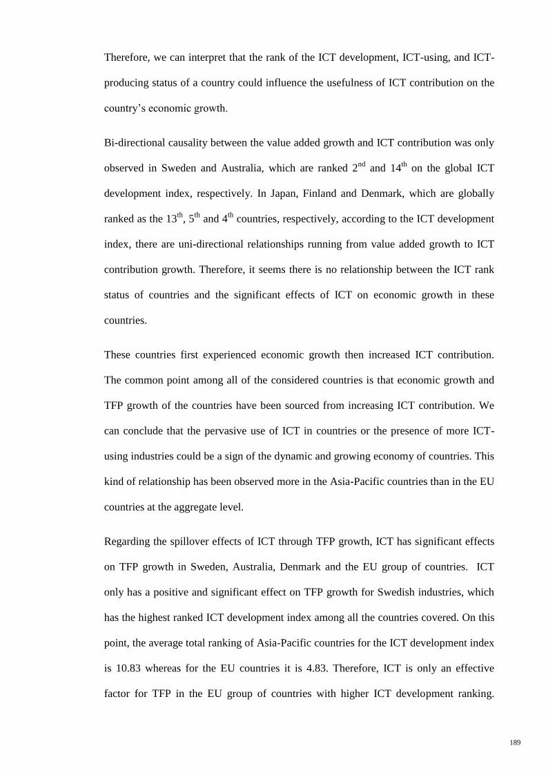
189

Therefore, we can interpret that the rank of the ICT development, ICT-using, and ICT-

producing status of a country could influence the usefulness of ICT contribution on the

country’s economic growth.

Bi-directional causality between the value added growth and ICT contribution was only

observed in Sweden and Australia, which are ranked 2nd

and 14th

on the global ICT

development index, respectively. In Japan, Finland and Denmark, which are globally

ranked as the 13th

, 5th

and 4th

countries, respectively, according to the ICT development

index, there are uni-directional relationships running from value added growth to ICT

contribution growth. Therefore, it seems there is no relationship between the ICT rank

status of countries and the significant effects of ICT on economic growth in these

countries.

These countries first experienced economic growth then increased ICT contribution.

The common point among all of the considered countries is that economic growth and

TFP growth of the countries have been sourced from increasing ICT contribution. We

can conclude that the pervasive use of ICT in countries or the presence of more ICT-

using industries could be a sign of the dynamic and growing economy of countries. This

kind of relationship has been observed more in the Asia-Pacific countries than in the EU

countries at the aggregate level.

Regarding the spillover effects of ICT through TFP growth, ICT has significant effects

on TFP growth in Sweden, Australia, Denmark and the EU group of countries. ICT

only has a positive and significant effect on TFP growth for Swedish industries, which

has the highest ranked ICT development index among all the countries covered. On this

point, the average total ranking of Asia-Pacific countries for the ICT development index

is 10.83 whereas for the EU countries it is 4.83. Therefore, ICT is only an effective

factor for TFP in the EU group of countries with higher ICT development ranking.

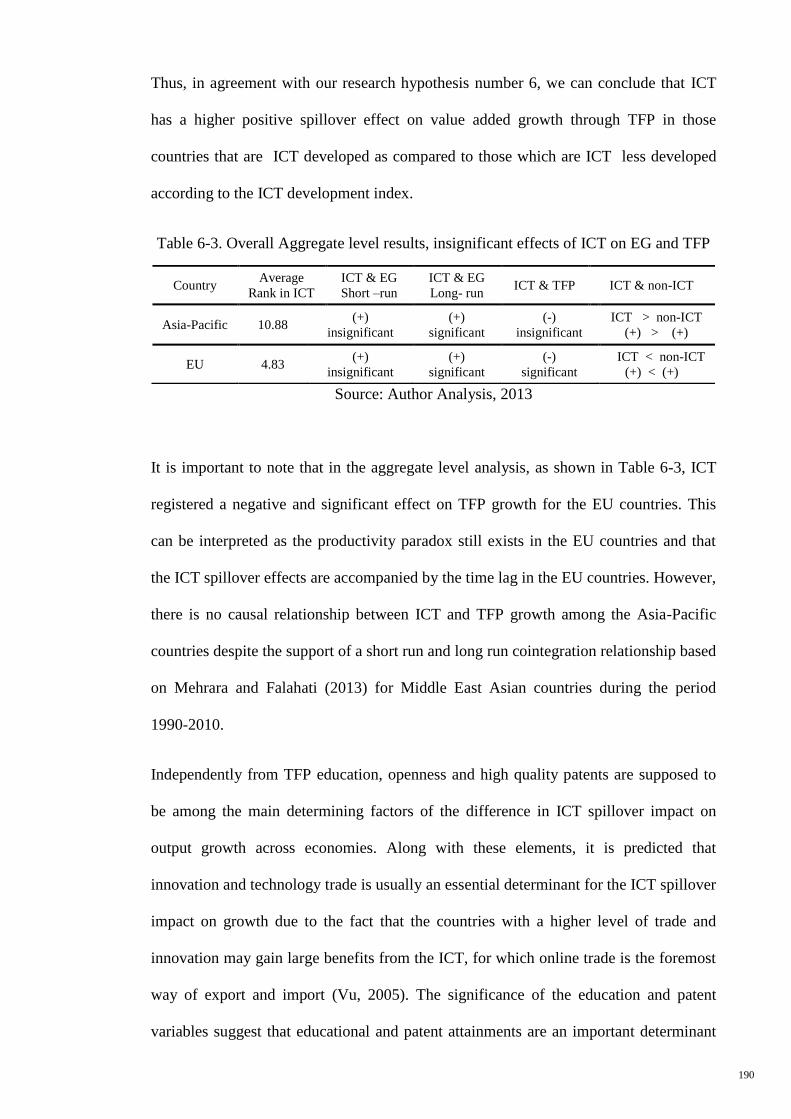
190

Thus, in agreement with our research hypothesis number 6, we can conclude that ICT

has a higher positive spillover effect on value added growth through TFP in those

countries that are ICT developed as compared to those which are ICT less developed

according to the ICT development index.

Table 6-3. Overall Aggregate level results, insignificant effects of ICT on EG and TFP


It is important to note that in the aggregate level analysis, as shown in Table 6-3, ICT

registered a negative and significant effect on TFP growth for the EU countries. This

can be interpreted as the productivity paradox still exists in the EU countries and that

the ICT spillover effects are accompanied by the time lag in the EU countries. However,

there is no causal relationship between ICT and TFP growth among the Asia-Pacific

countries despite the support of a short run and long run cointegration relationship based

on Mehrara and Falahati (2013) for Middle East Asian countries during the period

1990-2010.

Independently from TFP education, openness and high quality patents are supposed to

be among the main determining factors of the difference in ICT spillover impact on

output growth across economies. Along with these elements, it is predicted that

innovation and technology trade is usually an essential determinant for the ICT spillover

impact on growth due to the fact that the countries with a higher level of trade and

innovation may gain large benefits from the ICT, for which online trade is the foremost

way of export and import (Vu, 2005). The significance of the education and patent

variables suggest that educational and patent attainments are an important determinant

Country Average

Rank in ICT ICT & EG Short –run

ICT & EG

Long- run ICT & TFP ICT & non-ICT

Asia-Pacific 10.88 (+)

insignificant (+)

significant (-)

insignificant ICT > non-ICT

(+) > (+)

EU 4.83 (+)

insignificant (+)

significant (-)

significant ICT < non-ICT

(+) < (+)

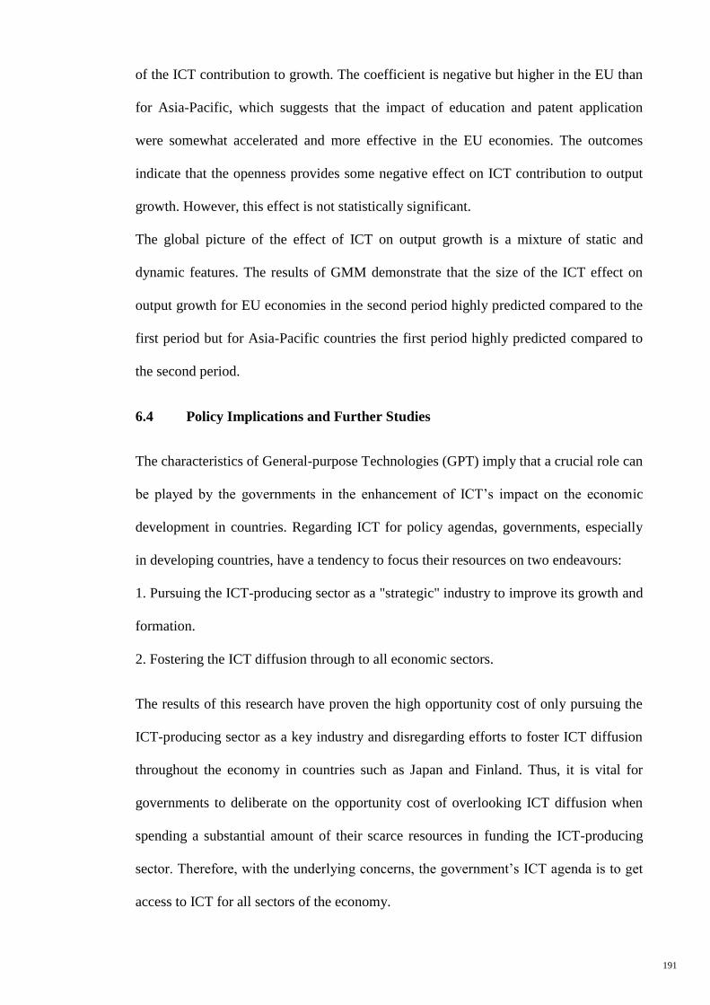
191

of the ICT contribution to growth. The coefficient is negative but higher in the EU than

for Asia-Pacific, which suggests that the impact of education and patent application

were somewhat accelerated and more effective in the EU economies. The outcomes

indicate that the openness provides some negative effect on ICT contribution to output

growth. However, this effect is not statistically significant.

The global picture of the effect of ICT on output growth is a mixture of static and

dynamic features. The results of GMM demonstrate that the size of the ICT effect on

output growth for EU economies in the second period highly predicted compared to the

first period but for Asia-Pacific countries the first period highly predicted compared to

the second period.

6.4 Policy Implications and Further Studies

The characteristics of General-purpose Technologies (GPT) imply that a crucial role can

be played by the governments in the enhancement of ICT’s impact on the economic

development in countries. Regarding ICT for policy agendas, governments, especially

in developing countries, have a tendency to focus their resources on two endeavours:

1. Pursuing the ICT-producing sector as a "strategic" industry to improve its growth and

formation.

2. Fostering the ICT diffusion through to all economic sectors.

The results of this research have proven the high opportunity cost of only pursuing the

ICT-producing sector as a key industry and disregarding efforts to foster ICT diffusion

throughout the economy in countries such as Japan and Finland. Thus, it is vital for

governments to deliberate on the opportunity cost of overlooking ICT diffusion when

spending a substantial amount of their scarce resources in funding the ICT-producing

sector. Therefore, with the underlying concerns, the government’s ICT agenda is to get

access to ICT for all sectors of the economy.

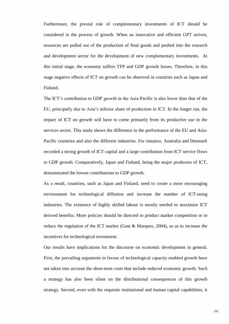
192

Furthermore, the pivotal role of complementary investments of ICT should be

considered in the process of growth. When an innovative and efficient GPT arrives,

resources are pulled out of the production of final goods and pushed into the research

and development sector for the development of new complementary investments. At

this initial stage, the economy suffers TFP and GDP growth losses. Therefore, in this

stage negative effects of ICT on growth can be observed in countries such as Japan and

Finland.

The ICT’s contribution to GDP growth in the Asia-Pacific is also lower than that of the

EU, principally due to Asia’s inferior share of production in ICT. In the longer run, the

impact of ICT on growth will have to come primarily from its productive use in the

services sector. This study shows the difference in the performance of the EU and Asia-

Pacific countries and also the different industries. For instance, Australia and Denmark

recorded a strong growth of ICT capital and a large contribution from ICT service flows

to GDP growth. Comparatively, Japan and Finland, being the major producers of ICT,

demonstrated the lowest contributions to GDP growth.

As a result, countries, such as Japan and Finland, need to create a more encouraging

environment for technological diffusion and increase the number of ICT-using

industries. The existence of highly skilled labour is mostly needed to maximize ICT

derived benefits. More policies should be directed to product market competition or to

reduce the regulation of the ICT market (Gust & Marquez, 2004), so as to increase the

incentives for technological investment.

Our results have implications for the discourse on economic development in general.

First, the prevailing arguments in favour of technological capacity enabled growth have

not taken into account the short-term costs that include reduced economic growth. Such

a strategy has also been silent on the distributional consequences of this growth

strategy. Second, even with the requisite institutional and human capital capabilities, it

193

is not sufficient to just promote industries that produce ICT equipment and goods. This

is due to ICT capital deepening and TFP growth from ICT-goods production,

investment in ICT capital may also enhance TFP growth. This occurs while ICT use

causes spillover impacts and encourages disembodied technical progress. It is equally

important that the rest of the economy, as an ICT consumer, takes on board the ICT-

produced. In both these areas, the state has an important role to play.

Third, digitally stored information (R&D, financing, insurance services, accounting,

payroll, etc.) can already be generated away from the office. The intelligent use of

information is a source of increased productivity, just as natural resources were in the

twentieth-century. The difference is that natural resources are tied to a certain place,

whereas information has no such restrictions. Geography is no longer of the essence, as

everyone has equal access to global information networks. The new restructuring of the

economy may be as great as the one witnessed over 100 years ago when electricity and

the telephone were invented.

Based on the above analyses, it is recommended that a structure for formulating an

efficient government ICT schedule should be in place to foster ICT utilisation and

diffusion across the economy.

The framework contains four main factors – Concepts, Competency, Costs and Benefits

– for both Asian and European countries. A powerful government ICT agenda has to

smartly enhance each of the four components and the interplay among them.

6.4.1 For Asian countries, the suggestions for policy implications

Asian people are less familiar than EU people with the concept and competency of ICT;

therefore, the following may be recommended for Asian countries:

194

1) Concepts

The "Concepts" component concerns the fundamental knowledge of how a country can

gain benefits of ICT revolution in terms of economic growth and development.

Therefore, future research proposals could follow the following components:

Impact of ICT on economic growth and development, and the potential

applications of ICT should be understood profoundly by the policymakers. Furthermore,

they should be mindful of the risks involved due to the lack of strategic planning in

providing the ICT sector with a substantial amount from its limited resources.

Key determinants of ICT diffusion should be comprehended by the

policymakers, which include the educational level, institutional quality and the

openness of the economy of the population. Effective measures for promoting these

determinants assure a fundamental enhancement in the country's capability to reap the

benefits of the ICT spillover effects. Policymakers should be very cautious when

considering market-distorting policies in their ambition to promote ICT diffusion. Once

policymakers have adopted the right concepts, the government ICT agenda has a solid

foundation for a successful implementation.

2) Competency

Human capital or the competency of a population, particularly the labour factor, is the

vital element in a nation's capacity to absorb the penetration of ICT. Thus, we suggest

the following in promoting the "competency" component to enhance the fast diffusion

of ICT:

Introduction of policies and mechanisms that aid the education sector should be

the main focus of investment from both non-government and government sectors.

Additionally, the government should play a proactive role in reforming the education

sector with major investments to make it a key engine driving the economy towards a

knowledge-based economy. Moreover, English fluency should be promoted for Asian

195

countries by the government in applying and endorsing the use of the language in a

variety of training and educational programmes.

Generous and extensive support for ICT-related training should be provided by

encouraging people to augment ICT skills and their understanding of ICT applications.

Moreover, continuous learning should be consistently supported because new

technologies and ICT continue to evolve at a fast pace.

Promoting the quality and commonness of access to ICT services, mainly the

Internet. In particular, governments should be proactive in providing financial

incentives, professional guidance and training for Internet cafes/E-centres, especially in

remote areas.

Encouraging institutional competition increases the depth of ICT diffusion and

controls their development over time.

6.4.2 For European countries, the suggestions for policy implications

With a large consensus that growth in the Asia-Pacific countries has benefited not only

from the production of ICT but also from its adoption of ICT-using industries faster

than the EU, more evidence becomes available that EU countries have taken longer time

to enhance the ICT-using industries. Most European economies show considerably

lower investment levels in ICT goods and software than the Asian countries.

Furthermore, as productivity growth in the Asian countries has accelerated, European

productivity growth has slowed down since the mid-1990s. Therefore, it has been

suggested that EU countries should give more consideration to the cost and benefit

implications of ICT structures in the country:

3) Costs

Cost is a key factor underlying the differences in ICT diffusion. Even for EU countries,

the direct costs of telecommunication services and ICT equipment have also

196

significantly affected their ICT diffusion, as pointed out by Ramirez (2007). The

policies addressing the "Costs" component include the following:

Introducing domestic ICT market and nurturing competition between ICT

equipment vendors.

Relaxing the telecommunication sector through profound and extensive

regulatory reforms intended to lower the costs and improve the service quality.

Encouraging the vibrancy and growth of ICT-related services, which helps

households and firms minimise the cost of investment in ICT.

Presently, telecommunication carriers grant subsidies to encourage the selling of

ICT equipment such as mobile phones; therefore, users are frequently able to purchase

comparatively cheaper units that provide a high degree of functionality. This structure is

certified as having a great impact on the highly functional terminals to broadly enhance

the competitiveness of portable devices in the market. Nonetheless, to provide more

competitively priced products, the debate on substituting the current scheme of funding

with a new price plan should be ongoing.

4) Benefits

While there might be limitations in decreasing the costs of obtaining and using ICT, the

potential for increasing the benefits of investment in ICT is huge. Hence, increasing the

benefit of investment in ICT should be the main emphasis for the government in the

execution due to the increasing contribution of ICT on GDP growth. The benefit of

investment in ICT can be improved in the following ways:

Consistently enhancing the whole business climate by encouraging the openness

of the economy and its assimilation into the worldwide market, nurturing competition

among firms, improving the effectiveness and transparency of the regulatory

framework, and upgrading the quality of governance.

197

Providing incentives and creating solid foundations for the development of e-

commerce.

Making wide-ranging investments on e-government, which permits the citizens

to gain considerable benefits when dealing with the government online.

Encouraging Internet-enabled services, particularly those that deliver

information and consulting services that are critical for firms to improve their global

competitiveness and integration.

Encouraging networking and also collaboration; specifically, establishing

Cluster Initiatives (CIs) that strengthen bonding and cooperation among firms, business

associations with Asian countries. Thus, Asia would be a lucrative market for European

producers. Providing incentives for complementary investments allows firms to reap

higher benefits from investing in ICT. Telecommunication infrastructure significantly

affects both the costs and benefits of investment in ICT, and, therefore, the diffusion of

ICT. For example, Internet applications can be more prolific, and the Internet user can

reap more benefits from the Internet at a lower cost (for less time) if the country is

equipped with a high bandwidth capacity, which determines the quality and speed of

Internet access.

Restructuring the prevailing regulatory framework related to telecommunication

infrastructure development and operation to make it more appropriate for fast changes

prompted by the ICT revolution and globalisation (Vu, 2009).

Advancement of the region's telecommunications industries is going to be

determined by factors, such as the economies of scale versus diseconomies because the

former plays a more determining role in cost reduction than scale economies.

The lesson learnt is that the output and productivity impacts of the new technologies can

be long-delayed. Consequently, current policymakers should consider from whence the

next wave of productivity growth will come. As shown, ICT has already contributed to

198

economic growth by improving productivity in the industries producing ICT equipment.

It has also enhanced capital deepening, i.e. through the substitution of ICT capital for

other forms of capital such as non-ICT. However, the effects on TFP from the re-

organization of production and work are yet to come. The ongoing digitalization and

outsourcing of business processes will result in the restructuring of white-collar work at

the global level, and, consequently, may bring about a new wave of productivity

growth.

In conclusion, although this study has added value to previous works via its wider

coverage sectors in the search for ICT contribution to output and productivity growth in

ICT developed countries of the two regions, there are, however, areas for further

research in ICT contribution. For instance, there is a solid requirement for a better and

longer series of ICT, non-ICT, labour, and TFP contribution data for individual

countries in different industries.

199

REFERENCES

Abramovitz, M. (1989). Thinking about growth: And other essays on economic growth

and welfare: Cambridge University Press.

Aghion, P., & Howitt, P. (1997). Endogenous growth theory: MIT press.

Andrianaivo, M., & Kpodar, K. (2011). ICT, Financial Inclusion, and Growth: Evidence

from African Countries. IMF Working Paper.

Antonelli, C., & Quatraro, F. (2010). The effects of biased technological change on total

factor productivity: empirical evidence from a sample of OECD countries. J

Tchnol Transf, 22(35), 361-383.

Antonopoulos, C., & Sakellaris, P. (2009). The contribution of Information and

Communication Technology investments to Greek economic growth: An

analytical growth accounting framework. Information Economics and Policy,

21(3), 171-191. doi: DOI: 10.1016/j.infoecopol.2008.12.001

Arellano, M., & Bond, S. (1991). Some tests of specification for panel data: Monte

Carlo evidence and an application to employment equations. The Review of

Economic Studies, 58(2), 277-297.

Arellano, M., & Bover, O. (1995). Another look at the instrumental variable estimation

of error-components models. Journal of econometrics, 68(1), 29-51.

Arvanitis, S., & N. Loukis, E. (2009). Information and communication technologies,

human capital, workplace organization and labour productivity: A comparative

study based on firm-level data for Greece and Switzerland. Information

Economics and Policy, 19(21).

Atrostic, B., Boegh-Nielsen, P., Motohashi, K., & Nguyen, S. (2004). IT, Productivity

and Growth in Enterprises: Evidence from new international micro data. The

Economic Impact of ICT–Measurement, Evidence and Implications.

Badescua, M., & Garce´s-Ayerbe, C. n. (2009). The impact of information technologies

on firm productivity :Empirical evidence from Spain. Technovation, 8(29).

Blackburne, E. F., & Frank, M. W. (2009). Estimation of nonstationary heterogeneous

panels. Stata Journal, 7(2), 197-208.

Blomstrom, M., Lipsey, R. E., & Zejan, M. (1996). Is fixed investment the key to

economic growth? : National Bureau of Economic Research.

Bloom, N., Sadun, R., & Van Reenen, J. (2007). Americans do IT better: US

multinationals and the productivity miracle: National Bureau of Economic

Research.

200

Bloom, N., Sadun, R., & Van Reenen, J. (2012). Americans do IT better: US

multinationals and the productivity miracle. The American Economic Review,

102(1), 167-201.

Blundell, R., & Bond, S. (1998). Initial conditions and moment restrictions in dynamic

panel data models. Journal of econometrics, 87(1), 115-143.

Bond, S. R., Hoeffler, A., & Temple, J. (2001). GMM Estimation of Empirical Growth

Models.

Breitung, J. (2000). The local power of some unit root tests for panel data: Humboldt

University of Berlin.

Bresnahan, T. F., & Trajtenberg, M. (1995). General purpose technologies ‘Engines of

growth’? Journal of econometrics, 65(1), 83-108.

Brynjolfsson, E., & Hitt, L. M. (2000). Beyond computation: Information technology,

organizational transformation and business performance. The Journal of

Economic Perspectives, 23-48.

Brynjolfsson, E., & Saunders, A. (2009). Wired for innovation: how information

technology is reshaping the economy: MIT Press.

Chakraborty, C., & Nandi, B. (2003). Privatization, telecommunications and growth in

selected Asian countries: An econometric analysis. Communications and

Strategies, 52(4), 31-47.

Cieślik, A., & Kaniewska, M. (2004). Telecommunications infrastructure and regional

economic development: the case of Poland. Regional Studies, 38(6), 713-725.

Coe, D. T., & Helpman, E. (1995). International r&d spillovers. European Economic

Review, 39(5), 859-887.

Colecchia, A., & Schreyer, P. (2002). ICT investment and economic growth in the

1990s: Is the United States a unique case? A comparative study of nine OECD

countries. [Proceedings Paper]. Review of Economic Dynamics, 5(2), 408-442.

doi: 10.1006/redy.2002.0170

Cortés, E. A., & Navarro, J. A. (2011). Do ICT Influence Economic Growth and Human

Development in European Union Countries? International Advances in

Economic Research, 17(1), 28-44.

Cronin, F. J., Colleran, E. K., Herbert, P. L., & Lewitzky, S. (1993).

Telecommunications and growth: The contribution of telecommunications

infrastructure investment to aggregate and sectoral productivity.

Telecommunications Policy, 17(9), 677-690.

201

Cronin, F. J., Parker, E. B., Colleran, E. K., & Gold, M. A. (1991). Telecommunications

infrastructure and economic growth: An analysis of causality.


Dahl, C., Kongsted, H., & Sørensen, A. (2011). ICT and productivity growth in the

1990s: panel data evidence on Europe. Empirical Economics, 40(1), 141-164.

doi: 10.1007/s00181-010-0421-4

Danish ICT Industry Innovation for Society. (2011).

Datta, P., & Mbarika, V. W. (2006). A global investigation of granger causality between

information infrastructure investment and service-sector growth. The

Information Society, 22(3), 149-163.

Daveri, F. (2002). The New Economy in Europe, 1992-2001. [Article]. Oxford Review

of Economic Policy, 18(3), 345-362.

David, P. A. (1990). The Dynamo and the Computer: An Historical Perspective on the

Modern Productivity Paradox. The American Economic Review, 80(2), 355-361.

doi: 10.2307/2006600

Dedrick, J., Gurbaxani, V., & Kraemer, K. L. (2003). Information technology and

economic performance: A critical review of the empirical evidence. ACM

Computing Surveys, 35(1), 1-28.

Dewan, S., & Kraemer, K. L. (2000). Information technology and productivity:

evidence from country-level data. Management Science, 46(4), 548-562.

Dimelis, S. P., & Papaioannou, S. K. (2011). ICT growth effects at the industry level: A

comparison between the US and the EU. Information Economics and Policy,

23(1), 37-50.

Draca, M., Sadun, R., & Van Reenen, J. (2006). Productivity and ICT: A Review of the

Evidence.

Dutta, A. (2001). Telecommunications and economic activity: An analysis of Granger

causality. Journal of Management Information Systems, 17(4), 71-96.

Eberhardt, M. (2011). Panel time-series modeling: New tools for analyzing xt data.

Paper presented at the United Kingdom Stata Users' Group Meetings 2011.

Eggoh, J. C., Bangake, C., & Rault, C. (2011). Energy consumption and economic

growth revisited in African countries. Energy Policy(0). doi:

10.1016/j.enpol.2011.09.007

Elsadig, A. (2010). Information and Communications Technology Effects on East Asian

Productivity. Journal of the Knowledge Economy, 1(3), 191-201. doi:

10.1007/s13132-010-0013-8

202

Elsadig, M. A. (2008). ICT and Human Capital Intensity Effects on Malaysian

Productivity Growth. International Research Journal of Finance and

Economics, 11(13).

Engelbrecht, H.-J. r., & Xayavong, V. (2006). ICT intensity and New Zealand's

productivity malaise: Is the glass half empty or half full? Information Economics

and Policy (18), 24–42.

Engle, R. F., & Granger, C. W. J. (1987). Co-integration and error correction:

representation, estimation, and testing. Econometrica: journal of the

Econometric Society, 251-276.

Esteban-Pretel, J., Nakajima, R., & Tanaka, R. (2010). TFP growth slowdown and the

Japanese labor market in the 1990s. Journal of the Japanese and International

Economies, 24(1), 50-68. doi: DOI: 10.1016/j.jjie.2009.11.002

Fueki, T., & Kawamoto, T. (2009). Does information technology raise Japan's

productivity? Japan and the World Economy, 21(4), 325-336. doi: DOI:

10.1016/j.japwor.2009.02.001

Fukao, K., Miyagawa, T., Pyo, H. K., & Rhee, K. H. (2009). Estimates of multifactor

productivity, ICT contributions and resource reallocation effects in Japan and

Korea. RIETI Discussion Papear Series.

Gholami, R. (2006). Essays on information and communication technology: Investment,

post-adoption and economic impacts.

Gholami, R., Sang-Yong, T. L., & Heshmati, A. (2006). The Causal Relationship

Between Information and Communication Technology and Foreign Direct

Investment. World Economy, 29(1), 43-62. doi: 10.1111/j.1467-

9701.2006.00757.x

Gholami, R. R., Guo, X. J., Higon, M. D. A., & Lee, S. Y. T. (2009). Information and

Communications Technology (ICT) International Spillovers. [Article]. Ieee

Transactions on Engineering Management, 56(2), 329-340. doi:

10.1109/tem.2009.2016044

Gilchrist, S., Gurbaxani, V., & Town, R. (2001). Productivity and the PC Revolution.

Center for Research on Information Technology and Organizations Working

paper, University of California, disponible en: http://www. crito. uci.

edu/itr/publications/pdf/prod_pc_revolution. pdf, leído el, 12.

Gordon, R. J. (2000). Does the" New Economy" Measure up to the Great Inventions of

the Past? : National Bureau of Economic Research.

203

Granger, C. W. (1981). Some properties of time series data and their use in econometric

model specification. Journal of econometrics, 16(1), 121-130.

Gretton, P., Gali, J., & Parham, D. (2002). Uptake and impacts of ICTs in the Australian

economy: Evidence from aggregate, sectoral.

Gretton, P., Gali, J., & Parham, D. (2004). The effects of ICTs and complementary

innovations on Australian productivity growth. The Economic Impact of ICT:

Measurement, evidence and implications, 105-130.

Groen, J. J. J., & Kleibergen, F. (2003). Likelihood-based cointegration analysis in

panels of vector error-correction models. Journal of Business & Economic

Statistics, 21(2), 295-318.

Grossman, G. M., & Helpman, E. (1991). Trade, knowledge spillovers, and growth.

European Economic Review, 35(2), 517-526.

Gust, C., & Marquez, J. (2004). International comparisons of productivity growth: the

role of information technology and regulatory practices. Labour Economics(11).

Hadri, K. (2000). Testing for stationarity in heterogeneous panel data. The

Econometrics Journal, 3(2), 148-161.

Hadri, K., Guermat, C., & Whittaker, J. (2003). Estimating farm efficiency in the

presence of double heteroscedasticity using panel data. Journal of Applied

Economics, 6(2), 255-268.

Häikiö, L. (2007). Expertise, representation and the common good: grounds for

legitimacy in the urban governance network. Urban Studies, 44(11), 2147-2162.

Hardy, A. P. (1980). The role of the telephone in economic development.


Harper, M., Khandrika, B., Kinoshita, R., & Rosenthal, S. (2010). Nonmanufacturing

industry contributions to multifactor productivity, 1987–2006. Monthly Labor

Review, 16.

Hausman, J. A., & Taylor, W. E. (1981). A generalized specification test. Economics

Letters, 8(3), 239-245.

Hlouskova, J., & Wagner, M. (2006). The performance of panel unit root and

stationarity tests: results from a large scale simulation study. Econometric

reviews, 25(1), 85-116.

Hollanders, H., & Van Cruysen, A. (2008). Rethinking the European Innovation

Scoreboard: A New Methodology for 2008-2010. Inno-Metrics Publication.

Brüssel.

204

Hosseini Nasab, E., & Aghaei, M. (2009). The Effect of ICT on Economic Growth:

Further Evidence. International Bulletin of Business Administration(5).

Howitt, P. (1998). Endogenous Growth Theory. EKO NOMISKA SAM FUNDETS TID

SKRIFT.

Hwan-Joo, S., & Young, S. L. (2006). Contribution of information and communication

technology to total factor productivity and externalities effects. [Article].

Information Technology for Development, 12(2), 159-173. doi:

10.1002/itdj.20021

Hwan-Joo, S., Young, S. L., & Jeong, H. O. (2009). Does ICT investment widen the

growth gap? Telecommunications Policy (33), 10.

Im, K. S., Pesaran, M. H., & Shin, Y. (2003). Testing for unit roots in heterogeneous

panels. Journal of econometrics, 115(1), 53-74.

Inklaar, R., O'Mahony, M., & Timmer, M. (2005). ICT AND EUROPE's

PRODUCTIVITY PERFORMANCE: INDUSTRY‐LEVEL GROWTH

ACCOUNT COMPARISONS WITH THE UNITED STATES. Review of

Income and Wealth, 51(4), 505-536.

Jacobsen, K. F. L. (2003). Telecommunications-a means to economic growth in

developing countries? : Chr. Michelsen Institute.

Jalava, J. (2003). The new economy in Finland: Production and use of ICT. [Article].

Ekonomiska Samfundets Tidskrift, 56(1), 17.

Jalava, J., & Pohjola, M. (2002). Economic growth in the New Economy: evidence from

advanced economies. Information Economics and Policy, 14(2), 189-210. doi:

Doi: 10.1016/s0167-6245(01)00066-x

Jalava, J., & Pohjola, M. (2007). ICT as a source of output and productivity growth in

Finland. Telecommunications Policy, 31(8-9), 463-472. doi: DOI:

10.1016/j.telpol.2007.05.011

Jalava, J., & Pohjola, M. (2008). The roles of electricity and ICT in economic growth:

Case Finland. Explorations in Economic History, 45(3), 270-287. doi: DOI:

10.1016/j.eeh.2007.11.001Japan Economic Update. (2002).

Johansen, S. (1988). Statistical analysis of cointegration vectors. Journal of economic

dynamics and control, 12(2), 231-254.

Johansen, S. (1991). Estimation and hypothesis testing of cointegration vectors in

Gaussian vector autoregressive models. Econometrica: journal of the

Econometric Society, 1551-1580.

205

Jorgenson, D. W. (2001). Information technology and the U.S. economy. AMERICAN

ECONOMIC REVIEW (90(1)), 1-32.

Jorgenson, D. W., Galop, F., & Fraumeni, B. (1987). Productivity and US economic

growth. North-Holland, Amsterdam.

Jorgenson, D. W., Ho, M. S., & Stiroh, K. J. (2003). Growth of US industries and

investments in information technology and higher education. Economic Systems

Research, 15(3), 279-325.

Jorgenson, D. W., & Nomura, K. (2005). The industry origins of Japanese economic

growth. Journal of the Japanese and International Economies, 19(4), 482-542.

doi: DOI: 10.1016/j.jjie.2005.05.002

Jovanovic, B., & Rousseau, P. L. (2005). General purpose technologies. Handbook of

economic growth, 1, 1181-1224.

Jussawalla, M. (1999). The impact of ICT convergence on development in the Asian

region. Telecommunications Policy, 23(3-4), 217-234.

Kao, C., Chiang, M. H., & Chen, B. (1999). International R&D spillovers: an

application of estimation and inference in panel cointegration. Oxford Bulletin of

Economics and statistics, 61(S1), 691-709.

Karner, J., & Onyeji, R. (2007). Telecom private investment and economic growth: The

case of African and Central & East European countries. Jonkoping International

Business School.

Katz, R. (2009). The economic and social impact of telecommunications output.

[Article]. Intereconomics, 44(1), 41-48. doi: 10.1007/s10272-009-0276-0

Kauffman, R. J., & Kumar, A. (2008). Impact of information and communication

technologies on country development: Accounting for area interrelationships.

[Review paper]. International Journal of Electronic Commerce, 13(1), 11-58.

doi: 10.2753/jec1086-4415130101

Kendrick, J. W. (1961). Front matter, Productivity Trends in the United States

Productivity Trends in the United States (pp. -52-50): NBER.

Ketteni, E., Mamuneas, T. P., & Stengos, T. (2007). Nonlinearities in economic growth:

A semiparametric approach applied to information technology data. [Article].

Journal of Macroeconomics, 29(3), 555-568. doi: 10.1016/j.jmacro.2007.03.004

Kiley, M. (1999). Computers and growth with costs of adjustment: will the future look

like the past?

206

Kohli, R., & Devaraj, S. (2003). Measuring information technology payoff: A meta-

analysis of structural variables in firm-level empirical research. Information

Systems Research, 14(2), 127-145.

Kraemer, K. L., & Dedrick, J. (1994). Payoffs from investment in information

technology: Lessons from the Asia-Pacific region. World Development, 22(12),

1921-1931.

Kretschmer, T. (2012). Information and Communication Technologies and Productivity

Growth: A Survey of the Literature: OECD Publishing.

Krugman, P. (1994). The myth of Asia's miracle. Foreign affairs, 62-78.

Lam, P. L., & Shiu, A. (2010). Economic growth, telecommunications development and

productivity growth of the telecommunications sector: Evidence around the

world. Telecommunications Policy, 34(4), 185-199. doi:

10.1016/j.telpol.2009.12.001

Larsson, R., Lyhagen, J., & Löthgren, M. (2008). Likelihood‐based cointegration tests

in heterogeneous panels. The Econometrics Journal, 4(1), 109-142.

Lee, C.-C. (2005). Energy consumption and GDP in developing countries: A

cointegrated panel analysis. Energy Economics, 27(3), 415-427. doi:

10.1016/j.eneco.2005.03.003

Levine, R. (1997). Financial development and economic growth: views and agenda.

Journal of economic literature, 35(2), 688-726.

Li, K. W., & Liu, T. (2011). Economic and productivity growth decomposition: An

application to post-reform China. Economic Modelling, 28(1-2), 366-373. doi:

DOI: 10.1016/j.econmod.2010.08.013

Lind, D. (2008). ICT Production and Productivity in Sweden and Finland, 1975-2004.

International Productivity Monitor, 17, 40-51.

Lindström, T. (2003). The role of high-tech capital formation for Swedish productivity

growth: Konjunkturinstitutet.

Lucas, R. E., Jr. (1988). On the mechanics of economic development. Journal of

Monetary Economics, 22(1), 3-42.

Lucas, R. E., Jr. (1993). Making a Miracle. Econometrica, 61(2), 251-272.

Maddala, G. S., & Wu, S. (1999). A comparative study of unit root tests with panel data

and a new simple test. Oxford Bulletin of Economics and statistics, 61(S1), 631-

652.

Madden, G., & Savage, S. J. (1998). CEE telecommunications investment and

economic growth. Information Economics and Policy, 10(2), 173-195.

207

Madden, G., & Savage, S. J. (2000). R&D spillovers, information technology and

telecommunications, and productivity in ASIA and the OECD. Information

Economics and Policy, 12(4), 367-392.

Maliranta, M., Rouvinen, P., & Airaksinen, A. (2008). IT outsourcing in Finnish

business. Available at SSRN 1141750.

Mamaghani, F. (2010). The Social and Economic Impact of Information and

Communication Technology on Developing Countries: An Analysis. [Article].

International Journal of Management, 27, 607-615.

Mankiw, N. G., Romer, D., & Weil, D. N. (1992). A contribution to the empirics of

economic growth. The quarterly journal of economics, 107(2), 407.

Margaret, W., & Ray, A. (2003). PISA Programme for International Student

Assessment (PISA) PISA 2000 Technical Report: PISA 2000 Technical Report:

oeCd Publishing.

Martínez, D., Rodríguez, J., & Torres, J. (2010). ICT-specific technological change and

productivity growth in the US: 1980–2004. Information Economics and Policy

(22 (2010) ), 121–129.

Mc Morrow, K., Röger, W., & Turrini, A. (2010). Determinants of TFP growth: A close

look at industries driving the EU-US TFP gap. Structural Change and Economic

Dynamics, 21(3),165-180. doi: DOI: 0.1016/j.strueco.2010.03.001.

McCoskey, S., & Kao, C. (1998). A residual-based test of the null of cointegration in

panel data. Econometric reviews, 17(1), 57-84.

Mileva, E. (2007). Using Arellano – Bond Dynamic Panel GMM Estimators in

Stata,Tutorial with Examples using Stata 9.0,(xtabond and xtabond2).

Economics Department,Fordham University.

Mishra, V., Smyth, R., & Sharma, S. (2009). The energy-GDP nexus: Evidence from a

panel of Pacific Island countries. Resource and Energy Economics, 31(3), 210-

220. doi: 10.1016/j.reseneeco.2009.04.002

Miyagawa, T., Ito, Y., & Harada, N. (2004). The IT revolution and productivity growth

in Japan. Journal of the Japanese and International Economies, 18(3), 362-389.

doi: DOI: 10.1016/j.jjie.2004.01.002

Motohashi, K. (2003). Firm level analysis of information network use and productivity

in Japan. Paper presented at the CAED conference, London, September.

Narayan, P. K., Narayan, S., & Popp, S. (2010). Does electricity consumption panel

Granger cause GDP? A new global evidence. Applied Energy, 87(10), 3294-

3298. doi: 10.1016/j.apenergy.2010.03.021

208

Narayan, P. K., & Smyth, R. (2009). Multivariate granger causality between electricity

consumption, exports and GDP: Evidence from a panel of Middle Eastern

countries. Energy Policy, 37(1), 229-236. doi: 10.1016/j.enpol.2008.08.020

Narayana, M. R. (2011). Telecommunications services and economic growth: Evidence

from India. Telecommunications Policy, 35(2), 115-127.

Newey, W. K., & West, K. D. (1987). A simple, positive semi-definite,

heteroskedasticity and autocorrelation consistent covariance matrix.

Econometrica: journal of the Econometric Society, 703-708.

Norton, S. W. (1992). Transaction costs, telecommunications, and the microeconomics

of macroeconomic growth. Economic Development and Cultural Change, 41(1),

175-196.

O'Mahony, M., & Van Ark, B. (2003). EU productivity and competitiveness: an

industry perspective: can Europe resume the catching-up process? : Office for

Official Publications of the European Communities Luxembourg.

O'Mahony, M., & Vecchi, M. (2005). Quantifying the impact of ICT capital on output

growth: a heterogeneous dynamic panel approach. Economica, 72(288), 615-

633.

OECD. (2002). OECD Information Technology Outlook 2002.

OECD. (2003). ICT and Economic Growth: Evidence from OECD Countries, Industries

and Firms: OECD Publishing.

Oh, D., Heshmati, A., & Lööf, H. (2009). Total factor productivity of Korean

manufacturing industries: Comparison of competing models with firm-level

data. Unpublished manuscript.

Ojala, J., Eloranta, J., & Jalava, J. (2006). The road to prosperity: an economic history

of Finland: Suomalaisen Kirjallisuuden Seura.

Oliner, S. D., & Sichel, D. E. (2002). Information technology and productivity: where

are we now and where are we going? : Divisions of Research & Statistics and

Monetary Affairs, Federal Reserve Board.

Pedroni, P. (1999). Critical values for cointegration tests in heterogeneous panels with

multiple regressors. Oxford Bulletin of Economics and statistics, 61(S1), 653-

670.

Pedroni, P. (2004). Panel cointegration: asymptotic and finite sample properties of

pooled time series tests with an application to the PPP hypothesis. Econometric

theory, 597-625.

209

Pesaran, M. H. (2003). On the panel unit root tests using nonlinear instrumental

variables. Available at SSRN 482463.

Pesaran, M. H. (2007). A simple panel unit root test in the presence of cross‐section

dependence. Journal of Applied Econometrics, 22(2), 265-312.

Pesaran, M. H., Shin, Y., & Smith, R. P. (1999). Pooled mean group estimation of

dynamic heterogeneous panels. Journal of the American Statistical Association,

621-634.

Pesaran, M. H., & Smith, R. (1995). Estimating long-run relationships from dynamic

heterogeneous panels. Journal of econometrics, 68(1), 79-113.

Phillips, P. C. B., & Ouliaris, S. (1990). Asymptotic properties of residual based tests

for cointegration. Econometrica: journal of the Econometric Society, 165-193.

Pilat, D. (2004). The ICT productivity paradox: insights from micro data. OECD

Economic Studies. OECD Economic Studies No. 38, 2004/1, 29.

Pohjola, M. (2002). The new economy: facts, impacts and policies. Information

Economics and Policy, 14(2), 133-144.

Quah, D. (2002). Technology Dissemination and Economic Growth: Some Lessons for

the New Economy. Technology and the new economy

Quirós Romero, C., & Rodríguez Rodríguez, D. (2010). E-commerce and efficiency at

the firm level. International Journal of Production Economics, 126(2), 299-305.

doi: DOI: 10.1016/j.ijpe.2010.04.004

Ramirez, M. D. (2007). A panel unit root and panel cointegration test of the

complementarity hypothesis in the Mexican case: 1960–2001. Atlantic

Economic Journal, 35(3), 343-356.

Röller, L. H., & Waverman, L. (2001). Telecommunications infrastructure and

economic development: A simultaneous approach. AMERICAN ECONOMIC

REVIEW, 909-923.

Romer, P. M. (1986). Increasing Returns and Long-Run Growth. Journal of Political

Economy, 94(5), 1002-1037.

Romer, P. M. (1990). Endogenous Technological Change, Journal of Political Economy

98(5, Part 2): The Problem of Development: A Conference of the Institute for

the Study of Free Enterprise Systems, S71-S102.

Roodman, D. (2008). How to do xtabond2: An introduction to difference and system

GMM in Stata.

Schumpeter, J., & Backhaus, U. (2003). The theory of economic development. Joseph

Alois Schumpeter, 61-116.

210

Shao, B. B. M., & Shu, W. S. (2004). Productivity breakdown of the information and

computing technology industries across countries. [Article]. Journal of the

Operational Research Society, 55(1), 23-33. doi: 10.1057/palgrave.jors.2601656

Shepard, S. B. (1997). The new economy: what it really means. Business week, 17, 48-

50.

Shimizu, H., Ogawa, K., & Fujinuma, K. (2006). Information and Communication

Technologies Policy in Japan: Meeting the Challenges Ahead The Global

Information Technology Report (Vol. 2007, pp. 107-116).

Shinjo, K., & Zhang, X. (2004). ICT capital investment and productivity growth:

Granger causality in Japanese and the USA industries. Paper presented at the

15th European Regional International Telecommunications Society Conference

Paper, Retrieved November.

Shiu, A., & Lam, P. L. (2007). Relationships between Economic Growth,

Telecommunications Development and Productivity Growth: Evidence around

the World.

Sichel, D., & Oliner, S. (2002). Information technology and productivity: where are we

now and where are we going? Board of Governors of the Federal Reserve

System FEDS, 29.

Solow, R. M. (1987). We’d better watch out, New York Times Book Review,12 July,p36.

Stiroh, K. J. (2002a). Are ICT spillovers deriving the new economy? Review of Income

and Wealth, 20(series 48), 20.

Stiroh, K. J. (2002b). Information Technology and the US productivity revival: a review

of the evidence; the closer one looks, the more persuasive it is. Business

Economics.

Timmer, M. P., & Van Ark, B. (2005). Does information and communication

technology drive EU-US productivity growth differentials? [Article]. Oxford

Economic Papers-New Series, 57(4), 693-716. doi: 10.1093/oep/gpi032

Toda, H. Y., & Phillips, P. C. B. (1993). Vector autoregressions and causality.

Econometrica: journal of the Econometric Society, 1367-1393.

Triplett, J. E. (1999). The Solow productivity paradox: what do computers do to

productivity? Canadian Journal of Economics Revue canadienne

d’Economique, 32(NO.2).

Triplett, J. E., & Bosworth, B. (2004). Productivity in the US services sector: New

sources of economic growth: Brookings Institution Press.

211

Tseng, C.-Y. (2009). Technological innovation and knowledge network in Asia:

Evidence from comparison of information and communication technologies

among six countries. [Article]. Technological Forecasting and Social Change,

76(5), 654-663. doi: 10.1016/j.techfore.2008.03.007

Turpeinen, O., & Yau, M. K. (1981). Comparisons of results from a three-dimensional

cloud model with statistics of radar echoes on day 261 of GATE. Monthly

Weather Review, 109, 1495-1511.

Uysal, A. H. (2010). IC Development and Economic Growth:An Analysis of

Cointegrating and Causal Relationships with a Panel Data Approach. [Master`s

Thesis in Economics of Innovation and Growth].

Van Ark, B. (2010). Productivity, sources of growth and potential output in the euro

area and the United States. Intereconomics, 1, 17.

Van Ark, B., Inklaar, R., & H. Mc Guckin, R. (2003). ICT and Productivity in Europe

and the United States Where Do the Differences Come From? CESifo Economic

Studies, 49(3), 295–318.

Van Ark, B., & Piatkowski, M. (2004). Productivity, innovation and ICT in Old and

New Europe. International Economics and Economic Policy, 1(2), 215-246. doi:

10.1007/s10368-004-0012-y

Venturini, F. (2009). The long-run impact of ICT. Empirical Economics, 37(3), 497-

515. doi: 10.1007/s00181-008-0243-9

Vourvachaki, E. (2009). Information and Communication Technologies in a Multi-

sector Endogenous Growth Model. Retrieved from

Vu, K. (2005). Measuring the Impact of ICT Investments on Economic Growth.

Submitted to Journal of Economic Growth, October. Retrieved from http://www.

ksg. harvard. edu/cbg/ptep/khuongvu/Papers. htm.

Vu, K. (2009). Embracing the ICT Revolution to Promote Economic Growth in

Developing Countries: Policy Challenges.

Vu, K. (2011). ICT as a source of economic growth in the information age: Empirical

evidence from the 1996-2005 period. Telecommunications Policy, 35(4), 357-

372. doi: DOI: 10.1016/j.telpol.2011.02.008

Weber, D. M., & Kauffman, R. J. (2011). What drives global ICT adoption? Analysis

and research directions. Electronic Commerce Research and Applications, In

Press, Corrected Proof. doi: 10.1016/j.elerap.2011.01.001

212

Welfens, P. J. J. (2008). ICT – productivity and economic growth in Europe. In P. J. J.

Welfens & E. Walther-Klaus (Eds.), Digital Excellence (pp. 13-39): Springer

Berlin Heidelberg.

Westerlund, J., & Edgerton, D. L. (2007). A panel bootstrap cointegration test.

Economics Letters, 97(3), 185-190.

White Paper Information and Communications in Japan. (2012).

Windmeijer, F. (2005). A finite sample correction for the variance of linear efficient

two-step GMM estimators. Journal of econometrics, 126(1), 25-51.

Wolde-Rufael, Y. (2007). Another look at the relationship between telecommunications

investment and economic activity in the United States. International Economic

Journal, 21(2), 199-205.

Wong, P. K. (1998). Leveraging the global information revolution for economic

development: Singapore's evolving information industry strategy. [Article].

Information Systems Research, 9(4), 323-341.

Yoo, S. H. (2006). The causal relationship between electricity consumption and

economic growth in the ASEAN countries. Energy Policy, 34(18), 3573-3582.

doi: 10.1016/j.enpol.2005.07.011

Young, A. (1995). The tyranny of numbers: confronting the statistical realities of the

East Asian growth experience. The quarterly journal of economics, 110(3), 641-

680.

Yusuf, S., & Evenett, S. J. (2002). Can East Asia compete?: innovation for global

markets: World Bank-free PDF.

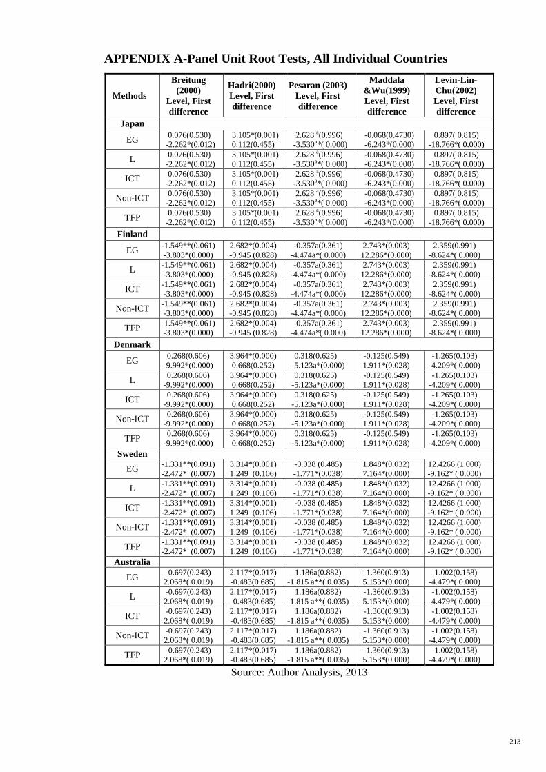
213

APPENDIX A-Panel Unit Root Tests, All Individual Countries

Methods

Breitung

(2000)

Level, First

difference

Hadri(2000)

Level, First

difference

Pesaran (2003)

Level, First

difference

Maddala

&Wu(1999)

Level, First

difference

Levin-Lin-

Chu(2002)

Level, First

difference

Japan

EG 0.076(0.530)

-2.262*(0.012)

3.105*(0.001)

0.112(0.455)

2.628 a(0.996)

-3.530a*( 0.000)

-0.068(0.4730)

-6.243*(0.000)

0.897( 0.815)

-18.766*( 0.000)

L 0.076(0.530)

-2.262*(0.012)

3.105*(0.001)

0.112(0.455)

2.628 a(0.996)

-3.530a*( 0.000)

-0.068(0.4730)

-6.243*(0.000)

0.897( 0.815)

-18.766*( 0.000)

ICT 0.076(0.530)

-2.262*(0.012)

3.105*(0.001)

0.112(0.455)

2.628 a(0.996)

-3.530a*( 0.000)

-0.068(0.4730)

-6.243*(0.000)

0.897( 0.815)

-18.766*( 0.000)

Non-ICT 0.076(0.530)

-2.262*(0.012)

3.105*(0.001)

0.112(0.455)

2.628 a(0.996)

-3.530a*( 0.000)

-0.068(0.4730)

-6.243*(0.000)

0.897( 0.815)

-18.766*( 0.000)

TFP 0.076(0.530)

-2.262*(0.012)

3.105*(0.001)

0.112(0.455)

2.628 a(0.996)

-3.530a*( 0.000)

-0.068(0.4730)

-6.243*(0.000)

0.897( 0.815)

-18.766*( 0.000)

Finland

EG -1.549**(0.061)

-3.803*(0.000)

2.682*(0.004)

-0.945 (0.828)

-0.357a(0.361)

-4.474a*( 0.000)

2.743*(0.003)

12.286*(0.000)

2.359(0.991)

-8.624*( 0.000)

L -1.549**(0.061)

-3.803*(0.000)

2.682*(0.004)

-0.945 (0.828)

-0.357a(0.361)

-4.474a*( 0.000)

2.743*(0.003)

12.286*(0.000)

2.359(0.991)

-8.624*( 0.000)

ICT -1.549**(0.061)

-3.803*(0.000)

2.682*(0.004)

-0.945 (0.828)

-0.357a(0.361)

-4.474a*( 0.000)

2.743*(0.003)

12.286*(0.000)

2.359(0.991)

-8.624*( 0.000)

Non-ICT -1.549**(0.061)

-3.803*(0.000)

2.682*(0.004)

-0.945 (0.828)

-0.357a(0.361)

-4.474a*( 0.000)

2.743*(0.003)

12.286*(0.000)

2.359(0.991)

-8.624*( 0.000)

TFP -1.549**(0.061)

-3.803*(0.000)

2.682*(0.004)

-0.945 (0.828)

-0.357a(0.361)

-4.474a*( 0.000)

2.743*(0.003)

12.286*(0.000)

2.359(0.991)

-8.624*( 0.000)

Denmark

EG 0.268(0.606)

-9.992*(0.000)

3.964*(0.000)

0.668(0.252)

0.318(0.625)

-5.123a*(0.000)

-0.125(0.549)

1.911*(0.028)

-1.265(0.103)

-4.209*( 0.000)

L 0.268(0.606)

-9.992*(0.000)

3.964*(0.000)

0.668(0.252)

0.318(0.625)

-5.123a*(0.000)

-0.125(0.549)

1.911*(0.028)

-1.265(0.103)

-4.209*( 0.000)

ICT 0.268(0.606)

-9.992*(0.000)

3.964*(0.000)

0.668(0.252)

0.318(0.625)

-5.123a*(0.000)

-0.125(0.549)

1.911*(0.028)

-1.265(0.103)

-4.209*( 0.000)

Non-ICT 0.268(0.606)

-9.992*(0.000)

3.964*(0.000)

0.668(0.252)

0.318(0.625)

-5.123a*(0.000)

-0.125(0.549)

1.911*(0.028)

-1.265(0.103)

-4.209*( 0.000)

TFP 0.268(0.606)

-9.992*(0.000)

3.964*(0.000)

0.668(0.252)

0.318(0.625)

-5.123a*(0.000)

-0.125(0.549)

1.911*(0.028)

-1.265(0.103)

-4.209*( 0.000)

Sweden

EG -1.331**(0.091)

-2.472* (0.007)

3.314*(0.001)

1.249 (0.106)

-0.038 (0.485)

-1.771*(0.038)

1.848*(0.032)

7.164*(0.000)

12.4266 (1.000)

-9.162* ( 0.000)

L -1.331**(0.091)

-2.472* (0.007)

3.314*(0.001)

1.249 (0.106)

-0.038 (0.485)

-1.771*(0.038)

1.848*(0.032)

7.164*(0.000)

12.4266 (1.000)

-9.162* ( 0.000)

ICT -1.331**(0.091)

-2.472* (0.007)

3.314*(0.001)

1.249 (0.106)

-0.038 (0.485)

-1.771*(0.038)

1.848*(0.032)

7.164*(0.000)

12.4266 (1.000)

-9.162* ( 0.000)

Non-ICT -1.331**(0.091)

-2.472* (0.007)

3.314*(0.001)

1.249 (0.106)

-0.038 (0.485)

-1.771*(0.038)

1.848*(0.032)

7.164*(0.000)

12.4266 (1.000)

-9.162* ( 0.000)

TFP -1.331**(0.091)

-2.472* (0.007)

3.314*(0.001)

1.249 (0.106)

-0.038 (0.485)

-1.771*(0.038)

1.848*(0.032)

7.164*(0.000)

12.4266 (1.000)

-9.162* ( 0.000)

Australia

EG -0.697(0.243)

2.068*( 0.019)

2.117*(0.017)

-0.483(0.685)

1.186a(0.882)

-1.815 a**( 0.035)

-1.360(0.913)

5.153*(0.000)

-1.002(0.158)

-4.479*( 0.000)

L -0.697(0.243)

2.068*( 0.019)

2.117*(0.017)

-0.483(0.685)

1.186a(0.882)

-1.815 a**( 0.035)

-1.360(0.913)

5.153*(0.000)

-1.002(0.158)

-4.479*( 0.000)

ICT -0.697(0.243)

2.068*( 0.019)

2.117*(0.017)

-0.483(0.685)

1.186a(0.882)

-1.815 a**( 0.035)

-1.360(0.913)

5.153*(0.000)

-1.002(0.158)

-4.479*( 0.000)

Non-ICT -0.697(0.243)

2.068*( 0.019)

2.117*(0.017)

-0.483(0.685)

1.186a(0.882)

-1.815 a**( 0.035)

-1.360(0.913)

5.153*(0.000)

-1.002(0.158)

-4.479*( 0.000)

TFP -0.697(0.243)

2.068*( 0.019)

2.117*(0.017)

-0.483(0.685)

1.186a(0.882)

-1.815 a**( 0.035)

-1.360(0.913)

5.153*(0.000)

-1.002(0.158)

-4.479*( 0.000)


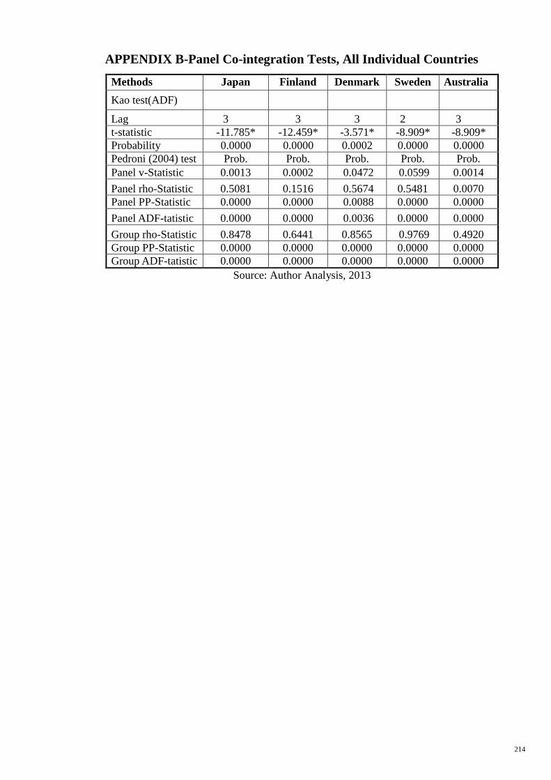
214

APPENDIX B-Panel Co-integration Tests, All Individual Countries

Methods Japan Finland Denmark Sweden Australia

Kao test(ADF) Lag 3 3 3 2 3 t-statistic -11.785* -12.459* -3.571* -8.909* -8.909* Probability 0.0000 0.0000 0.0002 0.0000 0.0000 Pedroni (2004) test Prob. Prob. Prob. Prob. Prob. Panel v-Statistic 0.0013 0.0002 0.0472 0.0599 0.0014 Panel rho-Statistic 0.5081 0.1516 0.5674 0.5481 0.0070 Panel PP-Statistic 0.0000 0.0000 0.0088 0.0000 0.0000 Panel ADF-tatistic 0.0000 0.0000 0.0036 0.0000 0.0000 Group rho-Statistic 0.8478 0.6441 0.8565 0.9769 0.4920 Group PP-Statistic 0.0000 0.0000 0.0000 0.0000 0.0000 Group ADF-tatistic 0.0000 0.0000 0.0000 0.0000 0.0000


Documents

THE CONTRIBUTION OF INFORMATION COMMUNICATION …studentsrepo.um.edu.my/4630/1/Final_Vesrion_of_Ph.D_Thesis.18_March_2014.pdfthe contribution of information communication technology