Embed Size (px)
Citation preview

This is an Open Access document downloaded from ORCA, Cardiff University's institutional
repository: http://orca.cf.ac.uk/64909/
This is the author’s version of a work that was submitted to / accepted for publication.
Citation for final published version:
Abdul Wahab, Nor Shaipah and Holland, Kevin 2015. The persistence of book-tax differences. The
British Accounting Review 47 (4) , pp. 339-350. 10.1016/j.bar.2014.06.002 file
Publishers page: http://dx.doi.org/10.1016/j.bar.2014.06.002
<http://dx.doi.org/10.1016/j.bar.2014.06.002>
Please note:
Changes made as a result of publishing processes such as copy-editing, formatting and page
numbers may not be reflected in this version. For the definitive version of this publication, please
refer to the published source. You are advised to consult the publisher’s version if you wish to cite
this paper.
This version is being made available in accordance with publisher policies. See
http://orca.cf.ac.uk/policies.html for usage policies. Copyright and moral rights for publications
made available in ORCA are retained by the copyright holders.

1
The Persistence of Book-Tax Differences
Nor Shaipah Abdul Wahab and Kevin Holland
February 2014
Affiliations: The authors are respectively; Lecturer in Accounting at School of Management, University of Southampton UK, and Professor of Accounting and Taxation, Cardiff Business School, Cardiff University. Address for correspondence: Dr. Nor Shaipah Abdul Wahab, School of Management, University of Southampton, Highfield, Southampton, SO17 1BJ UK. [email protected] Acknowledgements: The authors are grateful for the helpful comments from seminar and conference participants at School of Management, University of Southampton (2012) and British Accounting and Finance Association, Newcastle (2013) and in particular Rahma Addeh and Sarah Lindop.
2
The Persistence of Book-Tax Differences
Abstract:
Academic researchers and policy activists have used the difference between
accounting income and estimated taxable income, commonly referred to as the
book-tax difference (BTD) as a proxy of the unobservable level of corporate income
tax planning. In drawing any policy implications from observed BTDs, an
understanding of the sources of BTDs and their properties is important. In
particular, identifying the degree of persistence or representativeness of an
observed annual BTD is critical.
To the authors’ knowledge, this paper is the first to examine how BTDs and
their components e.g. permanent differences, temporary differences and the effect
of differences between UK and overseas statutory tax rate behave over time. The
necessary data disclosed under IAS 12 Income Taxes (IASB, 2010) has only been
systematically publicly disclosed in the UK since 2005.
In summary, the results indicate that the degree of persistence is dependent
on the nature of the BTD and that this variation in persistence itself varies by
industry group. The most persistence component relates to differences between UK
and overseas statutory tax rates with temporary differences being the least
persistent, indicative of a non-earnings management motivation. Within industry
groupings there is wide variation in the level of persistence. While 59.4% of the
sample companies experienced only one change of sign BTD at most in the six year
period, the balance of the sample had at least two changes.
3
The Persistence of Book-Tax Differences
1. Introduction
A recent phenomenon is the increased scrutiny of the level of corporate
income tax paid by companies (Whiting, 2006). Companies have often attracted
adverse attention because of a perceived discrepancy between the level of
accounting profits reported and the associated levels of taxable income and
consequentially, the level of corporate income tax payable e.g. UK Uncut (2010) and
Public Accounts Committee (2012). In general terms the scrutiny reflects concerns
over companies’ use of tax avoidance techniques and the perceived consequences
on levels of government revenues and increased levels of taxation on other
taxpayer groups (The Guardian, 2009; Trade Union Congress, 2009; UK Uncut,
2010; New Statesman, 2011 and Christian Aid, 2012). Hasseldine, Holland & Van
der Rijt (2012) show that tax administrations have responded in a number of ways.
These include the publication of UK Tax Gap statistics by HMRC in 2009 for the first
time and the introduction into UK legislation of a General Anti Avoidance Rule –
GAAR (HMRC 2013). Further afield intergovernmental organisations have published
proposals to “combat” tax avoidance e.g. EU (2013) and OECD (2013).
Companies are required to calculate two measures of income on an annual
basis. One measure is determined by financial reporting regulations to give
accounting or book income while the second uses tax law to produce a figure of
taxable income. The degree to which the resulting levels of income correspond
depends on the extent of conformity between the two measures (Hanlon, 2005).
Any difference between the two levels is commonly referred to as the book-tax
difference (BTD). Emphasising the importance of BTDs, “large” US corporations have
been required to file with the Internal Revenue Service (IRS) a reconciliation

4
(Schedule M-3) of taxable income and financial accounting income since 2004
(Boynton & Mills, 2004).
In response to BTDs, there have been calls to require conformity between the
two income measures to end “arbitraging” between the two measures i.e. reporting
accounting income that is not included in taxable income and to increase the
reliability of reported accounting income by removing the greater flexibility
available under financial reporting standards compared with tax legislation (Desai,
2005). However, advocates of the current position argue such conformity would
lead to a loss of information content by removing this flexibility through which
managers can signal private information (Hanlon, Maydew & Shevlin, 2008). These
studies examine the persistence of accounting income i.e. the relation between
accounting earnings in successive periods.
We examine a different question by focusing for the first time on the
persistence of annual BTDs. While BTDs as can arise for a number of reasons
including tax planning, a passive interaction between accounting and tax based
income definitions and earnings management (Graham, Raedy & Shackelford, 2012),
we use IAS 12 Income Taxes (IASB 2010) to examine aggregate and disaggregated
BTDS.1 This allows separate consideration of permanent and temporary differences
in the income measures, and the effect on of income being taxable in overseas
jurisdictions with statutory tax rates that differ from the UK rate. Using
disaggregated measures allows a better understanding of the underlying
motivation. The sample comprises a panel of UK quoted non-financial companies
over the six year period 2005 – 2010 and comprises 798 company-year
observations.
The paper contributes to the literature on corporate tax performance by
analysing the dynamic processes which give rise to BTDs in three aspects. Firstly,
whether the sign of BTDs i.e. whether accounting income is higher or lower than
5
estimated taxable income, changes over time or is consistent, affects the validity of
using a single (annual) observation as a representative measure of corporate income
tax behaviour and the conclusions that can be drawn. This has direct implications
when analysing corporate performance in terms of after tax income performance
and more widely in terms of judging corporate behaviour with respect to broader
societal expectations. Secondly, it provides an insight into corporate behaviour. A
positive (negative) serial correlation in BTDs infers companies consistently
(temporarily) maintaining the relative levels of accounting and taxable income.
Thirdly, to the extent these dynamics vary by company is an indicator of company
specific tax behaviour and provides a measure of the extent to which companies
deviate from their peers. This can have implications for the effectiveness of
regulatory policy with respect to both taxation and accounting.
In summary, the results indicate that the degree of persistence is dependent
on the nature of the BTD and that this variation in persistence itself varies by
industry group. The most persistence component relates to differences between UK
and overseas statutory tax rates with temporary differences being the least
persistent indicative of a non-earnings management motivation. Within industry
groupings there is wide variation in the level of persistence. While 59.4% of the
sample companies experienced only one change of sign BTD at most in the six year
period, the balance had at least two changes.
This paper proceeds as follows: Section 2 presents a review of relevant
literature and is followed by Section 3 on sample and data, Section 4 explains the
research design while Section 5 presents the results of the analysis and Section 6
contains a discussion and the paper’s conclusions.
2. Literature review
6
The concept of persistence is familiar in research examining the quality of
accounting earnings where higher (lower) temporal correlation in accounting
earnings is interpreted as indicative of higher (lower) quality of earnings (Sloan
1996). This approach has also been used to examine the relative information
content of accounting earnings and cash flow by decomposing accounting earnings
into cashflows from operations and accounting accruals. Sloan (1996) found a
higher persistence between cashflows and next period accounting earnings than
with accounting accruals and next period accounting earnings. This lower quality in
accounting accruals is attributed to the flexibility and subjectivity involved in their
calculation which allows a greater independence between successive values.
Hanlon (2005) and Blaylock, Shevlin & Wilson (2012) examined the
information content of BTDs by the extent to which they moderate the relation
between current period accruals and next period accounting earnings. BTDs as a
summary measure of the comparison between two income measurement systems
can provide additional information on earnings persistence beyond that in the
accounting earnings figure (Hanlon, 2005). Taxable income may be a more robust
measure less liable to management and therefore BTDs may be indicative of the
extent of earnings management (Desai, 2005, Abdul Wahab &,Holland, 2012).
Hanlon (2005) finds that the relation between accounting accruals and next period
accounting earnings is moderated by the level of BTDs with higher BTDs being
associated with lower earnings persistence. Raedy, Seidman and Shackelford (2011)
use disaggregated BTDs to extend Hanlon (2005) and conclude that investors price
all components of the BTD equally irrespective of their differing nature; a result they
described as “baffling” given the differing cashflows effects of the various sources
of BTDs.
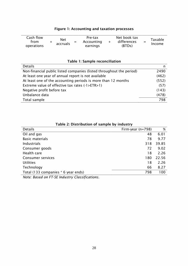
XXX Insert figure 1 about here XXX
7
In viewing this paper it is useful to consider the processes involved in
generating accounting earnings and taxable income measures, this is shown in
figure 1. The earnings persistence literature reviewed above concentrates on the
information content of current accounting earnings or decomposed accounting
earnings in forecasting future accounting earnings. Instead we focus on the
persistency of BTDs in their own right.
Although there is limited research on BTDs we are not aware of any which
examines their persistence. While Plesko & Weber (2009) examine the time series
properties of accounting income and taxable income they do not examine BTDs.
Their focus is on the use of accounting data to forecast taxable income in order to
estimate marginal corporate income tax rates. Their finding that book and taxable
income have similar persistence coefficients is conducive to using accounting
income in forecasting future taxable income. Dyreng, Hanlon & Maydew (2008)
examine long term tax avoidance and find a weak relation between annual and long
term (five and ten years) cash Effective Tax Rates (ETRs) and highlight the
significant year to year variation in annual ETRS.2,3 This variability is reflected in the
majority of companies (>73%) not being able to maintain a consistently low ETR at
below 20% compared to a mean rate of 30%. Although Chen, Dhaliwal & Trombley
(2012) use the concept of consistency in connection with BTDs to extend Hanlon
(2005), their focus is on its moderating effect on the relation between accruals and
future accounting earnings rather the properties of consistency.
From a tax planning perspective, BTDs can be decomposed into permanent
differences (PDs) and temporary differences (TDs) between accounting and taxable
income definitions (Dyreng et al., 2008; Donohoe & McGill, 2011; Tang & Firth,
2011). PDs arise in a single year because of differences between the two income
8
measures in how a transaction is treated (Wilson, 2009). The level of PDs can reflect
strategic tax management (Frank, Lynch & Rego, 2009).
The second source of tax planning related BTDs arises because of temporal
differences between accounting and taxable income measures resulting in a
transaction being included in both accounting and taxable income measures though
not simultaneously e.g. relief for qualifying expenditure on plant and machinery,
and utilisation of loses (Altshuler, Auerbach, Cooper & Knittel, 2009; Shackelford,
Slemrod & Sallee, 2011). Although the ultimate effect of TDs on a period’s
accounting reported tax expense is almost absent, they affect the tax expense
composition (Maydew & Shackelford, 2007) and have a cash flow timing affect.
While TDs can represent tax avoidance in the form of tax deferral, Frank et al.
(2009) caution that TDs can also arise from non-discretionary differences e.g.
differences between non tax deductible accounting deprecation and tax deductible
capital allowances. There is second dimension to the persistence of TDs. Although
by definition TDs only produce a temporary BTD, if a company can generate net new
TDs consistently over time through continual tax planning the effect is more
permanent.
BTDs can also arise from earnings management. This is more likely to
represent PDs which can imply managerial aggressiveness in financial accounting
reporting (Hanlon & Slemrod, 2009). However, companies may be willing to pay
corporate income tax on managed earnings as a signal of their credibility (Erickson,
Hanlon & Maydew, 2004) and therefore include the managed earnings in both
accounting and taxable income measures. Earnings management in the form of
accelerating income recognition or deferring expense recognition would not change
the composition of the overall tax change even in the unlikely event of a company
adjusting (reversing) the effects of accounting earnings management when
estimating corporate income tax liability.4

9
A third aspect of tax planning can be identified in the context of IAS 12
Income Tax mandated disclosures and BTDs. Taxable income subject to a statutory
tax rate (STR) which differs from the rate prevailing in a company’s home
jurisdiction will give rise to a higher or lower current tax expense than would be the
case if the income was only taxable at the domestic STR (Bucovetsky & Haufler,
2008; Devereux, Lockwood & Redoano, 2008). We use the term Statutory Tax Rate
Difference (STRD) to describe the net overall effect of differences in statutory tax
rates and tax base definitions between the UK and other tax jurisdictions in which a
firm operates. This measure can provide forward-looking information to
shareholders in assessing the consistency of companies’ tax management activities
(Schmidt, 2006). We also include STRD in our examination of the persistence of
BTDs, PDs and TDs.
The ability to generate BTDs or the circumstances that generate them may
be firm specific e.g. senior managements’ preferences (Dyreng, Hanlon and
Maydew, 2010), or industry specific level. The influence of distinctive industry
effects on companies’ tax charges has been long researched, for example,
Harberger (1959) and Grieson, Hamovitch, Levenson & Morgenstern (1977).
Industry membership can be relevant because of industry specific tax treatments in
credit, incentives and allowance (Omer, Molloy & Ziebart, 1993; Holland, 1998; Kim
& Limpaphayom, 1998; McIntyre & Nguyen, 2000). Further differences in industry
conditions, for example, risk, competitiveness and asset structure, can explain
variations in companies’ capital and operating expenditure with consequential
variations tax liability (Bradley, Jarrell & Kim, 1984; Kovenock & Phillips, 1997).
In summary, BTDs and their components PDs, TDs and STRDs have potential
information content to interested parties. An understanding of the stability and
persistency of these items can help shareholders, tax administrations and society
more generally, understand the processes underlying companies’ tax performance.
10
3. Sample and data
This paper analyses financial reporting disclosed tax data of a sample of
companies listed on the London Stock Exchange for the six year period 2005 to
2010. The sample is restricted to non-financial companies to reduce complexities
from variations in financial reporting regulations. Further, companies with extreme
effective tax rates (ETRs), i.e. ETRs value outside the range ± 1 were excluded to
control for the potential bias of nonrecurring statutory reconciliation items.5 Such
items could be due to effects of unusual activity, for example, business dispositions
and asset impairments (Phillips, 2003). Table 1 presents the summary of the sample
reconciliation.
XXX Insert Table 1 about here XXX
As the effective tax rate reconciliation notes in the companies’ financial
statements are not in machine readable form, the required tax data was hand
gathered from the tax footnotes of each firm. IAS 12 Income Tax requires the
disclosure of a company’s total corporate income Tax Expense (TE), separately
identifying the current tax expense (CTE) and deferred tax expense (DTE). Further,
a reconciliation between TE and the notional tax charge, i.e. the corporate income
tax liability that would be expected by applying the current (UK) statutory tax rate
to the current accounting profit is required.6 Specifically the reconciliation
summaries the effect of, permanent differences (PD) between accounting and
taxable income measures, differences between UK and foreign statutory tax rates
(STRD) and disclosures the UK Statutory Tax Rate applying during the period.7
Further, disclosure of (i) “the amount of deferred tax expense (income) relating to
changes in tax rates or the imposition of new taxes”; and (ii) “the amount of the
benefit arising from a previously unrecognised tax loss, tax credit or temporary
11
difference of a prior period that is used to reduce current tax expense [or deferred
tax expense]” (IAS 12 para 80, IASB, 2010) enables the effects of such amounts,
along with any prior year adjustments, to be removed from the TE to ensure it is
free of distorting effects relating to other periods.8 In turn the separate disclosure
of DTE allows the effect of temporary differences (TD) between accounting and
taxable income measures to be quantified.
Table 2 presents the distribution of the companies across industry
classification (n=798). In the sample, there are more companies in the industrial
sector (39.85%), than in consumer services (22.56%) and basic materials (9.77%).
The relative distribution of the remaining industries is as follows: consumer goods,
technology, oil and gas, health care and utilities.
XXX Insert Table 2 about here XXX
4. Research design
Identification of BTD and components
We use companies’ annual accrued corporate income tax charges to estimate
BTDs. This involves taking the disclosed pre-tax accounting earnings and
estimating taxable income. Hanlon (2003) and Donohoe, McGill and Outslay (2012)
summarise limitations in using US accounting date to estimate taxable income.
Three major potential sources of error exist: (1) transactions that do not generate
permanent or temporary book-tax differences, (2) research and development tax
credits, and (3) tax rate differentials between domestic and foreign operations. The
first condition holds in a UK/IFRS setting in that conforming differences i.e. items
that do not appear in either accounting or taxable income, will escape
measurement. However, the incentive for companies to enter into permanent
confirming differences is likely to be low for quoted companies facing market
expectations for increased reported accounting income (Erickson et al. 2004,
12
Hanlon & Heitzman, 2010). The information in the IAS 12 tax reconciliation allows
the second limitation to be overcome and the third reduced as discussed below.
However, the overall conclusion remains that as in all jurisdictions where public
access to companies’ tax returns is not routinely available, estimates of taxable
income using only publically available information will measure underlying taxable
income with error. However, in this setting the source of the error can be identified.
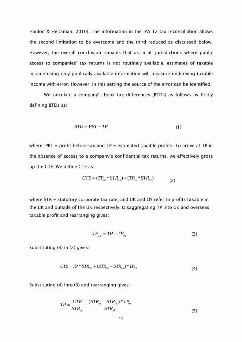
We calculate a company’s book tax differences (BTDs) as follows by firstly
defining BTDs as:
TPPBTBTD (1)
where: PBT = profit before tax and TP = estimated taxable profits. To arrive at TP in
the absence of access to a company’s confidential tax returns, we effectively gross
up the CTE. We define CTE as:
)*()*( ososukuk STRTPSTRTPCTE (2)
where STR = statutory corporate tax rate, and UK and OS refer to profits taxable in
the UK and outside of the UK respectively. Disaggregating TP into UK and overseas
taxable profit and rearranging gives:
osuk TPTPTP (3)
Substituting (3) in (2) gives:
osukosuk TPSTRSTRSTRTPCTE *)(* (4)
Substituting (4) into (3) and rearranging gives:
uk
osukos
uk STR
TPSTRSTR
STR
CTETP
*)( (5)
13
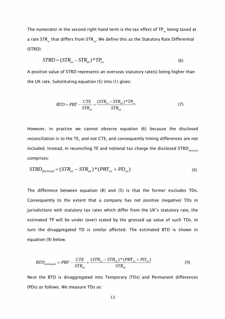
The numerator in the second right hand term is the tax effect of TPos being taxed at
a rate STRos that differs from STR
uk. We define this as the Statutory Rate Differential
(STRD):
osukos TPSTRSTRSTRD *)( (6)
A positive value of STRD represents an overseas statutory rate(s) being higher than
the UK rate. Substituting equation (5) into (1) gives:
uk
osukos
uk STR
TPSTRSTR
STR
CTEPBTBTD
*)( (7)
However, in practise we cannot observe equation (6) because the disclosed
reconciliation is to the TE, and not CTE, and consequently timing differences are not
included. Instead, in reconciling TE and notional tax charge the disclosed STRDdisclosed
comprises:
)(*)( ososukosdisclosed PDPBTSTRSTRSTRD (8)
The difference between equation (8) and (5) is that the former excludes TDs.
Consequently to the extent that a company has net positive (negative) TDs in
jurisdictions with statutory tax rates which differ from the UK’s statutory rate, the
estimated TP will be under (over) stated by the grossed up value of such TDs. In
turn the disaggregated TD is similar affected. The estimated BTD is shown in
equation (9) below.
uk
ososukos
ukesttimated STR
PDPBTSTRSTR
STR
CTEPBTBTD
)(*)( (9)
Next the BTD is disaggregated into Temporary (TDs) and Permanent differences
(PDs) as follows. We measure TDs as:
14
ukSTR
DTETD (10)
where DTE is adjusted for non-current items, as discussed above. A positive signed
TD represents temporary differences with the net effect of reducing the current year
taxable income relative to accounting income and vice versa. Finally, permanent
differences are defined as:
TDTPPBTPD (11)
A positive signed PD represents an adjustment that decreases taxable income
relative to accounting income. PDs capture non-reversing reconciling items that
arise from differences between accounting income and taxable income measures.
Data analysis
The data is initially analysed using change of sign to determine the extent to
which BTDs and their components vary over time. Subsequently, dynamic panel-data
estimation is employed to assess formally the relation between BTDs and their
lagged value. To capture heterogeneity in firm specific factors, normally a fixed
effects model could be estimated. In this setting of a short time period and large
number of companies i.e. “small T and large N”, the use of a lagged dependent
variable as an independent variable results in biased estimates of the coefficients of
the lagged variable (Nickell, 1981). Consequently, in this setting we use the Blundell
and Bond (1998) generalised method of moments (GMM) estimator.9 To remove
scale effects present when using accounting data the analysis is conducted on size
deflated variables, with book value of closing assets (BVA) acting as the deflator
(Shen and Stark, 2011).10 Descriptive statistics are also reported for variables
deflated by profit before tax (PBT), which although having a more intuitive
interpretation in linking BTD with pre-tax accounting income, may reflect scale
15
effects because of possible association between levels of pre-tax accounting income
and BTDs.,11 In testing the degree of persistence a one period autoregressive
process AR(1). An AR(1) process maximises the number of observations used in
estimation thereby leading to more robust estimations and is comparable to models
used in time series studies of accounting income and taxable income (Plesko and
Weber (2009).12 The formal model is in turn estimated for BTD and each of its three
components, PD, TD and STRD as in (12) below in the context of modelling BTD.
itit
it
it
it XPBT
BTD
PBT
BTD '1 (12)
where 'X is a vector of year dummies 2006, 2007, 2008, 2009 and 2010.13 As
discussed above, there is evidence of an association between companies’ industry
classification and their tax status, the above model is also estimated on sub
samples formed by industry group.
5. Results
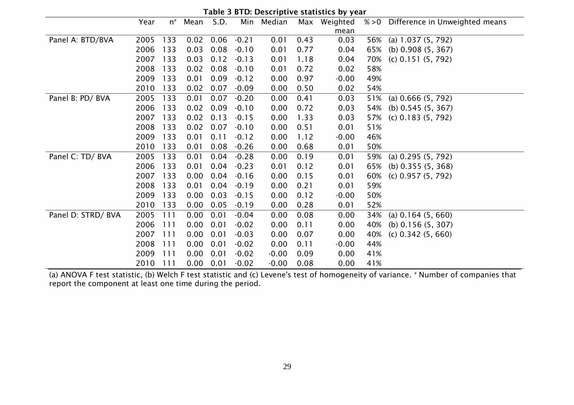
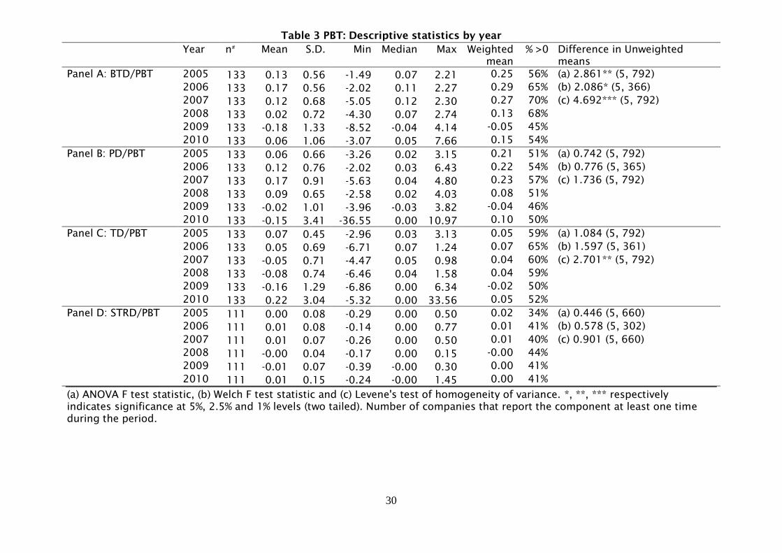
Descriptive statistics for annual BTDs and components are reported in table
3. Taking the sample as a whole, the weighted mean BTD is positive in all years
except 2009, i.e. accounting income exceeds taxable income in each of these five
years. The excess is in a narrow range of 2% to 4%. The number of companies with a
positive BTD is an increasing majority for each of first three years before falling
back over the next three years: over the six years the number ranges from to 49% to
70%. The mean un-weighted BTD is positive in the first three years and negative in
2008, 2009 and 2010.
A similar pattern exists with PDs. For each of the first three years the
weighted mean 3% is positive i.e. on average PDs increase taxable income relative to
16
accounting income, before a lower weighted mean in the remaining three years with
a minimum, negative value, in 2009. The percentage of companies with positive
PDs follows a similar trend to BTDs though closer to 50%.
There is less variation in the weighted mean TD which is 1% in five years and
-1% in the remaining year, 2009. On average the effect of TDs is to increase taxable
profits relative to accounting profits. The range of the percentage of companies
with positive TDs is 50% to 65%. While all companies have PDs and TDs a reduced
number have STRDs. The weighted mean is positive in all six years indicating that
on average overseas statutory rates are higher than the UK rate. However, at the
firm level this holds for only a minority of companies ranging, from 34% in 2005 to
44% in 2008. For the majority, overseas profits are taxed at a lower rate than the UK
rate.
To examine the stability of the magnitudes of BTDs and their components,
the differences between the unweighted means across years were analysed using
ANOVA. The results are reported in the final column of Table 3 indicate no
significant differences, suggestive of persistency at the sample level.14
XXX Insert Tables 3 and 4 about here XXX
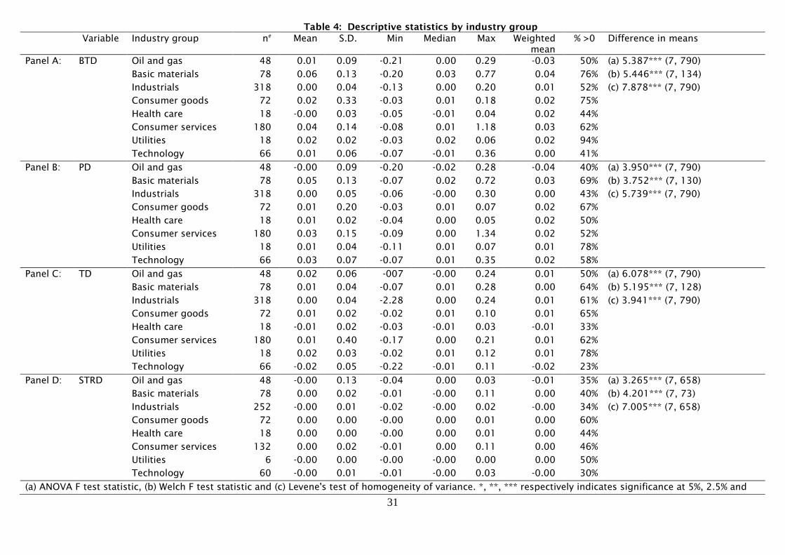
When examined by industry category, there is some evidence of strong
industry effect in BTDs, see panel A table 4. The number of companies with positive
BTDs ranges from 41% in the Technology sector to 94% in Utilities. In contrast,
several industries lie in what can be considered an “inconclusive” range, with Oil
and gas with 50% to Industrials with 52%. Similar mixed patterns of persistence in
certain industries and lack of it in others occurs with PDs and TDs in panels B and
C. The STRD component shows the highest level of consistency across industries
17
with all but two industries, Consumer Goods and Utilities, having a sizeable minority
of companies with positive STRDs.
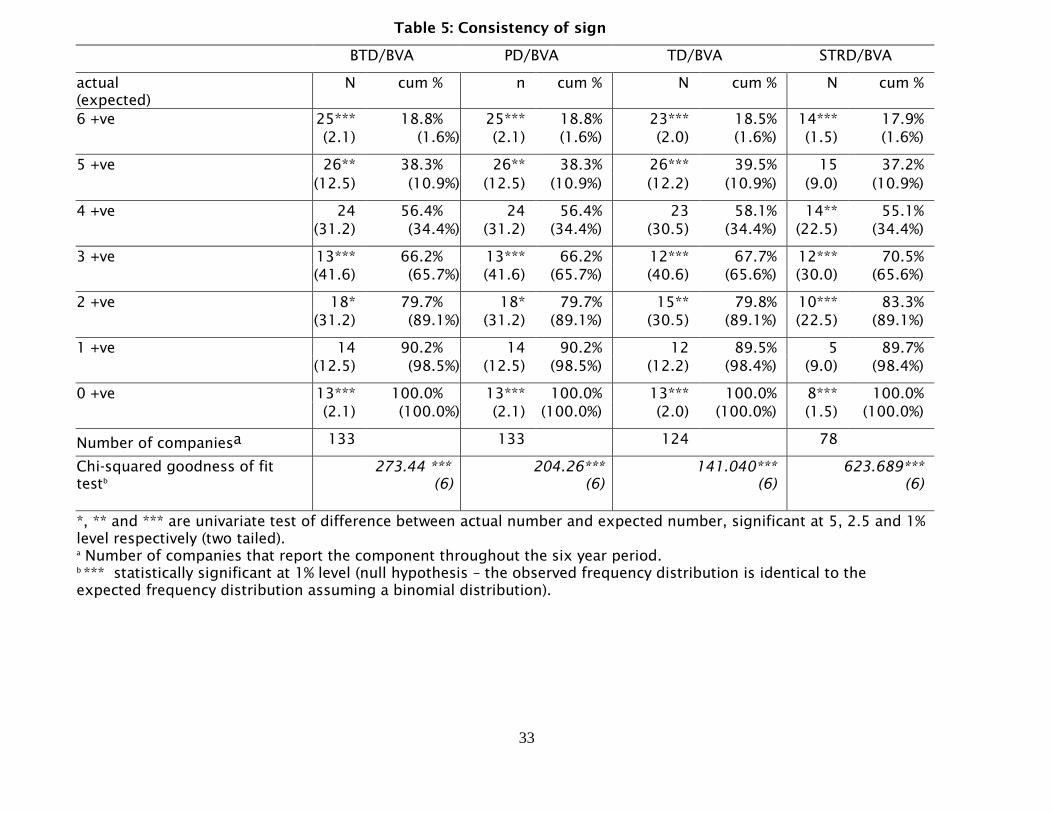
The above analysis examines BTDs and their components on a sample wide
basis and therefore individual firm variation may be lost in aggregation. To examine
company level variation, table 5 compares the expected and actual frequency of the
sign of BTDs and their components. This is a direct test of consistency of effect.
The first row reports the expected and actual frequency of the number of
companies whose BTDs are positive in all six years of data, row two shows similar
data for companies with five occurrences of positive BTDs (and therefore one year
of negative BTD), and so on. Assuming independence across time the expected
values are generated using a binomial distribution with the probability of a negative
(positive) sign = 0.5. At the extreme position of 6 positive (negative) signed BTDs
i.e. no changes in sign, the actual number, 25 (13) is significantly greater than the
expected number of 2.1 (2.1) at the 1% level in both cases. In the next case, one
“change” of sign i.e. five positive or five negative BTDs, the actual number is greater
than expected in both cases, though the difference is only statistically significant in
the former case. Overall, 58.7% of companies experience at least five positive (or
five negative signed BTDs in the six-year period with the expected level is 29.2%.
The three remaining frequency categories have lower than expected frequencies as
a corollary to the higher than expected frequencies in the more “extreme” positions.
XXX Insert Table 5 about here XXX
The component PD exhibits a similar level of persistence. Of the 133
companies, 38.3% (51) have at least five positive signed PDs and 20.3% (27) have at
least five negative signed PDs in the six-year period compared with an expected
10.9% for each category. The component TD also shows consistency with 39.5% (49)
18
of companies having at least five positive signed TDs, and 20.2% (25) with at least
five negative signed TDs in the six-year period. This compares with an expected
rate of 10.9% for five or more positive or negative signed TDs. The component STRD
is generally similar to PD in terms of consistency of sign. Of the 78 companies
which reported STRDs, 37.2% (29) have at least five positive STRDs while 13 (16.7%)
reported at least five negative STRDs compared with an expected percentage of
10.9% in each case. Overall, there is strong evidence of persistence; the null
hypothesis of the frequency following a binomial distribution is rejected for BTD
and each of its components as indicated by the significant chi-squared goodness of
fit tests reported at the foot of table 5.
XXX Insert Table 6 about here XXX
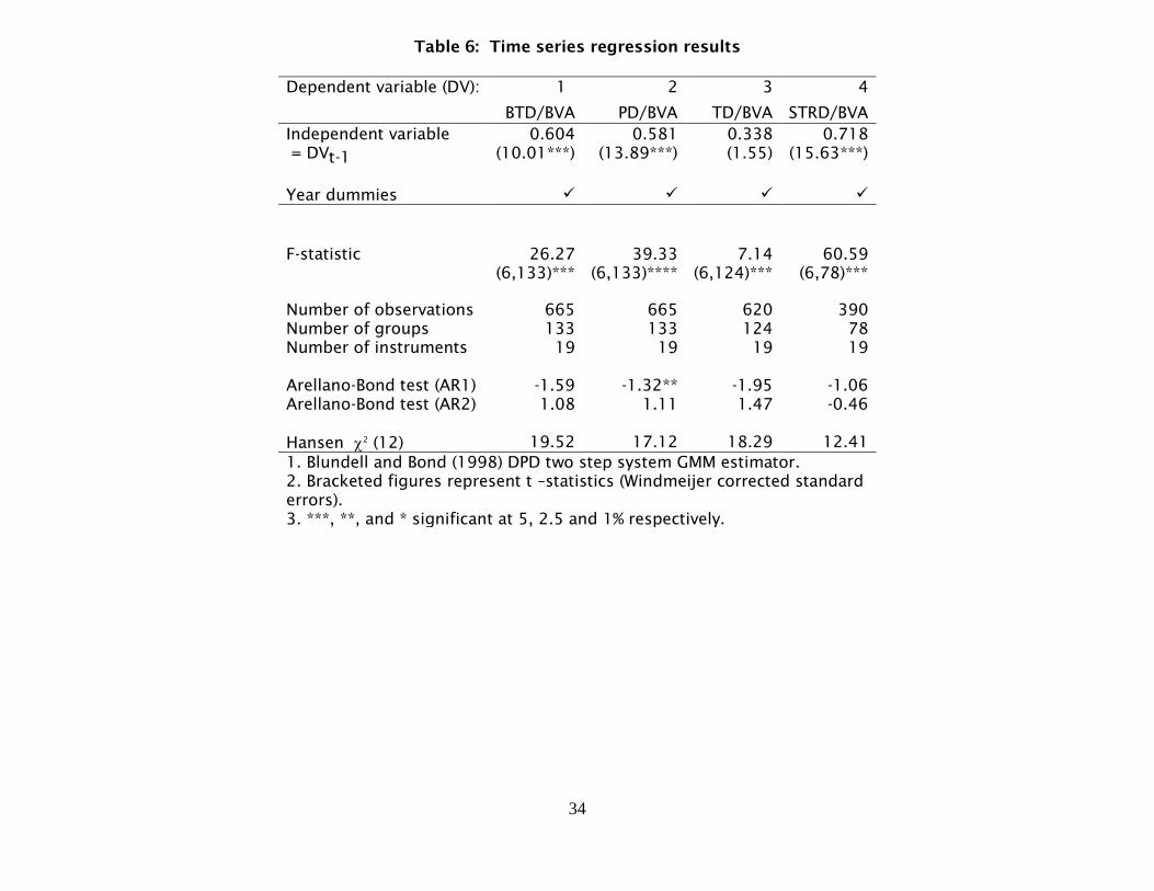
Table 6 summarises a series of time series estimations of the relation
between BTDs and its one -period lag, the results are given in columns 1. In
columns 2, 3 and 4 similar estimations are reported for PDs, TDs and STRDs
respectively. In each of the estimations the diagnostic tests are satisfied: the
Hansen test of instrument over-identification is satisfactory with an insignificant
test statistic along with insignificant AR (2) errors. For BTD, PD and STRD there is a
significant, stable, relation over time with the estimated coefficients on the lagged
terms within the range ±1.00. The lagged variable TD is also positive though
statistically insignificant. Of the three components, STRDs has the highest level of
persistence when measured by the size of the coefficients with TDs being the least.
The coefficients for the three components are statistically significantly different
from each at the 1% level.
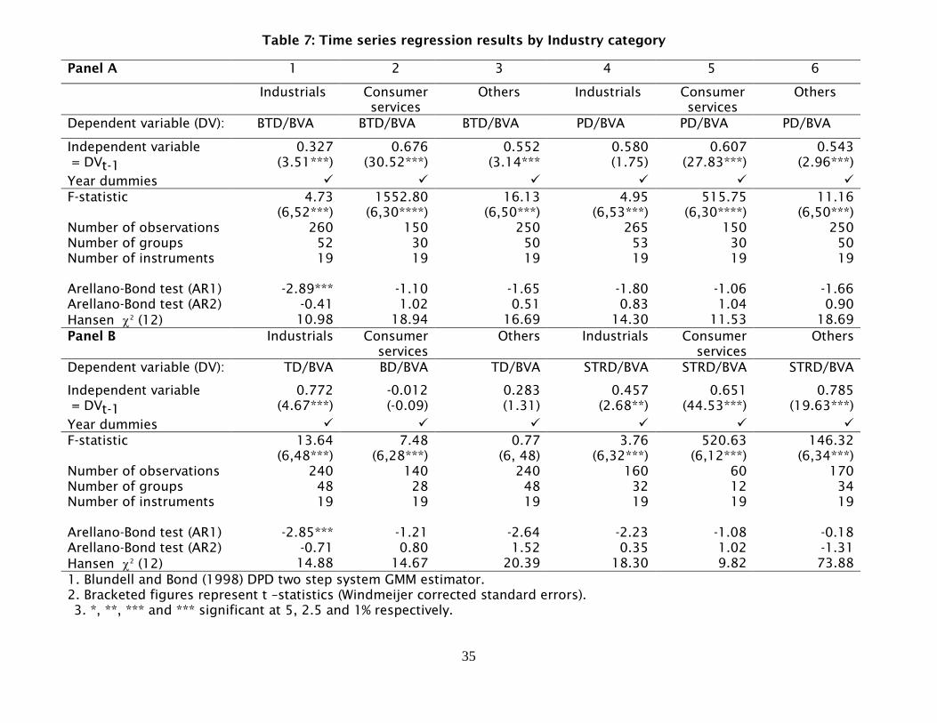
To assess whether the above sample wide results are stable across individual
industrial groups, we re-estimate the models on three subsamples of companies.
19
Although there are eight industrial categories represented in the sample, see table
2, there are insufficient number of observations within some of these categories to
estimate each individually. Instead, the sample is disaggregated into the two largest
industry categories Industrials, and Consumer Services with 318 and 180
observations respectively with the remaining categories collapsed into a third
group, referred to as Others with 300 observations. The results are summarised in
Table 7.
XXX Insert Table 7 about here XXX
Each of the four estimated models satisfies the required diagnostic tests with
insignificant Hansen test statistic and insignificant AR(2) errors. The coefficient for
the lagged BTD variable is statistically significant at the 1% level in all three industry
groups and ranges from 0.327 to 0.676, see columns 1, 2 and 3.15 With each
coefficient being statistically significantly different from both zero and each other,
this suggests the initial finding of persistence is general to the full sample, rather
than being driven by a sub category of observations, and, that the degree of
persistence varies by industry group. The source of the persistence varies with PDs
exhibiting significance in both Consumer Services and Others and TDs in
Industrials. Only for STRD is there significant persistence for in all three industry
groups.
6. Discussion and conclusions
This paper reports the results of an initial investigation into the behaviour of
BTDs using hand-collected tax reconciliation data drawn from a panel of UK quoted
non-financial companies during the period 2005 – 2010.
20
Overall, the various analyses can be summarised as follows. There is
evidence of consistency in the sign of BTDs and their components in a limited
number of industry groups (table 4) though in the majority of groups, there is no
dominate trend. Within companies, goodness of fits tests are rejected (table 5)
indicative of consistency of sign. However, this consistency does not apply to all
companies. For example, only 79 companies (59.4%) had either five or more
positive or negative BTDs in the sample period (table 5). Further, formal time series
models indicate the degree of persistence both varies by type of BTD and across
industry. In the context of interpreting the underlying sources of BTDs, STRD has
the significantly the highest level of persistence (0.718, table 6) suggesting taxation
as important motivating factor. With the majority of companies face a lower
overseas statutory rate compared to the UK rate the ability to maintain the STRD
effect over time is consistent with an underlying tax motivation. Though the
presence of a number of companies consistently facing the reverse relative
magnitude of overseas and UK statutory rates indicates non-tax benefits influence
location or income recognition decisions.
In the absence of full disclosures on the nature of PDs it is difficult to
determine an underlying motivation. However, the observation that on average only
51.5% of PDs were positive over the six year period (average of percentages in table
3 panel B) indicates that a significant number of PDs do not represent simple “add
backs” of non-qualifying accounting deductions. A significant proportion of the
adjustments are of income recognised for accounting income but which is non-
taxable, this would be consistent with “aggressive” financial reporting (Hanlon &
Slemrod, 2009).
The relative low persistence of TDs (0.338, table 3) is unexpected if TDs are
driven by systematic earnings management over several periods. Instead, the low
value is consistent with the effect of new originating differences being offset by the
21
inevitable reversal of earlier timing differences, a more “mechanical” process. When
for example levels of capital expenditure qualifying for capital allowances increase
over time (net) TDs would persist though any reduction in expenditure could result
in a reversal of effect as appears to be the case in 2009 (see table 3).
In using BTDs to assess a company’s taxation behaviour these results imply
users of tax disclosures should attempt to determine the nature of the BTD and
observe their properties over a number of periods. A similar approach should be
adopted in using BTDs as a measure of earnings quality. Further research could
investigate the source(s) of cross-sectional variation in the level of persistence
although the extent to which this could be done using currently publically disclosed
tax related information is an empirical question.
Notes: 1 Prior to 2005 UK companies were able to provide deferred tax on a partial
provisioning method which limited the ability to examine changes over time
without access to private information on forecast profits, capital expenditure etc.
(Holland and Jackson, 2004).
2 ETRs and BTDs are related in that ETRs are the after tax equivalent of (before tax)
BTDs.
3 Long run measures “avoids much of the mismatch of cash taxes and earnings”
(Hanlon and Heitzman 2010), as discussed subsequently we focus on the accrued
tax charge and exclude prior year adjustments to minimise this effect.
4 The treatment would however effect the composition of the total tax expense. i.e.
between current and deferred tax charges.
22
5 ETR is defined as the ratio of current tax expense relative to the accounting profit
before tax. The ETR is the after tax effect of the pre-tax or gross book tax-
difference.
6 IAS 12 allows uses of domestic rate or the weighted average rate of the
jurisdictions in which the company operates. In all company year end
reconciliations included in the sample the domestic (UK) statutory rate was used.
7 See footnote 5.
8 The effect of tax credits for expenditure on e.g. research and development
expenditure are also adjusted as they are required to be disclosed.
9 Estimated using the xtabond2 command in Stata, see Roodman (2009).
10 While Shen and Stark (2011) examine deflator properties in the context of
valuation models such models utilise financial statement based data as in this
study and therefore it is reasonable to apply their conclusion in this setting.
11 The results of the BVA and PBT deflated data are qualitatively the same. When
deflating by PBT, the resulting measure has an obvious interpretation in stating
the BTD relative to PBT. However, to reduce the effect of any relation between the
level of PBT and BTD, the BVA deflator is used (Plesko and Weber 2009).
12 Untabulated results based on an AR(2) process show qualitatively similar results
to those using the AR(1) specification.
13 The use of time dummies is recommended by Roodman (2009) to assist in
meeting the assumption that idiosyncratic disturbances are uncorrelated across
observations.
14 In the absence of homogeneous variances across years, the Welch robustness test
is also reported as appropriate.
15 With two exceptions the difference in regression coefficients between each pair
of industry groups is significant at the 1% level for each set of comparison i.e.
BTD, PD, TD and STRD, for example, the comparison of _BTD_Industrialst-1 with

23
_BTD_Consumer_Servicest-1 etc. The two exceptions are the insignificant
difference between _PD_Industrialst-1and _PD_Consumer_Cervicest-1 and the
insignificant difference between _PD_Industrialst-1and _PD_Otherst-1T-
statistics available from authors upon request.

24
References
Abdul Wahab, N. S., Holland, K. (2012). Tax planning, corporate governance and equity value. The British Accounting Review, 44(2), 111-124. Altshuler, R., Auerbach, A. J., Cooper, M., Knittel (2009). Understanding U.S. corporate tax losses. In Brown, J. R., Poterba, J. (Eds.) Tax Policy and the Economy. Chicago: University of Chicago Press, 73-122. Blaylock, B., Shevlin, T., Wilson, R. (2012). Tax avoidance, large positive temporary book-tax differences, and earnings persistence. The Accounting Review, 87(1), 91-120. Blundell, R., Bond, S. (1998). Initial conditions and moment restrictions in dynamic panel data models. Journal of econometrics, 87(1), 115-143. Boynton, C., Mills, L. (2004). The evolving Schedule M–3: A new era of corporate show and tell? National Tax Journal, 757-772. Bradley, M., Jarrell, G. A., Kim, E. H. (1984). On the existence of an optimal capital structure: Theory and evidence. The Journal of Finance, 39(3), 857-878. Bucovetsky, S., Haufler, A. (2008). Tax competition when firms choose their organizational form: Should tax loopholes for multinationals be closed? Journal of International Economics, 74(1), 188-201. Chen, L. H., Dhaliwal, D. S., Trombley, M. A. (2012). Consistency of book-tax differences and the information content of earnings. Journal of the American Taxation Association, 34(2), 93-116. Christian Aid (2012). Tax Dodging Costs Lives, available on the internet at http://www.christianaid.org.uk/ActNow/trace-the-tax/ Accessed 07.07.13. Desai, M. (2005). The degradation of corporation profits. Journal of Economic Perspectives 19 (Fall): 171-192. Devereux, M. P., Lockwood, B., Redoano, M. (2008). Do countries compete over corporate tax rates? Journal of Public Economics, 92(5-6), 1210-1235. Donohoe, M. P., McGill, G. A. (2011). The effects of increased book-tax difference tax return disclosures on firm valuation and behavior. Journal of the American Taxation Association, 33(2), 35-65. Donohoe, M., McGill, G., Outslay, E. (2012). Through a glass darkly: What can we learn about a US multinational corporation's international operations from its financial statement disclosures? National Tax Journal, 65(4), 961-984. Dyreng, S., Hanlon, M., Maydew, E. L. (2008). Long-run corporate tax avoidance. The Accounting Review, 83(1), 61-82. Dyreng, S., Hanlon, M., Maydew, E. L. (2010). The effects of executives on corporate tax avoidance. The Accounting Review, 85(4), 1163-1189.

25
Erickson, M., Hanlon, M., Maydew, E., 2004. How much will firms pay for earnings that do not exist? Evidence of taxes paid on allegedly fraudulent earnings. The Accounting Review, 79, 387–408 EU (2013). Tackling Tax Avoidance: Commission Tightens Key EU Corporate Tax Rules, available on the internet at http://europa.eu/rapid/press-release_IP-13-1149_en.htm Accessed 16.01.14. Frank, M. M., Lynch, L. J., Rego, S. O. (2009). Tax reporting aggressiveness and its relation to aggressive financial reporting. The Accounting Review, 84(2), 467-496. Graham, J. R., Raedy, J. S., Shackelford, D. A. (2012). Research in accounting for income taxes. Journal of Accounting and Economics, 53(1-2), 412-434. Grieson, R. E., Hamovitch, W., Levenson, A. M., Morgenstern, R. D. (1977). The effect of business taxation on the location of industry. Journal of Urban Economics, 4(2), 170-185. Hanlon, M. (2003). What can we infer about a firm’s taxable income from its financial statements? National Tax Journal, 56(4), 831–863. Hanlon, M. (2005). The persistence and pricing of earnings, accruals, and cash flows when firms have large book-tax differences. Accounting Review, 80(1), 137-166. Hanlon, M., Heitzman, S. (2010). A review of tax research. Journal of Accounting and Economics, 50(2), 127-178. Hanlon, M., Maydew, E. L., Shevlin, T. (2008). An unintended consequence of book-tax conformity: A loss of earnings informativeness. Journal of Accounting and Economics, 46(2), 294-311. Hanlon, M., Slemrod, J. B. (2009). What does tax aggressiveness signal? Evidence from stock price reactions to news about tax shelter involvement. Journal of Public Economics, 93(1-2), 126-141. Harberger, A. C. (1959). The corporation income tax: An empirical appraisal. Tax Revision Compendium, 1, 231-250. Hasseldine, J., Holland, K. M. and Van der Rijt, P. G. A. (2012). Companies and taxes in the UK: Actors, actions, consequences and responses. eJournal of Tax Research, 10(3), 532–551. HMRC (2013). The General Anti-Abuse Rule, available on the internet at www.hmrc.gov.uk/avoidance/gaar.htm Accessed 16.01.14. Holland, K. (1998). Accounting policy choice: The relationship between corporate tax burdens and company size. Journal of Business Finance & Accounting, 25(3 & 4), 265-288. Holland, K. M., Jackson, R. H. G. (2004). Earnings management and deferred tax. Accounting and Business Research. 34(2), 101 – 123. IASB (2010). International Accounting Standard 12 "Income Taxes", available on the internet at http://www.ifrs.org/Documents/IAS12.pdf Accessed 07.07.13.

26
Kim, K. A., Limpaphayom, P. (1998). Taxes and firm size in pacific-basin emerging economies. Journal of International Accounting, Auditing and Taxation, 7(1), 47-68. Kovenock, D., Phillips, G. M. (1997). Capital structure and product market behavior: An examination of plant exit and investment decisions. Review of Financial Studies, 10(3), 767-803. Maydew, E. L., Shackelford, D. A. (2007). The changing role of auditors in corporate tax planning. In Auerbach, A. J., Hines, J. R., Slemrod, J. (Eds.) Taxing Corporate Income in the 21st Century. New York: Cambridge University Press, 307-337. McIntyre, R. S., Nguyen, T. D. C. (2000). Corporate income taxes in the 1990s. Institute on Taxation and Economic Policy, 1-60. New Statesman (2011). Tax Avoidance Costs UK Economy £69.9 Billion a Year, available on the internet at http://www.newstatesman.com/blogs/the-staggers/2011/11/tax-avoidance-justice-network Accessed 07.07.13. Nickell, S. (1981). Biases in dynamic models with fixed effects. Econometrica: Journal of the Econometric Society, 49(6), 1417-1426. OECD (2013). Closing Tax Gaps - OECD Launches Action Plan on Base Erosion and Profit Shifting, available on the internet at www.oecd.org/newsroom/closing-tax-gaps-oecd-launches-action-plan-on-base-erosion-and-profit-shifting.htm Accessed 16.01.2014. Omer, T., Molloy, K., Ziebart, D. (1993). An investigation of the firm size-effective tax rate relation in the 1980s. Journal of Accounting, Auditing, and Finance, 8(2), 167-182. Phillips, J. D. (2003). Corporate tax-planning effectiveness: The role of compensation-based incentives. The Accounting Review, 78(3), 847-874. Plesko, G. A., Weber, D. P. (2009). The time-series properties of book and taxable income, Proceedings of the Annual Conference on Taxation, (Columbus: National Tax Association - Tax Institute of America). Public Accounts Committee (2012). Public Accounts Committee - Nineteenth Report, London, available at: www.publications.parliament.uk/pa/cm201213/cmselect/cmpubacc/716/71602.htm Accessed 16.01.2014. Raedy, J. S., Seidman, J., Shackelford, D. A. (2011). Is there information content in the tax footnote? Research paper series 23rd Annual American Taxation Association Mid-Year Meeting. Roodman, D. (2009). How to do xtabond2: An introduction to difference and system GMM in Stata. Stata Journal, 9(1), 86-136. Schmidt, A. P. (2006). The persistence, forecasting, and valuation implications of the tax change component of earnings. The Accounting Review, 81(3), 589-616.

27
Shackelford, D. A., Slemrod, J., Sallee, J. M. (2011). Financial reporting, tax, and real decisions: Toward a unifying framework. International Tax and Public Finance, 18(4), 461-494. Shen, Y., Stark, A. W. (2011). Evaluating the Effectiveness of Model Specifications and Estimation Approaches for Empirical Accounting-Based Valuation Models (July 18, 2011). Forthcoming in Accounting and Business Research 2014, available at SSRN: http://ssrn.com/abstract=1888386 or http://dx.doi.org/10.2139/ssrn.1888386 Accessed 16.01.2014. Sloan, R. G. (1996). Do stock prices fully reflect information in accruals and cash flows about future earnings? The Accounting Review, 71(3), 289-315. Tang, T., Firth, M. (2011). Can book-tax differences capture earnings management and tax management? Empirical evidence from China. The International Journal of Accounting, 46(2), 175-204. The Guardian (2009). Firms' Secret Tax Avoidance Schemes Cost UK Billions: Investigation into the Complex and Confidential World of Tax, available on the internet at http://www.guardian.co.uk/business/2009/feb/02/tax-gap-avoidance. Accessed 07.07.13. Trade Union Congress (2009). The Missing Billions the UK Tax Gap, available on the internet at www.tuc.org.uk/touchstone/Missingbillions/1missingbillions.pdf Accessed 07.07.13. UK Uncut (2010). Big Society Revenue & Customs, available on the internet at http://www.ukuncut.org.uk/targets Accessed 07.07.13. Whiting, J. (2006). Tax and Accounting 2006, British Tax Review, 3, 267 - 281. Wilson, R. (2009). An examination of corporate tax shelter participants. The Accounting Review, 84(3), 969-999.
28
Figure 1: Accounting and taxation processes
Cash flow
from operations
+ Net
accruals =
Pre-tax Accounting
earnings +
Net book tax differences
(BTDs) =
Taxable Income
Table 1: Sample reconciliation
Details n
Non-financial public listed companies (listed throughout the period) 2490
At least one year of annual report is not available (462)
At least one of the accounting periods is more than 12 months (552)
Extreme value of effective tax rates (-1>ETR>1) (57)
Negative profit before tax (143)
Unbalance data (478)
Total sample 798
Table 2: Distribution of sample by industry
Details Firm-year (n=798) %
Oil and gas 48 6.01
Basic materials 78 9.77
Industrials 318 39.85
Consumer goods 72 9.02
Health care 18 2.26
Consumer services 180 22.56
Utilities 18 2.26
Technology 66 8.27
Total (133 companies * 6 year ends) 798 100
Note: Based on FT-SE Industry Classifications.
29
Table 3 BTD: Descriptive statistics by year
Year n# Mean S.D. Min Median Max Weighted mean
% >0 Difference in Unweighted means
Panel A: BTD/BVA 2005 133 0.02 0.06 -0.21 0.01 0.43 0.03 56% (a) 1.037 (5, 792)
2006 133 0.03 0.08 -0.10 0.01 0.77 0.04 65% (b) 0.908 (5, 367)
2007 133 0.03 0.12 -0.13 0.01 1.18 0.04 70% (c) 0.151 (5, 792)
2008 133 0.02 0.08 -0.10 0.01 0.72 0.02 58% 2009 133 0.01 0.09 -0.12 0.00 0.97 -0.00 49% 2010 133 0.02 0.07 -0.09 0.00 0.50 0.02 54% Panel B: PD/ BVA 2005 133 0.01 0.07 -0.20 0.00 0.41 0.03 51% (a) 0.666 (5, 792)
2006 133 0.02 0.09 -0.10 0.00 0.72 0.03 54% (b) 0.545 (5, 367)
2007 133 0.02 0.13 -0.15 0.00 1.33 0.03 57% (c) 0.183 (5, 792)
2008 133 0.02 0.07 -0.10 0.00 0.51 0.01 51% 2009 133 0.01 0.11 -0.12 0.00 1.12 -0.00 46% 2010 133 0.01 0.08 -0.26 0.00 0.68 0.01 50% Panel C: TD/ BVA 2005 133 0.01 0.04 -0.28 0.00 0.19 0.01 59% (a) 0.295 (5, 792)
2006 133 0.01 0.04 -0.23 0.01 0.12 0.01 65% (b) 0.355 (5, 368)
2007 133 0.00 0.04 -0.16 0.00 0.15 0.01 60% (c) 0.957 (5, 792)
2008 133 0.01 0.04 -0.19 0.00 0.21 0.01 59% 2009 133 0.00 0.03 -0.15 0.00 0.12 -0.00 50% 2010 133 0.00 0.05 -0.19 0.00 0.28 0.01 52% Panel D: STRD/ BVA 2005 111 0.00 0.01 -0.04 0.00 0.08 0.00 34% (a) 0.164 (5, 660)
2006 111 0.00 0.01 -0.02 0.00 0.11 0.00 40% (b) 0.156 (5, 307)
2007 111 0.00 0.01 -0.03 0.00 0.07 0.00 40% (c) 0.342 (5, 660)
2008 111 0.00 0.01 -0.02 0.00 0.11 -0.00 44% 2009 111 0.00 0.01 -0.02 -0.00 0.09 0.00 41% 2010 111 0.00 0.01 -0.02 -0.00 0.08 0.00 41%
(a) ANOVA F test statistic, (b) Welch F test statistic and (c) Levene's test of homogeneity of variance. # Number of companies that report the component at least one time during the period.
30
Table 3 PBT: Descriptive statistics by year
Year n# Mean S.D. Min Median Max Weighted mean
% >0 Difference in Unweighted means
Panel A: BTD/PBT 2005 133 0.13 0.56 -1.49 0.07 2.21 0.25 56% (a) 2.861** (5, 792)
2006 133 0.17 0.56 -2.02 0.11 2.27 0.29 65% (b) 2.086* (5, 366)
2007 133 0.12 0.68 -5.05 0.12 2.30 0.27 70% (c) 4.692*** (5, 792)
2008 133 0.02 0.72 -4.30 0.07 2.74 0.13 68% 2009 133 -0.18 1.33 -8.52 -0.04 4.14 -0.05 45% 2010 133 0.06 1.06 -3.07 0.05 7.66 0.15 54% Panel B: PD/PBT 2005 133 0.06 0.66 -3.26 0.02 3.15 0.21 51% (a) 0.742 (5, 792)
2006 133 0.12 0.76 -2.02 0.03 6.43 0.22 54% (b) 0.776 (5, 365)
2007 133 0.17 0.91 -5.63 0.04 4.80 0.23 57% (c) 1.736 (5, 792)
2008 133 0.09 0.65 -2.58 0.02 4.03 0.08 51% 2009 133 -0.02 1.01 -3.96 -0.03 3.82 -0.04 46% 2010 133 -0.15 3.41 -36.55 0.00 10.97 0.10 50% Panel C: TD/PBT 2005 133 0.07 0.45 -2.96 0.03 3.13 0.05 59% (a) 1.084 (5, 792)
2006 133 0.05 0.69 -6.71 0.07 1.24 0.07 65% (b) 1.597 (5, 361)
2007 133 -0.05 0.71 -4.47 0.05 0.98 0.04 60% (c) 2.701** (5, 792)
2008 133 -0.08 0.74 -6.46 0.04 1.58 0.04 59% 2009 133 -0.16 1.29 -6.86 0.00 6.34 -0.02 50% 2010 133 0.22 3.04 -5.32 0.00 33.56 0.05 52% Panel D: STRD/PBT 2005 111 0.00 0.08 -0.29 0.00 0.50 0.02 34% (a) 0.446 (5, 660)
2006 111 0.01 0.08 -0.14 0.00 0.77 0.01 41% (b) 0.578 (5, 302)
2007 111 0.01 0.07 -0.26 0.00 0.50 0.01 40% (c) 0.901 (5, 660)
2008 111 -0.00 0.04 -0.17 0.00 0.15 -0.00 44% 2009 111 -0.01 0.07 -0.39 -0.00 0.30 0.00 41% 2010 111 0.01 0.15 -0.24 -0.00 1.45 0.00 41%
(a) ANOVA F test statistic, (b) Welch F test statistic and (c) Levene's test of homogeneity of variance. *, **, *** respectively indicates significance at 5%, 2.5% and 1% levels (two tailed). Number of companies that report the component at least one time during the period.
31
Table 4: Descriptive statistics by industry group
Variable Industry group n# Mean S.D. Min Median Max Weighted mean
% >0 Difference in means
Panel A: BTD Oil and gas 48 0.01 0.09 -0.21 0.00 0.29 -0.03 50% (a) 5.387*** (7, 790)
Basic materials 78 0.06 0.13 -0.20 0.03 0.77 0.04 76% (b) 5.446*** (7, 134)
Industrials 318 0.00 0.04 -0.13 0.00 0.20 0.01 52% (c) 7.878*** (7, 790)
Consumer goods 72 0.02 0.33 -0.03 0.01 0.18 0.02 75%
Health care 18 -0.00 0.03 -0.05 -0.01 0.04 0.02 44%
Consumer services 180 0.04 0.14 -0.08 0.01 1.18 0.03 62%
Utilities 18 0.02 0.02 -0.03 0.02 0.06 0.02 94%
Technology 66 0.01 0.06 -0.07 -0.01 0.36 0.00 41%
Panel B: PD Oil and gas 48 -0.00 0.09 -0.20 -0.02 0.28 -0.04 40% (a) 3.950*** (7, 790)
Basic materials 78 0.05 0.13 -0.07 0.02 0.72 0.03 69% (b) 3.752*** (7, 130)
Industrials 318 0.00 0.05 -0.06 -0.00 0.30 0.00 43% (c) 5.739*** (7, 790)
Consumer goods 72 0.01 0.20 -0.03 0.01 0.07 0.02 67%
Health care 18 0.01 0.02 -0.04 0.00 0.05 0.02 50%
Consumer services 180 0.03 0.15 -0.09 0.00 1.34 0.02 52%
Utilities 18 0.01 0.04 -0.11 0.01 0.07 0.01 78%
Technology 66 0.03 0.07 -0.07 0.01 0.35 0.02 58%
Panel C: TD Oil and gas 48 0.02 0.06 -007 -0.00 0.24 0.01 50% (a) 6.078*** (7, 790)
Basic materials 78 0.01 0.04 -0.07 0.01 0.28 0.00 64% (b) 5.195*** (7, 128)
Industrials 318 0.00 0.04 -2.28 0.00 0.24 0.01 61% (c) 3.941*** (7, 790)
Consumer goods 72 0.01 0.02 -0.02 0.01 0.10 0.01 65%
Health care 18 -0.01 0.02 -0.03 -0.01 0.03 -0.01 33%
Consumer services 180 0.01 0.40 -0.17 0.00 0.21 0.01 62%
Utilities 18 0.02 0.03 -0.02 0.01 0.12 0.01 78%
Technology 66 -0.02 0.05 -0.22 -0.01 0.11 -0.02 23%
Panel D: STRD Oil and gas 48 -0.00 0.13 -0.04 0.00 0.03 -0.01 35% (a) 3.265*** (7, 658)
Basic materials 78 0.00 0.02 -0.01 -0.00 0.11 0.00 40% (b) 4.201*** (7, 73)
Industrials 252 -0.00 0.01 -0.02 -0.00 0.02 -0.00 34% (c) 7.005*** (7, 658)
Consumer goods 72 0.00 0.00 -0.00 0.00 0.01 0.00 60%
Health care 18 0.00 0.00 -0.00 0.00 0.01 0.00 44%
Consumer services 132 0.00 0.02 -0.01 0.00 0.11 0.00 46%
Utilities 6 -0.00 0.00 -0.00 -0.00 0.00 0.00 50%
Technology 60 -0.00 0.01 -0.01 -0.00 0.03 -0.00 30%
(a) ANOVA F test statistic, (b) Welch F test statistic and (c) Levene's test of homogeneity of variance. *, **, *** respectively indicates significance at 5%, 2.5% and

32
1% levels (two tailed).# Number of companies that report the component at least one time during the period.
33
Table 5: Consistency of sign
BTD/BVA PD/BVA TD/BVA STRD/BVA
actual (expected)
N cum % n cum % N cum % N cum %
6 +ve 25*** 18.8% 25*** 18.8% 23*** 18.5% 14*** 17.9% (2.1) (1.6%) (2.1) (1.6%) (2.0) (1.6%) (1.5) (1.6%)
5 +ve 26** 38.3% 26** 38.3% 26*** 39.5% 15 37.2% (12.5) (10.9%) (12.5) (10.9%) (12.2) (10.9%) (9.0) (10.9%)
4 +ve 24 56.4% 24 56.4% 23 58.1% 14** 55.1% (31.2) (34.4%) (31.2) (34.4%) (30.5) (34.4%) (22.5) (34.4%)
3 +ve 13*** 66.2% 13*** 66.2% 12*** 67.7% 12*** 70.5% (41.6) (65.7%) (41.6) (65.7%) (40.6) (65.6%) (30.0) (65.6%)
2 +ve 18* 79.7% 18* 79.7% 15** 79.8% 10*** 83.3% (31.2) (89.1%) (31.2) (89.1%) (30.5) (89.1%) (22.5) (89.1%)
1 +ve 14 90.2% 14 90.2% 12 89.5% 5 89.7% (12.5) (98.5%) (12.5) (98.5%) (12.2) (98.4%) (9.0) (98.4%)
0 +ve 13*** 100.0% 13*** 100.0% 13*** 100.0% 8*** 100.0% (2.1) (100.0%) (2.1) (100.0%) (2.0) (100.0%) (1.5) (100.0%)
Number of companiesa 133 133 124 78
Chi-squared goodness of fit testb
273.44 *** (6)
204.26*** (6)
141.040*** (6)
623.689*** (6)
*, ** and *** are univariate test of difference between actual number and expected number, significant at 5, 2.5 and 1% level respectively (two tailed). a Number of companies that report the component throughout the six year period. b *** statistically significant at 1% level (null hypothesis – the observed frequency distribution is identical to the expected frequency distribution assuming a binomial distribution).
34
Table 6: Time series regression results
Dependent variable (DV): 1 2 3 4
BTD/BVA PD/BVA TD/BVA STRD/BVA Independent variable = DVt-1
0.604 (10.01***)
0.581 (13.89***)
0.338 (1.55)
0.718 (15.63***)
Year dummies
F-statistic 26.27
(6,133)*** 39.33
(6,133)**** 7.14
(6,124)*** 60.59
(6,78)***
Number of observations 665 665 620 390 Number of groups 133 133 124 78 Number of instruments 19 19 19 19 Arellano-Bond test (AR1)
-1.59
-1.32**
-1.95
-1.06
Arellano-Bond test (AR2) 1.08 1.11 1.47 -0.46 Hansen 2 (12)
19.52
17.12
18.29
12.41
1. Blundell and Bond (1998) DPD two step system GMM estimator. 2. Bracketed figures represent t –statistics (Windmeijer corrected standard errors). 3. ***, **, and * significant at 5, 2.5 and 1% respectively.
35
Table 7: Time series regression results by Industry category
Panel A 1 2 3 4 5 6
Industrials Consumer services
Others Industrials Consumer services
Others
Dependent variable (DV): BTD/BVA BTD/BVA BTD/BVA PD/BVA PD/BVA PD/BVA
Independent variable = DVt-1
0.327 (3.51***)
0.676 (30.52***)
0.552 (3.14***
0.580 (1.75)
0.607 (27.83***)
0.543 (2.96***)
Year dummies F-statistic 4.73
(6,52***) 1552.80
(6,30****) 16.13
(6,50***) 4.95
(6,53***) 515.75
(6,30****) 11.16
(6,50***) Number of observations 260 150 250 265 150 250 Number of groups 52 30 50 53 30 50 Number of instruments 19 19 19 19 19 19 Arellano-Bond test (AR1)
-2.89***
-1.10
-1.65
-1.80
-1.06
-1.66
Arellano-Bond test (AR2) -0.41 1.02 0.51 0.83 1.04 0.90 Hansen 2 (12) 10.98 18.94 16.69 14.30 11.53 18.69 Panel B Industrials Consumer
services Others Industrials Consumer
services Others
Dependent variable (DV): TD/BVA BD/BVA TD/BVA STRD/BVA STRD/BVA STRD/BVA
Independent variable = DVt-1
0.772 (4.67***)
-0.012 (-0.09)
0.283 (1.31)
0.457 (2.68**)
0.651 (44.53***)
0.785 (19.63***)
Year dummies F-statistic 13.64
(6,48***) 7.48
(6,28***) 0.77
(6, 48) 3.76
(6,32***) 520.63
(6,12***) 146.32
(6,34***) Number of observations 240 140 240 160 60 170 Number of groups 48 28 48 32 12 34 Number of instruments 19 19 19 19 19 19 Arellano-Bond test (AR1)
-2.85***
-1.21
-2.64
-2.23
-1.08
-0.18
Arellano-Bond test (AR2) -0.71 0.80 1.52 0.35 1.02 -1.31 Hansen 2 (12) 14.88 14.67 20.39 18.30 9.82 73.88 1. Blundell and Bond (1998) DPD two step system GMM estimator. 2. Bracketed figures represent t –statistics (Windmeijer corrected standard errors). 3. *, **, *** and *** significant at 5, 2.5 and 1% respectively.