The Consequences of Child Labor: Evidence from ...rdehejia/papers/bdgk.pdfThe Consequences of Child Labor: Evidence from Longitudinal Data ... do find a significant increase in the

The Consequences of Child Labor:

Evidence from Longitudinal Data in Rural Tanzania*

Kathleen Beegle

Development Research Group

The World Bank

Rajeev H. Dehejia

Department of Economics and the Fletcher School

Tufts University

and

NBER

Roberta Gatti

Development Research Group

The World Bank

and

CEPR

Sofya Krutikova

University of Oxford

July 2007

Abstract

This paper exploits a unique longitudinal data set from Tanzania to examine the

consequences of child labor on education, employment choices, and marital status

over a 10-year horizon. We use crop and rainfall shocks as instrumental variables

for child labor. For boys, we find that a one standard deviation (5.7 hour) increase

in child labor leads 10 years later to a loss of approximately one year of schooling

and to a substantial increase in the likelihood of farming and of marrying at a

younger age. Strikingly, we find no significant effects on education for girls, but

do find a significant increase in the likelihood of marrying young and some

evidence of reduced labor productivity. We also find that crop shocks lead to an

increase in agricultural work for boys and instead lead to an increase in chore

hours for girls. Our results are consistent with education being a lower priority for

girls or with chores causing less disruption for education than agricultural work.

The increased chore hours could also account for our results on marriage and

labor productivity for girls.

* We thank seminar participants at the Fall 2006 Child Labor Conference at Indiana University, the Paris School of

Economics, IDEI at the University of Toulouse, the CSAE Conference at Oxford University, Rutgers University,

CIDE, The Hebrew University, and Tel Aviv University for helpful comments. All errors are our own. Contact

information: [email protected], [email protected], [email protected], [email protected].

I. Introduction

This paper exploits a unique longitudinal data set from Tanzania to examine the impact of

child labor on education, employment choices, and marital status over a 10-year horizon. The

question is important for many reasons. The assumption that work is harmful to children’s

development underpins both the theoretical literature and the policy debate on child labor. For

example, from the policy perspective, there is a general perception that the worldwide returns to

eliminating child labor are substantial (see International Labour Organization [ILO], 2003).

However, the evidence that rigorously quantifies the consequences of child labor is limited.

Theoretically, it is unclear whether and to what extent child labor is harmful. In rural

settings in developing countries (which is where more than 70 percent of the world’s child labor

occurs; ILO, 2002), child labor tends to be a moderate-intensity activity, while at the same time

schooling is part time and intermittent. Child labor may also provide the child with work

experience that subsequently could be rewarded in the labor market. The overall effect is

ambiguous.

Empirically, although there is a large and growing body of evidence that child labor is

harmful (reviewed in Section 2), the existing literature has many limitations, some of which we

seek to overcome in this paper. First, most papers focus exclusively on schooling as an outcome.

Although schooling is central, it is also important to consider other outcomes, in particular

outcomes that allow us to measure possible effects of child labor on economic activity (in this

paper we look at occupation, crop choices, and labor productivity). Second, most papers in this

literature examine correlations, rather than causal relationships. There are many reasons in the

context of child labor that correlation need not imply causation. Both between and within

households there is selection along observable (education, wealth, occupation, children’s age,

2

and gender) and unobservable (social networks, concern for children, child ability) dimensions.

In this paper we use an instrumental variables strategy which we describe below. Third, almost

all papers in this literature are confined to looking at the contemporaneous or short-horizon effect

of child labor. There is no direct evidence on the longer-run impact of child labor, a limitation

we remedy in this paper with a data set that spans 13 years.

Our strategy is to examine the long-run consequences of child labor using the Kagera

Health and Development Survey in Tanzania, which is comprised of five waves, spanning 13

years. We study the relationship between child labor (measured by hours spent on household

chores and in economic activity) in early waves (1991-1994) and outcomes (such as education,

whether or not the individual is farming, choice of cash versus subsistence crop, marital status,

and labor productivity) in the final wave (2004). We instrument for child labor using crop and

rainfall shocks. In previous work (Beegle, Dehejia, and Gatti, 2006), we have shown that crop

shocks are predictive of child labor; we argue below that they, along with rainfall shocks, are

plausible instrumental variables (i.e., that they satisfy conditional exogeneity and the exclusion

restriction).

We find that child labor is causally associated with reduced educational attainment (as

measured by years of schooling and by an indicator for completion of primary school).

Interestingly, this result appears to be entirely driven by the sample of boys, for whom a one

standard deviation (5.7 hour) increase in child labor implies nearly one year less of schooling.

Boys who worked when young are more likely to be farming (as opposed to earning a wage). We

do not find that child labor is associated with discernible differences in the choice of crop (cash

versus subsistence) or subsequent migration. For girls, the only robustly significant effect of

3

child labor is an increased probability of being married 10 to 13 years later, although in some

specifications we also find a negative effect on the marginal productivity of labor.

The paper is organized as follows. Section II briefly reviews the existing literature.

Section III introduces the data, and Section IV describes the empirical methodology and

discusses in detail the plausibility of our instrumental variables approach. Results are presented

in Section V, and Section VI discusses refinements and extensions. Section VII concludes.

II. Literature Review

There is a rapidly-expanding literature on child labor. In this section we briefly review

key findings that put our own work in perspective. Edmonds (2007) offers a more detailed

survey.

There is a large literature that has established a negative correlation between child labor

and school attainment. For example, Patrinos and Psacharopoulos (1995) show that factors that

predict an increase in child labor also predict reduced attendance and an increased chance of

grade repetition; Patrinos and Psacharopoulos (1997) further show that child work is a significant

negative predictor of age-grade distortion. A number of papers have used test scores as an

outcome. These include Akabayashi and Psacharopoulos (1999), who show that children’s

reading competence (as assessed by their parents) decreases with child labor hours, and Heady

(2003), who finds a negative relationship between child labor and objective measures of reading

and mathematics ability in Ghana.

A more recent literature tries to estimate causal effects rather than correlations. These

papers use a number of strategies. Boozer and Suri (2001) use regional variation in rainfall as a

source of exogenous variation in child labor, and find that a one hour increase in child labor

4

leads to a 0.38 hour decrease in contemporaneous schooling. Cavalieri (2002) uses propensity

score matching and finds that child labor is associated with a 10 percent reduction in the

probability of being promoted to the next grade.

Papers using an instrumental variables strategy include Ray and Lancaster (2003),

Beegle, Dehejia, and Gatti (2005), and Bezerra, Kassouf, and Arends-Kuenning (2007).1 Each of

these papers has strengths and weaknesses. Ray and Lancaster have micro data from seven

countries, but their instruments (household measures of income and assets, and water, telephone,

and electricity infrastructure) are unlikely to satisfy the exclusion restriction.2 Beegle, Dehejia,

and Gatti (2005) use community rice prices and crop shocks as instruments for child labor in

Vietnam.3 They estimate that child labor reduces the probability of being in school by 30 percent

and educational attainment by 6 percent, but are limited to looking at outcomes over a 5-year

horizon. Bezerra, Kassouf, and Arends-Kuenning (2007) use city population, state-level

schooling, and literacy rates to instrument for child labor in Brazil. They find that working seven

hours or more per day results in a 10 percent decrease in test scores relative to students who do

not work. However, their instruments are likely to be correlated to city and state unobservables,

and are unlikely to satisfy the exclusion restriction. Finally, Ravallion and Wodon (2000) use

between-village variation induced by a food-for-school program in Bangladesh; they find that the

program led to a significant increase in schooling, but only one eighth to one quarter of the

increase in schooling hours is explained by decreased child labor.

1 Krutikova (2006) uses the same data as this paper and focuses on educational attainment.

2 For instance, they find that in Belize the initial hour of child labor leads to a reduction in years of schooling by 2.6

years. Note that in some cases they find the marginal impact of child labor to be positive. In particular, for Sri

Lanka, the impact is positive for all school outcomes. 3 Beegle, Dehejia, and Gatti (2005) also examine health outcomes for children, as do O’Donnell, Rosati and Van

Doorslaer (2005), using the same data set.

5

The literature examining the link between child labor and subsequent labor market

outcomes is much more limited. Indeed, the only papers we are aware of are Beegle, Dehejia,

and Gatti (2005) and Emerson and Souza (2006). Beegle, Dehejia, and Gatti (2005) find that

child labor is associated with a significant increase in wages 5 years later; the wage increase is

sufficiently large to offset the cost of displaced education. Emerson and Souza (2006) instrument

for child labor and child schooling using the number of schools per child in the state, the number

of teachers per school, and GDP per capita at age 12. They find that, even controlling for

completed schooling, child labor has a negative effect on adult earnings. The limitation of this

paper is that child labor is measured retrospectively (in adulthood) and only for the sample of

adults who are working for a wage. In contrast with these papers, the present paper observes

child labor as it occurs and is able to follow individuals over a 10-year horizon.

III. Data description

III.1 Data set

The Kagera Region of Tanzania is located on the western shore of Lake Victoria,

bordering Uganda to the north and Rwanda and Burundi to the west. The population (1.3 million

in 1988, about 2 million in 2004) is overwhelmingly rural and primarily engaged in producing

bananas and coffee in the north and rain-fed annual crops (maize, sorghum, cotton) in the south.

This study uses baseline data from the Kagera Health and Development Survey (KHDS), a

longitudinal socioeconomic survey conducted from September 1991 to January 1994 covering

the entire Kagera region (World Bank, 2004). Because adult mortality of the working age

population (15-50) is a relatively rare event and HIV/AIDS was unevenly distributed in Kagera,

the KHDS household sample was stratified. In order to capture a higher percentage of

6

households with a death while retaining a control group of households without a death,

stratification was based on agro-climatic features of the region, levels of adult mortality from the

1988 Census (including both high and low mortality areas), and household-level indicators

thought to be predictive of elevated adult illness or mortality.

In 2004, another round of data collection was completed (Beegle, De Weerdt, and

Dercon, 2006a). The goal of the KHDS 2004 was to re-interview the sample of 6,210

respondents from the 1991-1994 survey; this excludes 169 individuals who died over the course

of the baseline rounds. In addition to the household survey, the KHDS 2004 included additional

community-level surveys consistent with those carried out in the 1991-1994 rounds. A

community questionnaire was administered to collect data on the physical, economic and social

infrastructure of the baseline communities, as well as shocks experienced at the community

level. Over the course of 10-13 years, it was anticipated that a substantial number of individuals

would have migrated from the dwelling occupied in 1991-1994. Considerable effort was made to

track surviving respondents to their current location, be it in the same village, a nearby village,

within the region, or even outside the region.

Because of the long time frame of the KHDS panel, we are able to study behaviors of

children in conjunction with outcomes for these children as young adults. Among children ages

7-15 studied in Beegle, Dehejia, and Gatti (2006), 75% were re-interviewed in 2004, 21% were

not located, and 4% were deceased. Among the children we study here (for details on the sample

restriction see Section III), 76% were re-interviewed in 2004. Of these, 18% had moved far from

their original village but still resided in Kagera, 11% resided outside Kagera but in Tanzania, and

2% were residing in Uganda. These children were, on average, 11 years old in their last

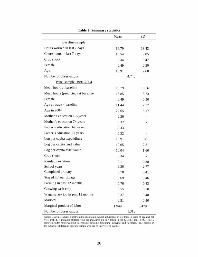
interview from the baseline rounds. By 2004, they were almost 23 years old (Table 1).

7

III.2 Descriptive statistics

Our definition of child labor is the total hours spent working in economic activities and

chores in the previous week (including fetching water and firewood, preparing meals, and

cleaning the house). Economic activities for children consist predominately of farming, including

tending crops in the field, processing crops, and tending livestock. We include chores as well as

economic activities because the concept of child labor typically (e.g., in the ILO standard)

encompasses both,4 although we will distinguish between the two to explain differences in our

results for boys and girls. Children in the sample work on average 17 hours per week, of which

10 are spent on chores (Table 1). Girls spend on average 2.5 hours more than boys working on

household chores; this difference is more pronounced among older girls. More than 90% of

children have worked at least one hour in one of the baseline waves.

We use two instrumental variables: household crop shocks and rainfall shocks.

Household crop shocks are measured as the proportion of crop accidentally lost to pests and fire

during the baseline interview period. Rainfall was measured at 21 weather stations from 1980

onward. For each household, we use rainfall data from the nearest weather station. We construct

the rainfall shock as the deviation of the total rainfall in the short and long rainy seasons

preceding the interview from its 25-year average, scaled by its standard deviation. Table 1 shows

that the average proportion of crop loss is 0.34. The mean of the rainfall shock is -0.11 (i.e., one

4It should also be mentioned that the concept of child labor does not necessarily refer to simply any work done by a

child, but, rather, work that stunts or limits the child’s development or puts the child at risk. However, in survey data

it is difficult to isolate the portion of time spent working on the farm that qualifies under this nuanced definition.

8

tenth of a standard deviation less rain than the weather-station specific norm).5 We discuss the

plausibility of these instruments in Section IV.2 below.

Our education outcome variables are years of schooling and an indicator variable for

having completed seven or more years of education (primary level). Individuals in the sample

have an average of 6.4 years of schooling and 78 percent have completed primary school. We

measure labor market outcomes with a range of variables, including whether the individual earns

a salary or is farming and among those farming whether the individual is growing cash crops. As

the economy in the Kagera region is based mainly on extensive farming, whether the individual

earns a salary or is involved in cash cropping (mainly tobacco and coffee, rather than subsistence

farming) are important indicators of success. We also examine the probability of migrating from

the village6 and the (imputed) marginal productivity of labor in agriculture.

7 The literature has

suggested that plot-specific experience could be an important element of the rural economy

(Rosenzweig and Wolpin, 1985). It is possible that child labor contributes to plot-specific

experience, in which case we would see child labor associated with an increased likelihood of

farming, lower individual mobility, or higher labor productivity.

Finally, we explore whether child labor significantly affects marital status. This is

particularly interesting for our sample of girls, who tend to work more hours than boys,

especially on household chores.8 Since marriage is universal in Tanzania, we are examining the

influence of child labor on the likelihood of earlier marriage. Age at marriage has been shown to

5 By construction, the rainfall deviation variable is mean zero and has a standard deviation of one over the entire

sample period, though not necessarily within sub-periods. 6 While, in wave 5, 70 percent of re-interviewed individuals in the sample were still living in the same or in

neighboring villages, mobility is associated with significantly higher income gains for panel respondents (Beegle,

De Weerdt, and Dercon, 2006b). 7 The marginal productivity of labor is imputed by estimating an agricultural production function. The value of total

agricultural output is regressed on all inputs – including labor and implements – that are used in production. The

procedure is based on Jacoby (1993). 8 For example, girls between 10 and 15 work 22 hours per week (15 of which are spent on household chores), as

opposed to 18 hours for boys (11 of which are spent on household chores).

9

be associated with worse outcomes for women and their children, including increased health

risks as well as potentially “worse” marriage matches.9

IV. Empirical methodology

IV.1 Specification

We are interested in the relationship between outcomes in wave 5 (including education,

occupation, and marital status) and the level of child labor intensity (which we measure through

mean child labor hours in waves 1 to 4). An OLS regression of the form

Yi,t = + Ti,t–10 + Xi,t + i,t, (1)

where Yi,t are outcomes in wave 5, Ti,t–10 is mean child labor hours in waves 1 to 4, and Xi,t are

household and community-level controls, is most probably not suitable for estimating a causal

relationship. The principal concern is omitted variable bias. The child labor decision is likely to

be correlated with both household- and child-level covariates, not all of which will be observable

to the researcher. For example, though we can control for parents’ education we cannot control

for their discount rates. At the child level, we have few covariates other than age and sex, and

thus, for example, cannot control for ability. Reverse causality is less of a concern because the

outcome is measured 10 years after child labor intensity.

We address concerns with the OLS specification using an instrumental variables strategy.

Our instruments, Si,t–10, are indicators of household agricultural shocks and rainfall shocks in

waves 1 to 4. Thus our basic specification is a two-stage least squares procedure of the form:

Ti,t = a + bSi,t + cXi,t + vi,t (2)

9 Younger mothers are more likely to suffer from micronutrient deficiencies and be unaware of the health risks

associated with pregnancy; they are also more likely to have children soon after marriage with increased risk of

maternal and infant mortality (World Bank, 2007). Younger ages at marriage may result in curtailed education for

girls, although it is difficult to ascertain the causality. In any case, a younger bride may be less able to assert power

and authority in her marriage especially given that women marry men who are on average several years older.

10

Yi,t = + ˆ T i,t 10

+ Xi,t + i,i . (3)

In practice, we also include interactions of one of the instruments (crop shocks) with a range of

baseline characteristics (including age, sex, and land per capita) to increase predictive power in

the first stage.

We impose several restrictions on the sample we examine. Following our previous work,

we consider children between the ages of 7 and 15 in the baseline survey. Note that the

prevalence of work among younger children is low. Likewise, by most definitions, working at

age 16 and above would not be viewed as a particularly serious form of child labor. We also

have information on whether children have ever been to school by wave 4. Tabulation of this

variable shows that only 32% of 7-8 year olds had attended school at some point in time, which

is consistent with the widespread tendency to delay enrollment, while among children age 13 and

above only 12% had never been to school. It is unlikely that these older children who have not

yet enrolled will enroll in the future. At the same time, the data suggest that, in response to a

shock, households are more likely to employ the labor of the older, more productive children.

Because of this, if we include these children in our sample, we would be likely to find a strong

negative correlation between years of schooling and child labor. As a result, our sample includes

all 7-15 year olds who were in school at the relevant wave and those children who had not yet

entered school but were still young enough to have a chance to enroll (7-9 year olds).

IV.2 First-stage results and the plausibility of the instruments

In this section, we discuss whether crop and rainfall shocks plausibly satisfy the

requirements for a valid instrumental variable.

11

Relevance

Both crop shocks and rainfall shocks affect the agricultural production function and as

such could have an effect on the use of child labor. Crop shocks reflect occasions of agricultural

stress or crisis, which are moments when the incremental value of child labor may be particularly

high. Rainfall shocks are somewhat more ambiguous. Plentiful rainfall could be a positive shock

to productivity, and, depending on the agricultural production function, could increase the

marginal productivity of child labor. At the same time, extreme outliers of the rainfall deviation

variable – essentially floods – are also possible, and their impact on the use of child labor is less

clear. As it turns out, we do not observe any floods in the first four waves of the survey.

Our previous work and the estimates presented here confirm that crop shocks are

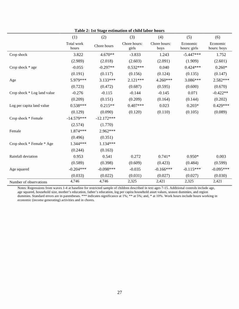
significant predictors of child labor. Table 2 reports estimates from a first-stage regression,

where total child labor hours (column (1)) are regressed on an indicator of crop shocks (and crop

shocks interacted with age, land per capita, a female dummy, and age female), rainfall shocks,

and other regressors (such as region, parental education, log per capita expenditure, and

household size). Column (2) presents the same specification for one of the two components of

total work hours, hours spent in chores; results for the second component of total hours, hours

spent in income-generating work, are not presented, but are available upon request.

The direct effect of a crop shock is a 3.8 hour increase in work and a 4.6 hour increase in

chore hours (with the latter effect significant at the 5 per cent level). Notably the age interaction

is negative for boys and positive for girls for both total work hours and chores: the incremental

work in response to a shock for a 14 year old boy is almost the same as for a 7 year old boy (a

difference of 0.3 hours per week), whereas among girls the older girl would work 4 hours more

in response to a shock than the younger girl. The shock-land interaction is negative (albeit

12

insignificant), implying that the mean level of land holding negates one third of the increased

work hours in response to a shock. The crop shock terms are jointly significant at the one percent

level (with an F-statistic of 9). The rainfall shock has a positive and marginally significant effect

(at the 11 percent level), suggesting that a typical high-rain season is associated with a quarter

hour increase in child labor.

When we split work hours into economic hours (working outside the home in income

generating activities) and chore hours and by boys and girls, we uncover some interesting

differences. The direct effect of a crop shock on time spent on chores is negative for girls and

positive for boys (although neither coefficient is statistically significant), but as can be seen in

Table 2, the age-shock interaction is much larger for girls than boys; the interaction for girls is

statistically significant at the one per cent level and statistically significantly greater than the

point estimate for boys. At a younger age, chore hours increase by a similar amount for boys and

girls in response to a shock, but for older girls the increase in chore hours in response to a shock

is greater than for boys. For example, in response to a shock a 14-year-old girl will work 4

additional chore hours per week compared to a 7 year old, whereas for boys this differential is

negligible. The pattern of variation in economic hours worked among girls is similar to that in

chore hours, with a negative direct effect and a positive age-shock interaction. However, the

magnitudes of the coefficients imply that for younger girls work decreases in response to a

shock, albeit minimally, and for older girls the net effect is close to zero. Instead for boys, the

increase in work hours is approximately 3.5 hours per week for a 7 year old and 5.5 hours per

week for a 15 year old. The rainfall shock variable has a positive and weakly statistically

significant effect on economic hours for girls and chore hours for boys.

13

Overall, this suggests that the incremental effect of the shock is to increase total work

hours for both boys and girls, and to shift girls’ labor hours from economic activities to chores,

while among boys increasing economic activities to a greater degree than chores.

Exogeneity

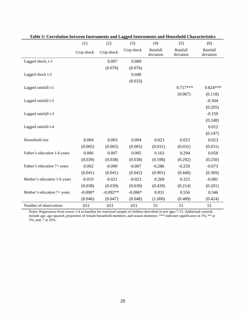
Table 3 examines the plausibility of the exogeneity requirement for our instruments.

Columns (1) to (3) regress crop shocks on lagged crop shocks and household characteristics; the

regressions are at the household level. Column (1) shows that the occurrence of crop shocks is

uncorrelated with most household characteristics, including household size, fathers’ education

and mothers’ primary education. Crop shocks do appear to be negatively correlated with

mothers’ secondary education. It is worth noting less than 2% of the children in the sample have

mothers with more than a primary education. Nonetheless, in our second stage specifications we

include parental education as controls. Columns (2) and (3) show that the occurrence of crop

shocks is uncorrelated with the occurrence of shocks in the previous two survey rounds.

Columns (3) to (6) present analogous results for the rainfall shocks (these regressions are run at

the village level). Rainfall shocks are also uncorrelated with characteristics of the child’s

household, but do appear to be correlated with rainfall in the previous survey wave (column (4)).

In column (6) we see that the correlation in rainfall persists only for one year; rainfall lagged two

years or more does not significantly predict rainfall in the survey year.

Overall, these results suggest that crop and rainfall shocks are plausibly uncorrelated with

respect to household characteristics and over time. The one exception to this – mothers with 7 or

more years of education – can be readily included as a control in the second stage.

14

The Exclusion Restriction

The remaining concern is whether the instruments satisfy the exclusion restriction, i.e. that

they affect education and labor outcomes only through child labor. The relevance of this concern

is supported by an influential strand of literature suggesting that transitory shocks can have long

term consequences for households (see, for example, Ravallion and Lokshin, 2005). We

investigate this concern in a number of ways. First, we examine the reduced form effect of

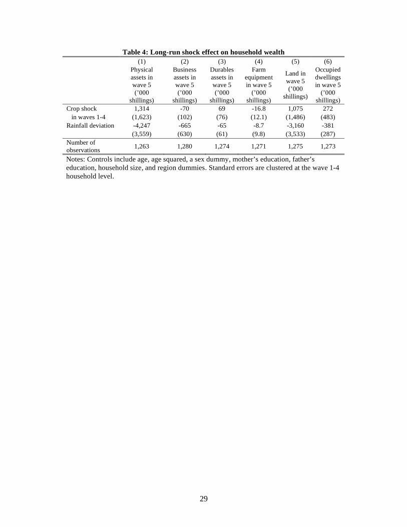
agricultural and rainfall shocks in waves 1 to 4 on a range of outcomes 10 to 13 years later.10

In

particular, we regress wave 5 measures of household wealth, including values of physical and

business assets, durables, farm equipment, land, and occupied dwellings on the average level of

crop and rainfall shocks in waves 1 to 4. The effects are uniformly insignificant (Table 4). These

results suggest, albeit indirectly, that given initial conditions, shocks in waves 1 to 4 did not have

permanent effects on wealth variables in wave 5. In other words, they support the hypothesis that

while shocks account for significant variation in child labor, their effects on other variables are

likely to be short term.

Second, we exploit cross-sectional variation in the size of shocks to test whether our

second stage results are driven only by large shocks or whether we obtain similar results for

smaller shocks. Smaller shocks are a priori less likely to have long-lasting impacts on

households, except through their impact on contemporaneous variables (child labor). We present

these results below (in Section VI.3, along with other robustness checks).

Finally, we use the adults in our data as a comparison group for children. In particular,

using the same specification that we use for children, we test whether labor hours for adults

(those aged 20 and older) in waves 1 to 4 have a significant impact on outcomes in wave 5 when

10

This could be extended by verifying that shocks are not correlated with such causes of attrition in the sample as

mortality and destitution; this is work in progress.

15

instrumented with agricultural shocks. Adults do not, by definition, participate in child labor,

which would imply two possible interpretations for any effect that we find: (1) that the

instruments affect the outcomes directly, through some channel other than child labor (i.e., a

violation of the exclusion restriction) or (2) that the instruments also have an impact on adult

labor which in turn affects outcomes. We present and discuss these results in Section VI.2 below.

V. Results

V.1 Baseline OLS and reduced-form specifications

Prior to discussing our instrumental variables results, we first present the results of OLS

and reduced-form specifications.

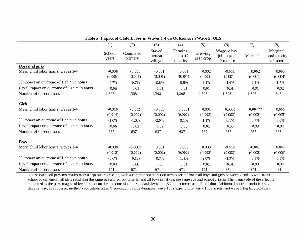
Table 5 presents results from an OLS regression of our outcomes as measured in wave 5

on average child labor over waves 1 to 4. Although the results are not statistically significant and

are also likely to be biased, they are useful baseline estimates for comparison to our instrumental

variables results. Child labor is associated with reduced schooling, which is measured by number

of years of schooling attained and the probability of completing primary education. The negative

association also holds for the probability of staying in or near the village (i.e., staying in the same

village in wave 5 as in the last round of the baseline) and the probability of being a wageworker

in the last 12 months. The results further suggest that child labor is positively correlated with the

probability of being a farmer in the last 12 months, growing cash crops, being married, and labor

productivity. Splitting the sample by gender shows that among girls child labor is associated with

a statistically significant increase in the probability of marriage (which, given the sample

characteristics, typically implies marrying at a younger age). However, because of the potential

16

sources of bias in this specification, as discussed in Section IV.1, we do not interpret these

coefficients causally.

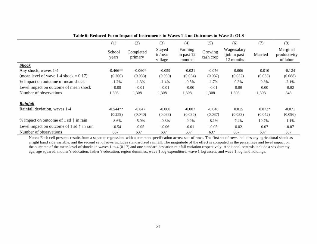
Table 6 presents reduced-form results of regressing our outcomes on the two instrumental

variables. Because the two instruments are reasonably closely correlated, we present results for

each reduced-form result separately11

. The first panel of the table shows that an agricultural

shock has a negative and statistically significant impact on education, measured by completed

years of schooling and by an indicator for completing primary school. The magnitude of this

effect is such that a shock in waves 1 to 4 leads to a one percent loss in education. Agricultural

shocks do not appear to have any significant reduced-form effects on the remaining outcomes.

The rainfall shock has a negative and statistically significant impact on completed

schooling; a one standard deviation increase in rainfall is associated with an 8.6 percent

reduction in completed education. Further, rainfall has a significant impact on the probability of

marriage. A one standard deviation rainfall shock leads to a 10 percent increase in the probability

of marriage. As discussed below, these results are consistent with our IV estimates.

V.2 Instrumental variables estimation

We now discuss our instrumental variables estimates of the impact of child labor hours

on the outcomes of interest. In the first stage, labor hours are predicted from a regression of child

labor hours on shocks and their interactions (Table 2 and equation (3) above).12

11

When both are included simultaneously, results are similar but standard errors are larger, consistent with

multicolinearity 12

Note that as we have on average 2.3 children in the relevant age range per household, the second stage could be

estimated with household fixed effects. However, there is limited variation in education outcomes across children

within a family and a second stage fixed effects specification is unable to estimate the coefficients of interest with

any degree precision.

17

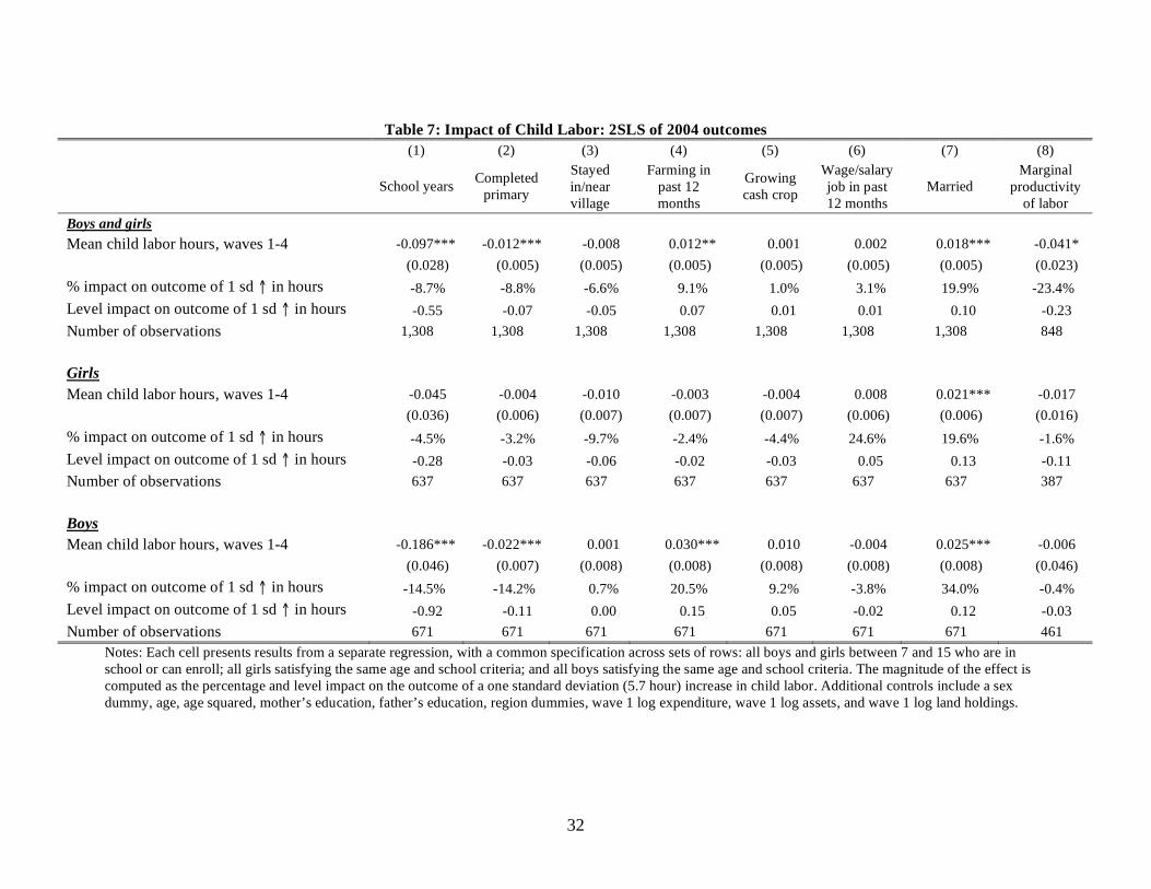
Table 6, columns (1) and (2), show that the 2SLS estimates of the effect of child labor on

education are negative and statistically significant. A one standard deviation increase in child

labor hours (5.7 hours) is associated with a decrease in half a year of schooling and an 8.8

percentage point reduction in the chance of completing primary school. These results are in line

with those obtained for Vietnam by Beegle, Dehejia, and Gatti (2005). Both papers also find that

IV effects are greater than OLS effects.

To the extent that families send the least gifted children to work and skills in the

classroom and in the field are positively correlated, OLS would overestimate the impact of child

labor on schooling, relative to the causal effect (as estimated by IV).13

However, our results

instead lend support to the view that families send their most gifted children to work. To the

extent that children’s work in response to an agricultural shock is critical to the household,

parents may decide to use their most talented children. Another possibility is that there is

significant attenuation bias in the result due to measurement error. This is not implausible: our

measure of child labor (hours worked in the week prior to the survey) is likely to be very noisy.

In column (3), we see that child labor does not appear to be significantly associated with

migration.14

In contrast, column (4) shows that individuals who worked when young are

significantly more likely to be farming in adulthood; a one standard deviation increase in child

labor results in a 9 percentage point increase in the likelihood of farming in adulthood. The

choice between farming cash or subsistence crops is, however, unaffected by working in

childhood (column (5)) 15

Similarly, whether the individual had a wage or salary job in the past

13

This validates one of the key predictions of the model presented in Horowitz and Wang (2004). 14

Results do not change if we include in the sample the children who could not be recontacted between baseline and

wave 5. 15

Note that farming and working for a wage are not mutually exclusive. Of 1,318 people: 180 do neither; 142

working for wage/salary, not farming; 653 farming, not working for wage/salary; 343 both farming and working for

wage/salary.

18

12 months is also not explained by child labor (column (6)). It is interesting to note that child

labor is associated with a significant reduction in the marginal productivity of labor in agriculture

(column (8)). A one standard deviation increase in child labor leads to a 23 percent reduction in

the marginal productivity of labor in agriculture; this effect is significant at the 10 percent level.

Our result on the increased likelihood of farming can be rationalized in the Rosenzweig

and Wolpin (1985) framework in which child labor imparts plot-specific experience that – as

opposed to formal education – is difficult to transfer to other activities. An individual who works

as a child thus benefits from locking himself into farming rather than seeking opportunities in

other sectors or by migrating. Of course, one would have to believe that such plot-specific

knowledge is not being picked up in our estimates of the marginal productivity of labor in

agriculture, which goes down rather than up. Alternatively, our results on farming and the

marginal productivity of labor could simply be viewed as implications of reduced education,

which can both narrow opportunities outside the agricultural sector and – if education and labor

are complementary in the production function – reduce the marginal productivity of labor.

Finally, in column (7), we find that child labor is associated with a significant increase in

the probability of marriage. A one standard deviation (5.7 hour) increase in child labor leads to a

20 percentage point increase in the probability of marriage by wave 5. As noted in the discussion

above, since marriage is almost universal in Kagera, this result suggests that child labor is

associated with earlier marriage.

One of the most striking features of Table 7 is that splitting the results by gender reveals

that the education result is driven by boys. One possible rationalization of this finding is that

parents place a lower priority on the education of girls than boys. Alternatively, chores may be

less harmful to education than agricultural work. As discussed in Section IV.2, Table 2 shows

19

that the incremental effect of crop shocks for girls is an increase in chore hours and a reduction

in economic hours.

The one robustly significant effect of child labor for girls is on the probability of

marriage, which is also positive and significant among boys. There are several possible

interpretations of this. For instance, it is possible that the incremental work induced by our

instrument (namely chores) makes girls more valuable on the marriage market. The marriage

result for boys could similarly reflect the increased value on the marriage market of boys who

have more agricultural experience or could also be the byproduct of reduced educational

opportunities.

VI. Extensions and Robustness Checks

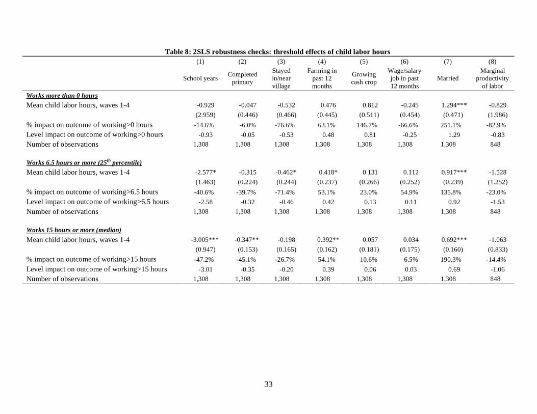
VI.1 Threshold effects in child labor hours

In this section we consider whether the negative effects of child labor estimated in Table 7 are

truly linear or whether there are any threshold effects, i.e., levels of child labor beyond which we

begin to see truly harmful effects but below which child labor is not particularly harmful. Table 8

presents five alternative specifications in which the child labor variable is coded as an indicator

for having worked more than a specified cutoff: 0 hours per week, 6.5 hours per week (the 25th

percentile), 15 hours per week (the median), 24 hours per week (the 75th

percentile), and 35

hours per week (the 90th

percentile).

It is noteworthy that simply working any level of positive hours does not have a

statistically significant impact, other than on marriage. Of course, it must be noted that less than

10 percent of the population do not work, so the effect may not be estimated precisely. When

child labor is coded as working more than 6.5 hours, the four most robust effects from the

20

previous specification (school years, primary schooling, farming, and marriage) now show

statistically significant effects. The magnitude of the school effect is large even at the 25th

percentile of child labor hours: a 40 percent (or 2.5 year) reduction in completed schooling.

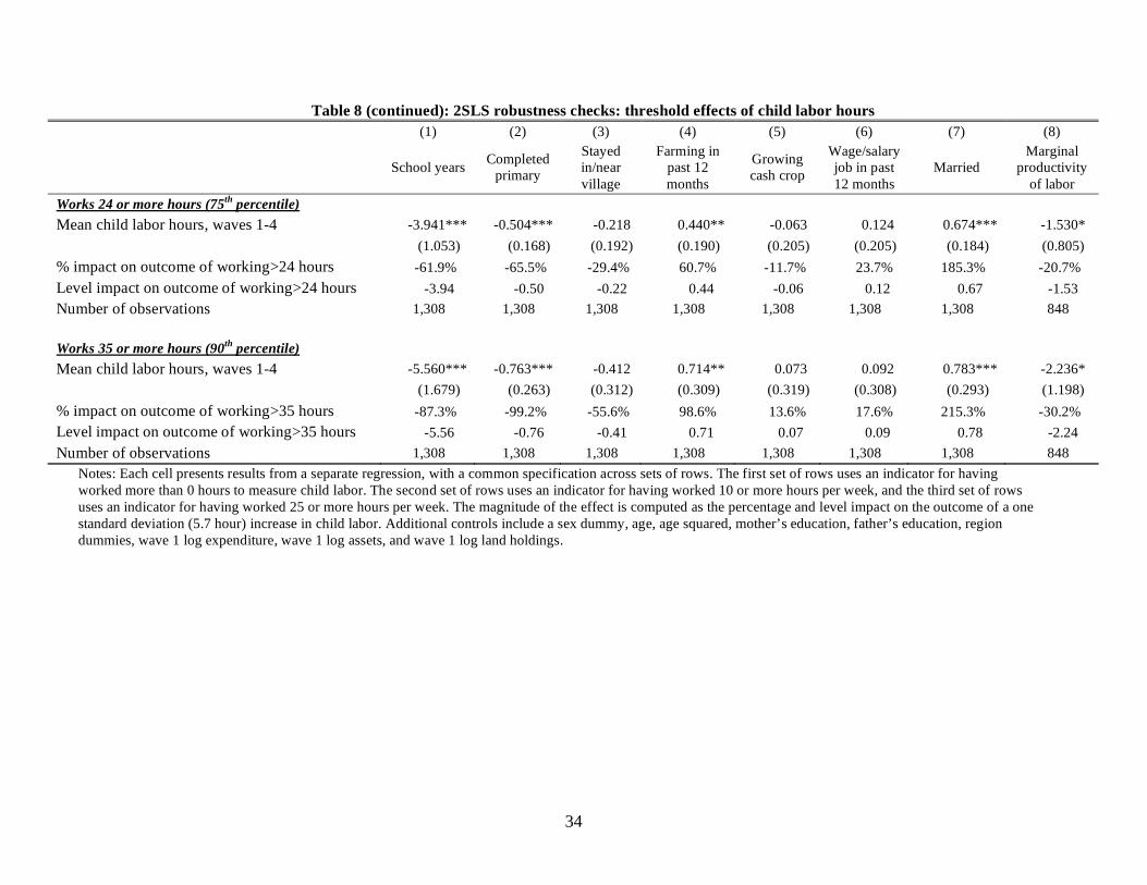
As we increase the threshold for the child labor indicator the magnitudes of the effects

increase. For example, for completed schooling, the effect increases from 3 to 3.9 to 5.6 years of

schooling lost for having worked more than the threshold. For the higher thresholds, the negative

effect on the marginal productivity of labor also begins to kick in as significant.

This exercise suggests that there are significant, negative effects of child labor from even

moderate levels of intensity, but that the effects increase in magnitude with the intensity of child

labor.

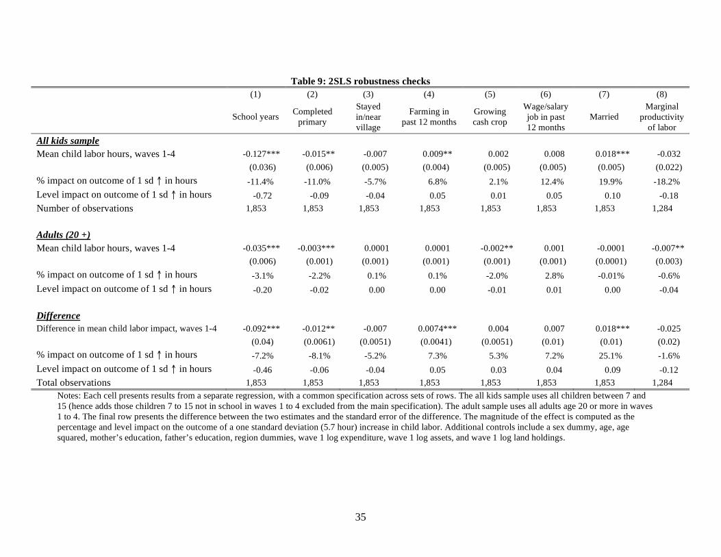
VI.2 Robustness checks: the full sample of children and adults

In this section, we check the sensitivity of our results to the choice of sample. As

discussed in Section IV.1, the regressions in Tables 2-7 are estimated on the sample of 7 to 15

year olds who were either in school as of each wave or who were not in school but still young

enough to start school at some later point (prior to turning 10). This restriction is particularly

important for education outcomes because, while child labor and education are simultaneous

decisions, we are interested in identifying the impact of child labor (rather than, say, delayed

enrollment) on educational attainment. Including children who are unlikely ever to attend school

(i.e. those older than 9 and not at school in wave 4) in the sample would naturally lead us toward

finding a stronger negative impact of child labor on education.

When we run our instrumented regression on the full sample of children between ages 7

and 15 (Table 9, row 1), we find, as expected, larger coefficients for school years and primary

21

school completion. The marriage and farming results are unchanged, but the negative effect on

the marginal productivity of labor is 5 percentage points smaller and no longer statistically

significant. Given that we have added a number of children who were never attending school, the

reduced negative effect on labor productivity suggests that the negative effect we were obtaining

in Table 7 could reflect displaced education.

Next, we turn to the adult sample (individuals aged 20 and older in wave 1) as a

comparison group for the child sample. In particular, we estimate the same two-stage least

squares specification used for children on the adult sample, and also consider the difference

between the estimated effect of work on children and adults. In Table 9, row 2, we see that there

are significant negative effects on school years and the indicator for primary school, although the

magnitudes of these effects are one third to one fifth of the magnitude of the children’s effect.

There are also significant and negative effects for cash crops and the estimated marginal

productivity of labor. There are several possible interpretations. It is possible that there could, in

fact, be a negative effect on schooling, since 71 members of the adult sample are in fact in school

in wave 1. Alternatively, it is possible that there is a direct effect of the instruments being picked

up by instrumented work hours, i.e., that the exclusion restriction fails.

Taking the second interpretation further, if we are willing to assume that the direct, non-

excluded effect of the instruments is the same for adults and children, then we can difference the

two sets of estimates to obtain the effect of child labor; these are presented in Table 9, row 3. As

implied by the children’s and adults’ estimates, there continues to be a significant negative effect

on school years and completion of primary school. These effects are naturally smaller than the

previous estimates, but still substantial in magnitude: a 0.46 year (7.2 percent) loss in schooling

for a one standard deviation increase in child labor hours and a 8 percentage point reduction in

22

the completion of primary school. Likewise, we continue to find positive effects on the

probability of farming and marriage, which are comparable (indeed, greater) in magnitude to our

previous estimates. Because the negative schooling effects for the adult sample could in fact be

due to a reduction in education, we view the estimates in row 3 as being lower bounds for the

child labor effect.

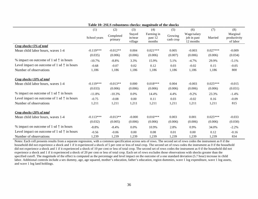
VI.3 Robustness: magnitude of the shock

Finally, we exploit cross-sectional variation in the size of shocks to test whether our second

stage results are driven by large shocks or whether we obtain similar results for smaller shocks.

As discussed in Section IV.2, we are more confident that the exclusion restriction required for a

valid instrumental variable (namely that the instrument affects the outcome only through the

endogenous variable) will be satisfied for small shocks, which are less likely to imply direct long

lasting effects on household outcomes. In Table 10, we re-estimate our results, using three

alternative definitions of the shock (an agricultural shock that results in a loss of respectively at

most 5, 10 and 20 percent of the crop) and excluding those individuals who experienced shocks

larger than the respective thresholds (for example at the 20 percent threshold we exclude 71

individuals from our original sample who experienced a crop loss of greater than 20 percent).

With the exception of labor productivity, we find that our results are similar in magnitude and

significance to our baseline specification in Table 6. This gives us additional confidence in

interpreting our results for education, farming, and marriage causally, and suggests that some

caution is needed in interpreting the negative effect of child labor on adult labor productivity

23

VII. Conclusion and future research

In this paper we investigate the impact of child labor on education and labor market outcomes

using panel data from the Kagera region of Tanzania. Building on our previous work, we use the

occurrence of crop and rainfall shocks as instruments for child labor. In instrumental variables

specifications, we find a negative and significant effect of child labor on school years and the

probability of completing primary school 10 to 13 years later. Moreover, child labor is

significantly positively associated with the probability of being a farmer.

The education results are mainly driven by the sample of boys. For girls we find a

robustly positive effect on the probability of marriage and a somewhat less robust negative effect

on the marginal productivity of labor. In conjunction with our finding that the extra child labor

induced by crop shocks is primarily chores, this suggests the possibility that child labor pushes

girls away from agriculture and toward household activities and marriage. In future work we

intend to use data on bride prices to examine whether child labor in fact increases girls’ value on

the marriage market.

24

References

Akabayashi, H., and Psacharopoulos, George. (1999) “The Trade-off between Child Labor and

Human Capital: A Tanzanian Case.” Journal of Development Studies 35(5): 120-140.

Basu, K. (1999) “Child Labor: Cause, Consequence, and Cure with Remarks on International

Labor Standards.” Journal of Economic Literature 37: 1083-1119.

Beegle, Kathleen, Rajeev Dehejia, and Roberta Gatti (2006) “Child Labor and Agricultural

Shocks.” Journal of Development Economics 81(1): 80-96.

Beegle, Kathleen, Rajeev Dehejia, and Roberta Gatti (2005) “Why Should We Care about Child

Labor? The Education, Labor Market, and Health Consequences of Child Labor.” World Bank

Policy Research Working Paper 3479. CEPR Discussion Paper 4443. NBER Working Paper No.

10980.

Beegle, Kathleen, Joachim De Weerdt, and Stefan Dercon (2006a) “Kagera Health and

Development Survey 2004 Basic Information Document.” World Bank.

Beegle, Kathleen, Joachim De Weerdt, Stefan Dercon (2006b) “Poverty and Wealth Dynamics in

Tanzania: Evidence from a Tracking Survey.” manuscript.

Behrman, Jere R., Alexis Murphy, Agnes Quisumbing, Usha Ramakrishna, and Kathryn Young.

(2006) "What is the Real Impact of Schooling on Age of First Union and Age of First Parenting?

New Evidence from Guatemala.” World Bank Policy Research Working Paper no. 4023.

Bezerra, Márcio Eduardo G., Ana Lúcia Kassouf, Mary Arends-Kuenning. 2007. “The Impact of

Child Labor and School Quality on Academic Achievement in Brazil.” mimeo.

Boozer, Michael, and T. Suri (2001) “Child Labor and Schooling Decisions in Ghana.”

manuscript.

Cavalieri, C. (2002) “The Impact of Child Labor on Educational Performance: An Evaluation of

Brazil.” manuscript.

Emerson, P., and A. Portela Souza (2006) “Is Child Labor Harmful? The Impact of Working

Earlier in Life on Adult Earnings.” manuscript.

Heady, C. (2003) “The Effect of Child Labor on Learning Achievement.” World Development,

31: 385–398.

Horowitz, Andrew, and Jian Wang (2004) “Favorite Son? Specialized Child Laborers and

Students in Poor LDC Households.” Journal of Development Economics 73: 631-642.

International Labour Organization (2003) Investing in Every Child: An Economic Study of the

Costs and Benefits of Eliminating Child Labour. Geneva: International Labour Office.

25

International Labour Organization (2002). A Future Without Child Labour. Geneva: International

Labour Office.

Jacoby, H. (1993). “Shadow Wages and Peasant Family Labor Supply: An Econometric

Application to the Peruvian Sierra,” Review of Economic Studies, 60(4): 903-921

Krutikova, Sofya (2006) “Impact of Child Labor on Education Attainment in Adulthood:

Evidence from Rural Tanzania.” manuscript.

Morduch, Jonathan (1995) “Income Smoothing and Consumption Smoothing.” Journal of

Economic Perspectives 9 (3): 103-14.

O’Donnell O., F. Rosati, and E. Van Doorsaler (2005) “Health Effects of Child Work: Evidence

from Rural Vietnam.”Journal of Population Economics 18(3): 437-467.

Patrinos, H. A., and G. Psacharopoulos (1995) “Educational Performance and Child Labor in

Paraguay.” International Journal of Educational Development 15: 47–60.

Patrinos, H. A., and G. Psacharopoulos (1997) “Family Size, Schooling and Child Labor in

Peru––An Empirical Analysis.” Journal of Population Economics 10: 387– 405.

Pörtner, Klaus (2006) “Gone with the Wind? Hurricane Risk, Fertility and Education.”

Manuscript.

Ravallion, Martin and Michail Lokshin (2005) “Lasting Local Impacts of an Economywide

Crisis.” World Bank Policy Research Working Paper No. 3506.

Ravallion, M. and Q. Wodon (2000) “Does Child Labour Displace Schooling? Evidence on

Behavioral Responses to an Enrollment Subsidy.” The Economic Journal 110: 158-175.

Ray, R., and G. Lancaster (2003) “Does Child Labour Affect School Attendance and School

Performance? Multi Country Evidence on SIMPOC Data.” manuscript.

Rosenzweig, M. and K. Wolpin (1985) “Specific Experience, Household Structure and

Intergenerational Transfers: Farm Family Land and Labor Arrangements in Developing

Countries.” Quarterly Journal of Economics 100: 961-987.

World Bank (2004) “User’s Guide to the Kagera Health and Development Survey Datasets.”

mimeo.

World Bank. (2007) “World Development Report 2007: Development and the Next Generation.”

World Bank.

26

Table 1: Summary statistics

Mean SD

Baseline sample

Hours worked in last 7 days 16.79 13.42

Chore hours in last 7 days 10.54 9.05

Crop shock 0.34 0.47

Female 0.49 0.50

Age 10.91 2.60

Number of observations 4,746

Panel sample: 1991-2004

Mean hours at baseline 16.79 10.56

Mean hours (predicted) at baseline 16.85 5.73

Female 0.49 0.50

Age at wave 4 baseline 11.44 2.77

Age in 2004 22.65 3.17

Mother’s education 1-6 years 0.36 -

Mother’s education 7+ years 0.32 -

Father’s education 1-6 years 0.43 -

Father’s education 7+ years 0.32 -

Log per capita expenditure 10.91 0.81

Log per capita land value 10.05 2.21

Log per capita asset value 10.04 1.60

Crop shock 0.34 -

Rainfall deviation -0.11 0.38

School years 6.36 2.77

Completed primary 0.78 0.41

Stayed in/near village 0.69 0.46

Farming in past 12 months 0.76 0.43

Growing cash crop 0.55 0.50

Wage/salary job in past 12 months 0.37 0.48

Married 0.51 0.50

Marginal product of labor 1,949 3,479

Number of observations 1,313

Notes: Baseline sample is restricted to children in school at baseline or less than 10 years of age and not

yet enrolled. It includes children who are measured up to 4 times in the baseline panel (1991-1994).

Hours includes hours working in economic (income generating) activities and in chores. Panel sample is

the subset of children in baseline sample who are re-interviewed in 2004.

27

Table 2: 1st Stage estimation of child labor hours

(1) (2) (3) (4) (5) (6)

Total work

hours Chore hours

Chore hours:

girls

Chore hours:

boys

Economic

hours: girls

Economic

hours: boys

Crop shock 3.822 4.670** -3.833 1.243 -5.447*** 1.752

(2.989) (2.018) (2.603) (2.091) (1.909) (2.601)

Crop shock * age -0.055 -0.297** 0.532*** 0.040 0.424*** 0.260*

(0.191) (0.117) (0.156) (0.124) (0.135) (0.147)

Age 5.979*** 3.133*** 2.121*** 4.260*** 3.086*** 2.582***

(0.723) (0.472) (0.687) (0.595) (0.600) (0.670)

Crop shock * Log land value -0.276 -0.115 -0.144 -0.145 0.071 -0.422**

(0.209) (0.151) (0.209) (0.164) (0.144) (0.202)

Log per capita land value 0.538*** 0.215** 0.407*** 0.023 0.203* 0.429***

(0.129) (0.090) (0.120) (0.110) (0.105) (0.089)

Crop shock * Female -14.579*** -12.172***

(2.574) (1.770)

Female 1.874*** 2.962***

(0.496) (0.351)

Crop shock * Female * Age 1.344*** 1.134***

(0.244) (0.163)

Rainfall deviation 0.953 0.541 0.272 0.741* 0.950* 0.003

(0.589) (0.398) (0.609) (0.423) (0.484) (0.599)

Age squared -0.204*** -0.098*** -0.035 -0.166*** -0.115*** -0.095***

(0.033) (0.022) (0.031) (0.027) (0.027) (0.030)

Number of observations 4,746 4,746 2,325 2,421 2,325 2,421

Notes: Regressions from waves 1-4 at baseline for restricted sample of children described in text ages 7-15. Additional controls include age,

age squared, household size, mother’s education, father’s education, log per capita household asset values, season dummies, and region

dummies. Standard errors are in parentheses. *** indicates significance at 1%; ** at 5%; and, * at 10%. Work hours include hours working in

economic (income generating) activities and in chores.

28

Table 3: Correlation between Instruments and Lagged Instruments and Household Characteristics

(1) (2) (3) (4) (5) (6)

Crop shock Crop shock Crop shock Rainfall

deviation

Rainfall

deviation

Rainfall

deviation

Lagged shock, t-1 0.097 0.089

(0.076) (0.076)

Lagged shock t-2 0.040

(0.033)

Lagged rainfall t-1 0.717*** 0.824***

(0.067) (0.118)

Lagged rainfall t-2 -0.304

(0.205)

Lagged rainfall t-3 -0.159

(0.248)

Lagged rainfall t-4 0.012

(0.147)

Household size 0.004 0.003 0.004 0.023 0.023 0.023

(0.005) (0.005) (0.005) (0.031) (0.031) (0.031)

Father’s education 1-6 years 0.006 0.007 0.005 0.163 0.294 0.058

(0.039) (0.038) (0.038) (0.598) (0.292) (0.250)

Father’s education 7+ years 0.002 -0.000 -0.007 -0.286 -0.259 -0.073

(0.041) (0.041) (0.042) (0.901) (0.440) (0.369)

Mother’s education 1-6 years -0.019 -0.021 -0.023 0.269 0.325 -0.081

(0.038) (0.039) (0.039) (0.439) (0.214) (0.201)

Mother’s education 7+ years -0.090* -0.092** -0.086* 0.831 0.556 0.346

(0.046) (0.047) (0.048) (1.000) (0.489) (0.424)

Number of observations 651 651 651 51 51 51

Notes: Regressions from waves 1-4 at baseline for restricted sample of children described in text ages 7-15. Additional controls

include age, age squared, proportion of female household members, and season dummies. *** indicates significance at 1%; ** at

5%; and, * at 10%.

29

Table 4: Long-run shock effect on household wealth

(1) (2) (3) (4) (5) (6)

Physical

assets in

wave 5

(’000

shillings)

Business

assets in

wave 5

(’000

shillings)

Durables

assets in

wave 5

(’000

shillings)

Farm

equipment

in wave 5

(’000

shillings)

Land in

wave 5

(’000

shillings)

Occupied

dwellings

in wave 5

(’000

shillings)

Crop shock 1,314 -70 69 -16.8 1,075 272

in waves 1-4 (1,623) (102) (76) (12.1) (1,486) (483)

Rainfall deviation

-4,247 -665 -65 -8.7 -3,160 -381

(3,559) (630) (61) (9.8) (3,533) (287)

Number of

observations 1,263 1,280 1,274 1,271 1,275 1,273

Notes: Controls include age, age squared, a sex dummy, mother’s education, father’s

education, household size, and region dummies. Standard errors are clustered at the wave 1-4

household level.

30

Table 5: Impact of Child Labor in Waves 1-4 on Outcomes in Wave 5: OLS

(1) (2) (3) (4) (5) (6) (7) (8)

School

years

Completed

primary

Stayed

in/near

village

Farming

in past 12

months

Growing

cash crop

Wage/salary

job in past

12 months

Married

Marginal

productivity

of labor

Boys and girls

Mean child labor hours, waves 1-4 -0.008 -0.001 -0.001 0.001 0.002 -0.001 0.002 0.003

(0.009) (0.001) (0.001) (0.001) (0.001) (0.001) (0.001) (0.004)

% impact on outcome of 1 sd in hours -0.7% -0.7% -0.8% 0.8% 2.1% -1.6% 2.2% 1.7%

Level impact on outcome of 1 sd in hours -0.05 -0.01 -0.01 0.01 0.01 -0.01 0.01 0.02

Number of observations 1,308 1,308 1,308 1,308 1,308 1,308 1,308 848

Girls

Mean child labor hours, waves 1-4 -0.010 -0.002 -0.003 0.0001 0.001 0.0001 0.004** 0.006

(0.014) (0.002) (0.002) (0.002) (0.002) (0.002) (0.002) (0.005)

% impact on outcome of 1 sd in hours -1.0% -1.6% -2.9% 0.1% 1.1% 0.1% 3.7% 0.6%

Level impact on outcome of 1 sd in hours -0.06 -0.01 -0.02 0.00 0.01 0.00 0.03 0.04

Number of observations 637 637 637 637 637 637 637 387

Boys

Mean child labor hours, waves 1-4 -0.008 -0.0001 0.001 0.002 0.003 -0.002 -0.001 0.008

(0.012) (0.002) (0.002) (0.002) (0.002) (0.002) (0.002) (0.006)

% impact on outcome of 1 sd in hours -0.6% 0.1% 0.7% 1.4% 2.8% -1.9% 0.1% 0.5%

Level impact on outcome of 1 sd in hours -0.04 0.00 0.00 0.01 0.01 -0.01 0.00 0.04


Notes: Each cell presents results from a separate regression, with a common specification across sets of rows: all boys and girls between 7 and 15 who are in

school or can enroll; all girls satisfying the same age and school criteria; and all boys satisfying the same age and school criteria. The magnitude of the effect is

computed as the percentage and level impact on the outcome of a one standard deviation (5.7 hour) increase in child labor. Additional controls include a sex

dummy, age, age squared, mother’s education, father’s education, region dummies, wave 1 log expenditure, wave 1 log assets, and wave 1 log land holdings.

31

Table 6: Reduced-Form Impact of Instruments in Waves 1-4 on Outcomes in Wave 5: OLS

Notes: Each cell presents results from a separate regression, with a common specification across sets of rows. The first set of rows includes any agricultural shock as

a right hand side variable, and the second set of rows includes standardized rainfall. The magnitude of the effect is computed as the percentage and level impact on

the outcome of the mean level of shocks in waves 1 to 4 (0.17) and one standard deviation rainfall variation respectively. Additional controls include a sex dummy,

age, age squared, mother’s education, father’s education, region dummies, wave 1 log expenditure, wave 1 log assets, and wave 1 log land holdings.

(1) (2) (3) (4) (5) (6) (7) (8)

School

years

Completed

primary

Stayed

in/near

village

Farming

in past 12

months

Growing

cash crop

Wage/salary

job in past

12 months

Married

Marginal

productivity

of labor

Shock

Any shock, waves 1-4 -0.466** -0.060* -0.059 -0.021 -0.056 0.006 0.010 -0.124

(mean level of wave 1-4 shock = 0.17) (0.206) (0.033) (0.039) (0.034) (0.037) (0.032) (0.035) (0.088)

% impact on outcome of mean shock -1.2% -1.3% -1.4% -0.5% -1.7% 0.3% 0.3% -2.1%

Level impact on outcome of mean shock -0.08 -0.01 -0.01 0.00 -0.01 0.00 0.00 -0.02


Rainfall

Rainfall deviation, waves 1-4 -0.544** -0.047 -0.060 -0.007 -0.046 0.015 0.072* -0.071

(0.259) (0.040) (0.038) (0.036) (0.037) (0.033) (0.042) (0.096)

% impact on outcome of 1 sd in rain -8.6% -5.9% -9.3% -0.9% -8.1% 7.4% 10.7% -1.1%

Level impact on outcome of 1 sd in rain -0.54 -0.05 -0.06 -0.01 -0.05 0.02 0.07 -0.07


32

Table 7: Impact of Child Labor: 2SLS of 2004 outcomes

(1) (2) (3) (4) (5) (6) (7) (8)

School years Completed

primary

Stayed

in/near

village

Farming in

past 12

months

Growing

cash crop

Wage/salary

job in past

12 months

Married

Marginal

productivity

of labor

Boys and girls

Mean child labor hours, waves 1-4 -0.097*** -0.012*** -0.008 0.012** 0.001 0.002 0.018*** -0.041*

(0.028) (0.005) (0.005) (0.005) (0.005) (0.005) (0.005) (0.023)

% impact on outcome of 1 sd in hours -8.7% -8.8% -6.6% 9.1% 1.0% 3.1% 19.9% -23.4%

Level impact on outcome of 1 sd in hours -0.55 -0.07 -0.05 0.07 0.01 0.01 0.10 -0.23


Girls

Mean child labor hours, waves 1-4 -0.045 -0.004 -0.010 -0.003 -0.004 0.008 0.021*** -0.017

(0.036) (0.006) (0.007) (0.007) (0.007) (0.006) (0.006) (0.016)

% impact on outcome of 1 sd in hours -4.5% -3.2% -9.7% -2.4% -4.4% 24.6% 19.6% -1.6%

Level impact on outcome of 1 sd in hours -0.28 -0.03 -0.06 -0.02 -0.03 0.05 0.13 -0.11


Boys

Mean child labor hours, waves 1-4 -0.186*** -0.022*** 0.001 0.030*** 0.010 -0.004 0.025*** -0.006

(0.046) (0.007) (0.008) (0.008) (0.008) (0.008) (0.008) (0.046)

% impact on outcome of 1 sd in hours -14.5% -14.2% 0.7% 20.5% 9.2% -3.8% 34.0% -0.4%

Level impact on outcome of 1 sd in hours -0.92 -0.11 0.00 0.15 0.05 -0.02 0.12 -0.03


Notes: Each cell presents results from a separate regression, with a common specification across sets of rows: all boys and girls between 7 and 15 who are in

school or can enroll; all girls satisfying the same age and school criteria; and all boys satisfying the same age and school criteria. The magnitude of the effect is

computed as the percentage and level impact on the outcome of a one standard deviation (5.7 hour) increase in child labor. Additional controls include a sex

dummy, age, age squared, mother’s education, father’s education, region dummies, wave 1 log expenditure, wave 1 log assets, and wave 1 log land holdings.

33

Table 8: 2SLS robustness checks: threshold effects of child labor hours

(1) (2) (3) (4) (5) (6) (7) (8)


primary

Stayed

in/near

village

Farming in

past 12

months

Growing

cash crop

Wage/salary

job in past

12 months

Married

Marginal

productivity

of labor

Works more than 0 hours

Mean child labor hours, waves 1-4 -0.929 -0.047 -0.532 0.476 0.812 -0.245 1.294*** -0.829

(2.959) (0.446) (0.466) (0.445) (0.511) (0.454) (0.471) (1.986)

% impact on outcome of working>0 hours -14.6% -6.0% -76.6% 63.1% 146.7% -66.6% 251.1% -82.9%

Level impact on outcome of working>0 hours -0.93 -0.05 -0.53 0.48 0.81 -0.25 1.29 -0.83


Works 6.5 hours or more (25th

percentile)

Mean child labor hours, waves 1-4 -2.577* -0.315 -0.462* 0.418* 0.131 0.112 0.917*** -1.528

(1.463) (0.224) (0.244) (0.237) (0.266) (0.252) (0.239) (1.252)

% impact on outcome of working>6.5 hours -40.6% -39.7% -71.4% 53.1% 23.0% 54.9% 135.8% -23.0%

Level impact on outcome of working>6.5 hours -2.58 -0.32 -0.46 0.42 0.13 0.11 0.92 -1.53


Works 15 hours or more (median)

Mean child labor hours, waves 1-4 -3.005*** -0.347** -0.198 0.392** 0.057 0.034 0.692*** -1.063

(0.947) (0.153) (0.165) (0.162) (0.181) (0.175) (0.160) (0.833)

% impact on outcome of working>15 hours -47.2% -45.1% -26.7% 54.1% 10.6% 6.5% 190.3% -14.4%

Level impact on outcome of working>15 hours -3.01 -0.35 -0.20 0.39 0.06 0.03 0.69 -1.06


34

Table 8 (continued): 2SLS robustness checks: threshold effects of child labor hours

(1) (2) (3) (4) (5) (6) (7) (8)


primary

Stayed

in/near

village

Farming in

past 12

months

Growing

cash crop

Wage/salary

job in past

12 months

Married

Marginal

productivity

of labor

Works 24 or more hours (75th

percentile)

Mean child labor hours, waves 1-4 -3.941*** -0.504*** -0.218 0.440** -0.063 0.124 0.674*** -1.530*

(1.053) (0.168) (0.192) (0.190) (0.205) (0.205) (0.184) (0.805)

% impact on outcome of working>24 hours -61.9% -65.5% -29.4% 60.7% -11.7% 23.7% 185.3% -20.7%

Level impact on outcome of working>24 hours -3.94 -0.50 -0.22 0.44 -0.06 0.12 0.67 -1.53


Works 35 or more hours (90th

percentile)

Mean child labor hours, waves 1-4 -5.560*** -0.763*** -0.412 0.714** 0.073 0.092 0.783*** -2.236*

(1.679) (0.263) (0.312) (0.309) (0.319) (0.308) (0.293) (1.198)

% impact on outcome of working>35 hours -87.3% -99.2% -55.6% 98.6% 13.6% 17.6% 215.3% -30.2%

Level impact on outcome of working>35 hours -5.56 -0.76 -0.41 0.71 0.07 0.09 0.78 -2.24


Notes: Each cell presents results from a separate regression, with a common specification across sets of rows. The first set of rows uses an indicator for having

worked more than 0 hours to measure child labor. The second set of rows uses an indicator for having worked 10 or more hours per week, and the third set of rows

uses an indicator for having worked 25 or more hours per week. The magnitude of the effect is computed as the percentage and level impact on the outcome of a one

standard deviation (5.7 hour) increase in child labor. Additional controls include a sex dummy, age, age squared, mother’s education, father’s education, region

dummies, wave 1 log expenditure, wave 1 log assets, and wave 1 log land holdings.

35

Table 9: 2SLS robustness checks

(1) (2) (3) (4) (5) (6) (7) (8)


primary

Stayed

in/near

village

Farming in

past 12 months

Growing

cash crop

Wage/salary

job in past

12 months

Married

Marginal

productivity

of labor

All kids sample

Mean child labor hours, waves 1-4 -0.127*** -0.015** -0.007 0.009** 0.002 0.008 0.018*** -0.032

(0.036) (0.006) (0.005) (0.004) (0.005) (0.005) (0.005) (0.022)



Number of observations 1,853 1,853 1,853 1,853 1,853 1,853 1,853 1,284

Adults (20 +)

Mean child labor hours, waves 1-4 -0.035*** -0.003*** 0.0001 0.0001 -0.002** 0.001 -0.0001 -0.007**

(0.006) (0.001) (0.001) (0.001) (0.001) (0.001) (0.0001) (0.003)

% impact on outcome of 1 sd in hours -3.1% -2.2% 0.1% 0.1% -2.0% 2.8% -0.01% -0.6%

Level impact on outcome of 1 sd in hours -0.20 -0.02 0.00 0.00 -0.01 0.01 0.00 -0.04

Difference

Difference in mean child labor impact, waves 1-4 -0.092*** -0.012** -0.007 0.0074*** 0.004 0.007 0.018*** -0.025

(0.04) (0.0061) (0.0051) (0.0041) (0.0051) (0.01) (0.01) (0.02)



Total observations 1,853 1,853 1,853 1,853 1,853 1,853 1,853 1,284

Notes: Each cell presents results from a separate regression, with a common specification across sets of rows. The all kids sample uses all children between 7 and

15 (hence adds those children 7 to 15 not in school in waves 1 to 4 excluded from the main specification). The adult sample uses all adults age 20 or more in waves

1 to 4. The final row presents the difference between the two estimates and the standard error of the difference. The magnitude of the effect is computed as the

percentage and level impact on the outcome of a one standard deviation (5.7 hour) increase in child labor. Additional controls include a sex dummy, age, age

squared, mother’s education, father’s education, region dummies, wave 1 log expenditure, wave 1 log assets, and wave 1 log land holdings.

36

Table 10: 2SLS robustness checks: magnitude of the shocks

(1) (2) (3) (4) (5) (6) (7) (8)


primary

Stayed

in/near

village

Farming in

past 12

months

Growing

cash crop

Wage/salary

job in past

12 months

Married

Marginal

productivity

of labor

Crop shocks<5% of total

Mean child labor hours, waves 1-4 -0.119*** -0.012** 0.004 0.021*** 0.005 -0.003 0.027*** -0.009

(0.035) (0.006) (0.006) (0.006) (0.007) (0.006) (0.006) (0.034)





Mean child labor hours, waves 1-4 -0.119*** -0.013** 0.000 0.018*** 0.004 -0.003 0.025*** -0.015

(0.033) (0.006) (0.006) (0.006) (0.006) (0.006) (0.006) (0.031)





Mean child labor hours, waves 1-4 -0.113*** -0.013** -0.000 0.016*** 0.003 0.001 0.025*** -0.033

(0.032) (0.005) (0.006) (0.006) (0.006) (0.006) (0.006) (0.030)

% impact on outcome of 1 sd in hours -8.8% -8.4% 0.0% 10.9% 2.8% 0.9% 34.0% -2.2%

Level impact on outcome of 1 sd in hours -0.56 -0.06 0.00 0.08 0.01 0.00 0.12 -0.16


Notes: Each cell presents results from a separate regression, with a common specification across sets of rows. The second set of rows codes the instrument as 0 if the

household did not experience a shock and 1 if it experienced a shock of 5 per cent or less of total crop. The second set of rows codes the instrument as 0 if the household

did not experience a shock and 1 if it experienced a shock of 10 per cent or less of total crop. The second set of rows codes the instrument as 0 if the household did not

experience a shock and 1 if it experienced a shock of 20 per cent or less of total crop. Each set of rows excludes those observations with shocks greater than the

specified cutoff. The magnitude of the effect is computed as the percentage and level impact on the outcome of a one standard deviation (5.7 hour) increase in child

labor. Additional controls include a sex dummy, age, age squared, mother’s education, father’s education, region dummies, wave 1 log expenditure, wave 1 log assets,

and wave 1 log land holdings.

Documents

The Consequences of Child Labor: Evidence from ...rdehejia/papers/bdgk.pdfThe Consequences of Child Labor: Evidence from Longitudinal Data ... do find a significant increase in the