THE CONCEPT OF SCALE-CHANGING NETWORK IN THE GLOBAL

Progress In Electromagnetics Research B, Vol. 16, 127–154, 2009

THE CONCEPT OF SCALE-CHANGING NETWORK INTHE GLOBAL ELECTROMAGNETIC SIMULATION OFCOMPLEX STRUCTURES

H. Aubert †

CNRS, LAAS7 avenue du colonel Roche, Toulouse F-31077, France

Abstract—The concept of Scale-Changing Network is reported forthe electromagnetic modeling of complex planar structures composedof a collection of metallic patterns printed on a dielectric surfaceand whose size covers a large range of scale. Examples of suchmulti-scale structures are provided by multi-band frequency-selectivesurfaces, finite-size arrays of non-identical cells and fractal planarobjects. Scale-Changing Networks model the electromagnetic couplingbetween various scale levels in the studied structure and are computedseparately. The cascade of Scale-Changing Networks bridges the gapbetween the smallest and the highest scale levels and allows forminga monolithic (unique) electromagnetic formulation for the globalelectromagnetic simulation of complex planar structures. Derivation ofthese networks is presented and key advantages of the electromagneticapproach are reported.

1. INTRODUCTION

Nowadays global electromagnetic simulators are indispensable foraccurate predictions of the overall electromagnetic performances ofradiofrequency systems. When it involves both large structures (interms of wavelength) and fine details the system or structure is saidcomplex. The higher the number of scale levels the higher complexity.Well-known examples of complex structures are provided by multi-band frequency-selective surfaces, finite-size arrays of non-identicalcells and fractal planar objects. The present paper is focused on theelectromagnetic simulation of a generic multi-scale structure consisting

Corresponding author: H. Aubert ([email protected]).† H. Aubert is also with Universite de Toulouse, UPS, INSA, INP, ISAE, LAAS, ToulouseF-31077, France

128 Aubert

of a collection of metallic patterns printed on a dielectric planar surfaceand whose size covers a large range of scale.

The electromagnetic simulation of multi-scale structures bymeshing-based techniques (e.g., Finite Element Method, FiniteDifference Time-Domain method or Transmission Line Matrix method)requires prohibitive execution time and memory resources. Thenumerical techniques based on spectral discretization (e.g., ModeMatching Technique, Integral Equation-Method developed in thespectral domain) share the same numerical limitations but, in addition,provide densely populated matrices with poor condition numberand suffer from numerical convergence problems when applying tomulti-scale structures. Recently, promising improvements of theMethod of Moments have been proposed for reducing the executiontime and memory storage for large-scale structures — see, e.g.,the impedance matrix localization, the pre-corrected Fast FourierTransform, the Fast Multipole Method and the Generalized SparseMatrix Reduction Technique. However the convergence of numericalresults remains delicate to reach systematically for non-expert users.The Characteristic Basis Method of Moment has been proposedfor solving numerical problems generated by the electromagneticsimulation of multi-scale objects [1, 2] but, the construction ofCharacteristic Basis Functions for expanding the unknown currenton such objects may be very time consuming and may require inpractice large memory storage capabilities. Finally the electromagneticsimulation of multi-scale structures may also be performed by thecombination or hybridization of various numerical techniques, eachtechnique being the most appropriate for each particular scale level.However such coupling between heterogeneous formulations or theinterconnection of various simulation tools is very delicate in practice.

In order to overcome the above-mentioned theoretical andpractical difficulties, an original monolithic (unique) formulation forthe electromagnetic modelling of multi-scale planar structures hasbeen proposed by the author and his collaborators. This newtechnique consists of interconnecting Scale-Changing Networks, eachnetwork models the electromagnetic coupling between adjacent scalelevels. The cascade of Scale Changing Networks allows the globalelectromagnetic simulation of multi-scale structures, from the smallestto the highest scale. Multi-modal sources, called Scale-ChangingSources, are artificially incorporated at all scale levels for the derivationof the network. When the complex surface presents both large regionsand fine details — but no structures at intermediary scale levels-,mono-modal sources are able to model the electromagnetic couplingbetween the disparate scale levels [3–5]. However, for objects involving

Progress In Electromagnetics Research B, Vol. 16, 2009 129

multiple structures whose size covers a large range of scale, mono-modal sources fail to provide accurate numerical results while the Scale-Changing Sources allow the modelling of the scale crossing from thesmallest to the highest scale (the number of modes in these sourcescan be derived from numerical convergence criteria). The globalelectromagnetic simulation of multi-scale structures via the cascadeof Scale Changing Networks has been applied with success to thedesign and electromagnetic simulation of specific planar structuressuch as reconfigurable phase-shifters [6, 7], multi-frequency selectivesurfaces [8], discrete self-similar (pre-fractal) scatterers [9, 10] andpatch antennas [11, 12]. This Scale-Changing technique is a veryfast technique and this makes it a very powerful investigation, designand optimization tool for engineers who design complex circuits (see,e.g., [13–15]). Because of space limitations, the theory behind theproposed technique has never been fully described in our previouspapers, where a particular attention was devoted to specific andattractive applications. The present paper provides the reader detailedtheory on the key concept of Scale-Changing Network. The derivationof the Scale-Changing Network is presented in the framework of ageneric planar multi-scale structure composed of a collection of metallicpatterns printed on a dielectric surface and whose size covers a largerange of scale.

The paper is organized as follows: The concept of Scale-ChangingNetwork is introduced in Section 2. In the framework of Scale-Changing approach passive and active modes are defined and, theScale-Changing Network is derived from the resolution of a specificboundary value problem involving Scale-Changing Sources. TheScale-Changing Sources are defined as intermediary sources that areartificially introduced for the non-redundant computation of the Scale-Changing Networks. The Section 3 is devoted to the Scale-ChangingTechnique, i.e., to the electromagnetic modelling of complex (multi-scale) planar structures via the interconnection of appropriate Scale-Changing Networks. The features of the proposed approach aresummarized. The perspectives foreseen for this work are finallyreported in Section 4.

2. THE SCALE-CHANGING NETWORK

Consider multiple metallic patterns printed on a dielectric surfaceand whose size covers a large range of scale. Suppose that manydecades separate the largest pattern to the smallest one. This complexdiscontinuity plane may be positioned in a waveguide or located infree-space. At both sides of the plane the half-regions are composed of

130 Aubert

multilayered and lossless dielectric media.

2.1. Partitioning of Complex Discontinuity Plane

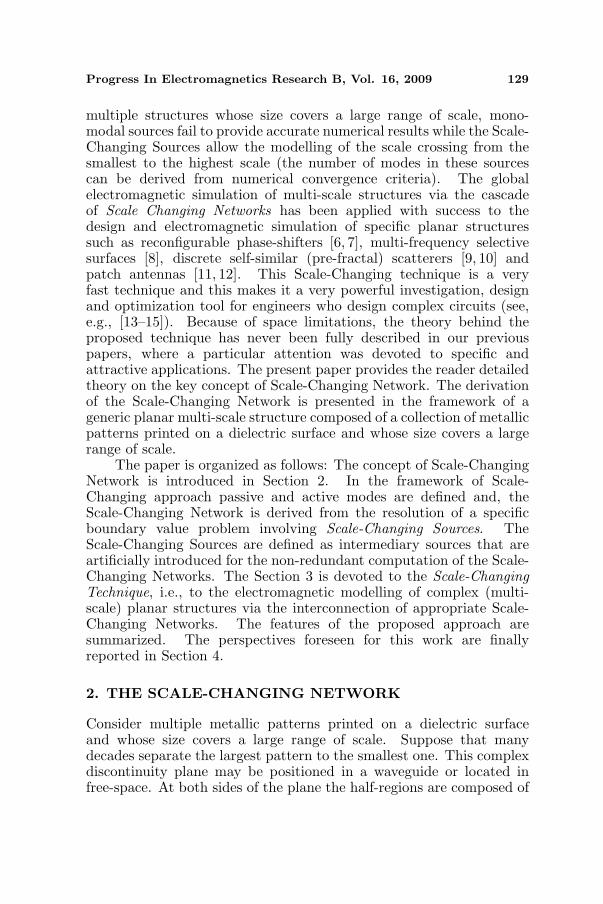
The starting point of the proposed approach consists of the coarsepartitioning of the complex discontinuity plane into large sub-domainsof comparable sizes and arbitrary shape (step 1); in each sub-domain asecond partitioning is performed by introducing smaller sub-domainsof comparable sizes (step 2); Again, in each sub-domain introducedat the previous step a third partitioning is performed by introducingsmaller sub-domains (step 3); and so on, as illustrated on Figure 1.

s = 3

s = 2

s = 1

Scale level s

(a)

(b)

Figure 1. (a) An example of discontinuity plane presenting 3 scale-levels (black is metal and white is dielectric) and (b) the scattered viewof the various sub-domains generated by the partitioning process.

Such hierarchical domain-decomposition allows focusing rapidlyon increasing detail in the discontinuity plane. It is stopped when thefinest dimension — or smallest scale — is reached. To each sub-domainis associated a scale-level: In particular, to the largest sub-domainscorresponds conventionally the scale level s = smax while, the scalelevel s = 1 corresponds to the smallest sub-domains.

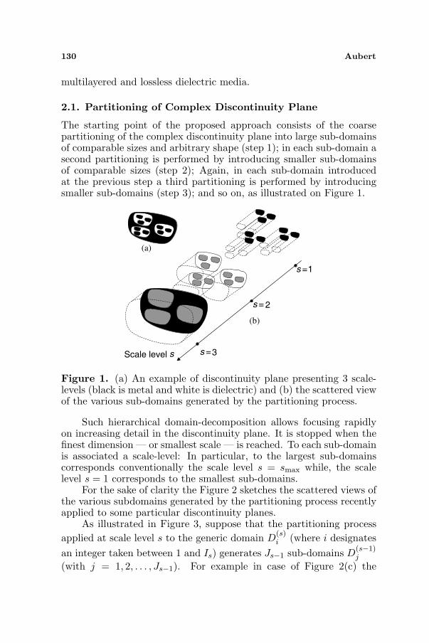
For the sake of clarity the Figure 2 sketches the scattered views ofthe various subdomains generated by the partitioning process recentlyapplied to some particular discontinuity planes.

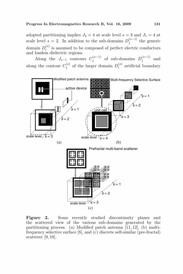
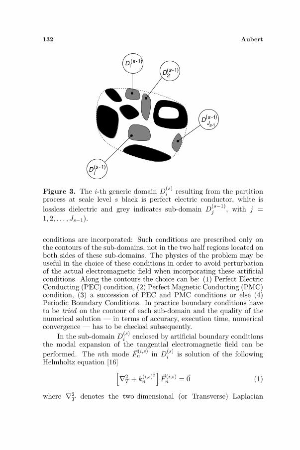
As illustrated in Figure 3, suppose that the partitioning processapplied at scale level s to the generic domain D

(s)i (where i designates

an integer taken between 1 and Is) generates Js−1 sub-domains D(s−1)j

(with j = 1, 2, . . . , Js−1). For example in case of Figure 2(c) the


adopted partitioning implies J2 = 4 at scale level s = 3 and J1 = 4 atscale level s = 2. In addition to the sub-domains D

(s−1)j the generic

domain D(s)i is assumed to be composed of perfect electric conductors

and lossless dielectric regions.Along the Js−1 contours C

(s−1)j of sub-domains D

(s−1)j and

along the contour C(s)j of the larger domain D

(s)i artificial boundary

(a)

scale level s = 3

s = 2

s = 1

active device

Modified patch antenna Multi-frequency Selective Surface

s = 1

s = 2

s = 3

s = 4 scale level

(b)

unit cell

Prefractal multi-band scatterer

scale level s = 3

s = 2

s = 1

(c)

Figure 2. Some recently studied discontinuity planes andthe scattered view of the various sub-domains generated by thepartitioning process. (a) Modified patch antenna [11, 12], (b) multi-frequency selective surface [8], and (c) discrete self-similar (pre-fractal)scatterer [9, 10].

132 Aubert

D)1s(

j-

D)1s(

2-

D)1s(

J 1s

-

-

1D )1s( -

Figure 3. The i-th generic domain D(s)i resulting from the partition

process at scale level s black is perfect electric conductor, white islossless dielectric and grey indicates sub-domain D

(s−1)j , with j =

1, 2, . . . , Js−1).

conditions are incorporated: Such conditions are prescribed only onthe contours of the sub-domains, not in the two half regions located onboth sides of these sub-domains. The physics of the problem may beuseful in the choice of these conditions in order to avoid perturbationof the actual electromagnetic field when incorporating these artificialconditions. Along the contours the choice can be: (1) Perfect ElectricConducting (PEC) condition, (2) Perfect Magnetic Conducting (PMC)condition, (3) a succession of PEC and PMC conditions or else (4)Periodic Boundary Conditions. In practice boundary conditions haveto be tried on the contour of each sub-domain and the quality of thenumerical solution — in terms of accuracy, execution time, numericalconvergence — has to be checked subsequently.

In the sub-domain D(s)i enclosed by artificial boundary conditions

the modal expansion of the tangential electromagnetic field can beperformed. The nth mode ~F

(i,s)n in D

(s)i is solution of the following

Helmholtz equation [16][∇2

T + k(i,s)2

n

]~F (i,s)

n = ~0 (1)

where ∇2T denotes the two-dimensional (or Transverse) Laplacian


operator and k(i,s)n the cut-off wave-number of the nth mode in

D(s)i . Moreover ~F

(i,s)n satisfies the specified (and artificial) boundary

conditions along the contour C(s)i . The discrete set of modes{

~F(i,s)n

}n=1,2,...

in the bounded sub-domain D(s)i is normal that is, for

i = 1, 2, . . . , Is:⟨

~F (i,s)m , ~F

(i,s)

n

⟩=

∫∫

D(s)i

[~F (i,s)

m

]∗·~F (i,s)

n ds = 0 if m 6= n (2)

where[~F

(i,s)m

]∗designates the complex conjugate value of vector ~F

(i,s)m .

In this paper a normalized set of mode{

~F(i,s)n

}n=1,2,...

is used, thus

that is,⟨

~F(i,s)m , ~F

(i,s)

n

⟩= δmn where δmn designates the Kronecker delta

(δmn = 1 if m = n, 0 otherwise).

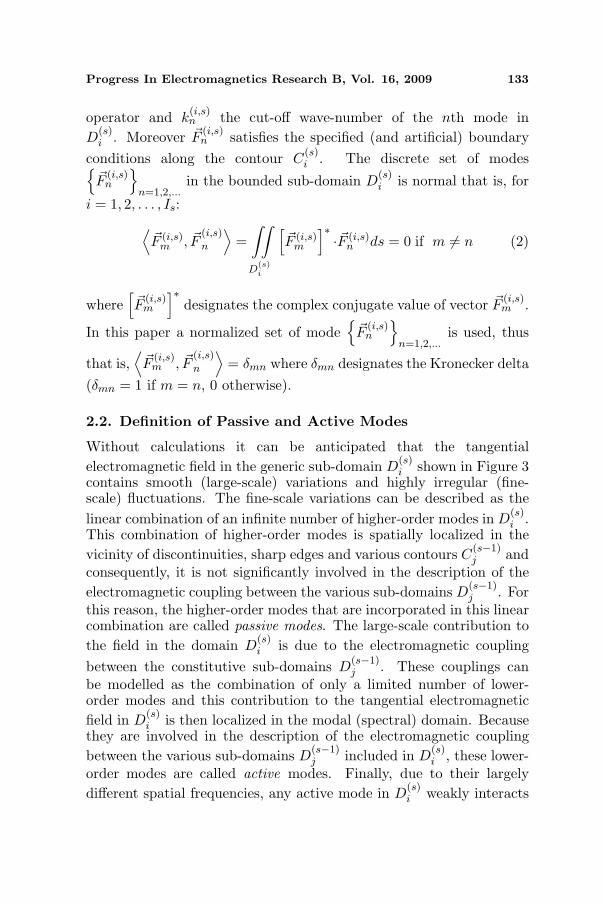
2.2. Definition of Passive and Active Modes

Without calculations it can be anticipated that the tangentialelectromagnetic field in the generic sub-domain D

(s)i shown in Figure 3

contains smooth (large-scale) variations and highly irregular (fine-scale) fluctuations. The fine-scale variations can be described as thelinear combination of an infinite number of higher-order modes in D

(s)i .

This combination of higher-order modes is spatially localized in thevicinity of discontinuities, sharp edges and various contours C

(s−1)j and

consequently, it is not significantly involved in the description of theelectromagnetic coupling between the various sub-domains D

(s−1)j . For

this reason, the higher-order modes that are incorporated in this linearcombination are called passive modes. The large-scale contribution tothe field in the domain D

(s)i is due to the electromagnetic coupling

between the constitutive sub-domains D(s−1)j . These couplings can

be modelled as the combination of only a limited number of lower-order modes and this contribution to the tangential electromagneticfield in D

(s)i is then localized in the modal (spectral) domain. Because

they are involved in the description of the electromagnetic couplingbetween the various sub-domains D

(s−1)j included in D

(s)i , these lower-

order modes are called active modes. Finally, due to their largelydifferent spatial frequencies, any active mode in D

(s)i weakly interacts

134 Aubert

with any passive mode taken in the constitutive sub-domains D(s−1)j .

It follows from these above-mentioned physical considerations that theelectromagnetic coupling between the scale level s and the lower scalelevel s− 1 can be modelled by describing how any active mode in thedomain D

(s)i interacts with the active modes in sub-domains D

(s−1)j .

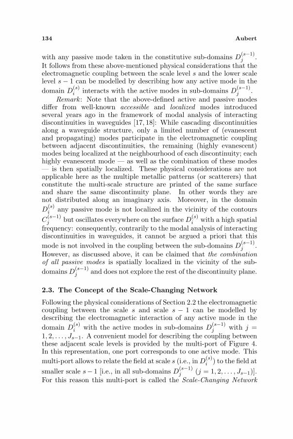
Remark : Note that the above-defined active and passive modesdiffer from well-known accessible and localized modes introducedseveral years ago in the framework of modal analysis of interactingdiscontinuities in waveguides [17, 18]: While cascading discontinuitiesalong a waveguide structure, only a limited number of (evanescentand propagating) modes participate in the electromagnetic couplingbetween adjacent discontinuities, the remaining (highly evanescent)modes being localized at the neighbourhood of each discontinuity; eachhighly evanescent mode — as well as the combination of these modes— is then spatially localized. These physical considerations are notapplicable here as the multiple metallic patterns (or scatterers) thatconstitute the multi-scale structure are printed of the same surfaceand share the same discontinuity plane. In other words they arenot distributed along an imaginary axis. Moreover, in the domainD

(s)i any passive mode is not localized in the vicinity of the contours

C(s−1)j but oscillates everywhere on the surface D

(s)i with a high spatial

frequency: consequently, contrarily to the modal analysis of interactingdiscontinuities in waveguides, it cannot be argued a priori that thismode is not involved in the coupling between the sub-domains D

(s−1)j .

However, as discussed above, it can be claimed that the combinationof all passive modes is spatially localized in the vicinity of the sub-domains D

(s−1)j and does not explore the rest of the discontinuity plane.

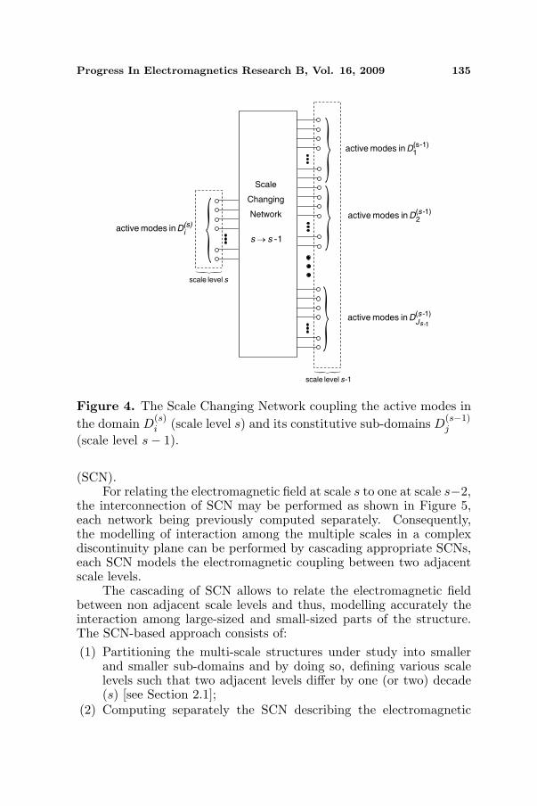
2.3. The Concept of the Scale-Changing Network

Following the physical considerations of Section 2.2 the electromagneticcoupling between the scale s and scale s − 1 can be modelled bydescribing the electromagnetic interaction of any active mode in thedomain D

(s)i with the active modes in sub-domains D

(s−1)j with j =

1, 2, . . . , Js−1. A convenient model for describing the coupling betweenthese adjacent scale levels is provided by the multi-port of Figure 4.In this representation, one port corresponds to one active mode. Thismulti-port allows to relate the field at scale s (i.e., in D

(s)i ) to the field at

smaller scale s− 1 [i.e., in all sub-domains D(s−1)j (j = 1, 2, . . . , Js−1)].

For this reason this multi-port is called the Scale-Changing Network


slevelscale

Dinmodesactive 1)-(s2

Dinmodesactive 1)-(sJ 1-s

Dinmodesactive (s)i

Scale

Changing

Network

1-ss

Dinmodesactive 1)-(s1

1-slevelscale

→

}

}}

}

}

}

Figure 4. The Scale Changing Network coupling the active modes inthe domain D

(s)i (scale level s) and its constitutive sub-domains D

(s−1)j

(scale level s− 1).

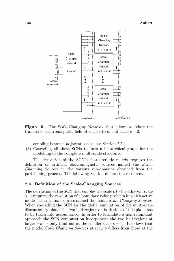
(SCN).For relating the electromagnetic field at scale s to one at scale s−2,

the interconnection of SCN may be performed as shown in Figure 5,each network being previously computed separately. Consequently,the modelling of interaction among the multiple scales in a complexdiscontinuity plane can be performed by cascading appropriate SCNs,each SCN models the electromagnetic coupling between two adjacentscale levels.

The cascading of SCN allows to relate the electromagnetic fieldbetween non adjacent scale levels and thus, modelling accurately theinteraction among large-sized and small-sized parts of the structure.The SCN-based approach consists of:(1) Partitioning the multi-scale structures under study into smaller

and smaller sub-domains and by doing so, defining various scalelevels such that two adjacent levels differ by one (or two) decade(s) [see Section 2.1];

(2) Computing separately the SCN describing the electromagnetic

136 Aubert

Scale-

Changing

Network

2-s1-s

Scale-

Changing

Network

2-s1-s

slevelscale

Scale-

Changing

Network

1-ss

1-slevelscale 2-slevelscale

Scale-

Changing

Network

2-s1-s →

→→

→

}

}}

Figure 5. The Scale-Changing Network that allows to relate thetransverse electromagnetic field at scale s to one at scale s− 2.

coupling between adjacent scales [see Section 2.5];(3) Cascading all these SCNs to form a hierarchical graph for the

modelling of the complete multi-scale structure.

The derivation of the SCN’s characteristic matrix requires thedefinition of artificial electromagnetic sources named the Scale-Changing Sources in the various sub-domains obtained from thepartitioning process. The following Section defines these sources.

2.4. Definition of the Scale-Changing Sources

The derivation of the SCN that couples the scale s to the adjacent scales−1 requires the resolution of a boundary value problem in which activemodes act as actual sources named the modal Scale Changing Sources.When cascading the SCN for the global simulation of the multi-scalediscontinuity plane, the two half regions on both sides of this plane hasto be taken into accountonce. In order to formulate a non redundantapproach the SCN computation incorporates the two half-regions atlarger scale s only (and not at the smaller scale s− 1). It follows thatthe modal Scale Changing Sources at scale s differs from those at the


smaller scale s− 1.

2.4.1. Modal Scale-Changing Sources at the Larger Scale

At both sides of the generic sub-domain D(s)i shown in Figure 3 the

half-regions are composed of multilayered and lossless dielectric media.Throughout the paper these half-regions are denoted by the capitalletters A and B, respectively. For α = A,B let D

(i,s)α be the plane

located in the half-region α and positioned infinitely close to thedomain D

(s)i ; in addition let ~nα be the unit vector normal to D

(i,s)α and

oriented toward the half-region α; and finally, let ~E(i,s)α and ~H

(i,s)α be

respectively the tangential electric and magnetic fields on the domainD

(i,s)α . The set

{~F

(i,s)n

}n=1,2,...

of modes introduced in Section 2.1 is

now used for the expansion of the tangential electromagnetic fieldsinside D

(i,s)A and D

(i,s)B , that is:

~E(i,s)α =

∞∑n=1

V(i,s,α)n

~F(i,s)n

~J(i,s)α = ~H

(i,s)α × ~nα =

∞∑n=1

I(i,s,α)n

~F(i,s)n

with α = A, B (3)

where V(i,s,α)n and I

(i,s,α)n denote respectively, the voltage and current

amplitudes of the n-th mode in D(i,s)α . Following the physical

considerations of Section 2.2, the tangential electric field ~E(i,s)α and

the current density ~J(i,s)α = ~H

(i,s)α × ~nα in D

(i,s)α may be written as

follows:

~E(i,s)α = ~E

(i,s)α

∣∣∣large

+ ~E(i,s)α

∣∣∣fine

~J(i,s)α = ~J

(i,s)α

∣∣∣large

+ ~J(i,s)α

∣∣∣fine

(4)

with

~E(i,s)α

∣∣∣large

=N

(i,s)α∑

n=1V

(i,s,α)n

~F(i,s)n and ~E

(i,s)α

∣∣∣fine

=∞∑

n=N(i,s)α +1

V(i,s,α)n

~F(i,s)n

~J(i,s)α

∣∣∣large

=N

(i,s)α∑

n=1I

(i,s,α)n

~F(i,s)n and ~J

(i,s)α

∣∣∣fine

=∞∑

n=N(i,s)α +1

I(i,s,α)n

~F(i,s)n

(5)

where N(i,s)α denotes the number of active (propagating and

evanescent) modes in the waveguide of cross-section D(i,s)α . Since they

138 Aubert

are highly evanescent in the artificial half-waveguide α (with α = A,B),passive modes may be shunted by the purely reactive modal admittanceY

(i,s,α)n viewed by D

(i,s)α . The analytical and generic expression of the

modal admittance Y(i,s,α)n in case of multilayered dielectric structure

located may be found in [19]. Consequently:

I(i,s,α)n ≈ Y (i,s,α)

n V (i,s,α)n for n > N (i,s)

α (6)

From Eqs. (5) and (6) it can be deduced that

~J (i,s)α ≈ J (i,s)

α

∣∣∣large

+∞∑

n=N(i,s)α +1

Y (i,s,α)n V (i,s,α)

n~F (i,s)

n (7)

This expression may be formally written as followed:

~J (i,s)α = ~J (i,s)

α

∣∣∣large

+ Y (i,s)α

~E(i,s)α

with Y (i,s)α =

∞∑

n=N(i,s)α +1

∣∣∣~F (i,s)n

⟩Y (i,s,α)

n

⟨~F (i,s)

n

∣∣∣ (8)

where Y(i,s)α is an admittance operator. Note that only the passive

modes in the half-waveguide α (with α = A,B) are involved in Y(i,s)α .

Following (5) the boundary conditions on the domain D(s)i [that is,

~E(s)i = ~E

(i,s)A = ~E

(i,s)B ] becomes:

∞∑

n=1

V (i,s)n

~F (i,s)n =

∞∑

n=1

V (i,s,A)n

~F (i,s)n =

∞∑

n=1

V (i,s,B)n

~F (i,s)n

⇒ V (i,s)n = V (i,s,A)

n = V (i,s,B)n (9)

where V(i,s)n denotes the voltage amplitude of the nth mode in D

(s)i .

Moreover, following Eq. (8), the current density ~J(s)i = ~J

(i,s)A + ~J

(i,s)B

in D(s)i becomes:

~J(s)i = ~J

(s)i

∣∣∣large

+ Y(s)i

~E(s)i (10)

where

~J(s)i

∣∣∣large

=∑

α=A,B

~J(i,s)α

∣∣∣large

=N

(i,s)A∑

n=1I

(i,s,A)n

~F(i,s)n +

N(i,s)B∑

n=1I

(i,s,B)n

~F(i,s)n

Y(s)i = Y

(i,s)A +Y

(i,s)B =

∑α=A,B

∞∑n=N

(i,s)α +1

∣∣∣~F (i,s)n

⟩Y

(i,s,α)n

⟨~F

(i,s)n

∣∣∣(11)


For the sake of simplification in the theoretical developments thenumber of active modes in domains D

(i,s)A and D

(i,s)B may be taken

identical, that is, N(i,s)A = N

(i,s)B = N (i,s) where N (i,s) refers to

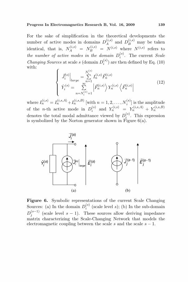
the number of active modes in the domain D(s)i . The current Scale

Changing Sources at scale s (domain D(s)i ) are then defined by Eq. (10)

with:

~J(s)i

∣∣∣large

=N

(s)i∑

n=1I

(i,s)n

~F(i,s)n

Y(s)i =

∞∑n=N

(s)i +1

∣∣∣~F (i,s)n

⟩Y

(i,s)n

⟨~F

(i,s)n

∣∣∣(12)

where I(i,s)n = I

(i,s,A)n +I

(i,s,B)n [with n = 1, 2, . . . , N

(s)i ] is the amplitude

of the n-th active mode in D(s)i and Y

(i,s)n = Y

(i,s,A)n + Y

(i,s,B)n

denotes the total modal admittance viewed by D(s)i . This expression

is symbolized by the Norton generator shown in Figure 6(a).

(a) (b)

)s(i

J

)s(i

Ylarge

(s)

iJ )s(iE

)1s(j

E-)1s(

jJ -

→

→ →→ →

Figure 6. Symbolic representations of the current Scale ChangingSources: (a) In the domain D

(s)i (scale level s); (b) In the sub-domain

D(s−1)j (scale level s − 1). These sources allow deriving impedance

matrix characterizing the Scale-Changing Network that models theelectromagnetic coupling between the scale s and the scale s− 1.

140 Aubert

2.4.2. Modal Scale-Changing Sources at the Smaller Scale

The current Scale-Changing source in the sub-domain D(s−1)j (scale

s − 1) is defined as the linear combination of N(s−1)j active modes as

followed:

~J(s−1)j = ~J

(s−1)j

∣∣∣large

=N

(s−1)j∑

n=1

I(j,s−1)n

~F (j,s−1)n (13)

where I(j,s−1)n

~F(j,s−1)n denotes the current density of the n-th active

mode in the sub-domain D(s−1)j . Modelling the coupling between the

scale s and scale s − 1, the contribution ~J(s−1)j

∣∣∣fine

of passive modes

to the total current density ~J(s−1)j in D

(s−1)j does not act as an actual

source. The symbolic representation of the current Scale ChangingSource at scale s−1 is shown in Figure 6(b). At this smaller scale, theadmittance operator that models the half-regions located on both sidesof the discontinuity plane is not taken into consideration unlike at the

D)1s( -

)s(1

Y)s(

D

)s(1

Y)s(

C

C1)s( -

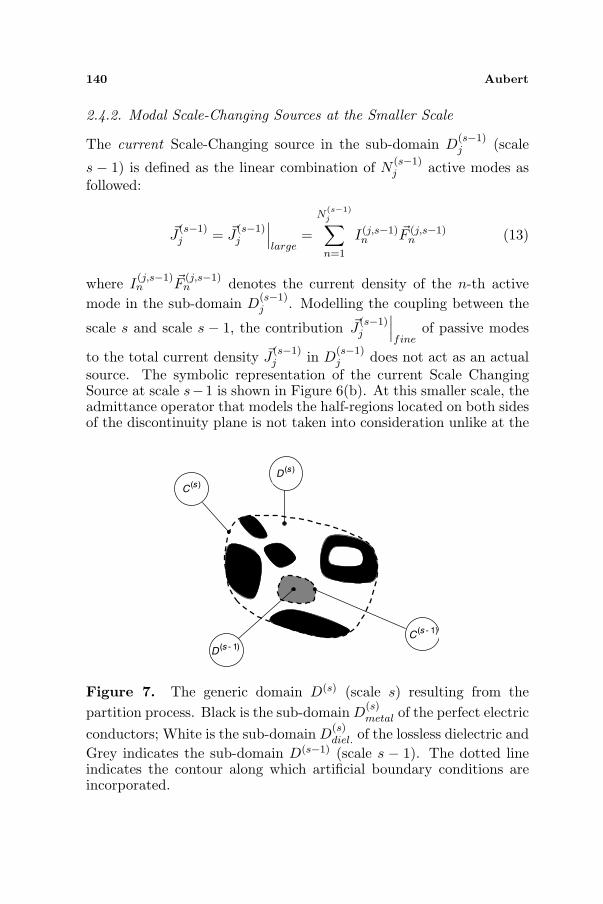
Figure 7. The generic domain D(s) (scale s) resulting from thepartition process. Black is the sub-domain D

(s)metal of the perfect electric

conductors; White is the sub-domain D(s)diel. of the lossless dielectric and

Grey indicates the sub-domain D(s−1) (scale s − 1). The dotted lineindicates the contour along which artificial boundary conditions areincorporated.


higher scale level s: this choice allows eliminating redundancies in thetheoretical formulation when cascading of Scale-Changing Networks.

2.5. Derivation of the Scale-Changing Network

The objective of this section is to derive the SCN that models theelectromagnetic coupling between two adjacent scale levels, that is,the coupling between active modes in the generic domain D

(s)i and its

constitutive sub-domains D(s−1)j (j = 1, 2, . . . , Js−1).

2.5.1. Formulation of the Boundary Value Problem

For the sake of clarity in the theoretical developments, consider thedomain D(s) composed of one sub-domain D(s−1) (see Figure 7).

The domain of perfectly conducting metallic patterns is denotedD

(s)metal while the domain D

(s)diel. designates the lossless dielectric region.

The generalization of this problem to multiple sub-domains D(s−1)j

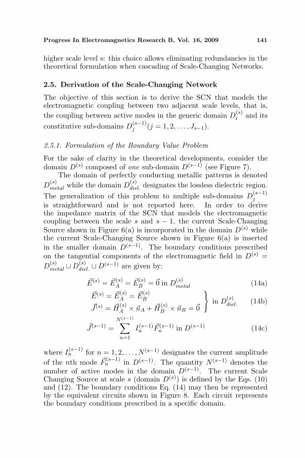
is straightforward and is not reported here. In order to derivethe impedance matrix of the SCN that models the electromagneticcoupling between the scale s and s − 1, the current Scale-ChangingSource shown in Figure 6(a) is incorporated in the domain D(s) whilethe current Scale-Changing Source shown in Figure 6(a) is insertedin the smaller domain D(s−1). The boundary conditions prescribedon the tangential components of the electromagnetic field in D(s) =D

(s)metal ∪D

(s)diel. ∪D(s−1) are given by:

~E(s) = ~E(s)A = ~E

(s)B = ~0 in D

(s)metal (14a)

~E(s) = ~E(s)A = ~E

(s)B

~J (s) = ~H(s)A × ~nA + ~H

(s)B × ~nB = ~0

}in D

(s)diel. (14b)

~J (s−1) =N(s−1)∑

n=1

I(s−1)n

~F (s−1)n in D(s−1) (14c)

where I(s−1)n for n = 1, 2, . . . , N (s−1) designates the current amplitude

of the nth mode ~F(s−1)n in D(s−1). The quantity N (s−1) denotes the

number of active modes in the domain D(s−1). The current ScaleChanging Source at scale s (domain D(s)) is defined by the Eqs. (10)and (12). The boundary conditions Eq. (14) may then be representedby the equivalent circuits shown in Figure 8. Each circuit representsthe boundary conditions prescribed in a specific domain.

142 Aubert

(a) (b) (c)

)s(J

)s(Y )s(

Y)s(

J)1s(

J)s(

J)s(

Y→ → → →

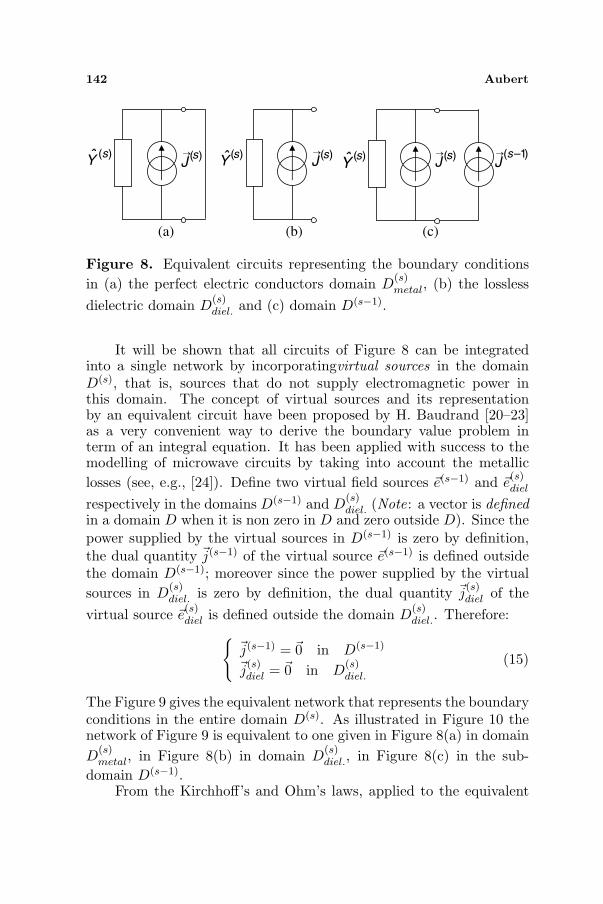
Figure 8. Equivalent circuits representing the boundary conditionsin (a) the perfect electric conductors domain D

(s)metal, (b) the lossless

dielectric domain D(s)diel. and (c) domain D(s−1).

It will be shown that all circuits of Figure 8 can be integratedinto a single network by incorporatingvirtual sources in the domainD(s), that is, sources that do not supply electromagnetic power inthis domain. The concept of virtual sources and its representationby an equivalent circuit have been proposed by H. Baudrand [20–23]as a very convenient way to derive the boundary value problem interm of an integral equation. It has been applied with success to themodelling of microwave circuits by taking into account the metalliclosses (see, e.g., [24]). Define two virtual field sources ~e(s−1) and ~e

(s)diel

respectively in the domains D(s−1) and D(s)diel. (Note: a vector is defined

in a domain D when it is non zero in D and zero outside D). Since thepower supplied by the virtual sources in D(s−1) is zero by definition,the dual quantity ~j(s−1) of the virtual source ~e(s−1) is defined outsidethe domain D(s−1); moreover since the power supplied by the virtualsources in D

(s)diel. is zero by definition, the dual quantity ~j

(s)diel of the

virtual source ~e(s)diel is defined outside the domain D

(s)diel.. Therefore:

{~j(s−1) = ~0 in D(s−1)

~j(s)diel = ~0 in D

(s)diel.

(15)

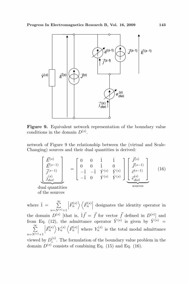
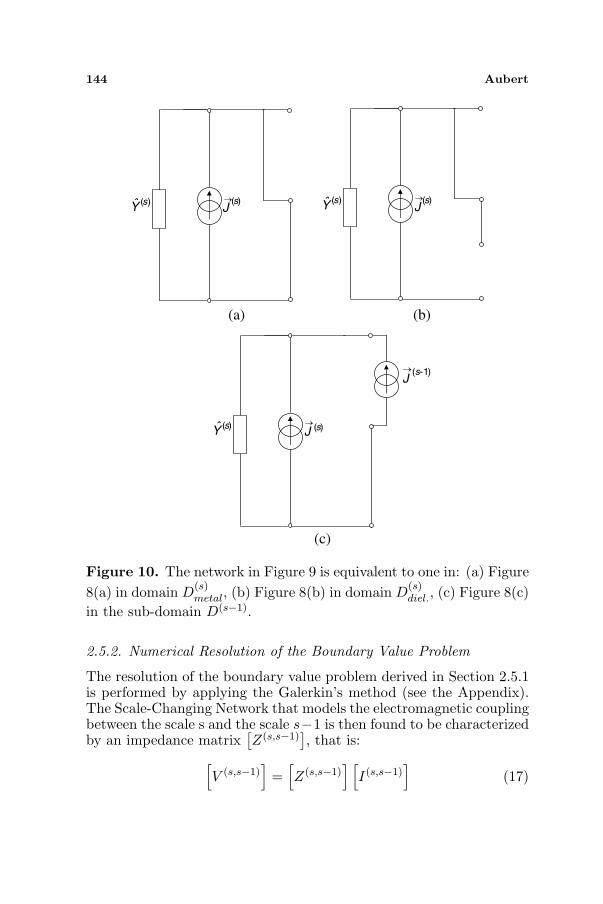
The Figure 9 gives the equivalent network that represents the boundaryconditions in the entire domain D(s). As illustrated in Figure 10 thenetwork of Figure 9 is equivalent to one given in Figure 8(a) in domainD

(s)metal, in Figure 8(b) in domain D

(s)diel., in Figure 8(c) in the sub-

domain D(s−1).From the Kirchhoff’s and Ohm’s laws, applied to the equivalent


)s(J

)s(Y

)s(E

)1s(e - )1s(J

-

)1s(j -

)1s(E

-

)s(.diel

e

)s(.diel

j

→ →→

→

→ →

→

Figure 9. Equivalent network representation of the boundary valueconditions in the domain D(s).

network of Figure 9 the relationship between the (virtual and Scale-Changing) sources and their dual quantities is derived:

~E(s)

~E(s−1)

~j(s−1)

j(s)diel

︸︷︷︸dual quantitiesof the sources

=

0 0 1 10 0 1 0−1 −1 Y (s) Y (s)

−1 0 Y (s) Y (s)

~J (s)

~J (s−1)

~e(s−1)

~e(s)diel

︸︷︷︸sources

(16)

where 1 =∞∑

n=N(s)+1

∣∣∣~F (s)n

⟩ ⟨~F

(s)n

∣∣∣ designates the identity operator in

the domain D(s) [that is, 1~f = ~f for vector ~f defined in D(s)] andfrom Eq. (12), the admittance operator Y (s) is given by Y (s) =

∞∑n=N(s)+1

∣∣∣~F (s)n

⟩Y

(s)n

⟨~F

(s)n

∣∣∣ where Y(s)n is the total modal admittance

viewed by D(s)i . The formulation of the boundary value problem in the

domain D(s) consists of combining Eq. (15) and Eq. (16).

144 Aubert

(a) (b)

)s(J

)s(Y

)s(J

)s(Y

(c)

)s(J

)s(Y

)1s(J

-

→ →

→

→

Figure 10. The network in Figure 9 is equivalent to one in: (a) Figure8(a) in domain D

(s)metal, (b) Figure 8(b) in domain D

(s)diel., (c) Figure 8(c)

in the sub-domain D(s−1).

2.5.2. Numerical Resolution of the Boundary Value Problem

The resolution of the boundary value problem derived in Section 2.5.1is performed by applying the Galerkin’s method (see the Appendix).The Scale-Changing Network that models the electromagnetic couplingbetween the scale s and the scale s−1 is then found to be characterizedby an impedance matrix

[Z(s,s−1)

], that is:

[V (s,s−1)

]=

[Z(s,s−1)

] [I(s,s−1)

](17)


slevelscale

- )1,( ssZ

1-slevelscale

)s(1V

)s(2V

)s(

N)s(V

)1s(1V

-

)1s(2V

-

)1s(

N )1s(V--

)s(1I

)1s(1I

-

)1s(2I

-

)1s(

N)1s(I

--

)s(2I

)s(

N)s(I

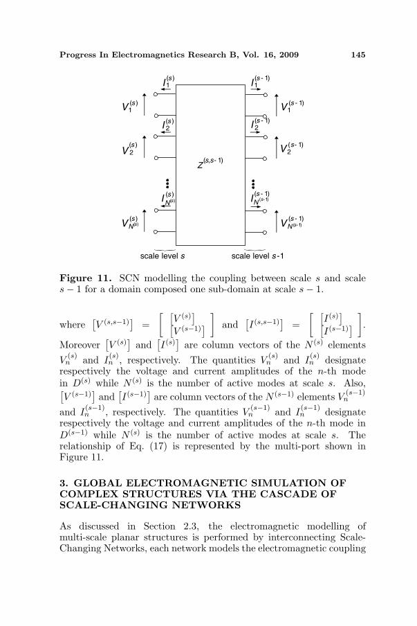
}}Figure 11. SCN modelling the coupling between scale s and scales− 1 for a domain composed one sub-domain at scale s− 1.

where[V (s,s−1)

]=

[ [V (s)

][V (s−1)

]]

and[I(s,s−1)

]=

[ [I(s)

][I(s−1)

]].

Moreover[V (s)

]and

[I(s)

]are column vectors of the N (s) elements

V(s)n and I

(s)n , respectively. The quantities V

(s)n and I

(s)n designate

respectively the voltage and current amplitudes of the n-th modein D(s) while N (s) is the number of active modes at scale s. Also,[V (s−1)

]and

[I(s−1)

]are column vectors of the N (s−1) elements V

(s−1)n

and I(s−1)n , respectively. The quantities V

(s−1)n and I

(s−1)n designate

respectively the voltage and current amplitudes of the n-th mode inD(s−1) while N (s) is the number of active modes at scale s. Therelationship of Eq. (17) is represented by the multi-port shown inFigure 11.

3. GLOBAL ELECTROMAGNETIC SIMULATION OFCOMPLEX STRUCTURES VIA THE CASCADE OFSCALE-CHANGING NETWORKS

As discussed in Section 2.3, the electromagnetic modelling ofmulti-scale planar structures is performed by interconnecting Scale-Changing Networks, each network models the electromagnetic coupling

146 Aubert

between two adjacent scales. The reduction of the electromagneticmodelling of complex structures to the cascade of Scale-ChangingNetworks (SCN) is called the Scale-Changing Technique (SCT). Thismonolithic (unique) approach for the global electromagnetic simulationof complex structures does not require delicate interconnection ofheterogeneous theoretical formulations. Due to the hierarchical-domain decomposition provided by the partitioning process, thecomplex structures are broken down into a finite number of scalelevels; next all the SCN that relate the electromagnetic field at adjacentscales are separately computed and, the hierarchical interconnection ofthe SCN is finally performed for global electromagnetic simulation ofcomplex (multi-scale) structures. The scale crossing from the smallestto the arbitrary scale S is performed by shunting the cascade of SCNby the equivalent multi-ports modelling the smallest scale. When thedimensions of a sub-domain are small compared to the wavelength thecorresponding multi-port reduces to one-port classically called surfaceimpedance. However, for reaching the convergence of the numericalresults, the larger the size of the sub-domain the higher the number ofactive and passive modes.

The SCN-based approach avoids the direct computation ofstructure with high aspect ratio and consequently, as far as thenumber of modes in the computation of SCN is not very large, itdoes thus not suffer from the treatment of ill-conditioned matrices andthe lack of proper convergence. Typically, if N orders of magnitude(or decades) separate the largest to the smallest dimensions in thestructure the SCN-based global electromagnetic simulation requiresthe computation of N SCN (or matrices), while tremendous executiontime and memory resources are required by other numerical techniquesfor handling the corresponding aspect ratio of 10N . Moreover, theSCN can be computed separately and consequently, the SCN-basednumerical technique is highly parallelizable.

In the design and optimization processes modifications of thestructure geometry may occur at a given scale S. Contrarily toclassical meshing-based techniques, these modifications do not requirethe recalculation of the overall structure but only the SCN modelingthe electromagnetic coupling between scale S and S − 1 and, betweenS + 1 and S. Such modularity makes the SCN-based approach veryefficient in terms of CPU time and a very powerful analysis, design andoptimization tool for engineers who design complex structures.

When dimensions of domains are large compared to thewavelength high-frequency techniques based on the asymptoticelectromagnetic approaches (e.g., Physical Theory of Diffraction) mustbe preferred to the SCT and low-frequency techniques are also more


efficient than SCT at fine scale. However the SCT seems to be a goodcandidate to provide an efficient and powerful approach for bridgingthe gap between high- and low-frequency techniques, that is, betweenlarge- and small-scale electromagnetic modelling.

Illustration of all the above mentioned features and quantitativeinformation about execution time in some specific cases may be foundin the previous reports [6, 8]. These illustrations cover bounded andun-bounded structures. In particular it has been shown that the SCN-based approach can be advantageously applied to pre-fractal planarstructures, that is, to complex structures presenting scale-invariancesymmetry over a wide scale range. It consists of an alternativetechnique to the renormalization approach proposed by H. Baudrandet al. [26, 27]. The proposed technique reduces in these cases tosimple recurrent relationships and allows a dramatic reduction inthe computational time compared to classical numerical techniques,especially when the complexity — i.e., the number of scale levels — ishigh (see, e.g., [8]).

4. CONCLUSION

A monolithic formulation for the global electromagnetic simulationof multi-scale 2.5D structures has been presented. It consists ofthe cascade of Scale-Changing Networks, each network models theelectromagnetic coupling between adjacent scale levels. By itsvery nature, this formulation is highly parallelizable, which alsodistinguishes it from other techniques that have to be adapted fordistributed processing.

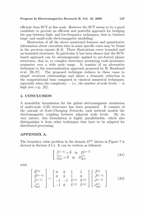
APPENDIX A.

The boundary value problem in the domain D(s) shown in Figure 7 isderived in Section 2.5.1. It can be written as followed:

{~j(s−1) = ~0 in D(s−1)

~j(s)diel = ~0 in D

(s)diel.

(A1)

with

~E(s)

~E(s−1)

~j(s−1)

j(s)diel

=

0 0 1 10 0 1 0−1 −1 Y (s) Y (s)

−1 0 Y (s) Y (s)

~J (s)

~J (s−1)

~e(s−1)

~e(s)diel

(A2)

148 Aubert

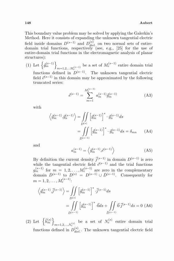
This boundary value problem may be solved by applying the Galerkin’sMethod. Here it consists of expanding the unknown tangential electricfield inside domains D(s−1) and D

(s)diel. on two normal sets of entire-

domain trial functions, respectively (see, e.g., [25] for the use ofentire-domain trial functions in the electromagnetic analysis of planarstructures):

(1) Let{~g

(s−1)m

}m=1,2,...M

(s−1)e

be a set of M(s−1)e entire domain trial

functions defined in D(s−1). The unknown tangential electricfield ~e(s−1) in this domain may be approximated by the followingtruncated series:

~e(s−1) =M

(s−1)e∑

m=1

a(s−1)m ~g(s−1)

m (A3)

with⟨~g(s−1)

m ,~g(s−1)n

⟩=

∫∫

D(s)

[~g(s−1)

m

]∗· ~g(s−1)

n ds

=∫∫

D(s−1)

[~g(s−1)

m

]∗· ~g(s−1)

n ds = δmn (A4)

anda(s−1)

m =⟨~g(s−1)

m ,~e(s−1)⟩

(A5)

By definition the current density ~j(s−1) in domain D(s−1) is zerowhile the tangential electric field ~e(s−1) and the trial functionsg(s−1)m for m = 1, 2, . . . ,M

(s−1)e are zero in the complementary

domain D(s−1) to D(s) = D(s−1) ∪ D(s−1). Consequently form = 1, 2, . . . , M

(s−1)e :

⟨~g(s−1)

m ,~j(s−1)⟩

=∫∫

D(s)

[~g(s−1)

m

]∗·~j(s−1)ds

=∫∫

D(s−1)

[~g(s−1)

m

]∗·~0ds +

∫∫

D(s−1)

~0·~j(s−1)ds = 0 (A6)

(2) Let{~h

(s)m

}m=1,2,...,N

(s)e

be a set of N(s)e entire domain trial

functions defined in D(s)diel.. The unknown tangential electric field


~e(s)diel in this domain may be represented by the following truncated

series:

~e(s)diel =

N(s)e∑

m=1

b(s)m

~h(s)m (A7)

with⟨~h(s)

m ,~h(s)n

⟩=

∫∫

D(s)

[~h(s)

m

]∗·~h(s)

n ds=∫∫

D(s)diel.

[~h(s)

m

]∗·~h(s)

n ds=δmn (A8)

andb(s)m =

⟨~h(s)

m , ~e(s)diel

⟩(A9)

By definition the current density ~j(s)diel in domain D

(s)diel. is zero

while the tangential electric field ~e(s)diel and the trial functions ~h

(s)m

for m = 1, 2, . . . , N(s)e are zero in the complementary domain D

(s)diel.

to D(s) = D(s)diel ∪ D

(s)diel. Consequently, for m = 1, 2, . . . , N

(s)e :

⟨~h(s)

m ,~j(s)diel

⟩=

∫∫

D(s)

[~h(s)

m

]∗·~j(s)

diel d s

=∫∫

D(s)diel

[~h(s)

m

]∗·~0 · d s +

∫∫

D(s)diel

~0 ·~j(s)diel d s = 0 (A10)

Moreover, following Section 2.4.1, the tangential electric field ~E(s) andthe current density ~J (s) inside the domain D(s) may be expanded onthe discrete normal set of modes

{~F

(s)n

}n=1,2,...

in this domain, that is:

~E(s) =∞∑

n=1

V (s)n

~F (s)n and ~J (s) =

N(s)∑

n=1

I(s)n

~F (s)n (A11)

With⟨

~F(s)m , ~F

(s)

n

⟩=

∫∫D(s)

[~F

(s)m

]∗·~F (s)

n ds = δmn. In Eq. (A11) the

quantities V(s)n and I

(s)n designate respectively the voltage and current

amplitudes of the n-th mode in D(s). Following Section 2.4.2, thetangential electric field ~E(s−1) and the current density ~J (s−1) inside

150 Aubert

the domain D(s−1) may be expanded on the discrete normal set ofmodes

{~F

(s−1)n

}n=1,2,...

in this domain, that is:

~E(s−1) =N(s−1)∑

n=1

V (s−1)n

~F (s−1)n and ~J (s−1) =

N(s−1)∑

n=1

I(s−1)n

~F (s−1)n (A12)

with⟨

~F(s−1)m , ~F

(s−1)

n

⟩=

∫∫D(s−1)

[~F

(s−1)m

]∗·~F (s−1)

n ds = δmn. In Eq. (A12)

V(s−1)n and I

(s−1)n designate respectively the voltage and current

amplitudes of the n-th mode in D(s−1). By applying the Galerkinmethod to the boundary value problem the following linear system ofequations is then derived:

[V (s)

][V (s−1)

]

[0][0]

=

[0] [0] [P ] [Q][0] [0] [R] [0]

− [P ]∗T − [R]∗T[Y

]11

[Y

]12

− [Q]∗T [0][Y

]21

[Y

]22

[I(s)

][I(s−1)

][a(s−1)

][a(s)

]

(A13)

where[V (scale)

]and

[I(scale)

](with scale = s, s−1) are column vectors

of the N (scale) elements V(scale)n and I

(scale)n respectively,

[a(s−1)

]is a

column vector of M(s−1)e elements a

(s−1)m ,

[a(s)

]is a column vector

of N(s)e elements b

(s)m ; [P ] is a N (s) × M

(s−1)e matrix of elements⟨

F(s)m , ~g(s−1)

n

⟩, [Q] is a N (s) × N

(s)e matrix of elements

⟨F

(s)m ,~h

(s)

n

⟩,

[R] is a N (s−1) × M(s−1)e matrix of elements

⟨F

(s−1)m , ~g(s−1)

n

⟩,

[Y

]11

is a M(s−1)e × M

(s−1)e matrix of elements

⟨~g

(s−1)m ,Y (s)~g

(s−1)n

⟩,

[Y

]12

is a M(s−1)e × N


⟨~g

(s−1)m ,Y (s)~h

(s)n

⟩,

[Y

]21

is a

N(s)e ×M

(s−1)e matrix of elements

⟨~h

(s)m ,Y (s)~g

(s−1)n

⟩and finally

[Y

]22

is a N(s)e × N


⟨~h

(s)m ,Y (s)~h

(s)n

⟩. From Eq. (A13)


the unknown column vectors[a(s−1)

]and

[a(s)

]may be expressed in

the following form:[ [

a(s−1)]

[a(s)

]]

=

[Y

]11

[Y

]12[

Y]21

[Y

]22

−1 [[P ]∗T [R]∗T

[Q]∗T [0]

][ [I(s)

][I(s−1)

]]

(A14)

Therefore: [V (s,s−1)

]= [P ]

[Y

]−1[P ]∗T

[I(s,s−1)

](A15)

with[

V (s,s−1)]

=[ [

V (s)]

[V (s−1)

]]

,[I(s,s−1)

]=

[ [I(s)

][I(s−1)

]]

, (A16)

[P ] =

[[P ] [Q][R] [0]

](A17)

and

[Y

]=

[Y

]11

[Y

]12[

Y]21

[Y

]22

(A18)

REFERENCES

1. Mittra, R., J.-F. Ma, E. Lucente, and A. Monorhio, “CBMOM— An iteration free MoM approach for solving large multiscaleEM radiation and scattering problems,” IEEE Antennas andPropagation Society International Symposium, Vol. 2B, 2–5,Washington, D.C., Jul. 3–8, 2005.

2. Lucente, E., A. Monorchio, and R. Mittra, “Generation ofcharacteristic basis functions by using sparse MoM impedancematrix to construct the solution of large scattering and radiationproblems,” IEEE Antennas and Propagation Society InternationalSymposium, 4091–4094, Albuquerque, New Mexico, Jul. 9–14,2006.

3. Nadarassin, M., H. Aubert, and H. Baudrand, “Analysis of planarstructures by an integral multi-scale approach,” IEEE MTT-SInternational Microwave Symposium, Vol. 2, 653–656, Orlando,Florida, USA, May 14–19, 1995.

152 Aubert

4. Baudrand, H. and S. Wane, Circuits Multi-echelles: Utilisationdes Sources Auxiliaires. Modelisation Caracterisation et Mesuresde Circuits Integres Passifs R.F, Vol. 3, 75–108, Hermes, 2003.

5. Baudrand, H., “Electromagnetic study of coupling between activeand passive circuits,” Microwave and Optoelectronics Conference,Vol. 1, 143–152, Aug. 11–14, 1997.

6. Perret, E., H. Aubert, and H. Legay, “Scale-Changing techniquefor the electromagnetic modelling of MEMS-controlled planarphase-shifters,” IEEE Trans. Microwave Theory and Tech.,Vol. 54, No. 9, 3594–3601, Sep. 2006.

7. Perret, E., N. Raveu, H. Aubert, and H. Legay, “Scale-Changingtechnique for MEMS-controlled phase-shifters,” 36th EuropeanMicrowave Week, 866–869, Manchester, United Kingdom,Sep. 10–15, 2006.

8. Voyer, D., H. Aubert, and J. David, “Scale-changing technique forthe electromagnetic modeling of planar self-similar structures,”IEEE Trans. Antennas Propagat., Vol. 54, No. 10, 2783–2789,Oct. 2006.

9. Voyer, D., H. Aubert, and J. David, “Radar cross section ofdiscrete self-similar objects using a recursive electromagneticanalysis,” IEEE Antennas and Propagation Society InternationalSymposium, Vol. 4, 4260–4263, Monterey, California, USA,Jun. 20–26, 2004.

10. Voyer, D., H. Aubert, and J. David, “Radar cross section ofself-similar targets,” Electronics Letters, Vol. 41, No. 4, 215–217,Feb. 17, 2005.

11. Perret, E. and H. Aubert, “Scale-Changing technique for thecomputation of the input impedance of active patch antennas,”IEEE Antennas and Wireless Propagation Letters, Vol. 4, 326–328, 2005.

12. Perret, E. and H. Aubert, “A multi-scale technique for theelectromagnetic modeling of active antennas,” IEEE Antennasand Propagation Society International Symposium, Vol. 4, 3923–3926, Monterey, California, USA, Jun. 20–25, 2004.

13. Raveu, N., G. Prigent, H. Aubert, P. Pons, and H. Legay,“Scale-Changing technique design and optimisation tool for activereflect-arrays cell,” 37th European Microwave Conference, 736–739, Munchen, Germany, Oct. 9–12, 2007.

14. Nathalie Raveu, E. Perret, Herve Aubert, and H. Legay, “Designof MEMS controlled phase shifter using SCT,” PIERS Online,Vol. 3, No. 2, 230–232, Beijing, China, Mar. 26–30, 2007.


15. Raveu, N., E. Perret, H. Aubert, and H. Legay, “Scale-changingtechnique: A design tool for reflectarrays active cells,” Proceedingsof the European Microwave Association, Vol. 4, No. 2, 163–168,Journal of the European Microwave Association, Jun. 2008.

16. Collin, R. E., Field Theory of Guided Waves, 2nd edition, IEEEPress, 1991.

17. Rozzi, T. E. and W. F. G. Mecklenbrauker, “Wide-band networkmodelling of interacting inductive irises and steps,” IEEE Trans.Microwave Theory and Tech., Vol. 23, No. 2, 235–245, Feb. 1975.

18. Tao, J. W. and H. Baudrand, “Multimodal variational analysisof uniaxial waveguide discontinuities,” IEEE Trans. MicrowaveTheory and Tech., Vol. 39, No. 3, 506–516, Mar. 1991.

19. Chew, W. C., Waves and Fileds in Inhomogeneous Media, IEEEPress, 1995.

20. Baudrand, H., “Representation by equivalent circuit of theintegral methods in microwave passive elements,” EuropeanMicrowave Conference, Vol. 2, 1359–1364, Budapest, Hungary,Sep. 10–13, 1990.

21. Baudrand, H., H. Aubert, D. Bajon, and F. Bouzidi, “Equivalentnetwork representation of boundary conditions involving gener-alized trial quantities,” Annals of Telecommunications, Vol. 52,No. 5–6, 285–292, 1997.

22. Baudrand, H., Introduction au Calcul des Elements de CircuitsPassifs en Hyperfrequences, Editions Cepadues, 2000.

23. Aubert, H. and H. Baudrand, L’electromagnetisme par lesSchemas Equivalents, Editions Cepadues, 2003.

24. Bouzidi, F., H. Aubert, D. Bajon, and H. Baudrand,“Equivalent network representation of boundary conditionsinvolving generalized trial quantities — Application to lossytransmission lines with finite metallization thickness,” IEEETrans. Microwave Theory and Tech., Vol. 45, 869–876, Jun. 1997.

25. Nadarassin, M., H. Aubert, and H. Baudrand, “Analysis of planarstructures by an integral approach using entire domain trialfunctions,” IEEE Trans. Microwave Theory and Tech., Vol. 10,2492–2495, Oct. 1995.

26. Larbi, C., A. Bouallegue, and H. Baudrand, “Utilisation d’unprocessus de renormalisation pour l’etude electromagnetiquedes structures fractales bidimensionnelles,” Annales desTelecommunications, Vol. 60, No. 7–8, 1023–1050, Juillet-Aout,2005.

27. Larbi, C., T. Ben Salah, T. Aguili, A. Bouallegue, and

154 Aubert

H. Baudrand, “Study of the Sierpinski’s Carpet fractal planarantenna by the renormalisation method,” International Journalof Microwave and Optical Technology, 58–65, 2005.

Documents

THE CONCEPT OF SCALE-CHANGING NETWORK IN THE GLOBAL