Research article

Effects of changing scale on landscape pattern analysis: scaling relations

Jianguo WuLandscape Ecology and Modeling Laboratory (LEML), Faculty of Ecology, Evolution, and EnvironmentalScience, School of Life Sciences, Arizona State University, Tempe, AZ 85287-1601, USA; (e-mail:Jingle.Wu@asu.edu)

Received 2 December 2002; accepted in revised form 20 August 2003

Key words: Landscape metrics, Pattern analysis, Scale effects, Scaling, Scalograms, Grain, Extent

Abstract

Landscape pattern is spatially correlated and scale-dependent. Thus, understanding landscape structure and func-tioning requires multiscale information, and scaling functions are the most precise and concise way of quantify-ing multiscale characteristics explicitly. The major objective of this study was to explore if there are any scalingrelations for landscape pattern when it is measured over a range of scales �grain size and extent�. The resultsshowed that the responses of landscape metrics to changing scale fell into two categories when computed at theclass level �i.e., for individual land cover types�: simple scaling functions and unpredictable behavior. Similarly,three categories were found at the landscape level, with the third being staircase pattern, in a previous studywhen all land cover types were combined together. In general, scaling relations were more variable at the classlevel than at the landscape level, and more consistent and predictable with changing grain size than with chang-ing extent at both levels. Considering that the landscapes under study were quite diverse in terms of both com-position and configuration, these results seem robust. This study highlights the need for multiscale analysis inorder to adequately characterize and monitor landscape heterogeneity, and provides insights into the scaling oflandscape patterns.

Introduction

Spatial heterogeneity is ubiquitous across all scalesand forms the fundamental basis of the structure andfunctioning of landscapes, be they natural or cultural.To understand how landscapes affect, and are affectedby, biophysical and socioeconomic activities, wemust be able to quantify spatial heterogeneity and itsscale dependence �i.e., how patterns change withscale�. Indeed, much of what has been done in geog-raphy, remote sensing and ecology has to do with de-scribing, manipulating, and understanding spatialheterogeneity. With the increasing recognition of theimportance of spatial heterogeneity by ecologists inthe past two decades, landscape ecology has come ofage with a distinctive emphasis on the spatial dimen-sion of ecological pattern and process �Turner et al.

2001; Wu and Hobbs 2002�. An important unifyingconcept in dealing with heterogeneity and integratingecological and geographical sciences is scale. Whilethe term “scale” may refer to any one or combinationsof several concepts, including grain �or resolution,support�, extent, lag �or spacing�, and cartographicratio �Wiens 1989; Lam and Quatrochi 1992;Schneider 2001; Dungan et al. 2002�, in this paper itrefers only to “grain” �the spatial resolution of a map�and “extent” �the map size, or “geographic scale” asdefined by Lam and Quatrochi 1992�.

The scale dependence of spatial heterogeneity hasbeen recognized in both geography and ecology fordecades. Two different but related connotations ofscale dependence of spatial heterogeneity may bedistinguished. The first implies that spatial heteroge-neity exhibits various patterns at different scales, or

© 2004 Kluwer Academic Publishers. Printed in the Netherlands.125Landscape Ecology 19: 125–138, 2004.

patterns have distinctive “operational” scales �sensuLam and Quattrochi 1992� at which they can be bestcharacterized. Apparently, this perspective is consis-tent with the concepts of characteristic scale and hi-erarchy that have been prevalent in ecologicalliterature since the 1980s �Allen and Starr 1982; Allenet al. 1984; O’Neill et al. 1986; Urban et al. 1987;Wu and Loucks 1995; Wu 1999�. The second conno-tation refers to the dependence of observed spatialheterogeneity on the scale of observation and analy-sis – often discussed in terms of scale effects on im-age classification and spatial pattern analysis. Scaleeffects have long been studied in human geographyas part of the modifiable areal unit problem or MAUP– the problem in spatial analysis that occurs whenarea-based data are aggregated �Openshaw 1984; Ar-bia et al. 1996; Jelinski and Wu 1996; Wrigley et al.1996; Marceau 1999�. MAUP includes two distinctbut related aspects: the result of statistical analysis isaffected by both the level of data aggregation or grainsize �so-called “scale problem”� and by alternativeways of aggregating pixels at a given grain size �of-ten called the “zoning problem” or “aggregationproblem”�. MAUP has frequently been discussed to-gether with the so-called “ecological fallacy” �sensuRobinson 1950� which refers to inappropriate extrap-olation of statistical relationships from one scale toanother. Unfortunately, the term “ecological fallacy”is misleading and can be irritating because the prob-lem it refers to occurs across all natural and socialsciences whenever heterogeneity and nonlinearity ex-ist and because the use of the term “ecological” hereis not at all scientifically rigorous. A more appropri-ate term for this kind of scale-related problems maybe “spatial transmutation” �sensu O’Neill 1979; alsosee King et al. 1991; Wu and Levin 1994�.

Scale effects on spatial pattern analysis may occurin each of the following three situations: �1� chang-ing grain size �or resolution� only, �2� changing ex-tent only, and �3� changing both grain and extent. Asnoted earlier, the modifiable areal unit probleminvolves both the effect of altered grain size and theway of this alteration. Similarly, there are also differ-ent ways of changing extent: e.g., boxing out from thecenter of a map or starting from one corner along adiagonal direction. In general, much more researchhas been done into the effects of changing grain size�particularly in the context of MAUP� than those ofchanging extent, and a quantitative understanding ofthese two kinds of scale effects across different sys-tems and methods is still lacking. Scale effects do not

necessarily have to be considered as problemsbecause they can be used for understanding the mul-tiple-scale characteristics of landscapes �Jelinski andWu 1996; Wu et al. 2000; Wu et al. 2003�. In prin-ciple, the relevant pattern is revealed only when thescale of analysis approaches the operational scale ofthe phenomenon under study �Allen et al. 1984; Wuand Loucks 1995; Wu 1999�. In practice, however,not all scale breaks revealed in multiscale analysis byresampling data correspond to actual operationalscales or hierarchical levels due to inaccuraciescaused by the methods of data aggregation andanalysis �Wu et al. 2000; Hay et al. 2001�.

While most of the MAUP studies prior to the1990’s focused on traditional statistical measures�e.g., mean, variance, regression and correlation co-efficients� and spatial interaction models, scale effectshave been increasingly studied using landscape met-rics �or indices� in ecology, remote sensing, and ge-ography in the past two decades �Meentemeyer andBox 1987; Turner et al. 1989; Turner et al. 2001; Bianand Walsh 1993; Moody and Woodcock 1994; Ben-son and Mackenzie 1995; Wickham and Riitters1995; Jelinski and Wu 1996; O’Neill et al. 1996; Qiand Wu 1996; Wu et al. 2003�. These studies haveshed new light on the problems of scale effects inpattern analysis as well as the multiscaled nature ofspatial heterogeneity. Yet, most of the existing stud-ies that used landscape metrics considered only a fewindices with a narrow range of scales, and few havegone beyond merely reporting the existence of scaleeffects to explore their generalities across differentlandscapes. Thus, although ecologists are well awarethat changing scale often affects landscape metrics,scaling relations are yet to be developed.

To systematically explore the effects of changingscale on pattern analysis, using simulated landscapeswith known structural characteristics is both neces-sary and effective �Gardner et al. 1987; Amrhein1995; Arbia et al. 1996; Hargis et al. 1998; Wu et al.2000; Saura and Martinez-Millan 2001�. However,comprehensive empirical studies using real landscapedata are needed because only such studies can tell uswhat kinds of scaling relations may exist and howvariable or consistent they are in actual �not justsimulated� landscapes. Such information is indispens-able for more in-depth and systematic investigationsusing simulated or artificially constructed landscapes.Therefore, this study was focused on data sets fromreal landscapes, while our results from simulatedlandscapes, which generally support findings here,

126

will be reported elsewhere. We also note that,although two general types of methods have beenused in landscape pattern analysis – spatial statistics�including geostatistics� and pattern metrics, this pa-per deals only with the second. Excellent reviews onspatial statistical methods and their applications canbe found in Rossi et al. �1992�, Goovaerts �1997�, andFortin �1999�. This study was designed to address thefollowing specific questions: �1� How do changinggrain size and changing extent affect different land-scape metrics for a given landscape? �2� How doesthe behavior of various landscape metrics differamong distinctive landscapes? �3� Are there generalscaling relations for certain landscape metrics that areconsistent across landscapes?

These questions need to be addressed using land-scape metrics computed both at the entire landscapelevel �taking account of all patch types altogether�and at the class level �each patch type being consid-ered separately�. Although many of the landscape-and class-level metrics are mathematically similar,their physical meanings are usually quite distinct �seeMcGarigal and Marks 1995�. While the landscape-level metrics are synoptic measures of the landscapeas a whole, the class-level metrics provide informa-tion on each patch �or land cover� type in the land-scape, which is necessary for most ecological orplanning considerations. Wu et al. �2003� examined19 landscape-level metrics based on five landscapedata sets �4 of them used here in this study�. This pa-pers focuses on 17 class-level metrics and comparesthe scaling relations at the levels of the individualpatch type and the whole landscape.

Data and methods

Seventeen class-level landscape metrics were exam-ined in this study: Class Area �CA�, Percent of Land-scape �CA%�, Number of Patches �NP�, PatchDensity �PD�, Total Edge �TE�, Edge Density �ED�,Largest Patch Index �LPI�, Mean Patch Size �MPS�,Patch Size Standard Deviation �PSSD�, Patch SizeCoefficient of Variation �PSCV�, Landscape ShapeIndex �LSI�, Mean Patch Shape Index �MPSI�, Area-Weighted Mean Shape Index �AWMSI�, Double-LogFractal Dimension �DLFD�, Mean Patch Fractal Di-mension �MPFD�, Area Weighted Mean Patch FractalDimension �AWMFD�, and Square Pixel �SqP�. Thesoftware package, FRAGSTATS 2.0 �McGarigal andMarks 1995�, was used to compute the selected land-

scape metrics, with Square Pixel Index �Frohn 1998�being added to the package by modifying the sourcecode.

Four land use and land cover maps with contrast-ing spatial patterns were used for this study: �A� aboreal forest landscape with 11 land use and landcover types including various forest stands, disturbedareas and water, �B� Minden landscape in the GreatBasin, USA with 15 land use and land cover types in-cluding native arid plant communities, burned areas,and urban and agricultural land uses, �C� Washoelandscape in the Great Basin, USA with 11 land useand land cover types most of which were shrublands,and �D� Phoenix urban landscape with 24 land useand land cover types, dominated by various urban andagricultural land uses. The boreal forest landscape inCanada showed little human disturbance, the twoGreat Basin landscapes in Nevada exhibited moder-ate urbanization and cultivation, and the metropolitanPhoenix landscape was a highly urbanized environ-ment. Land use and land cover types varied consid-erably across these landscapes in terms of both thenumber and the content of patch types. The spatialresolution of all data sets was 30 by 30 meters, andthe spatial extent varied from 357 km2 �630�630pixels� for the boreal landscape to 2025 km2

�1500�1500 pixels� for the Phoenix landscape. De-tails of these study areas have been given elsewhere�Wu et al. 2003; Luck and Wu 2002�.

To investigate the effects of changing grain size,the spatial resolution of three landscape maps �Boreal,Minden, and Phoenix� was systematically changedfrom 1 by 1 to 100 by 100 pixels with the extent keptconstant, which was consistent with Wu et al. �2003�.As the grain size increased, data were aggregated fol-lowing the majority rule, which is one of the mostcommonly used methods for aggregating categoricaldata in ecology and remote sensing. Each new map,with progressively larger grain size �e.g., 1�1, 2�2,..., 100�100�, was created by directly aggregating theoriginal data set, instead of using a cumulative pro-cedure that would introduce more errors. When thegrain size could not wholly divide the number of rowsor columns of the data set, the remainder of rows orcolumns at the edge were excluded from the newmap. This omission of edge rows and columns did notseem to be a problem as long as the extent/grain ratiowas sufficiently large. To investigate the effects ofchanging extent, we systematically increased the ex-tent of the maps diagonally starting from the north-

127

west corner while keeping the grain size constant �Wuet al. 2003�.

Results

Scaling relations with respect to changing grain size

With changing grain size through spatial aggregation,the responses of the 17 class-level metrics fell intotwo general groups: metrics showing consistent scal-ing relations �Type I� and metrics showing unpredict-able scaling behavior �Type II�. The first group wasfurther divided into those showing both consistentand robust scaling relations �Type IA� and thoseshowing consistent but less robust scaling relations�Type IB�. Note that the word “consistent” here refersto the consistence of scaling relations between differ-ent landscapes, whereas the word “robust” indicatesthe similarity of scaling relations between differentpatch types within the same landscape.

Figure 1 shows examples of how different metricsresponded to changing grain size for three studylandscapes in the form of scalograms, i.e., plots oflandscape metrics against scale �grain size or extent�.Table 1 is a summary of the scaling relations and theircharacteristics with respect to changing grain size. Ofthe 17 metrics, 5 belonged to Type IA: Number ofPatches �NP�, Patch Density �PD�, Total Edge �TE�,Edge Density �ED�, and Landscape Shape Index�LSI�; and 7 to Type IB: Largest Patch Index �LPI�,Square Pixel Index �SqP�, Mean Patch Size �MPS�,Patch Size Standard Deviation �PSSD�, Patch SizeCoefficient of Variation �PSCV�, Area-WeightedMean Shape Index �AWMSI�, and Area-WeightedMean Fractal Dimension �AWMFD�. Type IA metricsexhibited a power-law scaling relation which washighly consistent and robust over a range of scales,i.e.,

y � axb, a � 0, b � 0 �1�

where y is the value of a landscape metric, a and bare constants, and�is the grain size expressed as thenumber of pixels along a side.

Type IB metrics showed several different scalingrelations with a consistent “global pattern” betweendifferent landscapes, but rather high “short-rangevariations” between different patch types which may,in part, have been caused by the low abundance of

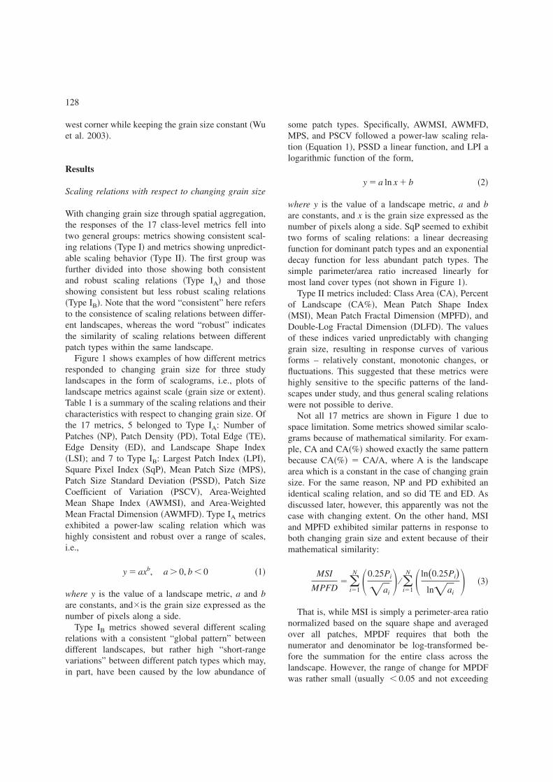
some patch types. Specifically, AWMSI, AWMFD,MPS, and PSCV followed a power-law scaling rela-tion �Equation 1�, PSSD a linear function, and LPI alogarithmic function of the form,

y � a ln x � b �2�

where y is the value of a landscape metric, a and bare constants, and x is the grain size expressed as thenumber of pixels along a side. SqP seemed to exhibittwo forms of scaling relations: a linear decreasingfunction for dominant patch types and an exponentialdecay function for less abundant patch types. Thesimple parimeter/area ratio increased linearly formost land cover types �not shown in Figure 1�.

Type II metrics included: Class Area �CA�, Percentof Landscape �CA%�, Mean Patch Shape Index�MSI�, Mean Patch Fractal Dimension �MPFD�, andDouble-Log Fractal Dimension �DLFD�. The valuesof these indices varied unpredictably with changinggrain size, resulting in response curves of variousforms – relatively constant, monotonic changes, orfluctuations. This suggested that these metrics werehighly sensitive to the specific patterns of the land-scapes under study, and thus general scaling relationswere not possible to derive.

Not all 17 metrics are shown in Figure 1 due tospace limitation. Some metrics showed similar scalo-grams because of mathematical similarity. For exam-ple, CA and CA�%� showed exactly the same patternbecause CA�%� � CA/A, where A is the landscapearea which is a constant in the case of changing grainsize. For the same reason, NP and PD exhibited anidentical scaling relation, and so did TE and ED. Asdiscussed later, however, this apparently was not thecase with changing extent. On the other hand, MSIand MPFD exhibited similar patterns in response toboth changing grain size and extent because of theirmathematical similarity:

MSI

MPFD� �

i�1

N �0.25Pi

�ai� ⁄ �

i�1

N �ln�0.25Pi�ln�ai

� �3�

That is, while MSI is simply a perimeter-area rationormalized based on the square shape and averagedover all patches, MPDF requires that both thenumerator and denominator be log-transformed be-fore the summation for the entire class across thelandscape. However, the range of change for MPDFwas rather small �usually � 0.05 and not exceeding

128

Figure 1. Examples of landscape metric scalograms with changing grain size: �A� a boreal forest landscape, �B� the Minden landscape, and�C� the central Phoenix urban landscape. The lines in each scalogram represent different patch types �i.e., land use and land cover types�.Landscape-level metrics �the thick black lines� are also plotted for comparison.

129

0.1� in both cases of changing grain size and extent,which made it less desirable for comparison. Simi-larly, the scale response curves of AWMSI and AW-MFD resembled each other because:

AWMSI ⁄ AWMFD � �i�1

N ��0.25Pi

�ai�

�ai

A�� ⁄ �i�1

N �ln�0.25Pi�ln�ai

�ai

A���4�

In this case, AWMFD seemed more preferable be-cause it was bale to suppress somewhat the abruptlarge fluctuations that occurred with AWMSI, so thata comparison between patch types became more fea-sible.

Scaling relations with respect to changing extent

The responses of class-level metrics to changing ex-tent could also be classified into two groups: Type Imetrics showing consistent and relatively robust scal-ing relations and Type II metrics with unpredictablescaling behavior �Table 2 and Figure 2�. Type I met-rics included NP, TE, LSI, SqP, and CA, whereas theother 12 belonged to Type II. NP, TE, and CA exhib-ited a power law scaling relation that was consistentbetween different landscapes but varied noticeablybetween patch types within the same landscape. Withincreasing extent, SqP increased rapidly initially andthen began to approach a maximum value, whereasLSI tended to increase continuously. For relativelyabundant patch types, a logarithmic function for SqPand a linear scaling function for LSI could beobtained by regression. These trends seemed consis-

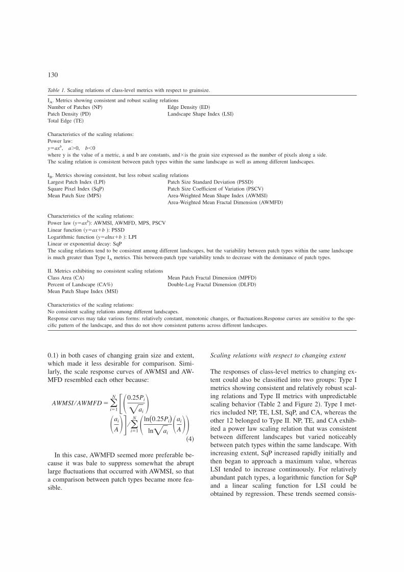
Table 1. Scaling relations of class-level metrics with respect to grainsize.

IA. Metrics showing consistent and robust scaling relationsNumber of Patches �NP� Edge Density �ED�Patch Density �PD� Landscape Shape Index �LSI�Total Edge �TE�

Characteristics of the scaling relations:Power law:y�axb, a�0, b�0where y is the value of a metric, a and b are constants, and�is the grain size expressed as the number of pixels along a side.The scaling relation is consistent between patch types within the same landscape as well as among different landscapes.

IB. Metrics showing consistent, but less robust scaling relationsLargest Patch Index �LPI� Patch Size Standard Deviation �PSSD�Square Pixel Index �SqP� Patch Size Coefficient of Variation �PSCV�Mean Patch Size �MPS� Area-Weighted Mean Shape Index �AWMSI�

Area-Weighted Mean Fractal Dimension �AWMFD�

Characteristics of the scaling relations:Power law �y�axb�: AWMSI, AWMFD, MPS, PSCVLinear function �y�ax�b �: PSSDLogarithmic function �y�alnx�b �: LPILinear or exponential decay: SqPThe scaling relations tend to be consistent among different landscapes, but the variability between patch types within the same landscapeis much greater than Type IA metrics. This between-patch type variability tends to decrease with the dominance of patch types.

II. Metrics exhibiting no consistent scaling relationsClass Area �CA� Mean Patch Fractal Dimension �MPFD�Percent of Landscape �CA%� Double-Log Fractal Dimension �DLFD�Mean Patch Shape Index �MSI�

Characteristics of the scaling relations:No consistent scaling relations among different landscapes.Response curves may take various forms: relatively constant, monotonic changes, or fluctuations.Response curves are sensitive to the spe-cific pattern of the landscape, and thus do not show consistent patterns across different landscapes.

130

tent among different landscapes, and the variabilitybetween patch types tended to decrease with the in-creasing abundance of patch types. The responsecurves of Type II metrics showed no consistent scal-ing patterns, and were highly dependent upon thespecifics of the landscapes.

Overall, the effects of changing extent on land-scape metrics were much less predictable than thoseof changing grain size. This was evident from twofacts: �1� the number of Type I metrics was muchsmaller for changing extent than for changing grainsize �5 vs. 12�; and �2� Type I metrics for grain sizewere less variable than those for extent between patchtypes and among landscapes. Several differences be-tween changing grain size and extent are noteworthy.Unlike in the case of changing grain size, PD and EDdid not show any consistent scaling functionsalthough their behavioral patterns seemed to resembleeach other. As grain size increased, PSSD tended toincrease linearly, while PSCV declined and MPS in-creased both in a power-law fashion. In contrast, asextent increased, MPS changed unpredictably, butwith a much smaller magnitude than in the case ofchanging grain size. Thus, PSSD and PSCV bothtended to increase in a similar way for most landcover types �PSCV = PSSD/MPS�. This was most ob-vious for the boreal landscape, in which the behav-

ioral patterns of PSSD and PSCV resembled eachother closely because MPS changed little over theentire range of extent.

BecauseLSI�0.25TE⁄�TA �where TA is the totalarea of the landscape�, LSI and TE behaved the sameway in response to changing grain size. However, inthe case of changing extent, if TE increases as apower function �y�axb� with extent �measured as thenumber of pixels on a side�, LSI should follow a scal-ing function of the form,y�xb�1. Then, if b is close to2, then LSI should behave nearly linearly. Our resultsindeed showed that for most patch types LSI tendedto increase linearly, but with considerable variations.The deviations of the observed patterns for LSI froma linear function were attributable to the considerablyvariable scale responses of TE. Also, LSI and SqP arenumerically related to each other, i.e.,LSI��1�SqP��1. Thus, the response curves of LSI and SqP re-flected this relationship. Both of them showed muchgreater variations, and thus less predictability, be-tween patch types and among landscapes in the caseof changing extent. Another interesting finding wasthat DLFD, for most patch types, was unpredictableand varied increasingly with increasing grain size, butappeared to be relatively constant with continuing in-crease in extent after initial fluctuations at smallerscales. The latter was reminiscent of the notion that

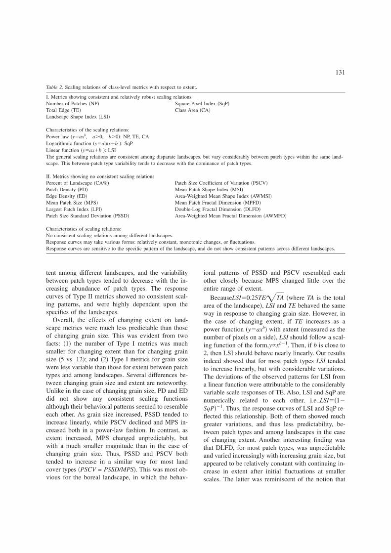
Table 2. Scaling relations of class-level metrics with respect to extent.

I. Metrics showing consistent and relatively robust scaling relationsNumber of Patches �NP� Square Pixel Index �SqP�Total Edge �TE� Class Area �CA�Landscape Shape Index �LSI�

Characteristics of the scaling relations:Power law �y�axb, a�0, b�0�: NP, TE, CALogarithmic function �y�alnx�b �: SqPLinear function �y�ax�b �: LSIThe general scaling relations are consistent among disparate landscapes, but vary considerably between patch types within the same land-scape. This between-patch type variability tends to decrease with the dominance of patch types.

II. Metrics showing no consistent scaling relationsPercent of Landscape �CA%� Patch Size Coefficient of Variation �PSCV�Patch Density �PD� Mean Patch Shape Index �MSI�Edge Density �ED� Area-Weighted Mean Shape Index �AWMSI�Mean Patch Size �MPS� Mean Patch Fractal Dimension �MPFD�Largest Patch Index �LPI� Double-Log Fractal Dimension �DLFD�Patch Size Standard Deviation �PSSD� Area-Weighted Mean Fractal Dimension �AWMFD�

Characteristics of scaling relations:No consistent scaling relations among different landscapes.Response curves may take various forms: relatively constant, monotonic changes, or fluctuations.Response curves are sensitive to the specific pattern of the landscape, and do not show consistent patterns across different landscapes.

131

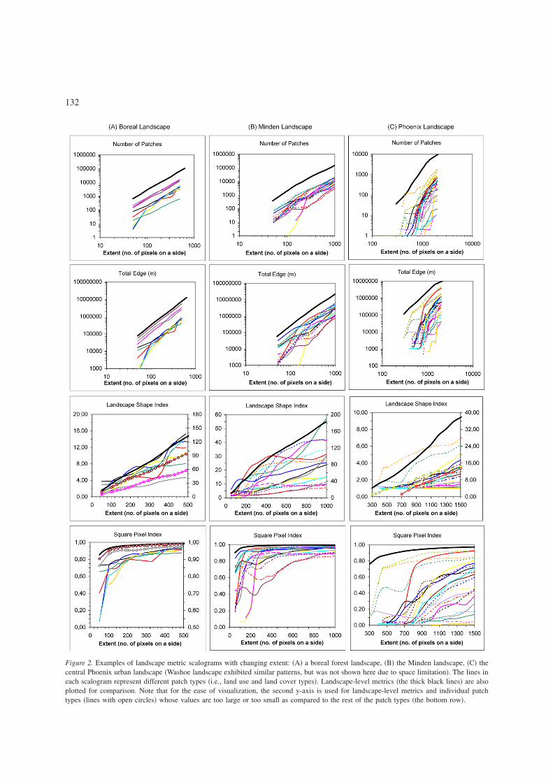
Figure 2. Examples of landscape metric scalograms with changing extent: �A� a boreal forest landscape, �B� the Minden landscape, �C� thecentral Phoenix urban landscape �Washoe landscape exhibited similar patterns, but was not shown here due to space limitation�. The lines ineach scalogram represent different patch types �i.e., land use and land cover types�. Landscape-level metrics �the thick black lines� are alsoplotted for comparison. Note that for the ease of visualization, the second y-axis is used for landscape-level metrics and individual patchtypes �lines with open circles� whose values are too large or too small as compared to the rest of the patch types �the bottom row�.

132

landscapes may exhibit self-similarity over a finiterange of spatial extent �Milne 1991; Milne 1992; Lamand Quatrochi 1992�.

Discussion

Comparing scaling relations of class- andlandscape-level metrics

In a related study, Wu et al. �2003� showed that theresponses of 19 landscape-level metrics to changinggrain size and extent could be categorized as threegeneral types: �1� Type I metrics exhibiting consistentand robust scaling relations in the forms of linear,power, or logarithmic functions over a range ofscales; �2� Type II metrics showing staircase-like re-sponses with changing scale; and �3� Type III metricsbehaving erratically in response to changing scale andwith no consistent scaling relations among differentlandscapes. In the case of changing grain size, 12metrics belonged to Type I: NP, PD, TE, ED, LSI,AWMSI, AWMFD, PSCV, MPS, SqP, PSSD, and

LPI; 3 to Type II: PR �Patch Richness�, PRD �PatchRichness Density�, and SHDI �Shannon’s DiversityIndex�; and 4 to Type III: DLFD, CONT �Contagion�,MPFD, and MSI. In the case of changing extent, thenumber of Type I metrics reduced to 6: NP, TE, SqP,PRD, SHDI, and LSI; the number of Type II metricswas 5: PR, PSSD, PSCV, AWMSI, and AWMFD; andthe number of Type III metrics increased to 8: PD,ED, DLFD, MPS, LPI, CONT, MSI, and MPFD. Inaddition, Wu et al. �2003� showed that the startingposition and the direction of changing extent couldalso significantly influence the scaling patterns forcertain landscape metrics.

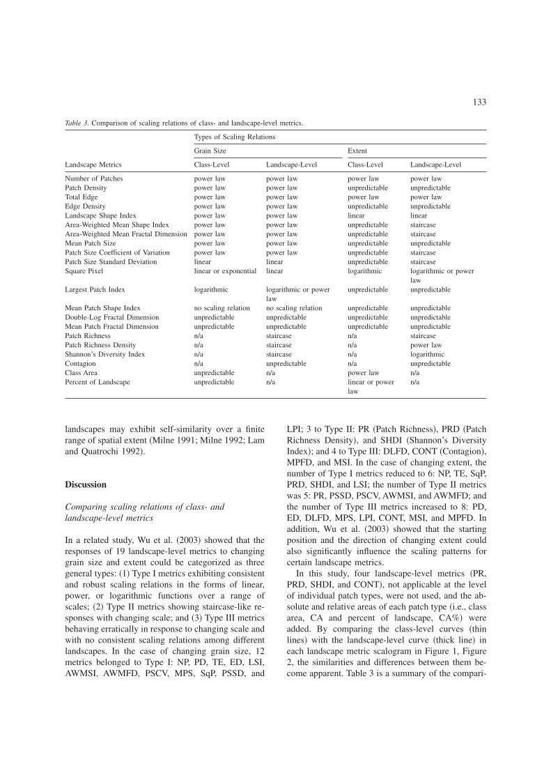
In this study, four landscape-level metrics �PR,PRD, SHDI, and CONT�, not applicable at the levelof individual patch types, were not used, and the ab-solute and relative areas of each patch type �i.e., classarea, CA and percent of landscape, CA%� wereadded. By comparing the class-level curves �thinlines� with the landscape-level curve �thick line� ineach landscape metric scalogram in Figure 1, Figure2, the similarities and differences between them be-come apparent. Table 3 is a summary of the compari-

Table 3. Comparison of scaling relations of class- and landscape-level metrics.

Types of Scaling Relations

Grain Size Extent

Landscape Metrics Class-Level Landscape-Level Class-Level Landscape-Level

Number of Patches power law power law power law power lawPatch Density power law power law unpredictable unpredictableTotal Edge power law power law power law power lawEdge Density power law power law unpredictable unpredictableLandscape Shape Index power law power law linear linearArea-Weighted Mean Shape Index power law power law unpredictable staircaseArea-Weighted Mean Fractal Dimension power law power law unpredictable staircaseMean Patch Size power law power law unpredictable unpredictablePatch Size Coefficient of Variation power law power law unpredictable staircasePatch Size Standard Deviation linear linear unpredictable staircaseSquare Pixel linear or exponential linear logarithmic logarithmic or power

lawLargest Patch Index logarithmic logarithmic or power

lawunpredictable unpredictable

Mean Patch Shape Index no scaling relation no scaling relation unpredictable unpredictableDouble-Log Fractal Dimension unpredictable unpredictable unpredictable unpredictableMean Patch Fractal Dimension unpredictable unpredictable unpredictable unpredictablePatch Richness n/a staircase n/a staircasePatch Richness Density n/a staircase n/a power lawShannon’s Diversity Index n/a staircase n/a logarithmicContagion n/a unpredictable n/a unpredictableClass Area unpredictable n/a power law n/aPercent of Landscape unpredictable n/a linear or power

lawn/a

133

son of scaling relations between the class andlandscape levels. The same 15 metrics used at boththe class and landscape levels showed rather similarscaling patterns in terms of both the specific metricsand the scaling relations. In general, effects of chang-ing grain size were more predictable than changingextent in that more metrics showed consistent scalingrelations across different landscapes in the formercase. However, it must be emphasized here that arti-facts due to data aggregation and consequent analysismay become overwhelming for classes with ex-tremely low abundance. Because of the high between-patch type variability at the class level, the staircase-like responses of such metrics as AWMSI, AWMFD,PSCV, and PSSD with respect to changing extent ap-peared consistent only at the landscape level.

It is important to note that this study only used oneof the several methods of aggregating spatial data –the majority rule method. Although this may be themost commonly used one in ecological and remotesensing applications, it would be interesting to com-pare how different aggregation methods affect thecharacteristics of landscape metric scalograms. Anumber of studies have shown that different aggrega-tion methods may have significant effects on spatialmodel evaluation, land cover classification, and land-scape pattern analysis �Costanza 1989; Justice et al.1989; Bian and Butler 1999; Turner et al. 2001�.Thus, aggregation methods may also affect scalingrelations of landscape metrics.

Scale multiplicity of landscapes and multiscalepattern analysis

The relationship between pattern and scale has beena central issue in ecology and geography �MacArthur1972; Meentemeyer 1989; Levin 1992; Wu andLoucks 1995�. Pattern is rooted in spatial heterogene-ity which in turn stems from variations of spatial de-pendence. The first law in geography – “Everythingis related to everything else, but near things are morerelated than distant things” �sensu Tobler 1970� – isessentially a law of spatial autocorrelation. However,heterogeneity manifests itself as patchiness and gra-dients intertwined over a wide range of spatial scales.Thus, scale dependence is as essential a property ofheterogeneity as is spatial dependence. This has ledto the claim of “the second law in geography” �sensuArbia et al. 1996�: “Everything is related to every-thing else, but things observed at a coarse spatialresolution are more related than things observed at a

finer resolution.” This is simply a law of scale depen-dence of correlation, which was developed based onboth empirical and analytical results that the correla-tion between variables increases while variancedecreases as the resolution �grain size� of spatial datais increased �Amrhein 1995; Arbia et al. 1996; Wu etal. 2000�. Of course, not only are correlation coeffi-cients and variance scale dependent, so are a varietyof landscape indices, statistical methods, and mathe-matical models as well.

Many, if not most, landscapes are hierarchicallystructured �Urban et al. 1987; Woodcock and Har-ward 1992; Wu and Loucks 1995; Reynolds and Wu1999; Wu 1999�. Even before hierarchy theorybecame an influential perspective in ecology and be-fore multi-scale pattern analyses became commonlypracticed in earth sciences, the eminent ecologistRobert MacArthur �1972� already unambiguously re-cognized the scale multiplicity and hierarchical natureof landscapes, as he said: “A real environment has ahierarchical structure. That is to say, it is like acheckerboard of habitats, each square of which has,on closer examination, its own checkerboard structureof component subhabitats. And even the tiny squaresof these component checkerboards are revealed asthemselves checkerboards, and so on. All environ-ments have this kind of complexity, but not all haveequal amounts of it.”

To understand the structure and functioning oflandscapes, therefore, the scale dependence of spatialheterogeneity must be quantified. Recent develop-ments in landscape ecology have provided a new im-petus as well as a suite of innovative theories andmethods for achieving this goal �Turner et al. 2001;Wu and Hobbs 2002�. To identify the characteristicscales or hierarchical levels of landscape structure,two general approaches are available. The first is touse statistical methods that are inherently multi-scaled, such as semivariance analysis �Burrough1995�, wavelet analysis �Bradshaw and Spies 1992�,spectral analysis �Platt and Denman 1975�, fractalanalysis �Milne 1997�, lacunarity analysis �Plotnick etal. 1993�, and scale variance �Moellering and Tobler1972; Wu et al. 2000�. The second is, as illustrated inthis study, to construct scalograms using simple mea-sures such as landscape metrics computed progres-sively over a series of scales and then to explorescaling functions. Spatial statistical methods havebeen known for their ability to detect characteristicscales, and, in particular, semivariance analysis hasbeen frequently used for this purpose. However, re-

134

cent studies have indicated that in semivariograms ofreal landscapes fine-scale variability can be“squeezed” by broad-scale variability, so that multi-scale structure may be obscured �Meisel and Turner1998; Wu et al. 2000�. In addition, the results ofsemivariance analysis and their interpretations canalso be significantly affected by changing the grainsize, lag, and extent of the data sets �Dungan et al.2002�.

Can landscape metrics detect hierarchical struc-tures of landscapes when repeatedly computed atmultiple scales? Apparently, not all of them can. Ourearlier study showed that progressively increasingextent allowed certain landscape metrics �e.g., PSCV,PSSD, MPS, AWMSI, AWMFD� to reflect some dra-matic shifts in the average properties of the landscapeconcerning the size and shape of patches �Table 3; Wuet al. 2003�. Other studies also demonstrated thatsimple variance and correlation measures were ableto detect scale breaks in real and artificial landscapeswhen calculated at different grain sizes �e.g., O’Neillet al. 1991; Wu et al. 2000�. Nevertheless, there areat least three reasons for the lack of scale breaks inthe landscape metric scalograms in this and othersimilar studies. First, when grain size is increased al-ways in a square shape following the majority rule,the hierarchical structure in real landscapes may bedistorted or masked because of the high variability inpatch size, shape and orientation �Wu et al. 2000�.This problem may be ameliorated by a “patch-based”or “object-specific” aggregation scheme �Hay et al.2001�. Second, different landscape metrics representdifferent aspects of landscape structure, and for agiven landscape not all of them exhibit hierarchicalstructure although they may all be scale-dependent.Third, even for landscape attributes that do posses hi-erarchical structure, be it structural or functional, theymay form multiple hierarchies in the same landscapewhich may not correspond to each other precisely interms of spatial and temporal scales �Wu 1999�.While the first reason is primarily methodological, thelast two involve both the theory of hierarchical sys-tems and the understanding of the systems understudy.

Spatial allometry and landscape pattern

It is intriguing that several metrics were found to ex-hibit power scaling relationships which were ostensi-bly consistent between different classes within thesame landscape and among different landscapes.

Other measures of landscape pattern that were notconsidered in this study may also scale spatially in apower law fashion. For example, Costanza and Max-well �1994� found that with increasing spatial resolu-tion �i.e., decreasing grain size�, the spatial auto-predictability �the reduction in uncertainty about thestate of a pixel in a scene given knowledge of the sateof adjacent pixels in that scene� increases and spatialcross-predictability �the reduction in uncertaintyabout the state of a pixel in a scene given knowledgeof the state of corresponding pixels in other scenes�decreases both linearly on a log-log scale. From thisstudy, it is evident that power-law scaling is more of-ten and more consistent in the case of changing grainsize than changing extent. It is attempting to relatethese landscape metric scaling relations to otherpower laws in biological and ecological systems –particularly, body-size allometry �biological attributesscale with body size following a power law; e.g.,Brown et al. 2000� and spatial allometry �ecologicalattributes scale with ecosystem size or spatial extentfollowing a power function; e.g., Schneider 2000�.The power, elegance, and mystery of allometric scal-ing all lie in the simple equation, y�axb, where thedependent variable y is a biological or an ecologicalvariable of interest,�is mostly body size in traditionalbiological allometry or a spatial scale measure �e.g.,grain, extent, or their ratio�, a is the normalizationconstant, and b is the scaling exponent. Thus, thepower laws of landscape metrics may be consideredas an extension of spatial allometry.

Do the power scaling relations in this study neces-sarily imply that a single underlying process isresponsible for the landscape attributes these metricsrepresent? Our knowledge of these rather differentlandscapes suggests that a number of natural and an-thropogenic processes, operating on distinctive spatialand temporal scales, have generated these landscapepatterns. Does this, then, suggest that multiplicativeprocesses can give rise to seemingly scale-invariantlandscape patterns with simple allometric scaling re-lations and no characteristic scales? These arecertainly intriguing questions that still await futureresearch. Although power laws have frequently beenrelated directly to, or cast in the light of, self-similar-ity, scale-invariance, and universality, such interpre-tations need to be made with caution. Power lawsmay arise from different processes, either internal orexternal to the system under consideration �Jensen1998; Plotnick and Sepkoski 2001�, and they usually

135

hold only over a finite ranges of spatiotemporal scales�Wiens 1989; Milne 1991; Milne 1992; Lam andQuatrochi 1992; Wu 1999�. More in-depth discus-sions on these issues as well as other scaling theoriesand methods are given in Wu et al. �2004�.

Conclusions

Landscape metrics have been widely used in ecologi-cal and geographical studies and provided valuableinsight into the structural characteristics of complexlandscapes. However, the lack of a comprehensiveunderstanding of the scale sensitivity of these metricsseriously undermines their interpretation and useful-ness. This study has systematically investigated howlandscape metrics respond to changing grain size andextent, allowing for exploration of general scaling re-lations and idiosyncratic behaviors.

The results of this study showed that changinggrain size and extent had significant effects on boththe class- and landscape-level metrics. Although thelandscapes under study were quite different in boththe composition and configuration of patches, the ef-fects of changing scale fell into two categories�simple scaling functions and unpredictable� for theclass-level metrics, and three categories for the land-scape-level metrics �simple scaling functions, stair-case-like scaling behavior, and unpredictable�. Over-all, more metrics showed consistent scaling relationswith changing grain size than with changing extent atboth the class and landscape levels – indicating thateffects of changing spatial resolution are generallymore predictable than those of changing map sizes.While the same metrics tended to behave similarly atthe class level and the landscape level, the scale re-sponses at the class level were much more variable.These results appear robust not only across differentlandscapes, but also independent of specific mapclassification schemes.

This study corroborates the increasingly recog-nized notions: there is no single “correct” or “opti-mal” scale for characterizing spatial heterogeneity,and comparison between landscapes using pattern in-dices must be based on the same spatial resolutionand extent. In addition, these results may providepractical guidelines for scaling of spatial pattern. Forexample, landscape metrics with simple scaling rela-tions reflect those landscape features that can be ex-trapolated or interpolated across spatial scales readilyand accurately using only a few data points. In con-

trast, unpredictable metrics represent landscape fea-tures whose extrapolation is difficult, which requiresinformation on the specifics of the landscape of con-cern at many different scales. Finally, to quantifyspatial heterogeneity using landscape metrics, it isboth necessary and desirable to use landscape metricscalograms, in stead of single-scale values. Indeed, acomprehensive empirical database containing patternmetric scalograms and other forms of multiple-scaleinformation of diverse landscapes is crucial forachieving a general understanding of landscape pat-terns and developing spatial scaling rules.

Acknowledgments

I would like to thank C. Overton, W. Shen, L. Zhangand M. A. Luck for their assistance with data prepa-ration and analysis. Comments from three anonymousreviewers improved the paper and were greatlyappreciated. This research was supported in part bygrants from the United States Department of Agricul-ture �USDA-NRICGP 95-37101-2028�, the U.S. En-vironmental Protection Agency’s Science to AchieveResults program �R827676-01-0�, and US NationalScience Foundation �DEB 97-14833, CAP-LTER�.

References

Allen T.F.H. and Starr T.B. 1982. Hierarchy: Perspectives for Eco-logical Complexity. University of Chicago Press, Chicago, Illi-nois, USA.

Allen R.F.H., O’Neill R.V. and Hoekstra T.W. 1984. Interlevel re-lations in ecological research and management. USDA ForestService Gen. Tech. Rep. RM-110, Rocky Mountain Forest andRange Experiment Station.

Amrhein C.G. 1995. Searching for the elusive aggregation effect:evidence from statistical simulations. Environment and PlanningA 27: 105–119.

Arbia G., Benedetti R. and Espa G. 1996. Effects of the MAUP onimage classification. Geogr. Syst. 3: 123–141.

Benson B.J. and Mackenzie M.D. 1995. Effects of sensor spatialresoltuion on landscape structure parameters. Landscape Ecol-ogy 10: 113–120.

Bian L. and Walsh S.J. 1993. Scale dependencies of vegetation andtopography in a mountainous environment of Montana. Profes-sional Geographer 45: 1–11.

Bian L. and Butler R. 1999. Comparing effects of aggregationmethods on statistical and spatial properties of simulated spatialdata. Photogrammatic Engineering and Remote Sensing 65: 73–84.

Bradshaw G.A. and Spies T.A. 1992. Characterizing canopy gapstructure in forests using wavelet analysis. Journal of Ecology80: 205–215.

136

Brown J.H. and West G.B. �ed.�, 2000. Scaling in Biology. OxfordUniversity Press, New York, New York, USA.

Burrough P.A. 1995. Spatial aspects of ecological data. In: Jong-man R.H.G., Ter Braak C.J.F. and Van Tongeren O.F.R. �eds�,Data Analysis in Community and Landscape Ecology. pp. 213-265. Cambridge University Press, Cambridge, UK.

Costanza R. 1989. Model goodness of fit – A multiple resolutionprocedure. Ecological Modelling 47: 199–215.

Costanza R. and Maxwell T. 1994. Resolution and predictability:An approach to the scaling problem. Landscape Ecology 9: 47–57.

Dale M.R.T. 1999. Spatial Pattern Analysis in Plant Ecology.Cambridge University Press, Cambridge, UK.

Dungan J.L., Perry J.N., Dale M.R.T., Legendre P., Citron-PoustyS., Fortin M.-J., Jakomulska A., Miriti M. and Rosenberg M.S.2002. A balanced view of scale in spatial statistical analysis. Ec-ography 25: 626–640.

Fortin M.J. 1999. Spatial statistics in landscape ecology. In: Klo-patek J.M. and Gardner R.H. �eds�, Landscape EcologicalAnalysis. pp. 253-279. Springer-Verlag, New York, New York,USA.

Frohn R.C. 1998. Remote Sensing for Landscape Ecology. LewisPublishers, Boca Raton, Florida, USA.

Gardner R.H., Milne B.T., Turner M.G. and O’Neill R.V. 1987.Neutral models for the analysis of broad-scale landscape pattern.Landscape Ecology 1: 19–28.

Goovaerts P. 1997. Geostatistics for Natural Resources Evaluation.Oxford University Press, New York, New York, USA.

Gustafson E.J. 1998. Quantifying landscape spatial pattern: Whatis the state of the art? Ecosystems 1: 143–156.

Hargis C.D., Bissonette J.A. and David J.L. 1998. The behavior oflandscape metrics commonly used in the study of habitat frag-mentation. Landscape Ecology 13: 167–186.

Hay G., Marceau D.J., Dubé P. and Bouchard A. 2001. A multi-scale framework for landscape analysis: Object-specific analysisand upscaling. Landscape Ecology 16: 471–490.

Jelinski D.E. and Wu J. 1996. The modifiable areal unit problemand implications for landscape ecology. Landscape Ecology 11:129–140.

Jensen H.J. 1998. Self-Organized Criticality: Emergent ComplexBehavior in Physical and Biological Systems. Cambridge Uni-versity Press, New York, New York, USA.

Justice C.O., Markham B.L., Townshend J.R.G. and Kennard R.L.1989. Spatial degradation of satellite data. International Journalof Remote Sensing 10: 1539–1561.

Keeling M.J., Mezic I., Hendry R.J., McGlade J. and Rand D.A.1997. Characteristic length scales of spatial models in ecologyvia fluctuation analysis. Philosophical Transactions of the RoyalSociety �London B� 352: 1589–1601.

King A.W., Johnson A.R. and O’Neill R.V. 1991. Transmutationand functional representation of heterogeneous landscapes.Landscape Ecology 5: 239–253.

Lam N.S.-N. and Quattrochi D.A. 1992. On the issues of scale,resolution, and fractal analysis in the mapping sciences. Profes-sional Geographer 44: 88–98.

Levin S.A. 1992. The problem of pattern and scale in ecology.Ecology 73: 1943–1967.

Luck M. and Wu J. 2002. A gradient analysis of urban landscapepattern: A case study from the Phoenix metropolitan region, Ari-zona, USA. Landscape Ecology 17: 327–339.

MacArthur R.H. 1972. Geographical Ecology: Patterns in the Dis-tribution of Species. Princeton University Press, Princeton, NewJersey, USA.

Marceau D.J. 1999. The scale issue in social and natural sciences.Canadian Journal of Remote Sensing 25: 347–356.

McGarigal K. and Marks B.J. 1995. FRAGSTATS: Spatial PatternAnalysis Program for Quantifying Landscape Structure. Gen.Tech. Rep. PNW-GTR-351. Pacific Northwest research Station.

Meentemeyer V. and Box E.O. 1987. Scale effects in landscapestudies. In: Turner M.G. �ed.�, Landscape Heterogeneity andDisturbance. pp. 15-34. Springer-Verlag, New York, New York,USA.

Meentemeyer V. 1989. Geographical perspectives of space, time,and scale. Landscape Ecology 3: 163–173.

Meisel J.E. and Turner M.G. 1998. Scale detection in real and ar-tificial landscapes using semivariance analysis. Landscape Ecol-ogy 13: 347–362.

Milne B.T. 1991. Heterogeneity as a multiscale characteristic oflandscapes. In: Kolasa J. and Pickett S.T.A. �eds�, EcologicalHeterogeneity. pp. 69-84. Springer-Verlag, New York, NewYork, USA.

Milne B.T. 1992. Spatial aggregation and neutral models in fractallandscapes. American Naturalist 139: 32–57.

Milne B.T. 1997. Applications of fractal geometry in wildlife biol-ogy. In: Bissonette J.A. �ed.�, Wildlife and Landscape Ecology:Effects of Pattern and Scale. pp. 32-69. Springer-Verlag, NewYork, New York, USA.

Moellering H. and Tobler W. 1972. Geographical variances. Geo-graphical Analysis 4: 34–64.

Moody A. and Woodcock C.E. 1994. Scale-dependent errors in theestimation of land-cover proportions: Implications for globalland-cover datasets. Photogrammatic Engineering and RemoteSensing 60: 585–594.

O’Neill R.V. 1979. Transmutations across hierarchical levels. In:Innis G.S. and O’Neill R.V. �eds�, Systems Analysis of Ecosys-tems. pp. 59-78. International Co-operative, Fairland, Maryland,USA.

O’Neill R.V., DeAngelis D.L., Waide J.B. and Allen T.F.H. 1986.A Hierarchical Concept of Ecosystems. Princeton UniversityPress, Princeton, New Jersey, USA.

O’Neill R.V., Gardner R.H., Milne B.T., Turner M.G. and JacksonB. 1991. Heterogeneity and spatial hierarchies. In: Kolasa J. andPickett S.T.A. �eds�, Ecological Heterogeneity. pp. 85-96.Springer-Verlag, New York, New York, USA.

O’Neill R.V., Hunsaker C.T., Timmins S.P., Timmins B.L., Jack-son K.B., Jones K.B., Riitters K.H. and Wickham J.D. 1996.Scale problems in reporting landscape pattern at the regionalscale. Landscape Ecology 11: 169–180.

Openshaw S. 1984. The Modifiable Areal Unit Problem. GeoBooks, Norwich, UK.

Platt T. and Denman K.L. 1975. Spectral analysis in ecology. An-nual Review of Ecology & Systematics 6: 189–210.

Plotnick R.E., Gardner R.H. and O’Neill R.V. 1993. Lacunarity in-dices as measures of landscape texture. Landscape Ecology 8:201–211.

Plotnick R.E. and Sepkoski J.J. 2001. A multiplicative multifractalmodel for originations and extinctions. Paleobiology 27:126–139.

Qi Y. and Wu J. 1996. Effects of changing spatial resolution on theresults of landscape pattern analysis using spatial autocorrelationindices. Landscape Ecology 11: 39–49.

137

Reynolds J.F. and Wu J. 1999. Do landscape structural and func-tional units exist? In: Tenhunen J.D. and Kabat P. �eds�, Inte-grating Hydrology, Ecosystem Dynamics, and Biogeochemistryin Complex Landscapes. pp. 273-296. Wiley, Chichester, UK.

Robinson A.H. 1950. Ecological correlation and the behaviour ofindividuals. Am. Soc. Rev. 15: 351–357.

Rossi R.E., Mulla D.J., Journel A.G. and Franz E.H. 1992. Geo-statistical tools for modeling and interpreting ecological spatialdependence. Ecological Monographs 62: 277–314.

Saura S. and Martinez-Millan J. 2001. Sensitivity of landscapepattern metrics to map spatial extent. Photogrammatic Engineer-ing and Remote Sensing 67: 1027–1036.

Schneider D.C. 2001. Spatial allometry. In: Gardner R.H., KempW.M., Kennedy V.S. and Petersen J.E. �eds�, Scaling Relationsin Experimental Ecology. pp. 113-153. Columbia UniversityPress, New York, New York, USA.

Schneider D.C. 2001. The rise of the concept of scale in ecology.BioScience 51: 545–553.

Tobler W. 1970. A computer movie simulating urban growth in theDetroit region. Econ. Geogr. �Suppl.� 46: 234–240.

Turner M.G., O’Neill R.V., Gardner R.H. and Milne B.T. 1989. Ef-fects of changing spatial scale on the analysis of landscape pat-tern. Landscape Ecology 3: 153–162.

Turner S.J., O’Neill R.V., Conley W., Conley M.R. and HumphriesH.C. 1991. Pattern and scale: Statistics for landscape ecology.In: Turner M.G. and Gardner R.H. �eds�, Quantitative Methodsin Landscape Ecology. pp. 17-49. Springer-Verlag, New York,New York, USA.

Turner M.G., Gardner R.H. and O’Neill R.V. 2001. LandscapeEcology in Theory and Practice: Pattern and Process. Springer-Verlag, New York, New York, USA.

Urban D.L., O’Neill R.V. and Shugart H.H. 1987. Landscape ecol-ogy: A hierarchical perspective can help scientists understandspatial patterns. BioScience 37: 119–127.

Wickham J.D. and Riitters K.H. 1995. Sensitivity of landscapemetrics to pixel size. International Journal of Remote Sensing16: 3585–3595.

Wiens J.A. 1989. Spatial scaling in ecology. Functional Ecology 3:385–397.

Woodcock C. and Harward V.J. 1992. Nested-hierarchical scenemodels and image segmentation. International Journal of RemoteSensing 13: 3167–3187.

Wrigley N., Holt T., Steel D. and Tranmer M. 1996. Analysing,modeling, and resolving the ecological fallacy. In: Longley P.and Batty M. �eds�, Spatial Analysis: Modellign in a GIS Envi-ronment. pp. 23-40. GeoInformation International, Cambridge,UK.

Wu J. and Levin S.A. 1994. A spatial patch dynamic modeling ap-proach to pattern and process in an annual grassland. EcologicalMonographs 64�4�: 447–464.

Wu J. and Loucks O.L. 1995. From balance-of-nature to hierarchi-cal patch dynamics: A paradigm shift in ecology. Quarterly Re-view of Biology 70: 439–466.

Wu J. 1999. Hierarchy and scaling: Extrapolating informationalong a scaling ladder. Canadian Journal of Remote Sensing 25:367–380.

Wu J., Jelinski D.E., Luck M. and Tueller P.T. 2000. Multiscaleanalysis of landscape heterogeneity: Scale variance and patternmetrics. Geogr. Info. Sci. 6: 6–19.

Wu J. and Hobbs R. 2002. Key issues and research priorities inlandscape ecology: An idiosyncratic synthesis. Landscape Ecol-ogy 17: 355–365.

Wu J., Shen W., Sun W. and Tueller P.T. 2003. Empirical patternsof the effects of changing scale on landscape metrics. LandscapeEcology 17: 761–782.

Wu J., Jones B., Li H. and Loucks O. L. �ed.�, 2004. Scaling andUncertainty Analysis in Ecology. Columbia University Press,New York, New York, USA �in press�.

138