The Clinical Effect of Changing from a Dose to Water to a

The Clinical Effect of Changing from a Dose to Water to a Dose to Medium-Based Methodology to Calculate Monitor

Units for Electron Beams

Hilary Frances Todd

Thesis submitted for the degree of

Master of Philosophy

School of Physical Sciences

University of Adelaide

September 2020

ii

Table of Contents

Table of Contents ..................................................................................................................... ii

List of Tables ............................................................................................................................. v

List of Figures ........................................................................................................................ viii

List of Abbreviations .............................................................................................................. xii

Abstract .................................................................................................................................. xiv

Declaration ............................................................................................................................. xvi

Acknowledgements .............................................................................................................. xvii

1 Introduction ....................................................................................................................... 1

2 Literature review ............................................................................................................... 4

2.1 Electron dose calculation algorithms ............................................................................................ 4

2.1.1 A historical perspective ................................................................................................. 4

2.1.2 Monte Carlo methods ................................................................................................... 5

2.1.3 Monitor units ................................................................................................................. 7

2.1.4 Dose to water versus dose to medium ......................................................................... 9

2.1.5 The Elekta Monaco® eMC algorithm ........................................................................... 11

2.2 Acute toxicity ............................................................................................................................... 15

3 Validation of dose to water in the Elekta Monaco® eMC algorithm in a homogeneous plastic water phantom .................................................................................................... 18

3.1 Introduction ................................................................................................................................. 18

3.2 Materials and methods ................................................................................................................ 19

3.2.1 Radiation detector....................................................................................................... 19

3.2.2 Homogeneous plastic water phantom ........................................................................ 20

3.2.3 Electrometer ............................................................................................................... 21

3.2.4 Electron beam energies .............................................................................................. 21

3.2.5 Creation of treatment plans ........................................................................................ 21

3.2.6 Phantom set-up and measurements ........................................................................... 22

3.2.7 Dose calculation formalism (𝐷𝑤) ............................................................................... 23

3.2.8 Electron dosimetry considerations in plastic phantoms .............................................. 25

iii

3.3 Results ........................................................................................................................................ 28

3.3.1 Validation of the CC04 ionisation chamber for use in electron beams ....................... 28

3.3.2 Optimal dose calculation parameters and export format ............................................ 29

3.3.3 Determination of the physical density, depth-scaling and fluence-scaling factors ...... 29

3.3.4 Comparison between Elekta Monaco® eMC dose calculations and measured 𝐷𝑤 in the homogeneous plastic water phantom ......................................................................... 31

3.4 Discussion ................................................................................................................................... 33

3.5 Conclusions ................................................................................................................................ 35

4 Validation of dose to medium in the Elekta Monaco® eMC algorithm in tissue equivalent slab phantoms................................................................................................................. 36

4.1 Introduction ................................................................................................................................. 36


4.2.1 Radiation detector....................................................................................................... 37

4.2.2 Tissue equivalent slab phantoms ............................................................................... 37

4.2.3 Electrometer ............................................................................................................... 40

4.2.4 Electron beam energies .............................................................................................. 41

4.2.5 Creation of treatment plans ........................................................................................ 41

4.2.6 Phantom set-up and measurements (for both simple and complex cases) ................ 42

4.2.7 Dose calculation formalism (𝐷𝑚) ............................................................................... 43

4.3 Results ........................................................................................................................................ 47

4.3.1 Overall depth-scaling factors for each tissue equivalent slab type ............................. 47

4.3.2 Comparison between Elekta Monaco® eMC dose calculations and measured 𝐷𝑚 in the simple phantoms......................................................................................................... 51

4.3.3 Comparison between Elekta Monaco® eMC dose calculations and measured 𝐷𝑚 in the complex phantom ....................................................................................................... 55

4.4 Discussion ................................................................................................................................... 57

4.5 Conclusions ................................................................................................................................ 60

5 Statistical analysis of patient acute toxicity data ......................................................... 62

5.1 Introduction ................................................................................................................................. 62


5.2.1 Patient data collection and summary statistics ........................................................... 63

5.2.2 Cochran-Armitage test for linear trend........................................................................ 67

5.2.3 Binary logistic regression models ............................................................................... 69

5.3 Results ........................................................................................................................................ 72

5.3.1 Summary statistics ...................................................................................................... 72

5.3.2 Cochran-Armitage test for linear trend........................................................................ 81

5.3.3 Binary logistic regression models ............................................................................... 82

5.4 Discussion ................................................................................................................................... 90

5.4.1 Baseline toxicity predictor variable ............................................................................. 92

iv

5.4.2 Cohort predictor variable ............................................................................................ 93

5.4.3 Tissue category predictor variable .............................................................................. 93

5.4.4 Future directions ......................................................................................................... 94

5.5 Conclusions ................................................................................................................................ 95

6 Response to research questions................................................................................... 96

6.1 Response to research question 1 ............................................................................................... 96

6.2 Response to research question 2 ............................................................................................... 96

7 References ...................................................................................................................... 98

v

List of Tables

Table 2.1: Compositions used by the Elekta Monaco® eMC dose calculation engine based on the

RED of individual voxels (Elekta 2014). .......................................................................................... 14

Table 3.1: Values of the depth-scaling factor, fluence-scaling factor (ℎ𝑝𝑙) and physical density for

various plastic types, reproduced from Table 7.VI of IAEA TRS-398 (Andreo et al. 2006). ............ 26

Table 3.2: Values of the depth-scaling factor, fluence-scaling factor and physical density for the IBA

IMRT phantom (RW3 plastic). 1The fluence-scaling factor was taken from IAEA TRS-398 as a “best

match” to Solid water® (RMI-457). .................................................................................................. 31

Table 3.3: Differences between the Elekta Monaco® eMC DFw dose calculations and the measured

𝐷𝑤 in the IMRT phantom for all electron beams (normalised to the maximum DFw calculated dose).

Difference values exceeding 3% are highlighted in red. ................................................................. 32

Table 4.1: The various tissue equivalent slabs used for depth-dose measurements and their

nominal physical densities. ............................................................................................................. 38

Table 4.2: The tissue substitutes used to obtain Spencer-Attix stopping power data for each tissue

equivalent slab type and the equivalent tissue substitute used in the Elekta Monaco® eMC

algorithm. ........................................................................................................................................ 47

Table 4.3: The ODSFs obtained for each tissue equivalent slab type and each electron energy. The

ODSFs were determined by applying various factors to the physical measurement depths until the

root mean square error between the PDIs measured in water and the PDIs measured in each of the

tissue equivalent slab phantoms was minimised. ........................................................................... 50

vi

Table 4.4: Differences between the Elekta Monaco® eMC 𝐷𝑚 dose calculations and the 𝐷𝑚 as

measured in the simple, tissue equivalent slab phantoms for all electron beam energies

(normalised to the maximum 𝐷𝑚 calculated dose). Difference values exceeding 7% are highlighted

in red, while those between 3 - 7% are highlighted in orange. ........................................................ 54


measured in the complex, inhomogeneous tissue equivalent slab phantom for 12 MeV and 15 MeV

(normalised to the maximum 𝐷𝑚 calculated dose). Difference values between 3 - 7% are

highlighted in orange. Also shown are the differences between the Elekta Monaco® eMC dose

calculations in terms of 𝐷𝑚 and 𝐷𝑤 (normalised to the maximum 𝐷𝑚 calculated dose). ............ 56

Table 5.1: Definitions of cohort 1 and cohort 2. .............................................................................. 64

Table 5.2: Definitions of skin-related adverse events, taken from CTCAE Version 4 (U.S

Department of Health and Human Services 2009). ........................................................................ 66

Table 5.3: General definitions of severity grades, taken from CTCAE Version 4 (U.S Department of

Health and Human Services 2009), where *Instrumental ADL refer to preparing meals, shopping for

groceries or clothes, using the telephone, managing money, etc. and **Self-care ADL refer to

bathing, dressing and undressing, feeding self, using the toilet, taking medications, and not

bedridden. ....................................................................................................................................... 66

Table 5.4: Basic clinical and treatment characteristics of patients recruited into the cohort study.. 73

Table 5.5: Incidence of radiation-induced acute skin toxicity for all adverse events combined. ..... 75

Table 5.6: The percentage of patients experiencing either no toxicity or maximum acute toxicity

grades of 1 to 5, in each cohort and for each adverse event. ......................................................... 77

Table 5.7: p-values from the Cochran-Armitage test for linear trend, as calculated in Genstat, for

each individual adverse event and for all events combined. ........................................................... 82

Table 5.8: A summary of results from the binary logistic regression models for each adverse event.

Significant results are highlighted in green. .................................................................................... 85

vii

Table 5.9: The number of outliers (i.e. normalised residuals with an absolute value larger than 2.6)

in the binary logistic regression models for each adverse event. .................................................... 89

viii

List of Figures

Figure 2.1: Electron beam transport from the source phase space to the exit phase space plane

(reproduced from Elekta (2014)). .................................................................................................... 12

Figure 3.1: A transverse slice through the IBA IMRT phantom used for depth-dose measurements

with the CC04 cylindrical ionisation chamber. The particular slice shown is positioned at the centre

of the ionisation chamber slot (shown by the red contour). ............................................................. 20

Figure 3.2: PDD measurements using the Roos® plane parallel chamber and the CC04 ionisation

chamber in water for all electron beam energies. The Elekta Monaco® eMC DFw calculated data are

also shown for reference................................................................................................................. 28

Figure 3.3: PDD measurements using the CC04 ionisation chamber in water and in the IMRT

phantom for all electron energies. The customised ODSF of 0.98 has been applied to the physical

measurement depths in the IMRT phantom. ................................................................................... 30

Figure 3.4: Comparisons of Elekta Monaco® eMC DFw dose calculations and the measured 𝐷𝑤

(using the CC04 ionisation chamber) in the IMRT phantom for all electron beams. The customised

ODSF of 0.98 has been applied to the physical measurement depths in the IMRT phantom. ........ 32

Figure 4.1: The various tissue equivalent slabs used for depth-dose measurements. Top left:

adipose; Top right: exhale lung; Bottom left: trabecular bone; Bottom right: cortical bone. ............. 38

Figure 4.2: The adipose homogeneous tissue equivalent slab phantom as used for depth-dose

measurements. ............................................................................................................................... 39

Figure 4.3: The complex, inhomogeneous tissue equivalent slab phantom as used for depth-dose

measurements. ............................................................................................................................... 40

ix

Figure 4.4: PDI measurements using the CC04 ionisation chamber in water (solid green curve) and

in the simple, adipose phantom (solid red curve) for all electron energies. Also plotted is the PDI

data as measured in the simple, adipose phantom with the optimal ODSF applied to the physical

measurement depths (dashed red curve). ...................................................................................... 48


in the simple, exhale lung phantom (solid red curve) for all electron energies. Also plotted is the PDI

data as measured in the simple, exhale lung phantom with the optimal ODSF applied to the

physical measurement depths (dashed red curve). ........................................................................ 48


in the simple, trabecular bone phantom (solid red curve) for all electron energies. Also plotted is the

PDI data as measured in the simple, trabecular bone phantom with the optimal ODSF applied to

the physical measurement depths (dashed red curve). .................................................................. 49


in the simple, cortical bone phantom (solid red curve) for all electron energies. Also plotted is the

PDI data as measured in the simple, cortical bone phantom with the optimal ODSF applied to the

physical measurement depths (dashed red curve). ........................................................................ 49

Figure 4.8: Comparison of the Elekta Monaco® eMC 𝐷𝑚 dose calculation and the 𝐷𝑚 as

measured in the simple, adipose phantom for all electron beam energies. .................................... 51


measured in the simple, exhale lung phantom for all electron beam energies. ............................... 52


measured in the simple, trabecular bone phantom for all electron beam energies. ........................ 52


measured in the simple, cortical bone phantom for all electron beam energies. ............................. 53

x


measured in the complex, inhomogeneous tissue equivalent slab phantom for 12 MeV and 15 MeV.

For reference, Elekta Monaco® eMC 𝐷𝑤 data are also shown. ..................................................... 56

Figure 5.1: The use of binary logistic regression in the context of this statistical analysis (image

modified from Scale (2020)). ........................................................................................................... 70

Figure 5.2: The percentage of patients treated for different anatomical sites in cohort 1 and cohort

2. ..................................................................................................................................................... 74

Figure 5.3: The difference between the measured 𝐷𝑤-based MU and the 𝐷𝑚-based MU as

calculated in the Elekta Monaco® eMC algorithm (data only applicable to patients in cohort 1). .... 75

Figure 5.4: The percentage of patients in each cohort experiencing either no toxicity or maximum

acute skin toxicity grades of 1 to 5 for the rash adverse event. ...................................................... 78


acute skin toxicity grades of 1 to 5 for the infection adverse event. ................................................ 78


acute skin toxicity grades of 1 to 5 for the pain adverse event. ....................................................... 79


acute skin toxicity grades of 1 to 5 for the telangiectasia adverse event......................................... 79


acute skin toxicity grades of 1 to 5 for the soft tissue fibrosis adverse event. ................................. 80


acute skin toxicity grades of 1 to 5 for the alopecia adverse event. ................................................ 80


acute skin toxicity grades of 1 to 5 for the skin ulceration adverse event. ....................................... 81

Figure 5.11: Scatter plot (taken from the IBM® SPSS software output) of the raw residuals against

the predicted probability for the rash adverse event. ...................................................................... 86

xi


the predicted probability for the infection adverse event. ................................................................ 86


the predicted probability for the pain adverse event. ...................................................................... 87


the predicted probability for the telangiectasia adverse event. ....................................................... 87


the predicted probability for the soft tissue fibrosis adverse event. ................................................. 88


the predicted probability for the alopecia adverse event. ................................................................ 88


the predicted probability for the skin ulceration adverse event. ...................................................... 89

xii

List of Abbreviations

AAPM The American Association of Physicists in Medicine

ARPANSA The Australian Radiation Protection and Nuclear Safety Agency

BCC Basal cell carcinoma

CI Confidence interval

CIRS Computerised Imaging Reference Systems Inc.

CTCAE Common Terminology Criteria for Adverse Events

DFw Dose forced to water

𝐷𝑚 Dose to medium

DVH Dose-volume histogram

𝐷𝑤 Dose to water

eMC Electron Monte Carlo

eMR Electronic medical record

EPID Electronic portal imaging device

ESTAR Stopping power and range tables for electrons

IAEA The International Atomic Energy Agency

ICRP The International Commission on Radiological Protection

ICRU The International Commission on Radiation Units and Measurements

IGRT Image guided radiation therapy

IMRT Intensity modulated radiation therapy

xiii

MNCCI The Mid North Coast Cancer Institute

MU Monitor units

NIST National Institute of Standards and Technology

NTCP Normal tissue complication probability

ODSF Overall depth scaling factor

PDD Percentage depth dose

PDI Percentage depth ionisation

RED Relative electron density

SCC Squamous cell carcinoma

STOPS Simultaneous Transport of Particle Steps

TCP Tumour control probability

TG-51 The AAPM TG-51 protocol for clinical reference dosimetry of high-energy

photon and electron beams

TPS Treatment planning system

TRS-398 The IAEA international Code of Practice for dosimetry based on standards

of absorbed dose to water (Technical Report Series No. 398)

xiv

Abstract

In 2016, The Mid North Coast Cancer Institute (MNCCI) implemented Elekta’s Monaco® electron

Monte Carlo (eMC) dose calculation algorithm for electron beams. The new algorithm resulted in a

change in clinical practice whereby monitor units (MU) delivered to patients would be calculated in

terms of dose to medium (𝐷𝑚), rather than using measured, dose to water (𝐷𝑤)-based MU.

Delivering high energy ionising radiation during radiotherapy has inherent risks. Therefore, it is crucial

to patient safety that dose calculations performed by the treatment planning system (TPS) are

accurate. Any changes in clinical practice should also be understood in terms of their effect on patient

outcomes (both tumour control and normal tissue toxicity). This research aims to validate the

accuracy of the 𝐷𝑚-based MU calculated by the Elekta Monaco® eMC algorithm and to assess

patient outcomes in terms of acute skin toxicity due to this change in clinical practice.

To validate the 𝐷𝑚-based MU, the dose measured with an ionisation chamber was compared with

the dose calculated by the Elekta Monaco® eMC algorithm in a range of clinically relevant phantoms.

The assessment of acute toxicity involved a cohort study that compared acute skin toxicity grades of

skin cancer patients treated before the change in clinical practice (cohort 1) and after the change

(cohort 2). Various predictors of radiation-induced acute skin toxicity were also investigated.

The comparison between measured and calculated dose found that the Elekta Monaco® eMC 𝐷𝑚

calculation is accurate in most clinical scenarios. The level of agreement between the measured and

calculated 𝐷𝑚 data is mostly within ± 3.5% for a wide range of tissue types. However, for tissues

xv

with densities significantly different from water (i.e. < 0.5 g/cm3 and > 1.5 g/cm3), the method used to

determine 𝐷𝑚 from measurements of ionisation resulted in unacceptable levels of uncertainty. For

these tissues, a more accurate validation method, such as full Monte Carlo modelling, is required.

Two hundred and ninety-four patients were recruited into the cohort study, with 141 patients in cohort

1 and 153 patients in cohort 2. Statistical analysis of patient acute toxicity data was performed using

the Cochran-Armitage test for linear trend and binary logistic regression modelling.

The results of the Cochran-Armitage test for linear trend found no statistically significant increase in

acute skin toxicity for patients in cohort 2 compared with patients in cohort 1. Therefore, the change

in clinical practice from using the measured 𝐷𝑤-based MU to using the 𝐷𝑚-based MU as calculated

in the Elekta Monaco® eMC algorithm does not increase acute skin toxicity for skin cancer patients

treated with electron beams.

Binary logistic regression modelling found a statistically significant correlation between baseline

toxicity grade and acute toxicity grade, suggesting that baseline grade is often a predictor of acute

toxicity grade. This modelling also found that patients treated with the 𝐷𝑚-based MU as calculated

in the Elekta Monaco® eMC algorithm experience statistically significant lower levels of pain, while

those patients with treatment sites involving bone experience statistically significant lower levels of

pain but increased alopecia.

xvi

Declaration

I certify that this work contains no material which has been accepted for the award of any other

degree or diploma in my name, in any university or other tertiary institution and, to the best of my

knowledge and belief, contains no material previously published or written by another person, except

where due reference has been made in the text. In addition, I certify that no part of this work will, in

the future, be used in a submission in my name, for any other degree or diploma in any university or

other tertiary institution without the prior approval of the University of Adelaide and where applicable,

any partner institution responsible for the joint-award of this degree.

I give permission for the digital version of my thesis to be made available on the web, via the

University’s digital research repository, the Library Search and also through web search engines,

unless permission has been granted by the University to restrict access for a period of time.

I acknowledge the support I have received for my research through the provision of an Australian

Government Research Training Program Scholarship.

Hilary Frances Todd Date

04/09/2020

xvii

Acknowledgements

Thank you to my supervisors at The University of Adelaide, Dr Scott Penfold, Dr Michael Douglass

and Dr Judith Pollard for their advice and support over the past four years. I would like to pay

particular thanks to Scott for his understanding and technical assistance early on, helping a lost soul

navigate, for the first time, the complicated world of medical physics. It was reassuring to know that

someone was there, at the end of the phone, to help with those early experiments. Thank you.

Thanks go also to my local supervisor, Dr Brendan Chick, for his useful discussions on my research

project and for feedback on this thesis.

For help with the challenging world of statistics, I was grateful to have the expertise of Dr Ivan Iankov.

Thank you for your enthusiasm and your advice – it enabled me to take this project to the next level.

I would like to acknowledge my place of employment, The Mid North Coast Cancer Institute, NSW

Health, for letting me take on this clinical project. In particular, I would like to thank the radiation

oncologists who purchased the equipment used in this project, and thank Brett Waller, for putting

together the equipment purchase proposal.

Thank you to the patients, of whom their anonymised data was used to create clinical relevance in

this project. I hope that, in some small way, it will benefit the future patients that we treat.

xviii

I would also like to thank two special people. Firstly, Pam: you made sure I was well stocked with

countless bags of lollies, coffee and bottles of Cognac. Thank you for your brilliant ideas and for

passing on to me your love of writing. I can proudly say that this thesis has been officially “Pammed”.

Secondly, Sean: it is impossible to describe the sacrifices you made and the work you did so this

thesis could be completed. From my trusty physics lab assistant, to my cook, cleaner, barista and

bartender—your intelligence and patience never cease to amaze me. I hope never to burden you

ever again with discussions on monitor units, depth-scaling factors or binary logistic regression

models.

This thesis is dedicated to baby Esperance

1

1 Introduction

Cancer is a leading cause of mortality in Australia with close to 50,000 deaths estimated for 2019

(Australian Institute of Health and Welfare 2019). It is expected that 150,000 new cases of cancer

will be diagnosed in Australia in 2020, representing an increase of almost 40% since 2007 (Australian

Institute of Health and Welfare 2012). Radiotherapy is a common form of treatment, used in

approximately 50% of notifiable cancer cases in Australia (Ingham Institute for Applied Medical

Research 2013), either with curative intent or for palliation. It uses high energy ionising radiation to

damage the DNA of cancer cells, ultimately leading to cell death.

An essential component of a modern-day radiotherapy department is the treatment planning system

(TPS). A TPS allows planners to tailor treatments to the specific anatomy of the patient and design

beam arrangements to maximise radiation damage to the tumour volume while sparing normal tissue.

However, high energy ionising radiation has inherent risks. It is crucial, therefore, to patient safety

that the dose calculations performed by the TPS are accurate. Furthermore, dose calculations play

a critical role in optimising the therapeutic gain by maximising the tumour control probability (TCP)

while minimising the normal tissue complication probability (NTCP). In fact, studies have shown that

a 5% change in dose can result in a 10% - 20% change in TCP or up to a 20% - 30% change in

NTCP (Chetty et al. 2007; Goitein & Busse 1975; Stewart & Jackson 1975).

Dose calculation algorithms for electron beams have evolved dramatically over the years: from

rudimentary broad beam approaches to pencil beam techniques, and, more recently, to Monte Carlo

methods. Monte Carlo-based algorithms are increasingly used for their superior calculation accuracy,

2

particularly in inhomogeneous tissue, as compared with analytic dose algorithms. A major implication

of Monte Carlo-based treatment planning systems is that doses can be calculated with respect to the

actual tissue in which they are deposited i.e. dose to medium (𝐷𝑚).

To improve treatment accuracy, in 2016, The Mid North Coast Cancer Institute (MNCCI) implemented

Elekta’s Monaco® electron Monte Carlo (eMC) dose calculation algorithm for electron beams. Upon

initial clinical implementation, the monitor units (MU) delivered to the patient were based on a cut-out

factor measurement in plastic water, according to previous MNCCI practice. However, from

approximately May 2018, clinical practice changed whereby the 𝐷𝑚-based MU as calculated in the

Elekta Monaco® eMC algorithm were used for all patient treatments.

MNCCI staff noted the number of MU calculated in the Elekta Monaco® eMC algorithm in terms of

𝐷𝑚 were higher, on average, compared with the MU based on measurements in plastic water. For

some treatment sites involving significant tissue inhomogeneities, large differences (of approximately

10%) were observed, similar to that reported in the literature (Cygler et al. 2005). Some radiation

oncologists at MNCCI queried whether the magnitude of these differences in MU would clinically

affect patient outcomes.

Acute toxicity is one radiobiological measure that can be used to judge the effect of this change in

clinical practice. Acute toxicity results from the death of a large number of cells and occurs within a

few days or weeks after irradiation. Many studies have investigated the severity of acute toxicity due

to various changes in clinical practice (Lin et al. 2018; McDonald et al. 2016). However, to date, little

work has been carried out to assess acute skin toxicity variations when changing to a Monte Carlo

𝐷𝑚-based treatment planning approach for clinical electron beams. Given the differences between

the 𝐷𝑚-based MU as calculated in the Elekta Monaco® eMC algorithm and those derived from water-

3

based measurement, a clinically observable increase in acute skin toxicity due to this change in

clinical practice is plausible.

To address the queries raised by the radiation oncologists, this research project aims to answer two

key research questions.

Research question 1: Are the 𝐷𝑚-based MU as calculated in the Elekta Monaco® eMC algorithm

accurate in a range of clinically relevant settings?

Research question 2: Is there a clinically observable increase in acute skin toxicity for electron

patients treated with the Elekta Monaco® eMC 𝐷𝑚-based MU as compared with a similar cohort of

patients treated with the measured dose to water (𝐷𝑤)-based MU?

Both Chapter 3 and Chapter 4 address research question 1. Chapter 3 investigates the ability of the

Elekta Monaco® eMC algorithm to accurately predict 𝐷𝑤 in simple scenarios involving a

homogeneous plastic water phantom. Chapter 4 builds further on the Elekta Monaco® eMC algorithm

validation through dosimetric studies involving the measurement of 𝐷𝑚 in tissue equivalent slab

phantoms. These chapters also outline the dosimetry calculation system used to obtain accurate

absorbed dose measurements in plastic phantoms in terms of both 𝐷𝑤 and 𝐷𝑚.

Chapter 5 addresses research question 2 through a statistical analysis of acute toxicity data for skin

cancer patients treated with electron beams at MNCCI. It involves a cohort study to determine if there

is a statistically significant difference in patient acute skin toxicity due to the change in clinical

practice. Various predictors of radiation-induced acute skin toxicity are also investigated.

4

2 Literature review

This chapter explores the literature in two key areas: electron dose calculation algorithms and acute

toxicity. Electron dose calculation algorithms are explained from their rudimentary beginnings to the

advanced techniques used in modern-day radiotherapy departments. A particular focus is on Monte

Carlo techniques, with the Elekta Monaco® eMC algorithm explained in depth. The use of 𝐷𝑤 versus

𝐷𝑚 in Monte Carlo treatment planning is also discussed. The radiobiological basis of acute toxicity,

along with various acute toxicity classification schemes are outlined. A brief summary of published

acute toxicity studies is provided, highlighting a gap in the current literature. This gap framed the

basis for research question 2.

2.1 Electron dose calculation algorithms

2.1.1 A historical perspective

Historically, patient dose calculations for electron beams have been carried out using broad-beam

methods and more recently using the pencil-beam approach. Broad-beam dose calculation

algorithms involved 1D ray-tracing with manual scaling of isodose curves in regions of inhomogeneity

(Mayles, Nahum & Rosenwald 2007). This simplistic methodology was problematic due to its

limitations in accurately modelling irregular fields and inhomogeneities. These limitations are

particularly pronounced for electron beams due to dose in the build-up region at the patient surface

and the effects of lateral scatter around tissue inhomogeneities.

5

Pencil-beam algorithms provided a significant advance, allowing for more sophisticated models to be

produced. Pencil-beam models use the more realistic concept of a beam consisting of a large number

of individual beamlets called “pencils”, where individual contributions from the pencils are integrated

to obtain a dose distribution within the patient.

To date, the Fermi-Eyges-Hogstrom pencil-beam model (Hogstrom, Mills & Almond 1981) has played

a large role in commercial electron beam treatment planning systems. This pencil-beam approach

has allowed modelling of irregular shaped fields due to its ability to sum doses over the shape of the

collimator. In addition, it has partially been able to account for dose perturbations caused by tissue

inhomogeneities.

However, pencil-beam models also have some major limitations: most notably the central ray

approximation where only those inhomogeneities on the central axis of each pencil are taken into

account, resulting in a reduction in the contribution from lateral scatter. This limitation is highlighted

by multiple studies that show poor agreement between experimental and modelled data in areas of

large density contrast, such as the lung and the head and neck (Boyd, Hogstrom & Starkschall 2001;

Ding et al. 2005; Ma et al. 1999).

2.1.2 Monte Carlo methods

More recently, Monte Carlo methods are being increasingly used for their improved calculation

accuracy, particularly in inhomogeneous tissue, as compared with analytic dose algorithms. Monte

Carlo methods are now widely regarded as the gold standard for radiotherapy treatment planning

(Rogers & Bielajew 1990).

6

Monte Carlo-based dose calculation engines rely on a probability distribution function of the

fundamental interaction processes of both neutral and charged particles in order to simulate individual

particle transport histories. The probability distribution functions are sampled using a random number

generator, creating a large number of solutions – as the number of samples increases to infinity, the

variance reduces and the system converges to a solution with an acceptable statistical uncertainty.

In clinical practice, this means a large number of particle histories may need to be computed in order

for the Monte Carlo algorithm to determine an optimal solution (millions of histories may be required

for complex calculations). This results in significant computation time, which is the main disadvantage

of the Monte Carlo method. However, as computing power has increased, calculation time has

subsequently decreased. Additionally, the use of phase-space and virtual source modelling has

reduced the complexity of Monte Carlo calculations within the linac head. These developments have

further reduced computation time, resulting in codes that are practical to use in a clinical environment.

In terms of photon beam treatment planning, there has been an extensive body of work quantifying

the accuracy of Monte Carlo calculated dose distributions. In general, they have been shown to be

in excellent agreement with experimentally determined values (Ma et al. 1999; Paelinck et al. 2005).

While collapsed cone convolution is arguably still the mainstay of photon treatment planning, such

studies have led to Monte Carlo-based dose engines becoming increasingly common in radiotherapy

clinics around the world.

For electron beams, Monte Carlo calculations are more complex due to the relatively large number

of interactions that take place compared with those of photon beams. In order for electron modelling

to be feasible, approximations in the calculations need to be made – the most common approach

being that of the condensed history method (Berger 1963). This approach involves grouping

7

individual interactions along an electron track into steps. The cumulative energy loss and angular

deviations are then calculated only once per step.

Despite this increased complexity, Monte Carlo-based dose engines for electron beams are also now

used in the clinical environment. Authors investigating the use of Monte Carlo methods for clinical

electron beams have been able to show good agreement between calculated and experimentally

measured relative dose distributions in a variety of heterogeneous phantoms (Aubry et al. 2011;

Coleman et al. 2005; Cygler et al. 2004; Fragoso et al. 2008). However, very few studies to date have

focused on the accuracy of Monte Carlo-derived MU calculations by comparing them with absolute

dose measurements within inhomogeneous media. Fragoso et al. (2008) compared absorbed dose

measurements using a pin-point ionisation chamber and film in two heterogeneous slab phantoms

and an anthropomorphic phantom with calculated values from the Pinnacle Monte Carlo electron

dose algorithm. While agreement was shown to be mostly within ± 3%, the phantom arrangements

were limited in their scope and there was no investigation regarding the clinical impact of changing

to Monte Carlo derived MU calculations. Therefore, a degree of uncertainty remains associated with

Monte Carlo MU calculations for electron treatments, and scope exists for a more detailed study to

validate their use within the clinical environment.

2.1.3 Monitor units

In order for a radiation beam to deliver a known absolute dose to a certain point, the monitor unit

ionisation chamber within a linac is calibrated under a set of reference conditions. For electron

beams, the reference conditions are typically 100 cm source to surface distance (SSD) for a 10 cm

x 10 cm field at the depth of dose maximum, zmax, within a water phantom. Most commonly, monitor

unit ionisation chambers are calibrated such that 100 MU is defined as 1 Gray (Gy) as measured

under reference conditions.

8

However, clinical reality is never this straightforward due to the large range of conditions encountered

in patient treatments. To overcome this, dose measurements are made relative to the reference

situation allowing for doses to be calculated at other points and for the range of clinical conditions

likely to be encountered. Factors that affect the dose delivered to the patient, and hence the number

of MU that need to be delivered in order to achieve the prescribed dose, include the field size, the

distance from the radiation source, the distance from the beam central axis, the composition of the

patient and any accessories required (e.g. bolus, Cerrobend cut-outs).

MU calculations are a critical part of treatment planning as they convert the prescribed absorbed

dose to the patient to the required reading on the monitor unit ionisation chamber (i.e. the number of

MU to be delivered by the linac). Modern day treatment planning systems are able to perform these

calculations. However, more simplistic manual MU calculations may also be performed, and are often

done as an independent check. In terms of electron treatments, MU calculations can also be

performed using cut-out factor measurements in water or plastic water phantoms.

Due to the limitations and simplicity of conventional pencil-beam algorithms, standard practice has

been to use the more accurate, water-based measurements to calculate MU for electron treatments,

rather than to rely on calculated values as determined by the TPS. This approach was standard

practice at MNCCI up until 2018, whereby a cut-out factor measurement was carried out in a plastic

water phantom for each customised cut-out, with a manual calculation subsequently performed. In

this case, the number of MU delivered to the patient can be calculated using:

𝑀𝑈/𝑓𝑟𝑎𝑐𝑡𝑖𝑜𝑛 = 𝑇𝑥

𝐷𝑜𝑠𝑒

𝑀𝑈 × # × 𝑂𝐹 × 𝑇𝑥 𝑖𝑠𝑜𝑑𝑜𝑠𝑒 (%) × 0.01

[2.1]

9

where 𝑇𝑥 is the prescription dose, 𝐷𝑜𝑠𝑒

𝑀𝑈 is the dose per MU measured under reference conditions for

the specific beam energy, # is the number of fractions, 𝑂𝐹 is the measured cut-out factor of the

patient specific applicator insert and 𝑇𝑥 𝑖𝑠𝑜𝑑𝑜𝑠𝑒 is the isodose to which the dose is prescribed.

Monte Carlo-based treatment planning systems are capable of calculating patient dose for highly

realistic clinical situations taking into account the irregular surface and complex tissue

inhomogeneities of each individual patient. Therefore, Monte Carlo-derived MU calculations should

be more accurate. However, differences between electron Monte Carlo-derived MU calculations and

water-based measurements of up to 10% have been observed, particularly for head and neck

tumours where large density differences exist for cortical bone and air cavities, combined with

significant patient surface irregularity (Cygler et al. 2005). In this specific case, the Monte Carlo

calculations required more MU to deliver the required dose. If it is assumed that the Monte Carlo

approach is more accurate, then the logical follow-on is that water-derived MU values would have

led to an under-dosing of this particular site.

The work carried out by Cygler et al. (2005) led their team to change clinical practice, adopting the

Monte Carlo-based MU, resulting in sometimes significant changes (8-10%) to the absorbed dose

delivered to the patient. Given that published evidence suggests that dose differences on the order

of 7% may be clinically detectable (Dutreix 1984), the obvious question is what clinical impact do

these dose differences have on the patient in terms of both normal tissue toxicity and tumour control?

2.1.4 Dose to water versus dose to medium

A major implication of Monte Carlo-based treatment planning systems is that doses are calculated

with respect to the actual tissue in which they are deposited i.e. 𝐷𝑚. This is because Monte Carlo

10

dose algorithms take into account particle transport interactions specific to the molecular structure of

the material in which they occur.

In contrast, conventional photon and electron beam dose calculation algorithms have computed and

reported doses as though they were deposited in water i.e. 𝐷𝑤. Historically, 𝐷𝑤-based algorithms

have been deemed reasonable as water makes up the majority of the human body. Indeed

international dosimetry protocols such as The American Association of Physicists in Medicine

(AAPM) TG-51 (Almond et al. 1999) and The International Atomic Energy Agency (IAEA) TRS-398

(Andreo et al. 2006) are all based on 𝐷𝑤, thus providing a direct link between dose calculations and

a traceable calibration.

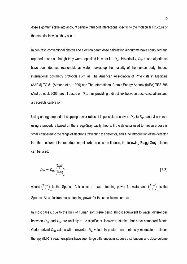
Using energy dependant stopping power ratios, it is possible to convert 𝐷𝑤 to 𝐷𝑚 (and vice versa)

using a procedure based on the Bragg-Gray cavity theory. If the detector used to measure dose is

small compared to the range of electrons traversing the detector, and if the introduction of the detector

into the medium of interest does not disturb the electron fluence, the following Bragg-Gray relation

can be used:

𝐷𝑤 = 𝐷𝑚

(𝑆𝑐𝑜𝑙

𝜌)

𝑤

(𝑆𝑐𝑜𝑙

𝜌)

𝑚

[2.2]

where (𝑆𝑐𝑜𝑙

𝜌)

𝑤is the Spencer-Attix electron mass stopping power for water and (

𝑆𝑐𝑜𝑙

𝜌)

𝑚is the

Spencer-Attix electron mass stopping power for the specific medium, 𝑚.

In most cases, due to the bulk of human soft tissue being almost equivalent to water, differences

between 𝐷𝑚 and 𝐷𝑤 are unlikely to be significant. However, studies that have compared Monte

Carlo-derived 𝐷𝑚 values with converted 𝐷𝑤 values in photon beam intensity modulated radiation

therapy (IMRT) treatment plans have seen large differences in isodose distributions and dose-volume

11

histograms (DVHs) when examining sites with high density contrasts. Dogan, Siebers & Keall (2006)

have shown DVH differences of up to 5.8% for head and neck treatment sites and 8% in prostate

cases (where hard bone femoral heads are present). Such significant variation between the 𝐷𝑚 and

converted 𝐷𝑤 values has led many to ask whether doses should be prescribed and reported in terms

of 𝐷𝑚 or 𝐷𝑤 (Liu & Keall 2002; Ma & Li 2011).

While there is a gradual shift to Monte Carlo-based treatment planning systems and hence 𝐷𝑚 based

data, the huge wealth of historical radiotherapy data, including toxicity information and clinical

outcome, is based on 𝐷𝑤 prescriptions. Therefore, it is important that any shift in clinical practice

toward a 𝐷𝑚-based system be built on a sound understanding of the dosimetric and clinical

differences between 𝐷𝑚 and 𝐷𝑤 .

2.1.5 The Elekta Monaco® eMC algorithm

The Elekta Monaco® eMC algorithm consists of two main components: an electron beam phase

space engine and a dose calculation engine.

The phase space engine is a model of the transport of the electron beam through the linac treatment

head, designed to reduce calculation times. The phase space is divided into two key parts as shown

in Figure 2.1. The source phase space starts upstream of the uppermost collimating component. It is

propagated through the treatment head to the exit phase space plane, located at the lowermost

collimating element i.e. immediately in front of the applicator insert. This interface defines the start of

the dose calculation engine (Elekta 2014).

For fixed collimator set-ups, the in-patient dose calculation starts by sampling from a parameterised

version of the exit phase space, thereby eliminating the need to perform the beam transport through

12

the treatment head for each dose calculation. For example, in the case of fixed applicators (with pre-

set jaw positions) as are used at MNCCI, the source phase space is pre-propagated to the exit phase

space plane. For non-fixed collimation set ups, the dose calculation samples directly from the source

phase space.

Figure 2.1: Electron beam transport from the source phase space to the exit phase space plane

(reproduced from Elekta (2014)).

Modelling of radiation transport through the patient and calculating the dose deposition is performed

in the dose calculation engine, which uses the VMC++ Monte Carlo algorithm (Kawrakow & Fippel

2000). This algorithm is considered a Class II algorithm, a classification used to describe the way it

samples electron energy losses. In Class II algorithms, the generation of secondary electrons directly

affects the energy loss and angular deviations of the primary electrons, providing a simulation that is

close to reality (Reynaert et al. 2007). To reduce calculation times, the dose calculation engine uses

13

the Condensed History approximation (Berger 1963) and a technique called Simultaneous Transport

of Particle Steps (STOPS) whereby particles of the same energy form a “particle set” and are

transported simultaneously.

In the Elekta Monaco® eMC algorithm, the patient anatomy is represented by a 3D matrix of relative

electron density (RED) data. The properties in each voxel within this matrix are derived from CT

numbers (measured in Hounsfield Units) obtained from a series of CT sectional images of the patient

or phantom. A user-defined CT-to-RED conversion table is then used to determine the RED within

each voxel. The resulting 3D RED matrix is passed to the dose calculation engine.

The dose calculation engine assigns a tissue type or element to each voxel, based on its RED and

the 12 individual composition bins as shown in Table 2.1. It is not clear from available Elekta

documentation how interpolation of tissue type as a function of RED is performed. Tissue types are

defined using the elemental compositions as defined in The International Commission on Radiation

Units and Measurements (ICRU) Report 44 (White et al. 1989) and The International Commission on

Radiological Protection (ICRP) Report 23 (Snyder et al. 1975). For cases where the RED is greater

than 2.46, the material is assumed to be elemental iron.

14

Composition RED

Air 0.00109

Lung (ICRU 44) 0.50

Adipose (ICRU 44) 0.95

Muscle (ICRU 44) 1.04

Cartilage (ICRP) 1.08

2/3 Cartilage, 1/3 Bone 1.29

1/3 Cartilage, 2/3 Bone 1.52

Bone (ICRP 23) 1.95

½ Bone, ½ Aluminium 2.15

Aluminium 2.46

Iron > 2.46

Water 1.00

Table 2.1: Compositions used by the Elekta Monaco® eMC dose calculation engine based on the

RED of individual voxels (Elekta 2014).

The Elekta Monaco® eMC dose calculation engine has three dose calculation options available, which

are described below.

• 𝐷𝑚: the transport of particles through the patient is modelled using interaction cross sections

of the medium. The absorbed dose in each voxel is calculated using the stopping power of

the medium in that voxel.

• 𝐷𝑤: the transport of particles through the patient is still carried out using interaction cross

sections for the medium. However, the Elekta Monaco® eMC algorithm scores the dose

deposition using the stopping power ratio of water-to-medium, as per equation 2.2.

15

• Dose forced to water (DFw): in this case, the entire patient is represented as pure water (i.e.

the RED is equal to 1.00). The Elekta Monaco® eMC algorithm models the transport of

particles through the patient and scores the dose deposition in terms of water. Therefore,

both the interaction cross sections and the stopping power are for water.

The dose calculation options used in this research project are primarily DFw (in Chapter 3) and 𝐷𝑚

(in Chapter 4 and Chapter 5).

2.2 Acute toxicity

To date, little work has been carried out to quantify the clinical effect on patients from changing to a

Monte Carlo 𝐷𝑚-based treatment planning approach in the case of clinical electron beams. Acute

toxicity is one radiobiological measure that could be used to judge the effect of such a change. Given

the observation at MNCCI that more MU, on average, were delivered in patient treatments when

using the calculated 𝐷𝑚-based MU, acute toxicity is a logical outcome to assess.

In radiotherapy, toxicity refers to any side effects that occur as a result of radiation treatment.

Generally, side effects that occur within 90 days of irradiation are considered acute, while those that

occur after 90 days are referred to as late. Acute toxicity results from the death of a large number of

cells and may occur within a few days or weeks after irradiation. For these cells, damage is quickly

repaired because of the rapid proliferation of stem cells and so is usually completely reversible. Acute

effects occur mainly in tissue with rapid cell turnover such as the skin, gastrointestinal epithelium and

the hematopoietic system.

Standardised classification schemes to quantify acute toxicity have been devised, which take into

account the frequency of assessment required to safely assess and manage acute reactions, and

16

the grading system to be used. Examples of classification schemes include RTOG/EORTC (Cox,

Stetz & Pajak 1995) and CTCAE (U.S Department of Health and Human Services 2009). These

systems are used on a regular basis by treatment staff within a radiotherapy department to assess

the severity of patient acute toxicity during and after treatment. These assessments are then stored

within the patient record.

Acute skin toxicity is particularly common in radiotherapy treatment – it can range from low-level

symptoms such as dull erythema and dry desquamation to severe disorders including ulceration,

haemorrhage and necrosis. In the case of these severe skin reactions (i.e. Grade 3 and Grade 4),

permanent skin changes may result. Furthermore, associated pain and discomfort may lead to

temporary or permanent cessation of radiation treatment. Therefore, it is vitally important that acute

toxicity is minimised, assessed regularly and managed proactively by treatment staff.

Studies in this field are often used to identify predictive factors (clinical or dosimetric) of radiation-

induced toxicity for a particular treatment type. For example, a study investigating radiation-induced

skin toxicity in breast cancer patients found that dose inhomogeneities greater than 107% of the

prescribed dose were the most important predictor of Grade 2 and Grade 3 acute skin reactions

(Tortorelli et al. 2013).

Alternatively, studies may be performed that compare the severity of acute toxicity across two cohorts

of patients who underwent different treatment methodologies. For example, an acute toxicity cohort

comparison was performed for 3D conformal proton therapy versus IMRT for head and neck cancer

patients (McDonald et al. 2016). The study found that proton therapy was associated with reduced

rates of gastrostomy tube dependence and pain. In another example, a cohort study compared the

severity of acute skin toxicity in breast cancer patients: one cohort was treated with image guided

radiation therapy (IGRT) while the other cohort was treated with IMRT combined with an electronic

17

portal imaging device (EPID). The study found the severity of acute radiation dermatitis was

significantly lower for patients in the IGRT cohort (Lin et al. 2018).

This literature review identified no studies that investigated differences in acute skin toxicity for

electron patients treated with 𝐷𝑤-based MU compared with patients treated with Monte Carlo-derived

𝐷𝑚-based MU. Given the differences reported between Monte Carlo-derived MU calculations and

MU calculations based on water measurements, particularly in areas containing significant tissue

inhomogeneity, a clinically observable difference in skin reaction between the two methodologies is

plausible. This gap in the literature provides a unique opportunity to better assess the clinical effect

on the patient due to this change in clinical practice.

18

3 Validation of dose to water in the Elekta Monaco® eMC

algorithm in a homogeneous plastic water phantom

To answer research question 1, a two-step approach is required. This chapter describes the first step,

whereby a simple scenario is tested in the Elekta Monaco® eMC algorithm in terms of 𝐷𝑤.

3.1 Introduction

A comparison was performed between dose measured with an ionisation chamber and dose

calculated by the Elekta Monaco® eMC algorithm in a homogeneous plastic water phantom. The

purpose of this comparison was to validate the ability of the Elekta Monaco® eMC algorithm to

accurately predict the 𝐷𝑤 in a simple scenario, thereby building confidence so that studies in more

complex scenarios could be addressed (these are described in Chapter 4).

In addition, these measurements allowed a dosimetry calculation system to be developed for a

cylindrical ionisation chamber, so that absorbed dose to water traceable to The Australian Radiation

Protection and Nuclear Safety Agency (ARPANSA) could be accurately determined from ionisation

measurements in electron beams. If the results validated that the cylindrical ionisation chamber was

able to accurately measure the 𝐷𝑤 in electron beams, it was thought that the dosimetry calculation

system could be expanded to 𝐷𝑚 (i.e. measurement of 𝐷𝑤 corrected to 𝐷𝑚) in Chapter 4.

19

3.2 Materials and methods

3.2.1 Radiation detector

The radiation detector used for all measurements was an IBA CC04 cylindrical ionisation chamber

(serial number 14571). This ionisation chamber has a relatively small cavity volume of 0.04 cm3, with

a cavity length and radius of 3.6 mm and 2 mm respectively.

Ideally, a plane parallel ionisation chamber would have been used. Plane parallel chambers are

considered the gold standard in electron beam dosimetry due to their physical characteristics (e.g.

disc-type shape and guard rings, which minimise scatter perturbation effects) that make them ideal

in electron beams. However, the CC04 cylindrical ionisation chamber was selected based on its

ability to fit within the various phantoms used in the intended full scope of this research project.

To ensure that the CC04 cylindrical ionisation chamber could accurately measure dose in electron

beams, percentage depth dose (PDD) measurements using the CC04 cylindrical ionisation chamber

were compared with those using a PTW Roos® plane parallel ionisation chamber (sensitive volume:

0.35 cm3, sensitive volume radius: 7.8 mm, sensitive volume depth: 2 mm). Percentage depth

ionisation (PDI) scans (10 cm x 10 cm applicator, 100 cm SSD, gantry and collimator at 0°) for each

electron beam energy were performed in a full-scatter water tank (IBA Blue Phantom) using the CC04

ionisation chamber and Roos® chamber as the field detector and a CC13 ionisation chamber as the

reference detector. Conversion to PDD was carried out within IBA OmniPro software according to

the IAEA TRS-398 dosimetry protocol.

The CC04 ionisation chamber was cross calibrated for use in electron beams according to IAEA TRS-

398, using the MNCCI secondary standard ionisation chamber (NE 2571; serial number 3481). The

20

cross calibration was performed using a cross calibration beam quality, 𝑄𝑐𝑟𝑜𝑠𝑠, of 15 MeV (the

highest electron energy available in the local department). During the cross calibration, values for the

polarity correction factor, 𝑘𝑝𝑜𝑙, and the recombination correction factor, 𝑘𝑠, were determined. To

validate the cross calibration factor obtained, an absorbed dose determination according to the IAEA

TRS-398 protocol was carried out for all electron beams using the CC04 ionisation chamber, followed

by the same measurements using a calibrated Roos® plane parallel chamber.

3.2.2 Homogeneous plastic water phantom

The phantom used for all measurements was the IBA IMRT phantom, which is shown in Figure 3.1.

This phantom is approximately torso shaped, is composed of RW3 plastic material (composition: 98%

polystyrol + 2% Ti02; nominal density: 1.045 g/cm3) and has a modular design allowing ionisation

chamber placement at various depths within the phantom geometry.

Figure 3.1: A transverse slice through the IBA IMRT phantom used for depth-dose measurements

with the CC04 cylindrical ionisation chamber. The particular slice shown is positioned at the centre

of the ionisation chamber slot (shown by the red contour).

21

3.2.3 Electrometer

The electrometer used for all measurements was a Scandatronix Wellhofer Dose 1 (serial number

16717) with a bias voltage of +300 V applied. A 60-second background reading was taken and

subtracted from all subsequent measurements. The electrometer correction factor, 𝑘𝑒𝑙𝑒𝑐, used for

absorbed dose determination was obtained from the relevant ARPANSA calibration certificate.

3.2.4 Electron beam energies

Electron beam energies available for use in the local department are 6 MeV, 9 MeV, 12 MeV and 15

MeV – all electron beams were investigated as part of this research project.

3.2.5 Creation of treatment plans

The IMRT phantom was scanned using a 64-slice Siemens SOMATOM Confidence CT scanner.

Data was exported to the Monaco® TPS where a series of electron plans were created and dose

calculations performed. The steps undertaken to obtain the treatment plans in the Elekta Monaco®

eMC algorithm are outlined below.

• The phantom was placed on the CT couch and scanned using one of the standard clinical

protocols used in the department.

• The CT dataset was imported into the Monaco® TPS via DICOM-RT.

• The external boundary of the CT dataset was contoured.

• Electron plans were created for each energy, using a 10 cm x 10 cm applicator, at 100 cm

SSD and gantry and collimator settings at 0°.

22

• Dose calculations were performed in the Elekta Monaco® eMC algorithm by delivering 100

MU, using the DFw dose deposition option. To determine the optimal calculation settings,

calculations were performed using two scenarios: 1,000,000 histories with a grid cell size of

0.1 cm (named “detailed” plans), and 750,000 histories with a grid cell size of 0.2 cm (named

“standard” plans).

• Sagittal dose planes from each of the dose calculations were exported from the Monaco®

TPS and subsequently imported into Microsoft Excel as text files.

• Point doses were extracted from the Monaco® TPS dose plane data in Microsoft Excel at

the ionisation chamber measurement points that would be used within the IMRT phantom.

3.2.6 Phantom set-up and measurements

The phantom was set up to the isocentre on the treatment couch, at 100 cm SSD and with the gantry

and collimator set to 0°. Charge measurements were taken with the ionisation chamber at various

depths within the IMRT phantom. The measurement depths were selected to obtain adequate data

coverage over the area from approximately R100 to R50 and, therefore, were dependent on the

electron energy (where R100 is the depth in water at which the absorbed dose is maximum and R50 is

the depth in water at which the absorbed dose is 50% of its maximum value). The effective point of

measurement of the ionisation chamber was accounted for when placing the chamber at each

measurement location. A minimum of 10 cm of backscatter material and 5 cm of lateral side-scatter

material within the phantom was present around the chamber for all measurements.

Three 100 MU exposures were delivered at each measurement depth and for each energy. For each

of the three exposures, a charge reading was taken with the results averaged (𝑀1).

23

Temperature and pressure readings were taken at regular intervals during data collection in order to

calculate the temperature and pressure correction factor, 𝑘𝑡𝑝, necessary for absorbed dose

determination.

3.2.7 Dose calculation formalism (𝑫𝒘)

The absorbed dose to water, 𝐷𝑤,𝑄, at the user beam quality 𝑄 was determined from ionisation

measurements according to the IAEA TRS-398 protocol as follows:

𝐷𝑤,𝑄 = 𝑀𝑄 𝑁𝐷,𝑤,𝑄𝑐𝑟𝑜𝑠𝑠 𝑘𝑄,𝑄𝑐𝑟𝑜𝑠𝑠 [3.1]

where 𝑁𝐷,𝑤,𝑄𝑐𝑟𝑜𝑠𝑠 is the chamber calibration factor in terms of absorbed dose to water at the cross

calibration beam quality, 𝑘𝑄,𝑄𝑐𝑟𝑜𝑠𝑠 is the beam quality correction factor to account for the difference

between the response of the ionisation chamber in the user beam quality and the cross calibration

beam quality and 𝑀𝑄 is the reading of the ionisation chamber at the user beam quality, corrected for

influencing quantities as given by:

𝑀𝑄 = 𝑀1 𝑘𝑡𝑝 𝑘𝑠 𝑘𝑝𝑜𝑙 𝑘𝑒𝑙𝑒𝑐 [3.2]

According to IAEA TRS-398 Section 7.7 (“Measurements under non-reference conditions”),

measured depth-ionisation readings must be converted to depth-dose by multiplying them by the

water-to-air Spencer-Attix stopping power ratio, 𝑠𝑤,𝑎𝑖𝑟, for the electron beam quality specifier R50 at

the depth of interest. Values for the stopping power ratios were obtained from IAEA TRS-398 Table

7.V by interpolation between table entries. To obtain the stopping power ratio correction factor that

was applied to the ionisation readings, the stopping power ratio at the depth of interest was

normalised to the stopping power ratio at the reference depth, 𝑧𝑟𝑒𝑓. The rationale for this step is

shown in the mathematical derivation below.

24

From equation 3.1, at 𝑧𝑟𝑒𝑓:

𝐷𝑤,𝑄(𝑧𝑟𝑒𝑓) = 𝑀𝑄 (𝑧𝑟𝑒𝑓) 𝑁𝐷,𝑤,𝑄𝑐𝑟𝑜𝑠𝑠 𝑘𝑄,𝑄𝑐𝑟𝑜𝑠𝑠 [3.3]

where:

𝑘𝑄,𝑄𝑐𝑟𝑜𝑠𝑠 =(𝑠𝑤,𝑎𝑖𝑟)

𝑄 𝑧𝑟𝑒𝑓 (𝑤𝑎𝑖𝑟)𝑄 𝑧𝑟𝑒𝑓

𝑝𝑄 𝑧𝑟𝑒𝑓

(𝑠𝑤,𝑎𝑖𝑟)𝑄𝑐𝑟𝑜𝑠𝑠

(𝑤𝑎𝑖𝑟)𝑄𝑐𝑟𝑜𝑠𝑠 𝑝𝑄𝑐𝑟𝑜𝑠𝑠

[3.4]

where 𝑤𝑎𝑖𝑟 is the mean energy expended in air per ion pair formed at the particular beam quality 𝑄

or 𝑄𝑐𝑟𝑜𝑠𝑠 and 𝑝 is the overall perturbation factor for the ionisation chamber at the particular beam

quality 𝑄 or 𝑄𝑐𝑟𝑜𝑠𝑠.

At any measurement depth, 𝑧:

𝐷𝑤,𝑄(𝑧) = 𝑀𝑄 (𝑧) 𝑁𝐷,𝑤,𝑄𝑐𝑟𝑜𝑠𝑠 𝑘𝑄𝑧,𝑄𝑐𝑟𝑜𝑠𝑠 [3.5]

where:

𝑘𝑄𝑧,𝑄𝑐𝑟𝑜𝑠𝑠 =𝑘𝑄𝑧

𝑘𝑄𝑧𝑟𝑒𝑓

×𝑘𝑄𝑧𝑟𝑒𝑓

𝑘𝑄𝑐𝑟𝑜𝑠𝑠

[3.6]

From equation 3.6:


𝑘𝑄𝑐𝑟𝑜𝑠𝑠

= 𝑘𝑄,𝑄𝑐𝑟𝑜𝑠𝑠 [3.7]

and:

𝑘𝑄𝑧


=(𝑠𝑤,𝑎𝑖𝑟)

𝑄𝑧 (𝑤𝑎𝑖𝑟)𝑄𝑧 𝑝𝑄𝑧

(𝑠𝑤,𝑎𝑖𝑟)𝑄 𝑧𝑟𝑒𝑓

(𝑤𝑎𝑖𝑟)𝑄 𝑧𝑟𝑒𝑓 𝑝𝑄 𝑧𝑟𝑒𝑓

[3.8]

25

Therefore,

𝑘𝑄𝑧,𝑄𝑐𝑟𝑜𝑠𝑠 = ((𝑠𝑤,𝑎𝑖𝑟)

𝑄𝑧 (𝑤𝑎𝑖𝑟)𝑄𝑧 𝑝𝑄𝑧


(𝑤𝑎𝑖𝑟)𝑄 𝑧𝑟𝑒𝑓 𝑝𝑄 𝑧𝑟𝑒𝑓

) × 𝑘𝑄,𝑄𝑐𝑟𝑜𝑠𝑠 [3.9]

Substituting equation 3.9 and assuming 𝑤𝑎𝑖𝑟 and 𝑝𝑄 are constants, equation 3.5 becomes:

𝐷𝑤,𝑄(𝑧) = 𝑀𝑄 (𝑧) 𝑁𝐷,𝑤,𝑄𝑐𝑟𝑜𝑠𝑠 𝑘𝑄,𝑄𝑐𝑟𝑜𝑠𝑠

(𝑠𝑤,𝑎𝑖𝑟)𝑄𝑧


[3.10]

3.2.8 Electron dosimetry considerations in plastic phantoms

When depth-dose measurements are carried out in plastic, the depths must be scaled to give the

equivalent depths in water (i.e. depth-scaling), while the dosimeter readings must be scaled to give

the equivalent reading in water (i.e. fluence-scaling). Both depth-scaling and fluence-scaling of all

depth-dose measurements were carried out using the methodology given in Section 7.8 of IAEA TRS-

398. The methodology is summarised here for reference.

Each measurement depth in plastic, 𝑧𝑝𝑙, was scaled to give the equivalent depth in water, 𝑧𝑤, using:

𝑧𝑤 = 𝑧𝑝𝑙 𝑐𝑝𝑙 [3.11]

where 𝑐𝑝𝑙 is known as the depth-scaling factor, and both 𝑧𝑤 and 𝑧𝑝𝑙 are expressed in units of g cm2.

The depth in plastic, 𝑧𝑝𝑙, was determined by multiplying the physical measurement depth (in cm) by

the physical density of the plastic, 𝜌𝑝𝑙. As per the recommendation in IAEA TRS-398, the physical

density was measured for the specific batch of RW3 plastic in the IMRT phantom. Measurement of

the plastic dimensions was made using a micrometer while the mass was measured using high

precision scales.

26

Values of 𝑐𝑝𝑙 for certain plastic types are provided in Table 7.VI of IAEA TRS-398 and are reproduced

in Table 3.1. As RW3 plastic is not included in this table, it was necessary to obtain a customised

depth-scaling factor.

Plastic phantom 𝒄𝒑𝒍 𝒉𝒑𝒍 𝝆𝒑𝒍 (g/cm3)

Solid water® (WT1) 0.949 1.011 1.020

Solid water® (RMI-457) 0.949 1.008 1.030

Plastic water 0.982 0.998 1.013

Virtual water 0.946 Not available 1.030

PMMA 0.941 1.009 1.190

Clear polystyrene 0.922 1.026 1.060

White polystyrene 0.922 1.019 1.060

A-150 0.948 Not available 1.127

Table 3.1: Values of the depth-scaling factor, fluence-scaling factor (ℎ𝑝𝑙) and physical density for

various plastic types, reproduced from Table 7.VI of IAEA TRS-398 (Andreo et al. 2006).

To determine the customised depth-scaling factor, depth-dose measurements were carried out using

the CC04 ionisation chamber in a water tank, followed by the same measurements in the IMRT

phantom. For the water tank measurements, PDI scans (10 cm x 10 cm applicator, 100 cm SSD,

gantry and collimator at 0°) for each electron beam energy were obtained using the CC04 ionisation

chamber as the field detector and a CC13 ionisation chamber as the reference detector. Conversion

to PDD was carried out within IBA OmniPro software according to the IAEA TRS-398 protocol.

PDI measurements (10 cm x 10 cm applicator, 100 cm SSD, gantry and collimator at 0°) for each

electron energy were then performed in the IMRT phantom using the CC04 ionisation chamber.

100 MU were delivered, with three charge readings taken at each depth and for each energy, with

the result averaged. Conversion to PDD was carried out by manually applying the appropriate

Spencer-Attix stopping power ratio from IAEA TRS-398.

27

An overall depth-scaling factor, referred to here as “ODSF”, was determined by applying various

factors to the IMRT phantom measurement depths until the root mean square error between the

PDDs measured in water and the PDDs measured in the IMRT phantom was minimised. From

determination of the ODSF value and the measured physical density of the plastic, the depth-scaling

factor, 𝑐𝑝𝑙, could be calculated using:

𝑐𝑝𝑙 = 𝑂𝐷𝑆𝐹

𝜌𝑝𝑙 [3.12]

In addition to depth-scaling, the dosimeter reading at each depth in plastic, 𝑀𝑄,𝑝𝑙, must also be

scaled by the fluence-scaling factor, ℎ𝑝𝑙 , to obtain the equivalent reading in water, 𝑀𝑄, using:

𝑀𝑄 = 𝑀𝑄,𝑝𝑙 ℎ𝑝𝑙 [3.13]

As per the methodology given in IAEA TRS-398, for depths beyond the reference depth in plastic,

𝑧𝑟𝑒𝑓,𝑝𝑙, the determined value of ℎ𝑝𝑙 at 𝑧𝑟𝑒𝑓,𝑝𝑙 is used. For shallower depths, this value of ℎ𝑝𝑙 is

decreased linearly to a value of unity at zero depth.

Similar to the depth-scaling factor, no ℎ𝑝𝑙 value for RW3 plastic is available in IAEA TRS-398. The

ℎ𝑝𝑙 value used for fluence-scaling of charge measurements was obtained from Table 7.VI of IAEA

TRS-398 (reproduced in Table 3.1) for the plastic type that provided the closest match of the 𝑐𝑝𝑙 and

𝜌𝑝𝑙 values determined for the IMRT phantom. The uncertainty associated with this assumption for

the ℎ𝑝𝑙 value is ± 0.3%.

28

3.3 Results

3.3.1 Validation of the CC04 ionisation chamber for use in electron beams

PDD measurements performed in water using the CC04 ionisation chamber and the Roos® plane

parallel chamber for all electron energies are shown in Figure 3.2. At the depths of clinical significance

(i.e. from approximately R100 to R80 where R80 is the depth in water at which the absorbed dose is

80% of its maximum value), the maximum discrepancy between the measurements performed with

the CC04 ionisation chamber and the Roos® plane parallel chamber was ± 1.5%. This level of

agreement was deemed to be acceptable and validates that the CC04 ionisation chamber is an

acceptable detector for the accurate measurement of percent depth dose in the electron beams under

investigation in this research project.

Figure 3.2: PDD measurements using the Roos® plane parallel chamber and the CC04 ionisation

chamber in water for all electron beam energies. The Elekta Monaco® eMC DFw calculated data are

also shown for reference.

29

The absorbed dose determination results from both the CC04 ionisation chamber and the Roos®

plane parallel chamber were within 1% of nominal (i.e. 1 cGy/MU) and the CC04 ionisation chamber

results were within 1% of the Roos® plane parallel chamber results. This level of agreement was

deemed to be acceptable and validates that the CC04 ionisation chamber is an acceptable detector

for the accurate measurement of absorbed dose in the electron beams under investigation in this

research project.

3.3.2 Optimal dose calculation parameters and export format

An analysis was performed to determine which data export format (i.e. interest point dose or dose

plane) and which Elekta Monaco® eMC calculation parameters (i.e. standard or detailed) provided

the best level of agreement between the calculated and measured datasets. The exported dose plane

data (with point doses subsequently extracted from it) and the detailed calculations provided the best

agreement with the measured data. This analysis was performed for 6 MeV and 15 MeV beams only,

but it is reasonable to assume that similar results would be obtained for the 9 MeV and 12 MeV

beams. Therefore, all Elekta Monaco® eMC data used in this research project are calculated in

detailed mode and extracted from exported dose planes.

3.3.3 Determination of the physical density, depth-scaling and fluence-scaling factors

The physical density of the IMRT phantom plastic, 𝜌𝑝𝑙, was measured as 1.043 g/cm3 ± 0.4%, which

agrees (within the experimental uncertainty) with the manufacturer stated value of 1.045 g/cm3.

The ODSF value that minimised the root mean square error between PDD data measured in water

and PDD data measured in the IMRT phantom was 0.98 ± 1% for all electron energies. Figure 3.3

shows this PDD data obtained using the CC04 ionisation chamber in water and in the IMRT phantom

30

for all energies, with the measurement depths in the plastic multiplied by the optimal ODSF value of

0.98.

Using the measured 𝜌𝑝𝑙 and the ODSF value obtained, the value for the depth-scaling factor, 𝑐𝑝𝑙,

was determined to be 0.94 ± 1.1% using equation 3.12.

Figure 3.3: PDD measurements using the CC04 ionisation chamber in water and in the IMRT

phantom for all electron energies. The customised ODSF of 0.98 has been applied to the physical

measurement depths in the IMRT phantom.

As Table 3.1 shows, the plastic type that provided the closest match to both the 𝑐𝑝𝑙 and 𝜌𝑝𝑙 values

obtained for RW3 plastic was “Solid water® (RMI-457)”. Therefore, the ℎ𝑝𝑙 value used in subsequent

dose calculations was 1.008 ± 0.4% as for Solid water® (RMI-457).

31

Table 3.2 summarises the physical density and scaling factors used in subsequent dose calculations

using the IMRT phantom.

Plastic phantom 𝒄𝒑𝒍 𝒉𝒑𝒍 𝝆𝒑𝒍 (g/cm3)

IBA IMRT (RW3 plastic) 0.94 ± 1.1% 1.008 ± 0.4% 1 1.043 ± 0.4%

Table 3.2: Values of the depth-scaling factor, fluence-scaling factor and physical density for the IBA

IMRT phantom (RW3 plastic). 1The fluence-scaling factor was taken from IAEA TRS-398 as a “best

match” to Solid water® (RMI-457).

3.3.4 Comparison between Elekta Monaco® eMC dose calculations and measured 𝑫𝒘 in the

homogeneous plastic water phantom

The final results comparing the level of agreement between the Elekta Monaco® eMC DFw dose

calculations and the depth-dose data measured in the IMRT phantom are shown in Figure 3.4, while

Table 3.3 quantifies the differences observed. The physical measurement depths in the IMRT

phantom have been scaled using the customised ODSF of 0.98.

32

Figure 3.4: Comparisons of Elekta Monaco® eMC DFw dose calculations and the measured 𝐷𝑤

(using the CC04 ionisation chamber) in the IMRT phantom for all electron beams. The customised

ODSF of 0.98 has been applied to the physical measurement depths in the IMRT phantom.

Table 3.3: Differences between the Elekta Monaco® eMC DFw dose calculations and the measured

𝐷𝑤 in the IMRT phantom for all electron beams (normalised to the maximum DFw calculated dose).

Difference values exceeding 3% are highlighted in red.

Differences between the Elekta Monaco® eMC DFw dose calculations and the measured 𝐷𝑤 data

are within ± 3% for the 9 MeV, 12 MeV and 15 MeV beams, while larger discrepancies of up to 4.1%

are observed for the 6 MeV beam.

Physical

measurement

depth (cm)

Difference

calculated vs.

measured

Physical

measurement

depth (cm)

Difference

calculated vs.

measured

Physical

measurement

depth (cm)

Difference

calculated vs.

measured

Physical

measurement

depth (cm)

Difference

calculated vs.

measured

1 0.9% 1 -0.6% 1 1.6% 2 2.5%

1.3 1.4% 1.5 0.2% 2 -1.7% 2.6 1.9%

1.5 1.9% 2 -0.7% 3 -1.2% 3.5 1.2%

1.8 2.9% 2.5 0.5% 4 -1.7% 4.5 -1.8%

2 4.1% 3 1.0% 5 0.7% 5 -1.7%

2.5 2.1% 3.5 2.0% 6 -1.0%

4 1.9%

6 MeV 9 MeV 12 MeV 15 MeV

33

3.4 Discussion

The comparison of 𝐷𝑤 measured in a simple, homogeneous plastic water phantom with the Elekta

Monaco® eMC DFw calculated data is within ± 3% for the 9 MeV, 12 MeV and 15 MeV electron

beams. The relative standard uncertainty in the measured 𝐷𝑤 data is at least 2.4%. This estimate is

based on uncertainties quoted in IAEA TRS-398 at the reference depth in water for a cylindrical

ionisation chamber used in electron beams (which has been calibrated in 60Co). It also accounts for

the additional uncertainty due to the cross calibration of the secondary standard NE 2571 ionisation

chamber with the CC04 ionisation chamber and subsequent use of the CC04 ionisation chamber for

depth-dose measurements. The uncertainty is likely to be higher at depths away from the reference

depth, and due to the measurements being performed in plastic. The uncertainty in the Elekta

Monaco® eMC dose calculations could not be quantified due to the random number generator seed

remaining the same for repeated calculations.

The AAPM recommend a tolerance level of 3%/3 mm for basic TPS validation in the case of electron

dose calculation algorithms (Smilowitz et al. 2015). Based on these recommendations, the dose

comparison results obtained for the 9 MeV, 12 MeV and 15 MeV electron beams validate that the

Elekta Monaco® eMC algorithm is able to accurately predict the dose in a simple scenario for these

beam energies.

However, there is a larger discrepancy (up to 4.1%) observed for the 6 MeV data. It is likely that this

discrepancy is affected, at least in part, by the steep gradient of the 6 MeV PDD curve (i.e. 6.9%/mm

in the region of approximately R90 to R40, where R40 is the depth in water at which the absorbed

dose is 40% of its maximum value). Any small errors in the measurement depth (e.g. due to

inaccurate machining of the plastic water slabs within the IMRT phantom or increased air gaps

between the individual plastic slabs or both), will have a relatively larger effect on the 6 MeV

34

measured data, leading to a greater discrepancy with the Elekta Monaco® eMC data. Given the error

in the thickness of the plastic water slabs was 0.05 mm per slab (nominal thickness of 1 cm), at a

physical depth of 2 cm, the combined error in the slab thickness would lead to a 0.7% difference in

the PDD value.

Additionally, 𝑘𝑄,𝑄𝑖𝑛𝑡 factors (i.e. beam quality correction factors that account for the difference

between the response of the ionisation chamber in the user beam quality 𝑄 and an intermediate

beam quality 𝑄𝑖𝑛𝑡) are not available in IAEA TRS-398 for cylindrical chambers in electron beams

with a R50 less than 4 g cm2. In this case, 𝑘𝑄,𝑄𝑖𝑛𝑡 factors could only be obtained for the 12 MeV (R50

= 4.72 cm) and 15 MeV (R50 = 6 cm) beams, while factors for the 6 MeV (R50 = 2.39 cm) and 9 MeV

(R50 = 3.48 cm) beams have been extrapolated. Therefore, there is an increased level of uncertainty

in the beam quality correction factors, 𝑘𝑄,𝑄𝑐𝑟𝑜𝑠𝑠, and the measured absorbed dose data for the

6 MeV and 9 MeV beams.

There is significant variation in perturbation factors with depth in electron beams when measured

using a cylindrical ionisation chamber. IAEA TRS-398 states that perturbation factors for such

chambers have only been determined close to the reference depth. For this reason, this protocol

discourages the use of cylindrical ionisation chambers for measurements of depth-dose distributions

in electron beams. Instead, well-guarded plane parallel chambers are recommended, as they exhibit

minimal variation in the perturbation factor with depth. However, the results obtained in this research

project show that the CC04 cylindrical ionisation chamber produces an acceptable level of agreement

with a well-guarded Roos® plane parallel chamber for depth-dose measurements in all of the electron

beams under investigation.

IAEA TRS-398 states that the use of plastic phantoms is permitted in electron beams with beam

qualities of R50 less than 4 g cm2 (i.e. < 10 MeV). However, this protocol also advises that their use

35

in electron beams is strongly discouraged as large errors in the determination of absorbed dose can

result. These errors are mainly due to the uncertainty related to the scaling factors applied. By using

a customised depth-scaling factor, and measurement of the physical density of the specific plastic

batch used in the IMRT phantom, uncertainties in the absorbed dose to water when measured in

plastic have been minimised.

3.5 Conclusions

The CC04 cylindrical ionisation chamber used in this research project has been shown to accurately

measure absorbed dose to water in electron beams across the range of depths that are of clinical

interest.

The dose comparisons show that the Elekta Monaco® eMC algorithm is able to accurately predict the

dose in a homogeneous plastic water phantom, using simple beam geometries. Differences between

the DFw calculated data and the measured 𝐷𝑤 data in the IMRT phantom are within ± 3% for the

9 MeV, 12 MeV and 15 MeV beams, while slightly larger discrepancies of up to 4.1% are observed

for the 6 MeV beam.

Reasons for the poorer level of agreement observed for the 6 MeV data include dose gradient effects

and the higher uncertainty in the beam quality correction factor, 𝑘𝑄,𝑄𝑐𝑟𝑜𝑠𝑠, used for absorbed dose

to water determination.

Use of the CC04 cylindrical ionisation chamber with the application of a customised ODSF for the

specific phantom material provides a robust dosimetry system for future measurements of absorbed

dose in more complex scenarios. However, the larger discrepancies observed for the 6 MeV data

indicate that caution will be required when interpreting future results for the 6 MeV electron beam.

36

4 Validation of dose to medium in the Elekta Monaco® eMC

algorithm in tissue equivalent slab phantoms

This chapter describes the final step required to address research question 1, whereby more clinically

relevant scenarios are tested in the Elekta Monaco® eMC algorithm in terms of 𝐷𝑚.

4.1 Introduction

A comparison was performed between dose measured with the CC04 cylindrical ionisation chamber

and dose calculated by the Elekta Monaco® eMC algorithm in phantoms comprising tissue equivalent

plastic slabs of varying electron density. Simple cases (i.e. homogeneous phantoms representing a

single tissue type) as well as a more complex, clinically realistic case (i.e. an inhomogeneous

phantom comprising multiple tissue types) were investigated.

The purpose of these measurements was to assess the ability of the Elekta Monaco® eMC algorithm

to accurately predict 𝐷𝑚 in a range of commonly encountered tissue types, with the ultimate aim of

validating that the Elekta Monaco® eMC 𝐷𝑚 calculation option has acceptable accuracy for clinical

use. In order to calculate 𝐷𝑚 from measurements of ionisation in non-water equivalent media, the

dosimetry calculation system described in Chapter 3 has been expanded.

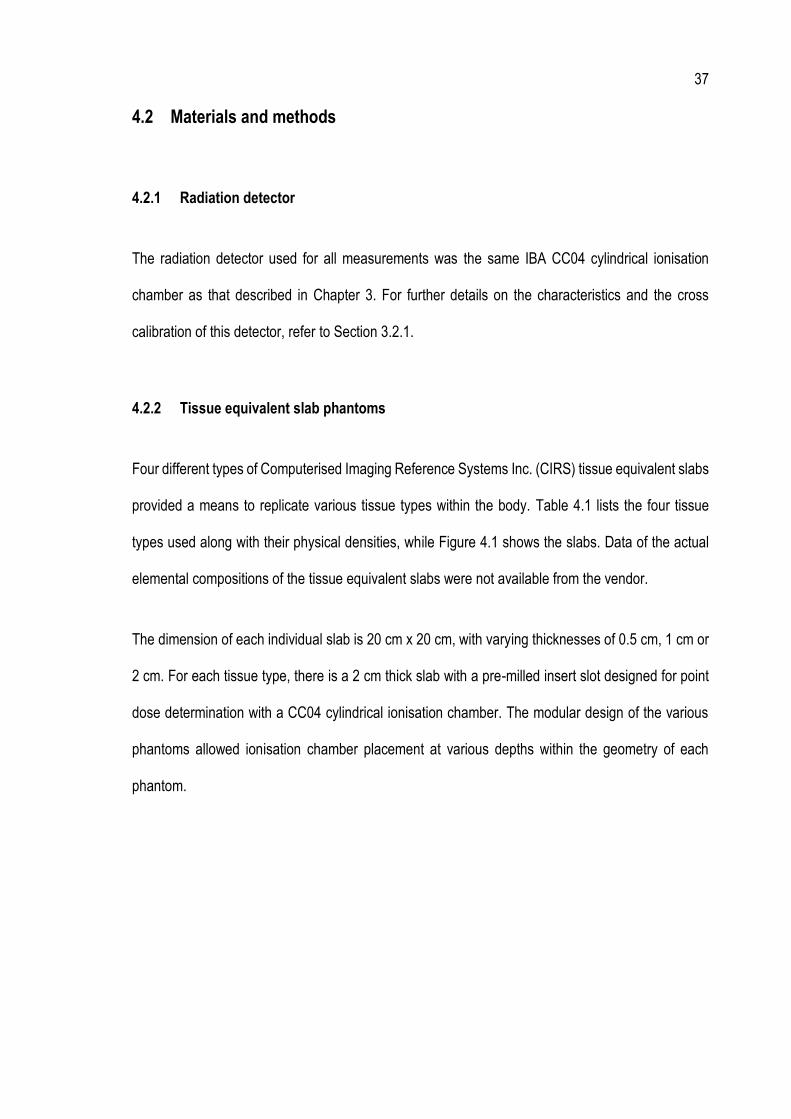
37


4.2.1 Radiation detector

The radiation detector used for all measurements was the same IBA CC04 cylindrical ionisation

chamber as that described in Chapter 3. For further details on the characteristics and the cross

calibration of this detector, refer to Section 3.2.1.

4.2.2 Tissue equivalent slab phantoms

Four different types of Computerised Imaging Reference Systems Inc. (CIRS) tissue equivalent slabs

provided a means to replicate various tissue types within the body. Table 4.1 lists the four tissue

types used along with their physical densities, while Figure 4.1 shows the slabs. Data of the actual

elemental compositions of the tissue equivalent slabs were not available from the vendor.

The dimension of each individual slab is 20 cm x 20 cm, with varying thicknesses of 0.5 cm, 1 cm or

2 cm. For each tissue type, there is a 2 cm thick slab with a pre-milled insert slot designed for point

dose determination with a CC04 cylindrical ionisation chamber. The modular design of the various

phantoms allowed ionisation chamber placement at various depths within the geometry of each

phantom.

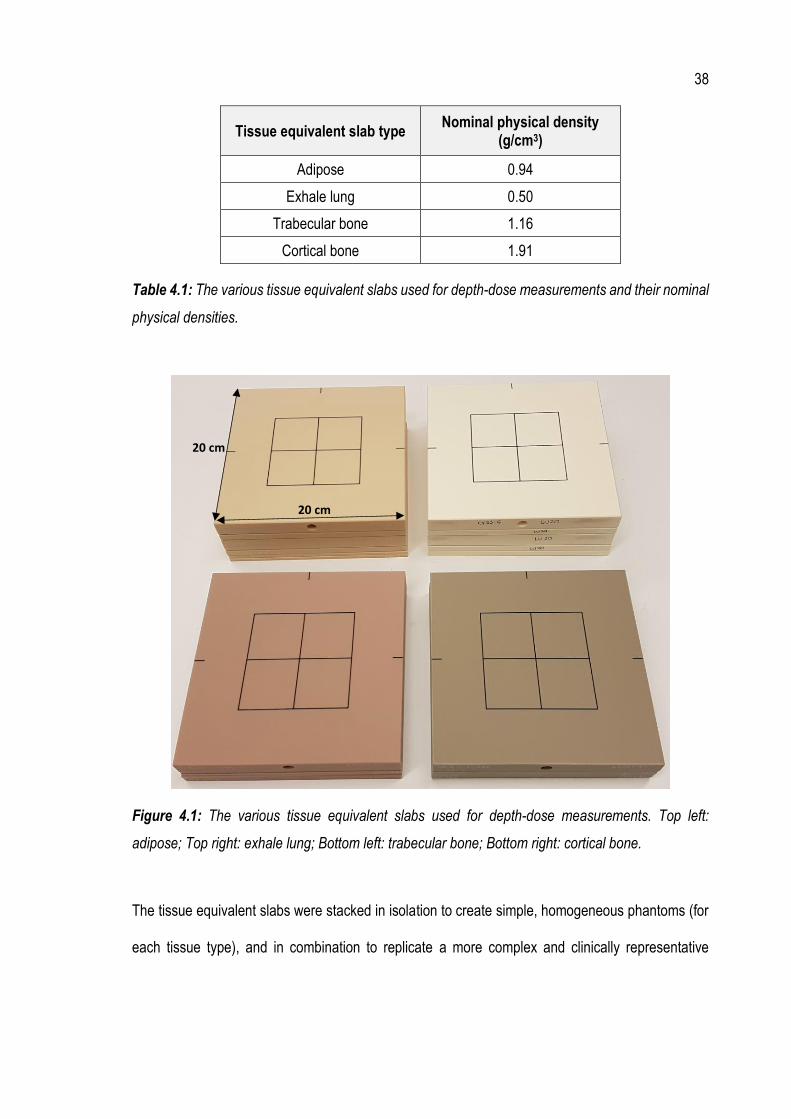
38

Tissue equivalent slab type Nominal physical density

(g/cm3)

Adipose 0.94

Exhale lung 0.50

Trabecular bone 1.16

Cortical bone 1.91

Table 4.1: The various tissue equivalent slabs used for depth-dose measurements and their nominal

physical densities.

Figure 4.1: The various tissue equivalent slabs used for depth-dose measurements. Top left:

adipose; Top right: exhale lung; Bottom left: trabecular bone; Bottom right: cortical bone.

The tissue equivalent slabs were stacked in isolation to create simple, homogeneous phantoms (for

each tissue type), and in combination to replicate a more complex and clinically representative

20 cm

20 cm

39

scenario. These two cases, referred to as “simple” and “complex”, are detailed in Section 4.2.2.1 and

4.2.2.2 respectively.

4.2.2.1 Simple: homogeneous tissue equivalent slab phantoms

A simple, homogeneous tissue equivalent slab phantom was created for each of the four tissue types.

Each phantom consisted of a stack of varying thickness tissue equivalent slabs (of the single tissue

type), with a 5 cm thick plastic water slab below to provide backscatter. An example of such a

phantom is shown for adipose in Figure 4.2.

Figure 4.2: The adipose homogeneous tissue equivalent slab phantom as used for depth-dose

measurements.

4.2.2.2 Complex: inhomogeneous tissue equivalent slab phantom

The complex, inhomogeneous tissue equivalent slab phantom was designed to replicate what would

typically be encountered in a clinical electron breast boost treatment. The phantom consisted of a

7 cm adipose

5 cm plastic water

CC04 insert slot

40

3 cm thickness of adipose, followed by a 1 cm thickness of trabecular bone, then a 4 cm thickness

of exhale lung. As for the simple phantoms, a 5 cm thick plastic water slab was placed below to

provide backscatter. The complex phantom is shown in Figure 4.3.

Figure 4.3: The complex, inhomogeneous tissue equivalent slab phantom as used for depth-dose

measurements.

4.2.3 Electrometer

As in Section 3.2.3, the electrometer used for all measurements was a Scandatronix Wellhofer Dose

1 (serial number 16717) with a bias voltage of +300 V applied. A 60-second background reading was

taken and subtracted from all subsequent measurements. The electrometer correction factor, 𝑘𝑒𝑙𝑒𝑐,

used for absorbed dose determination was obtained from the relevant ARPANSA calibration

certificate.

4 cm exhale lung

5 cm plastic water

3 cm adipose

1 cm trabecular bone

41

4.2.4 Electron beam energies

Electron beam energies available for use in the local department are 6 MeV, 9 MeV, 12 MeV and 15

MeV. All electron beams were investigated for the simple, homogeneous phantoms. However,

measurements were taken only for the 12 MeV and 15 MeV beams in the case of the complex,

inhomogeneous phantom. These two energies provided an acceptable distribution of dose with depth

in the phantom and are typical of what is used clinically for electron breast boost treatments.

4.2.5 Creation of treatment plans

The tissue equivalent slab phantoms (both simple cases and the complex case) were scanned using

a 64-slice Siemens SOMATOM Confidence CT scanner. Data was exported to the Monaco® TPS

where a series of electron plans were created and dose calculations performed. The following steps

were taken to create the treatment plans in the Elekta Monaco® eMC algorithm.

• Each phantom was placed on the CT couch and individually scanned using one of the

standard clinical protocols used in the department.

• Each CT dataset was imported into the Monaco® TPS via DICOM-RT.

• The external boundary of each CT dataset was contoured. The (empty) ion chamber insert

slot was also contoured, with the RED overridden to the average RED of the tissue material.

Initially, separate CT scans were taken with the CC04 ionisation chamber inserted within the

phantoms at each of the measurement depths. However, significant artefacts were produced

from a high density region of the chamber stem, which could not be adequately removed

using artefact reduction algorithms. Therefore, CT scans were performed without the

ionisation chamber present, and with the RED override applied for dose calculations.

42

• Electron plans were created for each energy (in the case of the simple, homogeneous tissue

equivalent slab phantoms) and for 12 MeV and 15 MeV only (in the case of the complex,

inhomogeneous tissue equivalent slab phantom), using a 10 cm x 10 cm applicator, at 100

cm SSD and gantry and collimator settings at 0°.

• Dose calculations were performed in the Elekta Monaco® eMC algorithm by delivering 100

MU, using the 𝐷𝑚 dose deposition option, with 1,000,000 histories and with a grid cell size

of 0.1 cm. In the case of the simple phantom for cortical bone, a significant artefact was

present around the empty ion chamber insert slot due to the contrast between the high

density bone and the low density air cavity. This resulted in inaccurate RED values being

assigned in the dose calculation in this artefact area. To overcome the effect of the artefact,

a RED override (equal to the average RED of the remainder of the tissue material) was

applied to the artefact area.

• Sagittal dose planes from each of the dose calculations were exported from the Monaco®

TPS and subsequently imported into Microsoft Excel as text files.

• Point doses were extracted from the Monaco® TPS dose plane data in Microsoft Excel at

the ionisation chamber measurement points that were used in each phantom, with the

effective point of measurement of the ionisation chamber (in water) taken into account.

4.2.6 Phantom set-up and measurements (for both simple and complex cases)

Each phantom was set up to the isocentre on the treatment couch, at 100 cm SSD and with the

gantry and collimator set to 0°. Charge measurements were taken with the ionisation chamber at

various depths within each of the phantoms. The effective point of measurement of the ionisation

43

chamber was accounted for through the extraction depth in the Elekta Monaco® eMC dose

calculations.

Three 100 MU exposures were delivered for each measurement depth in each phantom and for each

applicable energy. For each of the three exposures, a charge reading was taken with the results

averaged (𝑀1).

Temperature and pressure readings were taken at regular intervals during data collection, so the

temperature and pressure correction factor, 𝑘𝑡𝑝, necessary for absorbed dose determination could

be calculated.

4.2.7 Dose calculation formalism (𝑫𝒎)

The purpose of these measurements was to validate the accuracy of the dose deposited in the

medium as predicted by the Elekta Monaco® eMC algorithm. Therefore, it was necessary to calculate

the absorbed dose to medium, 𝐷𝑚,𝑄, from the charge measurements obtained in each phantom. The

steps involved in determining the measured 𝐷𝑚,𝑄 are outlined in Section 4.2.7.1 – Section 4.2.7.5.

4.2.7.1 Determination of overall depth-scaling factors and water equivalent depths

Overall depth-scaling factors, ODSFs, were determined for each tissue type and each energy using

a similar method to that described in Section 3.2.8. ODSFs were required so that water equivalent

depths for each physical measurement depth in each phantom could be determined. Water

equivalent depths were necessary in order to obtain water-to-air Spencer-Attix stopping power ratios,

𝑠𝑤,𝑎𝑖𝑟, from IAEA TRS-398.

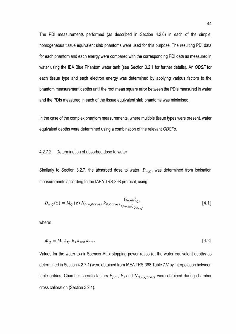
44

The PDI measurements performed (as described in Section 4.2.6) in each of the simple,

homogeneous tissue equivalent slab phantoms were used for this purpose. The resulting PDI data

for each phantom and each energy were compared with the corresponding PDI data as measured in

water using the IBA Blue Phantom water tank (see Section 3.2.1 for further details). An ODSF for

each tissue type and each electron energy was determined by applying various factors to the

phantom measurement depths until the root mean square error between the PDIs measured in water

and the PDIs measured in each of the tissue equivalent slab phantoms was minimised.

In the case of the complex phantom measurements, where multiple tissue types were present, water

equivalent depths were determined using a combination of the relevant ODSFs.

4.2.7.2 Determination of absorbed dose to water

Similarly to Section 3.2.7, the absorbed dose to water, 𝐷𝑤,𝑄, was determined from ionisation

measurements according to the IAEA TRS-398 protocol, using:

𝐷𝑤,𝑄(𝑧) = 𝑀𝑄 (𝑧) 𝑁𝐷,𝑤,𝑄𝑐𝑟𝑜𝑠𝑠 𝑘𝑄,𝑄𝑐𝑟𝑜𝑠𝑠

(𝑠𝑤,𝑎𝑖𝑟)𝑄𝑧


[4.1]

where:

𝑀𝑄 = 𝑀1 𝑘𝑡𝑝 𝑘𝑠 𝑘𝑝𝑜𝑙 𝑘𝑒𝑙𝑒𝑐 [4.2]

Values for the water-to-air Spencer-Attix stopping power ratios (at the water equivalent depths as

determined in Section 4.2.7.1) were obtained from IAEA TRS-398 Table 7.V by interpolation between

table entries. Chamber specific factors 𝑘𝑝𝑜𝑙, 𝑘𝑠 and 𝑁𝐷,𝑤,𝑄𝑐𝑟𝑜𝑠𝑠 were obtained during chamber

cross calibration (Section 3.2.1).

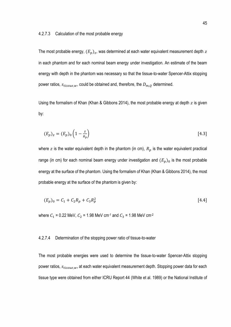
45

4.2.7.3 Calculation of the most probable energy

The most probable energy, (𝐸𝑝)𝑧, was determined at each water equivalent measurement depth 𝑧

in each phantom and for each nominal beam energy under investigation. An estimate of the beam

energy with depth in the phantom was necessary so that the tissue-to-water Spencer-Attix stopping

power ratios, 𝑠𝑡𝑖𝑠𝑠𝑢𝑒,𝑤, could be obtained and, therefore, the 𝐷𝑚,𝑄 determined.

Using the formalism of Khan (Khan & Gibbons 2014), the most probable energy at depth 𝑧 is given

by:

(𝐸𝑝)𝑧 = (𝐸𝑝)0 (1 −𝑧

𝑅𝑝) [4.3]

where 𝑧 is the water equivalent depth in the phantom (in cm), 𝑅𝑝 is the water equivalent practical

range (in cm) for each nominal beam energy under investigation and (𝐸𝑝)0 is the most probable

energy at the surface of the phantom. Using the formalism of Khan (Khan & Gibbons 2014), the most

probable energy at the surface of the phantom is given by:

(𝐸𝑝)0 = 𝐶1 + 𝐶2𝑅𝑝 + 𝐶3𝑅𝑝2 [4.4]

where 𝐶1 = 0.22 MeV, 𝐶2 = 1.98 MeV cm-1 and 𝐶3 = 1.98 MeV cm-2

4.2.7.4 Determination of the stopping power ratio of tissue-to-water

The most probable energies were used to determine the tissue-to-water Spencer-Attix stopping

power ratios, 𝑠𝑡𝑖𝑠𝑠𝑢𝑒,𝑤 , at each water equivalent measurement depth. Stopping power data for each

tissue type were obtained from either ICRU Report 44 (White et al. 1989) or the National Institute of

46

Standards and Technology (NIST) Stopping Power and Range Tables for Electrons (ESTAR) online

database (National Institute of Standards and Technology 2018).

Table 4.2 summarises the tissue substitute selected for each tissue equivalent slab type used to

obtain the Spencer-Attix stopping power data and the equivalent tissue substitute used in the Elekta

Monaco® eMC algorithm. The choice of the data source/tissue substitute used for each tissue

equivalent slab type was based on obtaining the closest match to tissue substitutes used in the Elekta

Monaco® eMC algorithm. For example, in the case of the adipose tissue equivalent slabs, stopping

power data was obtained from ICRU Report 44 to match that used in the Elekta Monaco® eMC

algorithm. Table 4.2 shows a discrepancy between the tissue substitutes used in the case of

trabecular bone. The Elekta Monaco® eMC algorithm uses a weighted average (based on the RED

of the material) of the ICRP Report 23 (Snyder et al. 1975) Cartilage and Bone tissue substitutes. As

the stopping power data for ICRP 23 Cartilage could not be obtained, the next best match (ICRU 44

Skeleton – Cartilage) was instead selected.

In the case of the complex phantom measurements, where multiple tissue types were present, the

stopping power data used was for the tissue equivalent slab type at the particular measurement

depth.

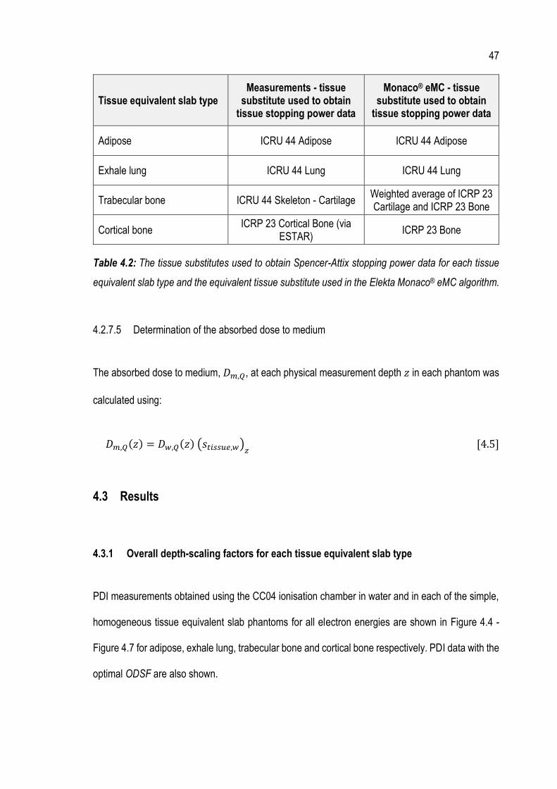
47

Tissue equivalent slab type Measurements - tissue

substitute used to obtain tissue stopping power data

Monaco® eMC - tissue substitute used to obtain

tissue stopping power data

Adipose ICRU 44 Adipose ICRU 44 Adipose

Exhale lung ICRU 44 Lung ICRU 44 Lung

Trabecular bone ICRU 44 Skeleton - Cartilage Weighted average of ICRP 23 Cartilage and ICRP 23 Bone

Cortical bone ICRP 23 Cortical Bone (via

ESTAR) ICRP 23 Bone

Table 4.2: The tissue substitutes used to obtain Spencer-Attix stopping power data for each tissue

equivalent slab type and the equivalent tissue substitute used in the Elekta Monaco® eMC algorithm.

4.2.7.5 Determination of the absorbed dose to medium

The absorbed dose to medium, 𝐷𝑚,𝑄, at each physical measurement depth 𝑧 in each phantom was

calculated using:

𝐷𝑚,𝑄(𝑧) = 𝐷𝑤,𝑄(𝑧) (𝑠𝑡𝑖𝑠𝑠𝑢𝑒,𝑤)𝑧 [4.5]

4.3 Results

4.3.1 Overall depth-scaling factors for each tissue equivalent slab type

PDI measurements obtained using the CC04 ionisation chamber in water and in each of the simple,

homogeneous tissue equivalent slab phantoms for all electron energies are shown in Figure 4.4 -

Figure 4.7 for adipose, exhale lung, trabecular bone and cortical bone respectively. PDI data with the

optimal ODSF are also shown.

48


in the simple, adipose phantom (solid red curve) for all electron energies. Also plotted is the PDI data

as measured in the simple, adipose phantom with the optimal ODSF applied to the physical

measurement depths (dashed red curve).


in the simple, exhale lung phantom (solid red curve) for all electron energies. Also plotted is the PDI

data as measured in the simple, exhale lung phantom with the optimal ODSF applied to the physical


49


in the simple, trabecular bone phantom (solid red curve) for all electron energies. Also plotted is the

PDI data as measured in the simple, trabecular bone phantom with the optimal ODSF applied to the

physical measurement depths (dashed red curve).


in the simple, cortical bone phantom (solid red curve) for all electron energies. Also plotted is the PDI

data as measured in the simple, cortical bone phantom with the optimal ODSF applied to the physical


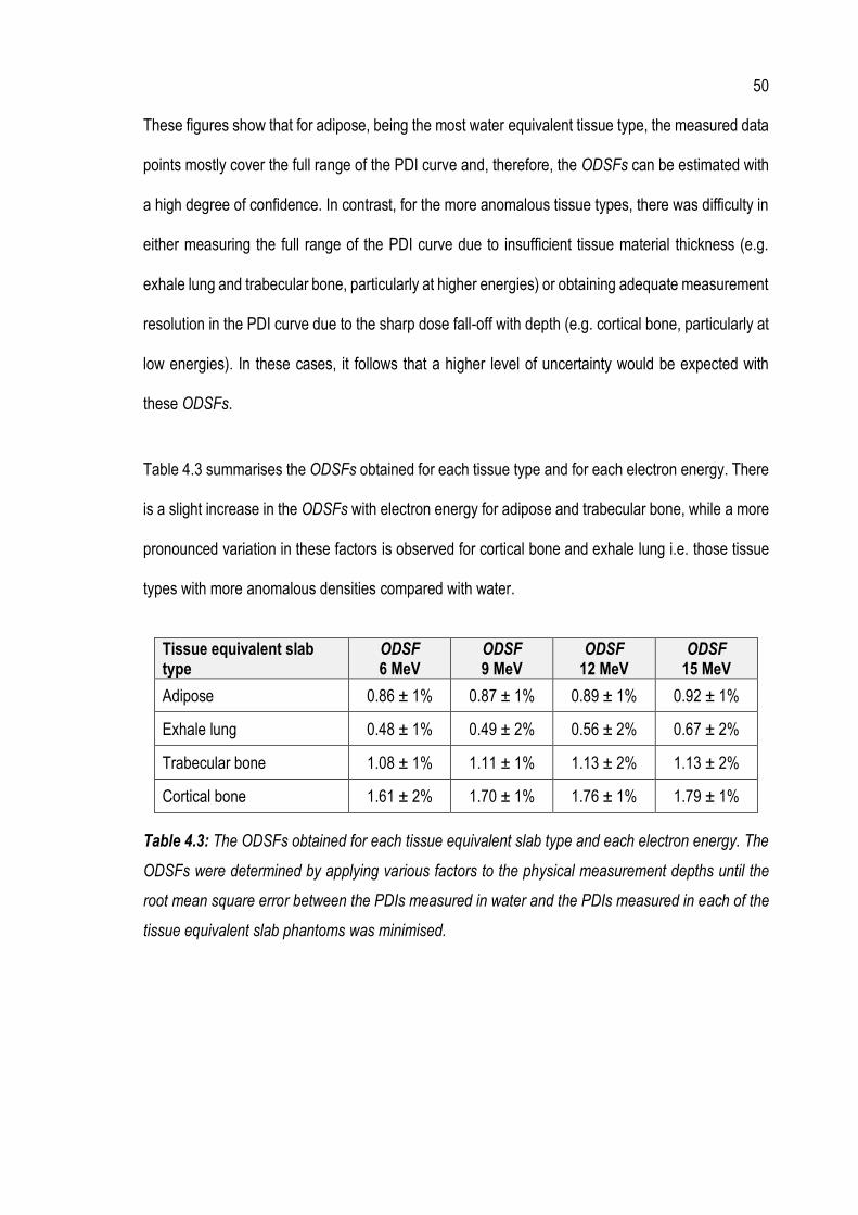
50

These figures show that for adipose, being the most water equivalent tissue type, the measured data

points mostly cover the full range of the PDI curve and, therefore, the ODSFs can be estimated with

a high degree of confidence. In contrast, for the more anomalous tissue types, there was difficulty in

either measuring the full range of the PDI curve due to insufficient tissue material thickness (e.g.

exhale lung and trabecular bone, particularly at higher energies) or obtaining adequate measurement

resolution in the PDI curve due to the sharp dose fall-off with depth (e.g. cortical bone, particularly at

low energies). In these cases, it follows that a higher level of uncertainty would be expected with

these ODSFs.

Table 4.3 summarises the ODSFs obtained for each tissue type and for each electron energy. There

is a slight increase in the ODSFs with electron energy for adipose and trabecular bone, while a more

pronounced variation in these factors is observed for cortical bone and exhale lung i.e. those tissue

types with more anomalous densities compared with water.

Tissue equivalent slab type

ODSF 6 MeV

ODSF 9 MeV

ODSF 12 MeV

ODSF 15 MeV

Adipose 0.86 ± 1% 0.87 ± 1% 0.89 ± 1% 0.92 ± 1%

Exhale lung 0.48 ± 1% 0.49 ± 2% 0.56 ± 2% 0.67 ± 2%

Trabecular bone 1.08 ± 1% 1.11 ± 1% 1.13 ± 2% 1.13 ± 2%

Cortical bone 1.61 ± 2% 1.70 ± 1% 1.76 ± 1% 1.79 ± 1%

Table 4.3: The ODSFs obtained for each tissue equivalent slab type and each electron energy. The

ODSFs were determined by applying various factors to the physical measurement depths until the

root mean square error between the PDIs measured in water and the PDIs measured in each of the

tissue equivalent slab phantoms was minimised.

51

4.3.2 Comparison between Elekta Monaco® eMC dose calculations and measured 𝑫𝒎 in the

simple phantoms

Results comparing the level of agreement between the Elekta Monaco® eMC 𝐷𝑚 dose calculations

and the 𝐷𝑚 as measured in the simple, homogeneous tissue equivalent slab phantoms for all

energies are shown in Figure 4.8 - Figure 4.11 for adipose, exhale lung, trabecular bone and cortical

bone respectively. Table 4.4 quantifies the differences observed for each of the phantoms.

While water equivalent depths were necessary in order to determine stopping power ratios for the

calculation of 𝐷𝑚,𝑄(𝑧), the dose data presented in Figure 4.8 - Figure 4.11 are plotted against the

physical depths in the phantoms.

Figure 4.8: Comparison of the Elekta Monaco® eMC 𝐷𝑚 dose calculation and the 𝐷𝑚 as measured

in the simple, adipose phantom for all electron beam energies.

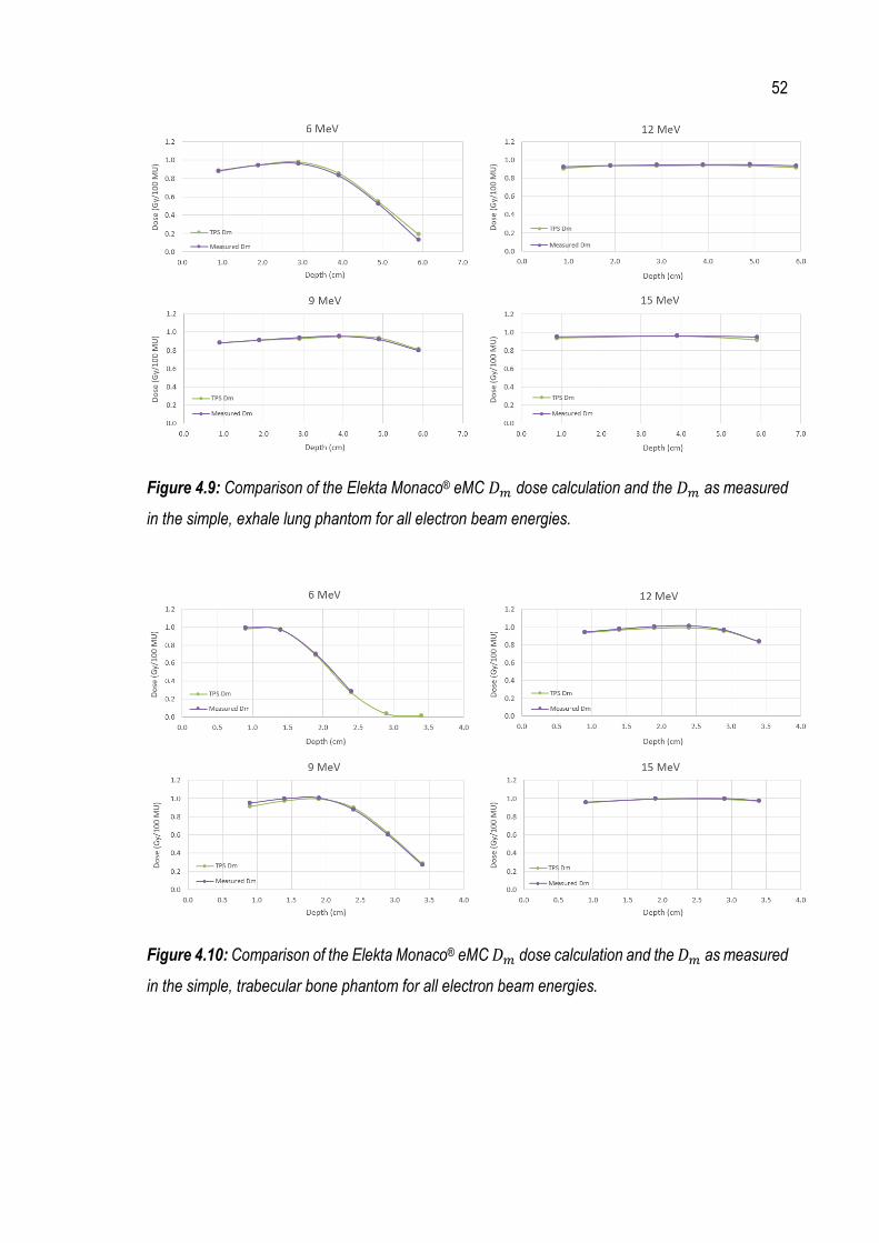
52


in the simple, exhale lung phantom for all electron beam energies.


in the simple, trabecular bone phantom for all electron beam energies.

53


in the simple, cortical bone phantom for all electron beam energies.

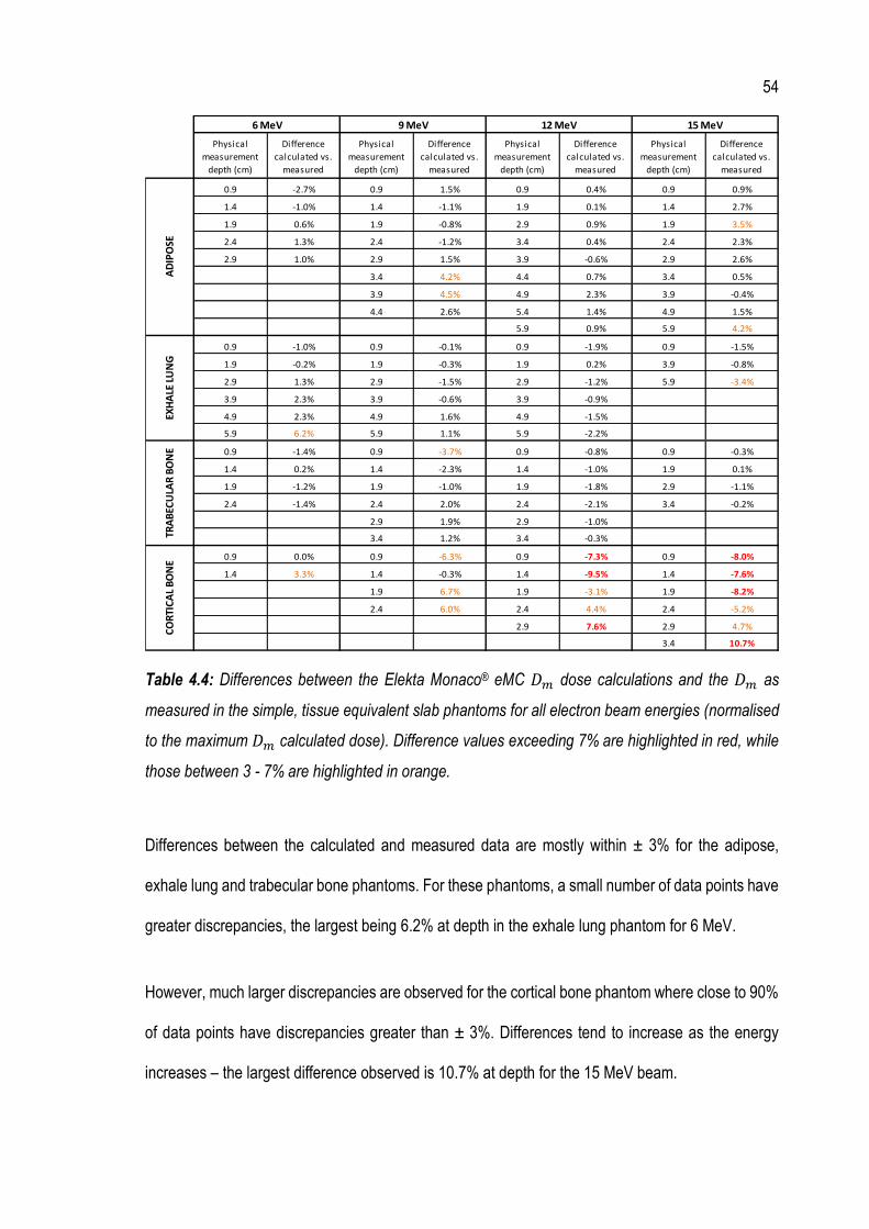
54


measured in the simple, tissue equivalent slab phantoms for all electron beam energies (normalised

to the maximum 𝐷𝑚 calculated dose). Difference values exceeding 7% are highlighted in red, while

those between 3 - 7% are highlighted in orange.

Differences between the calculated and measured data are mostly within ± 3% for the adipose,

exhale lung and trabecular bone phantoms. For these phantoms, a small number of data points have

greater discrepancies, the largest being 6.2% at depth in the exhale lung phantom for 6 MeV.

However, much larger discrepancies are observed for the cortical bone phantom where close to 90%

of data points have discrepancies greater than ± 3%. Differences tend to increase as the energy

increases – the largest difference observed is 10.7% at depth for the 15 MeV beam.

Physical

measurement

depth (cm)

Difference

calculated vs.

measured

Physical

measurement

depth (cm)

Difference

calculated vs.

measured

Physical

measurement

depth (cm)

Difference

calculated vs.

measured

Physical

measurement

depth (cm)

Difference

calculated vs.

measured

0.9 -2.7% 0.9 1.5% 0.9 0.4% 0.9 0.9%

1.4 -1.0% 1.4 -1.1% 1.9 0.1% 1.4 2.7%

1.9 0.6% 1.9 -0.8% 2.9 0.9% 1.9 3.5%

2.4 1.3% 2.4 -1.2% 3.4 0.4% 2.4 2.3%

2.9 1.0% 2.9 1.5% 3.9 -0.6% 2.9 2.6%

3.4 4.2% 4.4 0.7% 3.4 0.5%

3.9 4.5% 4.9 2.3% 3.9 -0.4%

4.4 2.6% 5.4 1.4% 4.9 1.5%

5.9 0.9% 5.9 4.2%

0.9 -1.0% 0.9 -0.1% 0.9 -1.9% 0.9 -1.5%

1.9 -0.2% 1.9 -0.3% 1.9 0.2% 3.9 -0.8%

2.9 1.3% 2.9 -1.5% 2.9 -1.2% 5.9 -3.4%

3.9 2.3% 3.9 -0.6% 3.9 -0.9%

4.9 2.3% 4.9 1.6% 4.9 -1.5%

5.9 6.2% 5.9 1.1% 5.9 -2.2%

0.9 -1.4% 0.9 -3.7% 0.9 -0.8% 0.9 -0.3%

1.4 0.2% 1.4 -2.3% 1.4 -1.0% 1.9 0.1%

1.9 -1.2% 1.9 -1.0% 1.9 -1.8% 2.9 -1.1%

2.4 -1.4% 2.4 2.0% 2.4 -2.1% 3.4 -0.2%

2.9 1.9% 2.9 -1.0%

3.4 1.2% 3.4 -0.3%

0.9 0.0% 0.9 -6.3% 0.9 -7.3% 0.9 -8.0%

1.4 3.3% 1.4 -0.3% 1.4 -9.5% 1.4 -7.6%

1.9 6.7% 1.9 -3.1% 1.9 -8.2%

2.4 6.0% 2.4 4.4% 2.4 -5.2%

2.9 7.6% 2.9 4.7%

3.4 10.7%

15 MeV

AD

IPO

SEEX

HA

LE L

UN

GTR

AB

ECU

LAR

BO

NE

CO

RTI

CA

L B

ON

E

6 MeV 9 MeV 12 MeV

55

4.3.3 Comparison between Elekta Monaco® eMC dose calculations and measured 𝑫𝒎 in the

complex phantom

Results comparing the level of agreement between the Elekta Monaco® eMC 𝐷𝑚 dose calculations

and the 𝐷𝑚 as measured in the complex, inhomogeneous tissue equivalent slab phantom are shown

in Figure 4.12 for both the 12 MeV and 15 MeV beams. For reference, Elekta Monaco® eMC 𝐷𝑤 data

are also shown to demonstrate what would be delivered in the case where 𝐷𝑚 based calculations

were not available. Table 4.5 quantifies the differences observed between the Elekta Monaco® eMC

dose calculations and the measured 𝐷𝑚.

While water equivalent depths were necessary in order to determine stopping power ratios for the

calculation of 𝐷𝑚,𝑄(𝑧), the dose data presented in Figure 4.12 are plotted against the physical

depths in the phantom.

56


in the complex, inhomogeneous tissue equivalent slab phantom for 12 MeV and 15 MeV. For

reference, Elekta Monaco® eMC 𝐷𝑤 data are also shown.


measured in the complex, inhomogeneous tissue equivalent slab phantom for 12 MeV and 15 MeV

(normalised to the maximum 𝐷𝑚 calculated dose). Difference values between 3 - 7% are highlighted

in orange. Also shown are the differences between the Elekta Monaco® eMC dose calculations in

terms of 𝐷𝑚 and 𝐷𝑤 (normalised to the maximum 𝐷𝑚 calculated dose).

Physical

measurement

depth (cm)

Tissue type Difference Dm

calculated vs.

measured

Difference Dm

calculated vs.

Dw calculated

Physical

measurement

depth (cm)

Tissue type Difference Dm

calculated vs.

measured

Difference Dm

calculated vs.

Dw calculated

0.9 Adipose 2.0% 0.9% 0.9 Adipose 1.8% 0.9%

1.9 Adipose 0.3% 0.9% 1.9 Adipose -1.7% 0.9%

4.9 Exhale Lung 3.4% 0.9% 4.9 Exhale Lung 0.3% 1.4%

5.9 Exhale Lung 2.4% 0.5% 5.9 Exhale Lung 0.2% 1.2%

6.9 Exhale Lung 0.9% 0.2% 6.9 Exhale Lung -0.1% 0.9%

15 MeV12 MeV

57

Differences between the Elekta Monaco® eMC 𝐷𝑚 dose calculations and the 𝐷𝑚 data as measured

in the complex phantom are mostly within ± 3%. The largest discrepancy observed is 3.4% in the

case of the 12 MeV beam. This data point was located within exhale lung, closest to the trabecular

bone interface.

Differences between the Elekta Monaco® eMC calculated doses in terms of 𝐷𝑤 and 𝐷𝑚 are all less

than 1.5%.

4.4 Discussion

The agreement between 𝐷𝑚 measured in three of the simple, tissue equivalent slab phantoms

(adipose, exhale lung and trabecular bone) with the Elekta Monaco® eMC 𝐷𝑚 calculated data is

mostly within ± 3% for all energies. For these phantoms, data points exceeding a ± 3% discrepancy

are limited to less than 10% of the total measurement points investigated, while no data points exceed

the 7% tolerance as recommended by the AAPM for electron dose calculation algorithms in

inhomogeneous media (Smilowitz et al. 2015).

There is no specific tolerance recommended for basic TPS validation in non-water equivalent

homogeneous phantoms and, furthermore, no tolerance specified for validation in terms of 𝐷𝑚.

However, the results presented here suggest that, in the majority of cases, the Elekta Monaco® eMC

algorithm is able to accurately predict 𝐷𝑚 in simple phantoms of a single tissue type. Additionally,

these results show that the novel method devised here for 𝐷𝑚 calculation using water equivalent

depths provides a robust dosimetry system in most cases.

A clear exception is observed for the simple, cortical bone phantom, where differences between the

measured 𝐷𝑚 and the Elekta Monaco® eMC calculated data are over ± 7% in many cases, with the

58

largest discrepancies (up to ± 10.7%) observed for higher beam energies. The results for cortical

bone may be attributed to the high density of the material (i.e. 1.91 g/cm3). It is expected that cortical

bone would have very different scattering properties as compared with those of water, resulting in a

much greater lateral spread of the beam as it traverses the medium, significantly affecting the dose.

Therefore, the results obtained for the simple, cortical bone phantom highlight the weakness of the

water equivalent depth method for 𝐷𝑚 determination in cases where materials are significantly

different in density from water.

Additionally, the effective point of measurement of the ionisation chamber is unknown in non-water

equivalent materials. However, in all of the data presented here, the effective point of measurement

has been assumed to be as if the chamber was in water (i.e. 1 mm upstream of the cavity centre). In

less dense materials such as adipose and exhale lung, the effective point of measurement of the

chamber would move toward the centre of the chamber, while for denser materials such as trabecular

and cortical bone, the effective point of measurement of the chamber would be closer to the surface

of the phantom. In the case of high density cortical bone, the shift in the effective point of

measurement could be significant and, therefore, may contribute to the poorer results observed for

the simple, cortical bone phantom. Additionally, the effective point of measurement may be depth

dependant as the mean square scattering angle of electrons increases with depth.

The PDI curves (Figure 4.4 - Figure 4.7) suggest an increased level of uncertainty in the ODSFs in

some cases (e.g. exhale lung and trabecular bone, particularly at higher energies and cortical bone,

particularly at low energies). However, this source of error is unlikely to have a significant bearing on

the measured versus calculated 𝐷𝑚 comparisons. The ODSFs were used to calculate water

equivalent depths, which were in turn used to determine the energy of the beam at these depths so

that stopping power data for each tissue type could be obtained. While stopping power data did vary

with energy, the tissue-to-water stopping power ratios, 𝑠𝑡𝑖𝑠𝑠𝑢𝑒,𝑤, did not vary significantly with

59

energy. Therefore, any uncertainty in the estimated most probable energy and ODSFs is unlikely to

translate into significant errors in the tissue-to-water stopping power ratios. For example, given a 2%

uncertainty in the ODSF, the error in tissue-to-water stopping power ratios is estimated to be less

than 0.3%. Furthermore, the use of monoenergetic stopping power data (rather than more accurate

stopping power data based on a polyenergetic spectrum) is unlikely to have a significant impact on

the measured versus calculated 𝐷𝑚 comparisons.

In the case of the complex, inhomogeneous phantom, excellent agreement was observed between

the measured 𝐷𝑚 and the Elekta Monaco® eMC 𝐷𝑚 calculated data. All data points investigated for

both energies were well within the 7% tolerance as recommended by the AAPM for electron dose

calculation algorithms in inhomogeneous media (Smilowitz et al. 2015). These results show that the

Elekta Monaco® eMC algorithm is able to accurately predict 𝐷𝑚 in the clinically realistic scenario

considered. Furthermore, these results add further weight to the accuracy of the water equivalent

depth method developed in this research project to calculate 𝐷𝑚 from measurements of ionisation

in tissue types that are not significantly different in density from water.

The results obtained for the complex, inhomogeneous phantom also show only small differences

(less than 1.5%) between the Elekta Monaco® eMC doses calculated in terms of 𝐷𝑚 and 𝐷𝑤.

Significant differences would only be expected for cases involving materials with a chemical

composition substantially different from that of water (e.g. cortical bone). Therefore, in most clinical

scenarios (i.e. those involving near water equivalent media), the differences between dose calculated

in terms of 𝐷𝑚 and 𝐷𝑤 are insignificant. However, clinical practice shows that significant differences

in the number of MU to be delivered to patients based on a 𝐷𝑤 measured output factor and that

calculated in terms of 𝐷𝑚 do in fact occur. (This aspect of the research project is discussed in more

detail in Section 5.3.1). It is likely that these differences are primarily due to the increase in accuracy

of the dose calculation used, rather than fundamental differences between 𝐷𝑤 and 𝐷𝑚. The increase

60

in accuracy results from the use of the patient CT dataset to obtain the patient contour and density

information, as opposed to the use of a measured output factor based on a flat, homogeneous plastic

water slab phantom.

4.5 Conclusions

The results show that the 𝐷𝑚 calculation in the Elekta Monaco® eMC algorithm is able to accurately

predict the dose in most cases (both simple and complex) involving non-water equivalent media. In

the case of simple, homogeneous phantoms involving a single tissue type of adipose, exhale lung or

trabecular bone, the level of agreement between the measured 𝐷𝑚 and the Elekta Monaco® eMC

𝐷𝑚 calculated data is mostly within ± 3%. In the more clinically realistic case involving three tissue

types, agreement was found to be within ± 3.4%. However, large discrepancies of up to ± 10.7%

were observed for the simple, cortical bone phantom.

The novel method devised here for 𝐷𝑚 determination using water equivalent depths provides a

robust dosimetry system in cases where tissue types are not significantly different in density from

water (i.e. > 0.5 g/cm3 and < 1.5 g/cm3). However, the poor cortical bone results highlight the

weakness of the water equivalent depth method in high density tissues. This is likely due to the

different scattering properties of cortical bone as compared with those of water and the unknown

effective point of measurement of the ionisation chamber when in non-water equivalent materials.

While it has not been experimentally verified, it can be expected that similar behaviour would be

observed for very low density materials such as inhale lung (density 0.2 g/cm3).

The 𝐷𝑚 validation results presented here suggest that the Elekta Monaco® eMC 𝐷𝑚 calculation is

accurate in most of the clinical scenarios considered. However, in order to fully validate the algorithm,

another method is required for very high density and very low density materials. The most accurate

61

validation method would involve full Monte Carlo modelling to correctly account for the unique

scattering properties of the materials and to determine the energy spectrum and polyenergetic tissue-

to-water stopping power ratios at each measurement depth. However, this work is beyond the scope

of the project.

In most cases, the difference in the number of MU to be delivered in patient treatments based on

measured output factors in water compared with those calculated in terms of 𝐷𝑚 is likely due to the

increase in accuracy of the dose calculation (e.g. more realistic patient geometry), rather than

fundamental differences between 𝐷𝑤 and 𝐷𝑚.

62

5 Statistical analysis of patient acute toxicity data

This chapter addresses research question 2 by examining the effect on patient outcomes from using

the Elekta Monaco® eMC 𝐷𝑚-based MU in clinical treatments.

5.1 Introduction

A statistical analysis of patient data was undertaken to assess the effect of the change in clinical

practice from using measured 𝐷𝑤-based MU (i.e. MU measured in a flat, homogenous plastic water

phantom) to calculated 𝐷𝑚-based MU in electron treatments in terms of patient acute skin toxicity.

Patient acute toxicity and treatment-related data from the electronic medical record (eMR) have been

collected and summarised for two purposes.

• Undertaking a cohort study to determine whether there is a statistically significant difference

in acute skin toxicity for patients treated with the measured 𝐷𝑤-based MU compared with a

similar cohort of patients treated with the Elekta Monaco® eMC 𝐷𝑚-based MU. This

determination will be achieved using the Cochran-Armitage test for linear trend.

• Assessing the relationship between acute toxicity grade and various clinical factors to

identify predictors of radiation-induced acute skin toxicity. This assessment will be achieved

through the development of binary logistic regression models.

63


5.2.1 Patient data collection and summary statistics

The eMR used at MNCCI is Elekta’s MOSAIQ®. A full list of patients treated with electrons at MNCCI

from 2016 (when the Elekta Monaco® eMC algorithm was commissioned for clinical use) up until

2019 was extracted from MOSAIQ®. Patients recruited into the cohort study needed to meet the

following eligibility criteria.

• Have been treated with electrons, using any of the available electron beams: 6 MeV, 9 MeV,

12 MeV, 15 MeV or 18 MeV.

• Have been treated for skin cancer: Squamous cell carcinoma (SCC), Basal cell carcinoma

(BCC), Melanoma or skin cancer - other.

• Have no concurrent photon treatment.

• Have maximum baseline toxicity grades of less than 2.

• Have at least one acute toxicity assessment recorded during their treatment or within

90 days of their treatment finish date.

• Have been treated at any one of the three MNCCI cancer centres: Port Macquarie,

Coffs Harbour or Lismore.

Patients treated with electron breast boosts have not been included in the cohort study as these

patients also undergo treatment with photon fields. To reduce the risk of confounding factors caused

by the photon fields, the decision was made to limit the cohort study to only skin cancer patients


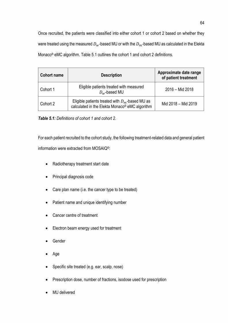
64

Once recruited, the patients were classified into either cohort 1 or cohort 2 based on whether they

were treated using the measured 𝐷𝑤-based MU or with the 𝐷𝑚-based MU as calculated in the Elekta

Monaco® eMC algorithm. Table 5.1 outlines the cohort 1 and cohort 2 definitions.

Cohort name Description Approximate date range

of patient treatment

Cohort 1 Eligible patients treated with measured

𝐷𝑤-based MU 2016 – Mid 2018

Cohort 2 Eligible patients treated with 𝐷𝑚-based MU as

calculated in the Elekta Monaco® eMC algorithm Mid 2018 – Mid 2019

Table 5.1: Definitions of cohort 1 and cohort 2.

For each patient recruited to the cohort study, the following treatment-related data and general patient

information were extracted from MOSAIQ®:

• Radiotherapy treatment start date

• Principal diagnosis code

• Care plan name (i.e. the cancer type to be treated)

• Patient name and unique identifying number

• Cancer centre of treatment

• Electron beam energy used for treatment

• Gender

• Age

• Specific site treated (e.g. ear, scalp, nose)

• Prescription dose, number of fractions, isodose used for prescription

• MU delivered

65

• MU calculation method: measured 𝐷𝑤-based or calculated 𝐷𝑚-based

To record information on patient acute toxicity, MNCCI uses the Common Terminology Criteria for

Adverse Events (CTCAE) Version 4 (U.S Department of Health and Human Services 2009). In this

guideline, adverse events are defined as:

“Any unfavorable and unintended sign (including an abnormal laboratory finding), symptom, or

disease temporarily associated with the use of a medical treatment or procedure that may or may not

be considered related to the medical treatment or procedure. An adverse event is a term that is a

unique representation of a specific event used for medical documentation and scientific analyses.”

In the context of this study, adverse events can be thought of as different categories of skin acute

toxicity signs and symptoms that result from the patient’s electron treatment. The adverse events

assessed in this study were rash, infection, pain, telangiectasia, soft tissue fibrosis, alopecia and skin

ulceration. Each of these adverse events is described in Table 5.2.

According to the CTCAE guidelines, each adverse event is graded for severity between 1 and 5.

Table 5.3 provides general descriptions of each grade.

66

Adverse event (skin-related acute toxicities)

Description

Rash A disorder characterised by the presence of macules (flat) and papules (elevated).

Infection A disorder characterised by an infectious process involving the skin.

Pain A disorder characterised by a marked discomfort sensation in the skin.

Telangiectasia A disorder characterised by local dilatation of small vessels resulting in red discoloration of the skin or mucous membranes.

Soft tissue fibrosis A disorder characterised by fibrotic degeneration of the superficial soft tissues.

Alopecia A disorder characterised by a decrease in density of hair compared to normal for a given individual at a given age and body location.

Skin ulceration A disorder characterised by circumscribed, inflammatory and necrotic erosive lesion on the skin.

Table 5.2: Definitions of skin-related adverse events, taken from CTCAE Version 4 (U.S Department

of Health and Human Services 2009).

Grade of adverse event

Description of grade

Grade 1 Mild; asymptomatic or mild symptoms; clinical or diagnostic observations only; intervention not indicated.

Grade 2 Moderate; minimal, local or noninvasive intervention indicated; limiting age-appropriate instrumental Activities of Daily Living (ADL). *

Grade 3 Severe or medically significant but not immediately life-threatening; hospitalisation or prolongation of hospitalisation indicated; disabling; limiting self-care ADL. **

Grade 4 Life threatening consequences; urgent intervention indicated.

Grade 5 Death related to the adverse event.

Table 5.3: General definitions of severity grades, taken from CTCAE Version 4 (U.S Department of

Health and Human Services 2009), where *Instrumental ADL refer to preparing meals, shopping for

groceries or clothes, using the telephone, managing money, etc. and **Self-care ADL refer to bathing,

dressing and undressing, feeding self, using the toilet, taking medications, and not bedridden.

67

At MNCCI, a baseline toxicity assessment is carried out before the patient’s radiotherapy treatment

start date, whereby each of the adverse events in Table 5.2 is given a severity score using the

definitions in Table 5.3. The baseline toxicity assessment assesses and records any skin toxicities

the patient may have that are not caused by the radiation treatment (but may or may not be related

to the cancer being treated). Acute toxicity assessments then occur at regular intervals during the

patient’s treatment, and up to 90 days after their treatment is completed. The overall frequency of

acute toxicity assessments is approximately every 2 - 3 weeks.

For the purposes of patient data collection and analysis, the maximum scores for both baseline and

acute toxicity assessments were recorded for each adverse event. For example, a patient may have

had 10 acute toxicity assessments recorded during and after their treatment, with rash grades varying

between 1 and 3. In this example, the grade that would be recorded for the acute toxicity assessment

rash adverse event would be 3.

All patient data was collated and stored in a Microsoft Excel spreadsheet. Summary statistics, relating

to general patient information and treatment characteristics were performed in Microsoft Excel to gain

an overall impression of the dataset.

5.2.2 Cochran-Armitage test for linear trend

In order to determine whether there is a statistically significant difference in acute toxicity for patients

treated with the measured 𝐷𝑤-based MU as compared with patients treated with the Elekta Monaco®

eMC 𝐷𝑚-based MU, the Cochran-Armitage test for linear trend (Armitage 1955; Cochran 1954) was

calculated using Genstat software.

68

This statistical test is a modified form of a chi-squared test and is often used in epidemiology and

dose-response studies to test for trends among binomial proportions. Its purpose is to investigate the

presence of an association between a variable with two categories (i.e. a binary variable) and an

explanatory variable with n categories. In the context of this cohort study, the binary variable is cohort

(i.e. either cohort 1 or cohort 2) while the explanatory variable is the acute toxicity grade. The acute

toxicity grade takes into account the baseline toxicity score: a subtraction was performed between

the maximum acute toxicity grade and the maximum baseline grade, herein referred to as the

“difference grade”.

The test was performed for each adverse event individually, and for all adverse events combined.

The input data for the test were provided as “2 x n” tables of percentage frequency count for each

adverse event, and for all adverse events combined i.e. in each case, the percentage of patients

experiencing each of the various difference grades, n, are tabulated for both cohort 1 and cohort 2.

These data tables were entered directly into the Genstat software for processing.

The null hypothesis, H0, for the Cochran-Armitage test for linear trend is the hypothesis of no trend,

which means that the binomial proportion is the same for all levels of the explanatory variable. The

alternative hypothesis, H1, is that there is a linear trend in binomial proportions across increasing

levels of the explanatory variable. The results of the test are presented as p-values: p-values under

0.05, corresponding to a 95% confidence interval (CI), are considered statistically significant (i.e.

where the null hypothesis can be rejected). For p-values larger than 0.05, the null hypothesis cannot

be rejected and, therefore, statistical significance cannot be concluded.

69

5.2.3 Binary logistic regression models

A binary logistic regression model for each adverse event was created in IBM® SPSS software to

assess the effect of various predictors on acute toxicity grade. Binary logistic regression works by

assessing the relationship between a dependent binary variable (i.e. the “outcome”) and one or more

independent variables called predictors (i.e. explanatory variables that are suspected of influencing

the outcome of the dependent variable). The goal of logistic regression is to find the best fitting model

to describe the relationship between the dependent binary variable of interest and the set of

independent predictor/explanatory variables.

Figure 5.1 shows the concept of binary logistic regression. For this analysis, the dependent binary

variable is acute toxicity for the specific adverse event (i.e. present or not present), while the

predictors include cohort (i.e. cohort 1 or cohort 2), baseline toxicity for the specific adverse event

(i.e. either present or not present) and “tissue category”.

Tissue category has three possible classifications: soft tissue, bone or air. It essentially describes if

the patient's treatment site consists mostly of soft tissue or has bone or air inhomogeneities present.

For example, a scalp treatment would be categorised as bone, an ear/nose treatment would be

categorised as air while an abdomen treatment would be considered soft tissue. The rationale for this

predictor was that such tissue inhomogeneities may lead to larger MU discrepancies between 𝐷𝑤

and 𝐷𝑚 and hence greater differences in acute toxicity.

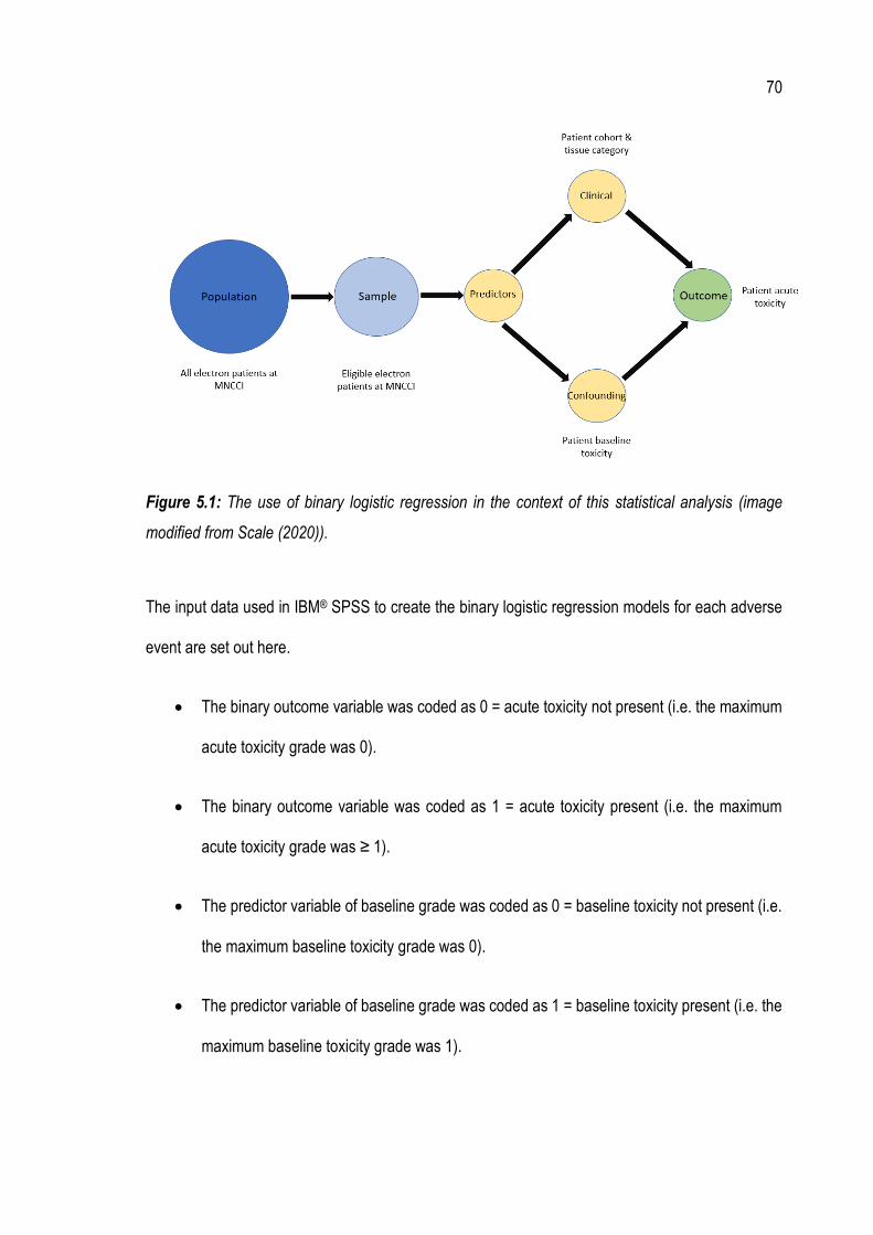
70

Figure 5.1: The use of binary logistic regression in the context of this statistical analysis (image

modified from Scale (2020)).

The input data used in IBM® SPSS to create the binary logistic regression models for each adverse

event are set out here.

• The binary outcome variable was coded as 0 = acute toxicity not present (i.e. the maximum

acute toxicity grade was 0).

• The binary outcome variable was coded as 1 = acute toxicity present (i.e. the maximum

acute toxicity grade was ≥ 1).

• The predictor variable of baseline grade was coded as 0 = baseline toxicity not present (i.e.

the maximum baseline toxicity grade was 0).

• The predictor variable of baseline grade was coded as 1 = baseline toxicity present (i.e. the

maximum baseline toxicity grade was 1).

71

• The predictor variable of cohort was coded as 0 for cohort 1 and coded as 1 for cohort 2 (i.e.

cohort 1 acts as the reference category).

• The polychotomous predictor variable of tissue category was coded as 0 = soft tissue, 1 =

bone, 2 = air, with soft tissue acting as the reference category.

The model output data are given in the form of an adjusted odds ratio, Exp B, with lower and upper

limits of the 95% CI associated with the adjusted odds ratio, for each of the predictor variables. A

p-value is also reported. The model output results for each predictor variable are interpreted in the

following way (Scale 2020).

• If the 95% CI associated with the adjusted odds ratio crosses over 1.0, then there is a non-

significant association. The p-value associated with these variables will also be greater than

0.05.

• If the adjusted odds ratio is above 1.0 and the 95% CI is entirely above 1.0, then exposure

to the predictor increases the odds of the outcome.

• If the adjusted odds ratio is below 1.0 and the 95% CI is entirely below 1.0, then exposure

to the predictor decreases the odds of the outcome.

The binary logistic regression model for each adverse event also produces scatter plots of the raw

residuals, which show the differences between the observed and predicted probabilities of the model,

plotted against the predicted probability. These scatter plots help to subjectively assess the

assumption of linearity in the model (and hence the validity of the model), based on the symmetry of

points above and below a straight line as well as the distribution of points.

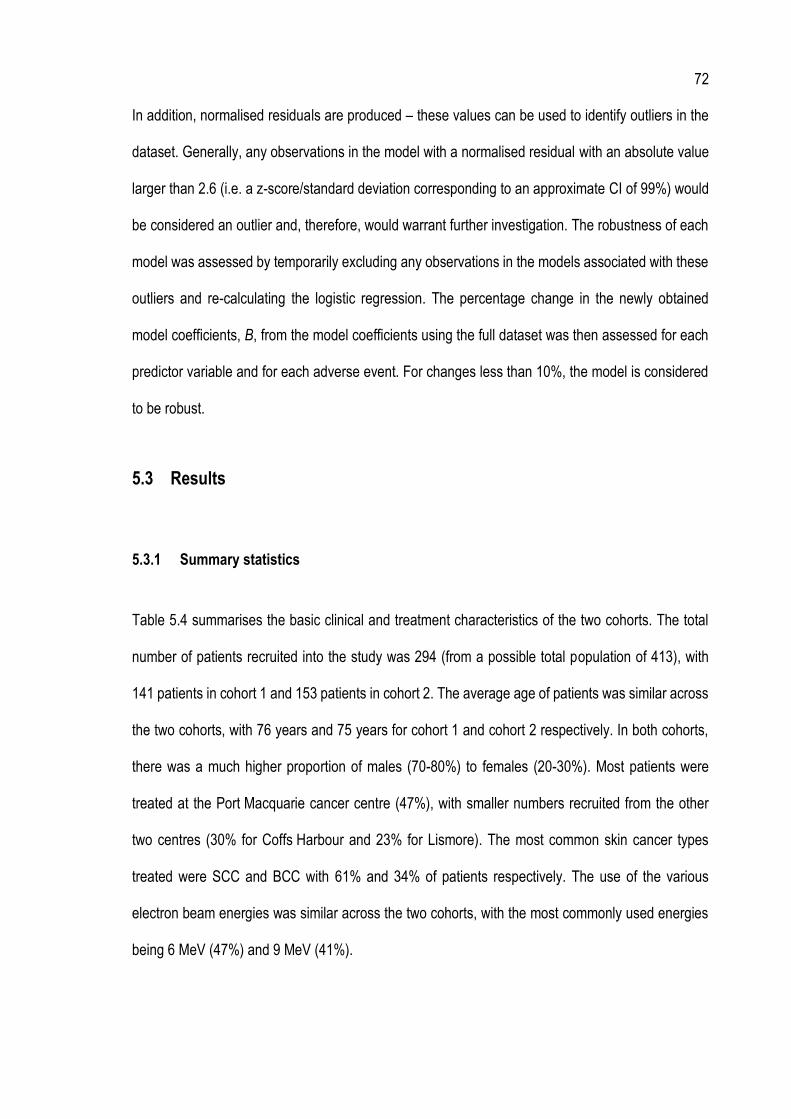
72

In addition, normalised residuals are produced – these values can be used to identify outliers in the

dataset. Generally, any observations in the model with a normalised residual with an absolute value

larger than 2.6 (i.e. a z-score/standard deviation corresponding to an approximate CI of 99%) would

be considered an outlier and, therefore, would warrant further investigation. The robustness of each

model was assessed by temporarily excluding any observations in the models associated with these

outliers and re-calculating the logistic regression. The percentage change in the newly obtained

model coefficients, B, from the model coefficients using the full dataset was then assessed for each

predictor variable and for each adverse event. For changes less than 10%, the model is considered

to be robust.

5.3 Results

5.3.1 Summary statistics

Table 5.4 summarises the basic clinical and treatment characteristics of the two cohorts. The total

number of patients recruited into the study was 294 (from a possible total population of 413), with

141 patients in cohort 1 and 153 patients in cohort 2. The average age of patients was similar across

the two cohorts, with 76 years and 75 years for cohort 1 and cohort 2 respectively. In both cohorts,

there was a much higher proportion of males (70-80%) to females (20-30%). Most patients were

treated at the Port Macquarie cancer centre (47%), with smaller numbers recruited from the other

two centres (30% for Coffs Harbour and 23% for Lismore). The most common skin cancer types

treated were SCC and BCC with 61% and 34% of patients respectively. The use of the various

electron beam energies was similar across the two cohorts, with the most commonly used energies

being 6 MeV (47%) and 9 MeV (41%).

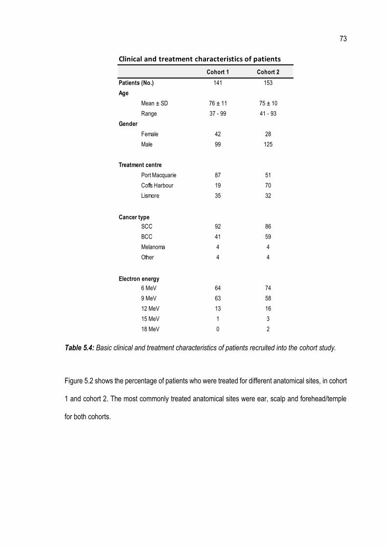
73

Table 5.4: Basic clinical and treatment characteristics of patients recruited into the cohort study.

Figure 5.2 shows the percentage of patients who were treated for different anatomical sites, in cohort

1 and cohort 2. The most commonly treated anatomical sites were ear, scalp and forehead/temple

for both cohorts.

Clinical and treatment characteristics of patients

Cohort 1 Cohort 2

Patients (No.) 141 153

Age

Mean ± SD 76 ± 11 75 ± 10

Range 37 - 99 41 - 93

Gender

Female 42 28

Male 99 125

Treatment centre

Port Macquarie 87 51

Coffs Harbour 19 70

Lismore 35 32

Cancer type

SCC 92 86

BCC 41 59

Melanoma 4 4

Other 4 4

Electron energy

6 MeV 64 74

9 MeV 63 58

12 MeV 13 16

15 MeV 1 3

18 MeV 0 2

74

Figure 5.2: The percentage of patients treated for different anatomical sites in cohort 1 and cohort

2.

While patients in cohort 1 were treated with the measured 𝐷𝑤-based MU, 𝐷𝑚-based dose

calculations in the Elekta Monaco® eMC algorithm were also carried out for these patients, thereby

providing a direct comparison between the measured 𝐷𝑤-based MU and the calculated 𝐷𝑚-based

MU. This data is summarised in Figure 5.3. On average, the difference between the measured

𝐷𝑤-based MU and the calculated 𝐷𝑚-based MU was 2.5% (with the 𝐷𝑚-based MU as calculated in

the Elekta Monaco® eMC algorithm being higher). However, in certain cases, differences of up to

20% were observed. Generally, these large differences were for cases involving high density cortical

bone (such as in scalp treatments) or for cases involving air inhomogeneities (such as in nose and

ear treatments).

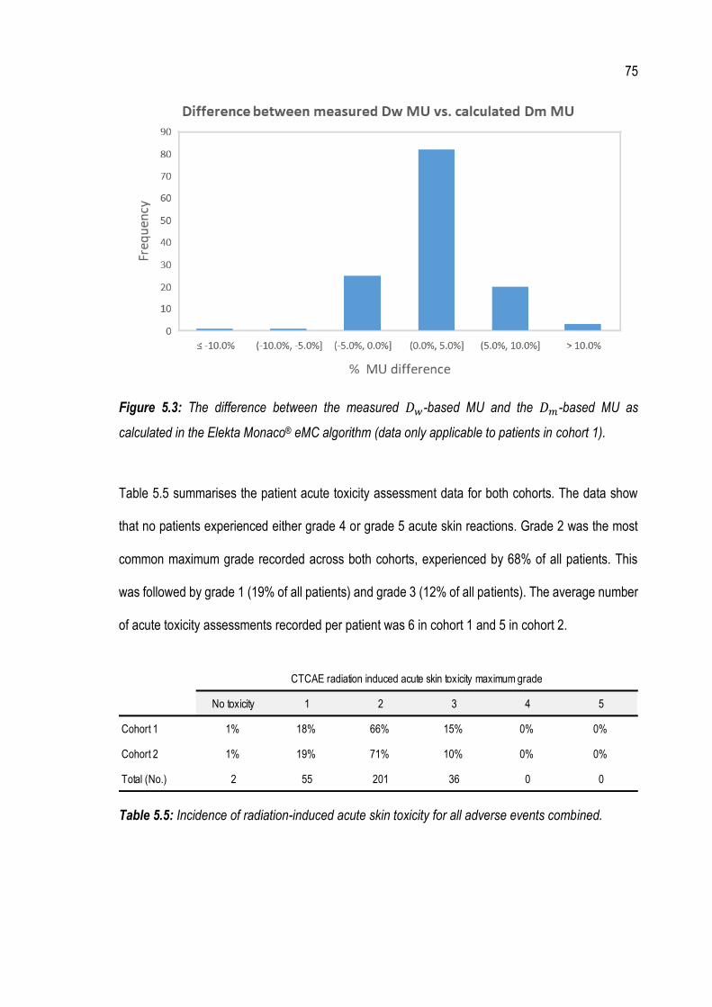
75

Figure 5.3: The difference between the measured 𝐷𝑤-based MU and the 𝐷𝑚-based MU as

calculated in the Elekta Monaco® eMC algorithm (data only applicable to patients in cohort 1).

Table 5.5 summarises the patient acute toxicity assessment data for both cohorts. The data show

that no patients experienced either grade 4 or grade 5 acute skin reactions. Grade 2 was the most

common maximum grade recorded across both cohorts, experienced by 68% of all patients. This

was followed by grade 1 (19% of all patients) and grade 3 (12% of all patients). The average number

of acute toxicity assessments recorded per patient was 6 in cohort 1 and 5 in cohort 2.

Table 5.5: Incidence of radiation-induced acute skin toxicity for all adverse events combined.

No toxicity 1 2 3 4 5

Cohort 1 1% 18% 66% 15% 0% 0%

Cohort 2 1% 19% 71% 10% 0% 0%

Total (No.) 2 55 201 36 0 0

CTCAE radiation induced acute skin toxicity maximum grade

76

A more detailed summary of the patient acute toxicity assessment data, broken down into each

adverse event, is presented in Table 5.6, and shown graphically in Figure 5.4 - Figure 5.10. The most

commonly experienced adverse events included rash and pain.

77

Table 5.6: The percentage of patients experiencing either no toxicity or maximum acute toxicity grades of 1 to 5, in each cohort and for each adverse event.

Adverse Event Cohort 1 Cohort 2 Cohort 1 Cohort 2 Cohort 1 Cohort 2 Cohort 1 Cohort 2 Cohort 1 Cohort 2 Cohort 1 Cohort 2

Rash 1% 1% 21% 22% 64% 67% 14% 10% 0% 0% 0% 0%

Infection 82% 88% 15% 7% 4% 5% 0% 0% 0% 0% 0% 0%

Pain 34% 50% 60% 44% 6% 6% 0% 0% 0% 0% 0% 0%

Telangiectasia 94% 93% 6% 7% 0% 0% 0% 0% 0% 0% 0% 0%

Soft tissue fibrosis 67% 77% 32% 21% 1% 2% 0% 0% 0% 0% 0% 0%

Alopecia 67% 69% 31% 31% 1% 1% 0% 0% 0% 0% 0% 0%

Skin ulceration 87% 89% 6% 4% 7% 7% 1% 1% 0% 0% 0% 0%

Grade 5No toxicity Grade 1 Grade 2 Grade 3 Grade 4

78


acute skin toxicity grades of 1 to 5 for the rash adverse event.


acute skin toxicity grades of 1 to 5 for the infection adverse event.

79


acute skin toxicity grades of 1 to 5 for the pain adverse event.


acute skin toxicity grades of 1 to 5 for the telangiectasia adverse event.

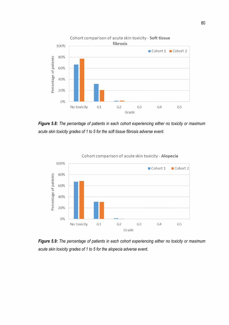
80


acute skin toxicity grades of 1 to 5 for the soft tissue fibrosis adverse event.


acute skin toxicity grades of 1 to 5 for the alopecia adverse event.

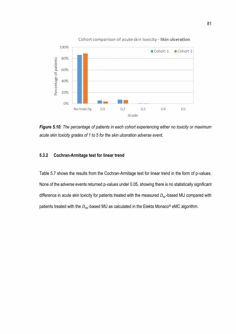
81


acute skin toxicity grades of 1 to 5 for the skin ulceration adverse event.

5.3.2 Cochran-Armitage test for linear trend

Table 5.7 shows the results from the Cochran-Armitage test for linear trend in the form of p-values.

None of the adverse events returned p-values under 0.05, showing there is no statistically significant

difference in acute skin toxicity for patients treated with the measured 𝐷𝑤-based MU compared with

patients treated with the 𝐷𝑚-based MU as calculated in the Elekta Monaco® eMC algorithm.

82

Adverse event p-value

Rash 0.736

Infection 0.472

Pain 0.383

Telangiectasia 0.799

Soft tissue fibrosis 0.765

Alopecia 0.994

Skin ulceration 0.869

ALL EVENTS 0.646

Table 5.7: p-values from the Cochran-Armitage test for linear trend, as calculated in Genstat, for

each individual adverse event and for all events combined.

5.3.3 Binary logistic regression models

Table 5.8 summarises the results of the binary logistic regression analysis for each adverse event.

By interpreting the adjusted odds ratios and associated upper and lower limits of the 95% CIs, the

following significant results were obtained from the models.

• Baseline toxicity predictor variable: for multiple adverse events (infection, pain,

telangiectasia, soft tissue fibrosis and alopecia), there is a significant correlation between

baseline toxicity grade and acute toxicity grade. The models show that having a higher

baseline toxicity grade increases the chances of having increased levels of acute toxicity.

• Cohort predictor variable: for the pain adverse event, there is a significant correlation

between cohort and acute toxicity grade. The model shows that patients in cohort 2

experienced lower levels of pain than those patients in cohort 1.

83

• Tissue category predictor variable: for the pain and alopecia adverse events, there is a

significant correlation between bone-related treatment sites and acute toxicity grade. In

terms of the pain adverse event, the model showed that patients with a bone treatment site

were likely to experience lower levels of acute toxicity, while for the alopecia adverse event,

patients were likely to experience increased acute toxicity.

Figure 5.11 - Figure 5.17 show scatter plots of the raw residuals against the predicted probability for

each adverse event. In all cases, linearity can be assumed given the points are mostly symmetric

above and below a straight line and the points are mostly evenly distributed along a line.

Table 5.9 summarises the number of outliers (i.e. normalised residuals with an absolute value larger

than 2.6) in each of the models. All models had at least 1 outlier, with significant numbers observed

for the telangiectasia and skin ulceration adverse events (15 and 26 outliers respectively). As

described in Section 5.2.3, the binary logistic regression models were calculated with the outliers

excluded, so that the model coefficients could be compared with the full dataset and, therefore, the

degree of robustness of each model could be assessed. The final results from this test are

summarised in the “Model Robust?” column of Table 5.8. Of the eight significant results obtained,

three can be considered to be associated with a robust model. These are pain (cohort predictor

variable), soft tissue fibrosis (baseline predictor variable) and alopecia (bone tissue category

predictor variable).

For the rash adverse event, the degree of model robustness could not be computed. This adverse

event had two outliers: one from cohort 1 and one from cohort 2. These were the only model

observations with the acute toxicity outcome variable of zero, meaning that after removal of these

outliers, there were no model observations left with an acute toxicity outcome variable of zero.

84

Therefore, the regression analysis could not be calculated as it requires exactly two values for the

dependent outcome variable.

85

Table 5.8: A summary of results from the binary logistic regression models for each adverse event. Significant results are highlighted in green.

Lower Upper

Rash

Cohort 3.40 0.19 62.08 No N/A

Baseline 1134403.92 0.00 No N/A

Tissue Category - Bone 22285346.96 0.00 No N/A

Tissue Category - Air 2.61 0.14 47.57 No N/A

Infection

Cohort 0.70 0.33 1.51 No Not Robust

Baseline 8.70 3.18 23.83 Yes Not Robust Having a higher baseline score increases the chance of having greater acute toxicity

Tissue Category - Bone 0.80 0.30 2.12 No Not Robust

Tissue Category - Air 1.05 0.40 2.72 No Robust

Pain

Cohort 0.58 0.35 0.98 Yes Robust Patients in cohort 2 have a decreased chance of having greater acute toxicity


Tissue Category - Bone 0.39 0.19 0.82 Yes Not Robust Patients with a bone treatment site have a decreased chance of having greater acute toxicity

Tissue Category - Air 0.69 0.32 1.47 No Not Robust

Telangiectasia





Soft tissue fibrosis


Baseline 3.32 1.77 6.21 Yes Robust Having a higher baseline score increases the chance of having greater acute toxicity



Alopecia



Tissue Category - Bone 4.90 1.95 12.36 Yes Robust Patients with a bone treatment site have a increased chance of having greater acute toxicity


Skin ulceration


Baseline 2.50 0.58 10.70 No Not Robust



Yes

Yes

Yes

Interpretation (for significant results)Model Robust?Assumpition of

Linearity?

Yes

Yes

Yes

Yes

95% C.I for Exp (B)Adverse Event Predictor Exp (B) Significant Result?

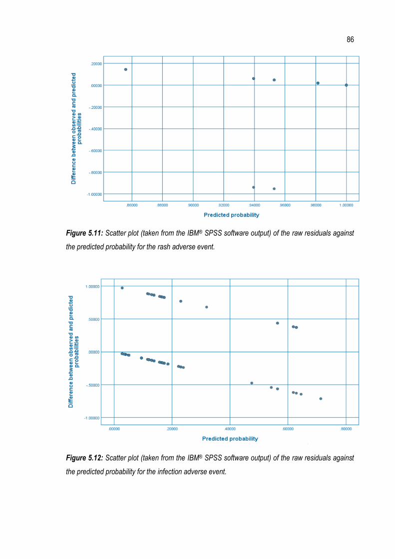
86


the predicted probability for the rash adverse event.


the predicted probability for the infection adverse event.

87


the predicted probability for the pain adverse event.


the predicted probability for the telangiectasia adverse event.

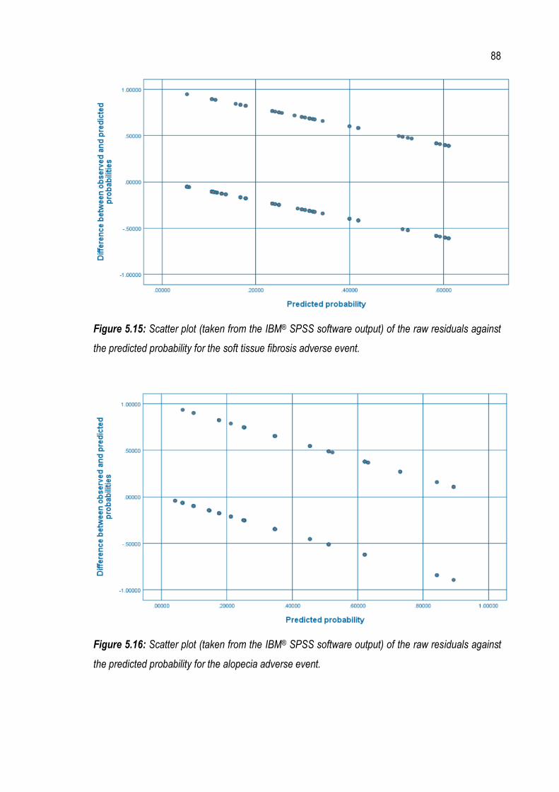
88


the predicted probability for the soft tissue fibrosis adverse event.


the predicted probability for the alopecia adverse event.

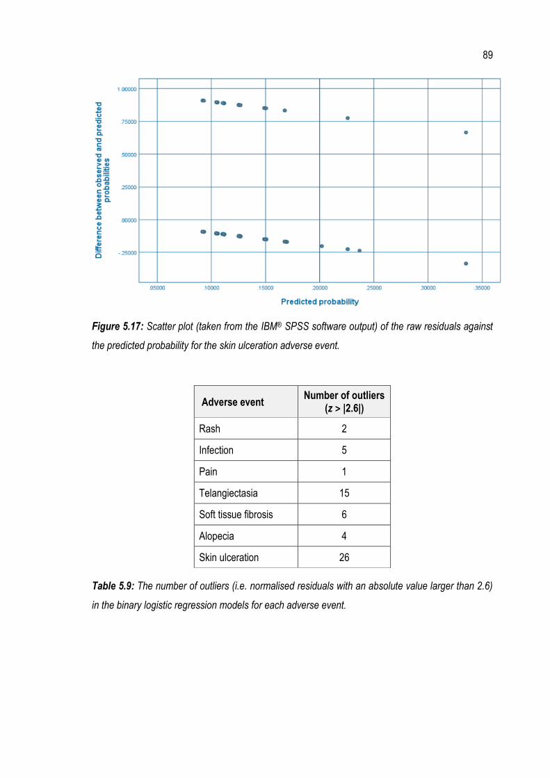
89


the predicted probability for the skin ulceration adverse event.

Adverse event Number of outliers

(z > |2.6|)

Rash 2

Infection 5

Pain 1

Telangiectasia 15

Soft tissue fibrosis 6

Alopecia 4

Skin ulceration 26

Table 5.9: The number of outliers (i.e. normalised residuals with an absolute value larger than 2.6)

in the binary logistic regression models for each adverse event.

90

5.4 Discussion

General patient and treatment characteristics such as age, gender, cancer type, treatment site and

electron energy were similar in both cohorts, suggesting that the potential for these characteristics to

act as confounding factors in this statistical analysis is low. The exception is the cancer centre in

which the patients were treated. A larger percentage of patients was treated at Port Macquarie (47%)

compared with those treated at the other two centres. While the three cancer centres act across a

common health network in terms of procedures, cross-site involvement and data sharing, there is still

the possibility of centre-specific differences in the way that patient acute toxicity data is assessed

and recorded. Therefore, the potential exists for a small bias in the data. However, this potential bias

is offset to a large degree by having patients recruited into the study across three different cancer

centres over a broad geographical area, allowing for a larger and more representative sample of the

overall population.

In terms of interpreting and recording patient toxicity information, there may be differences between

different staff groups (e.g. nurses, radiation therapists or radiation oncologists) and even within staff

groups (e.g. different radiation oncologists). At the Port Macquarie cancer centre, radiation therapists

generally perform the baseline toxicity assessment for three out of the seven adverse events (rash,

pain and infection), while the remaining four adverse events (telangiectasia, soft tissue fibrosis,

alopecia and skin ulceration) are generally assessed by radiation oncologists. However, not all

adverse events are always recorded as part of the baseline toxicity assessment, even though it is a

requirement according to MNCCI procedures. In this statistical analysis, any adverse events that did

not have a grade recorded as part of the patient baseline toxicity assessment were assumed to be

zero (i.e. no toxicity). While this assumption is likely to hold in most cases, it may not always be valid,

as the potential exists for patients to have had an actual baseline toxicity that was either not assessed

by staff, or simply not recorded.

91

As outlined in the patient eligibility criteria, patients with maximum baseline scores greater than 1

were not included in this analysis. While this statistical analysis has attempted to account for the

baseline grade as best as possible (e.g. by using the difference grade in the Cochran-Armitage test

for linear trend and by including baseline grade as a predictor variable in the binary logistic regression

models), the rationale for this eligibility criterion was to limit the inclusion of relatively “sick” patients

in the study and to reduce the number of negative difference grades (which bear little clinical

meaning). The decision to limit baseline toxicity grades reduced eligible patient numbers by

approximately 15% for cohort 1 and 10% for cohort 2.

The Cochran-Armitage test for linear trend did not yield statistically significant results for any of the

adverse events, or for all adverse events combined. This finding clearly demonstrates that there is

no statistically significant increase in acute skin toxicity for patients in cohort 2 compared with those

patients in cohort 1. Therefore, the change in clinical practice from using a 𝐷𝑤-based approach to a

𝐷𝑚-based approach for MU calculations does not translate into an increase in the NTCP for skin

cancer patients treated with electrons.

As discussed in Section 5.2.3, the assumption of linearity and the effect of outliers are two important

aspects of a valid binary logistic regression model. Two other assumptions are the assumption of

sufficiently large sample size and the assumption of no multicollinearity (i.e. relatively independent

predictor variables).

In terms of sufficient sample size, there is no “hard and fast” rule. However, a general guideline is

that a minimum of 5 - 10 cases with the least frequent outcome is needed for each variable in the

model. Overall, the use of a binary logistic regression model helped to increase sample size.

However, the rash adverse event clearly has insufficient numbers to meet the sample size guideline

as only 2 cases with no acute toxicity were observed. Therefore, the results of the rash model should

92

be deemed unreliable. Given that the results of this model were also insignificant, the model

unreliability does not pose a problem. The issue of small sample size can also be seen, but to a

lesser extent, for the infection, telangiectasia and skin ulceration adverse events where only 3 - 4

cases of baseline toxicity were observed. Therefore, the results of these models should also be

treated with caution.

The assumption of no multicollinearity can be assessed by ensuring there are relatively identical

distributions of the binary baseline toxicity scores and the 3-level tissue category values in each

cohort. While this assumption holds for the majority of models, it does not hold for the infection and

skin ulceration adverse events (in terms of the baseline toxicity scores). Again, the results of these

models should be treated with caution.

While a number of statistically significant results were obtained from the binary logistic regression

models, the interpretation of the results must consider the various limitations of the models as well

as the clinical significance of the findings. Given all of the data presented as part of this statistical

analysis, the final interpretations of the binary logistic regression models are set out in Section 5.4.1

– Section 5.4.3.

5.4.1 Baseline toxicity predictor variable

For multiple adverse events (infection, pain, telangiectasia, soft tissue fibrosis and alopecia), there is

a statistically significant correlation between baseline toxicity grade and acute toxicity grade. This

result is not particularly surprising as it suggests that patients who started their treatment with higher

baseline toxicity scores also went on to experience higher levels of acute toxicity as a result of their

treatment.

93

However, due to the effect of outliers in the dataset, the models are not deemed to be robust in the

case of the infection, pain, telangiectasia and alopecia adverse events.

The only statistically significant baseline toxicity result to have a robust model, sufficient sample size

and where no multicollinearity can be assumed is the soft tissue fibrosis adverse event. In this case,

it can be said with a high level of confidence that a greater soft tissue fibrosis toxicity score recorded

at the baseline assessment is likely to result in a higher level of soft tissue fibrosis during treatment

and in the 90 days following treatment.

5.4.2 Cohort predictor variable

There was only one statistically significant correlation between cohort and acute toxicity grade

observed – this was for the pain adverse event. The model showed that patients in cohort 2

experienced statistically significant lower levels of pain than those patients in cohort 1. The model

result was also found to be robust, placing a high degree of confidence in this finding.

One possible explanation for this finding is that those patients in cohort 2, who, on average, receive

more MU, may experience a higher TCP, which in turn may lead to them experiencing less pain.

However, to verify this, studies of patient survival rates would need to be undertaken.

5.4.3 Tissue category predictor variable

For both the pain and alopecia adverse events, there is a significant correlation between treatment

sites involving bone and acute toxicity.

In the case of the pain adverse event, the model showed that patients with a bone treatment site

were likely to experience statistically significant lower levels of pain. However, due to the effect of

94

outliers in the dataset, this model result is not robust, and so a relatively lower level of confidence

should be placed in this finding.

For the alopecia adverse event, patients with a bone treatment site were found to have statistically

significant increased levels of alopecia. The model result was also found to be robust, placing a high

degree of confidence in this finding. This result is not cohort-specific but applies across the full patient

sample. While this result is statistically significant, it is unclear if it is also clinically significant.

Increased levels of alopecia for a patient would involve hair loss that may be visible to others, that

may involve wearing a wig/hair piece to provide camouflage and that may be accompanied by

psychosocial impact.

These two significant results demonstrate that the tissue category predictor variable warranted

inclusion as a predictor variable in the binary logistic regression models.

5.4.4 Future directions

This statistical analysis has focused only on acute skin toxicity data to assess the change in clinical

practice from using a 𝐷𝑤-based approach to a 𝐷𝑚-based approach for MU calculations in electron

treatments. While this cohort study has shown that there is no statistically significant increase in acute

toxicity for patients treated with the 𝐷𝑚-based MU as calculated in the Elekta Monaco® eMC

algorithm, to fully assess the clinical impact to the patient, future studies should investigate the effect

of the change in clinical practice on both late toxicity and TCP. Studies of late toxicity would involve

patient follow up over multiple years (often 3 - 5 years), while studies of TCP would require a statistical

analysis of 5 and 10-year patient survival data (data available in 2024 and 2029 respectively). If future

studies were to find decreased levels of NTCP and increased levels of TCP for these patients, such

95

a result would further validate the use of 𝐷𝑚-based eMC dose calculations for skin cancer patients


5.5 Conclusions

There is no statistically significant increase in acute skin toxicity for patients in cohort 2 compared

with those in cohort 1.

For the infection, pain, telangiectasia, soft tissue fibrosis and alopecia adverse events, there is a

statistically significant correlation between baseline toxicity grade and acute toxicity grade. This

finding suggests that baseline grade is often a predictor of acute toxicity grade.

Patients treated with the 𝐷𝑚-based MU as calculated in the Elekta Monaco® eMC algorithm

experience statistically significant lower levels of pain, compared with those patients treated with the

measured 𝐷𝑤-based MU.

Patients with treatment sites involving bone experience statistically significant lower levels of pain but

increased alopecia.

96

6 Response to research questions

In this chapter, the two key research questions, framed in Chapter 1, are answered.

6.1 Response to research question 1

Research question 1: Are the 𝐷𝑚-based MU as calculated in the Elekta Monaco® eMC algorithm

accurate in a range of clinically relevant settings?

The comparison performed between measured and calculated dose found that the Elekta Monaco®

eMC 𝐷𝑚 calculation was in agreement with measurement for the majority of scenarios considered.

Specifically, the level of agreement between the measured and calculated 𝐷𝑚 data is mostly within

± 3.5% for a wide range of tissue types. However, for tissues with densities significantly different from

water (i.e. < 0.5 g/cm3 and > 1.5 g/cm3), the method used to determine 𝐷𝑚 from measurements of

ionisation resulted in unacceptable levels of uncertainty. For these tissues, a more accurate validation

method, such as full Monte Carlo modelling, is required.

6.2 Response to research question 2

Research question 2: Is there a clinically observable increase in acute skin toxicity for electron

patients treated with the Elekta Monaco® eMC 𝐷𝑚-based MU as compared with a similar cohort of

patients treated with the measured 𝐷𝑤-based MU?

97

The results of the cohort study, using the Cochran-Armitage test for linear trend, found no statistically

significant increase in acute skin toxicity for patients in cohort 2 compared with patients in cohort 1.

Therefore, the change in clinical practice from using measured 𝐷𝑤-based MU to using the 𝐷𝑚-based

MU as calculated in the Elekta Monaco® eMC algorithm does not increase acute skin toxicity for skin

cancer patients treated with electron beams.

Binary logistic regression modelling found a statistically significant correlation between baseline

toxicity grade and acute toxicity grade, suggesting that baseline grade is often a predictor of acute

toxicity grade. This modelling also found that patients treated with the 𝐷𝑚-based MU as calculated

in the Elekta Monaco® eMC algorithm experience statistically significant lower levels of pain, while

those patients with treatment sites involving bone experience statistically significant lower levels of

pain but increased alopecia.

98

7 References

Almond, PR, Biggs, PJ, Coursey, B, Hanson, W, Huq, MS, Nath, R & Rogers, D 1999, 'AAPM's TG‐51 protocol for clinical reference dosimetry of high‐energy photon and electron beams', Medical physics, vol. 26, no. 9, pp. 1847-1870.

Andreo, P, Burns, D, Hohlfeld, K, Huq, MS, Kanai, T, Laitano, F, Smyth, V & Vynckier, S 2006, IAEA TRS-398: Absorbed Dose Determination in External Beam Radiotherapy: An International Code of Practice for Dosimetry based on Standards of Absorbed Dose to Water, International Atomic Energy Agency.

Armitage, P 1955, 'Tests for linear trends in proportions and frequencies', Biometrics, vol. 11, no. 3, pp. 375-386.

Aubry, J-F, Bouchard, H, Bessières, I & Lacroix, F 2011, 'Validation of an electron Monte Carlo dose calculation algorithm in the presence of heterogeneities using EGSnrc and radiochromic film measurements', Journal of Applied Clinical Medical Physics, vol. 12, no. 4, pp. 2-14.

Australian Institute of Health and Welfare 2012, Cancer incidence projections: Australia, 2011 to 2020, Canberra.

Australian Institute of Health and Welfare 2019, Cancer in Australia: In brief 2019, Canberra.

Berger, MJ 1963, 'Monte Carlo calculations of the penetration and diffusion of fast charged particles', Methods in Computational Physics, vol. 1, pp. 135-215.

Boyd, RA, Hogstrom, KR & Starkschall, G 2001, 'Electron pencil-beam redefinition algorithm dose calculations in the presence of heterogeneities', Med Phys, vol. 28, no. 10, Oct, pp. 2096-2104.

Chetty, IJ, Curran, B, Cygler, JE, DeMarco, JJ, Ezzell, G, Faddegon, BA, Kawrakow, I, Keall, PJ, Liu, H, Ma, CM, Rogers, DW, Seuntjens, J, Sheikh-Bagheri, D & Siebers, JV 2007, 'Report of the AAPM Task Group No. 105: Issues associated with clinical implementation of Monte Carlo-based photon and electron external beam treatment planning', Medical physics, vol. 34, no. 12, pp. 4818-4853.

99

Cochran, WG 1954, 'Some methods for strengthening the common χ2 tests', Biometrics, vol. 10, no. 4, pp. 417-451.

Coleman, J, Park, C, Villarreal-Barajas, JE, Petti, P & Faddegon, B 2005, 'A comparison of Monte Carlo and Fermi-Eyges-Hogstrom estimates of heart and lung dose from breast electron boost treatment', International Journal of Radiation Oncology Biology Physics, vol. 61, no. 2, pp. 621-628.

Cox, JD, Stetz, J & Pajak, TF 1995, 'Toxicity criteria of the Radiation Therapy Oncology Group (RTOG) and the European Organization for Research and Treatment of Cancer (EORTC)', International Journal of Radiation Oncology Biology Physics, vol. 31, no. 5, pp. 1341-1346.

Cygler, JE, Daskalov, GM, Chan, GH & Ding, GX 2004, 'Evaluation of the first commercial Monte Carlo dose calculation engine for electron beam treatment planning', Medical physics, vol. 31, no. 1, pp. 142-153.

Cygler, JE, Lochrin, C, Daskalov, GM, Howard, M, Zohr, R, Esche, B, Eapen, L, Grimard, L & Caudrelier, JM 2005, 'Clinical use of a commercial Monte Carlo treatment planning system for electron beams', Physics in medicine and biology, vol. 50, no. 5, pp. 1029-1034.

Ding, GX, Cygler, JE, Yu, CW, Kalach, NI & Daskalov, G 2005, 'A comparison of electron beam dose calculation accuracy between treatment planning systems using either a pencil beam or a Monte Carlo algorithm', International Journal of Radiation Oncology Biology Physics, vol. 63, no. 2, pp. 622-633.

Dutreix, A 1984, 'When and how can we improve precision in radiotherapy?', Radiotherapy and Oncology, vol. 2, no. 4, pp. 275-292.

Elekta 2014, Monaco External Beam Dose Calculation Algorithms - Technical Reference.

Fragoso, M, Pillai, S, Solberg, TD & Chetty, IJ 2008, 'Experimental verification and clinical implementation of a commercial Monte Carlo electron beam dose calculation algorithm', Medical physics, vol. 35, no. 3, pp. 1028-1038.

Goitein, M & Busse, J 1975, 'Immobilization error: Some theoretical considerations', Radiology, vol. 117, no. 2, pp. 407-412.

Hogstrom, KR, Mills, MD & Almond, PR 1981, 'Electron beam dose calculations', Physics in Medicine & Biology, vol. 26, no. 3, p. 445.

100

Ingham Institute for Applied Medical Research 2013, Review of optimal radiotherapy utilisation rates, Canberra.

Kawrakow, I & Fippel, M 2000, 'VMC++, a fast MC algorithm for Radiation Treatment planning', in The Use of Computers in Radiation Therapy, Springer, Heidelberg, Germany, pp. 126-128.

Khan, FM & Gibbons, JP 2014, Khan's The Physics of Radiation Therapy, 5 edn, Lippincott Williams & Wilkins.

Lin, J-C, Tsai, J-T, Chou, Y-C, Li, M-H & Liu, W-H 2018, 'Compared with intensity-modulated radiotherapy, image-guided radiotherapy reduces severity of acute radiation-induced skin toxicity during radiotherapy in patients with breast cancer', Cancer Medicine, vol. 7, no. 8, pp. 3622-3629.

Liu, HH & Keall, P 2002, 'Dm rather than Dw should be used in Monte Carlo treatment planning', Medical physics, vol. 29, no. 5, pp. 922-924.

Ma, C-M & Li, J 2011, 'Dose specification for radiation therapy: dose to water or dose to medium?', Physics in medicine and biology, vol. 56, no. 10, pp. 3073-3089.

Ma, C-M, Mok, E, Kapur, A, Pawlicki, T, Findley, D, Brain, S, Forster, K & Boyer, A 1999, 'Clinical implementation of a Monte Carlo treatment planning system', Medical physics, vol. 26, no. 10, pp. 2133-2143.

Mayles, P, Nahum, A & Rosenwald, J-C 2007, Handbook of Radiotherapy Physics: Theory and Practice, CRC Press, New York.

McDonald, MW, Liu, Y, Moore, MG & Johnstone, PA 2016, 'Acute toxicity in comprehensive head and neck radiation for nasopharynx and paranasal sinus cancers: cohort comparison of 3D conformal proton therapy and intensity modulated radiation therapy', Radiation Oncology, vol. 11, pp. 1-10.

National Institute of Standards and Technology 2018, ESTAR: stopping-power and range tables for electrons, viewed November 2018, <https://physics.nist.gov/PhysRefData/Star/Text/ESTAR.html>.

Paelinck, L, Reynaert, N, Thierens, H, De Neve, W & De Wagter, C 2005, 'Experimental verification of lung dose with radiochromic film: comparison with Monte Carlo simulations and commercially available treatment planning systems', Physics in medicine and biology, vol. 50, no. 9, pp. 2055-2069.

https://physics.nist.gov/PhysRefData/Star/Text/ESTAR.html

101

Reynaert, N, van der Marck, SC, Schaart, DR, Van der Zee, W, Van Vliet-Vroegindeweij, C, Tomsej, M, Jansen, J, Heijmen, B, Coghe, M & De Wagter, C 2007, 'Monte Carlo treatment planning for photon and electron beams', Radiation Physics and Chemistry, vol. 76, no. 4, pp. 643-686.

Rogers, DWO & Bielajew, AF 1990, 'Monte Carlo techniques of electron and photon transport for radiation dosimetry', in KR Kase, BE Bjorngard & FH Attix (eds), The Dosimetry of Ionizing Radiation, vol. III, Academic, New York, pp. 427-539.

Scale 2020, Use and Interpret Logistic Regression in SPSS, viewed December 2019, <https://www.scalelive.com/logistic-regression.html>.

Smilowitz, JB, Das, IJ, Feygelman, V, Fraass, BA, Kry, SF, Marshall, IR, Mihailidis, DN, Ouhib, Z, Ritter, T & Snyder, MG 2015, 'AAPM Medical Physics Practice Guideline 5.a.: Commissioning and QA of Treatment Planning Dose Calculations - Megavoltage Photon and Electron Beams', Journal of Applied Clinical Medical Physics, vol. 16, no. 5, pp. 14-34.

Snyder, WS, Cook, MJ, Nasset, ES, Karhausen, LR, Howells, GP & Tipton, IH 1975, ICRP Publication 23: Report of the Task Group on Reference Man, ICRP, P Press, Oxford.

Stewart, J & Jackson, A 1975, 'The steepness of the dose response curve both for tumor cure and normal tissue injury', The Laryngoscope, vol. 85, no. 7, pp. 1107-1111.

Tortorelli, G, Di Murro, L, Barbarino, R, Cicchetti, S, di Cristino, D, Falco, MD, Fedele, D, Ingrosso, G, Janniello, D & Morelli, P 2013, 'Standard or hypofractionated radiotherapy in the postoperative treatment of breast cancer: a retrospective analysis of acute skin toxicity and dose inhomogeneities', BMC Cancer, vol. 13, pp. 1-9.

U.S Department of Health and Human Services 2009, Common Terminology Criteria for Adverse Events (CTCAE) Version 4.0, U.S Department of Health and Human Services, Washington, DC.

White, DR, Booz, J, Griffith, RV, Spokas, JJ & Wilson, IJ 1989, 'ICRU Report 44: Tissue Substitutes in Radiation Dosimetry and Measurement', Journal of the International Commission on Radiation Units and Measurements, vol. 23.

https://www.scalelive.com/logistic-regression.html

Documents

The Clinical Effect of Changing from a Dose to Water to a